discontinuous galerkin turbulent flow simulations of · pdf fileow over a hemisphere-cylinder...

Discontinuous Galerkin Turbulent Flow Simulations of NASA

Turbulence Model Validation Cases and High Lift Prediction

Workshop Test Case DLR-F11

Michael J. Brazella, Behzad R. Ahrabib, and Dimitri J. Mavriplisc

Department of Mechanical Engineering, University of Wyoming

A high-order Discontinuous Galerkin (DG) solver is used to simulate three turbulent flowsimulations. Two of these simulations come from the NASA turbulence modeling resourceand include turbulent flow over a hemisphere-cylinder and turbulent flow over a 3D bumpin a channel. The third simulation is the DLR-F11 from the second high-lift predictionworkshop. The flow is simulated by solving the Reynolds-Averaged Navier-Stokes equationsclosed by the negative Spalart-Allmaras turbulence model. For these simulations, lift, drag,pitching moment, pressure, and skin friction coefficients are provided for multiple gridsand discretization orders and compared against other simulation results from well knownfinite-volume solvers. The simulations give very similar results to these benchmark solvers,pointing towards fully mesh resolved simulations and providing verification evidence ofcorrect and consistent implementation of these discretizations. Results obtained usingthe high-order DG discretizations show higher accuracy using fewer degrees of freedomcompared to the finite-volume discretizations. Also, it is shown for the DG simulations thatp-refinement converges quicker to the mesh resolved solutions compared to h-refinement.However, there are still issues with the efficiency of DG and the time to solution is still anorder of magnitude slower compared to finite-volumes methods such as NSU3D.

I. Introduction

Computational fluid dynamics (CFD) has matured to the state where many different types of discretiza-tions can be considered for solving aerodynamic problems. Given the diversity of possible choices and thecontinual development of new schemes, it is of increasing interest to investigate the comparative accuracyand efficiency of the different approaches for solving standard test problems. However, in addition to differ-ent discretizations, different solvers may be used, and different implementations may also alter the resultsboth in terms of accuracy and efficiency. Provided an implementation can be verified to demonstrate thatthe stated equations are discretized and implemented correctly, accuracy results should be independent ofthe particular solver and implementation. On the other hand, this is not the case for efficiency comparisons,which can depend on the chosen solver, the specific implementation, and the computational hardware.

In the interest of promoting proper verification and comparison of existing and new discretizations andtheir associated implementations, NASA has constructed and maintains the turbulence modeling resource(TMR) website [1]. This archive provides a database of Reynolds-averaged Navier-Stokes (RANS) simulationsusing benchmark solvers which are both highly resolved and well documented. The original purpose of thesite is to provide computational fluid dynamics (CFD) developers a resource for implementing and validatingRANS turbulence models, but this archive also serves as a verification database for legacy as well as newdiscretizations and their associated implementations.

aAIAA member, Post Doctoral Research Associate, [email protected] member, Post Doctoral Research Associate, [email protected] Associate Fellow, Professor, [email protected]

1

Over the last decade, there has been significant interest in the development of higher-order discretizationsfor aerodynamics, due to the potential these methods offer for achieving higher accuracy at reduced cost [2–6].In this work, we compare the accuracy of traditional second-order accurate finite-volume solvers with a high-order accurate discontinuous Galerkin (DG) discretization [7]. This work is a continuation of the verificationof turbulent flows in 2D geometries that occurred in the 2015 AIAA SciTech conference [8] which includedseveral high-order contributions [9–12]. In this paper, the previous work is extended to 3D configurationswhich include a 3D hemisphere-cylinder and a 3D bump. These two cases are provided on the NASA TMRwebsite. These well documented cases include a series of highly resolved benchmark meshes with associatedsolutions from three well validated solvers (CFL3D [13], FUN3D [14], and USM3D [15]) including resultssuch as force and moment coefficients, surface pressure and skin friction distributions, and off-body profiles.Also included is a realistic 3D configuration (DLR-F11) from the second AIAA CFD High Lift PredictionWorkshop (HiLiftPW-2) [16].

In the following sections, the governing equations are described, followed by the DG discretization andimplementations. The solution methodology is described next and is followed by a discussion of the simulationresults of the hemisphere-cylinder, the 3D bump, and the DLR-F11 high-lift configuration.

II. Governing Equations

All simulations in this work are based on the solution of the steady-state Reynolds-averaged Navier-Stokes(RANS) equations with a single-equation turbulence model. In all of the following, Einstein notation is usedwhere the subscripts of i, j, and k represent spatial dimensions and have a range of 1 to 3 and the indices ofm and n vary over the number of conserved variables. The compressible Navier-Stokes equations are givenas:

∂Um∂t

+∂Fmi∂xi

= 0 (1)

where they represent the conservation of mass, momentum, and energy. The solution vector U and the fluxvector F are defined as:

U =

ρ

ρu1

ρu2

ρu3

ρE

, F =

ρu1 ρu2 ρu3

ρu21 + P − τ11 ρu1u2 − τ12 ρu1u3 − τ13

ρu1u2 − τ21 ρu22 + P − τ22 ρu2u3 − τ23

ρu1u3 − τ31 ρu2u3 − τ32 ρu23 + P − τ33

ρu1H − τ1juj + q1 ρu2H − τ2juj + q2 ρu3H − τ3juj + q3

(2)

where ρ is the density, ui are the velocity components in each spatial coordinate direction, P is the pressure,E is total internal energy, H = E+P/ρ is the total enthalpy, τ is the viscous stress tensor, and q is the heatflux. The viscous stress tensor and heat flux are defined as:

τij = (µ+ µt)

(∂ui∂xj

+∂uj∂xi− 2

3δij∂uk∂xk

)

qi = −γ(µ

Pr+

µtPrt

)(∂E

∂xi− uj

∂uj∂xi

)where Pr and Prt are the Prandtl and turbulent Prandtl numbers, µ is the dynamic viscosity, and µt is thedynamic eddy viscosity. The dynamic eddy viscosity is only active when using a turbulence model which isdescribed in the next section. The viscosity µ is a function of the reference viscosity µ∞ and the temperaturegiven by the Sutherland’s formula:

µ = µ∞

(RT

RT∞

)3/2(RT∞ +RC

RT +RC

).

Since the gas constant R can be eliminated from these expressions it never needs to be defined and RT = P/ρis used instead. In the Sutherland formula C is a scaled Sutherland constant defined as:

RC =S

TrefRT∞

2 of 21

American Institute of Aeronautics and Astronautics

where S = 110.3K is the standard Sutherland constant, Tref = 300K is the reference temperature, andRT∞ = P∞/ρ∞ is the free-stream temperature. These equations are closed using the ideal gas equation ofstate:

ρE =P

γ − 1+

1

2ρ(u2

1 + u22 + u2

3)

where γ is the ratio of specific heats.

III. Single Equation Turbulence Model

Under turbulent flow conditions the compressible Navier-Stokes equations shown in the previous sectioncan be used to solve the Reynolds Averaged Navier-Stokes (RANS) equations. This is done by adding adynamic eddy viscosity µt to the viscous flux. The dynamic eddy viscosity is defined as:

µt =

µ′ρνtfv1 νt ≥ 0

0 νt < 0

fv1 =χ3

χ3 + c3v1

, χ =µ′ρνtµ

where µ′ is a scaling constant, and νt is the rescaled kinematic eddy viscosity, or the turbulence modelworking variable. The νt variable is solved using the recent variant of the original one-equation Spalart-Allmaras (SA) turbulence model [17] designed to prevent solutions with negative values [18]. The turbulencemodel equation is given as:

∂ρνt∂t

+∂ρνtui∂xi

− 1

σ

∂

∂xi

[(µ+ µ′fnρνt)

∂νt∂xi

]= ρ (P −D) +

µ′cb2ρ

σ

∂νt∂xi

∂νt∂xi− 1

σ

(µ

ρ+ µ′νt

)∂ρ

∂xi

∂νt∂xi

. (3)

All of the terms are described below in the presence of the scaling factor µ′ that has been introduced herein.The scaling factor is used to improve the convergence rate of the implicit Newton-Krylov DG-solver asdescribed in [19].

In the negative-SA model the production and destruction terms depend on the sign of the eddy viscosityand are defined as:

P =

cb1 (1− ft2) sνt νt ≥ 0

cb1 (1− ct3) sνt νt < 0, D =

µ′(cw1fw − cb1

κ2 ft2) (

νtd

)2νt ≥ 0

− µ′cw1

(νtd

)2νt < 0

where s is the magnitude of vorticity:s =√ωiωi,

s is the modified vorticity:

s =

s+ s s ≥ −cv2s

s+s(c2v2s+cv3s)

(cv3−2cv2)s−s s < −cv2s,

where,

s =µ′νtfv2

κ2d2, fv2 = 1− χ

1 + χfv1,

and d is the distance to the closest wall. The function fn and the laminar trip term ft2 are defined as:

fn =cn1 + χ3

cn1 − χ3, ft2 = ct3e

−ct4χ2

,

and the function fw is defined as:

fw = g

[1 + c6w3

g6 + c6w3

]1/6

, g = r + cw2

(r6 − r

), r = min

(µ′νtsκ2d2

, rlim

).

The main trip term T containing ft1 [18] is excluded in the simulations presented in this paper. Lastly, theconstants are taken as σ = 2/3, cb1 = 0.1355, cb2 = 0.622, κ = 0.41, cw1 = cb1/κ

2 + (1 + cb2)σ, cw2 = 0.3,cw3 = 2, cv1 = 7.1, cv2 = 0.7, cv3 = 0.9, ct1 = 1, ct2 = 2, ct3 = 1.2, ct4 = 0.5, rlim = 10, cn1 = 16.

3 of 21


IV. DG Formulation

A. Discretization

In this section, the discontinuous Galerkin (DG) finite element formulation used to solve the RANS equationsis described. DG uses a basis that is continuous within an element but discontinuous between elements. Thisallows for great flexibility in the choice of bases. In this work, a hierarchical, modal basis is chosen. Eachelement can have a different polynomial degree p for the solution and q for the geometrical mapping. However,all of the simulations in this paper use a mapping basis of polynomial degree q which is at least p + 1 ormore. A higher-order mapping basis is needed due to the use of curved meshes, which are described in latersections.

To derive the weak form, equation (1) is first multiplied by a test function φ and integrated over thedomain Ω to give: ∫

Ω

φr

(∂Um∂t

+∂Fmi∂xi

− Sm)

dΩ = 0.

Next, integration by parts is performed and the residual Rmr is defined as:

Rmr =

∫Ω

(φr∂Um∂t− ∂φr∂xi

Fmi − φrSm)

dΩ +

∫Γ

φrF∗minidΓ = 0

where φ are the basis functions and the solution is approximated using Um = φsams where the index rand s run over the number of basis functions. The source term Sm only appears in the Spalart-Allmarasturbulence equation. The residual now contains integrals over faces Γ and special treatment is needed forthe fluxes F ∗mi in these terms. The advective fluxes can be calculated using any of the following choices:Lax-Friedrichs [20], Roe [21], and artificially upstream flux vector splitting scheme (AUFS) [22]. The resultsin this paper use the Lax-Friedrichs flux and the diffusive fluxes are handled using a symmetric interiorpenalty (SIP) method [23,24].

B. Solution Method

To solve the non-linear set of equations, a damped Newton-Rhapson method is used which has the form:

Jkmrns∆akns =

[δmnMrs

∆t+∂Rkmr∂akns

]∆akns = −Rkmr (4)

where Jmrns is a block Jacobian matrix, k is the non-linear iteration, Mrs is a mass matrix, and ∆t is anelement-wise time step which is used for continuation of the solution to promote robust Newton convergence[25]. The mass matrix Mrs is defined as:

Mrs =

∫Ω

φrφsdΩ

which, due to the discontinuous basis, only appears on the block diagonals. A local time step ∆t is set onevery element using

∆t =CFL

h−1(√u2 + v2 + w2 + c)

where h is a mesh size and c is the speed of sound. The mesh size h is defined as:

h =Vcell

Aface(p+ 1)2,

where Vcell is the cell volume and Aface is the surface area of the faces on the cell. The Newton-Rhapsonmethod results in a linear system that must be solved at each non-linear iteration to obtain the update ∆aknsto the solution coefficients ans as:

ak+1ns = akns + σ∆akns.

where σ is a parameter between 0 and 1, whose optimal value is determined using a line search approach [19].To solve the linear system in equation (4), a flexible-GMRES [26] (FGMRES) method is used. To further

4 of 21


improve convergence of FGMRES a preconditioner is applied to the system of equations. Preconditionersthat have been implemented include Jacobi relaxation, Gauss-Seidel relaxation, line-implicit Jacobi, andILU(0). The CFL number is used to control the convergence characteristic of the linear implicit scheme ateach non-linear step and is ramped to high values in the final stages of convergence in order to recover thequadratic properties of a full Newton scheme.

V. 3D Hemisphere Cylinder Validation Case

The first test case investigated is turbulent flow over a smooth body of revolution. The body of revolutionconsists of a cylinder capped at the nose with a hemisphere; a slice of the domain is shown in Figure 1(reproduced from the TMR website). This case is part of the TMR and also has experimental data collectedat various angles and Mach numbers which can be used for validation purposes [27]. For comparison andverification the TMR website has provided the initial conditions, grids, and results from multiple finite-volume codes using the negative-SA single-equation turbulence model [18].

Figure 1: Domain for the hemisphere-cylinder reproduced from the TMR website.

A. Initial and Boundary Conditions

The free-stream conditions are taken from the NASA turbulence modeling resource. The flow conditionsare: angle of attack α = 0, Mach = 0.6, Re = 3.5×105, γ = 1.4, Pr = 0.72, and Prt = 0.9. The problem isinitialized using uniform flow at the free-stream conditions. The turbulence equation is initialized everywhereas ρνt∞ = 3µ∞/µ

′. The far-field boundary conditions consist of non-reflecting Riemann invariants wherethe far-field values are taken as the free-stream conditions given above. For the outflow a constant pressureboundary condition is prescribed and the walls are assumed no-slip and adiabatic.

B. Grids

The cylinder surface mesh is created using a structured quadrilateral mesh and the hemisphere mesh iscreated using a unstructured triangular mesh. These surfaces are extruded outward to create hexahedraland prismatic cells. The unstructured grids for this case were created using the provided Fortran programon the TMR website. The inputs for the program for all grids are: target y+ = 0.5, outer boundary distanceequals 10, and the length of hemisphere-cylinder equals 10. The remaining inputs are different for each grid

5 of 21


and are shown in Table 1. Also, shown in the table are the number of hexahedra and prisms contained ineach grid. The grid number in the table will be used in the results section to distinguish between simulations.Also, the degrees of freedom can be calculated using the formula:

DOF = nhex(p+ 1)3 + nprism(p+ 1)2(p+ 2)

2

where nhex is the number of hexahedra, nprism is the number of prisms, and p is the polynomial degree ofthe simulation.

Table 1: Grid descriptions with inputs and outputs of unstructured mesh generation routine and polynomialdegrees.

Grid Cylinder nodes Division sectors nhex nprism p

1 400 80 17,856,000 3,571,200 1

2 200 40 2,688,000 537,600 1, 2

3 100 20 372,000 74,400 1, 2, 3

4 50 10 42,000 8,400 2, 3, 4

C. Wall Distance

The wall distance for this simulation is calculated using the analytical definition of the geometry. Forelements near the wall the curvature of the mesh does not exactly represent the geometry, this is becausethe mapping is defined by polynomials and the geometry is defined by a cylinder and hemisphere. For theseelements the analytic wall distance could be negative or inaccurate. To fix these problematic cells, the walldistance is calculated on equidistant points on the element (the number of points is equal to the numberof mapping basis functions), a Vandermode matrix is created and used to solve for a set of coefficients torepresent the wall distance, and lastly the wall distance is projected onto the quadrature points.

D. Mesh Curving

For discontinuous Galerkin discretizations of polynomial degree p, curved mesh elements of polynomialdegree q = p + 1 must be used to obtain the full accuracy benefits of the discretization. To achieve thep + 1 curvature, the mesh is curved using the analytic definition of the geometry. To apply this curvature,the elements surrounding the hemisphere-cylinder are first initialized using straight-sided elements. Thenthe straight-sided elements are used to project equidistant points including the original corner nodes ofthe element (the number of points is equal to the number of mapping basis functions). The points on thecorners of the elements already satisfy the analytic formula, while the remaining nodes are perturbed on theboundary face to satisfy this formula. This perturbation is pushed to the other nodes on the element in thenormal direction. A Vandermode matrix is created and used to solve for the modal coefficients used in themapping basis. This curvature is then pushed outward in the normal direction along lines from the surfaceto neighboring elements. This process is repeated for every element on the boundary.

E. Results

Nine simulations were carried out for the hemisphere-cylinder varying the polynomial degree and the gridsize (see Table 1). For all of these simulations, partitioning of the grid is performed based on lines. Since DGis a cell-based discretization, the lines are based on the cells. On the cylinder, hexahedra form the lines fromthe surface all the way to the outer boundary and similarly on the hemisphere prisms form the lines. Thelines allow for a line-implicit Jacobi iterative method to be used as a preconditioner to the FGMRES linearsolver. The preconditioner is applied a maximum of 200 iterations or until the residual drops 2 orders ofmagnitude. If the preconditioner begins to diverge (relative residual rises to 1.5) the iterations are stoppedprematurely and FGMRES moves on to the next Krylov vector. Each linear system is solved 5 orders of

6 of 21


magnitude and if the linear system fails to converge then the CFL is lowered. Also, if a change in pressureor density is too large (greater than 20%) the CFL is lowered [19].

Figure 2a shows the iterative convergence of the simulation using grid 1 (finest grid) and polynomialdegree p = 1. The CFL number ramps up quickly until the turbulence model causes large changes in thesolution at about iteration 16, the CFL adjusts and then begins to climb again. Newton convergence beginsat about iteration 32 and a total of 42 iterations are needed to reach machine precision. Also, shown in thisFigure is the iterative convergence of the drag which, as expected, closely follows the iterative convergenceof the non-linear residual. This simulation has approximately 1.6 × 108 DOF’s per solution variable solvedon 16,384 processors in approximately 2.5 × 104 seconds (TauBench = 8.4 seconds). Figure 2b shows theiterative convergence for grid 3 and polynomial degrees p = 1, 2, 3. All three simulations are shown on thesame Figure in order of polynomial degree. Similar to grid 1, p = 1, it takes around 40 non-linear iterationsto reach machine precision. The p = 2 simulation is initialized using the p = 1 solution and then the p = 3simulation is initialized using the p = 2 solution. For both the p = 2 and p = 3 simulations, the CFLincreases at each iteration and the non-linear residual decreases rapidly to machine precision. For thesehigher order simulations faster convergence could probably be attained by starting with a higher initial CFLnumber. All three of these simulations are performed on 4,096 processors. For p = 1, there are 3.4 × 106

DOF’s solved in 638 seconds, for p = 2, there are approximately 1.1×107 DOF’s solved in 6,437 seconds, andfor p = 3, there are approximately 2.6 × 107 DOF’s solved in 3.9 × 104 seconds. The iterative convergencefor the other simulations are not shown but have similar trends to the ones described here.

(a) Grid 1 and polynomial degree p = 1. (b) Grid 3 and polynomial degrees p = 1, 2, 3.

Figure 2: Iterative convergence of hemisphere-cylinder non-linear residual, CFL, and CD.

For verification purposes a mesh resolution study is performed on drag coefficient. Figure 3a showsthe drag coefficient contribution from pressure for all nine simulations compared to FUN3D, USM3D, andCFL3D. From this Figure it appears that the finite-volume solvers are approaching a mesh resolved solutionbut are still a few mesh refinements away. The DG simulations show a similar trend for p = 1 and areslightly better than the finite volume solvers. For the higher polynomial degrees the DG simulations aremesh converged even on the coarser meshes. This demonstrates that higher-order methods achieve betteraccuracy with fewer degrees of freedom compared to lower-order methods. Figure 3b shows the friction dragcomponent of the drag coefficient. The finite volume solvers, the p = 1 DG simulations, and the p = 2 DGsimulations are still not mesh converged. The finite volume solvers are more accurate than the p = 1 DGsimulations. Only the p = 3 and p = 4 DG simulations appear to be close to the mesh converged solution.Figure 3c shows the total drag coefficient and show similar trends to the drag coefficient contribution frompressure shown in Figure 3a. This is because even though the magnitude of drag coefficient from frictiondrag is larger, the variations are smaller compared to the variations in the contribution from pressure. Inthis Figure only the p = 2 and p = 3 DG simulations are close to mesh resolved. To be within one drag

7 of 21


count of the mesh converged answer grid 3, p = 3 and grid 4, p = 4 DG simulations use the least amount ofdegrees of freedom.

(a) Drag coefficient contribution from pressure. (b) Drag coefficient contribution from friction drag.

(c) Total drag coefficient.

Figure 3: Drag coefficient versus mesh size for hemisphere-cylinder compared to FUN3D, USM3D, andCFL3D

The computed surface pressure coefficients (CP ) are shown in Figure 4 for all nine simulations. The CPis plotted along a line starting from the nose of the hemisphere along the axial direction (x-direction). Allof the simulations show similar results to the experimental data. When comparing to the FUN3D resultsusing the finest grid the DG simulations on the coarser grids 3 and 4 with lower polynomial degrees are notresolved enough. However, the simulations on Grids 1 and 2, shown in Figure 4c, are indistinguishable fromeach other at this plotting resolution.

Wake profiles are also provided on the NASA turbulence modeling resource and compared to the DGsimulations. Detailed wake profiles of CP , x-velocity, and eddy viscosity are shown at x/D = 0.5, whereD = 1 is the diameter of the cylinder. For these variables the solution is axisymmetric so they are plotted asdistance from the surface radially outward. Figure 5 shows the x-velocity wake profile and Figure 6 shows

8 of 21


(a) (b) (c)

Figure 4: Computed surface pressure coefficients CP for the hemisphere-cylinder on grids 1-4 compared toexperimental data and FUN3D results on the finest grid.

the eddy viscosity working variable wake profile. Only grids 1-3 are shown in these Figures and are comparedto FUN3D results using the finest grids. Grids 2-3 and polynomial degree p = 1 are not resolved enough.The remaining simulations are nearly indistinguishable from each other and FUN3D results.

(a) (b)

Figure 5: x-velocity wake profile at x/D = 0.5 for the hemisphere-cylinder on grids 1-3 compared to FUN3Dresults on the finest grid.

VI. 3D Modified Bump-in-channel Verification

The second test case investigated is turbulent flow over a modified bump in a channel. The modifiedbump is similar to the original two-dimensional bump except there are now span-wise variations making it atruly three-dimensionally problem. For comparison and verification the NASA turbulence modeling resourcehas provided the initial conditions, grids, and results from multiple finite-volume codes using the negative-SAmodel.

9 of 21


(a) (b)

Figure 6: Eddy viscosity working variable wake profile at x/D = 0.5 for the hemisphere-cylinder on grids1-3 compared to FUN3D results on the finest grid.


The free-stream conditions are taken from the NASA turbulence modeling resource. The flow conditionsare: angle of attack α = 0o, Mach = 0.2, Re = 3× 106, γ = 1.4, Pr = 0.72, and Prt = 0.9. The problem isinitialized using uniform flow at the free-stream conditions. The turbulence equation is initialized everywhereas ρνt∞ = 3µ∞/µ

′. The far-field boundary conditions consist of non-reflecting Riemann invariants wherethe far-field values are taken as the free-stream conditions given above. For the outflow a constant pressureboundary condition is prescribed and the walls are assumed no-slip and adiabatic.

B. Grids

The structured grids for this case were created using the provided Fortran program on the NASA turbulencemodeling resource website. The bottom surface of the grid at the bump is shown in Figure 7 (taken fromTMR website). The inputs for the program are the original 2D bump grids and the 3D grid is made bylofting the 2D grid along an analytic function (equations are shown in Figure 7). Table 2 shows the numberof hexahedra contained in each grid. The grid number in the table will be used in the results section todistinguish between simulations. The degrees of freedom can be calculated using the formula:

DOF = nhex(p+ 1)3

where nhex is the number of hexahedra and p is the polynomial degree of the simulation.

C. Wall Distance

A brute force search method is used to calculate wall distance. This is performed by calculating the distancefrom every quadrature point to every triangular face on the wall boundary surface. Since the boundaryis comprised of quadrilaterals, each quadrilateral is split into two sets of two triangles. This is because aquadrilateral may not be planar and both orientations need to be checked for distance. For each quadraturepoint the distance from the point to a planar triangular surface is calculated and the minimum distance issaved. Since this is performed on straight faces the wall distance is calculated before the mesh is curved.The assumption is that when the mesh is curved later the quadrature point and the face move approximatelythe same distance and direction. The brute force method has been compared to an analytic approach ondifferent simple geometries and both methods yield similar wall distance and do not significantly change thesolution.

10 of 21


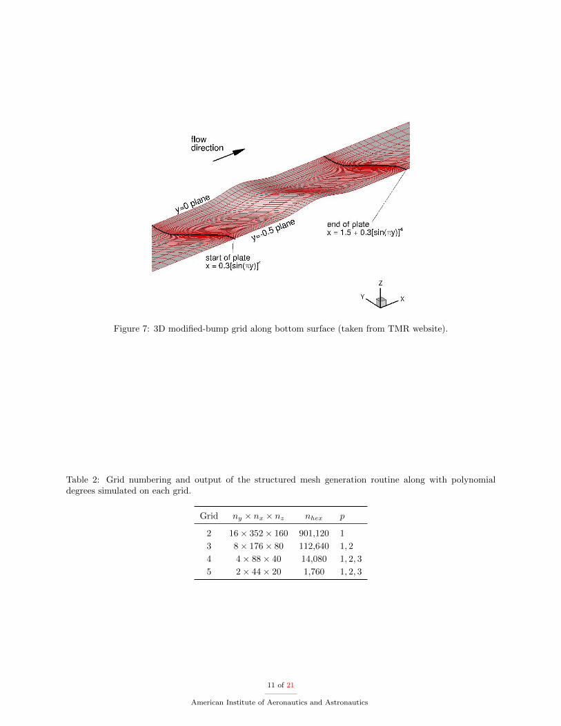
Figure 7: 3D modified-bump grid along bottom surface (taken from TMR website).

Table 2: Grid numbering and output of the structured mesh generation routine along with polynomialdegrees simulated on each grid.

Grid ny × nx × nz nhex p

2 16× 352× 160 901,120 1

3 8× 176× 80 112,640 1, 2

4 4× 88× 40 14,080 1, 2, 3

5 2× 44× 20 1,760 1, 2, 3

11 of 21


D. Mesh Curving

A parallel linear-elasticity solver is used to curve the modified bump mesh. The linear-elasticity solver isbased on a continuous Galerkin discretization and has line-solvers, multigrid, and high-order mixed elementcapabilities. The boundary conditions for the solver are specified by using surfaces from finer grids providedby the NASA turbulence resource website. For example, to curve grid 5 (2 × 44 × 20 hexahedra) with aquadratic mapping, the surfaces from grid 4 (4× 88× 40 hexahedra) are used and for a quartic mapping thesurfaces from grid 3 (8×176×80 hexahedra) are used. For the p = 1 modified bump simulations a quadraticmapping (q = 2) is used and for the p = 2, 3 simulations a quartic mapping (q = 4) mapping is used (notethis is higher than p+ 1 for the p = 2 simulation).

E. Results

Nine simulations were carried out for the modified-bump test case, varying polynomial degree and grid size(see Table 2). For all of these simulations, partitioning of the grid is performed based on lines. Since DGis a cell-based discretization, the lines are based on cells. The lines allow for a line-implicit Jacobi iterativemethod to be used as a preconditioner to the FGMRES linear solver. The preconditioner is applied amaximum of 200 iterations or until the residual drops 2 orders of magnitude. If the preconditioner beginsto diverge (relative residual rises to 1.5) the iterations are stopped prematurely and FGMRES moves on tothe next Krylov vector. Each linear system is solved 5 orders of magnitude and if the linear system fails toconverge then the CFL is lowered. Also, if a change in pressure or density is too large (greater than 20%)the CFL is lowered [19].

Figure 8 shows the iterative convergence of the simulation using grid 4 and polynomial degrees p = 1, 2, 3.In this series of simulations, the p = 1 simulation is initialized with free-stream flow, while the p = 2simulation is initialized using the p = 1 solution and then once again the p = 3 simulation is initialized usingthe p = 2 solution. For the first simulation (p = 1) the CFL number ramps up quickly until the turbulencemodel causes large changes in the solution at about iteration 15, the CFL adjusts and then begins to climbagain. Newton convergence begins at about iteration 42 and a total of 48 iterations are needed to reachmachine precision. Also, shown in this Figure is the iterative convergence of the drag which, as expected,closely follows the iterative convergence of the non-linear residual. The p = 2 simulation struggles to convergewith non-monotone CFL ramping and does not achieve Newton-like quadratic convergence, although it doesachieve a final residual norm of 10−10. Consequently, two changes were made to the inputs of the solver toimprove the convergence of the p = 3 simulation. The first is using a lower convergence tolerance on thelinear system, to only requiring 3 orders of relative residual reduction. This will allow the CFL number togrow larger than if 5 orders or convergence were required. The second change is an increase in the numberof quadrature points in the cell and face. It is believed (but not fully analyzed) that there are enoughnon-linearities in the mapping used for curving the mesh to cause issues in the non-linear convergence of thesolver.

All three of these simulations (grid 4, p = 1, 2, 3) are performed on 256 processors. For p = 1, there are1.1 × 105 DOF’s solved in 981 seconds, for p = 2, there are 3.8 × 105 DOF’s solved in 43,200 seconds, andfor p = 3, there are 9.0 × 105 DOF’s solved in 55,092 seconds. Typically, the p = 3 simulations are moretime consuming compared to the p = 2 simulations, however with the changes to the solver inputs, Newtonconvergence is obtained and this speeds up the overall time to solution. Similar non-linear convergence issuesoccurred on finer grids and the solver inputs had to be modified accordingly. For grid 2 it was observed thatthe non-linear convergence path could lead to a negative pressure if the CFL was too large in the beginningof the simulation. This might attributed to using a line-solver preconditioner perpendicular to the flowdirection and the lack of multigrid. As the grids get finer it takes more iterations for information to traveldownstream. Therefore, the CFL must not grow too quickly until the wake is developed enough.

For verification purposes a mesh resolution study is performed on drag and lift coefficient. Figure 9 showsthe drag coefficient broken into components, total drag coefficient, and lift coefficient for all nine simulations.Looking at the drag coefficient contribution from pressure in Figure 9a the p = 1 DG simulations convergessimilarly to CFL3D. All of the high-order DG simulations are mesh converged and are within one drag countof the mesh converged drag coefficient contribution from pressure. On the other hand, the drag coefficientcontribution from friction drag does not look mesh converged and appears to be converging to a slightlydifferent mesh converged solution although it is only around 0.25 of a drag count away from the finite-volume solvers. Figure 9c shows similar trends to the drag coefficient contribution from pressure. The p = 1

12 of 21


Figure 8: Iterative convergence of non-linear residual, CFL, and CD for grid 4, p = 1, 2, 3

DG simulations are similar to the CFL3D results and the higher-order DG simulations appear all meshresolved and within a drag count. Figure 9d shows the lift coefficient for all nine simulations. All of the DGsimulations are converging to similar lift coefficients as FUN3D and USM3D. The p = 2, 3 DG simulationsare converging to the mesh resolved lift coefficient using fewer degrees of freedom compared to the p = 1simulation and all of the finite-volume solvers.

The computed surface pressure coefficients (CP ) are shown in Figure 10 for six out of nine simulationsfor the modified-bump problem. The CP is plotted along a line in the axial direction (x-direction) at y = 0.Only grids 2-4 are shown because the grid 5 solutions are not resolved enough, due to only two elementsbeing used in the span direction. When comparing to the FUN3D results only the grid 3, p = 2 and thegrid 4, p = 3 simulations are mesh resolved. The remaining simulations are still not resolved enough. Thisis surprising given the accuracy shown for almost all cases in the mesh resolution study. This shows theimportance of showing solution profiles and not just integrated values.

VII. High Lift Prediction of the DLR-F11

The second AIAA CFD High Lift Prediction Workshop (HiLiftPW-2) was held in June 2013. The focusof this workshop was on the validation of numerical methods for a realistic high-lift configuration of a moderntransport aircraft. The DLR-F11 experiment was chosen for this purpose [28]. The DLR-F11 is a wing-bodyconfiguration with a full span leading-edge slat and single-slotted trailing-edge flap. A slat deflection of 26.5degrees and a flap deflection of 32 degrees are specified for the workshop test cases. In this section, theresults of the DLR-F11 simulation using the DG solver will be compared to results from a state-of-the-artfinite-volume solver: NSU3D [29]. It is important to note that the DG solver uses the negative variant ofthe SA turbulence model and NSU3D uses the original SA model.


The flow conditions are: angle of attack α = 7o and α = 16o , Mach = 0.175, Re = 1.51 × 107, γ = 1.4,Pr = 0.72, and Prt = 0.9. The problem is initialized using uniform flow at the free-stream conditions. Theturbulence equation is initialized everywhere as ρνt∞ = 3µ∞/µ

′. The far-field boundary conditions consistof non-reflecting Riemann invariants where the far-field values are taken as the free-stream conditions given

13 of 21


(a) Drag coefficient contribution from pressure. (b) Drag coefficient contribution from friction drag.

(c) Total drag coefficient. (d) Total lift coefficient.

Figure 9: Drag and lift coefficient versus mesh size for the modified-bump compared to FUN3D, USM3D,and CFL3D.

14 of 21


(a) (b)

(c) Close up view. (d) Close up view.

Figure 10: Computed surface pressure coefficients CP for the modified-bump on grids 2-4 compared toFUN3D results on the finest grid.

15 of 21


above.

B. Grid, Wall Distance, and Mesh Curving

The geometry for this simulation comes from Case 1 of the HiLiftPW-2 and consists of a simple clean wing-slat-flap system with no fairings, supports or brackets. The grid is generated using VGRID and is similarto the grids used for the workshop [29]. The grid consists of 2.8 × 106 prisms, 4.4 × 104 pyramids, and3.0× 106 tetrahedra. The grid is shown in Figure 14. Compared to the grids in [29] this grid is coarser thanthe coarsest grid but because of the cell-based DG discretization, the degrees of freedom, using a p = 1 DGdiscretization, are comparable to the medium grid using a finite-volume discretization. The wall distance iscalculated using a brute force search method on straight edged triangular faces. This is identical to the walldistance calculation discussed previously in section VI.C.

The DLR-F11 mesh is curved by first subdividing each face on the surface into self similar elements.This creates a new set of points which are snapped back onto the CAD geometry using Open Cascade [30].However, the new points can cause negative volumes in the DG simulation. To address this, the newly createdpoints are treated as boundary conditions to the linear elasticity solver previously discussed in VI.D. Thelinear elasticity solver curves the volume cells such that all of the negative volumes are properly eliminated.

C. Results

Two simulations were carried out for the DLR-F11 high-lift configuration varying only angle of attack (α = 7

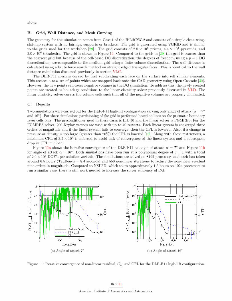
and 16). For these simulations partitioning of the grid is performed based on lines on the prismatic boundarylayer cells only. The preconditioner used in these cases is ILU(0) and the linear solver is FGMRES. For theFGMRES solver, 200 Krylov vectors are used with up to 40 restarts. Each linear system is converged threeorders of magnitude and if the linear system fails to converge, then the CFL is lowered. Also, if a change inpressure or density is too large (greater than 20%) the CFL is lowered [19]. Along with these restrictions, amaximum CFL of 3.5 × 104 is enforced to avoid lack of convergence of the linear system and a subsequentdrop in CFL number.

Figure 11a shows the iterative convergence of the DLR-F11 at angle of attack α = 7 and Figure 11bfor angle of attack α = 16. Both simulations have been run at a polynomial degree of p = 1 with a totalof 2.9× 107 DOF’s per solution variable. The simulations are solved on 8192 processors and each has takenaround 6.5 hours (TauBench = 8.4 seconds) and 550 non-linear iterations to reduce the non-linear residualnine orders in magnitude. Compared to NSU3D, which takes approximately 1.5 hours on 1024 processors torun a similar case, there is still work needed to increase the solver efficiency of DG.

(a) Angle of attack 7 (b) Angle of attack 16

Figure 11: Iterative convergence of non-linear residual, CL, and CFL for the DLR-F11 high-lift configuration.

16 of 21


A mesh resolution study can not be performed with only one data point for each angle of attack. There-fore, a strong argument can not be made when comparing the forces with the experiments and NSU3Ddata. Figure 12a shows the drag coefficient and the DG simulations show very similar results to the mediumNSU3D grids. Figure 12b shows the lift coefficient and the DG simulation matches closer to the experimentat the lower angle of attack but slightly farther from the experimental value compared to NSU3D for thehigher angle of attack. Figure 12c shows the Moment coefficient and both the DG simulation and NSU3Dare far away from the experimental values. The DG simulation is similar to NSU3D at the higher angle ofattack and somewhere in between the experiment and NSU3D at the lower angle of attack. Again, it is hardto draw many conclusions since there is only one data point for the DG simulations.

(a) Drag coefficient. (b) Lift coefficient. (c) Moment coefficient.

Figure 12: Coefficients of drag, lift, and moment for the DLR-F11 at angles of attack α = 7 and 16

compared to experiments and NSU3D.

The computed surface pressure coefficients (CP ) are shown in Figure 13 for the DLR-F11 at stations 1,6and 10 for both angles of attack. Overall, the DG simulations compare well with NSU3D and the experiments.The only major discrepancies occur at station 10, α = 7 on the flap where a region of separation is observedin the DG simulation but not in the experiment or NSU3D. Further investigation into these discrepanciesshowed that FUN3D also observed separation at station 10 and α = 16 [31]. But they did not observe thisuntil they performed several mesh adaption steps (using adjoint) resulting in 6 × 107 degrees of freedom.Since FUN3D only performed adaption at the higher angle of attack it is not clear if the separation shouldbe observed at the lower angle of attack near station 10 as seen in the DG simulations. Contours of CP areshown on the surface of the DLR-F11 in Figure 14 for α = 16. Clearly, in the outboard span area of thewing there is a region of lower CP on the flap in the DG simulation.

VIII. Conclusions

In this work, mesh resolved simulations are performed of the 3D hemisphere-cylinder and the 3D modified-bump. The NASA TMR website provides grids and reference solutions for the FUN3D, CFL3D, and USM3Dsolvers. These solutions are compared to DG simulations using a p-refinement study and a h-refinementstudy. Overall, the DG solver compares well with the finite-volume solvers. For the hemisphere, the finite-volume solvers are not fully mesh resolved. However on the finer grids and with higher polynomial degreesthe DG simulations are mesh resolved. The bump is closer to being mesh resolved for the finite-volumesolvers and again the DG solver compares well. The DG solver in both of these cases converges to themesh resolved answers with fewer degrees of freedom using a higher order of accuracy, which is typical ofhigh-order methods.

In terms of non-linear convergence the DG solver performs well for the hemisphere case. For all of thegrids and polynomial degree p = 1, it takes around 40 non-linear iterations to solve to machine precision.This is due to the Newton-Krylov solver with line preconditioning and the CFL controller [19]. When thelower order solutions are used to initialize the higher order solutions even fewer iterations are required.

17 of 21


(a) Station 1, α = 7 (b) Station 6, α = 7 (c) Station 10, α = 7

(d) Station 1, α = 16 (e) Station 6, α = 16 (f) Station 10, α = 16

Figure 13: Computed surface pressure coefficients CP for the DLR-F11 compared to NSU3D results on thefinest grid and experimental data.

18 of 21


The bump performs almost as well the hemisphere but convergence is more challenging on the finer grids.Relaxing the tolerances on the linear solve helps with achieving Newton quadratic convergence in this case.

The simulation of the DLR-F11 compares well to NSU3D results for both angles of attack α = 7 andα = 16. Only one p = 1 simulation was performed at each angle of attack, so not many conclusions can bedrawn from these comparisons. The drag, lift, and moment coefficients compare well with NSU3D. Also, CPline plots at stations 1 and 6 at both angles of attack compare well with NSU3D. Separation was observedat station 10, α = 7, in the DG solution that is not observed in NSU3D or the experiments. However,separation at station 10, α = 16, is observed again in the DG solution but also occurs in a mesh adaptedsolution using FUN3D. This needs to be further investigated along with running finer grids and higher ordersof accuracy.

IX. Acknowledgments

Computer time was provided by the NCAR-Wyoming Supercomputing Center (NWSC) and Universityof Wyoming Advanced Research Computing Center (ARCC).

References

1Rumsey, C., “Turbulence Modeling Resource,” turbmodels.larc.nasa.gov, August 2014.2Fidkowski, K. J. and Darmofal, D. L., “An adaptive simplex cut-cell method for discontinuous Galerkin discretizations

of the Navier-Stokes equations,” AIAA Paper , Vol. 3941, 2007, pp. 2007.3Wang, L. and Mavriplis, D. J., “Adjoint-based h–p adaptive discontinuous Galerkin methods for the 2D compressible

Euler equations,” Journal of Computational Physics, Vol. 228, No. 20, 2009, pp. 7643–7661.4Hartmann, R. and Houston, P., “Adaptive discontinuous Galerkin finite element methods for the compressible Euler

equations,” Journal of Computational Physics, Vol. 183, No. 2, 2002, pp. 508–532.5Ahrabi, B. R., Anderson, W. K., and Newman, J. C., High-Order Finite-Element Method and Dynamic Adaptation

for Two-Dimensional Laminar and Turbulent Navier-Stokes, AIAA Paper 2014-2983, 32nd AIAA Applied AerodynamicsConference, Atlanta GA, June 2014.

6Ahrabi, B. R., Anderson, W. K., and Newman, J. C., An Adjoint-Based hp-Adaptive Petrov-Galerkin Method for Tur-bulent Flows, AIAA Paper 2015-2603, 22nd AIAA Computational Fluid Dynamics Conference, Dallas, TX, June 2015.

7Brazell, M. J. and Mavriplis, D. J., 3D Mixed Element Discontinuous Galerkin with Shock Capturing, AIAA Paper2013-2855, 21st AIAA CFD Conference, San Diego, CA, June 2013.

8Diskin, B., Thomas, J., Rumsey, C. L., and Schwoeppe, A., Grid Convergence for Turbulent Flows (Invited), AIAAPaper 2015-1746, 53rd AIAA Aerospace Sciences Meeting, Kissimmee, FL, January 2015.

9Brazell, M. J. and Mavriplis, D. J., High-Order Discontinuous Galerkin Mesh Resolved Turbulent Flow Simulations of aNACA 0012 Airfoil (Invited), AIAA Paper 2015-1529, 53rd AIAA Aerospace Sciences Meeting, Kissimmee, FL, January 2015.

10Ceze, M. and Fidkowski, K., High-Order Output-Based Adaptive Simulations of Turbulent Flow in Two Dimensions(Invited), AIAA Paper 2015-1532, 53rd AIAA Aerospace Sciences Meeting, Kissimmee, FL, January 2015.

11Hu, Y., Wagner, C., Allmaras, S., Galbraith, M., and Darmofal, D. L., Application of a Higher-order Adaptive Method toRANS Test Cases (Invited), AIAA Paper 2015-1530, 53rd AIAA Aerospace Sciences Meeting, Kissimmee, FL, January 2015.

12Anderson, W. K., Ahrabi, B. R., and Newman, J., Finite-Element Solutions for Turbulent Flow over the NACA 0012Airfoil (Invited), AIAA Paper 2015-1531, 53rd AIAA Aerospace Sciences Meeting, Kissimmee, FL, January 2015.

13Rumsey, C. L., Biedron, R. T., and Thomas, J. L., CFL3D, Its History and Some Recent Applications, Vol. 112861,National Aeronautics and Space Administration, Langley Research Center, 1997.

14Anderson, W. K. and Bonhaus, D. L., “An implicit upwind algorithm for computing turbulent flows on unstructuredgrids,” Computers & Fluids, Vol. 23, No. 1, 1994, pp. 1–21.

15Frink, N. T., “Tetrahedral Unstructured Navier-Stokes Method for Turbulent Flows,” AIAA Journal , Vol. 36, No. 11,2015/12/08 1998, pp. 1975–1982.

16Rumsey, C., “2nd AIAA CFD High Lift Prediction Workshop,” http://hiliftpw.larc.nasa.gov/index-workshop2.html, May2015.

17Spalart, P. and Allmaras, S., A one-equation turbulence model for aerodynamic flows, Vol. 1, Le Recherche Aerospatiale,1994, pp. 5–21.

18Allmaras, S., Johnson, F., and Spalart, P., “Modifications and Clarifications for the Implementation of the Spalart-Allmaras Turbulence Model,” 7th International Conference on Computational Fluid Dynamics, 2012.

19Ceze, M. A. and Fidkowski, K. J., “Constrained pseudo-transient continuation,” International Journal for NumericalMethods in Engineering, Vol. 102, 2015, pp. 1683–1703.

20Lax, P. D., “Weak solutions of nonlinear hyperbolic equations and their numerical computation,” Communications onPure and Applied Mathematics, Vol. 7, No. 1, 1954, pp. 159–193.

21Roe, P., “Approximate Riemann solvers, parameter vectors, and difference schemes,” J. Comput. Phys. (USA), Vol. 43,No. 2, 1981/10/, pp. 357 – 72.

22Sun, M. and Takayama, K., “An artificially upstream flux vector splitting scheme for the Euler equations,” J. Comput.Phys. (USA), Vol. 189, No. 1, 2003/07/20, pp. 305 – 29.

19 of 21


23Hartmann, R. and Houston, P., “An optimal order interior penalty discontinuous Galerkin discretization of the compress-ible Navier-Stokes equations,” J. Comput. Phys. (USA), Vol. 227, No. 22, 2008/11/20, pp. 9670 – 85.

24Shahbazi, K., Mavriplis, D., and Burgess, N., “Multigrid algorithms for high-order discontinuous Galerkin discretizationsof the compressible Navier-Stokes equations,” J. Comput. Phys. (USA), Vol. 228, No. 21, 2009/11/20, pp. 7917 – 40.

25Burgess, N. K. and Mavriplis, D. J., “An hp-adaptive Discontinuous Galerkin solver for aerodynamic flows on mixed-element meshes,” AIAA Paper 2011-490, 49th AIAA Aerospace Sciences Meeting Including the New Horizons Forum andAerospace Exposition, January 2011.

26Saad, Y., “A flexible inner-outer preconditioned GMRES algorithm,” SIAM J. Sci. Comput., Vol. 14, No. 2, March 1993,pp. 461–469.

27Hsieh, T., “An Investigation of Separated Flow about a Hemisphere-Cylinder at 0- to 19-Deg Incidence in the MachNumber Range from 0.6 to 1.5,” Tech. rep., AEDC-TR-76-112, 1974.

28Rudnik, R., Huber, K., and Melber-Wilkending, S., EUROLIFT Test Case Description for the 2nd High Lift PredictionWorkshop, AIAA Paper 2012-2924, 30th AIAA Applied Aerodynamics Conference, June 2012.

29Mavriplis, D., Long, M., Lake, T., and Langlois, M., “NSU3D Results for the Second AIAA High-Lift Prediction Work-shop,” Journal of Aircraft , Vol. 52, No. 4, 2015/11/22 2015, pp. 1063–1081.

30“OpenCascade - an open source library for BRep solid modeling,” http://www.opencascade.com, 2000.31Lee-Rausch, E. M., Rumsey, C. L., and Park, M. A., “Grid-Adapted FUN3D Computations for the Second High-Lift

Prediction Workshop,” Journal of Aircraft , Vol. 52, No. 4, 2015/11/29 2015, pp. 1098–1111.

20 of 21


Figure 14: Contours of computed surface pressure coefficients CP for the DLR-F11 at α = 16 and mesh.

21 of 21


discontinuous galerkin turbulent flow simulations of · pdf fileow over a hemisphere-cylinder...

Documents