discontinuous spectral element method for solving...

ARTICLE IN PRESS

Journal of Quantitative Spectroscopy &

0022-4073/$ - se

doi:10.1016/j.jq

�CorrespondE-mail addr

Radiative Transfer 107 (2007) 1–16

www.elsevier.com/locate/jqsrt

Discontinuous spectral element method for solving radiativeheat transfer in multidimensional semitransparent media

J.M. Zhao, L.H. Liu�

School of Energy Science and Engineering, Harbin Institute of Technology, 92 West Dazhi Street, Harbin 150001, People’s Republic of China

Received 16 December 2006; received in revised form 29 January 2007; accepted 4 February 2007

Abstract

A discontinuous spectral element method (DSEM) is presented to solve radiative heat transfer in multidimensional

semitransparent media. This method is based on the general discontinuous Galerkin formulation. Chebyshev polynomial is

used to build basis function on each element and both structured and unstructured elements are considered. The DSEM

has properties such as hp-convergence, local conservation and its solutions are allowed to be discontinuous across

interelement boundaries. The influences of different schemes for treatment of the interelement numerical flux on the

performance of the DSEM are compared. The p-convergence characteristics of the DSEM are studied. Four various test

problems are taken as examples to verify the performance of the DSEM, especially the performance to solve the problems

with discontinuity in the angular distribution of radiative intensity. The predicted results by the DSEM agree well with the

benchmark solutions. Numerical results show that the p-convergence rate of the DSEM follows exponential law, and the

DSEM is stable, accurate and effective to solve multidimensional radiative transfer in semitransparent media.

r 2007 Elsevier Ltd. All rights reserved.

Keywords: Discontinuous Galerkin method; Spectral element method; Radiative heat transfer; Ray effect

1. Introduction

Numerical methods for solving radiative transfer can be classified into two types, one is the method basedon the discretization of radiative transfer equation, and the other is the method based on ray-tracingtechnique. In recent years, the method based on the discretization of radiative transfer equation, such asdiscrete ordinate method (DOM) [1], finite-volume method (FVM) [2–4], and finite-element method (FEM)[5,6], have received considerable attention for their advantages such as being flexible to deal with complexmedia and boundary property, easy and efficient to treat multidimensional problems as compared to the ray-tracing-based methods, such as Monte Carlo method [7] and zonal method [8].

Recently, the discontinuous Galerkin (DG) method was introduced to the solution of radiative transferproblems. Cui and Li [9,10] presented a DG FEM for solving the radiative transfer in emitting, absorbing, andscattering media, in which the linear approximation was used on each element. Liu et al. [11] applied the DG

e front matter r 2007 Elsevier Ltd. All rights reserved.

srt.2007.02.001

ing author. Tel.: +86451 86402237; fax: +86 451 86221048.

ess: [email protected] (L.H. Liu).

www.elsevier.com/locate/jqsrt

dx.doi.org/10.1016/j.jqsrt.2007.02.001

mailto:[email protected]

ARTICLE IN PRESS

Nomenclature

H matrix defined in Eqs. (14b) and (15b)I radiative intensity, W/(m2sr)Ib black body radiative intensity, W/(m2sr)K the kth elementKtr triangular elementKst standard elementM number of discrete ordinate directionM matrix defined in Eqs. (14a) and (15a)n unit outward normal vectornqK unit outward normal vector of the boundary of element K

Nel total number of elementsNsol total number of solution nodesp order of polynomial expansionq radiative heat flux, W/m2

r spatial coordinates vectorS source term function defined by Eq. (2)T temperature, Kw weight of discrete ordinates approximationW weight functionx, y, z cartesian coordinatesb extinction coefficient b ¼ ðkþ sSÞ, m

�1

ew wall emissivityf nodal basis functionF scattering phase functionm, Z, x direction cosine of radiation directionk absorption coefficient, m�1

sS scattering coefficient, m�1

s Stefan-Boltzmann constant, W/(m2K4)tL optical thickness, tL ¼ bL

o single scattering albedoX, X0 unit vector of radiation directionO solid anglez, g, B cartesian coordinates defined in standard element

Subscripts

i, j spatial node indexw value at wall

Superscripts

m, m0 the mth discrete ordinate direction

J.M. Zhao, L.H. Liu / Journal of Quantitative Spectroscopy & Radiative Transfer 107 (2007) 1–162

FEM to solve radiative transfer in graded index media. All of these works initially demonstrated that the DGapproach is a very promising method for the solution of radiative transfer problems in both regular andirregular geometries using either structured or unstructured meshes. The DG method has many advantagescomparing to the conventional Galerkin method and has been successfully applied to the solution of manyphysics and engineering problems [12–15]. In DG method, the inter-element continuity is released and the

ARTICLE IN PRESSJ.M. Zhao, L.H. Liu / Journal of Quantitative Spectroscopy & Radiative Transfer 107 (2007) 1–16 3

approximation space composes of discontinuous functions. The DG method is considered to combine both theadvantages of FVM and FEM. The main virtues of the DG method can be summarized as: (1) it is element-wise conservative and stable, (2) high-order accurate and polynomials of arbitrary degree can be employed ateach element, which make the DG method ideal to be used with hp-adaptive strategies, (3) the method can bedefined on very general meshes, including non-conforming meshes and (4) it is easy to be implemented andsolved element by element. Introduction and comprehensive review of the DG method are referred toCockburn et al. [16,17].

Spectral-element method (SEM) was originally proposed by Patera [18] for the solution of fluid flowproblem. In the SEM, the physical domain is broken up into several elements and within each element aspectral representation based on orthogonal polynomials (such as Chebyshev polynomial and Legendrepolynomial) is used. SEM combines the competitive advantages of high-order spectral method, i.e. the p-convergence property, and FEM, i.e. the flexibility to deal with complex domain and offering h-convergenceproperty. SEM has been successfully applied in computational fluid dynamics and heat transfer [18–21].Recently, by considering that the equation of radiative transfer (RTE) is in a form of convection-dominatedequation [22] and the convection term may cause non-physical oscillation of the solutions of standardGalerkin scheme-based methods, Zhao and Liu [23,24] developed a least-square SEM (LSSEM) for solvingmultidimensional radiative transfer problems in uniform and graded index media, in which the least-squarescheme instead of the standard Galerkin scheme of SEM (GSEM) is used to enhance the stability of themethod to solve the RTE. These works demonstrated that higher-order spectral approximation on eachelement is effective to solve multidimensional radiative transfer problems. However, both the GSEM and theLSSEM are based on global continuous formulation, in which the functions of approximation space are notallowed to be discontinuous across elements, thus lack the salient properties of the method based on the DGformulation described above.

To combine both the advantages of the SEM and the DG method, in this paper, based on the general DGformulation, we present a discontinuous SEM (DSEM) to solve radiative heat transfer in multidimensionalsemitransparent media, in which Chebyshev polynomial is used to build basis function on each element. Theinfluences of different schemes for the treatment of interelement numerical flux are compared and the p-convergence characteristics of the DSEM are studied. The performance of the DSEM is verified by various testexamples on meshes with both structured and unstructured elements.

2. Mathematical formulation

2.1. Discrete-ordinates equation of radiative transfer

The discrete-ordinates equation of radiative transfer in the enclosure filled with absorbing, emitting, andscattering gray media can be written in Cartesian coordinates as

rd XmImðrÞ½ � þ bImðrÞ ¼ SmðrÞ, (1)

where the source term Sm(r) is defined as

SmðrÞ ¼ kIbðrÞ þsS4p

XMm0¼1

Im0 ðrÞUðXm;Xm0Þwm0 . (2)

For the opaque and diffuse boundary, the boundary conditions are given as

Imw ¼ �wIbw þ

1� �wp

XnwdXm040

Im0

w nwdXm0�� wm0 ;Xmdnwo0, (3)

where Xm is the discrete direction vector, b ¼ ðkþ sSÞ is the extinction coefficient, k and sS are the absorptionand scattering coefficients, respectively, F is the scattering phase function, ew is the wall emissivity and wm0 isthe weight of direction Xm0 for angular quadrature.

The partial differential Eq. (1) with boundary condition given by Eq. (3) is solved for each discrete direction.The discrete ordinates equation Eq. (1) is in a form as a convection-dominated equation [22]. The convection

ARTICLE IN PRESSJ.M. Zhao, L.H. Liu / Journal of Quantitative Spectroscopy & Radiative Transfer 107 (2007) 1–164

term may cause non-physical oscillatory of solutions. This type of instability can occur in many numericalmethods including finite difference method and FEM if no special stability treatment is taken. In Section 2.2, aDSEM was developed to solve the discrete-ordinates equation of radiative heat transfer.

2.2. General DG formulation

Unlike the continuous Galerkin solution scheme, which uses global basis function and weight function, theDG scheme uses basis and weight function locally defined on each element. In DG solution scheme, theinformation transfer across element boundaries is imposed by modeling the numerical flux. Details ondescription and discussion of the features of the DG method are referred to Ref. [16]. For each element K, Eq.(1) is weighted by W and integrated over K using Gauss divergence theorem

�oI ;XdrW4K þ ðcXIdnqK ;W ÞqK þobI ;W4K ¼oS;W4K . (4)

Without ambiguity the superscript m is omitted, where nqK denotes the unit outward normal vector of theboundary of element K and the operators od; d4 and ðd; dÞ are defined as

of ; g4K ¼

ZK

fgdV ; ðf ; gÞqK ¼

ZqK

fgdA, (5)

Here, cXI is the numerical flux across element boundaries to be modeled. In this paper, two numerical schemesare considered to model cXI . The first scheme considered is the classical up-winding scheme, in which thenumerical flux is modeled as

cXI ¼ X If g þX signðXdnqK Þ1IU, (6)

where the operator fdg and 1dU� denote the mean value and the jump value of arguments across interelementboundary

If g ¼1

2Iþ þ I��

; 1IU� ¼1

2Iþ � I��

. (7)

Here the superscript operator ‘‘+’’ and ‘‘�’’ denote the values at the boundary inside element K and outsideelement K, respectively, which are defined as

Iþ ¼ limd!0

IðrqK � dnqK Þ; I� ¼ limd!0

Iðr@K þ dn@K Þ. (8)

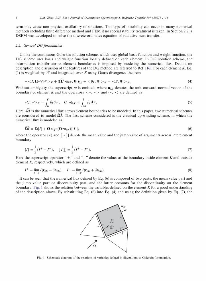
It can be seen that the numerical flux defined by Eq. (6) is composed of two parts, the mean value part andthe jump value part or discontinuity part, and the latter accounts for the discontinuity on the elementboundary. Fig. 1 shows the relation between the variables defined on the element K for a good understandingof the description above. By substituting Eq. (6) into Eq. (4) and using the definition given by Eq. (7), the

K

n∂K

+−

−

+

+

+

I +

I −

Ω I

Ω

Fig. 1. Schematic diagram of the relations of variables defined in discontinuous Galerkin formulation.


general DG formulation of RTE for up-winding scheme is obtained as

�oI ;XdrW4K þ1

2XdnqK þ XdnqKj jð ÞIþ;W� �

qKþobI ;W4K

¼oS;W4K �1

2XdnqK � XdnqKj jð ÞI�;Wð ÞqK . ð9Þ

The second scheme considered is the local Lax-Friedrichs scheme. The numerical flux is modeled as

cXI ¼ X If g þ Xj j1IUnqK . (10)

The general DG formulation of RTE for local Lax-Friedrichs scheme is obtained as

�oI ;XdrW4K þ1

2XdnqK þ Xj jð ÞIþ;W� �

qKþobI ;W4K

¼oS;W4K �1

2XdnqK � Xj jð ÞI�;Wð ÞqK . ð11Þ

It should be noted that the modulus |X| is |m|,ffiffiffiffiffiffiffiffiffiffiffiffiffiffiffim2 þ Z2

pand 1 for one-, two- and three-dimensional problem,

respectively. It can be seen that Eqs. (9) and (11) are identical in one-dimensional case.

2.3. Spectral element discretization

Here, the nodal basis functions on each element are constructed by Chebyshev polynomial expansion. Theone-dimensional nodal basis functions are Lagrange interpolation polynomials through the Cheby-shev–Gauss–Lobatto points. Multidimensional nodal basis functions on structured element (quadrilateral,cube) are constructed by tensor product from one-dimensional nodal basis functions. The construction ofnodal basis functions on quadrilateral element was described detailedly in Ref. [23]. For the construction ofnodal basis functions on triangular element, if we consider the triangular as a degenerated quadrilateral,namely, with four nodes as shown in Fig. 2, then the same tensor product procedure can be used to build thenodal basis function on the triangular element Ktr. But special treatment on the nodal basis of node 1 of thetriangular element Ktr is still needed. The nodal basis function of node 1 of Ktr is selected as the sumof all nodal basis functions mapped from edge 4 (defined by nodes 1 and 4) of the standard quadrilateralelement Kst.

The unknown radiative intensity is approximated on element K by nodal basis function with KroneckerDelta property as

IðrÞ ’XNsk

i¼1

I ifiðrÞ, (12)

where fi is the nodal basis function defined on K, Ii denotes radiative intensity at solution nodes i and Nsk isthe number of solution nodes on K. By substituting the approximation of radiative intensity (Eq. (12)) into theDG formulation of RTE (Eq. (9) or Eq. (11)) and taking the weight function W as nodal basis function fj(r),the DSEM discretization of the RTE can be written in matrix form on element K as

MmIm ¼ Hm, (13)

γ

x

Kst

Ktr

(1,-1)

(1,1)

(-1,-1)

(-1,1)

2

y ζ1 2

4 3

3

1(4)

Fig. 2. Schematic diagram of the coordinates transform from stand element to triangular element.


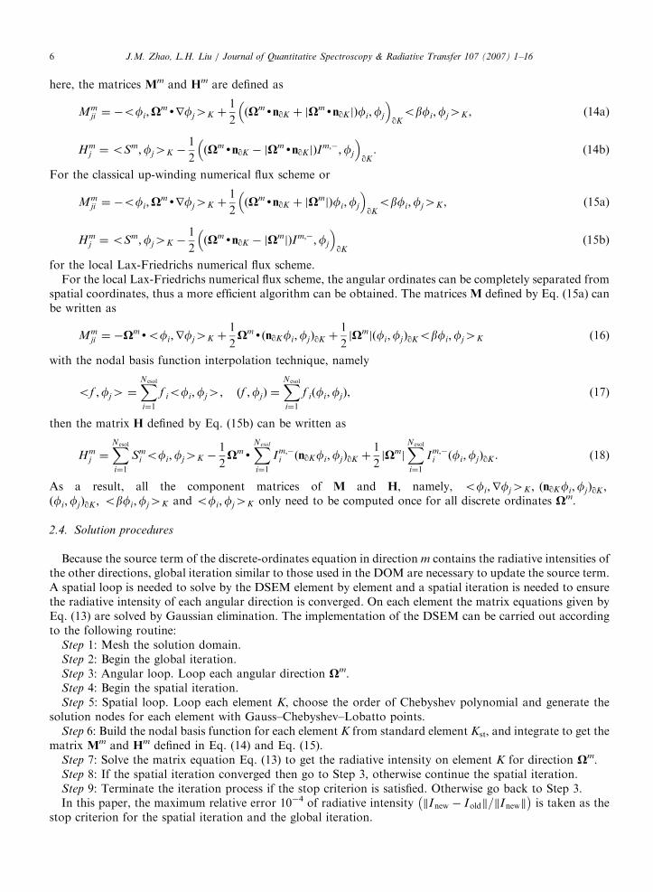
here, the matrices Mm and Hm are defined as

Mmji ¼ �ofi;X

mdrfj4K þ1

2XmdnqK þ XmdnqKj jð Þfi;fj

� �qKobfi;fj4K , (14a)

Hmj ¼oSm;fj4K �

1

2XmdnqK � XmdnqKj jð ÞIm;�;fj

� �qK. (14b)

For the classical up-winding numerical flux scheme or

Mmji ¼ �ofi;X

mdrfj4K þ1

2XmdnqK þ Xmj jð Þfi;fj

� �qKobfi;fj4K , (15a)

Hmj ¼oSm;fj4K �

1

2XmdnqK � Xmj jð ÞIm;�;fj

� �qK

(15b)

for the local Lax-Friedrichs numerical flux scheme.For the local Lax-Friedrichs numerical flux scheme, the angular ordinates can be completely separated from

spatial coordinates, thus a more efficient algorithm can be obtained. The matrices M defined by Eq. (15a) canbe written as

Mmji ¼ �Xmdofi;rfj4K þ

1

2XmdðnqKfi;fjÞqK þ

1

2Xmj jðfi;fjÞqKobfi;fj4K (16)

with the nodal basis function interpolation technique, namely

of ;fj4 ¼XNesol

i¼1

f iofi;fj4; ðf ;fjÞ ¼XNesol

i¼1

f iðfi;fjÞ, (17)

then the matrix H defined by Eq. (15b) can be written as

Hmj ¼

XNesol

i¼1

Smi ofi;fj4K �

1

2Xmd

XNesol

i¼1

Im;�i ðnqKfi;fjÞqK þ

1

2Xmj j

XNesol

i¼1

Im;�i ðfi;fjÞqK . (18)

As a result, all the component matrices of M and H, namely, ofi;rfj4K ; ðnqKfi;fjÞqK ;ðfi;fjÞqK ; obfi;fj4K and ofi;fj4K only need to be computed once for all discrete ordinates Xm.

2.4. Solution procedures

Because the source term of the discrete-ordinates equation in direction m contains the radiative intensities ofthe other directions, global iteration similar to those used in the DOM are necessary to update the source term.A spatial loop is needed to solve by the DSEM element by element and a spatial iteration is needed to ensurethe radiative intensity of each angular direction is converged. On each element the matrix equations given byEq. (13) are solved by Gaussian elimination. The implementation of the DSEM can be carried out accordingto the following routine:

Step 1: Mesh the solution domain.Step 2: Begin the global iteration.Step 3: Angular loop. Loop each angular direction Xm.Step 4: Begin the spatial iteration.Step 5: Spatial loop. Loop each element K, choose the order of Chebyshev polynomial and generate the

solution nodes for each element with Gauss–Chebyshev–Lobatto points.Step 6: Build the nodal basis function for each element K from standard element Kst, and integrate to get the

matrix Mm and Hm defined in Eq. (14) and Eq. (15).Step 7: Solve the matrix equation Eq. (13) to get the radiative intensity on element K for direction Xm.Step 8: If the spatial iteration converged then go to Step 3, otherwise continue the spatial iteration.Step 9: Terminate the iteration process if the stop criterion is satisfied. Otherwise go back to Step 3.In this paper, the maximum relative error 10�4 of radiative intensity Inew � Ioldk k= Inewk k

� �is taken as the

stop criterion for the spatial iteration and the global iteration.


3. Results and discussion

To verify the performance of the DSEM presented in this paper, four various test cases are selected. For thesake of quantitative comparison to the benchmark results, the integration averaged relative error of theDSEM solution is defined as

Relative error % ¼

RDSEM solution� Benchmark resultj jdxR

Benchmark resultj jdx� 100. (19)

3.1. Case 1: Gaussian-shaped radiative source term between infinite parallel black plates

We consider the radiative transfer between one-dimensional black parallel plates. The radiative source termwithin the media is a Gaussian-shaped function. This problem is modeled by the RTE as

mdI

dxþ bI ¼ e�ðx�cÞ2=a2 ; x; c 2 ½0; 1� (20)

with the following boundary conditions:

Ið0;mÞ ¼ e�c2=a2 ; m40, (21a)

Ið0;mÞ ¼ e�ð1�cÞ2=a2 ; mo0. (21b)

The analytical solution of this problem in the case of m40 can be written as

Iðx;mÞ ¼ Ið0;mÞ exp �bx

m

� �

affiffiffipp

2mexp �

bm

x�a2b4mþ c

� �� erf

ab2mþ

c� x

a

� � erf

ab2mþ

c

a

� �.

(22)

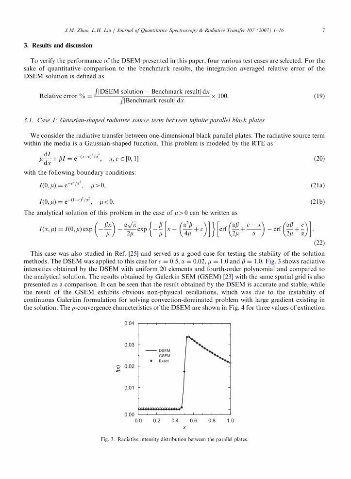
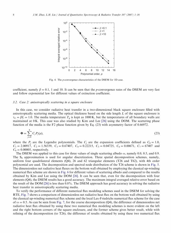
This case was also studied in Ref. [25] and served as a good case for testing the stability of the solutionmethods. The DSEM was applied to this case for c ¼ 0.5, a ¼ 0.02, m ¼ 1.0 and b ¼ 1.0. Fig. 3 shows radiativeintensities obtained by the DSEM with uniform 20 elements and fourth-order polynomial and compared tothe analytical solution. The results obtained by Galerkin SEM (GSEM) [23] with the same spatial grid is alsopresented as a comparison. It can be seen that the result obtained by the DSEM is accurate and stable, whilethe result of the GSEM exhibits obvious non-physical oscillations, which was due to the instability ofcontinuous Galerkin formulation for solving convection-dominated problem with large gradient existing inthe solution. The p-convergence characteristics of the DSEM are shown in Fig. 4 for three values of extinction

0.0 0.2 0.4 0.6 0.8 1.00.00

0.01

0.02

0.03

0.04

DSEM

GSEM

Exact

x

I(x)

Fig. 3. Radiative intensity distribution between the parallel plates.

ARTICLE IN PRESS

0 2 4 6 8 10 12 14 1610-10

10-8

10-6

10-4

10-2

100

� =0.1

� =1

� =10

Polynomial order, p

Inte

gra

l avera

ged r

ela

tive e

rror

Fig. 4. The p-convergence characteristics of the DSEM for 1D case.


coefficient, namely b ¼ 0.1, 1 and 10. It can be seen that the p-convergence rates of the DSEM are very fastand follow exponential law for different values of extinction coefficient.

3.2. Case 2: anisotropically scattering in a square enclosure

In this case, we consider radiative heat transfer in a two-dimensional black square enclosure filled withanisotropically scattering media. The optical thickness based on the side length L of the square enclosure istL ¼ bL ¼ 1:0. The media temperature Tg is kept as 1000K, but the temperatures of all boundary walls aremaintained at 0K. This case was also studied by Kim and Lee [26] using the DOM. The scattering phasefunction of the media is the F2 phase function given by Eq. (23) with asymmetry factor of 0.66972.

U ¼X8j¼0

CjPjðmÞ, (23)

where the Pj are the Legendre polynomials. The Cj are the expansion coefficients defined as C0 ¼ 1.0,C1 ¼ 2.00917, C2 ¼ 1.56339, C3 ¼ 0.67407, C4 ¼ 0.22215, C5 ¼ 0.04725, C6 ¼ 0.00671, C7 ¼ 67407 andC8 ¼ 0.00005, respectively.

The DSEM was applied to this case for three values of single scattering albedo o, namely 0.0, 0.5, and 0.9.The S8 approximation is used for angular discretization. Three spatial decomposition schemes, namely,uniform four quadrilateral elements (Q4), 26 and 62 triangular elements (T26 and T62), with 4th orderpolynomial are used. The decomposition and spectral node distribution of the T26 scheme is shown in Fig. 5.The dimensionless net radiative heat fluxes on the bottom wall obtained by employing the classical up-windingnumerical flux scheme are shown in Fig. 6 for different values of scattering albedo and compared to the resultsobtained by Kim and Lee using the DOM [26]. It can be seen that, even for the decomposition with fourelements (Q4), the DSEM results has a good accuracy. The maximum integral averaged relative error based onthe result of the DOM [26] is less than 0.8%. The DSEM approach has good accuracy in solving the radiativeheat transfer in anisotropically scattering media.

To verify the performance of different numerical flux modeling schemes used in the DSEM for solving theRTE, Fig. 7 shows a comparison of dimensionless net radiative heat flux on the bottom wall obtained by usingthe classical up-winding numerical flux scheme and the local Lax-Friedrichs numerical flux scheme for the caseof o ¼ 0.5. As can be seen from Fig. 7, for the coarse decomposition (Q4), the difference of dimensionless netradiative heat flux obtained by using these two numerical flux modeling schemes is more evident on the leftand the right bottom corners of the square enclosure, and the former scheme gives better result, while withrefining of the decomposition (to T26), the difference of results obtained by using these two numerical flux

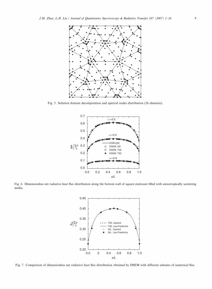
ARTICLE IN PRESS

Fig. 5. Solution domain decomposition and spectral nodes distribution (26 elements).

0.0 0.2 0.4 0.6 0.8 1.0

0.0

0.1

0.2

0.3

0.4

0.5

0.6

0.7

�=0.9

�=0.0

DOM [26]

DSEM, Q4

DSEM, T26

DSEM, T62

x/L

qw g�T

4

�=0.5

Fig. 6. Dimensionless net radiative heat flux distribution along the bottom wall of square enclosure filled with anisotropically scattering

media.

0.0 0 0.4 0.6 0.8 1.00.20

0.25

0.30

0.35

0.40

0.45

T26, Upwind

T26, Lax-Friedrichs

Q4, Upwind

Q4, Lax-Friedrichs

x/L

qw

�T4 g

Fig. 7. Comparison of dimensionless net radiative heat flux distribution obtained by DSEM with different schemes of numerical flux.

J.M. Zhao, L.H. Liu / Journal of Quantitative Spectroscopy & Radiative Transfer 107 (2007) 1–16 9

ARTICLE IN PRESS

0 1 2 3 4 5 6 7 8 9 1010-5

10-4

10-3

10-2

10-1

�L=10

�L=1.0

�L=0.1

Polynomial order, p

Inte

gra

l avera

ged r

ela

tive e

rror

�L=10

�L=1.0

�L=0.1

0 1 2 3 4 5 6 7 8 9 1010-4

10-3

10-2

10-1

Polynomial order, p

Inte

gra

l avera

ged r

ela

tive e

rror

Fig. 8. The p-convergence characteristics of the DSEM for solution with (a) quadrilateral elements (Q25) and (b) triangular elements

(T26).

R

0.4R

0.2R

o x

y

Fig. 9. Solution domain and mesh decomposition (535 elements) of the semicircular enclosure.


modeling schemes becomes unobservable from the figure. Figs. 8(a) and (b) show the p-convergencecharacteristics of the DSEM for solving the dimensionless net radiative heat flux of the bottom wall withquadrilateral (uniform 25 elements, Q25) and triangular elements (T26), respectively, for single scatteringalbedo o ¼ 0 and three different values of optical thickness, namely, tL ¼ 0.1, 1.0 and 10. The results obtainedusing the DSEM with 10th-order polynomial are considered as benchmark solution. Generally, the p-

convergence rates are fast for both quadrilateral and triangular elements. In the case with large values ofoptical thickness, namely, tL ¼ 10, the p-convergence rates follow exponential law.

3.3. Case 3: radiative transfer problem with angular discontinuity induced by shielding of interior obstacle

We consider radiative transfer in non-scattering media in a semicircular enclosure with a circular hole asshown in Fig. 9. The media is kept hot (1000K), while all other walls are black and kept cold (0K). As shownin Fig. 10, we consider the angular distribution of radiative intensity of a node denoted P at the bottom wall.The incident radiative energy of node P comes from three regions, namely regions A–C. Because the interiorcircular obstacle shields radiative energy of region D from reaching node P, the incident radiative energy ofnode P coming from region B is weaker than that coming from region A and C. As a result, the angulardistribution of radiative intensity of node P is remarkably non-uniform and contains discontinuity, thus theselected angular integration schemes should ensure that the radiative intensities coming from regions A–C

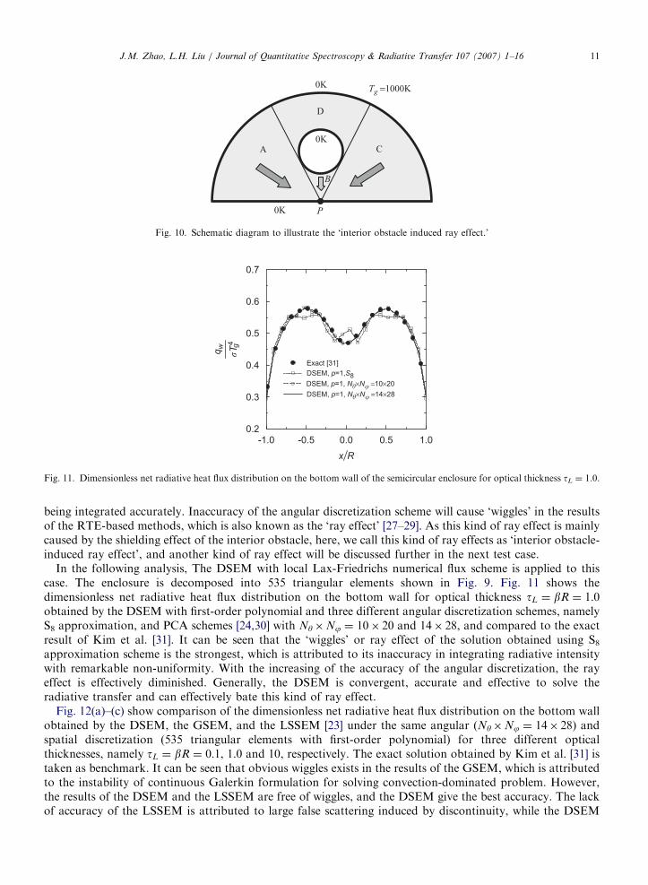
ARTICLE IN PRESS

B

0K

0K

P

Tg =1000K0K

A

D

C

Fig. 10. Schematic diagram to illustrate the ‘interior obstacle induced ray effect.’

-1.0 -0.5 0.0 0.5 1.00.2

0.3

0.4

0.5

0.6

0.7

Exact [31]

DSEM, p=1,S8

DSEM, p=1, N�×N� =14×28

DSEM, p=1, N�×N� =10×20

x R

qw g

�T4

Fig. 11. Dimensionless net radiative heat flux distribution on the bottom wall of the semicircular enclosure for optical thickness tL ¼ 1.0.


being integrated accurately. Inaccuracy of the angular discretization scheme will cause ‘wiggles’ in the resultsof the RTE-based methods, which is also known as the ‘ray effect’ [27–29]. As this kind of ray effect is mainlycaused by the shielding effect of the interior obstacle, here, we call this kind of ray effects as ‘interior obstacle-induced ray effect’, and another kind of ray effect will be discussed further in the next test case.

In the following analysis, The DSEM with local Lax-Friedrichs numerical flux scheme is applied to thiscase. The enclosure is decomposed into 535 triangular elements shown in Fig. 9. Fig. 11 shows thedimensionless net radiative heat flux distribution on the bottom wall for optical thickness tL ¼ bR ¼ 1:0obtained by the DSEM with first-order polynomial and three different angular discretization schemes, namelyS8 approximation, and PCA schemes [24,30] with Ny�Nj ¼ 10� 20 and 14� 28, and compared to the exactresult of Kim et al. [31]. It can be seen that the ‘wiggles’ or ray effect of the solution obtained using S8approximation scheme is the strongest, which is attributed to its inaccuracy in integrating radiative intensitywith remarkable non-uniformity. With the increasing of the accuracy of the angular discretization, the rayeffect is effectively diminished. Generally, the DSEM is convergent, accurate and effective to solve theradiative transfer and can effectively bate this kind of ray effect.

Fig. 12(a)–(c) show comparison of the dimensionless net radiative heat flux distribution on the bottom wallobtained by the DSEM, the GSEM, and the LSSEM [23] under the same angular (Ny�Nj ¼ 14� 28) andspatial discretization (535 triangular elements with first-order polynomial) for three different opticalthicknesses, namely tL ¼ bR ¼ 0:1, 1.0 and 10, respectively. The exact solution obtained by Kim et al. [31] istaken as benchmark. It can be seen that obvious wiggles exists in the results of the GSEM, which is attributedto the instability of continuous Galerkin formulation for solving convection-dominated problem. However,the results of the DSEM and the LSSEM are free of wiggles, and the DSEM give the best accuracy. The lackof accuracy of the LSSEM is attributed to large false scattering induced by discontinuity, while the DSEM

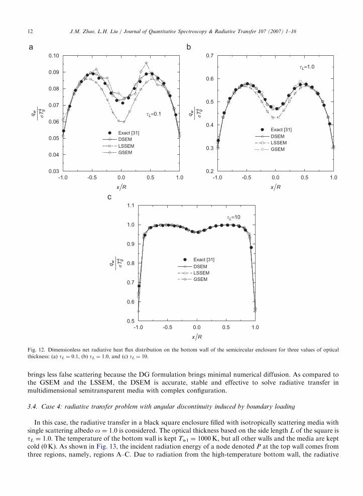
ARTICLE IN PRESS

-1.0 -0.5 0.0 0.5 1.00.03

0.04

0.05

0.06

0.07

0.08

0.09

0.10

�L=0.1

Exact [31]

DSEM

LSSEM

GSEM

x R

qw g

�T4

qw g

�T4

-1.0 -0.5 0.0 0.5 1.00.2

0.3

0.4

0.5

0.6

0.7

�L=1.0

Exact [31]

DSEM

LSSEM

GSEM

x R

x R

qw g

�T4

-1.0 -0.5 0.0 0.5 1.00.5

0.6

0.7

0.8

0.9

1.0

1.1

�L=10

Exact [31]

DSEM

LSSEM

GSEM

Fig. 12. Dimensionless net radiative heat flux distribution on the bottom wall of the semicircular enclosure for three values of optical

thickness: (a) tL ¼ 0.1, (b) tL ¼ 1.0, and (c) tL ¼ 10.


brings less false scattering because the DG formulation brings minimal numerical diffusion. As compared tothe GSEM and the LSSEM, the DSEM is accurate, stable and effective to solve radiative transfer inmultidimensional semitransparent media with complex configuration.

3.4. Case 4: radiative transfer problem with angular discontinuity induced by boundary loading

In this case, the radiative transfer in a black square enclosure filled with isotropically scattering media withsingle scattering albedo o ¼ 1.0 is considered. The optical thickness based on the side length L of the square istL ¼ 1.0. The temperature of the bottom wall is kept Tw1 ¼ 1000K, but all other walls and the media are keptcold (0K). As shown in Fig. 13, the incident radiation energy of a node denoted P at the top wall comes fromthree regions, namely, regions A–C. Due to radiation from the high-temperature bottom wall, the radiative

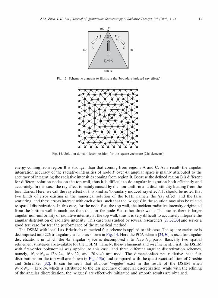
ARTICLE IN PRESS

1000K

0K0K

0K P

C

B

A

Tg=0K

ΔΩ

Fig. 13. Schematic diagram to illustrate the ‘boundary induced ray effect.’

Fig. 14. Solution domain decomposition for the square enclosure (226 elements).


energy coming from region B is stronger than that coming from regions A and C. As a result, the angularintegration accuracy of the radiative intensities of node P over 4p angular space is mainly attributed to theaccuracy of integrating the radiative intensities coming from region B. Because the defined region B is differentfor different solution nodes on the top wall, thus it is difficult to do angular integration both efficiently andaccurately. In this case, the ray effect is mainly caused by the non-uniform and discontinuity loading from theboundaries. Here, we call the ray effect of this kind as ‘boundary induced ray effect’. It should be noted thattwo kinds of error existing in the numerical solution of the RTE, namely the ‘ray effect’ and the falsescattering, and these errors interact with each other, such that the ‘wiggles’ in the solution may also be relatedto spatial discretization. In this case, for the node P at the top wall, the incident radiative intensity originatedfrom the bottom wall is much less than that for the node P at other three walls. This means there is largerangular non-uniformity of radiative intensity at the top wall, thus it is very difficult to accurately integrate theangular distribution of radiative intensity. This case was studied by several researchers [28,32,33] and serves agood test case for test the performance of the numerical method.

The DSEM with local Lax-Friedrichs numerical flux scheme is applied to this case. The square enclosure isdecomposed into 226 triangular elements as shown in Fig. 14. Here the PCA scheme [24,30] is used for angulardiscretization, in which the 4p angular space is decomposed into Ny�Nj parts. Basically two spatialrefinement strategies are available for the DSEM, namely, the h-refinement and p-refinement. First, the DSEMwith first-order polynomial was applied to this case, and three different angular discretization schemes,namely, Ny�Nj ¼ 12� 24, 16� 32, and 20� 40 are used. The dimensionless net radiative heat fluxdistributions on the top wall are shown in Fig. 15(a) and compared with the quasi-exact solution of Crosbieand Schrenker [32]. It can be seen that obvious ‘wiggles’ exist in the result of the DSEM whenNy�Nj ¼ 12� 24, which is attributed to the less accuracy of angular discretization, while with the refiningof the angular discretization, the ‘wiggles’ are effectively mitigated and smooth results are obtained.

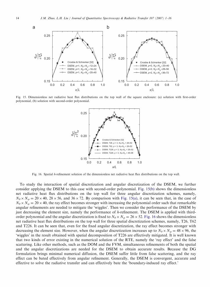
ARTICLE IN PRESS

0.0 0.2 0.4 0.6 0.8 1.00.15

0.20

0.25

Crosbie & Schrenker [32]

DSEM, p=1, N�×N�=20×40

DSEM, p=1, N�×N�=16×32

DSEM, p=1, N�×N�=12×24


DSEM, p=2, N�×N�=36×72

DSEM, p=2, N�×N�=28×56

DSEM, p=2, N�×N�=20×40

x L

0.0 0.2 0.4 0.6 0.8 1.00.15

0.20

0.25

x L

qw

1 w1

�T4

qw

1 w1

�T4

Fig. 15. Dimensionless net radiative heat flux distributions on the top wall of the square enclosure: (a) solution with first-order

polynomial, (b) solution with second-order polynomial.

0.0 0.2 0.4 0.6 0.8 1.00.15

0.20

0.25


DSEM, T26, p = 3, N�×N� = 26×52

DSEM, T62, p = 3, N�×N� = 26×52

DSEM, T226, p = 3, N�×N� = 26×52

DSEM, T226, p = 3, N�×N� = 48×96

x/L

qw

1

�T4 1w

Fig. 16. Spatial h-refinement solution of the dimensionless net radiative heat flux distributions on the top wall.


To study the interaction of spatial discretization and angular discretization of the DSEM, we furtherconsider applying the DSEM to this case with second-order polynomial. Fig. 15(b) shows the dimensionlessnet radiative heat flux distributions on the top wall for three angular discretization schemes, namely,Ny�Nj ¼ 20� 40, 28� 56, and 36� 72. By comparison with Fig. 15(a), it can be seen that, in the case ofNy�Nj ¼ 20� 40, the ray effect becomes stronger with increasing the polynomial order such that remarkableangular refinements are needed to mitigate the ‘wiggles’. Then we consider the performance of the DSEM byjust decreasing the element size, namely the performance of h-refinement. The DSEM is applied with third-order polynomial and the angular discretization is fixed to Ny�Nj ¼ 26� 52. Fig. 16 shows the dimensionlessnet radiative heat flux distributions on the top wall for three spatial discretization schemes, namely, T26, T62and T226. It can be seen that, even for the fixed angular discretization, the ray effect becomes stronger withdecreasing the element size. However, when the angular discretization increases up to Ny�Nj ¼ 48� 96, the‘wiggles’ in the result obtained with spatial decomposition of T226 are effectively mitigated. It is well knownthat two kinds of error existing in the numerical solution of the RTE, namely the ‘ray effect’ and the falsescattering. Like other methods, such as the DOM and the FVM, simultaneous refinements of both the spatialand the angular discretizations are needed for the DSEM to obtain accurate results. Because the DGformulation brings minimal numerical diffusion, the DSEM suffer little from false scattering, and the rayeffect can be bated effectively from angular refinement. Generally, the DSEM is convergent, accurate andeffective to solve the radiative transfer and can effectively bate the ‘boundary-induced ray effect.’


4. Conclusions

A discontinuous spectral element method (DSEM) is presented to solve radiative heat transfer inmultidimensional semitransparent media. This method is based on the general DG formulation, in whichChebyshev polynomial is used to build basis function on each element and both structured and unstructuredelements are considered. The DSEM have properties such as hp-convergence, local conservation and solutionsare allowed to be discontinuous across each element.

The DSEM with classical up-winding numerical flux scheme gives better results than the local Lax-Friedrichs numerical flux scheme on a coarse mesh while with mesh refining the difference between the resultsobtained through the two numerical flux modeling schemes becomes negligible. For the one-dimensional testcase, the p-convergence rates of DSEM are very fast and follow exponential law for different values ofextinction coefficient. For the two-dimensional test case, the p-convergence rates are fast for bothquadrilateral and triangular elements, and follow exponential law for large optical thickness.

Two kinds of ray effect of the RTE-based numerical methods, namely the boundary-induced ray effect andthe interior obstacle-induced ray effect, are studied. The DSEM brings less false scattering because the DGformulation brings minimal numerical diffusion, while the LSSEM suffers from large false scattering inducedby discontinuity. Like other methods, such as the DOM and the FVM, simultaneous refinements of both thespatial and the angular discretizations are needed for the DSEM to obtain accurate results. The DSEM isconvergent, accurate and effective to solve the radiative transfer problems in multidimensionalsemitransparent media with complex configuration and can effectively bate both the interior obstacle-induced ray effect and the boundary-induced ray effect.

Acknowledgments

The support of this work by the National Nature Science Foundation of China (50425619, 50336010) isgratefully acknowledged.

References

[1] Fiveland WA. Three-dimensional radiative heat-transfer solutions by the discrete-ordinates method. J Thermophys Heat Transfer

1988;2:309–16.

[2] Raithby GD, Chui EH. A finite-volume method for predicting a radiant heat transfer in enclosures with participating media. J Heat

Transfer 1990;112:415–23.

[3] Chai JC, Lee HS. Finite-volume method for radiation heat transfer. J Thermophys Heat Transfer 1994;8:419–25.

[4] Murthy JY, Mathur SR. Finite volume method for radiative heat transfer using unstructured meshes. J Thermophys Heat Transfer

1998;12:313–21.

[5] Kisslelev VB, Roberti L, Perona G. An application of the finite-element method to the solution of the radiative transfer equation.

JQSRT 1994;51:603–14.

[6] Liu LH. Finite element simulation of radiative heat transfer in absorbing and scattering media. J Thermophys Heat Transfer

2004;18:555–7.

[7] Howell JR, Perlmutter M. Monte Carlo solution of thermal transfer through radiant media between gray walls. J Heat Transfer

1964;86:116–22.

[8] Hottel HC, Cohen ES. Radiant heat exchange in a gas-filled enclosure allowance for nonuniformity of gas temperature. AIChE J

1958;4:3–14.

[9] Cui X, Li BQ. Discontinuous finite element solution of 2-D radiative transfer with and without axisymmetry. JQSRT

2005;96:383–407.

[10] Cui X, Li BQ. A discontinuous finite-element formulation for internal radiation problems. Numer Heat Transfer B 2004;46:223–42.

[11] Liu LH, Liu LJ. Discontinuous finite element method for radiative heat transfer in semitransparent graded index medium. JQSRT

2007;105:377–87.

[12] Bassi F, Rebay S. High-order accurate discontinuous finite element solution of the 2D Euler equations. J Comput Phys

1997;138:251–85.

[13] Cockburn B, Shu CW. The Runge–Kutta discontinuous Galerkin method for conservation laws v: multidimensional systems. J

Comput Phys 1998;141:199–224.

[14] Baumann CE, Oden JT. A discontinuous hp finite element method for convection–diffusion problems. Comput Methods Appl Mech

Eng 1999;175:311–41.


[15] Warburton TC, Karniadakis GE. A discontinuous Galerkin method for the viscous MHD equations. J Comput Phys

1999;152:608–41.

[16] Cockburn B. Discontinuous Galerkin methods. ZAMM 2003;83:731–54.

[17] Cockburn B, Karniadakis GE, Shu CW. The development of discontinuous Galerkin methods. In: Cockburn B, Karniadakis GE,

Shu CW, editors. Discontinuous Galerkin methods: theory, computation and applications. Berlin: Springer; 2000. p. 3–50.

[18] Patera AT. A spectral element method for fluid dynamics–laminar flow in a channel expansion. J Comput Phys 1984;54:468–88.

[19] Henderson RD, Karniadakis GE. Unstructured spectral element methods for simulation of turbulent flows. J Comput Phys

1995;122:191–217.

[20] Karniadakis GE, Sherwin SJ. Spectral/hp element methods for CFD. New York: Oxford University Press; 1999.

[21] Deville MO, Fischer PF, Mund EH. High-order methods for incompressible fluid flow. Cambridge: Cambridge University Press;

2002.

[22] Chai JC, Lee HS, Patankar SV. Finite-volume method for radiation heat transfer. In: Minkowycz WJ, Sparrow EM, editors.

Advances in numerical heat transfer, vol. 2. New York: Taylor & Francis; 2000. p. 109–41.

[23] Zhao JM, Liu LH. Least-squares spectral element method for radiative heat transfer in semitransparent media. Numer Heat Transfer

B 2006;50:473–89.

[24] Zhao JM, Liu LH. Solution of radiative heat transfer in graded index media by least square spectral element method. Int J Heat Mass

Transfer (2007), doi:10.1016/j.ijheatmasstransfer.2006.11.032.

[25] Zhao JM, Liu LH. Second order radiative transfer equation and its properties of numerical solution using finite element method.

Numer Heat Transfer B 2007;51:391–409.

[26] Kim TK, Lee H. Effect of anisotropic scattering on radiative heat transfer in two-dimensional rectangular enclosures. Int J Heat Mass

Transfer 1988;31:1711–21.

[27] Chai JC, Lee HS, Patankar SV. Ray effect and false scattering in the discrete ordinates method. Numer Heat Transfer B

1993;24:373–89.

[28] Ramankutty MA, Crosbie AL. Modified discrete ordinates solution of radiative transfer in two-dimensional rectangular enclosures.

JQSRT 1997;57:107–40.

[29] Coelho PJ. A modified version of the discrete ordinates method for radiative heat transfer modelling. Comput Mech 2004;33:375–88.

[30] Liu LH, Zhang L, Tan HP. Finite element method for radiation heat transfer in multi-dimensional graded index medium. JQSRT

2006;97:436–45.

[31] Kim MY, Baek SW, Park JH. Unstructured finite-volume method for radiative heat transfer in a complex two-dimensional geometry

with obstacles. Numer Heat Transfer B 2001;39:617–35.

[32] Crosbie AL, Schrenker RG. Radiative transfer in a two-dimensional rectangular medium exposed to diffuse radiation. JQSRT

1984;31:339–72.

[33] Larsen ME, Howell JR. The exchange factor method: an alternative zonal formulation of radiating enclosure analysis. J Heat

Transfer 1985;107:936–42.

dx.doi.org/10.1016/j.ijheatmasstransfer.2006.11.032

discontinuous spectral element method for solving...

Documents