discovering chasing behavior in moving object trajectories
TRANSCRIPT

JOBNAME: No Job Name PAGE: 1 SESS: 10 OUTPUT: Mon Aug 15 11:19:03 2011 SUM: 6FF0DCD3/v2451/blackwell/journals/tgis_v0_i0/tgis_1285
••
Discovering Chasing Behavior in MovingObject Trajectories
Fernando de LuccaSiqueira andVania Bogorny[fernandols, vania] @inf.ufsc.brDepartamento de Informatica eEstatisticaUFSC, Florianopolis, Brazil
AbstractWith the increasing use of mobile devices, a lot of tracks of movement of objects arebeing collected. The advanced trajectory data mining research has allowed thediscovery of many types of patterns from these data, like flocks, leadership, avoid-ance, frequent sequences, and other types of patterns. In this paper we introduce anew kind of pattern: a chasing behavior between trajectories. We present the maincharacteristics of chasing and propose a new method that extracts these new kind oftrajectory behavior pattern, considering time, distance, and speed as the mainthresholds. Experimental results show that our method finds patterns that not arediscovered by related approaches.
1 Introduction and Motivation
Modern tracking technology like GPS, cellphones and even sensor networks are beingheavily used in many different ways. This use produces spatio-temporal data that aretypically large and confused, and do not show/provide any visible information orknowledge. The spatio-temporal data generated by mobile devices, called trajectories ofmoving objects, provide characteristics of space and time, therefore making it possible toanalyze where something happened and when it happened. Trajectory data can beinteresting and useful in several application domains, like for instance, urban traffic,natural disasters, migration of birds and human mobility. For these applications, trajec-tory data can express different behaviors through space and time, e.g. move faster, changedirection, stand still, repeat the same route, etc.
The identification of different types of behaviors can help the user of an applicationto understand why something happened or what was the cause of certain actions. For
1
2
3
4
5
6
7
8
9
10
11
12
13
14
15
16
17
18
19
20
21
22
23
24
25
26
27
28
29
30
31
32
33
34
35
36
37
38
Transactions in GIS, 2011, ••(••): ••–••
© 2011 Blackwell Publishing Ltddoi: 10.1111/j.1467-9671.2011.01285.x
11
JOBNAME: No Job Name PAGE: 2 SESS: 10 OUTPUT: Mon Aug 15 11:19:03 2011 SUM: 4F9F0CFE/v2451/blackwell/journals/tgis_v0_i0/tgis_1285
instance, if an object follows the same route everyday and one day changes it, somethingcould have forced the change, such as a traffic jam. Or when in a large set of trajectoriesone object is avoiding a region, and this region is for instance a security camera, thisobject could be a thief. If in this case there has been a robbery in the same region, wecould find a suspect.
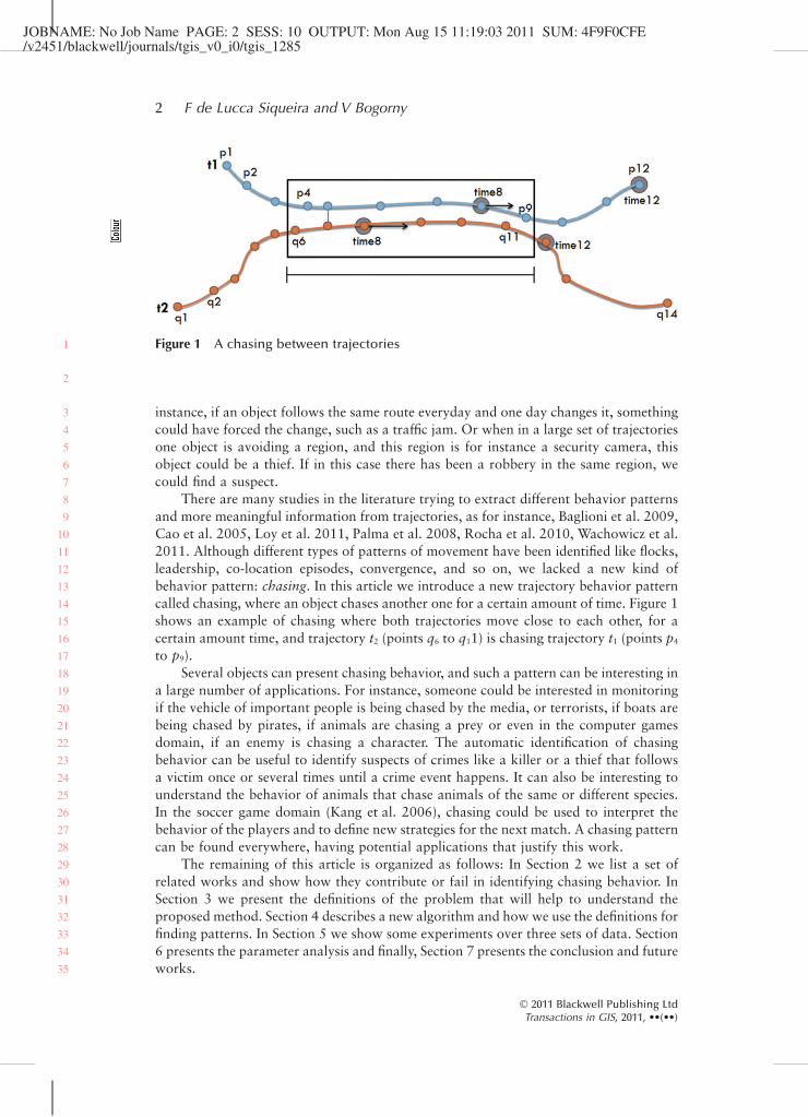
There are many studies in the literature trying to extract different behavior patternsand more meaningful information from trajectories, as for instance, Baglioni et al. 2009,Cao et al. 2005, Loy et al. 2011, Palma et al. 2008, Rocha et al. 2010, Wachowicz et al.2011. Although different types of patterns of movement have been identified like flocks,leadership, co-location episodes, convergence, and so on, we lacked a new kind ofbehavior pattern: chasing. In this article we introduce a new trajectory behavior patterncalled chasing, where an object chases another one for a certain amount of time. Figure 1shows an example of chasing where both trajectories move close to each other, for acertain amount time, and trajectory t2 (points q6 to q11) is chasing trajectory t1 (points p4
to p9).Several objects can present chasing behavior, and such a pattern can be interesting in
a large number of applications. For instance, someone could be interested in monitoringif the vehicle of important people is being chased by the media, or terrorists, if boats arebeing chased by pirates, if animals are chasing a prey or even in the computer gamesdomain, if an enemy is chasing a character. The automatic identification of chasingbehavior can be useful to identify suspects of crimes like a killer or a thief that followsa victim once or several times until a crime event happens. It can also be interesting tounderstand the behavior of animals that chase animals of the same or different species.In the soccer game domain (Kang et al. 2006), chasing could be used to interpret thebehavior of the players and to define new strategies for the next match. A chasing patterncan be found everywhere, having potential applications that justify this work.
The remaining of this article is organized as follows: In Section 2 we list a set ofrelated works and show how they contribute or fail in identifying chasing behavior. InSection 3 we present the definitions of the problem that will help to understand theproposed method. Section 4 describes a new algorithm and how we use the definitions forfinding patterns. In Section 5 we show some experiments over three sets of data. Section6 presents the parameter analysis and finally, Section 7 presents the conclusion and futureworks.
Figure 1 A chasing between trajectories1
2
3
4
5
6
7
8
9
10
11
12
13
14
15
16
17
18
19
20
21
22
23
24
25
26
27
28
29
30
31
32
33
34
35
2 F de Lucca Siqueira and V Bogorny
© 2011 Blackwell Publishing LtdTransactions in GIS, 2011, ••(••)

JOBNAME: No Job Name PAGE: 3 SESS: 10 OUTPUT: Mon Aug 15 11:19:03 2011 SUM: 648CB2A0/v2451/blackwell/journals/tgis_v0_i0/tgis_1285
2 Related Works
In this section we present some works that try to identify different types of patterns intrajectories. We can divide these works in three main groups.
The first group tries to identify patterns in groups of trajectories, where one tra-jectory is not aware of the other one, i.e., patterns are extracted among objects thatfollow the same path by coincidence, as in Gianotti et al. 2007, Lee et al. 2008,Hornsby and Cole 2007, Cao et al. 2009. The objective is to extract patterns amongobjects with similar movement, but without common intentional behavior. Giannottiproposed an algorithm to extract sequences of regions, frequently visited in a specifiedorder and with similar transition times. Trajectory patterns are generated as sequencesof regions visited by a minimal number of trajectories. Lee proposes a method toclassify sub-trajectories with different behaviors and different goals. Trajectories withthe same goal (discovered by the method) are added to the same group. For instance,ship trajectories that stop at a container port are classified into container ships, whiletrajectories that stop at a fishering area, for instance, are classified into fishing ships.Hornsby defines a model to represent groups of trajectories that have frequentsequences of events. Cao focuses on the frequent spatio-temporal sequential patternsproblem. As an object can use several routes to get to the same place, both thebeginning and the end of the trajectory must be the same to generate a sequentialpattern. It uses the direction, length, and distance to find similarity between parts oftrajectories.
The second group of works tries to identify patterns in single trajectories, trying tounderstand the behavior of the object by analyzing individual movements. Thietbohl, forinstance, uses the idea of stops and moves [19] to generate clusters (regions) with lowspeed, considered as the interesting places in trajectories. Loy addresses a new behaviorof trajectories, the avoidance. The objective is to find if a trajectory avoids a point, likea thief avoiding a surveillance camera. It also evaluates the confidence of the pattern, toensure that it was an intentional avoidance. Manso proposes an algorithm to find placesin single trajectories where the direction change characterizes the behavior, as forinstance a vessel in a fishing region. In [1], individual trajectories are enriched withsemantic information obtained from ontologies to infer the goal of the trajectory. Forexample, a trajectory that always starts at the same place (e.g. home) and stops every dayat the same place (e.g. work) is a worker trajectory. A trajectory that stops several timesat touristic places is a trajectory of a tourist.
The works presented in the two first groups formally define the patterns and proposealgorithms to extract the patterns from trajectories. There is a third group that defines aset of behaviors more conceptually. For instance, Laube et al. (2005) define five types oftrajectory behavior patterns: Convergence, Encounter, Recurrence, Flock and Leader-ship. Two patterns are closer to our work: Flock and Leadership. The Flock pattern refersto a group of objects that move in the same direction at the same time. It traces a circlearound a single object and searches for others inside this area that are moving in the samedirection at the same time. The Leadership pattern makes a small addition to the previousone: the leader object of the pattern must be moving in a certain direction, and after acertain amount of time, other objects near to the first one start to move into the samedirection as well. Both patterns use time, location, direction and distance to identify thesebehaviors, but neither the speed nor the length of the pattern is considered. The time isonly used to assure a minimum duration of the behavior.
1
2
3
4
5
6
7
8
9
10
11
12
13
14
15
16
17
18
19
20
21
22
23
24
25
26
27
28
29
30
31
32
33
34
35
36
37
38
39
40
41
42
43
44
45
46
47
48
Discovering Chasing Behavior in Moving Object Trajectories 3
© 2011 Blackwell Publishing LtdTransactions in GIS, 2011, ••(••)
2233
44
55

JOBNAME: No Job Name PAGE: 4 SESS: 10 OUTPUT: Mon Aug 15 11:19:03 2011 SUM: 689EFCD0/v2451/blackwell/journals/tgis_v0_i0/tgis_1285
Dodge et al. (2008) proposes a conceptual framework of movement and a taxonomyof movement patterns with their definitions. This work uses existing approaches, like theworks of Laube (2005) and Cao (2005), to define a set of measures to identify movementpatterns, like for instance, distance, speed, direction, etc. He divided movement patternsin two groups: generic patterns and behavioral patterns. The main difference is thatbehavioral patterns are context-dependent, as for instance, the common movement ofcertain animal species. One of the defined behavioral patterns was pursuit/evasion, whichrefers to an animal trying to escape from a predator where both trajectories havehigh-speed movements and several turnings. Dodge only describes the movement pat-terns and the associated measures, without providing any formal definition or algorithmspecific for finding chasing, which is the proposal of this article. Legendre et al. (2006)proposed a new modeling approach to mobility data. This work defines motions ofobjects with behavioral rules, where one object should have a certain behavior dependingon a certain context. For example, the individual walk of an object in a certain contextshould follow some rules like avoid walls, avoid obstacles and avoid other objects. Achasing behavior is also defined, where one object moves in direction to another objector to a static point, but neither time nor distance is considered for really identifying if anobject chases another one for a certain time.
In Hornsby and King (2008) a set of motion relations between vehicles on roadnetwork is presented. These relations, isBehind, inFrontOf, driveBeside and passBy,describe the relative position between two vehicles in a particular time, as for instance,if one vehicle is in front or behind the other. A chasing could be interpreted as the objectthat is behind a target for a certain amount of time. However, the relationship is definedonly for a specific timestamp, not for a time interval, and only when one object is exactlybehind the other, with the same timestamp. Indeed, no duration is taken into account todiscover for how long the relation holds, and also if the object is not exactly behind theother, no chasing is characterized.
Reynolds (1999) addresses the problem of autonomous characters, movement in avirtual world. He defines a set of actions and movements, like seek, pursuit, flee andwander, that together model the steering behavior. The main objective is to set a path tobe followed by the character given a certain goal as, for example, to follow a corridoravoiding obstacles. The pursuit behavior characterizes a chase, but differently from ourproposal, the objective is to define a path to be followed by an object in real time. Ourproposal is to find chasing behavior thorough the analysis of past trajectories, and not todefine the route of an object.
Wachowicz (2011) extended the work of Laube, and proposed an algorithm to findflocks between objects that must be moving together during a certain amount of time. Inthis approach the objects may not stand without moving. In this approach the directionis not considered. Apart from this, the main problem is that the moving objects mustremain in flocks at exactly the same timestamps, which is not exactly the case for chasing.
Cao et al. (2006) explore the collocation episodes in spatio-temporal data. Forexample, a puma hunting a dear. The main objective is to find objects that move togetherfor a certain amount of time and make another object move with them. Therefore, theconcept of time window is used, where trajectories are divided in time slices, and theneach slice is evaluated to discover an episode. The relationship between objects isidentified through the distance between points in each time window. The time is used toassure a minimum time duration and for the time window, but also to find a pattern arequirement is that trajectories must have the same timestamps inside the time window.
1
2
3
4
5
6
7
8
9
10
11
12
13
14
15
16
17
18
19
20
21
22
23
24
25
26
27
28
29
30
31
32
33
34
35
36
37
38
39
40
41
42
43
44
45
46
47
48
4 F de Lucca Siqueira and V Bogorny
© 2011 Blackwell Publishing LtdTransactions in GIS, 2011, ••(••)
66 7

JOBNAME: No Job Name PAGE: 5 SESS: 10 OUTPUT: Mon Aug 15 11:19:03 2011 SUM: 4B7A37BA/v2451/blackwell/journals/tgis_v0_i0/tgis_1285
This restriction limits the method when trajectories were collected at time intervals whichwere similar but not identical, but not and also when the trajectories were collected withdifferent time intervals (e.g. a trajectory collected every 1 second and another every 2 ormore seconds).
Finding chasing patterns in trajectories is not the objective of Cao et al. Althoughdistance and time are considered to Þnd objects that are close in space, the way it usesthese parameters is not enough to characterize chasing.
Previous works could somehow be used to identify chasing patterns, but none ofthem considered sufÞcient characteristics for really identifying it. While most previousworks deal with groups of trajectories or simply identify patterns in the trajectory of oneindividual, here we work with pairs of trajectories, and discover the behavior of oneobject in relation to another one.
3 Basic Concepts and DeÞnitions
A chasing pattern has some special characteristics that deÞne its behavior. In this sectionwe discuss some deÞnitions that will help the reader to understand this new kind ofpattern and our algorithm.
DeÞnition 1. Trajectory. A trajectory T is a list of space-time points�tid , p0,p1, . . . , pn�, where pi = (xi, yi, ti) and xi, yi, ti � R for i = 0, . . . , n and t0 < t1
< . . . < tn. Every T is identiÞed by a trajectory identiÞer calledtid .
Because a trajectory chasing pattern may not exist in the whole trajectory, wepartition a trajectory into sub-trajectories.
DeÞnition 2. sub-trajectory. A sub-trajectory S of T = �p0, p1, p2, . . . , pn�is a list of space-time points �pi, pi+1, . . . , pi+m,�, where pi ( T and 0 � i �m + i � n.
A chasing does not occur between trajectories of different days or with a large timeinterval. To avoid the comparison of trajectories collected with long time differences, weintroduce the concept of time tolerance. A time toleranceDt is a maximum time intervalbetween two trajectories that ensures that they happened in a near/similar time period.If two trajectories are in the same time period we say that they are acandidate chasing.
DeÞnition 3. Candidate Chasing. Let S1 = �p0, p1, . . . , pn� and S2 = �q0,q1, . . . , qm� be sub-trajectories of T1 and T2, respectively. S1 and S2 respectthe time tolerance Dt if and only if S2 |tp0 - tq0| � Dt and |tpn - tqm| � Dt andtqm > tpn.
Figure 2 shows an example of deÞnition 3. Let us considerDt as 0:05, the pair (S1,S2) is a candidate chasing becausep1t = 1:00 at S1 andq1t = 1:04 at S2, so |p1t - q1t| � Dt� |1:00 - 1:04| � 0:05 and p2t = 1:05 at S1 andq2t = 1:08 at S2, so |p2t - q2t| � Dt � |1:05- 1:08| � 0:05.
To reduce the number of points of a sub-trajectory, we build a line segment betweenthe Þrst and the last point of the sub-trajectory, that we callrepresentative line segment.
1
2
3
4
5
6
7
8
9
10
11
12
13
14
15
16
17
18
19
20
21
22
23
24
25
26
27
28
29
30
31
32
33
34
35
36
37
38
39
40
41
42
43
44
45
46
Discovering Chasing Behavior in Moving Object Trajectories 5
© 2011 Blackwell Publishing LtdTransactions in GIS, 2011, ••(••)
88
JOBNAME: No Job Name PAGE: 6 SESS: 10 OUTPUT: Mon Aug 15 11:19:03 2011 SUM: 38355FE7/v2451/blackwell/journals/tgis_v0_i0/tgis_1285
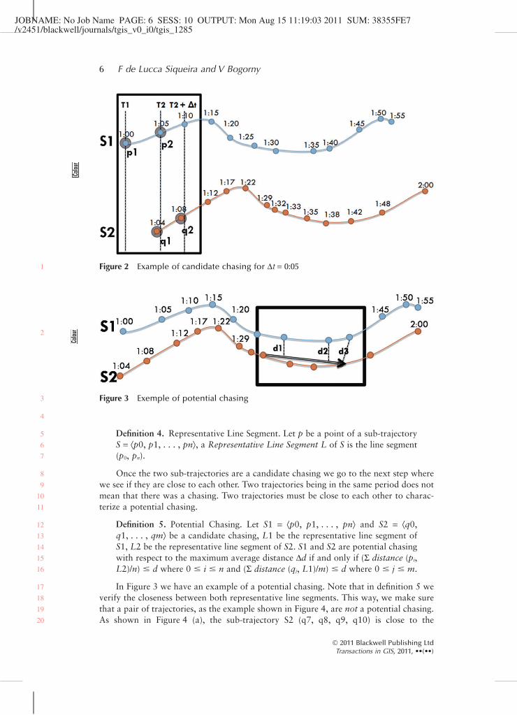
Definition 4. Representative Line Segment. Let p be a point of a sub-trajectoryS = ⟨p0, p1, . . . , pn⟩, a Representative Line Segment L of S is the line segment(p0, pn).
Once the two sub-trajectories are a candidate chasing we go to the next step wherewe see if they are close to each other. Two trajectories being in the same period does notmean that there was a chasing. Two trajectories must be close to each other to charac-terize a potential chasing.
Definition 5. Potential Chasing. Let S1 = ⟨p0, p1, . . . , pn⟩ and S2 = ⟨q0,q1, . . . , qm⟩ be a candidate chasing, L1 be the representative line segment ofS1, L2 be the representative line segment of S2. S1 and S2 are potential chasingwith respect to the maximum average distance Dd if and only if (S distance (pi,L2)/n) � d where 0 � i � n and (S distance (qj, L1)/m) � d where 0 � j � m.
In Figure 3 we have an example of a potential chasing. Note that in definition 5 weverify the closeness between both representative line segments. This way, we make surethat a pair of trajectories, as the example shown in Figure 4, are not a potential chasing.As shown in Figure 4 (a), the sub-trajectory S2 (q7, q8, q9, q10) is close to the
Figure 2 Example of candidate chasing for Dt = 0:05
Figure 3 Exemple of potential chasing
1
2
3
4
5
6
7
8
9
10
11
12
13
14
15
16
17
18
19
20
6 F de Lucca Siqueira and V Bogorny
© 2011 Blackwell Publishing LtdTransactions in GIS, 2011, ••(••)

JOBNAME: No Job Name PAGE: 7 SESS: 10 OUTPUT: Mon Aug 15 11:19:03 2011 SUM: 3140F0F9/v2451/blackwell/journals/tgis_v0_i0/tgis_1285
representative line L1 (p5, p8) of S1. But when we compare the distance betweensub-trajectory S1 (p5, p6, p7, and p8) in Figure 4 (b), with the line segment L2 (q7, q10),the minimal distance threshold is not satisfied, so not characterizing a potential chasingin this case.
In some applications the speed can also indicate a chasing. When an object is chasinganother one, their average speed must be similar, or one object will move far away fromthe other. This can occur in some types of chasing like a thief chasing a victim or a policechasing a suspect. In this article we consider the speed as an optional factor, and evaluatechasing with and without using speed.
Definition 6. Speed. Let S1 and S2 be a potential chasing, Da1 and Da2 be theaverage speed of S1 and S2, respectively, and a be the maximum percentagedifference between speeds, both sub-trajectories will have the same averagespeed if (1 - a) � (Da1/Da2) � (1 + a) with a ( [0,1]
Notice that to find a chasing considering speed, the speed of both trajectories can beeither high or low. What matters is that the speed must be similar.
With these definitions we can finally define a chasing behavior:
Definition 7. Sub-Chasing. Let S1 and S2 be two candidate chasing trajectorieswith respect to a time tolerance Dt, if S1 and S2 are a potential chasing, we havea sub-chasing where S2 is chasing S1.
Figure 4 (a) potential chasing is detected and (b) potential chasing is not confirmed1
2
3
4
5
6
7
8
9
10
11
12
13
14
15
16
17
18
19
20
21
Discovering Chasing Behavior in Moving Object Trajectories 7
© 2011 Blackwell Publishing LtdTransactions in GIS, 2011, ••(••)

JOBNAME: No Job Name PAGE: 8 SESS: 10 OUTPUT: Mon Aug 15 11:19:03 2011 SUM: 4E80E0F9/v2451/blackwell/journals/tgis_v0_i0/tgis_1285
To have a chasing pattern we need two trajectories: One being chased and anotherchasing. We name the first one as target, because it is the target of the chasing, and thesecond as stalker, because it is chasing the target.
Definition 8. Pure-Chasing. A trajectory T1 named as target is being chased bya trajectory T2, named stalker, if S duration of the set of sub-chasing betweenT1 and T2 is greater then a minimum time duration Dc.
In others words, a chasing pattern is detected when two trajectories remain close toeach other for a period of time and respecting a time tolerance.
Definition 9. Speed-Chasing. A trajectory T1 named as target is being chased bya trajectory T2, named stalker, if S duration of the set of sub-chasing betweenT1 and T2 is greater then a minimum time duration Dc and the average speedof T1 is the same as T2.
Based on the above definitions we can finally define an algorithm to find chasingpatterns, which is presented in the following section.
4 TRA-CHASE: An Algorithm to Identify Trajectory Chasing Patterns
In this section we present an algorithm to identify trajectory chasing patterns, namedTRA-CHASE. In general words, this algorithm, shown in listing 1.1, tries to identifysub-trajectories that contain a chasing pattern. The part that identifies sub-trajectorieswith a chasing pattern is presented in the SUB-CHASE procedure, shown in listing 1.3.The set of sub-chases identified between two trajectories will result in the TRA-CHASEpattern.
The TRA-CHASE algorithm takes as input a set of trajectories T of different objects,the minimum time duration of the pattern Dc, the time tolerance Dt and the maximumallowed distance Dd between trajectories that characterizes a chasing. The speed param-eter is a flag that tells the algorithm if it should either consider speed or not for computingchasing patterns.
For each pair of different trajectories (lines 12, 13, 15), the algorithm analyses everysub-trajectory (lines 22 an 30) to find if there are two sub-trajectories having a chasingpattern. Then, the algorithm moves to the next step until it covers the completetrajectory.
The first step is to create the sub-trajectories P1 and P2 (lines 17 and 19), with thetwo initial points of trajectories t1 and t2, respectively. Having these two points P1 andP2, the algorithm generates sub-trajectories S1 and S2 (lines 20 and 21) with the methodGETsub-trajectory (shown in listing 1.2). The objective of this step is to optimize thealgorithm, avoinding point to point comparison of both trajectories. The next step is toidentify chasing behavior between the sub-trajectories S1 and S2 (line 22). If a sub-chasing is found between the sub-trajectories, both S1 and S2 are added to the set ofchasing patterns C (line 24), and the algorithm jumps to the timestamps of t1 and t2(lines 25 and 27) that correspond to the final timestamps of S1 and S2, respectively.
In case no sub-chasing is found between S1 and S2, then we have to test point bypoint, and the algorithm searches for a pattern between P1 and P2 (line 30). If there isa pattern between P1 and P2 (line 32) it is added to C (line 32), and the algorithm jumps
1
2
3
4
5
6
7
8
9
10
11
12
13
14
15
16
17
18
19
20
21
22
23
24
25
26
27
28
29
30
31
32
33
34
35
36
37
38
39
40
41
42
43
44
8 F de Lucca Siqueira and V Bogorny
© 2011 Blackwell Publishing LtdTransactions in GIS, 2011, ••(••)

JOBNAME: No Job Name PAGE: 9 SESS: 10 OUTPUT: Mon Aug 15 11:19:03 2011 SUM: 285E00B5/v2451/blackwell/journals/tgis_v0_i0/tgis_1285
to the next point of t1 and t2 (lines 33 and 34) and starts the process again. In case nochasing behavior is found between P1 and P2 the algorithm moves to the next point oft2 (line 36), looking for a sub-trajectory of t2 that may have a chasing with the currentsub-trajectory of t1. Finally, if no sub-trajectories of t2 have chasing behavior with thecurrent sub-trajectory of t1, the algorithm moves to the next point of t1 (line 38), and theprocess starts again.
At the end, if the duration of the subchases is higher than the minimum duration Dd(line 40), the chasing pattern C is added to the set of chasing patterns chasingSet (line 41).The chasing pattern is two lists of points, one from the target that was being chased andthe other from the stalker that chased the target.
Listing 1.2 shows the pseudo-code of the method that generates sub-trajectories,grouping them by time. This method has as input a pair of points P of the trajectory t andthe time tolerance Dt. The output is a sub-trajectory S. First, the algorithm takes the lastpoint of P (line 8) called q. Then the algorithm goes to the point after q (line 10) andchecks if the timestamp of each consecutive point is lower than the timestamp of q plus
1
2
3
4
5
6
7
8
9
10
11
12
13
14
15
Discovering Chasing Behavior in Moving Object Trajectories 9
© 2011 Blackwell Publishing LtdTransactions in GIS, 2011, ••(••)

JOBNAME: No Job Name PAGE: 10 SESS: 10 OUTPUT: Mon Aug 15 11:19:03 2011 SUM: 1EE1A26F/v2451/blackwell/journals/tgis_v0_i0/tgis_1285
Dt/2 (line 12).n. We group the points by time to overcome the problem when differenttrajectories are generated with different time intervals. By grouping points to generatesub-trajectories using just the number of points instead of time, we could generatesub-trajectories without chasing characteristics.
To compute the sub-trajectory, first, we have to confirm that both sub-trajectories arein the same time period. So in the SUB-CHASE procedure, presented in listing 1.3, we test(line 13) the time tolerance and find the candidate chasing. In this step we test if the
1
2
3
4
5
6
7
10 F de Lucca Siqueira and V Bogorny
© 2011 Blackwell Publishing LtdTransactions in GIS, 2011, ••(••)

JOBNAME: No Job Name PAGE: 11 SESS: 10 OUTPUT: Mon Aug 15 11:19:03 2011 SUM: 5E1EC52B/v2451/blackwell/journals/tgis_v0_i0/tgis_1285
sub-trajectory S2 has its ending time before the ending time of S1 plus the time tolerance.It means that the trajectory of the stalker must have happened after the target. Forexample, if the target passes by a local X at time t1, the stalker has to pass around localX at a time t2 where t2 � t1. This step prevents comparing two trajectories from differentdays or with long time difference.
Only if S2 respects the time tolerance do we go to the next step, which analyzes thedistance as in definition 5 (line 14), to check if the subchase is a potential chasing. Thestalker cannot always act the same way as the target, but he always tries to be close tothe target. The stalker can change its behavior over the sub-trajectory, being closer orfarther from the target. Therefore, the algorithm uses the average distance to evaluate ifboth objects remained close. If the average distance between them is less than Dd, thenboth sub-trajectories are close to each other.
Another matter is the order of the objects. In a regular chasing, the target will alwaysbe in front of the stalker, because the stalker must see where the target is heading. Thisis checked in line 15 of the sub-chase procedure in 1.3.
An important remark is that, in case the roles of the chasing invert, i.e. the targetbecomes the stalker and the stalker becomes the target, the algorithm will find a newchasing pattern, different from the previous one.
The last analyzed property is the speed (line 17). Sometimes even if two trajectoriesmove together for a certain amount of time, they should move around the same speed.If the target is moving faster then the stalker and the target is moving away, it means thatthe stalker did not intend to pursue the target, because he did not keep the target ontrack. On the other hand, if the stalker is moving faster than the target, he will pass thetarget and keep moving. Based on our definition 6 we check if both sub-trajectories havethe same average speed during the same time period. We decide a maximum limit of 20%of difference between the trajectories speed. We considered that if an object is trying toadjust its speed with another one, and a 20% of difference should be a good value tocontrol the distance between them.
Since the speed is optional, we evaluate the algorithm with and without using speed,calling the comparisons as Pure – Chase and Speed – Chase, as in the previous definitions.
5 Experimental Results
To evaluate the proposed algorithm we considered three datasets. The first one, shown inFigure 5, was synthetically generated by the Knowledge Discovery and Data Miningresearch unit to simulate a flock pattern. In this dataset several objects move together ata certain time. The objective of using this dataset is to find chasing patterns among flocks,and to show that we find chasing patterns that are not discovered by the flock algorithm.
The second dataset is from a mobile learning game developed by the Waag Society,in the Netherlands. It is a city game with GPS and mobile phones with students aged 12to 14. The game consists of various geo-referenced places associated with multimediariddles and questions. The player receives a historical map with checkpoints and has therole to find these places in the real life. The 466 students were divided in six groups andthe game took place in 2005 from 7 to 9 February. In this dataset we try to find chasingbehavior between students of different groups. If someone did not discover the riddle anddid not know where to go, he can try to follow someone of another group who decryptedthe puzzle, therefore characterizing a chasing.
1
2
3
4
5
6
7
8
9
10
11
12
13
14
15
16
17
18
19
20
21
22
23
24
25
26
27
28
29
30
31
32
33
34
35
36
37
38
39
40
41
42
43
44
45
46
47
Discovering Chasing Behavior in Moving Object Trajectories 11
© 2011 Blackwell Publishing LtdTransactions in GIS, 2011, ••(••)

JOBNAME: No Job Name PAGE: 12 SESS: 10 OUTPUT: Mon Aug 15 11:19:03 2011 SUM: 342E3DEB/v2451/blackwell/journals/tgis_v0_i0/tgis_1285
In the third dataset we captured data of a group of people walking with a GPS deviceat Jurere Internacional beach, located in Florianopolis, Brazil. Differently from theprevious dataset, GPS devices produce data that can be diffuse and not linear. In thisdataset, the target walked for around 1 hour and a group of 5 possible stalkers walkedat different times simulating some chasing behaviors. In this dataset we know who is thetarget, who are the stalkers, when and where the chasing occurs. The points of the targetwere captured every 2 seconds and the points of the stalker each 1 second, so we showthat our method works very well with trajectories collected at different time intervals.
We compare our algorithm with two others: the Moving Flock Finder (MFF)(Wachowicz et al. 2011, Knowledge Discovery and Data Mining Research unit 2011),[4]) and the Collocation Discovery Algorithm (CDA) (Cao et al. 2006). We run ouralgorithm PURE TRA-CHASE(PTC) and SPEED TRA-CHASE(STC).
The code was written in java, the data were stored in a postgres database extendedwith postgis, and we used the software Quantum GIS to visualize the results.
5.1 Experiments with Dataset 1
In this first experiment we used a subset of 17 trajectories. We run all four algorithmswith the same parameters. All of them with the same distance Dd = 80.0 m, durationDc = 10 min and the time tolerance Dt = 5 min. We defined 80 meters as the minimundistance because the average distance between the points of a trajectory in this syntheticdataset varies between 40 meters and 160 meters in a time interval of around one minute.The time window parameter for CDA should have the same value as our time tolerance.
Figure 5 Trajectories of the first dataset1
2
3
4
5
6
7
8
9
10
11
12
13
14
15
16
17
18
19
20
21
22
23
24
12 F de Lucca Siqueira and V Bogorny
© 2011 Blackwell Publishing LtdTransactions in GIS, 2011, ••(••)

JOBNAME: No Job Name PAGE: 13 SESS: 10 OUTPUT: Mon Aug 15 11:19:03 2011 SUM: 6A7146F3/v2451/blackwell/journals/tgis_v0_i0/tgis_1285
In this experiment, the flock algorithm (MFF) found one pattern, the co-location(CDA) found two, PTC found six and STC found four patterns, as shown in Table 1.Both MFF and CDA found the same pattern, but since CDA does not differ which objectis in front of the other, it found the same pattern twice. The PTC (considering speed)found more patterns then the others, once it does not consider the speed betweentrajectories. The patterns found by STC were also found by PTC, but they were shorterbecause the sub-trajectories did not had the same speed.
Figure 6 shows two sub-trajectories S1 and S2 to explain why CDA does not find achasing that the Pure-chasing or the Speed-chasing find. CDA compares the points withsame timestamp, so it compares the points q2 and q3 of sub-trajetory S2 with the pointsp5 and p6 of sub-trajectory S1, as shown in Figure 6 (a). These points are far from eachother, so not respecting the minimal distance. On the other hand, our method PTCcompares all points between q2 and q6 of sub-trajectory S2 with the points p5 and p6 ofthe sub-trajectory S1, as shown in Figure 6 (b). Notice that the areas that cover the pointsbetween the sub-trajectories intersect each other, therefore characterizing a chasingpattern.
What we can conclude in this experiment is that the way time is used by the methodmakes the difference in the discovered patterns.
5.2 Experiments with Dataset 2
In this dataset the objective was to find chasing patterns between individuals of differentgroups, assuming that if someone does not know where to go, he/she might want to chasesomeone who knows the next place.
Among the three datasets, this was the largest and more complex. Each trajectoryhas several points with different time intervals. In the same trajectory, two consecutivespoints could have from 1 to 60 seconds of difference.
Since the flock algorithm MFF cannot work with data captured at different timeintervals, we ran a synchronizer software from Wachowicz et al. (2011) to try to findflock patterns. After analysing the data we ran the four algorithms with both thesyncronized data and the original data, with the parameters Dt = [1 minute and 3minutes] (time needed for one trajectory to catch the other), Dd = [15 meters and 30meters] and Dc = 10 minutes. The results are shown in Tables 2 and 3.
Even with the synchronized data and considering two different values for both timetolerance and distance, the MFF did not find any pattern. The CDA found many fewerpatterns then our method. Both PTC and STC found almost the same patterns, showing
Table 1 Comparison of the duration of the patterns found by the different algorithmsconsidering Dd = 80.0 m for PTC, STC, CDA and MFF
Pattern PTC STC CDA MFF
C1 18:23–19:50 18:25–19:50 18:27–19:47 18:26–19:45C2 18:16–18:55 18:16–18:49 – –C3 18:18–18:35 18:18–18:34 – –C4 20:11–20:21 – – –C5 18:18–18:32 18:18–18:28 – –C6 18:23–19:50 18:23–19:50 – –
1
2
3
4
5
6
7
8
9
10
11
12
13
14
15
16
17
18
19
20
21
22
23
24
25
26
27
28
29
30
31
32
33
34
35
36
37
38
39
40
41
42
43
44
45
46
47
Discovering Chasing Behavior in Moving Object Trajectories 13
© 2011 Blackwell Publishing LtdTransactions in GIS, 2011, ••(••)

JOBNAME: No Job Name PAGE: 14 SESS: 10 OUTPUT: Mon Aug 15 11:19:03 2011 SUM: 3438A0E2/v2451/blackwell/journals/tgis_v0_i0/tgis_1285
that the speed of the trajectories was very similar. As can be seen in Tables 2 and 3, andas was expected, by synchronizing the data, the co-location algorithm (CDA) found morepatterns than with the original data. The same occurs with our methods, but our twoalgorithms always find more chasing patterns. In summary, all approaches found morepatterns on the synchronized data.
Figure 6 (a) Points compared in CDA and MFF and (b) points compared by PTC and STC
Table 2 Number of patterns found by PTC, STC, CDA and MFF with the syncronizeddata
Test PTC STC CDA MFF
Dd = 15 m Dt = 1 minute 105 101 64 0Dd = 15 m Dt = 3 minutes 152 148 33 0Dd = 30 m Dt = 1 minutes 244 240 180 0Dd = 30 m Dt = 3 minutes 297 297 72 0
1
2
3
4
5
6
7
8
9
10
11
12
13
14
15
16
17
14 F de Lucca Siqueira and V Bogorny
© 2011 Blackwell Publishing LtdTransactions in GIS, 2011, ••(••)

JOBNAME: No Job Name PAGE: 15 SESS: 10 OUTPUT: Mon Aug 15 11:19:03 2011 SUM: 4AE02451/v2451/blackwell/journals/tgis_v0_i0/tgis_1285
Although there were many chasing patterns, this occurred because most patternswere found in regions where the students stoped moving, or moved slowly. These regionsrepresent either the historical places (where the students were answering the riddles) orwhere the students were resting. As the points in these regions are very close, thealgorithms CDA, PTC and STC found the same patterns. This kind of patterns locatedin dense regions of points, as can be seen in Figure 7, is the only kind of pattern foundby CDA. CDA misses any pattern on the path between regions, while our method foundchasing patterns on the path between the regions, as shown in Figure 8.
Figure 8 shows a more interesting kind of pattern that is only found by our method.There are two trajectories moving from region A to region B. The PTC identifies this asa chasing C. A student, after answered the riddles, walks to the next historical placefollowed by another student.
Table 3 Number of patterns found by PTC, STC, CDA and MFF with the original data
Test PTC STC CDA MFF
Dd = 15 m Dt = 1 minute 93 90 11 0Dd = 15 m Dt = 3 minutes 139 136 4 0Dd = 30 m Dt = 1 minutes 169 167 36 0Dd = 30 m Dt = 3 minutes 217 215 27 0
Figure 7 Pattern found by PTC, STC and CDA for Dd = 15 m Dt = 1 minute
Figure 8 Pattern found by PTC and STC for Dd = 15 m Dt = 1 minute
1
2
3
4
5
6
7
8
9
10
11
12
13
14
15
16
17
18
19
20
21
22
23
24
25
Discovering Chasing Behavior in Moving Object Trajectories 15
© 2011 Blackwell Publishing LtdTransactions in GIS, 2011, ••(••)

JOBNAME: No Job Name PAGE: 16 SESS: 10 OUTPUT: Mon Aug 15 11:19:03 2011 SUM: 5CA074F5/v2451/blackwell/journals/tgis_v0_i0/tgis_1285
5.3 Experiments with Dataset 3
In this dataset we know where each chasing starts and finishes, so we can better evaluatethe results. We ran the algorithms with distance Dd = 10 m, duration Dc = 3 min and timetolerance Dt = 30 seconds. In pedestrian chasing, 10 meters is an acceptable distance foran object to keep another one under his/her eyes, avoiding being too close. As the timeinterval between the collected points was 1 second and 2 seconds, where pedestrianswalked in low velocity, we considered that 30 seconds for time tolerance is a goodmeasure for an object to be 10 meters behind the other.
This dataset has 5 chasing patterns, where object 0 was chased by objects 1 and 2once, and by objects 3 and 5 twice. In this experiment, PTC found 6 patterns and STCfound the 5 original patterns. Note that these are short trajectories, with duration around20 to 30 minutes, so the chasing patterns are short too.
Both flock (MFF) and co-location (CDA) algorithms did not find any pattern. Thenwe ran the experiment with different parameters, and still did not get any instance ofpattern from MFF. The algorithm CDA found 3 patterns only when we set Dd = 25 m.A comparison of the results is shown in Table 4. By looking at the first row in the table,the pattern C1 represents the original pattern (real duration). Our two algorithms foundalmost the real pattern. On the other hand, CDA found a pattern before the originalchasing.
Figure 9 shows a comparison of the pattern C1 generated by CDA and our algo-rithms (STC and PTC). Notice that the pattern found by CDA is before the real chasing.For all other patterns, represented in Table 4, our methods (STC and PTC) foundpatterns very similar to the original ones. The flock algorithm did not find patterns, andCDA found two patterns similar to the original ones (pattern C4a and C4b).
6 Parameter Analysis and Discurssion
An important matter is how to set the appropriate parameters. This is a general problemfor most data mining algorithms. One can make several tests until finding the bestparameters, and this has a cost and may change from one application to another.
The main contribution of our work is the way that we use the time dimension (timetolerance). The value of the time tolerance should be based on how much time the stalkertakes to cross the same region as its target. For instance, in Figure 10 the target S1entered the region X at time 1:35 and the stalker S2 entered at time 1:50. So the timetolerance in this case should be at least 0:15 in order to the sub-trajectory S1 at time 1:35be comparable with the sub-trajectory S2 at time 1:50.
As the co-location and flock algorithms use the distance to define closeness at thesame timestamp, it may occur that at the same time two sub-trajectories are far from eachother. As we use the time tolerance to compare closeness between two sub-trajectoriesfixing the timestamp of the target and move ahead in time of the stalker, our method findsthat two objects are close to each other at different timestamps, therefore characterizinga chasing. An example is given in Figure 10, where existing works would compare thedistance between points p5 of S1 and q2 of S2 with a distance d1, while our methodwould compare point p5 of S1 with q5 of S2, therefore having a distance of d2. Insummary, as our method compares one timestamp of the target with several timestampsof the stalker, respecting Dt, we find more realistic chasing.
1
2
3
4
5
6
7
8
9
10
11
12
13
14
15
16
17
18
19
20
21
22
23
24
25
26
27
28
29
30
31
32
33
34
35
36
37
38
39
40
41
42
43
44
45
46
16 F de Lucca Siqueira and V Bogorny
© 2011 Blackwell Publishing LtdTransactions in GIS, 2011, ••(••)

JOBNAME: No Job Name PAGE: 17 SESS: 10 OUTPUT: Mon Aug 15 11:19:03 2011 SUM: 2EDC1F00/v2451/blackwell/journals/tgis_v0_i0/tgis_1285
Tabl
e4
Du
rati
on
com
par
iso
no
fth
ep
atte
rns
fou
nd
by
the
dif
fere
nt
algo
rith
ms
con
sid
erin
gDd
=10
mfo
rPT
Can
dST
Can
dDd
=25
mfo
rC
DA
and
MFF
Patt
ern
Rea
lDu
rati
on
PTC
Dd=
10ST
CDd
=10
CD
ADd
=25
MFF
Dd=
25
C1
17:1
2:00
–17:
25:4
017
:09:
12–1
7:23
:27
17:1
0:41
–17:
23:1
917
:07:
33–1
7:10
:14
–C
217
:27:
52–1
7:33
:45
17:2
7:30
–17:
33:4
517
:27:
44–1
7:33
:50
––
C3a
17:3
7:00
–17:
40:4
017
:36:
48–1
7:40
:45
17:3
6:48
–17:
40:4
5–
–C
3b17
:44:
30–1
7:50
:50
17:4
3:43
–17:
50:4
917
:44:
16–1
7:51
:04
––
––
17:5
1:56
–17:
55:1
0–
––
C4a
17:5
6:45
–18:
00:4
017
:57:
21–1
8:00
:48
17:5
7:55
–18:
00:5
017
:55:
39–1
7:58
:14
–C
4b18
:02:
50–1
8:09
:40
18:0
3:22
–18:
09:5
618
:03:
42–1
8:10
:00
18:0
4:46
–18:
09:5
9–
1 2 3 4 5 6 7 8 9 10
Discovering Chasing Behavior in Moving Object Trajectories 17
© 2011 Blackwell Publishing LtdTransactions in GIS, 2011, ••(••)

JOBNAME: No Job Name PAGE: 18 SESS: 10 OUTPUT: Mon Aug 15 11:19:03 2011 SUM: 190F8876/v2451/blackwell/journals/tgis_v0_i0/tgis_1285
In case of using the co-location or flock methods to discover chasing patterns, asolution could be to increase the distance, but then we generate another problem: a largedistance may lose the semantic of chasing, since two objects very far from each other donot characterize a chasing.
We evaluate the parameters considering the third dataset, where we know where thechasing patterns occur. The average distance between trajectories is between 15 and 40
Figure 9 Comparison between the real chasing, the CDA and STC pattern for chasingC1
1
2
3
4
5
6
7
8
9
18 F de Lucca Siqueira and V Bogorny
© 2011 Blackwell Publishing LtdTransactions in GIS, 2011, ••(••)

JOBNAME: No Job Name PAGE: 19 SESS: 10 OUTPUT: Mon Aug 15 11:19:03 2011 SUM: 2F6CC935/v2451/blackwell/journals/tgis_v0_i0/tgis_1285
meters at the same timestamp, while the average minor distance between trajectories withdifferent timestamps is between 3 and 15 meters, with a difference of timestamp varyingbetween 15 and 45 seconds.
As a first test we considered 30 seconds as the time tolerance, since it is the averagedifference of the timestamp between two points close in space (15 to 45). We consideredas distance 3 and 10 meters, which is a coherent distance (between 3 and 15), and alsoconsidered 20 meters (between 15 and 45). The result of this test is show in Figure 11.
As may be seen in Figure 11, a very short distance (Dd = 3 meters) generates shortpatterns, since in a chasing pattern two trajectories may remain not so close. The same
Figure 10 In region X we have points p8,p9 of S1 and q10,q11 of S2. So we need a timetolerance Dt = 0:15 and distance d1 analyzed by Wchowicz et al., Hwang et al. 2005 andCao et al. 2005 for point p5 and distance d2 analyzed by our algorithm for point p4
Figure 11 Results for chasing C3a with Dd = 3 m, Dd = 10 m and Dd = 20 m
1
2
3
4
5
6
7
8
9
10
11
12
13
14
15
Discovering Chasing Behavior in Moving Object Trajectories 19
© 2011 Blackwell Publishing LtdTransactions in GIS, 2011, ••(••)

JOBNAME: No Job Name PAGE: 20 SESS: 10 OUTPUT: Mon Aug 15 11:19:03 2011 SUM: 3EB71E4E/v2451/blackwell/journals/tgis_v0_i0/tgis_1285
occurs when considering a very long distance (Dd = 20 meters), that may also unchar-acterize a chasing, because the sub-trajectories are to far from each other. Therefore, thebest value should be Dd = 10 meters, which is not so close and not so far, generating thebest results closer to the real pattern.
Considering the distance as 10 meters, we evaluate the time tolerance as 10, 30 and150. The results are shown in Figure 12. With a low time tolerance (Dt = 10 seconds) thealgorithm finds the chasing in the correct region, but with a size much smaller than thereal pattern. With a very high time tolerance (Dt = 150 seconds) the algorithm finds thechasing in basically the whole trajectory. We test this very high value (150 seconds = 2.3minutes) to show that a high time tolerance also discharacterizes a real chasing. A timetolerance (Dt = 30 seconds) as the interval of the trajectories between the closest pointsof the two trajectories resulted in a pattern close to the real chasing.
In summary, the distance parameter should not be higher than a distance that isimpossible in a chasing. The time tolerance should be at least the time difference betweenthe point collection interval, but the best value is the average time difference between twotrajectories at the same place.
7 Conclusions and Future Work
The price reduction of mobile devices is increasing the generation of massive spatio-temporal datasets. These data, called trajectories of moving objects, provide character-istics of space and time, therefore it is possible to analyze where something happened andwhen it happened. Trajectory data can be interesting in several application domains, forinstance weather conditions, urban traffic, natural disasters, migration of birds andhuman mobility. For these applications, trajectory data can express different behaviorsthrough space and time.
The identification of different types of behavior in the trajectory domain can help theuser of an application to understand why something happened or what was the cause of
Figure 12 Results for chasing C2 with Dt = 10 s, Dt = 30 s and Dt = 150 s1
2
3
4
5
6
7
8
9
10
11
12
13
14
15
16
17
18
19
20
21
22
23
24
25
26
27
28
29
30
20 F de Lucca Siqueira and V Bogorny
© 2011 Blackwell Publishing LtdTransactions in GIS, 2011, ••(••)

JOBNAME: No Job Name PAGE: 21 SESS: 10 OUTPUT: Mon Aug 15 11:19:03 2011 SUM: C42C9D69/v2451/blackwell/journals/tgis_v0_i0/tgis_1285
some actions. Although there are several types of trajectory patterns already identified inthe literature, no works have focused on chasing patterns.
In this article we presented formal definitions to identify chasing patterns and analgorithm to find chasing behavior in moving object trajectories. The algorithm considersboth space and time, where time is considered with different semantics in relation toother works. We evaluated the proposed approach with three different datasets, showingthat our method finds patterns which are not discovered by other approaches.
It is important to emphasize that, as far as we know, there is no algorithm in theliterature to find chasing patterns. We compare our work to some algorithms to showthat they do not find chasing behavior.
The automatic discovery of chasing behavior among trajectories can be interesting insecurity applications, helping to identify the real behavior of suspects. . . .
As future work we will be defining different types of chasing patterns and usingsemantic information to increase the confiability of the discovered patterns. For instance,we are planning to use domain knowledge such as road networks to differentiateintentional chasing from coincidental chasing as regular traffic in a highway.
8 Acknowledge
The authors would like to thank both CNPQ and FAPESC for supporting thisresearch.
References
Baglioni M, Fernandes de Macédo J A, Renso C, Trasarti R, and Wachowicz M 2009 Towardssemantic interpretation of movement behavior. In Sester M, Bernard L, and Paelke V (eds)Proceedings of the 2009 AGILE Conference. Berlin, Springer Lecture Notes in Geoinforma-tion and Cartography: 271–88
Cao H, Mamoulis N, and Cheung D W 2005 Mining frequent spatiotemporal sequential patterns.In Proceedings of the Fifth IEEE International Conference on Data Mining (ICDM ’05),Houston, Texas: 82–9
Cao H, Mamoulis N, and Cheung D W 2006 Discovery of collocation episodes in spatiotemporaldata. In Proceedings of the Sixth International Conference on Data Mining (ICDM ’06), HongKong: 823–27
Dodge S, Weibel R, and Lautenschutz A-K 2008 Towards a taxonomy of movement patterns.Information Visualization 7: 240–52
Giannotti F, Nanni M, Pinelli P, and Pedreschi D 2007 Trajectory pattern mining. In Berkhin P,Caruana R, and Wu X (eds) KDD ’07: Proceedings of the Thirteenth ACM SIGKDDInternational Conference on Knowledge Discovery and Data Mining. New York, ACM Press:330–39
Hornsby K S and Cole S J 2007 Modeling moving geospatial objects from an event-based perspec-tive. Transactions in GIS 11: 555–73
Hornsby K S and King K 2008 Modeling motion relations for moving objects on road networks.GeoInformatica 12: 477–95
Hwang S-Y, Liu Y-H, Chiu J-K, and Lim E-P 2005 Mining mobile group patterns: A trajectory-based approach. In Proceedings of the Ninth Pacific-Asia Conference on Knowledge Discoveryand Data Mining (PAKDD), Hanoi, Vietnam: 713–18
Kang C-H, Hwang J-R, and Li K-J 2006 Trajectory analysis for soccer players. In Proceedings ofthe Sixth IEEE International Conference on Data Mining (ICDM ’06) Workshops, HongKong: 377–81
1
2
3
4
5
6
7
8
9
10
11
12
13
14
15
16
17
18
19
20
21
22
23
24
2526272829303132333435363738394041424344454647484950
Discovering Chasing Behavior in Moving Object Trajectories 21
© 2011 Blackwell Publishing LtdTransactions in GIS, 2011, ••(••)

JOBNAME: No Job Name PAGE: 22 SESS: 10 OUTPUT: Mon Aug 15 11:19:03 2011 SUM: B20359DC/v2451/blackwell/journals/tgis_v0_i0/tgis_1285
Knowledge Discovery and Data Mining Research Unit 2010 Moving flock finder: Istituto di scienzee tecnologie dell’informazione, cnr dipartimento di informatica, universita di pisa. WWWdocument, http://www-kdd.isti.cnr.it/moving-flock
Laube P, Imfeld S, and Weibel R 2005 Discovering relative motion patterns in groups of movingpoint objects. International Journal of Geographical Information Science 19: 639–68
Lee J-G, Han J, Li X, and Gonzalez H 2008 raClass: Trajectory classification using hierarchicalregion-based and trajectory-based clustering. PVLDB 1: 1081–94
Legendre F, Borrel V, de Amorim M D, and Fdida S 2006 Modeling mobility with behavioral rules:The case of incident and emergency situations. In Cho K and Jacquet P (eds) Proceedings of the2006 Asian Internet Engineering Conference (AINTEC 2006). Berlin, Springer Lecture Notesin Computer Science Vol. 4311: 186–205
Loy A, Bogorny V, Renso C, and Alvares L O 2011 An algorithm to identify avoidance behaviorin moving objects trajectories. Journal of the Brazilian Computer Society 17: in press
Palma A T, Bogorny V, and Alvares L O 2008 A clustering-based approach for discoveringinteresting places in trajectories. In Proceedings of the Twenty-third Annual ACM Symposiumon Applied Computing (ACMSAC ’08), Fortaleza, Brazil: 863–68
Reynolds C W 1999 Steering behaviors for autonomous characters. In Proceedings of the 1999Game Developers Conference, San Jose, California
Rocha J A M R, Times V C, Oliveira G, Alvares L O, and Bogorny V 2010 Db-smot: Adirection-based spatio-temporal clustering method. In Proceedings of the Fifth IEEE Interna-tional Conference on Intelligent Systems, London, United Kingdom: 114–19
Spaccapietra S, Parent C, Damiani M L, de Macedo J A, Porto F, and Vangenot C 2008 Aconceptual view on trajectories. Data and Knowledge Engineering 65: 126–46
Waag Society 2005 Frequency 1550. WWW document, http://www.waag.org/project/frequentieWachowicz M, Ong R, Renso C, and Nannic M 2011 Finding moving flock patterns among
pedestrian through collective coherence. International Journal of Geographical InformationScience (Submitted, 2011)
123456789
101112131415161718192021222324252627
22 F de Lucca Siqueira and V Bogorny
© 2011 Blackwell Publishing LtdTransactions in GIS, 2011, ••(••)
99

JOBNAME: No Job Name PAGE: 23 SESS: 10 OUTPUT: Mon Aug 15 11:19:03 2011 SUM: 3A3BF42C/v2451/blackwell/journals/tgis_v0_i0/tgis_1285
AUTHOR QUERY FORM
Dear Author,During the preparation of your manuscript for publication, the questions
listed below have arisen. Please attend to these matters and return this form withyour proof.
Many thanks for your assistance.
QueryReferences
Query Remark
1 AUTHOR: Please provide the article type.
2 AUTHOR: To match the reference list, shouldGianotti et al. 2007 be changed to Giannottiet al. 2007? Please advise.
3 AUTHOR: Cao et al. 2009 has not beenincluded in the Reference List, please supplyfull publication details.
4 AUTHOR: In order to match with rest ofreference’s citation, please provide the authorname for the citation of [19] [1] and [4].
5 AUTHOR: Manso is not mentioned infootnote 17 or in any other footnote. Authorneeds to add correct reference.
6 AUTHOR: Laube, 2005 has not been includedin the Reference List, please supply fullpublication details.
7 AUTHOR: Cao, 2005 has not been includedin the Reference List, please supply fullpublication details.
8 AUTHOR: Cao et al. has not been included inthe Reference List, please supply fullpublication details.
9 AUTHOR: Spaccapietra, Parent, Damiani, deMacedo, Porto, Vangenot, 2008 has not beencited in the text. Please indicate where itshould be cited; or delete from the ReferenceList.
Toppan Best-set Premedia LimitedJournal Code: TGIS Proofreader: ElsieArticle No: 1285 Delivery date: 15 August 2011Page Extent: 22

JOBNAME: No Job Name PAGE: 24 SESS: 10 OUTPUT: Mon Aug 15 11:19:03 2011 SUM: 04F7A4A6/v2451/blackwell/journals/tgis_v0_i0/tgis_1285
10 AUTHOR: To match the reference list, shouldWchowicz et al. be changed to Wachowiczet al., 2011? Please advise.

USING e-ANNOTATION TOOLS FOR ELECTRONIC PROOF CORRECTION
Required software to e-Annotate PDFs: Adobe Acrobat Professional or Adobe Reader (version 8.0 or
above). (Note that this document uses screenshots from Adobe Reader X)
The latest version of Acrobat Reader can be downloaded for free at: http://get.adobe.com/reader/
Once you have Acrobat Reader open on your computer, click on the Comment tab at the right of the toolbar:
1. Replace (Ins) Tool – for replacing text.
Strikes a line through text and opens up a text
box where replacement text can be entered.
How to use it
Highlight a word or sentence.
Click on the Replace (Ins) icon in the Annotations
section.
Type the replacement text into the blue box that
appears.
This will open up a panel down the right side of the document. The majority of
tools you will use for annotating your proof will be in the Annotations section,
pictured opposite. We’ve picked out some of these tools below:
2. Strikethrough (Del) Tool – for deleting text.
Strikes a red line through text that is to be
deleted.
How to use it
Highlight a word or sentence.
Click on the Strikethrough (Del) icon in the
Annotations section.
3. Add note to text Tool – for highlighting a section
to be changed to bold or italic.
Highlights text in yellow and opens up a text
box where comments can be entered.
How to use it
Highlight the relevant section of text.
Click on the Add note to text icon in the
Annotations section.
Type instruction on what should be changed
regarding the text into the yellow box that
appears.
4. Add sticky note Tool – for making notes at
specific points in the text.
Marks a point in the proof where a comment
needs to be highlighted.
How to use it
Click on the Add sticky note icon in the
Annotations section.
Click at the point in the proof where the comment
should be inserted.
Type the comment into the yellow box that
appears.

USING e-ANNOTATION TOOLS FOR ELECTRONIC PROOF CORRECTION
For further information on how to annotate proofs, click on the Help menu to reveal a list of further options:
5. Attach File Tool – for inserting large amounts of
text or replacement figures.
Inserts an icon linking to the attached file in the
appropriate pace in the text.
How to use it
Click on the Attach File icon in the Annotations
section.
Click on the proof to where you’d like the attached
file to be linked.
Select the file to be attached from your computer
or network.
Select the colour and type of icon that will appear
in the proof. Click OK.
6. Add stamp Tool – for approving a proof if no
corrections are required.
Inserts a selected stamp onto an appropriate
place in the proof.
How to use it
Click on the Add stamp icon in the Annotations
section.
Select the stamp you want to use. (The Approved
stamp is usually available directly in the menu that
appears).
Click on the proof where you’d like the stamp to
appear. (Where a proof is to be approved as it is,
this would normally be on the first page).
7. Drawing Markups Tools – for drawing shapes, lines and freeform
annotations on proofs and commenting on these marks.
Allows shapes, lines and freeform annotations to be drawn on proofs and for
comment to be made on these marks..
How to use it
Click on one of the shapes in the Drawing
Markups section.
Click on the proof at the relevant point and
draw the selected shape with the cursor.
To add a comment to the drawn shape,
move the cursor over the shape until an
arrowhead appears.
Double click on the shape and type any
text in the red box that appears.