discovering motifs in ranked lists of dna...
TRANSCRIPT

Discovering Motifs in Ranked Listsof DNA Sequences
Eran Eden
Discovering Motifs in Ranked Lists of DNA Sequences
Research Thesis
Submitted in partial fulfillment of the requirements
for the degree of Master of Science in Computer Science
Eran Eden
Submitted to the Senate of
the Technion — Israel Institute of Technology
SHVAT 5767 Haifa January 2007

This research thesis was done under the supervision of Dr. Zohar Yakhini in the Computer Science depart-
ment. First and foremost I would like to thank Zohar for his dedicated guidance and assistance. I also wish
to acknowledge the contribution of Doron Lipson and Sivan Yogev to this study as well as the assistance of
Mark Silberstein in connecting the DRIM application to the Condor computer grid.
The generous financial help of the Technion as well as that of the Gutwirth fellowship is gratefully acknowl-
edged.
Contents
1 Abstract 1
2 Abbreviations 2
3 Introduction 3
3.1 Background . . . . . . . . . . . . . . . . . . . . . . . . . . . . . . . . . . . . . . . . . . . 3
3.1.1 Motif representations . . . . . . . . . . . . . . . . . . . . . . . . . . . . . . . . . . 3
3.1.2 Background models . . . . . . . . . . . . . . . . . . . . . . . . . . . . . . . . . . 4
3.1.3 Motif enrichment scores . . . . . . . . . . . . . . . . . . . . . . . . . . . . . . . . 5
3.1.4 Scanning the motif space . . . . . . . . . . . . . . . . . . . . . . . . . . . . . . . . 5
3.2 Open challenges in motif discovery . . . . . . . . . . . . . . . . . . . . . . . . . . . . . . . 6
3.3 Data lends itself to ranking in a natural manner . . . . . . . . . . . . . . . . . . . . . . . . 7
3.4 Overview . . . . . . . . . . . . . . . . . . . . . . . . . . . . . . . . . . . . . . . . . . . . 9
4 Materials and Methods 10
4.1 The minimum hyper-geometric (mHG) score . . . . . . . . . . . . . . . . . . . . . . . . . 10
4.2 Calculating the p-value of the mHG score . . . . . . . . . . . . . . . . . . . . . . . . . . . 11
4.3 Multi-dimensional mHG Score . . . . . . . . . . . . . . . . . . . . . . . . . . . . . . . . . 12
4.3.1 P-value of the multi-dimensional mHG score . . . . . . . . . . . . . . . . . . . . . 14
4.4 Partition-limited mHG score . . . . . . . . . . . . . . . . . . . . . . . . . . . . . . . . . . 14
4.5 The DRIM Software . . . . . . . . . . . . . . . . . . . . . . . . . . . . . . . . . . . . . . 15
4.5.1 Work-flow . . . . . . . . . . . . . . . . . . . . . . . . . . . . . . . . . . . . . . . 16
4.5.2 How to compute the mHG score efficiently . . . . . . . . . . . . . . . . . . . . . . 18
4.5.3 How to compute the mHG p-value efficiently . . . . . . . . . . . . . . . . . . . . . 19
4.5.4 Optimizing the occurrence vector generation . . . . . . . . . . . . . . . . . . . . . 21
4.5.5 Measuring motif similarity . . . . . . . . . . . . . . . . . . . . . . . . . . . . . . . 21
4.6 Characteristics of data sets . . . . . . . . . . . . . . . . . . . . . . . . . . . . . . . . . . . 22
4.6.1 ChIP-chip dataset . . . . . . . . . . . . . . . . . . . . . . . . . . . . . . . . . . . . 22
4.6.2 Methylated CpG dataset . . . . . . . . . . . . . . . . . . . . . . . . . . . . . . . . 24
5 Results 25
5.1 Proof of principle . . . . . . . . . . . . . . . . . . . . . . . . . . . . . . . . . . . . . . . . 25
5.2 TFBS prediction in yeast using ChIP-chip data . . . . . . . . . . . . . . . . . . . . . . . . 26
5.2.1 Aro80 transcription regulatory network . . . . . . . . . . . . . . . . . . . . . . . . 27
5.2.2 CA repeats are correlated with TF binding . . . . . . . . . . . . . . . . . . . . . . . 30
5.2.3 Detection of indirect TF-DNA binding using ChIP-chip . . . . . . . . . . . . . . . . 31
5.2.4 Condition dependent motifs . . . . . . . . . . . . . . . . . . . . . . . . . . . . . . 33
5.3 Motif discovery in Human methylated CpG islands . . . . . . . . . . . . . . . . . . . . . . 34
5.4 Motif discovery in Human ChIP-chip data . . . . . . . . . . . . . . . . . . . . . . . . . . . 35
5.5 Comparison to other methods . . . . . . . . . . . . . . . . . . . . . . . . . . . . . . . . . . 37
5.5.1 Dynamic vs. rigid cutoffs . . . . . . . . . . . . . . . . . . . . . . . . . . . . . . . 37
5.5.2 Controlling false positives . . . . . . . . . . . . . . . . . . . . . . . . . . . . . . . 38
5.5.3 Binary versus multi-dimensional enrichment . . . . . . . . . . . . . . . . . . . . . 38
6 Discussion 39
6.1 Addressing the four challenges of motifs discovery and future challenges . . . . . . . . . . 40
6.2 Sequence length bias in ChIP-chip data . . . . . . . . . . . . . . . . . . . . . . . . . . . . 41
6.3 Novel motifs in ChIP-chip data . . . . . . . . . . . . . . . . . . . . . . . . . . . . . . . . . 42
6.4 Novel motifs in CpG data . . . . . . . . . . . . . . . . . . . . . . . . . . . . . . . . . . . . 42
6.5 Concluding remarks . . . . . . . . . . . . . . . . . . . . . . . . . . . . . . . . . . . . . . . 43
References 43
7 Appendix I - Supplementary material 48
7.1 Bounds for the mHG p-value . . . . . . . . . . . . . . . . . . . . . . . . . . . . . . . . . . 48
7.2 How to compute the mHG score efficiently on trinary vectors . . . . . . . . . . . . . . . . . 49
7.3 Comparing mHG and HG on simulated motif occurrences . . . . . . . . . . . . . . . . . . . 50
7.4 Hypothesis: Aro80 network is inhibited by GATA binding factors . . . . . . . . . . . . . . 50
7.5 mHG and GO analysis . . . . . . . . . . . . . . . . . . . . . . . . . . . . . . . . . . . . . 51
Table S1 . . . . . . . . . . . . . . . . . . . . . . . . . . . . . . . . . . . . . . . . . . . . . 55
Table S2 . . . . . . . . . . . . . . . . . . . . . . . . . . . . . . . . . . . . . . . . . . . . . 59
Table S3 . . . . . . . . . . . . . . . . . . . . . . . . . . . . . . . . . . . . . . . . . . . . . 65
Table S4 . . . . . . . . . . . . . . . . . . . . . . . . . . . . . . . . . . . . . . . . . . . . . 66
8 Appendix II - List of publications (during M.Sc. period): 67
9 Appendix III - Web servers and software (during M.Sc. period): 67
List of Figures
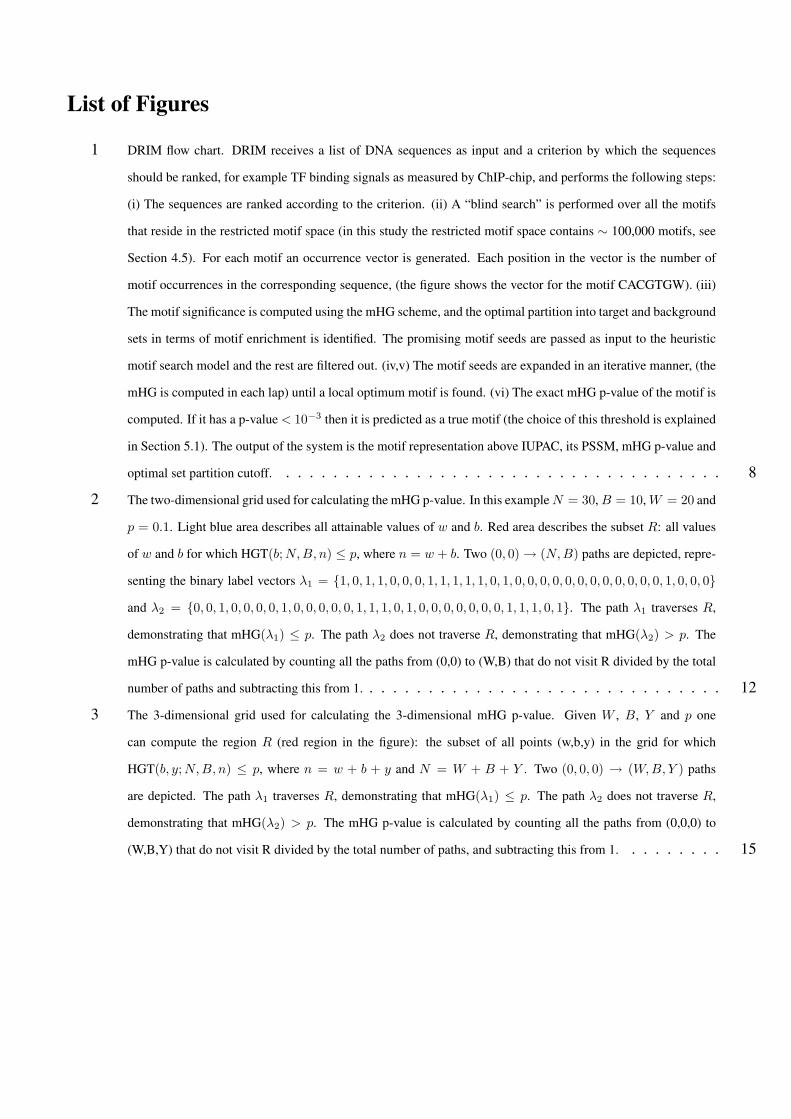
1 DRIM flow chart. DRIM receives a list of DNA sequences as input and a criterion by which the sequences
should be ranked, for example TF binding signals as measured by ChIP-chip, and performs the following steps:
(i) The sequences are ranked according to the criterion. (ii) A “blind search” is performed over all the motifs
that reside in the restricted motif space (in this study the restricted motif space contains ∼ 100,000 motifs, see
Section 4.5). For each motif an occurrence vector is generated. Each position in the vector is the number of
motif occurrences in the corresponding sequence, (the figure shows the vector for the motif CACGTGW). (iii)
The motif significance is computed using the mHG scheme, and the optimal partition into target and background
sets in terms of motif enrichment is identified. The promising motif seeds are passed as input to the heuristic
motif search model and the rest are filtered out. (iv,v) The motif seeds are expanded in an iterative manner, (the
mHG is computed in each lap) until a local optimum motif is found. (vi) The exact mHG p-value of the motif is
computed. If it has a p-value < 10−3 then it is predicted as a true motif (the choice of this threshold is explained
in Section 5.1). The output of the system is the motif representation above IUPAC, its PSSM, mHG p-value and
optimal set partition cutoff. . . . . . . . . . . . . . . . . . . . . . . . . . . . . . . . . . . . . . 8
2 The two-dimensional grid used for calculating the mHG p-value. In this example N = 30, B = 10, W = 20 and
p = 0.1. Light blue area describes all attainable values of w and b. Red area describes the subset R: all values
of w and b for which HGT(b;N,B, n) ≤ p, where n = w + b. Two (0, 0) → (N,B) paths are depicted, repre-
senting the binary label vectors λ1 = 1, 0, 1, 1, 0, 0, 0, 1, 1, 1, 1, 1, 0, 1, 0, 0, 0, 0, 0, 0, 0, 0, 0, 0, 0, 0, 1, 0, 0, 0
and λ2 = 0, 0, 1, 0, 0, 0, 0, 1, 0, 0, 0, 0, 0, 1, 1, 1, 0, 1, 0, 0, 0, 0, 0, 0, 0, 1, 1, 1, 0, 1. The path λ1 traverses R,
demonstrating that mHG(λ1) ≤ p. The path λ2 does not traverse R, demonstrating that mHG(λ2) > p. The
mHG p-value is calculated by counting all the paths from (0,0) to (W,B) that do not visit R divided by the total
number of paths and subtracting this from 1. . . . . . . . . . . . . . . . . . . . . . . . . . . . . . . 12
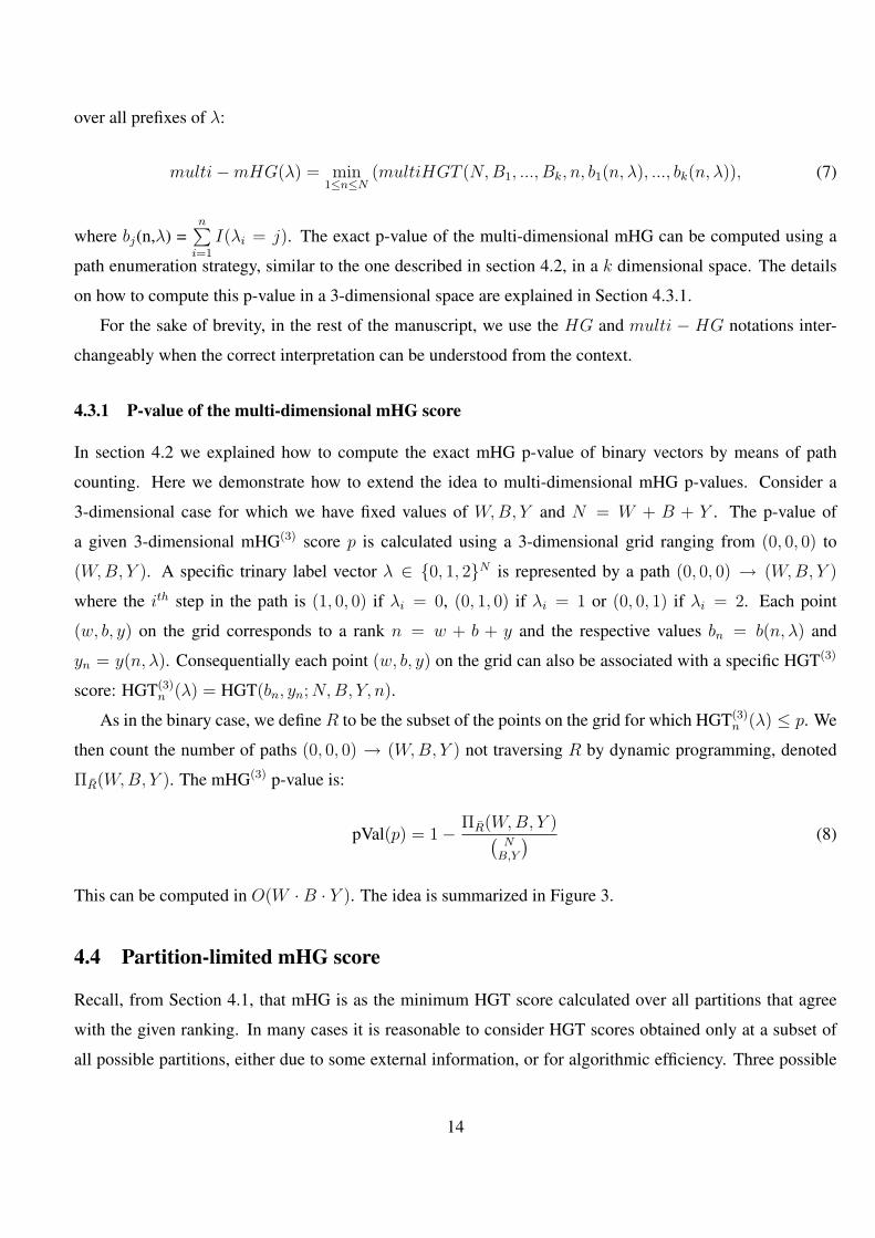
3 The 3-dimensional grid used for calculating the 3-dimensional mHG p-value. Given W , B, Y and p one
can compute the region R (red region in the figure): the subset of all points (w,b,y) in the grid for which
HGT(b, y;N,B, n) ≤ p, where n = w + b + y and N = W + B + Y . Two (0, 0, 0) → (W,B, Y ) paths
are depicted. The path λ1 traverses R, demonstrating that mHG(λ1) ≤ p. The path λ2 does not traverse R,
demonstrating that mHG(λ2) > p. The mHG p-value is calculated by counting all the paths from (0,0,0) to
(W,B,Y) that do not visit R divided by the total number of paths, and subtracting this from 1. . . . . . . . . 15
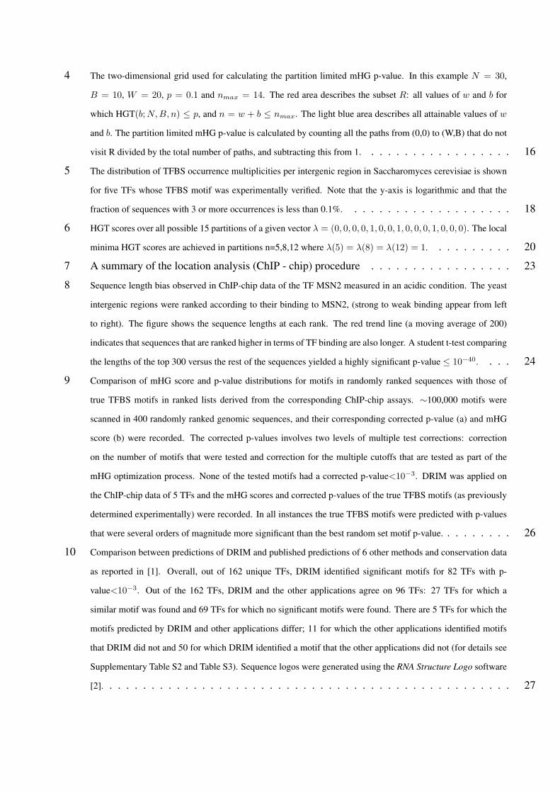
4 The two-dimensional grid used for calculating the partition limited mHG p-value. In this example N = 30,
B = 10, W = 20, p = 0.1 and nmax = 14. The red area describes the subset R: all values of w and b for
which HGT(b;N,B, n) ≤ p, and n = w + b ≤ nmax. The light blue area describes all attainable values of w
and b. The partition limited mHG p-value is calculated by counting all the paths from (0,0) to (W,B) that do not
visit R divided by the total number of paths, and subtracting this from 1. . . . . . . . . . . . . . . . . . 16
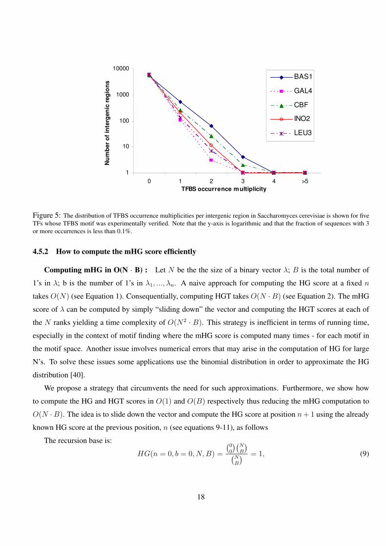
5 The distribution of TFBS occurrence multiplicities per intergenic region in Saccharomyces cerevisiae is shown
for five TFs whose TFBS motif was experimentally verified. Note that the y-axis is logarithmic and that the
fraction of sequences with 3 or more occurrences is less than 0.1%. . . . . . . . . . . . . . . . . . . . 18
6 HGT scores over all possible 15 partitions of a given vector λ = (0, 0, 0, 0, 1, 0, 0, 1, 0, 0, 0, 1, 0, 0, 0). The local
minima HGT scores are achieved in partitions n=5,8,12 where λ(5) = λ(8) = λ(12) = 1. . . . . . . . . . 20
7 A summary of the location analysis (ChIP - chip) procedure . . . . . . . . . . . . . . . . . 23
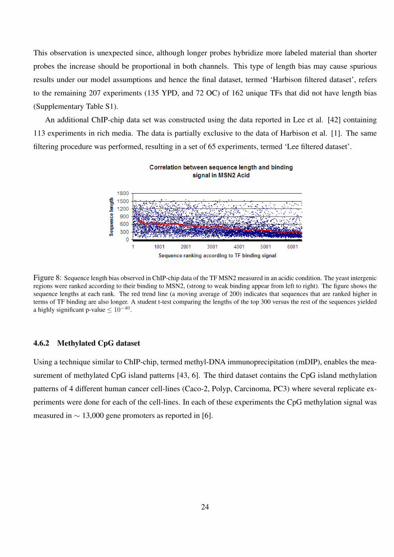
8 Sequence length bias observed in ChIP-chip data of the TF MSN2 measured in an acidic condition. The yeast
intergenic regions were ranked according to their binding to MSN2, (strong to weak binding appear from left
to right). The figure shows the sequence lengths at each rank. The red trend line (a moving average of 200)
indicates that sequences that are ranked higher in terms of TF binding are also longer. A student t-test comparing
the lengths of the top 300 versus the rest of the sequences yielded a highly significant p-value ≤ 10−40. . . . 24
9 Comparison of mHG score and p-value distributions for motifs in randomly ranked sequences with those of
true TFBS motifs in ranked lists derived from the corresponding ChIP-chip assays. ∼100,000 motifs were
scanned in 400 randomly ranked genomic sequences, and their corresponding corrected p-value (a) and mHG
score (b) were recorded. The corrected p-values involves two levels of multiple test corrections: correction
on the number of motifs that were tested and correction for the multiple cutoffs that are tested as part of the
mHG optimization process. None of the tested motifs had a corrected p-value<10−3. DRIM was applied on
the ChIP-chip data of 5 TFs and the mHG scores and corrected p-values of the true TFBS motifs (as previously
determined experimentally) were recorded. In all instances the true TFBS motifs were predicted with p-values
that were several orders of magnitude more significant than the best random set motif p-value. . . . . . . . . 26
10 Comparison between predictions of DRIM and published predictions of 6 other methods and conservation data
as reported in [1]. Overall, out of 162 unique TFs, DRIM identified significant motifs for 82 TFs with p-
value<10−3. Out of the 162 TFs, DRIM and the other applications agree on 96 TFs: 27 TFs for which a
similar motif was found and 69 TFs for which no significant motifs were found. There are 5 TFs for which the
motifs predicted by DRIM and other applications differ; 11 for which the other applications identified motifs
that DRIM did not and 50 for which DRIM identified a motif that the other applications did not (for details see
Supplementary Table S2 and Table S3). Sequence logos were generated using the RNA Structure Logo software
[2]. . . . . . . . . . . . . . . . . . . . . . . . . . . . . . . . . . . . . . . . . . . . . . . . . 27

11 The hypothetical regulatory network of Aro80. Copies of the BSAro80 motif (on the sense and anti sense)
are shown as rectangles on the promoter regions. (a) BSAro80 is conserved in 4 strains of yeast as shown
using the UCSC browser conservation plots. Aro80 regulates the utilization of secondary nitrogen sources
such as aromatic amino acids by binding genes that participate in the catabolism of aromatic amino acids. We
hypothesize that it also binds to its own promoter region and introduces a positive feedback self loop. (b) Part
of the Aro80 promoter sequence is shown with bases of the BSAro80 motif colored in red. Interestingly, there
are three GATA binding sites that are adjacent to the BSAro80 motif (bases colored in green). These sites bind
GATA factors that are known to play a role in nitrogen catabolite repression. We hypothesize that they are also
involved in the repression of Aro80 expression by physically binding to the region near BSAro80 thus making it
inaccessible to Aro80 binding. This in turn breaks the positive feedback loop and represses the expression of
Aro80 itself and other Aro80 regulated genes. . . . . . . . . . . . . . . . . . . . . . . . . . . . . . 30
12 Compatibility between the BSAro80 motif identified by DRIM and previously reported mutagenesis studies [3].
The Aro9 promoter region from base -169 to -133 as well as 6 other copies containing mutations and deletions
are shown. These regions were used in order to construct hybrid promoters and measure the expression of a
reporter gene, which is dependent on the binding of Aro80 to the promoter[3]. The two partially overlapping
copies of BSAro80 that reside in the Aro9 promoter and an additional sequence element that is similar to the
canonic BSAro80 (2 different bases) are marked with green and blue arrows respectively. It can be seen that
the expression values can be explained in terms of intact BSAro80 copies, i.e more intact copies yield higher
expression. . . . . . . . . . . . . . . . . . . . . . . . . . . . . . . . . . . . . . . . . . . . . 31
13 Visualization of CA repeat occurrences in the yeast genome and their correlation with TF binding. ∼6000
intergenic regions were ranked according to their binding to the TF AFT2 in a H2O2Hi ChIP-chip experiment
[1] and the motif CACACACA was searched in each of the regions. On the left is the motif occurrence vector
with white, black, blue and red lines indicating whether the corresponding region contains 0, 1, 2 or >2 motif
occurrences respectively. It can be seen that the top of the vector is significantly more dense than the rest of
the vector indicating that the CA repeats are highly correlated with AFT2 binding. In the center is the motif
occurrence map in which the blue lines mark the bases of the motif occurrences. It can be seen that that the
density of motif occurrences increases in regions that are ranked high in the list . On the right is a plot of the
expected vs. observed cumulative motif occurrences. The x-axis represents the ranked intergenic regions and
the y-axis is the cumulative motif occurrence as function of rank. The height of the y-axis is the total number of
motif occurrences. . . . . . . . . . . . . . . . . . . . . . . . . . . . . . . . . . . . . . . . . . 32

14 (a) Schematic representation of Met4-Met28-CBF and Met4-Met28-Met31/32 complexes [4, 5]. (b) A hypo-
thetical Met4-Met28-CBF-Met31/32 complex. Immuno-precipitation of any of the TFs in the complex will
precipitate the same set of sequences, which explains why DRIM identifies the same two motifs for all TFs in
the complex. . . . . . . . . . . . . . . . . . . . . . . . . . . . . . . . . . . . . . . . . . . . . 33
15 Occurrences of CA repeats in the human genome and their correlation to CpG methylation. (a) ∼13,000 pro-
moters were ranked according to their CpG methylation in a human carcinoma cell-line [6]. Similarly to Figure
13 from left to right are the occurrence vector, motif occurrence map and the plot of the cumulative motif oc-
currence, all generated for the motif CACACACA. It can be seen that the CA repeats are highly correlated with
CpG methylation as indicated by the increased density of the motif occurrences at the regions that are ranked
top. (b) A control experiment in which the promoters are randomly ranked. It can be seen that the CA repeat
occurrences are distributed uniformly and the observed cumulative motif occurrence is close to the expected. . 36
16 Comparison between HG and mHG enrichment. The mHG and HG methods were applied to ChIP-chip data
of 6 TFs. The sequences were ranked according to the ChIP-chip binding signal and the enrichment of the
correct binding motif was recorded using mHG and HG with fixed target sets containing the top 10, 100, 1000
sequences as well as all sequences with ChIP-chip signal < 10−3. All scores were corrected for multiple motif
testing. The mHG score is also corrected for the multiple cutoff testing. The 10−3 and mHG cutoffs for each
experiment are shown. It can be seen that the two cutoffs are significantly different and that for all the tested
TFs mHG produces better results than HG in terms of enrichment of the true motif. . . . . . . . . . . . . 38
17 Comparison of the target sets sizes as determined by the fixed versus the mHG flexible cutoffs. Each dot
represents a ChIP-chip experiment where the x and y coordinates are the number of promoters with p < 10−3
(standard cutoff) and the number of promoters as determined by the mHG cutoff, respectively. The dotted line
is x = y. TF names are given in Table S4 . . . . . . . . . . . . . . . . . . . . . . . . . . . . . . . 39
18 Motif occurrences in the top 59 (of ∼6000) promoters that were ranked according to Met32 binding signal. A
comparison is made between the data driven mHG cutoff and the arbitrary fixed cutoff. It can be seen that the
motifs are significantly more enriched when the list is partitioned using the mHG cutoff. . . . . . . . . . . 40
S1 Comparison of p-value bounds, exact p-value calculation and observed frequencies of mHG scores for two
synthetic cases: a) N = 600, B = 300, b) N = 330, B = 30. In each case the following values were generated
for several different mHG scores: lower bound (p), trivial upper bound (Np), tighter upper bound(Bp), exact
p-value calculation (pVal) and observed p-values over 10,000 random instances (sim). Note the improvement
of the tighter upper bound (Bp) when N >> B. . . . . . . . . . . . . . . . . . . . . . . . . . . . . 49
S2 Comparison of the mHG and HG methods on simulations of motif occurrence vectors. The vectors were
generated according to a rank dependent distribution (Section 7.3) with 18 different parameter combinations
(a = 10, 50, 100; b = 0.01, 0.05, 0.1;u = 0.01, 0.1). The -log fraction between mHG and HG p-values in cases
where the p-value of one of the methods was smaller than 10−3 are shown. . . . . . . . . . . . . . . . . 51
S3 An example of the output of GOviz. A set of genes were ranked according to differential expression of 31
patients with CVD (cardio-vascular disease, either ischemic or non-ischemic) versus 6 patients with none failure
hearts as reported in [7]. The enriched GO terms (mHG p-value < 10−2 after bonfferoni correction for multiple
GO term testing) and their parent GO terms up to the root are shown. The colors reflect the level of enrichment
(yellow: 10−2 to 10−4, orange: 10−4 to 10−6, red: 10−6 to 10−8 ) . . . . . . . . . . . . . . . . . . . . 53
S4 Observed versus expected length bias. For each of the 148 OC ChIP-chip experiments reported in [1] we ranked
the yeast intergenic sequences according to their binding signal. The lengths of the top 300 sequences in each
experiment were compared to the lengths of the rest of the sequences using a student t-test. The x axis is the
t-test p-value and y(x) is the number of TF experiments with p ≤ x. The blue line is the observed cumulative
distribution of the t-test p-values in the 148 experiments. The red line is the expected cumulative distribution
of t-test p-values in randomly permuted sequence rankings. It can be seen that over half of the ChIP-chip
experiments have a statistically significant difference between the lengths of sequences that bind the TF the
strongest compared to the lengths of the rest of the sequences. . . . . . . . . . . . . . . . . . . . . . . 54
List of Tables
1 Examples of TFs for which DRIM identifies novel motifs.We further investigated these motifs and show evi-
dence that indicate they are biologically functional. YPD, H2O2 and SM denote the ChIP-chip experimental
conditions [1] in which the motifs were identified. . . . . . . . . . . . . . . . . . . . . . . . . . . . 28
2 Enriched motifs associated with CpG methylation in 4 human cancer cell-lines and comparison to motifs in
regions bound by the Polycomb complex. ‘# of experiments’ corresponds to the number of replicate experiments
of the same cell-line in which the same motif was independently identified. The CA repeat motifs have a variable
length. ’Polycomb complex motif’ denotes motifs that appear in regions bound by the Polycomb complex
[8, 9, 10]. The motifs that are marked with a ‘∗’ have G-C content > 66%. Their enrichments are partially
attributed to the G-C content bias that is found in the CpG methylation data. . . . . . . . . . . . . . . . 35

1 Abstract
Computational methods for discovery of sequence elements that are enriched in a target set compared to a
background set are fundamental in molecular biology research. One example is the discovery of transcription
factor binding motifs that are inferred from ChIP-chip (Chromatin Immuno-Precipitation on a microarray)
measurements. Several major challenges in sequence motif discovery still require consideration: (i) the need
for a principled approach to partitioning the data into target and background sets; (ii) the lack of rigorous
models and of an exact p-value for measuring motif enrichment; (iii) the need for an appropriate framework
for accounting for motif multiplicity; (iv) the tendency, in many of the existing methods, to report presumably
significant motifs even when applied to randomly generated data. In this study we present a statistical frame-
work for discovering enriched sequence elements in ranked lists that resolves the above four issues. Based on
this framework we developed a software application, termed DRIM (Discovery of Rank Imbalanced Motifs),
which identifies sequence motifs in lists of ranked DNA sequences.
We applied DRIM to ChIP-chip and CpG methylation data and obtained the following results: (i) Iden-
tification of 50 novel putative transcription factor (TF) binding sites in yeast ChIP-chip data. The biological
function of some of them was further investigated and used in order to gain new insights on transcription
regulation networks in yeast. For example, our discoveries enable the elucidation of the network of the TF
ARO80.Another finding concerns a systematic TF binding enhancement to sequences containing CA repeats
that suggests these repetitive elements play a mechanistic role in TF binding. (ii) Discovery of novel motifs
in human cancer CpG methylation data. Remarkably, most of these motifs are similar to DNA sequence
elements bound by the Polycomb complex that promotes histone methylation. Our findings thus support a
model in which histone methylation and CpG methylation are mechanistically linked.
Overall, we demonstrate that our statistical framework embodied in the DRIM software tool is highly
effective for identifying regulatory sequence elements in a variety of applications ranging from expression
and ChIP-chip to CpG methylation data. DRIM is publicly available at: http://bioinfo.cs.technion.ac.il/drim.
1
2 Abbreviations
• TF, transcription factor;
• TFBS, transcription factor binding site;
• ChIP-chip, Chromatin Immuno-precipitation chip;
• mDIP, methyl-DNA immunoprecipitation;
• DRIM, discovery of rank imbalanced motifs;
• HG, Hyper-geometric;
• HGT, Hyper-geometric tail;
• mHG, minimal hyper-geometric;
• MM, Markov model.
• MOV, motif occurrence vector
• GO, gene ontology
2
3 Introduction
3.1 Background
This study examines the problem of discovering “interesting” sequence motifs in biological sequence data.
A widely accepted and more formal definition of this task is:
Given a target set and a background set of sequences (or a background model), identify sequence motifs
that are enriched in the target set compared to the background set.
The purpose of this study is to extend this formulation and make it more flexible so as to enable the determi-
nation of the target and background set in a data driven manner.
Discovery of sequences motifs or other attributes that are enriched in a target set compared to a back-
ground set (or model) has become increasingly useful in a wide range of applications in molecular biology
research. For example, discovery of DNA sequence motifs that are over-abundant in a set of promoter re-
gions of co-expressed genes (determined by clustering of expression data) can suggest an explanation for this
co-expression. Another example is the discovery of DNA sequences that are enriched in a set of promoter re-
gions to which a certain transcription factor (TF) binds strongly, inferred from ChIP-chip [11] measurements.
Such enriched sequence motifs are promising TF binding sites (TFBS) candidates. The same principle may
be extended to many other applications such as discovery of genomic elements enriched in a set of highly
methylated CpG island sequences [6].
Due to its importance, this task of discovering enriched DNA subsequences and capturing their corre-
sponding motif profile has gained much attention in the literature. Any approach to motif discovery must
address several fundamental issues: defining a motif representation, choosing a background model, devising
a score for capturing motif enrichment and devising a scheme for probing the motif space. We discuss these
issues in the following subsections (Section 3.1.1 - 3.1.4).
3.1.1 Motif representations
The first key issue in motif discovery is to define “What exactly is a biological sequence motif?” and devise
an appropriate computer model to capture it. Of course, different biological phenomena give rise to different
types of motifs and may require different types of models. For example, TFBS motifs differ from splicing
signal motifs in aspects such as motif length, variability, multiplicity and position in the genome.
There are several strategies for motif representation. The first uses a k-mer of symbols above A,C,G,Tto represent a motif. However, this model is over-simplistic and does not capture the stochasticity that often
appears in real biological sequence motifs. An enhancement of this model is a k-mer above the 15 symbol
3
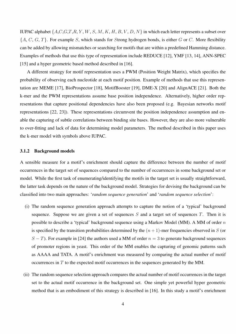
IUPAC alphabet A,C,G,T ,R, Y , W , S, M , K, H , B, V , D, N in which each letter represents a subset over
A, C, G, T. For example S, which stands for Strong hydrogen bonds, is either G or C. More flexibility
can be added by allowing mismatches or searching for motifs that are within a predefined Hamming distance.
Examples of methods that use this type of representation include REDUCE [12], YMF [13, 14], ANN-SPEC
[15] and a hyper geometric based method described in [16].
A different strategy for motif representation uses a PWM (Position Weight Matrix), which specifies the
probability of observing each nucleotide at each motif position. Example of methods that use this represen-
tation are MEME [17], BioProspector [18], MotifBooster [19], DME-X [20] and AlignACE [21]. Both the
k-mer and the PWM representations assume base position independence. Alternatively, higher order rep-
resentations that capture positional dependencies have also been proposed (e.g. Bayesian networks motif
representations [22, 23]). These representations circumvent the position independence assumption and en-
able the capturing of subtle correlations between binding site bases. However, they are also more vulnerable
to over-fitting and lack of data for determining model parameters. The method described in this paper uses
the k-mer model with symbols above IUPAC.
3.1.2 Background models
A sensible measure for a motif’s enrichment should capture the difference between the number of motif
occurrences in the target set of sequences compared to the number of occurrences in some background set or
model. While the first task of enumerating/identifying the motifs in the target set is usually straightforward,
the latter task depends on the nature of the background model. Strategies for devising the background can be
classified into two main approaches: ‘random sequence generation’ and ‘random sequence selection’:
(i) The random sequence generation approach attempts to capture the notion of a ‘typical’ background
sequence. Suppose we are given a set of sequences S and a target set of sequences T . Then it is
possible to describe a ‘typical’ background sequence using a Markov Model (MM). A MM of order n
is specified by the transition probabilities determined by the (n + 1)-mer frequencies observed in S (or
S − T ). For example in [24] the authors used a MM of order n = 3 to generate background sequences
of promoter regions in yeast. This order of the MM enables the capturing of genomic patterns such
as AAAA and TATA. A motif’s enrichment was measured by comparing the actual number of motif
occurrences in T to the expected motif occurrences in the sequences generated by the MM.
(ii) The random sequence selection approach compares the actual number of motif occurrences in the target
set to the actual motif occurrence in the background set. One simple yet powerful hyper geometric
method that is an embodiment of this strategy is described in [16]. In this study a motif’s enrichment
4
was captured by computing the probability of the observed number of motif occurrences in T under the
null hypothesis that the sequences in T were drawn from S at random.
One major advantage of the random sequence selection over the random sequence generation approach is
that the first does not make any assumptions on the distribution of nucleotides. Such assumptions often
fail to capture inherent complexities in genomic sequences and in turn lead to false motif predictions. For
example, genomic patterns such as repetitive elements (e.g., CA or poly-A repeats) may be as long as 60
bases. However, constructing MMs of sufficient order to capture these events is unfeasible.
The framework described in our study uses the random sequence selection approach and is a natural
extension of the approach of [16].
3.1.3 Motif enrichment scores
We turn to examine the question of how to devise a scoring scheme that captures motif enrichment. Many
strategies for scoring motifs have been suggested in the literature. YMF [13, 14] and the work described
in [24] associate each motif with a z-score that measures the number of standard divinations by which the
total number of observed motifs in the target set exceed the expected number of motifs in a background set
of sequences generated by a MM. The hyper-geometric approach of [16] uses the hyper-geometric tail as a
measure for mtif enrichment. AlignACE [21] uses a Gibbs sampling algorithm for finding global sequence
alignments and produces a MAP score. This score is an internal metric used to determine the significance
of an alignment. MEME [17] uses an expectation maximization strategy and outputs the log-likelihood and
relative entropy associated with each motif.
It is important to note that other then the work of [16], which produces an enrichment p-value, the other
studies mentioned above produce a score that does not lend itself to such straight forward statistical interpre-
tation. Instead, they use thresholds on their enrichment scores to determine what constitutes a significantly
enriched motif or alternatively result to Monte-Carlo simulations on these scores to produce simulation based
p-values.
3.1.4 Scanning the motif space
Once a motif score is devised most methods scan through a predefined motif space in search of significantly
enriched motifs. Defining “What is the appropriate motif space?” is thus a fundamental issue. In some cases,
the size of all biologically viable motifs can be restricted and the corresponding motif space size is amenable
to exhaustive search. An example of such a case is described in [14] where TFBS motifs in the yeast genome,
many of which have been shown to have a characteristics length of 6-10, are searched. However, other
5
instances such as TFBS of mammalians that have larger and fuzzier motifs lead to a practically infinite size
of motif space (e.g. all 1520 motifs that reside in the space of 20-mers above the 15 symbol IUPAC alphabet),
which cannot be scanned exhaustively in terms of running time. To deal with this some approaches use a
heuristic search strategy (e.g., [17]). Other approaches scan part of the motif space exhaustively and generate
motif seeds that are then further enlarged in a heuristic manner (e.g., [16]). Their underlying assumption is
that large motifs are built from shorter motifs seeds that are sufficiently enriched to be detected. The study
described herein makes this assumption as well.
Several excellent reviews narrate the different strategies for motif detection and use quantitative bench-
marking to compare their performance [25, 26, 27, 28, 29]. A related aspect of motif discovery, which is
outside the scope of this study, focuses on properties of clusters and modules of TF binding sites (TFBS).
Examples of approaches that search for combinatorial patterns and modules underlying TF binding and gene
expression include [30, 31, 32, 33, 34].
3.2 Open challenges in motif discovery
One issue of motif discovery that is often overlooked, concerns the partition of the input set of sequences
into target and background sets. Many methods rely on the user to provide these two sets and search for
motifs that are overabundant in the former set compared to the latter. However, the question of how to
partition the data, i.e. set the boundary between the sets, is often unclear and the exact choice of sequences
in each set arbitrary. For example, suppose that one wishes to identify motifs within promoter sequences
that constitute putative TFBS. An obvious strategy would be to partition the set of promoter sequences into
target and background sets according to the TF binding signal (as measured by ChIP-chip experiments). The
two sets would contain the sequences to which the TF binds “strongly” and “weakly” respectively. A motif
detection algorithm could then be applied to find motifs that are over-abundant in the target set compared
to the background set. In this scenario the positioning of the cutoff between the strong and weak binding
signal is somewhat arbitrary. Obviously, the final outcome of the motif identification process can be highly
dependent on this choice of cutoff. A stringent cutoff will result in the exclusion of informative sequences
from the target set while a promiscuous cutoff will cause inclusion of non-relevant sequences - both extremes
hinder the accuracy of motif prediction. This example demonstrates a fundamental difficulty in partitioning
most types of data. Several methods attempt to circumvent this hurdle. For example, REDUCE [12] uses a
regression model on the entire set of sequences. However it is difficult to justify this model in the context
of multiple motif occurrence (as explained below). In other work a variant of the Kolmogorov-Smirnov test
was used for motif discovery [35]. This approach successfully circumvents arbitrary data partition. However
it has other limitations such as the failure to address multiple motif occurrences in a single promoter, and
6

the lack of an exact characterization of the null distribution. Overall, the following four major challenges in
motif discovery still require consideration:
(c1) The cutoff used in order to partition data into a target set and background set of sequences is often
chosen arbitrarily.
(c2) Lack of an exact statistical score and p-value for motif enrichment. Current methods typically use
arbitrarily-set thresholds or simulations, which are inherently limited in precision and costly in terms
of running time.
(c3) A need for an appropriate framework that accounts for multiple motif occurrences in a single promoter.
For example, how should one quantify the significance of a single motif occurrence in a promoter
against two motif occurrences in a promoter? Linear models [12] assume that the weight of the latter
is double that of the former. However, it is difficult to justify this approach since biological systems
do not necessarily operate in such a linear fashion. Another issue related to motif multiplicity is low
complexity or repetitive regions. These regions often contain multiple copies of degenerate motifs
(e.g. ploy A repeats). Since the nucleotide frequency underlying these regions substantially deviates
from the standard background frequency they often cause false motif discoveries. Consequently, most
methods mask these regions in the preprocessing stage and thereby loose vital information that might
reside therein.
(c4) Criticism has been made over the fact that motif discovery methods tend to report presumably signif-
icant motifs even when applied on randomly generated data [1]. These motifs are clear cases of false
positives and should be avoided.
3.3 Data lends itself to ranking in a natural manner
In this paper we describe a novel method that attempts to solve the above mentioned four challenges in a
principled manner. It exploits the following observation: Data often lends itself to ranking in a natural manner,
e.g. ranking sequences according to TF binding signal; ranking according to CpG methylation signal; ranking
according to distance in expression space from a set of co-expressed genes; ranking according to differential
expression; etc. We exploit this inherent ranking property of biological data in order to circumvent the need
for an arbitrary and difficult to justify data partition. Consequently, we propose the following formulation of
the motif finding task:
Given a list of ranked sequences, identify motifs that are over-abundant at either end of the list.
7
Input
10-8
GCACGTGATA…
10-6
AGCGCGG...
10-5
GGGAGCACGTGAA...
10-3
GAACACGTGTGTG…
10-2
ACACGTGGGAAA…
10-2
ACGTAAAAATA
10-1
ACACGTTTAAAA
.
.
.
10-1
GGGAGAGGGGA
(i)
Sequence
ranking
(ii)
Occurrence
vector generator
(iii)
Computing mHG
enrichment
10-1
GGGAGAGGGGA
10-8
GCACGTGATA…
10-5
GGGAGCACGTGAA...
10-2
ACACGTGGGAAA…
10-2
ACGTAAAAATA
10-1
ACACGTTTAAAA
10-3
GAACACGTGTGTG…
.
.
.
10-6
AGCGCGG...
GCACGTGATA…
AGCGCGG...
GGGAGCACGTGAA...
GAACACGTGTGTG…
ACACGTGTGAAA…
ACGTAAAAATA
ACACGTTTAAAA
.
.
.
GGGAGAGGGGA
1
0
1
1
1
0
0
.
.
.
0
Weak binding
Strong binding
Optimal partition
cutoff
background
set
target set
Motif space sampler Motif
filtering
(iv)
Motif
expander
(v)
Computing mHG
enrichment
(vi)
Computing
exact p-value
Motif
similarity
filtering Motif seeds
CACGTGW
CGGNNNNNNCCG
Weak bindingStrong binding
outputP-value=10
-7
Exhaustive search of restricted motif space
Heuristic search of entire motif space
DRIM flow chart
CACGTGW
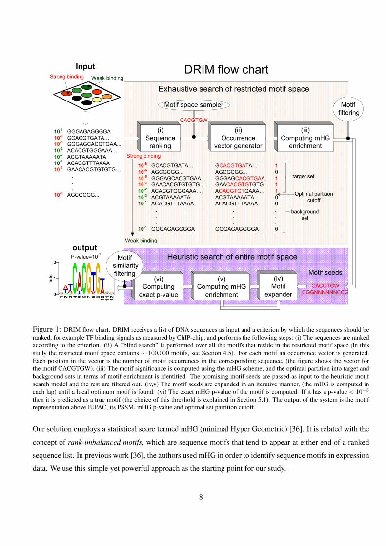
Figure 1: DRIM flow chart. DRIM receives a list of DNA sequences as input and a criterion by which the sequences should beranked, for example TF binding signals as measured by ChIP-chip, and performs the following steps: (i) The sequences are rankedaccording to the criterion. (ii) A “blind search” is performed over all the motifs that reside in the restricted motif space (in thisstudy the restricted motif space contains ∼ 100,000 motifs, see Section 4.5). For each motif an occurrence vector is generated.Each position in the vector is the number of motif occurrences in the corresponding sequence, (the figure shows the vector forthe motif CACGTGW). (iii) The motif significance is computed using the mHG scheme, and the optimal partition into target andbackground sets in terms of motif enrichment is identified. The promising motif seeds are passed as input to the heuristic motifsearch model and the rest are filtered out. (iv,v) The motif seeds are expanded in an iterative manner, (the mHG is computed ineach lap) until a local optimum motif is found. (vi) The exact mHG p-value of the motif is computed. If it has a p-value < 10−3
then it is predicted as a true motif (the choice of this threshold is explained in Section 5.1). The output of the system is the motifrepresentation above IUPAC, its PSSM, mHG p-value and optimal set partition cutoff.
Our solution employs a statistical score termed mHG (minimal Hyper Geometric) [36]. It is related with the
concept of rank-imbalanced motifs, which are sequence motifs that tend to appear at either end of a ranked
sequence list. In previous work [36], the authors used mHG in order to identify sequence motifs in expression
data. We use this simple yet powerful approach as the starting point for our study.
8

3.4 Overview
The rest of this manuscript is divided into two main parts: in the Methods (Section 4) we develop the mHG
probabilistic and algorithmic framework and explain how we deal with challenges (c1)-(c3) introduced in
Section 3.2. In the Results (Section 5) we address challenge (c4) and describe novel biological findings that
were obtained by applying our algorithms to biological data. Each part is self contained and can be read
separately.
9

4 Materials and Methods
4.1 The minimum hyper-geometric (mHG) score
In this subsection we introduce the basics of the mHG statistics, and demonstrate how it can be applied in a
straight forward manner to eliminate the need for an arbitrary choice of threshold. To explain the biological
motivation of mHG consider the following scenario: suppose we have a set of promoter regions each asso-
ciated with a measurement, e.g. a TF binding signal as measured by ChIP-chip [11]. We wish to determine
whether a particular motif specified in IUPAC notation, say CASGTGW, is likely to be a TFBS motif. We
rank the promoters according to their binding signals - strong binding at top of the list and the weak at the
bottom (Figure 1i). Next, we generate a binary occurrence vector with 1 or 0 entries dependent on whether or
not the respective promoter contains a copy of the motif (Figure 1ii). For simplicity we ignore cases where
a promoter contains multiple copies of the motif, a restriction that will later be removed. Motifs that yield
binary vectors with a high density of 1’s at the top of the list are good candidates for being TFBS.
Let us assume for the moment that we know where to put a cutoff on the TF binding signal. The data could
then be separated into ‘strong binding promoters’ (i.e. the target set) and ‘weak binding promoters’ (i.e. the
background set). We are now interested in a particular motifs for which the target set contains significantly
more occurrences than the background set. Let N be the total number of promoters, B of which contain the
motif, and n the size of the target set. Let X be a random variable describing the number of motif occurrences
in the target set. Assuming a uniform distribution over all occurrence vectors with these characteristics, X
has a Hyper-Geometric (HG) distribution. Namely, the probability of finding exactly b occurrences in the
target set is:
Prob(X = b) = HG(b; N, B, n) =
(nb
)(N−nB−b
)(NB
) . (1)
The tail probability of finding b or more occurrences in the target set is:
Prob(X ≥ b) = HGT(b; N, B, n) =
min(n,B)∑i=b
(ni
)(N−nB−i
)(NB
) . (2)
As we don’t really know the target set and therefore do not know n nor b we employ a strategy that seeks
a partition for which the motif enrichment is the most significant, and compute the enrichment under that
particular partition. Formally, consider a set of ranked elements and some binary labeling of the set λ =
λ1, ..., λN ∈ 0, 1N . The binary labels represent the attribute (e.g. motif occurrence). The minimum Hyper-
10
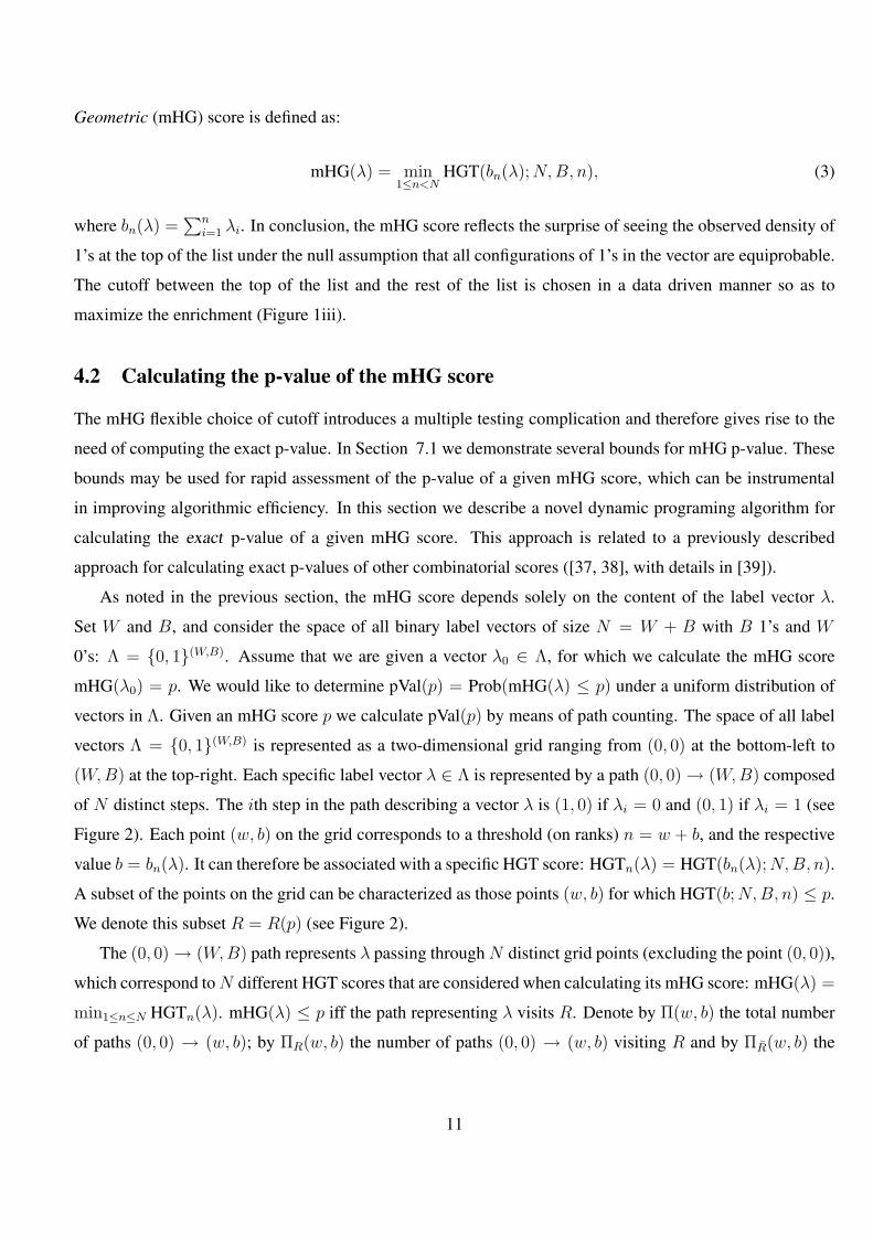
Geometric (mHG) score is defined as:
mHG(λ) = min1≤n<N
HGT(bn(λ); N, B, n), (3)
where bn(λ) =∑n
i=1 λi. In conclusion, the mHG score reflects the surprise of seeing the observed density of
1’s at the top of the list under the null assumption that all configurations of 1’s in the vector are equiprobable.
The cutoff between the top of the list and the rest of the list is chosen in a data driven manner so as to
maximize the enrichment (Figure 1iii).
4.2 Calculating the p-value of the mHG score
The mHG flexible choice of cutoff introduces a multiple testing complication and therefore gives rise to the
need of computing the exact p-value. In Section 7.1 we demonstrate several bounds for mHG p-value. These
bounds may be used for rapid assessment of the p-value of a given mHG score, which can be instrumental
in improving algorithmic efficiency. In this section we describe a novel dynamic programing algorithm for
calculating the exact p-value of a given mHG score. This approach is related to a previously described
approach for calculating exact p-values of other combinatorial scores ([37, 38], with details in [39]).
As noted in the previous section, the mHG score depends solely on the content of the label vector λ.
Set W and B, and consider the space of all binary label vectors of size N = W + B with B 1’s and W
0’s: Λ = 0, 1(W,B). Assume that we are given a vector λ0 ∈ Λ, for which we calculate the mHG score
mHG(λ0) = p. We would like to determine pVal(p) = Prob(mHG(λ) ≤ p) under a uniform distribution of
vectors in Λ. Given an mHG score p we calculate pVal(p) by means of path counting. The space of all label
vectors Λ = 0, 1(W,B) is represented as a two-dimensional grid ranging from (0, 0) at the bottom-left to
(W, B) at the top-right. Each specific label vector λ ∈ Λ is represented by a path (0, 0) → (W, B) composed
of N distinct steps. The ith step in the path describing a vector λ is (1, 0) if λi = 0 and (0, 1) if λi = 1 (see
Figure 2). Each point (w, b) on the grid corresponds to a threshold (on ranks) n = w + b, and the respective
value b = bn(λ). It can therefore be associated with a specific HGT score: HGTn(λ) = HGT(bn(λ); N, B, n).
A subset of the points on the grid can be characterized as those points (w, b) for which HGT(b; N, B, n) ≤ p.
We denote this subset R = R(p) (see Figure 2).
The (0, 0) → (W, B) path represents λ passing through N distinct grid points (excluding the point (0, 0)),
which correspond to N different HGT scores that are considered when calculating its mHG score: mHG(λ) =
min1≤n≤N HGTn(λ). mHG(λ) ≤ p iff the path representing λ visits R. Denote by Π(w, b) the total number
of paths (0, 0) → (w, b); by ΠR(w, b) the number of paths (0, 0) → (w, b) visiting R and by ΠR(w, b) the
11

Figure 2: The two-dimensional grid used for calculating the mHG p-value. In this example N = 30, B = 10,W = 20 and p = 0.1. Light blue area describes all attainable values of w and b. Red area describes the subsetR: all values of w and b for which HGT(b;N,B, n) ≤ p, where n = w + b. Two (0, 0) → (N,B) paths are de-picted, representing the binary label vectors λ1 = 1, 0, 1, 1, 0, 0, 0, 1, 1, 1, 1, 1, 0, 1, 0, 0, 0, 0, 0, 0, 0, 0, 0, 0, 0, 0, 1, 0, 0, 0 andλ2 = 0, 0, 1, 0, 0, 0, 0, 1, 0, 0, 0, 0, 0, 1, 1, 1, 0, 1, 0, 0, 0, 0, 0, 0, 0, 1, 1, 1, 0, 1. The path λ1 traverses R, demonstrating thatmHG(λ1) ≤ p. The path λ2 does not traverse R, demonstrating that mHG(λ2) > p. The mHG p-value is calculated by countingall the paths from (0,0) to (W,B) that do not visit R divided by the total number of paths and subtracting this from 1.
number of paths (0, 0) → (w, b) not visiting R. We then have:
pVal(p) =|λ ∈ Λ : mHG(λ) ≤ p|
|Λ|=
ΠR(W, B)
Π(W, B)=
Π(W, B)− ΠR(W, B)
Π(W, B)= 1− ΠR(W, B)
Π(W, B)(4)
We calculate ΠR(w, b) by means of dynamic programming. Initially, set ΠR(0, 0) = 1, ΠR(−1, b) = 0 for
0 ≤ b ≤ B and ΠR(w,−1) = 0 for 0 ≤ w ≤ W . Then, for each 0 ≤ w ≤ W , and 0 ≤ b ≤ B calculate
ΠR(w, b) using the formula:
• 0, if (w, b) ∈ R
• ΠR(w, b) = ΠR(w − 1, b) + ΠR(w, b− 1), if (w, b) /∈ R
In summary, to compute the p-value pVal(p) of an mHG score p we first calculate ΠR(W, B). Trivially,
we have Π(W, B) =(
W+BB
)and pVal(p) may be directly computed from (4). The time complexity of the
algorithm is O(W ·B), which is also O(N2) obviously.
4.3 Multi-dimensional mHG Score
So far we have dealt with enrichment of binary attributes, in which a 1 or 0 indicated whether or not the
attribute appeared. There are cases where one would like to associate a number with an attribute. We revisit
our example from section 4.1 in which we tried to determine whether a particular motif is likely to be a
TFBS motif. The promoters were ranked according to their binding signals and the corresponding binary
12
occurrence vector was generated. Notice, that some promoters may contain several copies of a particular
motif. Clearly, this information is valuable, as it may affect TF binding potential, and should be incorporated
in the enrichment analysis. However, how exactly to incorporate this information is not obvious. For example,
consider two motif occurrence vectors generated for two different motifs. The top 10 entries of the vectors
are all 1’s and 2’s respectively. Is the second motif more enriched than the first? Obviously, this depends on
how rare 2 motif occurrences are compared to 1 in the corresponding vectors. If the frequency of 2’s is lower
than that of 1’s then the second motif is more significant. However, if they are equally frequent (this is often
the case for degenerate motifs such as poly A’s) then both motifs are equally enriched.
To quantitatively capture this notion and address motif multiplicity in a data driven manner, we propose a
multi-dimensional hyper geometric model, which extends the previously-defined framework for enrichment
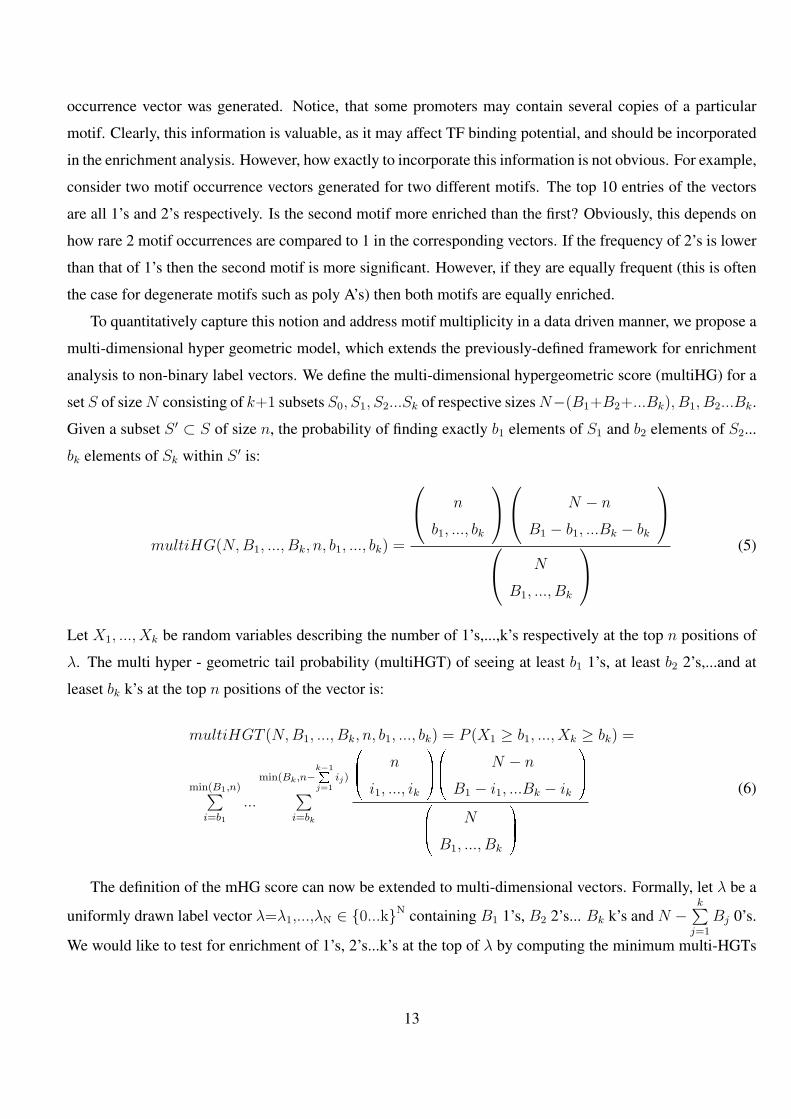
analysis to non-binary label vectors. We define the multi-dimensional hypergeometric score (multiHG) for a
set S of size N consisting of k+1 subsets S0, S1, S2...Sk of respective sizes N−(B1+B2+...Bk), B1, B2...Bk.
Given a subset S ′ ⊂ S of size n, the probability of finding exactly b1 elements of S1 and b2 elements of S2...
bk elements of Sk within S ′ is:
multiHG(N, B1, ..., Bk, n, b1, ..., bk) =
n
b1, ..., bk
N − n
B1 − b1, ...Bk − bk
N
B1, ..., Bk
(5)
Let X1, ..., Xk be random variables describing the number of 1’s,...,k’s respectively at the top n positions of
λ. The multi hyper - geometric tail probability (multiHGT) of seeing at least b1 1’s, at least b2 2’s,...and at
leaset bk k’s at the top n positions of the vector is:
multiHGT (N, B1, ..., Bk, n, b1, ..., bk) = P (X1 ≥ b1, ..., Xk ≥ bk) =
min(B1,n)∑i=b1
...
min(Bk,n−k−1Pj=1
ij)∑i=bk
0BB@
n
i1, ..., ik
1CCA
0BB@
N − n
B1 − i1, ...Bk − ik
1CCA
0BB@
N
B1, ..., Bk
1CCA
(6)
The definition of the mHG score can now be extended to multi-dimensional vectors. Formally, let λ be a
uniformly drawn label vector λ=λ1,...,λN ∈ 0...kN containing B1 1’s, B2 2’s... Bk k’s and N −k∑
j=1
Bj 0’s.
We would like to test for enrichment of 1’s, 2’s...k’s at the top of λ by computing the minimum multi-HGTs
13
over all prefixes of λ:
multi−mHG(λ) = min1≤n≤N
(multiHGT (N, B1, ..., Bk, n, b1(n, λ), ..., bk(n, λ)), (7)
where bj(n,λ) =n∑
i=1
I(λi = j). The exact p-value of the multi-dimensional mHG can be computed using a
path enumeration strategy, similar to the one described in section 4.2, in a k dimensional space. The details
on how to compute this p-value in a 3-dimensional space are explained in Section 4.3.1.
For the sake of brevity, in the rest of the manuscript, we use the HG and multi − HG notations inter-
changeably when the correct interpretation can be understood from the context.
4.3.1 P-value of the multi-dimensional mHG score
In section 4.2 we explained how to compute the exact mHG p-value of binary vectors by means of path
counting. Here we demonstrate how to extend the idea to multi-dimensional mHG p-values. Consider a
3-dimensional case for which we have fixed values of W, B, Y and N = W + B + Y . The p-value of
a given 3-dimensional mHG(3) score p is calculated using a 3-dimensional grid ranging from (0, 0, 0) to
(W, B, Y ). A specific trinary label vector λ ∈ 0, 1, 2N is represented by a path (0, 0, 0) → (W, B, Y )
where the ith step in the path is (1, 0, 0) if λi = 0, (0, 1, 0) if λi = 1 or (0, 0, 1) if λi = 2. Each point
(w, b, y) on the grid corresponds to a rank n = w + b + y and the respective values bn = b(n, λ) and
yn = y(n, λ). Consequentially each point (w, b, y) on the grid can also be associated with a specific HGT(3)
score: HGT(3)n (λ) = HGT(bn, yn; N, B, Y, n).
As in the binary case, we define R to be the subset of the points on the grid for which HGT(3)n (λ) ≤ p. We
then count the number of paths (0, 0, 0) → (W, B, Y ) not traversing R by dynamic programming, denoted
ΠR(W, B, Y ). The mHG(3) p-value is:
pVal(p) = 1− ΠR(W, B, Y )(N
B,Y
) (8)
This can be computed in O(W ·B · Y ). The idea is summarized in Figure 3.
4.4 Partition-limited mHG score
Recall, from Section 4.1, that mHG is as the minimum HGT score calculated over all partitions that agree
with the given ranking. In many cases it is reasonable to consider HGT scores obtained only at a subset of
all possible partitions, either due to some external information, or for algorithmic efficiency. Three possible
14
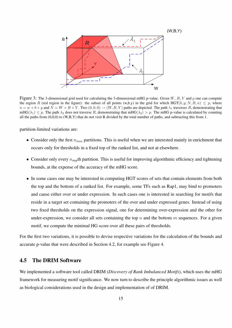
Figure 3: The 3-dimensional grid used for calculating the 3-dimensional mHG p-value. Given W , B, Y and p one can computethe region R (red region in the figure): the subset of all points (w,b,y) in the grid for which HGT(b, y;N,B, n) ≤ p, wheren = w + b + y and N = W + B + Y . Two (0, 0, 0) → (W,B, Y ) paths are depicted. The path λ1 traverses R, demonstrating thatmHG(λ1) ≤ p. The path λ2 does not traverse R, demonstrating that mHG(λ2) > p. The mHG p-value is calculated by countingall the paths from (0,0,0) to (W,B,Y) that do not visit R divided by the total number of paths, and subtracting this from 1.
partition-limited variations are:
• Consider only the first nmax partitions. This is useful when we are interested mainly in enrichment that
occurs only for thresholds in a fixed top of the ranked list, and not at elsewhere.
• Consider only every nstepth partition. This is useful for improving algorithmic efficiency and tightening
bounds, at the expense of the accuracy of the mHG score.
• In some cases one may be interested in computing HGT scores of sets that contain elements from both
the top and the bottom of a ranked list. For example, some TFs such as Rap1, may bind to promoters
and cause either over or under expression. In such cases one is interested in searching for motifs that
reside in a target set containing the promoters of the over and under expressed genes. Instead of using
two fixed thresholds on the expression signal, one for determining over-expression and the other for
under-expression, we consider all sets containing the top n and the bottom m sequences. For a given
motif, we compute the minimal HG score over all these pairs of thresholds.
For the first two variations, it is possible to devise respective variations for the calculation of the bounds and
accurate p-value that were described in Section 4.2, for example see Figure 4.
4.5 The DRIM Software
We implemented a software tool called DRIM (Discovery of Rank Imbalanced Motifs), which uses the mHG
framework for measuring motif significance. We now turn to describe the principle algorithmic issues as well
as biological considerations used in the design and implementation of of DRIM.
15
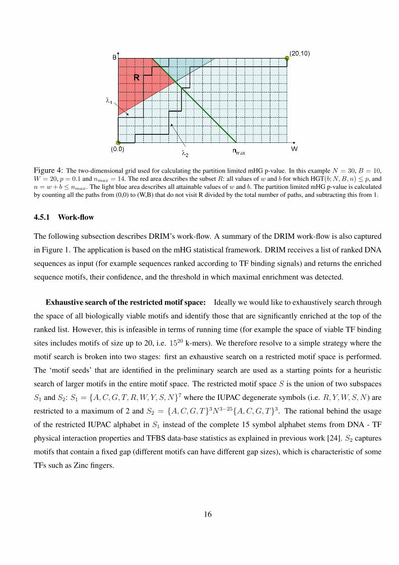
Figure 4: The two-dimensional grid used for calculating the partition limited mHG p-value. In this example N = 30, B = 10,W = 20, p = 0.1 and nmax = 14. The red area describes the subset R: all values of w and b for which HGT(b;N,B, n) ≤ p, andn = w + b ≤ nmax. The light blue area describes all attainable values of w and b. The partition limited mHG p-value is calculatedby counting all the paths from (0,0) to (W,B) that do not visit R divided by the total number of paths, and subtracting this from 1.
4.5.1 Work-flow
The following subsection describes DRIM’s work-flow. A summary of the DRIM work-flow is also captured
in Figure 1. The application is based on the mHG statistical framework. DRIM receives a list of ranked DNA
sequences as input (for example sequences ranked according to TF binding signals) and returns the enriched
sequence motifs, their confidence, and the threshold in which maximal enrichment was detected.
Exhaustive search of the restricted motif space: Ideally we would like to exhaustively search through
the space of all biologically viable motifs and identify those that are significantly enriched at the top of the
ranked list. However, this is infeasible in terms of running time (for example the space of viable TF binding
sites includes motifs of size up to 20, i.e. 1520 k-mers). We therefore resolve to a simple strategy where the
motif search is broken into two stages: first an exhaustive search on a restricted motif space is performed.
The ‘motif seeds’ that are identified in the preliminary search are used as a starting points for a heuristic
search of larger motifs in the entire motif space. The restricted motif space S is the union of two subspaces
S1 and S2: S1 = A, C,G, T, R, W, Y, S,N7 where the IUPAC degenerate symbols (i.e. R, Y,W, S, N ) are
restricted to a maximum of 2 and S2 = A, C,G, T3N3−25A, C,G, T3. The rational behind the usage
of the restricted IUPAC alphabet in S1 instead of the complete 15 symbol alphabet stems from DNA - TF
physical interaction properties and TFBS data-base statistics as explained in previous work [24]. S2 captures
motifs that contain a fixed gap (different motifs can have different gap sizes), which is characteristic of some
TFs such as Zinc fingers.
16

mHG enrichment: For each of the motifs in S we generate a ranked occurrence vector and compute the
enrichment in terms of the multi-dimensional mHG. Due to running time considerations we restrict the multi
dimensional mHG to 3 dimensions. This means that the model assumes each intergenic-region contains either
0, 1 or ≥2 copies of a motif. To test whether this assumption is reasonable in the case of true TFBS motifs
we examined the occurrence distribution of TFBS motifs that were experimentally verified in S. cerevisiae,
see Figure 5. It can be seen that the assumption holds for the 5 TFs that were tested since the majority of all
intergenic regions contained either 0, 1 or 2 copies of the TFBSs. At the end of this stage only motif seeds
with mHG score < 10−3 are kept (choice of threshold is explained in section 5.1). Similar motifs are filtered
(as explained in Section 4.5.5) and the remaining motif seeds are fed into the heuristic search module for
expansion, Figure 1iii-iv.
Motif expansion by heuristic search: The filtered motif seeds are used as starting points for identifica-
tion of larger motifs that do not reside in the restricted motif space. This is done through an iterative heuristic
process that employs simulated annealing. The objective function is to minimize the motif mHG p-value. We
tested two different strategies for determining valid moves in the motif space. In the first, we define a move
from motif M1 to M2 as valid if M1 and M2 are within a predefined Hamming distance D. All valid moves
are equiprobable. Additional bases can also be added to the motif flanks thus enabling motif expansion. Note
that the mHG adaptive cutoff is recalculated at each step. In the second strategy all the motif occurrences in
the target set that are within hamming distance D are aligned. A consensus motif above IUPAC is extracted
and the algorithm attempts to move to that motif. While the second strategy converges much faster than the
first it is also more prone to local minimum (in the final application we use the second strategy with D = 1). At
the end of the process the exact p-value of each of the expanded motifs is computed. To correct for multiple
motif testing the p-value is then multiplied by the motif space size. Only motifs with corrected p-value <
10−3 are reported.
Running time: The DRIM application has been implemented in C++. The “blind search” imposes that
over∼100, 000 motifs are checked for enrichment in each run. It is therefore paramount to optimize the above
procedures in order to enable a feasible running time. There are two bottlenecks in terms of running time: the
motif occurrence vector generation and the mHG computation. We developed several optimization schemes
to improve both (for details see Section 4.5.2 - 4.5.4). For example, running time on a list of 6000 sequences
with an average size of 480 bases is ∼3 minutes on a Pentium IV, 2 GHz, (a 3000 fold improvement over the
naive implementation (with out the optimizations) that took ∼9000 minutes per single run).
17
1
10
100
1000
10000
0 1 2 3 4 >5
TFBS occurrence multiplicity
Nu
mb
er
of
inte
rgen
ic r
eg
ion
s
BAS1
GAL4
CBF
INO2
LEU3
Figure 5: The distribution of TFBS occurrence multiplicities per intergenic region in Saccharomyces cerevisiae is shown for fiveTFs whose TFBS motif was experimentally verified. Note that the y-axis is logarithmic and that the fraction of sequences with 3or more occurrences is less than 0.1%.
4.5.2 How to compute the mHG score efficiently
Computing mHG in O(N · B) : Let N be the the size of a binary vector λ; B is the total number of
1’s in λ; b is the number of 1’s in λ1, ..., λn. A naive approach for computing the HG score at a fixed n
takes O(N) (see Equation 1). Consequentially, computing HGT takes O(N ·B) (see Equation 2). The mHG
score of λ can be computed by simply “sliding down” the vector and computing the HGT scores at each of
the N ranks yielding a time complexity of O(N2 · B). This strategy is inefficient in terms of running time,
especially in the context of motif finding where the mHG score is computed many times - for each motif in
the motif space. Another issue involves numerical errors that may arise in the computation of HG for large
N’s. To solve these issues some applications use the binomial distribution in order to approximate the HG
distribution [40].
We propose a strategy that circumvents the need for such approximations. Furthermore, we show how
to compute the HG and HGT scores in O(1) and O(B) respectively thus reducing the mHG computation to
O(N ·B). The idea is to slide down the vector and compute the HG score at position n + 1 using the already
known HG score at the previous position, n (see equations 9-11), as follows
The recursion base is:
HG(n = 0, b = 0, N,B) =
(00
)(NB
)(NB
) = 1, (9)
18

If entry n+1 in the vector is ’0’ then the HG score can be computed as follows:
HG(n + 1, b, B, N) = HG(n, b, B, N) · (n + 1)(N − n−B + b)
(n + 1− b)(N − n), (10)
If entry n+1 in the vector is ’1’ then the HG score can be computed as follows:
HG(n + 1, b + 1, B, N) = HG(n, b, B, N) · (n + 1)(B − b)
(b + 1)(N − n), (11)
While the above recursive formulas were developed for binary vectors, the same principle can be expanded to
vectors over higher dimensions. The recursive formulas for trinary vectors, as used by the DRIM application,
are given in Section 7.2.
Computing mHG in O(N + B2) : Another optimization of the mHG score computation takes advantage
of the following observation:
Theorem 4.1
n < m ⇒ HGT(b; N, B, n) ≤ HGT(b; N, B, m) (12)
Proof: Let Λ = 0, 1N be the space of binary vectors with B 1’s and N − B 0’s. bi is the number of 1’s
at the top i positions of a vector λ ∈ Λ and λ(i) ∈ 0, 1 is the value of the ith element of the vector. For any
n < m:
HGT(b; N, B, n) =|λ|bn(λ) ≥ b|
|Λ|≤ |
⋃mi=nλ|bi(λ) ≥ b|
|Λ|=|λ|bm(λ) ≥ b|
|Λ|= HGT(b; N, B, m).
(13)
This property can be used in order to improve the efficiency of the mHG score computation, especially when
N >> B. The idea is to compute the mHG only over partitions ni (1 ≤ i ≤ B) for which λ(ni) = 1
instead of minimizing over all possible N partitions (as in Equation 3). The above property guarantees that
the minimal HGT over these B partitions is equal to the minimal HGT score over all N partitions. This point
is illustrated in Figure 6. Since the computation of HGT is bounded by O(B) we can now compute the mHG
score in O(N +B2). In practice, the mHG computation can be further improved by using the partition limited
mHG variation explained in Section 4.4.
4.5.3 How to compute the mHG p-value efficiently
Devising the algorithm for computing the mHG p-value (Section 4.2) in terms of path counting is conceptually
convenient. However, such a strategy may become impractical in terms of computer precision for large
19
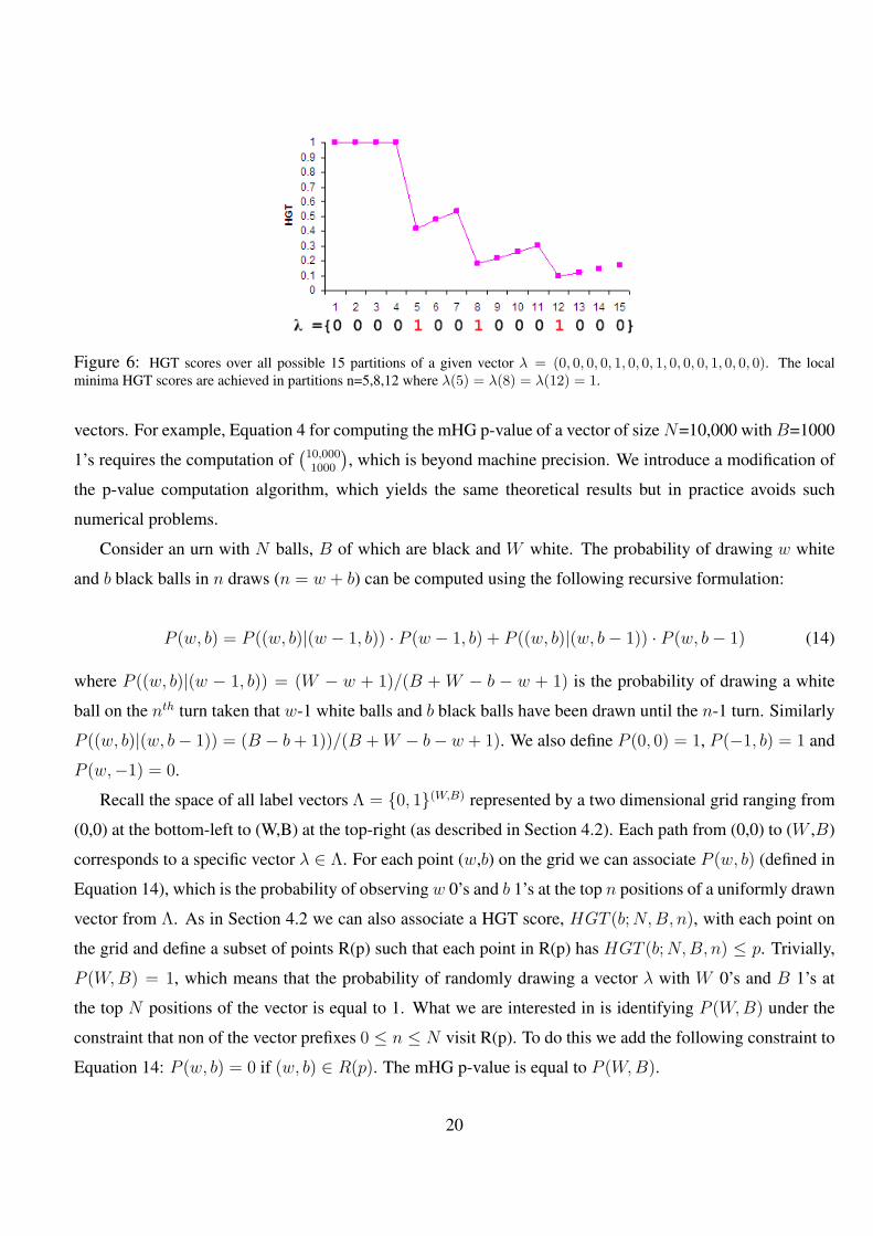
Figure 6: HGT scores over all possible 15 partitions of a given vector λ = (0, 0, 0, 0, 1, 0, 0, 1, 0, 0, 0, 1, 0, 0, 0). The localminima HGT scores are achieved in partitions n=5,8,12 where λ(5) = λ(8) = λ(12) = 1.
vectors. For example, Equation 4 for computing the mHG p-value of a vector of size N=10,000 with B=1000
1’s requires the computation of(10,0001000
), which is beyond machine precision. We introduce a modification of
the p-value computation algorithm, which yields the same theoretical results but in practice avoids such
numerical problems.
Consider an urn with N balls, B of which are black and W white. The probability of drawing w white
and b black balls in n draws (n = w + b) can be computed using the following recursive formulation:
P (w, b) = P ((w, b)|(w − 1, b)) · P (w − 1, b) + P ((w, b)|(w, b− 1)) · P (w, b− 1) (14)
where P ((w, b)|(w − 1, b)) = (W − w + 1)/(B + W − b − w + 1) is the probability of drawing a white
ball on the nth turn taken that w-1 white balls and b black balls have been drawn until the n-1 turn. Similarly
P ((w, b)|(w, b− 1)) = (B − b + 1))/(B + W − b− w + 1). We also define P (0, 0) = 1, P (−1, b) = 1 and
P (w,−1) = 0.
Recall the space of all label vectors Λ = 0, 1(W,B) represented by a two dimensional grid ranging from
(0,0) at the bottom-left to (W,B) at the top-right (as described in Section 4.2). Each path from (0,0) to (W ,B)
corresponds to a specific vector λ ∈ Λ. For each point (w,b) on the grid we can associate P (w, b) (defined in
Equation 14), which is the probability of observing w 0’s and b 1’s at the top n positions of a uniformly drawn
vector from Λ. As in Section 4.2 we can also associate a HGT score, HGT (b; N, B, n), with each point on
the grid and define a subset of points R(p) such that each point in R(p) has HGT (b; N, B, n) ≤ p. Trivially,
P (W, B) = 1, which means that the probability of randomly drawing a vector λ with W 0’s and B 1’s at
the top N positions of the vector is equal to 1. What we are interested in is identifying P (W, B) under the
constraint that non of the vector prefixes 0 ≤ n ≤ N visit R(p). To do this we add the following constraint to
Equation 14: P (w, b) = 0 if (w, b) ∈ R(p). The mHG p-value is equal to P (W, B).
20
Using the recursive formula in Equation 14 and a dynamic programming procedure the p-value can be
computed in O(W ·B). We note that the same principle is used for computing the multi-dimensional p-value.
4.5.4 Optimizing the occurrence vector generation
A straight forward strategy for generating the motif occurrence vector (MOV) is to exhaustively scan all
sequences and identify the number of motif occurrences in each sequence. Denote the total length of all
sequences N, and the size of the motif space M, than this strategy for constructing a MOV is bound by
O(MN). In practice M and N may be as large as large (M = ∼105, N = ∼107). Performing a motif search
on one ranked list takes approximately 9000 minutes on a Pentium IV, 2 GHz. Performing multiple runs
(as done in this study) becomes infeasible in terms of running time. To overcome this we exploit the fact
that the same set of sequences is often used in different experiments. As a preprocessing step we construct
a lookup table that maps motif prefixes of size m with their locations in the sequences. Given such a table,
constructing a MOV of a motif of size m′ (where m′ ≥ m) can be done by searching for motif occurrences
only at locations where the corresponding motif prefix appears. The approximate running time improvement
(assuming equiprobable nucleotide distribution) is (1/4)m. In practice we use m = 7. This idea was further
expanded to deal with motifs that contain IUPAC symbols.
4.5.5 Measuring motif similarity
Devising a motif similarity measure is important in order to enable a quantitative comparison between our
predicted motifs to those reported in other studies. This measure is also useful for filtering similar motifs as
performed by DRIM. First, we define a similarity measure between IUPAC symbols. Let α and β be symbols
over the IUPAC alphabet - α, β ∈ A, C, G, T , R, Y , W , S, M , K, H , B, V , D, N. Each IUPAC symbol
can also be represented by a specific subset over A, C, G, T. We define a distance between α and β as
follows:
δ(α, β) = 1− 2|α ∩ β||α|+ |β|
. (15)
Notice that this metric maintains the following properties:
1. For identical symbols δ(α, β) = 0 (i.e. identical symbols have a distance of 0) ;
2. For disjoint symbols δ(α, β) = 1 (e.g. A vs. C or W = A, T vs. S = C, G) ;
3. 0 ≤ δ(α, β) ≤ 1 (e.g. α=A, C,G, β=A, G → δ(α, β) = 0.2) .
21
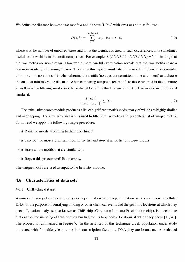
We define the distance between two motifs a and b above IUPAC with sizes m and n as follows:
D(a, b) =
min(n,m)∑i=1
δ(ai, bi) + w1u, (16)
where u is the number of unpaired bases and w1 is the weight assigned to such occurrences. It is sometimes
useful to allow shifts in the motif comparison. For example, D(ACGTAC, CGTACG) = 6, indicating that
the two motifs are non-similar. However, a more careful examination reveals that the two motifs share a
common substring containing 5 bases. To capture this type of similarity in the motif comparison we consider
all n + m − 1 possible shifts when aligning the motifs (no gaps are permitted in the alignment) and choose
the one that minimizes the distance. When comparing our predicted motifs to those reported in the literature
as well as when filtering similar motifs produced by our method we use w1 = 0.6. Two motifs are considered
similar if:D(a, b)
mean(|a|, |b|)≤ 0.5. (17)
The exhaustive search module produces a list of significant motifs seeds, many of which are highly similar
and overlapping. The similarity measure is used to filter similar motifs and generate a list of unique motifs.
To this end we apply the following simple procedure:
(i) Rank the motifs according to their enrichment
(i) Take out the most significant motif in the list and store it in the list of unique motifs
(ii) Erase all the motifs that are similar to it
(iii) Repeat this process until list is empty.
The unique motifs are used as input to the heuristic module.
4.6 Characteristics of data sets
4.6.1 ChIP-chip dataset
A number of assays have been recently developed that use immunopercipitation based enrichment of cellular
DNA for the purpose of identifying binding or other chemical events and the genomic locations at which they
occur. Location analysis, also known as ChIP-chip (Chromatin Immuno-Precipitation chip), is a technique
that enables the mapping of transcription binding events to genomic locations at which they occur [11, 41].
The process is summarized in Figure 7. In the first step of this technique a cell population under study
is treated with formaldehyde to cross-link transcription factors to DNA they are bound to. A sonicated
22
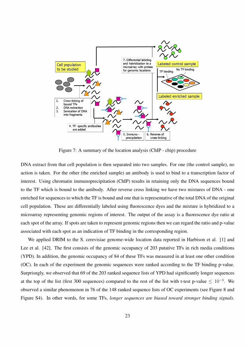
Figure 7: A summary of the location analysis (ChIP - chip) procedure
DNA extract from that cell population is then separated into two samples. For one (the control sample), no
action is taken. For the other (the enriched sample) an antibody is used to bind to a transcription factor of
interest. Using chromatin immunoprecipitation (ChIP) results in retaining only the DNA sequences bound
to the TF which is bound to the antibody. After reverse cross linking we have two mixtures of DNA - one
enriched for sequences to which the TF is bound and one that is representative of the total DNA of the original
cell population. These are differentially labeled using fluorescence dyes and the mixture is hybridized to a
microarray representing genomic regions of interest. The output of the assay is a fluorescence dye ratio at
each spot of the array. If spots are taken to represent genomic regions then we can regard the ratio and p-value
associated with each spot as an indication of TF binding in the corresponding region.
We applied DRIM to the S. cerevisiae genome-wide location data reported in Harbison et al. [1] and
Lee et al. [42]. The first consists of the genomic occupancy of 203 putative TFs in rich media conditions
(YPD). In addition, the genomic occupancy of 84 of these TFs was measured in at least one other condition
(OC). In each of the experiment the genomic sequences were ranked according to the TF binding p-value.
Surprisngly, we observed that 69 of the 203 ranked sequence lists of YPD had significantly longer sequences
at the top of the list (first 300 sequences) compared to the rest of the list with t-test p-value ≤ 10−3. We
observed a similar phenomenon in 76 of the 148 ranked sequence lists of OC experiments (see Figure 8 and
Figure S4). In other words, for some TFs, longer sequences are biased toward stronger binding signals.
23
This observation is unexpected since, although longer probes hybridize more labeled material than shorter
probes the increase should be proportional in both channels. This type of length bias may cause spurious
results under our model assumptions and hence the final dataset, termed ‘Harbison filtered dataset’, refers
to the remaining 207 experiments (135 YPD, and 72 OC) of 162 unique TFs that did not have length bias
(Supplementary Table S1).
An additional ChIP-chip data set was constructed using the data reported in Lee et al. [42] containing
113 experiments in rich media. The data is partially exclusive to the data of Harbison et al. [1]. The same
filtering procedure was performed, resulting in a set of 65 experiments, termed ‘Lee filtered dataset’.
Figure 8: Sequence length bias observed in ChIP-chip data of the TF MSN2 measured in an acidic condition. The yeast intergenicregions were ranked according to their binding to MSN2, (strong to weak binding appear from left to right). The figure shows thesequence lengths at each rank. The red trend line (a moving average of 200) indicates that sequences that are ranked higher interms of TF binding are also longer. A student t-test comparing the lengths of the top 300 versus the rest of the sequences yieldeda highly significant p-value ≤ 10−40.
4.6.2 Methylated CpG dataset
Using a technique similar to ChIP-chip, termed methyl-DNA immunoprecipitation (mDIP), enables the mea-
surement of methylated CpG island patterns [43, 6]. The third dataset contains the CpG island methylation
patterns of 4 different human cancer cell-lines (Caco-2, Polyp, Carcinoma, PC3) where several replicate ex-
periments were done for each of the cell-lines. In each of these experiments the CpG methylation signal was
measured in ∼ 13,000 gene promoters as reported in [6].
24
5 Results
5.1 Proof of principle
We begin by testing our method on synthetically generated clear-cut positive and negative control cases. We
do this in order to verify that DRIM accurately identifies motifs in well characterized and experimentally
verified examples and at the same time avoids false identification of motifs in randomly ordered genomic
sequences. The latter objective is of particular importance since the issue of false identification has been
mentioned as one of the main shortcomings of motif discovery approaches. For example, in a previous study
six different motif discovery applications were used to search for TFBS motifs [1]. Each of the programs
attempted to measure the significance of its results using one or more enrichment scores. The authors report
that the applications outputted high-scoring motifs even when applied to random selections of intergenic
regions. In another work the authors generated clusters of genes whose expression patterns correlate to the
expression of a particular TF [44]. These clusters were then analyzed for enriched motifs. Again, the authors
report that random sets, with sizes matching those of the real clusters, contained a large number of motifs
with significant scores.
To test our method’s false prediction rate we performed the following negative control experiment: 5
different random permutations of ChIP-chip data were generated by randomly selecting 400 promoters and
randomly permuting their ranks. DRIM was then applied to these sets and scanned over ∼100,000 different
motifs in each set. None of the motifs that were scanned had a significant corrected mHG p-value < 10−3.
Note that in order to get the corrected p-values two levels of multiple test corrections are performed: correct-
ing for the number motifs that are tested and correcting for multiple cutoffs that are tested as part of the mHG
optimization process. In section 5.5 we describe a comparison to other methods using the same random set
benchmarking.
How do the p-values of random motifs compare to those of true biological motifs? To test this we chose
5 TFs (BAS1, GAL4, CBF1, INO2 and LEU3) whose motif binding sites are well characterized and experi-
mentally verified. We applied DRIM to the ChIP-chip data of these TFs as reported in [1]. In all instances the
true motifs were identified with corrected p-values of 10−6, 10−9, 10−76, 10−18, 10−8 respectively. A com-
parison of the p-value distribution of the motifs in the randomly ordered sequences with that of the verified
TFBS motifs is given in Figure 9. In all instances the true TFBS motifs were predicted with p-values that
were several orders of magnitude more significant than the best p-value of a motif in the randomly permuted
data. This indicates that the enrichment signals of true TFBS, as captured by the mHG p-value, are clearly
distinct from the signals we expect to find in random rankings of genomic sequences.
25
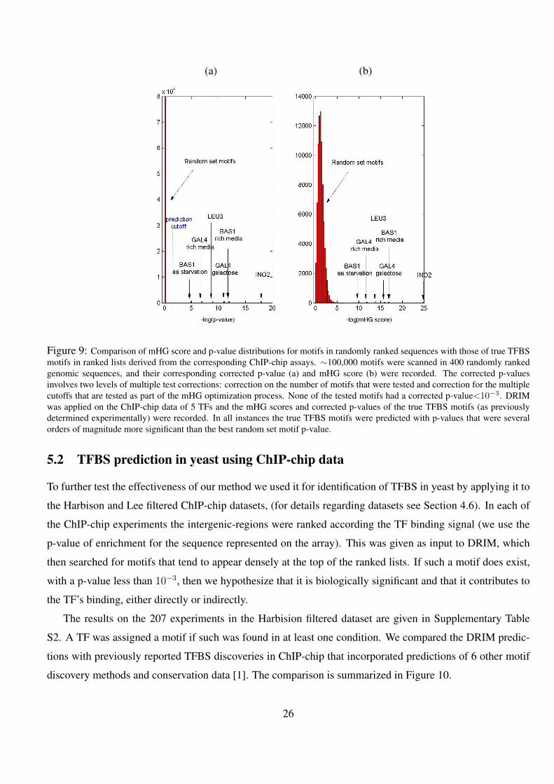
(a) (b)
Figure 9: Comparison of mHG score and p-value distributions for motifs in randomly ranked sequences with those of true TFBSmotifs in ranked lists derived from the corresponding ChIP-chip assays. ∼100,000 motifs were scanned in 400 randomly rankedgenomic sequences, and their corresponding corrected p-value (a) and mHG score (b) were recorded. The corrected p-valuesinvolves two levels of multiple test corrections: correction on the number of motifs that were tested and correction for the multiplecutoffs that are tested as part of the mHG optimization process. None of the tested motifs had a corrected p-value<10−3. DRIMwas applied on the ChIP-chip data of 5 TFs and the mHG scores and corrected p-values of the true TFBS motifs (as previouslydetermined experimentally) were recorded. In all instances the true TFBS motifs were predicted with p-values that were severalorders of magnitude more significant than the best random set motif p-value.
5.2 TFBS prediction in yeast using ChIP-chip data
To further test the effectiveness of our method we used it for identification of TFBS in yeast by applying it to
the Harbison and Lee filtered ChIP-chip datasets, (for details regarding datasets see Section 4.6). In each of
the ChIP-chip experiments the intergenic-regions were ranked according the TF binding signal (we use the
p-value of enrichment for the sequence represented on the array). This was given as input to DRIM, which
then searched for motifs that tend to appear densely at the top of the ranked lists. If such a motif does exist,
with a p-value less than 10−3, then we hypothesize that it is biologically significant and that it contributes to
the TF’s binding, either directly or indirectly.
The results on the 207 experiments in the Harbision filtered dataset are given in Supplementary Table
S2. A TF was assigned a motif if such was found in at least one condition. We compared the DRIM predic-
tions with previously reported TFBS discoveries in ChIP-chip that incorporated predictions of 6 other motif
discovery methods and conservation data [1]. The comparison is summarized in Figure 10.
26
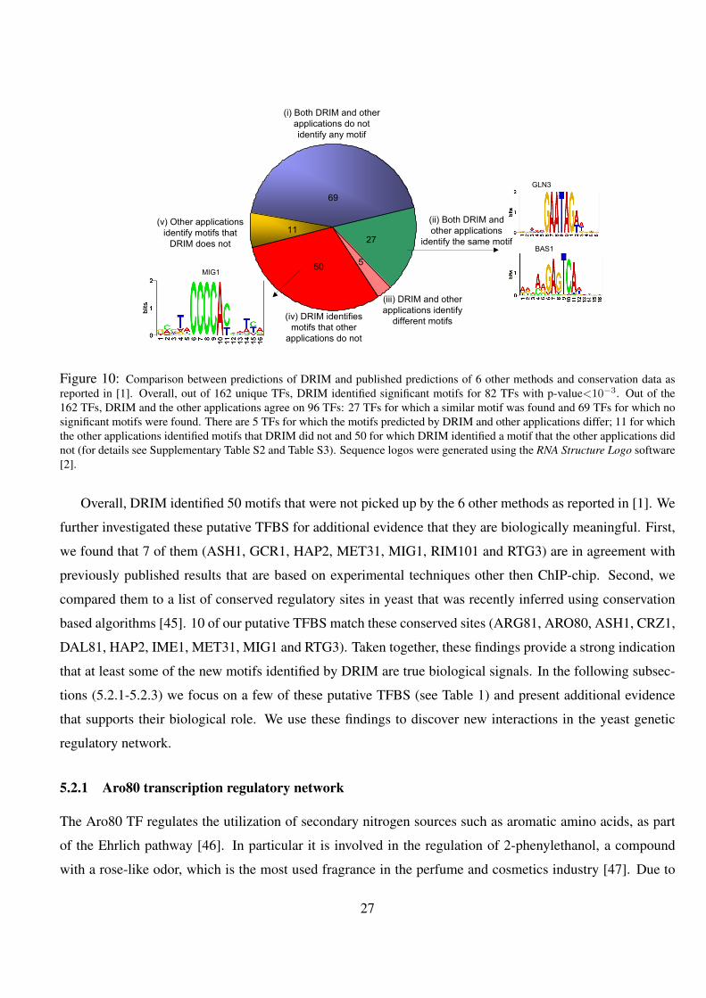
(i) Both DRIM and other
applications do not
identify any motif
(ii) Both DRIM and
other applications
identify the same motif
(iii) DRIM and other
applications identify
different motifs(iv) DRIM identifies
motifs that other
applications do not
(v) Other applications
identify motifs that
DRIM does not
50
69
5
2711
BAS1
GLN3
MIG1
Figure 10: Comparison between predictions of DRIM and published predictions of 6 other methods and conservation data asreported in [1]. Overall, out of 162 unique TFs, DRIM identified significant motifs for 82 TFs with p-value<10−3. Out of the162 TFs, DRIM and the other applications agree on 96 TFs: 27 TFs for which a similar motif was found and 69 TFs for which nosignificant motifs were found. There are 5 TFs for which the motifs predicted by DRIM and other applications differ; 11 for whichthe other applications identified motifs that DRIM did not and 50 for which DRIM identified a motif that the other applications didnot (for details see Supplementary Table S2 and Table S3). Sequence logos were generated using the RNA Structure Logo software[2].
Overall, DRIM identified 50 motifs that were not picked up by the 6 other methods as reported in [1]. We
further investigated these putative TFBS for additional evidence that they are biologically meaningful. First,
we found that 7 of them (ASH1, GCR1, HAP2, MET31, MIG1, RIM101 and RTG3) are in agreement with
previously published results that are based on experimental techniques other then ChIP-chip. Second, we
compared them to a list of conserved regulatory sites in yeast that was recently inferred using conservation
based algorithms [45]. 10 of our putative TFBS match these conserved sites (ARG81, ARO80, ASH1, CRZ1,
DAL81, HAP2, IME1, MET31, MIG1 and RTG3). Taken together, these findings provide a strong indication
that at least some of the new motifs identified by DRIM are true biological signals. In the following subsec-
tions (5.2.1-5.2.3) we focus on a few of these putative TFBS (see Table 1) and present additional evidence
that supports their biological role. We use these findings to discover new interactions in the yeast genetic
regulatory network.
5.2.1 Aro80 transcription regulatory network
The Aro80 TF regulates the utilization of secondary nitrogen sources such as aromatic amino acids, as part
of the Ehrlich pathway [46]. In particular it is involved in the regulation of 2-phenylethanol, a compound
with a rose-like odor, which is the most used fragrance in the perfume and cosmetics industry [47]. Due to
27
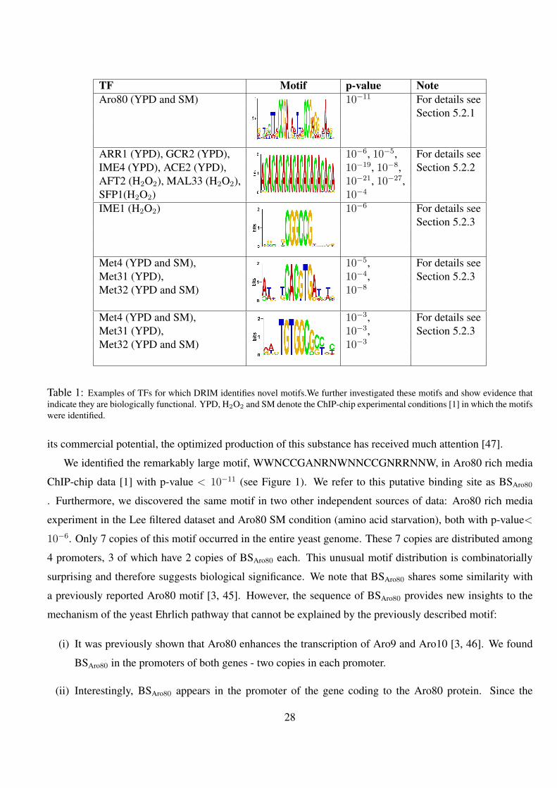
TF Motif p-value NoteAro80 (YPD and SM) 10−11 For details see
Section 5.2.1
ARR1 (YPD), GCR2 (YPD), 10−6, 10−5, For details seeIME4 (YPD), ACE2 (YPD), 10−19, 10−8, Section 5.2.2AFT2 (H2O2), MAL33 (H2O2), 10−21, 10−27,SFP1(H2O2) 10−4
IME1 (H2O2) 10−6 For details seeSection 5.2.3
Met4 (YPD and SM), 10−5, For details seeMet31 (YPD), 10−4, Section 5.2.3Met32 (YPD and SM) 10−8
Met4 (YPD and SM), 10−3, For details seeMet31 (YPD), 10−3, Section 5.2.3Met32 (YPD and SM) 10−3
Table 1: Examples of TFs for which DRIM identifies novel motifs.We further investigated these motifs and show evidence thatindicate they are biologically functional. YPD, H2O2 and SM denote the ChIP-chip experimental conditions [1] in which the motifswere identified.
its commercial potential, the optimized production of this substance has received much attention [47].
We identified the remarkably large motif, WWNCCGANRNWNNCCGNRRNNW, in Aro80 rich media
ChIP-chip data [1] with p-value < 10−11 (see Figure 1). We refer to this putative binding site as BSAro80
. Furthermore, we discovered the same motif in two other independent sources of data: Aro80 rich media
experiment in the Lee filtered dataset and Aro80 SM condition (amino acid starvation), both with p-value<
10−6. Only 7 copies of this motif occurred in the entire yeast genome. These 7 copies are distributed among
4 promoters, 3 of which have 2 copies of BSAro80 each. This unusual motif distribution is combinatorially
surprising and therefore suggests biological significance. We note that BSAro80 shares some similarity with
a previously reported Aro80 motif [3, 45]. However, the sequence of BSAro80 provides new insights to the
mechanism of the yeast Ehrlich pathway that cannot be explained by the previously described motif:
(i) It was previously shown that Aro80 enhances the transcription of Aro9 and Aro10 [3, 46]. We found
BSAro80 in the promoters of both genes - two copies in each promoter.
(ii) Interestingly, BSAro80 appears in the promoter of the gene coding to the Aro80 protein. Since the
28
BSAro80 motif appears only in 4 promoters in the entire genome it is highly unlikely that this occurred
by chance. We therefore hypothesize that Aro80 self-regulates its own transcription by directly binding
to its own promoter.
(iii) The fourth promoter (when ranking according to Aro80 rich media ChIP-chip data [1]) contains two
BSAro80 elements, one on the sense and the other on the anti-sense. This configuration is shared by
two divergently transcribed genes, NAF1 and Esbp6. The latter gene was previously shown to have
increased transcription in the presence of phenylalanine as sole nitrogen source [46], suggesting it may
play a role in the Ehrlich pathway. Esbp6 is a monocarboxylate permease and might be involved in the
transfer of substrates of the Ehrlich pathway across the plasma membrane
(iv) We analyzed the conservation of BSAro80 in 4 yeast strains and found all 7 of its copies to be conserved
in the different strains.
(v) Aro80 belongs to the Zn2Cys6 family of TFs that are known to bind CCG elements separated by
a spacing. Indeed, in addition to other conserved nucleotides the motif contains CCG gapped tri-
nucleotides.
(vi) In a previous study, in order to identify cis-acting sequences involved in Aro9 induction, a series of
deletions were produced in the Aro9 promoter region and the expression of a reporter gene was moni-
tored [3]. The authors concluded that the sequence CCGN7CCGN7CCGN7CCG in the Aro9 promoter
is responsible for Aro80 binding. We note, however, that the changes in expression caused by the
mutations can be interpreted differently and in fact they are even more consistent with our BSAro80
motif. Deletions or mutations that simultaneously altered all motif copies in the promoter dramatically
reduced expression, while those which altered only some of the copies caused a more mild decrease.
Other deletions that did not affect any BSAro80 motif did not affect the expression at all. A detailed
analysis of the BSAro80 element in respect to these mutagenesis studies is given in Figure 12.
A putative transcription network of Aro80 that incorporates these findings is shown in Figure 11a. Another
interesting observation is that adjacent to the BSAro80 motif there are three GATA binding sites (see Figure
11b). We used these findings (and other information) to further hypothesize on the mechanism by which the
Aro80 pathway is regulated (for details see Section 7.4).
The predicted motif BSAro80 exemplifies the usefulness of the mHG flexible cutoff. Our process parti-
tioned the data into a target set containing the top first 4 promoters (the only promoters in the genome in
which the motif resides) and a background set containing the rest of the promoters. Other methods that used
a fixed binding signal cutoff (p-value< 10−3) for partitioning the data included 16 other promoters in the
29
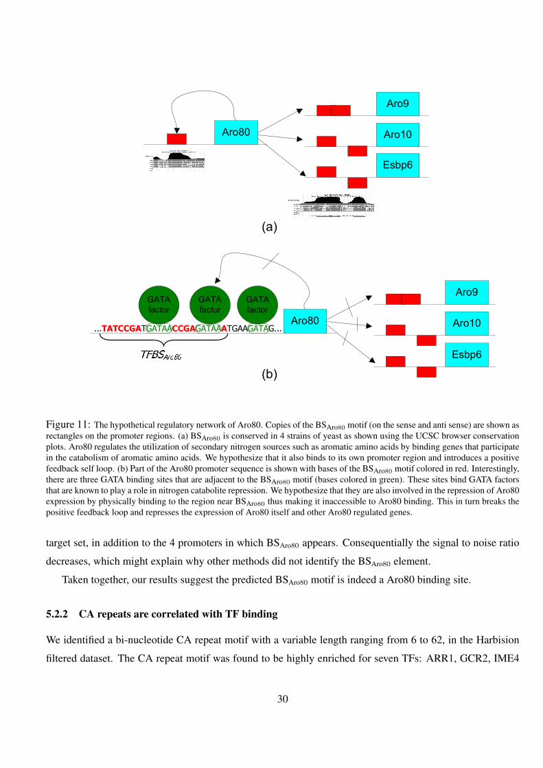
Aro10
Esbp6
Aro80
Aro9
(a)
(b)
...TATCCGATGATAACCGAGATAAATGAAGATAG...
GATA
factor
Aro10
Esbp6
Aro80
Aro9GATA
factor
GATA
factor
Figure 11: The hypothetical regulatory network of Aro80. Copies of the BSAro80 motif (on the sense and anti sense) are shown asrectangles on the promoter regions. (a) BSAro80 is conserved in 4 strains of yeast as shown using the UCSC browser conservationplots. Aro80 regulates the utilization of secondary nitrogen sources such as aromatic amino acids by binding genes that participatein the catabolism of aromatic amino acids. We hypothesize that it also binds to its own promoter region and introduces a positivefeedback self loop. (b) Part of the Aro80 promoter sequence is shown with bases of the BSAro80 motif colored in red. Interestingly,there are three GATA binding sites that are adjacent to the BSAro80 motif (bases colored in green). These sites bind GATA factorsthat are known to play a role in nitrogen catabolite repression. We hypothesize that they are also involved in the repression of Aro80expression by physically binding to the region near BSAro80 thus making it inaccessible to Aro80 binding. This in turn breaks thepositive feedback loop and represses the expression of Aro80 itself and other Aro80 regulated genes.
target set, in addition to the 4 promoters in which BSAro80 appears. Consequentially the signal to noise ratio
decreases, which might explain why other methods did not identify the BSAro80 element.
Taken together, our results suggest the predicted BSAro80 motif is indeed a Aro80 binding site.
5.2.2 CA repeats are correlated with TF binding
We identified a bi-nucleotide CA repeat motif with a variable length ranging from 6 to 62, in the Harbision
filtered dataset. The CA repeat motif was found to be highly enriched for seven TFs: ARR1, GCR2, IME4
30
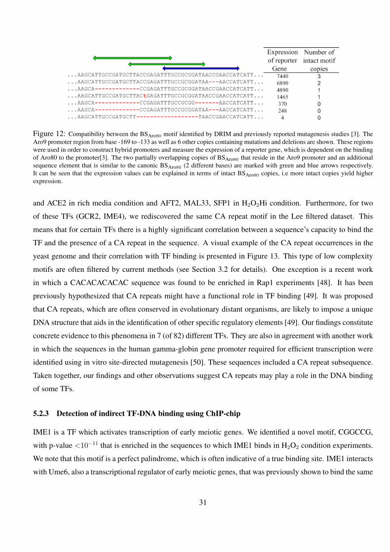
Figure 12: Compatibility between the BSAro80 motif identified by DRIM and previously reported mutagenesis studies [3]. TheAro9 promoter region from base -169 to -133 as well as 6 other copies containing mutations and deletions are shown. These regionswere used in order to construct hybrid promoters and measure the expression of a reporter gene, which is dependent on the bindingof Aro80 to the promoter[3]. The two partially overlapping copies of BSAro80 that reside in the Aro9 promoter and an additionalsequence element that is similar to the canonic BSAro80 (2 different bases) are marked with green and blue arrows respectively.It can be seen that the expression values can be explained in terms of intact BSAro80 copies, i.e more intact copies yield higherexpression.
and ACE2 in rich media condition and AFT2, MAL33, SFP1 in H2O2Hi condition. Furthermore, for two
of these TFs (GCR2, IME4), we rediscovered the same CA repeat motif in the Lee filtered dataset. This
means that for certain TFs there is a highly significant correlation between a sequence’s capacity to bind the
TF and the presence of a CA repeat in the sequence. A visual example of the CA repeat occurrences in the
yeast genome and their correlation with TF binding is presented in Figure 13. This type of low complexity
motifs are often filtered by current methods (see Section 3.2 for details). One exception is a recent work
in which a CACACACACAC sequence was found to be enriched in Rap1 experiments [48]. It has been
previously hypothesized that CA repeats might have a functional role in TF binding [49]. It was proposed
that CA repeats, which are often conserved in evolutionary distant organisms, are likely to impose a unique
DNA structure that aids in the identification of other specific regulatory elements [49]. Our findings constitute
concrete evidence to this phenomena in 7 (of 82) different TFs. They are also in agreement with another work
in which the sequences in the human gamma-globin gene promoter required for efficient transcription were
identified using in vitro site-directed mutagenesis [50]. These sequences included a CA repeat subsequence.
Taken together, our findings and other observations suggest CA repeats may play a role in the DNA binding
of some TFs.
5.2.3 Detection of indirect TF-DNA binding using ChIP-chip
IME1 is a TF which activates transcription of early meiotic genes. We identified a novel motif, CGGCCG,
with p-value <10−11 that is enriched in the sequences to which IME1 binds in H2O2 condition experiments.
We note that this motif is a perfect palindrome, which is often indicative of a true binding site. IME1 interacts
with Ume6, also a transcriptional regulator of early meiotic genes, that was previously shown to bind the same
31
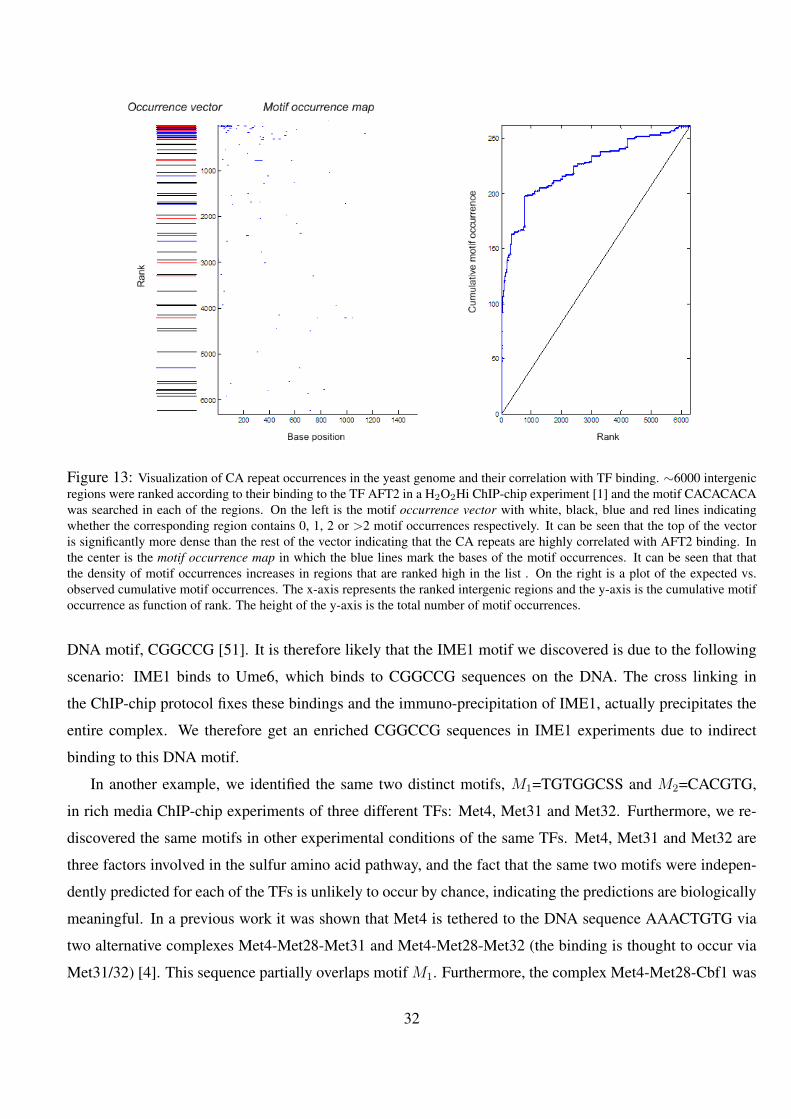
Figure 13: Visualization of CA repeat occurrences in the yeast genome and their correlation with TF binding. ∼6000 intergenicregions were ranked according to their binding to the TF AFT2 in a H2O2Hi ChIP-chip experiment [1] and the motif CACACACAwas searched in each of the regions. On the left is the motif occurrence vector with white, black, blue and red lines indicatingwhether the corresponding region contains 0, 1, 2 or >2 motif occurrences respectively. It can be seen that the top of the vectoris significantly more dense than the rest of the vector indicating that the CA repeats are highly correlated with AFT2 binding. Inthe center is the motif occurrence map in which the blue lines mark the bases of the motif occurrences. It can be seen that thatthe density of motif occurrences increases in regions that are ranked high in the list . On the right is a plot of the expected vs.observed cumulative motif occurrences. The x-axis represents the ranked intergenic regions and the y-axis is the cumulative motifoccurrence as function of rank. The height of the y-axis is the total number of motif occurrences.
DNA motif, CGGCCG [51]. It is therefore likely that the IME1 motif we discovered is due to the following
scenario: IME1 binds to Ume6, which binds to CGGCCG sequences on the DNA. The cross linking in
the ChIP-chip protocol fixes these bindings and the immuno-precipitation of IME1, actually precipitates the
entire complex. We therefore get an enriched CGGCCG sequences in IME1 experiments due to indirect
binding to this DNA motif.
In another example, we identified the same two distinct motifs, M1=TGTGGCSS and M2=CACGTG,
in rich media ChIP-chip experiments of three different TFs: Met4, Met31 and Met32. Furthermore, we re-
discovered the same motifs in other experimental conditions of the same TFs. Met4, Met31 and Met32 are
three factors involved in the sulfur amino acid pathway, and the fact that the same two motifs were indepen-
dently predicted for each of the TFs is unlikely to occur by chance, indicating the predictions are biologically
meaningful. In a previous work it was shown that Met4 is tethered to the DNA sequence AAACTGTG via
two alternative complexes Met4-Met28-Met31 and Met4-Met28-Met32 (the binding is thought to occur via
Met31/32) [4]. This sequence partially overlaps motif M1. Furthermore, the complex Met4-Met28-Cbf1 was
32

shown to bind motif M2 [5]. Previous findings are summarized in Figure 14a. The above explains why we
predict M1 for Met4 and M2 for Met31/32. However, it does not explain why we also predict M2 for Met4
and M1 for Met31/32. The most likely explanation for this is the existence of a direct interaction between the
two complexes Met4-Met28-Cbf1 and Met4-Met28-Met31/32. If such an interaction exists then the cross-
linking would fix the two complexes and cause the immuno-precipitation of either Met4, Met31 and Met32 to
precipitate the same set of sequences thus causing the same motifs to appear in the experiments of all 3 TFs,
which is exactly what DRIM identifies. This point is illustrated in Figure 14b. The idea of direct interaction
between the two complexes is also in agreement with a previous work [4].
Overall the results shown in this subsection demonstrate that DRIM is able to pick up on previously
ignored subtle signals in ChIP-chip data that stem from indirect bindings of factors to DNA. This type of
information can be useful for inferring novel protein-protein interactions.
(a)
(b)
Figure 14: (a) Schematic representation of Met4-Met28-CBF and Met4-Met28-Met31/32 complexes [4, 5]. (b) A hypotheticalMet4-Met28-CBF-Met31/32 complex. Immuno-precipitation of any of the TFs in the complex will precipitate the same set ofsequences, which explains why DRIM identifies the same two motifs for all TFs in the complex.
5.2.4 Condition dependent motifs
A comparison was made between the predicted motifs of the same TF in different experimental conditions
(see Table S2). These seem to fall into two main categories: (i) motifs whose enrichment is condition de-
pendent and (ii) motifs whose enrichment is condition invariant, suggesting the TF is bound to the DNA
regardless of condition. In the latter, although the same motif was predicted in different conditions the motif
enrichment varied considerably. For instance, the GAL4 binding site CGGN11CCG, previously reported in
[11] and other literature, was predicted in both YPD and galactose conditions. However, the enrichment
33
varied considerably with p-values 10−7 and 10−11, respectively. This several fold difference in enrichment is
consistent with what is known about the role of GAL4 in galactose metabolism. It suggests that GAL4 has
a preference to bind CGGN11CCG DNA regardless of condition. However, in the presence of galactose and
absence of glucose, this preference becomes much more significant. Another example of a condition invariant
motif whose binding strength is subject to experimental condition is that of Aro80, see section 5.2.1.
This demonstrates that DRIM can be used not only to identify binding sites but also to distinguish between
different modes of TF binding.
5.3 Motif discovery in Human methylated CpG islands
We turn to examine our method’s ability to predict sequence motifs that stem from data other than TF binding.
To this end, DRIM was applied to the dataset containing the human cancer cell-line methylated CpG islands
(for dataset details see Section 4.6.2) in order to try and identify motifs that are enriched in hyper methylated
regions. The promoters were ranked according to their methylation signal, hyper-methylated promoters at
the top. Note that different replicates of the same cell-line may yield different ranking of the promoters.
DRIM identified significantly enriched motifs in each of the 4 cancer cell-lines. Table 2 shows all the
motifs that were independently discovered in at least 2 different replicates of the same experiment or are in
agreement with previous work [6]. Overall, DRIM discovered 13 motifs: 10 novel motifs and 3 that have
been previously predicted in hyper methylated CpG island promoters in the same cancer cell-lines [6]. Some
of these motifs have also been independently identified in methyled CpG regions of other cell-lines [52, 53].
Remarkably, 9 of the novel 10 motifs have been identified in DNA regions to which the proteins of the
Polycomb complex bind [8, 9, 54]. The Polycomb complex is involved in gene repression through epigenetic
silencing and chromatin remodeling, a process that involves histone methylation. The fact that these two
distinct key epigenetic repression systems, namely histone methylation and CpG methylation, bind to regions
that share a similar set of sequence motifs suggests they are linked. To further establish this link we applied
DRIM to Polycomb complex bound promoters in human embriyonic fibroblasts [10]. We found 4 motifs
that are similar to the CpG methylation motifs (Table 2). Our findings are consistent with a recent paper that
showed that the EZH2 protein binds methyltransferases via the a Polycomb complex [55].
We note that most of the motifs we found are similar across more than one type of cancer-cells, e.g.
variants of the GCTGCT motif appear in both Caco-2, PC3 and Polyp1. This suggests that the same DNA
binding factors are involved in CpG methylation of different types of cancer-cells. It is also important to
note that some of the motifs we discovered are G-C rich. The enrichment of these motifs may be partially
attributed to the G-C content bias that is found in the CpG methylation data. Interestingly, some of the motifs
we found to be correlated with CpG methylation are low complexity motifs such as the CA repeat and GA
34
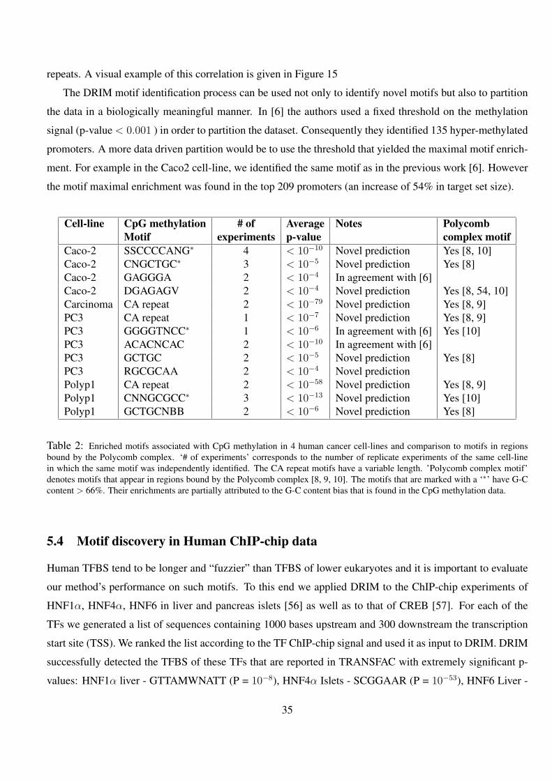
repeats. A visual example of this correlation is given in Figure 15
The DRIM motif identification process can be used not only to identify novel motifs but also to partition
the data in a biologically meaningful manner. In [6] the authors used a fixed threshold on the methylation
signal (p-value < 0.001 ) in order to partition the dataset. Consequently they identified 135 hyper-methylated
promoters. A more data driven partition would be to use the threshold that yielded the maximal motif enrich-
ment. For example in the Caco2 cell-line, we identified the same motif as in the previous work [6]. However
the motif maximal enrichment was found in the top 209 promoters (an increase of 54% in target set size).
Cell-line CpG methylation # of Average Notes PolycombMotif experiments p-value complex motif
Caco-2 SSCCCCANG∗ 4 < 10−10 Novel prediction Yes [8, 10]Caco-2 CNGCTGC∗ 3 < 10−5 Novel prediction Yes [8]Caco-2 GAGGGA 2 < 10−4 In agreement with [6]Caco-2 DGAGAGV 2 < 10−4 Novel prediction Yes [8, 54, 10]Carcinoma CA repeat 2 < 10−79 Novel prediction Yes [8, 9]PC3 CA repeat 1 < 10−7 Novel prediction Yes [8, 9]PC3 GGGGTNCC∗ 1 < 10−6 In agreement with [6] Yes [10]PC3 ACACNCAC 2 < 10−10 In agreement with [6]PC3 GCTGC 2 < 10−5 Novel prediction Yes [8]PC3 RGCGCAA 2 < 10−4 Novel predictionPolyp1 CA repeat 2 < 10−58 Novel prediction Yes [8, 9]Polyp1 CNNGCGCC∗ 3 < 10−13 Novel prediction Yes [10]Polyp1 GCTGCNBB 2 < 10−6 Novel prediction Yes [8]
Table 2: Enriched motifs associated with CpG methylation in 4 human cancer cell-lines and comparison to motifs in regionsbound by the Polycomb complex. ‘# of experiments’ corresponds to the number of replicate experiments of the same cell-linein which the same motif was independently identified. The CA repeat motifs have a variable length. ’Polycomb complex motif’denotes motifs that appear in regions bound by the Polycomb complex [8, 9, 10]. The motifs that are marked with a ‘∗’ have G-Ccontent > 66%. Their enrichments are partially attributed to the G-C content bias that is found in the CpG methylation data.
5.4 Motif discovery in Human ChIP-chip data
Human TFBS tend to be longer and “fuzzier” than TFBS of lower eukaryotes and it is important to evaluate
our method’s performance on such motifs. To this end we applied DRIM to the ChIP-chip experiments of
HNF1α, HNF4α, HNF6 in liver and pancreas islets [56] as well as to that of CREB [57]. For each of the
TFs we generated a list of sequences containing 1000 bases upstream and 300 downstream the transcription
start site (TSS). We ranked the list according to the TF ChIP-chip signal and used it as input to DRIM. DRIM
successfully detected the TFBS of these TFs that are reported in TRANSFAC with extremely significant p-
values: HNF1α liver - GTTAMWNATT (P = 10−8), HNF4α Islets - SCGGAAR (P = 10−53), HNF6 Liver -
35
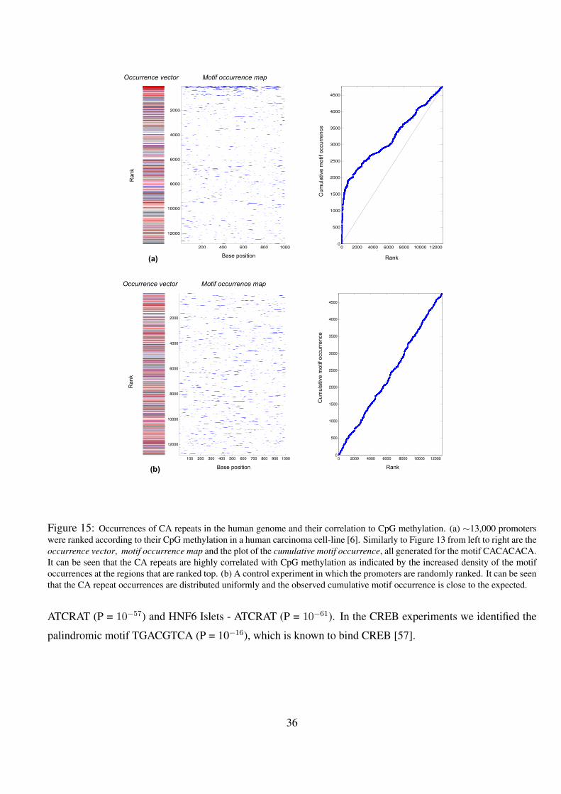
200 400 600 800 1000
2000
4000
6000
8000
10000
12000
Motif map
Base position
Occurence vector
0 2000 4000 6000 8000 10000 120000
500
1000
1500
2000
2500
3000
3500
4000
4500
Sequence rank
Com
ula
tive m
otif occure
nce
100 200 300 400 500 600 700 800 900 1000
2000
4000
6000
8000
10000
12000
Motif map
Base position
Occurence vector
0 2000 4000 6000 8000 10000 120000
500
1000
1500
2000
2500
3000
3500
4000
4500
Sequence rank
Com
ula
tive m
otif
occure
nce
Motif occurrence mapOccurrence vector
Base position
Cumulative motif occurrence
Rank
Motif occurrence mapOccurrence vector
Base position
Cumulative motif occurrence
Rank
(a)
(b) Rank
Rank
Figure 15: Occurrences of CA repeats in the human genome and their correlation to CpG methylation. (a) ∼13,000 promoterswere ranked according to their CpG methylation in a human carcinoma cell-line [6]. Similarly to Figure 13 from left to right are theoccurrence vector, motif occurrence map and the plot of the cumulative motif occurrence, all generated for the motif CACACACA.It can be seen that the CA repeats are highly correlated with CpG methylation as indicated by the increased density of the motifoccurrences at the regions that are ranked top. (b) A control experiment in which the promoters are randomly ranked. It can be seenthat the CA repeat occurrences are distributed uniformly and the observed cumulative motif occurrence is close to the expected.
ATCRAT (P = 10−57) and HNF6 Islets - ATCRAT (P = 10−61). In the CREB experiments we identified the
palindromic motif TGACGTCA (P = 10−16), which is known to bind CREB [57].
36
5.5 Comparison to other methods
Three properties of the mHG enrichment score embodied in DRIM offer advantages over other motif discov-
ery methods: the dynamic cutoff; the rigorous control over false positives and the motif multiplicity model.
5.5.1 Dynamic vs. rigid cutoffs
Most methods use an arbitrary cutoff for set partition. For example, in previous work [1] the authors use
a cutoff of p-value<10−3 on the ChIP-chip signal in order to define the target set for motif searching. In
contrast, the mHG score uses a data driven flexible cutoff and chooses the set partition that maximizes the
motif enrichment.
To more systematically investigate the advantages of using a flexible cutoff we compared mHG with
fixed set partition HG [16] by disabling the flexible cutoff feature in DRIM. The comparison was performed
on ChIP-chip data of TFs whose motif binding sites are well characterized as well as on the Aro80 novel
binding site (described in Section 5.2.1). For each TF we ranked the sequences according to the ChIP-chip
binding signal, generated the motif occurrence vector and computed its HG enrichment using fixed target
sets containing the top 10, 100, 1000 sequences as well as all sequences with ChiP-chip signal < 10−3. The
results are summarized in Figure 16. We note that all of the scores are corrected for multiple motif testing.
The mHG score is also corrected for the multiple cutoff testing. The mHG method yields superior results in
all 6 cases.
We performed additional comparisons of the mHG versus the HG methods by applying both methods to
simulations of motif occurrence vectors (see Section 7.3). In these simulations mHG showed significantly
better performance than HG.
To further investigate the issue of setting a cutoff we compare, for a given TF and condition in the ChIP-
chip dataset, the number of promoters for which the binding signal < 10−3 (denoted #(10−3)) with the
number of promoters at which mHG was attained (denoted n∗). For 82 experiments #(10−3) ≤ 4 and for
46 of these #(10−3) = 0. In these cases a 10−3 fixed cutoff reduces the size of the target set and limits the
usability of the any discovery algorithm. In Figure 17 we compare #(10−3) and n∗ for some of the cases
at which a motif was found by mHG. Note that in a significant number of cases the mHG score identified a
significantly enriched motif even when #(10−3) was very low. One extreme case is the TF SOK2 in YPD
condition for which #(10−3) = 0, yet mHG found a significantly enriched motif.
37
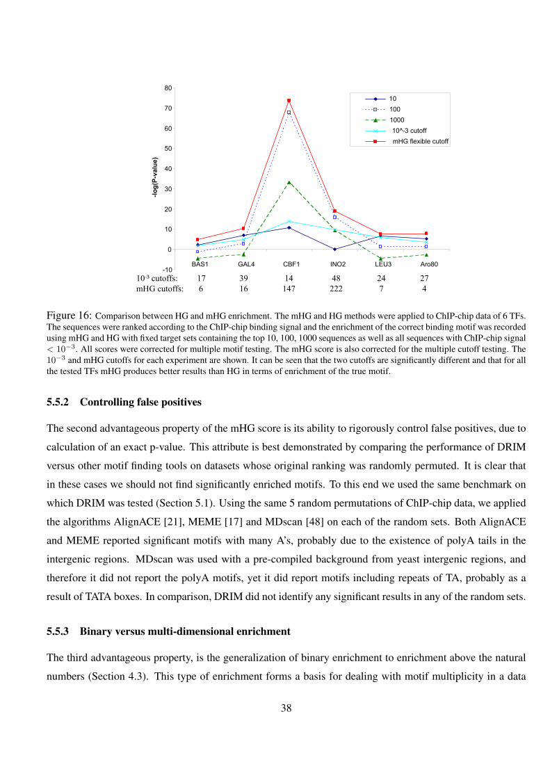
-10
0
10
20
30
40
50
60
70
80
BAS1 GAL4 CBF1 INO2 LEU3 Aro80
-log(P-value)
10
100
1000
10^-3 cutoff
mHG flexible cutoff
10-3 cutoffs: 17 39 14 48 24 27
mHG cutoffs: 6 16 147 222 7 4
Figure 16: Comparison between HG and mHG enrichment. The mHG and HG methods were applied to ChIP-chip data of 6 TFs.The sequences were ranked according to the ChIP-chip binding signal and the enrichment of the correct binding motif was recordedusing mHG and HG with fixed target sets containing the top 10, 100, 1000 sequences as well as all sequences with ChIP-chip signal< 10−3. All scores were corrected for multiple motif testing. The mHG score is also corrected for the multiple cutoff testing. The10−3 and mHG cutoffs for each experiment are shown. It can be seen that the two cutoffs are significantly different and that for allthe tested TFs mHG produces better results than HG in terms of enrichment of the true motif.
5.5.2 Controlling false positives
The second advantageous property of the mHG score is its ability to rigorously control false positives, due to
calculation of an exact p-value. This attribute is best demonstrated by comparing the performance of DRIM
versus other motif finding tools on datasets whose original ranking was randomly permuted. It is clear that
in these cases we should not find significantly enriched motifs. To this end we used the same benchmark on
which DRIM was tested (Section 5.1). Using the same 5 random permutations of ChIP-chip data, we applied
the algorithms AlignACE [21], MEME [17] and MDscan [48] on each of the random sets. Both AlignACE
and MEME reported significant motifs with many A’s, probably due to the existence of polyA tails in the
intergenic regions. MDscan was used with a pre-compiled background from yeast intergenic regions, and
therefore it did not report the polyA motifs, yet it did report motifs including repeats of TA, probably as a
result of TATA boxes. In comparison, DRIM did not identify any significant results in any of the random sets.
5.5.3 Binary versus multi-dimensional enrichment
The third advantageous property, is the generalization of binary enrichment to enrichment above the natural
numbers (Section 4.3). This type of enrichment forms a basis for dealing with motif multiplicity in a data
38
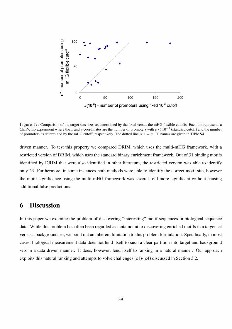
0
50
100
0 50 100 150 200
#(10-3
) - number of promoters using fixed 10-3
cutoff
n*
- num
ber
of pro
mote
rs u
sin
g
mH
G fle
xib
le c
uto
ff
Figure 17: Comparison of the target sets sizes as determined by the fixed versus the mHG flexible cutoffs. Each dot represents aChIP-chip experiment where the x and y coordinates are the number of promoters with p < 10−3 (standard cutoff) and the numberof promoters as determined by the mHG cutoff, respectively. The dotted line is x = y. TF names are given in Table S4
driven manner. To test this property we compared DRIM, which uses the multi-mHG framework, with a
restricted version of DRIM, which uses the standard binary enrichment framework. Out of 31 binding motifs
identified by DRIM that were also identified in other literature, the restricted version was able to identify
only 23. Furthermore, in some instances both methods were able to identify the correct motif site, however
the motif significance using the multi-mHG framework was several fold more significant without causing
additional false predictions.
6 Discussion
In this paper we examine the problem of discovering “interesting” motif sequences in biological sequence
data. While this problem has often been regarded as tantamount to discovering enriched motifs in a target set
versus a background set, we point out an inherent limitation to this problem formulation. Specifically, in most
cases, biological measurement data does not lend itself to such a clear partition into target and background
sets in a data driven manner. It does, however, lend itself to ranking in a natural manner. Our approach
exploits this natural ranking and attempts to solve challenges (c1)-(c4) discussed in Section 3.2.
39
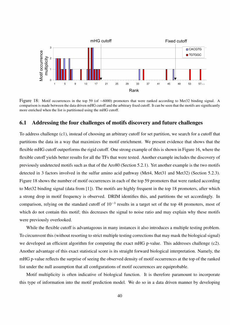
0
1
2
3
1 5 9 13 17 21 25 29 33 37 41 45 49 53 57
CACGTG
TGTGGC
Rank
Motif occurrence
multiplicity
mHG cutoff
...
Fixed cutoff
Figure 18: Motif occurrences in the top 59 (of ∼6000) promoters that were ranked according to Met32 binding signal. Acomparison is made between the data driven mHG cutoff and the arbitrary fixed cutoff. It can be seen that the motifs are significantlymore enriched when the list is partitioned using the mHG cutoff.
6.1 Addressing the four challenges of motifs discovery and future challenges
To address challenge (c1), instead of choosing an arbitrary cutoff for set partition, we search for a cutoff that
partitions the data in a way that maximizes the motif enrichment. We present evidence that shows that the
flexible mHG cutoff outperforms the rigid cutoff. One strong example of this is shown in Figure 16, where the
flexible cutoff yields better results for all the TFs that were tested. Another example includes the discovery of
previously undetected motifs such as that of the Aro80 (Section 5.2.1). Yet another example is the two motifs
detected in 3 factors involved in the sulfur amino acid pathway (Met4, Met31 and Met32) (Section 5.2.3).
Figure 18 shows the number of motif occurrences in each of the top 59 promoters that were ranked according
to Met32 binding signal (data from [1]). The motifs are highly frequent in the top 18 promoters, after which
a strong drop in motif frequency is observed. DRIM identifies this, and partitions the set accordingly. In
comparison, relying on the standard cutoff of 10−3 results in a target set of the top 48 promoters, most of
which do not contain this motif; this decreases the signal to noise ratio and may explain why these motifs
were previously overlooked.
While the flexible cutoff is advantageous in many instances it also introduces a multiple testing problem.
To circumvent this (without resorting to strict multiple testing corrections that may mask the biological signal)
we developed an efficient algorithm for computing the exact mHG p-value. This addresses challenge (c2).
Another advantage of this exact statistical score is its straight forward biological interpretation. Namely, the
mHG p-value reflects the surprise of seeing the observed density of motif occurrences at the top of the ranked
list under the null assumption that all configurations of motif occurrences are equiprobable.
Motif multiplicity is often indicative of biological function. It is therefore paramount to incorporate
this type of information into the motif prediction model. We do so in a data driven manner by developing
40

the multi-mHG framework described in Section 4.3, thus addressing challenge (c3). The advantages of the
multi-mHG model over the binary model are presented in Section 5.5, where the multi-mHG was able to
identify true motifs that elude the binary model.
False prediction of motifs in randomly generated data is often mentioned as one of the drawbacks of
computational motif discovery [1]. In Section 5.1 we report testing DRIM on random permutations of ranked
sequences. When tested on more than 400,000 motifs, DRIM did not report any significant motifs, thus
addressing challenge (c4). The same benchmark was applied to other methods (Section 5.5). All of the
methods reported motifs with significant scores when applied to random sets of sequences. The low false
positive prediction of our method is mainly attributed to the fact that it is based on rigorous statistics and
relies on an exact p-value.
Another important issue that still requires consideration is the characterization of the motif search space.
In this study we performed an exhaustive scanning of a restricted motif space (containing ∼ 105 motifs)
followed by a heuristic search for larger motifs (see Section 4.5). However, the motif search space can be
further extended to include motifs that are longer, “fuzzier” or more complex. Additional considerations
such as the distance of the motif from the transcription start site may be taken into account as well as logical
relations between different motifs (e.g. ’OR’, ’AND’ operations). It is clear that many of these features are
required to correctly model complex regulation patterns that are observed in higher eukaryotes. However,
Two inherent limitations need to be considered when extending the search space: First, as the size of the
motif search space increases the problem of efficiently searching the defined space becomes more acute in
terms of running time. Second, since the size of the search space is virtually endless, the problem of multiple
testing rapidly erodes the signal to noise ratio, requiring an appropriate refinement of the statistical models.
6.2 Sequence length bias in ChIP-chip data
A dataset containing the ChIP-chip data of all 203 putative TFs in Saccharomyces cerevisiae [1, 42] was
constructed. Surprisingly we found that roughly third of these experiments had significantly longer sequences
at the top of the ranked list, which means that for some TFs, longer sequences tend to get stronger TF binding
signals. This observation is unexpected since, although longer probes hybridize more labeled material than
shorter probes the increase is proportional in both channels. It might be caused by some bias in the ChIP-chip
protocol. Alternatively, non-specific bindings between TFs and DNA may explain why longer sequences
bind more TFs. This explanation is also consistent with the “TF sliding hypothesis” [58]. Why only some
TFs exhibit this length bias binding tendency while others don’t remains an open question. We note that this
phenomenon may cause spurious results under our model assumptions and hence we filtered out all ChIP-chip
experiments that had length bias.
41
6.3 Novel motifs in ChIP-chip data
We analyzed the ChIP-chip datasets using DRIM and identified 50 novel putative TFBS motifs that were
previously undetected using 6 other computational methods run on the same data [1]. Next, we turned to
assess whether these motifs have a biological function or, alternatively, they are a result of some bias in
the data or statistical model. We found that 7 of these putative motifs have been previously identified using
techniques other than ChIP-chip. Furthermore, 10 match conserved regulatory sites in yeast that were recently
reported [45]. Taken together this is a strong indication that many of the new motifs DRIM is picking up on
are true biological signals. We then turned to further analyze some of these motifs.
One interesting finding is that the Aro80 motif we identified, which exists only in 7 copies throughout
the entire yeast genome, resides in Aro80’s own promoter. This seems to suggest that Aro80 regulates its
own transcription by binding to its own promoter. We also present a experimentally testable hypothesis to the
regulation of the Aro80 pathway in Section 7.4.
Another interesting observation are the CA repeat motifs, which we identified in 7 different yeast TFs as
well as in human DNA methylation. This type of low complexity motifs have so far been mostly ignored or
filtered out by other computational methods. By contrast there is no need to resolve to this type of artificial
filtering when using the mHG statistics. Our findings in yeast suggest that for certain TFs there is a significant
correlation between a sequence’s capacity to bind a TF and the presence of a CA repeat in the sequence. This
supports a previous hypothesis that CA repeats alter the structure of DNA and thus contribute to TF binding
[49]. Our findings constitute concrete examples of this phenomenon and suggest it may be more frequent
than previously thought.
6.4 Novel motifs in CpG data
We also applied DRIM to high-throughput measurements of methylated CpG islands [6] in human cancer
cells, in order to try and identify motifs that are enriched in hyper methylated regions. Interestingly, we
identified GA and CA repeat elements as highly enriched in methylated CpG regions of 4 different cancer
cell-lines. This is in agreement with previous studies of CpG methylated regions in other cell-lines [52, 53].
It is interesting to ask whether these repeat elements play some active role in the CpG methylation. In [53] the
authors give statistical argumentation against such a hypothesis. Instead, they hypothesize that CA (or TG)
repeats are caused by an increased mutation rate of methylated CpGs that are deaminated into TpGs. Even
if true, this still does not explain the enrichment of the GA repeats. Further experimental and bioinformatics
interrogation of this point is therefore called upon.
Overall, DRIM discovered 10 novel motifs in methylated CpG regions. Strikingly, 9 of them are similar
42
to DNA sequence elements that bind the Polycomb complex in drosophila and/or human [8, 9, 10]. The
Polycomb complex is involved in epigenetic silencing via histone methylation. The suggested link between
histone methylation and CpG methylation is in agreement with recent work that demonstrated the EZH2
protein interacts with DNA methyltransferases via the Polycomb complex [55]. We also note that the DNA
sequence motifs of the two pathways were conserved in drosophila and human, which is complement to the
observation that the Polycomb proteins are evolutionary conserved [59, 10]. Another interesting observation
is that many of the motifs we found in the CpG methylated data are similar across different types of cancer-
cells. This may suggest that the CpG methylation mechanism is orchestrated by DNA binding factors that
are similar in different types of cancer-cells.
6.5 Concluding remarks
Perhaps the most important conclusion that can be drawn from this study is that looking at biological sequence
data in a ranked manner rather than using an arbitrary fixed cutoff to partition the data enables the detection
of biological signals that are otherwise overlooked. This suggests that other motif detection methods that
rely on fixed cutoffs may benefit from dynamic partitioning. While the effectiveness of our approach was
demonstrated mainly on ChIP-chip and methylation data it can also be applied to a wide range of other data
types such as expression data or GO analysis (for details see Section 7.5). The DRIM application is publicly
available at: http://bioinfo.cs.technion.ac.il/drim.
References[1] C.T. Harbison, D.B. Gordon, T.I. Lee, N.J. Rinaldi, K.D. Macisaac, T.W. Danford, N.M. Hannett, J.B. Tagne, D.B. Reynolds,
J. Yoo, E.G. Jennings, J. Zeitlinger, D.K. Pokholok, M. Kellis, P.A. Rolfe, K.T. Takusagawa, E.S. Lander, D.K. Gifford,
E. Fraenkel, and R.A. Young. Transcriptional regulatory code of a eukaryotic genome. Nature, 431(17004):99–104, 2004.
[2] J. Gorodkin, L. J. Heyer, S. Brunak, and G. D. Stormo. Displaying the information contents of structural RNA alignments:
the structure logos. Computer Applications in Biosciences, 13:583–586, 1997.
[3] I. Iraqui, S. Vissers, B. Andre, and A. Urrestarazu. Transcriptional induction by aromatic amino acids in Saccharomyces
cerevisiae. Molecular Cell Biology, 19:3360–3371, 1999.
[4] PL. Blaiseau and D. Thomas. Multiple transcriptional activation complexes tether the yeast activator Met4 to DNA. EMBO,
17:6327–6336, 1998.
[5] PL. Blaiseau, AD. Isnard, Y. Surdin-Kerjan, and D. Thomas. Met31p and Met32p, two related zinc finger proteins, are
involved in transcriptional regulation of yeast sulfur amino acid metabolism. Molecular Cell Biology, 17:3640–3648, 1997.
43
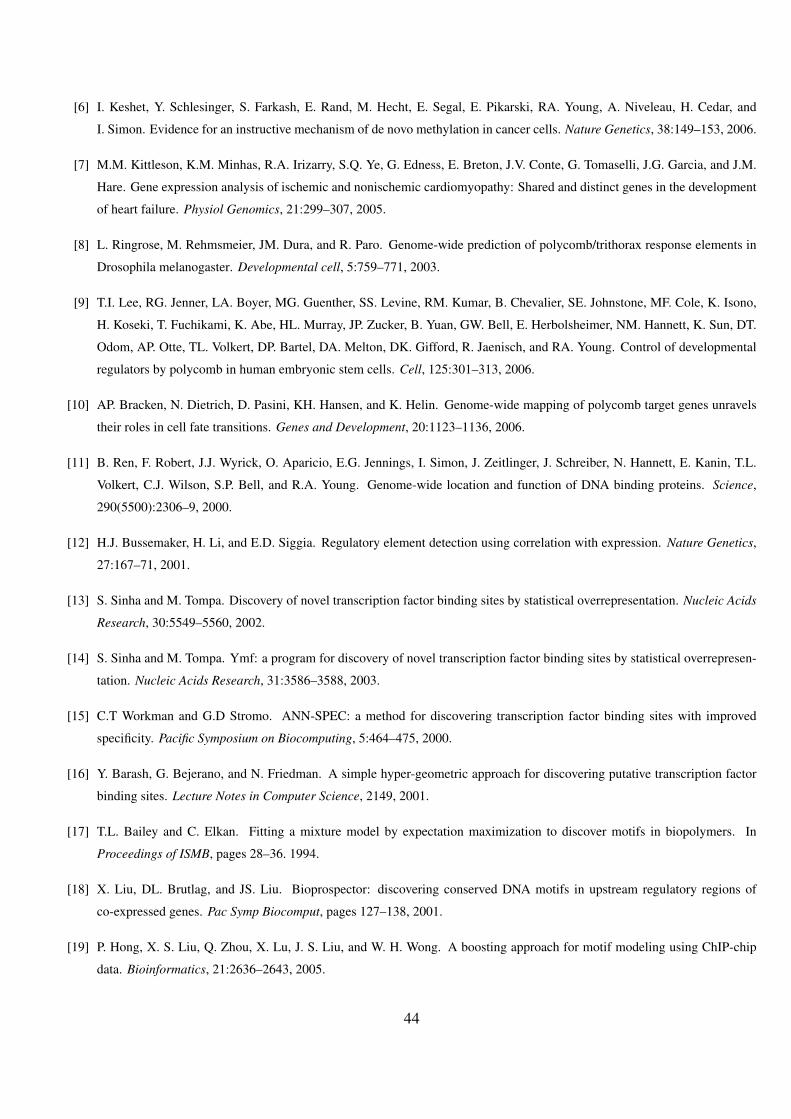
[6] I. Keshet, Y. Schlesinger, S. Farkash, E. Rand, M. Hecht, E. Segal, E. Pikarski, RA. Young, A. Niveleau, H. Cedar, and
I. Simon. Evidence for an instructive mechanism of de novo methylation in cancer cells. Nature Genetics, 38:149–153, 2006.
[7] M.M. Kittleson, K.M. Minhas, R.A. Irizarry, S.Q. Ye, G. Edness, E. Breton, J.V. Conte, G. Tomaselli, J.G. Garcia, and J.M.
Hare. Gene expression analysis of ischemic and nonischemic cardiomyopathy: Shared and distinct genes in the development
of heart failure. Physiol Genomics, 21:299–307, 2005.
[8] L. Ringrose, M. Rehmsmeier, JM. Dura, and R. Paro. Genome-wide prediction of polycomb/trithorax response elements in
Drosophila melanogaster. Developmental cell, 5:759–771, 2003.
[9] T.I. Lee, RG. Jenner, LA. Boyer, MG. Guenther, SS. Levine, RM. Kumar, B. Chevalier, SE. Johnstone, MF. Cole, K. Isono,
H. Koseki, T. Fuchikami, K. Abe, HL. Murray, JP. Zucker, B. Yuan, GW. Bell, E. Herbolsheimer, NM. Hannett, K. Sun, DT.
Odom, AP. Otte, TL. Volkert, DP. Bartel, DA. Melton, DK. Gifford, R. Jaenisch, and RA. Young. Control of developmental
regulators by polycomb in human embryonic stem cells. Cell, 125:301–313, 2006.
[10] AP. Bracken, N. Dietrich, D. Pasini, KH. Hansen, and K. Helin. Genome-wide mapping of polycomb target genes unravels
their roles in cell fate transitions. Genes and Development, 20:1123–1136, 2006.
[11] B. Ren, F. Robert, J.J. Wyrick, O. Aparicio, E.G. Jennings, I. Simon, J. Zeitlinger, J. Schreiber, N. Hannett, E. Kanin, T.L.
Volkert, C.J. Wilson, S.P. Bell, and R.A. Young. Genome-wide location and function of DNA binding proteins. Science,
290(5500):2306–9, 2000.
[12] H.J. Bussemaker, H. Li, and E.D. Siggia. Regulatory element detection using correlation with expression. Nature Genetics,
27:167–71, 2001.
[13] S. Sinha and M. Tompa. Discovery of novel transcription factor binding sites by statistical overrepresentation. Nucleic Acids
Research, 30:5549–5560, 2002.
[14] S. Sinha and M. Tompa. Ymf: a program for discovery of novel transcription factor binding sites by statistical overrepresen-
tation. Nucleic Acids Research, 31:3586–3588, 2003.
[15] C.T Workman and G.D Stromo. ANN-SPEC: a method for discovering transcription factor binding sites with improved
specificity. Pacific Symposium on Biocomputing, 5:464–475, 2000.
[16] Y. Barash, G. Bejerano, and N. Friedman. A simple hyper-geometric approach for discovering putative transcription factor
binding sites. Lecture Notes in Computer Science, 2149, 2001.
[17] T.L. Bailey and C. Elkan. Fitting a mixture model by expectation maximization to discover motifs in biopolymers. In
Proceedings of ISMB, pages 28–36. 1994.
[18] X. Liu, DL. Brutlag, and JS. Liu. Bioprospector: discovering conserved DNA motifs in upstream regulatory regions of
co-expressed genes. Pac Symp Biocomput, pages 127–138, 2001.
[19] P. Hong, X. S. Liu, Q. Zhou, X. Lu, J. S. Liu, and W. H. Wong. A boosting approach for motif modeling using ChIP-chip
data. Bioinformatics, 21:2636–2643, 2005.
44
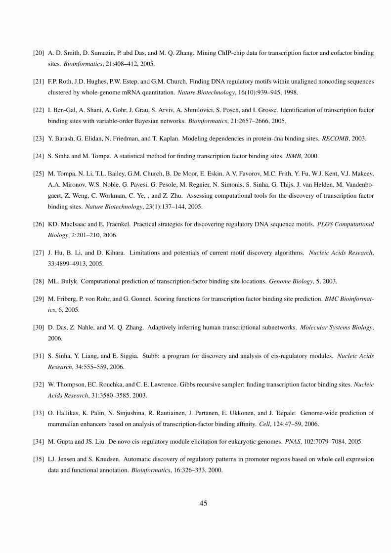
[20] A. D. Smith, D. Sumazin, P. abd Das, and M. Q. Zhang. Mining ChIP-chip data for transcription factor and cofactor binding
sites. Bioinformatics, 21:408–412, 2005.
[21] F.P. Roth, J.D. Hughes, P.W. Estep, and G.M. Church. Finding DNA regulatory motifs within unaligned noncoding sequences
clustered by whole-genome mRNA quantitation. Nature Biotechnology, 16(10):939–945, 1998.
[22] I. Ben-Gal, A. Shani, A. Gohr, J. Grau, S. Arviv, A. Shmilovici, S. Posch, and I. Grosse. Identification of transcription factor
binding sites with variable-order Bayesian networks. Bioinformatics, 21:2657–2666, 2005.
[23] Y. Barash, G. Elidan, N. Friedman, and T. Kaplan. Modeling dependencies in protein-dna binding sites. RECOMB, 2003.
[24] S. Sinha and M. Tompa. A statistical method for finding transcription factor binding sites. ISMB, 2000.
[25] M. Tompa, N. Li, T.L. Bailey, G.M. Church, B. De Moor, E. Eskin, A.V. Favorov, M.C. Frith, Y. Fu, W.J. Kent, V.J. Makeev,
A.A. Mironov, W.S. Noble, G. Pavesi, G. Pesole, M. Regnier, N. Simonis, S. Sinha, G. Thijs, J. van Helden, M. Vandenbo-
gaert, Z. Weng, C. Workman, C. Ye, , and Z. Zhu. Assessing computational tools for the discovery of transcription factor
binding sites. Nature Biotechnology, 23(1):137–144, 2005.
[26] KD. MacIsaac and E. Fraenkel. Practical strategies for discovering regulatory DNA sequence motifs. PLOS Computational
Biology, 2:201–210, 2006.
[27] J. Hu, B. Li, and D. Kihara. Limitations and potentials of current motif discovery algorithms. Nucleic Acids Research,
33:4899–4913, 2005.
[28] ML. Bulyk. Computational prediction of transcription-factor binding site locations. Genome Biology, 5, 2003.
[29] M. Friberg, P. von Rohr, and G. Gonnet. Scoring functions for transcription factor binding site prediction. BMC Bioinformat-
ics, 6, 2005.
[30] D. Das, Z. Nahle, and M. Q. Zhang. Adaptively inferring human transcriptional subnetworks. Molecular Systems Biology,
2006.
[31] S. Sinha, Y. Liang, and E. Siggia. Stubb: a program for discovery and analysis of cis-regulatory modules. Nucleic Acids
Research, 34:555–559, 2006.
[32] W. Thompson, EC. Rouchka, and C. E. Lawrence. Gibbs recursive sampler: finding transcription factor binding sites. Nucleic
Acids Research, 31:3580–3585, 2003.
[33] O. Hallikas, K. Palin, N. Sinjushina, R. Rautiainen, J. Partanen, E. Ukkonen, and J. Taipale. Genome-wide prediction of
mammalian enhancers based on analysis of transcription-factor binding affinity. Cell, 124:47–59, 2006.
[34] M. Gupta and JS. Liu. De novo cis-regulatory module elicitation for eukaryotic genomes. PNAS, 102:7079–7084, 2005.
[35] LJ. Jensen and S. Knudsen. Automatic discovery of regulatory patterns in promoter regions based on whole cell expression
data and functional annotation. Bioinformatics, 16:326–333, 2000.
45
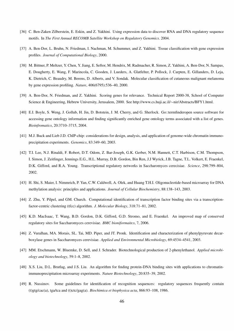
[36] C. Ben-Zaken Zilberstein, E. Eskin, and Z. Yakhini. Using expression data to discover RNA and DNA regulatory sequence
motifs. In The First Annual RECOMB Satellite Workshop on Regulatory Genomics. 2004.
[37] A. Ben-Dor, L. Bruhn, N. Friedman, I. Nachman, M. Schummer, and Z. Yakhini. Tissue classification with gene expression
profiles. Journal of Computational Biology, 2000.
[38] M. Bittner, P. Meltzer, Y. Chen, Y. Jiang, E. Seftor, M. Hendrix, M. Radmacher, R. Simon, Z. Yakhini, A. Ben-Dor, N. Sampas,
E. Dougherty, E. Wang, F. Marincola, C. Gooden, J. Lueders, A. Glatfelter, P. Pollock, J. Carpten, E. Gillanders, D. Leja,
K. Dietrich, C. Beaudry, M. Berens, D. Alberts, and V. Sondak. Molecular classification of cutaneous malignant melanoma
by gene expression profiling. Nature, 406(6795):536–40, 2000.
[39] A. Ben-Dor, N. Friedman, and Z. Yakhini. Scoring genes for relevance. Technical Report 2000-38, School of Computer
Science & Engineering, Hebrew University, Jerusalem, 2000. See http://www.cs.huji.ac.il/∼nir/Abstracts/BFY1.html.
[40] E.I. Boyle, S. Weng, J. Gollub, H. Jin, D. Botstein, J. M. Cherry, and G. Sherlock. Go::termfinderopen source software for
accessing gene ontology information and finding significantly enriched gene ontology terms associated with a list of genes.
Bioinfromatics, 20:3710–3715, 2004.
[41] M.J. Buck and Lieb J.D. ChIP-chip: considerations for design, analysis, and application of genome-wide chromatin immuno-
precipitation experiments. Genomics, 83:349–60, 2003.
[42] T.I. Lee, N.J. Rinaldi, F. Robert, D.T. Odom, Z. Bar-Joseph, G.K. Gerber, N.M. Hannett, C.T. Harbison, C.M. Thompson,
I. Simon, J. Zeitlinger, Jennings E.G., H.L. Murray, D.B. Gordon, Bin Ren, J.J Wyrick, J.B. Tagne, T.L. Volkert, E. Fraenkel,
D.K. Gifford, and R.A. Young. Transcriptional regulatory networks in Saccharomyces cerecisiae. Science, 298:799–804,
2002.
[43] H. Shi, S. Maier, I. Nimmrich, P. Yan, C.W. Caldwell, A. Olek, and Huang T.H.I. Oligonucleotide-based microarray for DNA
methylation analysis: principles and applications. Journal of Cellular Biochemistry, 88:138–143, 2003.
[44] Z. Zhu, Y. Pilpel, and GM. Church. Computational identification of transcription factor binding sites via a transcription-
factor-centric clustering (tfcc) algorithm. J. Molecular Biology, 318:71–81, 2002.
[45] K.D. MacIsaac, T. Wang, B.D. Gordon, D.K. Gifford, G.D. Stromo, and E. Fraenkel. An improved map of conserved
regulatory sites for Saccharomyces cerevisiae. BMC bioniformaitcs, 7, 2006.
[46] Z. Vuralhan, MA. Morais, SL. Tai, MD. Piper, and JT. Pronk. Identification and characterization of phenylpyruvate decar-
boxylase genes in Saccharomyces cerevisiae. Applied and Environmental Microbiology, 69:4534–4541, 2003.
[47] MM. Etschmann, W. Bluemke, D. Sell, and J. Schrader. Biotechnological production of 2-phenylethanol. Applied microbi-
ology and biotechnology, 59:1–8, 2002.
[48] X.S. Liu, D.L. Brutlag, and J.S. Liu. An algorithm for finding protein-DNA binding sites with applications to chromatin-
immunoprecipitation microarray experiments. Nature Biotechnology, 20:835–39, 2002.
[49] R. Nussinov. Some guidelines for identification of recognition sequences: regulatory sequences frequently contain
(t)gtg/cac(a), tga/tca and (t)ctc/gag(a). Biochimica et biophysica acta, 866:93–108, 1986.
46
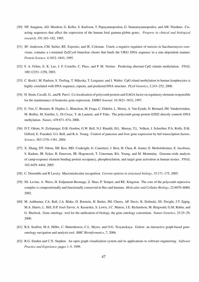
[50] NP. Anagnou, AD. Moulton, G. Keller, S. Karlsson, T. Papayannopoulou, G. Stamatoyannopoulos, and AW. Nienhuis. Cis-
acting sequences that affect the expression of the human fetal gamma-globin genes. Progress in clinical and biological
research, 191:163–182, 1985.
[51] SF. Anderson, CM. Steber, RE. Esposito, and JE. Coleman. Ume6, a negative regulator of meiosis in Saccharomyces cere-
visiae, contains a c-terminal Zn2Cys6 binuclear cluster that binds the URS1 DNA sequence in a zinc-dependent manner.
Protein Science, 4:1832–1843, 1995.
[52] F. A. Feltus, E. K. Lee, J. F. Costello, C. Plass, and P. M. Vertino. Predicting aberrant CpG islands methylation. PNAS,
100:12253–1258, 2003.
[53] C. Bock1, M. Paulsen, S. Tierling, T. Mikeska, T. Lengauer, and J. Walter. CpG island methylation in human lymphocytes is
highly correlated with DNA sequence, repeats, and predicted DNA structure. PLoS Genetics, 2:243–252, 2006.
[54] H. Strutt, Cavalli. G., and R. Paro1. Co-localization of polycomb protein and GAGA factor on regulatory elements responsible
for the maintenance of homeotic gene expression. EMBO Journal, 16:3621–3632, 1997.
[55] E. Vire, C. Brenner, R. Deplus, L. Blanchon, M. Fraga, C. Didelot, L. Morey, A. Van Eynde, D. Bernard, JM. Vanderwinden,
M. Bollen, M. Esteller, L. Di Croce, Y. de Launoit, and F Fuks. The polycomb group protein EZH2 directly controls DNA
methylation. Nature, 439:871–874, 2006.
[56] D.T. Odom, N. Zizlsperger, D.B. Gordon, G.W. Bell, N.J. Rinaldi, H.L. Murray, T.L. Volkert, J. Schreiber, P.A. Rolfe, D.K.
Gifford, E. Fraenkel, G.I. Bell, and R.A. Young. Control of pancreas and liver gene expression by hnf transcription factors.
Science, 303:1378–1381, 2004.
[57] X. Zhang, DT. Odom, SH. Koo, MD. Conkright, G. Canettieri, J. Best, H. Chen, R. Jenner, E. Herbolsheimer, E. Jacobsen,
S. Kadam, JR. Ecker, B. Emerson, JB. Hogenesch, T. Unterman, RA. Young, and M. Montminy. Genome-wide analysis
of camp-response element binding protein occupancy, phosphorylation, and target gene activation in human tissues. PNAS,
102:4459–4464, 2005.
[58] C. Deremble and R Lavery. Macromolecular recognition. Current opinion in structural biology, 15:171–175, 2005.
[59] SS. Levine, A. Weiss, H. Erdjument-Bromage, Z. Shao, P. Tempst, and RE. Kingston. The core of the polycomb repressive
complex is compositionally and functionally conserved in flies and humans. Molecular and Cellular Biology, 22:6070–6080,
2002.
[60] M. Ashburner, CA. Ball, J.A. Blake, D. Botstein, H. Butler, JM. Cherry, AP. Davis, K. Dolinski, SS. Dwight, J.T. Eppig,
M.A. Harris, L. Hill, D.P. Issel-Tarver, A. Kasarskis, S. Lewis, J.C. Matese, J.E. Richardson, M. Ringwald, G.M. Rubin, and
G. Sherlock. Gene ontology: tool for the unification of biology. the gene ontology consortium. Nature Genetics, 25:25–29,
2000.
[61] R.S. Sealfon, M.A. Hibbs, C. Huttenhower, C.L. Myers, and O.G. Troyanskaya. Golem: an interactive graph-based gene-
ontology navigation and analysis tool. BMC Bioinformatics, 7, 2006.
[62] R.G. Emden and C.N. Stephen. An open graph visualization system and its applications to software engineering. Software
Practice and Expirience, pages 1–5, 1999.
47

7 Appendix I - Supplementary material
7.1 Bounds for the mHG p-value
We demonstrate several bounds for pVal(p). These bounds may be used for rapid assessment of the p-value of
a given mHG score, which can be instrumental in improving algorithmic efficiency. In Figure S1 we compare
the bounds with exact p-values as well as with observed frequencies, on randomly generated test cases.
For fixed values of N and B we define HGTn(λ) = HGT(bn(λ); N, B, n). HGT(x; N, B, n) is the
complement of the cumulative distribution function of a hypergeometric random variable. As such, for any
value p we have Prob(HGTn(λ) ≤ p) ≤ p 1. Set an attainable mHG score p. If mHG(λ) = p then there is
some rank n∗ at which this score was attained. Clearly λ : HGTn(λ) ≤ p ⊆ λ : mHG(λ)p. For similar
reasons λ : mHG(λ) ≤ p =⋃N
n=1 λ : HGTn(λ) ≤ p. This leads to the following (trivial) bounds for any
HGTn(λ) attainable p:
p ≤ Prob(mHG(λ) ≤ p) ≤ Np. 2 (18)
In many cases the upper bound provided in (18) is very loose. When B << N the following tighter upper
bound is of greater use (see Figure S1). Fix N and B, and consider the space of all binary label vectors with
B 1’s and N −B 0’s: Λ = 0, 1(N−B,B), endowed with a uniform probability measure.
Theorem 7.1 For any HGTn(λ) attainable p:
p ≤ Prob(mHG(λ) ≤ p) ≤ Bp. (19)
Proof: Note that we only need to test B thresholds to compute mHG(λ). A union bound may therefore
seem applicable. However, since the thresholds depend on the point λ and may be different for different λs
we need to use a more careful argument.
For each 1 ≤ i ≤ B let ni be the maximal rank n for which any vector λ ∈ Λ with bn(λ) ≥ i has a score
HGTn(λ) ≤ p. Formally:
ni = max n : (bn(λ) ≥ i) ⇒ HGTn(λ) ≤ p . (20)
Monotonicity properties of the hypergeometric distribution imply the existence of such numbers ni. By
definition they are constants, independent of λ.
1If X and Z are discrete random variables that take a finite number of values X1 ≤ X2... ≤ Xk and Z1 ≤ Z2... ≤ Zm withprobabilities Ω1 = p1, p2...pk and Ω2 = q1, q2...qm respectively, and P (Z = x) = P (X ≥ x) then the following propertieshold: (1) ∀ p P (Z ≤ p) ≤ p; (2) for any attainable p ∈ Ω2 P (Z ≤ p) = p.
2p = Prob(HGTn(λ) ≤ p) ≤ Prob(mHG(λ) ≤ p) = Prob(⋃N
n=1 λ : HGTn(λ) ≤ p) ≤N∑
n=1Prob(HGTn(λ) ≤ p) ≤ Np.
48
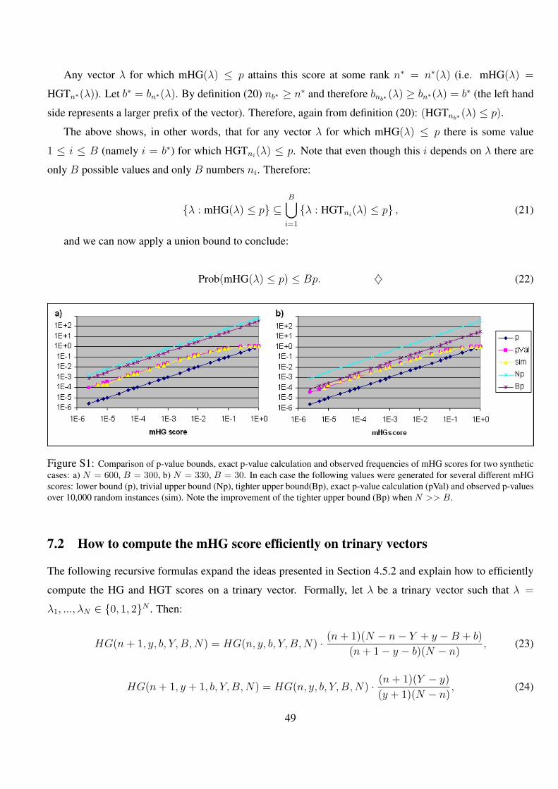
Any vector λ for which mHG(λ) ≤ p attains this score at some rank n∗ = n∗(λ) (i.e. mHG(λ) =
HGTn∗(λ)). Let b∗ = bn∗(λ). By definition (20) nb∗ ≥ n∗ and therefore bnb∗ (λ) ≥ bn∗(λ) = b∗ (the left hand
side represents a larger prefix of the vector). Therefore, again from definition (20): (HGTnb∗ (λ) ≤ p).
The above shows, in other words, that for any vector λ for which mHG(λ) ≤ p there is some value
1 ≤ i ≤ B (namely i = b∗) for which HGTni(λ) ≤ p. Note that even though this i depends on λ there are
only B possible values and only B numbers ni. Therefore:
λ : mHG(λ) ≤ p ⊆B⋃
i=1
λ : HGTni(λ) ≤ p , (21)
and we can now apply a union bound to conclude:
Prob(mHG(λ) ≤ p) ≤ Bp. ♦ (22)
Figure S1: Comparison of p-value bounds, exact p-value calculation and observed frequencies of mHG scores for two syntheticcases: a) N = 600, B = 300, b) N = 330, B = 30. In each case the following values were generated for several different mHGscores: lower bound (p), trivial upper bound (Np), tighter upper bound(Bp), exact p-value calculation (pVal) and observed p-valuesover 10,000 random instances (sim). Note the improvement of the tighter upper bound (Bp) when N >> B.
7.2 How to compute the mHG score efficiently on trinary vectors
The following recursive formulas expand the ideas presented in Section 4.5.2 and explain how to efficiently
compute the HG and HGT scores on a trinary vector. Formally, let λ be a trinary vector such that λ =
λ1, ..., λN ∈ 0, 1, 2N . Then:
HG(n + 1, y, b, Y, B, N) = HG(n, y, b, Y, B,N) · (n + 1)(N − n− Y + y −B + b)
(n + 1− y − b)(N − n), (23)
HG(n + 1, y + 1, b, Y, B, N) = HG(n, y, b, Y, B,N) · (n + 1)(Y − y)
(y + 1)(N − n), (24)
49
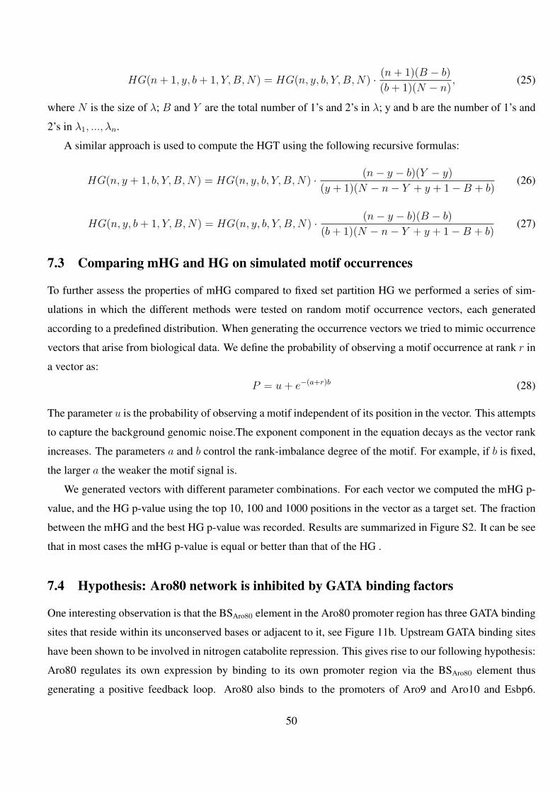
HG(n + 1, y, b + 1, Y, B, N) = HG(n, y, b, Y, B,N) · (n + 1)(B − b)
(b + 1)(N − n), (25)
where N is the size of λ; B and Y are the total number of 1’s and 2’s in λ; y and b are the number of 1’s and
2’s in λ1, ..., λn.
A similar approach is used to compute the HGT using the following recursive formulas:
HG(n, y + 1, b, Y, B, N) = HG(n, y, b, Y, B,N) · (n− y − b)(Y − y)
(y + 1)(N − n− Y + y + 1−B + b)(26)
HG(n, y, b + 1, Y, B, N) = HG(n, y, b, Y, B,N) · (n− y − b)(B − b)
(b + 1)(N − n− Y + y + 1−B + b)(27)
7.3 Comparing mHG and HG on simulated motif occurrences
To further assess the properties of mHG compared to fixed set partition HG we performed a series of sim-
ulations in which the different methods were tested on random motif occurrence vectors, each generated
according to a predefined distribution. When generating the occurrence vectors we tried to mimic occurrence
vectors that arise from biological data. We define the probability of observing a motif occurrence at rank r in
a vector as:
P = u + e−(a+r)b (28)
The parameter u is the probability of observing a motif independent of its position in the vector. This attempts
to capture the background genomic noise.The exponent component in the equation decays as the vector rank
increases. The parameters a and b control the rank-imbalance degree of the motif. For example, if b is fixed,
the larger a the weaker the motif signal is.
We generated vectors with different parameter combinations. For each vector we computed the mHG p-
value, and the HG p-value using the top 10, 100 and 1000 positions in the vector as a target set. The fraction
between the mHG and the best HG p-value was recorded. Results are summarized in Figure S2. It can be see
that in most cases the mHG p-value is equal or better than that of the HG .
7.4 Hypothesis: Aro80 network is inhibited by GATA binding factors
One interesting observation is that the BSAro80 element in the Aro80 promoter region has three GATA binding
sites that reside within its unconserved bases or adjacent to it, see Figure 11b. Upstream GATA binding sites
have been shown to be involved in nitrogen catabolite repression. This gives rise to our following hypothesis:
Aro80 regulates its own expression by binding to its own promoter region via the BSAro80 element thus
generating a positive feedback loop. Aro80 also binds to the promoters of Aro9 and Aro10 and Esbp6.
50
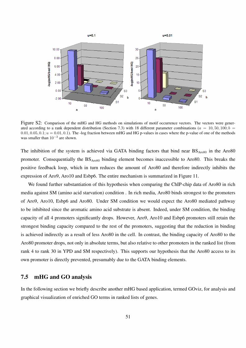
Figure S2: Comparison of the mHG and HG methods on simulations of motif occurrence vectors. The vectors were gener-ated according to a rank dependent distribution (Section 7.3) with 18 different parameter combinations (a = 10, 50, 100; b =0.01, 0.05, 0.1;u = 0.01, 0.1). The -log fraction between mHG and HG p-values in cases where the p-value of one of the methodswas smaller than 10−3 are shown.
The inhibition of the system is achieved via GATA binding factors that bind near BSAro80 in the Aro80
promoter. Consequentially the BSAro80 binding element becomes inaccessible to Aro80. This breaks the
positive feedback loop, which in turn reduces the amount of Aro80 and therefore indirectly inhibits the
expression of Aro9, Aro10 and Esbp6. The entire mechanism is summarized in Figure 11.
We found further substantiation of this hypothesis when comparing the ChIP-chip data of Aro80 in rich
media against SM (amino acid starvation) condition . In rich media, Aro80 binds strongest to the promoters
of Aro9, Aro10, Esbp6 and Aro80. Under SM condition we would expect the Aro80 mediated pathway
to be inhibited since the aromatic amino acid substrate is absent. Indeed, under SM condition, the binding
capacity of all 4 promoters significantly drops. However, Aro9, Aro10 and Esbp6 promoters still retain the
strongest binding capacity compared to the rest of the promoters, suggesting that the reduction in binding
is achieved indirectly as a result of less Aro80 in the cell. In contrast, the binding capacity of Aro80 to the
Aro80 promoter drops, not only in absolute terms, but also relative to other promoters in the ranked list (from
rank 4 to rank 30 in YPD and SM respectively). This supports our hypothesis that the Aro80 access to its
own promoter is directly prevented, presumably due to the GATA binding elements.
7.5 mHG and GO analysis
In the following section we briefly describe another mHG based application, termed GOviz, for analysis and
graphical visualization of enriched GO terms in ranked lists of genes.
51
Recent advances in molecular biology high-throughput technologies (as microarray, ChIP-chip or mDIP)
enable thousands of measurements in a single experiment. Such experiments often produce large lists of
genes that are somehow associated (e.g. a list of genes with similar expression patterns). It is interesting
to try and identify whether there is a common theme or biological phenomenon that links those genes. The
Gene Ontology (GO) Consortium [60] is an ongoing effort aimed at providing controlled vocabularies, which
associate genes with GO terms that fall into 3 categories: Biological Process, Molecular Function and Cel-
lular Component. The GO terms are structured in DAGs (directed acyclic graphs) that capture the relations
and dependencies between the terms [60]. A GO term that is over-represented in the target list of genes may
reveal new insight and common functional characteristics of the genes in the list.
Several excellent tools have been developed for discovering GO terms that are enriched in lists of genes
including [40, 61]. These tools search for enriched GO terms in a target set versus a background set of genes
using the HG model or a binomial approximation of HG [40].
Following the same rational we used for enrichment of sequence motifs, we argue that it is possible
to exploit the inherent ranking property of genomic measurements in order to enhance GO term enrichment
analysis. Instead of using the HG model on fixed sets of genes we developed a GO analysis tool that computes
GO term enrichment in ranked lists of genes using the mHG statistical framework. Two principle issues were
at the focus of the GOviz tool design: (i) ease of usage and (ii) intuitive and easy interpretation of the results.
To enable a straight-forward usage, the GOviz tool has an internal translator, which converts between the user
inputted gene accessions to the accessions used in the GO database in a seeming-less manner. The tool is
highly optimized - ∼10 seconds for running on a list containing ∼10,000 genes on a Pentium IV, 2Ghz, 512
RAM machine. GO analysis tools often return long lists of enriched GO terms, which do not lend themselves
to easy interpretation. We developed a graphical representation of the GO analysis results that attempts to
overcome this issue. The enriched GO terms (with mHG p-value better then a user predefined threshold)
and all their ancestors in the GO DAG are visualized using a colored graph, where the colors of the nodes
reflect the GO term enrichment. An example of the graphical output is shown in Figure S3. The graph is
also clickable and enables easy retrieval of additional information such as genes that are associated with the
enriched GO terms. The tool is implemented in C++ and Perl and invokes Graphviz, an open source graph
visualization software [62]. The tool is publicly available at http://bioinfo.cs.technion.ac.il/GOviz.
52
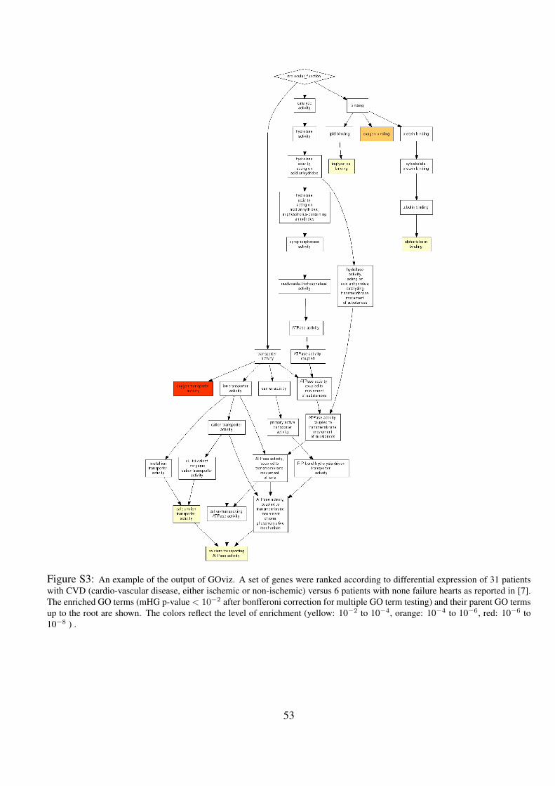
Figure S3: An example of the output of GOviz. A set of genes were ranked according to differential expression of 31 patientswith CVD (cardio-vascular disease, either ischemic or non-ischemic) versus 6 patients with none failure hearts as reported in [7].The enriched GO terms (mHG p-value < 10−2 after bonfferoni correction for multiple GO term testing) and their parent GO termsup to the root are shown. The colors reflect the level of enrichment (yellow: 10−2 to 10−4, orange: 10−4 to 10−6, red: 10−6 to10−8 ) .
53
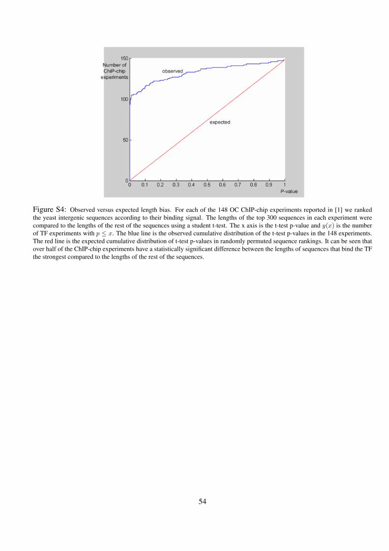
Figure S4: Observed versus expected length bias. For each of the 148 OC ChIP-chip experiments reported in [1] we rankedthe yeast intergenic sequences according to their binding signal. The lengths of the top 300 sequences in each experiment werecompared to the lengths of the rest of the sequences using a student t-test. The x axis is the t-test p-value and y(x) is the numberof TF experiments with p ≤ x. The blue line is the observed cumulative distribution of the t-test p-values in the 148 experiments.The red line is the expected cumulative distribution of t-test p-values in randomly permuted sequence rankings. It can be seen thatover half of the ChIP-chip experiments have a statistically significant difference between the lengths of sequences that bind the TFthe strongest compared to the lengths of the rest of the sequences.
54

Table S1
The list of TFs in the Harbison filtered data set.
55
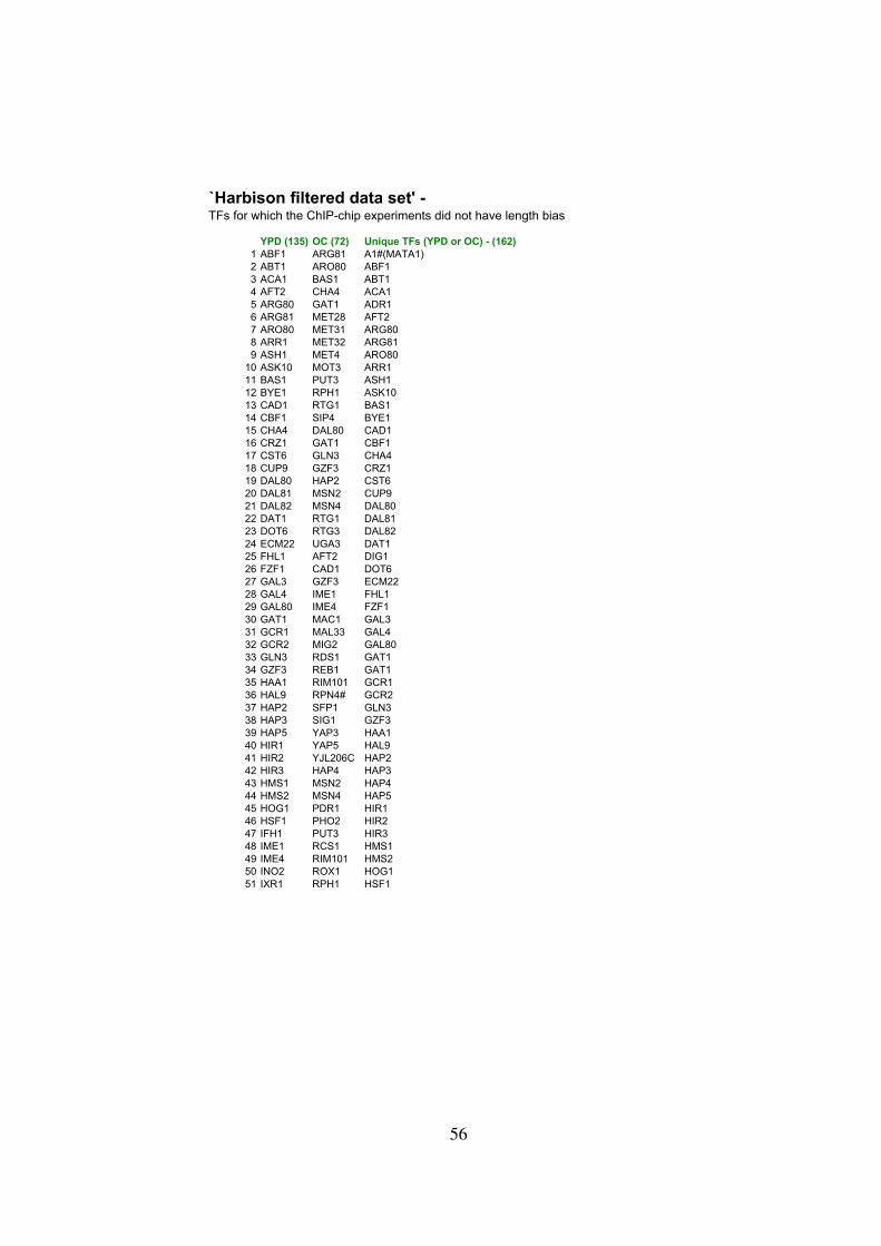
`Harbison filtered data set' - TFs for which the ChIP-chip experiments did not have length bias
YPD (135) OC (72) Unique TFs (YPD or OC) - (162)
1 ABF1 ARG81 A1#(MATA1)
2 ABT1 ARO80 ABF1
3 ACA1 BAS1 ABT1
4 AFT2 CHA4 ACA1
5 ARG80 GAT1 ADR1
6 ARG81 MET28 AFT2
7 ARO80 MET31 ARG80
8 ARR1 MET32 ARG81
9 ASH1 MET4 ARO80
10 ASK10 MOT3 ARR1
11 BAS1 PUT3 ASH1
12 BYE1 RPH1 ASK10
13 CAD1 RTG1 BAS1
14 CBF1 SIP4 BYE1
15 CHA4 DAL80 CAD1
16 CRZ1 GAT1 CBF1
17 CST6 GLN3 CHA4
18 CUP9 GZF3 CRZ1
19 DAL80 HAP2 CST6
20 DAL81 MSN2 CUP9
21 DAL82 MSN4 DAL80
22 DAT1 RTG1 DAL81
23 DOT6 RTG3 DAL82
24 ECM22 UGA3 DAT1
25 FHL1 AFT2 DIG1
26 FZF1 CAD1 DOT6
27 GAL3 GZF3 ECM22
28 GAL4 IME1 FHL1
29 GAL80 IME4 FZF1
30 GAT1 MAC1 GAL3
31 GCR1 MAL33 GAL4
32 GCR2 MIG2 GAL80
33 GLN3 RDS1 GAT1
34 GZF3 REB1 GAT1
35 HAA1 RIM101 GCR1
36 HAL9 RPN4# GCR2
37 HAP2 SFP1 GLN3
38 HAP3 SIG1 GZF3
39 HAP5 YAP3 HAA1
40 HIR1 YAP5 HAL9
41 HIR2 YJL206C HAP2
42 HIR3 HAP4 HAP3
43 HMS1 MSN2 HAP4
44 HMS2 MSN4 HAP5
45 HOG1 PDR1 HIR1
46 HSF1 PHO2 HIR2
47 IFH1 PUT3 HIR3
48 IME1 RCS1 HMS1
49 IME4 RIM101 HMS2
50 INO2 ROX1 HOG1
51 IXR1 RPH1 HSF1
56
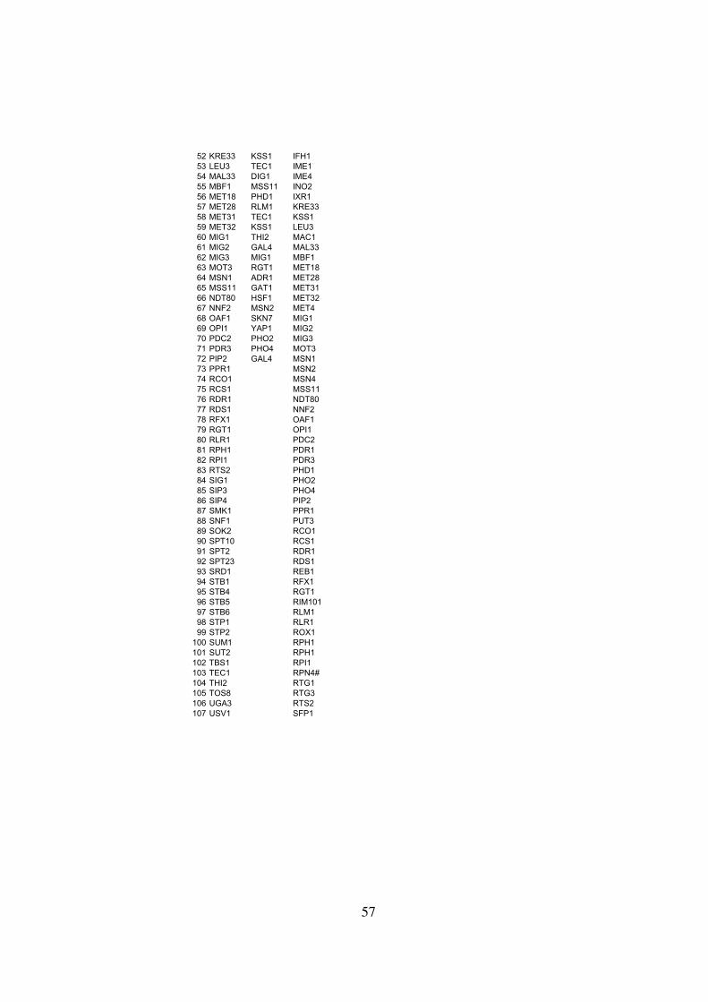
52 KRE33 KSS1 IFH1
53 LEU3 TEC1 IME1
54 MAL33 DIG1 IME4
55 MBF1 MSS11 INO2
56 MET18 PHD1 IXR1
57 MET28 RLM1 KRE33
58 MET31 TEC1 KSS1
59 MET32 KSS1 LEU3
60 MIG1 THI2 MAC1
61 MIG2 GAL4 MAL33
62 MIG3 MIG1 MBF1
63 MOT3 RGT1 MET18
64 MSN1 ADR1 MET28
65 MSS11 GAT1 MET31
66 NDT80 HSF1 MET32
67 NNF2 MSN2 MET4
68 OAF1 SKN7 MIG1
69 OPI1 YAP1 MIG2
70 PDC2 PHO2 MIG3
71 PDR3 PHO4 MOT3
72 PIP2 GAL4 MSN1
73 PPR1 MSN2
74 RCO1 MSN4
75 RCS1 MSS11
76 RDR1 NDT80
77 RDS1 NNF2
78 RFX1 OAF1
79 RGT1 OPI1
80 RLR1 PDC2
81 RPH1 PDR1
82 RPI1 PDR3
83 RTS2 PHD1
84 SIG1 PHO2
85 SIP3 PHO4
86 SIP4 PIP2
87 SMK1 PPR1
88 SNF1 PUT3
89 SOK2 RCO1
90 SPT10 RCS1
91 SPT2 RDR1
92 SPT23 RDS1
93 SRD1 REB1
94 STB1 RFX1
95 STB4 RGT1
96 STB5 RIM101
97 STB6 RLM1
98 STP1 RLR1
99 STP2 ROX1
100 SUM1 RPH1
101 SUT2 RPH1
102 TBS1 RPI1
103 TEC1 RPN4#
104 THI2 RTG1
105 TOS8 RTG3
106 UGA3 RTS2
107 USV1 SFP1
57
108 WAR1 SIG1
109 WTM1 SIP3
110 WTM2 SIP4
111 XBP1 SKN7
112 YAP7 SMK1
113 YBL054W SNF1
114 YBR267W SOK2
115 YDR026c SPT10
116 YDR049W SPT2
117 YDR266c SPT23
118 YDR520C SRD1
119 YER130C STB1
120 YER184C STB4
121 YFL044C STB5
122 YFL052w STB6
123 YGR067C STP1
124 YHP1 STP2
125 YJL206C SUM1
126 YKL222C SUT2
127 YKR064W TBS1
128 YML081W TEC1
129 YNR063W THI2
130 YOX1 TOS8
131 YPR022C UGA3
132 YRR1 USV1
133 ZAP1 WAR1
134 ZMS1 WTM1
135 A1#(MATA1) WTM2
136 XBP1
137 YAP1
138 YAP3
139 YAP5
140 YAP7
141 YBL054W
142 YBR267W
143 YDR026c
144 YDR049W
145 YDR266c
146 YDR520C
147 YER130C
148 YER184C
149 YFL044C
150 YFL052w
151 YGR067C
152 YHP1
153 YJL206C
154 YKL222C
155 YKR064W
156 YML081W
157 YNR063W
158 YOX1
159 YPR022C
160 YRR1
161 ZAP1
162 ZMS1
58

Table S2
The motif predictions of DRIM on the Harbison filtered dataset.
59
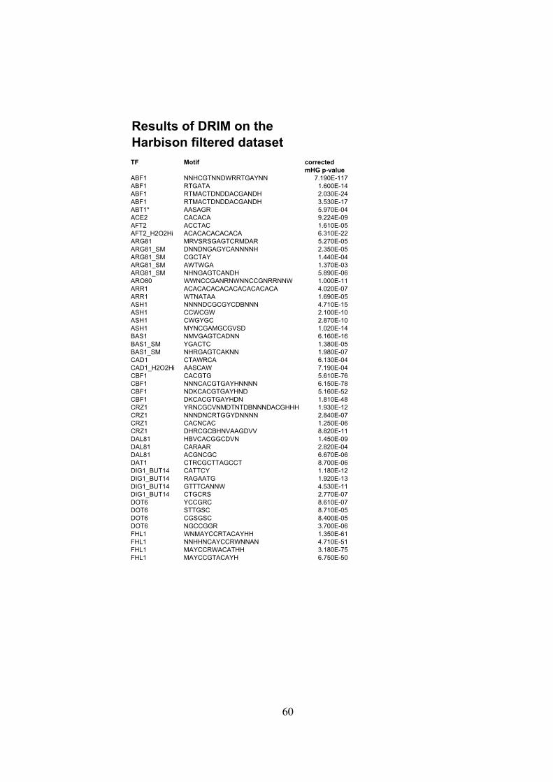
Results of DRIM on the
Harbison filtered dataset
TF Motif corrected
mHG p-value
ABF1 NNHCGTNNDWRRTGAYNN 7.190E-117
ABF1 RTGATA 1.600E-14
ABF1 RTMACTDNDDACGANDH 2.030E-24
ABF1 RTMACTDNDDACGANDH 3.530E-17
ABT1* AASAGR 5.970E-04
ACE2 CACACA 9.224E-09
AFT2 ACCTAC 1.610E-05
AFT2_H2O2Hi ACACACACACACA 6.310E-22
ARG81 MRVSRSGAGTCRMDAR 5.270E-05
ARG81_SM DNNDNGAGYCANNNNH 2.350E-05
ARG81_SM CGCTAY 1.440E-04
ARG81_SM AWTWGA 1.370E-03
ARG81_SM NHNGAGTCANDH 5.890E-06
ARO80 WWNCCGANRNWNNCCGNRRNNW 1.000E-11
ARR1 ACACACACACACACACACACA 4.020E-07
ARR1 WTNATAA 1.690E-05
ASH1 NNNNDCGCGYCDBNNN 4.710E-15
ASH1 CCWCGW 2.100E-10
ASH1 CWGYGC 2.870E-10
ASH1 MYNCGAMGCGVSD 1.020E-14
BAS1 NMVGAGTCADNN 6.160E-16
BAS1_SM YGACTC 1.380E-05
BAS1_SM NHRGAGTCAKNN 1.980E-07
CAD1 CTAWRCA 6.130E-04
CAD1_H2O2Hi AASCAW 7.190E-04
CBF1 CACGTG 5.610E-76
CBF1 NNNCACGTGAYHNNNN 6.150E-78
CBF1 NDKCACGTGAYHND 5.160E-52
CBF1 DKCACGTGAYHDN 1.810E-48
CRZ1 YRNCGCVNMDTNTDBNNNDACGHHH 1.930E-12
CRZ1 NNNDNCRTGGYDNNNN 2.840E-07
CRZ1 CACNCAC 1.250E-06
CRZ1 DHRCGCBHNVAAGDVV 8.820E-11
DAL81 HBVCACGGCDVN 1.450E-09
DAL81 CARAAR 2.820E-04
DAL81 ACGNCGC 6.670E-06
DAT1 CTRCGCTTAGCCT 8.700E-06
DIG1_BUT14 CATTCY 1.180E-12
DIG1_BUT14 RAGAATG 1.920E-13
DIG1_BUT14 GTTTCANNW 4.530E-11
DIG1_BUT14 CTGCRS 2.770E-07
DOT6 YCCGRC 8.610E-07
DOT6 STTGSC 8.710E-05
DOT6 CGSGSC 8.400E-05
DOT6 NGCCGGR 3.700E-06
FHL1 WNMAYCCRTACAYHH 1.350E-61
FHL1 NNHHNCAYCCRWNNAN 4.710E-51
FHL1 MAYCCRWACATHH 3.180E-75
FHL1 MAYCCGTACAYH 6.750E-50
60
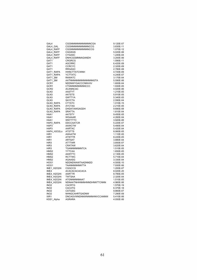
GAL4 CGGNNNNNNNNNNNNCGA 9.120E-07
GAL4_GAL CGGNNNNNNNNNNNCCG 3.830E-11
GAL4_RAFF CGGNNNNNNNNNNNCCG 1.070E-12
GAL4_RAFF CGGSGS 5.020E-06
GAL4_RAFF CYGASC 1.240E-04
GAL4_RAFF DNHCGGMNNAGANDH 3.200E-06
GAT1 CRGRCG 1.590E-11
GAT1 AGCRRC 6.420E-09
GAT1 CCRCYC 2.320E-09
GAT1 RRGAGC 2.780E-08
GAT1_RAPA HHNCTTATCWNH 4.720E-09
GAT1_RAPA YCTTATC 4.240E-07
GAT1_SM RAWATC 3.170E-04
GAT1_SM AATNNNNNNNNNNNNNNGTA 5.590E-06
GCR1 NDDNWYGACCCNNVHV 1.600E-04
GCR1 CTGNNNNNNNNNCCC 1.930E-05
GCR2 ACANNCAC 4.020E-06
GLN3 AASTYT 1.210E-05
GLN3 AATSTS 5.910E-05
GLN3 GWTTYA 5.340E-05
GLN3 SAYCTA 2.590E-04
GLN3_RAPA CTTATC 1.010E-15
GLN3_RAPA AYCTAA 2.210E-05
GLN3_RAPA DHDATAWGAGDH 9.680E-08
GLN3_RAPA SRATTA 1.810E-04
HAA1 AATSTY 9.450E-05
HAA1 WGAAAR 4.260E-04
HAA1 WNTTTTC 3.920E-06
HAP2_RAPA DDCCAATCR 5.220E-07
HAP3 AAWCTW 5.490E-04
HAP3 AARTAC 5.420E-04
HAP4_H2O2Lo ATSTTS 8.060E-05
HIR1 AWAATW 1.110E-05
HIR1 ATWTTR 8.220E-05
HIR1 ARTSAT 3.880E-04
HIR3 ATTTWR 3.850E-07
HIR3 CRATAW 3.620E-04
HIR3 TGANNNNNNNTCA 1.510E-05
HMS2 YYTCAA 1.650E-05
HMS2 AAWYTC 2.130E-05
HMS2 RCTTWC 5.710E-04
HMS2 AGAASG 3.330E-04
HOG1 NDDNDWAWTAADNNDD 4.500E-10
HOG1 TAANNNNNNNTTA 7.930E-06
IME1_H2O2Hi CGGCCG 1.200E-07
IME4 ACACACACACACA 8.020E-20
IME4_H2O2Hi AARTTR 8.780E-05
IME4_H2O2Hi TWTSAA 2.320E-04
IME4_H2O2Hi ATGNNNNNNAAT 1.510E-05
IME4_H2O2Hi NDNAATNHHNNNHNNDHNNTTCNNN 4.960E-06
INO2 CACRTG 1.570E-19
INO2 CACATG 6.370E-18
INO2 CSTGSG 9.860E-07
INO2 NHNGCAHRTGADNW 7.290E-09
IXR1 DNCAGVWNDNNWNNNNHNVCCANNW 5.410E-06
KSS1_Alpha AGRARA 4.050E-06
61
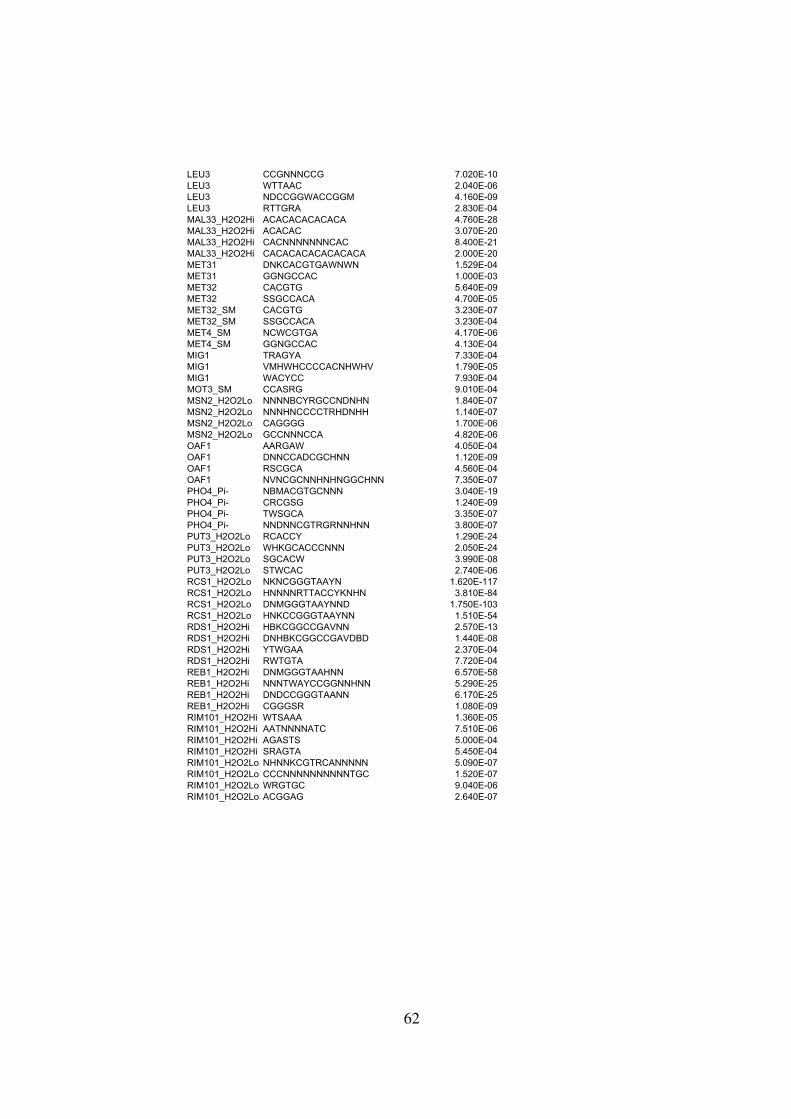
LEU3 CCGNNNCCG 7.020E-10
LEU3 WTTAAC 2.040E-06
LEU3 NDCCGGWACCGGM 4.160E-09
LEU3 RTTGRA 2.830E-04
MAL33_H2O2Hi ACACACACACACA 4.760E-28
MAL33_H2O2Hi ACACAC 3.070E-20
MAL33_H2O2Hi CACNNNNNNNCAC 8.400E-21
MAL33_H2O2Hi CACACACACACACACA 2.000E-20
MET31 DNKCACGTGAWNWN 1.529E-04
MET31 GGNGCCAC 1.000E-03
MET32 CACGTG 5.640E-09
MET32 SSGCCACA 4.700E-05
MET32_SM CACGTG 3.230E-07
MET32_SM SSGCCACA 3.230E-04
MET4_SM NCWCGTGA 4.170E-06
MET4_SM GGNGCCAC 4.130E-04
MIG1 TRAGYA 7.330E-04
MIG1 VMHWHCCCCACNHWHV 1.790E-05
MIG1 WACYCC 7.930E-04
MOT3_SM CCASRG 9.010E-04
MSN2_H2O2Lo NNNNBCYRGCCNDNHN 1.840E-07
MSN2_H2O2Lo NNNHNCCCCTRHDNHH 1.140E-07
MSN2_H2O2Lo CAGGGG 1.700E-06
MSN2_H2O2Lo GCCNNNCCA 4.820E-06
OAF1 AARGAW 4.050E-04
OAF1 DNNCCADCGCHNN 1.120E-09
OAF1 RSCGCA 4.560E-04
OAF1 NVNCGCNNHNHNGGCHNN 7.350E-07
PHO4_Pi- NBMACGTGCNNN 3.040E-19
PHO4_Pi- CRCGSG 1.240E-09
PHO4_Pi- TWSGCA 3.350E-07
PHO4_Pi- NNDNNCGTRGRNNHNN 3.800E-07
PUT3_H2O2Lo RCACCY 1.290E-24
PUT3_H2O2Lo WHKGCACCCNNN 2.050E-24
PUT3_H2O2Lo SGCACW 3.990E-08
PUT3_H2O2Lo STWCAC 2.740E-06
RCS1_H2O2Lo NKNCGGGTAAYN 1.620E-117
RCS1_H2O2Lo HNNNNRTTACCYKNHN 3.810E-84
RCS1_H2O2Lo DNMGGGTAAYNND 1.750E-103
RCS1_H2O2Lo HNKCCGGGTAAYNN 1.510E-54
RDS1_H2O2Hi HBKCGGCCGAVNN 2.570E-13
RDS1_H2O2Hi DNHBKCGGCCGAVDBD 1.440E-08
RDS1_H2O2Hi YTWGAA 2.370E-04
RDS1_H2O2Hi RWTGTA 7.720E-04
REB1_H2O2Hi DNMGGGTAAHNN 6.570E-58
REB1_H2O2Hi NNNTWAYCCGGNNHNN 5.290E-25
REB1_H2O2Hi DNDCCGGGTAANN 6.170E-25
REB1_H2O2Hi CGGGSR 1.080E-09
RIM101_H2O2Hi WTSAAA 1.360E-05
RIM101_H2O2Hi AATNNNNATC 7.510E-06
RIM101_H2O2Hi AGASTS 5.000E-04
RIM101_H2O2Hi SRAGTA 5.450E-04
RIM101_H2O2Lo NHNNKCGTRCANNNNN 5.090E-07
RIM101_H2O2Lo CCCNNNNNNNNNNTGC 1.520E-07
RIM101_H2O2Lo WRGTGC 9.040E-06
RIM101_H2O2Lo ACGGAG 2.640E-07
62
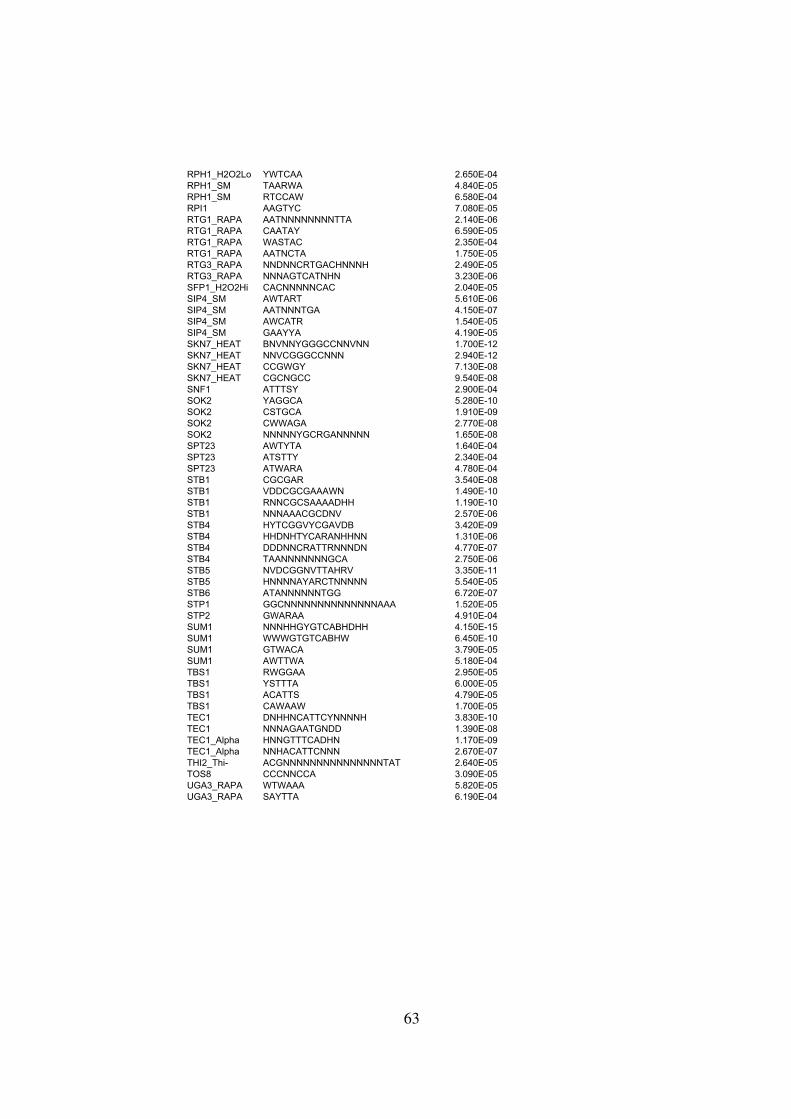
RPH1_H2O2Lo YWTCAA 2.650E-04
RPH1_SM TAARWA 4.840E-05
RPH1_SM RTCCAW 6.580E-04
RPI1 AAGTYC 7.080E-05
RTG1_RAPA AATNNNNNNNNTTA 2.140E-06
RTG1_RAPA CAATAY 6.590E-05
RTG1_RAPA WASTAC 2.350E-04
RTG1_RAPA AATNCTA 1.750E-05
RTG3_RAPA NNDNNCRTGACHNNNH 2.490E-05
RTG3_RAPA NNNAGTCATNHN 3.230E-06
SFP1_H2O2Hi CACNNNNNCAC 2.040E-05
SIP4_SM AWTART 5.610E-06
SIP4_SM AATNNNTGA 4.150E-07
SIP4_SM AWCATR 1.540E-05
SIP4_SM GAAYYA 4.190E-05
SKN7_HEAT BNVNNYGGGCCNNVNN 1.700E-12
SKN7_HEAT NNVCGGGCCNNN 2.940E-12
SKN7_HEAT CCGWGY 7.130E-08
SKN7_HEAT CGCNGCC 9.540E-08
SNF1 ATTTSY 2.900E-04
SOK2 YAGGCA 5.280E-10
SOK2 CSTGCA 1.910E-09
SOK2 CWWAGA 2.770E-08
SOK2 NNNNNYGCRGANNNNN 1.650E-08
SPT23 AWTYTA 1.640E-04
SPT23 ATSTTY 2.340E-04
SPT23 ATWARA 4.780E-04
STB1 CGCGAR 3.540E-08
STB1 VDDCGCGAAAWN 1.490E-10
STB1 RNNCGCSAAAADHH 1.190E-10
STB1 NNNAAACGCDNV 2.570E-06
STB4 HYTCGGVYCGAVDB 3.420E-09
STB4 HHDNHTYCARANHHNN 1.310E-06
STB4 DDDNNCRATTRNNNDN 4.770E-07
STB4 TAANNNNNNNGCA 2.750E-06
STB5 NVDCGGNVTTAHRV 3.350E-11
STB5 HNNNNAYARCTNNNNN 5.540E-05
STB6 ATANNNNNNTGG 6.720E-07
STP1 GGCNNNNNNNNNNNNNNAAA 1.520E-05
STP2 GWARAA 4.910E-04
SUM1 NNNHHGYGTCABHDHH 4.150E-15
SUM1 WWWGTGTCABHW 6.450E-10
SUM1 GTWACA 3.790E-05
SUM1 AWTTWA 5.180E-04
TBS1 RWGGAA 2.950E-05
TBS1 YSTTTA 6.000E-05
TBS1 ACATTS 4.790E-05
TBS1 CAWAAW 1.700E-05
TEC1 DNHHNCATTCYNNNNH 3.830E-10
TEC1 NNNAGAATGNDD 1.390E-08
TEC1_Alpha HNNGTTTCADHN 1.170E-09
TEC1_Alpha NNHACATTCNNN 2.670E-07
THI2_Thi- ACGNNNNNNNNNNNNNNNTAT 2.640E-05
TOS8 CCCNNCCA 3.090E-05
UGA3_RAPA WTWAAA 5.820E-05
UGA3_RAPA SAYTTA 6.190E-04
63
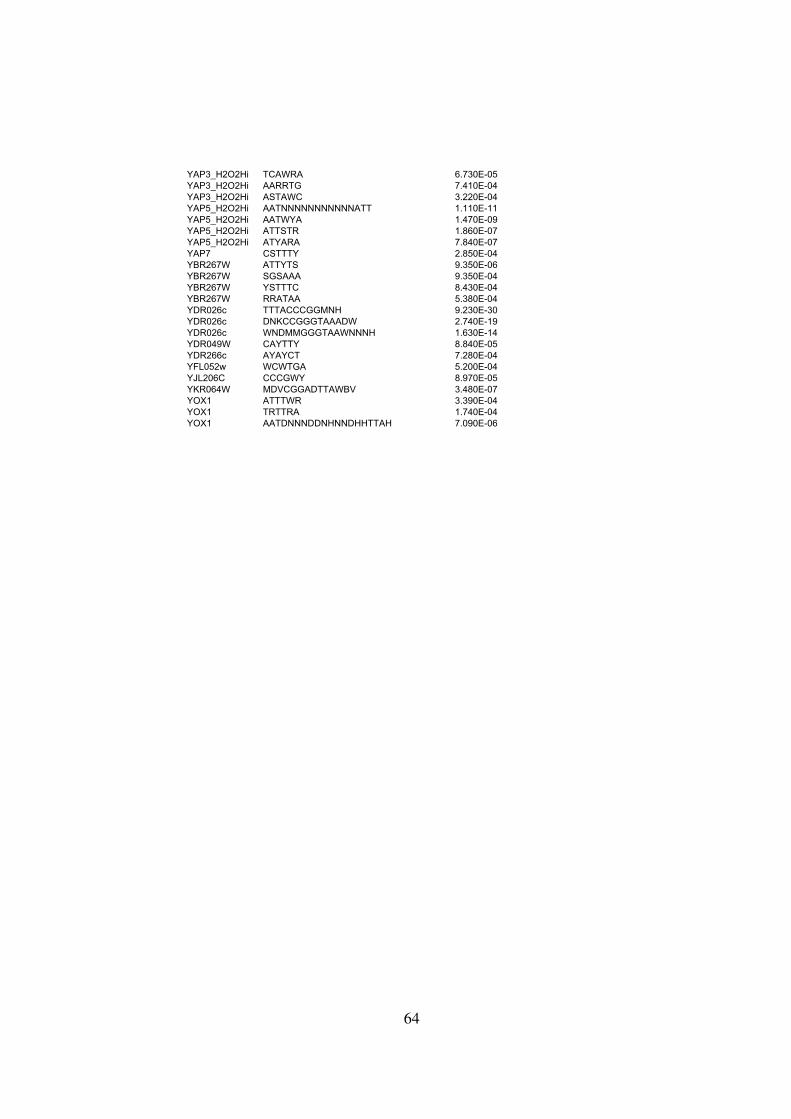
YAP3_H2O2Hi TCAWRA 6.730E-05
YAP3_H2O2Hi AARRTG 7.410E-04
YAP3_H2O2Hi ASTAWC 3.220E-04
YAP5_H2O2Hi AATNNNNNNNNNNNATT 1.110E-11
YAP5_H2O2Hi AATWYA 1.470E-09
YAP5_H2O2Hi ATTSTR 1.860E-07
YAP5_H2O2Hi ATYARA 7.840E-07
YAP7 CSTTTY 2.850E-04
YBR267W ATTYTS 9.350E-06
YBR267W SGSAAA 9.350E-04
YBR267W YSTTTC 8.430E-04
YBR267W RRATAA 5.380E-04
YDR026c TTTACCCGGMNH 9.230E-30
YDR026c DNKCCGGGTAAADW 2.740E-19
YDR026c WNDMMGGGTAAWNNNH 1.630E-14
YDR049W CAYTTY 8.840E-05
YDR266c AYAYCT 7.280E-04
YFL052w WCWTGA 5.200E-04
YJL206C CCCGWY 8.970E-05
YKR064W MDVCGGADTTAWBV 3.480E-07
YOX1 ATTTWR 3.390E-04
YOX1 TRTTRA 1.740E-04
YOX1 AATDNNNDDNHNNDHHTTAH 7.090E-06
64
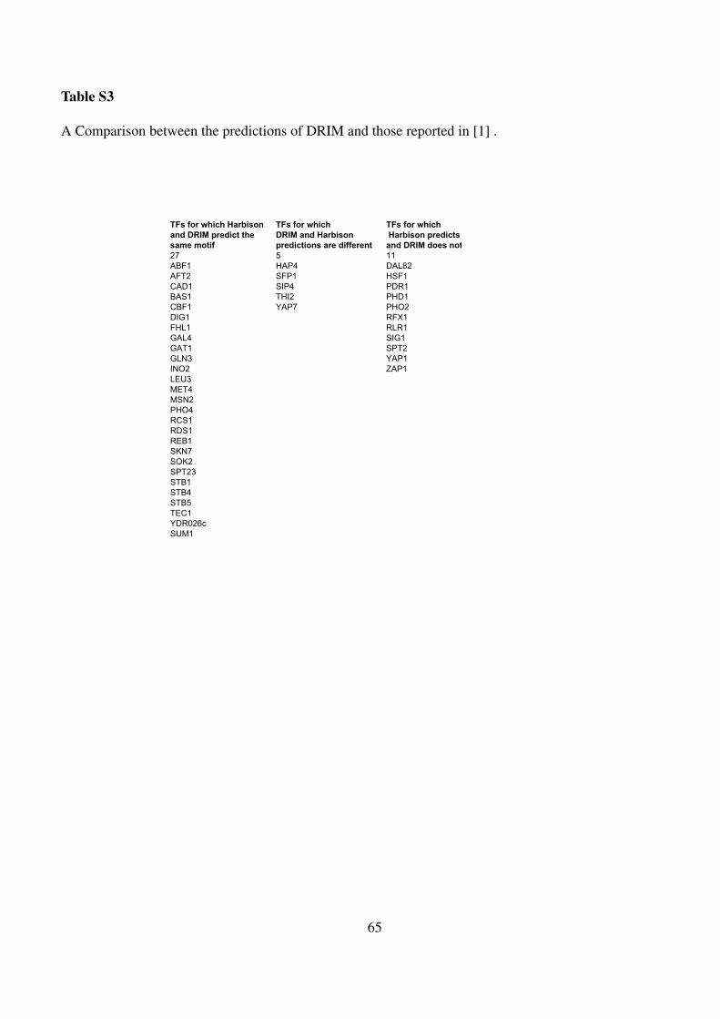
Table S3
A Comparison between the predictions of DRIM and those reported in [1] .
TFs for which Harbison TFs for which TFs for which
and DRIM predict the DRIM and Harbison Harbison predicts
same motif predictions are different and DRIM does not
27 5 11
ABF1 HAP4 DAL82
AFT2 SFP1 HSF1
CAD1 SIP4 PDR1
BAS1 THI2 PHD1
CBF1 YAP7 PHO2
DIG1 RFX1
FHL1 RLR1
GAL4 SIG1
GAT1 SPT2
GLN3 YAP1
INO2 ZAP1
LEU3
MET4
MSN2
PHO4
RCS1
RDS1
REB1
SKN7
SOK2
SPT23
STB1
STB4
STB5
TEC1
YDR026c
SUM1
65

Table S4
A Comparison between mHG flexible cutoffs and 10−3 fixed cutoffs in yeast ChIP-chip data.
Comparison between the number of promoters for which the
binding signal < 10−3 (denoted #(10−3)) with the number
of promoters at which mHG was attained in yeast ChIP-chip data.
fixed mHG optimal
TF name #p<0.001 threshold
ABF1 180 97
AFT2 20 97
AFT2H2O2hi 51 90
BAS1 39 87
CBF1 10 93
FHL1 133 99
GAL4 16 19
GAT1 8 99
GLN3_RAPA 79 57
HAP3 30 67
INO2 36 19
Leu3 31 22
MSN_H2O2Lo 74 99
SOK2 0 75
STB1 22 15
SUM1 54 92
TEC1 37 85
YDR026c 16 69
RDS1_H2O2Hi 52 45
REB1_H2O2hi 49 87
66
8 Appendix II - List of publications (during M.Sc. period):
• Eran Eden, Doron Lipson, Sivan Yogev and Zohar Yakhini. Discovering Sequence Motifs in Ranked
Lists of DNA Seqeunces. PLoS Computational Biology, 2007.
• Yeshayahu Schlesinger, Ravid Straussman, Ilana Keshet, Shlomit Farkash, Merav Hecht, Joseph Zim-
merman, Eran Eden, Zohar Yakhini, Etti Ben-Shushan, Benjamin E Reubinoff, Yehudit Bergman, Ita-
mar Simon, Howard Cedar. Polycomb mediated histone H3(K27) methylation pre-marks genes for
de-novo methylation in cancer. Nature Genetics, 2007
• Eran Eden, Michael Rudzsky, Vera Brod, Dan Waisman, Haim Bitterman, Edmond Sabo and Ehud
Rivlin. An automated method for analysis of blood cell flow characteristics from in-vivo video-
microscopic studies. IEEE, Transactions on Medical Imaging, vol. 24 Issue: 8, pp. 1011- 1024,
2005.
9 Appendix III - Web servers and software (during M.Sc. period):
• DRIM - the software is publicly available via an easy to use web interface:
http://bioinfo.cs.technion.ac.il/drim. Due to running time considerations the web service has restric-
tions on the number and length of the DNA sequences in the query. The exhaustive motif search space
is also restricted. These restrictions can be removed by downloading a local copy of DRIM. For more
details please see website.
• GOviz - the mHG based GO analysis and graphical visualization tool is available via the following web
interface: http://bioinfo.cs.technion.ac.il/GOviz
• SimTree - a tool for comparing RNA secondary structures is available via the following web interface:
http://bioinfo.cs.technion.ac.il/SimTree/
67