discovering of association rules without a minimum support...
TRANSCRIPT

Discovering of Association Rules
without a Minimum Support
Threshold –
Coherent Rules Discovery
by
Alex Tze Hiang Sim
BSc. (Hons), MSc. (IT), MBS
Dissertation submitted in fulfilment of the
requirements for the degree of
Doctor of Philosophy
Faculty of Information Technology
Monash University
Australia
March 2009

i
DECLARATION
In accordance with Monash University Doctorate Regulation 17 / Doctor of
Philosophy and Master of Philosophy (MPhil) regulations the following
declarations are made:
I hereby declare that this thesis contains no material which has been accepted
for the award of any other degree of diploma at any university or equivalence
institution and that, to the best of my knowledge and belief, this thesis contains
no material previously published or written by another person, except where
due references is made in the text of the thesis.
Alex Tze Hiang, Sim
Date: ___ / ___ / ______

ii
ACKNOWLEDGEMENTS
First of all, I would like to acknowledge Dr. Maria Indrawan whose passion it is
to teach and lead young researchers like me. She showed faith and great
determination in helping me during the various stages of my research. She has
been an excellent teacher and a model to me. I would also like to thank
Professor Bala Srinivasan, my second supervisor. I am very grateful for the
guidance and help he extended to me far beyond call of the duty. I learnt much
from both of them and they inspire me constantly.
I would also like to specially acknowledge Dr. Samar Zutshi. I very much
appreciate our discussions and encouragement in low times during the
research. Annette Lam is another friend who always brought up ideas for me to
think about away from my research, as well as other research friends Cheah
from Melbourne University, Viranga, Khai, Linyi, Ming, Ping, Abdul-Gapar, Tony,
Harry, Dr. Jenny, Kim, Nick, Dr. Flora and Dr Wen-Kai.
I am thankful for the friendships, prayer and financial support from the
Caulfield / Elwood Presbyterian Church. Special thanks to Dr. Sam and Rebecca
Lim and Auntie Ai Ling for care and support, Morris and King Goldberg’s family
for Christmas dinners and use of their car to travel from campus on winter
nights, Alfred and Lilian Ong for my daughter’s baby bed and clothes, Fred Lake,
Robert Beelcher, Sunny Lim, Dr Fee and Jean Gooey for sharing their
experiences and advice; Lydia Chang, Jenny Lim, Lynus Wong, Karen Wong, Keat
Chong and Doris Lim for delicious food, and Ilda Come, Joe Chong, Charles Liu
and Susan Sun for warm fellowship. I also cherish the care and sermons from a
number of pastors include Rev. Philip Chang, Rev. Evan Prentice, Rev. Professor

iii
Douglas Milne, Rev. Dr. Tony Bird, Rev. Dr. Botros Botrosdief and Rev. Dr.
Robert Carner. I thank my brother Dennis Sim, sister Corrina Sim, overseas /
interstate friends and former colleagues for encouragement and support. To
name a few, Mdm. Phang, Mdm. Loh, Sai Ming, families and friends from the
Holy Light Presbyterian Church in Malaysia, Professor Ahmad Zaki and Professor
Abdul Manan.
I thank my wife, Jee Mei for her constant support, love and sacrifice in
taking care of me and my daughter especially during the last one and a half
years when she had to stay overseas doing her PhD at a distance while taking
care of our daughter by herself.
I acknowledge and thank a number of proofreading done by Annette Lam,
Samar Zutshi and my supervisors on thesis drafts, conference and journal
papers. Finally, I acknowledge the financial support from Monash University
and administration support from the Research Graduate School Committee,
Michelle Ketchen, Allison Mitchell, Katherine Knight, Aleisha Matthews,
Akamon Kunkangkopun, Dianna Sussman, Julie Austin, Duke Fonias, See Ngieng,
Rafig Tjahjadi, Michael Leung and Ian Ng.

iv
DEDICATION
To Him who enabled me in this research.
And, in memory of my beloved parents who emphasised education.

v
LIST OF PUBLICATIONS
Book Chapter
1. Sim, A. T. H., Zutshi, S., Indrawan, M., & Srinivasan, B. (2009).
Discovering knowledge of association using coherent rules. In Trends in
Communication Technologies and Engineering Science: Springer, Ch. 24
(to appear).
Journals
1. Sim, A. T. H., Zutshi, S., Indrawan, M., & Srinivasan, B. (2008). The
discovery of coherent rules. IAENG International Journal of Computer
Science, 35(3), pp. 403-412.
2. Sim, A. T. H., Indrawan, M., & Srinivasan, B. (2008). The importance of
negative associations and the discovery of association rule pairs.
International Journal of Business Intelligence and Data Mining (IJBIDM),
3(2), pp. 158-176.
International Conferences
1. Sim, A. T. H., Indrawan, M., & Srinivasan, B. (2008). A threshold free
implication rule mining. Proceedings of the IAENG International
Conference on Data Mining and Applications (ICDMA). pp. 578-583
(awarded as the best paper of this conference).

vi
2. Sim, A. T. H., Indrawan, M., & Srinivasan, B. (2007). Importance of
negative associations and mining of association pairs. Proceedings of the
9th International Conference on Information Integration and Web-based
Applications Services (IIWAS). pp. 169-178.
3. Sim, A. T. H., Indrawan, M., & Srinivasan, B. (2008). Mining infrequent
and interesting rules from transaction records. Proceedings of the
Advances on Artificial Intelligence, Knowledge Engineering, and Data
Bases (AIKED). pp. 515-520.

vii
ABSTRACT
In the data mining field, association rules have been researched for more
than fifteen years; however, the degree to which the support threshold
effectively discovers interesting association rules has received little attention.
This thesis proposes a new framework for data mining through which
interesting association rules called coherent rules can be discovered. Coherent
rules are those associations that can be mapped to logical equivalences
according to propositional logic. Hence, coherent rules can be reasoned as
logically true statements based solely on the truth table values of logical
equivalence.
Discovering coherent rules resolves the many difficulties in mining
associations that require a preset minimum support threshold. Apart from
solving the issues of a support threshold, the coherent rules found can also be
reasoned as logical implications due to the mapping to the truth table values of
logical equivalence. In contrast, classic association rules cannot be reasoned as
logical implications due to their lack of this logic property.
We have further devised a measure of interestingness to use with coherent
rules that quantifies a coherent rule implicational strength value. The
interestingness measure is sensitive to the direction of an implication. Use of
coherent rules together with the measure of interestingness provides us with a
better representation of associations in data mining due to their logical
implications and unidirectional properties.
An algorithm to discover coherent rules is also presented in this thesis. The
algorithm was designed to find the shortest and strongest rule or most effectual

viii
coherent rules by exploiting the properties of coherent rules. Decision or
actions can be implemented based on these coherent rules. In a situation
whereby users are interested in weaker and/or longer rules, the algorithm
enables parameters to be set. Unlike support threshold settings, these
parameters do not require users to have prior knowledge of the context in
which the data mining takes place.
We have tested our framework on several datasets. The results confirm the
strength of coherent rules in finding association rules that can be reasoned
logically and in finding association rules that consider both infrequent items and
negative associations. The algorithm used to discover coherent rules is also
efficient. This was demonstrated by the number of prunings made to the search
space during the discovery process.
This study suggests that our framework for discovering coherent rules
offers a technique for data mining that overcomes the limitations associated
with existing methods and enables the finding of association rules among the
presence and/or absence of a set of items without a preset minimum support
threshold. The results justify continuing research in this area in order to
increase the body of scientific knowledge of data mining – and specifically,
association rules - and to provide practical support to those involved in data
mining activities.

ix
TABLE OF CONTENTS
Declaration ............................................................................. i
Acknowledgements .............................................................................ii
Dedication ............................................................................ iv
List of Publications ............................................................................. v
Abstract ........................................................................... vii
Table of Contents ............................................................................ ix
List of Figures ........................................................................... xv
List of Tables ......................................................................... xvii
Chapter 1 Introduction ................................................................. 1
1.1 Preamble ................................................................................................1
1.2 Market Basket Analysis ...........................................................................2
1.3 Motivation..............................................................................................4
1.4 Research Objectives, Contributions and Scope ........................................5
1.5 Organisation of Dissertation ...................................................................8
Chapter 2 Market Basket Analysis ............................................. 11
2.1 Introduction ......................................................................................... 11
2.2 Preliminaries ........................................................................................ 12
2.2.1 Terminologies ....................................................................................... 14

x
2.3 Issues with a Preset Minimum Support Threshold ................................. 18
2.3.1 Loss of Association Rules involving Frequent Items in setting a
Minimum Support Threshold ............................................................... 19
2.3.2 Loss of Association Rules involving Infrequent Items .......................... 21
2.3.2.1 Association Rules Involving Rare Items .......................................... 21
2.3.2.2 Association Rules that are measured using other Measures
of Interestingness ........................................................................... 27
2.3.2.3 Negative Association Rules ............................................................. 32
2.4 A Potential Approach and the Measure of Interestingness .................... 39
2.4.1 Logical Implications ............................................................................... 40
2.4.1.1 Logical Implications to minimise Contradictions ............................ 42
2.4.2 Measure of Interestingness – Lambda ................................................. 43
2.5 Conclusion ............................................................................................ 45
Chapter 3 A Threshold-Free Rule Mining Framework ............ 47
3.1 Introduction ......................................................................................... 47
3.2 Association Rules and Implications ....................................................... 49
3.2.1 Differences in Relations ........................................................................ 50
3.2.1.1 A Rule .............................................................................................. 50
3.2.1.2 An Implication ................................................................................. 53
3.2.1.3 A Material Implication .................................................................... 54
3.2.1.4 An Equivalence ................................................................................ 55
3.3 Mapping Association Rules to Equivalences .......................................... 56
3.3.1 Mapping using a Single Transaction Record ......................................... 57

xi
3.3.2 Mapping using Multiple Transaction Records ...................................... 60
3.4 Concept of Coherent Rules .................................................................... 65
3.5 Finding Coherent Rules in Datasets ....................................................... 68
3.5.1 Coherent Rules in Transaction Records ................................................ 69
3.5.2 Finding Coherent Rules in Classification Datasets – Attributes
and Class Analysis ................................................................................. 73
3.6 Conclusion ............................................................................................ 77
Chapter 4 Mining Coherent Rules .............................................. 79
4.1 Introduction ......................................................................................... 79
4.2 Terminology and Considerations ........................................................... 80
4.2.1 Candidate Coherent Rules .................................................................... 80
4.2.2 Coherent Rules ...................................................................................... 82
4.2.3 Search Space for Coherent Rules .......................................................... 83
4.2.4 Constraints in Coherent Rules Discovery .............................................. 84
4.3 Coherent Rule Measure of Interestingness and Its Relevant
Properties .................................................................................................. 85
4.3.1 Properties of the Measure of Interestingness – 𝐿𝑎𝑚𝑏𝑑𝑎 ................... 86
4.3.2 Augmenting Measure Lambda as Measure of Interestingness 𝐻 ........ 90
4.3.3 The Effect of 𝐻 in the Design of the Mining Algorithm ........................ 94
4.4 Generating Candidate Coherent Rules .................................................. 95
4.5 Selectively Generating the Most Effectual Coherent Rules .................... 98
4.5.1 Finding Valid Coherent Rules ................................................................ 99
4.5.1.1 Changes in Support Values ............................................................. 99
4.5.1.2 An Anti-monotone Condition of Coherent Rules .........................105

xii
4.5.1.3 Generalising the Anti-monotone Conditions of Coherent
Rules .............................................................................................106
4.5.2 Finding the Strongest Coherent Rules ................................................108
4.5.2.1 Anti-monotone Property Absence and the Measure of
Interestingness .............................................................................108
4.5.2.2 Measure of Interestingness 𝐻′ .....................................................111
4.5.2.3 The Anti-monotone Property of the Measure of
Interestingness 𝐻′ ........................................................................115
4.5.2.4 Another Refinement of the Measure of Interestingness 𝐻′′ .......117
4.5.2.5 The Anti-monotone Property of the Measure of
Interestingness 𝐻′′ .......................................................................121
4.5.2.6 Finding the Strongest Strength Value ...........................................122
4.5.3 Finding the Shortest Coherent Rules ..................................................123
4.5.3.1 Strategy to Discover the Most Effectual Coherent Rules .............124
4.5.3.2 Coherent Rules Generation Algorithm (𝐺𝑆𝑆_𝐶𝑅) ........................128
4.6 An Extended Coherent Rules Generation Algorithm ............................ 132
4.6.1 Strength Value Window (𝑊)...............................................................132
4.6.2 Length Window (𝐿) .............................................................................133
4.6.3 The Algorithm 𝐸𝑆𝑆_𝐶𝑅 .......................................................................134
4.7 Conclusion .......................................................................................... 137
Chapter 5 Analysis of Performance .......................................... 139
5.1 Introduction ....................................................................................... 139
5.2 Preliminaries ...................................................................................... 141
5.2.1 Zoo Dataset .........................................................................................141

xiii
5.3 Goodness of Constraints ..................................................................... 143
5.3.1 Evaluation Measures...........................................................................143
5.3.2 Effect of Constraints ...........................................................................148
5.3.2.1 Effect of 𝐶3 ...................................................................................148
5.3.2.2 Effect of 𝐶1 ...................................................................................151
5.3.2.3 Effect of 𝐶2 ...................................................................................153
5.3.2.4 Effect of 𝐶4 ...................................................................................155
5.4 Quality of Coherent Rules ................................................................... 159
5.4.1 Infrequent Rules .................................................................................159
5.4.2 Frequent and Interesting Rules ..........................................................163
5.4.3 Negative Rules ....................................................................................167
5.4.4 Distinct Features of 𝐸𝑆𝑆_𝐶𝑅 ...............................................................170
5.5 𝑬𝑺𝑺_𝑪𝑹 Performance ......................................................................... 172
5.5.1 Effect of Parameter Values on the Number of Coherent Rules
Discovered ..........................................................................................172
5.5.2 Effect of Parameter 𝐿 Value vs. Time .................................................175
5.5.3 Effect of Parameter 𝑊 vs. Time ..........................................................180
5.5.4 Increase of Time over Number of Attribute Values ...........................186
5.6 Discovering Coherent Rules on Real-world Market Basket
Transaction Records ................................................................................. 189
5.6.1 Observations .......................................................................................191
5.6.2 Finding of Coherent Rules ...................................................................191
5.6.3 Finding of Infrequent and Negative Association Rules.......................193
5.7 Conclusion .......................................................................................... 196

xiv
Chapter 6 Conclusion ................................................................. 198
6.1 Research Summary ............................................................................. 198
6.2 Research Contributions ....................................................................... 200
6.3 Future Work ....................................................................................... 202
References ......................................................................... 205
Appendix A Finding Exclusive Conditions within the
Measure of 𝑳𝒂𝒎𝒃𝒅𝒂 ...................................... 220
Appendix B Properties of the Measure of
Interestingness 𝑯 .......................................... 225
Appendix C Description of Zoo Database ........................ 228
Appendix D Association Rules found on Infrequently
observed Class Values ................................... 232
Appendix E Residuals at varying Length Window 𝑳 ....... 236
Appendix F Residuals at varying Strength Value
Window 𝑾 ...................................................... 245

xv
LIST OF FIGURES
Figure 1.1 Framework of Mining Association Rules without using a Minimum Support Threshold
6
Figure 4.1 Fixed-structure to represent all Candidate Coherent Rules (𝐶𝐶𝑅)
96
Figure 4.2 Shortest and Strongest Coherent Rules Generation Algorithm (𝐺𝑆𝑆_𝐶𝑅)
131
Figure 4.3 Extended Shortest and Strongest Coherent Rules Generation Algorithm (𝐸𝑆𝑆_𝐶𝑅)
137
Figure 5.1 Number of Additional 𝐶𝐶𝑅 avoided in using 𝐶1 over 𝐶3 over Increasing 𝑊
152
Figure 5.2 Number of Additional 𝐶𝐶𝑅 avoided in using 𝐶2 over 𝐶3 over Increasing 𝑊
153
Figure 5.3 Number of Additional CCR avoided in using 𝐶4 over 𝐶3 155
Figure 5.4 Number of Coherent Rules discovered using different Parameter Values 𝐿 at W = 0
173
Figure 5.5 Number of Coherent Rules discovered using different Parameter Values 𝑊 at L = 0
173
Figure 5.6 Coherent Rules found, where 𝑌 = {′𝑟𝑒𝑝𝑡𝑖𝑙𝑒′} 175
Figure 5.7 Coherent Rules found, where 𝑌 = {′𝑚𝑎𝑚𝑚𝑎𝑙′} 176
Figure 5.8 Coherent Rules found, where 𝑌 = {′𝑖𝑛𝑣𝑒𝑟𝑡𝑒𝑏𝑟𝑎𝑡𝑒′} 176
Figure 5.9 Coherent Rules found, where 𝑌 = {′𝑖𝑛𝑠𝑒𝑐𝑡′} 177
Figure 5.10 Coherent Rules found, where 𝑌 = {′𝑓𝑖𝑠′} 177

xvi
Figure 5.11 Coherent Rules found, where 𝑌 = {′𝑏𝑖𝑟𝑑′} 178
Figure 5.12 Coherent Rules found, where 𝑌 = {′𝑎𝑚𝑝𝑖𝑏𝑖𝑎𝑛′} 178
Figure 5.13 Effect of 𝑊 vs. Time, where 𝑌 = {′𝑟𝑒𝑝𝑡𝑖𝑙𝑒′} 181
Figure 5.14 Effect of 𝑊 vs. Time, where 𝑌 = {′𝑚𝑎𝑚𝑚𝑎𝑙′} 181
Figure 5.15 Effect of 𝑊 vs. Time, where 𝑌 = {′𝑖𝑛𝑣𝑒𝑟𝑡𝑒𝑏𝑟𝑎𝑡𝑒′} 182
Figure 5.16 Effect of 𝑊 vs. Time, where 𝑌 = {′𝑖𝑛𝑠𝑒𝑐𝑡′} 182
Figure 5.17 Effect of 𝑊 vs. Time, where 𝑌 = {′𝑓𝑖𝑠′} 183
Figure 5.18 Effect of 𝑊 vs. Time, where 𝑌 = {′𝑏𝑖𝑟𝑑′} 183
Figure 5.19 Effect of 𝑊 vs. Time, where 𝑌 = {′𝑎𝑚𝑝𝑖𝑏𝑖𝑎𝑛′} 184
Figure 5.20 Increase in Time over Number of Attribute Values (𝑰) 186
Figure 5.21 Increase in Coherent Rules over Number of Attribute Values (𝑰)
187
Figure 6.1 Future Work based on Pseudo-implications 204

xvii
LIST OF TABLES
Table 2.1 Truth Table of a Material Implication 40
Table 3.1 Truth Table of a Material Implication 54
Table 3.2 Truth Table for an Equivalence 55
Table 3.3 Mapping of Association Rules to Equivalences 59
Table 3.4 Association Rules and Supports 62
Table 3.5 Artificial Transaction Records 71
Table 3.6 Contingency Table for 𝒊𝟏 and 𝒊𝟕 71
Table 3.7 Contingency Table for 𝒊𝟐 and 𝒊𝟕 72
Table 3.8 Five Coherent Rules Found 73
Table 3.9 Small Classification Dataset 75
Table 3.10 A Contingency Table for Milk and Mammal 76
Table 4.1 A Contingency Table for Variables A and B 91
Table 4.2 A Contingency Table for Categories 𝐴1 and 𝐵1 92
Table 4.3 A Contingency Table for Candidate Coherent Rules (𝑋. .𝑌) 101
Table 4.4 A Contingency Table for Candidate Coherent Rule (𝑋𝐸. .𝑌) 104
Table 4.5 Summary of Methods to generate the Shortest and Strongest Coherent Rules
124
Table 5.1 Summary of the Statistics for the Zoo Dataset 142

xviii
Table 5.2 Total Frequency of Class Attributes 142
Table 5.3 Number of Candidate Coherent Rules allowed after 𝐶3 150
Table 5.4 Number of Candidate Coherent Rules allowed after 𝐶3 at 𝑊 = 1
151
Table 5.5 Percentage of Additional Candidate Coherent Rules allowed in Addition to 𝐶3 at W = 0, 𝐿 = 0
157
Table 5.6 Shortest Infrequent Rules found on 𝑟𝑒𝑝𝑡𝑖𝑙𝑒 and 𝑎𝑚𝑝𝑖𝑏𝑖𝑎𝑛
160
Table 5.7 Shortest Frequent Rules found on Class 𝑚𝑎𝑚𝑚𝑎𝑙 163
Table 5.8 A Contingency Table for Attributes: domestic and mammal 164
Table 5.9 A Contingency Table for Attributes: breathes and mammal 164
Table 5.10 Shortest Negative Coherent Rules found, where 𝑌 = {′𝑚𝑎𝑚𝑚𝑎𝑙′}
168
Table 5.11 Shortest Negative Coherent Rules found, where 𝑌 = {′𝑟𝑒𝑝𝑡𝑖𝑙𝑒′} and 𝑌 = {′𝑎𝑚𝑝𝑖𝑏𝑖𝑎𝑛′}
169
Table 5.12 Summary of the Statistics on Transaction Records (TC) used
189
Table 5.13 Real-world Retail Transaction Records 190
Table 5.14 A Coherent Rules found in Retail transaction records 195
Table C-1 Class Attributes in Zoo Dataset 230
Table C-2 Attributes and their Attribute Values in Zoo Dataset 231
Table E-1 The Residuals at varying Parameter 𝐿 (𝑌 = {′𝑟𝑒𝑝𝑡𝑖𝑙𝑒′}, 1st Phase)
238
Table E-2 The Residuals at varying Parameter 𝐿 (𝑌 = {′𝑟𝑒𝑝𝑡𝑖𝑙𝑒′}, 2nd Phase)
238

xix
Table E-3 The Residuals at varying Parameter 𝐿 (𝑌 = {′𝑚𝑎𝑚𝑚𝑎𝑙′}, 1st Phase)
239
Table E-4 The Residuals at varying Parameter 𝐿 (𝑌 = {′𝑚𝑎𝑚𝑚𝑎𝑙′}, 2nd Phase)
239
Table E-5 The Residuals at varying Parameter 𝐿 (𝑌 = {′𝑖𝑛𝑣𝑒𝑟𝑡𝑒𝑏𝑟𝑎𝑡𝑒′}, 1st Phase)
240
Table E-6 The Residuals at varying Parameter 𝐿 (𝑌 = {′𝑖𝑛𝑣𝑒𝑟𝑡𝑒𝑏𝑟𝑎𝑡𝑒′}, 2nd Phase)
240
Table E-7 The Residuals at varying Parameter 𝐿 (𝑌 = {′𝑖𝑛𝑠𝑒𝑐𝑡′}, 1st Phase)
241
Table E-8 The Residuals at varying Parameter 𝐿 (𝑌 = {′𝑖𝑛𝑠𝑒𝑐𝑡′}, 2nd Phase)
241
Table E-9 The Residuals at varying Parameter 𝐿 (𝑌 = {′𝑓𝑖𝑠′}, 1st Phase)
242
Table E-10 The Residuals at varying Parameter 𝐿 (𝑌 = {′𝑓𝑖𝑠′}, 2nd Phase)
242
Table E-11 The Residuals at varying Parameter 𝐿 (𝑌 = {′𝑏𝑖𝑟𝑑′}, 1st Phase)
243
Table E-12 The Residuals at varying Parameter 𝐿 (𝑌 = {′𝑏𝑖𝑟𝑑′}, 2nd Phase)
243
Table E-13 The Residuals at varying Parameter 𝐿 (𝑌 = {′𝑎𝑚𝑝𝑖𝑏𝑖𝑎𝑛′}, 1st Phase)
244
Table E-14 The Residuals at varying Parameter 𝐿 (𝑌 = {′𝑎𝑚𝑝𝑖𝑏𝑖𝑎𝑛′}, 2nd Phase)
244
Table F-1 The Residuals at varying Parameter 𝐿 (𝑌 = {′𝑟𝑒𝑝𝑡𝑖𝑙𝑒′}, 1st Phase)
247
Table F-2 The Residuals at varying Parameter 𝐿 (𝑌 = {′𝑟𝑒𝑝𝑡𝑖𝑙𝑒′}, 2nd Phase)
247

xx
Table F-3 The Residuals at varying Parameter 𝐿 (𝑌 = {′𝑚𝑎𝑚𝑚𝑎𝑙′}, 1st Phase)
248
Table F-4 The Residuals at varying Parameter 𝐿 (𝑌 = {′𝑚𝑎𝑚𝑚𝑎𝑙′}, 2nd Phase)
248
Table F-5 The Residuals at varying Parameter 𝐿 (𝑌 = {′𝑖𝑛𝑣𝑒𝑟𝑡𝑒𝑏𝑟𝑎𝑡𝑒′}, 1st Phase)
249
Table F-6 The Residuals at varying Parameter 𝐿 (𝑌 = {′𝑖𝑛𝑣𝑒𝑟𝑡𝑒𝑏𝑟𝑎𝑡𝑒′}, 2nd Phase)
249
Table F-7 The Residuals at varying Parameter 𝐿 (𝑌 = {′𝑖𝑛𝑠𝑒𝑐𝑡′}, 1st Phase)
250
Table F-8 The Residuals at varying Parameter 𝐿 (𝑌 = {′𝑖𝑛𝑠𝑒𝑐𝑡′}, 2nd Phase)
250
Table F-9 The Residuals at varying Parameter 𝐿 (𝑌 = {′𝑓𝑖𝑠′}, 1st Phase)
251
Table F-10 The Residuals at varying Parameter 𝐿 (𝑌 = {′𝑓𝑖𝑠′}, 2nd Phase)
251
Table F-11 The Residuals at varying Parameter 𝐿 (𝑌 = {′𝑏𝑖𝑟𝑑′}, 1st Phase)
252
Table F-12 The Residuals at varying Parameter 𝐿 (𝑌 = {′𝑏𝑖𝑟𝑑′}, 2nd Phase)
252
Table F-13 The Residuals at varying Parameter 𝐿 (𝑌 = {′𝑎𝑚𝑝𝑖𝑏𝑖𝑎𝑛′}, 1st Phase)
253
Table F-14 The Residuals at varying Parameter 𝐿 (𝑌 = {′𝑎𝑚𝑝𝑖𝑏𝑖𝑎𝑛′}, 2nd Phase)
253

1
Chapter 1
INTRODUCTION
1.1 Preamble
With the birth of the computer researchers were given the power and
convenience to analyse and discover interesting and non-obvious knowledge
from large databases. The process of obtaining this knowledge via the computer
is known as Data Mining [WiFr05, pp. 4, 5].
The popularity and importance of data mining has its roots in two causes:
the ever-increasing volume of data and computation power. The amount of
information in the world doubles every twenty months [FrPiMa92]. Business
activities, for example, continue to produce an increasing stream of data (such
as point-of-sales transactions) which is stored in larger and cheaper data
storage. In the meantime, the computational power available continues to
increase. Gordon Moore, co-founder of the Intel corporation, points out that
the number of transistors on a chip doubles approximately every two years
[In05a], and that this trend has continued for more than half a century [In05b].
The consequence of the increasing volume of data and computational power is
an opportunity to create data mining applications based on state-of-art theories
and algorithms to discover interesting knowledge from large volumes of data.

2
1.2 Market Basket Analysis
A number of functions are used in data mining including, for example, link
analysis, prediction and visualisation. A link analysis typically discovers the
knowledge of “what goes with what” and “what follows what” [ShPaBr07],
[St08]. The latter is called sequence analysis and identifies a sequence of events,
while the former is known as affinity analysis.
An example of affinity analysis in the retail sector is the Market Basket
Analysis (MBA). Given a set of retail transaction records, a MBA finds
associations between the different items that customers place in their shopping
market baskets. Some items are often purchased together and other items are
not. For example, item A is often purchased together with item B. Finding these
associations helps to describe customers’ buying habits. Knowing such
associations helps a retailer to devise effective marketing strategies. A
promotion to increase the sale of any one item within an association could
increase the sales of another item.
One classic approach to discovering the patterns that go together is via the
support and confidence framework proposed by Agrawal, Imielinski and Swami
[AgImSw93]. Using this framework, patterns that can be observed frequently in
a set of transaction records are identified. To identify these patterns, the
framework requires a user to preset a threshold that segregates frequently
observed patterns from infrequent patterns. This threshold is called a minimum
support threshold. Later, a set of items that have appeared together above this
minimum support threshold are searched. Rules that connect two sets of
frequently observed items that have appeared together above a minimum
support threshold are found and, in many cases, a second measure of
interestingness such as confidence is used to further filter the rules found for

3
interesting association rules. This classic approach discovers the association
rules among the frequently observed patterns in a set of transaction records.
For more than 15 years, researchers have mostly proposed models to
discover association rules above a minimum support threshold. While searching
for association rules among frequent patterns is important, in some cases,
reporting the association rules among the items that fall below a minimum
support threshold are also important [LiHsMa99], [LiTsSu02], [YuHaHwRy03],
[HuCh06], [KoRoOk06a]. These unreported associations are considered to be
lost rules and need to be avoided to further improve data mining models. In
addition, the separation of frequent and infrequent items by a support
threshold prevents associations from being made between frequent and
infrequent items which, in some cases, are useful [KoRoOk06b], [KoRoOk08]. In
addition, typical association rule mining models are applied to items that can be
observed frequently over a set of transaction records. The relationships with, or
among, the absence of items observed over a set of transaction records are not
mined. Consequently, the association rules discovered are mostly incomplete
and disadvantageous. These facts have shaped our motivation for this thesis.
Our motivation is further detailed in the next section by highlighting the
disadvantages and type of rule loss.

4
1.3 Motivation
Discovering a complete set of associations is desirable in data mining. The
adverse effects of making decision based on incomplete information can be
costly to an organisation. The adverse effects are a consequence of the
following reasons:
(i) It is misleading to report an incomplete set of rules and at the
same time create a sense that all available rules have been found.
This situation misleads a decision maker into thinking that only
these rules are available which in turn will lead a decision maker to
reason with incomplete information. Reasoning with incomplete
information while not knowing that it is incomplete may lead to
inappropriate decisions.
(ii) Due to the large amount of rules available, a user often configures
an association rule mining algorithm to output only the strongest
rules. It is risky to make analysis based on the reporting of the
strongest available rules from the computational search that does
not cover a complete set of rules. There is no guarantee that the
strongest association rules found are indeed the strongest when
other rules that may be hidden are considered. It is possible that
the strongest rule lies among the hidden rules. This situation can
again lead to a decision making unknowingly drawing erroneous
conclusions about the relationship among items in a dataset.
(iii) Reporting an association that ignores the absence of items in a
given transaction record during the data mining process is
misleading. For example, to report that item 𝐴 is associated with
item 𝐵 is misleading if a stronger association can be found

5
between item 𝐴 and the absence of item 𝐵. Again, inappropriate
decisions may be made as a consequence.
The above reasons motivated us to seek for a complete set of association
rules that include association rules involving infrequently observed items and
absent items in each transaction record. In addition, if we could identify
interesting association rules from a dataset without having to supply a
minimum support threshold, then the adverse effect of missing association
rules could be offset. We were thus interested in designing an alternative
framework to discover interesting association rules without a preset minimum
support threshold.
1.4 Research Objectives, Contributions and Scope
The aim of our research was to develop a framework of association rule
mining that is data oriented and possesses two important properties:
(i) The algorithm that discovers the association rules should not rely
on a minimum support threshold, and
(ii) The pattern should consider both the presence and absence of a
set of items.
To achieve this objective, a new data mining framework to discover interesting
patterns according to propositional logic is proposed. Because the pattern is
discovered based on propositional logic, no support threshold needs to be set.
In addition, both the presence and absence of items are considered during the
design of the framework.
The patterns discovered by the framework are called coherent rules. Unlike
association rules, a coherent rule is made up of a pair of rules. Each member of
this pair is an association rule. The framework takes the pattern further by

6
mapping these association rules to propositional logic implications to generate
pseudo implication rules. Further mapping is them performed to the rules
based on a specific mode of implication in propositional logic, such as logical
equivalence. We depict the framework of mapping in Figure 1.1.
Figure 1.1: Framework of Mining Association Rules without using a Minimum
Support Threshold
Our proposed framework provides a means to map association rules to
implications according to propositional logic and provides a solution for mining
association rules without a minimum support threshold. Based on Figure 1.1,
the mapping from association rules to implications is two-fold. First, association
rules are mapped to implications in propositional logic and are called pseudo-
implications. Second, we further map pseudo-implications to a specific mode of

7
implication. While there are many modes of implication in propositional logic,
we have chosen (logical) equivalences in propositional logic. An equivalence is
more stringent in implication compared to other modes such as material
implication. Having mapped pseudo-implications to equivalences, these
pseudo-implications have the same truth table values as equivalences.
Consequently, the resulting rules can be considered to be logically true
according to the truth table values of equivalence.
This dissertation, based on the proposed framework, makes the following
contributions:
(i) It provides a definition of a coherent rule in which the rule is
reported based on the statistics of the presence and absence of
items, and also the truth table value of a logical equivalence.
(ii) It provides a measure that quantifies the implicational strength of
a coherent rule based on the concept of proportional error
reduction. This measure has two properties:
(a) it is asymmetrical because the unidirectional strength of a
coherent rule is quantified, and
(b) it considers the marginal probability of the consequence.
This measure allows comparison among coherent rules for the
stronger rules having the same consequence, and
(iii) It develops an algorithm based on the anti-monotone property of
coherent rules to discover the most interesting coherent rules.
This property allows the pruning of non-interesting rules during
the discovery of coherent rules. The algorithm utilised in our
proposed strategy needs neither to generate nor store a large
number of item sets in memory.

8
(iv) It extends the above algorithm to discover all coherent rules of
arbitrarily size and strength values in a dataset.
All contributions have been investigated and tested accordingly.
This research is necessarily confined within the scope of discovering a type
of interesting association rules from a dataset without using a minimum
support threshold. The following assumptions have been made in this work:
(i) A dataset can be loaded into memory. The assumption has been
made given that a large capacity for memory can now be made
available cheaply, where part or entire data is fitted into memory
such as in [BaAgGu99], [ChZa03], and [McCh07], and
(ii) Each rule consequence contains a single item that is pre-selected
from data similar to those suggested in [We95], [BaAgGu99],
[RaReWuPe04] and [CoTaTuXu05]. Our search has been to find a
combination of items for the left-hand side of a rule that is
associated with a single item on the right, without loss.
In the next section the structure of the dissertation is outlined.
1.5 Organisation of Dissertation
This thesis is organised as follows. Chapter 2 provides an overview and
explains the terminologies used in association rules discovery. Based on these
terminologies and overview, the chapter details the reasons for mining
association rules without having a minimum support threshold. We highlight
the types of association rules that are typically not mined, and discuss the
existing work to mine some of these missing association rules. At the end of this
chapter, we highlight a potential approach to mine association rules by
considering logical implications, and the concept of proportional error reduction,

9
which does not require a minimum support threshold to define the meaning of
association.
Chapter 3 defines a coherent rule and details the mapping from a pair of
association rules to a pair of implications within the implication mode of logical
equivalence, according to propositional logic. We show the notations used for
an association rule, an implication, and modes of implication. Examples of
coherent rules that can be discovered in transaction records and classification
datasets are given.
In Chapter 4, we define a measure to quantify the interestingness of
coherent rules. The search space to discover coherent rules is discussed. An
approach to covering the entire space and the generation of all coherent rules
without discovering item sets is introduced. The chapter further exploits the
anti-monotone property in using four constraints to find the most effectual
coherent rules. These are coherent rules that are the shortest and have the
strongest strength of interestingness. An algorithm is devised to selectively
generate the coherent rules. We also consider the flexibility of discovering all
coherent rules. This is achieved by extending the algorithm that selectively
generates all coherent rules using two parameter values supplied by a user.
However, a user does not need to have domain knowledge to supply these
parameter values.
In Chapter 5, we analyse the effectiveness of these four constraints in
generating coherent rules. In addition, the most effectual rules discovered by
our algorithm are compared to those generated by the 𝐴𝑝𝑟𝑖𝑜𝑟𝑖 algorithm. This
is followed by a discussion of the missing negative association rules that result
from using 𝐴𝑝𝑟𝑖𝑜𝑟𝑖 due to its minimum support threshold. The performance of
our algorithm in discovering longer coherent rules is tested and discussed.

10
Finally, this algorithm is tested for its scalability and effectiveness in discovering
rules from large and real-world retail transaction records.
This dissertation concludes in Chapter 6. A research summary is given
together with the contributions made. We end the chapter by highlighting
possible future work that could extend the present research.

11
Chapter 2
MARKET BASKET
ANALYSIS
2.1 Introduction
In this chapter, we argue that presetting a minimum support threshold
prevents the discovery of all interesting association rules. When a minimum
support threshold is set, some association rules will be lost. These are rules that
are interesting among the frequent and infrequent association rules, and
among the items that are often observed (that is, the items are present) or not
observed (that is, the items are absent) in a set of transaction records. We
review the existing approaches to finding interesting association rules, and their
merits and disadvantages in minimising the loss of rules resulting from a
minimum support threshold. We conclude with a potential approach to tackle
the problem of losing interesting association rules. This approach is used in
Chapter 3 to develop a novel association rule framework to discover interesting
association rules without a minimum support threshold.
In section 2.2, we provide an overview of Market Basket Analysis (MBA)
with a focus on its deliverables and applications along with the terminologies
needed to facilitate further discussion. In section 2.3, we discuss the loss of

12
interesting association rules caused by the use of a minimum support threshold.
We classify the problems from four different perspectives. In section 2.3.1, we
highlight the loss of typical association rules due to the heuristics involved in
setting a minimum support threshold. In section 2.3.2, we discuss the loss of
association rules when using minimum heuristics. These are the loss of
interesting association rules involving items rarely observed in transaction
records (section 2.3.2.1), the loss of a number of different interesting
association rules below a minimum support threshold (section 2.3.2.2) and the
loss of negative association rules (section 2.3.2.3). Based on the review, in
section 2.4, we identify a potential approach towards mining association rules
without a minimum support threshold. We conclude this chapter in section 2.5.
2.2 Preliminaries
Market Basket Analysis (MBA) analyses the relationships among items in
market baskets [HaKa06, p. 229]. This is illustrated in the retail sector, where
customers carry baskets of items for checkout. The items in each basket are
recorded as a transaction in the point of sales (POS) data. Across a volume of
POS data, it becomes apparent that particular items are purchased together
because they co-occur repeatedly in the transaction records. These co-occurring
patterns are of interest because if customers purchase one of these items, most
likely customers will purchase the other items as well. A promotion to increase
sales on any one item within this group of items could increase the sales on the
other items as well.
Very often in MBA, results are also presented using patterns of item set.
For example, the pattern where items A and B are often purchased together is
represented using equation 2.1:

13
{𝐴,𝐵} 2.1
The use of an item set, however, does not denote a more specific association if
the number of items in an item set are more than two. For example, among an
item set {A, B, C and D}, there are seven possible associations involving item
sets {𝐴,𝐵,𝐶} with another item set {D}. The use of an item set cannot pinpoint
a specific association that could be more interesting.
Apart from identifying a group of co-occurring items (which itself can be
large), MBA specifically identifies strongly-associated items. This identification is
expressed as association rules. The process of discovering association rules from
a set of transaction records is called association rule mining. For example, the
association rule for the pattern “customers who purchase item A also tend to
buy item B together” is represented using equation 2.2:
{𝐴} ⇒ {𝐵} 2.2
The discovery of association rules is thus important in understanding the
underlying relationships between a large number of possible combinations of
items.
The discovery of association rules via MBA has a wide variety of
applications besides marketing. Ullman [Ul00] gives an example where a market
basket that contains a set of items can also be a document that contains words.
Words that appear frequently may represent linked concepts. This is useful in
intelligence gathering or in analysis of World-Wide Web pages. Brijs et al.
[BrSwVaWe99] used association rules for product assortment; Brossette et al.
[BrSpHaWaJoMo98] applied association rules in hospital infection control; Jones
[Jo98] used them in public health surveillance and Salleb and Vrain [SaVr00]

14
extracted association rules for Geographic Information Systems in the field of
mineral exploration. Association rules are used in converting an image map
containing basic three colours into gray scale [DoPeDiZh00]. Association rules
are also used in Gene Expression Data analysis in biology [PaMaLi05], scoring
data for target selection in classification datasets [LiMaWoYu03], and cross-
selling with regard to profit [WoFuWa05]. Encheva and Tumin [EnTu06] used
association rules to explain students’ preliminary knowledge in mathematics,
and their ability to solve mathematics problems in education; Budi and Bressan
[BuBr07] utilised association rules in name entity recognition in the Indonesian
language; Song, Sun and Li [SoSuLi07] used it in intrusion alert analysis for
security; Du, Zhao and Fan [DuZhFa08] used it to speed up Question and
Answer systems, and Afify [Af08] applied association rules in metal
manufacturing. Together with other data mining functions, the application of
association rules ranges across retail, banking, credit management, insurance,
telecommunications, telemarketing and human resource management
[OlSh07].
Given the wide range of sectors, the usefulness of association rules and
their broad applicability, and their potential impact on both societal and
individual well being, it is worthwhile to ensure that the association rules
discovered are of the highest possibly quality. This ensures that the information
resulting from their use is accurate, relevant, reliable and complete.
2.2.1 Terminologies
In this section, the necessary terminologies are explained to facilitate
further discussion on association rule mining.

15
(i) Item set
Item set is a non-empty set of items. The cardinality of an item set ranges from
one to any positive number. Each transaction record contains an item set of size
x. A collection of transaction records is a dataset. It follows therefore that a
dataset will contain a finite number of items called a superset.
An item set that can be observed regularly in a set of transaction records is
typically called a frequent item set. If a threshold is set to distinguish the
frequency of occurrences, then item sets that are observed below this threshold
are called infrequent item sets. Both frequent and infrequent item sets are
subsets of a superset. Since both frequent and infrequent item sets can be
observed over a set of transaction records, they indicate the presence of item
sets. This distinguishes them from the absence of item sets which is the same
item set being absent from the same set of transaction records. For example,
assume that there are three items in a database, items A, B and C. A transaction
record contains only item A. The item set {𝐴} is the presence of item set. Items
B and C are said to be absent from this transaction. Consequently, the item sets
such as {𝐵} and {𝐶} are the absence of item sets. These are represented using
¬{𝐵} and ¬{𝐶} respectively.
(ii) Measure of interestingness
Various measurements have been devised to measure the interestingness
of a pattern (that is, an association rule or an item set) discovered. Support is
perhaps the most commonly used measure of interestingness in association
rule mining. For a given association rule {𝑋} ⇒ {𝑌}, support measures the total
number of transaction records that contain both item sets 𝑋 and 𝑌 in %
(percentage).
Confidence is taken as the number of transaction records that contain item
set 𝑋 that also contain item set 𝑌 in % (percentage). Confidence implies the

16
probability that an association rule will repeat itself over future transaction
records. Together with support, it denotes the strength of an association rule.
Fundamentally, all association rules meet a minimum support threshold that
defines a frequent item set. If these association rules further meet a minimum
confidence threshold, then they are called strong association rules [HaKa06, p.
230].
(iii) Association Rules: Positive and Negative Association Rules
Association rules are discovered from frequent item sets. Thus, the
discovery of a frequent item set affects the association rules that can be
discovered. To determine a frequent item set, a minimum support threshold
must be pre-set (by a user). Otherwise, it is typically not possible to identify
neither frequent item sets nor association rules from a dataset.
An association rule is represented using two sets of notations. For example,
let item set hold a set of items such that = 𝑖1, 𝑖2,… , 𝑖𝑛 and a database of
transactional records 𝑇 = 𝑡1, 𝑡2,… , 𝑡𝑚 . A task-relevant transaction record, 𝑡𝑗 ,
holds a subset of items such that 𝑡𝑗 ⊆ 𝐼. An association rule is a rule relating an
antecedent item set 𝑋 to another consequence item set 𝑌 such that 𝑋 ⇒ 𝑌,
where 𝑋 , 𝑌 , and 𝑋 𝑌 = [HaKa06, p. 230]. Assuming that the user
has defined a minimum support, 𝑚𝑠, for 𝑋 ⇒ 𝑌, all association rules found will
have support values of at least 𝑚𝑠.
An association rule can be further distinguished as a type of positive or
negative association rule. All association rules are typically positive association
rules as defined in the beginning of this section. They relate the items that can
be observed in a dataset. On the other hand, any association rule involving the
absence of an item set 𝑋 or 𝑌 is called a negative association rule [WuZhZh04].
For example, 𝑋 ⇒ ¬𝑌, ¬𝑋 ⇒ 𝑌, and ¬𝑋 ⇒ ¬𝑌, where the symbol ‘¬’ denotes
the absence of an item set in a set of transaction records. In addition, another

17
type of negative association rule involves the absence of items within an item
set [CoYaZhCh06]; for example, 𝑋′ ⇒ 𝑌′, where the item set 𝑋′ or 𝑌′ contains an
absence of item within an item set, such as, 𝑋′ = {𝑖1, 𝑖2, 𝑖3, ¬𝑖4} and 𝑌′ = {𝑖5}.
That is, the second type of negative association rule is defined as any
association rule containing at least an absence of an item.
(iv) Support and confidence framework
A support and confidence framework introduced by Agrawal, Imielinski and
Swami [AgImSw93] utilises the measure of interestingness support and
confidence to define and identify strong association rules from a dataset. The
algorithm 𝐴𝑝𝑟𝑖𝑜𝑟𝑖 [AgSr94] discovers all association rules that have strength
values with at least a minimum support and a minimum confidence threshold.
(v) Anti-monotone property
The discovery of association rules under a support and confidence
framework relies on the anti-monotone property of support to avoid finding all
possible association rules in transactional databases. If an item set does not
meet a minimum support threshold (that is, it is not a frequent item set) then
none of its supersets will meet the same threshold. By removing infrequent
item sets, the user avoids a large number of item sets and makes the task of
association rule mining feasible.
It is not feasible to discover all association rules using a minimum support
threshold equal to zero or some very small value because there are typically
very large numbers of possible item sets or association rules contained within
𝑇. Typically, the discovery of association rules using a support and confidence
framework requires a reasonably high minimum support threshold. All frequent
item sets are first identified, and later, association rules are generated from the
frequent item sets identified.

18
2.3 Issues with a Preset Minimum Support
Threshold
In classic association rule mining using a support and confidence
framework, association rules are only derived from frequent patterns. A
minimum support threshold is required to distinguish the frequent item set
from the infrequent item set. The number of association rules discovered is
affected by a user’s decision concerning the minimum support threshold. The
use of a minimum support threshold during mining may result in losing
association above or below the minimum threshold (as will be discussed in
section 2.3.1 and section 2.3.2). The possibility of losing rules both above and
below the threshold is due to the fact that setting up a threshold accurately is
not straightforward. Association rules will be lost if a threshold is set
inaccurately. Assuming an ideal threshold exists, setting a minimum support
threshold higher than this ideal threshold will cause some infrequent items to
be discarded during the mining process. On the other hand, if a minimum
support threshold is set lower than this ideal threshold, then those infrequent
items that were not found earlier will be found. The fundamental issue is that of
identifying the ideal threshold. The current approach is to use trial and error.
Below, we discuss the loss of frequent association rules and approaches to
prevent their loss. This is followed by a discussion of the loss of infrequent
association rules and the associated countermeasures.

19
2.3.1 Loss of Association Rules involving Frequent Items
in setting a Minimum Support Threshold
Some frequent association rules are lost due to the heuristics involved in
setting a minimum support threshold. Use of a minimum support threshold to
identify frequent patterns assumes that an ideal minimum support threshold
exists for frequent patterns, and that a user can identify this threshold
accurately. Assuming that an ideal minimum support exists, it is unclear how to
find this threshold [WeZh05]. This is largely due to the fact that there is no
universal standard to define the notion of frequent and interesting. The
strength value of association rules has been occasionally debated in statistics. In
one case, Babbie, Halley and Zaino [BaHaZa03, p. 258] discuss the dispute
between the authors in [FrLe06] and the authors in [HeBaBo99]. The dispute
centres on the scales used during data analysis. The difference in the scales
used by the authors would lead to different levels of effective thresholds being
set should the situation be applied to data mining. If the scale in [FrLe06] is
adopted for mining, then the minimum support threshold set based on
[HeBaBo99] would be lower. This case shows that one user’s understanding of
an ideal strength value may be different from another’s. For data mining,
different minimum support thresholds would result in inconsistent mining
results, even when the mining process is performed on the same data set. That
is, a lower minimum support threshold would result in more association rules
being found, and a higher minimum support threshold would result in fewer
association rules being found. Some users will find less association rules
compared to others who use a lower minimum support threshold. For the
latter, association rules associated with frequent items should be discovered
but are lost. We consider this situation as a case of losing association rules
involving frequent items. This situation is not resolved by simply lowering the

20
minimum support threshold to a level below everyone’s possible choices of
threshold. In practice this would mean setting the threshold very low or close to
zero. With the threshold set close to zero, more association rules would be
found, but at the expense of processing time. It would take a long time to
complete the data mining process applied to a large dataset [SiInSr08c]. In
addition, this situation also has the side effect of finding too many uninteresting
association rules. An increased number of association rules would quickly dilute
the more interesting ones discovered, and consequently prompt a new problem
of mining rules within rules. Fundamentally, if there is no universal standard in
determining an ideal minimum support threshold, then there is a risk of missing
some association rules.
The most common solution to this problem is to use an ad-hoc approach to
discovering a greater number of frequent item sets by using a lower minimum
support threshold. A user repetitively supplies different minimum support
thresholds to discover different volume of item sets. Often, the user chooses a
minimum support threshold that can find enough rules, or find association rules
with the highest strength value quantified through confidence. It is important to
note that the measure of confidence does not inherit the anti-monotone
property. While a user may not find any association rule having enough
confidence value at a minimum support threshold, say 𝑚𝑖𝑛_𝑠𝑢𝑝, it is still
possible that some association rules with very strong confidence can be found
using a minimum support threshold lower than 𝑚𝑖𝑛_𝑠𝑢𝑝. This ad-hoc practice
thus uses a number of “trial run” minimum support thresholds. Each requires a
lengthy execution time. A minimum support threshold is finally derived that is
able to segregate the infrequent from the frequent item sets. It is not known if
this threshold is accurate. A different user might use a different minimum
support threshold. As a result, association rules discovered will vary across
users and it may not be known if more interesting association rules are possible.

21
The problem of losing frequent association rules may thus have no solution
to it apart from lifting the minimum support threshold. In the next section, we
discuss the loss of association rules below a minimum support threshold, and
how to discover association rules below a minimum support threshold.
2.3.2 Loss of Association Rules involving Infrequent Items
2.3.2.1 Association Rules Involving Rare Items
Typically, a dataset contains items that appear frequently while other items
rarely occur. For example, in a retail fruit business, fruits are frequently
observed but occasionally bread is also observed. Some items are rare in nature
or infrequently found in a dataset. These items are called rare items
[LiHsMa99], [Hu03], [KoRoOk06a]. If a single minimum support threshold is
used and is set high, those association rules involving rare items will not be
discovered. Use of a single and lower minimum support threshold, on the other
hand, would result in too many uninteresting association rules. This is called the
rare item problem defined by Mannila [Ma98] according to Liu, Hsu and Ma
[LiHsMa99]. The latter pointed out that in maintaining the use of a minimum
support threshold to identify rare item sets, many users will typically group rare
items into an arbitrary item so that this arbitrary item becomes frequent.
Another practice is to split the dataset into two or several blocks according to
the frequencies of items, and mine each block using a different minimum
support threshold. Although some rare item sets can be discovered in this way,
some association rules involving both frequent and rare items across different
blocks will be lost.
Instead of pre-processing the transaction records, Liu, Hsu and Ma
[LiHsMa99] proposed using multiple minimum thresholds called minimum item

22
supports (MIS). A minimum support is set on each item in a dataset. Hence, we
have a finer granularity of a minimum support threshold compared to the
classic approach. Use of MIS results in association rules being found in which
item sets occur infrequently and below a minimum support threshold.
Nonetheless, a user needs to provide a minimum item support threshold for
each item. This is arguably difficult to do, especially when the process of
providing a minimum item support threshold is ad-hoc and requires multiple
revisions [HuCh06]. Hu and Chen [HuCh06] use a Frequent Pattern [HaPeYi00]
structure to facilitate minimum item supports (called a MIS-tree). Assuming the
lowest minimum item support allowed is called a least support (LS), the
frequency of an item is 𝑓(𝑖) and a parameter 𝛽, 0 ≤ 𝛽 ≤ 1 is defined by the
user, the MIS for each item i is generated by comparing LS with a suggested
threshold 𝑀 𝑖 according to the following considerations:
𝑀 𝑖 = 𝛽 × 𝑓 𝑖
𝑀𝐼𝑆 𝑖 = 𝑀 𝑖 , 𝑖𝑓 𝑀 𝑖 > 𝐿𝑆
𝐿𝑆, 𝑜𝑡𝑒𝑟𝑤𝑖𝑠𝑒
2.3
Association rules that have supports of at least a LS and a MIS can be discovered.
At 𝛽 = 0, LS is the same as the classic minimum support threshold [LiHsMa99, p.
340]. Yun et al. [YuHaHwRy03] and Koh, Rountree and O'Keefe [KoRoOk06a]
comment that the parameter 𝛽 determines the actual discovery of frequent
item sets, and that the criteria for 𝛽 cannot be known. It is assumed that a user
needs to provide this parameter value. The approach of [LiHsMa99] is Apriori-
like in that association rules are discovered after item sets are discovered in a
second phase. But, unlike Apriori, the use of multiple minimum support
thresholds require multiple scans for the support of each subset within an item
set before identifying association rules that pass a minimum confidence
threshold [Hu03, p. 6], [HuCh06].

23
Because of the limitations involved in establishing threshold values,
techniques are required where a user does not have to provide any parameter
heuristically. Lin, Tseng and Su [LiTsSu02] devised an approach for finding the
minimum support threshold for each item by considering two criteria. First,
they considered items within an item set as not being negatively correlated to
one another (that is, the measure of interestingness lift is at least ‘1’). Second,
the confidence of these items requires at least a minimum confidence threshold.
This approach does not need a preset minimum support threshold. Thus, to
meet the first criterion, let item set 𝐼 = {𝑖1, 𝑖2,… , 𝑖𝑛}, 𝑋 ∪ 𝑌 be a frequent item
set, 𝑋 ∩ 𝑌 = ∅, 𝑥 = 𝑚𝑖𝑛𝑥𝑎∈𝑋∪𝑌𝑠𝑢𝑝(𝑥𝑎), and 𝑥 ∈ 𝑋, such that:
𝑀𝐼𝑆(𝑥𝑎 , 𝑥𝑎+1)
𝑀𝐼𝑆 𝑥𝑎 .𝑀𝐼𝑆(𝑥𝑎+1)≥ 1 2.4
Where, 𝑠𝑢𝑝(𝑥𝑎) ≥ 𝑠𝑢𝑝(𝑥𝑎+1), and 1 < 𝑖 < 𝑛 − 1
To meet the second criterion, all association rules must have at least a
minimum confidence, 𝑠𝑢𝑝 𝑋 ∪ 𝑌 / 𝑠𝑢𝑝(𝑋) ≥ 𝑚𝑖𝑛_𝑐𝑜𝑛𝑓, re-written as,
𝑀𝐼𝑆 𝑥𝑎 = 𝑠𝑢𝑝(𝑥𝑎).𝑚𝑖𝑛_𝑐𝑜𝑛𝑓 2.5
Hence, the final minimum item support is,
𝑀𝐼𝑆 𝑥𝑎
= 𝑠𝑢𝑝 𝑥𝑎 .𝑚𝑎𝑥(𝑚𝑖𝑛_𝑐𝑜𝑛𝑓, 𝑠𝑢𝑝(𝑥𝑎+1)), 𝑖𝑓 1 < 𝑖 < 𝑛 − 1
𝑠𝑢𝑝 𝑥𝑎 , 𝑖𝑓 𝑖 = 𝑛
2.6
This approach does not incur heuristics in threshold setting, especially
when a user wants to find item sets that contain association rules with
𝑚𝑖𝑛_𝑐𝑜𝑛𝑓 = 0. However the item set allowed via 𝑀𝐼𝑆 includes those with
24
𝑙𝑖𝑓𝑡 = 1, where the user knows that these items are statistically independent of
one another. In the case of 𝑚𝑖𝑛_𝑐𝑜𝑛𝑓 > 0, it has been pointed out by Lin,
Tseng and Su [LiTsSu02] that interesting rules with confidence lower than a
𝑚𝑖𝑛_𝑐𝑜𝑛𝑓 which meet the first criterion would not be discovered. In addition,
this approach will not find a large number of negative association rules that
have 𝑙𝑖𝑓𝑡 < 1 involving both the presence and absence of items.
Yun et al. [YuHaHwRy03] proposed a minimum support threshold called a
2nd support to segregate item sets that occurred infrequently from co-
incidences. Use of a 2nd support is not attractive because, as we have discussed,
some items are rare and others common. In addition, some items have more
random coincidences than others, and there is no clear standard in setting a
support threshold. Consequently, setting this 2nd support too high will miss
some item sets, and setting it too low will increase the number of item sets to
be considered. Using a single minimum support threshold is not effective.
Nonetheless, these authors also proposed another support called a minimum
relative support. As the name implies, a relative support (RSup) is the maximum
of the proportion of the support of an item set against the support of each item
within the item set, calculated as follows:
𝑅𝑆𝑢𝑝{𝑖1, 𝑖2,… , 𝑖𝑛} = 𝑚𝑎𝑥( 𝑠𝑢𝑝(𝑖1, 𝑖2,… , 𝑖𝑛)/𝑠𝑢𝑝(𝑖1),
𝑠𝑢𝑝(𝑖1, 𝑖2,… , 𝑖𝑛)/𝑠𝑢𝑝(𝑖2),
…
𝑠𝑢𝑝(𝑖1, 𝑖2,… , 𝑖𝑛)/𝑠𝑢 𝑝 𝑖𝑛 )
2.7
A high RSup value implies that the rate of a co-occurrence of an item set is high
in a dataset, implying that it is interesting. To search for infrequent and
interesting association rules, a user is required to pre-set a minimum support
threshold for a 2nd support and a minimum relative support. All infrequent item

25
sets that meet both thresholds are then articulated. Assuming that a 2nd support
is very low, even zero, this approach follows a two-phase generation of
association rules – it finds all item sets and later association rules that are
generated from it. We highlight that arbitrary threshold values are required in
this approach.
Koh, Rountree and O'Keefe [KoRoOk06a] devised a calculation to
determine a reasonable threshold for a minimum support called a minimum
absolute support to identify an item set above co-incidences. In an 𝑁 number of
transaction records, assume that item sets 𝑋 and 𝑌 occur 𝑎 and 𝑏 times
respectively. The probability that both will occur together 𝑐 times by chance can
be calculated as:
𝑃𝑐𝑐 𝑐 𝑁,𝑎, 𝑏 = 𝑎𝑐 𝑁−𝑎
𝑏−𝑐
𝑁𝑏
2.8
The minimum absolute support is the least number of collisions above a
significance level (that is, 100% minus a confidence level 𝑝),
𝑚𝑖𝑛𝑎𝑏𝑠𝑠𝑢𝑝 𝑁,𝑎, 𝑏,𝑝 = min{𝑚| 𝑃𝑐𝑐 𝑖 𝑁, 𝑎, 𝑏 ≥ 1.0 − 𝑝}
𝑖=𝑚
𝑖=0
2.9
For example, given that 𝑁 = 1000, 𝑎 = 𝑏 = 500, and 𝑝 = 0.0001, then the
𝑚𝑖𝑛𝑎𝑏𝑠𝑠𝑢𝑝 value is 274 [KoRoOk06a]. That is, there is 99.99% confidence that
any co-occurrence below 274 is a product that occurs by chance. This approach
accurately filters random co-incidences depending on the confidence level 𝑝
value. At low 𝑝 values such as 𝑝 = 0.0001, it is possible that many uninteresting
rules will still pass through this filter. This multiple comparisons problem is
mentioned in [We06]. In classical hypothesis testing, a null-hypothesis is

26
rejected if the 𝑝 value is no greater than a predefined critical value such as
𝑝 = 0.0001. If, in many hypotheses, tests are performed between two item
sets 𝑋 and 𝑌, then it is almost certain that some will be accepted in error.
Typically, the number of hypothesis tests required on a pre-selected item set 𝑌
with a reasonable size of dataset is large. Hence, to minimise random co-
incidences, the 𝑝 value must be set as very small. For example, Bay and Pazzani
[BaPa99] mentioned that 𝑝 is typically the required critical value over a total
number of hypothesis tests. As a result, 𝑚𝑖𝑛𝑎𝑏𝑠𝑠𝑢𝑝 will also be very small.
Hence, the selection of the 𝑝 value is critical in creating an accurate
𝑚𝑖𝑛𝑎𝑏𝑠𝑠𝑢𝑝, as otherwise, some heuristics will also be introduced into this
threshold.
The research by authors Liu, Hsu and Ma [LiHsMa99], Lin, Tseng and Su
[LiTsSu02], Yun et al. [YuHaHwRy03] and Koh, Rountree and O'Keefe
[KoRoOk06a] has been important in establishing a minimum item support
threshold with finer granularity although different criteria were injected for
identifying minimum item support values. The common aim, however, was to
offset heuristics when setting up a minimum support threshold. In all these
approaches, we see that state-of-art association rule mining has drifted from
the original idea of mining frequent patterns alone to considering other
patterns as well. These include patterns above a parameter 𝛽 that signifies how
items should be valued [LiHsMa99], patterns that are not negatively correlated
[LiTsSu02], patterns that are infrequent but with a relatively high occurrences
[YuHaHwRy03] and patterns that are above coincidences [KoRoOk06a]. Finding
these item sets enriches the type of interesting associations that may be
discovered from item sets.

27
2.3.2.2 Association Rules that are measured using other
Measures of Interestingness
A number of researchers have rightly pointed out that association rules are
not necessarily interesting even though they may have at least a minimum
support threshold and a minimum confidence threshold. Brin, Motwani and
Silverstein [BrMoSi97] show that association rules discovered using a support
and confidence framework may not be correlated in statistics. Webb [We03, p.
31] and Han and Kamber [HaKa06, p. 260] demonstrate that some association
rules are not interesting due to the high marginal probabilities in their
consequence item sets. Brin et al. [BrMoUlTs97] argue that frequently co-
occurred association rules (even with high confidence values) may not be truly
related. These association rules show item sets co-occurring together, with no
implications among them. Scheffer [Sc05] highlights that, in many cases, users
who are interested in finding items that co-occur together are also interested in
finding items which are connected in reality. Having a minimum support
threshold does not guarantee the discovery of interesting association rules, as
such rules may need to be further processed and quantified for interestingness.
Numerous measures of interestingness have been studied, for example, in
[SiTu95], [LiHsChMa00], [Me03], [VaLeLa04], [BlGuBrGr05] and [LeVaMeLa07].
Of the twenty-one measures studied, none was stronger or better than the
others [TaKuSr02]. Each of these measures provided support for a very specific
type of interesting association rule. Huynh, Guillet and Briand [HuGuBr05],
[HuGuBr06] studied thirty-four measures for their specific behaviour such that
the property of these measures was matched against the expectations of
application domain experts. Some new measures of interestingness were often
derived for identifying a specific knowledge needed. In general, any rule that
meets an objective measure or subjectivity of a user is called interesting (or

28
potentially interesting or useful [ZhZh02], [WuZhZh04], [McCh07]). While
comparison between interesting rules in order to determine the most
interesting rules is meaningless due to the different metrics used, it is, however,
important to discover all the interesting rules that meet a metric. Finding
frequent rules is one of these.
Work presented in [BrMoSi97] proposed generalizing association rules to
correlations. The association rules discovered were correlated statistically
having considered both the presence and absence of item sets. The statistical
significance of these rules was then tested using the Chi-square test, with the
measure of interestingness proposed in [BrMoSi97] being called interest (a.k.a.
lift). The results produced were statistically significant correlation rules.
Although a minimum support threshold was used for pruning, this could be set
to a low value to also discover rare items. Unfortunately, the minimum support
threshold for both frequent and infrequent item sets could not be set too low
(that is, below six cases) because the Chi-square test requires at least 80% of
the cells in a contingency table between, say item sets 𝑋 and 𝑌, to have
expected values greater than 5 [BrMoSi97, p. 269]. As a result, authors in
[BrMoSi97, p. 269] and [SiBrMo98] introduced a modified minimum support
threshold called a contingency table support (CT-support) to find association
rules that are supported by at least 𝑝% of the cells in a contingency table that
held at least a minimum support value. In the real world, the condition on the
Chi-square test is often violated [BrMoSi97, p. 269]. Hence, not all interesting
rules may be discovered due to the requirement of the Chi-square test.
The usage of leverage and lift are good alternatives in mining association
rules without relying on pruning a minimum support threshold. The authors in
[WeZh05] mined arbitrarily top 𝑘 number of rules using lift, leverage and
confidence without using a preset minimum support threshold. The authors in
[HuKrLiWu06] considered lift to identify interesting association rules, which

29
were in turn, presented in a new structure called an association bundle. An
association bundle {𝑖1, 𝑖2,… , 𝑖𝑛} denotes any pair of items ( 𝑖𝑗 , 𝑖𝑘 ) in the
association bundle. For example, if item 𝑖𝑗 is chosen by a customer, then item 𝑖𝑘
is also chosen by customer, with confidence and lift greater than the pre-set
thresholds, and vice versa. The use of leverage and lift is also fundamental in
designing a new measure of interestingness. Among such work, authors in
[LiZh03] considered lift as also one of the twelve interesting criteria to generate
interesting rules called an informative rule set. Authors in [WuZhZh04] devised a
conditional-probability-like measure of interestingness based on lift 1 called the
Conditional-Probability Increment Ratio (𝐶𝑃𝐼𝑅 ) and used this to discover
required interesting rules accordingly.
Apart from the use of lift, leverage, and its derived measure of
interestingness, measures of interestingness that consider a deviation from
independence have also been used. These include conviction, proposed by Brin
et al. [BrMoUlTs97], collective strength as devised by Aggarwal and Yu [AgYu98],
and Pearson’s correlation coefficient and conviction as report by Blanchard et al.
[BlGuBrGr05]. Collective strength has domain ranges from 0 to 1 and to infinity.
An implication strength of 1 indicates that the strength of the rule is exactly as
expected under the assumption of statistical independence. Antonie and Zaïane
[AnZa04] used Pearson’s correlation coefficient to search for both positive and
negative association rules that have a strong correlation. (By contrast, Lin,
Tseng and Su [LiTsSu02] remove the negative association rules.) The search
algorithm [AnZa04] found the strongest correlated rules, followed by rules with
moderate and small strength values. The ranges of threshold values on the
correlation coefficient were pre-determined. The measure of conviction
[BrMoUlTs97] was an improvement over lift, which only considers the marginal
1 termed as dependence

30
probability of the consequence item set. A major drawback of lift or leverage is
that they are not asymmetrical measures that measure the real implications of
a rule. They do not distinguish the difference between the direction 𝑋 ⇒ 𝑌 and
𝑌 ⇒ 𝑋 in a rule’s strength value. The measures of interestingness lift [BrMoSi97]
and leverage [Pi91] reflect more stringent co-occurrences because association
rules found have item sets 𝑋 and 𝑌 being statistically independent of one
another. Without the combined use of confidence, association rules discovered
will be non-directional. In fact, symmetrical measures of interestingness [Li83]
include collective strength, Pearson’s correlation coefficient, Chi-square, and
Chi-squared based measures such as Phi, and Cramer’s V where the source of a
directional relation is unknown. Association rules identified by these
interestingness measures in them, without the use of other measures of
interestingness, are not implicational because they do not describe the
asymmetry strength of a rule between two item sets.
Authors in [KoRo05], [KoRoOk06b] and [KoRoOk08] proposed finding
association rules that meet a minimum confidence threshold (𝑚𝑖𝑛_𝑐𝑜𝑛𝑓),
where any rule 𝑋 ⇒ 𝑌 must have its confidence on 𝑌 ⇒ 𝑋 meeting the
following requirement:
𝑐𝑜𝑛𝑓𝑖𝑑𝑒𝑛𝑐𝑒 𝑌 ⇒ 𝑋 > 𝑚𝑎𝑥 𝑚𝑖𝑛_𝑐𝑜𝑛𝑓, 1 − 𝑠𝑢𝑝𝑝𝑜𝑟𝑡(𝑌) 2.10
The argument is that if the confidence 𝑌 ⇒ 𝑋 is arbitrarily low, then 𝑋 ⇒ 𝑌 is
interesting and most likely rule 𝑋𝑍 ⇒ 𝑌 where 𝑋 ⊂ 𝑋𝑍, will not further improve
on the existing rule’s confidence overmuch. Hence, rule 𝑋𝑍 ⇒ 𝑌 does not need
to be discovered. Fundamentally, this approach is intended to discover
association rules with at least a minimum confidence. Authors [KoRo05] define
rules that are below a pre-set maximum support threshold and above a
minimum confidence threshold as sporadic rules, and rules in which at least one

31
item has support above a maximum support threshold as imperfect sporadic
rules.
Omiecinski [Om03] has another approach finding rules with high
confidence values. This author proposed measures of interestingness which are
called all-confidence and bond, which were shown to satisfy the anti-monotone
property. All-confidence means that all association rules produced from an item
set would have the confidence of at least the all-confidence value whereas bond
is a symmetrical measure and a special case within all-confidence. By setting a
minimum threshold on bond, one can discover association rules where their all-
confidence values are at least the bond values.
Scheffer [Sc05] proposed yet another approach by searching for 𝑛 number
of rules that have the highest confidence index within a database. In finding
these rules, the author has discounted confidence on rules whose support is
arbitrarily less within a Bayesian framework. The argument is that rules having a
lesser minimum support would have less accurate confidence compared to rules
having a higher minimum support. Hence, the author corrected these high
confidence values on rules with lower support values. When searching for 𝑛,
most confidence rules ignore all rules with lower support values, thus making
the search feasible. This 𝑛-most confidence approach and its similar concepts
are a proven approach to minimising the search time, and was also used in to
mine subgroups [Wr97], to find confident rules [WaZhHe00], to mine frequent
closed patterns [HaWaLuTz02] and to find the k-optimal number of rules
[WeZh05]. One of the criticisms of the n-most or k-optimal approaches is that
they can lose some rules of the same strength [Li06]. This is because only the
first found 𝑛 number of rules can be extracted in a search, whereas many more
rules may exist with the same strength. As a result, some rules with equal
strength values are lost, and some of these rules may possibly have the
strongest strength value.

32
Theoretically, searching for interesting association rules does not require a
minimum support threshold. Other measures of interest can be used to prune
the search space. In fact, the use of a minimum support threshold, if it is not set
accurately, limits the discovery of all the interesting association rules. Most of
the research discussed above uses an optional minimum support threshold that
can be set very low, even to zero. Interesting association rules, however, can be
discovered without fundamentally depending on the use of a minimum support
threshold to prune the search space.
Another challenge in mining all interesting (according to a measure of
interestingness) association rules is to consider the absence of item sets. We
show that even with a zero minimum support threshold, interesting rules
discovered using a new measure of interestingness other than support are not
comprehensive. As a result, more interesting association rules are not
discovered. For example, if 𝑋 ⇒ 𝑌 with 40% confidence being reported as the
highest strength value (or any other measure of interestingness), it is possible
that ¬𝑋 ⇒ 𝑌 with 75% confidence is not discovered. To report 𝑋 ⇒ 𝑌 instead
of ¬𝑋 ⇒ 𝑌 is misleading. In the next section, we discuss issues involved in
setting up a minimum support threshold for negative association rules.
2.3.2.3 Negative Association Rules
In much of association rule mining, data sets revolve around transaction
records. During the mining, the content of transaction record is observed. As
highlighted in the motivation section, observing the absence of items from a
transaction record will produce a more complete result. The absence of an item
is described in the following example. Assume there are three items in a
dataset, items A, B and C. A transaction contains only item A. Items B and C are
said to be absent from this transaction.

33
To mine negative association rules, we need to keep the information of all
item sets regardless of their frequencies. Otherwise, we cannot discover the
relationships involving the absence of these item sets in a set of transaction
records. A minimum support threshold identifies item sets that are frequently
observed and discards those infrequently observed. If an infrequent item set 𝑌
is discarded, then it is not possible to further discover negative association rules
that involve the absence of this item set; for example, 𝑋 ⇒ ¬𝑌 and ¬𝑋 ⇒ ¬𝑌.
Consequently, the opportunity to report a large number of negative association
rules involving the absence of item sets will be lost. Thus, avoidance of
infrequent patterns is a major hindrance in discovering negative association
rules.
We can analyse for the loss of negative association rules involving the same
item sets used by the positive association rules. Among two item sets 𝑋 and 𝑌
used by a positive association rule 𝑋 ⇒ 𝑌, there can exist three other negative
association rules 𝑋 ⇒ ¬𝑌, ¬𝑋 ⇒ 𝑌 and ¬𝑋 ⇒ ¬𝑌 . Assume that item set 𝑍
represents the union of both item sets 𝑋 and 𝑌; 𝑍 = {𝑋,𝑌}. The support for
item set 𝑍 in a set of transaction records can be expressed using probability,
𝑃(𝑍). The support of not observing this same item set in the same transaction
records, also known as absence of an item set, is given by 𝑃 ¬𝑍 where:
𝑃 ¬𝑍 = 1 − 𝑃(𝑍) 2.11
Since the probability of the absence of an item set is complementary to the
probability of the presence of an item set, we are interested in knowing the loss
of negative association rules below and above a minimum support threshold
(𝑚𝑖𝑛𝑠𝑢𝑝) at 0.5:
(i) Assume that a minimum support threshold is set, at most, at 50%
of the total number of transaction records in a dataset; 0 ≤
𝑚𝑖𝑛𝑠𝑢𝑝 ≤ 0.5. An association rule found involving item set 𝑍 will

34
have a probability of at least 𝑚𝑖𝑛𝑠𝑢𝑝; 𝑃 𝑍 ≥ 𝑚𝑖𝑛𝑠𝑢𝑝. Using a
support and confidence framework, if an item set 𝑍 has a support
value less than 𝑚𝑖𝑛𝑠𝑢𝑝, it will be discarded. By discarding this
infrequent item set, 𝑍, we also lose the information concerning
the absence of this same item set (denoted using ¬𝑍 ); we
consequently lose negative association rules. The absence of item
set ¬𝑍 may be frequent or infrequent according to equation 2.11.
For example, assume that 𝑚𝑖𝑛𝑠𝑢𝑝 = 0.3 and the probability of the
presence of an item set 𝑃 𝑍 = 0.25. The item set 𝑍 will be
discarded. Consequently, the negative association rules associated
with the absent (yet frequent) item set will be lost (𝑃 ¬𝑍 =
0.75). In another example, assume that the probability of the
presence of an item set in a dataset, 𝑃 𝑍 is set at 0.85. Thus, the
infrequently observed ¬𝑍 is ignored because it has support values
lower than 𝑚𝑖𝑛𝑠𝑢𝑝 (𝑃 ¬𝑍 = 0.15 ). In either case, negative
association rules cannot be discovered.
(ii) On the other hand, assume that a minimum support threshold is
set above 50% of the total number of transaction records in a
dataset; 0.5 < 𝑚𝑖𝑛𝑠𝑢𝑝 ≤ 1. All association rules found involving
item set 𝑍 will have a probability of at least 𝑚𝑖𝑛𝑠𝑢𝑝; 𝑃 𝑍 ≥
𝑚𝑖𝑛𝑠𝑢𝑝. According to equation 2.11, it is not possible for the same
absent item set (that is, ¬𝑍) to have a probability above 0.5. Thus,
no negative association rules such as 𝑋 ⇒ ¬𝑌 , ¬𝑋 ⇒ 𝑌 or
¬𝑋 ⇒ ¬𝑌 involving the same item set 𝑍 can be reported.
In short, having a support threshold loses absent item sets and, consequently,
negative association rules. Not only does the classic support and confidence
framework not report negative rules; even when it is modified to report them,
having a minimum support threshold will lose the majority of negative

35
association rules. The only negative association rules that may be discovered
typically have to meet the following two constraints:
Both the presence of the antecedent and consequence item sets are
frequent; 𝑆𝑢𝑝 𝑋 ≥ 𝑚𝑖𝑛𝑠𝑢𝑝, 𝑆𝑢𝑝 𝑌 ≥ 𝑚𝑖𝑛𝑠𝑢𝑝, and 2.12
Both the absence of antecedent and consequence item sets are also
frequent; 𝑆𝑢𝑝 ¬𝑋 ≥ 𝑚𝑖𝑛𝑠𝑢𝑝, and 𝑆𝑢𝑝 ¬𝑌 ≥ 𝑚𝑖𝑛𝑠𝑢𝑝 2.13
In practice, a large number of negative association rules are not necessarily
confined by these constraints. For example, the support on item set 𝑋 can be
less than a minimum support threshold while the support on the absence of the
same item set ¬𝑋 is greater than the minimum support threshold. In addition,
in the case where these association rules are mined using 𝑚𝑖𝑛𝑠𝑢𝑝 ≥ 0.5, as
discussed in (ii) above, then no negative association rules involving the same
item sets used by positive association rules will be reported. If the parameter
𝑚𝑖𝑛𝑠𝑢𝑝 is set less than 0.5, then both frequently and infrequently observed
negative association rules may be lost, as discussed in (i). This is a major
drawback of using a minimum support threshold.
Research into the mining of negative association rules (which started as
early as [BrMoSi97]) has recently gained momentum: [WuZhZh02],
[YuBuYuZh02], [AnZa04], [CoYaZhCh06], [DaTa04], [DoSuHaHo06], [GaZhWa06],
[NeGu07], [SiInSr07], [ThWe04], [WuZhZh02], [WuZhZh04], [YaChCoDeKe04],
[YuBuYuZh02] and [ZhZh02, pp. 110-132]. An important reason for the mining
of negative association rules is that some positive association rules reported
have strength values much lower than the negative ones for the same
consequence item sets [SiInSr08a]. The authors in [BrMoSi97], for example,
used a Chi-squared test that showed that some negative association rules
correlate better than the positive rules.

36
Wu, Zhang and Zhang [WuZhZh02], [WuZhZh04] proposed mining negative
association rules in which item sets 𝑋 and 𝑌 are frequent. This however,
inherits the problem of setting a minimum support threshold to filter all
infrequent item sets. Such a constraint prevents a large number of negative
rules from being discovered within infrequent patterns. As well, some negative
rules mined may have a strength value lower than those not discovered. The
authors in [WuZhZh02] also proposed discovering negative association rules
that are above zero on the measure of interestingness leverage. These are rules
that are above the statistical assumption of independence. Nonetheless, the
search algorithm using leverage as proposed above does not find all negative
association rules with leverage greater than zero because it does not inherit the
anti-monotone property [CoYaZhCh06].
Yuan et al. [YuBuYuZh02], using information theory, adopted a measure
that reflects information entropy found by a positive association rule. If a
positive association rule (𝑋 ⇒ 𝑌) does not show much information gain, then its
negative association rule (𝑋 ⇒ ¬𝑌) is true. The authors in [YuBuYuZh02],
however, were interested in identifying negative association rules above a
minimum support threshold where item sets 𝑋 and 𝑌 were frequent. This
constraint therefore limits the number of negative rules that can be discovered
within infrequent patterns.
Antonie and Zaïane [AnZa04] used the Pearson correlation coefficient to
search and to measure association rules. If the correlation between item sets 𝑋
and 𝑌 is negative, then negative association rules of either ¬𝑋 ⇒ 𝑌 or 𝑋 ⇒ ¬𝑌
can be discovered when their confidence is also sufficiently high. If the support
of item sets 𝑋 and 𝑌 is not above a minimum support threshold, then a negative
rule such as ¬𝑋 ⇒ ¬𝑌 may be considered interesting, if it meets both support
and confidence thresholds. However, the Pearson correlation coefficient does

37
not inherit the anti-monotone property, and hence, any search using this
measure will not find all negative rules [CoYaZhCh06]).
Cornelis et al. [CoYaZhCh06] avoided using leverage to search for negative
association rules as leverage does not inherit anti-monotone property. Instead,
they developed a procedure to generate item sets for both positive and
negative association rules using a pre-set minimum support threshold. Their
algorithm is Apriori-based and generates association rules by finding all item
sets. However, their definition requires that any negative association rule must
have the support of item sets 𝑋 and 𝑌 greater than a minimum support
threshold. This definition will lose some absent item sets (as discussed at the
start of this section 2.3.2.3); as a result, a large number of negative association
rules will be lost.
Dong et al. [DoSuHaHo06] used a Chi-square test and lift to detect positive
and negative correlations between item sets 𝑋 and 𝑌 similar to Brin, Motwani
and Silverstein [BrMoSi97]. One major difference between them, however, is
that multiple minimum confidence thresholds are introduced. They pointed out
that the use of a single confidence threshold is not sufficient to identify
interesting negative association rules. For example, given a set of transaction
records that are sparse, the confidence of 𝑋 ⇒ 𝑌 is either high or low, but the
confidence of ¬𝑋 ⇒ ¬𝑌 must be very high. A single minimum confidence set
low will result in too many negative association rules ¬𝑋 ⇒ ¬𝑌; if it is set high,
it will result in fewer or no association rules of the form 𝑋 ⇒ 𝑌. This approach
assumes mining of negative association rules within frequent item sets. The use
of a Chi-square test, however, does not discover all infrequent negative rules
because the Chi-square test requires at least 80% of the cells in a contingency
table between item sets 𝑋 and 𝑌 to have an expected value greater than 5
[BrMoSi97, p. 269]. It also requires the user to pre-set a 𝑝-value for the
significance level. In addition to this, the use of confidence does not measure

38
the real strength value of an association rule compared to measures such as
conviction [BrMoUlTs97].
Fundamentally, the interestingness of an association rule does not depend
on the frequency of occurrences alone. Having a minimum support threshold
results in the loss of some interesting association rules concerning items
infrequently observed in a dataset. In addition, interesting association rules
concerning absence of items are also lost. As a result, existing research has
focused on three approaches to discover more association rules. First, the use
of a minimum support threshold has been improved by creating minimum item
support with finer granularity [LiHsMa99], [HuCh06], [LiTsSu02], [YuHaHwRy03],
[KoRoOk06a]. As well, state-of-art association rule mining tends to have its
minimum support threshold set lower to identify other interesting item sets
besides frequent item sets. Second, many measures of interestingness have
been devised [SiTu95], [LiHsChMa00], [Me03], [VaLeLa04], [BlGuBrGr05],
[LeVaMeLa07]. The pruning opportunities within these measures are exploited
to mine interesting association rules without, or less dependent on, the pruning
property provided by presetting a minimum support threshold [BrMoSi97],
[WeZh05], [HuKrLiWu06], [LiZh03], [WuZhZh04], [BrMoUlTs97], [AgYu98],
[AnZa04], [LiTsSu02], [KoRo05], [Om03], [Sc05]. Third, there has been more
research in regards to mining negative association rules, which,
methodologically, are not discovered using a support and confidence
framework [BrMoSi97], [WuZhZh02], [YuBuYuZh02], [AnZa04], [CoYaZhCh06],
[DoSuHaHo06]. As part of this third approach, this thesis seeks to provide a
framework that indentifies both positive and negative association rules without
the use of a minimum support threshold. By not using a minimum support
threshold, we remove the risk of missing some association rules.

39
2.4 A Potential Approach and the Measure of
Interestingness
In this section, we list two desirable properties in discovering association
rules without presetting a minimum support threshold. The two necessary
properties are:
(i) An approach that identifies interesting association rules without
being constrained by the accuracy required in pre-setting a
threshold value by a user. All association rules thus discovered
must, by definition, be interesting. In comparison, a measure of
interestingness such as that of support is interesting only after a
user has specified a threshold value.
(ii) The association rules found are measured by a measure of
interestingness that is asymmetrical, in which the marginal
probability of item set 𝑌 is considered, and its interestingness ()
quantified within the range of 0 and 1. This is because it is difficult
to appreciate the interestingness of a rule within a domain ranging
from zero to infinity. For example, the interestingness of an
association rule with strength value = 50, where 0 ≤ ≤ ∞ is
difficult to interpret.
The first property can be met by using logical implications, where the discovery
of the logical implication does not require a minimum support threshold.
Instead, the implication considers all statements (that is, p and q) in logic, and if
each of them meets a truth table value, then this implication is valid, and is
reported. The second property can be met by referring to a classic statistical
measure for association, 𝑙𝑎𝑚𝑏𝑑𝑎 [GoKr54]. 𝐿𝑎𝑚𝑏𝑑𝑎 is an asymmetrical
measure, and it considers the knowledge of marginal probability. For positive

40
values, association rules have strength values stronger than the marginal
probabilities. The fusion between the logical implications and measure of
interestingness 𝑙𝑎𝑚𝑏𝑑𝑎 can discover association rules without a minimum
support threshold, thus avoiding many issues related to a preset minimum
support threshold.
2.4.1 Logical Implications
Implications as defined in propositional logic are truth-functional. That is,
the validity of an implication involving propositions 𝑝 and 𝑞 is known through
checking the operation on the truth-values of p and q [Br08b]. Among many
modes of implications, a material implication relates the propositions together,
if the following truth table values in Table 2-1 are met.
Table 2-1: Truth Table of a Material Implication
Proposition, 𝑝
Proposition, 𝑞
The operation
of ¬(𝑝 ∧ ¬𝑞)
Meaning
T T T 𝑝 → 𝑞 is a valid implication
T F F 𝑝 → ¬𝑞 is not a valid implication
F T T ¬𝑝 → 𝑞 is a valid implication
F F T ¬𝑝 → ¬𝑞 is a valid implication
If all 𝑝 and 𝑞 meet the requirements, with the implications 𝑝 → 𝑞 being valid,
𝑝 → ¬𝑞 not being valid, ¬𝑝 → 𝑞 being valid, and ¬𝑝 → ¬𝑞 being valid then
proposition p materially (that is, significantly) implies proposition q. This is
written as 𝑝 ⊃ 𝑞. Another mode of implication includes the equivalence (that is,
𝑝 ≡ 𝑞), which is a special case of the former.
It is possible to discover association rules with reference to an implication,
material implication or equivalence. A true proposition of 𝑝 or 𝑞 can be mapped

41
to an item set that is observed in a single transaction record. A false proposition
of 𝑝 or 𝑞 can be mapped to an item set that is not observed in a single
transaction record. A material implication or equivalence can be mapped to an
association rule. In this way, an association rule found considers both the
presence and absence of item sets, and most importantly, does not require a
minimum support threshold.
A stream of research by Murai, Kudo and Sato [MuKuSa03] and Murai,
Nakata and Sato [MuNaSa01], [MuNaSa02] has mapped association rules to
implication. The validity of an implication is determined in each transaction
record (that is, world) [MuNaSa02]. By contrast, an association rule depends on
the entire set of transactions; hence it is a model formed out of multiple worlds.
Nonetheless, it is possible to map the observed set of items in multiple
transaction records to a single logical implication. Assuming all association rules
contribute to the formation of a valid implication, then the co-occurrences in
each world is evidence of an implication (without uncertainty) following the
Dempster-Shafer theory of evidence [MuNaSa01], [MuKuSa03]. Authors in
[MuKuSa03], for example, mapped evidence obtained from co-occurrences to
logical implications by considering a weight on each piece of evidence. This
weight can be assigned in a priori or a posteriori manner, and is used to make
better approximation to logical implications based on user knowledge.
Regardless of whether the user’s knowledge is introduced or not, research by
Murai, Kudo and Sato [MuKuSa03], and Murai, Nakata and Sato [MuNaSa01],
[MuNaSa02] mapped association rules to logical implications, opening
opportunities to mine association rules that approximate logical implications.
Association rules mapped to logical implications do not, however, consider
logic properties such as the contrapositive, which is an important property in
logic that can be used to countercheck the validity of an implication (and vice
versa), as follows [Re07]:

42
(i) If an implication (𝑝 → 𝑞) is true, then its contrapositive (¬𝑞 → ¬𝑝)
is always true (and vice versa), or
(ii) If an implication (𝑝 → ¬𝑞) is false, then its contrapositive (¬𝑝 →
𝑞) is always false (and vice versa).
The first form involves propositions 𝑝 and 𝑞, and the second involves absences
of the same propositions. A falsity in either form could falsify another. An
implication that meets both the two contrapositives is an implication of
equivalence. This is a more stringent implication and is a special case in material
implication. We are interested in an association rule framework that maps to
the logical equivalences to find non-trivial association rules. Based on the logic
property of equivalence, we can consider both the presence and absence of
item sets in a set of transaction records, without this process requiring a
minimum support threshold to identify association rules.
Apart from not requiring a minimum support threshold, an implication of
logical equivalence can avoid contradictions in reasoning with found rules. This
is highlighted in the following sub section.
2.4.1.1 Logical Implications to minimise Contradictions
Following our discussion about logical equivalence, to show that “𝑝 and 𝑞”
is an implication of equivalence, we need to show that (i) “if p, then q” is true
(ii) “if not q, then not p” is true, (iii) “if p, then not q” is false, and (iv) “if not p,
then q” is false. Similarly, to show that “not 𝑝 and not 𝑞” is an implication of
equivalence, the same conditions must be met. It is obvious that the implication
“𝑝 and 𝑞” co-exist with “not 𝑝 and not 𝑞”, and does not co-exist with “𝑝 and not
𝑞” nor “not 𝑝 and 𝑞”. If “𝑝 and 𝑞” or “not 𝑝 and not 𝑞” is found, then both
implications “𝑝 and not 𝑞” and “not 𝑝 and 𝑞” are not valid and hence not found.
As a result, there is no contradiction among the found implications. For

43
example, if “𝑝 implies 𝑞” is reported, it is not logical to also report “𝑝 implies
not 𝑞”.
On the other hand, association rules cannot be reasoned as logical
implications because they typically do not consider an absent item set. Given
two item sets 𝑋 and 𝑌 , an association rule 𝑋 ⇒ 𝑌 is reported without
considering the possibility that other rules such as 𝑋 ⇒ ¬𝑌 and ¬𝑋 ⇒ 𝑌 have
statistics stronger than the former. As a result, some association rules reported
may not be valid according to implications in propositional logic. Even though
state-of-art association rules consider both the presence and absence of item
sets, a further analysis of the rules’ strength values and validities are required.
2.4.2 Measure of Interestingness – Lambda
In statistics, an association has long been defined without using a cut-off
threshold. This classic metric of association between nominal or categorical
types of values is discussed in terms of the probability of misclassification or
lambda [GoKr54].
The general computation format for lambda can be expressed after
defining four elements [Kv81]:
(i) Prediction rule 1. A method for predicting item set 𝑌 on the basis
of knowledge about the distribution of observations on item set 𝑌.
For example, we can predict that an item set 𝑌 will occur in all
transaction records, assuming that item set 𝑌 occurs most of the
time (for example, 60% of the time) in a set of transaction records
𝑇.
(ii) Prediction error 𝐸1 committed using prediction rule 1.
(iii) Prediction rule 2. A method for predicting item set 𝑌 on the basis
of knowledge about the distribution of observations on item sets 𝑋

44
and 𝑌. For example, we can predict item set 𝑌 occurs in all the
transaction records, if 𝑋 and 𝑌 frequently occur together. If
otherwise, we can predict item set 𝑌 will not occur having
observed item set 𝑋.
(iv) Prediction error 𝐸2 committed using prediction rule 2.
Lambda is computed as:
𝜆 =𝐸1 − 𝐸2
𝐸1 2.14
The magnitude of 𝜆 indicates the proportion of errors committed using
prediction rule 1 that are eliminated by switching to prediction rule 2. In other
words, prediction error 𝐸2 should be lower than 𝐸1; otherwise, knowing item
set 𝑋 is not useful in predicting item set 𝑌. We can guess item set 𝑌 using
distributions of occurrences or the marginal probability of item set 𝑌 alone.
Hence, most likely, item set 𝑋 will not be associated with item set 𝑌. That is, it is
not useful to know item set 𝑋 to predict item set 𝑌.
To illustrate, consider a set of transaction records that contains ten records.
We make a prediction that all ten records will contain item set Y (by assuming
that they contain item set 𝑌) following prediction rule 1. Assume we make 2
errors; that is, 𝐸1 = 2. This is the error caused by predicting an item set
without the additional knowledge of knowing about another item set. Assume
we find that item sets X and Y occur together most of the time. We thus predict
that item set Y also occurs whenever X occurs, making 1 error in our prediction;
that is, 𝐸2 = 1. The reduced error of predicting item set 𝑌 with knowing item
set 𝑋, is calculated as 𝜆 =2−1
2= 0.5 (using equation 2.14). This means item set
𝑋 can further reduce prediction errors on item set 𝑌 by another 50%.

45
𝜆 is between zero to one, and gives zero value for all association rules that
can be guessed by knowing the distributions of observations on item set 𝑌.
Otherwise, it returns a positive value. The distributions of observations are
related to the marginal probability of a consequence item set. We highlight
here that 𝜆 is a measure that considers the marginal probability of a
consequence item set. This is an important property of ‘real’ implication
[BrMoUlTs97]. In addition, the magnitude shown using 𝜆 does not require any
preset minimum support threshold because its meaning of association is not
based on a frequent (or large) pattern as defined in [AgImSw93].
Although the lambda metric identifies the association between variables
such as item sets without any threshold, it lacks a feasible search procedure for
identifying association rules between item sets in an exponential space. In
addition, lambda in statistics is a measure between variables. As well, a variable
typically contains many attributes. Specifically, which attribute(s) is associated
is unknown. For example, lambda can be used to find if there is an association
between religion and abortion in a social research study, where religion is a
plural term [BaHaZa03] and contains a number of categories [Bl72]. By contrast,
an association rule is mostly established between item sets or attributes that
hold binary attribute values. Mapping is required to map the use of lambda to
association rules between item sets, along with a search procedure to discover
interesting association rules with positive lambda values which also meet logical
equivalence properties.
2.5 Conclusion
A typical support and confidence framework mines only frequently
observed patterns, and generates frequent association rules that meet
minimum support and minimum confidence thresholds. The number of

46
association rules discovered depends on the minimum support threshold
supplied by a user. Due to the heuristics involved in setting a minimum support
threshold, some frequent association rules will be lost. Furthermore, the loss of
an infrequent pattern, by definition, results in the loss of many other
association rules. Among these, losses of the following kind will occur: (i)
association rules concerning rare items; (ii) infrequent association rules that are
interesting according to other measures of interestingness; and (iii) negative
association rules involving the absence of items.
Existing approaches to tackle the problem of rule loss include mining
association rules that use a minimum item support threshold that has finer
granularity, mining for association rules by exploiting the pruning property of
other measures of interestingness, and mining for negative association rules.
Such approaches minimise rule loss, but cannot discover all negative rules
because some form of a minimum support threshold is still required. This is
because discarding an infrequent item also involves discarding a frequently or
infrequently not observed item used for negative association rules. Currently,
there is a dearth of approaches that can identify association rules without a
minimum support threshold; this lack can be overcome by considering the
fusion of logical implications with the classical statistical measure, lambda. An
association rule discovery framework based on logic and lambda has potential
because it considers negative association rules. In addition, it supplies a search
procedure for identifying the association rules measured using the statistics of
lambda and inherits propositional logic properties. In sum, no minimum support
threshold needs to be specified by a user.
This chapter concluded with a potential approach to tackle the problem of
losing interesting association rules. In the next chapter, we use this approach to
develop a novel association rule framework that discovers interesting
association rules without a minimum support threshold.

47
Chapter 3
A THRESHOLD-FREE
RULE MINING FRAMEWORK
3.1 Introduction
In this chapter, we propose a novel association rule mining framework that
can discover association rules without the need for a minimum support
threshold. This enables the user, in theory, to discover knowledge from any
transactional record without the background knowledge of an application
domain usually necessary to establish a threshold prior to mining.
To introduce our framework, this chapter starts with the distinction
between an association rule and the different modes of an implication as
defined in propositional logic. The topic of implication from logic is raised
because our proposed mining model is based on an association rule’s ability to
be mapped to a mode of implication. If an association can be mapped to an
implication, then there is reason to report this relation as an association rule.
Otherwise, without a priori such as the minimum support threshold, many
association rules would be found, and we would need to report all of them. An
implication having a rule where the left-hand-side is connected to the right-
hand-side correlates two item sets together. This implication exists because it is

48
true according to logical grounds, follows a specific truth table value and it does
not need to be judged to be true by a user. The rule is reported as an
interesting association rule if its corresponding implication is true.
This chapter explains the mapping of association rules to implications in the
simplest case, that of a single transaction record. For solving more realistic
problems (that is, extracting knowledge from multiple transaction records), we
extend the mapping concept. The extension takes into consideration the total
number of co-occurrences among item sets. That is, an association rule is
reported if it can be mapped to a mode of implication such as material
implication and equivalence with its current frequency of occurrences. Among
the many modes of an implication, an equivalence is a special case of
implication which relates the left-hand-side of a rule to the right-hand-side
when some special conditions have been met, and is stronger than other modes
of implication. The proposed framework in this research is based on this mode
of implication and provides a solid reason to report an association rule.
The rest of this chapter is organised as follows. Section 3.2 distinguishes
between a rule and an implication according to propositional logic. This is
followed in section 3.3 by a discussion on the mapping of association rules to
equivalence (a mode of implication), for single and multiple transaction records.
This mapping allows us to define the concept of coherent rules in section 3.4.
We also explain how to detect coherent rules in this section. The concept of
coherent rules is used to identify rules from datasets in section 3.5. The chapter
concludes with section 3.6.

49
3.2 Association Rules and Implications
In this section, we highlight the distinctions between an association rule
(⇒) and implications (→) as defined in propositional logic. Being a type of an if-
then condition rule, an association rule does not obey logical principles such as
truth preservation [Re07] as discussed in Chapter 2. As a result, it is not an
implication based on logic definitions. Its truth and falsity cannot be judged
based on logical grounds such as reading from a truth table. However, if
association rules can be mapped to implications, then there are at least two
perceived advantages:
(i) The process to find association rules does not require user
knowledge of a minimum support threshold because an
implication stays independent from user knowledge. The
implication is purely based on logical grounds.
(ii) Association rules mapped to implications can be judged as
interesting with their corresponding implications judged true using
truth table values.
An implication comes with many modes [Br08a]. Among these are:
(i) A material implication (⊃), and
(ii) An equivalence2 (≡).
An equivalence is a special case of a material implication. It means two
propositions within a rule are related and necessarily true all the time. In
comparison, a material implication relates the propositions together only in
some cases, where they are true [Br07c]. Hence, association rules, if mapped to
2 Also called equivalence of propositions [Br08a]

50
an equivalence mode of implication, can be judged to be true more confidently
than a material implication.
The different relations are:
(i) A conditional, or a rule of if-then condition (⇒), which includes
(a) An association rule, and
(ii) An implication, or a compound proposition3 (→), which has two
implication modes:
(a) A material implication (⊃), and
(b) An equivalence (≡).
We further explain these relations in the next section.
3.2.1 Differences in Relations
As discussed earlier, distinctions can be made between the four types of
relations (a rule, an implication, a material implication, and an equivalence). In
this section, we distinguish them more precisely before formally mapping an
association rule to an implication.
3.2.1.1 A Rule
A conditional4 or a rule (⇒) is any statement that relates two principal
components, the rule’s left-hand-side (antecedent, A) and the rule’s right-hand-
side (consequence, C) together. An antecedent states the condition at issue and
a consequence states the result held from the realisation of this condition
3 A compound proposition is also a proposition. Analogously, from a composite comes another composite.
4 Statements resulted from an “iffy” thinking that usually consists of an antecedent and a consequence. And, both can be connected together using “if“ and “then”.

51
[Re07]. We reason that a conditional is any statement using the if-then
condition (A ⇒ C).
A conditional can also be formed between the absence of an antecedent
and a consequence, ¬A and ¬C5. To demonstrate, instead of relating an X (for
example, apples) to a Y (fruits), we can relate the absence of X (pears) to a
consequence Y. This necessitates four representations6 to write the rule:
(i) A ⇒ C
(ii) A ⇒ ¬C
(iii) ¬A ⇒ C
(iv) ¬A ⇒ ¬C
Each representation contains the same antecedent and consequence but the
content of these may be absent (missing) from the rule. We call rules with an
absence of content, negative rules to differentiate them from positive rules
(such as case (i) above).
An association rule is a type of conditional that relates a set of items (called
an item set) together in a Market Basket Analysis [AgImSw93]. Consider the
case where association rules mining is based on a single transaction record.
Suppose that = 𝑖1, 𝑖2,… , 𝑖𝑛 is a set of items. A task-relevant transaction
record, 𝑡1, holds a subset of items such that 𝑡1 ⊆ 𝐼. Let 𝑋 and 𝑌 be two sets of
items (each is called an item set), where 𝑋 ⊂ 𝐼, 𝑌 ⊂ 𝐼, and 𝑋 ∩ 𝑌 = ∅. Both 𝑋
and 𝑌, are situated respectively at a rule’s left- and right-hand-side (association).
5 Symbol ‘¬’ to mean absence of an antecedent or/and a consequence is involved.
6 From each one representation, we obtain implication forms that relate item sets X and Y. For example, whenever a rule with left-hand-side A holds an item set 𝑋, and C holds an item set 𝑌, we have an implication form of 𝑋 ⇒ 𝑌. Since A and C can also hold absence of these item sets 𝑋 and 𝑌, there are also three other implication forms: 𝑋 ⇒ ¬𝑌, ¬𝑋 ⇒ 𝑌, and ¬𝑋 ⇒ ¬𝑌.

52
For each combination of items contained in item sets 𝑋 and 𝑌, there are four
association rules:
(i) 𝑋 ⇒ 𝑌, if and only if 𝑋 ⊂ 𝑡1, 𝑎𝑛𝑑 𝑌 ⊂ 𝑡1
(ii) 𝑋 ⇒ ¬𝑌, if and only if 𝑋 ⊂ 𝑡1, 𝑎𝑛𝑑 𝑌 ⊄ 𝑡1
(iii) ¬𝑋 ⇒ 𝑌, if and only if 𝑋 ⊄ 𝑡1, 𝑎𝑛𝑑 𝑌 ⊂ 𝑡1
(iv) ¬𝑋 ⇒ ¬𝑌, if and only if 𝑋 ⊄ 𝑡1, 𝑎𝑛𝑑 𝑌 ⊄ 𝑡1
We call item set 𝑋, an antecedent item set because it is on the left-hand-side of
a rule. Item set 𝑌 is called a consequence item set because it is on the right-
hand-side of a rule. Based on these terminologies, an association rule is defined
as a conditional between antecedent item set and a consequence item set. The
symbol ‘¬’ comes from the form of representations explained earlier but not
from the item set. In association rule mining, the symbol ‘¬’ used in an
association rule is to show that the association rule is only supported by
transactions that do not contain the item set. Hence, association rules that
contain this symbol are called negative association rules. Without this symbol, it
can be assumed that the association rules are positive. Between two item sets,
there are always one positive and three negative association rules.
Suppose item set 𝑋 contains a set of items from the super item set , such
that 𝑋 = 𝑖1, 𝑖2 . An “¬𝑋” makes reference to transactions that do not contain
𝑋. These include transactions that contain only a subset of item set 𝑋, or else
none of the subsets 𝑖1 , 𝑖2 , and 𝑖1, 𝑖2 . For simplicity, we map ¬ 𝑖1, 𝑖2 to
¬𝑖1, 𝑖2 , 𝑖1, ¬𝑖2 and ¬𝑖1, ¬ 𝑖2 .
Association rules are not logical implications. Although the word
“implication” has been used to mean an association rule, in the context of
propositional logic, “implication” carries a different meaning. Brin et al.
[BrMoUlTs97], and Han and Kamber [HaKa06] explain that classic association
rules typically do not tell the real strength of implication between item sets.

53
They are not logical implications [MuNaSa02], [MuKuSa03]. Association rules
are not created based on exploiting the property of logical implication, and they
do not always meet specific logical principles [Re07]. Nonetheless, users
typically interpret association rules as logical implications. Some association
rules may be incorrectly construed as a consequence, and users may arrive at a
wrong phenomenon. In this dissertation, we use the word implication to mean
a logical implication. In the next section, we look at three implications in
propositional logic.
3.2.1.2 An Implication
In an argument, the truth and falsity of an implication (also known as a
compound proposition) (→) necessarily rely on logic [Br07a]. Each implication,
having met specific logical principles, can be identified (for example, one may
be a material implication while the other may be an equivalence). Each has a set
of different truth values. This will be explained later. We highlight here that an
implication is formed using two propositions, 𝑝 and 𝑞. These propositions can
be either true or false for the implication’s interpretation. For example, “apples
are observed in a customer market basket” is a true interpretation if this has
been observed. From these propositions, we have four implications i) 𝑝 → 𝑞, ii)
𝑝 → ¬𝑞, iii) ¬𝑝 → 𝑞, and iv) ¬𝑝 → ¬𝑞. Each is formed using standard symbols
‘→’ and ‘¬’. The symbol ‘→’ implies the relation is a mode of implication in
logic, and ‘¬’ denotes a false proposition. We give an example for implication (i)
and (ii) below:
(i) if “apples are observed in a customer market basket”, then “bread
is observed in a customer market basket”; 𝑝 → 𝑞
(ii) if “apples are observed in a customer market basket”, then
“absence of bread is observed in a customer market basket”;
𝑝 → ¬𝑞

54
The truth and falsity of any implication is judged by ‘and-ing’ (∧) the truth
values held by propositions 𝑝 and 𝑞. In a fruit retail business where no bread is
sold, then the implication that relates 𝑝 and 𝑞 will be false based on the
operation between truth values; that is, 1 ∧ 0 = 0. The second implication
based on the operation will be true because 1 ∧ 1 = 1. Hence, we say the latter
implication 𝑝 → ¬𝑞 is true but the first implication 𝑝 → 𝑞 is false. Each
implication has its truth and falsity based on truth table values alone.
There are a number of modes of implication [Re07, p. 31-58]. We highlight
two modes of implication and their truth table values in the next two sections.
3.2.1.3 A Material Implication
A material implication (⊃) meets the logical principle of a contraposition. A
contrapositive (to a material implication) is written as ¬𝑞 → ¬𝑝. For example,
suppose, if customers buy apples, that they then buy oranges is true as an
implication. The contrapositive is that if customers do not buy oranges, then
they also do not buy apples. If an implication has the truth values of its
contrapositive, ¬(𝑝 ∧ ¬𝑞), it is a material implication [Op71, p. 36]. That is,
𝑝 ⊃ 𝑞 𝑖𝑓𝑓¬(𝑝 ∧ ¬𝑞)
The truth table for a material implication is shown in Table 3-1.
Table 3-1: Truth Table for a Material Implication
𝑝 𝑞 𝑝 ⊃ 𝑞 Comment
T T T
T F F (𝑝 → ¬𝑞)
F T T
F F T

55
3.2.1.4 An Equivalence
An equivalence (≡) is another mode of implication. In particular, it is a
special case of a material implication. For any implication to qualify as an
equivalence, the following condition must be met [Qu51, p. 20]:
𝑝 ≡ 𝑞 𝑖𝑓𝑓¬(𝑝 𝑥𝑜𝑟 𝑞)
where truth table values can be constructed in Table 3-2.
Table 3-2: Truth Table for an Equivalence
𝑝 𝑞 𝑝 ≡ 𝑞 Comment
T T T
T F F Same truth value with Table 3-1 (row 2)
F T F The only difference truth value with Table 3-1 (row 3)
F F T
An equivalence has an additional necessary 7 condition [Br07b]. Due to this
condition, propositions 𝑝 are now deemed both necessary and sufficient relates
with 𝑞 (“𝑝 iff 𝑞”, in short). One of many ways to prove an equivalence is to show
that the implications 𝑝 → 𝑞 and ¬𝑝 → ¬𝑞 hold true together. The latter is also
named an inverse [Op71, p. 48]. Suppose, if customers buy apples, that they
then buy oranges is a true implication. The inverse is that if customers do not
buy apples, then they do not buy oranges.
We summarise in this section that a typical statement of the format
“if..then” is a conditional or a rule. If this conditional also meets specific logical
principles with a truth table they are an implication. Among many modes of
implications, a material implication relates propositions together. An
7 A proposition is said to be necessary if it holds (is true) in all logically possible circumstances or conditions [Br07c].

56
equivalence is a special case of the former, where propositions are necessarily
related together all the time and are independent of user knowledge. In other
words, equivalence is necessarily true all the time, and judged purely based on
logic. We are interested in finding association rules that map to this
equivalency. By mapping to this equivalency, we can expect to find association
rules that are necessarily related with true implication consistently based on
logic. These are the association rules deemed interesting. In addition, the
process of finding such association rules will be independent of user knowledge
because the truth and falsity of any implication is based purely on logical
grounds.
3.3 Mapping Association Rules to Equivalences
We have previously explained the distinctions between an association rule
and an implication. We have also highlighted the motivations to map an
association rule to an implication. This section explains how to map an
association rule to an equivalence.
A complete mapping between the two are realised in three progressive
steps. Each step depends on the success of a previous step. In the first step,
item sets are mapped to propositions in an implication. Item sets can be either
observed or not observed in an association rule. Similarly, a proposition can
either be true or false in an implication. Analogously, the presence of an item
set can be mapped to a true proposition because this item set can be observed
in transactional records.
Having mapped the item sets, an association rule can now be mapped to an
implication in a second step. An association rule has four different combinations
of presence and absence of item sets. Similarly, there are four different

57
implications depending on the truth value held by its propositions. Hence, an
association rule can be mapped to an implication that has a truth value (either
true or false).
Finally, in a more specific implication, the association rule has a set of four
truth table values. Having mapped item sets and association rules, we can now
map association rules into specific modes of implication that have pre-defined
truth table values. We focus on equivalence. Based on a single transaction
record in association rule mining, we show the mapping from association rules
to equivalences below.
3.3.1 Mapping using a Single Transaction Record
An item set has two states. In a single transaction record, an item can
either be present or absent from the transaction record. It follows then, that a
proposition can either be true or false. If an item set is observed in a transaction
record, it is analogous to having a true proposition. In the same way, item sets
are mapped to propositions 𝑝 and 𝑞 as follows:
(i) Item set 𝑋 is mapped to 𝑝 = 𝑇, if and only if 𝑋 is observed.
(ii) Absence of item set 𝑋, that is, ¬𝑋 is mapped to 𝑝 = 𝐹, if and only
if 𝑋 is not observed.
(iii) Item set 𝑌 is mapped to 𝑞 = 𝑇, if and only if 𝑌 is observed.
(iv) Absence of item set 𝑌, that is, ¬𝑌 is mapped to 𝑞 = 𝐹, if and only
if 𝑌 is not observed.
Each component of an association rule is now mapped to propositions. Using
the same mapping concept, an association rule can be mapped to a true or false
implication. An association rule consists of two item sets 𝑋 and 𝑌. Following (i)
above:

58
(i) Item sets 𝑋 and 𝑌 are mapped to 𝑝 𝑎𝑛𝑑 𝑞 = 𝑇, if and only if 𝑋 and
𝑌 are observed.
That is, an association rule 𝑋 ⇒ 𝑌 is mapped to an implication and is deemed
interesting if, and only if, both item sets are observed from a single transaction
record. Similarly, all four mappings from the association rule to its implications
are given below:
(i) 𝑋 ⇒ 𝑌 is mapped to implication 𝑝 → 𝑞, if and only if both 𝑋 and 𝑌
are observed.
(ii) 𝑋 ⇒ ¬𝑌 is mapped to implication 𝑝 → ¬𝑞 , if and only if 𝑋 is
observed and 𝑌 is not observed.
(iii) ¬𝑋 ⇒ 𝑌 is mapped to implication ¬𝑝 → 𝑞, if and only if 𝑋 is not
observed, and 𝑌 is observed.
(iv) ¬𝑋 ⇒ ¬𝑌 is mapped to implication ¬𝑝 → ¬𝑞, if and only if both 𝑋
and 𝑌 are not observed.
Having mapped association rules to implications 8 , we use the same
mapping concept to map association rules to equivalences based on specific
truth table values. An equivalence has truth table values (T,F,F,T) (see Table 3-2)
for implications 𝑝 → 𝑞 , 𝑝 → ¬𝑞 , ¬𝑝 → 𝑞 , and ¬𝑝 → ¬𝑞 respectively. An
association rule is mapped to an equivalence if each implication is either true or
false.
8 In the above mapping involving additional condition on logical principle, each truth preservation condition is not stated because it can be clearly understood. For example, in (i), there is an additional condition (𝑋 is observed and 𝑌 is not observed) that is not observed. But, since in a transaction both 𝑋 and 𝑌 are observed, the above condition is not necessary. Similarly, in (ii), the additional condition that has been omitted (𝑋 is observed and 𝑌 is observed) is not observed.

59
For example,
(i) Association rule 𝑋 ⇒ 𝑌 is mapped to 𝑝 ≡ 𝑞, if and only if
a. 𝑋 ⇒ 𝑌 is true, and
b. 𝑋 ⇒ ¬𝑌 is false, and
c. ¬𝑋 ⇒ 𝑌 is false, and
d. ¬𝑋 ⇒ ¬𝑌 is true.
We summarise all the mappings and the conditions required in Table 3-3.
Table 3-3: Mapping of Association Rules to Equivalences
Equivalences: 𝑝 ≡ 𝑞 𝑝 ≡ ¬𝑞 ¬𝑝 ≡ 𝑞 ¬𝑝 ≡ ¬𝑞
Association Rules: 𝑋 ⇒ 𝑌 𝑋 ⇒ ¬𝑌 ¬𝑋 ⇒ 𝑌 ¬𝑋 ⇒ ¬𝑌
True or False on Association Rules
Required Conditions (to map associations to equivalences)
T 𝑋 ⇒ 𝑌 𝑋 ⇒ ¬𝑌 ¬𝑋 ⇒ 𝑌 ¬𝑋 ⇒ ¬𝑌
F 𝑋 ⇒ ¬𝑌 𝑋 ⇒ 𝑌 ¬𝑋 ⇒ ¬𝑌 ¬𝑋 ⇒ 𝑌
F ¬𝑋 ⇒ 𝑌 ¬𝑋 ⇒ ¬𝑌 𝑋 ⇒ 𝑌 𝑋 ⇒ ¬𝑌
T ¬𝑋 ⇒ ¬𝑌 ¬𝑋 ⇒ 𝑌 𝑋 ⇒ ¬𝑌 𝑋 ⇒ 𝑌
In each mapping from an association rule to an equivalence, four conditions
need to be checked. The four conditions to be passed on 𝑋 ⇒ 𝑌 and ¬𝑋 ⇒ ¬𝑌
are the same. This is highlighted in Table 3-3. The other four conditions on both
𝑋 ⇒ ¬𝑌 and ¬𝑋 ⇒ 𝑌 are also the same as shown in Table 3-3.
Generally, each condition testing requires at least one transaction record to
conclude as either true or false. However, because there are four conditions,
mapping from an association rule to an equivalence cannot be carried out on a
single transaction record. A mechanism is required to judge if the first
association rule from each group can be mapped to a true equivalence having
met all four conditions. This is because an association rule holds item sets that

60
can be observed over a portion of transaction records. This leads us to perform
mapping on multiple transaction records (described in the next section).
3.3.2 Mapping using Multiple Transaction Records
Previously, item sets have been mapped to propositions 𝑝 and 𝑞 if each
item set is observed or not observed in a single transaction. In data containing
multiple transaction records, an item set 𝑋 is observed over a portion of
transaction records. This total number of observations is given by the
cardinality of the transactions that contain 𝑋, known as support.
𝑠𝑢𝑝𝑝𝑜𝑟𝑡, 𝑆 𝑋 = 𝐷𝑋 3.1
A support 𝑆 𝑋 denotes the number of times 𝑋 is observed in the entire data.
Similarly, support 𝑆 ¬𝑋 denotes the number of times 𝑋 is not observed in the
entire data. Based on this understanding, the interestingness of an item set is a
relative comparison between the total number of observations of its presence
and its absence:
(i) If 𝑆 𝑋 has a greater value than 𝑆 ¬𝑋 , then item set 𝑋 is mostly
observed in the entire data, and it is interesting.
(ii) Conversely, item set 𝑋 is mostly not observed in the entire data,
and it is not interesting; the absence of item set 𝑋 is interesting.
Based on a relative comparison between the presence and absence of an item
set, each item set can be mapped to propositions 𝑝 and 𝑞 within multiple
transaction records:
(i) if 𝑆 𝑋 > 𝑆 ¬𝑋 , then
a. Item set 𝑋 is mapped to 𝑝 = 𝑇
b. Item set ¬𝑋 is mapped to 𝑝 = 𝐹

61
(ii) if 𝑆 ¬𝑋 > 𝑆 𝑋 , then
a. Item set 𝑋 is mapped to 𝑝 = 𝐹
b. Item set ¬𝑋 is mapped to 𝑝 = 𝑇
An item set having mapped to a proposition is said to be interesting. The above
mapping involves only a single item set.
To judge if a union of two item sets, such as (𝑋,𝑌)9, is comparatively
interesting, a multiple comparison over three other possible combinations are
necessary. This is to ensure that none of these combinations is more observed
than the initial combination. For example, to judge if the union of item set
(𝑋,𝑌) is mostly observed in transactions, the number of transactions that
contain (𝑋, ¬𝑌), (¬𝑋,𝑌) or (¬𝑋, ¬𝑌) must be lower than the portion of
transactions that contain item set (𝑋,𝑌). Otherwise, the item set (𝑋,𝑌) cannot
be judged as interesting. Extending this understanding, it can be seen that only
one item set is deemed interesting and the others deemed not interesting10 for
each combination of the presence and absence of item sets contained within
item sets (𝑋,𝑌).
Having discussed the interestingness of item sets, we extend the concept to
an association rule. In addition to the previous discussion, an association rule
always involves two item sets. These are 𝑋,𝑌 , 𝑋, ¬𝑌 , ¬𝑋,𝑌 or ¬𝑋, ¬𝑌 .
An association rule 𝑋 ⇒ 𝑌 can be mapped to implication 𝑝 → 𝑞 if, and only if,
item set 𝑋,𝑌 is interesting. Otherwise, if item set (𝑋,𝑌) is not the most
observed set, then the association rule 𝑋 ⇒ 𝑌 cannot be judged as interesting.
For each combination of items contained within item sets (𝑋,𝑌), only one
association rule is deemed interesting and the other association rules are
9 The union of item set 𝑋 ∪ 𝑌 is written as (𝑋,𝑌). In association rule mining, it refers to those transactions that contain both item sets 𝑋 and 𝑌.
10 An exception is if two or more combinations of item sets have the same number of occurrences in transaction records.

62
deemed not interesting. The interesting one is the most observed association
rule.
Following our discussion on judging the interestingness of the union of two
item sets, an association rule is judged interesting by having the support value
of two item sets. For example, 𝑆 𝑋,𝑌 is higher than the support values that
have one or none of the two item sets, such as 𝑆 𝑋, ¬𝑌 , 𝑆 ¬𝑋,𝑌 ,
and 𝑆 ¬𝑋, ¬𝑌 . Table 3-4 denotes the supports for each association rule.
Table 3-4: Association Rules and Supports
Association Rule Support
𝑋 ⇒ 𝑌 𝑆 𝑋,𝑌
𝑋 ⇒ ¬𝑌 𝑆 𝑋, ¬𝑌
¬𝑋 ⇒ 𝑌 𝑆 ¬𝑋,𝑌
¬𝑋 ⇒ ¬𝑌 𝑆 ¬𝑋, ¬𝑌
We now can map association rules to implications as follows:
(i) 𝑋 ⇒ 𝑌 is mapped to an implication 𝑝 → 𝑞, if and only if,
a. 𝑆 𝑋,𝑌 > 𝑆 𝑋, ¬𝑌 , and
b. 𝑆 𝑋,𝑌 > 𝑆 ¬𝑋,𝑌 , and
c. 𝑆 𝑋,𝑌 > 𝑆 ¬𝑋, ¬𝑌
(ii) 𝑋 ⇒ ¬𝑌 is mapped to an implication 𝑝 → ¬𝑞, if and only if,
a. 𝑆 𝑋, ¬𝑌 > 𝑆 𝑋,𝑌 , and
b. 𝑆 𝑋, ¬𝑌 > 𝑆 ¬𝑋,𝑌 , and
c. 𝑆 𝑋, ¬𝑌 > 𝑆 ¬𝑋, ¬𝑌
(iii) ¬𝑋 ⇒ 𝑌 is mapped to an implication ¬𝑝 → 𝑞, if and only if,
a. 𝑆 ¬𝑋,𝑌 > 𝑆 𝑋,𝑌 , and
b. 𝑆 ¬𝑋,𝑌 > 𝑆 𝑋, ¬𝑌 , and
c. 𝑆 ¬𝑋,𝑌 > 𝑆 ¬𝑋, ¬𝑌

63
(iv) ¬𝑋 ⇒ ¬𝑌 is mapped to an implication ¬𝑝 → ¬𝑞, if and only if,
a. 𝑆 ¬𝑋, ¬𝑌 > 𝑆 𝑋,𝑌 , and
b. 𝑆 ¬𝑋, ¬𝑌 > 𝑆 𝑋, ¬𝑌 , and
c. 𝑆 ¬𝑋, ¬𝑌 > 𝑆 ¬𝑋,𝑌
We give the name pseudo-implication to association rules that are mapped
to implications based on comparison between supports. By pseudo-implication,
we mean that the implication approximates a real implication (according to
propositional logic). It is not a real implication because there are fundamental
differences. Pseudo-implication is judged true or false based on a comparison of
supports, which has a range of integer values. In contrast, an implication is
based on binary values. The former depends on the frequencies of co-
occurrences between item sets (supports) in a dataset, whereas the latter does
not and is based on truth values.
Using the concept of pseudo-implication, we now can further map
association rules to specific modes of implications such as material implications
and equivalences. Each follows the same truth values of the respective relations
in logic. In a material implication relation, for example, the negation of an
implication is always false. That is, to map association rule 𝑋 ⇒ 𝑌 to 𝑝 ⊃ 𝑞 we
need to check if the support on its negation 𝑋 ⇒ ¬𝑌 is lower than other
supports; that is:
𝑆 𝑋,𝑌 > 𝑆 𝑋, ¬𝑌 ,
𝑆 ¬𝑋,𝑌 > 𝑆 𝑋, ¬𝑌 ,
and 𝑆 ¬𝑋, ¬𝑌 > 𝑆 𝑋, ¬𝑌
3.2

64
We show the mapping from association rules to material implications as
follows:
(i) 𝑋 ⇒ 𝑌 is mapped to 𝑝 ⊃ 𝑞 if and only if, equation 3.2 is met.
(ii) 𝑋 ⇒ ¬𝑌 is mapped to 𝑝 ⊃ ¬𝑞 if and only if, equation 3.2 is met.
(iii) ¬𝑋 ⇒ 𝑌 is mapped to ¬𝑝 ⊃ 𝑞 if and only if, equation 3.2 is met.
(iv) ¬𝑋 ⇒ ¬𝑌 is mapped to ¬𝑝 ⊃ ¬𝑞 if and only if, equation 3.2 is
met.
Each of these association rules is also a pseudo-implication using comparison of
supports. To distinguish this pseudo-implication from the earlier one, we name
this phenomena pseudo-implications of material implication. Similarly,
association rules can be finally mapped to equivalences according to their truth
table values. That is, the following conditions must be met:
𝑆 𝑋,𝑌 > 𝑆 𝑋, ¬𝑌 ,
𝑆 𝑋,𝑌 > 𝑆 ¬𝑋,𝑌 ,
𝑆 ¬𝑋, ¬𝑌 > 𝑆 𝑋, ¬𝑌 ,
and 𝑆 ¬𝑋, ¬𝑌 > 𝑆 ¬𝑋,𝑌
3.3
and are given below:
(i) 𝑋 ⇒ 𝑌 is mapped to 𝑝 ≡ 𝑞 if and only if, equation 3.3 is met.
(ii) 𝑋 ⇒ ¬𝑌 is mapped to 𝑝 ≡ ¬𝑞 if and only if, equation 3.3 is met.
(iii) ¬𝑋 ⇒ 𝑌 is mapped to ¬𝑝 ≡ 𝑞 if and only if, equation 3.3 is met.
(iv) ¬𝑋 ⇒ ¬𝑌 is mapped to ¬𝑝 ≡ ¬𝑞 if and only if, equation 3.3 is
met.
Each of the rules, having mapped to equivalence from propositional logic, is
called a pseudo-implication of equivalence. We have shown how pseudo-
implications can be created by mapping association rules to two modes of
implications, material implication and equivalence. We shall focus on pseudo-
implications of equivalences because equivalences are special cases in material

65
implications according to propositional logic (see section 2.4.1). Being a special
case, a rule’s left-hand-side and right-hand-side are deemed more related than
compared to material implication. In fact, both sides are so much related that
they are equivalence. As a result, an equivalence relation is also bidirectional.
That is, a rule’s left- and right-hand-side are interchangeable. Having exchanged
both sides, this new equivalence follows also the truth table values of
equivalence. This characteristic is not observed in material implications and
remains as a ‘more relaxed’ mode of implication. In mining rules from datasets
and without requiring background knowledge of a domain, we need a strong
reason to identify the existence of rules. Therefore, pseudo-implications of
equivalences are our primary focus in finding rules in the next section.
3.4 Concept of Coherent Rules
The pseudo-implications of equivalences can be further defined into a
concept called coherent rules. We highlight that not all pseudo-implications of
equivalences can be created using item sets 𝑋 and 𝑌. Nonetheless, if one
pseudo-implication of equivalence can be created, then another pseudo-
implication of equivalence also co-exists. Two pseudo-implications of
equivalences always exist as a pair because they are created based on the same
conditions as shown in equation 3.3. Since they share the same conditions, two
pseudo-implications of equivalences:
𝑋 ⇒ 𝑌 and ¬𝑋 ⇒ ¬𝑌 3.4
co-exist having mapped to two logical equivalences 𝑝 ≡ 𝑞 and ¬𝑝 ≡ ¬𝑞. The
result is a coherent rule that meets the same conditions of:

66
𝑆 𝑋,𝑌 > 𝑆 𝑋, ¬𝑌 ,
𝑆 𝑋,𝑌 > 𝑆 ¬𝑋,𝑌 ,
𝑆 ¬𝑋, ¬𝑌 > 𝑆 𝑋, ¬𝑌 ,
and 𝑆 ¬𝑋, ¬𝑌 > 𝑆 ¬𝑋,𝑌
3.5
Table 3-3 shows the same conditions required to map 𝑋 ⇒ 𝑌 to 𝑝 ≡ 𝑞, and
¬𝑋 ⇒ ¬𝑌 to ¬𝑝 ≡ ¬𝑞.
The inverse of a coherent rule in equation 3.4 gives 𝑋 ⇒ ¬𝑌 and ¬𝑋 ⇒ 𝑌.
This is also another type of coherent rule provided that it meets following
conditions:
𝑆 𝑋, ¬𝑌 > 𝑆 𝑋,𝑌 ,
𝑆 𝑋, ¬𝑌 > 𝑆 ¬𝑋, ¬𝑌 ,
𝑆 ¬𝑋,𝑌 > 𝑆 𝑋,𝑌 ,
and 𝑆 ¬𝑋,𝑌 > 𝑆 ¬𝑋, ¬𝑌
3.6
Since the inverse of coherent rules can be true coherent rules, we name them
negative coherent rules (hence, typical coherent rules are always positive
coherent rules). Negative coherent rules are denoted thus:
𝑋 ⇒ ¬𝑌 and ¬𝑋 ⇒ 𝑌 3.7
Within a negative coherent rule, implications exist between the presence and
absence of some item sets, whereas, in a positive coherent rule, implications
exist between both the presence or absence of both item sets.
If positive coherent rules are discovered, then negative coherent rules
between the presence and/or absence of the same item sets will not occur and
vice-versa. This is because the conditions within a positive coherent rule exist
independent of the conditions within a negative coherent rule. A coherent rule
67
requires all four conditions in equation 3.5 to be met. Meeting the first
condition, for example, will violate the first condition in equation 3.6.
Specifically,
(i) If 𝑆 𝑋,𝑌 > 𝑆 𝑋, ¬𝑌 is met in (positive) coherent rules, then the
condition 𝑆 𝑋, ¬𝑌 > 𝑆 𝑋,𝑌 for the negative coherent rules will
not be true.
Having highlighted the exclusive conditions of coherent rules on multiple
transactions, we can now formally define it. Suppose a set of association rules,
𝑟 = 𝑟1, 𝑟2, 𝑟3, 𝑟4 , is mapped to a set of logical equivalences, 𝑒 = (𝑒1, 𝑒2, 𝑒3, 𝑒4).
Consequently any element of 𝑟 that is mapped to be true of 𝑒 using the same
conditions is a pair of pseudo-implications of equivalences and is a coherent
rule.
Coherent rules meet the necessary and sufficient conditions and have the
truth table values of logical equivalence as shown in Table 3-2. By definition, a
coherent rule consists of a pair of pseudo-implications of equivalences that
have higher support values compared to another two pseudo-implications of
equivalences (see equation 3.5). Each pseudo-implication of equivalence is an
association rule with the additional property that it can be mapped to a logical
equivalence. Association rules decoupled from coherent rules have the
following strengths:
(i) Association rules decoupled from coherent rules can be reasoned
as logical implications, whereas association rules cannot. This is
because coherent rules inherit logic property such as
contrapositives having truth table values of logical equivalence. As
an example, an association rule 𝑋 ⇒ 𝑌 does not imply that
𝑋 ⇒ ¬𝑌 is false or has a weaker strength value compare to the

68
first. On the contrary, a coherent rule of “𝑋 ⇒ 𝑌 and ¬𝑋 ⇒ ¬𝑌 ”
implies that the strength value of 𝑋 ⇒ ¬𝑌 is weaker than 𝑋 ⇒ 𝑌.
(ii) Association rules decoupled from coherent rules can be reasoned
in terms of proportional error reduction [Kv81]. All association
rules decoupled from coherent rules possess the ability to predict
a consequence item set better than the marginal probability.
However, not all association rules are decoupled from coherent
rules, and so some association rules lack this property. For
example, an association rule 𝑋 ⇒ 𝑌 with confidence 60% is weaker
than guessing that item set 𝑌 will be associated by any item set
because it occurs 100% of the time with marginal probability of 1
in a dataset. In contrast, association rules derived from coherent
rules will have confidence higher than the marginal probability of
item set 𝑌. Otherwise, they are not coherent rules.
(iii) The concept of coherent rules is independent from any
background knowledge such as a specific understanding of the
application domain. Therefore, coherent rules do not require a
user to preset an arbitrary minimum support threshold to define a
frequent pattern. Coherent rules can be identified via truth table
values. The discovery of coherent rules and their related
association rules thus avoid many of the problematic issues
discussed in Chapter 2.
In the next section, we explain how to identify coherent rules from datasets.
3.5 Finding Coherent Rules in Datasets
Two types of datasets exist in data mining: transaction records and
classification datasets. In the data mining literature, different notations are

69
often used for association rules that are discovered from these two types of
datasets. Suppose 𝑇 is a set of transaction records. Each record within 𝑇 will
contain a subset of items from the superset 𝐼, where 𝐼 contains all the unique
items contained in 𝑇 . The discovery of association rules from transaction
records type of dataset is called Market Basket Analysis. On the other hand,
assume 𝐷 is a set of classification datasets that contains attributes and class
attributes. Market Basket Analysis can be used to find the association between
the attribute values that are associated with a class.
The items in transaction records (𝑇) can be viewed as attributes that have
Boolean values. Association rules that are discovered from transaction records
(𝑇 ) are typically called “Boolean Association Rules”. On the other hand,
attributes in the classification dataset will have richer attribute types [SrAg96].
If these attributes have continuous values, they are discretised into several
categories and the association rules discovered are called “Quantitative
Association Rules”.
3.5.1 Coherent Rules in Transaction Records
In this section, the concept of coherent rules is utilised to find coherent
rules from transaction records. Each coherent rule is decoupled into two
pseudo-implications of equivalences. Each pseudo-implication of equivalence is
an association rule, which can be further mapped to a logical equivalence. To
find coherent rules in transaction records, we adapt the following notations.
Assume = 𝑖1, 𝑖2,… , 𝑖𝑛 , a set of items. Let 𝑇 be a table of transaction
records (relational table) such that 𝑇 = 𝑡1, 𝑡2,… , 𝑡𝑚 . A task-relevant
transaction record 𝑡𝑗 holds a subset of items such that 𝑡𝑗 ⊆ 𝐼. Assume that we
can predetermine the total number of items contained in two independent
supersets 𝔸 = {𝑎1,… ,𝑎𝑢} and ℂ = {𝑐1,… , 𝑐𝑣} such that 𝔸 ⊂ 𝐼,ℂ ⊂ 𝐼 and

70
𝔸 ∩ ℂ = ∅. Let 𝒫 be a power-set function. The power-sets on item set 𝔸 is
given by 𝐼𝔸 such that 𝐼𝔸 = 𝒫(𝔸). Let 𝐼ℂ be the power-set on item set ℂ such
that 𝐼ℂ = 𝒫(ℂ). We are interested in coherent rules between the two item sets
𝑋 and 𝑌, that meet the conditions in equation 3.5 or equation 3.6, where
𝑋 ∈ 𝐼𝔸, 𝑌 ∈ 𝐼ℂ, 𝑋 ≠ ∅, and 𝑌 ≠ ∅.
As an example, consider the set of transaction records listed in Table 3-5.
Following our notations used, the unique items contained in these transaction
records are given by and = 𝑖1, 𝑖2, 𝑖3, 𝑖4, 𝑖5, 𝑖6, 𝑖7 . We want to find coherent
rules, where consequence item set 𝑌 holds only a single item, say 𝑖7. As a result,
𝔸 hold arbitrarily any item other than item 𝑖7 such that 𝔸 = 𝑖1, 𝑖2, 𝑖3, 𝑖4, 𝑖5, 𝑖6 ,
and ℂ = 𝑖7 . The power sets of 𝐼𝔸 and 𝐼ℂ are given as:
𝐼𝔸 =
𝑛𝑢𝑙𝑙 , 𝑖1 , 𝑖2 ,… ,
{𝑖6},
{𝑖1, 𝑖2},{𝑖1, 𝑖3},… ,
𝑖1, 𝑖2, 𝑖3, 𝑖4, 𝑖5, 𝑖6
3.8
and
𝐼ℂ = 𝑛𝑢𝑙𝑙 , 𝑖7
3.9
A coherent rule is between two item sets 𝑋 and 𝑌, such that 𝑋 ∈ 𝐼𝔸, 𝑌 ∈ 𝐼ℂ,
𝑋 ≠ ∅, and 𝑌 ≠ ∅.

71
Table 3-5: Artificial Transaction Records
Transaction
ID (tid)
Content of
𝑇𝑡𝑖𝑑
tid
Content of
𝑇𝑡𝑖𝑑
tid
Content of
𝑇𝑡𝑖𝑑
1 𝑖2 11 𝑖1, 𝑖3, 𝑖4, 𝑖5, 𝑖7 21 𝑖1, 𝑖2, 𝑖3, 𝑖5, 𝑖6
2 𝑖6 12 𝑖1, 𝑖2, 𝑖3, 𝑖4, 𝑖5, 𝑖6, 𝑖7 22 𝑖1, 𝑖2, 𝑖5
3 𝑖2 13 𝑖2, 𝑖3, 𝑖4, 𝑖5, 𝑖7 23 𝑖2, 𝑖5
4 𝑖3 14 𝑖2, 𝑖3, 𝑖4, 𝑖5, 𝑖6, 𝑖7 24 𝑖1, 𝑖2, 𝑖4, 𝑖7
5 𝑖3 15 𝑖1, 𝑖2, 𝑖3, 𝑖4, 𝑖5, 𝑖6, 𝑖7 25 𝑖2
6 𝑖3, 𝑖4 16 𝑖1, 𝑖2, 𝑖3, 𝑖4, 𝑖5, 𝑖6, 𝑖7
7 𝑖3, 𝑖4 17 𝑖1, 𝑖2, 𝑖3, 𝑖4, 𝑖5, 𝑖7
8 𝑖3, 𝑖4, 𝑖5, 𝑖7 18 𝑖1, 𝑖2, 𝑖3, 𝑖4, 𝑖6
9 𝑖1, 𝑖3, 𝑖4, 𝑖5, 𝑖6, 𝑖7 19 𝑖1, 𝑖2, 𝑖3, 𝑖4
10 𝑖1, 𝑖3, 𝑖4, 𝑖5, 𝑖6, 𝑖7 20 𝑖1, 𝑖2, 𝑖3, 𝑖5, 𝑖6
For example, Table 3-6 contains the contingency table for 𝑖1 and 𝑖7, as follows:
Table 3-6: Contingency Table for 𝒊𝟏 and 𝒊𝟕
Frequency of co-occurrences Coherent Rule Antecedent, 𝒴
𝑌 = {𝑖7} ¬𝑌 = ¬{𝑖7}
Coherent Rule Antecedent, 𝒳
𝑋 = {𝑖1} 8 5
¬𝑋 = ¬{𝑖1} 3 9
From Table 3-6, the higher values of support are for {𝑖1} ∪ {𝑖7} and
¬{𝑖1} ∪ ¬{𝑖7} ; consequently:
{𝑖1} ⇒ {𝑖7},
¬{𝑖1} ⇒ ¬{𝑖7}
3.10
The above two rules can be mapped to logical equivalences since 𝑄1 >
𝑄2,𝑄1 > 𝑄3,𝑄4 > 𝑄2 and 𝑄4 > 𝑄3 in relate to equation 3.5, where:

72
(i) 𝑄1 = 𝑆 {𝑖1 , {𝑖7})
(ii) 𝑄2 = 𝑆 {𝑖1 , ¬{𝑖7})
(iii) 𝑄3 = 𝑆 ¬{𝑖1 , {𝑖7}) and
(iv) 𝑄4 = 𝑆 ¬{𝑖1 , ¬{𝑖7})
The pair of rules in equation 3.10 is a coherent rule that consists of two pseudo-
implications of equivalences.
Drawn from the same dataset, we can also give an example that is not a
coherent rule based on a contingency table shown in Table 3-7:
Table 3-7: Contingency Table for 𝒊𝟐 and 𝒊𝟕
Frequency of co-occurrences Coherent Rule Antecedent, 𝒴
𝑌 = {𝑖7} ¬𝑌 = ¬{𝑖7}
Coherent Rule Antecedent, 𝒳
𝑋 = {𝑖2} 7 9
¬𝑋 = ¬{𝑖2} 4 5
From Table 3-7, the support of {𝑖2} ∪ {𝑖7} and ¬{𝑖2} ∪ ¬{𝑖7} is not the highest
to support the rules:
{𝑖2} ⇒ {𝑖7},
¬{𝑖2} ⇒ ¬{𝑖7}
3.11
Instead, the support of {𝑖2} ∪ ¬{𝑖7} is the highest. Equation 3.11 cannot be
mapped to logical equivalences since 𝑄1 ≯ 𝑄2,𝑄1 ≯ 𝑄3,𝑄4 ≯ 𝑄2, and
𝑄4 > 𝑄3, where:

73
(i) 𝑄1 = 𝑆 {𝑖2 , {𝑖7})
(ii) 𝑄2 = 𝑆 {𝑖2 , ¬{𝑖7})
(iii) 𝑄3 = 𝑆 ¬{𝑖2 , {𝑖7}) and
(iv) 𝑄4 = 𝑆 ¬{𝑖2 , ¬{𝑖7})
Hence, the pair of rules in equation 3.11 is not a coherent rule.
We list five coherent rules manually found from Table 3-5 in Table 3-8 for
completeness.
Table 3-8: Five Coherent Rules Found
No. Coherent Rules
1 {𝑖1} ⇒ {𝑖7},
¬{𝑖1} ⇒ ¬{𝑖7}
2 𝑖1, 𝑖3 ⇒ {𝑖7},
¬{𝑖1, 𝑖3} ⇒ ¬{𝑖7}
3 {𝑖2, 𝑖3} ⇒ {𝑖7},
¬{𝑖2, 𝑖3} ⇒ ¬{𝑖7}
4 {𝑖4} ⇒ {𝑖7},
¬{𝑖4} ⇒ ¬{𝑖7}
5 𝑖3, 𝑖4, 𝑖5, 𝑖6 ⇒ {𝑖7},
¬ 𝑖3, 𝑖4, 𝑖5, 𝑖6 ⇒ ¬{𝑖7}
The interestingness of the coherent rules shown in Table 3-8, however, cannot
be tested because we do not have any background knowledge on the nature of
items in this artificial dataset.
3.5.2 Finding Coherent Rules in Classification Datasets –
Attributes and Class Analysis
Similar to the previous section on transaction records, we can also find
coherent rules in classification datasets. Instead of discovering the associations
between items, we discover the associations between attribute values, where

74
the attribute value on a rule’s right-hand side is typically the class value. In this
case, each attribute within a dataset holds a binary value of being observed or
not observed. Consequently, we can then also discover the associations
between attribute values and their class values.
Suppose ℐ = 𝑖1, 𝑖2,… , 𝑖𝑛 , a set of attribute values. Let 𝐷 be a table of
instances such that 𝐷 = 𝑑1,𝑑2,… ,𝑑𝑚 . An instance, 𝑑𝑗 , holds a subset of
attribute values such that 𝑑𝑗 ⊆ ℐ. Suppose 𝒜 holds attribute values such that
𝒜 = {𝑎1,… ,𝑎𝑢} and 𝒞 holds class values such that 𝒞 = {𝑐1,… , 𝑐𝑣} , where
𝒜 ⊂ ℐ,𝒞 ⊂ ℐ and 𝒜 ∩ 𝒞 = ∅. Let 𝒫 be a power-set function. Let the projection
∏𝜃 𝐷 on a table (𝐷) yield records that contain attribute values 𝜃. Let 𝐼𝑋 be the
union of all power-sets on attribute values contained in 𝒜 such that 𝐼𝒜 =
∏𝜃 𝐷 𝜃∈𝒫 𝒜 . Similarly, let 𝐼𝑌 be the union of all power-sets on 𝐼𝒞 =
∏𝜃 𝐷 𝜃∈𝒫 𝒞 . We are interested in coherent rules between two sets of
attribute values 𝑋 and 𝑌, where 𝑋 ∈ 𝐼𝒜, 𝑌 ∈ 𝐼𝒞, 𝑋 ≠ ∅, and 𝑌 ≠ ∅.
We create a very small artificial classification dataset derived from the Zoo
dataset (see Appendix C) to illustrate the type of coherent rules that can be
discovered. The dataset is created by writing the common attributes for five
types of animal – lion, gorilla, bear, dolphin and bass fish – in Table 3-9. We use
the attribute value 1 to denote observation of an attribute; a non-observation is
denoted using 0. The attribute leg contains multiple attribute values, indicating
the number of legs.

75
Table 3-9: Small Classification Dataset
Animal Type Hair Tail Fins Aquatic Milk Leg Animal Class
Lion 1 1 0 0 1 4 mammal
Gorilla 1 0 0 0 1 2 mammal
Bear 1 0 0 0 1 4 mammal
Dolphin 0 1 1 1 1 0 mammal
Bass fish 0 1 1 1 0 0 fish
Based on Table 3-9, we consider six attributes – hair, tail, fins, aquatic, milk, and
leg – to describe an animal class. Among these six attributes, there are eight
unique attribute values to be considered, as shown in 𝒜:
𝒜 = 𝑎𝑖𝑟 1 , 𝑡𝑎𝑖𝑙 1 ,𝑓𝑖𝑛𝑠 1 ,𝑎𝑞𝑢𝑎𝑡𝑖𝑐 1 ,
𝑚𝑖𝑙𝑘 1 , 𝑙𝑒𝑔 0 , 𝑙𝑒𝑔 2 , 𝑙𝑒𝑔 4 3.12
where any attribute value having a numeric value greater than ‘0’ indicates that
the attribute value can be observed on an animal. Otherwise, it is not observed.
Attribute value that has a numeric value greater than ‘1’ indicates that this
attribute value is observed in a certain quantity value. For example, 𝑙𝑒𝑔(2)
indicates that a pair of legs can be observed on an animal.
Based on Table 3-9, there are two unique class values as shown in 𝒞:
𝒞 = 𝑚𝑎𝑚𝑚𝑎𝑙 1 ,𝑓𝑖𝑠 1 3.13

76
The power sets on the attribute values 𝒜 are given as:
𝐼𝒜 =
𝑛𝑢𝑙𝑙 , 𝑎𝑖𝑟 1 , 𝑡𝑎𝑖𝑙 1 , 𝑓𝑖𝑛𝑠 1 ,
… , 𝑙𝑒𝑔 4 ,
𝑎𝑖𝑟 1 , 𝑡𝑎𝑖𝑙 1 , 𝑎𝑖𝑟 1 ,𝑓𝑖𝑛𝑠 1 ,
… ,
3.14
and the power set on class values 𝒞:
𝐼𝒞 =
𝑛𝑢𝑙𝑙 , 𝑚𝑎𝑚𝑚𝑎𝑙(1) , 𝑓𝑖𝑠(1)
3.15
We are interested in coherent rules between two sets of attribute values 𝑋 and
𝑌, where 𝑋 ∈ 𝐼𝒜, 𝑌 ∈ 𝐼𝒞, 𝑋 ≠ ∅, and 𝑌 ≠ ∅. We show a contingency Table 3-10
between the attribute values 𝑚𝑖𝑙𝑘(1) and 𝑚𝑖𝑙𝑘 0 , and class values
𝑚𝑎𝑚𝑚𝑎𝑙(1) and 𝑚𝑎𝑚𝑚𝑎𝑙(0) . Where 𝑚𝑖𝑙𝑘 0 and 𝑚𝑎𝑚𝑚𝑎𝑙 0 denotes
absence of 𝑚𝑖𝑙𝑘(1) and 𝑚𝑎𝑚𝑚𝑎𝑙(1) respectively, we write each single
attribute value without the set (for example, 𝑚𝑖𝑙𝑘(1) instead of {𝑚𝑖𝑙𝑘(1)}).
Table 3-10: A Contingency Table for Milk and Mammal
Supports Class attribute, mammal
𝑚𝑎𝑚𝑚𝑎𝑙(1) 𝑚𝑎𝑚𝑚𝑎𝑙(0)
Attribute, milk 𝑚𝑖𝑙𝑘(1) 4 0
𝑚𝑖𝑙𝑘(0) 0 1

77
Based on the theory of coherent rules and Table 3-10, equation 3.16 shows a
coherent rule that consists of two pseudo-implications of equivalences:
𝑚𝑖𝑙𝑘(1) ⇒ 𝑚𝑎𝑚𝑚𝑎𝑙(1),
𝑚𝑖𝑙𝑘(0) ⇒ 𝑚𝑎𝑚𝑚𝑎𝑙(0)
3.16
We can conveniently identify coherent rules from a contingency table such as in
Table 3-10, where the frequency of co-occurrences in quadrants 𝑄1 and 𝑄4 has
support values greater than quadrants 𝑄2 and 𝑄4 . We highlight that the
knowledge found using the concept of coherent rules is independent of any
user inputs. It was discovered based on mapping to logical equivalences. If
decoupled, there are two association rules with the extra property that can be
mapped to logical equivalences (that is, the mammalian property of lactation).
This is supported by general knowledge [Ra08].
The discovery of coherent rules is useful in application domains where the
domain knowledge is not known to a user or is difficult to grasp. In the retail
domain, the reasons for associations between items are not obvious. Customers
have various reasons to buy different items together. Using mapping to logical
equivalences, we can discover coherent rules and its association rules without
the need to survey on customers. As a result, we know some items are
associated together based on logical grounds.
3.6 Conclusion
In this chapter, we introduced a framework for coherent rules mining in
datasets. Coherent rules are always discovered in pairs. Coherent rules can be
further decoupled into association rules with the properties that each
association rule can be further mapped to a logical equivalence, and that each
association rule can be supported by the inverse of the association rule. This

78
framework for coherent rules mining in datasets is important because it finds
association rules without requiring a minimum support threshold. It also allows
association rules to be reasoned as logical implications. In the next chapter, we
shall propose an algorithm to automate the search for coherent rules in
datasets.

79
Chapter 4
MINING COHERENT
RULES
4.1 Introduction
This chapter proposes a means to measure and an algorithm for the
generation of coherent rules based on the theory discussed in Chapter 3. The
measure provides coherent rules with a quantified strength value for their
interestingness. Then, prior to generating coherent rules, we devise a strategy
to identify the most effectual set of coherent rules. The effectual set of
coherent rules are those coherent rules that have the strongest strength value
and contain the least number of items in the rule. Action can be easily
implemented by users based on the most effectual coherent rules where short
rules are more actionable than long rules.
To find the shortest and strongest rules, an algorithm was devised.
Although the aim of the algorithm was to find the shortest and strongest rule,
the algorithm was also designed to be flexible enough to find weaker and longer
rules if these are desired by the user. In this situation, the user needs to specify
parameter values to the algorithm. However, these parameter values do not
require users to have background knowledge (in terms of minimum support

80
thresholds, strength values or the size of rules in a given dataset) in order to set
the values. Hence our algorithm does not pose the problem typically associated
with the 𝐴𝑝𝑟𝑖𝑜𝑟𝑖-based algorithms in theory. The design of our algorithm also
considers the efficiency of its data processing. Furthermore, the design
minimises the amount of memory usage during the rule generation process by
exploiting the anti-monotone property of coherent rules.
The chapter is set out as follows. In section 4.2, we introduce the
terminologies followed by the search space that needs to be explored to
discover coherent rules and the useful constraints that can be imposed on
coherent rules mining. Section 4.3 provides an analysis of the properties of λ,
coherent rules’ measure of interestingness 𝐻, and considerations on how to
devise λ into 𝐻. In section 4.4, a procedure to systematically generate all
candidate coherent rules is described. Section 4.5 describes the generation of
coherent rules using constraints. The algorithm to generate a complete set of
coherent rules is given in section 4.6. The chapter concludes in section 4.7.
4.2 Terminology and Considerations
In this section, we explain the terminologies and useful constraints
necessary to generate coherent rules. The search space for coherent rules is
also explained.
4.2.1 Candidate Coherent Rules
Using the notations originally presented in section 3.5.1 on transaction
records, the following argument describes candidate coherent rules. Let
= 𝑖1, 𝑖2,… , 𝑖𝑛 , a set of items. Let 𝑇 be a table of transaction records such
that 𝑇 = 𝑡1, 𝑡2,… , 𝑡𝑚 . A task-relevant transaction record, 𝑡𝑗 , holds a subset of

81
items such that 𝑡𝑗 ⊆ 𝐼. Assume item set 𝔸 = {𝑎1,… , 𝑎𝑢} and ℂ = {𝑐1,… , 𝑐𝑣}
such that 𝔸 ⊂ 𝐼,ℂ ⊂ 𝐼, and 𝔸 ∩ ℂ = ∅. Let 𝒫 be the power-set function. We are
interested in coherent rules between two item sets 𝑋 and 𝑌, where 𝑋 ∈ 𝒫(𝔸),
𝑌 ∈ 𝒫(ℂ), 𝑋 ≠ ∅, and 𝑌 ≠ ∅. We can pair any 𝑋 and 𝑌 together to denote a
possible coherent rule, which is termed a candidate coherent rule and is
denoted by:
𝑋. .𝑌 4.1
Given transaction records 𝑇, some of 𝑇 may contain 𝑋 and 𝑌, and some of 𝑇
may not contain 𝑋 and 𝑌. We write 𝑋 to denote the observed item set 𝑋 over a
set of some records in 𝑇 and ¬𝑋 to denote the absence of the item set 𝑋 over
some transaction records. The sum of all transaction records that contains 𝑋 or
¬𝑋 is 𝑚, which is the total number of transaction records.
Assume that item set 𝒳 = (𝑋, ¬𝑋) and item set 𝒴 = (𝑌, ¬𝑌), candidate
coherent rules can be generalised as:
𝒳. .𝒴 4.2
Candidate coherent rules that meet the conditions of coherent rules specified in
equations 3.5 or 3.6 are coherent rules.
82
4.2.2 Coherent Rules
If candidate coherent rule 𝑋. .𝑌 meets the conditions of coherent rules in
equations 3.5 or 3.6, it is a coherent rule. We use the following representation
to represent coherent rules:
𝑋 ∴ 𝑌 4.3
The tests that need to be performed to discover the candidate coherent
rules involve scanning the transaction records for multiple support values.
Coherent rules are discovered from the set of candidate coherent rules. This
process can be costly in terms of time. A coherent rule 𝑋 ∴ 𝑌 implies that item
sets 𝑋 and 𝑌 always occurred or non-occurred together. If 𝑋. .𝑌 meets 𝑋 ∴ 𝑌
conditions, then we can also decouple a coherent rule into two pseudo-
implications of equivalences following equation 3.4:
𝑋 ⇒ 𝑌 and ¬𝑋 ⇒ ¬𝑌 4.4
From ¬𝑋 ∴ ¬𝑌, we can derive the same association rules in equation 4.4
because coherent rules are a pair of association rules mapped to logical
equivalences.
Similarly, if 𝑋. . ¬𝑌 meets conditions of 𝑋 ∴ ¬𝑌 , or if ¬𝑋. .𝑌 meets
conditions of ¬𝑋 ∴ 𝑌, then we can also decompose them into two pseudo-
implications of equivalences following equation 3.7, thus:
𝑋 ⇒ ¬𝑌 and ¬𝑋 ⇒ 𝑌 4.5
Since 𝑋 ∴ 𝑌 and ¬𝑋 ∴ ¬𝑌 will give the same pseudo-implications of
equivalences in equation 4.5, it is sufficient to discover only 𝑋 ∴ 𝑌. We call this

83
form of coherent rules positive coherent rules. Similarly between 𝑋 ∴ ¬𝑌 and
¬𝑋 ∴ 𝑌, it is also sufficient to discover only 𝑋 ∴ ¬𝑌. Rules of this form are
called negative coherent rules. In general, given any two item sets 𝒳 = (𝑋, ¬𝑋)
and 𝒴 = (𝑌, ¬𝑌), if the candidate coherent rule 𝒳. .𝒴 meets the conditions of
coherent rules, then it is a coherent rule 𝒳 ∴ 𝒴. In conclusion, given two item
sets 𝑋 and 𝑌, we only need to verify whether candidate coherent rules 𝑋. .𝑌 or
𝑋. . ¬𝑌 meet the conditions of coherent rules.
4.2.3 Search Space for Coherent Rules
This section explains the naïve search space to generate all coherent rules
over item sets 𝑋 and 𝑌. The search for coherent rules depends on finding the
candidate coherent rules from a given set of transaction records. The number of
candidate coherent rules increases exponentially in proportion to the total
number of unique items contained in the transaction records.
Suppose transaction records 𝑇 contains a total 𝑛 number of unique items
and that item set ℂ consists of a single item. Let the item set 𝔸 contain
𝑢 = 𝑛 − 1 items. It is necessary to find all combination of items in 𝔸, which is
given by equation 4.6:
𝑢
𝑘
𝑢
𝑘=1
= 2𝑢 4.6
where the value 𝑘 ranges from 1 to 𝑢.
The item set ℂ is predetermined. Assume it contains 𝑣 number of items. As
a result, item set 𝔸 contains 𝑢 = 𝑛 − 𝑣 number of items or attribute values.
Typically, 𝑣 = 1 in transaction records of sparse item sets, and 𝑣 takes the total
number of class values in the classification dataset where the item set ℂ is the
84
class value. Those items incurred in item set ℂ will not appear on item set 𝔸
because 𝔸 ∩ ℂ = ∅ by definition. Our algorithm finds coherent rules with a
rule’s right-hand-side containing a single item or a class value where 𝑌 = 1.
Referring to equation 4.6, it is not computationally feasible to test all possible
𝑋. .𝑌 for 𝑋 ∴ 𝑌 in a set of transaction records that contains large number of
items 𝑢 due to the exponential search space.
4.2.4 Constraints in Coherent Rules Discovery
Assume a user need only find coherent rules in which 𝑋 contains, at most,
𝑚𝑎𝑥_𝑠𝑧 number of items. It is not necessary to search for all the coherent rules
within the exponential search space as in equation 4.6. By knowing the
properties of the coherent rules that need to be discovered, we can impose
constraints that avoid certain search spaces. The new search space is smaller
than the entire search space:
𝑢
𝑘
𝑚𝑎𝑥 _𝑠𝑧
𝑘=1
< 2𝑢 4.7
This search space will be less than 2𝑢 , because typically 𝑚𝑎𝑥_𝑠𝑧 is less than the
total number of items 𝑢 contained in item set 𝔸. By constraining the size of
item set 𝑋 required, we can reduce the search space.
In another scenario, assume that coherent rules 𝑋 ∴ 𝑌 can be measured for
their interestingness according to some pre-defined measure and yield a
strength value :
𝑋 ∴ 𝑌, interestingness = h 4.8

85
Again, assume the strength value inherits the anti-monotone property and
that all coherent rules have a positive strength value, at most, of ‘1’. At = 0,
the rule is not a coherent rule. The search space can be reduced by exploiting
the following properties. Let 𝑋. .𝑌 and 𝑋𝐸. .𝑌 be two candidate coherent rules
such that 𝑋 ⊆ 𝑋𝐸. If 𝑋. .𝑌 has the strength value = 0, or has a strength value
less than 𝑤 per cent from the strongest coherent rule (that is, found through an
algorithm and not specified by a user), then following the anti-monotone
property, 𝑋𝐸. .𝑌 is either not a coherent rule 𝑋𝐸 ∴ 𝑌 or will not have strength
above 𝑤. In the case that a user wants to discover coherent rules with a
strength of at least 𝑤 per cent from the strongest coherent rule, then we can
avoid considering 𝑋𝐸. .𝑌 where 𝑋. .𝑌 has the strength value = 0, or has a
strength value less than 𝑤. In an extreme case, item set 𝑋 contains a single
item, say 𝑖𝑗 , and this is removed from item set 𝔸. As a result, all 𝑋𝐸. .𝑌 will not
contain 𝑖𝑗 , and the new search space is halved. This strength value constraint
allows us to extract only a subset of coherent rules of at least 𝑤 per cent from
the strongest coherent rules.
4.3 Coherent Rule Measure of Interestingness and
Its Relevant Properties
In this section, we define interestingness of coherent rules and derive a
measure to quantify the strength value for each coherent rule discovered. The
measure of interestingness is augmented based on the traditional measure of
association in statistics called lambda (λ) [GoKr54]. The augmented λ quantifies
the coherent rules’ ability to predict based on a pre-selected item set 𝑌. We call
the augmented λ ‘𝐻′. This measure of interestingness, 𝐻, is derived from λ
which has the property of an interval level of measurement. 𝐻, is arbitrarily set

86
at zero; it is based on a different scale depending on the statistics of item set 𝑌.
Based on this property, it is important to highlight that during the discovery
process, we should only compare coherent rules with the same item set 𝑌.
4.3.1 Properties of the Measure of Interestingness –
𝐿𝑎𝑚𝑏𝑑𝑎
The measure of interestingness, lambda 𝜆, contains two properties that
make it suitable for use as a measure of coherent rules. The first property
relates to its characteristic as an asymmetrical measure, while the second
property enables the statistics on the distributions of observations of the
variable to be taken into account.
First, lambda 𝜆 is an asymmetrical measure [GoKr54] that considers the position
of item sets and the direction of a rule. The quantified strength value denotes
the interestingness of knowing that item set 𝑋 can be used to predict item set
𝑌. This is distinguished from the converse – using item set 𝑌 to predict item set
𝑋. In contrast, other measures such as support [AgImSw93], 𝑙𝑒𝑣𝑒𝑟𝑎𝑔𝑒 [Pi91]
and 𝑙𝑖𝑓𝑡 (also called interest) [BrMoUlTs97] are symmetrical measures where
the position of items and the direction of association are not considered. Other
symmetrical measures of interest include coverage and bond (mentioned in
[Om03]), collective strength [AgYu98], Chi-square, and Chi-squared-based
measures such as Phi and Cramer’s V [Li83]. Association rules identified by
these interestingness measures without the use of other measures of
interestingness are not implicational because they do not describe the
asymmetry strength of a rule between two item sets. Being a type of rule,
coherent rules have an association direction (from item sets 𝑋 to 𝑌). Coherent
rules have their item sets 𝑋 and 𝑌 drawn from two independent power-sets of
items, sets 𝔸 and ℂ, separately. Thus, an asymmetrical measure such as λ is

87
better suited to measure the interestingness of coherent rules than
symmetrical measures.
The second property of the λ measure enables consideration of the
statistics of the distributions of observations of the variable being measured
(for example, the total number of occurrences of the item set 𝑌). Other
asymmetrical measures of interestingness, including conditional probability
(which is called confidence [AgImSw93]), lack this property. Authors
[BrMoUlTs97], [We03, p. 31], [HaKa06, p. 260] argue that without the
consideration of marginal statistics, a measure of interestingness could report a
high strength value on rules that have a high marginal probability. Item set 𝑌
could have occurred frequently in a set of transaction records with or without
the presence of item set 𝑋. As a result, the interestingness quantified is often
not interesting due to the already high marginal occurrences of item set 𝑌.
Finding 𝑋 ⇒ 𝑌 with a confidence value lower than the marginal probability of 𝑌,
for example, is not interesting. They are likely to be associated because item set
𝑌 has occurred most of the time in the dataset. The λ measure overcomes this
weakness by quantifying the number of interactions between item sets 𝑋 and 𝑌
above the marginal statistics.
In addition, the marginal occurrence or non-occurrence of item set 𝑌 can
be established by a user without any prior knowledge because item set 𝑌
represents the minimum prediction accuracy that can be attained without
employing any data mining technique. Hence, the λ measure is a good base
from which to develop an interestingness measure of coherent rules because it
indicates the strength of the rules in describing:
(i) the extent to which item set 𝑋 is associated to item set 𝑌 above
the statistics of marginal occurrences (or non-occurrence), or

88
(ii) the strength of this association beyond that which can be guessed
by a user.
The measure of lambda proposed by Goodman and Kruskal [GoKr54] is
expressed in equation 4.9:
λ =𝐸1 − 𝐸2
𝐸1 4.9
where 𝐸1 is the prediction error committed using prediction rule 1 and 𝐸2 is the
prediction error committed using prediction rule 2 (as explained in section
2.4.2). Suppose we want to make a prediction concerning item set 𝑌. We
employ a strategy that sets the lowest prediction error allowed on guessing
item set 𝑌 given by 𝐸1. That is, if we know item set 𝑌 occurs most of the time in
a set of transaction records, then we can guess each transaction record to
contain item set 𝑌; otherwise we guess that each transaction record does not
contain item set 𝑌. Hence, the minimum error in using prediction rule 1 to
predict item set 𝑌 is the minimum value between two marginal statistics – the
total number of occurrences or non-occurrences of item set 𝑌 in a set of
transaction records. The total number of occurrences of item set 𝑌 in a set of
transaction records is the summation of supports on association rules involving
item set 𝑌. Referring to Table 3-4, these are the summation of 𝑆 𝑋,𝑌 and
𝑆 ¬𝑋,𝑌 . Similarly, the total number of non-occurrences of item set 𝑌 in a set
of transaction records is the summation of supports on association rules
involving item set ¬𝑌. With reference to Table 3-4, these are the summation of
𝑆 𝑋, ¬𝑌 and 𝑆 ¬𝑋, ¬𝑌 . As a result, the minimum error in using prediction
rule 1 to predict item set 𝑌 is the minimum value between 𝑆 𝑋,𝑌 + 𝑆 ¬𝑋,𝑌
and 𝑆 𝑋, ¬𝑌 + 𝑆 ¬𝑋, ¬𝑌 :

89
𝐸1 = min 𝑆 𝑋,𝑌 + 𝑆 ¬𝑋,𝑌 , 𝑆 𝑋, ¬𝑌 + 𝑆 ¬𝑋, ¬𝑌 4.10
The minimum prediction error in knowing item set 𝑋 to predict item set 𝑌,
is the minimum of support between 𝑋 and 𝑌 , and 𝑋 and ¬𝑌 that occurs
together. Referring to Table 3-4, this is 𝑚𝑖𝑛 𝑆 𝑋,𝑌 , 𝑆 𝑋, ¬𝑌 . Similarly, the
minimum prediction error in knowing item set ¬𝑋 to predict item set 𝑌 or ¬𝑌,
is 𝑚𝑖𝑛(𝑆 ¬𝑋,𝑌 , 𝑆 ¬𝑋, ¬𝑌 ). The summation of both prediction errors yields
the minimum prediction errors of knowing item set 𝑋 or ¬𝑋 to predict item set
𝑌:
𝐸2 = min 𝑆 𝑋,𝑌 , 𝑆 𝑋, ¬𝑌 + min(𝑆 ¬𝑋,𝑌 , 𝑆 ¬𝑋, ¬𝑌 4.11
Thus, the measure 𝜆 in equation 4.9 is written using equation 4.12:
𝜆 =
min 𝑆 𝑋,𝑌 + 𝑆 ¬𝑋,𝑌 , 𝑆 𝑋, ¬𝑌 + 𝑆 ¬𝑋, ¬𝑌 −
min 𝑆 𝑋,𝑌 , 𝑆 𝑋, ¬𝑌 + min(𝑆 ¬𝑋,𝑌 , 𝑆 ¬𝑋, ¬𝑌 )
min 𝑆 𝑋,𝑌 + 𝑆 ¬𝑋,𝑌 , 𝑆 𝑋, ¬𝑌 + 𝑆 ¬𝑋, ¬𝑌
4.12
where 𝑆 denotes the frequency of co-occurrence.
Let 𝐹𝑉 denote the choice between two marginal statistics for the lowest
prediction error made, which is a fixed value in a given set transaction record
(using min function) 𝐹𝑉 = 𝐸1:
𝐹𝑉 = 𝑚𝑖𝑛 𝑆 𝑋,𝑌 + 𝑆 ¬𝑋,𝑌 , 𝑆 𝑋, ¬𝑌 + 𝑆 ¬𝑋, ¬𝑌 4.13
Equation 4.12 can be written as:
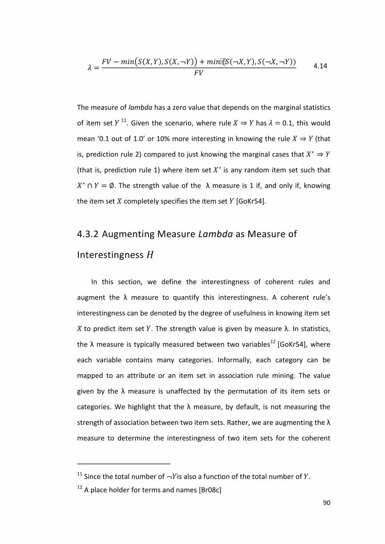
90
𝜆 =𝐹𝑉 −𝑚𝑖𝑛 𝑆 𝑋,𝑌 , 𝑆 𝑋, ¬𝑌 + 𝑚𝑖𝑛(𝑆 ¬𝑋,𝑌 , 𝑆 ¬𝑋, ¬𝑌 )
𝐹𝑉 4.14
The measure of lambda has a zero value that depends on the marginal statistics
of item set 𝑌 11. Given the scenario, where rule 𝑋 ⇒ 𝑌 has 𝜆 = 0.1, this would
mean ‘0.1 out of 1.0’ or 10% more interesting in knowing the rule 𝑋 ⇒ 𝑌 (that
is, prediction rule 2) compared to just knowing the marginal cases that 𝑋∗ ⇒ 𝑌
(that is, prediction rule 1) where item set 𝑋∗ is any random item set such that
𝑋∗ ∩ 𝑌 = ∅. The strength value of the λ measure is 1 if, and only if, knowing
the item set 𝑋 completely specifies the item set 𝑌 [GoKr54].
4.3.2 Augmenting Measure Lambda as Measure of
Interestingness 𝐻
In this section, we define the interestingness of coherent rules and
augment the λ measure to quantify this interestingness. A coherent rule’s
interestingness can be denoted by the degree of usefulness in knowing item set
𝑋 to predict item set 𝑌. The strength value is given by measure λ. In statistics,
the λ measure is typically measured between two variables12 [GoKr54], where
each variable contains many categories. Informally, each category can be
mapped to an attribute or an item set in association rule mining. The value
given by the λ measure is unaffected by the permutation of its item sets or
categories. We highlight that the λ measure, by default, is not measuring the
strength of association between two item sets. Rather, we are augmenting the λ
measure to determine the interestingness of two item sets for the coherent
11 Since the total number of ¬𝑌is also a function of the total number of 𝑌.
12 A place holder for terms and names [Br08c]

91
rules 𝑋 ∴ 𝑌. For example, the original λ measure is used to measure the
interestingness between two variables 𝐴 and 𝐵 . Let 𝐴 be an independent
variable that has two categories and let 𝐵 be a dependent variable with three
categories. The statistics of an observation on variables 𝐴 and 𝐵 are presented
in the contingency table depicted in Table 4-1,
Table 4-1: A Contingency Table for Variables A and B
𝐴1 𝐴2 Total
𝐵1 300 600 900
𝐵2 600 100 700
𝐵3 300 100 400
Total 1,200 800 2,000
Applying the formula given in [GoKr54], λ is calculated as ‘0.273’. Note,
however, that λ provides the strength of the connection between the two
variables 𝐴 and 𝐵. The strength of the relationship of the categories (or item
sets) for examples 𝐴1 ⇒ 𝐵1 and 𝐴1 ⇒ 𝐵2 are not known.
In our approach, we need to measure the strength of the relationship
between the categories rather than variables. In addition, we also need to
consider the state of presence and absence of items. Hence, we need to break
the categories further into sub-categories of existence and absence of
categories. The statistical value of these categories when applied to rule mining
can be based on the support values. Based on the data in Table 4-1, a
contingency table of all possible support values of 𝐴1, ¬𝐴1, 𝐵1 and ¬𝐵1, can be
created as depicted in Table 4-2:

92
Table 4-2: A Contingency Table for Categories 𝑨𝟏 and 𝑩𝟏
𝐴1 ¬𝐴1 Total
𝐵1 300 600 900
¬𝐵1 900 200 1,100
Total 1,200 800 2,000
The value of ¬𝐵1 for category 𝐴1 is calculated as total of 𝐴1 (or the coverage
value of 𝐴1) minus the support of 𝐵1 for category 𝐴1 (that is, 1,200 – 300 = 900).
Based on this procedure, we can construct many more contingency tables for
each possible sub category. The λ measure can now be used to quantify the
categories between 𝐴1 and 𝐵1.
Let 𝔸 and ℂ be two item sets such that 𝔸 ⊂ 𝐼 and ℂ ⊂ 𝐼. For each element
of the power-set of item set 𝔸 such that 𝑋 ∈ 𝒫(𝔸), its binary states are given
by 𝜃 such that 𝑋 = {𝜃𝑋 ,𝜃¬𝑋}. 𝜃𝑋 is the item set 𝑋 observed and 𝜃¬𝑋 is the item
set 𝑋 not observed. Similarly, 𝑌 = {𝜃𝑌 ,𝜃¬𝑌} , where 𝜃𝑌 is the item set 𝑌
observed and 𝜃¬𝑌 is the item set 𝑌 not observed. The augmented λ quantifies
the interestingness of the two item sets 𝑋 and 𝑌. Hence, we can use the
augmented λ measure to quantify interestingness of the coherent rules 𝑋 ∴ 𝑌.
It is interesting to observe that the measure of interestingness λ may have
value greater than zero even for those candidate rules that do not meet the
conditions of coherent rules. (See Appendix A for conditions of λ.) Hence, we
need to apply the coherent rules conditions to the augmented measure λ. We
call this augmented measure 𝐻. The definition of 𝐻 is given in equation 4.15:
𝐻 𝑋. .𝑌 =
𝜆, 𝑖𝑓
𝑆 𝑋,𝑌 > 𝑆 𝑋, ¬𝑌 ,𝑆 𝑋,𝑌 > 𝑆 ¬𝑋,𝑌 ,
𝑆 ¬𝑋, ¬𝑌 > 𝑆 𝑋, ¬𝑌 ,𝑆 ¬𝑋, ¬𝑌 > 𝑆 ¬𝑋,𝑌
0, 𝑜𝑡𝑒𝑟𝑤𝑖𝑠𝑒
and 4.15

93
All four conditions need to be met to give a positive value to 𝐻. The value of 𝜆
can be calculated based on the support values:
𝜆 =𝐹𝑉 − min(𝑆 𝑋,𝑌 , 𝑆 𝑋, ¬𝑌 ) − min(𝑆 ¬𝑋,𝑌 , 𝑆 ¬𝑋, ¬𝑌 )
𝐹𝑉 4.16
where:
𝐹𝑉 = min 𝑆 𝑋,𝑌 + 𝑆 𝑋, ¬𝑌 , 𝑆 ¬𝑋,𝑌 + 𝑆 ¬𝑋, ¬𝑌 4.17
The same principle is applicable to any combination of observed and non-
observed item sets such as (𝑋 and ¬𝑌), (¬𝑋 and 𝑌) and (¬𝑋 and ¬𝑌). That is,
given item sets 𝒳 = (𝑋, ¬𝑋) and item set 𝒴 = (𝑌, ¬𝑌), if the measure of
interestingness 𝐻 𝒳. .𝒴 > 0, then coherent rules 𝒳 ∴ 𝒴 are found, and its
interestingness is equal to 𝜆. This situation suggests that knowing 𝒳 will be
useful in predicting 𝒴.
Given 𝒳 ∴ 𝒴, where 𝒴 = 𝑌, the coherent rule with its interestingness can
be written as:
𝑋 ⇒ 𝑌 and ¬𝑋 ⇒ ¬𝑌, interestingness = 4.18
Similarly, a negative coherent rule having 𝒴 = 𝑌 can be written as:
𝑋 ⇒ ¬𝑌 and ¬𝑋 ⇒ 𝑌, interestingness = 4.19

94
4.3.3 The Effect of 𝐻 in the Design of the Mining
Algorithm
We highlight an important property of the coherent rules measure of
interestingness 𝐻 that pertains to the discovery of coherent rules. Coherent
rules measure of interestingness 𝐻 originated from λ which produces value as a
ratio. Each ratio value is an interval level of measurement with an arbitrary
zero. For example, the positive value given by the measure 𝐻(𝒳. .𝒴) is a ratio
over the statistics of the total number of item set 𝒴. A different denominator
value would result in a different “arbitrary zero”. Therefore, it is meaningless to
compare the same strength value across coherent rules having a different item
set 𝑌 because they are of a different scale. Analogously, it is similar to the
measure of temperature. We do not compare across the scale of Celsius and
Fahrenheit; ‘0’ Celsius is not the same as ‘0’ Fahrenheit.
Due to this above property, it is unnecessary to find all the coherent rules
with a strength value above zero but with a different item set 𝒴. Hence, once
an item set 𝑌 has been selected from 𝒴, the complexity of generating candidate
coherent rules is only bounded by the complexity of generating power-sets on
item set 𝔸 and checking the suitability of the elements in this power-set as an
antecedent to the rule 𝒳 ⇒ 𝑌.
Finding negative coherent rules is similar to finding positive coherent rules
with the difference of consequence being ¬𝑌. Hence, we can use the measure
of interestingness 𝐻 to quantify and to identify both positive and negative
coherent rules. However, since 𝑌 has a different statistic compared to ¬𝑌, the
algorithm to find all coherent rules 𝒳 ∴ 𝒴 must be a two-phase algorithm. In
this first phase, the algorithm finds positive coherent rules with 𝒳 = 𝑋 and
𝒴 = 𝑌, and negative coherent rules with 𝒳 = 𝑋 and 𝒴 = ¬𝑌 in the second
phase. Such an algorithm also allows easier separation and identification of

95
positive and negative coherent rules and has the advantage of omitting the
second phase when negative coherent rules are not required. In some
application domains, it may not be necessary to identify negative associations.
For example, in a retail situation, it would be unusual to want to know if apples
are associated with “not pears”, or if “not apples” are associated with pears.
The two-phase generation of positive and negative coherent rules thus provides
a means to generate either type of coherent rules, although both can also be
generated.
4.4 Generating Candidate Coherent Rules
In this section, we propose an approach to systematically enumerate
elements of power-set 𝔸 to avoid repetition. Recall that in transaction records,
we fix the member of item set ℂ to be a single item, and in classification
datasets, we allow the member of item set ℂ to be the class attribute value.
Assume item set 𝔸 contains a total of 𝑢 number of items {𝐼1, 𝐼2,… , 𝐼𝑢}. All
elements of power-set 𝔸 are given by item set 𝑋𝑖 where 𝑖 ∈ 2𝑢 . Assume each
item set 𝑋𝑖 is indexed using a binary system. For example, the first item set null
or item set 𝑋𝑖=1 is indexed using binary number ‘0’, item set 𝑋𝑖=2 is indexed
using ‘12’ and item set 𝑋𝑖=3 is indexed using ‘102’.
We systematically generate item set 𝑋𝑖 and pair it with a pre-selected item
set 𝑌 to form a specific candidate coherent rule 𝑋𝑖 . .𝑌 , where 1 ≤ 𝑖 ≤ 2𝑢 .
Generation of candidate coherent rules using the above order results in no
repetition. Given item set 𝔸 = {𝑎, 𝑏, 𝑐, 𝑑} and 𝑌 = {𝑒}, we show all possible
candidate coherent rules 𝑋𝑖 . .𝑌, where 𝑖 ∈ 24 starting from 𝑛𝑢𝑙𝑙. . 𝑒, in Figure
4.1:

96
Figure 4.1: Fixed-structure to represent all Candidate Coherent Rules (𝑪𝑪𝑹)
Let 𝑋. .𝑌 and 𝑋𝐸. .𝑌 be any two coherent rules such that 𝑋 ⊂ 𝑋𝐸. Employing
the order previously described enables:
(i) focus on the use of the anti-monotone [HaKa06, p. 235] property
to avoid generating and testing all 2𝑢 candidate coherent rules,
and
(ii) generation of candidate coherent rules 𝑋𝐸. .𝑌 without the need to
store all coherent rules 𝑋. .𝑌.
Following (i), candidate coherent rules 𝑋𝐸. .𝑌 are only generated after
𝑋. .𝑌. If a candidate coherent rule 𝑋. .𝑌 does not meet the anti-monotone
property, then further generation of candidate coherent rules 𝑋𝐸. .𝑌 is not
necessary (which in turn will save scanning time by not performing the tests on
coherent rules 𝑋𝐸. .𝑌 ). Consider the example depicted in Figure 4.1. If

97
candidate coherent rule 𝑑. . 𝑒 does not meet the anti-monotone property, then
𝑎𝑑. . 𝑒, 𝑏𝑑. . 𝑒 and 𝑐𝑑. . 𝑒 need not to be generated nor tested for coherent rules.
Following (ii), to generate a (current) candidate coherent rule, we only
need to know the last generated candidate coherent rule. This is because by
adding a binary number ‘12’ to the corresponding binary number of the last
generated candidate coherent rule’s antecedent item, we can obtain the
current candidate coherent rule. Hence, the memory requirement to generate a
candidate coherent rule is low. In contrast, a typical association rule mining
using the Apriori algorithm requires that all the candidates of a previous level
be kept in memory before generating all the item sets for a current level. As the
total number of item sets grows exponentially, the memory storage required
also increases. In contrast, our generation technique eliminates the need to
keep exponentially large candidate coherent rules in memory.

98
4.5 Selectively Generating the Most Effectual
Coherent Rules
The potential search space for coherent rules is large. Consequently, it is
not feasible to generate and test all the candidate coherent rules to determine
the length and strength of each. In this section, we describe a strategy to
generate the shortest coherent rules with the strongest strength values. We call
these rules the most effectual coherent rules. The algorithm we name
Generalised Shortest and Strongest Coherent Rules (𝐺𝑆𝑆_𝐶𝑅) can be used to
discover the shortest and strongest coherent rules without generating and
testing every possible combination of items.
The strategy to identify the most effectual coherent rules relies on four
constraints. These constraints inherit the anti-monotone property, and are
based on our proposed order to systematically enumerate elements of power-
set 𝔸 described in section 4.4. The process of finding the most effectual
coherent rules is conducted as an iterative process over a number of item sets.
A superset will not be generated if an item set fails to meet the conditions
posed by the constraints. In this way, generation of non-interesting candidate
coherent rules is avoided.
Among the four constraints, the constraint that is constructed based on the
properties of coherent rules in equation 3.5 is the most fundamental one. In
each iteration over a number of item sets, the four constraints are tested in a
sequential manner. The constraint in equation 3.5 is the third constraint in this
sequence. It is preceded by the first and second constraints that detect non-
interesting coherent rules based on strength values. If a candidate coherent
rule is forecast to have a strength value less than the strongest coherent rule
then this candidate coherent rule and the candidate coherent rules that have

99
associated supersets are not put forward for further consideration. The fourth
constraint ensures that the future generation of candidate coherent rules are
shorter, in term of the number of items, or at most contain the same number of
items compared to the strongest coherent rules articulated. Together, these
four constraints generate the most effectual coherent rules.
4.5.1 Finding Valid Coherent Rules
A fundamental concept of coherent rules is that the coherent rule meets all
of the conditions listed in equation 3.5 (or equation 3.6 for negative coherent
rules). In this section, we identify that some coherent rules binary conditions
inherit anti-monotone properties. These anti-monotone conditions can be
exploited to selectively test candidate coherent rules to avoid generating all
candidate coherent rules.
4.5.1.1 Changes in Support Values
In this section, we analyse the relation of the support value of 𝑋. .𝑌 and
𝑋𝐸. .𝑌 where 𝑋 ⊂ 𝑋𝐸. If support value of 𝑋𝐸 is equal or less than the support
of 𝑋, the support value is considered to possess the anti-monotone property.
Based on Table 3-4, in coherent rules mining, four support values need to
be considered for a given candidate rule 𝑋. .𝑌. Assume a function 𝑆𝑄 𝑍 (𝑋. .𝑌),
where Z = (1,2,3,4), we have four support values of a candidate coherent rule
𝑋. .𝑌:

100
(I) 𝑆𝑄1(𝑋. .𝑌) = 𝑆 𝑋,𝑌
(II) 𝑆𝑄2(𝑋. .𝑌) = 𝑆 𝑋, ¬𝑌
(III) 𝑆𝑄3(𝑋. .𝑌) = 𝑆 ¬𝑋,𝑌
(IV) 𝑆𝑄4(𝑋. .𝑌) = 𝑆 ¬𝑋, ¬𝑌
4.20
Also, let a coverage function, 𝒞(𝑋), give the frequency of occurrences of item
set 𝑋 in this transaction record. Because 𝑋 ⊂ 𝑋𝐸 and 𝑋 ∩ 𝐸 = ∅, the total
number of items contained in item set 𝑋 will be less than those contained in
item set 𝑋𝐸:
𝑋 < 𝑋𝐸 4.21
The coverage value of item set 𝑋, on the other hand, is larger or equal to this
coverage value of its superset 𝑋𝐸 in a set of transaction records:
𝒞(𝑋) ≥ 𝐶(𝑋𝐸) 4.22
Hence the coverage value has the anti-monotone property.
Recall from the contingency table shown in Table 4-2 that the coverage
value 𝐶(𝑋) is a summation of two support value functions 𝑆𝑄1 𝑋. .𝑌 and
𝑆𝑄2 𝑋. .𝑌 . Based on the same principle, other coverage values, 𝒞(¬𝑋), 𝒞(𝑌),
and 𝒞(¬𝑌), can be derived from these functions and depicted in Table 4-3:

101
Table 4-3: A Contingency Table for Candidate Coherent Rules (𝑿. .𝒀)
𝑌 ¬𝑌 Total
𝑋 𝑆𝑄1 𝑋. .𝑌 = 𝑆 𝑋,𝑌
𝑆𝑄2 𝑋. .𝑌 = 𝑆 𝑋, ¬𝑌
𝒞 𝑋
¬𝑋 𝑆𝑄3 𝑋. .𝑌 = 𝑆 ¬𝑋,𝑌
𝑆𝑄4 𝑋. .𝑌 = 𝑆 ¬𝑋, ¬𝑌
𝒞 ¬𝑋
Total 𝒞 𝑌 𝒞 ¬𝑌 𝑚
Since item set 𝑌 is pre-determined and remains unchanged throughout the
data mining process, the values given by coverage 𝒞(𝑌), and 𝒞(¬𝑌) will also
not change throughout the process. On the other hand, the value of 𝐶 𝑋 will
change because item set 𝑋 may change during the mining process. The support
value of a static item set 𝑌, 𝑆 𝑋,𝑌 , is equivalent to the support value of the
union of item set 𝑋 and a null (static) item set, plus a constant value, 𝑠𝑐:
𝑆 𝑋,𝑌 = 𝑆 𝑋,𝑛𝑢𝑙𝑙 + 𝑠𝑐 4.23
Since the union of item set 𝑋 and null is also item set 𝑋, the support value
𝑆 𝑋, 𝑛𝑢𝑙𝑙 is the coverage of 𝑋:
𝒞 𝑋 = 𝑆 𝑋,𝑛𝑢𝑙𝑙 4.24
It is therefore safe to state that the support function 𝑆 𝑋,𝑌 with an unchanged
item set 𝑌 can be mapped to coverage, and also inherits the anti-monotone
property following the property in equation 4.22:
𝑆 𝑋,𝑌 ≥ 𝑆 𝑋𝐸,𝑌 , 4.25

102
Similarly, we can reason that another support function, 𝑆 𝑋, ¬𝑌 , with a
pre-determined item set ¬𝑌 also inherits the anti-monotone property. Unlike
𝑆 𝑋,𝑌 and 𝑆 𝑋, ¬𝑌 , the other two functions: 𝑆 ¬𝑋,𝑌 and 𝑆 ¬𝑋, ¬𝑌 are
mapped to 𝒞 ¬𝑋 . 𝒞 ¬𝑋 , the additive inverse of 𝒞 𝑋 :
𝒞 𝑋 = 𝑚 − 𝒞 ¬𝑋 4.26
where 𝑚 is a fixed number of transaction records. If the coverage 𝒞 𝑋 inherits
the anti-monotone property, then 𝒞 ¬𝑋 shows the monotone property:
𝒞(¬𝑋) ≤ 𝐶(¬𝑋𝐸) 4.27
As a result, the support values 𝑆 ¬𝑋,𝑌 and 𝑆 ¬𝑋, ¬𝑌 are also monotone.
Because the support value function 𝑆𝑄1 𝑋. .𝑌 gives the support value
𝑆 𝑋,𝑌 , and the support value function 𝑆𝑄2 𝑋. .𝑌 = 𝑆 𝑋, ¬𝑌 , as in equation
4.20, we can re-write the relation between function 𝑆𝑄1 in 𝑋. .𝑌 and 𝑋𝐸. .𝑌
thus:
𝑆𝑄1 𝑋. .𝑌 ≥ 𝑆𝑄1 𝑋𝐸. .𝑌 4.28
and:
𝑆𝑄2 𝑋. .𝑌 ≥ 𝑆𝑄2 𝑋𝐸. .𝑌 4.29
Since 𝑆𝑄3 𝑋. .𝑌 = 𝑆 ¬𝑋,𝑌 and 𝑆𝑄4 𝑋. .𝑌 = 𝑆 ¬𝑋, ¬𝑌 , we write:
𝑆𝑄3 𝑋. .𝑌 ≤ 𝑆𝑄3 𝑋𝐸. .𝑌 4.30
and:
𝑆𝑄4 𝑋. .𝑌 ≤ 𝑆𝑄4 𝑋𝐸. .𝑌 4.31

103
Following equations 4.28 - 4.31, based on the anti-monotone and monotone
properties, the changes in support value functions between 𝑋𝐸. .𝑌 and 𝑋. .𝑌
are given by:
𝑆𝑄1 𝑋𝐸. .𝑌 = 𝑆𝑄1 𝑋. .𝑌 − 𝛿1 4.32
𝑆𝑄2 𝑋𝐸. .𝑌 = 𝑆𝑄2 𝑋. .𝑌 − 𝛿2 4.33
𝑆𝑄3 𝑋𝐸. .𝑌 = 𝑆𝑄3 𝑋. .𝑌 + 𝛿3 4.34
𝑆𝑄4 𝑋𝐸. .𝑌 = 𝑆𝑄4 𝑋. .𝑌 + 𝛿4 4.35
Among the four support value differences, 𝛿1 and 𝛿2 are reduced from
functions 𝑆𝑄1(𝑋. .𝑌) and 𝑆𝑄2(𝑋. .𝑌) separately due to their anti-monotone
properties. Furthermore, 𝛿3 and 𝛿4 are added to the functions 𝑆𝑄3(𝑋. .𝑌) and
𝑆𝑄4(𝑋. .𝑌) due to their monotone properties. We summarise the change in
support values using function 𝛿[𝑍]:
𝛿 𝑍 = 𝑆𝑄 𝑍 𝑋. .𝑌 − 𝑆𝑄[𝑍](𝑋𝐸. .𝑌) , where 𝑍 = 1,2,3,4 4.36
Based on the changes in support values as denoted by function 𝛿 𝑍 , we
relate each support value function between candidate coherent rules 𝑋𝐸. .𝑌
and 𝑋. .𝑌 in Table 4-4.

104
Table 4-4: A Contingency Table for Candidate Coherent Rule (𝑿𝑬. .𝒀)
𝑌 ¬𝑌 Total
𝑋𝐸 𝑆𝑄1 𝑋𝐸. .𝑌 =
𝑆𝑄1 𝑋. .𝑌 − 𝛿1
𝑆𝑄2 𝑋𝐸. .𝑌 =
𝑆𝑄2 𝑋. .𝑌 − 𝛿2
𝒞 𝑋𝐸 =
𝒞 𝑋 − (𝛿1 + 𝛿2)
¬𝑋𝐸 𝑆𝑄3 𝑋𝐸. .𝑌 =
𝑆𝑄3 𝑋. .𝑌 + 𝛿3
𝑆𝑄4 𝑋𝐸. .𝑌 =
𝑆𝑄4 𝑋. .𝑌 + 𝛿4
𝒞 ¬𝑋𝐸 =
𝒞 ¬𝑋 + (𝛿3 + 𝛿4)
Total 𝒞 𝑌 =
𝒞 𝑌 − 𝛿1 + 𝛿3
𝒞 ¬𝑌 =
𝒞 ¬𝑌 − 𝛿2 + 𝛿4
𝑚
The support value functions 𝑆𝑄 𝑍 (𝑋𝐸. .𝑌 ) and 𝑆𝑄 𝑍 (𝑋. .𝑌 ), where Z =
(1,2,3,4), are defined as:
𝑆𝑄1 𝑋𝐸. .𝑌 + 𝑆𝑄2 𝑋𝐸. .𝑌 + 𝑆𝑄3 𝑋𝐸. .𝑌 + 𝑆𝑄4 𝑋𝐸. .𝑌 =
𝑆𝑄1 𝑋. .𝑌 + 𝑆𝑄2 𝑋. .𝑌 + 𝑆𝑄3 𝑋. .𝑌 + 𝑆𝑄4 𝑋. .𝑌
+ −𝛿1 − 𝛿2 + 𝛿3 + 𝛿4
4.37
That is, we have an important relationship between the changes in the support
values (𝛿) between 𝑋𝐸. .𝑌 and 𝑋. .𝑌 viz:
𝛿1 + 𝛿2 = 𝛿3 + 𝛿4 4.38
The reduction of support values in support functions 𝑆𝑄1 𝑋. .𝑌 and
𝑆𝑄2 𝑋. .𝑌 are injected into the support functions 𝑆𝑄3 𝑋. .𝑌 and 𝑆𝑄4 𝑋. .𝑌 .
In summary, any coherent rule 𝑋𝐸. .𝑌 has a reduced (or at least) support
values on 𝑆𝑄1 𝑋𝐸. .𝑌 and 𝑆𝑄2 𝑋𝐸. .𝑌 compared to 𝑆𝑄1 𝑋. .𝑌 and
𝑆𝑄2 𝑋. .𝑌 respectively. In addition, the magnitude of the support values
reduced from 𝑆𝑄1 𝑋. .𝑌 and 𝑆𝑄2 𝑋. .𝑌 are increased on 𝑆𝑄3 𝑋. .𝑌 and
𝑆𝑄4 𝑋. .𝑌 .

105
4.5.1.2 An Anti-monotone Condition of Coherent Rules
Based on the understanding on the changes of support values, in this
section, we determine whether any of the four conditions of coherent rules in
equation 3.5 inherit the anti-monotone property.
The anti-monotone property [HaKa06, p. 235] states if a set cannot pass a
condition test, then all of its supersets will also not pass this test. In our
proposed order to generate candidate coherent rules in section 4.4, candidate
coherent rules 𝑋𝐸. .𝑌 are only generated after 𝑋. .𝑌 where 𝑋𝐸 is superset of 𝑋.
The anti-monotone property will thus be useful for pruning both ineligible
candidate coherent rules and their associated supersets.
We start with the second condition and re-write the second condition on
candidate coherent rule 𝑋. .𝑌 using support functions:
𝑆𝑄1 𝑋. .𝑌 > 𝑆𝑄3 𝑋. .𝑌 4.39
We re-write the condition as a ratio:
𝑆𝑄1 𝑋. .𝑌
𝑆𝑄3 𝑋. .𝑌 > 1 4.40
With reference to Table 4-4, the same coherent rules condition on candidate
coherent rules 𝑋𝐸. .𝑌 are:
𝑆𝑄1 𝑋𝐸. .𝑌
𝑆𝑄3 𝑋𝐸. .𝑌 > 1
𝑆𝑄1 𝑋. .𝑌 − 𝛿1
𝑆𝑄3 𝑋. .𝑌 + 𝛿3> 1
4.41
Depending on the value 𝛿1, the numerator is always smaller or equal to
𝑆𝑄1 𝑋. .𝑌 . Depending on the value 𝛿3, the denominator is larger or equal to

106
𝑆𝑄3 𝑋. .𝑌 . As a result, the ratio of the support values of candidate coherent
rules 𝑋𝐸. .𝑌 is smaller or the same as candidate coherent rules 𝑋. .𝑌. Thus, the
second condition of coherent rules in equation 4.40 inherits the anti-monotone
property.
𝑆𝑄1 𝑋. .𝑌
𝑆𝑄3 𝑋. .𝑌 ≥𝑆𝑄1 𝑋𝐸. .𝑌
𝑆𝑄3 𝑋𝐸. .𝑌 4.42
If 𝒳 ∴ 𝒴 does not satisfy the anti-monotone constraint (that is, 𝑆𝑄1 𝑋 ..𝑌
𝑆𝑄3 𝑋 ..𝑌 is
greater than ‘1’), then 𝒳ℰ ∴ 𝒴 will also not meet the constraint. Thus, we can
avoid generating 𝒳ℰ ∴ 𝒴. (A similar approach can be used to show that neither
will the first, third and fourth conditions of coherent rules inherit the anti-
monotone property. For a summary, see details in Appendix B.) By avoiding
𝒳ℰ ∴ 𝒴, we may selectively generate the needed coherent rules.
4.5.1.3 Generalising the Anti-monotone Conditions of
Coherent Rules
In this section, we extend our discussion of anti-monotone conditions over
any two pairs of two item sets regardless of their absence or presence. The
generalised anti-monotone condition is used to test all candidate coherent rules
if they are coherent rules.
Let 𝒳. .𝒴 be candidate coherent rules such that item set 𝒳 = (𝑋, ¬𝑋) and
item set 𝒴 = (𝑌, ¬𝑌). Item set 𝑋 and 𝑌 are both elements of the power-sets,
such that 𝑋 ∈ 𝒫(𝔸), 𝑌 ∈ 𝒫(ℂ), 𝑋 ≠ ∅, and 𝑌 ≠ ∅. The function 𝑆𝑄 𝑍 (𝒳. .𝒴)
finds all the support values given by 𝑆𝑄 𝑍 (𝑋. .𝑌) in equation 4.20.

107
To find coherent rules 𝒳 ∴ 𝒴 , where 𝒳 = 𝑋 and 𝒴 = 𝑌 , the function
𝑆𝑄 𝑍 (𝒳. .𝒴) finds all the support values given by 𝑆𝑄 𝑍 (𝑋. .𝑌) in equation
4.20:
(i) 𝑆𝑄1(𝒳. .𝒴) = 𝑆 𝑋,𝑌
(ii) 𝑆𝑄2(𝒳. .𝒴) = 𝑆 𝑋, ¬𝑌
(iii) 𝑆𝑄3(𝒳. .𝒴) = 𝑆 ¬𝑋,𝑌
(iv) 𝑆𝑄4(𝒳. .𝒴) = 𝑆 ¬𝑋, ¬𝑌
4.43
To find coherent rules 𝒳 ∴ 𝒴, where 𝒳 = 𝑋 and 𝒴 = ¬𝑌, the same function
𝑆𝑄 𝑍 (𝒳. .𝒴) finds all the support values:
(i) 𝑆𝑄1(𝒳. .𝒴) = 𝑆 𝑋, ¬𝑌
(ii) 𝑆𝑄2(𝒳. .𝒴) = 𝑆 𝑋,𝑌
(iii) 𝑆𝑄3(𝒳. .𝒴) = 𝑆 ¬𝑋, ¬𝑌
(iv) 𝑆𝑄4(𝒳. .𝒴) = 𝑆 ¬𝒳,𝑌
4.44
The anti-monotone constraint in equation 4.39 can be generalised over item
sets 𝒳 and 𝒴 (in either the absence or presence of item sets). That is:
𝑆𝑄1 𝒳. .𝒴 > 𝑆𝑄3 𝒳. .𝒴 4.45
The conditions 𝑆 𝑋,𝑌 > 𝑆 ¬𝑋,𝑌 and 𝑆 𝑋, ¬𝑌 > 𝑆 ¬𝑋, ¬𝑌 have the anti-
monotone property following the generalised constraint 𝑆𝑄1 𝒳. .𝒴 >
𝑆𝑄3 𝒳. .𝒴 in equation 4.45.

108
4.5.2 Finding the Strongest Coherent Rules
In section 4.5.1, we demonstrated the application of a generalised, anti-
monotone condition in order to selectively generate coherent rules. To
generate coherent rules with the strongest strength values, we imposed anti-
monotone constraints on the measure of interestingness 𝐻. This technique
enabled us to avoid generating large numbers of coherent rules and then
filtering them for the strongest coherent rules. Instead, we only generated
coherent rules that possessed the desired characteristics.
4.5.2.1 Anti-monotone Property Absence and the Measure of
Interestingness
In this section, we show that a coherent rule with strength value does not
inherit the anti-monotone property. That is, the strength value measured using
the measure of interestingness 𝐻 on 𝒳ℰ ∴ 𝒴 can be higher or lower than when
measured on 𝒳 ∴ 𝒴. In this situation, we suggest that an approximation of 𝐻
be used. The approximation should possess the anti-monotone property.
First, we will show that 𝐻 does not have the anti-monotone property. The
measure of interestingness 𝐻 stated in 4.15 can be generalised over any two
item sets 𝒳 and 𝒴 such that item set 𝒳 = (𝑋, ¬𝑋) and item set 𝒴 = (𝑌, ¬𝑌).
Item set 𝑋 and 𝑌 are both elements of the power-sets such that 𝑋 ∈ 𝒫(𝔸),
𝑌 ∈ 𝒫(ℂ), 𝑋 ≠ ∅, and 𝑌 ≠ ∅. It follows that 𝒳 ∴ 𝒴 must have positive strength
value; otherwise, it is not a coherent rule:
𝐻 𝒳 ∴ 𝒴 =
𝜆, 𝑖𝑓
𝑆𝑄1 𝒳,𝒴 > 𝑆𝑄2 𝒳,𝒴 ,
𝑆𝑄1 𝒳,𝒴 > 𝑆𝑄3 𝒳,𝒴 ,
𝑆𝑄4 𝒳,𝒴 > 𝑆𝑄2 𝒳,𝒴 ,
𝑆𝑄4 𝒳,𝒴 > 𝑆𝑄3 𝒳,𝒴
0, 𝑜𝑡𝑒𝑟𝑤𝑖𝑠𝑒
4.46

109
The 𝜆 value in 𝐻 can be calculated based on the support value functions that
give the support values in equation 4.14:
𝜆 =
𝐹𝑉 − min 𝑆𝑄1 𝒳,𝒴 , 𝑆𝑄2 𝒳,𝒴 +
min(𝑆𝑄3 𝒳,𝒴 , 𝑆𝑄4 𝒳,𝒴 )
𝐹𝑉
4.47
where:
𝐹𝑉 = 𝑚𝑖𝑛 𝑆𝑄1 𝒳,𝒴 + 𝑆𝑄2 𝒳,𝒴 , 𝑆𝑄3 𝒳,𝒴 + 𝑆𝑄4 𝒳,𝒴 4.48
𝐹𝑉 is a fixed value throughout the generation of coherent rules based on pre-
selected item set 𝑌.
The strength value of any coherent rules:
𝐻 𝒳 ∴ 𝒴 =
𝐹𝑉 − min 𝑆𝑄1 𝒳,𝒴 , 𝑆𝑄2 𝒳,𝒴 +
min(𝑆𝑄3 𝒳,𝒴 , 𝑆𝑄4 𝒳,𝒴 )
𝐹𝑉
4.49
The measure of interestingness 𝐻 for item sets 𝒳ℰ ∴ 𝒴, where 𝒳 ⊂ 𝒳ℰ has
support values based on item set 𝒳ℰ is:
𝐻 𝒳ℰ ∴ 𝒴 =
𝐹𝑉 − min 𝑆𝑄1 𝒳ℰ,𝒴 , 𝑆𝑄2 𝒳ℰ,𝒴 +
min(𝑆𝑄3 𝒳ℰ,𝒴 ,𝑆𝑄4 𝒳ℰ,𝒴 )
𝐹𝑉
4.50

110
We can re-write the function of support values between item sets 𝒳ℰ,𝒴 in
equation 4.50 using function of support values between item sets 𝒳,𝒴 based
on Table 4-4:
𝑆𝑄1 𝒳ℰ,𝒴 = 𝑆𝑄1 𝒳,𝒴 − 𝛿1 4.51
𝑆𝑄2 𝒳ℰ,𝒴 = 𝑆𝑄2 𝒳,𝒴 − 𝛿2 4.52
𝑆𝑄3 𝒳ℰ,𝒴 = 𝑆𝑄3 𝒳,𝒴 + 𝛿3 4.53
𝑆𝑄4 𝒳ℰ,𝒴 = 𝑆𝑄4 𝒳,𝒴 + 𝛿4 4.54
That is:
𝐻 𝒳ℰ ∴ 𝒴 =
𝐹𝑉 − min 𝑆𝑄1 𝒳,𝒴 − 𝛿1, 𝑆𝑄2 𝒳,𝒴 − 𝛿2 +
min(𝑆𝑄3 𝒳,𝒴 + 𝛿3, 𝑆𝑄4 𝒳,𝒴 + 𝛿4)
𝐹𝑉
4.55
Comparing 𝐻 𝒳ℰ ∴ 𝒴 in equation 4.55 to 𝐻 𝒳 ∴ 𝒴 in equation 4.49:
The minimum value of min 𝑆𝑄1 𝒳,𝒴 − 𝛿1, 𝑆𝑄2 𝒳,𝒴 − 𝛿2 can be higher
or lower than the minimum value of min(𝑆𝑄3 𝒳,𝒴 + 𝛿3, 𝑆𝑄4 𝒳,𝒴 + 𝛿4)
in equation 4.55. As a result, the strength value given by the measure of
interestingness 𝐻 𝒳ℰ ∴ 𝒴 can be higher or lower than the measure of
interestingness 𝐻 𝒳 ∴ 𝒴 . Thus, there is no anti-monotone property
associated with the measure of interestingness 𝐻.

111
4.5.2.2 Measure of Interestingness 𝐻′
We show in this section how to create the measure 𝐻′ as an approximation
of 𝐻. The measure 𝐻′ always gives a higher strength value compared to 𝐻, and
inherits the anti-monotone property. We use 𝐻’ as a means to prune away
undesirable candidate coherent rules. It is important that the approximation
suggested by 𝐻’ be at least equal or more strict than the constraint provided by
𝐻. Apart from being more strict than 𝐻, 𝐻’ needs to be designed in such a way
that it possesses the anti-monotone property.
The measure 𝐻′ is developed based on finding a maximum over three
functions, denoted by 𝐻𝑎′ , 𝐻𝑏
′ , 𝐻𝑐′ . Each mimics equation 4.49 with a difference
that is explained as follows:
Let V denote the support value given by the function 𝑆𝑄2 𝒳,𝒴 . The first
function, 𝐻𝑎′ , mimics 𝐻 except that it transfers all its support value V from
𝑆𝑄2 𝒳,𝒴 into 𝑆𝑄1 𝒳,𝒴 such that:
𝑉 = 𝑆𝑄2 𝒳,𝒴 ,
𝑆𝑄2 𝒳,𝒴 = 0 and,
𝑆𝑄1′ 𝒳,𝒴 = 𝑆𝑄1 𝒳,𝒴 + 𝑉
4.56
The new 𝑆𝑄1 𝒳,𝒴 — denoted using 𝑆𝑄1′ 𝒳,𝒴 — has support values both
from the original support function 𝑆𝑄1 𝒳,𝒴 plus 𝑉 which is the support value
of the function 𝑆𝑄2 𝒳,𝒴 , thus:
𝐻𝑎′ 𝒳 ∴ 𝒴 =
𝐹𝑉 − min 𝑆𝑄1 𝒳,𝒴 + 𝑉, 𝑆𝑄2 𝒳,𝒴 − 𝑉 +
min 𝑆𝑄3 𝒳,𝒴 , 𝑆𝑄4 𝒳,𝒴
𝐹𝑉
=𝐹𝑉 − min 𝑆𝑄3 𝒳,𝒴 ,𝑆𝑄4 𝒳,𝒴
𝐹𝑉
4.57

112
The second 𝐻𝑏′ transfers all its support values from 𝑆𝑄2 𝒳,𝒴 into 𝑆𝑄3 𝒳,𝒴
such that:
𝑉 = 𝑆𝑄2 𝒳,𝒴 ,
𝑆𝑄2 𝒳,𝒴 = 0 and,
𝑆𝑄3′ 𝒳,𝒴 = 𝑆𝑄3 𝒳,𝒴 + 𝑆𝑄2 𝒳,𝒴
4.58
The new 𝑆𝑄3 𝒳,𝒴 — denoted using 𝑆𝑄3′ 𝒳,𝒴 — has support values both
from the original support function 𝑆𝑄3 𝒳,𝒴 plus 𝑉 which is the support value
of the function 𝑆𝑄2 𝒳,𝒴 :
𝐻𝑏′ 𝒳 ∴ 𝒴 =
𝐹𝑉 − min 𝑆𝑄1 𝒳,𝒴 , 𝑆𝑄2 𝒳,𝒴 − 𝑉 +
min 𝑆𝑄3 𝒳,𝒴 + 𝑉, 𝑆𝑄4 𝒳,𝒴
𝐹𝑉
=𝐹𝑉 − min 𝑆𝑄3 𝒳,𝒴 + 𝑉, 𝑆𝑄4 𝒳,𝒴
𝐹𝑉
4.59
Finally, the third 𝐻𝑐′ transfers all its support values from 𝑆𝑄2 𝒳,𝒴 into
𝑆𝑄4 𝒳,𝒴 such that:
𝑉 = 𝑆𝑄2 𝒳,𝒴 ,
𝑆𝑄2 𝒳,𝒴 = 0 and,
𝑆𝑄4 𝒳,𝒴 = 𝑆𝑄4 𝒳,𝒴 + 𝑆𝑄2 𝒳,𝒴
4.60

113
Thus:
𝐻𝑐′ 𝒳 ∴ 𝒴
=
𝐹𝑉 − min 𝑆𝑄1 𝒳,𝒴 , 𝑆𝑄2 𝒳,𝒴 − 𝑉 +
min 𝑆𝑄3 𝒳,𝒴 , 𝑆𝑄4 𝒳,𝒴 + 𝑉
𝐹𝑉
=𝐹𝑉 − min 𝑆𝑄3 𝒳,𝒴 , 𝑆𝑄4 𝒳,𝒴 + 𝑉
𝐹𝑉
4.61
We now show that each of the output functions 𝐻𝑎′ 𝒳 ∴ 𝒴 , 𝐻𝑏
′ 𝒳 ∴ 𝒴
and 𝐻𝑐′ 𝒳 ∴ 𝒴 is at least 𝐻 𝒳 ∴ 𝒴 . As a consequence, the maximum function
𝐻′ over 𝐻𝑎′ , 𝐻𝑏
′ , and 𝐻𝑐′ will also be at least 𝐻. From equation 4.57, we know
that 𝐻 𝒳 ∴ 𝒴 is, at most, the support value of 𝐻𝑎′ 𝒳 ∴ 𝒴 :
𝐹𝑉 −𝑚𝑖𝑛 𝑆𝑄3 𝒳,𝒴 ,
𝑆𝑄4 𝒳,𝒴
𝐹𝑉 ≥
𝐹𝑉 − 𝑚𝑖𝑛 𝑆𝑄1 𝒳,𝒴 , 𝑆𝑄2 𝒳,𝒴 +
𝑚𝑖𝑛 𝑆𝑄3 𝒳,𝒴 ,𝑆𝑄4 𝒳,𝒴
𝐹𝑉
𝐻𝑎′ 𝒳 ∴ 𝒴 ≥ 𝐻 𝒳 ∴ 𝒴
4.62
From equation 4.59, we also know that 𝐻 𝒳 ∴ 𝒴 is, at most, the support value
of 𝐻𝑏′ 𝒳 ∴ 𝒴 :
𝐹𝑉 −𝑚𝑖𝑛 𝑆𝑄3 𝒳,𝒴 + 𝑉 ,
𝑆𝑄4 𝒳,𝒴
𝐹𝑉 ≥
𝐹𝑉 − 𝑚𝑖𝑛 𝑆𝑄1 𝒳,𝒴 , 𝑆𝑄2 𝒳,𝒴 +
𝑚𝑖𝑛 𝑆𝑄3 𝒳,𝒴 , 𝑆𝑄4 𝒳,𝒴
𝐹𝑉
𝐻𝑏′ 𝒳 ∴ 𝒴 ≥ 𝐻 𝒳 ∴ 𝒴
4.63

114
Lastly, from equation 4.61, we also know that 𝐻 𝒳 ∴ 𝒴 is, at most, the
support value of 𝐻𝑐′ 𝒳 ∴ 𝒴 :
𝐹𝑉 − min 𝑆𝑄3 𝒳,𝒴 ,
𝑆𝑄4 𝒳,𝒴 + 𝑉
𝐹𝑉 ≥
𝐹𝑉 − 𝑚𝑖𝑛 𝑆𝑄1 𝒳,𝒴 , 𝑆𝑄2 𝒳,𝒴 +
𝑚𝑖𝑛 𝑆𝑄3 𝒳,𝒴 , 𝑆𝑄4 𝒳,𝒴
𝐹𝑉
𝐻𝑐′ 𝒳 ∴ 𝒴 ≥ 𝐻 𝒳 ∴ 𝒴
4.64
Since 𝐻′ 𝒳 ∴ 𝒴 is the maximum function over all 𝐻𝑎′ 𝒳 ∴ 𝒴 , 𝐻𝑏
′ 𝒳 ∴ 𝒴 and
𝐻𝑐′ 𝒳 ∴ 𝒴 :
𝐻′ 𝒳 ∴ 𝒴 = 𝑚𝑎𝑥 𝐻𝑎′ 𝒳 ∴ 𝒴 ,𝐻𝑏
′ 𝒳 ∴ 𝒴 ,𝐻𝑐′ 𝒳 ∴ 𝒴 4.65
Hence, we can summarise that the interestingness measure 𝐻′ 𝒳 ∴ 𝒴 is, at
least, 𝐻 𝒳 ∴ 𝒴 :
𝐻′ 𝒳 ∴ 𝒴 ≥ 𝐻 𝒳 ∴ 𝒴 4.66
We write the measure of interestingness 𝐻′ on candidate coherent rules thus:
𝐻′ 𝒳. .𝒴 =
𝑚𝑎𝑥
𝐻𝑎′ 𝒳. .𝒴 ,
𝐻𝑏′ 𝒳. .𝒴 ,
𝐻𝑐′ 𝒳. .𝒴
, 𝑖𝑓
𝑆𝑄1 𝒳,𝒴 > 𝑆𝑄2 𝒳,𝒴 ,
𝑆𝑄1 𝒳,𝒴 > 𝑆𝑄3 𝒳,𝒴 ,
𝑆𝑄4 𝒳,𝒴 > 𝑆𝑄2 𝒳,𝒴 ,
𝑆𝑄4 𝒳,𝒴 > 𝑆𝑄3 𝒳,𝒴
0, 𝑜𝑡𝑒𝑟𝑤𝑖𝑠𝑒
4.67
We continue to show the anti-monotone property on the interestingness
measure 𝐻′ in the next section.

115
4.5.2.3 The Anti-monotone Property of the Measure of
Interestingness 𝐻′
In this section, we show the measure of interestingness 𝐻′ inheriting the
anti-monotone property. To show this, we need to show that each of the
functions 𝐻𝑎′ , 𝐻𝑏
′ , and 𝐻𝑐′ inherits the anti-monotone property.
We compare 𝐻𝑎′ 𝒳. .𝒴 based on equation 4.57 to 𝐻𝑎
′ 𝒳ℰ. .𝒴 in equation
4.68, where 𝒳 ⊂ 𝒳ℰ following Table 4-4 (or equations 4.53 & 4.54):
𝐻𝑎′ 𝒳ℰ. .𝒴 =
𝐹𝑉 −𝑚𝑖𝑛 𝑆𝑄3 𝒳ℰ,𝒴 , 𝑆𝑄4 𝒳ℰ,𝒴
𝐹𝑉
=𝐹𝑉 − 𝑚𝑖𝑛 𝑆𝑄3 𝒳,𝒴 + 𝛿3, 𝑆𝑄4 𝒳,𝒴 + 𝛿4
𝐹𝑉
4.68
𝐻𝑎′ 𝒳ℰ. .𝒴 is, at most, the support value of 𝐻𝑎
′ 𝒳. .𝒴 because
𝑚𝑖𝑛 𝑆𝑄3 𝒳,𝒴 + 𝛿3, 𝑆𝑄4 𝒳,𝒴 + 𝛿4 in equation 4.68 will be greater
than 𝑚𝑖𝑛(𝑆𝑄3 𝒳,𝒴 ,𝑆𝑄4 𝒳,𝒴 in equation 4.57:
𝐹𝑉 −𝑚𝑖𝑛 𝑆𝑄3 𝒳,𝒴 ,
𝑆𝑄4 𝒳,𝒴
𝐹𝑉 ≥
𝐹𝑉 −𝑚𝑖𝑛 𝑆𝑄3 𝒳,𝒴 + 𝛿3,
𝑆𝑄4 𝒳,𝒴 + 𝛿4
𝐹𝑉
𝐻𝑎′ 𝒳. .𝒴 ≥ 𝐻𝑎
′ 𝒳ℰ. .𝒴
4.69
If 𝒳. .𝒴 cannot meet the constraint 𝐻𝑎′ 𝒳. .𝒴 ≥ 𝑚𝑎𝑥_, where 𝑚𝑎𝑥_ is a
fixed value, then 𝒳ℰ. .𝒴 will also not meet the constraint. The function
𝐻𝑎′ 𝒳ℰ. .𝒴 inherits the anti-monotone property.

116
Similarly, we compare 𝐻𝑏′ 𝒳ℰ. .𝒴 and 𝐻𝑏
′ 𝒳. .𝒴 :
𝐹𝑉 −𝑚𝑖𝑛 𝑆𝑄3 𝒳,𝒴 + 𝑉,
𝑆𝑄4 𝒳,𝒴
𝐹𝑉 ≥
𝐹𝑉 −𝑚𝑖𝑛 𝑆𝑄3 𝒳,𝒴 + 𝛿3 + 𝑉,
𝑆𝑄4 𝒳,𝒴 + 𝛿4
𝐹𝑉
𝐻𝑏′ 𝒳. .𝒴 ≥ 𝐻𝑏
′ 𝒳ℰ. .𝒴
4.70
We also compare 𝐻𝑐′ 𝒳ℰ. .𝒴 and 𝐻𝑐
′ 𝒳. .𝒴 :
𝐹𝑉 −𝑚𝑖𝑛 𝑆𝑄3 𝒳,𝒴 ,
𝑆𝑄4 𝒳,𝒴 + 𝑉
𝐹𝑉 ≥
𝐹𝑉 −𝑚𝑖𝑛 𝑆𝑄3 𝒳,𝒴 + 𝛿3,
𝑆𝑄4 𝒳,𝒴 + 𝛿4 + 𝑉
𝐹𝑉
𝐻𝑐′ 𝒳. .𝒴 ≥ 𝐻𝑐
′ 𝒳ℰ. .𝒴
4.71
Having shown that each function 𝐻a′ 𝒳. .𝒴 , 𝐻𝑏
′ 𝒳. .𝒴 and 𝐻𝑐′ 𝒳. .𝒴 has
strength values at least the strength values given by functions 𝐻a′ 𝒳ℰ. .𝒴 ,
𝐻𝑏′ 𝒳ℰ. .𝒴 and 𝐻𝑐
′ 𝒳ℰ. .𝒴 respectively, we conclude that:
𝐻′ 𝒳. .𝒴 ≥ 𝐻′ 𝒳ℰ. .𝒴 4.72
where 𝐻′ is a maximum function over 𝐻𝑎′ , 𝐻𝑏
′ and 𝐻𝑐′ .
Assume that 𝑚𝑎𝑥_ is a fixed value. If 𝒳. .𝒴 does not meet the constraint
such that:
𝐻′ 𝒳. .𝒴 ≥ 𝑚𝑎𝑥_ 4.73
then 𝒳ℰ. .𝒴 will also not meet the constraint. This constraint is imposed using
the measure of interestingness 𝐻′ to find coherent rules with strength values of,
at least, 𝑚𝑎𝑥_; consequently, it meets the anti-monotone property. This
constraint compliments the constraint based on the condition (in contrast to
the strength value) of coherent rules in equation 4.45.

117
4.5.2.4 Another Refinement of the Measure of Interestingness
𝐻′′
𝐻’, even though it has the anti-monotone property, requires users to scan
for two support values13 in order to calculate the strength value of coherent
rules. To calculate 𝐻𝑎′ 𝒳. .𝒴 , 𝐻𝑏
′ 𝒳. .𝒴 and 𝐻𝑐′ 𝒳. .𝒴 , we need to scan for
support value functions 𝑆𝑄3 𝒳,𝒴 and 𝑆𝑄4 𝒳,𝒴 . In this section, we show a
procedure to calculate strength value 𝐻’’ using coverage values instead of
support values. A support scan requires scanning for the co-occurrence of two
item sets in a set of transaction records. In contrast, we use coverage values
that scan for the occurrence of an item set, which is less expensive in terms of
processing power hence faster. This calculation procedure produces the
measure of interestingness 𝐻’’ . The measure of interestingness 𝐻′′ has a
strength value higher than 𝐻′, and 𝐻′ has a strength value higher than 𝐻. Both
the measure of interestingness 𝐻′′ and 𝐻′ have anti-monotone properties and
can be used to avoid generating and testing all coherent rules.
The calculation of 𝐻′′ 𝒳. .𝒴 is given by the procedure below. The support
values given by the functions 𝑆𝑄3 𝒳,𝒴 and 𝑆𝑄4 𝒳,𝒴 are replaced by values
involving coverage values without scanning for the supports from transaction
records.
(i) Scan for the coverage values for the item sets 𝒳 and 𝒴; 𝒞(𝒳) and
𝒞(𝒴)
(ii) Let 𝑆𝑄1 𝒳,𝒴 = 𝒞(𝒳) and 𝑆𝑄2 𝒳,𝒴 = 0
(iii) If 𝒞(𝒳) > 𝐶(𝒴), then the support value 𝑆𝑄3 𝒳,𝒴 is replaced by
zero
13 Alternatively, we can scan for the support value of the function 𝑆𝑄1(𝒳,𝒴) and two coverage values on item set 𝒳 and 𝒴.
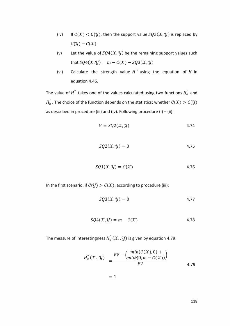
118
(iv) If 𝒞(𝒳) < 𝐶(𝒴), then the support value 𝑆𝑄3 𝒳,𝒴 is replaced by
𝒞(𝒴) − 𝒞(𝒳)
(v) Let the value of 𝑆𝑄4 𝒳,𝒴 be the remaining support values such
that 𝑆𝑄4 𝒳,𝒴 = 𝑚 − 𝒞(𝒳) − 𝑆𝑄3 𝒳,𝒴
(vi) Calculate the strength value 𝐻′′ using the equation of 𝐻 in
equation 4.46.
The value of 𝐻′′ takes one of the values calculated using two functions 𝐻𝑎′′ and
𝐻𝑏′′ . The choice of the function depends on the statistics; whether 𝒞(𝒳) > 𝐶(𝒴)
as described in procedure (iii) and (iv). Following procedure (i) – (ii):
𝑉 = 𝑆𝑄2 𝒳,𝒴 4.74
𝑆𝑄2 𝒳,𝒴 = 0 4.75
𝑆𝑄1 𝒳,𝒴 = 𝒞(𝒳) 4.76
In the first scenario, if 𝒞(𝒴) > 𝐶(𝒳), according to procedure (iii):
𝑆𝑄3 𝒳,𝒴 = 0 4.77
𝑆𝑄4 𝒳,𝒴 = 𝑚 − 𝒞(𝒳) 4.78
The measure of interestingness 𝐻𝑎′′ 𝒳. .𝒴 is given by equation 4.79:
𝐻𝑎′′ 𝒳. .𝒴
=
𝐹𝑉 − 𝑚𝑖𝑛 𝒞 𝒳 , 0 +
𝑚𝑖𝑛 0,𝑚− 𝒞(𝒳)
𝐹𝑉
= 1
4.79

119
In the second scenario, according to procedure (iv), if 𝒞(𝒴) < 𝐶(𝒳):
𝑆𝑄3 𝒳,𝒴 = 𝒞(𝒴) − 𝒞(𝒳) 4.80
𝑆𝑄4 𝒳,𝒴 = 𝑚 − 𝒞(𝒳) − (𝒞(𝒴) − 𝒞(𝒳))
= 𝑚 − 𝒞(𝒴)
= 𝒞(𝒳)
4.81
The measure of interestingness 𝐻𝑏′′ 𝒳. .𝒴 is given by equation 4.82:
𝐻𝑏′′ 𝒳. .𝒴
=𝐹𝑉 −
𝑚𝑖𝑛 𝒞 𝒳 , 0 +𝑚𝑖𝑛(𝒞(𝒴) − 𝒞(𝒳),𝑚 − 𝒞(𝒴)
𝐹𝑉
=𝐹𝑉 − 𝑚𝑖𝑛(𝒞(𝒴) − 𝒞(𝒳),𝒞(𝒳)
𝐹𝑉
4.82
The measure of interestingness of candidate coherent rules 𝐻′′ 𝒳. .𝒴 is given
by equation 4.83:
𝐻′′ 𝒳. .𝒴 = 𝑚𝑎𝑥 𝐻𝑎′′ 𝒳. .𝒴 ,𝐻𝑏
′′ 𝒳. .𝒴 4.83
We now show that 𝐻′′ is at least 𝐻′ . The measure of interestingness 𝐻′′
consists of two functions, and the measure of interestingness 𝐻′ consists of
three other functions. The first function in 𝐻′′ over candidate coherent rules is:
(i) 𝐻𝑎′′ 𝒳. .𝒴 = 1 (see equation 4.79) and thus is always higher or
the same as 𝐻′ 𝒳. .𝒴 .
The second function in 𝐻′′ 𝒳. .𝒴 is:
(ii) 𝐻𝑏′′ 𝒳. .𝒴 , which is a function over the coverage values given by
functions 𝒞(𝒴) − 𝒞(𝒳), and 𝒞(𝒳) (see equation 4.82).

120
Conversely:
(i) 𝐻𝑎′ 𝒳. .𝒴 is a function over the support values given by functions
𝑆𝑄3 𝒳,𝒴 , and 𝑆𝑄4 𝒳,𝒴 (see equation 4.57)
(ii) 𝐻𝑏′ 𝒳. .𝒴 is a function over the support values given by functions
𝑆𝑄3 𝒳,𝒴 + 𝑉, and 𝑆𝑄4 𝒳,𝒴 (see equation 4.59)
(iii) 𝐻𝑐′ 𝒳. .𝒴 is a function over the support values given by functions
𝑆𝑄3 𝒳,𝒴 , and 𝑆𝑄4 𝒳,𝒴 + 𝑉(see equation 4.61)
From Table 4-3 and under the second condition 𝒞(𝒴) < 𝐶(𝒳):
𝒞 𝒴 = 𝑆𝑄1 𝒳,𝒴 + 𝑆𝑄3 𝒳,𝒴
𝒞 𝒴 ≥ 𝑆𝑄3 𝒳,𝒴
4.84
Also:
𝒞 𝒴 = 𝑚− 𝑆𝑄2 𝒳,𝒴 − 𝑆𝑄4 𝒳,𝒴
𝒞 𝒴 ≥ 𝑆𝑄4 𝒳,𝒴
4.85
The net value of the equation 𝑚𝑖𝑛(𝒞(𝒴) − 𝒞(𝒳),𝒞(𝒳) in equation 4.82 is,
at most, 𝒞 𝒴 , which in turn must be at least 𝑆𝑄3 𝒳,𝒴 and 𝑆𝑄4 𝒳,𝒴
according to equations 4.84 and 4.85. Hence:
𝑚𝑖𝑛(𝒞 𝒴 − 𝒞 𝒳 ,𝒞 𝒳 ) ≤ 𝑚𝑖𝑛 𝑆𝑄3 𝒳,𝒴 , 𝑆𝑄4 𝒳,𝒴 4.86
𝑚𝑖𝑛(𝒞 𝒴 − 𝒞 𝒳 ,𝒞 𝒳 ) ≤ 𝑚𝑖𝑛 𝑆𝑄3 𝒳,𝒴 + 𝑉, 𝑆𝑄4 𝒳,𝒴 4.87
𝑚𝑖𝑛(𝒞 𝒴 − 𝒞 𝒳 ,𝒞 𝒳 ) ≤ 𝑚𝑖𝑛 𝑆𝑄3 𝒳,𝒴 ,𝑆𝑄4 𝒳,𝒴 + 𝑉 4.88

121
Thus:
𝐻𝑏′′ 𝒳. .𝒴 ≥ 𝐻𝑎
′ 𝒳. .𝒴
𝐻𝑏′′ 𝒳. .𝒴 ≥ 𝐻𝑏
′ 𝒳. .𝒴
𝐻𝑏′′ 𝒳. .𝒴 ≥ 𝐻𝑐
′ 𝒳. .𝒴
4.89
Since 𝐻𝑎′′ and 𝐻𝑏
′′ are higher or at least 𝐻𝑎′ ,𝐻𝑏
′ , and 𝐻𝑐′ :
𝐻′′ 𝒳. .𝒴 ≥ 𝐻′ 𝒳. .𝒴 4.90
That is, the measure of interestingness 𝐻′′ is always, at least, the measure of
interestingness 𝐻′ . If a coherent rule has a measure of interestingness 𝐻′′ less
than an expected value (say 𝑚𝑎𝑥_), then the measure of interestingness 𝐻’ or
𝐻 will also not have a strength value greater than 𝑚𝑎𝑥_ based on equation
4.90 and equation 4.66.
4.5.2.5 The Anti-monotone Property of the Measure of
Interestingness 𝐻′′
We now show the anti-monotone property of the measure of
interestingness 𝐻′′ . Equation 4.79 shows that the function 𝐻𝑎′′ 𝒳. .𝒴 and
𝐻𝑎′′ 𝒳ℰ. .𝒴 give a value of ‘1’. Based on equation 4.82, the function
𝐻𝑏′′ 𝒳ℰ. .𝒴 is written as:
𝐻𝑏′′ 𝒳ℰ. .𝒴 =
𝐹𝑉 − 𝑚𝑖𝑛(𝒞(𝒴) − 𝒞(𝒳ℰ),𝒞(𝒳ℰ) )
𝐹𝑉 4.91
According to equation 4.22:
𝒞(𝒳ℰ) ≤ 𝒞(𝒳) 4.92

122
Comparing equation 4.82 and 4.91, the equation, 𝑚𝑖𝑛(𝒞(𝒴) −
𝒞(𝒳ℰ),𝒞 𝒳ℰ ), is less or at most 𝑚𝑖𝑛(𝒞 𝒴 − 𝒞 𝒳 ,𝒞 𝒳 ); hence:
𝐻𝑏′′ 𝒳. .𝒴 ≤ 𝐻𝑏
′′ 𝒳ℰ. .𝒴 4.93
The function 𝐻𝑏′′ 𝒳ℰ. .𝒴 thus inherits anti-monotone properties. If 𝒳. .𝒴 does
not meet the constraint such as 𝐻𝑏′′ 𝒳. .𝒴 ≥ 𝑚𝑎𝑥_, where 𝑚𝑎𝑥_ is a fixed
value, then 𝒳ℰ. .𝒴 will also not meet the constraint:
𝐻′′ 𝒳. .𝒴 ≥ 𝑚𝑎𝑥_ 4.94
This implies that any constraint imposed by 𝐻′′ in equation 4.94 is less stringent
than 𝐻′ in equation 4.73.
4.5.2.6 Finding the Strongest Strength Value
In this section, we show how to use constraints imposed using 𝐻′ and 𝐻′′ in
equations 4.73 and 4.94 to find the strongest possible coherent rules.
Given a set of transaction records 𝑇, assume that item set 𝔸 contains a
total of 𝑢 items {𝐼1, 𝐼2,… , 𝐼𝑢}. All elements of power-set 𝔸 are given by item set
𝑋𝑖 where 1 ≤ 𝑖 ≤ 2𝑢 . For each item sets 𝒳 and 𝒴 , 𝒳 = (𝑋, ¬𝑋) and
𝒴 = (𝑌, ¬𝑌). Let the measure of interestingness 𝐻 𝒳. .𝒴 produce strength
value 𝑖 where1 ≤ 𝑖 ≤ 2𝑢 . The strongest coherent rules’ strength value can be
found in coherent rules with strength value 𝑖 . For some coherent rules 𝑖 , we
find the highest strength value so far is 𝑚𝑎𝑥_. We articulate all coherent rules
that meet the constraints 𝐻′′ ≥ 𝑚𝑎𝑥_, and 𝐻′ ≥ 𝑚𝑎𝑥_.

123
Over ongoing generation of candidate coherent rules, more coherent rules
can be articulated. The strongest strength value of coherent rules, 𝑚𝑎𝑥_
therefore increases. Coherent rules based on any value lower than this strength
value 𝑚𝑎𝑥_ are discarded. New coherent rules meeting the constraints are
subsequently articulated. We do not need to generate all candidate coherent
rules; rather, we selectively generate them according to the anti-monotone
properties of constraints imposed using 𝐻′ and 𝐻′′. All possible combinations
are covered without the necessity of examining all of them. As a consequence,
the coherent rules articulated will be complete while their number will depend
on the number of coherent rules available in transaction records 𝑇.
4.5.3 Finding the Shortest Coherent Rules
In this section, we formulate another constraint to find the shortest
coherent rules within transaction records. Let 𝑠𝑧 denote the number of items
contained by candidate coherent rules 𝒳. .𝒴 such that 𝑠𝑧 = |𝒳|. The shortest
coherent rules can be found over coherent rules with size 𝑠𝑧𝑖 . For these
coherent rules, we find the smallest size so far, 𝑚𝑖𝑛_𝑠𝑧. We thus articulate all
candidate coherent rules that meet the constraint:
𝑠𝑧 𝒳. .𝒴 ≤ 𝑚𝑖𝑛_𝑠𝑧 4.95
This constraint is useful to selectively generate only the shortest coherent rules.
Over a number of generations of candidate coherent rules, more coherent rules
are articulated; consequently the smallest size of candidate coherent rules,
𝑚𝑖𝑛_𝑠𝑧, reduces. Coherent rules articulated based on sizes larger than 𝑚𝑖𝑛_𝑠𝑧
are discarded. New coherent rules meeting the above constraints are
articulated. The order in which the candidate coherent rules are generated
contributes to the pruning effect of using this constraint. Candidate coherent

124
rules 𝒳. .𝒴 are typically generated in an increasing size manner. If rules 𝒳. .𝒴
do not meet the constraint, then we can avoid generating candidate coherent
rules 𝒳ℰ. .𝒴 because these also will not meet the constraint. As a result, we do
not need to generate all candidate coherent rules. Instead we selectively
generate the rules according to the anti-monotone property of constraints
imposed using the size of coherent rules. As a consequence, the coherent rules
articulated will be complete while their number will depend on the number of
coherent rules available in transaction records 𝑇.
4.5.3.1 Strategy to Discover the Most Effectual Coherent Rules
In this section we describe a strategy to mine the shortest and strongest
coherent rules. The strategy is fundamentally based on the anti-monotone
property. Four constraints are formulated to selectively generate the specific
coherent rules needed. We summarise the constraints and the support values
scan required in Table 4-5.
Table 4-5: Summary of Methods to Generate the Shortest and Strongest
Coherent Rules
No.
Anti-monotone Constraints Number of Support Values Scan
Required
References
1 𝐻′′ 𝒳. .𝒴 ≥ 𝑚𝑎𝑥_ 0; need only 2 coverage values
Section 4.5.2.5
Equations 4.94
2 𝐻′ 𝒳. .𝒴 ≥ 𝑚𝑎𝑥_ 1; 𝑆𝑄1(𝒳. .𝒴) and 2 coverage value
Section 4.5.2.3
Equations 4.73
3 𝑆𝑄1 𝒳. .𝒴 > 𝑆𝑄3 𝒳. .𝒴 1; 𝑆𝑄1(𝒳. .𝒴) and 2 coverage value
Section 4.5.1.3
Equation 4.45
4 𝑠𝑧 𝒳. .𝒴 ≤ 𝑚𝑖𝑛_𝑠𝑧 0; not applicable Section 4.5.3
Equations 4.95

125
In this strategy, we arrange the iterative use of these constraints on each
generated candidate coherent rules as:
(i) We emphasise the use of the constraints imposed on the strength
value of coherent rules in equations 4.73 and 4.94 before the use
of other constraints. They are the least expensive constraints,
especially the constraint imposed using 𝐻′′ , which uses only the
coverage values on item sets 𝒳 and 𝒴.
(ii) It follows that any candidate coherent rule that passes the
strength value constraints is checked if it also meets the condition
constraints to become a coherent rule (see equation 4.45). At this
point, any candidate coherent rule that meets all three constraints
may not be coherent rules because some may not meet the other
conditions of coherent rules.
(iii) Subsequently, a calculation of the measure of interestingness 𝐻 is
performed. If a candidate coherent rule is quantified with a
positive strength value, then it is a coherent rule. During this
calculation for real strength values, a maximum strength value
(𝑚𝑎𝑥_ ) is also maintained. Those coherent rules previously
incurred below the new 𝑚𝑎𝑥_ are removed, and
(iv) For all coherent rules with positive values discovered, we can now
articulate and maintain the minimum size of coherent rules
(𝑚𝑖𝑛_𝑠𝑧) available in the transaction records. We use the anti-
monotone constraint to prevent any future generation of
candidate coherent rules that exceed this maintained minimum
size.

126
To find the shortest coherent rules with the strongest strength value, two
variables are maintained, 𝑚𝑎𝑥_ and 𝑚𝑖𝑛_𝑠𝑧. For each candidate coherent
rules generated that meet the anti-monotone constraints, their strength value
and size 𝑠𝑧 of 𝒳 is recorded. Over a number of candidate coherent rules, the
strongest strength value is recorded in 𝑚𝑎𝑥_, and the shortest 𝒳 is recorded
in 𝑚𝑖𝑛_𝑠𝑧. Both these variables value will increase during mining. Assume a
coherent rule number 𝑟 with size 𝑠𝑧𝑟 is generated:
(i) If 𝑠𝑧𝑟 is lower than 𝑚𝑖𝑛_𝑠𝑧 discovered so far, then
𝑚𝑖𝑛_𝑠𝑧 takes the former value, and 𝑚𝑎𝑥_ takes the
strength value 𝑖 .
(ii) If 𝑠𝑧𝑟 is equal to 𝑚𝑖𝑛_𝑠𝑧 discovered so far, then 𝑚𝑎𝑥_
takes the strength value 𝑟 if it is stronger, and
(iii) If 𝑠𝑧𝑟 is higher than 𝑚𝑖𝑛_𝑠𝑧 discovered so far, then this
candidate coherent rule is not tested for its strength
value 𝑟 and is pruned.
4.96
For example, five coherent rules can be discovered from a set of transaction
records:
(i) 𝑒 ∴ {𝑔}, = 0.5
(ii) 𝑓 ∴ {𝑔}, = 0.5
(iii) 𝑎, 𝑏, 𝑐 ∴ {𝑔}, = 0.9
(iv) 𝑎, 𝑏,𝑑 ∴ {𝑔}, = 0.7, and
(v) 𝑎, 𝑏, 𝑐,𝑑 ∴ {𝑔}, = 0.6
Following our systematic enumeration of candidate coherent rules, the
candidate coherent rules are generated in a following sequence:

127
(i) 𝑎, 𝑏, 𝑐 . . {𝑔}, = 0.9
(ii) 𝑎, 𝑏,𝑑 . . {𝑔}, = 0.7
(iii) 𝑎, 𝑏, 𝑐,𝑑 . . {𝑔}, = 0.6
(iv) 𝑒 . . {𝑔}, = 0.5, and
(v) 𝑓 . . {𝑔}, = 0.5
From the first candidate coherent rule, the maximum strength value 𝑚𝑎𝑥_ =
0.9. Based on this value, the following two candidate coherent rules having the
strength values given by measure of interestingness 𝐻′ and 𝐻′′ lower than
𝑚𝑎𝑥_, are pruned. In the case that 𝐻′′ and 𝐻′ are greater than 0.9, (iii) is still
pruned by the fourth constraint because these have sizes of 𝒳 greater than the
minimum size of 3. (Note that 𝐻′′ ≥ 𝐻′ ≥ 𝐻 as in equations 4.66 and 4.90). The
minimum size of 𝒳 is recorded as 𝑚𝑖𝑛_𝑠𝑧 = 3 over the first coherent rule
found. Finally, coherent rule 𝑒 . . {𝑔} is among the shortest coherent rule.
Following the conditions set in equation 4.96, the 𝑚𝑖𝑛_𝑠𝑧 is set to ‘1’, and the
𝑚𝑎𝑥_ = 0.5. The most effectual coherent rules found are two, 𝑒 ∴ {𝑔},
= 0.5, and 𝑓 ∴ {𝑔}, = 0.5.
Following the anti-monotone property, if candidate coherent rules 𝒳. .𝒴
do not meet the anti-monotone property, the candidate coherent rules 𝒳ℰ. .𝒴
are pruned in two ways:
(i) First, if 𝑋 = 1, then we remove this item set from item set 𝔸. As
a result, no coherent rules will contain the removed item set as its
solution. The entire search space is halved. This is the most
effective way to avoid generating 𝒳ℰ. .𝒴.
(ii) Second, if 𝑋 > 1, then the algorithm avoids generating 𝒳ℰ. .𝒴,
where 𝒳 ⊂ 𝒳ℰ, and 𝒳 = 𝑋𝑖 where 1 ≤ 𝑖 ≤ 2𝑢 , and 𝑢 = 𝔸 .
The strategy prunes the search space based on the anti-monotone property and
selectively generates the most effectual coherent rules.

128
4.5.3.2 Coherent Rules Generation Algorithm (𝐺𝑆𝑆_𝐶𝑅)
In this section, we present the internal details of the algorithm –
Generalised Shortest and Strongest Coherent Rules (𝐺𝑆𝑆_𝐶𝑅) – to generate the
shortest and the strongest coherent rules from a set of transaction records. The
algorithm requires neither a minimum support threshold nor any parameters
from a user. The algorithm (𝐺𝑆𝑆_𝐶𝑅), as presented in Figure 4.2, is a recursive
algorithm that is invoked after initially setting:
(i) Candidate coherent rules 𝑅 to null.
(ii) Item set 𝔸 to the complete item set 𝐼 except those contained in
item set ℂ.
(iii) Item set 𝒴 to contain item set 𝑌 or ¬𝑌, where 𝑌 is a single item
set selected from the power set of item set ℂ.
(iv) Coverage of item set 𝒴, 𝒞(𝒴) to the total number of occurrences
on item set 𝒴.
(v) Minimum number of items on item set 𝑋 , 𝑚𝑖𝑛_𝑠𝑧 to the
cardinality of item set 𝔸.
(vi) Maximum strength value on coherent rules, 𝑚𝑎𝑥_ to zero.
(vii) Indices used to identify item set 𝑋, 𝑃𝑉𝑋1 and 𝑃𝑉𝑋2 to zero.
(viii) Index used to identify item set 𝒴, 𝑃𝑉𝒴 to the index of the item set
𝒴.
(ix) Index used to identify the last item set 𝑋, 𝑃𝑉𝑀𝑎𝑥 to the cardinality
of item set 𝔸.
(x) Transaction records 𝑇 is pointed to a set of transaction records.
(xi) Element of power-set of item set 𝔸, 𝑅𝐴 to null, and
(xii) Set of coherent rules found 𝐶𝑅 to null.

129
With reference to the algorithm in Figure 4.2, without the four constraints
in line 12, line 19, line 22, and line 23, the algorithm 𝐺𝑆𝑆_𝐶𝑅 will generate all
possible coherent rules. Line 24 will calculate the strength value of candidate
coherent rules. This finds all coherent rules in an exhaustive manner.
The introduction of line 19 is the first defence against generating candidate
coherent rules that do not have the strongest strength value. This approach
utilises the measure of interestingness 𝐻′′. This is followed by a second defence
in line 22 utilising the measure of interestingness 𝐻′. To use the latter measure
of interestingness, a scan for support values is required in line 20. Candidate
coherent rules that pass the measure of interestingness in line 19 and line 22
are further checked using the anti-monotone conditions of coherent rules,
𝑆𝑄1 𝒳,𝒴 > 𝑆𝑄3 𝒳,𝒴 , in line 23. If 𝒳. .𝒴 does not pass this third defence to
avoid generating all coherent rules, then further generations on 𝒳ℰ. .𝒴 are not
required where 𝒳 ⊂ 𝒳ℰ. Coherent rules that have passed all three defences
are then calculated for their strength value using the measure of
interestingness 𝐻. The variable of 𝑚𝑎𝑥_ is updated based on the maximum
strength value. A filter is performed to discard coherent rules that have been
articulated based on the lower value of 𝑚𝑎𝑥_ in line 29. Eventually, all
coherent rules discovered are also constrained by the shortest number of items
found in 𝒳. This fourth constraint, performed in line 12, ensures the coherent
rules found are the shortest. Although line 12 is executed prior to other three
constraints in line 19, line 22 and line 23, it is initialised by the cardinality of
item set 𝔸. All sizes of coherent rules are allowed until a coherent rule is found.
The sequence of anti-monotone constraints starts from line 19, followed by line
22, line 23 and finally line 12 (see Table 4-5).

130
Algorithm 𝑮𝑺𝑺_𝑪𝑹( candidateCoherentRules 𝑹, items 𝔸, CoverageValue 𝓒(𝓨), minimumCardinality 𝒎𝒊𝒏_𝒔𝒛, maximumStrengthValue 𝒎𝒂𝒙_𝒉, itemIndex 𝑷𝑽𝑿𝟏, itemIndex 𝑷𝑽𝑿𝟐, itemIndex 𝑷𝑽𝓨, itemIndex 𝑷𝑽𝑴𝒂𝒙, subItems 𝑻, orderedSet<index> 𝑹𝑨, RuleSet 𝑪𝑹 ) 1 //.. Initial ..// 2 If 𝑃𝑉𝑋1 > 1 3 𝑃𝑉𝑋2: = 𝑃𝑉𝑋1, 𝑃𝑉𝑋1: = 1 4 Else 5 𝑃𝑉𝑋2: = 𝑃𝑉𝑀𝑎𝑥 6 End if 7 //.. generating 𝒳. .𝒴 by enumerating item set 𝒳, where 𝒳 can be either 𝑋 or 𝑋// 8 While (𝑃𝑉𝑋1 < 𝑃𝑉𝑋2) 9 If (𝑃𝑉𝑋1! = 𝑃𝑉𝒴) AND ((𝑚𝑖𝑛_𝑠𝑧 - size of 𝑅𝐴) > 0) 10 𝑚𝑎𝑥_ = 0 11 End 12 If (𝑃𝑉𝑋1! = 𝑃𝑉𝒴) AND (size of 𝑅𝐴 ≤ 𝑚𝑖𝑛_𝑠𝑧) [ Constraint 4, See Table 4-5 ]
] 13 𝑅𝐴 concatenate(𝑃𝑉𝑋1,𝑅𝐴) 14 𝒳 {𝑖𝐿 :𝐿 ∈ 𝑅𝐴} 15 Let 𝑅 be the set of 𝒳. .𝒴, where user has determined 𝒴 to be 𝑌 or 𝑌 16 //START of Conditions for Efficient Generations// 17 Scan 𝒞 𝒳 18 Compute 𝐻′′ (𝒳,𝒴) based on coverage values 𝒞 𝒳 and 𝒞 𝒴 [ See section 4.5.2.4 ] 19 If (𝐻′′ (𝒳,𝒴) ≥ 𝑚𝑎𝑥_) [ Constraint 1, See Table 4-5]
] 20 Scan 𝑆𝑄1 𝒳,𝒴 [ See equation 4.20 ] 21 Compute 𝑆𝑄2 𝒳,𝒴 ,𝑆𝑄3 𝒳,𝒴 ,𝑆𝑄4 𝒳,𝒴 ,𝐻′(𝒳,𝒴) [ See section 4.5.2.2 ] 22 If (𝐻′(𝒳,𝒴) ≥ 𝑚𝑎𝑥_) [ See Constraint 2, Table 4-5 ]
] 23 If (𝑆𝑄1 𝒳,𝒴 > 𝑆𝑄3 𝒳,𝒴 ) [ See Constraint 3, Table 4-5 ] ] 24 ∀𝑟 ∈ 𝑅 compute 𝑟 based on 𝐻(𝒳,𝒴), compute 𝑠𝑧𝑟 and store it
25 Update 𝑚𝑖𝑛_𝑠𝑧 over the shortest 𝑠𝑧𝑟 found 26 Update 𝑚𝑎𝑥_ based on the strongest 𝑟 found 27 If (𝑟 ≥ 𝑚𝑎𝑥_) [ Store and Filter unnecessary CRs ] 28 𝐶𝑅 = 𝐶𝑅 ∪ 𝑅 29 𝑡𝑜𝐹𝑖𝑙𝑡𝑒𝑟={ 𝑐𝑟: 𝑐𝑟 ∈ 𝐶𝑅 and 𝑐𝑟 < 𝑚𝑎𝑥_ and 𝑠𝑧𝑐𝑟 > 𝑚𝑖𝑛_𝑠𝑧 } 30 𝐶𝑅 = 𝐶𝑅 − 𝑡𝑜𝐹𝑖𝑙𝑡𝑒𝑟 31 End 32 If (𝑃𝑉𝑋1 > 1) 33 𝑅𝐴 concatenate(𝑃𝑉𝑋1 ,𝑅𝐴) 34 (𝑅,𝔸,𝒞 𝒴 ,𝑚𝑖𝑛_𝑠𝑧,𝑚𝑎𝑥_,𝑃𝑉𝑋1,𝑃𝑉𝑋2 ,𝑃𝑉𝒴,𝑃𝑉𝑀𝑎𝑥 ,𝑅𝐴,𝐶𝑅) =
𝐺𝑆𝑆_𝐶𝑅 (𝑅,𝔸,𝒞 𝒴 ,𝑚𝑖𝑛_𝑠𝑧,𝑚𝑎𝑥_,𝑃𝑉𝑋1 ,𝑃𝑉𝑋2 ,𝑃𝑉𝒴,𝑃𝑉𝑀𝑎𝑥 ,𝑅𝐴,𝐶𝑅) 35 𝑅𝐴 (𝑅𝐴− 𝑃𝑉𝑋1) //remove an item from the buffer of item set 𝒳// 36 End 37 Else 38 𝑖𝑡𝑒𝑚𝑇𝑜𝑅𝑒𝑚𝑜𝑣𝑒 = {X: X is the item set of some 𝑟 ∈ 𝑅 and 𝑋 = 1 } 39 𝔸 = 𝔸 − 𝑖𝑡𝑒𝑚𝑇𝑜𝑅𝑒𝑚𝑜𝑣𝑒 40 End 41 Else 42 𝑖𝑡𝑒𝑚𝑇𝑜𝑅𝑒𝑚𝑜𝑣𝑒 = {X: X is the item set of some 𝑟 ∈ 𝑅 and 𝑋 = 1 } 43 𝔸 = 𝔸 − 𝑖𝑡𝑒𝑚𝑇𝑜𝑅𝑒𝑚𝑜𝑣𝑒

131
44 End 45 Else 46 𝑖𝑡𝑒𝑚𝑇𝑜𝑅𝑒𝑚𝑜𝑣𝑒 = {X: X is the item set of some 𝑟 ∈ 𝑅 and 𝑋 = 1 } 47 𝔸 = 𝔸 − 𝑖𝑡𝑒𝑚𝑇𝑜𝑅𝑒𝑚𝑜𝑣𝑒 48 End 49 //End of Conditions for Efficient Generations// 50 End 51 𝑃𝑉𝑋1 ≔ 𝑃𝑉𝑋1 + 1 //increase the item index// 52 End
Figure 4.2: Shortest and Strongest Coherent Rules Generation Algorithm
(𝑮𝑺𝑺_𝑪𝑹)
Following the anti-monotone property, if candidate coherent rules 𝒳. .𝒴
do not meet the anti-monotone property, algorithm 𝐺𝑆𝑆_𝐶𝑅 avoids generating
coherent rules 𝒳ℰ. .𝒴 in two ways:
(i) First, if 𝒳 = 1, then we remove this item set from item set 𝔸 in
line 37, line 41 and line 45. As a result, no coherent rule will
contain the removed item set as its solution. The entire search
space is halved.
(ii) Second, if 𝒳 > 1, then the algorithm avoids generating 𝒳ℰ. .𝒴
by not entering into a recursion in line 34 (for example, if a
condition in any of the line 12, line 19, line 22 and line 23 is not
met, line 34 is skipped). Hence, all 𝒳ℰ. .𝒴 are not generated after
𝒳. .𝒴 , where 𝒳 ⊂ 𝒳ℰ , and 𝒳 = 𝑋𝑖 where 1 ≤ 𝑖 ≤ 2𝑢 , and
𝑢 = 𝔸 .
The entire algorithm terminates when all elements of power-set in item set 𝔸
are considered. 𝑃𝑉𝑋1 will increase value due to line 51 and 𝑃𝑉𝑋1 equals 𝑃𝑉𝑋2. As
a result, the program terminates due to the condition in line 8.
132
4.6 An Extended Coherent Rules Generation
Algorithm
In business, there will be cases where longer coherent rules with arbitrarily
strength values are sought [SiInSr08a]. In this section, we extend algorithm
𝐺𝑆𝑆_𝐶𝑅 to also generate these coherent rules. The new algorithm, called the
Extended Shortest and Strongest Coherent Rules (𝐸𝑆𝑆_𝐶𝑅), is able to generate
all coherent rules generated by the algorithm 𝐺𝑆𝑆_𝐶𝑅. In addition, it allows the
discovery of coherent rules:
(i) all available sizes, and
(ii) all available strength values.
The algorithm 𝐸𝑆𝑆_𝐶𝑅 allows users to communicate their requirements via two
parameters 𝐿 and 𝑊, where the constraints imposed on the number of items,
and the strength values allowed in coherent rules, are relaxed. The generation
of coherent rules with relaxed constraints often results in many more coherent
rules. These will include coherent rules that have weaker strength values and a
lengthy item set 𝒳. Nonetheless, the choice – longer or shorter, stronger or
weaker – belongs to the user. The salient features of the original algorithm
𝐺𝑆𝑆_𝐶𝑅 are kept in that the extended algorithm does not require the user to
specify a minimum strength value or the number of items needed.
4.6.1 Strength Value Window (𝑊)
In this section, we show how to find coherent rules other than those with
the strongest strength value.
Given a set of transaction records 𝑇, assume that item set 𝔸 contains a
total of 𝑢 items {𝐼1, 𝐼2,… , 𝐼𝑢}. All elements of power-set 𝔸 are given by item set

133
𝑋𝑖 where 1 ≤ 𝑟 ≤ 2𝑢 . For each item sets 𝒳 and 𝒴, where 𝒳 = (𝑋, ¬𝑋) and
𝒴 = (𝑌,𝑌), let the measure of interestingness 𝐻 𝒳. .𝒴 produce strength
value 𝑟 where 1 ≤ 𝑟 ≤ 2𝑢 . The strongest coherent rules strength value can be
found over coherent rules with strength value 𝑟 . Let 𝑚𝑎𝑥_ be the strongest
strength value that can be discovered in 𝑇, and let 𝑚𝑖𝑛_ be the lowest
strength value allowed to be discovered. Depending on the strongest strength
value available in 𝑇 , 𝑚𝑖𝑛_ is a function over 𝑚𝑎𝑥_ and strength value
window (𝑊):
𝑚𝑖𝑛_ = 𝑚𝑎𝑥_ × (1 −𝑊) 4.97
In the case that a user needs all the strongest coherent rules, then 𝑊is left at its
default ‘0’. In the case that a user needs all coherent rules at an arbitrary
strength value, then 𝑊 is set at 1. By setting 𝑊 = 1, the generation of coherent
rules is free from the constraints imposed using 𝐻′′, and 𝐻′. The algorithm will
generate coherent rules based on the anti-monotone condition of coherent
rules in equation 4.45. The use of the parameter 𝑊can be differentiated from
the use of a minimum support threshold because the user does not need to
know the lowest strength value 𝑚𝑖𝑛_ nor the value of 𝑚𝑎𝑥_.
4.6.2 Length Window (𝐿)
In this section, we show how to find coherent rules other than the shortest
rules. Let 𝑚𝑖𝑛_𝑠𝑧 denote the minimum number of items found over coherent
rules 𝒳 ∴ 𝒴. Let 𝑚𝑎𝑥_𝑠𝑧 denote the maximum number of items allowed to be
discovered. The user specifies the parameter 𝐿 to increase the size of coherent
rules found, such that:

134
𝑚𝑎𝑥_𝑠𝑧 = 𝑚𝑖𝑛_𝑠𝑧 + 𝐿 4.98
A user does not need to know the shortest or the longest coherent rules that
can be found from a set of transaction records. In the case that a user needs all
the shortest coherent rules, then 𝐿 is left at its default ‘0’. In the case that a
user needs all sizes of coherent rules, then 𝐿 is set to its maximum of 𝔸 . This
inclusion of 𝐿 relaxes and generalises the use of constraint that would
otherwise use 𝑚𝑖𝑛_𝑠𝑧 to find only the minimum sizes of coherent rules
discovered through 𝐺𝑆𝑆_𝐶𝑅.
4.6.3 The Algorithm 𝐸𝑆𝑆_𝐶𝑅
The algorithm 𝐸𝑆𝑆_𝐶𝑅 generalises the results produced using algorithm
𝐺𝑆𝑆_𝐶𝑅, and is able to produce a greater number of coherent rules. It uses two
additional parameters to control and allow the generation of more relaxed
coherent rules.
An additional number of items (𝐿) is added to the minimum number of
items found, 𝑚𝑖𝑛_𝑠𝑧. All coherent rules, which are 𝒳 at most or below
𝑚𝑖𝑛_𝑠𝑧 + 𝐿, are now considered as 𝑚𝑎𝑥_𝑠𝑧. The parameter 𝑊 (specified by
the user) further lowers the maximum strength value (𝑚𝑎𝑥_) discovered. This
new variable is called 𝑚𝑖𝑛_. These adjustment are made into the algorithm
𝐺𝑆𝑆_𝐶𝑅. Fundamentally, the changes are in line 25 and 26 in Figure 4.3. Both
parameters 𝐿 and 𝑊 are considered for the new variables 𝑚𝑎𝑥_𝑠𝑧 and
𝑚𝑖𝑛_ as stated in equations 4.97 and 4.98. The use of these new variables
causes the following alteration:
(i) All variables 𝑚𝑖𝑛_𝑠𝑧 are replaced by 𝑚𝑎𝑥_𝑠𝑧 in lines 9, 12, 25, 29,
and 34.

135
(ii) All variables 𝑚𝑎𝑥_ are replaced by 𝑚𝑖𝑛_ in lines 10, 19, 22, 26,
27, 29 and 34.
It is also important to set 𝑚𝑖𝑛_ to zero in line 10 if the difference between the
current size 𝒳 and the 𝑚𝑎𝑥_𝑠𝑧 is greater than the allowed additional size 𝐿. By
setting the 𝑚𝑖𝑛_ to zero, 𝐸𝑆𝑆_𝐶𝑅 searches for the strongest strength values
among shorter coherent rules without being entrapped into longer coherent
rules with stronger strength. That is, within the allowed sizes between 𝑚𝑖𝑛_𝑠𝑧
and 𝑚𝑎𝑥_𝑠𝑧, the optimal strength value is sought on 𝑚𝑎𝑥_. Based on this
optimal strength value and the window strength value 𝑊 , the minimum
allowed strength value is calculated as 𝑚𝑖𝑛_. For candidate coherent rules
with sizes below 𝑚𝑖𝑛_𝑠𝑧, a new positive strength value is recorded via setting
𝑚𝑖𝑛_ = 0. Otherwise, candidate coherent rules with sizes above 𝑚𝑎𝑥_𝑠𝑧 are
pruned.

136
Algorithm 𝑬𝑺𝑺_𝑪𝑹( candidateCoherentRules 𝑹, items 𝔸, CoverageValue 𝓒(𝓨), extraCardinalityAllowed 𝑳, extraStrengthValueAllowed 𝑾, maximumCardinality 𝒎𝒂𝒙_𝒔𝒛, minimumStrengthValue 𝒎𝒊𝒏_𝒉, itemIndex 𝑷𝑽𝑿𝟏, itemIndex 𝑷𝑽𝑿𝟐, itemIndex 𝑷𝑽𝓨, itemIndex 𝑷𝑽𝑴𝒂𝒙, subItems 𝑻, orderedSet<index> 𝑹𝑨, RuleSet 𝑪𝑹 ) 1 //.. Initial ..// 2 If 𝑃𝑉𝑋1 > 1 3 𝑃𝑉𝑋2: = 𝑃𝑉𝑋1, 𝑃𝑉𝑋1: = 1 4 Else 5 𝑃𝑉𝑋2: = 𝑃𝑉𝑀𝑎𝑥 6 End if 7 //.. generating 𝒳. .𝒴 by enumerating item set 𝒳, where 𝒳 can be either 𝑋 or 𝑋// 8 While (𝑃𝑉𝑋1 < 𝑃𝑉𝑋2) 9 If (𝑃𝑉𝑋1! = 𝑃𝑉𝒴) AND ((𝑚𝑎𝑥_𝑠𝑧 - size of 𝑅𝐴 ) > 𝐿) 10 𝑚𝑖𝑛_ = 0 11 End 12 If (𝑃𝑉𝑋1! = 𝑃𝑉𝒴) AND (size of 𝑅𝐴 ≤ 𝑚𝑎𝑥_𝑠𝑧)
] 13 𝑅𝐴 concatenate(𝑃𝑉𝑋1,𝑅𝐴) 14 𝒳 {𝑖𝐿 :𝐿 ∈ 𝑅𝐴} 15 Let 𝑅 be the set of 𝒳. .𝒴, where user has determined 𝒴 to be 𝑌 or 𝑌 16 //START of Conditions for Efficient Generations// 17 Scan 𝒞 𝒳 18 Compute 𝐻′′ (𝒳,𝒴) based on coverage values 𝒞 𝒳 and 𝒞 𝒴 19 If (𝐻′′ (𝒳,𝒴) ≥ 𝑚𝑖𝑛_)
] 20 Scan 𝑆𝑄1 𝒳,𝒴 21 Compute 𝑆𝑄2 𝒳,𝒴 ,𝑆𝑄3 𝒳,𝒴 ,𝑆𝑄4 𝒳,𝒴 ,𝐻′(𝒳,𝒴) 22 If (𝐻′(𝒳,𝒴) ≥ 𝑚𝑖𝑛_) Table 4-5.
Table 4-5] 23 If (𝑆𝑄1 𝒳,𝒴 > 𝑆𝑄3 𝒳,𝒴 ) Table 4-5.
Table 4-5]
24 ∀𝑟 ∈ 𝑅 compute 𝑟 based on 𝐻(𝒳,𝒴), compute 𝑠𝑧𝑟 and store it 25 Update 𝑚𝑎𝑥_𝑠𝑧 based on the shortest 𝑠𝑧𝑟 found and 𝐿 [ see equation 4.98 ] 26 Update 𝑚𝑖𝑛_ over the strongest 𝑟 found and 𝑊 [ see equation 4.97 ] 27 If (𝑟 ≥ 𝑚𝑖𝑛_) 28 𝐶𝑅 = 𝐶𝑅 ∪ 𝑅 29 𝑡𝑜𝐹𝑖𝑙𝑡𝑒𝑟={𝑐𝑟: 𝑐𝑟 ∈ 𝐶𝑅 and 𝑐𝑟 < 𝑚𝑖𝑛_ and 𝑠𝑧𝑐𝑟 > 𝑚𝑎𝑥_𝑠𝑧 } 30 𝐶𝑅 = 𝐶𝑅 − 𝑡𝑜𝐹𝑖𝑙𝑡𝑒𝑟 31 End 32 If (𝑃𝑉𝑋1 > 1) 33 𝑅𝐴 concatenate(𝑃𝑉𝑋1 ,𝑅𝐴) 34 (𝑅,𝔸,𝒞 𝒴 ,𝑚𝑎𝑥_𝑠𝑧,𝑚𝑖𝑛_,𝑃𝑉𝑋1,𝑃𝑉𝑋2 ,𝑃𝑉𝒴,𝑃𝑉𝑀𝑎𝑥 ,𝑅𝐴,𝐶𝑅) =
𝐸𝑆𝑆_𝐶𝑅 (𝑅,𝔸,𝒞 𝒴 ,𝑚𝑎𝑥_𝑠𝑧,𝑚𝑖𝑛_,𝑃𝑉𝑋1,𝑃𝑉𝑋2 ,𝑃𝑉𝒴,𝑃𝑉𝑀𝑎𝑥 ,𝑅𝐴,𝐶𝑅) 35 𝑅𝐴 (𝑅𝐴− 𝑃𝑉𝑋1) //remove an item from the buffer of item set 𝒳// 36 End 37 Else 38 𝑖𝑡𝑒𝑚𝑇𝑜𝑅𝑒𝑚𝑜𝑣𝑒 = {X: X is the item set of some 𝑟 ∈ 𝑅 and 𝑋 = 1 } 39 𝔸 = 𝔸 − 𝑖𝑡𝑒𝑚𝑇𝑜𝑅𝑒𝑚𝑜𝑣𝑒 40 End 41 Else 42 𝑖𝑡𝑒𝑚𝑇𝑜𝑅𝑒𝑚𝑜𝑣𝑒 = {X: X is the item set of some 𝑟 ∈ 𝑅 and 𝑋 = 1 }

137
43 𝔸 = 𝔸 − 𝑖𝑡𝑒𝑚𝑇𝑜𝑅𝑒𝑚𝑜𝑣𝑒 44 End 45 Else 46 𝑖𝑡𝑒𝑚𝑇𝑜𝑅𝑒𝑚𝑜𝑣𝑒 = {X: X is the item set of some 𝑟 ∈ 𝑅 and 𝑋 = 1 } 47 𝔸 = 𝔸 − 𝑖𝑡𝑒𝑚𝑇𝑜𝑅𝑒𝑚𝑜𝑣𝑒 48 End 49 //End of Conditions for Efficient Generations// 50 End 51 𝑃𝑉𝑋1 ≔ 𝑃𝑉𝑋1 + 1 //increase the item index// 52 End
Figure 4.3: Extended Shortest and Strongest Coherent Rules Generation
Algorithm (𝑬𝑺𝑺_𝑪𝑹)
At any value of 𝐿 and 𝑊, the algorithm 𝐸𝑆𝑆_𝐶𝑅 generates the complete set
of required coherent rules. In the first phase, the item set 𝒴 is per-determined
to contain an item set 𝑌, and ¬𝑌 in the second phase, where 𝑌 is an item
chosen from all items contained in the transaction records. Positive coherent
rules are discovered from the first phase:
𝑋 ⇒ 𝑌 and ¬𝑋 ⇒ ¬𝑌 4.99
Negative coherent rules are discovered from the second phase:
𝑋 ⇒ ¬𝑌 and ¬𝑋 ⇒ 𝑌 4.100
By repeating the coherent rules algorithm 𝐸𝑆𝑆_𝐶𝑅 twice using different 𝒴, we
can find both positive and negative coherent rules.
4.7 Conclusion
In this chapter, we have devised a measure for coherent rules based on the
classic statistics of lambda. The measure provides coherent rules with a
quantified strength value for their interestingness. A positive strength value on

138
coherent rules indicates that each coherent rule has a prediction ability
stronger than the marginal probability on the consequence item set.
We devised a strategy to find the most effectual set of coherent rules.
‘Effectual’ refers to those coherent rules that have the strongest strength value
and contain the least number of items in the rule. We consider that the shortest
rules with the strongest strength values are more actionable than long rules.
We then devised an algorithm (called Generalised Shortest and Strongest
Coherent Rules (𝐺𝑆𝑆_𝐶𝑅)) for the generation of coherent rules. This algorithm
does not take any parameter values. However, the algorithm is flexible; it can
find rules that are weaker and longer if these are desired by the user. In this
situation, the user needs to supply L as an additional number of items on top of
the shortest coherent rules that can be discovered, and W%, which is a
tolerance percentage from the strongest strength value that can be found in a
given set of transaction records. This extended algorithm is called Extended
Shortest and Strongest Coherent Rules (𝐸𝑆𝑆_𝐶𝑅). The parameter values L and
W% do not require the user to have background knowledge of minimum
support thresholds, strength values or the size of rules in a given dataset.
Hence, our algorithm does not pose the problem associated with the 𝐴𝑝𝑟𝑖𝑜𝑟𝑖
algorithm. In addition, the design of our algorithm minimises the amount of
memory usage during the rule generation process, and selectively generates
coherent rules by exploiting the anti-monotone property of coherent rules, the
measure of interestingness and the size of coherent rules. Furthermore,
coherent rules found can be decoupled to obtain association rules.
In this chapter we have demonstrated how the algorithm 𝐸𝑆𝑆_𝐶𝑅
discovers the complete set of coherent rules needed by a user. The next
chapter presents an evaluation of this extended algorithm.

139
Chapter 5
ANALYSIS OF
PERFORMANCE
5.1 Introduction
In Chapter 3, we presented a coherent rules (CR) mining framework. This
framework identifies the associations between item sets without the need to
specify a minimum support threshold. The rules identified were pseudo-
implications of equivalences. That is, they can be mapped to logical
equivalences of propositional logic. The implementation of the CR mining
framework requires handling the exponential large search space. In Chapter 4,
we devised a strategy to find the complete set of coherent rules from a set of
transaction records. The strategy identified four constraints based on the anti-
monotone property. We realised and generalised the strategy with the
algorithm 𝐸𝑆𝑆_𝐶𝑅 to discover coherent rules of arbitrary minimum sizes and
strength values. The algorithm, when it has default parameter values of 𝐿 = 0
and 𝑊 = 0, selectively generates the shortest and strongest coherent rules.
In this chapter, we perform a series of experiments on a standard dataset
used by researchers known as Zoo [Fo90]. We also use a number of basket
datasets (BMS-View1, BMS-View2, BMS-Pos [KoBrFrMaZh00] and Retail

140
[BrSwVaWe99]) supplied by various retail supermarket stores. Four facets of
the algorithm 𝐸𝑆𝑆_𝐶𝑅 are tested. First, we test the effectiveness of each
constraint in 𝐸𝑆𝑆_𝐶𝑅 in limiting the search space. An effective constraint will
preclude generation of non-interesting rules at an early stage of pruning and
thus prevent the resource wastage incurred where more than one constraint
may be applied. Any non-interesting rule that is not avoided will be considered
residual.
Second, we test the quality of rules mined by this proposed algorithm.
Coherent rules mined using 𝐸𝑆𝑆_𝐶𝑅 are decoupled into association rules. These
rules are compared with association rules discovered using the classic
association rule mining algorithm, 𝐴𝑝𝑟𝑖𝑜𝑟𝑖 [AgSr94]. 𝐴𝑝𝑟𝑖𝑜𝑟𝑖 is based on the
support and confidence framework, and is known to represent a number of
other algorithms that are based on the same mining framework
[WuKuQuGhYaMoMcNgLiYuZhStHaSt07]. By comparing the association rules
discovered via 𝐸𝑆𝑆_𝐶𝑅 and 𝐴𝑝𝑟𝑖𝑜𝑟𝑖, we expect to conclude that 𝐸𝑆𝑆_𝐶𝑅 can
discover association rules with (i) low support, (ii) high support and (iii) absence
of items. On the other hand, 𝐴𝑝𝑟𝑖𝑜𝑟𝑖 finds association rules above a minimum
support threshold.
Third, we test the efficiency of 𝐸𝑆𝑆_𝐶𝑅 with respect to increasing
parameter values of 𝐿 and 𝑊 and a unique number of attribute values available
in a dataset. Theoretically, as the parameter values of 𝐿 and 𝑊 increase, longer
rules with lower strength values will be discovered. Lastly, we test 𝐸𝑆𝑆_𝐶𝑅 for
its efficiency in discovering coherent rules in real-world and large retail
transactional datasets to determine the practicality of the proposed algorithm.
This chapter is divided into five sections. In section 5.2, we introduce the
Zoo dataset, which we used for performance evaluation. In section 5.3, we test
the goodness of constraints used in the algorithm 𝐸𝑆𝑆_𝐶𝑅. The quality of rules

141
in terms of finding interesting association rules with low and high support
values, and absence of items, is tested in section 5.4. This section concludes
with a list of distinct features observed in the algorithm 𝐸𝑆𝑆_𝐶𝑅. In section 5.5,
we test the performance of 𝐸𝑆𝑆_𝐶𝑅 under gradually relaxed constraints. The
number of coherent rules, discovery time as the parameter values 𝐿, 𝑊 and the
number of attribute values (in dataset) increase are all recorded. In section 5.6,
using four real-world and large retail transactional datasets, we investigate the
number and size of rules that can be discovered. We conclude this chapter in
section 5.7.
5.2 Preliminaries
5.2.1 Zoo Dataset
We use the Zoo dataset [Fo90] to perform a series of experiments before
using real-world transaction records to test the usability of 𝐸𝑆𝑆_𝐶𝑅 for Market
Basket Analysis. A detailed description of the Zoo dataset can be found in
Appendix C. The Zoo dataset contains a collection of animal characteristics and
their classes in a Zoo. This dataset was chosen because the characteristics of
animals are well understood. The small size of this dataset facilitates the
interpretation of findings. As a result, the interestingness of found rules can be
compared and contrasted based on general understanding. We summarise the
statistics on this Zoo dataset in Table 5-1.

142
Table 5-1: Summary of the Statistics for the Zoo Dataset
Total Number of Attributes 23
(16 attributes and 7 class attributes)
Total Attribute Values 21
(15 binary values and 1 multi-value attribute)
Total Class Values 7
(7 binary values)
Total Instances 101
Number of Attribute Values
per Instance
16
The Zoo dataset has seven classes of animals. It has a spectrum of
frequency of occurrences in the transaction records. We show the frequencies
of each class in Table 5-2. If the frequency of occurrence is below 5%, we
consider the class of animal to be rare. Otherwise, the class is identified as
frequent (that is, incurring at least 5% of support values).
Table 5-2: Total Frequency of Class Attributes
No. Class Attributes
Frequency of
Occurrence
Percentage
(%)
Type of Association
1 reptile 5/101 4.95 Infrequent
2 mammal 41/101 40.59 Frequent
3 invertebrate 10/101 9.90 Frequent
4 insect 8/101 7.92 Frequent
5 fish 13/101 12.87 Frequent
6 bird 20/101 19.80 Frequent
7 amphibian 4/101 3.96 Infrequent
From Table 5-2, five class attributes have a frequency of occurrence of at least
more than 5%. These are mammal, invertebrate, insect, fish, and bird. The class

143
mammal is most frequently observed, followed by bird and fish. On the other
hand, the class amphibian and class reptile are the least observed at 3.96% and
4.95% respectively.
5.3 Goodness of Constraints
5.3.1 Evaluation Measures
In this section, we investigate the usefulness of constraints introduced in
section 4.5.1.3, 4.5.2.3, 4.5.2.5 and 4.5.3 (summarised in Table 4-5 in section
4.5.3.1) that can be used to limit the search space by precluding the generation
of candidate coherent rules that cannot lead to coherent rules. The residual of a
constraint is defined as the total number of candidate coherent rules allowed
by a constraint less the actual number of coherent rules found for a class.
Letting 𝐶𝐶𝑅 be the total number of candidate coherent rules allowed, and
letting 𝐶𝑅 be the number of coherent rules discovered, then the residual ( 𝑅 )
is given by:
𝑅 = 𝐶𝐶𝑅 − 𝐶𝑅 5.1
The residual can be expressed as a percentage:
𝑅 (%) = 𝐶𝐶𝑅 − 𝐶𝑅
𝐶𝐶𝑅 5.2
The lower the value of 𝑅%, the more the goodness of having the constraint
increases. Nonetheless, the 𝐶𝐶𝑅 on each constraint cannot be measured
directly by embedding a counter after each constraint. This is because each

144
generated candidate coherent rule is tested using all four constraints. The effect
of one constraint flows onto others in both current and following iterations. The
𝐸𝑆𝑆_𝐶𝑅 algorithm uses four constraints (refer to Table 4-5) in a sequential
manner for each generated candidate coherent rule, as follows:
(i) 𝐶1: 𝐻′′ ≤ 𝑚𝑖𝑛_
(ii) 𝐶2: 𝐻′ ≤ 𝑚𝑖𝑛_
(iii) 𝐶3: 𝑆𝑄1 𝒳. .𝒴 > 𝑆𝑄3 𝒳. .𝒴
(iv) 𝐶4: 𝑠𝑧 𝒳. .𝒴 ≤ 𝑚𝑎𝑥_𝑠𝑧
In this chapter, we demonstrate the cumulative effect of each individual
constraint. That is, the number of candidate coherent rules recorded after using
the second constraint is not only affected by the first constraint in a current
iteration but also affected by the third in a previous iteration. For example,
assume coherent rules are discovered from a set of transaction records that
contains the item set {a,b,c,d}. The generation of a candidate coherent rule pair
{𝑎, 𝑏}. . {𝑑} at strength value 𝐻′′ is only possible if {𝑎}. . {𝑑} has been allowed by
the third constraint in a previous iteration. As a result, {𝑎, 𝑏}. . {𝑑} is allowed
through constraints as a cumulative effect.
Fundamentally, 𝐸𝑆𝑆_𝐶𝑅 must use the constraint 𝐶3 on each candidate
coherent rule pair generated. This will prevent the number of tested candidate
coherent rules from increasing. The additional effect from a constraint, beyond
the effect of constraint 𝐶3, is obtained by offsetting the effect of the other
constraints. We specify below each constraint’s pruning capability relative to
others. Assume that:
(i) 𝐶𝐶𝑅 𝐶3 denotes the number of candidate coherent rules that
passes constraint 𝐶3 without considering other constraints 𝐶1, 𝐶2,
and 𝐶4.

145
(ii) 𝐶𝐶𝑅 𝐶1,𝐶3 denotes the number of candidate coherent rules that
passes both constraint 𝐶1 and 𝐶3 (under the cumulative effect
from each others’ constraints).
(iii) 𝐶𝐶𝑅 𝐶1\𝐶3 denotes the clean (additional) number of candidate
coherent rules that passes constraint 𝐶1 having used both
constraint 𝐶1 and 𝐶3 together.
(iv) 𝐶𝐶𝑅 𝐶2\𝐶3 denotes the clean (additional) number of candidate
coherent rules that passes constraint 𝐶2 having used both
constraint 𝐶2 and 𝐶3 together.
We test the pruning capability of 𝐶1, 𝐶2 and 𝐶4 by varying the parameters 𝑊
and 𝐿 where both 𝐶1 and 𝐶2 are voided when 𝑊 is set to 1, and 𝐶4 can be
voided if 𝐿 is set to 16. In the Zoo dataset, 16 is the maximum total number of
attribute values per instance. (See Table 5-1 and refer to the list of 16 attribute
values in Appendix C.)
The difference between the number of candidate coherent rules passed
through 𝐶3, and the number of candidate coherent rules passed through other
combinations of constraints such as 𝐶1 and 𝐶3, gives the additional effect of
using constraint 𝐶1. The additional pruning capability in using constraint 𝐶1 on
top of constraint 𝐶3 can be calculated as:
𝐶𝐶𝑅 𝐶1\𝐶3 = 𝐶𝐶𝑅 𝐶3 − 𝐶𝐶𝑅 𝐶1,𝐶3 5.3
If equation 5.3 gives zero, then the use of 𝐶1 does not provide additional
pruning capability further to 𝐶3. The additional pruning capability in percentage
terms is given thus:

146
𝐴𝑑𝑑𝑒𝑑 𝑝𝑟𝑢𝑛𝑖𝑛𝑔 𝑖𝑛 % 𝑢𝑠𝑖𝑛𝑔 𝐶𝐶𝑅 𝐶1\𝐶3
= ( 𝐶𝐶𝑅 𝐶3 − 𝐶𝐶𝑅 𝐶1,𝐶3)/ 𝐶𝐶𝑅 𝐶3 5.4
Similarly, we can calculate 𝐶𝐶𝑅 𝐶2\𝐶3. All pruning capability is relative to 𝐶3.
The pruning capability of 𝐶3 without 𝐶1, 𝐶2, and 𝐶4, is compared against the
number of coherent rules found, and result in a residual ( 𝑅 ) as defined in
equation equation 5.1.
In comparison, the classic algorithm 𝐴𝑝𝑟𝑖𝑜𝑟𝑖 uses two constraints: a
minimum support and a minimum confidence threshold. The first constraint,
using support, inherits the anti-monotone property and hence reduces the
search space. The second constraint does not further reduce the search space
because it does not inherit the anti-monotone property. Instead, the second
constraint is used to filter out the generation of weaker association rules that
do not meet the confidence threshold after all frequent item sets have been
found. Therefore, it is not necessary to calculate the effect of using a second
constraint after the first in equation 5.3. They are used in a two independent
phases.
In contrast to 𝐴𝑝𝑟𝑖𝑜𝑟𝑖, 𝐸𝑆𝑆_𝐶𝑅 uses four constraints, one after another, to
prune the search space. The constraint 𝐶3 is analogous to a minimum support
threshold, except that it does not require a preset threshold. The constraints 𝐶1
and 𝐶2, based on strength value 𝐻, are analogous to a minimum confidence
threshold, with a difference that the anti-monotone property is exploited to
reduce the search space. The final constraint, 𝐶4, which is based on the size of
the rule, further maximises search space reduction. All constraints are used
within the same phase of coherent rules generation.
The use of constraint 𝐶3 eliminates the need for a preset threshold to be
set by a user and thus avoids the many drawbacks associated with the use of a

147
minimum support threshold (discussed in section 2.3 in Chapter 2). All the
constraints used in 𝐸𝑆𝑆_𝐶𝑅 are determined from the data itself, and thus
pruning opportunities are exploited to expedite rule generation.
𝐸𝑆𝑆_𝐶𝑅 differs fundamentally from 𝐴𝑝𝑟𝑖𝑜𝑟𝑖 in terms of association rules
discovery. The former discovers rules without the need to generate item sets,
while the latter requires it. We postulate that discovering rules from item sets is
less effective because not all combination of items within an item set will
produce interesting rules. On the other hand, all items contained by an
association rule can form an interesting item set; however, 𝐸𝑆𝑆_𝐶𝑅 is not
confined by the concept of frequent item sets and so it is not necessary to
generate association rules via discovering item sets. Instead, 𝐸𝑆𝑆_𝐶𝑅 finds all
interesting association rules by finding coherent rules. By decoupling these
coherent rules, we can then find individual association rules.
The last constraint, 𝐶4, allows 𝐸𝑆𝑆_𝐶𝑅 to generate the shortest coherent
rules without the need to generate all association rules and then filter for the
shortest ones. 𝐴𝑝𝑟𝑖𝑜𝑟𝑖 does not utilise a similar constraint based on size to
generate all association rules. Although improved versions of 𝐴𝑝𝑟𝑖𝑜𝑟𝑖 (such as
[Bo08]) allow a user to specify the size of association rules to be found, it is
different from using constraint 𝐶4 that is based on size. The constraint 𝐶4 used
by 𝐸𝑆𝑆_𝐶𝑅 does not require a user to have a knowledge of the shortest
association rules (or coherent rules) that can be discovered from a dataset but
the former, used by variances of 𝐴𝑝𝑟𝑖𝑜𝑟𝑖, typically assumes it. For example, a
user may specify to find association rules in an improved 𝐴𝑝𝑟𝑖𝑜𝑟𝑖, such that an
antecedent item set must not contain more than two items. It is possible that
no association rules will be found if the shortest association rules have
antecedent item sets containing seven items. In contrast, a user, without
specifying any parameter values, can find the shortest association rules (in the
above example, rules containing seven items) using 𝐸𝑆𝑆_𝐶𝑅. In cases where a

148
user wants to discover longer association rules with an extra 𝐿 number of items,
𝐸𝑆𝑆_𝐶𝑅 is guaranteed to discover them without generating all the association
rules and filters for the rules needed. In this case, a user supplies the additional
length (𝐿) without needing to know the shortest size of association rules
contained in a dataset.
Where the 𝐴𝑝𝑟𝑖𝑜𝑟𝑖 algorithm discovers association rules through item set
generation, 𝐸𝑆𝑆_𝐶𝑅 is based on a different principle to discover association
rules, such that it discovers association rules using mapping to logical
equivalences. 𝐸𝑆𝑆_𝐶𝑅 searches for coherent rules that consist of association
rules by using constraint 𝐶3, together with constraints 𝐶1, 𝐶2 and 𝐶4, within a
single phase, to reduce the search space. In the next section, we analyse the
effect of constraint 𝐶3, together with the cumulative effect of using 𝐶1, 𝐶2 and
𝐶4 together with 𝐶3.
5.3.2 Effect of Constraints
5.3.2.1 Effect of 𝐶3
The third constraint is the most fundamental constraint used to check for
the condition of coherent rules. Candidate coherent rules that meet the first,
second and fourth constraints will not be considered as coherent rules unless
they meet the condition imposed by the third constraint. In all our experiments,
the third constraint fundamentally limited the search space. In this section, we
first show the effect of constraint 𝐶3 on the Zoo dataset [Fo90] at parameter
values of 𝑊 = 1 and 𝐿 = 16. By setting a maximum value to these parameters,
we offset the effect of the constraints 𝐶1, 𝐶2, and 𝐶4. The Zoo dataset has
approximately two million possible combinations (that is, 221 combinations

149
according to Equation 4.6) of the 21 attribute values that can be associated with
a class value in either the first or second phase of the algorithm 𝐸𝑆𝑆_𝐶𝑅.
We run the experiments with 𝐸𝑆𝑆_𝐶𝑅 possessing only the constraint 𝐶3
alone. For each class value, we find the number of candidate coherent rules
allowed by this constraint as reported by 𝐶𝐶𝑅 𝐶3. This is compared to the total
number of coherent rules that are found as reported by 𝐶𝑅 . If the comparison
yields a high value on 𝑅(%), then the use of the constraint 𝐶3 is perhaps not
effective to find coherent rules. A low value on 𝐶𝐶𝑅 𝐶3 denotes the constraint
𝐶3 is effective in removing most of the candidate coherent rules and almost all
of the remainder are likely to be coherent rules. 𝑅 (%) expresses the residual
as a percentage; however 𝑅 (%) could produce a high value when the
remaining candidate coherent rules are mostly not coherent rules even though
the constraint 𝐶3 is effective in removing most of the candidate coherent rules.
This happens because, according to equation 5.2, 𝑅(%) is a comparison
between 𝐶𝐶𝑅 𝐶3 and 𝐶𝑅 that does not take into consideration the total
number of possible candidate coherent rules. We list the results in Table 5-3 for
each of the class values of the Zoo dataset.
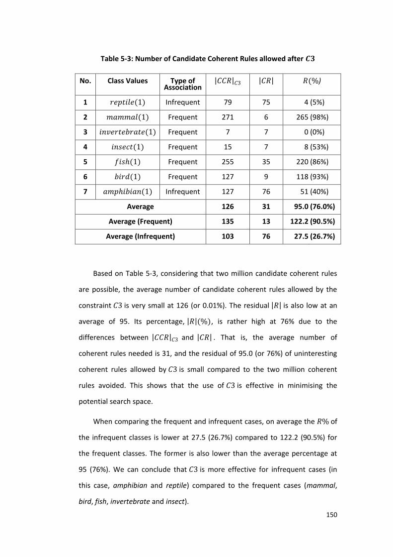
150
Table 5-3: Number of Candidate Coherent Rules allowed after 𝑪𝟑
No. Class Values Type of Association
𝐶𝐶𝑅 𝐶3 𝐶𝑅 𝑅(%)
1 𝑟𝑒𝑝𝑡𝑖𝑙𝑒(1) Infrequent 79 75 4 (5%)
2 𝑚𝑎𝑚𝑚𝑎𝑙(1) Frequent 271 6 265 (98%)
3 𝑖𝑛𝑣𝑒𝑟𝑡𝑒𝑏𝑟𝑎𝑡𝑒(1) Frequent 7 7 0 (0%)
4 𝑖𝑛𝑠𝑒𝑐𝑡(1) Frequent 15 7 8 (53%)
5 𝑓𝑖𝑠(1) Frequent 255 35 220 (86%)
6 𝑏𝑖𝑟𝑑(1) Frequent 127 9 118 (93%)
7 𝑎𝑚𝑝𝑖𝑏𝑖𝑎𝑛(1) Infrequent 127 76 51 (40%)
Average 126 31 95.0 (76.0%)
Average (Frequent) 135 13 122.2 (90.5%)
Average (Infrequent) 103 76 27.5 (26.7%)
Based on Table 5-3, considering that two million candidate coherent rules
are possible, the average number of candidate coherent rules allowed by the
constraint 𝐶3 is very small at 126 (or 0.01%). The residual 𝑅 is also low at an
average of 95. Its percentage, 𝑅 (%), is rather high at 76% due to the
differences between 𝐶𝐶𝑅 𝐶3 and 𝐶𝑅 . That is, the average number of
coherent rules needed is 31, and the residual of 95.0 (or 76%) of uninteresting
coherent rules allowed by 𝐶3 is small compared to the two million coherent
rules avoided. This shows that the use of 𝐶3 is effective in minimising the
potential search space.
When comparing the frequent and infrequent cases, on average the 𝑅% of
the infrequent classes is lower at 27.5 (26.7%) compared to 122.2 (90.5%) for
the frequent classes. The former is also lower than the average percentage at
95 (76%). We can conclude that 𝐶3 is more effective for infrequent cases (in
this case, amphibian and reptile) compared to the frequent cases (mammal,
bird, fish, invertebrate and insect).

151
5.3.2.2 Effect of 𝐶1
The additional pruning carried by the first constraint 𝐶1 is measured in
relation to 𝐶3. We disable the second constraint in the algorithm, and set
𝐿 = 16 to relax the fourth constraint 𝐶4 in order to find the combined effect in
using 𝐶1 and 𝐶3. The added effect of 𝐶1, given by 𝐶𝐶𝑅 𝐶1,𝐶3 can be found by
using equation 5.3. The experimental results are shown in Table 5-4.
Table 5-4: Number of Candidate Coherent Rules allowed after 𝑪𝟑 at 𝑾 = 𝟏
No. Class Values 𝐶𝐶𝑅 𝐶1,𝐶3 𝐶𝐶𝑅 𝐶3 𝐶𝐶𝑅 𝐶1\𝐶3
1 𝑟𝑒𝑝𝑡𝑖𝑙𝑒(1) 79 79 0
2 𝑚𝑎𝑚𝑚𝑎𝑙(1) 271 271 0
3 𝑖𝑛𝑣𝑒𝑟𝑡𝑒𝑏𝑟𝑎𝑡𝑒(1) 7 7 0
4 𝑖𝑛𝑠𝑒𝑐𝑡(1) 15 15 0
5 𝑓𝑖𝑠(1) 255 255 0
6 𝑏𝑖𝑟𝑑(1) 127 127 0
7 𝑎𝑚𝑝𝑖𝑏𝑖𝑎𝑛(1) 127 127 0
Based on Table 5-4, 𝐶𝐶𝑅 𝐶1\𝐶3 has a value of zero. In other words, 𝐶1 is not
better than 𝐶3 in finding coherent rules in any class value at 𝑊 = 1 .
Nonetheless, 𝐶1 may still be useful at smaller values of 𝑊.
To explore this supposition, the above experiment is repeated by
increasing the parameter value of 𝑊 from zero. The experimental results are
plotted in Figure 5.1 for increasing values of 𝑊.

152
Figure 5.1: Number of Additional 𝑪𝑪𝑹 avoided in using 𝑪𝟏 over 𝑪𝟑 over
Increasing 𝑾
Figure 5.1 shows the use of 𝐶1 is effective only at smaller values of 𝑊. For
example, when 𝑊 is less than or equal to 0.4 on class mammal, is less than or
equal to 0.2 on class fish, equal to 0 on class bird, or less than or equal to 0.2 on
class amphibian, then 𝐶1 is effective. The positive effect of 𝐶1 is observed in
the three most-observed animal classes, and the one most rarely-observed
animal class, in the Zoo dataset. The percentage of additional pruning is
relatively small at 5% for the infrequent animal class. In contrast, the rate of
additional pruning is high at 92% for the mammal class at 𝑊 = 0. This suggests
that constraint 𝐶1 is effective for frequent cases at small values of 𝑊.
By reducing the size of the potential search space, the use of constraint 𝐶1
in 𝐸𝑆𝑆_𝐶𝑅, together with the necessary constraint 𝐶3, accelerates the rule
generation process. The experiments demonstrate that the combination of
constraint 𝐶1 and constraint 𝐶3 reduces the number of uninteresting rules that
elude the constraints for the mammal class (compared to using 𝐶3 alone by 248
(92%)). While the use of 𝐶1 accelerates the generation of coherent rules, in
248 (92%)
192 (71%)
64 (24%)77 (30%)
39 (15%)60(47%)
6 (5%)0
50
100
150
200
250
300
w=0
w=0
.2
w=0
.4
w=0
.6
w=0
.8
w=1
Ad
dit
ion
al N
um
ber
of
CC
R A
void
ed
Improvement in using C1
Reptile
Mammal
Invertebrate
Insect
Fish
Bird
Amphibian

153
contrast, the use of the strength value constraint using a confidence measure in
𝐴𝑝𝑟𝑖𝑜𝑟𝑖 does not improve the efficiency of discovering item sets.
5.3.2.3 Effect of 𝐶2
The additional pruning carried by the second constraint 𝐶2 is measured in
relation to 𝐶3. We remove the first constraint in the algorithm, and set 𝐿 = 16
to relax the fourth constraint 𝐶4 to find 𝐶𝐶𝑅 𝐶2,𝐶3. The above experiment is
repeated by increasing the parameter value of 𝑊. The experimental results are
plotted in Figure 5.2.
Figure 5.2: Number of Additional 𝑪𝑪𝑹 avoided in using 𝑪𝟐 over 𝑪𝟑 over
Increasing 𝑾
𝐶2 is effective at smaller values of 𝑊. For example, when 𝑊 is less than or
equal to 0.4 for class mammal, is less than or equal to 0.2 for both classes fish
and amphibian, or when 𝑊 is equal to zero for class bird, then it is effective.
Similar to the constraint 𝐶1, the positive effect of 𝐶2 is observed in the three
most-observed animals, and one least-observed animal (such as the class
amphibian) in the Zoo dataset. The rate of additional pruning is high at 97% in
263 (97%)
216 (80%)
72 (27%)
108 (42%)
28 (22%)
64(50%)
0
50
100
150
200
250
300
w=0
w=0
.2
w=0
.4
w=0
.6
w=0
.8
w=1
Ad
dit
ion
al N
um
ber
of
CC
R A
void
ed
Improvement in using C2
Reptile
Mammal
Invertebrate
Insect
Fish
Bird
Amphibian

154
class mammal at 𝑊 = 0, and lower at 22% in class amphibian at 𝑊 = 0.2. This
suggests that 𝐶2 is a constraint that is effective for both frequent and
infrequent cases at small values of 𝑊, but tends to greater effectiveness for
frequent cases.
Use of constraint 𝐶2 produced a lower residual than constraint 𝐶1. The
residual using 𝐶3 for class amphibian was 127. With the use of 𝐶1, the residual
was reduced by 7 units to 120. The use of 𝐶2 would have reduced it by 28 to 99.
It appears that the use of both 𝐶1 and 𝐶2, will always substantially reduce a
residual. On class mammal, the residual is 271 using 𝐶3, and is reduced by 248
using 𝐶1 and reduced by 263 using 𝐶2. The effect of deploying 𝐶2 can be
appreciated because it reduces more candidate coherent rules than using 𝐶3
alone or a combination of 𝐶3 and 𝐶1.
Theoretically, both constraints 𝐶1 and 𝐶2 are based on 𝐻′ and 𝐻′′, which
are approximate values of the measure of interestingness 𝐻 of coherent rules.
While the measure of interestingness 𝐻 does not possess the anti-monotone
property, pruning opportunities can be exploited by using the approximates 𝐻′
and 𝐻′′. As a result, 𝐸𝑆𝑆_𝐶𝑅 can identify coherent rules with the required
strength value without needing to generate all coherent rules. The constraint
𝐶1 requires less processing time because it finds the occurrences of a single
item set using coverage (see section 4.5.2.4). The constraint 𝐶2 is more
expensive in terms of processes time because it finds the co-occurrences of two
item sets together using support values (see section 4.5.2.2). From the
experiments, we conclude that the extra processing time needed to find the
supports and compare these to the highest strength value in 𝐶2, is offset by the
reduction of residuals in both frequent and infrequent cases.

155
5.3.2.4 Effect of 𝐶4
In this section, we analyse the effect of using the fourth constraint 𝐶4, and
identify the conditions under which it is most effective. We remove the first and
second constraint by setting 𝑊 = 1. The experiment is repeated with increasing
parameter values of 𝐿. This isolates the effect of the fourth constraint 𝐶4 in
relation to 𝐶3. The experimental results are plotted in Figure 5.3.
Figure 5.3: Number of Additional 𝑪𝑪𝑹 avoided in using 𝑪𝟒 over 𝑪𝟑
The use of 𝐶4 is effective only at smaller values of 𝐿. For example, when 𝐿 is
less than or equal to 4 on both class mammal and class fish, is less than or
equal to 2 on both class bird and class amphibian, or less than or equal to 2 on
class insect and class reptile, then it is effective.
The positive effect of 𝐶4 is observed on the four most-observed animals
and the two least-observed animals (that is, amphibian and reptile) in the Zoo
dataset. It affects more classes of animals then 𝐶1 and 𝐶2. The use of 𝐶4
without a user-specified parameter (that is, at 𝐿 = 0) results in substantial
pruning. For example, the rate of additional pruning is high at 97% in class
Rep. 6 (8%)
262 (97%)
168(62%)
Ins. 7 (47%)
236 (93%)
37 (15%)
120(94%)
72 (57%)
0
50
100
150
200
250
300
L=0
L=2
L=4
L=6
L=8
L=1
0
L=1
2
L=1
4
L=1
6
Ad
dit
ion
al N
um
ber
of
CC
R A
void
ed
Improvement in using C4
Reptile
Mammal
Invertebrate
Insect
Fish
Bird
Amphibian
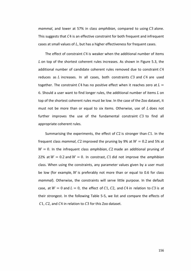
156
mammal, and lower at 57% in class amphibian, compared to using 𝐶3 alone.
This suggests that 𝐶4 is an effective constraint for both frequent and infrequent
cases at small values of 𝐿, but has a higher effectiveness for frequent cases.
The effect of constraint 𝐶4 is weaker when the additional number of items
𝐿 on top of the shortest coherent rules increases. As shown in Figure 5.3, the
additional number of candidate coherent rules removed due to constraint 𝐶4
reduces as 𝐿 increases. In all cases, both constraints 𝐶3 and 𝐶4 are used
together. The constraint 𝐶4 has no positive effect when it reaches zero at 𝐿 =
6. Should a user want to find longer rules, the additional number of items 𝐿 on
top of the shortest coherent rules must be low. In the case of the Zoo dataset, it
must not be more than or equal to six items. Otherwise, use of 𝐿 does not
further improves the use of the fundamental constraint 𝐶3 to find all
appropriate coherent rules.
Summarising the experiments, the effect of 𝐶2 is stronger than 𝐶1. In the
frequent class mammal, 𝐶2 improved the pruning by 9% at 𝑊 = 0.2 and 5% at
𝑊 = 0. In the infrequent class amphibian, 𝐶2 made an additional pruning of
22% at 𝑊 = 0.2 and 𝑊 = 0. In constrast, 𝐶1 did not improve the amphibian
class. When using the constraints, any parameter values given by a user must
be low (for example, 𝑊 is preferably not more than or equal to 0.6 for class
mammal). Otherwise, the constraints will serve little purpose. In the default
case, at 𝑊 = 0 and 𝐿 = 0, the effect of 𝐶1, 𝐶2, and 𝐶4 in relation to 𝐶3 is at
their strongest. In the following Table 5-5, we list and compare the effects of
𝐶1, 𝐶2, and 𝐶4 in relation to 𝐶3 for this Zoo dataset.

157
Table 5-5: Percentage of Additional Candidate Coherent Rules allowed in
Addition to 𝑪𝟑 at 𝑾 = 𝟎, 𝑳 = 𝟎
No. Class Values Additional pruning%
C1 C2 C4
1 𝑟𝑒𝑝𝑡𝑖𝑙𝑒(1)
(Infrequent)
0% 0% 8%*
2 𝑚𝑎𝑚𝑚𝑎𝑙(1) 92% 97%* 96.7%
3 𝑖𝑛𝑣𝑒𝑟𝑡𝑒𝑏𝑟𝑎𝑡𝑒(1) 0% 0% 0%
4 𝑖𝑛𝑠𝑒𝑐𝑡(1) 13% 13% 47%*
5 𝑓𝑖𝑠(1) 30% 42% 93%*
6 𝑏𝑖𝑟𝑑(1) 47% 50% 94%*
7 𝑎𝑚𝑝𝑖𝑏𝑖𝑎𝑛(1)
(Infrequent)
5% 22% 57%*
Average
(Infrequent)
3% 14% 38%*
Average
(Frequent)
57% 65% 93%*
* - highest among 𝐶1, 𝐶2, and 𝐶4.
In Table 5-5, the average of infrequent class filtered by 𝐶1 is calculated as the
summation of the further reduction in residuals using the constraint 𝐶1 divided
by the summation of residuals using 𝐶3. The other averages are calculated
similarly.
Table 5-5 shows that 𝐶4 often attains the highest performance of 𝐶1, 𝐶2
and 𝐶4. Also, it is suitable for use in both frequent and infrequent classes with
average additional pruning percentages of 93% and 38% respectively. We
highlight that, on average, 𝐶2 further improves 11% over 𝐶1 in infrequent
cases, and 8% in frequent classes. 𝐶1, in turn, improves 57% over 𝐶3 in
frequent classes and only 3% in infrequent classes. This shows that the use of

158
constraints in addition to 𝐶3 further minimises the search space required to
identify coherent rules that can be decoupled into association rules.
To re-emphasize, the rules discovery approach using 𝐸𝑆𝑆_𝐶𝑅 requires
neither a preset minimum support threshold nor identification of all item sets,
unlike the classic mining association rules approach. Instead, 𝐸𝑆𝑆_𝐶𝑅 uses four
constraints to selectively identify coherent rules. Constraints are imposed
sequentially within an iteration to generate coherent rules. The sequence is 𝐶3-
𝐶1-𝐶2-𝐶4. The constraint 𝐶3, which identifies coherent rules, is fundamental.
Deployment of constraints 𝐶1, 𝐶2, and 𝐶4 acts to further reduce the potential
search space. By using the anti-monotone property of each constraint, 𝐸𝑆𝑆_𝐶𝑅
selectively covers the entire space without missing any interesting association
rules or coherent rules.

159
5.4 Quality of Coherent Rules
In this section we compare the coherent rules found using 𝐸𝑆𝑆_𝐶𝑅 with
association rules found using 𝐴𝑝𝑟𝑖𝑜𝑟𝑖. Experiments are carried out using the
Zoo dataset. We use the program 𝐴𝑝𝑟𝑖𝑜𝑟𝑖 written by Borgelt [Bo08] to find
association rules. 𝐴𝑝𝑟𝑖𝑜𝑟𝑖 requires the user to pre-select a minimum support
and a minimum confidence threshold. In the following experiments, we need to
assume two reasonable and hypothetical thresholds:
(i) The minimum support threshold is set at 5% [YeLe02],[DaBhKa03],
[ChLiCh03].
(ii) The minimum confidence threshold is set at 50% [AgImSw93],
[BrMoSi97].
As a result of these assumptions, all association rules not supported by at least
5% of transaction records are considered infrequent; otherwise they are
considered frequent. We group association rules into three categories:
(i) Infrequent association rules that contain less observed classes (for
example, reptile and amphibian).
(ii) Frequent association rules that have frequently observed classes
(for example, mammal).
(iii) Negative association rules that contain at least one absence of an
attribute value.
5.4.1 Infrequent Rules
Classes reptile and amphibian, according to Table 5-2, are infrequent
because both have support values below our hypothetical 5% of minimum
support threshold. Specifically, the observation of these class attributes,
denoted using class values 𝑟𝑒𝑝𝑡𝑖𝑙𝑒(1) and 𝑎𝑚𝑝𝑖𝑏𝑖𝑎𝑛(1), are infrequent. As a

160
result, any association rule found concerning these class values will also be
infrequent. Otherwise, they are frequent association rules (that is, involving at
least 5% of support values). We execute the algorithm 𝐸𝑆𝑆_𝐶𝑅 on the latter
two class values and report the shortest coherent rules in Table 5-6. For
comparative purposes we execute the algorithm Apriori [Bo08] with the
minimum support set at 5% and minimum confidence set at 50% for the reptile
and amphibian classes.
Table 5-6: Shortest Infrequent Rules found on 𝒓𝒆𝒑𝒕𝒊𝒍𝒆 and 𝒂𝒎𝒑𝒉𝒊𝒃𝒊𝒂𝒏
No. Coherent Rules Found without
Pre-selected Threshold Settings (𝑬𝑺𝑺_𝑪𝑹)
Association Rules Found with
minsup = 5%, and
minconf = 50% (Apriori [Bo08])
1 𝑒𝑔𝑔𝑠 1 , 𝑡𝑜𝑜𝑡𝑒𝑑 1 ,𝑏𝑟𝑒𝑎𝑡𝑒𝑠(1), 𝑡𝑎𝑖𝑙(1)
⇒ 𝑟𝑒𝑝𝑡𝑖𝑙𝑒(1)
and,
¬ 𝑒𝑔𝑔𝑠 1 , 𝑡𝑜𝑜𝑡𝑒𝑑 1 ,𝑏𝑟𝑒𝑎𝑡𝑒𝑠(1), 𝑡𝑎𝑖𝑙(1)
⇒ ¬𝑟𝑒𝑝𝑡𝑖𝑙𝑒(1),
𝐻 = 0.4
None Found
2 𝑎𝑞𝑢𝑎𝑡𝑖𝑐 1 , 𝑙𝑒𝑔 4
⇒ 𝑎𝑚𝑝𝑖𝑏𝑖𝑎𝑛(1)
and,
¬ 𝑎𝑞𝑢𝑎𝑡𝑖𝑐 1 , 𝑙𝑒𝑔 4
⇒ ¬𝑎𝑚𝑝𝑖𝑏𝑖𝑎𝑛 1 , 𝐻 = 0.25
None Found
A complete list of attribute values can be found in Appendix D. These are
formatted as 𝑒𝑔𝑔𝑠(1) , 𝑡𝑜𝑜𝑡𝑒𝑑(1) , 𝑏𝑟𝑒𝑎𝑡𝑒𝑠(1) and 𝑡𝑎𝑖𝑙(1) , which mean
observation of the attributes eggs, toothed, breathes and tail respectively. On
the other hand, the attribute values 𝑟𝑒𝑝𝑡𝑖𝑙𝑒(0) and 𝑎𝑚𝑝𝑖𝑏𝑖𝑎𝑛(0) means the
attributes reptile and amphibian are not observed. The symbol ‘¬’ means the
absence of an item set in a set of transaction records. The absence of an

161
attribute (for example, reptile) with a binary value, ¬𝑟𝑒𝑝𝑡𝑖𝑙𝑒(1) is the same as
𝑟𝑒𝑝𝑡𝑖𝑙𝑒 0 . On the other hand, the absence of a set of attribute values is
mapped to a number of possible combinations. For example,
¬ 𝑒𝑔𝑔𝑠 1 , 𝑡𝑜𝑜𝑡𝑒𝑑 1 is mapped to either of 𝑒𝑔𝑔𝑠 0 , 𝑡𝑜𝑜𝑡𝑒𝑑 1 ,
𝑒𝑔𝑔𝑠 1 , 𝑡𝑜𝑜𝑡𝑒𝑑 0 , and 𝑒𝑔𝑔𝑠 0 , 𝑡𝑜𝑜𝑡𝑒𝑑 0 . The mapping is explained
in section 3.2.1.1. For simplicity, we denote a set that contains only a single
attribute value by using its attribute value because association rules are always
between two item sets. For example, we write 𝑟𝑒𝑝𝑡𝑖𝑙𝑒(1) instead of
𝑟𝑒𝑝𝑡𝑖𝑙𝑒(1) .
Referring to Table 5-6, 𝐸𝑆𝑆_𝐶𝑅 found two sets of coherent rules. If each is
decoupled into two association rules, then a total of four association rules are
found. We calculate also the support and confidence of these rules for analysis
purposes:
𝑒𝑔𝑔𝑠 1 , 𝑡𝑜𝑜𝑡𝑒𝑑 1 , 𝑏𝑟𝑒𝑎𝑡𝑒𝑠(1), 𝑡𝑎𝑖𝑙(1) ⇒ 𝑟𝑒𝑝𝑡𝑖𝑙𝑒(1)
support = 3.0% and confidence 75.0% 5.5
¬ 𝑒𝑔𝑔𝑠 1 , 𝑡𝑜𝑜𝑡𝑒𝑑 1 , 𝑏𝑟𝑒𝑎𝑡𝑒𝑠(1), 𝑡𝑎𝑖𝑙(1) ⇒ 𝑟𝑒𝑝𝑡𝑖𝑙𝑒(0)
support = 94.1% and confidence 97.9% 5.6
{𝑎𝑞𝑢𝑎𝑡𝑖𝑐 1 , 𝑙𝑒𝑔 4 } ⇒ 𝑎𝑚𝑝𝑖𝑏𝑖𝑎𝑛(1)
support = 4.0% and confidence 57.1% 5.7
¬ 𝑎𝑞𝑢𝑎𝑡𝑖𝑐 1 , 𝑙𝑒𝑔 4 ⇒ 𝑎𝑚𝑝𝑖𝑏𝑖𝑎𝑛(0)
support = 93.1% and confidence 100.0% 5.8
Association rules in equation 5.5 and 5.7 are positive association rules while
equations 5.6 and 5.8 are negative association rules. 𝐴𝑝𝑟𝑖𝑜𝑟𝑖 is incapable of
finding these association rules because they involve absence of items. Clearly,

162
association rules in equation 5.5 and 5.7 will also not be found using 𝐴𝑝𝑟𝑖𝑜𝑟𝑖
due to support values lower than our hypothetical minimum support threshold
set at 5%. The ability to find association rules below a minimum support
threshold is unique to 𝐸𝑆𝑆_𝐶𝑅. In contrast, the classic rule mining algorithm
𝐴𝑝𝑟𝑖𝑜𝑟𝑖 requires a support and confidence framework.
Within the Zoo dataset, we observe that the shortest association rule that
describe a reptile has four items in its antecedent item set. This is contrary to
our thinking that the antecedent of a rule contains only a single attribute value.
If we lower the minimum support threshold to 3%, using 𝐴𝑝𝑟𝑖𝑜𝑟𝑖, we will find
too many association rules. The shortest pseudo-implication in equation 5.5 will
be concealed among many other association rules which lack implication with
their antecedents contain a larger number of attribute values. As a result, we
lose an opportunity to identify the shortest association rules that are
implicational according to propositional logic. The practicality and advantage in
using 𝐸𝑆𝑆_𝐶𝑅 to find association rules becomes immediately apparent.
Should a user want to discover longer rules, 𝐸𝑆𝑆_𝐶𝑅 can discover a total of
55 coherent rules for both attribute values of 𝑟𝑒𝑝𝑡𝑖𝑙𝑒(1) and 𝑎𝑚𝑝𝑖𝑏𝑖𝑎𝑛(1).
Longer rules are more difficult to interpret than short rules, but the longer rules
discovered through 𝐸𝑆𝑆_𝐶𝑅 can be mapped to logical implications of
propositional logic with a support value below 5%. In contrast, Apriori cannot
discover any of these infrequent association rules. Through this experiment, we
show that a discovery process based on the classical framework may ignore
association rules needed for infrequently observed attributes.

163
5.4.2 Frequent and Interesting Rules
We repeat the experiment settings in section 5.4.1 on the most observed
class, mammal. We list their results in Table 5-7. We also list the rules found by
the 𝐴𝑝𝑟𝑖𝑜𝑟𝑖 algorithm. Rules not found by either algorithm are highlighted (in
amber). For simplicity, we write a set that contains only a single attribute value
using its attribute value without the symbol ‘ ’ because association rules are
always between two item sets. For example, we write 𝑚𝑎𝑚𝑚𝑎𝑙(1) instead of
𝑚𝑎𝑚𝑚𝑎𝑙(1) .
Table 5-7: Shortest Frequent Rules found for Class 𝒎𝒂𝒎𝒎𝒂𝒍
No. Coherent Rules Found without Pre-selected Threshold Settings
(Sort by strength value 𝐇)
Association Rules Found with
minsup = 5%,
and minconf = 50%
(Sort by confidence value )
1 𝑚𝑖𝑙𝑘(1) ⇒ 𝑚𝑎𝑚𝑚𝑎𝑙(1),
and,
𝑚𝑖𝑙𝑘(0) ⇒ 𝑚𝑎𝑚𝑚𝑎𝑙(0), 𝐻 = 1.0
𝑚𝑖𝑙𝑘(1) ⇒ 𝑚𝑎𝑚𝑚𝑎𝑙(1)
[Sup.=40.6%, Conf.=100%]
2 𝑎𝑖𝑟(1) ⇒ 𝑚𝑎𝑚𝑚𝑎𝑙(1),
and,
𝑎𝑖𝑟(0) ⇒ 𝑚𝑎𝑚𝑚𝑎𝑙(0), 𝐻 = 0.85366
𝑎𝑖𝑟(1) ⇒ 𝑚𝑎𝑚𝑚𝑎𝑙(1)
[Sup.=38.6%, Conf.=90.7%]
3 𝑙𝑒𝑔𝑠(4) ⇒ 𝑚𝑎𝑚𝑚𝑎𝑙(1),
and,
¬𝑙𝑒𝑔𝑠(4) ⇒ 𝑚𝑎𝑚𝑚𝑎𝑙(0), 𝐻 = 0.58537
𝑙𝑒𝑔𝑠(4) ⇒ 𝑚𝑎𝑚𝑚𝑎𝑙(1)
[Sup.=30.7%, Conf.=81.6%]
4 𝑐𝑎𝑡𝑠𝑖𝑧𝑒(1) ⇒ 𝑚𝑎𝑚𝑚𝑎𝑙(1),
and,
𝑐𝑎𝑡𝑠𝑖𝑧𝑒(0) ⇒ 𝑚𝑎𝑚𝑚𝑎𝑙(0), 𝐻 = 0.48780
𝑐𝑎𝑡𝑠𝑖𝑧𝑒(1) ⇒ 𝑚𝑎𝑚𝑚𝑎𝑙(1)
[Sup.=31.7%, Conf.=72.7%]
5 𝑡𝑜𝑜𝑡𝑒𝑑(1) ⇒ 𝑚𝑎𝑚𝑚𝑎𝑙(1),
and,
𝑡𝑜𝑜𝑡𝑒𝑑(0) ⇒ 𝑚𝑎𝑚𝑚𝑎𝑙(0), 𝐻 = 0.46341
𝑡𝑜𝑜𝑡𝑒𝑑(1) ⇒ 𝑚𝑎𝑚𝑚𝑎𝑙(1)
[Sup.=39.6%, Conf.=65.6%]
6 𝑑𝑜𝑚𝑒𝑠𝑡𝑖𝑐(1) ⇒ 𝑚𝑎𝑚𝑚𝑎𝑙(1)
[Sup.=7.9%, Conf.=61.5%]
7 𝑏𝑟𝑒𝑎𝑡𝑒𝑠(1) ⇒ 𝑚𝑎𝑚𝑚𝑎𝑙(1)
[Sup.=40.6%, Conf.=51.2%]

164
Based on the Table 5-7, the algorithm 𝐸𝑆𝑆_𝐶𝑅 finds five coherent rules for
mammal (or ten association rules, because each coherent rule consist of a pair
of association rules) but 𝐴𝑝𝑟𝑖𝑜𝑟𝑖 finds seven association rules. Of these seven
association rules, association rules 6 and 7 in Table 5-7 are not reported by
𝐸𝑆𝑆_𝐶𝑅. We detail the contingency tables (Table 5-8 and Table 5-9 respectively)
for these two association rules, and explain why these rules are not interesting.
Table 5-8: A Contingency Table for Attributes: domestic and mammal
Frequency of co-occurrences
𝒴
𝑚𝑎𝑚𝑚𝑎𝑙(1) 𝑚𝑎𝑚𝑚𝑎𝑙(0) Total
𝒳 𝑑𝑜𝑚𝑒𝑠𝑡𝑖𝑐(1) 8 5 13
𝑑𝑜𝑚𝑒𝑠𝑡𝑖𝑐(0) 33 55 88
Total 41 60 101
Table 5-9: A Contingency Table for Attributes: breathes and mammal
Frequency of co-occurrences
𝒴
𝑚𝑎𝑚𝑚𝑎𝑙(1) 𝑚𝑎𝑚𝑚𝑎𝑙(0) Total
𝒳 𝑏𝑟𝑒𝑎𝑡𝑒𝑠(1) 41 39 80
𝑏𝑟𝑒𝑎𝑡𝑒𝑠(0) 0 21 21
Total 41 60 101
Based on the entries in Table 5-8, the association rule:
(i) 𝑑𝑜𝑚𝑒𝑠𝑡𝑖𝑐(1) ⇒ 𝑚𝑎𝑚𝑚𝑎𝑙(1) , has a support = 7.9% and
confidence = 61.5% 5.9
is not interesting because it is largely contradicted by the other association
rules causing it to be trivial. The other association rules with stronger statistics
are:

165
(ii) 𝑑𝑜𝑚𝑒𝑠𝑡𝑖𝑐(0) ⇒ 𝑚𝑎𝑚𝑚𝑎𝑙(1) , support = 80.5% and
confidence = 37.5% 5.10
and
(iii) 𝑑𝑜𝑚𝑒𝑠𝑡𝑖𝑐(0) ⇒ 𝑚𝑎𝑚𝑚𝑎𝑙(0) , support = 54.5% and
confidence = 62.5% 5.11
These above two association rules have support values higher than 7.9%.
Reporting association rules with weaker support (in equation 5.9) while
stronger association rules exist is misleading. In addition, the rules in equations
5.10 and 5.11 are contradictory if they are reasoned as logical implications. That
is, if ‘not domestic’ (𝑑𝑜𝑚𝑒𝑠𝑡𝑖𝑐(0)) is associated with mammals, then it cannot
be associated with ‘not mammal’. Hence, these rules are not reported by
𝐸𝑆𝑆_𝐶𝑅 as implicational association rules.
𝐴𝑝𝑟𝑖𝑜𝑟𝑖, however, reports that mammal is a domestic animal (Table 5-7,
row 6), and identifies this relationship as one of the strongest association rules
with a confidence of 61.5%. In fact, there are 41 sets of mammal (such as
buffalo, bear, elephant; refer to Appendix C) but only 8 of them are domestic
animals. Many more mammals (that is, 33 or 80.5%) are not domestic. The
latter is never highlighted; instead a weaker rule is reported. If this weaker rule
is used in a business application it could cause a wrong decision. 𝐸𝑆𝑆_𝐶𝑅 avoids
reporting this misleading association rule.
In another case, based on Table 5-9, the association rule:
𝑏𝑟𝑒𝑎𝑡𝑒𝑠(1) ⇒ 𝑚𝑎𝑚𝑚𝑎𝑙(1) , support = 40.6% and confidence = 51.2% 5.12

166
is not interesting enough because this association rule exists on its own and
cannot be supported by any other association rules. Theoretically, association
rules in equation 5.12 are meaningfully supported by:
𝑏𝑟𝑒𝑎𝑡𝑒𝑠(0) ⇒ 𝑚𝑎𝑚𝑚𝑎𝑙(0) 5.13
That is, if “breathes using lungs” is a fundamental characteristic of mammals,
then logically speaking, an animal that does not breathe using lungs is not a
mammal; however, the association rule in 5.13 (with support 20.8%) does not
occur frequently enough. A detailed study shows the association rule in 5.13 is
contradicted by the following association rule with a stronger existence:
𝑏𝑟𝑒𝑎𝑡𝑒𝑠(1) ⇒ 𝑚𝑎𝑚𝑚𝑎𝑙(0) , support = 38.6% and confidence = 48.8% 5.14
Hence the association rule in 5.13 is suppressed from complementing the
meaning on a positive association rule in equation 5.12. 𝐸𝑆𝑆_𝐶𝑅 does not
report single positive association rules that cannot be supported by a negative
association rule because this indicates the positive association rule,
𝑏𝑟𝑒𝑎𝑡𝑒𝑠(1) ⇒ 𝑚𝑎𝑚𝑚𝑎𝑙(1), is not strong enough to be a pseudo-implication
of equivalence.
In addition, based on Table 5-9, while 41 sets of animals that breath using
lungs are associated to mammal, this characteristic is also associated to 39 sets
of non-mammals (that is, all animals except fish). The use of this characteristic
(𝑏𝑟𝑒𝑎𝑡𝑒𝑠(1)) is too statistically weak to describe a mammal.
The association rule in equation 5.14 is also not reported by 𝐸𝑆𝑆_𝐶𝑅
because it contradicts the association rule in equation 5.12. Logically, if
mammals breathe using lungs, then they cannot be described as breathing
without lungs. Furthermore, the association rule in equation 5.14 is not
supported by any other association rule.

167
In addition to the five shortest coherent rules found in Table 5-7, the
algorithm 𝐸𝑆𝑆_𝐶𝑅 can discover coherent rules of all sizes. By setting 𝐿 = 16 to
discover coherent rules of all sizes, the algorithm 𝐸𝑆𝑆_𝐶𝑅 finds 25,442
coherent rules for mammal. In comparison, the algorithm 𝐴𝑝𝑟𝑖𝑜𝑟𝑖 finds a
maximum of only 715 association rules (of all sizes).
5.4.3 Negative Rules
𝐸𝑆𝑆_𝐶𝑅 can discover negative rules in both its first and second phase.
Negative association rules can be found by:
(i) Decoupling the coherent rule pairs found from the first phase of
the algorithm 𝐸𝑆𝑆_𝐶𝑅, where each positive rule is paired with a
negative rule.
(ii) Decoupling the coherent rule pairs found from the second phase,
where each decoupled rule is a negative rule.
In contrast, Apriori cannot discover any negative rules. 𝐴𝑝𝑟𝑖𝑜𝑟𝑖 finds only the
association among items that are present in transaction records, or attributes
that can be observed in the classification dataset.
We decouple all the negative association rules from coherent rule pairs in
Table 5-7, and execute 𝐸𝑆𝑆_𝐶𝑅 in its second phase. The results are shown in
Table 5-10.

168
Table 5-10: The Shortest Negative Coherent Rules found, where 𝒀 =
{′𝒎𝒂𝒎𝒎𝒂𝒍′}
No. Decoupled Negative Rules from Coherent Rules discovered via the
First Phase of 𝑬𝑺𝑺_𝑪𝑹
Decoupled Negative Rules from Coherent Rules discovered via the
Second Phase of 𝑬𝑺𝑺_𝑪𝑹
1 𝑚𝑖𝑙𝑘(0) ⇒ 𝑚𝑎𝑚𝑚𝑎𝑙(0),
𝐻 = 1.0
𝑒𝑔𝑔𝑠(1) ⇒ 𝑚𝑎𝑚𝑚𝑎𝑙(0),
𝐻 = 0.92683
2 𝑎𝑖𝑟(0) ⇒ 𝑚𝑎𝑚𝑚𝑎𝑙(0),
𝐻 = 0.85366
𝑒𝑔𝑔𝑠(0) ⇒ 𝑚𝑎𝑚𝑚𝑎𝑙(1),
𝐻 = 0.92683
3 ¬𝑙𝑒𝑔𝑠(4) ⇒ 𝑚𝑎𝑚𝑚𝑎𝑙(0),
𝐻 = 0.58537
4 𝑐𝑎𝑡𝑠𝑖𝑧𝑒(0) ⇒ 𝑚𝑎𝑚𝑚𝑎𝑙(0),
𝐻 = 0.48780
5 𝑡𝑜𝑜𝑡𝑒𝑑(0) ⇒ 𝑚𝑎𝑚𝑚𝑎𝑙(0),
𝐻 = 0.46341
As shown in Table 5-10, 𝐸𝑆𝑆_𝐶𝑅 discovered all seven shortest negative
association rules that cannot be discovered by Apriori. These rules have high
coherent strength values denoting that this phenomenon happens logically and
strongly. Among these:
(i) Animals that do not lay eggs are usually mammals (𝐻 = 0.93).
(ii) Animals that do not produce milk are not mammals (𝐻 = 1).
This knowledge cannot be discovered by using 𝐴𝑝𝑟𝑖𝑜𝑟𝑖 on the Zoo dataset.
We repeated the above procedure to find the shortest negative rules for
the infrequent classes reptile and amphibian. The results are reported in Table
5-11.

169
Table 5-11: The Shortest Negative Coherent Rules found, where 𝒀 =
{′𝒓𝒆𝒑𝒕𝒊𝒍𝒆′} and 𝒀 = {′𝒂𝒎𝒑𝒉𝒊𝒃𝒊𝒂𝒏′}
No. Decoupled Negative Rules from Coherent Rules discovered via the
First Phase of 𝑬𝑺𝑺_𝑪𝑹
Decoupled Negative Rules from Coherent Rules
discovered via the
Second Phase of 𝑬𝑺𝑺_𝑪𝑹
1 ¬ 𝑒𝑔𝑔𝑠 1 , 𝑡𝑜𝑜𝑡𝑒𝑑 1 , 𝑏𝑟𝑒𝑎𝑡𝑒𝑠 1 , 𝑡𝑎𝑖𝑙 1
⇒ 𝑟𝑒𝑝𝑡𝑖𝑙𝑒(0), 𝐻 = 1.0
𝑁𝑜𝑛𝑒 𝐹𝑜𝑢𝑛𝑑
2 ¬ 𝑎𝑞𝑢𝑎𝑡𝑖𝑐 1 , 𝑙𝑒𝑔 4
⇒ 𝑎𝑚𝑝𝑖𝑏𝑖𝑎𝑛(0), 𝐻 = 0.85366
𝑁𝑜𝑛𝑒 𝐹𝑜𝑢𝑛𝑑
We conclude that 𝐸𝑆𝑆_𝐶𝑅 can discover negative association rules from both
frequent and infrequent classes.
It is possible to augment 𝐴𝑝𝑟𝑖𝑜𝑟𝑖 so that it recognises the absence of items.
One of the approaches is to supply the absence of an attribute value in the
dataset [CoYaZhCh06]. 𝐴𝑝𝑟𝑖𝑜𝑟𝑖 will recognise this negative value as an attribute
value; however, this approach will cause an increased number of association
rules to be found. An increase in the number of association rules found results
in contradictory association rules (such as those highlighted in Table 5-8 and in
equations 5.10 and 5.11). This large volume deteriorates the quality of the
overall rules set as more rules are not interesting. In another approach, a new
measure of interestingness, lift [GeHa06] can be used to augment 𝐴𝑝𝑟𝑖𝑜𝑟𝑖.
Each generated association rules is measured for its 𝑙𝑖𝑓𝑡 value. If the value of
lift falls below the value of 1, then these rules are negatively correlated [Au04].
Instead of 𝑋 ⇒ 𝑌 , negative association rules 𝑋 ⇒ ¬𝑌 are reported. This
augmented approach, however, does not find all negative association rules such
as ¬𝑋 ⇒ 𝑌 and ¬𝑋 ⇒ ¬𝑌 . Because 𝐴𝑝𝑟𝑖𝑜𝑟𝑖 finds only positive association
rules, as a result, this augmented approach will only find part of the negative

170
association rules. A third approach, based on the Chi-squared Test, was
proposed by Brin, Motwani and Silverstein [BrMoSi97] as a new mining
framework. Although this framework discovers both positive and negatively-
correlated rules, it is still limited by the availability of an approach to search for
correlated rules without a minimum support threshold. In addition, the Chi-
squared Test is constrained by a statistical requirement that at least 80% of the
cells in a contingency table have a value greater than five. In practice, this
requirement is rarely met [BrMoSi97]. In addition, all infrequently-correlated
rules will be lost below this minimum support threshold.
The concept of coherent rules does not require a minimum support
threshold to be defined. It also discovers pairs of association rules, where at
least one of the rules is a negative association rule 14. Consequently, the
coherent rules concept offsets the disadvantages of finding association rules
above a minimum support threshold and among items or attribute values that
can be observed.
5.4.4 Distinct Features of 𝐸𝑆𝑆_𝐶𝑅
This section summarises the features of 𝐸𝑆𝑆_𝐶𝑅 compared to 𝐴𝑝𝑟𝑖𝑜𝑟𝑖.
Unlike 𝐴𝑝𝑟𝑖𝑜𝑟𝑖, 𝐸𝑆𝑆_𝐶𝑅:
(i) Does not require a preset minimum support threshold. 𝐸𝑆𝑆_𝐶𝑅
does not require a preset a minimum support threshold to find
association rules. Coherent rules are found based on mapping to
14 If a given dataset contains only the presence of items, then the negative association rules according to Wu, Zhang and Zhang [WuZhZh04] are discovered (See section 2.2.1). Otherwise, if a dataset contains both the presence and absence of items, where each of the absence of items is viewed as a new item, then a second type of negative association rules according to Cornelis et al. [CoYaZhCh06] are discovered.

171
logical equivalences. From the coherent rules, we can decouple
the pair for two pseudo-implications of equivalences. The latter
can be used as association rules with the property that each rule
can be further mapped to a logical equivalence.
(ii) Does not need to generate frequent item sets. 𝐸𝑆𝑆_𝐶𝑅 does not
need to generate frequent item sets. Nor does it need to generate
the association rules within each item set. Instead, 𝐸𝑆𝑆_𝐶𝑅 finds
coherent rules directly. Coherent rules are found within the small
number of candidate coherent rules allowed through its
constraints.
(iii) Identifies complete set of coherent rules. 𝐸𝑆𝑆_𝐶𝑅 identifies a
complete set of coherent rules. By default, it identifies the shortest
and strongest coherent rules, but it can identify coherent rules of
all sizes and strength values. On the other hand, 𝐴𝑝𝑟𝑖𝑜𝑟𝑖 identifies
association rules that have at least a minimum support threshold.
In the case that a minimum support threshold is heuristically set,
complete solutions may not obtained. In addition, the shortest and
strongest association rules can only be discovered alongside
association rules of different sizes and strengths. And
consequently the shortest and strongest association rules may be
difficult to detect, will require further filtering to be discovered,
and waste resources in having to discover all sizes.
(iv) Identifies negative association rules. 𝐸𝑆𝑆_𝐶𝑅, by default, also
identifies negative association rules. Given a set of transaction
records that does not indicate item absence, 𝐴𝑝𝑟𝑖𝑜𝑟𝑖 cannot
identify negative association rules. 𝐸𝑆𝑆_𝐶𝑅 finds the negative
pseudo-implications of equivalences and uses them to
complement both the positive and negative rules found.

172
5.5 𝑬𝑺𝑺_𝑪𝑹 Performance
5.5.1 Effect of Parameter Values on the Number of
Coherent Rules Discovered
In this section, we establish an experiment to investigate the ability of the
algorithm 𝐸𝑆𝑆_𝐶𝑅 to discover coherent rules under different parameter values.
We vary the parameters 𝐿 and 𝑊 used in algorithm 𝐸𝑆𝑆_𝐶𝑅 to find an arbitrary
number of coherent rules. The parameter 𝐿 ranges from 0 to 16, where the
latter is the total number of attributes of animals in the Zoo dataset. By setting
𝐿 = 0, algorithm 𝐸𝑆𝑆_𝐶𝑅 finds only the shortest coherent rules; however, by
setting 𝐿 = 16, algorithm 𝐸𝑆𝑆_𝐶𝑅 will find all coherent rules regardless of their
size because all sizes of coherent rules are allowed. The parameter 𝑊 is varied
from 0 to 1, where at 𝑊 = 0 algorithm 𝐸𝑆𝑆_𝐶𝑅 finds coherent rules with the
strongest strength values, and at 𝑊 = 1 algorithm 𝐸𝑆𝑆_𝐶𝑅 finds coherent rules
with any positive strength values.
The experimental results for each class are shown in two figures, Figure 5.4
and Figure 5.5:

173
Figure 5.4: Number of Coherent Rules discovered using different Parameter
Values for 𝑳 at 𝑾 = 𝟎
Figure 5.5: Number of Coherent Rules discovered using different Parameter
Values for 𝑾 at 𝑳 = 𝟎
0
5
10
15
20
25
30
35
40
45
L=0 L=2 L=4 L=6 L=8 L=10 L=12 L=14 L=16
Nu
mb
er o
f C
oh
eren
t R
ule
s
|CR| vs. L
Reptile
Mammal
Invertebrate
Insect
Fish
Bird
Amphibian
0
1
2
3
4
5
6
w=0 w=0.2 w=0.4 w=0.6 w=0.8 w=1.0
Nu
mb
er o
f C
oh
eren
t R
ule
s
|CR| vs. W
Reptile
Mammal
Invertebrate
Insect
Fish
Bird
Amphibian

174
Experimental results show that the algorithm 𝐸𝑆𝑆_𝐶𝑅 at its default parameter
values (𝐿 = 0 and 𝑊 = 0) finds the most effectual (that is, the shortest and the
strongest) coherent rules. Should a user want to discover weaker and longer
coherent rules, increasing the value of 𝐿 and 𝑊 will also increase the number of
coherent rules discovered. The increase in the number of coherent rules stops
at certain combinations of parameter values, thus indicating that all possible
coherent rules with arbitrary size and strength values have been discovered.
In the next two sections, we investigate the cost (in terms of time) of
finding coherent rules as the parameter values 𝐿 and 𝑊 increase.

175
5.5.2 Effect of Parameter 𝐿 Value vs. Time
In section 5.5.1 we saw that enhancing parameter value 𝐿 increased the
number of coherent rules discovered. In this section, we investigate the
discovery time associated with the increase of coherent rules discovered.
We supply a series of parameter values for 𝐿 in an increasing order from
𝐿 = 0 to 𝐿 = 16 to the algorithm 𝐸𝑆𝑆_𝐶𝑅. For each experiment on a class, a
different parameter 𝑊 is supplied from 0 to 1 at an interval of 0.2. Hence, we
have the discovery time at an increasing parameter value of 𝐿 with seven
different parameter values of 𝑊. These are shown in Figure 5.6, Figure 5.7,
Figure 5.8, Figure 5.9, Figure 5.10, Figure 5.11 and Figure 5.12 for each animal
class. The number of coherent rules found is shown on the secondary axis for
reference.
Figure 5.6: Coherent Rules found, where 𝒀 = {′𝒓𝒆𝒑𝒕𝒊𝒍𝒆′}
From Figure 5.6, the performance of 𝐸𝑆𝑆_𝐶𝑅 at an increasing parameter value
of 𝐿 is not obvious because only four coherent rules are discovered.
0
1
2
3
4
5
0
0.05
0.1
0.15
0.2
0.25
0.3
0.35
0.4
0.45
0.5
Nu
mb
er
of
CR
(at
W=1
)
Tim
e (S
ec.)
Increase of L Vs. Time (Class: Reptile)
W=0
W=0.2
W=0.4
W=0.6
W=0.8
W=1.0
|CR| at W=1
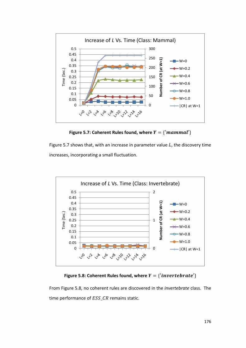
176
Figure 5.7: Coherent Rules found, where 𝒀 = {′𝒎𝒂𝒎𝒎𝒂𝒍′}
Figure 5.7 shows that, with an increase in parameter value 𝐿, the discovery time
increases, incorporating a small fluctuation.
Figure 5.8: Coherent Rules found, where 𝒀 = {′𝒊𝒏𝒗𝒆𝒓𝒕𝒆𝒃𝒓𝒂𝒕𝒆′}
From Figure 5.8, no coherent rules are discovered in the invertebrate class. The
time performance of 𝐸𝑆𝑆_𝐶𝑅 remains static.
0
50
100
150
200
250
300
0
0.05
0.1
0.15
0.2
0.25
0.3
0.35
0.4
0.45
0.5
Nu
mb
er
of
CR
(at
W=1
)
Tim
e (S
ec.)
Increase of L Vs. Time (Class: Mammal)
W=0
W=0.2
W=0.4
W=0.6
W=0.8
W=1.0
|CR| at W=1
0
1
2
0
0.05
0.1
0.15
0.2
0.25
0.3
0.35
0.4
0.45
0.5
Nu
mb
er
of
CR
(at
W=1
)
Tim
e (S
ec.)
Increase of L Vs. Time (Class: Invertebrate)
W=0
W=0.2
W=0.4
W=0.6
W=0.8
W=1.0
|CR| at W=1

177
Figure 5.9: Coherent Rules found, where 𝒀 = {′𝒊𝒏𝒔𝒆𝒄𝒕′}
From Figure 5.9, the performance of 𝐸𝑆𝑆_𝐶𝑅 at an increasing parameter value
of 𝐿 is not obvious because only eight coherent rules are discovered.
Figure 5.10: Coherent Rules found, where 𝒀 = {′𝒇𝒊𝒔𝒉′}
In Figure 5.10, the experimental results show that, with an increase in
parameter value 𝐿 , the discovery time increases, incorporating a small
fluctuation.
0
1
2
3
4
5
6
7
8
9
0
0.05
0.1
0.15
0.2
0.25
0.3
0.35
0.4
0.45
0.5
Nu
mb
er
of
CR
(at
W=1
)
Tim
e (S
ec.)
Increase of L Vs. Time (Class: Insect)
W=0
W=0.2
W=0.4
W=0.6
W=0.8
W=1.0
|CR| at W=1
0
50
100
150
200
250
0
0.05
0.1
0.15
0.2
0.25
0.3
0.35
0.4
0.45
0.5
Nu
mb
er
of
CR
(at
W=1
)
Tim
e (S
ec.)
Increase of L Vs. Time (Class: Fish)
W=0
W=0.2
W=0.4
W=0.6
W=0.8
W=1.0
|CR| at W=1

178
Figure 5.11: Coherent Rules found, where 𝒀 = {′𝒃𝒊𝒓𝒅′}
From Figure 5.11, the experimental results show that, at an increasing
parameter value 𝐿, the discovery time also increases, incorporating a small
fluctuation.
Figure 5.12: Coherent Rules found, where 𝒀 = {′𝒂𝒎𝒑𝒉𝒊𝒃𝒊𝒂𝒏′}
0
20
40
60
80
100
120
140
0
0.05
0.1
0.15
0.2
0.25
0.3
0.35
0.4
0.45
0.5
Nu
mb
er
of
CR
(at
W=1
)
Tim
e (S
ec.)
Increase of L Vs. Time (Class: Bird)
W=0
W=0.2
W=0.4
W=0.6
W=0.8
W=1.0
|CR| at W=1
0
10
20
30
40
50
60
0
0.05
0.1
0.15
0.2
0.25
0.3
0.35
0.4
0.45
0.5
Nu
mb
er
of
CR
(at
W=1
)
Tim
e (S
ec.)
Increase of L Vs. Time (Class: Amphibian)
W=0
W=0.2
W=0.4
W=0.6
W=0.8
W=1.0
|CR| at W=1

179
Overall the experimental results show that, with an increase of parameter
value 𝐿 , the discovery time increases. The increase incorporates a small
fluctuation. The general trend of increased time is linked to the availability of
coherent rules in the dataset. When many coherent rules are available (for
example, in class mammal), the discovery time increases sharply but plateaus
after all coherent rules are discovered after 𝐿 = 6; hence, it is not as expensive
as a linear increase of discovery time. On the other hand, when few coherent
rules are available (for example, in classes reptile, invertebrate and insect), the
increase is almost unnoticeable.
The trace of fluctuations in discovery time is due to two reasons:
(i) An increasing parameter 𝐿, allows greater checking of candidate
coherent rules 𝑋. .𝑌. Some of the candidate coherent rules 𝑋. .𝑌
do not meet the anti-monotone constraint and can be avoided. As
a result, 𝐸𝑆𝑆_𝐶𝑅 also avoids the large number of candidate
coherent rules containing the superset 𝑋𝐸. .𝑌 . This exclusion
decreases discovery time; however, the reduction does not always
happen because an increase of 𝐿 also invites an exponential large
number of candidate coherent rules and thus expands discovery
time. This increase and decrease is one cause of the fluctuations in
discovery time.
(ii) 𝐸𝑆𝑆_𝐶𝑅 is constructed using the program Matlab, which employs
matrix optimisation to facilitate internal calculation. The
experiment at 𝐿 = 2 is executed after 𝐿 = 0 , where matrix
optimisation may have taken effect. Thus, a small (that is, within
0.05 seconds) reduction within the overall discovery time is
observed.

180
Experimental results also show that the rate of increase in the discovery
time for each 𝐿 value is influenced by the parameter value 𝑊 used. With
reference to class mammal at 𝐿 = 16, the increase in discovery time (at 𝑊 = 0)
is almost unnoticeable, but at 𝑊 = 1 (maximum value of 𝑊), the increase in
discovery time it is about seven times greater. This is due to the increased
number of coherent rules available at this large value of 𝑊.
5.5.3 Effect of Parameter 𝑊 vs. Time
In this section, we measure the effect of an increase in parameter value 𝑊
over time. A higher 𝑊 value discovers more coherent rules with reduced
strength values. The experiment is performed on each class value. Parameter
values for 𝐿 range from 0 to 16, and are set at an interval of 2. The discovery
time is plotted in Figure 5.13, Figure 5.14, Figure 5.15, Figure 5.16, Figure 5.17,
Figure 5.18 and Figure 5.19 for each of the class values. The number of coherent
rules found using 𝐿 = 16 is shown on the secondary axis.

181
Figure 5.13: Effect of 𝑾 vs. Time, where 𝒀 = {′𝒓𝒆𝒑𝒕𝒊𝒍𝒆′}
The number of coherent rules associated with class reptile is low at 4; the time
performance is not obvious at an increasing parameter value of 𝑊.
Figure 5.14: Effect of 𝑾 vs. Time, where 𝒀 = {′𝒎𝒂𝒎𝒎𝒂𝒍′}
The number of coherent rules associated with class mammal is among the
highest; the discovery time increases at an increasing parameter value of 𝑊.
0
1
2
3
4
5
0
0.05
0.1
0.15
0.2
0.25
0.3
0.35
0.4
0.45
0.5
W=0 W=0.2 W=0.4 W=0.6 W=0.8 W=1.0
Tim
e (S
ec.)
Increase of W Vs. Time (Class: Reptile)
L=0
L=2
L=4
L=6
L=8
L=10
L=12
L=14
L=16
0
50
100
150
200
250
300
0
0.05
0.1
0.15
0.2
0.25
0.3
0.35
0.4
0.45
0.5
W=0 W=0.2 W=0.4 W=0.6 W=0.8 W=1.0
Tim
e (S
ec.)
Increase of W Vs. Time (Class: Mammal)
L=0
L=2
L=4
L=6
L=8
L=10
L=12
L=14

182
Figure 5.15: Effect of 𝑾 vs. Time, where 𝒀 = {′𝒊𝒏𝒗𝒆𝒓𝒕𝒆𝒃𝒓𝒂𝒕𝒆′}
There is no coherent rule associated with class invertebrate. Consequently, the
time performance is not obvious at an increasing parameter value of 𝑊.
Figure 5.16: Effect of 𝑾 vs. Time, where 𝒀 = {′𝒊𝒏𝒔𝒆𝒄𝒕′}
The number of coherent rules associated with class insect is low at 8. Thus, the
time performance is not obvious at an increasing parameter value of 𝑊.
0
1
2
0
0.05
0.1
0.15
0.2
0.25
0.3
0.35
0.4
0.45
0.5
W=0 W=0.2 W=0.4 W=0.6 W=0.8 W=1.0
Tim
e (S
ec.)
Increase of W Vs. Time (Class: Invertebrate)
L=0
L=2
L=4
L=6
L=8
L=10
L=12
L=14
L=16
0
1
2
3
4
5
6
7
8
9
0
0.05
0.1
0.15
0.2
0.25
0.3
0.35
0.4
0.45
0.5
W=0 W=0.2 W=0.4 W=0.6 W=0.8 W=1.0
Tim
e (S
ec.)
Increase of W Vs. Time (Class: Insect)
L=0
L=2
L=4
L=6
L=8
L=10
L=12
L=14
L=16
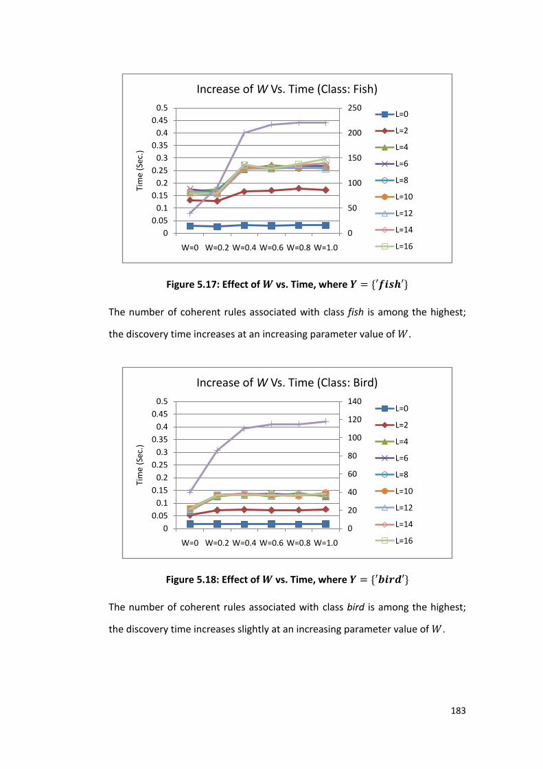
183
Figure 5.17: Effect of 𝑾 vs. Time, where 𝒀 = {′𝒇𝒊𝒔𝒉′}
The number of coherent rules associated with class fish is among the highest;
the discovery time increases at an increasing parameter value of 𝑊.
Figure 5.18: Effect of 𝑾 vs. Time, where 𝒀 = {′𝒃𝒊𝒓𝒅′}
The number of coherent rules associated with class bird is among the highest;
the discovery time increases slightly at an increasing parameter value of 𝑊.
0
50
100
150
200
250
0
0.05
0.1
0.15
0.2
0.25
0.3
0.35
0.4
0.45
0.5
W=0 W=0.2 W=0.4 W=0.6 W=0.8 W=1.0
Tim
e (S
ec.)
Increase of W Vs. Time (Class: Fish)
L=0
L=2
L=4
L=6
L=8
L=10
L=12
L=14
L=16
0
20
40
60
80
100
120
140
0
0.05
0.1
0.15
0.2
0.25
0.3
0.35
0.4
0.45
0.5
W=0 W=0.2 W=0.4 W=0.6 W=0.8 W=1.0
Tim
e (S
ec.)
Increase of W Vs. Time (Class: Bird)
L=0
L=2
L=4
L=6
L=8
L=10
L=12
L=14
L=16

184
Figure 5.19: Effect of 𝑾 vs. Time, where 𝒀 = {′𝒂𝒎𝒑𝒉𝒊𝒃𝒊𝒂𝒏′}
With an increase of parameter value 𝑊, in general, the discovery time also
increases. In some cases, fluctuations can be observed within 0.05 second. For
example, in class reptile, the discovery time reduces slightly at 𝐿 = 0, while 𝑊
increases from 0.4 to 0.8. A similar reduction in discovery time with an increase
parameter 𝑊 can be observed in class fish at 𝐿 = 16 while 𝑊 increases from
0.4 to 0.6. Use of the larger window (brought about by larger values of 𝑊)
allows more checking of candidate coherent rules for the anti-monotone
property. Consequently, it becomes faster to find the (final) minimum strength
value, 𝑚𝑖𝑛_. Once the final minimum strength value is found, the constraints
avoid unnecessary candidate coherent rules. With a smaller window (that is,
decreased values of 𝑊 ), the constraints avoid some, but not all, of the
candidate coherent rules that are not part of the final solution. The 𝐸𝑆𝑆_𝐶𝑅
algorithm requires slightly more time to reach the final 𝑚𝑖𝑛_; however, this
observation may not always hold true. In most cases, with an increase in
parameter value 𝑊, the time required to check a large number of candidate
coherent rules for actual coherent rules is usually offset by the positive effect of
0
10
20
30
40
50
60
0
0.05
0.1
0.15
0.2
0.25
0.3
0.35
0.4
0.45
0.5
W=0 W=0.2 W=0.4 W=0.6 W=0.8 W=1.0
Tim
e (S
ec.)
Increase of W Vs. Time (Class: Amphibian)
L=0
L=2
L=4
L=6
L=8
L=10
L=12
L=14
L=16
|CR| at L=16

185
finding the final value of 𝑚𝑖𝑛_ faster. An increase in parameter value 𝑊
typically increases discovery time.
The general increase of discovery time is also subject to the availability of
coherent rules in a dataset. In the experiment on class reptile, class invertebrate
and class insect where the number of available coherent rules is less than ten,
the increase in discovery time is small. It is larger on classes such as mammal,
bird and fish. Nonetheless, in class fish, even with a constant number of
available coherent rules, the discovery time increases at 𝑊 = 1.0 and 𝐿 = 1.0.
Parameter 𝑊 controls the constraints 𝐶1 and 𝐶2 . At 𝑊 = 1 , these anti-
monotone constraints are relaxed, thus resulting an increase in discovery time.

186
5.5.4 Increase of Time over Number of Attribute Values
In this section, we measure the effect of an increase in the number of
attribute values over time. The Zoo dataset has twenty-one attribute values in
total. We find coherent rules for each class using a controlled number of
attribute values. The discovery time is plotted in Figure 5.20.
Figure 5.20: Increase in Time over Number of Attribute Values ( 𝑰 )
Experimental results show that an increase in the number of attribute
values exponentially increases discovery time. Increased discovery time is most
often observed on the frequent classes (mammal, fish and bird), followed by
the infrequent classes (amphibian and reptile), at |𝐼| = 21. This perhaps implies
that 𝐸𝑆𝑆_𝐶𝑅 performs faster when finding coherent rules in infrequent classes;
however, at 𝐼 < 21, the discovery time on frequent and infrequent class is
almost identical.
The discovery time for class amphibian increases gradually to less than 0.1
second at |𝐼| = 11 and remains the same at |𝐼| = 13; after that it increases to
0.15 second and plateaus. Similarly, the discovery time for other classes also
0
0.05
0.1
0.15
0.2
0.25
0.3
0.35
0.4
0.45
0.5
Tim
e (
Sec.
)
Increase of N vs. Time (L=16, W=1)
Reptile
Mammal
Invertebrate
Insect
Fish
Bird
Amphibian

187
follows the pattern of increase-stop-increase. The discovery time for class
mammal increases gradually and stabilises between 𝐼 = 15 to 𝐼 = 17 before
increasing to less than 0.4 second at 𝐼 = 21. The discovery time for class fish,
for example, plateaus between 𝐼 = 13 to 𝐼 = 17 and increases sharply at
𝐼 = 19 before stabilising at 0.3 second. The increase of discovery time is
mainly due to the availability of coherent rules. The greater the number of
coherent rules that can be mined from the dataset, the more discovery time is
needed. If no additional coherent rules are available for discovery, the discovery
time almost plateaus. We further analyse this by plotting, in Figure 5.21, the
number of coherent rules against an increase in the number of attribute values.
Figure 5.21: Increase in Coherent Rules over Number of Attribute Values ( 𝑰 )
The graphs in Figure 5.20 and Figure 5.21 show similar patterns. The
increase in the number of attribute values results in an increase of coherent
rules. To discover more coherent rules, more time is required; otherwise the
discovery time mostly plateaus with some exceptions in class reptile, class insect
and class invertebrate. The latter three classes have very few coherent rules
available for discovery; however, some discovery time is spent on them even
0 0 4 40
50
100
150
200
250
300
350
400
450
500
Nu
mb
er
of
Co
he
ren
t R
ule
s
|CR| vs. N (L=16, W=1)
Reptile
Mammal
Invertebrate
Insect
Fish
Bird
Amphibian

188
though no coherent rules are discovered. In class reptile, for example, the
discovery time increases slightly from 𝐼 = 7 to 𝐼 = 13 but reports no
coherent rules. This is not surprising given the exponential increase of search
space brought by an increase of 𝐼 . The increase of time is less than 0.1 second
and does not show any exponential trait when no coherent rules are available
from the dataset. Once coherent rules are found at 𝐼 = 19, the discovery time
increases and then plateaus. We can summarise that the 𝐸𝑆𝑆_𝐶𝑅 discovery
time grows with the number of coherent rules available from the dataset. If no
coherent rules are available, then the discovery time is at its minimum. This
shows a desirable characteristic of 𝐸𝑆𝑆_𝐶𝑅 when performing operations on the
Zoo dataset.
As a result of the findings discussed in section 5.5.3 section 5.5.4, we
summarise that the discovery time typically increases almost linearly with
parameter values 𝐿 and 𝑊 , and the number of attribute values, but
fundamentally is limited by the coherent rules available. An increase in the
parameter values 𝐿 and 𝑊 typically increases linearly the number of coherent
rules available. The rate of increase is maintained before slowing gradually to a
stop as shown in Figure 5.4 and Figure 5.5. The discovery process in terms of
time displays the same trait; however, an increase in the number of attribute
values exponentially increases the number of coherent rules (shown in Figure
5.21). The discovery time for coherent rules almost linearly follows the same
trait.
In this section we have explored the relationships between the parameters
𝐿 and 𝑊, discovery time and attribute values. In the next section, we test
𝐸𝑆𝑆_𝐶𝑅 to determine whether it can find coherent rules in real-world
transaction records involving large numbers.

189
5.6 Discovering Coherent Rules on Real-world
Market Basket Transaction Records
In this section, we test 𝐸𝑆𝑆_𝐶𝑅 to discover coherent rules in real-world
transaction records. These transaction records are obtained from the Frequent
Item Set Repository [Go06]. BMS-View1, BMS-View2 and BMS-Pos are three
transaction records from three retail stores used in the KDD CUP 2000
competition, [KoBrFrMaZh00][KoBrFrMaZh00]. Retail is a retail market basket
dataset supplied by an anonymous Belgian retail supermarket store
[BrSwVaWe99]. We summarise the statistics from these four sets of transaction
records in the following table.
Table 5-12: Summary of the Statistics on Transaction Records (TC) used
TC Total Unique Items in
TC
Total Records
Average Number of Items Per TC
Maximum Number of Items Per TC
Description
BMS-View1
497 59,602 2.5 267 Several months of “click-stream” data from an e-commerce web site. Each transaction in this dataset is a web session where a certain product is viewed.
BMS-View2
3,340 77,512 4.6 161 See BMS-View1; another “click-stream” dataset.
BMS- POS
1,657 515,600 6.5 164 A collection of several years of point-of-sale data.
Retail 16,470 88,162 10.3 76 Retail market basket data from an anonymous Belgian retail store.
We use the algorithm 𝐸𝑆𝑆_𝐶𝑅 to find coherent rules on each of these sets of
data. For each set of transaction records, we obtained a list containing unique

190
items. A random seven items are used as consequence item sets. Different
parameter values of 𝐿 and 𝑊 were used to discover coherent rules. The
experimental results show the average number of coherent rules found on the
seven items (|𝐶𝑅|), and 𝐸𝑆𝑆_𝐶𝑅’s average discovery time in seconds (𝑆𝑒𝑐.).
Table 5-13: Real World Retail Transaction Records
Transaction Records
Parameter value 𝑾
𝐋 = 𝟎* 𝐋 = 𝟏
|CR| Sec. |CR| Sec.
BMS-View1 ( I = 497) 𝑊 = 0* 2 7 14 7
𝑊 = 0.5 2 6 14 7
𝑊 = 1.0 2 6 14 7
BMS-POS ( I = 1,657) 𝑊 = 0* 4 613 147 636
𝑊 = 0.5 4 610 147 632
𝑊 = 1.0 4 611 147 632
BMS-View2 ( I = 3,340) 𝑊 = 0* 0 79 0 79
𝑊 = 0.5 0 80 0 80
𝑊 = 1.0 0 79 0 80
Retail ( I = 16,470) 𝑊 = 0* 16 931 115 920
𝑊 = 0.5 16 932 115 922
𝑊 = 1.0 16 932 115 922
Average 𝑾 = 𝟎* 6 408 69 411
𝑾 = 𝟎.𝟓 6 407 69 410
𝑾 = 𝟏.𝟎 6 407 69 410
*: default parameter values

191
5.6.1 Observations
The experimental results showed that the transaction records contain
varying numbers of coherent rules, and that some transaction records contain
no coherent rules. For example, Retail contained more coherent rules than the
other sets of transaction records, while BMS-View2 lacked coherent rules. We
cannot learn rules from a dataset such as BMS-View2 if the dataset does not
have the rules with the statistics and structure of coherent rules. If the coherent
rules found were at their maximum strength value ‘𝐻 = 1’, then an increase of
parameter value 𝑊 did not increase the number of coherent rules found. On
the other hand, an increase in the parameter value 𝐿 increased the number of
longer coherent rules. In BMS-POS, this increase in the number of coherent
rules was 36.75 times, in Retail 7.1 times, and in BMS-View 7 times. As a result,
the discovery time also increased by 3.75% in BMS-POS and 1.2% in Retail but
remained almost unchanging in BMS-View1 because the number of coherent
rules available was small at 14.
Overall, when new coherent rules were available, discovery time increased
as parameter value 𝐿 increased. On the other hand, when no new coherent
rules were available, the discovery time remained almost static over an
increased parameter value. An average of six shortest and strongest coherent
rules was discovered in 408 seconds.
5.6.2 Finding of Coherent Rules
The experimental results show that the algorithm 𝐸𝑆𝑆_𝐶𝑅 is able to find
coherent rules in a very large search space. This confirms the theoretical
prediction in sections 4.5 and 4.6 that we can find coherent rules by using anti-
monotone constraints. The Belgium supermarket dataset (Retail dataset), for

192
example, has 16,470 items. To search for a complete set of coherent rules,
𝐸𝑆𝑆_𝐶𝑅 needed to consider around 5 × 104957 possible candidate coherent
rules for each consequence item set. 𝐸𝑆𝑆_𝐶𝑅 uses four anti-monotone
constraints to avoid generating all candidate coherent rules exhaustively.
𝐸𝑆𝑆_𝐶𝑅 , at its default setting, is able to identify the most effectual
coherent rules, which are the shortest coherent rules with the strongest
strength value. Complete sets of coherent rules are also found. A detailed
analysis of the coherent rules discovered in the Retail dataset using parameter
values 𝑊 = 0 and 𝐿 = 0 showed the shortest coherent rules item set 𝑋
contained two items. The strongest strength value of 𝐻 was ‘1’. At other
parameter values, 𝐸𝑆𝑆_𝐶𝑅 found other coherent rules with values and sizes of
increasing strength. It is interesting that many coherent rules with a strength
value ‘1’ were found from transaction records signifying they are most
interesting. For each antecedent item set in these coherent rules, we can
infallibly predict whether or not the consequence item set will occur. These
rules perfectly predict and describe the potential combinations of item sets that
co-occur with the consequence item set.
Changes in parameter 𝑊 do not have a significant effect on the discovery
time, because the number of coherent rules is limited and most of them are
valued at ‘1’. Hence, the discovery time required to find coherent rules of any
strength value, compared to the discovery time required to find coherent rules
with high strength value, has no significant difference. Nonetheless,
occasionally an increase in parameter 𝑊 reduces the discovery time slightly
instead of increasing it. Internally, the use of a wider window allows more
checking of candidate coherent rules (𝑋. .𝑌). Generation of candidate coherent
rules that do not contain the anti-monotone property can thus be avoided. As a
result, the checking also enables the early preclusion of large number of
candidate coherent rules containing the superset 𝑋𝐸. .𝑌 much earlier. By

193
imposing 𝑊 = 0, the checking is limited due to the narrower window. Some
anti-monotone property exclusion opportunities are lost; however, this does
not always happen because an increase of 𝑊 often involves an exponentially
large number of candidate coherent rules, thus increasing discovery time.
Changes in parameter 𝐿 typically also increase the discovery time to find
longer coherent rules. An exception was observed in the Belgium supermarket
dataset, Retail dataset, where the discovery time reduced. The reasons are
similar to the changes in parameter 𝑊. The effect of an increase in candidate
coherent rules is less significant than the opportunities created by using
constraints incorporating anti-monotone properties.
5.6.3 Finding of Infrequent and Negative Association
Rules
The experimental results show that coherent rules can be discovered
without the need to pre-set a minimum support threshold. Each coherent rule
can be decoupled into two association rules. These rules include infrequent
rules and negative association rules. A detailed analysis shows the discovery of
a coherent rule in Retail in equation 5.15:
𝐼𝑡𝑒𝑚 260 , 𝑖𝑡𝑒𝑚 1,238 ⇒ {𝑖𝑡𝑒𝑚 16,470 } and,
¬{𝐼𝑡𝑒𝑚 260 , 𝑖𝑡𝑒𝑚(1,238)} ⇒ ¬{𝑖𝑡𝑒𝑚(16,470)}
5.15

194
This coherent rule, if decoupled, has statistics as shown in Table 5-14. The
first association rule shows:
if item indexed 260 and 1238 is observed together,
then item indexed 16,470 is also observed. 5.16
The first association rule has only one transaction record (0.0011%) to support
it. Nonetheless, this is not trivial, due to the following reasons:
(i) The first association rule is supported by the second association
rule, which implies the first in a negative way. That is:
if items indexed 260 and 1238 are not observed together,
then item indexed 16,470 is also not observed.
5.17
The coherent rule implies:
(a) if item indexed 260 is not observed and item indexed 1238 is
observed, then item indexed 16,470 is not observed.
(b) if item indexed 260 is observed and item indexed 1238 is not
observed, then item indexed 16,470 is not observed.
(c) if item indexed 260 is not observed and item indexed 1238 is
not observed, then item indexed 16,470 is not observed.
Any possible combination of items on the antecedent item set
(except the combination shown in the first association rule) that is
associated with item indexed 16,470 is not observed.
In a negative sense, any combination of items on the
antecedent item set that is not associated with the absence of
item indexed 16,470, must be associated with the observation of

195
the latter item. This is a negative sense of equation 5.16. In
addition, the second association rule that complements the first
has both very high support (99.99%) and confidence (100.0%).
Almost all transaction records in Retail support the infrequent
association rule shown in equation 5.16.
(ii) Being a part of coherent rule pair, no other negative association
rules have statistics strong enough to contradict both the first and
second association rules in retail transaction records. Both the two
association rules remain the strongest associations between item
sets {𝑖𝑡𝑒𝑚 260, 𝑖𝑡𝑒𝑚 1238} and {𝑖𝑡𝑒𝑚 16470}.
(iii) The first association rule, in itself, has a confidence value of 100%.
This indicates, most likely, that this pattern will be repeated in
future transaction records.
Classical association algorithms such as 𝐴𝑝𝑟𝑖𝑜𝑟𝑖 typically do not find association
rules with very low minimum support whence the search time is long. This is
due to the exponentially large search space and diluted meaning on association
rules reported when too many uninteresting rules are also reported. Nor do
classical association algorithms discover negative association rules.
Table 5-14: A Coherent Rule found in Retail Transaction Records
No. Pseudo-implication of Equivalence
Coherent Rules
Strength Value
Sup.
(%)
Conf. (%)
1 {𝐼𝑡𝑒𝑚 260 , 𝑖𝑡𝑒𝑚(1,238)}
⇒ {𝑖𝑡𝑒𝑚 16,470 } 1
0.0011
(1 record)
100.0
2 ¬{𝐼𝑡𝑒𝑚 260 , 𝑖𝑡𝑒𝑚(1,238)}
⇒ ¬{𝑖𝑡𝑒𝑚 16,470 } 1
0.9999
(88,161 records)
100.0

196
5.7 Conclusion
We conclude, from analysing the constraints in 𝐸𝑆𝑆_𝐶𝑅, that it is effective
to use a series of four constraints sequentially within a single phase to generate
coherent rules. At default values, or at small parameter values specified by a
user, the constraints avoid large numbers of candidate coherent rules that
cannot result in solutions. The use of constraints in sequence meets the
theoretical assumption that each constraint improves the fundamental use of
the constraint, which is based on a condition of coherent rules. Experiments
with the Zoo dataset uphold the validity of these concepts.
Technically, the number of association rules that can be found is limited if
the approach to find association rules uses a minimum support threshold. We
show that 𝐸𝑆𝑆_𝐶𝑅 is free from this disadvantage of finding association rules
that cannot be discovered using a classical approach incorporating the
infrequent and negative association rules. In addition, 𝐸𝑆𝑆_𝐶𝑅 avoids
association rules that are uninteresting due to their contradictory
characteristics and lack of implication according to propositional logic.
𝐸𝑆𝑆_𝐶𝑅 is unique in its ability to identify the shortest association rules with
the strongest strength value. 𝐸𝑆𝑆_𝐶𝑅 can be used also to find longer and
weaker association rules where appropriate parameter values are supplied by a
user. The performance of 𝐸𝑆𝑆_𝐶𝑅 to discover association rules is best at small
or no parameter values. This ability of 𝐸𝑆𝑆_𝐶𝑅 to discover rules reflects the
effective use of the anti-monotone property exploited in the condition, strength
and size of coherent rules. The quality of rules discovered is further
strengthened by the positive results from experiments carried out on four real-
world and large datasets. In sum, 𝐸𝑆𝑆_𝐶𝑅 is a suitable algorithm to discover
association rules without a minimum support threshold.

197
In this chapter, we performed a series of experiments on various datasets
and tested four facets of the 𝐸𝑆𝑆_𝐶𝑅 algorithm: its ability to limit search space;
its capacity to discover quality rules; its efficiency with respect to changing
values; and it efficiency in discovering coherent rules in real-world and large
retail transactional datasets. The next chapter concludes the thesis by
summarising the research and delineating its contribution. The thesis closes by
examining the need and possibilities for future research.

198
Chapter 6
CONCLUSION
6.1 Research Summary
In the data mining field, association rules have been researched for more
than fifteen years; however the degree to which the support threshold
effectively discovers interesting association rules has received little attention.
There is no universal standard on what constitutes the ideal minimum support
threshold. The use of a minimum support threshold results in the loss of
interesting association rules if this threshold is set inaccurately. Moreover, the
association rules discovered typically do not include item sets that are
infrequently observed nor item sets that are absent in a set of transaction
records. Consequently, the loss of interesting association rules is almost
inevitable.
In this thesis, we use mapping to logical equivalences according to
propositional logic to discover all interesting association rules, without loss.
These association rules include item sets that are frequently and infrequently
observed in a set of transaction records in addition to item sets that are absent
in each transaction record. In addition to a complete set of rules being
considered, these association rules can also be reasoned as logical implications
because they inherit propositional logic properties. Having considered both

199
infrequent and absent items, as well as being implicational, these newly-
discovered association rules are distinguished from typical association rules.
These new association rules reduce the risks associated with using an
incomplete set of association rules for decision making, as follows:
(i) Our new set of association rules considers all possible combinations
of item sets that are both present and absent in each transaction
record. It is misleading to report an incomplete set of rules and at
the same time create a sense that all available rules have been found.
The latter misleads a decision maker into thinking that only these
rules are available which in turn will lead a decision maker to reason
with incomplete information. In contrast, our algorithm results in a
full set of rules, giving the user confidence that the information
resulting from data mining activities is complete.
(ii) Our new set of association rules can identify the strongest rules.
Prior algorithms could not guarantee that the strongest association
rules found were indeed the strongest as it was possible that the
strongest rule could have been among hidden rules. Because all
possible combinations of item sets are considered, users can be
confident that the strongest rules have been found, and
consequently, the information resulting from data mining activities is
correct.
(iii) Our new set of association rules avoids reporting that item 𝐴 is
associated with item 𝐵 if there is a stronger association between
item 𝐴 and the absence of item 𝐵. Using prior association rules that
do not consider this situation could lead a user to erroneous
conclusions about the relationships among items in a dataset. Again,
identifying the strongest rule will promote information correctness
and appropriate decision making.

200
The risks associated with incomplete rules are reduced fundamentally because
our association rules are created without the user having to identify a minimum
support threshold, and because absent items have been considered. Among the
large number of association rules, only those that can be mapped to logical
equivalences according to propositional logic are considered interesting and
reported. The deliverables from this research are detailed in the next section.
6.2 Research Contributions
Our research has resulted in a novel framework, a measure of
interestingness on coherent rules and an algorithm to generate the most
interesting coherent rules from a given dataset. The discovery of coherent rules
is important because through coherent rules, a complete set of interesting
association rules that are also implicational according to propositional logic can
be discovered. The search for coherent rules has considered both the presence
and absence of items in each transaction record without requiring a user to
preset a minimum support threshold. In contrast, an association rule is typically
not implicational according to propositional logic, and the many approaches
used to output association rules has lost rules involving absent and/or
infrequent item sets. A coherent rules mining framework can thus be
appreciated for its ability to discover rules that are both implicational and
complete according to propositional logic from a given dataset.
We have created a measure of interestingness in this research. This new
measure, based on the concept of proportional error reduction, quantifies the
strength value of coherent rules and derived association rules. This research
effort is important because typically logical equivalences are not quantified for
their interestingness. These implications are either true or false according to
propositional logic. The newly-derived measure enables comparison of the most

201
interesting coherent rules. In addition, the measure is an asymmetrical measure
that considers the position of item sets, the direction of an implicational rule
and the distribution of a consequence item set. This distinguishes it from the
many measures of interestingness that do not inherit these properties and do
not measure the real implication of a rule.
The algorithm to generate coherent rules restricts the exponentially large
search space by exploiting the anti-monotone property of coherent rules.
Further strategies to prune the search space based on the constraints imposed
by (i) the strength values of coherent rules and (ii) the sizes of coherent rules
were exploited. These resulted in an efficient algorithm to generate the most
interesting coherent rules, without requiring a user to supply any parameter
values to the algorithm. This algorithm was extended to consider mining of all
coherent rules with arbitrary size and strength values. The extended algorithm
enables a user to specify, through a percentage, the window and strength value
required without knowing the strongest nor shortest coherent rules. In other
words, the user does not need domain knowledge.
In summary, the desirable features of this algorithm are:
(i) It does not require a preset minimum support threshold. Instead,
coherent rules are found based on mapping to logical
equivalences.
(ii) It does not need to generate and store a large number of
frequent item sets. Coherent rules are generated without storing a
large number of candidate item sets in computer memory. Instead,
coherent rules are generated immediately by reference to a binary
numeral system that (virtually) indexes all elements of the power-
set required.

202
(iii) It identifies a complete set of coherent rules. By default, the
algorithm identifies the shortest and strongest coherent rules from
a complete set of coherent rules. Nonetheless, it can also identify
coherent rules of all sizes and strength values.
(iv) It identifies negative association rules. By default, the algorithm
discovers the negative pseudo-implications of equivalences and
uses them to complement both the positive and negative rules
found.
Experiments show that the algorithm discovers coherent rules faster than
classic data mining algorithms at low window and size values. In the worst case
where large window and size values are required, the algorithm relies on the
anti-monotone property that is based on the condition of coherent rules to
prune the search space.
In the next section we highlight future work on the coherent rules mining
framework.
6.3 Future Work
The coherent rules mining framework and the support and confidence
framework share a common goal of discovering interesting association rules.
The former has a larger search space among the positive and negative
association rules to report association rules that can be reasoned as logical
implications. Many of the extensions of a support and confidence framework
are applicable also to a coherent rules mining framework. For example, a typical
research project on association rule mining is to search for association rules
efficiently. We consider the FP-Pattern approach [HaPeYi00] to be a potential
extension appropriate for coherent rules searching without needing to perform

203
multiple scans on a database, and thereby avoiding loading the entire data into
memory. It would also be interesting to exploit pruning properties such as
monotone properties to discover coherent rules.
Another possible extension to the coherent rules mining framework is to
consider the statistical significance test in generating coherent rules. A detailed
study on the topic of statistical tests is required to identify a suitable test. The
use of the Chi-square test, for example, is not suitable because it does not work
well on large sets of transaction records, where some cells in a contingency
table have very low support [BrMoSi97]. Coherent rules that pass some
statistical significance test would be interesting and not likely to exist by
chance.
It is possible to utilise and apply a coherent rules mining framework to
discover coherent rules that deviate from user expectations. These deviations
are important to show significant differences between coherent rules that are
logically implied from a dataset and the rules according to user expectation. For
example, authors in [JaSi04] used a Bayesian Network to inject background
knowledge and compared for deviations. Finding these deviations could
summarise the knowledge we need to know about an application domain.
In propositional logic, there are several modes of implication. We have
restricted our research to consider only the logical equivalences. It is also
possible to map association rules to the implication mode of material
implication. A logical equivalence is a subset to material implication. Finding
association rules without a minimum support threshold by mapping to material
implications could find more association rules because material implications are
less constrained. The possibility of this future work based on material
implication is depicted in Figure 6.1.

204
A coherent ruleAn association
rule-pair
Scope of this research
Proposedfuture work
Material implications
A pair of two pseudo-implications of equivalences forms a coherent rule
A pair of two pseudo-implications of material implication forms an association rule-pair
Association rules
Pseudo-implications
map to propositional logic implications (based on comparison between supports)
map to a mode of implication in propositional logic(i.e. logical equivalence)
Pseudo-implications of equivalences
Figure 6.1: Future Work based on Pseudo-implications
Association rules found from decoupling pairs of pseudo-implications mapped
to material implications are also pseudo-implications that have material
implication properties. We have begun some work in this direction [SiInSr08a],
[SiInSr08b].
This study suggests that our framework for discovering coherent rules
offers a technique for data mining that overcomes the limitations associated
with existing methods and enables finding association rules among the
presence and/or absence of a set of items without a preset minimum support
threshold. The results justify continuing research in this area in order to
increase the body of scientific knowledge of data mining specifically association
rules, and to provide practical support to those involved in data mining
activities.

205
REFERENCES
[Af08] Afify, A. (2008). Association rules discovery in manufacturing: A case study in the metal industry. 4th IPROMS Virtual International Conference. Retrieved 22th September 2008 from http://conference.iproms.org/association_rules_discovery_in_manufacturing_a_case_study_in_the_metal_industry
[AgYu98] Aggarwal, C. C., & Yu, P. S. (1998). A new framework for itemset generation. Proceedings of the 17th ACM SIGACT-SIGMOD-SIGART Symposium on Principles of Database Systems (PODS '98). pp. 18-24.
[AgImSw93] Agrawal, R., Imielinski, T., & Swami, A. (1993). Mining association rules between sets of items in large databases. SIGMOD Record, 22(2), pp. 207-216.
[AgSr94] Agrawal, R., & Srikant, R. (1994). Fast algorithms for mining association rules in large databases. Proceedings of the 20th International Conference on Very Large Data Bases. pp. 487-499
[AnZa04] Antonie, M.-L., & Zaïane, O. R. (2004). Mining positive and negative association rules: an approach for confined rules. In Knowledge Discovery in Databases: PKDD2004: Springer Berlin / Heidelberg. Vol. 3202, pp. 27-38.
[Au04] Auslender, L. E. (2004). On analytical tools for market basket (associations) analysis. Market Basket Analysis. Retrieved 22th August 2008 from http://nymetro.chapter.informs.org/prac_cor_pubs/Ausleder-On-market-basket-analysis-May-04.pdf
[BaHaZa03] Babbie, E., Halley, F., & Zaino, J. (2003). Adventures in social research, data analysis using SPSS 11.0/11.5 for Windows. Thousand Oaks: Pine Forge Press.

206
[BaPa99] Bay, S. D., & Pazzani, M. J. (1999). Detecting change in categorical data: mining contrast sets. Proceedings of the 5th ACM SIGKDD International Conference on Knowledge Discovery and Data Mining (KDD). pp. 302-306.
[BaAgGu99] Bayardo Jr., R. J., Agrawal, R., & Gunopulos, D. (1999). Constraint-based rule mining in large, dense databases. Proceedings of the 15th International Conference on Data Engineering. pp. 188-197.
[Bl72] Blalock, H. M. (1972). Social statistics. New York: McGraw-Hill Book Company.
[BlGuBrGr05] Blanchard, J., Guillet, F., Briand, H., & Gras, R. (2005). Assessing rule interestingness with a probabilistic measure of deviation from equilibrium. Proceedings of the 11th International Symposium on Applied Stochastic Models and Data Analysis (ASMDA-2005). pp. 191-200.
[Bo08] Borgelt, C. (2008). Apriori - Association rule induction / frequent item set mining. Retrieved 22nd September 2008, 2008, from http://www.borgelt.net/apriori.html
[BrSwVaWe99] Brijs, T., Swinnen, G., Vanhoof, K., & Wets, G. (1999). Using Association Rules for Product Assortment Decisions: A Case Study. In Knowledge Discovery and Data Mining. pp. 254-260.
[BrMoSi97] Brin, S., Motwani, R., & Silverstein, C. (1997). Beyond market baskets: generalizing association rules to correlations. Proceedings of the 1997 ACM Sigmod International Conference on Management of Data. pp. 265-276.
[BrMoUlTs97] Brin, S., Motwani, R., Ullman, J. D., & Tsur, S. (1997). Dynamic itemset counting and implication rules for market basket data. SIGMOD Record, 26(2), pp. 255-264.

207
[Br07a] Britannica, E. (2007). Analytic proposition. Encyclopaedia Britannica. Retrieved 1st March 2008 from http://www.britannica.com/eb/article-9007348
[Br07b] Britannica, E. (2007). Condition. Encyclopaedia Britannica. Retrieved 1st March 2008 from http://www.britannica.com/eb/article-9025123
[Br07c] Britannica, E. (2007). Epistemology: Necessary and contingent propositions. Encyclopaedia Britannica. Retrieved 1st March 2008 from http://www.britannica.com/eb/article-247953
[Br08a] Britannica, E. (2008). Equivalence. Encyclopaedia Britannica. Retrieved 5th January 2008 from http://www.britannica.com/eb/article-9032852/equivalence
[Br08b] Britannica, E. (2008). Implication. Encyclopedia Britannica. Retrieved 5th January 2008 from http://www.britannica.com/eb/article-9042218/implication
[Br08c] Britannica, E. (2008). Variable: Mathematics and logics. Encyclopaedia Britannica. Retrieved 1st November 2008 from http://www.britannica.com/EBchecked/topic/623322/variable
[BrSpHaWaJoMo98] Brossette, S. E., Sprague, A. P., Hardin, J. M., Waites, K. B., Jones, W. T., & Moser, S. A. (1998). Association rules and data mining in hospital infection control and public health surveillance. Journal of American Medical Informatics Association, 5(4), pp. 373-381.
[BuBr07] Budi, I., & Bressan, S. (2007). Application of association rules mining to named entity recognition and co-reference resolution for the Indonesian language. International Journal of Business Intelligence and Data Mining, 2(4), pp. 426-446.

208
[ChZa03] Cheung, W., & Zaïane, O. R. (2003). Incremental mining of frequent patterns without candidate generation or support constraint. Proceedings of the 7th International Database Engineering and Applications Symposium (IDEAS’03). pp. 111-116.
[ChLiCh03] Chiu, S., Liao, W.-k., & Choudhary, A. (2003). Design and evaluation of distributed smart disk architecture for IO-intensive workloads. In Computational Science - ICCS 2003: Springer Berlin / Heidelberg. Vol. 2660, pp. 230-241.
[CoTaTuXu05] Cong, G., Tan, K.-L., Tung, A. K. H., & Xu, X. (2005). Mining top-K covering rule groups for gene expression data. Proceedings of the 2005 ACM SIGMOD International Conference on Management of Data. pp. 670-681.
[CoYaZhCh06] Cornelis, C., Yan, P., Zhang, X., & Chen, G. (2006). Mining positive and negative association rules from large databases. Proceedings of the IEEE Conference on Cybernetics and Intelligent Systems. pp. 1-6.
[DaTa04] Daly, O., & Taniar, D. (2004). Exception rules mining based on negative association rules. In Computational Science and Its Applications - ICCSA 2004: Springer Berlin / Heidelberg. Vol. 3046, pp. 543-552.
[DaBhKa03] Das, A., Bhattacharyya, D. K., & Kalita, J. K. (2003). Horizontal vs. vertical partitioning in association rule mining: A comparison. Proceedings of the 6th International Conference on Computational Intelligence and Natural Computation (CINC). pp. 1617-1620.
[DoPeDiZh00] Dong, J., Perrizo, W., Ding, Q., & Zhou, J. (2000). The application of association rule mining to remotely sensed data. Proceedings of the 2000 ACM symposium on Applied computing - Volume 1. pp. 340-345.
[DoSuHaHo06] Dong, X., Sun, F., Han, X., & Hou, R. (2006). Study of positive and negative association rules based on multi-

209
confidence and Chi-squared test. In Advanced Data Mining and Applications: Springer Berlin / Heidelberg. Vol. 4093, pp. 100-109.
[DuZhFa08] Du, Y., Zhao, M., & Fan, G. (2008). Research on application of improved association rules algorithm in intelligent QA system. Proceedings of the 2008 Second International Conference on Genetic and Evolutionary Computing. pp. 414-417.
[EnTu06] Encheva, S., & Tumin, S. (2006). Application of association rules in education. In Intelligent Control and Automation: Springer Berlin / Heidelberg. Vol. 344, pp. 834-838.
[Fo90] Forsyth, R. (1990). Zoo dataset. Retrieved 5th January 2007, from Orange, AI Lab: http://magix.fri.uni-lj.si/orange/doc/datasets/zoo.htm
[FrLe06] Frankfort-Nachmias, C., & Leon-Guerrero, A. (2006). Social statistics for a diverse society. Thousand Oaks, California: Pine Forge Press.
[FrPiMa92] Frawley, W. J., Piatetsky-Shapiro, G., & Matheus, C. J. (1992). Knowledge discovery In databases: An overview. AI Magazine, 13(3), pp. 57-70.
[GaZhWa06] Gan, M., Zhang, M., & Wang, S. (2006). Extended negative association rules and the corresponding mining algorithm. In Advances in Machine Learning and Cybernetics: Springer Berlin / Heidelberg. Vol. 3930, pp. 159-168.
[GeHa06] Geng, L., & Hamilton, H. J. (2006). Interestingness measures for data mining: A survey. ACM Computing Survey, 38(3), pp. article no.9 (32 pages).
[Go06] Goethals, B. (2003). Frequent itemset mining dataset repository. Retrieved 5th January 2007, from Frequent Itemset Mining Implementations (FIMI) Repository: http://fimi.cs.helsinki.fi/data/

210
[GoKr54] Goodman, L. A., & Kruskal, W. H. (1954). Measures of association for cross classifications. Journal of the American Statistical Association, 49(268), pp. 732-764.
[HaKa06] Han, J., & Kamber, M. (2006). Data mining: Concepts and techniques: Morgan Kaufmann Publishers.
[HaPeYi00] Han, J., Pei, J., & Yin, Y. (2000). Mining frequent patterns without candidate generation. Proceedings of the 2000 ACM SIGMOD International Conference on Management of Data. pp. 1-12.
[HaWaLuTz02] Han, J., Wang, J., Lu, Y., & Tzvetkov, P. (2002). Mining top.K frequent closed patterns without minimum support. Proceedings of the 2002 IEEE International Conference on Data Mining (ICDM). pp. 211-218.
[HeBaBo99] Healey, J. F., Babbie, E. R., & Boli, J. (1999). Exploring social issues : using SPSS for Windows 95, versions 7.5, 8.0, or higher. Thousand Oaks, California: Pine Forge Press.
[Hu03] Hu, Y.-H. (2003). An efficient algorithm for discovering and maintenance of frequent patterns with multiple minimum supports. Unpublished Master Thesis, National Central University.
[HuCh06] Hu, Y.-H., & Chen, Y.-L. (2006). Mining association rules with multiple minimum supports: a new mining algorithm and a support tuning mechanism. Decision Support Systems, 42(1), pp. 1-24.
[HuKrLiWu06] Huang, W., Krneta, M., Lin, L., & Wu, J. (2006). Association bundle - A new pattern for association analysis. Proceedings of the 6th IEEE International Conference on Data Mining Workshops. pp. 601-605.
[HuGuBr05] Huynh, X.-H., Guillet, F., & Briand, H. (2005). ARQAT: An exploratory analysis tool for interestingness measures. Proceedings of the 11th International Symposium on

211
Applied Stochastic Models and Data Analysis (ASMDA '05). pp. 334-344.
[HuGuBr06] Huynh, X.-H., Guillet, F., & Briand, H. (2006). Evaluating interestingness measures with linear correlation graph. In Advances in Applied Artificial Intelligence: Springer Berlin / Heidelberg. Vol. 4031, pp. 312-321.
[In05a] Intel Corporation (2005). Moore's law 40th anniversary press kit. Moore’s Law: Raising the Bar. Retrieved 1st December 2008 from http://download.intel.com/museum/Moores_Law/Printed_Materials/Moores_Law_Backgrounder.pdf
[In05b] Intel Corporation (2005). Moore's law 40th anniversary press kit. Moore's Law Timeline, 1-1. Retrieved 1st December 2008 from http://download.intel.com/pressroom/kits/events/moores_law_40th/MLTimeline.pdf
[JaSi04] Jaroszewicz, S., & Simovici, D. A. (2004). Interestingness of frequent itemsets using Bayesian networks as background knowledge. Proceedings of the 10th ACM SIGKDD International Conference on Knowledge Discovery and Data Mining (KDD). pp. 178–186.
[Jo98] Jones, W. T. (1998). Public health surveillance using association rules. ACM SIGBIO Newsletter, 18(3), pp. 6-6.
[KoRo05] Koh, Y. S., & Rountree, N. (2005). Finding sporadic rules using apriori-inverse. In Lecture Notes in Computer Science: Advances in Knowledge Discovery and Data Mining: Springer Berlin / Heidelberg. Vol. 3518, pp. 97-106.
[KoRoOk06a] Koh, Y. S., Rountree, N., & O'Keefe, R. A. (2006). Finding non-coincidental sporadic rules using apriori-inverse. International Journal of Data Warehousing and Mining, 2(2), pp. 38-54.

212
[KoRoOk06b] Koh, Y. S., Rountree, N., & O'Keefe, R. A. (2006). Mining interesting imperfectly sporadic rules. In Advances in Knowledge Discovery and Data Mining: Springer Berlin / Heidelberg. Vol. 3918, pp. 473-482.
[KoRoOk08] Koh, Y. S., Rountree, N., & O'Keefe, R. A. (2008). Mining interesting imperfectly sporadic rules. Knowledge and Information Systems, 14(2), pp. 179-196.
[KoBrFrMaZh00] Kohavi, R., Brodley, C., Frasca, B., Mason, L., & Zheng, Z. (2000). KDD-Cup 2000 Organizers' report: Peeling the onion. SIGKDD Explorations Newsletter, 2(2), pp. 86-93.
[Kv81] Kviz, F. J. (1981). Interpretating proportional reduction in error measures as percentage of variation explained. The Sociological Quarterly, 22(3), pp. 413-420.
[LeVaMeLa07] Lenca, P., Vaillant, B., Meyer, P., & Lallich, S. (2007). Association rule interestingness measures: Experimental and theoretical studies. In Quality Measures in Data Mining: Springer Berlin / Heidelberg. Vol. 43, pp. 51-76.
[Li06] Li, J. (2006). On optimal rule discovery. IEEE Transactions on Knowledge and Data Engineering, 18(4), pp. 460-471.
[LiZh03] Li, J., & Zhang, Y. (2003). Direct interesting rule generation. Proceedings of the 3rd IEEE International Conference on Data Mining. pp. 155-162.
[Li83] Liebetrau, A. M. (1983). Measures of association. Newbury Park, CA: Sage Publications.
[LiTsSu02] Lin, W.-Y., Tseng, M.-C., & Su, J.-H. (2002). A confidence-lift support specification for interesting associations mining. Proceedings of the 6th Pacific-Asia Conference on Advances in Knowledge Discovery and Data Mining (PAKDD). pp. 148-158.

213
[LiHsChMa00] Liu, B., Hsu, W., Chen, S., & Ma, Y. (2000). Analyzing the subjective interestingness of association rules. IEEE Intelligent Systems, 15(5), pp. 47-55.
[LiHsMa99] Liu, B., Hsu, W., & Ma, Y. (1999). Mining association rules with multiple minimum supports. Proceedings of the 5th ACM SIGKDD International Conference on Knowledge Discovery and Data Mining (KDD). pp. 337-341.
[LiMaWoYu03] Liu, B., Ma, Y., Wong, C. K., & Yu, P. S. (2003). Scoring the data using association rules. Applied Intelligence, 18(2), pp. 119-135.
[Ma98] Mannila, H. (1998). Database methods for data mining, Proceedings of the 4th International Conference on Knowledge Discovery and Data Mining (Tutorial). New York, NY: IEEE.
[McCh07] McIntosh, T., & Chawla, S. (2007). High confidence rule mining for microarray analysis. IEEE/ACM Transactions on Computational Biology and Bioinformatics (TCBB), 4(4), pp. 611-623.
[Me03] Meyer, P. (2003). Two aspects of user centered data analysis and decision Aid: Quality measures for association rules and multiple criteria sorting. Unpublished DEA Thesis, University of Luxembourg.
[MuKuSa03] Murai, T., Kudo, Y., & Sato, Y. (2003). Association rules and Dempster-Shafer theory of evidence. In Discovery Science: Springer Berlin / Heidelberg. Vol. 2843, pp. 377-384.
[MuNaSa01] Murai, T., Nakata, M., & Sato, Y. (2001). A note on conditional logic and association rules. Proceedings of the Joint JSAI 2001 Workshop on New Frontiers in Artificial Intelligence. pp. 390-394.
[MuNaSa02] Murai, T., Nakata, M., & Sato, Y. (2002). Association rules and non-classical logics. Proceedings of the 26th

214
International Computer Software and Applications Conference on Prolonging Software Life: Development and Redevelopment (COMPSAC '02). pp. 1158-1163.
[NeGu07] Nemmiche Alachaher, L., & Guillaume, S. (2007). Mining negative and positive influence rules using Kullback-Leibler divergence. Proceedings of the International Multi-Conference on Computing in the Global Information Technology. pp. 1-6.
[OlSh07] Olson, D., & Shi, Y. (2007). Introduction to business data mining: New York : McGraw-Hill/Irwin.
[Om03] Omiecinski, E. R. (2003). Alternative interest measures for mining associations in databases. IEEE Transactions on Knowledge and Data Engineering, 15(1), pp. 57-69.
[Op71] Open University, M. F. C. T. (1971). Logic II: Proof (Vol. 17). UK: The Open University Press.
[PaMaLi05] Papadimitriou, S., Mavroudi, S., & Likothanassis, S. (2005). Mutual information clustering for efficient mining of fuzzy association rules with application to gene expression data analysis. Proceedings of the 9th WSEAS International Conference on Computers. pp. 1-9 (article no.5).
[Pi91] Piatetsky-Shapiro, G. (1991). Discovery, analysis, and presentation of strong rules, pp. 229-248.
[Qu51] Quine, W. V. O. (1951). Mathematical logic (2 ed.). New York: Harper & Row Publishers.
[RaReWuPe04] Rahal, I., Ren, D., Wu, W., & Perrizo, W. (2004). Mining confident minimal rules with fixed-consequents. Proceedings of the 16th IEEE International Conference on Tools with Artificial Intelligence (ICTAI '04). pp. 6-13.

215
[Ra08] Ramel, G. J. L. (2008). What is a mammal? Earthlife Web Retrieved 13th June 2008, from http://www.earthlife.net/mammals/mammal.html
[Re07] Rescher, N. (2007). Conditionals. Cambridge, Massachusetts: The MIT Press.
[SaVr00] Salleb, A., & Vrain, C. (2000). An application of association rules discovery to geographic information systems. In Principles of Data Mining and Knowledge Discovery: Springer Berlin / Heidelberg. Vol. 1910, pp. 124-133.
[Sc05] Scheffer, T. (2005). Finding association rules that trade support optimally against confidence. Intelligent Data Analysis, 9(4), pp. 381-395.
[ShPaBr07] Shmueli, G., Patel, N. R., & Bruce, P. C. (2007). Data mining for business intelligence: Concept, techniques, and applications in Microsoft Office Excel® with XLMiner®. Hoboken, New Jersey: John Wiley & Sons, Inc.
[SiTu95] Silberschatz, A., & Tuzhilin, A. (1995). On subjective measures of interestingness in knowledge discovery. Proceedings of the 1st International Conference on Knowledge Discovery and Data Mining. pp. 275-281.
[SiBrMo98] Silverstein, C., Brin, S., & Motwani, R. (1998). Beyond market baskets: Generalizing association rules to dependence rules. Data Mining and Knowledge Discovery, 2(1), pp. 39-68.
[SiInSr07] Sim, A. T. H., Indrawan, M., & Srinivasan, B. (2007). Importance of negative associations and mining of association pairs. Proceedings of the 9th International Conference on Information Integration and Web-based Applications Services (IIWAS). pp. 169-178.
[SiInSr08a] Sim, A. T. H., Indrawan, M., & Srinivasan, B. (2008). The importance of negative associations and the discovery of

216
association rule pairs. International Journal of Business Intelligence and Data Mining (IJBIDM), 3(2), pp. 158-176.
[SiInSr08b] Sim, A. T. H., Indrawan, M., & Srinivasan, B. (2008). Mining infrequent and interesting rules from transaction records. Proceedings of the Advances on Artificial Intelligence, Knowledge Engineering, and Data Bases (AIKED). pp. 515-520.
[SiInSr08c] Sim, A. T. H., Indrawan, M., & Srinivasan, B. (2008). A threshold free implication rule mining. Proceedings of the IAENG International Conference on Data Mining and Applications (ICDMA). pp. 578-583 (awarded as the best paper).
[SoSuLi07] Song, G., Sun, Z., & Li, X. (2007). The research of association rules mining and application in intrusion alerts analysis. Proceedings of the 2nd International Conference on Innovative Computing, Information and Control. pp. 567-570.
[SrAg96] Srikant, R., & Agrawal, R. (1996). Mining quantitative association rules in large relational tables. SIGMOD Record, 25(2), pp. 1-12.
[St08] StatSoft. (2008). Statistica: Sequence, association and link analysis (SAL). Retrieved 1 September, 2008, from http://www.statsoft.com/products/sal.html
[TaKuSr02] Tan, P. N., Kumar, V., & Srivastava, J. (2002). Selecting the right interestingness measure for association patterns. Proceedings of the 8th ACM SIGKDD International Conference on Knowledge Discovery and Data Mining (KDD). pp. 32-41.
[ThWe04] Thiruvady, D. R., & Webb, G. I. (2004). Mining negative rules using GRD. In Advances in Knowledge Discovery and Data Mining: Springer Berlin / Heidelberg. Vol. 3056, pp. 161-165.

217
[Ul00] Ullman, J. D. (2000). A survey of association-rule mining. In Discovery Science: Springer Berlin / Heidelberg. Vol. 1967, pp. 1-14.
[VaLeLa04] Vaillant, B., Lenca, P., & Lallich, S. (2004). A clustering of interestingness measures. In Discovery Science: Springer Berlin / Heidelberg. Vol. 3245, pp. 290-297.
[WaZhHe00] Wang, K., Zhou, S., & He, Y. (2000). Growing decision trees on support-less association rules. Proceedings of the 6th ACM SIGKDD International Conference on Knowledge Discovery and Data Mining (KDD). pp. 265-269.
[We95] Webb, G. I. (1995). OPUS: An efficient admissible algorithm for unordered search. Journal of Artificial Intelligence Research, 3(1), pp. 431-465.
[We03] Webb, G. I. (2003). Association rules. In The Handbook of Data Mining: Mahwah, N.J. pp. 26-39.
[We06] Webb, G. I. (2006). Discovering significant rules. Proceedings of the 12th ACM SIGKDD International Conference on Knowledge Discovery and Data Mining (KDD). pp. 434-443.
[WeZh05] Webb, G. I., & Zhang, S. (2005). k-Optimal rule discovery. Data Mining and Knowledge Discovery, 10(1), pp. 39-79.
[WiFr05] Witten, I. H., & Frank, E. (2005). Data mining: Practical machine learning tools and techniques. San Francisco, CA: Morgan Kaufmann.
[WoFuWa05] Wong, R. C.-W., Fu, A. W.-C., & Wang, K. (2005). Data mining for inventory item selection with cross-selling considerations. Data Mining and Knowledge Discovery, 11(1), pp. 81-112.
[Wr97] Wrobel, S. (1997). An algorithm for multi-relational discovery of subgroups. Proceedings of the 1st European

218
Symposium on Principles of Data Mining and Knowledge Discovery (PKDD). pp. 78-87.
[WuKuQuGhYaMoMcNgLiYuZhStHaSt07] Wu, X., Kumar, V., Quinlan, J. R., Ghosh, J., Yang, Q., Motoda, H., McLachlan, G. J., Ng, A., Liu, B., Yu, P. S., Zhou, Z.-H., Steinbach, M., Hand, D. J., & Steinberg, D. (2007). Top 10 algorithms in data mining. Knowledge and Information Systems, 14(1), pp. 1-37.
[WuZhZh02] Wu, X., Zhang, C., & Zhang, S. (2002). Mining both positive and negative association rules. Proceedings of the 19th International Conference on Machine Learning. pp. 658-665.
[WuZhZh04] Wu, X., Zhang, C., & Zhang, S. (2004). Efficient mining of both positive and negative association rules. ACM Transactions on Information Systems (TOIS), 22(3), pp. 381-405.
[YaChCoDeKe04] Yan, P., Chen, G., Cornelis, C., Cock, M. D., & Kerre, E. (2004). Mining positive and negative fuzzy association rules. In Knowledge-Based Intelligent Information and Engineering Systems: Springer Berlin / Heidelberg. Vol. 3213, pp. 270-276.
[YeLe02] Yen, S.-J., & Lee, Y.-S. (2002). Mining interesting association rules: A data mining language. In Advances in Knowledge Discovery and Data Mining: Springer Berlin / Heidelberg. Vol. 2336, pp. 172-176.
[YuBuYuZh02] Yuan, X., Buckles, B. P., Yuan, Z., & Zhang, J. (2002). Mining negative association rules. Proceedings of the 7th International Symposium on Computers and Communications (ISCC '02). pp. 623-628.
[YuHaHwRy03] Yun, H., Ha, D., Hwang, B., & Ryu, K. H. (2003). Mining association rules on significant rare data using relative support. Journal of Systems Software, 67(3), pp. 181-191.

219
[ZhZh02] Zhang, C., & Zhang, S. (2002). Association rule mining models and algorithms (Vol. 2307): Springer Berlin / Heidelberg.

220
APPENDIX A
FINDING EXCLUSIVE
CONDITIONS WITHIN THE
MEASURE OF 𝑳𝒂𝒎𝒃𝒅𝒂
To show the two exclusive conditions in the measure lambda (λ), we write
positive value of λ based on equation 4.12:
𝜆 =𝑚𝑖𝑛 𝑄1 + 𝑄3,𝑄2 + 𝑄4 − 𝑚𝑖𝑛(𝑄1,𝑄2) −𝑚𝑖𝑛(𝑄3,𝑄4)
𝑚𝑖𝑛 𝑄1 + 𝑄3,𝑄2 + 𝑄4 > 0 A.1
The measure 𝜆 holds a positive value if the value of numerator is greater than
zero. Consequently, the numerator can be written as:
𝑚𝑖𝑛 𝑄1 + 𝑄3,𝑄2 + 𝑄4 > 𝑚𝑖𝑛 𝑄1,𝑄2 + 𝑚𝑖𝑛(𝑄3,𝑄4) A.2
The condition in equation (A.2) is true, if either one of the following two
conditions is met:

221
𝑄1 + 𝑄3 > 𝑚𝑖𝑛 𝑄1,𝑄2 + 𝑚𝑖𝑛 𝑄3,𝑄4 ,
𝑤𝑒𝑟𝑒 𝑄1 + 𝑄3 < 𝑄2 + 𝑄4 A.3
or:
𝑄2 + 𝑄4 > 𝑚𝑖𝑛 𝑄1,𝑄2 + 𝑚𝑖𝑛 𝑄3,𝑄4 ,
𝑤𝑒𝑟𝑒 𝑄1 + 𝑄3 > 𝑄2 + 𝑄4
A.4
First, we consider equation A.3. The equation A.3 has four possibilities as
follows,
𝑄1 + 𝑄3 > 𝑄1 + 𝑄3 A.5
or:
𝑄1 + 𝑄3 > 𝑄1 + 𝑄4 A.6
or:
𝑄1 + 𝑄3 > 𝑄2 + 𝑄3 A.7
or:
𝑄1 + 𝑄3 > 𝑄2 + 𝑄4 A.8
Equation A.5 is not valid, and equation A.8 violates an assumption in A.3.
Equations A.6 and A.7 are true. These can be further simplified into:
𝑄3 > 𝑄4 A.9
or:

222
𝑄1 > 𝑄2 A.10
Previously, from equation A.2, we have considered equation A.3, which comes
the condition that:
𝑄1 + 𝑄3 < (𝑄2 + 𝑄4) A.11
As a result, equation A.9 and equation A.10 cannot be summed together, which
would yield equation A.12:
𝑄1 + 𝑄3 > (𝑄2 + 𝑄4) A.12
Equation A.12 would violate the condition in equation A.3. As a result, equation
A.9 and equation A.10 derived from equation A.3 can only exist exclusively.
We now consider equation A.4, which comes with the condition that:
𝑄1 + 𝑄3 > 𝑄2 + 𝑄4 A.13
By following the same reasoning to derive equations A.9 and A.10, we obtain
another two sets of exclusive conditions:
𝑄3 < 𝑄4 A.14
or:
𝑄1 < 𝑄2 A.15
We can summarise that whenever the value of 𝑄1 > 𝑄2 or 𝑄3 > 𝑄4 is met,
then λ will give positive value by considering equation A.3. Alternatively,

223
whenever the value of 𝑄1 < 𝑄2 or 𝑄3 < 𝑄4 is met, then λ will give positive
value by considering equation A.4.
We can reason from equation A.10 that if 𝑄1 > 𝑄2 is met, then 𝑄3 > 𝑄4
cannot be met. It follows, if the latter is not met, then 𝑄4 > 𝑄3 must be met.
(𝑄4 ≠ 𝑄3 because λ value holds positive value if either 𝑄4 > 𝑄3 or 𝑄4 < 𝑄3.)
Putting them together, we have a pair of conditions that must be met to yield a
positive λ value:
𝑄1 > 𝑄2 and 𝑄4 > 𝑄3 A.16
Alternatively, we can also reason that from equation A.15 that if 𝑄1 < 𝑄2 is
met, then 𝑄3 < 𝑄4 is not met. It follows, if the latter is not met, then 𝑄4 > 𝑄3
must be met. Together, we have another pair of conditions that must be met to
yield a positive λ value:
𝑄3 > 𝑄4 and 𝑄2 > 𝑄1 A.17
We have shown the two sets of exclusive conditions within measure of λ.
These conditions are a pair of comparisons of support values. And, in line with
the selection of two pairs of rules in λ, conditions in equation A.16 can be linked
to the use of a pair of rules 𝑅 = (𝑋 ⇒ 𝑌, ¬𝑋 ⇒ ¬𝑌) ( see Chapter 3, section 3.4
), and equation A.17 can be linked to the use of a pair of rules 𝑅 = (𝑋 ⇒
¬𝑌, ¬𝑋 ⇒ 𝑌) such that:
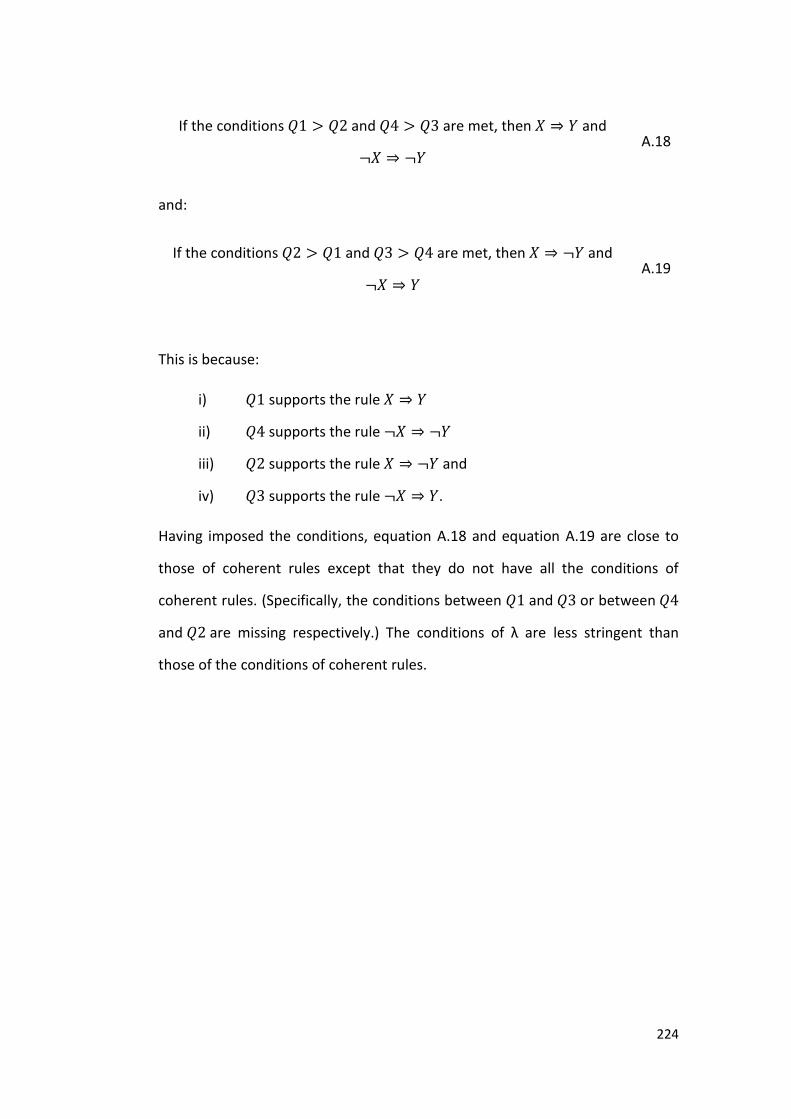
224
If the conditions 𝑄1 > 𝑄2 and 𝑄4 > 𝑄3 are met, then 𝑋 ⇒ 𝑌 and
¬𝑋 ⇒ ¬𝑌 A.18
and:
If the conditions 𝑄2 > 𝑄1 and 𝑄3 > 𝑄4 are met, then 𝑋 ⇒ ¬𝑌 and
¬𝑋 ⇒ 𝑌 A.19
This is because:
i) 𝑄1 supports the rule 𝑋 ⇒ 𝑌
ii) 𝑄4 supports the rule ¬𝑋 ⇒ ¬𝑌
iii) 𝑄2 supports the rule 𝑋 ⇒ ¬𝑌 and
iv) 𝑄3 supports the rule ¬𝑋 ⇒ 𝑌.
Having imposed the conditions, equation A.18 and equation A.19 are close to
those of coherent rules except that they do not have all the conditions of
coherent rules. (Specifically, the conditions between 𝑄1 and 𝑄3 or between 𝑄4
and 𝑄2 are missing respectively.) The conditions of λ are less stringent than
those of the conditions of coherent rules.

225
APPENDIX B
PROPERTIES OF THE
MEASURE OF
INTERESTINGNESS 𝑯
We show that the coherent rules measure of interestingness 𝐻 𝑋. .𝑌 does
not inherit the anti-monotone property. Suppose, the function 𝑆𝑉 𝑋. .𝑌 finds
all the support values of a candidate coherent rule pair such that:
𝑆𝑉 𝑋. .𝑌 = (𝑆𝑄1 𝑋. .𝑌 , 𝑆𝑄2 𝑋. .𝑌 , 𝑆𝑄3 𝑋. .𝑌 , 𝑆𝑄4 𝑋. .𝑌 ) B.1
The changes in support values between a candidate coherent rule pair and
another candidate coherent rule pair having supersets (based on Table 4-3 and
Table 4-4) is shown:
𝑆𝑉 𝑋𝐸. .𝑌 = 𝑆𝑄1 𝑋. .𝑌 − 𝛿1, 𝑆𝑄2 𝑋. .𝑌 − 𝛿2,𝑆𝑄3 𝑋. .𝑌 + 𝛿3, 𝑆𝑄4 𝑋. .𝑌 + 𝛿4
𝑤𝑒𝑟𝑒 𝛿1 + 𝛿2 = 𝛿3 + 𝛿4, (𝛿1, 𝛿2, 𝛿3, 𝛿4) ≥ 0, and 𝑋 ⊂ 𝑋𝐸
B.2

226
Based on the understanding of the delta changes in support values as
shown in equation B.2, the strength value of coherent rules written without its
conditions is as follow for 𝑚 number of transaction records based on equations
4.15, 4.12 and Table 4-3:
𝐻 𝑋. .𝑌
= 𝑚𝑖𝑛 𝑆𝑄1 𝑋..𝑌 +𝑆𝑄3 𝑋..𝑌 ,𝑚−𝑆𝑄1 𝑋..𝑌 +𝑆𝑄3 𝑋..𝑌
–𝑚𝑖𝑛 𝑆𝑄1 𝑋..𝑌 ,𝑆𝑄2 𝑋..𝑌 –𝑚𝑖𝑛 𝑆𝑄3 𝑋..𝑌 ,𝑆𝑄4 𝑋..𝑌
𝑚𝑖𝑛 𝑆𝑄1 𝑋. .𝑌 + 𝑆𝑄3 𝑋. .𝑌 ,𝑚 − 𝑆𝑄1 𝑋. .𝑌 + 𝑆𝑄3 𝑋. .𝑌
B.3
and, let the fixed value:
𝐹𝑉 = 𝑚𝑖𝑛 𝑆𝑄1 𝑋. .𝑌 + 𝑆𝑄3 𝑋. .𝑌 ,𝑚 − 𝑆𝑄1 𝑋. .𝑌 + 𝑆𝑄3 𝑋. .𝑌 B.4
(because the support values given by 𝑆𝑄1 𝑋. .𝑌 + 𝑆𝑄3 𝑋. .𝑌 is the total
number of occurrences or non occurrences for a pre-selected consequence item
set 𝑌, which is a fixed value) The equation B.3 is simplified as:
𝐻 𝑋. .𝑌 =
𝐹𝑉 − min(𝑆𝑄1 𝑋. .𝑌 , 𝑆𝑄2 𝑋. .𝑌 ),
min(𝑆𝑄3 𝑋. .𝑌 , 𝑆𝑄4 𝑋. .𝑌 )
𝐹𝑉
B.5
and, its candidate coherent rules with super item sets:
𝐻 𝑋𝐸. .𝑌 =
𝐹𝑉 − min(𝑆𝑄1 𝑋. .𝑌 − 𝛿1, 𝑆𝑄2 𝑋. .𝑌 − 𝛿2),
min(𝑆𝑄3 𝑋. .𝑌 + 𝛿3, 𝑆𝑄4 𝑋. .𝑌 + 𝛿4)
𝐹𝑉
B.6
227
If 𝛿1 and 𝛿2 are assumed zero in equation B.6, any positive values on 𝛿3 and
𝛿4 will increase the value on min(𝑆𝑄3 𝑋. .𝑌 + 𝛿3, 𝑆𝑄4 𝑋. .𝑌 + 𝛿4). As a
result, the measure of interestingness 𝐻 inhibits the anti-monotone property:
𝐻 𝑋. .𝑌 ≥ 𝐻 𝑋𝐸. .𝑌 𝑖𝑓𝑓 𝛿1 = 0, 𝛿2 = 0 B.7
On the other hand, if 𝛿3 and 𝛿4 are assumed zero in equation B.6, any positive
values on 𝛿1 and 𝛿2 will decrease the value on min(𝑆𝑄1 𝑋. .𝑌 −
𝛿1, 𝑆𝑄2 𝑋. .𝑌 − 𝛿2). As a result, the measure of interestingness 𝐻 inhibits the
monotone property:
𝐻 𝑋. .𝑌 ≤ 𝐻 𝑋𝐸. .𝑌 𝑖𝑓𝑓 𝛿3 = 0, 𝛿4 = 0 B.8
Nonetheless, both the assumptions on 𝛿1 and 𝛿2 , and 𝛿3 and 𝛿4 do not
necessarily hold. Hence, the coherent rules measure of interestingness
𝐻 𝑋𝐸. .𝑌 can be higher, lower or the same value as 𝐻 𝑋. .𝑌 .

228
APPENDIX C
DESCRIPTION OF ZOO
DATABASE
Dataset: Zoo [Fo90]
Description
Zoo dataset is a collection of animal characteristics and their classes in a
Zoo. The dataset contains 18 attributes including a class attribute. The first
attribute, animal name, is shown in the first column. This is followed by
attributes that describe an animal’s characteristics. The last class attribute
denotes an animal’s class.
Each instance uniquely describes an animal. For the purpose of mining, the
first attribute that contains the animal name will not be used. As a result, we
use the 16 attributes to describe an animal’s characteristics with the last class
attribute to show its class. Each attribute holds a value domain listed below:

229
No. Attribute Value Domain
1 animal name Unique for each instance and there are 101 types
of animals
2 hair Boolean
3 feathers Boolean
4 eggs Boolean
5 milk Boolean
6 airbone Boolean
7 aquatic Boolean
8 predator Boolean
9 toothed Boolean
10 backbone Boolean
11 breathes Boolean
12 venomous Boolean
13 fins Boolean
14 legs Numeric (set of values: {0,2,4,5,6,8})
15 tail Boolean
16 domestic Boolean
17 catsize Boolean
18 type Numeric (set of values: {1,2,3,4,5,6,7})
The last class attribute, type, holds an integer value that can be mapped to
seven different class attribute values of animals.
Class Attributes Values
The seven class attributes observed in Zoo dataset and their values are listed in
a table below:

230
Table C-1: Class Attributes in Zoo Dataset
No. Class Attribute
Class Attribute Values
Set of Animals
1 amphibian 𝑎𝑚𝑝𝑖𝑏𝑖𝑎𝑛(1);
the observe of
amphibian
frog, frog, newt, toad
(Total count : 4)
2 bird 𝑏𝑖𝑟𝑑(1) chicken, crow, dove, duck, flamingo, gull, hawk, kiwi, lark,
ostrich, parakeet, penguin, pheasant, rhea, skimmer, skua, sparrow, swan, vulture, wren
(Total count: 20)
3
fish 𝑓𝑖𝑠(1) bass, carp, catfish, chub, dogfish, haddock,
herring, pike, piranha, seahorse, sole, stingray, tuna
(Total count: 13)
4 insect 𝑖𝑛𝑠𝑒𝑐𝑡(1) flea, gnat, honeybee, housefly, ladybird, moth, termite, wasp
(Total count: 8)
5 invertebrate 𝑖𝑛𝑣𝑒𝑟𝑡𝑒𝑏𝑟𝑎𝑡𝑒(1) clam, crab, crayfish, lobster, octopus, scorpion, seawasp,
slug, starfish, worm
(Total count: 10)
6 mammal 𝑚𝑎𝑚𝑚𝑎𝑙(1) aardvark, antelope, bear, boar, buffalo, calf, cavy, cheetah,
deer, dolphin, elephant, fruitbat, giraffe, girl, goat,
gorilla, hamster, hare, leopard, lion, lynx, mink,
mole, mongoose, opossum, oryx, platypus,
polecat, pony, porpoise, puma, pussycat,
raccoon, reindeer, seal, sealion, squirrel, vampire,
vole, wallaby,wolf
(Total count: 41)
7 reptile 𝑟𝑒𝑝𝑡𝑖𝑙𝑒(1) pitviper, seasnake, slowworm, tortoise, tuatara
(Total count: 5)

231
Attributes Values (excluding the Class Attribute)
Among the 16 attributes, only one attribute, leg, has multiple values. The other
attributes hold a value ‘1’ to denote the presence (observed) of an attribute. All
the attribute values are listed in a table below:
Table C-2: Attributes and Their Attribute Values in Zoo Dataset
No. Attribute Attribute Values
1 Hair 𝑎𝑖𝑟(1); “the presence of hair as part of the characteristic of an animal”
2 Feathers 𝑓𝑒𝑎𝑡𝑒𝑟𝑠(1); “the presence of feathers”
3 Eggs 𝑒𝑔𝑔𝑠(1)
4 Milk 𝑚𝑖𝑙𝑘(1)
5 Airborne 𝑎𝑖𝑟𝑏𝑜𝑟𝑛𝑒(1)
6 Aquatic 𝑎𝑞𝑢𝑎𝑡𝑖𝑐(1)
7 predator 𝑝𝑟𝑒𝑑𝑎𝑡𝑜𝑟(1)
8 Toothed 𝑡𝑜𝑜𝑡𝑒𝑑(1)
9 backbone 𝑏𝑎𝑐𝑘𝑏𝑜𝑛𝑒(1)
10 breathes 𝑏𝑟𝑒𝑎𝑡𝑒𝑠(1)
11 venomous 𝑣𝑒𝑛𝑜𝑚𝑜𝑢𝑠(1)
12 fins 𝑓𝑖𝑛𝑠(1)
13 legs 𝑙𝑒𝑔𝑠(0), 𝑙𝑒𝑔𝑠(2), 𝑙𝑒𝑔𝑠(4), 𝑙𝑒𝑔𝑠(5), 𝑙𝑒𝑔𝑠(6), 𝑙𝑒𝑔𝑠(8)
14 tail 𝑡𝑎𝑖𝑙(1)
15 domestic 𝑑𝑜𝑚𝑒𝑠𝑡𝑖𝑐(1)
16 catsize 𝑐𝑎𝑡𝑠𝑖𝑧𝑒(1)
Total 16 attributes
21 attribute values
Instances: Zoo dataset has 101 instances (or lines) of transaction records.

232
APPENDIX D
ASSOCIATION RULES
FOUND ON INFREQUENTLY
OBSERVED CLASS VALUES

233
All
cohe
rent
rul
es fo
und
usin
g 𝐸𝑆𝑆
_𝐶𝑅
for
the
attr
ibut
e va
lue
Rep
tile
(1)
No
Ant
.1
Ant
.2
Ant
.3
Ant
.4
Ant
.5
Ant
.6
Ant
.7
Conq
Su
p1
Conf
1 Su
p2
Conf
2
Num
ber
of
Item
s on
A
nt
1
eggs
(1)
toot
hed(
1)
brea
thes
(1)
tail(
1)
Rep
tile
(1)
3%
75%
94
%
98%
4
2
eg
gs(1
) pr
edat
or(1
) to
othe
d(1)
br
eath
es(1
) ta
il(1)
R
epti
le(1
) 3%
75
%
94%
98
%
5
3
eg
gs(1
) to
othe
d(1)
ba
ckbo
ne(1
) br
eath
es(1
) ta
il(1)
R
epti
le(1
) 3%
75
%
94%
98
%
5
4
pr
edat
or(1
) to
othe
d(1)
ba
ckbo
ne(1
) br
eath
es(1
) ta
il(1)
R
epti
le(1
) 3%
75
%
94%
98
%
5

234
All
cohe
rent
rul
es fo
und
usin
g 𝐸𝑆𝑆
_𝐶𝑅
for
the
att
ribu
te v
alue
Am
pbib
ian(
1)
No
A
nt.1
A
nt.2
A
nt.3
A
nt.4
A
nt.5
A
nt.6
A
nt.7
C
onq
Sup1
C
onf1
Su
p2
Con
f2
Num
ber
of
Item
s o
n A
nt
1
aqua
tic(
1)
legs
(4)
Am
phib
ian(
1)
4%
57%
93
%
100%
2
2
eg
gs(1
) to
oth
ed(1
) br
eath
es(1
) A
mph
ibia
n(1)
4%
57
%
93%
10
0%
3
3
eg
gs(1
) aq
uati
c(1)
le
gs(4
) A
mph
ibia
n(1)
4%
67
%
94%
10
0%
3
4
eg
gs(1
) to
oth
ed(1
) le
gs(4
) A
mph
ibia
n(1)
4%
80
%
95%
10
0%
3
5
aq
uati
c(1)
to
oth
ed(1
) le
gs(4
) A
mph
ibia
n(1)
4%
80
%
95%
10
0%
3
6
eg
gs(1
) ba
ckbo
ne(1
) le
gs(4
) A
mph
ibia
n(1)
4%
57
%
93%
10
0%
3
7
aq
uati
c(1)
ba
ckbo
ne(1
) le
gs(4
) A
mph
ibia
n(1)
4%
67
%
94%
10
0%
3
8
eg
gs(1
) br
eath
es(1
) le
gs(4
) A
mph
ibia
n(1)
4%
57
%
93%
10
0%
3
9
aq
uati
c(1)
br
eath
es(1
) le
gs(4
) A
mph
ibia
n(1)
4%
67
%
94%
10
0%
3
10
eg
gs(1
) aq
uati
c(1)
to
oth
ed(1
) br
eath
es(1
) A
mph
ibia
n(1)
4%
10
0%
96%
10
0%
4
11
eg
gs(1
) to
oth
ed(1
) ba
ckbo
ne(1
) br
eath
es(1
) A
mph
ibia
n(1)
4%
57
%
93%
10
0%
4
12
eg
gs(1
) aq
uati
c(1)
pr
edat
or(
1)
legs
(4)
Am
phib
ian(
1)
3%
60%
94
%
99%
4
13
eg
gs(1
) aq
uati
c(1)
to
oth
ed(1
) le
gs(4
) A
mph
ibia
n(1)
4%
10
0%
96%
10
0%
4
14
eg
gs(1
) pr
edat
or(
1)
too
thed
(1)
legs
(4)
Am
phib
ian(
1)
3%
75%
95
%
99%
4
15
aq
uati
c(1)
pr
edat
or(
1)
too
thed
(1)
legs
(4)
Am
phib
ian(
1)
3%
75%
95
%
99%
4
16
eg
gs(1
) aq
uati
c(1)
ba
ckbo
ne(1
) le
gs(4
) A
mph
ibia
n(1)
4%
80
%
95%
10
0%
4
17
eg
gs(1
) pr
edat
or(
1)
back
bone
(1)
legs
(4)
Am
phib
ian(
1)
3%
60%
94
%
99%
4
18
aq
uati
c(1)
pr
edat
or(
1)
back
bone
(1)
legs
(4)
Am
phib
ian(
1)
3%
60%
94
%
99%
4
19
eg
gs(1
) to
oth
ed(1
) ba
ckbo
ne(1
) le
gs(4
) A
mph
ibia
n(1)
4%
80
%
95%
10
0%
4
20
aq
uati
c(1)
to
oth
ed(1
) ba
ckbo
ne(1
) le
gs(4
) A
mph
ibia
n(1)
4%
80
%
95%
10
0%
4
21
eg
gs(1
) aq
uati
c(1)
br
eath
es(1
) le
gs(4
) A
mph
ibia
n(1)
4%
80
%
95%
10
0%
4
22
eg
gs(1
) pr
edat
or(
1)
brea
thes
(1)
legs
(4)
Am
phib
ian(
1)
3%
60%
94
%
99%
4
23
aq
uati
c(1)
pr
edat
or(
1)
brea
thes
(1)
legs
(4)
Am
phib
ian(
1)
3%
60%
94
%
99%
4
24
eg
gs(1
) to
oth
ed(1
) br
eath
es(1
) le
gs(4
) A
mph
ibia
n(1)
4%
80
%
95%
10
0%
4
25
aqua
tic(
1)
too
thed
(1)
brea
thes
(1)
legs
(4)
Am
phib
ian(
1)
4%
80%
95
%
100%
4

235
No
Ant
.1
Ant
.2
Ant
.3
Ant
.4
Ant
.5
Ant
.6
Ant
.7
Conq
Su
p1
Conf
1 Su
p2
Conf
2
Num
ber
of
Item
s on
A
nt
26
eg
gs(1
) ba
ckbo
ne(1
) br
eath
es(1
) le
gs(4
) A
mph
ibia
n(1)
4%
57
%
93%
10
0%
4
27
aq
uati
c(1)
ba
ckbo
ne(1
) br
eath
es(1
) le
gs(4
) A
mph
ibia
n(1)
4%
67
%
94%
10
0%
4
28
eggs
(1)
aqua
tic(
1)
pred
ator
(1)
toot
hed(
1)
brea
thes
(1)
Am
phib
ian(
1)
3%
100%
96
%
99%
5
29
eggs
(1)
aqua
tic(
1)
toot
hed(
1)
back
bone
(1)
brea
thes
(1)
Am
phib
ian(
1)
4%
100%
96
%
100%
5
30
eggs
(1)
aqua
tic(
1)
pred
ator
(1)
toot
hed(
1)
legs
(4)
Am
phib
ian(
1)
3%
100%
96
%
99%
5
31
eggs
(1)
aqua
tic(
1)
pred
ator
(1)
back
bone
(1)
legs
(4)
Am
phib
ian(
1)
3%
75%
95
%
99%
5
32
eggs
(1)
aqua
tic(
1)
toot
hed(
1)
back
bone
(1)
legs
(4)
Am
phib
ian(
1)
4%
100%
96
%
100%
5
33
eggs
(1)
pred
ator
(1)
toot
hed(
1)
back
bone
(1)
legs
(4)
Am
phib
ian(
1)
3%
75%
95
%
99%
5
34
aqua
tic(
1)
pred
ator
(1)
toot
hed(
1)
back
bone
(1)
legs
(4)
Am
phib
ian(
1)
3%
75%
95
%
99%
5
35
eggs
(1)
aqua
tic(
1)
pred
ator
(1)
brea
thes
(1)
legs
(4)
Am
phib
ian(
1)
3%
75%
95
%
99%
5
36
eggs
(1)
aqua
tic(
1)
toot
hed(
1)
brea
thes
(1)
legs
(4)
Am
phib
ian(
1)
4%
100%
96
%
100%
5
37
eggs
(1)
pred
ator
(1)
toot
hed(
1)
brea
thes
(1)
legs
(4)
Am
phib
ian(
1)
3%
75%
95
%
99%
5
38
aqua
tic(
1)
pred
ator
(1)
toot
hed(
1)
brea
thes
(1)
legs
(4)
Am
phib
ian(
1)
3%
75%
95
%
99%
5
39
eggs
(1)
aqua
tic(
1)
back
bone
(1)
brea
thes
(1)
legs
(4)
Am
phib
ian(
1)
4%
80%
95
%
100%
5
40
eggs
(1)
pred
ator
(1)
back
bone
(1)
brea
thes
(1)
legs
(4)
Am
phib
ian(
1)
3%
60%
94
%
99%
5
41
aqua
tic(
1)
pred
ator
(1)
back
bone
(1)
brea
thes
(1)
legs
(4)
Am
phib
ian(
1)
3%
60%
94
%
99%
5
42
eggs
(1)
toot
hed(
1)
back
bone
(1)
brea
thes
(1)
legs
(4)
Am
phib
ian(
1)
4%
80%
95
%
100%
5
43
aqua
tic(
1)
toot
hed(
1)
back
bone
(1)
brea
thes
(1)
legs
(4)
Am
phib
ian(
1)
4%
80%
95
%
100%
5
44
eg
gs(1
) aq
uati
c(1)
pr
edat
or(1
) to
othe
d(1)
ba
ckbo
ne(1
) br
eath
es(1
) A
mph
ibia
n(1)
3%
10
0%
96%
99
%
6
45
eg
gs(1
) aq
uati
c(1)
pr
edat
or(1
) to
othe
d(1)
ba
ckbo
ne(1
) le
gs(4
) A
mph
ibia
n(1)
3%
10
0%
96%
99
%
6
46
eg
gs(1
) aq
uati
c(1)
pr
edat
or(1
) to
othe
d(1)
br
eath
es(1
) le
gs(4
) A
mph
ibia
n(1)
3%
10
0%
96%
99
%
6
47
eg
gs(1
) aq
uati
c(1)
pr
edat
or(1
) ba
ckbo
ne(1
) br
eath
es(1
) le
gs(4
) A
mph
ibia
n(1)
3%
75
%
95%
99
%
6
48
eg
gs(1
) aq
uati
c(1)
to
othe
d(1)
ba
ckbo
ne(1
) br
eath
es(1
) le
gs(4
) A
mph
ibia
n(1)
4%
10
0%
96%
10
0%
6
49
eg
gs(1
) pr
edat
or(1
) to
othe
d(1)
ba
ckbo
ne(1
) br
eath
es(1
) le
gs(4
) A
mph
ibia
n(1)
3%
75
%
95%
99
%
6
50
aq
uati
c(1)
pr
edat
or(1
) to
othe
d(1)
ba
ckbo
ne(1
) br
eath
es(1
) le
gs(4
) A
mph
ibia
n(1)
3%
75
%
95%
99
%
6
51
eggs
(1)
aqua
tic(
1)
pred
ator
(1)
toot
hed(
1)
back
bone
(1)
brea
thes
(1)
legs
(4)
Am
phib
ian(
1)
3%
100%
96
%
99%
7

236
APPENDIX E
RESIDUALS AT VARYING
LENGTH WINDOW 𝑳
This appendix shows the number of residuals after each constraint on the Zoo
dataset (Appendix C),
(i) 𝐶1: 𝐻′′ ≤ 𝑚𝑖𝑛_,
(ii) 𝐶2: 𝐻′ ≤ 𝑚𝑖𝑛_,
(iii) 𝐶3: 𝑆𝑄1 𝒳. .𝒴 > 𝑆𝑄3 𝒳. .𝒴 , and
(iv) 𝐶4: 𝑠𝑧 𝒳. .𝒴 ≤ 𝑚𝑎𝑥_𝑠𝑧
All strength values of coherent rules are allowed to be discovered (i.e. the
parameter value 𝑊 is set to be 1). The indicators used are as below:
a - number of coherent rules that passes a constraint,
b - number of coherent rules discovered,
c - residuals of a constraint,
d - percentage of ‘c' over ‘a’

237
The residual of a constraint (‘c’) is calculated as the number of coherent rules
that passes a constraint (‘a’) minus the number of coherent rules discovered
(‘b’) following equation 5.1. And, the number of residuals in percentage is given
by (‘d’) following equation 5.2.

238
Table E-1: The Residuals at varying Parameter 𝐿 (𝑌 = {′𝑟𝑒𝑝𝑡𝑖𝑙𝑒′}, 1st Phase)
a b H''≤min_h H'≤min_h SQ1(X..Y)>SQ3(X..Y)
c d
0 101 1 101 1 73 1
100 99.0% 100 99.0% 72 98.6%
2 111 4 111 4 79 4
107 96.4% 107 96.4% 75 94.9%
4 111 4 111 4 79 4
107 96.4% 107 96.4% 75 94.9%
6 111 4 111 4 79 4
107 96.4% 107 96.4% 75 94.9%
8 111 4 111 4 79 4
107 96.4% 107 96.4% 75 94.9%
10 111 4 111 4 79 4
107 96.4% 107 96.4% 75 94.9%
12 111 4 111 4 79 4
107 96.4% 107 96.4% 75 94.9%
14 111 4 111 4 79 4
107 96.4% 107 96.4% 75 94.9%
16 111 4 111 4 79 4
107 96.4% 107 96.4% 75 94.9%
Table E-2: The Residuals at varying Parameter 𝐿 (𝑌 = {′𝑟𝑒𝑝𝑡𝑖𝑙𝑒′}, 2nd Phase)
a b H''≤min_h H'≤min_h SQ1(X..Y)>SQ3(X..Y)
c d
0 51 0 51 0 11 0
51 100.0% 51 100.0% 11 100.0%
2 51 0 51 0 11 0
51 100.0% 51 100.0% 11 100.0%
4 51 0 51 0 11 0
51 100.0% 51 100.0% 11 100.0%
6 51 0 51 0 11 0
51 100.0% 51 100.0% 11 100.0%
8 51 0 51 0 11 0
51 100.0% 51 100.0% 11 100.0%
10 51 0 51 0 11 0
51 100.0% 51 100.0% 11 100.0%
12 51 0 51 0 11 0
51 100.0% 51 100.0% 11 100.0%
14 51 0 51 0 11 0
51 100.0% 51 100.0% 11 100.0%
16 51 0 51 0 11 0
51 100.0% 51 100.0% 11 100.0%

239
Table E-3: The Residuals at varying Parameter 𝐿 (𝑌 = {′𝑚𝑎𝑚𝑚𝑎𝑙′}, 1st Phase)
a b H''≤min_h H'≤min_h SQ1(X..Y)>SQ3(X..Y)
c d
0 21 5 21 5 9 5
16 76.2% 16 76.2% 4 44.4%
2 135 97 135 97 103 97
38 28.1% 38 28.1% 6 5.8%
4 310 228 310 228 234 228
82 26.5% 82 26.5% 6 2.6%
6 354 264 354 264 270 264
90 25.4% 90 25.4% 6 2.2%
8 355 265 355 265 271 265
90 25.4% 90 25.4% 6 2.2%
10 355 265 355 265 271 265
90 25.4% 90 25.4% 6 2.2%
12 355 265 355 265 271 265
90 25.4% 90 25.4% 6 2.2%
14 355 265 355 265 271 265
90 25.4% 90 25.4% 6 2.2%
16 355 265 355 265 271 265
90 25.4% 90 25.4% 6 2.2%
Table E-4: The Residuals at varying Parameter 𝐿 (𝑌 = {′𝑚𝑎𝑚𝑚𝑎𝑙′}, 2nd Phase)
a b H''≤min_h H'≤min_h SQ1(X..Y)>SQ3(X..Y)
c d
0 21 1 21 1 5 1
20 95.2% 20 95.2% 4 80.0%
2 33 6 33 6 11 6
27 81.8% 27 81.8% 5 45.5%
4 33 6 33 6 11 6
27 81.8% 27 81.8% 5 45.5%
6 33 6 33 6 11 6
27 81.8% 27 81.8% 5 45.5%
8 33 6 33 6 11 6
27 81.8% 27 81.8% 5 45.5%
10 33 6 33 6 11 6
27 81.8% 27 81.8% 5 45.5%
12 33 6 33 6 11 6
27 81.8% 27 81.8% 5 45.5%
14 33 6 33 6 11 6
27 81.8% 27 81.8% 5 45.5%
16 33 6 33 6 11 6
27 81.8% 27 81.8% 5 45.5%

240
Table E-5: The Residuals at varying Parameter 𝐿 (𝑌 = {′ 𝑖𝑛𝑣𝑒𝑟𝑡𝑒𝑏𝑟. ′}, 1st Phase)
a b H''≤min_h H'≤min_h SQ1(X..Y)>SQ3(X..Y)
c d
0 25 0 25 0 7 0
25 100.0% 25 100.0% 7 100.0%
2 25 0 25 0 7 0
25 100.0% 25 100.0% 7 100.0%
4 25 0 25 0 7 0
25 100.0% 25 100.0% 7 100.0%
6 25 0 25 0 7 0
25 100.0% 25 100.0% 7 100.0%
8 25 0 25 0 7 0
25 100.0% 25 100.0% 7 100.0%
10 25 0 25 0 7 0
25 100.0% 25 100.0% 7 100.0%
12 25 0 25 0 7 0
25 100.0% 25 100.0% 7 100.0%
14 25 0 25 0 7 0
25 100.0% 25 100.0% 7 100.0%
16 25 0 25 0 7 0
25 100.0% 25 100.0% 7 100.0%
Table E-6: The Residuals at varying Parameter 𝐿 (𝑌 = {′ 𝑖𝑛𝑣𝑒𝑟𝑡𝑒𝑏𝑟. ′}, 2nd Phase)
a b H''≤min_h H'≤min_h SQ1(X..Y)>SQ3(X..Y)
c d
0 24 1 24 1 6 1
23 95.8% 23 95.8% 5 83.3%
2 53 1 53 1 16 1
52 98.1% 52 98.1% 15 93.8%
4 60 1 60 1 16 1
59 98.3% 59 98.3% 15 93.8%
6 60 1 60 1 16 1
59 98.3% 59 98.3% 15 93.8%
8 60 1 60 1 16 1
59 98.3% 59 98.3% 15 93.8%
10 60 1 60 1 16 1
59 98.3% 59 98.3% 15 93.8%
12 60 1 60 1 16 1
59 98.3% 59 98.3% 15 93.8%
14 60 1 60 1 16 1
59 98.3% 59 98.3% 15 93.8%
16 60 1 60 1 16 1
59 98.3% 59 98.3% 15 93.8%

241
Table E-7: The Residuals at varying Parameter 𝐿 (𝑌 = {′𝑖𝑛𝑠𝑒𝑐𝑡′}, 1st Phase)
a b H''≤min_h H'≤min_h SQ1(X..Y)>SQ3(X..Y)
c d
0 25 1 25 1 8 1
24 96.0% 24 96.0% 7 87.5%
2 31 7 31 7 14 7
24 77.4% 24 77.4% 7 50.0%
4 32 8 32 8 15 8
24 75.0% 24 75.0% 7 46.7%
6 32 8 32 8 15 8
24 75.0% 24 75.0% 7 46.7%
8 32 8 32 8 15 8
24 75.0% 24 75.0% 7 46.7%
10 32 8 32 8 15 8
24 75.0% 24 75.0% 7 46.7%
12 32 8 32 8 15 8
24 75.0% 24 75.0% 7 46.7%
14 32 8 32 8 15 8
24 75.0% 24 75.0% 7 46.7%
16 32 8 32 8 15 8
24 75.0% 24 75.0% 7 46.7%
Table E-8: The Residuals at varying Parameter 𝐿 (𝑌 = {′𝑖𝑛𝑠𝑒𝑐𝑡′}, 2nd Phase)
a b H''≤min_h H'≤min_h SQ1(X..Y)>SQ3(X..Y)
c d
0 60 0 60 0 16 0
60 100.0% 60 100.0% 16 100.0%
2 60 0 60 0 16 0
60 100.0% 60 100.0% 16 100.0%
4 60 0 60 0 16 0
60 100.0% 60 100.0% 16 100.0%
6 60 0 60 0 16 0
60 100.0% 60 100.0% 16 100.0%
8 60 0 60 0 16 0
60 100.0% 60 100.0% 16 100.0%
10 60 0 60 0 16 0
60 100.0% 60 100.0% 16 100.0%
12 60 0 60 0 16 0
60 100.0% 60 100.0% 16 100.0%
14 60 0 60 0 16 0
60 100.0% 60 100.0% 16 100.0%
16 60 0 60 0 16 0
60 100.0% 60 100.0% 16 100.0%

242
Table E-9: The Residuals at varying Parameter 𝐿 (𝑌 = {′𝑓𝑖𝑠′), 1st Phase)
a b H''≤min_h H'≤min_h SQ1(X..Y)>SQ3(X..Y)
c d
0 32 2 32 2 19 2
30 93.8% 30 93.8% 17 89.5%
2 175 127 175 127 162 127
48 27.4% 48 27.4% 35 21.6%
4 259 211 259 211 246 211
48 18.5% 48 18.5% 35 14.2%
6 268 220 268 220 255 220
48 17.9% 48 17.9% 35 13.7%
8 268 220 268 220 255 220
48 17.9% 48 17.9% 35 13.7%
10 268 220 268 220 255 220
48 17.9% 48 17.9% 35 13.7%
12 268 220 268 220 255 220
48 17.9% 48 17.9% 35 13.7%
14 268 220 268 220 255 220
48 17.9% 48 17.9% 35 13.7%
16 268 220 268 220 255 220
48 17.9% 48 17.9% 35 13.7%
Table E-10: The Residuals at varying Parameter 𝐿 (𝑌 = {′𝑓𝑖𝑠′}, 2nd Phase)
a b H''≤min_h H'≤min_h SQ1(X..Y)>SQ3(X..Y)
c d
0 29 1 29 1 7 1
28 96.6% 28 96.6% 6 85.7%
2 50 1 50 1 13 1
49 98.0% 49 98.0% 12 92.3%
4 55 1 55 1 13 1
54 98.2% 54 98.2% 12 92.3%
6 55 1 55 1 13 1
54 98.2% 54 98.2% 12 92.3%
8 55 1 55 1 13 1
54 98.2% 54 98.2% 12 92.3%
10 55 1 55 1 13 1
54 98.2% 54 98.2% 12 92.3%
12 55 1 55 1 13 1
54 98.2% 54 98.2% 12 92.3%
14 55 1 55 1 13 1
54 98.2% 54 98.2% 12 92.3%
16 55 1 55 1 13 1
54 98.2% 54 98.2% 12 92.3%

243
Table E-11: The Residuals at varying Parameter 𝐿 (𝑌 = {′𝑏𝑖𝑟𝑑′}, 1st Phase)
a b H''≤min_h H'≤min_h SQ1(X..Y)>SQ3(X..Y)
c d
0 21 3 21 3 7 3
18 85.7% 18 85.7% 4 57.1%
2 77 54 77 54 63 54
23 29.9% 23 29.9% 9 14.3%
4 133 110 133 110 119 110
23 17.3% 23 17.3% 9 7.6%
6 141 118 141 118 127 118
23 16.3% 23 16.3% 9 7.1%
8 141 118 141 118 127 118
23 16.3% 23 16.3% 9 7.1%
10 141 118 141 118 127 118
23 16.3% 23 16.3% 9 7.1%
12 141 118 141 118 127 118
23 16.3% 23 16.3% 9 7.1%
14 141 118 141 118 127 118
23 16.3% 23 16.3% 9 7.1%
16 141 118 141 118 127 118
23 16.3% 23 16.3% 9 7.1%
Table E-12: The Residuals at varying Parameter 𝐿 (𝑌 = {′𝑏𝑖𝑟𝑑′}, 2nd Phase)
a b H''≤min_h H'≤min_h SQ1(X..Y)>SQ3(X..Y)
c d
0 73 0 73 0 19 0
73 100.0% 73 100.0% 19 100.0%
2 73 0 73 0 19 0
73 100.0% 73 100.0% 19 100.0%
4 73 0 73 0 19 0
73 100.0% 73 100.0% 19 100.0%
6 73 0 73 0 19 0
73 100.0% 73 100.0% 19 100.0%
8 73 0 73 0 19 0
73 100.0% 73 100.0% 19 100.0%
10 73 0 73 0 19 0
73 100.0% 73 100.0% 19 100.0%
12 73 0 73 0 19 0
73 100.0% 73 100.0% 19 100.0%
14 73 0 73 0 19 0
73 100.0% 73 100.0% 19 100.0%
16 73 0 73 0 19 0
73 100.0% 73 100.0% 19 100.0%

244
Table E-13: The Residuals at varying Parameter 𝐿 (𝑌 = {′𝑎𝑚𝑝𝑖𝑏𝑛. ′}, 1st Phase)
a b H''≤min_h H'≤min_h SQ1(X..Y)>SQ3(X..Y)
c d
0 69 1 69 1 55 1
68 98.6% 68 98.6% 54 98.2%
2 133 43 133 43 119 43
90 67.7% 90 67.7% 76 63.9%
4 141 51 141 51 127 51
90 63.8% 90 63.8% 76 59.8%
6 141 51 141 51 127 51
90 63.8% 90 63.8% 76 59.8%
8 141 51 141 51 127 51
90 63.8% 90 63.8% 76 59.8%
10 141 51 141 51 127 51
90 63.8% 90 63.8% 76 59.8%
12 141 51 141 51 127 51
90 63.8% 90 63.8% 76 59.8%
14 141 51 141 51 127 51
90 63.8% 90 63.8% 76 59.8%
16 141 51 141 51 127 51
90 63.8% 90 63.8% 76 59.8%
Table E-14: The Residuals at varying Parameter 𝐿 (𝑌 = {′𝑎𝑚𝑝𝑖𝑏𝑛. ′}, 2nd Phase)
a b H''≤min_h H'≤min_h SQ1(X..Y)>SQ3(X..Y)
c d
0 55 0 55 0 13 0
55 100.0% 55 100.0% 13 100.0%
2 55 0 55 0 13 0
55 100.0% 55 100.0% 13 100.0%
4 55 0 55 0 13 0
55 100.0% 55 100.0% 13 100.0%
6 55 0 55 0 13 0
55 100.0% 55 100.0% 13 100.0%
8 55 0 55 0 13 0
55 100.0% 55 100.0% 13 100.0%
10 55 0 55 0 13 0
55 100.0% 55 100.0% 13 100.0%
12 55 0 55 0 13 0
55 100.0% 55 100.0% 13 100.0%
14 55 0 55 0 13 0
55 100.0% 55 100.0% 13 100.0%
16 55 0 55 0 13 0
55 100.0% 55 100.0% 13 100.0%

245
APPENDIX F
RESIDUALS AT VARYING
STRENGTH VALUE
WINDOW 𝑾
This appendix shows the number of residuals after each constraint on the
Zoo dataset (Appendix C),
(v) 𝐶1: 𝐻′′ ≤ 𝑚𝑖𝑛_,
(vi) 𝐶2: 𝐻′ ≤ 𝑚𝑖𝑛_,
(vii) 𝐶3: 𝑆𝑄1 𝒳. .𝒴 > 𝑆𝑄3 𝒳. .𝒴 , and
(viii) 𝐶4: 𝑠𝑧 𝒳. .𝒴 ≤ 𝑚𝑎𝑥_𝑠𝑧
All sizes of coherent rules are allowed to be discovered (i.e. the parameter value
𝐿 is set to be 16). The indicators used are as below:
a - number of coherent rules that passes a constraint,
b - number of coherent rules discovered,
c - residuals of a constraint,
d - percentage of ‘c' over ‘a’

246
The residual of a constraint (‘c’) is calculated as the number of coherent rules
that passes a constraint (‘a’) minus the number of coherent rules discovered
(‘b’) following equation 5.1. And, the number of residuals in percentage is given
by (‘d’) following equation 5.2.

247
Table F-1: The Residuals at varying Parameter 𝑊 (𝑌 = {′𝑟𝑒𝑝𝑡𝑖𝑙𝑒′}, 1st Phase)
a b H''≤min_h H'≤min_h SQ1(X..Y)>SQ3(X..Y)
c d
0 111 4 111 4 79 4
107 96.4% 107 96.4% 75 94.9%
0.2 111 4 111 4 79 4
107 96.4% 107 96.4% 75 94.9%
0.4 111 4 111 4 79 4
107 96.4% 107 96.4% 75 94.9%
0.6 111 4 111 4 79 4
107 96.4% 107 96.4% 75 94.9%
0.8 111 4 111 4 79 4
107 96.4% 107 96.4% 75 94.9%
1 111 4 111 4 79 4
107 96.4% 107 96.4% 75 94.9%
Table F-2: The Residuals at varying Parameter 𝑊 (𝑌 = {′𝑟𝑒𝑝𝑡𝑖𝑙𝑒′}, 2nd Phase)
a b H''≤min_h H'≤min_h SQ1(X..Y)>SQ3(X..Y)
c d
0 51 0 51 0 11 0
51 100.0% 51 100.0% 11 100.0%
0.2 51 0 51 0 11 0
51 100.0% 51 100.0% 11 100.0%
0.4 51 0 51 0 11 0
51 100.0% 51 100.0% 11 100.0%
0.6 51 0 51 0 11 0
51 100.0% 51 100.0% 11 100.0%
0.8 51 0 51 0 11 0
51 100.0% 51 100.0% 11 100.0%
1 51 0 51 0 11 0
51 100.0% 51 100.0% 11 100.0%

248
Table F-3: The Residuals at varying Parameter 𝑊 (𝑌 = {′𝑚𝑎𝑚𝑚𝑎𝑙′}, 1st Phase)
a b H''≤min_h H'≤min_h SQ1(X..Y)>SQ3(X..Y)
c d
0 32 4 8 4 8 4
28 87.5% 4 50.0% 4 50.0%
0.2 78 42 55 42 55 42
36 46.2% 13 23.6% 13 23.6%
0.4 225 175 199 175 199 175
50 22.2% 24 12.1% 24 12.1%
0.6 355 252 271 252 271 252
103 29.0% 19 7.0% 19 7.0%
0.8 355 261 271 261 271 261
94 26.5% 10 3.7% 10 3.7%
1 355 265 355 265 271 265
90 25.4% 90 25.4% 6 2.2%
Table F-4: The Residuals at varying Parameter 𝑊 (𝑌 = {′𝑚𝑎𝑚𝑚𝑎𝑙′}, 2nd Phase)
a b H''≤min_h H'≤min_h SQ1(X..Y)>SQ3(X..Y)
c d
0 21 1 3 1 1 1
20 95.2% 2 66.7% 0 0.0%
0.2 21 1 3 1 1 1
20 95.2% 2 66.7% 0 0.0%
0.4 22 1 4 1 2 1
21 95.5% 3 75.0% 1 50.0%
0.6 28 5 11 5 9 5
23 82.1% 6 54.5% 4 44.4%
0.8 33 6 13 6 11 6
27 81.8% 7 53.8% 5 45.5%
1 33 6 33 6 11 6
27 81.8% 27 81.8% 5 45.5%

249
Table F-5: The Residuals at varying Parameter W (Y = {′ 𝑖𝑛𝑣𝑒𝑟𝑡𝑒𝑏𝑟𝑎𝑡𝑒′}, 1st
Phase)
a b H''≤min_h H'≤min_h SQ1(X..Y)>SQ3(X..Y)
c d
0 25 0 25 0 7 0
25 100.0% 25 100.0% 7 100.0%
0.2 25 0 25 0 7 0
25 100.0% 25 100.0% 7 100.0%
0.4 25 0 25 0 7 0
25 100.0% 25 100.0% 7 100.0%
0.6 25 0 25 0 7 0
25 100.0% 25 100.0% 7 100.0%
0.8 25 0 25 0 7 0
25 100.0% 25 100.0% 7 100.0%
1 25 0 25 0 7 0
25 100.0% 25 100.0% 7 100.0%
Table F-6: The Residuals at varying Parameter 𝑊 (𝑌 = {′𝑖𝑛𝑣𝑒𝑟𝑡𝑒𝑏𝑟𝑎𝑡𝑒′}, 2nd
Phase)
a b H''≤min_h H'≤min_h SQ1(X..Y)>SQ3(X..Y)
c d
0 27 1 12 1 4 1
26 96.3% 11 91.7% 3 75.0%
0.2 27 1 12 1 4 1
26 96.3% 11 91.7% 3 75.0%
0.4 27 1 12 1 4 1
26 96.3% 11 91.7% 3 75.0%
0.6 27 1 12 1 4 1
26 96.3% 11 91.7% 3 75.0%
0.8 27 1 12 1 4 1
26 96.3% 11 91.7% 3 75.0%
1 60 1 60 1 16 1
59 98.3% 59 98.3% 15 93.8%

250
Table F-7: The Residuals at varying Parameter W (Y = {′𝑖𝑛𝑠𝑒𝑐𝑡′}, 1st Phase)
a b H''≤min_h H'≤min_h SQ1(X..Y)>SQ3(X..Y)
c d
0 31 2 26 2 13 2
29 93.5% 24 92.3% 11 84.6%
0.2 31 2 26 2 13 2
29 93.5% 24 92.3% 11 84.6%
0.4 32 8 28 8 15 8
24 75.0% 20 71.4% 7 46.7%
0.6 32 8 28 8 15 8
24 75.0% 20 71.4% 7 46.7%
0.8 32 8 28 8 15 8
24 75.0% 20 71.4% 7 46.7%
1 32 8 32 8 15 8
24 75.0% 24 75.0% 7 46.7%
Table F-8: The Residuals at varying Parameter 𝑊 (𝑌 = {′𝑖𝑛𝑠𝑒𝑐𝑡′}, 2nd Phase)
a b H''≤min_h H'≤min_h SQ1(X..Y)>SQ3(X..Y)
c d
0 60 0 60 0 16 0
60 100.0% 60 100.0% 16 100.0%
0.2 60 0 60 0 16 0
60 100.0% 60 100.0% 16 100.0%
0.4 60 0 60 0 16 0
60 100.0% 60 100.0% 16 100.0%
0.6 60 0 60 0 16 0
60 100.0% 60 100.0% 16 100.0%
0.8 60 0 60 0 16 0
60 100.0% 60 100.0% 16 100.0%
1 60 0 60 0 16 0
60 100.0% 60 100.0% 16 100.0%

251
Table F-9: The Residuals at varying Parameter 𝑊 (𝑌 = {′𝑓𝑖𝑠′), 1st Phase)
a b H''≤min_h H'≤min_h SQ1(X..Y)>SQ3(X..Y)
c d
0 187 39 160 39 147 39
148 79.1% 121 75.6% 108 73.5%
0.2 187 57 160 57 147 57
130 69.5% 103 64.4% 90 61.2%
0.4 268 139 268 139 255 139
129 48.1% 129 48.1% 116 45.5%
0.6 268 184 268 184 255 184
84 31.3% 84 31.3% 71 27.8%
0.8 268 217 268 217 255 217
51 19.0% 51 19.0% 38 14.9%
1 268 220 268 220 255 220
48 17.9% 48 17.9% 35 13.7%
Table F-10: The Residuals at varying Parameter 𝑊 (𝑌 = {′𝑓𝑖𝑠′}, 2nd Phase)
a b H''≤min_h H'≤min_h SQ1(X..Y)>SQ3(X..Y)
c d
0 33 1 18 1 6 1
32 97.0% 17 94.4% 5 83.3%
0.2 33 1 18 1 6 1
32 97.0% 17 94.4% 5 83.3%
0.4 33 1 18 1 6 1
32 97.0% 17 94.4% 5 83.3%
0.6 33 1 18 1 6 1
32 97.0% 17 94.4% 5 83.3%
0.8 33 1 18 1 6 1
32 97.0% 17 94.4% 5 83.3%
1 55 1 55 1 13 1
54 98.2% 54 98.2% 12 92.3%

252
Table F-11: The Residuals at varying Parameter 𝑊 (𝑌 = {′𝑏𝑖𝑟𝑑′}, 1st Phase)
a b H''≤min_h H'≤min_h SQ1(X..Y)>SQ3(X..Y)
c d
0 78 40 64 40 63 40
38 48.7% 24 37.5% 23 36.5%
0.2 141 86 128 86 127 86
55 39.0% 42 32.8% 41 32.3%
0.4 141 110 128 110 127 110
31 22.0% 18 14.1% 17 13.4%
0.6 141 115 128 115 127 115
26 18.4% 13 10.2% 12 9.4%
0.8 141 115 128 115 127 115
26 18.4% 13 10.2% 12 9.4%
1 141 118 141 118 127 118
23 16.3% 23 16.3% 9 7.1%
Table F-12: The Residuals at varying Parameter 𝑊 (𝑌 = {′𝑏𝑖𝑟𝑑′}, 2nd Phase)
a b H''≤min_h H'≤min_h SQ1(X..Y)>SQ3(X..Y)
c D
0 73 0 73 0 19 0
73 100.0% 73 100.0% 19 100.0%
0.2 73 0 73 0 19 0
73 100.0% 73 100.0% 19 100.0%
0.4 73 0 73 0 19 0
73 100.0% 73 100.0% 19 100.0%
0.6 73 0 73 0 19 0
73 100.0% 73 100.0% 19 100.0%
0.8 73 0 73 0 19 0
73 100.0% 73 100.0% 19 100.0%
1 73 0 73 0 19 0
73 100.0% 73 100.0% 19 100.0%

253
Table F-13: The Residuals at varying Parameter 𝑊 (𝑌 = {′𝑎𝑚𝑝𝑖𝑏𝑖𝑎𝑛′}, 1st
Phase)
a b H''≤min_h H'≤min_h SQ1(X..Y)>SQ3(X..Y)
c d
0 120 6 113 6 99 6
114 95.0% 107 94.7% 93 93.9%
0.2 120 6 113 6 99 6
114 95.0% 107 94.7% 93 93.9%
0.4 141 23 141 23 127 23
118 83.7% 118 83.7% 104 81.9%
0.6 141 38 141 38 127 38
103 73.0% 103 73.0% 89 70.1%
0.8 141 51 141 51 127 51
90 63.8% 90 63.8% 76 59.8%
1 141 51 141 51 127 51
90 63.8% 90 63.8% 76 59.8%
Table F-14: The Residuals at varying Parameter 𝑊 (𝑌 = {′𝑎𝑚𝑝𝑖𝑏𝑖𝑎𝑛′}, 2nd
Phase)
a b H''≤min_h H'≤min_h SQ1(X..Y)>SQ3(X..Y)
c d
0 55 0 55 0 13 0
55 100.0% 55 100.0% 13 100.0%
0.2 55 0 55 0 13 0
55 100.0% 55 100.0% 13 100.0%
0.4 55 0 55 0 13 0
55 100.0% 55 100.0% 13 100.0%
0.6 55 0 55 0 13 0
55 100.0% 55 100.0% 13 100.0%
0.8 55 0 55 0 13 0
55 100.0% 55 100.0% 13 100.0%
1 55 0 55 0 13 0
55 100.0% 55 100.0% 13 100.0%