discrete artificial boundary conditions vorgelegt von...
TRANSCRIPT

DiscreteArtificial Boundary Conditions
vorgelegt vonDiplom–Technomathematiker MatthiasEhrhardt
ausBerlin
Vom FachbereichMathematikderTechnischenUniversitat Berlin
zurErlangungdesakademischenGradesDoktorderNaturwissenschaften(Dr. rer. nat.)
genehmigteDissertation
Promotionsausschuß:Vorsitzender:Prof.Dr. UdoSimon,TU BerlinBerichter: Prof.Dr. AntonArnold, UniversitatdesSaarlandesBerichter: Prof.Dr. Rolf DieterGrigorieff, TU Berlin
TagderwissenschaftlichenAussprache:25.5.2001
Berlin 2001D 83


Contents
Acknowledgement iii
Abstract v
Zusammenfassung vii
Introduction 1
Chapter1. TheSchrodingerEquation 51. TransparentBoundaryConditions 52. DiscreteTransparentBoundaryConditions 93. DTBC for non–compactlysupportedInitial Data 264. NumericalInverse
–Transformations 33
Chapter2. TheConvection–DiffusionEquation 411. TransparentBoundaryConditions 412. DiscreteTransparentBoundaryConditions 443. NumericalResults 57
Chapter3. TheWide–AngleEquationof UnderwaterAcoustics 671. Introductionto UnderwaterAcoustics 672. TransparentBoundaryConditions 723. CoupledModelsfor UnderwaterAcoustics 764. TheTransparentBoundaryConditionfor anElasticBottom 785. DiscreteTransparentBoundaryConditions 826. NumericalExamples 91
ConclusionsandPerspectives 101
Appendix 103TheLaplaceTransformation 103TheInverseLaplaceTransformation 104The
–Transformation 105
TheInverse
–Transformation 106
Bibliography 109
CurriculumVitae 115
i

ii CONTENTS

Acknowledgement
I want to expressmy deepgratitudeto my Ph.D.supervisorProf.Dr. Anton Arnold for hisperseveringsupportduring the lastyears.I alsothankProf. Dr. PeterMarkowich for offeringmeapositionat theTechnicalUniversityin Berlin.
Specialthanksto Prof. Dr. JuanSolerfor inviting measa TMR–Predocto Granada.I amgratefulto Prof.Lynessfor answeringall my questionsaboutENTCAFandProf.RonMickensfor many helpful commentson differenceequations. I would like to thank Prof. Makrakisfor inviting meto a workshopon underwateracousticson CreteandProf. Finn Jensenfor hisadviceon testcasesfor underwateracoustics.I thankProf. Mireille Levy for a fruitful emailcommunication,Prof.JohnPapadakisandDr. FrankSchmidtfor helpfuldiscussions.
This work wasfinanciallysupportedby theGermanResearchCouncil (DFG) underGrantNo. MA 1662/1–3andMA 1662/2–2.
The lastsentenceis dedicatedto my parentswho madeit possiblefor me to studymathe-matics.
iii

iv ACKNOWLEDGEMENT

Abstract
Whencomputingnumericallythesolutionof apartialdifferentialequationin anunboundeddomainusuallyartificial boundariesareintroducedto limit thecomputationaldomain.Specialboundaryconditionsarederived at this artificial boundariesto approximatethe exact whole–spacesolution. If the solutionof the problemon the boundeddomainis equalto the whole–spacesolution(restrictedto the computationaldomain)theseboundaryconditionsarecalledtransparentboundaryconditions(TBCs).
Thisdissertationis concernedwith transparentboundaryconditionsfor convection–diffusionequationsandgeneralSchrodinger–typepseudo–differentialequationsarisingfrom “par abolic”equation(PE)modelswhich have beenwidely usedfor one–way wave propagationproblemsin variousapplicationareas,e.g.seismology, opticsandplasmaphysics.As a specialcasetheSchrodingerequationof quantummechanicsis included.
Existingdiscretizationsof theseTBCsinducenumericalreflectionsat this artificial bound-ary andalsomaydestroy thestability of theusedfinite differencemethod.To overcomebothproblemswe proposea new discreteTBC which is derived from the fully discretizedwhole–spaceproblem. This discreteTBC is reflection–freeandconservesthe stability propertiesofthewhole–spacescheme.While we shallassumea uniform discretizationin time, the interiorspatialdiscretizationmaybenonuniform.Thesuperiorityof thenew discreteTBC overexistingdiscretizationsis illustratedonseveralbenchmarkproblems.
v

vi ABSTRACT
Zusammenfassung
Bei der numerischenBerechnungder Losungeiner partiellen DifferentialgleichungaufeinemunbeschranktenGebietwerdengewohnlichkunstlicheRandereingefuhrt,umdasRechen-gebietzu beschranken. SpezielleRandbedingungenwerdenan diesenkunstlichenRandernhergeleitet,um die exakteGanzraumlosungzu approximieren.Falls die LosungdesProblemsauf dembeschranktenGebietmit der Ganzraumlosung(eingeschrankt auf dasRechengebiet)identischist, werdendieseRandbedingungenals transparenteRandbedingungen(TRB)beze-ichnet.
Die vorliegendeDoktorarbeitbefaßtsichmit transparentenRandbedingungenfur Konvek-tions–Diffusionsgleichungen und allgemeine Pseudodifferentialgleichungen vomSchrodingertyp.Diesesogenannten“Parabolischen” Gleichungenfindenweit verbreiteteAn-wendungbei1–Weg–Wellenausbreitungsproblemenin vielenBereichen,z.B.Seismologie,Op-tik undPlasmaphysik.Als Spezialfall ist die SchrodingergleichungderQuantenmechaniken-thalten.
ExistierendeDiskretisierungendieserTRB fuhren zu numerischenReflektionenan denkunstlichenRandernundzerstorenhaufigdie Stabilitat derzugrundeliegendenfinite Dif feren-zenMethode.Um beideProblemezu losen,fuhrenwir eineneuediskreteTRBein, die direktvom diskretisiertenGanzraumproblemhergeleitetwird. DiesediskreteTRB ist reflektions-frei underhalt dieStabilitatseigenschaftendesGanzraumschemas.Wahrendwir eineuniformeDiskretisierungin derZeit voraussetzenmussen,kanndie innereDiskretisierungnichtuniformim Ort sein. Die Uberlegenheitder neuendiskretenTRB gegenuber anderenexistierendenDiskretisierungenvonTRBenwird anhandvonmehrerenBeispielenillustriert.
vii

viii ZUSAMMENFASSUNG
Intr oduction
Many physicalproblemsare describedmathematicallyby a partial differential equation(PDE)which is definedonanunboundeddomain.If onewantsto solvesuchwhole–spaceevo-lution problemsnumerically, onefirst hasto make it finite dimensional.Thestandardapproachis to restrictthecomputationaldomainby introducingartificial boundaryconditionsor absorb-ing layers.Furtherpossiblemethodsthatcanbeappliedareboundaryelementmethods(BEM)(cf. [U17]) or infinite elementmethods(IEM) (seefor example[U14]). In this dissertationwefocuson theapproachof artificial boundaryconditions.
If theinitial datais supportedon a finite domainΩ, onecanconstructboundaryconditions(BCs)on ∂Ω with theobjective to approximatetheexactsolutionof thewhole–spaceproblem,restrictedto Ω. SuchBCs arecalledabsorbingboundaryconditions(ABCs) if they yield awell–posed(initial) boundaryvalueproblem(IBVP), wheresome“energy” is absorbedat theboundary. If the approximatesolutioncoincideson Ω with the exact solution,onereferstotheseBCsastransparentboundaryconditions(TBCs). Of course,theseboundaryconditionsshouldleadto a well–posed(initial) boundaryvalueproblem.Additionally, it is desirablethattheBCsarelocal in spaceand/ortime to allow for anefficientnumericalimplementation.
Hereweareconcernedwith theconstructionanddiscretizationof TBCsfor generalSchro-dinger–typepseudo–differentialevolutionequationsin 1D of theform
iψt p0 p1
∆ V
x t
1 q1
∆ V
x t 1 ψ x IR t 0
ψx 0 ψI x
(GS)
wherethe real coefficients p0, p1, q1 areconstant,∆ denotesthe Laplacianand the complexvalued“potential”V is assumedto begiven.As aspecialcase(q1 0,V IR) theSchrodingerequationof quantummechanicsis included.
Equationsof theform (GS)arisefrom “par abolic” equation(PE)models,whichhavebeenwidelyusedfor 1–waywavepropagationproblemsin variousapplicationareas,e.g.seismology[U4], [U5], opticsandplasmaphysics(cf. thereferencesin [U3]). In underwateracousticstheyappearaswide angleapproximationto the Helmholtzequationin cylindrical coordinatesandarecalledwideangleparabolicequations(WAPE) [U18].
The usual strategy of employing TBCs for solving a whole–spaceproblemnumericallyconsistsof first deriving ananalyticTBC at theartificial boundary. TheseTBCs aretypicallynonlocalin time(of “memory–type”)andcanbeapproximatedby a local–in–timeBC. Finally,thecontinuousBC mustbediscretizedto useit with aninterior discretizationof thePDE.TheanalyticTBC for theSchrodingerequationwasindependentlyderivedby severalauthorsfromvariousapplicationfields [T1], [T6], [T12], [T16], [T18], [T20].
While continuousTBCs fully solve the problemof cutting off the spatialdomainfor theanalyticalequation,their numericaldiscretizationis far from trivial. Up to now the standardstrategy is to derive first the TBC for theanalyticequation,thento discretizeit, andto useit
1
2 INTRODUCTION
in connectionwith someappropriatenumericalschemefor the PDE.The defectof this usualapproachof discretizingcontinuousTBCs(discretizedTBCs) is thattheinnerdiscretizationofthePDEoftendoesnot “match” thediscretizationof theTBCs. Therearetwo major problemsof theseexistingconsistentdiscretizationsof thecontinuousTBC:
P1: The discretizedTBCs for the Schrodinger–typeequation(GS) often destroy the stabil-ity of the whole–spacefinite differencescheme.Especiallyfor the Schrodingerequa-tion of quantummechanicstheunconditionalstabilityof theunderlyingCrank–Nicolsonschemeis destroyed[T16] andtheoverallnumericalschemeis renderedonly condition-ally stable[T6], [T16], [T19], [T26].
P2: The availablediscretizationsoften suffer from reducedaccuracy (in comparisonto thediscretizedwhole–spaceproblem)andinducenumericalreflectionsat theboundary, par-ticularly whenusingcoarsegrids.
In thisdissertationwediscussin detailarecentlydevelopedapproach(first outlinedin [T1])whichovercomesboththestabilityproblem(P1)andtheproblemof reducedaccuracy(P2). Inour discreteapproach weproposeto changetheorderof thetwo stepsof theusualstrategy, i.e.we first considerthediscretizationof thePDEon thewholespaceandthenderive theTBC forthedifferenceschemedirectlyon apurelydiscretelevel.
Thereareseveraladvantagesof thediscreteapproach. It completelyavoidsany numericalreflectionsat theboundary:no additionaldiscretizationerrorsdueto theboundaryconditionsoccur. The discreteTBC is alreadyadaptedto the inner schemeandthereforethe numericalstability is oftenbetter–behavedthanfor a discretizeddifferentialTBC. An additionalmotiva-tion for this discreteapproacharisesfrom thefact thatthenumericalschemeoftenneedsmoreboundaryconditionsthantheanalyticalproblemcanprovide (especiallyhyperbolicequations,systemsof equationsandhigh–orderschemes).
In the literaturethe discreteapproachdid not gain muchattentionyet. The first discretederivationof artificial boundaryconditionswaspresentedin [D2, Section5]. Thisdiscreteap-proachwasalsousedin [D5], [D6], [D7] for linearhyperbolicsystemsandin [D3] for thewaveequationin onedimension,alsowith error estimatesfor the reflectedpart. In [D6] a discrete(nonlocal)solutionoperatorfor generaldifferenceschemes(strictly hyperbolicsystems,withconstantcoefficientsin 1D) is constructed.Lill generalizedin [D4] theapproachof EngquistandMajda[D2] to boundaryconditionsfor aconvection–diffusionequationanddropsthestan-dardassumptionthat the initial datais compactlysupportedinsidethecomputationaldomain.However, the derived
–transformedboundaryconditionswereapproximatedin orderto get
local–in–timeartificial boundaryconditionsaftertheinverse
–transformation.Hereweconstructdiscretetransparentboundaryconditions(DTBC) for aCrank–Nicolson
finite differencediscretizationof (GS)suchthattheoverallschemeis unconditionallystableandasaccurateasthediscretizedwhole–spaceproblem.TheresultingDTBC is ageneralizationoftheDTBC for theSchrodingerequationin [T1]. Thesamestrategy appliesto theθ–schemeforconvection–diffusion equations[P2] andwasalsousedin [T10] for the wave equationin thefrequency domain.
Although this work concentrateson the discretederivation of BCs, we will alsoconsiderthe continuousproblem,sincethe basicideasof the constructionandderivationcarry over tothe discretecase,e.g.we canusediscreteversionsof the L2–estimates.Moreover the well–posednessof the continuousproblemis necessaryfor the stability of the numericalscheme.Justlike theanalyticTBC, thediscreteTBC will benonlocalin thetimevariable.

INTRODUCTION 3
The dissertationis organizedasfollows: In Chapter1 we introduceour new approachofderiving DTBCs:wefirst review thecontinuousTBC for theSchrodingerequationin onespacedimensionandderive andanalyzethe discreteTBCs which arein the form of a discretecon-volution. In orderto obtainanefficient implementationonecaneasilylocalizethesenonlocalin time DTBCs just by cutting off the rapidly decayingsequenceof the convolution coeffi-cients. Variousnumericalexamplesin Section2 illustratethe superiorityof our DTBC overexisting discretizations.At theendof the first Chapterwe discussthe DTBC in thecasethatthe initial datais not supportedin the computationaldomainand show how to apply a nu-mericalinverse
–transformationif theexact inverse
–transformationcannotbedetermined
analytically. Chapter2 showshow thepresentedmethodcanbeappliedto a linearconvection–diffusionequationsandto a moregeneralfinite differencescheme.Finally, the third Chaptergivesa morepracticalapplicationof theDTBCsto underwatersoundpropagation.We discusstheDTBCsfor theCrank–Nicolsonschemefor theWAPE (which is of theform (GS)). In theconclusionwesummarizetheobtainedresultsanddiscusstopicsfor furtherresearch.

4 INTRODUCTION

CHAPTER 1
The Schrodinger Equation
In this Chapterwe want to clarify the approachof deriving discretetransparentboundaryconditions.For simplicity we considerthetime–dependentSchrodingerequationin onespacedimension.Thisapproachwasintroducedby Arnold in [T1].
1. Transparent Boundary Conditions
In this Sectionweshallsketchthederivationof theTBC anddiscussthewell–posednessoftheresultingIBVP. Herewewill treatthecaseof theSchrodinger equation
i ψt 2
2∆ψ V
x t ψ x IR t 0
ψx 0 ψI x(1.1.1)
whereψI L2 IR , V t L∞
IR andVx is piecewisecontinuous.
1.1. Derivation of theTBC. Ourgoalis to designtransparentboundaryconditions(TBCs)at x 0 andx L, suchthat the resultingIBVP is well–posedandits solutioncoincideswiththesolutionof thewhole–spaceproblemrestrictedto
0 L .
Wemake thefollowing two basicassumptions:
A1: Theinitial dataψI is supportedin thecomputationaldomain0 x L.A2: The given electrostaticpotentialis constantoutsidethis finite domain: V
x t 0 for
x 0,Vx t VL for x L.
REMARK 1.1. Withoutthefirst assumptioninformationwouldbelost,andthewhole–spaceevolution couldnot be reproducedon the finite interval 0 L . The secondassumptionallowsto explicitly solve the equationin the exterior of the computationaldomain(by the Laplace–method)which is thebasicideaof thederivationof theTBC. In Section3 we will seehow todroptheassumption(A1).
We presenta formal derivationof theTBC for smooth(i.e. C1) solutions.Afterwards,theobtainedTBC canbe regardedfor lessregular solutions. The first stepis to cut the originalwhole–spaceproblem(1.1.1)into threesubproblems,the interior problemon thedomain0 x L, anda left andright exteriorproblem.They arecoupledby theassumptionthatψ, ψx arecontinuousacrosstheartificial boundariesat x 0, x L. The interior problemreads
i ψt 2
2∆ψ V
x t ψ 0 x L t 0
ψx 0 ψI x
ψx0 t
T0ψ 0 t ψx
L t
TLψ L t (1.1.2)
5

6 1. THE SCHRODINGER EQUATION
T0 L denotetheDirichlet–to–Neumannmapsat theboundaries,andthey areobtainedby solvingthetwo exterior problems:
i vt 2
2∆v VLv x L t 0
vx 0 0
vL t Φ
t t 0 Φ
0 0
v∞ t 0
TLΦ t vxL t
(1.1.3)
andanalogouslyfor T0. Sincethepotentialis constantin the exterior problems,we cansolvethemexplicitly by theLaplacemethodandthusobtainthetwo boundaryoperatorsT0 L neededin (1.1.2). This ideais illustratedin Figure1.1.
problem
(explicitly solvable) right
input:
exterior
L
output: v (0,t)x
ψboundary data (0,t)
interior problem
x0
left exterior problem
(x,t)ψ
Iψ
ψ
FIGURE 1.1. Schrodingerequation: Constructionideafor transparentboundaryconditions
TheLaplacetransformationof v is givenby
vx s ∞
0vx t e st dt (1.1.4)
wherewe sets η iξ, ξ IR, andη 0 is fixed, with the ideato later performthe limitη 0. Now theright exteriorproblem(1.1.3)is transformedto
vxx i2
s iVL v 0 x L
vL s Φ
s (1.1.5)
Sinceits solutionshave to decreaseasx ∞ (sincewehave ψ t L2
IR ), weobtain
vx s e i 2 s i VL x L Φ
s (1.1.6)

1. TRANSPARENT BOUNDARY CONDITIONS 7
HencetheLaplace–transformedDirichlet–to–NeumannoperatorTL reads
TLΦs vx
L s 2
e i π4 s i
VL Φs(1.1.7)
andT0 is calculatedanalogously. Here, ! denotesthebranchof thesquareroot with nonneg-ativerealpart.
An inverseLaplacetransformationyieldstheright TBCat x L:
ψxL t 2
πe i π
4 e i VL t ddt
t
0
ψL τ ei VL τ!
t τdτ
(1.1.8)
Similarly, the left TBCatx 0 is obtainedas
ψx0 t 2
πe i π
4ddt
t
0
ψ0 τ !t τ
dτ
(1.1.9)
TheseBCs arenonlocal in t andof memory–type,thusrequiring the storageof all previoustime levels at the boundaryin a numericaldiscretization.A seconddifficulty in numericallyimplementing(1.1.8),(1.1.9)is thediscretizationof thesingularconvolution kernel.A simplecalculationshowsthat(1.1.8)is equivalentto the impedanceboundarycondition[T18]:
ψL t
2πei π
4t
0
ψxL t τ e i VL τ!
τdτ
(1.1.10)
Likewise,(1.1.9)is equivalentto
ψ0 t 2π
ei π4
t
0
ψx0 τ !
t τdτ
(1.1.11)
REMARK 1.2(InhomogeneousTBC). The(homogeneous)TBC(1.1.9)wasderivedfor mod-eling the situationwherean initial wave function is supportedin the computationaldomain 0 L , andit is leaving this domainwithout beingreflectedback.If anincomingwave functionψin
t is givenat theleft boundary(e.g.a right travelingplanewave), theinhomogeneousTBC
ψ0 t ψin
0 t
x 2
πe i π
4ddt
t
0
ψ0 τ ψin
τ !
t τdτ (1.1.12)
hasto beprescribedat x 0. This is theTBC (1.1.9)formulatedfor ψ0 t ψin
t sincethe
TBC wasonly derivedfor outgoingwavefunctions.TheinhomogeneousTBC is describedandanalyzedin detail in [T5].
REMARK 1.3(Factorization). It shouldbenotedthattheSchrodingerequationcanformallybefactorizedinto left andright travelling waves(cf. [T6]):
∂∂x
2e i π
4∂∂t i
VL ∂∂x 2
e i π4
∂∂t i
VL ψ 0(1.1.13)
andin thepotential–freecase:
∂∂x
2e i π
4∂∂t
∂∂x 2
e i π4
∂∂t
ψ 0(1.1.14)
wheretheterm
ddt
ψ : 1!π
ddt
t
0
ψτ !
t τdτ(1.1.15)

8 1. THE SCHRODINGER EQUATION
canbeinterpretedasa fractional(12) timederivative.
1.2. Well–posednessof the IBVP. We now turn to thediscussionof the well–posednessof (1.1.2). Theexistenceof a solutionto the1D Schrodingerequationwith theTBCs(1.1.8),(1.1.9)is clearfrom theusedconstruction.For regularenoughinitial data,e.g.ψI H1 0 L ,thewhole–spacesolutionψ
x t will satisfytheTBCsat leastin aweaksense.A moredetailed
discussionis presentedin [T9].It remainsto checktheuniquenessof thesolution,i.e. whethertheTBC givesrise to spu-
rious solutions. In order to prove uniform boundednessof " ψ t #" L2 0 L in t we will need
thefollowing simplelemmawhichstatesthatthekernelof theDirichlet–to–Neumannoperatoreiπ $ 4 d % dt is of positivetypein thesenseof memoryequations(see,e.g.[M2]).
UsingthePlancherel equalityfor theLaplacetransformation(L.4) thefollowing lemmacanbeshown:
LEMMA 1.1( [T1]). For anyT 0, let u H140 T with theextensionu
t 0 for t T.
Then
Re ei π4
∞
0ut d
dt
t
0
us!
t sds dt 0
(1.1.16)
With this lemma we shall now derive an estimatefor the L2–norm of solutionsto theSchrodingerequation(1.1.2).Wemultiply (1.1.2)by ψ :
ψψt i2
ψψxx i
Vx t '& ψ & 2 0 x L t 0
(1.1.17)
Integratingby partson 0 x L, andtakingtherealpartgives
∂t
L
0& ψ t (& 2 dx Re i ψ
x t ψx
x t x) L
x) 0
2π
Re ei π4 ψ
L t e i VL t d
dt
t
0
ψL τ ei VL τ!
t τdτ
2π
Re ei π4 ψ
0 t d
dt
t
0
ψ0 τ !t τ
dτ
(1.1.18)
Now integratingin timeandapplyingLemma1.1for thesecondtermandananalogouslemmafor thefirst termyieldstheestimate
" ψ t (" L2 0 L *" ψI " L2 0 L t 0
(1.1.19)
This impliesuniquenessof thesolutionto theSchrodingerIBVP. Equation(1.1.19)reflectsthefactthatsomeof theinitial massor particledensityn
x t & ψ
x t (& 2 leavesthecomputationaldomain 0 L duringtheevolution. In thewhole–spaceproblem,x IR, " ψ
t (" L2 IR is of courseconserved.
Finally, we addressthequestionof thewell–posednessof theSchrodingerequation(1.1.2)with inhomogeneousTBCs (cf. Remark1.2). We assumethat the incoming wave functionψin
t is givenat theleft boundaryby
ψinx t αe i ωt 2 ωx ω 0(1.1.20)
2. DISCRETETRANSPARENT BOUNDARY CONDITIONS 9
i.e.a right travelingplanewave. Thentheauxiliary function
ϕx t : ψ
x t 1 x
Lψin
0 t 0 x L t 0(1.1.21)
fulfils thefollowing inhomogeneousSchrodingerequation
i ϕt 2
2∆ϕ V
x t ϕ f
x t
fx t : 1 x
Lψin
0 t V
x t ω
ϕx 0 ϕI x ψI x 1 x
Lα
(1.1.22)
with theleft homogeneousTBC
∂∂x
2e i π
4∂∂t
ϕ0 t 0(1.1.23)
andtheright TBC (1.1.8). Proceedingasin thehomogeneouscaseweobtain
∂t " ϕ t (" 2
L2 0 L 1Im
L
0f ϕdx 1 " f
t #" L2 0 L " ϕ t (" L2 0 L (1.1.24)
If we furtherassume" f t (" L2 0 L F , t 0 thenit followseasilythat
" ψ t #" L2 0 L *" ϕI " L2 0 L α
L3 F
2t t 0(1.1.25)
andthis impliesthewell–posedness.
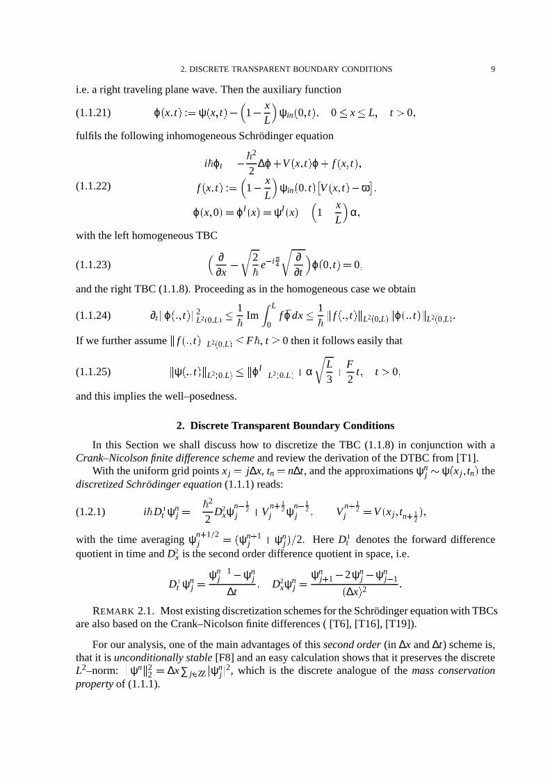
2. DiscreteTransparent Boundary Conditions
In this Sectionwe shall discusshow to discretizethe TBC (1.1.8) in conjunctionwith aCrank–Nicolsonfinitedifferenceschemeandreview thederivationof theDTBC from [T1].
With theuniformgrid pointsx j j∆x, tn n∆t, andtheapproximationsψnj + ψ
x j tn the
discretizedSchrodinger equation(1.1.1)reads:
i Dt ψnj 2
2D2
xψn 12
j Vn 1
2j ψn 1
2j V
n 12
j Vx j tn 1
2(1.2.1)
with the time averagingψn 1$ 2j
ψn 1j ψn
j % 2. Here Dt denotesthe forward differencequotientin timeandD2
x is thesecondorderdifferencequotientin space,i.e.
Dt ψnj ψn 1
j ψn
j
∆t D2
xψnj ψn
j 1 2ψn
j ψnj 1
∆x 2
REMARK 2.1. Mostexistingdiscretizationschemesfor theSchrodingerequationwith TBCs
arealsobasedon theCrank–Nicolsonfinite differences( [T6], [T16], [T19]).
For our analysis,oneof themainadvantagesof this secondorder (in ∆x and∆t) schemeis,thatit is unconditionallystable[F8] andaneasycalculationshowsthatit preservesthediscreteL2–norm: " ψn " 2
2 ∆x∑ j , ZZ & ψnj & 2, which is the discreteanalogueof the massconservation
propertyof (1.1.1).

10 1. THE SCHRODINGER EQUATION
In ordertoderivethisdiscretemassconservationpropertywemultiply (1.2.1)with iψn 1$ 2j % :
ψn 12
j Dt ψnj i
2ψn 1
2j D2
xψn 12
j i
Vn 1
2j ψn 1
2j
2 (1.2.2)
Summingit up for j ZZ (i.e. in absenceof boundaryconditions)giveswith summationbyparts
∑j , ZZ
ψn 12
j Dt ψnj i
2 ∑j , ZZ
Dx ψn 12
j
2 i ∑j , ZZ
Vn 1
2j ψn 1
2j
2 (1.2.3)
Finally, takingtherealpartby usingthesimpleidentity (“discreteproductrule”)
Dt ψn υn ψn 1
2Dt υn υn 1
2Dt ψn (1.2.4)
i.e. with υn ψn
Dt & ψn & 2 2Re- ψn 12Dt ψn . (1.2.5)
yieldstheconservationof themass:
Dt ∑j , ZZ
ψnj
2 0
(1.2.6)
REMARK 2.2. We remarkthatan arbitraryhigh (even)order conservativeschemefor theSchrodingerequation(1.1.1) can be obtainedby using the diagonalPade approximationstotheexponential[F1]. TheCrank–Nicolsonschemecorrespondsto secondorder, andthefourthorderis known in theODEliteratureasHammerandHollingsworthmethod[F2].
2.1. Discretization strategiesfor the TBC. We shallnow comparefour strategiesto dis-cretizethe TBC (1.1.8)with its mildly singularconvolution kernel. First we review a knowndiscretizationfrom the literature,wherethe analytic TBC in the equivalent form (1.1.10)atL J∆x wasdiscretizedin anad–hocfashion.
DiscretizedTBC of Mayfield. In [T16] Mayfield proposedtheapproximation
tn
0
ψxL tn τ e i VL τ!
τdτ / 1
∆x
n 1
∑m) 0
ψn m
J ψn m
J 1 e i VL m∆ttm 1
tm
dτ!τ
2!
∆t∆x
n 1
∑m) 0
ψn m
J ψn m
J 1 e i VL m∆t!m 1 !
m
(1.2.7)
wheresheusedtheleft–pointrectangularquadraturerule. Thisleadsto thefollowingdiscretizedTBC for theSchrodingerequation:
ψnJ ψn
J 1 ∆x
2B!
∆tψn
J n 1
∑m) 1
ψn mJ
ψn mJ 1
˜0 m(1.2.8)
with
B 2π
ei π4 ˜0 m e i VL m∆t!
m 1 !m
On thefully discretelevel this BC is no longerperfectlytransparent.For theresultingschemewith a homogeneousDirichlet BC at j 0 and(1.2.8),Mayfield obtainedthefollowing result:
2. DISCRETETRANSPARENT BOUNDARY CONDITIONS 11
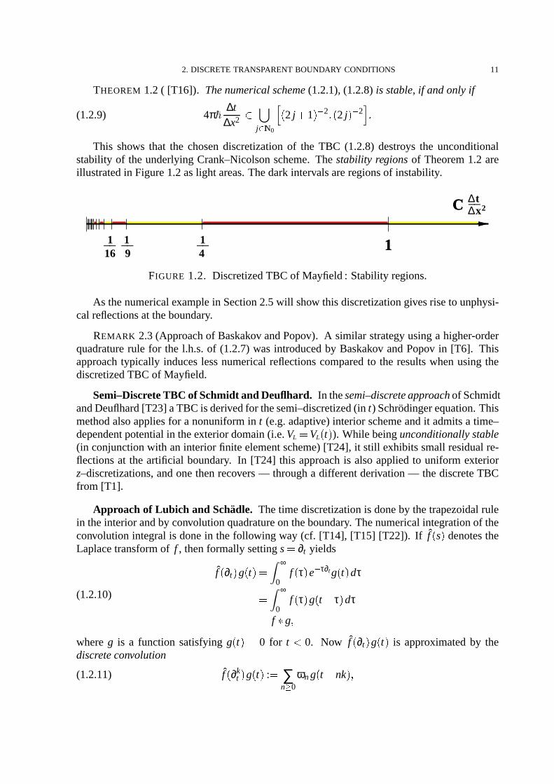
THEOREM 1.2( [T16]). Thenumericalscheme(1.2.1), (1.2.8)is stable, if andonly if
4π∆t
∆x2 j , IN0
2 j 1 2 2 j 2
(1.2.9)
This shows that the chosendiscretizationof the TBC (1.2.8) destroys the unconditionalstability of theunderlyingCrank–Nicolsonscheme.Thestability regionsof Theorem1.2 areillustratedin Figure1.2aslight areas.Thedarkintervalsareregionsof instability.
1111
∆x2__C ∆t
______4916
FIGURE 1.2. DiscretizedTBC of Mayfield: Stability regions.
As thenumericalexamplein Section2.5will show this discretizationgivesriseto unphysi-cal reflectionsat theboundary.
REMARK 2.3(Approachof Baskakov andPopov). A similar strategy usinga higher-orderquadraturerule for the l.h.s.of (1.2.7)wasintroducedby Baskakov andPopov in [T6]. Thisapproachtypically induceslessnumericalreflectionscomparedto the resultswhenusingthediscretizedTBC of Mayfield.
Semi–DiscreteTBC of SchmidtandDeuflhard. In thesemi–discreteapproachof SchmidtandDeuflhard[T23] aTBC is derivedfor thesemi–discretized(in t) Schrodingerequation.Thismethodalsoappliesfor a nonuniformin t (e.g.adaptive) interior schemeandit admitsa time–dependentpotentialin theexteriordomain(i.e.VL VL
t ). While beingunconditionallystable
(in conjunctionwith aninterior finite elementscheme)[T24], it still exhibits smallresidualre-flectionsat the artificial boundary. In [T24] this approachis alsoappliedto uniform exteriorz–discretizations,andonethenrecovers— througha differentderivation— thediscreteTBCfrom [T1].
Approachof Lubich and Schadle. Thetime discretizationis doneby thetrapezoidalrulein theinteriorandby convolutionquadratureon theboundary. Thenumericalintegrationof theconvolution integral is donein thefollowing way (cf. [T14], [T15] [T22]). If f
s denotesthe
Laplacetransformof f , thenformally settings ∂t yields
f∂t g
t ∞
0fτ e τ∂tg
t dτ
∞
0fτ g
t τ dτ
f 1 g(1.2.10)
whereg is a function satisfyinggt 0 for t 0. Now f
∂t g
t is approximatedby the
discreteconvolution
f∂k
t gt : ∑
n2 0ωng
t nk(1.2.11)

12 1. THE SCHRODINGER EQUATION
with the stepsize k ∆t. The quadratureweightsωn are definedas the coefficients of thegeneratingpowerseries:
∑n2 0
ωn ξn : fδξ k
& ξ & small
(1.2.12)
Hereδξ is thequotientof thegeneratingpolynomialsof alinearmultistepmethod,e.g.δ
ξ
1 ξ for theimplicit Eulermethodandδξ 2
1 ξ %
1 ξ for thetrapezoidalrule. If onechoosesfor thequadraturethesamenumericalschemeasin theinterior thenoneobtainsalsoareflection–freediscreteTBC.
DiscreteTBC. Insteadof usingan ad–hocdiscretizationof the analyticTBC like (1.2.7)we will constructdiscreteTBCsof the fully discretizedwhole–spaceproblem.Our new strat-egy solvesbothproblemsof thediscretizedTBCatnoadditionalcomputationalcosts.With ourDTBC thenumericalsolutiononthecomputationaldomain0 j J exactlyequalsthediscretewhole–spacesolution(on j ZZ) restrictedto thecomputationaldomain.Therefore,ouroverallschemepreventsany numericalreflectionsattheboundaryandinheritstheunconditionalstabil-ity of thewhole–spaceCrank–Nicolsonscheme(seeTheorem1.7).Thesedifferentapproaches,discretizationof theanalyticTBC and(semi–)discreteTBC, aresketchedin Figure1.3.
Discrete Schrodinger Equation..
same computational effort
(Analytic) Transparent BC
Discrete TBCDiscretized TBCArnold & Ehrhardt
semi-discrete TBCMayfield
Baskakov & Popov
only conditionally stable
numerical reflections
unconditionally stable
small reflections
Lubich & Schadle
unconditionally stable
reflection-free
Schmidt & Deuflhard..
..Schrodinger Equation
FIGURE 1.3. Discretizationstrategiesfor theTBC
Consequently, whenconsideringthediscretizationof TBCs,it shouldbeastandardstrategyto derivethediscreteTBCsof thefully discretizedproblem,ratherthenattemptingto discretizethe differentialTBC whenever it is possible. A comparisonof thesetwo strategiesfor a 1Dwavepropagationproblemis givenin [T10].
2.2. Derivation of the DTBC. To derivethediscreteTBC wewill now mimick thederiva-tion of theanalyticTBC from Section1 onadiscretelevel. TheCrank–Nicolsonscheme(1.2.1)canbewritten in theform:
iRψn 1
j ψn
j ∆2xψn 1
j ∆2xψn
j wVn 1
2j
ψn 1
j ψnj (1.2.13)

2. DISCRETETRANSPARENT BOUNDARY CONDITIONS 13
with
R 4∆x 2
∆t w 2
∆x 2
2 Vn 1
2j V
x j tn 1
2
where∆2xψn
j ψnj 1
2ψnj ψn
j 1, andR is proportionalto theparabolicmeshratio.Again,wewill only considertheright BC. In analogyto thecontinuousproblemweassume
for thepotentialandinitial data:Vnj VL const, j J 1, ψ0
j 0, j J 2 andsolve thediscreteright exteriorproblemby usingthediscreteanalogueof theLaplacetransformation,the
–transform:
- ψnj. ψ j
z : ∞
∑n) 0
ψnj z n z IC & z&3 1(1.2.14)
which is describedin moredetail in theAppendix.Hence,the
–transformedCrank–Nicolsonfinite differencescheme(1.2.13)for j J 1 reads
z 1 ∆2xψ j
z iR z 1 iκ
z 1 ψ j
z κ ∆t
2VL
(1.2.15)
Thetwo linearly independentsolutionsof theresultingsecondorder differenceequation
ψ j 1z 2 1 iR
2z 1z 1 iκ ψ j
z ψ j 1
z 0 j J 1(1.2.16)
take theform ψ jz ν j
1 2 z , j J 1, whereν1 2 z solve
ν2 2 1 iR2
z 1z 1 iκ ν 1 0
(1.2.17)
For thedecreasingmode(as j ∞) wehaveto require & ν1
z(&4 1andobtain(usingν1
z ν2
z
1) the
–transformedright DTBCas
ψJ 1z ν2
z ψJ
z (1.2.18)
Analogously, the
–transformedleft DTBC reads:
ψ1z ν2
z ψ0
z(1.2.19)
whereν2
z with & ν2
z#&5 1 is obtainedfrom asolutionto theleft discreteproblem, i.e. (1.2.16)
on therangej 1.
REMARK 2.4(DiscreteFactorization). If Sdenotestheusualshiftoperator givenby Sψ j
z
ψ j 1
z , thenanalogouslyto thecontinuouscase(cf. Remark1.3)thediscretizedSchrodinger
equation(1.2.16)canformally befactorizedas:
S ν1
z S ν2
z ψ j 1
z 0 j J 1(1.2.20)
which leadsto thesameDTBCs(1.2.18), (1.2.19).
It remainsto inversetransform(1.2.18)usingtheinversionrulesof the
–transformgivenin theAppendix.By thefollowing tediouscalculationthis canbeachievedexplicitly.
CALCULATION (of 1 - ν2
z . ). First we rewrite ν1 2 z as:
ν1 2 z 1 iR2
z 1z 1 iκ 6 iR
2z 1z 1 iκ 2 iR
2z 1z 1 iκ
1 iR2 Rκ
2 iR
zz 1 7
iR2
1z 1 Az2 2Bz C
(1.2.21)

14 1. THE SCHRODINGER EQUATION
with theconstants
A 1 iκ 1 iκ i
4R
(1.2.22a)
B 1 κ2 4κR
(1.2.22b)
C 1 iκ 1 iκ i
4R
(1.2.22c)
For theinverse
–transformweuse
Az2 2Bz C 1
! A
Az2 2Bz Cz
8 A 8 Cz
ACz2 2B
Cz 1
(1.2.23)
With theabbreviations
Fz µ z
z2 2µz 1 λ ! A
! C µ B
! A ! C(1.2.24)
we obtainfrom equation(1.2.23)
1z 1 Az2 2Bz C 1
! A
Az2 2Bz Czz 1 F
λz µ
1
! AA C
z E
z 1F
λz µ
! C λ λ 11z E
! A ! C
1z 1
Fλz µ
(1.2.25)
with E A 2B C. Theinversionrulesnow yield
1 ! Az2 2Bz Cz 1 ! C λδ0
n λ 1δ1n E
! A ! C
1 n δ0n 1 Pn
µ
! C λPnµ λ 1Pn 1
µ E
! A ! C
n 1
∑k) 0
1 n kPkµ
where 1 denotesthediscreteconvolution. Finally, weobtain
1 - ν1 2 z . 1 iR2 Rκ
2δ0
n iR 1 n
7iR ! C
2λ n λPn
µ Pn 1
µ E
! A ! C
n 1
∑k) 0
λ n kPkµ (1.2.26)
SinceC A wehave & λ & 1 with
λ A
! A ! C R 4κ Rκ2 2i
Rκ 2
1 κ2 R2 Rκ 4 2
(1.2.27)
Thereforewewrite
λ eiϕ with ϕ arctan2Rκ 2
R 4κ Rκ2
(1.2.28)
2. DISCRETETRANSPARENT BOUNDARY CONDITIONS 15
Weobtainfor theparameterµ:
µ R1 κ2 4κ
1 κ2 R2 Rκ 4 2
IR(1.2.29)
andit caneasilybeseenthat 1 µ 1 is valid. TheconstantE simply equals4 andwe get
τ E
! A ! C 4R
1 κ2 R2 Rκ 4 2
IR
(1.2.30)
Thechoiceof thesignin (1.2.26)canbejustifiedanalyticallyor simplyby testingit numer-ically. We finally obtaintheconvolutioncoefficients
0 n 1 - ν2
z . as
0 n 1 iR2 σ
2δ0
n iR
1 n i2
4 R2 σ2 R2
σ 4 2 e iϕ $ 2 99 e inϕ λPn
µ Pn 1
µ τ
n 1
∑k) 0
λ n kPkµ (1.2.31)
with σ Rκ andPn denotestheLegendrepolynomials.TheresultingdiscreteTBCsat thegridpointsx j j 0 J read
ψn1 0 0
0 ψn0 n 1
∑k) 1
0 n k0 ψk
0 n 1(1.2.32a)
ψnJ 1
0 0J ψn
J n 1
∑k) 1
0 n kJ ψk
J n 1
(1.2.32b)
Thesubscriptj of thecoefficients0 n indicatesat which boundarythevaluesareto be taken.
In thesequelmany parameterswill besuppliedwith this subscript.
2.3. The Asymptotic Behaviour of the Convolution Coefficients. We studytheasymp-
totic behaviour of the0 n
0 ,0 n
J in (1.2.32).It will turnout thatit is advantageousto reformulatetheDTBC usingnew coefficients.Afterwardsweshallderivearecursionformulafor thesenewcoefficientsandcomparetheir decayratewith thedecayrateof thecontinuousintegral kernelin (1.1.8),(1.1.9).
The summedconvolution coeffcients. Firstwewantto studytheasymptoticbehaviourof
theconvolutioncoefficients0 n
j , j 0 J. With thenotationµj cosθ j , 0 θ j π, weusethefollowing classicalresulton theasymptoticpropertyof theLegendrepolynomials:
LEMMA 1.3(Theorem8.21.2(Formulaof Laplace),[S7]).
Pncosθ j
!2!
π sinθ j
cosn 1
2 θ j π
4!n O
n 3$ 2 0 θ j π
(1.2.33)
Theboundfor theerror termholdsuniformlyin theinterval ε θ j π ε.
From this lemmawe concludethat limn: ∞ Pnµj 0 holds. Consequently, the coefficients
have thefollowing asymptoticbehaviour for n ∞:
0 nj
iR 1 n + iτ j
24
R2 σ2
j R2 σ j 4 2 e iϕ j $ 2 1 n
n 1
∑k) 0
e iϕ j kPkµj (1.2.34)

16 1. THE SCHRODINGER EQUATION
Using
limn: ∞
n 1
∑k) 0
e iϕ j kPkµj 1
1 2µj λ j λ j2
1
2λ j
1
Reλ j µj
12R
4R2 σ2
j R2 σ j 4 2 eiϕ j $ 2
(1.2.35)
we finally obtain
0 nj + iR
1 n iτ j
4R
R2 σ2
j R2 σ j 4 2
1 n 2iR 1 n (1.2.36)
Thesequence0 n
j is asymptoticallyanalternating,purelyimaginarysequence,whichmaylead(on thenumericallevel) to subtractivecancellationin (1.2.32). To circumventthis problemweconsiderthesummedcoefficients
s nj : 0 n
j 0 n 1j n 1 s
0j : 0 0
j j 0 J (1.2.37)
andcompute:
0 0j 1 i
R2 σ j
2 i
24
R2 σ2
j R2 σ j 4 2 eiϕ j $ 2
1 iR2 σ j
2 i
2 R2 4σ j σ2
j 2iRσ j 2(1.2.38)
0 1j iR i
24
R2 σ2
j R2 σ j 4 2 e iϕ j $ 2 µj e iϕ j τ j (1.2.39)
andfor n 2 wecomputeusingthedefinitionof E:
s nj i
24
R2 σ2
j R2 σ j 4 2 eiϕ j $ 2e inϕ j
Pnµj λ j λ 1
j τ j
) 2µj
Pn 1µj Pn 2
µj (1.2.40)
With therecurrencerelationof theLegendrepolynomials
µjPn 1µj n
2n 1Pn
µj n 1
2n 1Pn 2
µj n 1
we finally get
s nj i
24
R2 σ2
j R2 σ j 4 2 eiϕ j $ 2e inϕ j
Pnµj Pn 2
µj
2n 1 n 2
(1.2.41)
REMARK 2.5. Thecoefficient0 0
j canalsobecalculatedwith [S3,Theorem39.1]by
0 0j lim
z: ∞ν2
z 1 i
R2 σ j
2 i
2 R iσ j R i
σ j 4 (1.2.42)
Wesummarizeour resultsin thefollowing theorem:
2. DISCRETETRANSPARENT BOUNDARY CONDITIONS 17
THEOREM 1.4( [T1]). Theleft (at j 0) andright (at j J) discreteTBCsfor theCrank–Nicolsondiscretization(1.2.1)of the1D Schrodinger equationare respectively
ψn1 s
00 ψn
0 n 1
∑k) 1
s n k0 ψk
0 ψn 1
1 n 1(1.2.43a)
ψnJ 1
s 0J ψn
J n 1
∑k) 1
s n kJ ψk
J ψn 1
J 1 n 1(1.2.43b)
with
s nj 1 i
R2 σ j
2δ0
n 1 iR2 σ j
2δ1
n α j e inϕ jPn
µj Pn 2
µj
2n 1(1.2.44)
ϕ j arctan2R
σ j 2
R2 4σ j σ2
j
µj R2 4σ j σ2j
R2 σ2j R2
σ j 4 2
σ j 2∆x2
2 Vj α j i2
4R2 σ2
j R2 σ j 4 2 eiϕ j $ 2 j 0 J
Pn denotestheLegendrepolynomials(P 1 ; P 2 ; 0) andδ jn theKronecker symbol.
ThePn only have to beevaluatedat the two valuesµ0 µJ 1 1 , andhencethenumeri-cally stablerecursionformulafor theLegendrepolynomialscanbeused[E2].
The recurrenceformula for the summedcoefficients. In this subsectionwe shall give
two different derivationsfor the recursionformula of the convolution coefficients s nj . The
first oneis basedon the explicit representation(1.2.41)of s nj by first calculatinga recursion
formulafor Pn 1µj Pn 1
µj . Thesecondderivationdoesnotrequiretheexplicit form of the
coefficientss nj but only thegrowthfunctionsν1 2 z from the
–transformedDTBCs(1.2.18)
and(1.2.19).
FIRST DERIVATION: Herewe startwith the standard recursion formula [S1] for the Le-gendrepolynomialsPn 1
µj , Pn 1
µj :
n 1 Pn 1µj
2n 1 µjPnµj nPn 1
µj n 0
n 1 Pn 1µj
2n 3 µjPn 2µj
n 2 Pn 3µj n 2(1.2.45)
and
Pn 1µj 2µjPn 2
µj Pn 3
µj Pn 3
µj Pn 1
µj
2n 3 n 2
(1.2.46)
TheexpressionPn 1µj Pn 1
µj is convertedin thefollowing way:
n 1 Pn 1
µj Pn 1
µj
2n 1 µjPn
µj
2n 1 2n 3n 1
µjPn 2µj
2n 1 n 2n 1
Pn 3µj
2n 1 µj Pn
µj Pn 2
µj
n 2 2n 12n 3
Pn 1µj Pn 3
µj

18 1. THE SCHRODINGER EQUATION
wherewehaveusedtherelation
Pn 3µj µjPn 2
µj 1
2Pn 3
µj Pn 1
µj
2n 3 Pn 1
µj Pn 3
µj
n 12n 3
Pn 1µj Pn 3
µj
Finally, weobtainfor n 2 thefollowing recursionformulafor Pn 1µj Pn 1
µj :
(1.2.47) Pn 1µj Pn 1
µj
2n 1n 1
µj Pnµj Pn 2
µj
n 2 2n 1n 1 2n 3 Pn 1
µj Pn 3
µj
Sincethes nj aredeterminedby
s nj α j
λ nj
2n 1Pn
µj Pn 2
µj n 2(1.2.48)
we getfrom (1.2.47)therecurrencerelation for thesummedconvolutioncoefficients:
s n 1j 2n 1
n 1µjλ 1
j s nj
n 2n 1
λ 2j s
n 1j n 2(1.2.49)
which canbeusedaftercalculatingthefirst valuess nj for n 0 1 2 by theformula(1.2.44).
SECOND DERIVATION: Next weshallpresentanalternativederivationof thefirst convolu-
tion coefficientss nj , n 0 1 2 andtherecurrencerelation(1.2.49). Theadvantageof thisalter-
nativeapproachis thatweshallonly needthegrowthfunctionsν1 2 z from the
–transformedDTBCs(1.2.18)and(1.2.19). Hencethis approachmight alsoapplyto a biggerclassof linearevolutionequations,whereit is notpossible(or too tedious)to deriveanexplicit representationof theconvolutioncoefficients.
We remarkthat an even moreadvantageousapproachmight be basedon the polynomialequation(1.2.17)for thegrowth functionν
z , ratherthanon its explicit solution. Thebenefit
of sucha strategy would lie in the possibility to obtain the convolution coefficients also forhigherorderdifferenceschemes,thatwould leadto quartic(or evenhigherorder)equationsforνz . To our knowledgethis has,however, notbeenaccomplishedyet.
In this secondapproachweshallfirst deriveafirst orderODEfor thegrowth functionνz ,
which is explicitly givenby (1.2.21). In fact,it is moreconvenientto consider
νz :
z 1 ν z ∞
∑n) 1
s n 1j z n (1.2.50)
Usingtheconstants(1.2.22)and(1.2.24)it hastheexplicit form
ν1 2 z z 1 iR2 σ j
2 1 iR2 σ j
26 i
2 R2 4σ j σ2j z2λ
µ 2z 1
λµ
(1.2.51)
Theindex j 0 J againdenotesthegrid pointwheretheDTBC is to beconstructed.Multiply-
ing ν< dνdz
by z2λµ
2z 1λµ
thenyieldsaninhomogeneousfirst orderODE for νz :
z2λµ
2z 1λµ
ν< z zλµ
1 νz β
z : β 1 z β 0 (1.2.52)

2. DISCRETETRANSPARENT BOUNDARY CONDITIONS 19
with
β 1 λµ
1 iR2 σ j
2 1 iR2
σ j
2
β 0 1λµ
1 iR2 σ j
2 1 iR2 σ j
2
(1.2.53)
Its generalsolutionincludesν1 2 z asdefinedin (1.2.51).UsingtheLaurentseries(1.2.50)of
ν andν< in (1.2.52)immediatelyyieldsthedesiredrecursionfor thecoefficientss nj :
λµ
s 1j
s 0j β 1
2λµ
s 2j s
1j 1
λµs 0j β 0
n 1 s n 1
j 2n 1 µ
λs nj
n 2 1
λ2s n 1j 0 n 2
(1.2.54)
whichcoincideswith (1.2.49).Thestartingcoefficientof therecursioncanbedeterminedasin (1.2.42):
s 0j lim
z: ∞
νzz 1 i
R2 σ j
26 i
2R2 4σ j σ2
j λµ
Here,thesignhasto befixedsuchthat & ν1
z(&= 1 for the right DTBC and & ν2
z(&= 1 for the
left DTBC. Thiscanbedonefor e.g.for z ∞.
STABILITY OF THE RECURRENCE RELATION: For proving that the recurrencerelation(1.2.49)is well–conditionedwe follow the notationin [E2] andwrite (1.2.49)as the secondorderdifferenceequation
s n 1j a
nj s
nj b
nj s
n 1j 0 n 2(1.2.55)
with
a nj 2n 1
n 1µjλ 1
j b nj n 2
n 1λ 2
j > 0
(1.2.56)
Therearetwo linearly independentsolutionss nj 1, s
nj 2 to (1.2.55).If they have theproperty
limn: ∞
s nj 2
s nj 1 0(1.2.57)
thens nj 2 is calleda minimalsolutionandseriousnumericalproblemsariseif onetriesto com-
putethe solutions nj 2 in a straightforward way by usingthe recursion(1.2.49). If thereis an
errorin theinitial databut recurringwith infinite precisionthentherelativeerrorof theintended
approximationto s nj 2 becomesarbitrarily large. Methodsof calculatingminimal solutionsof
three–termrecurrencerelationscanbefoundin [E2]. To provethat(1.2.49)is well–conditionedwehave to show thattheseekedsolutionis not a minimal solutionto (1.2.55). This typeof so-lution is calleddominant.

20 1. THE SCHRODINGER EQUATION
Sincethecoefficientsa nj , b
nj in (1.2.55)have thefinite limits
a j limn: ∞
a nj 2µjλ 1
j 2B j
A j b j lim
n: ∞b nj λ 2
j Cj
A j j 0 J (1.2.58)
onecalls(1.2.55)aPoincaredifferenceequationand
Φ jt t2 a j t b j(1.2.59)
thecharacteristicpolynomialof (1.2.55).Thecharacteristicpolynomialhasthecomplex conju-
gatezerost 1 2j
B j 6 i 4% R% A j . Thezeroshave thesamemoduli: & t 1 2j & 1, andthereforethe classicalTheorem of Poincare (formulatedbelow for the specialcaseof a second–orderdifferenceequation)cannotbe appliedto distinguishtwo solutionswith distinct asymptoticproperties.
THEOREM 1.5(Poincare Theorem,[E1]). Supposethat thezerost 1j , t
2j of thecharacter-
istic polynomial(1.2.59)havedistinctmoduli.Thenfor anynontrivial solutions nj of (1.2.55)
limn: ∞
s n 1j
s nj
t kj
for k 1 or k 2.
REMARK 2.6. If equation(1.2.55)hascharacteristicrootswith equalmodulithenPoincare’sTheoremmayfail (cf. exampleof Perron[E1]).
It is well–known that the LegendrepolynomialsPnµj andthe Legendre functionsof the
secondkind (of order zero) Qnµj satisfy the samethree–termrecurrencerelation (1.2.45).
Therefore,the two linearly independentsolutionsto (1.2.55)are the convolution coefficients
s nj 1 s
nj (1.2.48)ands
nj 2 givenby
s nj 2 β j
λ nj
2n 1Qn
µj Qn 2
µj n 2(1.2.60)
with someconstantβ j .Now we want to studytheasymptoticbehaviourof thesetwo solutions.With thenotation
µj cosθ j , 0 θ j π, weuseLemma1.3whichgives
Pncosθ j Pn 2
cosθ j 2
!2 sinθ j!
πsin
n 1
2 θ j π
4!n O
n 3$ 2 (1.2.61)
andfrom (1.2.48)weseethat
s nj + α j
!2 sinθ j!
πλ n
j
sinn 1
2 θ j π
4n 1
2 ! n n ∞
(1.2.62)
An analogousformulato (1.2.33)for theLegendrefunctionsof thesecondkind Qnµj is given
by thefollowing lemma:
LEMMA 1.6(Theorem8.21.14,[S7]). For 0 θ j π
Qncosθ j
!π!
2 sinθ j
cosn 1
2 θ j π4!
n On 3$ 2 (1.2.63)

2. DISCRETETRANSPARENT BOUNDARY CONDITIONS 21
Thisholdsuniformlyin theinterval ε π ε .As beforewecandeducefrom (1.2.60)that
s nj 2 + β j
!π sinθ j!
2λ n
j
sinn 1
2 θ j π4
n 12 ! n
n ∞(1.2.64)
holds.Thereforetheratioof thetwo solutionsbehavesasymptoticallyas
s nj 2
s nj
+ β j
α j
π2
sinn 1
2 θ j π4
sinn 1
2 θ j π
4 β j
α j
π2
tann 1
2 θ j π
4 n ∞
i.e.neithers nj nors
nj 2 canbeaminimalsolution.Consequently, theproblemof determiningthe
requiredvaluesof theconvolutioncoefficientsis well–conditioned[E2]: they canbecomputednumericallyfrom therecurrencerelation(1.2.49)in astablefashion.
REMARK 2.7. In thespecialcaseθ j π % 2 weobserve theasymptoticbehaviour
s nj 2
s n 1j
+ β j
α j
π2
n ∞
Decayrate of the convolution kernel. Since & λ j & 1 therelation(1.2.62)shows thats n0 ,
s nJ O
n 3$ 2 , whichagreeswith thedecayof theconvolutionkernelin thedifferentialTBCs
(1.1.8), (1.1.9). To show this propertywe considerthe left TBC (1.1.9) andobtainafter anintegrationby parts
ψx0 t c
ddt
t
0
ψ0 τ !t τ
dτ
cddt
t
t ε
ψ0 τ !t τ
dτ 12
t ε
0
ψ0 τ
t τ 3$ 2 dτ ψ0 t ε !
ε
(1.2.65)
with
c 2π
e i π4 1 i!
π
(1.2.66)
To comparethediscreteconvolution in theDTBCswith thecontinuousconvolution in thedif-ferentialTBCsweconsiderthefollowing discretization(with ε ∆t)
c2
t ε
0
ψ0 τ
t τ 3$ 2 dτ / c2
n 1
∑k) 1
ψk0
n k ∆t 3$ 2∆t
(1.2.67)
If wecomparethis with (1.2.43a)written in theform
ψn1 ψn
0
∆x 1∆x
n 1
∑k) 1
s n k0 ψk
0 ψn 1
1 s 00 ψn
0 ψn
0 n 1(1.2.68)
wewould roughlyexpect
s n0 + c∆x
2!
∆tn 3$ 2 i 1
2!
π∆x!∆t
n 3$ 2 n ∞
(1.2.69)
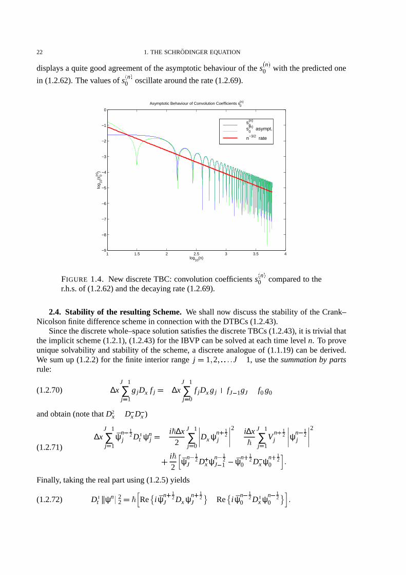
In Figure1.4 we comparethe s n0 for increasingtime levelsn with the r.h.s.of (1.2.62). The
usedparametersare 1, ∆t 10 6, ∆x 1% 160andthepotentialis setto zero. Figure1.4
22 1. THE SCHRODINGER EQUATION
displaysa quitegoodagreementof theasymptoticbehaviour of thes n0 with thepredictedone
in (1.2.62). Thevaluesof s n0 oscillatearoundtherate(1.2.69).
1 1.5 2 2.5 3 3.5 4−9
−8
−7
−6
−5
−4
−3
−2
−1
0
Asymptotic Behaviour of Convolution Coefficients s0(n)
log10
(n)
log 10
(s0(n
) )
s0(n)
s0(n) asympt.
n−3/2 rate
FIGURE 1.4. New discreteTBC: convolution coefficientss n0 comparedto the
r.h.s.of (1.2.62)andthedecayingrate(1.2.69).
2.4. Stability of the resulting Scheme.We shall now discussthestability of theCrank–Nicolsonfinite differenceschemein connectionwith theDTBCs(1.2.43).
Sincethediscretewhole–spacesolutionsatisfiesthediscreteTBCs(1.2.43), it is trivial thattheimplicit scheme(1.2.1),(1.2.43)for theIBVP canbesolvedat eachtime level n. To proveuniquesolvability andstability of thescheme,a discreteanalogueof (1.1.19)canbe derived.We sumup (1.2.2)for thefinite interior range j 1 2 ? J 1, usethesummationby partsrule:
∆xJ 1
∑j ) 1
g jD @x f j ∆xJ 1
∑j ) 0
f jDxg j fJ 1gJ f0 g0(1.2.70)
andobtain(notethatD2x D @x Dx )
∆xJ 1
∑j ) 1
ψn 12
j Dt ψnj i ∆x
2
J 1
∑j ) 0
Dx ψn 12
j
2 i∆x J 1
∑j ) 1
Vn 1
2j ψn 1
2j
2
i2
ψn 12
J Dx ψn 12
J 1 ψn 1
20 Dx ψn 1
20
(1.2.71)
Finally, takingtherealpartusing(1.2.5)yields
Dt " ψn " 22 Re i ψn 1
2J D @x ψn 1
2J
Re i ψn 12
0 Dx ψn 12
0 (1.2.72)

2. DISCRETETRANSPARENT BOUNDARY CONDITIONS 23
with thediscreteL2–normdefinedby " ψn " 22 : ∆x∑J 1
j ) 1 & ψnj & 2. After summationwith respectto
thetime index wegetfrom (1.2.72):
" ψN 1 " 22 " ψ0 " 2
2 ∆t Re iN
∑n) 0
ψn 12
J D @x ψn 12
J Re i
N
∑n) 0
ψn 12
0 Dx ψn 12
0
" ψ0 " 22 ∆t
∆xRe i
N
∑n) 0
ψn 12
J
ψn 1
2J 1 ˜0 n
J ∆t∆x
Re iN
∑n) 0
ψn 12
0
ψn 1
20 1 ˜0 n
0
(1.2.73)
where ˜0 nj : 0 n
j δ0
n, j 0 J. Again, asin thecontinuouscase,it remainsto show that theboundary–memory–termsin (1.2.73)areof positivetype. Weconcentrateon theboundarytermat j J anddefinethefinite sequences
fn ψn 12
J 1 ˜0 nJ gn ψn 1
2J n 0 1 N (1.2.74)
with fn gn 0 for n N, i.e.Re- i ∑Nn) 0 fn gn
. 0 is to show. A
–transformationusingthetransformedDTBC (1.2.18)yields
- fn. f
z z 1
2ψN
Jz ν2
z 1
iR4
ψNJz z 1 iκ
z 1 7 Az2 2Bz C (1.2.75)
whereψNJ
z ∑N
n) 0 ψnJz n is analyticon & z&A 0. Theexpressionabove in thecurly bracketsis
analyticfor & z&= 1 andcontinuousfor & z&B 1, sincethezerosz1 2 of thesquareroot aregivenby z1 2
B 6 i 4% R% A with & z1 2 & 1. Thereforefz is analyticon 1 *& z&3 ∞. Notethatwe
have to choosethesignin (1.2.75)suchthatit matcheswith ν2
z for & z& sufficiently large. For
thesecondsequencegn weobtain
- gn. g
z z 1
2ψN
Jz(1.2.76)
i.e. gz is analyticon0 *& z&3 ∞.
Now thebasicideais to usePlancherel’s theoremin theform (Z.7) whichgives
Re iN
∑n) 0
fn gn 18π
Re i2π
0& z 1 & 2 ψN
Jz 2 ν2
z 1
z) eiϕdϕ
18π
Im2π
0ν2
eiϕ dϕ
(1.2.77)
Weremarkthatthepoleof ν2
z atz 1 is “cancelled”by & z 1 & 2. From(1.2.77)weconclude
thatthediscreteL2–norm(1.2.73)is non–increasingin time if
Im ν2
eiϕ C 0 D ϕ E 0 2π F(1.2.78)
holds.Thispropertyof ν2 canbeshown in thefollowing way. If wedefine
y iR2
z 1z 1 iκ(1.2.79)
then(1.2.21)simply reads
ν2
y 1 y y
2 y (1.2.80)
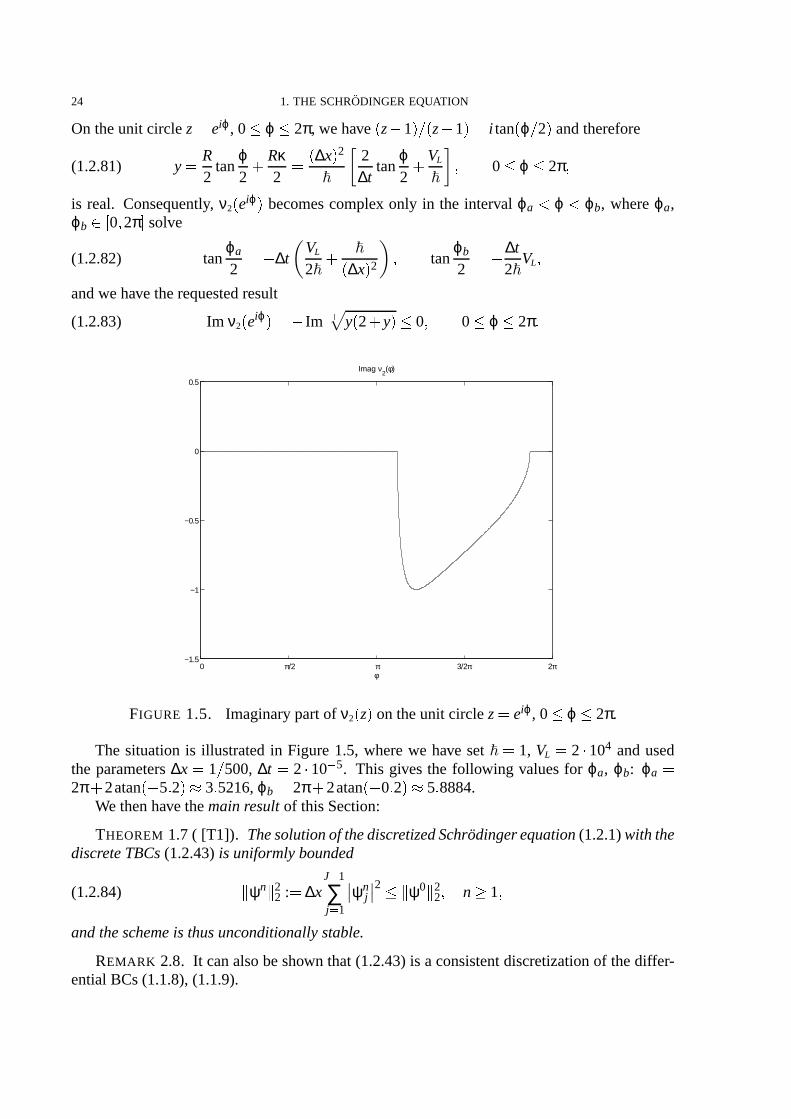
24 1. THE SCHRODINGER EQUATION
On theunit circlez eiϕ, 0 ϕ 2π, wehavez 1%
z 1 i tanϕ % 2 andtherefore
y R2
tanϕ2 Rκ
2 ∆x 2 2
∆ttan
ϕ2 VL 0 ϕ 2π (1.2.81)
is real. Consequently, ν2
eiϕ becomescomplex only in the interval ϕa ϕ ϕb, whereϕa,
ϕb G 0 2π solve
tanϕa
2 ∆tVL
2 ∆x 2 tan
ϕb
2 ∆t2
VL (1.2.82)
andwehave therequestedresult
Im ν2
eiϕ Im y
2 yH 0 0 ϕ 2π
(1.2.83)
0 π/2 π 3/2π 2π −1.5
−1
−0.5
0
0.5
φ
Imag ν2(φ)
FIGURE 1.5. Imaginarypartof ν2
z on theunit circlez eiϕ, 0 ϕ 2π.
The situationis illustratedin Figure1.5, wherewe have set 1, VL 2 9 104 andusedthe parameters∆x 1% 500, ∆t 2 9 10 5. This givesthe following valuesfor ϕa, ϕb: ϕa 2π 2atan
52/ 3
5216,ϕb 2π 2atan
02/ 5
8884.
We thenhave themainresultof this Section:
THEOREM 1.7( [T1]). Thesolutionof thediscretizedSchrodingerequation(1.2.1)with thediscreteTBCs(1.2.43)is uniformlybounded
" ψn " 22 : ∆x
J 1
∑j ) 1
ψnj
2 I" ψ0 " 22 n 1(1.2.84)
andtheschemeis thusunconditionallystable.
REMARK 2.8. It canalsobeshown that(1.2.43)is a consistentdiscretizationof thediffer-entialBCs(1.1.8),(1.1.9).

2. DISCRETETRANSPARENT BOUNDARY CONDITIONS 25
Simplified DTBC. Thedecayof thes nj shown in (1.2.62)motivatesto considera simpli-
fiedversionof theDTBC (1.2.43)with theconvolution coefficientscut off at anindex M. Thismeansthatonly the“recentpast”(i.e.M time levels)is takeninto accountin theconvolution in(1.2.43):
ψn1 s
00 ψn
0 n 1
∑k) n M
s n k0 ψk
0 ψn 1
1 n 1(1.2.85a)
ψnJ 1
s 0J ψn
J n 1
∑k) n M
s n kJ ψk
J ψn 1
J 1 n 1
(1.2.85b)
This,of course,reducestheperfectaccuracy of theDTBC (1.2.43),but it is numericallycheaperwhile still yielding reasonableresultsfor moderatevaluesof M. We remarkthatthenumericalstability of the schemewith simplified DTBC dependingon the valueof M is not anymoreobtainedautomatically. This issueis currentlyunderinvestigation[D1].
2.5. Numerical Results. In this Sectionwe presentanexampleto comparethenumericalresultsfrom usingour new discreteTBC to thesolutionusingotherdiscretizationstrategiesoftheTBC for theSchrodingerequation(1.1.1). We alsoshow thenumericaleffect if theDTBCis simplified by (1.2.85). Due to its construction,our DTBC yields exactly (up to round–offerrors)thenumericalwhole–spacesolutionrestrictedto thecomputationalinterval 0 L . Thecalculationwith discretizedTBCs requiresthe samenumericaleffort. However, the solutionmay(on coarsegrids)stronglydeviatefrom thenumericalwhole–spacesolution.
Example. This exampleshows a simulationof a right travelling Gaussianbeam ψI x exp
i100x 30
x 0
5 2 at four consecutive time stepsevolving underthe freeSchrodinger
equation( 1)with therathercoarsespacediscretization∆x 1% 160andthetimestep∆t 2 910 5. DiscretizingtheanalyticTBCsvia (1.2.7)(schemeof Mayfield [T16]) or asin BaskakovandPopov [T6] inducesstrongnumericalreflections. Our discreteTBCs (1.2.43),however,yield thesmoothnumericalsolutionto thewhole–spaceproblem,restrictedto thecomputationalinterval 0 1 (up to round–off errors).
Weobservein Figure1.6theartificial reflectionstravelling to theleft inducedbydiscretizingtheanalyticTBC while thesolutionwith thenew discreteTBC leavethecomputationaldomainwithout any numericalreflections. At time t 0
01 the solutionwith the DTBC hasalmost
completelyleft the domain 0 1 andthe solutionswith discretizedTBCs containa reflectedwavepacket with themaximummodulus(whichcorrespondsto themaximumerror)of around0.17for theapproachof Mayfieldandaround0.025in caseof thediscretizedTBC of BaskakovandPopov.
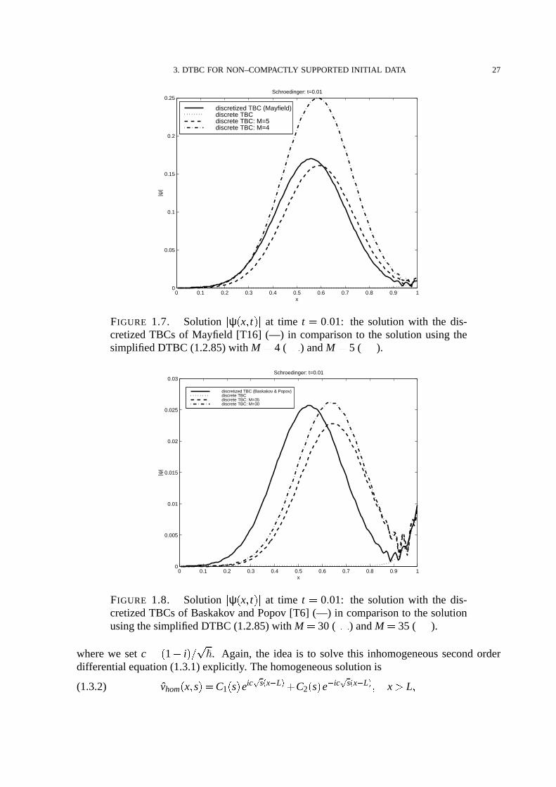
Now we presenttheresultswhenusingthesimplifiedDTBC (1.2.85)andwantto comparethe outcomewith the discretizedTBCs at time t 0
01. All theseboundaryconditionsneed
a comparablecomputationaleffort. Thecut–off valueM is chosenappropriately, suchthat thesimplified DTBC yields similar resultswith respectto the numericalreflectionsat the rightboundaryx 1. As a referencewealsoplot thesolutionwith thediscreteTBCs( 99?9 ).
Weseein Figure1.7thatthesolutionwith thesimplifieddiscreteTBCs(1.2.85)with M 5is alreadybetterthanthesolutionwith thediscretizedanalyticTBCs(1.2.7)from [T16].
We observe in Figure1.8 that the error of the solutionwith the discretizedanalyticTBCfrom [T6]. lies betweentheerrorsof thesolutionswith thesimplifieddiscreteTBCs (1.2.85)usingthecut–off valueM 30,M 35.

26 1. THE SCHRODINGER EQUATION
0 0.1 0.2 0.3 0.4 0.5 0.6 0.7 0.8 0.9 10
0.2
0.4
0.6
0.8
1
x
|ψ|
Schroedinger: t=0.004
new discrete TBCdiscretized TBC (Mayfield)discretized TBC (Baskakov & Popov)
0 0.1 0.2 0.3 0.4 0.5 0.6 0.7 0.8 0.9 10
0.1
0.2
0.3
0.4
0.5
0.6
0.7
0.8
0.9
1
x
|ψ|
Schroedinger: t=0.006
new discrete TBCdiscretized TBC (Mayfield)discretized TBC (Baskakov & Popov)
0 0.1 0.2 0.3 0.4 0.5 0.6 0.7 0.8 0.9 10
0.05
0.1
0.15
0.2
0.25
x
|ψ|
Schroedinger: t=0.008
new discrete TBCdiscretized TBC (Mayfield)discretized TBC (Baskakov & Popov)
0 0.1 0.2 0.3 0.4 0.5 0.6 0.7 0.8 0.9 10
0.02
0.04
0.06
0.08
0.1
0.12
0.14
0.16
0.18
x
|ψ|
Schroedinger: t=0.01
new discrete TBCdiscretized TBC (Mayfield)discretized TBC (Baskakov & Popov)
FIGURE 1.6. Solution & ψ x t (& at time t 0
004, t 0
006, t 0
008, t
001: the solutionwith the new discreteTBCs (—) coincideswith the whole–
spacesolution,while thesolutionwith thediscretizedanalyticTBCs(1.2.7)from[T16] ( @J@J@ ) or from [T6] ( 999 ) introducesstrongnumericalreflections.
3. DTBC for non–compactlysupported Initial Data
In this Sectionwe show how to dropassumption(A1), i.e. herethe initial dataψI x neednot becompactlysupportedinsidethecomputationaldomain.We only assumethat the initialfunctionψI x is continuous.Firstwereview thederivationof theTBC on thecontinuouslevelandmimick thisderivationstrategy afterwardsfor thediscretescheme.
3.1. The Transparent Boundary Condition. Herewe review thederivationof the (con-tinuous)TBC from [T13]. In the caseof the free Schrodingerequationwith non–compactlysupportedinitial dataψI the Laplacetransformed(using(L.2)) right exterior problem(1.1.5)now reads
vxx c2sv c2ψI x x L (1.3.1a)
vL s Φ
s(1.3.1b)
3. DTBC FOR NON–COMPACTLY SUPPORTED INITIAL DATA 27
0 0.1 0.2 0.3 0.4 0.5 0.6 0.7 0.8 0.9 10
0.05
0.1
0.15
0.2
0.25
x
|ψ|
Schroedinger: t=0.01
discretized TBC (Mayfield)discrete TBCdiscrete TBC: M=5discrete TBC: M=4
FIGURE 1.7. Solution & ψ x t #& at time t 0
01: the solution with the dis-
cretizedTBCs of Mayfield [T16] (—) in comparisonto the solutionusingthesimplifiedDTBC (1.2.85)with M 4 ( @JK @JK ) andM 5 ( @J@J@ ).
0 0.1 0.2 0.3 0.4 0.5 0.6 0.7 0.8 0.9 10
0.005
0.01
0.015
0.02
0.025
0.03
x
|ψ|
Schroedinger: t=0.01
discretized TBC (Baskakov & Popov)discrete TBCdiscrete TBC: M=35discrete TBC: M=30
FIGURE 1.8. Solution & ψ x t #& at time t 0
01: the solution with the dis-
cretizedTBCsof Baskakov andPopov [T6] (—) in comparisonto thesolutionusingthesimplifiedDTBC (1.2.85)with M 30 ( @JK @JK ) andM 35( @J@J@ ).
wherewe setc 1 i % ! . Again, the idea is to solve this inhomogeneoussecondorder
differentialequation(1.3.1)explicitly. Thehomogeneoussolutionis
vhomx s C1
s eic 8 s x L C2
s e ic 8 s x L x L (1.3.2)
28 1. THE SCHRODINGER EQUATION
andaccordingto [M3, (14.31)]aparticularsolutionof (1.3.1a)is givenby
vparx s c
2i!
s
x
Leic 8 s x xL ψI x< dx< x
Leic 8 s xL x ψI x< dx< x L (1.3.3)
i.e. thegeneralsolutionis
vx s vhom
x s vpar
x s
C1s e ic 8 sL c
2i!
s
x
Le ic 8 sxL ψI x< dx< eic 8 sx
C2s eic 8 sL c
2i!
s
∞
Leic 8 sxL ψI x< dx< c
2i!
s
∞
xeic 8 sxL ψI x< dx< e ic 8 sx
(1.3.4)
We notethatthelasttermin (1.3.4)is boundedfor fixeds andx ∞. Sincethesolutionshaveto decreaseasx ∞, the ideais to eliminatethegrowing factore ic 8 sx e
1 @ i 8 sx by simplychoosing
C2s c
2i!
s
∞
Leic 8 s xL L ψI x< dx< (1.3.5)
Consequently, weobtainC1s from theboundarycondition(1.3.1b):
C1s Φ
s c
2i!
s
∞
Leic 8 s xL L ψI x< dx< (1.3.6)
Fromthis wegetthefollowing representationof thetransformedright TBC:
vxL s ic
!sC1
s c2
2
∞
Leic 8 s xL L ψI x< dx<
ic!
sΦs c2
∞
Leic 8 s xL L ψI x< dx<
(1.3.7)
It remainsto inversetransform(1.3.7). If we furtherassumethat ψI is continuouslydifferen-tiable,thenintegrationby partsyields:
vxL s ic!
ssΦ
s ψI L ic!
s
∞
Leic 8 s xL L ψI
xx< dx< (1.3.8)
TheinverseLaplacetransformationusingtheconvolution theoremgives
ψxL t ic!
π
t
0
ψtL τ !
t τdτ ic M 1 1!
s
∞
Leic 8 s xL L ψI
xx< dx<
(1.3.9)
Finally, if ψIx is integrablefor x L, Levy proved( [T13, Theorem3.1]) thattheintegrationand
the inverseLaplacetransformcanbe interchangedin (1.3.9)to obtain(with (IL.8)) the rightTBC
ψxL t ic!
π
t
0
ψtL τ !
t τdτ ic!
πt
∞
LψI
xx e
i N x @ LO 22
t dx
(1.3.10)
REMARK 3.1. Clearly, if ψI x 0 for x L then(1.3.10)reducesto the previously ob-tainedright TBC (1.1.8)in thepotential–freecase(notethat !
2e i π4 i 1).
As motivatedin thepreviousSectionwewill not discretizethis TBC. Insteadwewill shownow how to derive theTBC on a fully discretelevel by mimicking thederivationof thecontin-uousTBC.
3. DTBC FOR NON–COMPACTLY SUPPORTED INITIAL DATA 29
3.2. The DiscreteTransparent Boundary Condition. First we show how to solve anin-homogeneoussecondorderdifferenceequationwith constantcoefficientsof theform
U j 1 aU j bU j 1 γ j j J 1
(1.3.11)
Wealreadyknow from Section2 thatthetwo linearly independenthomogeneoussolutionstaketheform α j , β j , j J with αβ b. A particularsolutionVj of (1.3.11)canbefoundwith theansatzof “variation of constants” [E3], [E1] :
Vj 1 c jα j 1 d jβ j 1 j J
(1.3.12)
It follows that
Vj c j 1α j d j 1β j c jα j d jβ j j J 1(1.3.13)
if we forcethecondition ∆ c j α j
∆ d j β j 0(1.3.14)
to hold. Here∆ denotestheusualforwarddifferenceoperator, i.e. ∆ c j c j 1 c j . Analo-
gously, againassuming(1.3.14),we obtainfor Vj 1
Vj 1 c jα j 1 d jβ j 1 ∆ c j α j 1
∆ d j β j 1 (1.3.15)
Inserting(1.3.12), (1.3.13), (1.3.15)into thedifferenceequation(1.3.11)gives∆ c j α j 1
∆ d j β j 1 γ j (1.3.16)
togetherwith thecondition(1.3.14). Thiscaneasilybesolvedto obtain
∆ c j 1α β
α jγ j ∆ d j 1α β
β jγ j (1.3.17)
i.e.wegetthecoefficients
c j cJ j 1
∑m) J
∆ cm cJ 1α β
j 1
∑m) J
α mγm j J (1.3.18)
d j dJ j 1
∑m) J
∆ dm dJ 1
α β
j 1
∑m) J
β mγm j J
(1.3.19)
Consequently, theparticular solutionreads
Vj c j 1α j d j 1β j
cJ 1α β
j
∑m) J
α mγm α j dJ 1
α β
j
∑m) J
β mγm β j j J 1(1.3.20)
andthegeneral solutionof (1.3.11)is of theform
U j cα j dβ j 1α β
j
∑m) J
α j mγm j
∑m) J
β j mγm j J 1(1.3.21)
which is thediscreteanalogueto thesolutionformula(1.3.3)in thecontinuouscase.Now we use(1.3.21)to designa boundarycondition at j J. For that purposewe as-
sume & α &J 1, & β &J 1 (recall thatb αβ 1 for theCrank–Nicolsonschemefor solving the

30 1. THE SCHRODINGER EQUATION
Schrodingerequation).Proceedinganalogouslyto thecontinuouscasewehaveto eliminatethegrowing factorβ j by choosingd appropriatelyas
d 1α β
∞
∑m) J
β mγm
(1.3.22)
We obtainfrom (1.3.21)
U j c 1α β
j
∑m) J
α mγm α j 1α β
∞
∑m) j 1
β j mγm j J 1
(1.3.23)
Thevalueof c canbeexpressedwith UJ 1:
c UJ 1
αJ 1 β
α
J 1 1α β
∞
∑m) J
β mγm(1.3.24)
andinsertingthis into (1.3.23)with j J:
UJ cαJ 1α β
∞
∑m) J
βJ mγm(1.3.25)
yields
UJ αUJ 1 1 αβ
1α β
∞
∑m) J
βJ mγm
αUJ 1 β 1
∞
∑m) 0
β mγJ m(1.3.26)
or equivalently
bUJ 1 βUJ ∞
∑m) 0
b mαmγJ m
(1.3.27)
Finally, we wantto applytheseresultsto thediscretizedSchrodingerequation(1.2.13)andderivetheDTBC at j J in thesituation,whentheinitial dataψ0
j doesnotvanishfor j J 1.In this casethe
–transformedright exterior Crank–Nicolsonschemereads:
ψ j 1z 2 iR
z 1z 1 iκ ψ j
z ψ j 1
z z
z 1ϕ j j J 1(1.3.28)
wheretheinhomogeneityϕ j is givenby
ϕ j ∆2xψ0
j iRψ0j Rκψ0
j j J 1
(1.3.29)
We canuse(1.3.27)to obtainthe transformedright DTBC:
ψJ 1z ν2
z ψJ
z z
z 1
∞
∑m) 0
νm1
z ϕJ m(1.3.30)
whereν1, ν2 arethetwo solutionsof thequadraticequation(1.2.17).
REMARK 3.2. Again,(1.3.30)reducesto theDTBC (1.2.18)for ϕ j ; 0.

3. DTBC FOR NON–COMPACTLY SUPPORTED INITIAL DATA 31
In orderto formulatetheDTBCwedefinep nm : 1 - νm
1
z . andset
0 nJ : 1 - ν2
z . .
Using(IZ.7) weobtainby inversetransforming(1.3.30)
ψnJ 1
0 0J ψn
J n 1
∑k) 0
0 n kJ ψk
J 1 nϕJ ∞
∑m) 1
n
∑k) 0
1 n kp km ϕJ m n 1
(1.3.31)
Sincethe coefficients0 n
J asymptoticallyalternatein time, this formulationcanbe improved
andshortenedby regardingoncemores nJ : 0 n
J 0 n 1J , which givesfinally theDTBC for
non–compactlysupportedinitial data:
ψnJ 1
s 0J ψn
J n 1
∑k) 0
s n kJ ψk
J ψn 1
J 1 ∞
∑m) 1
p nm ϕJ m n 1
(1.3.32)
REMARK 3.3. Notethatin contrastto theDTBC in Section2 ther.h.s.(1.3.32)for n 1 isnot zerobut
ψ1J 1
0 0 ψ1J s
1 ψ0J ψ0
J 1 ∞
∑m) 1
p 1m ϕJ m
(1.3.33)
In practicalsituationsthesum(over m) in (1.3.32)of coursehasto befinite (e.g. up to anindex m M). This meansthat the initial conditionis still compactlysupported,but possibly
outsideof thecomputationalinterval. Thecoefficientsp nm , m 1 2 M, canbecalculated
recursively by “continuedconvolution”, i.e.
p n1 1 - ν1
z . p
n2 n
∑k) 0
p n k1 p
k1 p
n3 n
∑k) 0
p n k2 p
k1 etc.
(1.3.34)
Sincethis computationis rathercostly (evenwhenusingfastconvolution algorithmswith
FFTs[S5,Chapter4]) weseekfor anotherwayto calculate∑Mm) 1 p
nm ϕJ m, n 1. Thekey idea
is to usethequadraticequation(1.2.17)for ν1
z in orderto constructa recurrencerelationfor
the p nm (w.r.t. m). Equation(1.2.17)for ν1
z gives
νm 11
z 2 1 iR
2z 1z 1 iκ νm
1
z νm 1
1
z
c1νm1
z c2
zz 1
νm1
z νm 1
1
z m 1
(1.3.35)
with c1 2 iR Rκ andc2 2iR. An inverse
–transformationgives
p nm 1 c1p
nm c2
n
∑k) 0
1 kp n km p
nm 1 m 1(1.3.36)
with thestartingsequencesp n0 δ0
n andp n1 1 - ν1
z . , n 0. To circumventtheconvo-
lution in (1.3.36)weconsiderq nm : p
nm p
n 1m , p
1m 0 andobtain
q nm 1 c1q
nm c2p
nm q
nm 1 m 1(1.3.37)
to usein theDTBCof theform
ψnJ 1
s 0J ψn
J n 1
∑k) 0
t n kJ ψk
J 2ψn 1
J 1 ψn 2
J 1 S nM n 1(1.3.38)
32 1. THE SCHRODINGER EQUATION
wheret nJ : s
nJ s
n 1J , n 1 and
S nM : M
∑m) 1
q nm ϕJ m n 1
(1.3.39)
REMARK 3.4. For n 1 (1.3.32)reads:
ψ1J 1
s 0J ψ1
J t 1J ψ0
J 2ψ0
J 1 S 1M
(1.3.40)
The calculationof (1.3.39)with the aid of the recursionformula (1.3.37)is doneby thefollowing algorithm
1. q n0 δ0
n δ1n
2. q n1 p
n1 p
n 11 s
nJ
3. S n1 q
n1 ϕJ 1
4. for m 1 ? M 1 do
q nm 1 c1q
nm c2p
nm q
nm 1
S nm 1 S
nm q
nm 1ϕJ m 1
p 0m 1 q
0m 1
for n 1 ? N do
p nm 1 q
nm 1
p n 1m 1
endend
HereN denotesthemaximumtime index and s nJ the summedcoefficientsbut with theother
sign. Thecomputationaleffort of theabove implementationof theDTBC is OM 9 N , i.e. the
sameeffort aswhenenlarging thecomputationaldomainsufficiently. Theusageof theDTBCis especiallybeneficialwhenoneneedsseveralcomputationswith thesameinitial data.Thenthe calculationof the additionalterm hasonly to be doneonce. The sameapplieswhentheinitial field is concentratedfar outsidethecomputationaldomain.This is thecasein radiowavepropagationwhencomputingcoveragediagramsof airborneantennas.
Alternatively, asecondpossibleimplementationis to considerthetransformedDTBC(1.3.30)andto calculatenumericallytheinverse
–transformof thefinite sumonce:
Fn 1 zz 1
M
∑m) 0
νm1
z ϕJ m
(1.3.41)
TheDTBC thenreads
ψnJ 1
0 0J ψn
J n 1
∑k) 0
0 n kJ ψk
J Fn n 1
(1.3.42)
Thenumericalinverse
–transformationwill bethetopic of thenext section.
REMARK 3.5. While the DTBC (1.3.32)solves the problemof initial datathat are sup-portedoutsideof thecomputationaldomain,the resultingnumericaleffort of this approachis

4. NUMERICAL INVERSE P –TRANSFORMATIONS 33
not completelysettledyet andsubjectto further investigations.In particularonehasto com-
parean“optimal” computationalgorithmfor thecoefficientsp mn or q
mn with simulationson a
sufficiently enlargedcomputationaldomain.
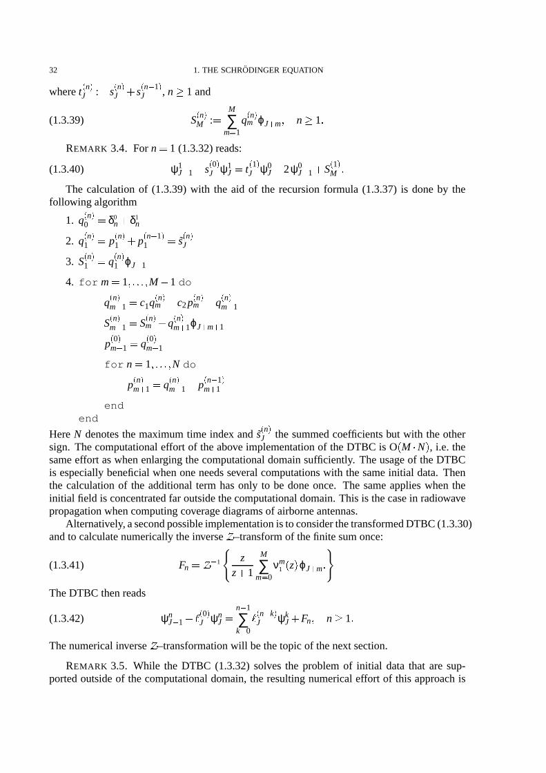
3.3. Numerical Results. Herewe presentthe numericalresultswhenusingour new dis-creteTBC (1.3.32)for the Schrodingerequation(1.1.1). We usethe sameinitial dataas inSection2.5, but shiftedsuchthat it is partially outsidethe computationaldomain0 x L.Again,dueto its construction,our DTBC yieldsexactly (up to round–off errors)thenumericalwhole–spacesolutionrestrictedto thecomputationalinterval 0 L .
Example. This exampleshows a simulationof a right travelling Gaussianbeam ψI x exp
i100x 30
x 0
8 2? at threeconsecutivetimesevolving underthefreeSchrodingerequa-
tion ( 1) with the rathercoarsediscretizationof 161grid pointsfor the interval 0 x 1(i.e.∆x 1% 160)andthetimestep∆t 2 9 10 5. For theright exterior (computational)domainwe choosethesamespacestep∆x anduse60 grid pointswhich resultsin theexterior interval1 x 1
38125.
In thefollowing Figure1.9we plottedtheabsolutevalueof theinitial dataandthesolutionobtainedwith thediscreteTBCs(1.3.32)at thetimestepst 0
002,t 0
004,t 0
006.One
clearly seesin Figure1.9 that the solution is solely propagatedto the right andno artificialreflectionsarecaused.
In this examplethecomputationusingthe inhomogeneousDTBCs(1.3.32)needsapprox-imatelythesameCPU–timethanjust enlarging thedomainto theinterval 0 x 1
8 usinga
simpleNeumannboundaryconditionat x 0 andx 18. FromFigure1.9onecanguessthat
thesolutionat t 0004hasalreadyreachedtheright boundaryat x 1
8. Henceit is worth-
while in thisexampleto usetheinhomogeneousDTBCswhenever thesolutionfor t 0004is
needed.
4. Numerical Inverse
–Transformations
Thecrucialpoint in thederivationof theDTBC in Section2 wasto find theexact inverse–transformations.If it is not possibleto calculatethe convolution coefficientsanalytically
thentheinverse
–transformationcanbeperformednumerically.Thenumericalinversionof the
–transformationis basedonthesimpleobservationthatthe
–transformationof thesequence- fn. , n 0 1 ? .
- fn. f
z : ∞
∑n) 0
fnz n z IC & z&3 R 1 (1.4.1)
is nothingelsebut a Taylor seriesin z 1% z, i.e. the problemof calculatingthe inverse
–transformationof f
z is the numericalevaluationof the Taylor coefficients of the function
fz : f
1% z . For thatpurposeweusedheretheFORTRAN subroutineENTCAF(Evaluation
of NormalizedTaylorCoefficientsof anAnalytic Function)from LynessandSande[C5].First we want to outline themethod.The (normalized)Taylor coefficientsrn fn canbeob-
tainedby Cauchy’s integral representation:
rn fn rn
2πi Q fz z n 1 dz r R(1.4.2)
where R denotesacirclearoundtheorigin with radiusr smallerthantheradiusof convergenceR of theTaylor series.Theapproximationto fn basedon usinganN–pointtrapezoidalrule for
34 1. THE SCHRODINGER EQUATION
0 0.1 0.2 0.3 0.4 0.5 0.6 0.7 0.8 0.9 10
0.1
0.2
0.3
0.4
0.5
0.6
0.7
0.8
0.9
1
x
|ψ|
Schroedinger: t=0
0 0.1 0.2 0.3 0.4 0.5 0.6 0.7 0.8 0.9 10
0.1
0.2
0.3
0.4
0.5
0.6
0.7
0.8
0.9
1
x
|ψ|
Schroedinger: t=0.002
0 0.1 0.2 0.3 0.4 0.5 0.6 0.7 0.8 0.9 10
0.1
0.2
0.3
0.4
0.5
0.6
0.7
0.8
0.9
1
x
|ψ|
Schroedinger: t=0.004
0 0.1 0.2 0.3 0.4 0.5 0.6 0.7 0.8 0.9 10
0.1
0.2
0.3
0.4
0.5
0.6
0.7
0.8
0.9
1
x
|ψ|
Schroedinger: t=0.006
FIGURE 1.9. Solution & ψ x t (& at time t 0, t 0
002,t 0
004,t 0
006:
thesolutionwith thenew discreteTBCs(1.3.32)coincideswith thewhole–spacesolutionanddoesnot introduceany numericalreflections.
thecontourintegral is f N n givenby
rn f N n 1
N
N 1
∑k) 0
e in 2πkN f rei 2πk
N n 0 1 ? N 1
(1.4.3)
Theapproximationrn f N n is obtainedby an iterative process.First approximationsf
N 0 , N
1 2 4 8 arecomputedusing(1.4.3). Theconvergencecriterion is basedon theknowledge
of theexactvalueof the limit of thesequence:limN : ∞ f N 0 f0 f
0 (cf. the Initial Value
TheoremZ.6 in theAppendix).After converging thesecondpartconsistsin evaluating(1.4.3)for n 0 1 ? N 1 usingthestoredfunction valuesobtainedin the first part. SinceN is apowerof 2 it is particularlyappropriateto usea fastFouriertransformtechniquefor this part.
Theuserhasto specifytherequiredabsoluteaccuracyεreq andtheradiusof computationr(theonly restrictionis that r mustbe lessthanR). ENTCAF returnsanaccuracyestimateεest

4. NUMERICAL INVERSE P –TRANSFORMATIONS 35
togetherwith approximationsrn f N n andanumberN, which aresupposedto satisfy
rn f N n rn fn εest n 0 1 2 N 1(1.4.4a)
& rn fn & εest n N N 1 ?4(1.4.4b)
Weseefrom(1.4.4a)thatthisalgorithmnaturallydeliversapproximationsrn f N n with auniform
boundon thediscretizationerror. An outputstatusparameterindicatesto theuserwhetherornot convergenceor roundoff errorshave occurred. Exploiting the informationof this outputparameteronecouldconstructadriverprogramwhichfindstheappropriatevalueof r by itself.
Due to the asymptoticbehaviour (1.2.36)it is not advisableto calculatethe0 n
j . Instead
we show how to computethesummedconvolution coefficientss nj numerically. Thes
nj were
definedby:
s nj : 0 n
j 0 n 1j n 1 s
0j 0 0
j j 0 J (1.4.5)
Weconcentrateon theright BC at j J. If weassumel 1j 0 wehave:
- s nJ
. ν2
z z 1ν2
z
1 z ν2
z(1.4.6)
with ν2
z ν2
z andν2
z givenby formula(1.2.21).
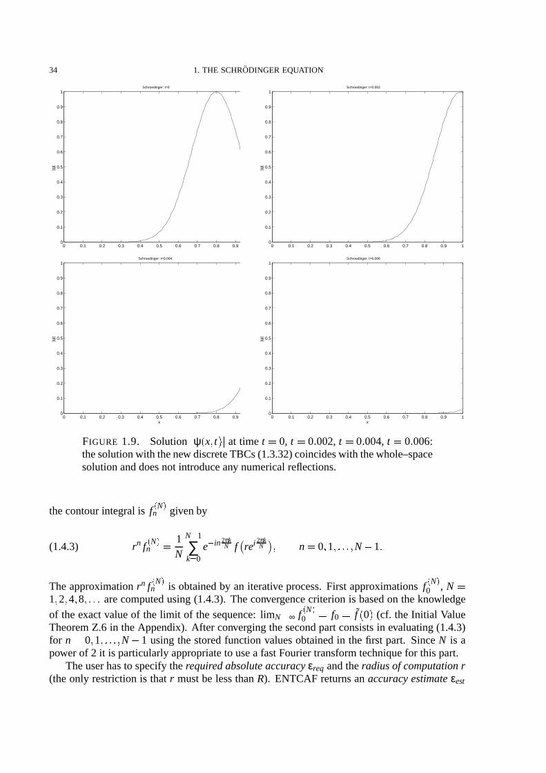
4.1. Numerical Results. Herewepresentthenumericalresultswhenusingthesubroutine
ENTCAF to computetheconvolution coefficients0 n
J , s nJ . In eachexamplewe choseεreq
10 6 andsetthemachineaccuracyparameterεM to 10 15.
Example1. Thevaluefor thepotentialVL wassetto 2 9 104 andthediscretizationparameterweretaken from the exampleof Subsection2.5, i.e. ∆x 1% 160,∆t 2 9 10 5. We usedthecomputationalradiusr 0
92. For thatparameterchoiceENTCAF returneda numberof N
256nontrivial calculatedcoefficientsandanestimateduniformabsoluteaccuracy εest 983029
10 7 in caseof thecoefficients0 n
J . For thesummedcoefficientss nJ weobtainedN 128and
εest 476849 10 7. In thefollowing Figure1.10wepresenttherealandimaginarypartof the
numericallyobtainedcoefficientsin comparisonto theexactvalues.
0 20 40 60 80 100 120 140 160 180−0.3
−0.2
−0.1
0
0.1
0.2
0.3
Re lJ(n)
n0 20 40 60 80 100 120 140 160 180
−20
−15
−10
−5
0
5
10
15
20
Im lJ(n)
n
FIGURE 1.10. Example1: Valuesfor Re0 n
J , Im0 n
J

36 1. THE SCHRODINGER EQUATION
One seriousproblemis the rescalingof the computedcoefficients. Sincethe algorithm
yieldsapproximationsrn f N n with auniformaccuracy (1.4.4a)thecomputationis only reliable
to a limited numberof n whencalculating f N n from rn f
N n for r 1. Thereforesomevisible
numericalerrorsoccurin thecalculationof Re0 n
J for n 130andIm0 n
J for n 170.On theleft sideof Figure1.10we observe thealternatingbehaviour shown in (1.2.36)
0 nj + 2iR
1 n i8
∆x 2
∆t
1 n i1258
1 n (1.4.7)
0 10 20 30 40 50 60 70 80 90−0.5
−0.4
−0.3
−0.2
−0.1
0
0.1
0.2
0.3
0.4
0.5
Re sJ(n)
n0 10 20 30 40 50 60 70 80 90
−0.2
−0.1
0
0.1
0.2
0.3
0.4
0.5
0.6
0.7
0.8
Im sJ(n)
n
FIGURE 1.11. Example1: Valuesfor Res nJ , Im s
nJ .
0 10 20 30 40 50 60 70 80 900
1
2
3
x 10−4 Error in Re l
J(n), Re s
J(n)
n
Error in Re lJ(n)
Error in Re sJ(n)
0 10 20 30 40 50 60 70 80 900
1
2x 10
−3 Error in Im lJ(n), Im s
J(n)
n
Error in Im lJ(n)
Error in Im sJ(n)
FIGURE 1.12. Example1: Dif ferencebetweenthenumericalandexactvalue
of therealandimaginarypartof0 n
J (—) ands nJ ( 999 ).
Example 2. In this secondexamplewe setthe potentialto zeroandchangedthe compu-tationalradiusto r 0
95 andthestepsizes∆x 1% 1600,∆t 2 9 10 4. For thecoefficients0 n
J ENTCAFreturnedanumberof N 256nontrivial calculatedcoefficientsandanestimated
uniform absoluteaccuracy εest 298029 10 6. In caseof the summedcoefficients s
nJ we
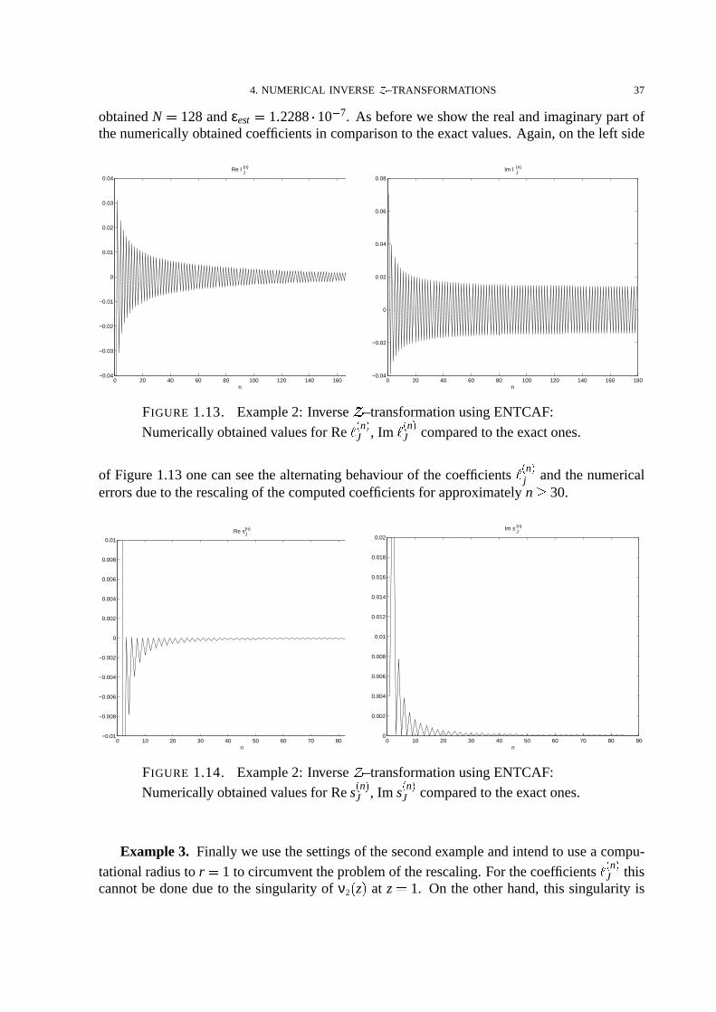
4. NUMERICAL INVERSE P –TRANSFORMATIONS 37
obtainedN 128andεest 122889 10 7. As beforewe show therealandimaginarypartof
thenumericallyobtainedcoefficientsin comparisonto theexactvalues.Again,on theleft side
0 20 40 60 80 100 120 140 160 180−0.04
−0.03
−0.02
−0.01
0
0.01
0.02
0.03
0.04
Re lJ(n)
n0 20 40 60 80 100 120 140 160 180
−0.04
−0.02
0
0.02
0.04
0.06
0.08
Im lJ(n)
n
FIGURE 1.13. Example2: Inverse
–transformationusingENTCAF:
Numericallyobtainedvaluesfor Re0 n
J , Im0 n
J comparedto theexactones.
of Figure1.13onecanseethealternatingbehaviour of thecoefficients0 n
j andthenumericalerrorsdueto therescalingof thecomputedcoefficientsfor approximatelyn 30.
0 10 20 30 40 50 60 70 80 90−0.01
−0.008
−0.006
−0.004
−0.002
0
0.002
0.004
0.006
0.008
0.01
Re sJ(n)
n0 10 20 30 40 50 60 70 80 90
0
0.002
0.004
0.006
0.008
0.01
0.012
0.014
0.016
0.018
0.02
Im sJ(n)
n
FIGURE 1.14. Example2: Inverse
–transformationusingENTCAF:
Numericallyobtainedvaluesfor Res nJ , Im s
nJ comparedto theexactones.
Example 3. Finally we usethesettingsof thesecondexampleandintendto usea compu-
tationalradiusto r 1 to circumventtheproblemof therescaling.For thecoefficients0 n
J thiscannotbe donedueto the singularityof ν2
z at z 1. On the otherhand,this singularity is

38 1. THE SCHRODINGER EQUATION
0 10 20 30 40 50 60 70 80 900
0.2
0.4
0.6
0.8
1
1.2x 10
−6 Error in Re lJ(n), Re s
J(n)
n0 10 20 30 40 50 60 70 80 90
0
0.2
0.4
0.6
0.8
1
1.2x 10
−6 Error in Im lJ(n), Im s
J(n)
n
FIGURE 1.15. Example2: Inverse
–transformationusingENTCAF:Differencebetweenthenumericalandexactvalueof therealandimaginarypart
of0 n
J (—) ands nJ ( 999 ).
removedin (1.4.6): - s nJ
. 1 z ν2
z
1 z iR2
y iR2 4i
R
1 z y y(1.4.8)
with theabbreviation y 1 z iκ
z 1 .
For thesummedcoefficientss nJ ENTCAFreturnedanumberof N 1024nontrivial calcu-
latedcoefficientsandanestimateduniformabsoluteaccuracy εest 224929 10 6. Themaximal
absoluteerrorfor Res nJ is 2
86099 10 6 and2
14559 10 6 for calculatingIm s
nJ .
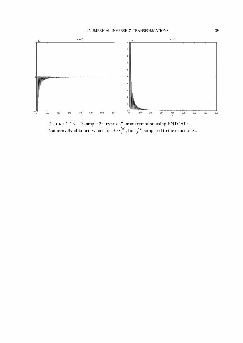
4. NUMERICAL INVERSE P –TRANSFORMATIONS 39
0 100 200 300 400 500 600 700 800−1
0
1x 10
−3 Re sJ(n)
n0 100 200 300 400 500 600 700 800
0
1
2
3
4
5
6
7
8
9
10x 10
−4 Im sJ(n)
n
FIGURE 1.16. Example3: Inverse
–transformationusingENTCAF:
Numericallyobtainedvaluesfor Res nJ , Im s
nJ comparedto theexactones.

40 1. THE SCHRODINGER EQUATION

CHAPTER 2
The Convection–DiffusionEquation
Herewewill demonstratehow thederivationof theDTBC of theprecedingChaptercarriesoverto thecaseof alinearconvection–diffusionequation.Thistypeof parabolicequationarisesfor examplein thestudyof heatconduction,reactiondiffusionproblemsandwhenlinearizingtheNavier–Stokesequation.Theresultswill begeneralizedto theθ–schemewith the implicit-nessparameter0 θ 1 andto aflexible discretizationof theconvectionterm.A shortversionof this Chaptercanbefoundin [P2]. This approachcanbegeneralizedto a vector–valuedpar-abolicequationdescribing(secondorder) fluid stochasticPetri nets[P7].
1. Transparent Boundary Conditions
In this Sectionwe shortly presentthe derivation of the (analytic)TBC. For simplicity ofthenotationwerestrictourselveshereto a constantcoefficientparabolicequationin onespacedimension:
ut auxx bux
cu x IR t 0ux 0 uI
x (2.1.1)
Of course,in generalthecoefficientsin (2.1.1)maydependon x andt but for our purposesweshall assumethat they remainconstantoutsideof the computationaldomain. Without lossofgeneralitywe assumefor the reactionratec 0 (otherwisethis propertycanbeachievedby achangeof variablesv uexp
ct ).1.1. Derivation of the TBC. Herewe determinetheTBCs at x 0 andx L, suchthat
the solution of the resulting IBVP coincideswith the solution of the whole–spaceproblem(2.1.1)restrictedto
0 L . Oncemorewehaveto assumethattheinitial datauI
x is compactly
supportedin thecomputationaldomain0 L . Proceedinganalogouslyto theformalderivation
of theTBCsin Chapter1 weconsiderthe interior problem
ut auxx bux
cu 0 x L t 0ux 0 uI
x
ux0 t
T0u 0 t ux
L t
TLu L t (2.1.2)
andobtaintheDirichlet–to–NeumannmapT0 by solvingthe left exterior problem:
vt avxx bvx
cv x 0 t 0vx 0 0
v0 t Φ
t t 0 Φ
0 0
v ∞ t 0T0Φ t vx
0 t
(2.1.3)
41

42 2. THE CONVECTION–DIFFUSIONEQUATION
(2.1.3)is coupledwith (2.1.1)by theassumptionthatu, ux arecontinuousacrosstheartificialboundaryat x 0. Sincethe initial datavanishesfor x 0, we cansolve (2.1.3)explicitly bytheLaplace–methodandobtainthetransformedleft exterior problem:
avxx bvx
c s v 0 x 0
v0 s Φ
s (2.1.4)
Thesolutionwhich decaysasx ∞ is simply vx s Φ
s eλ1 s x, x 0, with
λ1 2 s b2a
6 1!a ! η s(2.1.5)
andtheparameter
η b2
4a c 0
(2.1.6)
Consequently, thetransformedleft TBC reads:
ux0 s λ1
s u
0 s (2.1.7)
Weremindthereaderthatin (2.1.5) ! denotesthebranchof thesquarerootwith nonnegativerealpart.After theinverseLaplacetransformationthe left TBC reads:
ux0 t b
2au0 t 1!
aπe ηt d
dt
t
0
u0 τ eητ!
t τdτ
(2.1.8)
We observe againthat (2.1.8) is nonlocalin t (of memory–type),i.e. the computationof thesolutionat sometimeusesthesolutionat all previoustimes.Theright TBCat x L is derivedsimilarly:
uxL t b
2auL t 1!
aπe ηt d
dt
t
0
uL τ eητ!
t τdτ
(2.1.9)
REMARK 1.1(InhomogeneousEquation). We note that it is possibleto consider(2.1.1)with an inhomogeneityf
x t provided that f
x t f is constantoutsideof
0 L . In this
casethetransformedleft exterior problemis aninhomogeneousODE in x:
avxx bvx
c s v s 1 f x 0
v0 s Φ
s (2.1.10)
anda (constantin x) particular solutionreads
vpart x s fsc s x 0(2.1.11)
i.e. thegeneralsolutionto (2.1.10)is
vx s Φ
s f
sc s eλ1 s x f
sc s x 0(2.1.12)
with λ1
s givenin (2.1.5).Thereforethe transformedleft TBC is givenby:
vx0 s λ1
s Φ
s λ1
s f
c1s 1
c s(2.1.13)
andaftertheinverseLaplacetransformationthe left TBC reads:
ux0 t b
2au0 t ψ
t 1!
aπe ηt d
dt
t
0
u0 t ψ
t eητ!
t τdτ (2.1.14)

1. TRANSPARENT BOUNDARY CONDITIONS 43
whereψt is obtainedusing(IL.3):
ψt f
c
1 e ct (2.1.15)
1.2. Well–posednessof the IBVP. It is known thattheIVP (2.1.1)is well–posed:
THEOREM 2.1(Theorem6.2.1,[F8]). Theinitial valueproblemfor theequation(2.1.1)iswell–posed,i.e. for anytimeT 0 there is a constantCT such thatanysolutionu
x t satisfies
" u t (" L2 IR t
0" ux
τ (" L2 IR dτ CT " uI " L2 IR(2.1.16)
for 0 t T.
However, thewell–posednessof theassociatedIBVP is not cleara-priori. While theexis-tenceof a solutionto the1D parabolicequation(2.1.2)with theTBCs(2.1.9), (2.1.8)at x 0andx L is clearfrom theusedconstructionit remainsto provetheuniquenessof thesolution.A straightforwardcalculationusingtheenergy method,i.e.multiplying (2.1.1)with u
x t and
integratingby partsin x, yields
12
ddt
" u t (" 2L2 0 L a " u S t (" 2
L2 0 L bL
0ux t ux
x t dx c " u t #" 2
L2 0 L au
x t ux
x t (& x) L
x) 0
aux t ux
x t (& x) L
x) 0 (2.1.17)
if c b2 % 4a (which canalwaysbe achieved by a changeof variables).Finally, integrating
in time usingPlancherel’s Theoremfor theLaplacetransformation(TheoremL.3) (u0 t and
uL t areextendedby 0 for t T) gives
" u t (" L2 0 L I" uI " L2 0 L 2aT
0 u
L t uxL t u
0 t ux
0 t dt
" uI " L2 0 L 2aIR
λ2
iξ '& u
L iξ (& 2 λ1
iξ '& u
0 iξ (& 2 dξ
" uI " L2 0 L 4a∞
0Reλ2
iξ '& u
L iξ (& 2 Reλ1
iξ '& u
0 iξ (& 2 dξ
(2.1.18)
sinceu0 iξ ¯u
0 iξ , u
L iξ ¯u
L iξ , λ1 2 L iξ λ1 2 L iξ . Now it caneasilybe
checkedthattheconditionsfor well–posedness
Reλ1
iξ 0 for ξ IR(2.1.19a)
Reλ2
iξ 0 for ξ IR(2.1.19b)
(λ1 2 givenby (2.1.5))arefulfilled andwecanstatethefollowing theorem.
THEOREM 2.2. Theresultingparabolic IBVP is well–posed
" u t #" L2 0 L *" uI " L2 0 L t 0(2.1.20)
andthis impliesuniquenessof thesolutionto theparabolicIBVP.

44 2. THE CONVECTION–DIFFUSIONEQUATION
2. DiscreteTransparent Boundary Conditions
Next weshalladdressthequestionhow to adequatelydiscretizetheanalyticTBC (2.1.8)fora chosenfull discretizationof (2.1.1). Insteadof discretizingtheanalyticTBC (2.1.8)with itssingularitywe derive thediscreteTBCsof thefully discretizedproblembasedon theso–calledweightedaverageor θ–schemefor 0 θ 1. With theuniform grid pointsx j j∆x tn n∆tandtheapproximationun
j / ux j tn theθ–schemefor solving(2.1.1)reads:
Dt unj aD2
xun θj
bDσxun θ
j cun θ
j (2.2.1)
with
un θj θun 1
j 1 θ un
j 0 θ 1
(2.2.2)
REMARK 2.1. While a uniform grid in x is necessaryin the exterior domain,the interiorgrid maybenonuniformin x.
In the scheme(2.2.1) Dt denotesthe usualforward and D2x the secondorder difference
quotient:
Dt unj un 1
j un
j
∆t D2
xun θj un θ
j 1 2un θ
j un θj 1
∆x 2
(2.2.3)
The convectionterm is discretizedby the parametrizeddifferencequotientDσx σDx
1 σ D @x , i.e.
Dσxun
j σunj 1
1 2σ unj
1 σ unj 1
∆t 0 σ 1(2.2.4)
which allows to switchbetweenacentereddifferencequotient(σ 1% 2) or aone–sideddiffer-encequotient(σ 0 or σ 1).
REMARK 2.2(“upwind differencing”). Onetypicalpropertyof theparabolicequation(2.1.1)is that
supx, IR
& u x t (& sup
x , IRux t < if t t <
Thatis, themaximumvalueof & u x t (& will not increaseast increases(“maximumprinciple” ).
In [D10, Chapter4.1.6] it wasproven that the differencescheme(2.2.1) will have a similarpropertyif andonly if thetwo conditions
σb∆xa
1 and1 σ b∆x
a 1(2.2.5)
aresatisfied.Wenotethatfor areasonablechoiceof σ (”upwind differencing”),i.e.0 σ 1% 2for b 0 and1% 2 σ 1 for b 0 theseconditionscanalwaysbefulfilled.
REMARK 2.3(stabilityof thescheme). Secondlyonecaneasilyshow usingthevon–Neu-mannanalysis[F8] that the differencescheme(2.2.1) for solving the initial value problem(2.1.1)is stable(in thediscreteL2–norm)providedthatthestability condition
1 2θ a
∆t∆x 2 1(2.2.6)
holdsandupwinddifferencingis used.I.e. for a ratherimplicit scheme(θ 1% 2) noadditionalconditionhasto beimposedto ensurestability.

2. DISCRETETRANSPARENT BOUNDARY CONDITIONS 45
2.1. Discretization strategiesfor the TBC. Herewe want to comparethreestrategiestodiscretizethe TBC (2.1.8) which is a ratherdelicatequestion. First we review two knowndiscretizationtechniquesfrom Mayfield [T16] andHalpern[P3].
DiscretizedTBC of Mayfield. To compareourresultswefirst repeatthead-hocdiscretiza-tion strategy of Mayfield appliedto the convection–diffusion equation. Accordingto the ap-proachof Mayfield [T16] for theSchrodingerequationoneway to discretizetheanalyticTBC(2.1.8)at x 0 in theequivalentform
u0 t a
π
t
0
ux0 τ e η t τ !
t τdτ b
2!
aπ
t
0
u0 τ e η t τ !
t τdτ (2.2.7)
is for thefirst integral
t
0
ux0 t τ e ητ!
τdτ / 1
∆x
n 1
∑m) 0
un m
1 un m
0 e ηm∆ttm 1
tm
dτ!τ
2!
∆t∆x
n 1
∑m) 0
un m
1 un m
0 e ηm∆t!m 1 !
m
(2.2.8)
Discretizingthe secondintegral in (2.2.7)analogouslyleadsto the following discretizedTBCfor theconvection–diffusionequation:
un1 1 b
2aun
0 !
π∆x
2!
a∆tun
0 n 1
∑m) 1
un m
1 un m
0 ˜0 m b2a
n 1
∑m) 1
un m0
˜0 m(2.2.9)
with theconvolutioncoefficientsgivenby
˜0 m e ηm∆t!m 1 !
m
andη definedby (2.1.6).Onthefully discretelevel (2.2.9)is notperfectlytransparentany moreandmaypossiblyleadto anunstablenumericalschemeasshown in Theorem1.2in caseof theSchrodingerequation.
REMARK 2.4(AlternativeDiscretizationof theTBC). In thecontext of underwateracous-ticsThomsonandMayfield [T26] proposedanalternativediscretizationof (2.1.8)to handletheexponentialtermsmoreaccuratelywhenη
t τ is large. This approachwill bepresentedin
Chapter3.
Artificial BC of Halpern. Secondlywe presenttheapproach of Halpern [P3] which wasgeneralizedby Loheacin [P5], [P6] to the casethat the diffusion coefficient a in (2.1.1)candependon x. HalpernandRauchderivedin [P4] absorbingboundaryconditionswith variablecoefficients,curved artificial boundaryandarbitraryconvection. The numericalstudyof thisconditionswerecarriedout in [P1] by Dubach.
In [P3]Halperndevelopedafamilyof artificial boundaryconditionsfor thelinearconvection–diffusion equationwith small diffusion a. To startwith we rewrite the transformedleft TBC(2.1.7)as
ux0 s 1
2ab b2 4
c s a u
0 s (2.2.10)

46 2. THE CONVECTION–DIFFUSIONEQUATION
Now Halpern’sapproachconsistsof usingTaylor or Padeapproximationsof thetermin paren-thesesin (2.2.10)with respectto a small valueof a in order to obtaina local in t boundarycondition.A first orderTaylorapproximationgives
b b2 4c s a / b & b & 2a
c s& b & (2.2.11)
which leadsto thetransformedboundarycondition
ux0 s b & b &
2a c s& b & u
0 s (2.2.12)
Finally an inverseLaplacetransformationyields (dependingon the sign of b) the first orderartificial boundaryconditions:
inflow BCb 0 : ut
0 t bux
0 t b2
a c u0 t 0(2.2.13a)
outflow BCb 0 : ut
0 t bux
0 t cu
0 t 0
(2.2.13b)
To discretize(2.2.13)we follow thesuggestionin [P3] andgeneralizeit for theθ–scheme:
inflow BCb 0 : Dt un
0 bDxun θ
0 b2
a c un θ0 0(2.2.14a)
outflow BCb 0 : Dt un
0 bDxun θ0 cun θ
0 0(2.2.14b)
and analogouslyat the right boundaryat L J∆x. While Halpernshowed that the interior(Crank–Nicolson)schemetogetherwith theabsorbingboundarycondition(2.2.14)(for c 0) isstableandhasordertwo in timeandspace,theresultingschemesuffersfrom reducedaccuracyaswewill seelaterin thenumericalexamplesof Section3.
Discrete TBC. In orderto avoid any numericalreflectionsat the boundaryandto ensureunconditionalstabilityof theresultingschemewewill constructdiscreteTBCsinsteadof choos-ing anad–hocdiscretizationof theanalyticTBC (2.1.8)like(1.2.7)or theapproachof Halpern.ThediscreteTBCscompletelyavoid any numericalreflectionsat theboundaryat noadditionalcomputationalcosts(comparedto (2.2.9)).
2.2. Derivation of the DTBC. Wemimic thederivationfrom Section1 onadiscretelevel:we obtaintheDTBC by solvingthediscreteleft exterior problem, i.e. (2.2.1)for j 1:
∆t unj b
∆t∆x
σ∆x 1 σ ∆ @x un θ
j 2κun θj r∆2
xun θj (2.2.15)
wherer a∆t % ∆x 2 denotesthe(parabolic)meshratio, κ c∆t % 2 andσ denotestheparam-
eterexplainedin (2.2.4). In thescheme(2.2.15)we usedthedifferenceoperators∆t ∆t Dt ,∆2
x ∆x 2D2
x, etc.Oncemoreweapplythe
–transformation: - un
j. u j
z : ∑∞
n) 0unj z n,
j fixed,to solve (2.2.15)explicitly. We assumefor theinitial datau0j 0 j 2 andobtainthe
transformedscheme
1r
z 1θz 1 θ
u jz τ ∆x τ @ ∆ @x 2κ
ru j
z ∆2
xu jz j 1(2.2.16)
with
τ σb∆xa
τ @ 1 σ b∆x
a
(2.2.17)

2. DISCRETETRANSPARENT BOUNDARY CONDITIONS 47
Thetwo linearlyindependentsolutionsof theresultingsecondorderdifferenceequation(2.2.16)take theform
u jz ν j 1
1 2 z j 1(2.2.18)
whereν1 2 z arethesolutionsof thequadraticequation
ν2 21 τ 1 1
rz 1
2θz 1 θ κ τ τ @
2ν 1 τ @
1 τ 0
(2.2.19)
Sincewe areseekingdecreasingmodesas j ∞ we have to require & ν1
z(&B 1 andobtain
the
–transformedleft discreteTBCas
u1
z ν1
z u0
z (2.2.20a)
Analogously, the
–transformedright discreteTBC reads
uJ 1z 1 τ
1 τ @ ν1
z uJ
z(2.2.20b)
wherewehaveusedthepropertyν1
z ν2
z
1 τ @ % 1 τ .
REMARK 2.5. It wasshown by Lill [D4, Theorem3.11] that for the solutionsto thequa-draticequation(2.2.19) & ν1
z#&A 1, & ν2
z(&A 1 holdsfor & z&A 1.
It only remainsto inverse
–transformν1
z in order to obtain the discreteTBCs from
(2.2.20)andin a tediouscalculationthis canbeperformedexplicitly:
CALCULATION (of1 τ 1 - ν1
z . ). Firstwereformulate
1 τ ν1 2 z appropriately:
1 τ ν1 2 z 1 τ τ @
2 κr 1
rz 1
2θz 1 θ
6 1 1r
z 12θz 1 θ κ τ τ @
2
2 1 τ @ 1 τ
H κr 1
21 θ
1r
1θ
z
z 1 θθ
1 6 1r
! Az2 2Bz C2θz 1 θ
HerePe b∆x%
2a denotesthecell Pecletnumber. Theconstantscanbedeterminedas
A κ 2 4rθHκ
β 2 (2.2.21a)
B κ κ @ 2rH1 θ κ θκ @ β β @((2.2.21b)
C κ @ 2 4r
1 θ Hκ @
β @ 2 (2.2.21c)
with theabbreviations
κ 1 2θκ 1 θc∆t (2.2.22a)
κ @ 1 21 θ κ 1
1 θ c∆t (2.2.22b)
β θb∆t∆x
β @ 1 θ b∆t
∆x(2.2.22c)
H 1 1 2σ Pe
(2.2.22d)
We notethat for a reasonablechoiceof σ (”upwind differencing”),i.e. 0 σ 1% 2 for b 0and1% 2 σ 1 for b 0,
1 2σ Pe 0 holds andconsequentlyH 1 and A is always
positive. Thiswill beassumedfrom now on.

48 2. THE CONVECTION–DIFFUSIONEQUATION
For theinverse
–transformationweuseagain(1.2.23)andobtain
! Az2 2Bz C2θz 1 θ 1!
A
Az2 2Bz C2z
θz 1 θ F
λz µ
1!A
A2θ C
21 θ
1z
E2θz 1 θ F
λz µ
with E givenby
E 1 θθ
A 2B θ1 θ
C
(2.2.23)
Now applyingtheinversionrules(especially(IZ.9)) givenin theAppendixyieldsfor 0 θ 1:
1 ! Az2 2Bz C2θz 1 θ 1!
A
A2θ
δ0n C
21 θ δ1
n
E21 θ 1 θ
θn δ0
n 1 Pnµ
1!A
A2θ
Pnµ C
21 θ Pn 1
µ
E21 θ
n 1
∑k) 0
1 θθ
n kPk
µ
where 1 denotesthediscreteconvolution. Finally, weobtainwith (IZ.10)1 τ 1 - ν1 2 z . H κ
r 1
21 θ r δ0
n 1 n
2θ1 θ r
1 θθ
n
6 1
r!
A
A2θ
Pnµ C
21 θ Pn 1
µ
12θ
1 θ 2
n 1
∑k) 0
1 θθ
n kPk
µ
(2.2.24)
sincetheconstantE canbesimplydeterminedfrom (2.2.23)as
E 1θ1 θ
(2.2.25)
We recallfrom Chapter1 thattheparametersλ, µ aregivenby
λ !
A
! C µ B!
A ! C
(2.2.26)
It caneasilyseenfrom (2.2.21)thatthefollowing relationshold:
C A 4rH 2c∆t 1 2θ 4rHc∆t
c∆t 2 b∆t∆x
2 (2.2.27)
B2 AC 2r 2 H2 Pe
2 (2.2.28)
For C 0, i.e. if f
H2 Pe2 H 1
21 θ r c
∆x 2
2a
2 (2.2.29)
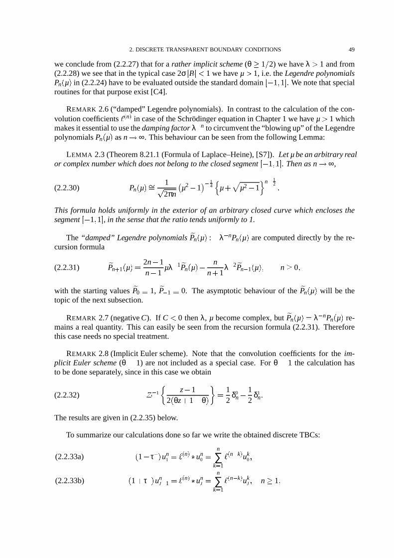
2. DISCRETETRANSPARENT BOUNDARY CONDITIONS 49
we concludefrom (2.2.27)thatfor a ratherimplicit scheme(θ 1% 2) we have λ 1 andfrom(2.2.28)weseethatin thetypical case2σ & Pe &3 1 wehaveµ 1, i.e. theLegendrepolynomialsPn
µ in (2.2.24)haveto beevaluatedoutsidethestandarddomain 1 1 . Wenotethatspecial
routinesfor thatpurposeexist [C4].
REMARK 2.6(“damped”Legendrepolynomials). In contrastto thecalculationof thecon-volutioncoefficients
0 n in caseof theSchrodingerequationin Chapter1 wehaveµ 1 whichmakesit essentialto usethedampingfactorλ n to circumventthe“blowingup” of theLegendrepolynomialsPn
µ asn ∞. Thisbehaviour canbeseenfrom thefollowing Lemma:
LEMMA 2.3(Theorem8.21.1(Formulaof Laplace–Heine),[S7]). Letµbeanarbitraryrealor complex numberwhich doesnotbelongto theclosedsegment 1 1 . Thenasn ∞,
Pnµ+ 1!
2πnµ2 1 1
4 µ µ2 1n 1
2 (2.2.30)
This formula holdsuniformly in the exterior of an arbitrary closedcurvewhich enclosesthesegment 1 1 , in thesensethat theratio tendsuniformlyto 1.
The “damped” Legendre polynomialsPnµ : λ nPn
µ arecomputeddirectly by the re-
cursionformula
Pn 1µ 2n 1
n 1µλ 1Pn
µ n
n 1λ 2Pn 1
µ n 0(2.2.31)
with the startingvaluesP0 ; 1, P 1 ; 0. The asymptoticbehaviour of the Pnµ will be the
topicof thenext subsection.
REMARK 2.7(negativeC). If C 0 thenλ, µ becomecomplex, but Pnµ λ nPn
µ re-
mainsa realquantity. This caneasilybeseenfrom the recursionformula (2.2.31). Thereforethis caseneedsnospecialtreatment.
REMARK 2.8(Implicit Eulerscheme). Note that the convolution coefficients for the im-plicit Euler scheme(θ 1) arenot includedasa specialcase.For θ 1 the calculationhasto bedoneseparately, sincein this caseweobtain
1 z 12θz 1 θ 1
2δ0
n 1
2δ1
n
(2.2.32)
Theresultsaregivenin (2.2.35)below.
To summarizeour calculationsdonesofar wewrite theobtaineddiscreteTBCs:
1 τ un
1 0 n 1 un0 n
∑k) 1
0 n k uk0 (2.2.33a)
1 τ @J un
J 1 0 n 1 unJ n
∑k) 1
0 n k ukJ n 1(2.2.33b)

50 2. THE CONVECTION–DIFFUSIONEQUATION
with convolutioncoefficients0 n for 0 θ 1 givenby
0 0 H κr 1 !
A2θr0 n
1 n
2θ1 θ r
1 θθ
n 1
r!
A9
9 A2θ
Pnµ C
21 θ Pn 1
µ 1
2θ1 θ 2
n 1
∑k) 0
1 θθ
n kPk
µ
(2.2.34)
for n 1, andin thecaseθ 1:
0 0 H κr 1 !
A2r
0 1 1
2r 1
2r!
AAP1
µ 2B 1
2r1 B!
A
0 n 1
2r!
AAPn
µ 2BPn 1
µ CPn 2
µ n 2
(2.2.35)
wherePnµ : λ nPn
µ denotesthe“damped” Legendrepolynomialsandδ0
n is theKroneckersymbol.
REMARK 2.9(Explicit Eulerscheme). Thecalculationabovedoesnot work directly in thecaseof the explicit Euler scheme(θ 0) sincethe inverse
–transformationof ν1
z does
not exist. In this situationwe useinsteadof (2.2.20)the
–transformeddiscreteTBCs in theformulation
z 1u1
z z 1ν1
z u0
z(2.2.36a)
z 1uJ 1z 1 τ
1 τ @ z 1ν1
z uJ
z (2.2.36b)
To derive theconvolutioncoefficientsof theDTBC weconsider
1 τ z 1ν1
z H κ
rz 1 1
2rz 1
z 12r
! Az2 2Bz Cz
12r H κ
r 1
2rz 1 A 2Bz 1 Cz 2
2r!
AF
λz µ
(2.2.37)
andcalculate 1 τ 1 z 1ν1
z 1
2rδ0
n H κr
12r
δ1n
1
2r!
AAPn
µ 2BPn 1
µ CPn 2
µ (2.2.38)
Finally, weobtainthefollowing discreteTBCsfor theexplicit Eulerscheme:
0 0 un0
1 τ un 11
n 1
∑k) 1
0 n k uk0 (2.2.39a)
0 0 unJ
1 τ @J un 1J 1
n 1
∑k) 1
0 n k ukJ n 1(2.2.39b)

2. DISCRETETRANSPARENT BOUNDARY CONDITIONS 51
with convolutioncoefficients0 n givenby
0 0 1 !A
2r
0 1 H κr
12r
1 B!A
0 n 1
2r!
AAPn
µ 2BPn 1
µ CPn 2
µ n 2
(2.2.40)
2.3. The Asymptotic Behaviour of the Convolution Coefficients. In this subsectionwewantto investigatetheasymptoticbehaviour of theconvolutioncoefficients
0 n givenby (2.2.33).As in Chapter1 wewill seethatit is beneficialto reformulatetheDTBC (2.2.33).
Thesummedconvolution coeffcients. It followsimmediatelyfromLemma2.3thatlimn: ∞Pn
µ 0 holds.Thusthecoefficientshave thefollowing asymptoticbehaviour for n ∞:
0 n 1 n
2θ1 θ r
1 θθ
n + 1 n
2rθ1 θ 2
!A
1 θθ
n n 1
∑k) 0
θ1 θ
kPk
µ (2.2.41)
Using
limn: ∞
1!A
n 1
∑k) 0
θ1 θ
kPk
µ 1!
A
1
1 2 θ1 θµλ 1 θ
1 θ 2λ 2
1
A 2 θ1 θB θ
1 θ 2C
1
θ1 θ E
1 θ
(2.2.42)
in (2.2.41)wefinally obtain
0 n + 1 n
θ1 θ r
1 θθ
n 0 θ 1 as n ∞
(2.2.43)
In the specialcaseof the Crank–Nicolsonscheme(θ 1% 2) we get0 n + 4
1 n % r. Thisalternatingbehaviour (2.2.43)may leadto subtractive cancellationin (2.2.33). Thereforewepreferto usethefollowing (weighted)summedcoefficientsin theimplementation
s n : θ
0 n 1 θ 0 n 1 n 1 s
0 : θ0 0 0 θ 1(2.2.44)
andcomputewith thehelpof (2.2.23)
s n 1
r!
A
A2
Pnµ 1 θ
θA2 θ
1 θC2
12θ
1 θ Pn 1
µ C
2Pn 2
µ
1
2r!
AAPn
µ 2BPn 1
µ CPn 2
µ
!
A2r
Pnµ 2µλ 1Pn 1
µ λ 2Pn 2
µ
(2.2.45)
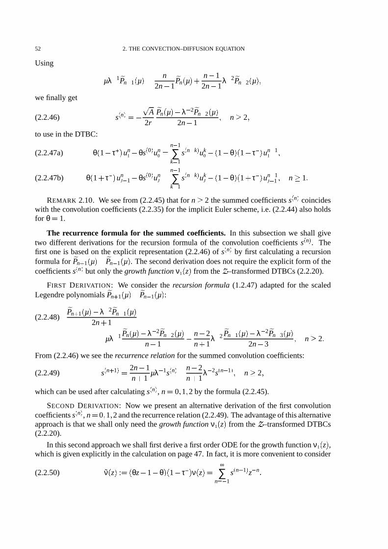
52 2. THE CONVECTION–DIFFUSIONEQUATION
Using
µλ 1Pn 1µ n
2n 1Pn
µ n 1
2n 1λ 2Pn 2
µ
we finally get
s n !
A2r
Pnµ λ 2Pn 2
µ
2n 1 n 2(2.2.46)
to usein theDTBC:
θ1 τ un
1 θs
0 un0 n 1
∑k) 1
s n k uk
0
1 θ 1 τ un 11 (2.2.47a)
θ1 τ @ un
J 1 θs
0 unJ n 1
∑k) 1
s n k uk
J
1 θ 1 τ @ un 1J 1 n 1
(2.2.47b)
REMARK 2.10. We seefrom (2.2.45)thatfor n 2 thesummedcoefficientss n coincideswith theconvolution coefficients(2.2.35)for theimplicit Eulerscheme,i.e. (2.2.44)alsoholdsfor θ 1.
The recurrenceformula for the summedcoefficients. In this subsectionwe shall givetwo different derivationsfor the recursionformula of the convolution coefficients s n . Thefirst oneis basedon theexplicit representation(2.2.46)of s n by first calculatinga recursionformulafor Pn 1
µ Pn 1
µ . Thesecondderivationdoesnot requiretheexplicit form of the
coefficientss n but only thegrowthfunctionν1
z from the
–transformedDTBCs(2.2.20).
FIRST DERIVATION: We considerthe recursion formula (1.2.47)adaptedfor the scaledLegendrepolynomialsPn 1
µ Pn 1
µ :
(2.2.48)Pn 1
µ λ 2Pn 1
µ
2n 1 µλ 1Pn
µ λ 2Pn 2
µ
n 1 n 2
n 1λ 2Pn 1
µ λ 2Pn 3
µ
2n 3 n 2
From(2.2.46)weseetherecurrencerelation for thesummedconvolutioncoefficients:
s n 1 2n 1
n 1µλ 1s
n n 2n 1
λ 2s n 1 n 2(2.2.49)
which canbeusedaftercalculatings n , n 0 1 2 by theformula(2.2.45).
SECOND DERIVATION: Now we presentan alternative derivation of the first convolutioncoefficientss n , n 0 1 2andtherecurrencerelation(2.2.49). Theadvantageof thisalternativeapproachis thatwe shallonly needthegrowthfunctionν1
z from the
–transformedDTBCs
(2.2.20).
In thissecondapproachweshallfirst deriveafirst orderODEfor thegrowth functionν1
z ,
which is givenexplicitly in thecalculationonpage47. In fact,it is moreconvenientto consider
νz :
θz 1 θ 1 τ ν z ∞
∑n) 1
s n 1 z n (2.2.50)

2. DISCRETETRANSPARENT BOUNDARY CONDITIONS 53
Usingtheconstants(2.2.21)and(2.2.22d)it hastheexplicit form
ν1 2 z z θ H κr 1
2r 1 θ H κ
r 1
2r6 1
2r Az2 2Bz C
(2.2.51)
Here,thesignhasto befixedsuchthat & ν1
z(&= 1 holds. This canbedonefor e.g.for z ∞.
Multiplying ν< dνdz
by Az2 2Bz C thenyields an inhomogeneousfirst orderODE for
νz :
AB
z2 2z CB
ν< z AB
z 1 νz β
z : β 1 z β 0 (2.2.52)
with
β 1 AB
1 θ H κ
r 1
2r θ H κr 1
2r
β 0 1 θ H κ
r 1
2r CB
θ H κr 1
2r
(2.2.53)
Its generalsolutionincludesν1 2 z asdefinedin (2.2.51). Recallingfrom (2.2.26)thatA% B λ % µ, C % B 1%
λµ holdsandusingtheLaurentseries(2.2.50)of ν andν< in (2.2.52)immedi-atelyyieldsthedesiredrecursionfor thecoefficientss n :
λµ
s 1 s
0 β 1 2
λµ
s 2 s
1 1λµ
s 0 β 0
n 1 s n 1
2n 1 µλ
s n
n 2 1λ2s
n 1 0 n 2(2.2.54)
whichcoincideswith (2.2.49).We remarkthat the startingcoefficient of the recursion(cf. (2.2.34))can be determined
with [S3,Theorem39.1]:
s 0 θ
0 0 limz: ∞
ν1
z
z θ H κr 1 !
A2r
0 θ 1
STABILITY OF THE RECURRENCE RELATION: For investigatingwhetherthe recurrencerelation (2.2.49)is well–conditionedwe proceedsimilar to Subsection2.3 in Chapter1 andwrite (2.2.49)asthesecondorderdifferenceequation
s n 1 a
n s n b n s n 1 0 n 3(2.2.55)
with thecoefficients
a n 2n 1
n 1µλ 1 b
n n 2n 1
λ 2 > 0
(2.2.56)
Therearetwo linearlyindependentsolutionss n1 , s
n2 to (2.2.55). To provethat(2.2.49)is well–
conditionedwe have to show that theseekedsolutionis not a minimalsolutionto (2.2.55),i.e.is adominantsolution.
Sincethecoefficientsa n , b n in (2.2.55)have thefinite limits
a limn: ∞
a n 2µλ 1 2
BA
b limn: ∞
b n λ 2 C
A > 0(2.2.57)
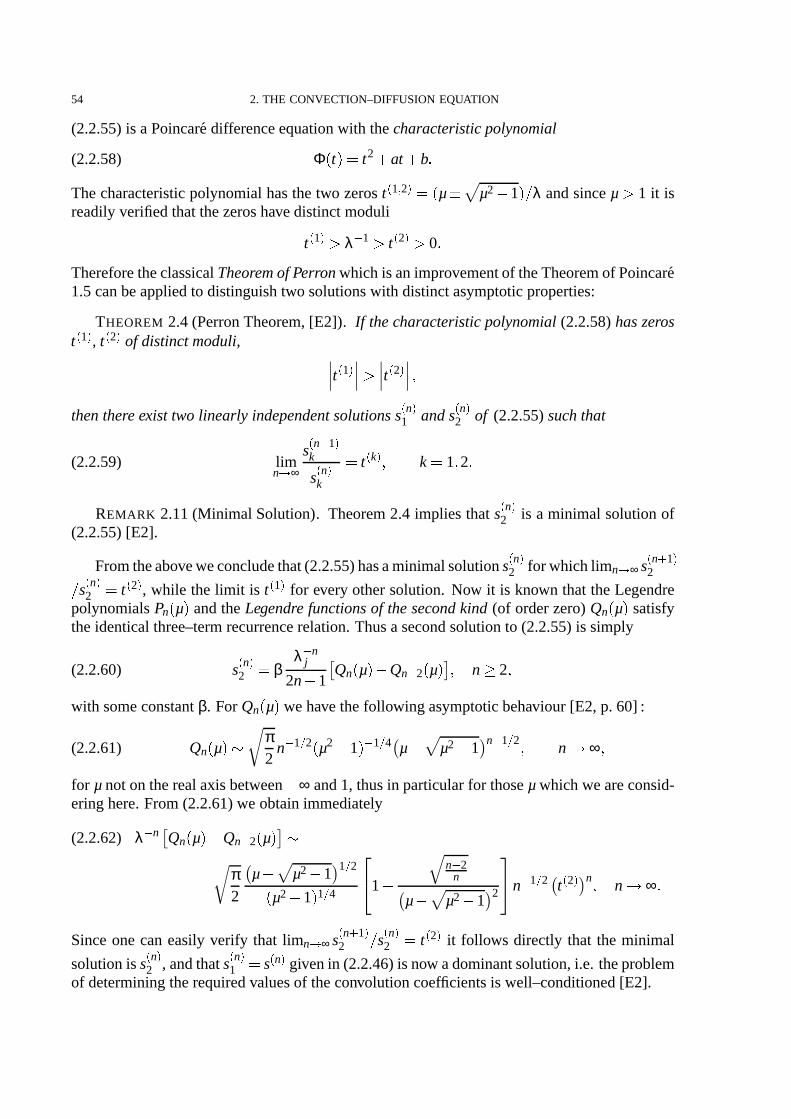
54 2. THE CONVECTION–DIFFUSIONEQUATION
(2.2.55)is aPoincare differenceequationwith thecharacteristicpolynomial
Φt t2 at b
(2.2.58)
Thecharacteristicpolynomialhasthetwo zerost 1 2 µ 6 µ2 1% λ andsinceµ 1 it is
readilyverifiedthatthezeroshavedistinctmoduli
t 1 λ 1 t
2 0
ThereforetheclassicalTheoremof Perronwhichis animprovementof theTheoremof Poincare1.5canbeappliedto distinguishtwo solutionswith distinctasymptoticproperties:
THEOREM 2.4(PerronTheorem,[E2]). If thecharacteristicpolynomial(2.2.58)haszerost 1 , t 2 of distinctmoduli,
t 1 t
2 thenthereexist two linearly independentsolutionss
n1 ands
n2 of (2.2.55)such that
limn: ∞
s n 1k
s nk
t k k 1 2
(2.2.59)
REMARK 2.11(Minimal Solution). Theorem2.4 implies thats n2 is a minimal solutionof
(2.2.55)[E2].
Fromtheaboveweconcludethat(2.2.55)hasaminimalsolutions n2 for whichlimn: ∞ s
n 12% s
n2 t 2 , while the limit is t 1 for every othersolution. Now it is known that theLegendre
polynomialsPnµ andtheLegendre functionsof thesecondkind (of orderzero)Qn
µ satisfy
theidenticalthree–termrecurrencerelation.Thusasecondsolutionto (2.2.55)is simply
s n2 β
λ nj
2n 1Qn
µ Qn 2
µ n 2(2.2.60)
with someconstantβ. For Qnµ wehave thefollowing asymptoticbehaviour [E2, p. 60] :
Qnµ + π
2n 1$ 2 µ2 1 1$ 4 µ µ2 1
n 1$ 2 n ∞ (2.2.61)
for µ noton therealaxisbetween ∞ and1, thusin particularfor thoseµ whichweareconsid-eringhere.From(2.2.61)we obtainimmediately
(2.2.62) λ n Qnµ Qn 2
µ +
π2
µ µ2 11$ 2
µ2 1 1$ 4 1 n 2n
µ µ2 1 2 n 1$ 2 t 2 n n ∞
Sinceonecaneasilyverify that limn: ∞ s n 12 % s
n2 t 2 it follows directly that the minimal
solutionis s n2 , andthats
n1 s n givenin (2.2.46)is now adominantsolution,i.e. theproblem
of determiningtherequiredvaluesof theconvolutioncoefficientsis well–conditioned[E2].

2. DISCRETETRANSPARENT BOUNDARY CONDITIONS 55
2.4. Stability of the resulting Scheme.To prove stability of the numericalschemewiththediscreteTBCs(2.2.47)weusethediscreteenergymethod. Weconcentrateonthecaseof theCrank–Nicolsonscheme(θ 1% 2) with centraldifferencingof theconvectionterm(σ 1% 2),i.e.weconsider(2.2.15)in theform
∆t unj r∆2
xun 1
2j
rPe∆0xu
n 12
j 2κu
n 12
j (2.2.63)
where∆0x ∆x ∆ @x denotesthe centereddifferenceoperator. We multiply theequationwith
un 1$ 2j andsumit up for the finite interior range j 1 2 ? J 1, using the summationby
partsrule (1.2.70):
J 1
∑j ) 1
un 1
j 2 un
j 2 2rJ 1
∑j ) 1
un 1
2j ∆2
xun 1
2j
2rPe
J 1
∑j ) 1
un 1
2j ∆0u
n 12
j 4κ
J 1
∑j ) 1
u
n 12
j 2
2rJ 1
∑j ) 0
∆xun 1
2j
2 2run 1
2J ∆ @xu
n 12
J 2ru
n 12
0 ∆xun 1
20
2rPeun 1
2J u
n 12
J 1 2rPeun 1
20 u
n 12
1 4κ
J 1
∑j ) 1
u
n 12
j 2
2run 1
2J 1 Pe un 1
2J 1
un 1
2J 2ru
n 12
0 1 Pe un 12
1 u
n 12
0
(2.2.64)
Finally asummationwith respectto thetimeindex yieldsthefollowing estimatefor thediscreteL2–norm(definedby " un " 2
2 : ∆x∑J 1j ) 1 & un
j & 2)
" uN 1 " 22 I" uI " 2
2 2a∆t
∆x
N
∑n) 0
un 1
2J
1 Pe un 1
2J 1
un 1
2J
N
∑n) 0
un 1
20
1 Pe un 1
21
un 1
20
I" uI " 22 2a∆t
∆x
N
∑n) 0
un 1
2J u
n 12
J 1 ˜0 n N
∑n) 0
un 1
20 u
n 12
0 1 ˜0 n
(2.2.65)
where ˜0 n : 0 n δ0n, j 0 J, givenin (2.2.33).
Again, asin the continuouscase,it remainsto show that the boundary–memory–termsin(2.2.65)areof positivetype. Weconcentrateon theboundarytermat j J anddefinethefinitesequences
fn un 1
2J 1 ˜0 n gn u
n 12
J n 0 1 N (2.2.66)
with fn gn 0 for n N, i.e. ∑Nn) 0 fngn 0 is to show. A
–transformationusing the
transformedDTBC (2.2.20)yields
- fn. f
z z 1
2uN
Jz
1 Pe ν1
z 1
12r
uNJz z 1 κ
z 1 6 Az2 2Bz C (2.2.67)

56 2. THE CONVECTION–DIFFUSIONEQUATION
whereuNJ
z ∑N
n) 0unJz n is analyticon & z&# 0. The zerosz1 2 of the squareroot above are
givenby z1 2 λ 1 µ 6 µ2 1 with λ, µ definedin (2.2.26). As remarkedon page48 in thetypicalcasewehaveλ 1, µ 1 andit canbeshown that0 z2 z1 1 holds.Theexpressionabove in thecurly bracketsis analyticfor & z&A z1 andcontinuousfor & z&A z1 andthereforef
z
is analyticon & z& z1. Notethatwehaveto choosethesignin (2.2.67)suchthatit matcheswithν1
z for & z& sufficiently large.For thesecondsequencegn weobtain
- gn. g
z z 1
2uN
Jz(2.2.68)
i.e. gz is analyticon & z&T 0. Now the basicideais to usePlancherel’s TheoremZ.4 which
gives:
N
∑n) 0
fngn 12π
2π
0fz g
z
z) eiϕdϕ
12π
π
0fz g
z f
z g
z
z) eiϕdϕ
1π
π
0Re f
z g
z
z) eiϕdϕ
(2.2.69)
wherewe have usedthe fact that fz f
z , g
z g
z , since fn gn IR. Using (2.2.67),
(2.2.68)weobtainN
∑n) 0
fngn 14π
π
0& z 1 & 2 uN
Jz 2
1 Pe Re- ν1
z . 1
z) eiϕdϕ
(2.2.70)
Weremarkthatthepoleof ν1
z atz 1 is “cancelled”by & z 1 & 2. From(2.2.70)weconclude
thatthediscreteL2–norm(2.2.65)is non–increasingin time if1 Pe Re- ν1
eiϕ . 1 0 D ϕ G 0 2π F(2.2.71)
holds. This propertyof ν1 can be shown in the following way. On the unit circle z eiϕ,0 ϕ 2π, wehave
z 1%
z 1 i tanϕ % 2 andthereby
yz : 1
rz 1z 1 κ 1
rκ i tan
ϕ2
0 ϕ 2π
(2.2.72)
Now ν1
z fulfils simply
1 Pe ν1
z 1 y
zU6 y
z 2 y
z Pe2(2.2.73)
andthereforeweobtaintherequestedproperty1 Pe Re- ν1
z . 1 κ
r Re yz 2 y
z Pe2 0(2.2.74)
for z eiϕ, 0 ϕ 2π.We thenhave thefollowing mainresultof thisSection:
THEOREM 2.5. Thenumericalschemewith theDTBCsis stablewith theproperty:
" un 1 " 2h : h
J 1
∑j ) 1
un 1j
2 *" u0 " 2h n 0
(2.2.75)

3. NUMERICAL RESULTS 57
Simplified DTBC. Therapiddecayof thes n On 3
2 motivatesto restrict(2.2.47)to aconvolutionover the“recentpast”(lastM time levels)asanoption:
θ1 τ un
1 θs
0 un0 n 1
∑k) n M
s n k uk
0
1 θ 1 τ un 11 (2.2.76a)
θ1 τ @B un
J 1 θs
0 unJ n 1
∑k) n M
s n k uk
J
1 θ 1 τ @J un 1J 1 n 1
(2.2.76b)
Wenotethatthestabilityof theresultingschemeis still notprovenyet.
3. Numerical Results
In theexamplesof thisSectionwewantto comparethenumericalresultsfromusingournewdiscreteTBC (2.2.47)to thesolutionusingeitherthediscretizedTBCof Mayfield[T26] or theapproximativeabsorbingBCof Halpern[P3]. Dueto its construction,ourDTBC yieldsexactly(up to round–off errors)the numericalwhole–spacesolution restrictedto the computationalinterval 0 L .
To measuretheinducederror(especiallyat theboundary)wecalculatea referencesolutionon a muchbiggerdomain(with DTBCs). The differencebetweenthe referencesolutionandthe computedsolution is called the reflectedpart. In eachexamplewe choose 0 1 as thecomputationaldomainandusethe initial data
uIx cos2 π
2x 0V 50V 45 for & x 0
5 &3 0
45
0 else(2.3.1)
Example 1. We usedthe parametersa 9, b 100, c 0, the time step∆t 10 4
andtherathercoarsespacegrid ∆x 1% 20 (which makesthedifferencein theaccuracy moreclear).Figure2.1shows thetime evolution of thesolutioncomputedwith theCrank–Nicolsonschemewith DTBCs at x 0, x 1 and σ 1% 2. Figure 2.2 shows the discreteL2–norm" un " 2 :
∆x∑J 1j ) 1 & un
j & 2 1$ 2 of the reflectedpart computedwith the Crank–Nicolsonschemewith the new DTBCs. and in Figure 2.3 one can seethe resultswhen using the boundaryconditionsof Mayfield and Halpernat x 0, x 1. This illustratesthe superiorityof ourdiscreteTBCs(2.2.47)(observe thedifferentscales!).
Thesimulationwith thediscretizedTBCs(2.2.9)from Mayfieldrequiresthesamenumericaleffort but thecomputedsolutionstronglydeviates(especiallyoncoarsegrids)from thewhole–spacesolution.Thediscretizationof Mayfield is convergent(if astabilityconditionis fulfilled).Thenumericalresultswith thefirst order boundarycondition(2.2.14)from Halpernarebetterthan the onewith (2.2.9) but worsethan the resultswith the simplifiedDTBC (2.2.76)withM 10,whichhasacomparablecomputationaleffort.
Example 2. In this examplewe usedagaintheCrank–Nicolsonschemeandcentraldiffer-encingof theconvectionterm: σ 1% 2. Now we useda finer grid thanbefore: the time step∆t 2 9 10 5 andthespacegrid ∆x 1% 160. We reducedthediffusivity: a 0
9, b 100,
c 0 andcomputedthesolutionuntil T 0014,i.e. 700time steps.Figure2.5demonstrates
oncemorethat usingour DTBC we obtain(up to round–off errors)the discretewhole–spacesolutionrestrictedto thecomputationalinterval.
Now we observe that the numericalresultswith the first orderBC (2.2.14)from Halpernarebetterthanbefore:weobtainapproximatelythesameerrorasthesimplifiedDTBC (2.2.76)

58 2. THE CONVECTION–DIFFUSIONEQUATION
t = 0
t = 0.002
t = 0.004
t = 0.006
t = 0.008
0 0.1 0.2 0.3 0.4 0.5 0.6 0.7 0.8 0.9 10
0.1
0.2
0.3
0.4
0.5
0.6
0.7
0.8
0.9
1
x
Evolution of Solution u
FIGURE 2.1. Example1: Temporalevolutionof thesolutionto (2.1.1)with theparametersa W 9, b WYX 100,c W 0.
discrete TBC
0 0.002 0.004 0.006 0.008 0.01 0.012 0.0140
0.5
1
1.5
2
2.5x 10
−16
time t
L^2−Norm of reflected Part
FIGURE 2.2. Example1: new DTBC: L2–norm of the reflectedpart (onlyroundoff–errorsoccur).

3. NUMERICAL RESULTS 59
discretized TBC
L. Halpern BC
discrete TBC: M=10
discrete TBC: M=20
0 0.002 0.004 0.006 0.008 0.01 0.012 0.0140
0.02
0.04
0.06
0.08
0.1
0.12
time t
L^2−Norm of reflected Part
FIGURE 2.3. Example1: OtherApproaches:L2–normof thereflectedpart.
t = 0
t = 0.002
t = 0.004
t = 0.006
t = 0.008
0 0.1 0.2 0.3 0.4 0.5 0.6 0.7 0.8 0.9 10
0.1
0.2
0.3
0.4
0.5
0.6
0.7
0.8
0.9
1
x
Evolution of Solution u
FIGURE 2.4. Example2: Temporalevolution of the solution to (2.1.1) witha W 0Z 9, b WYX 100,c W 0.

60 2. THE CONVECTION–DIFFUSIONEQUATION
0 0.002 0.004 0.006 0.008 0.01 0.012 0.0140
1
2x 10
−16
time t
DTBC: L^2−Norm of reflected Part
FIGURE 2.5. Example2: new DTBC: L2–norm of the reflectedpart (onlyroundoff–errorsoccur).
with M W 50 (seeFigure2.6). This is dueto thefiner discretizationandthesmallervalueof a.Notethat theBC of HalpernneedslesscomputationalcoststhanthesimplifiedDTBC (2.2.76)with M W 50. Nevertheless,to obtainasmallererroronehasto usea (simplified)DTBC.
Example 3. In the third examplewe usedthe parametersfrom Example2, but now wecomputethesolutionwith thefully implicit Eulerscheme.Figure2.8provesthatwe obtainedthe whole–spacesolutionup to round-off errors. In Figure2.9 onecanseethat usingthe BCof Mayfield inducesbig numericalreflections. The error lies betweenthe error of using thesimplifiedDTBC with M W 7 andM W 10. NotethatFigure2.10looksthesameasFigure2.6,i.e. theinnerschemeseemsto havenearlyno influenceon thereflectedpart.
Example 4. Herewe againusedthe parametersfrom Example2, but now we setthe re-actionratec W 300. Figure2.11shows the time evolution of the solutioncomputedwith theθ–schemeθ W 0Z 8, σ W 0Z 9 with DTBCsat x W 0, x W 1.
Again Figure2.12shows that the computedsolutionequalsthe whole–spacesolution(upto round-off errors).In Figure2.13oneobservesthatthenumericalresultswith thediscretizedTBCs(2.2.9)of Mayfield arecomparableto theresultswith thesimplifiedDTBC (2.2.76)withM between7 and10. Theresultsusingthefirstorderboundarycondition(2.2.14)from Halpernarebetter:they arecomparableto theresultswith thesimplifiedDTBC with M between30and40.
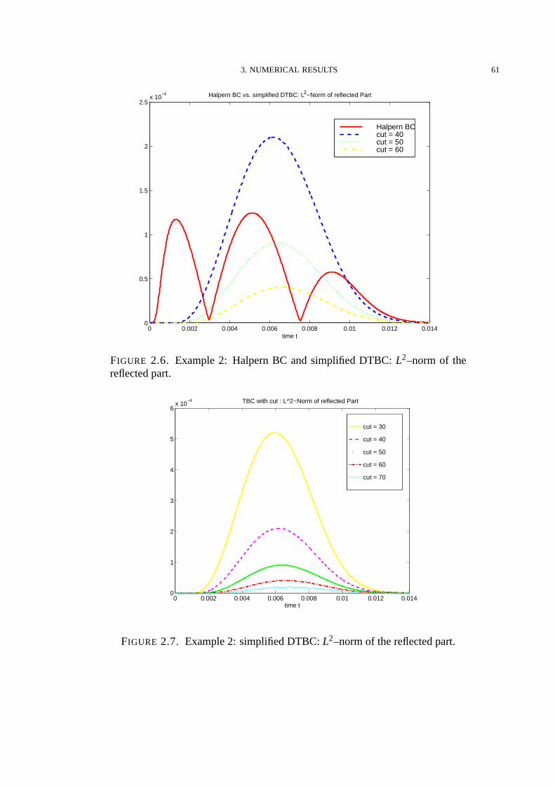
3. NUMERICAL RESULTS 61
0 0.002 0.004 0.006 0.008 0.01 0.012 0.0140
0.5
1
1.5
2
2.5x 10
−4 Halpern BC vs. simplified DTBC: L2−Norm of reflected Part
time t
Halpern BCcut = 40cut = 50cut = 60
FIGURE 2.6. Example2: HalpernBC andsimplified DTBC: L2–normof thereflectedpart.
cut = 30
cut = 40
cut = 50
cut = 60
cut = 70
0 0.002 0.004 0.006 0.008 0.01 0.012 0.0140
1
2
3
4
5
6x 10
−4
time t
TBC with cut : L^2−Norm of reflected Part
FIGURE 2.7. Example2: simplifiedDTBC: L2–normof thereflectedpart.
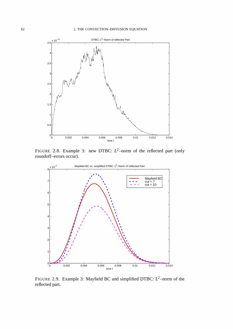
62 2. THE CONVECTION–DIFFUSIONEQUATION
0 0.002 0.004 0.006 0.008 0.01 0.012 0.0140
0.5
1
1.5
2
2.5
3
3.5
4
4.5x 10
−16 DTBC: L2−Norm of reflected Part
time t
FIGURE 2.8. Example3: new DTBC: L2–norm of the reflectedpart (onlyroundoff–errorsoccur).
0 0.002 0.004 0.006 0.008 0.01 0.012 0.0140
1
2
3
4
5
6
7
8x 10
−3 Mayfield BC vs. simplified DTBC: L2−Norm of reflected Part
time t
Mayfield BCcut = 7cut = 10
FIGURE 2.9. Example3: Mayfield BC andsimplifiedDTBC: L2–normof thereflectedpart.
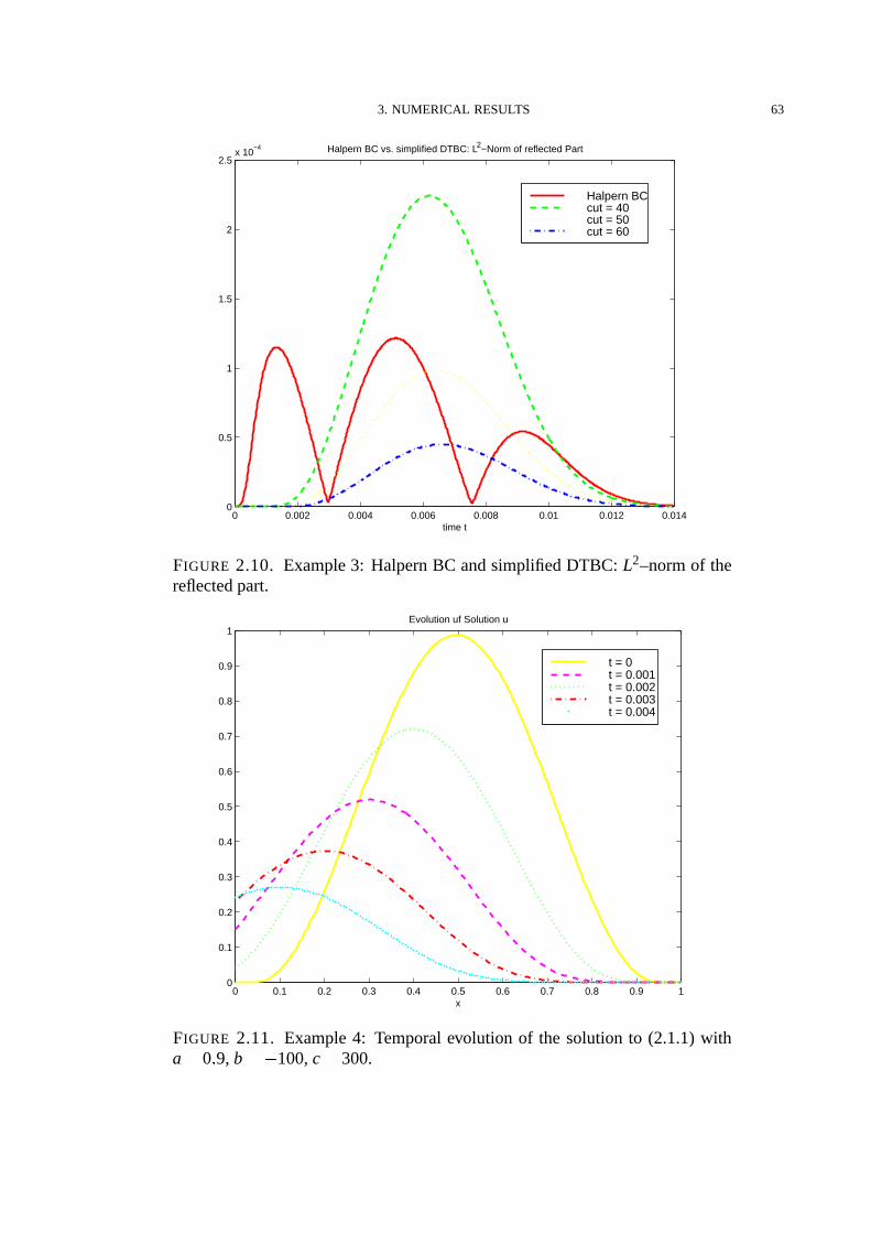
3. NUMERICAL RESULTS 63
0 0.002 0.004 0.006 0.008 0.01 0.012 0.0140
0.5
1
1.5
2
2.5x 10
−4 Halpern BC vs. simplified DTBC: L2−Norm of reflected Part
time t
Halpern BCcut = 40cut = 50cut = 60
FIGURE 2.10. Example3: HalpernBC andsimplifiedDTBC: L2–normof thereflectedpart.
0 0.1 0.2 0.3 0.4 0.5 0.6 0.7 0.8 0.9 10
0.1
0.2
0.3
0.4
0.5
0.6
0.7
0.8
0.9
1Evolution uf Solution u
x
t = 0t = 0.001t = 0.002t = 0.003t = 0.004
FIGURE 2.11. Example4: Temporalevolution of the solutionto (2.1.1)witha W 0Z 9, b WYX 100,c W 300.

64 2. THE CONVECTION–DIFFUSIONEQUATION
0 0.002 0.004 0.006 0.008 0.01 0.012 0.0140
0.2
0.4
0.6
0.8
1
1.2
1.4x 10
−16 DTBC: L2−Norm of reflected Part
time t
FIGURE 2.12. Example4: new DTBC: L2–norm of the reflectedpart (onlyroundoff–errorsoccur).
0 0.002 0.004 0.006 0.008 0.01 0.012 0.0140
0.5
1
1.5
2
2.5
3x 10
−3
time t
Mayfield BC vs. simplified DTBC: L2−Norm of reflected Part
Mayfield BCcut = 7cut = 10
FIGURE 2.13. Example4: Mayfield BC andsimplifiedDTBC: L2–normof thereflectedpart.
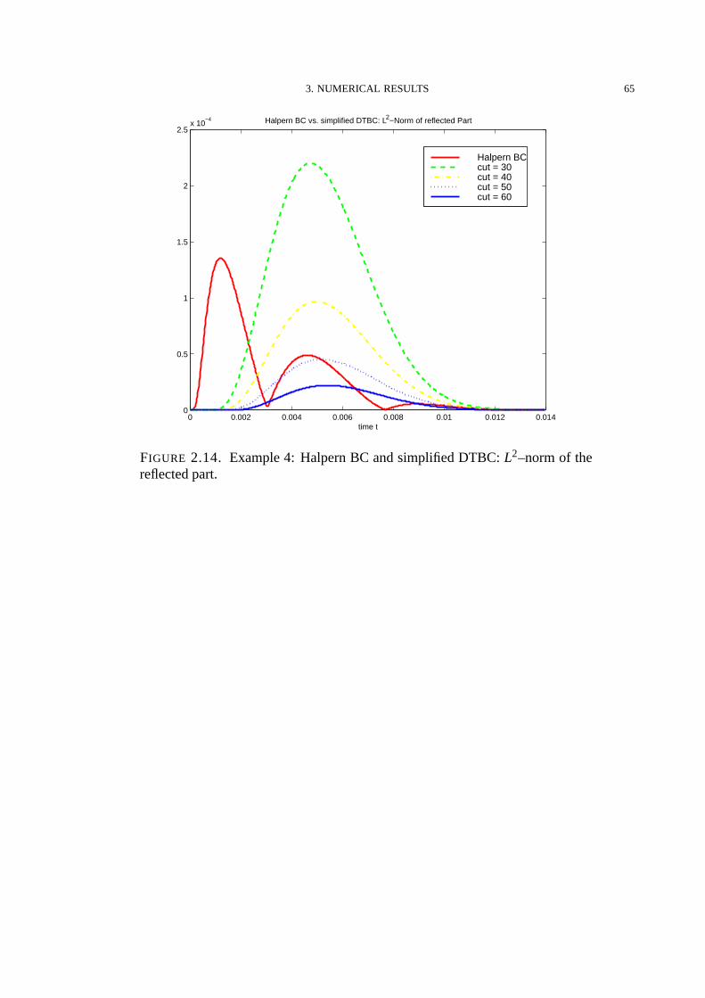
3. NUMERICAL RESULTS 65
0 0.002 0.004 0.006 0.008 0.01 0.012 0.0140
0.5
1
1.5
2
2.5x 10
−4 Halpern BC vs. simplified DTBC: L2−Norm of reflected Part
time t
Halpern BCcut = 30cut = 40cut = 50cut = 60
FIGURE 2.14. Example4: HalpernBC andsimplifiedDTBC: L2–normof thereflectedpart.

66 2. THE CONVECTION–DIFFUSIONEQUATION

CHAPTER 3
The Wide–AngleEquation of Underwater Acoustics
This Chapteris concernedwith a finite differencediscretizationof so–calledwide–angle“par abolic” equations(WAPEs).Thesemodelsappearasone–way wave propagationapprox-imationsto the Helmholtz equationin cylindrical coordinateswith azimuthalsymmetryandincludeasa specialcasetheSchrodingerequation.In particularwe will discussthediscretiza-tion of transparentboundaryconditionsusingtheideasof Chapter1.
In the past two decades“par abolic” equation(PE) modelshave beenwidely usedforwavepropagationproblemsin variousapplicationareas,e.g.seismology[U4], [U5], opticsandplasmaphysics(cf. thereferencesin [U3]). Furtherapplicationsto wavepropagationproblemscanbefound in radio frequency technology[U21]. Herewe will bemainly interestedin theirapplicationto underwateracoustics,wherePEshave beenintroducedby Tappert[U22]. Anaccounton thevastrecentliteratureis givenin thesurvey article[U18] andin thebook[U16].
1. Intr oduction to Underwater Acoustics
Onestandardtaskin oceanographyis to calculatetheunderwateracousticpressure p [ z\ r ]emergingfrom atime–harmonicpointsourcelocatedin thewaterat [ zs\ 0] . Here,r ^ 0 denotestheradial rangevariableand0 _ z _ zb thedepthvariable.Thewatersurfaceis at z W 0, andthe seabottomat z W zb. In our numericaltestsof discretetransparentboundaryconditions(in Section6) we will only dealwith horizontalbottoms(for thetreatmentof a slopingbottomsee[T21]). However, irregular bottom surfacesand sub–bottomlayerscan be includedbysimply extendingthe rangeof z. We denotethe local soundspeedby c [ z\ r ] , the densitybyρ [ z\ r ] , andthe attenuationby α [ z\ r ]a` 0. n [ z\ r ]bW c0 c c [ z\ r ] is the refractive index, with areferencesoundspeedc0 (usuallythesmallestsoundspeedin themodel). Thenthe referencewavenumberis k0 W 2π f c c0, where f denotesthe(usuallylow) frequencyof theemittedsound.Thesituationis shown in Figure3.1.
ThepressuresatisfiestheHelmholtzequation
1r
∂∂r
r∂p∂r
d ρ∂∂z
ρ e 1 ∂p∂z
dk2
0 N2p W 0\ r ^ 0\(3.1.1)
with thecomplex refractiveindex
N [ z\ r ]W n [ z\ r ] d iα [ z\ r ] c k0 Z(3.1.2)
In thefar field approximation(k0r f 1) the(complex valued)outgoingacousticfield
ψ [ z\ r ]W k0r p [ z\ r ] ee ik0r(3.1.3)
satisfiestheone–waywaveequation:
ψr W ik0 g 1 X L X 1 ψ \ r ^ 0Z(3.1.4)
67
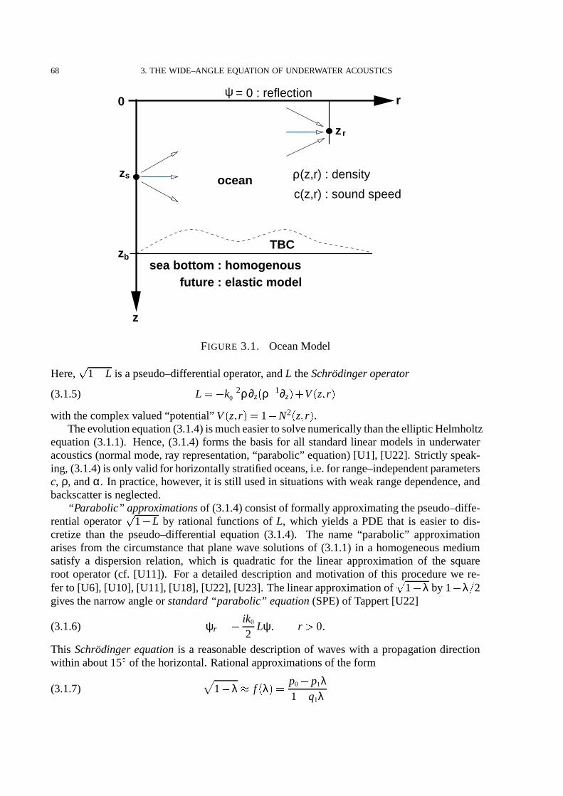
68 3. THE WIDE–ANGLE EQUATION OF UNDERWATER ACOUSTICS
= 0 : reflection0
ρ (z,r) : density
c(z,r) : sound speed
r
z
TBC
z
future : elastic model
s
zb
z r
ocean
sea bottom : homogenous
ψ
FIGURE 3.1. OceanModel
Here, g 1 X L is apseudo–differentialoperator, andL theSchrodinger operator
L WYX k e 20 ρ∂z [ ρ e 1∂z] d V [ z\ r ](3.1.5)
with thecomplex valued“potential” V [ z\ r ]W 1 X N2 [ z\ r ] .Theevolutionequation(3.1.4)is mucheasierto solvenumericallythantheelliptic Helmholtz
equation(3.1.1). Hence,(3.1.4) forms the basisfor all standardlinear modelsin underwateracoustics(normalmode,ray representation,“parabolic” equation)[U1], [U22]. Strictly speak-ing, (3.1.4)is only valid for horizontallystratifiedoceans,i.e.for range–independentparametersc, ρ, andα. In practice,however, it is still usedin situationswith weakrangedependence,andbackscatteris neglected.
“Parabolic” approximationsof (3.1.4)consistof formally approximatingthepseudo–diffe-rential operatorg 1 X L by rational functionsof L, which yields a PDE that is easierto dis-cretize than the pseudo–differential equation(3.1.4). The name“parabolic” approximationarisesfrom the circumstancethat planewave solutionsof (3.1.1) in a homogeneousmediumsatisfy a dispersionrelation, which is quadraticfor the linear approximationof the squareroot operator(cf. [U11]). For a detaileddescriptionandmotivation of this procedurewe re-fer to [U6], [U10], [U11], [U18], [U22], [U23]. Thelinearapproximationof g 1 X λ by 1 X λ c 2givesthenarrow angleor standard “par abolic” equation(SPE)of Tappert[U22]
ψr WhX ik0
2Lψ \ r ^ 0Z(3.1.6)
This Schrodinger equationis a reasonabledescriptionof waveswith a propagationdirectionwithin about15i of thehorizontal.Rationalapproximationsof theform
1 X λ j f [ λ ]W p0 X p1λ1 X q1λ
(3.1.7)

1. INTRODUCTION TO UNDERWATER ACOUSTICS 69
with real p0, p1, q1 yield thewide–angle“par abolic” equations(WAPE)
ψr W ik0
p0 X p1L1 X q1L
X 1 ψ \ r ^ 0Z(3.1.8)
In thesequelwe will repeatedlyrequirethat theslopeof theapproximatingfunction f shouldbenegative:
f k [ 0]W p0q1 X p1 _ 0Z(3.1.9)
Figure3.2illustratesthatthecondition(3.1.9)is quitenatural.With thechoicep0 W 1, p1 W 3c 4,
−0.2 0 0.2 0.4 0.6 0.8 1 1.20
0.2
0.4
0.6
0.8
1
1.2Approximation of Square Root Operator
λ
(1−λ)1/2
SPE: 1 − λ/2WAPE: (1 − 3λ/4)/(1 − λ/4)
FIGURE 3.2. Approximation f [ λ ] of thesquareroot g 1 X λ
q1 W 1c 4 ((1,1)–Pade approximantof g 1 X λ) oneobtainsthe WAPE of Claerbout [U4]. In[U11] Greenedeterminesthesecoefficientsby minimizing theapproximationerrorof g 1 X λover suitableλ–intervals. TheseWAPE modelsfurnisha muchbetterdescriptionof thewavepropagationup to anglesof about40i . To theauthor’s knowledge,no estimateof theapproxi-mationerrorfor suchparabolic/ wide–angle“parabolic” approximationexistsin theliterature.Also,higherorderanaloguesof (3.1.7),(3.1.8)[U8], [U13] andsplit–stepPadealgorithms[U9]havebeensuccessfullyusedfor acousticproblems.While wewill restrictourselveshereto theWAPE(3.1.8),weremarkthattheconstructionof discretetransparentboundaryconditions(seeSection5) couldbegeneralizedto higherorderPEsandeven3D–problems.
In this Chapterwe shall focuson boundaryconditions(BC) for theWAPE (3.1.8). At thewatersurfaceoneusuallyemploys a Dirichlet (“pressurerelease”)BC: ψ [ z W 0\ r ]lW 0. At theseabottomthe wave propagationin waterhasto be coupledto the wave propagationin thesedimentsof thebottom. Thebottomwill bemodeledasthehomogeneoushalf–spaceregionz ^ zb with constantparameterscb, ρb, andαb. Throughoutmostof this Chapterwe will usea fluid model for the bottomby assumingthat (3.1.8)alsoholds for z ^ zb, possiblywith adifferentrationalapproximation(3.1.7)(subjectto thecouplingcondition(3.3.9)).

70 3. THE WIDE–ANGLE EQUATION OF UNDERWATER ACOUSTICS
REMARK 1.1. Now wewantto explainshortlywhy therationalapproximationsof theform(3.1.7)areespeciallyappropriatefor far–field simulations.
If weassumeV, ρ, ρ e 1 m L∞ [ IRn] thentheSchrodingeroperator
L WYX k e 20 ρ∂z [ ρ e 1∂z] d V [ z](3.1.10)
with a homogeneousDirichlet BC at z W 0 is self–adjointin L2 [ IRn ;ρ e 1dz] with the densedomainD [ L ]bW H1
0 [ IRn ]'o ϕ p ρ e 1ϕzm H1 [ IRn ] . Thereforewe have the following spectral
representationfor all ψI m L2 [ IRn ;ρ e 1dz] :ψI [ z]lW M
∑j q 1
a jϕ j [ z] d ∞
Vb
a [ λ ] ϕλ [ z] dλ \ z ^ 0\(3.1.11)
wheretheϕ j aretheeigenfunctionsof L correspondingto theeigenvaluesλ j andtheϕλ denotethegeneralizedeigenfunctionsof L to λ.
In applicationsof underwateracousticsthe soundspeedc [ z] is typically larger in the seabottom than in the water. ThereforeV [ z] forms a “potential well” in the water region 0 _z _ zb, which typically givesrise to boundstatesof L that representthepropagatingmodesof(3.1.4)and(3.1.8). All of thecorrespondingeigenvaluessatisfy0 _ λ j _ Vb W 1 X c2
0 c c2b _ 1,
if c0 W minzr 0c [ z] . This is illustratedin Figure3.3whereσc WtsVb \ ∞ ] denotesthecontinuousundσp WYu λ j p j W 1\ZZZv\ M wyxz[ 0\ Vb ] thediscretespectrum.
z
|V [ z]\ σ [ L ]
Vb
1
σp
σc
0Dirichlet
BC
zb
FIGURE 3.3. PotentialV [ z] andspectrumσ [ L ] of theSchrodingeroperator
Thenthesolutionat ranger ^ 0 for theone–waywaveequation(3.1.4)is simply
ψ [ z\ r ]W M
∑j q 1
a j eik0 g 1e λ j e 1~ rϕ j [ z] d ∞
Vb
a [ λ ] eik0 1e λ e 1~ rϕλ [ z] dλ Z(3.1.12)
For λ ^ 1 we have only “evanescentmodes”, i.e. exponentialdampingfor the generalizedmodesin σc [ L ]o[ 1\ ∞ ] . If weassumefor a functiona thatsuppa xhs a1 \ a2 xsVb \ 1 holdsthen
we obtainwith ϕλ [ z]W ei λz for theintegral in (3.1.12)
limr ∞
a2
a1
a [ λ ] eik0 1e λ e 1~ r ei λzdλ W 0\ [ pointwisein z]\(3.1.13)
which follows from theLemmaof Riemann–Lebesgue.Fromtheabovewe concludethatonlypropagatingmodescontribute in the far field both for g 1 X λ and rational approximations.

1. INTRODUCTION TO UNDERWATER ACOUSTICS 71
Thereforea goodapproximationfor λ j is importantfor the far field. Figure3.4 illustratesthesituationshowing theSchrodingermodes(λ 1) andtheparabolicmodes(λ ^ 1).
0 1 2 30
1
Vb
Approximation of Square Root Operator
λ
Schroed. modes
real
parabol. modes
imag.
| (1 − λ)1/2 |
σp
σc
traveling. modes↑
1 − λ / 2
(4 − 3 λ) / (4 − λ)
FIGURE 3.4. Approximation f [ λ ] of thesquareroot g 1 X λ
In practicalsimulationsoneis only interestedin theacousticfield ψ [ z\ r ] in thewater, i.e.for0 _ z _ zb. While thephysicalproblemis posedontheunboundedz–interval [ 0\ ∞ ] , onewishesto restrict the computationaldomainin the z–directionby introducingan artificial boundaryat or below the seabottom. This artificial BC shouldof coursechangethe modelas little aspossible.Until recently, the standardstrategy wasto introduceratherthick absorbinglayersbelow the seabottomand then to limit the z–rangeby againimposinga Dirichlet BC [U6],[U8], [U19], [U20], [U23]. With acarefullydesignedabsorptionprofileandlayerthicknessthisstrategy hasbeenvery successful.But without a comparisonto theexacthalf–spacesolutionitis hardto estimatehow muchanabsorbinglayermodifiestheoriginalproblem.Also,absorbinglayersincreasethe computationalcosts,for SPE–or WAPE–simulationstypically by a factoraround2 [U18], [U26]. However, in simulationswithout attenuation(“f alseabsorbinglayermethod”[U18], [U26]) or overanelasticseabottom[U8], muchthickerabsorbinglayershavebeenusedto ensureaccuracy and,respectively, numericalstability.
In [T18] and[T20] Papadakisderived impedanceBCsor transparentboundaryconditions(TBC) for the SPEandthe WAPE, which completelysolvesthe problemof restrictingthe z–domainwithout changingthe physicalmodel: complementingthe WAPE (3.1.8)with a TBCat zb allows to recover — on the finite computationaldomain [ 0\ zb] — the exact half–spacesolution on 0 _ z _ ∞. As the SPEis a Schrodingerequation,similar strategies have beendevelopedindependentlyfor quantummechanicalapplications[T1], [T6], [T12] (cf. Chapter1).
Towardsthe end of this introductionwe shall now turn to the main motivation. WhileTBCs fully solve the problemof cutting off the z–domainfor the analyticalequation,their
72 3. THE WIDE–ANGLE EQUATION OF UNDERWATER ACOUSTICS
numericaldiscretizationis far from trivial. Indeed,all availablediscretizationsarelessaccuratethan the discretizedhalf–spaceproblemand they renderthe overall numericalschemeonlyconditionallystable[T6], [T16], [T19], [T26]. Theobjectof this work is to constructdiscretetransparentboundaryconditions(DTBC) for a Crank–Nicolsonfinite differencediscretizationof the WAPE suchthat the overall schemeis unconditionallystableand as accurateas thediscretizedhalf–spaceproblem.
In the literaturedifferentWAPEs(or WAPE andthe standard“parabolic” equation)havebeencoupledin the water and the seabottom. We also analyzein Section3 underwhichconditionsthe resultinghybrid model is conservative for the acousticenergy (weightedL2–norm).
While weshallassumeauniformdiscretizationin ranger, theinteriordepthzdiscretization(i.e. in thewatercolumn)maybenonuniform,andweshalldiscussin Subsection5.5strategiesfor the‘bestexteriordiscretization’(i.e. in theseabottom).
This Chapteris organizedasfollows: In Section2 we review theTBCs for theWAPE. InSection3 wediscussthecouplingof theWAPEto theSPEandin Section4 wederive theTBCfor theelasticPE.In Section5 discreteTBCsarederivedandanalyzed.Their superiorityoverexistingdiscretizationsis illustratedonseveralbenchmarkproblemsin Section6.
2. Transparent Boundary Conditions
In this Sectionwe first discussthewell–posednessof theevolution problemfor theWAPE(in the non–dissipative caseα W 0). Thenwe presentthe matching conditionsat the water–bottominterfacewhich hasto be taken into accountwhenwe derive afterwardstheconserva-tion/decayof theL2–norm. Finally we shortly review the transparentboundaryconditionfortheSPEandsketchthederivationtheTBC for WAPE.
2.1. The Well–Posednessof the Evolution Problem for the WAPE. Herewe shall dis-cussthewell–posednessof theevolution problemfor theWAPE in thecritical non–dissipativecase, i.e. for α W 0:
ψr W ik0 f [ L ]UX 1 ψ \ z ^ 0\ r ^ 0\(3.2.1)
subjectto the homogeneousDirichlet BC ψ [ 0\ r ]bW 0, andwith the rationalfunction f givenin (3.1.7).For simplicity of theanalysiswe only considertherange–independentsituation,i.e.α W α [ z] , ρ W ρ [ z] , V W V [ z] .
THEOREM 3.1(well–posednessof theWAPE). We assumethat the refractive index n [ z] ,thedensityρ [ z]^ 0, andρ e 1 [ z] areboundedfor z ^ 0. Then,theWAPEhasa uniquesolutionfor all initial data in the weightedL2–spaceL2 [ IRn ;ρ e 1dz] if and only if the pole of f [ λ ] atλ W qe 1
1 is not aneigenvalueof theoperator L with DirichletBCsat z W 0.
PROOF. In Theorem3.1 we assumedthat V, ρ, ρ e 1 m L∞ [ IRn ] . Then, the Schrodingeroperator
L WYX k e 20 ρ∂z [ ρ e 1∂z] d V [ z](3.2.2)
with a homogeneousDirichlet BC at z W 0 is self–adjointin L2 [ IRn ;ρ e 1dz] with the densedomain
D [ L ]lW H10 [ IRn ]o ϕ p ρ e 1ϕz
m H1 [ IRn ] Z(3.2.3)
2. TRANSPARENT BOUNDARY CONDITIONS 73
Wenow considertheoperatorf [ L ]lW p0 e p1L1e q1L definedas
f [ L ]lW ∞
e ∞f [ λ ] dPλ \(3.2.4)
with dPλ denotingtheprojectionvaluedspectralmeasureof theoperatorL (cf. [M1], [M7]).Accordingto [M1, TheoremXII.2.6] thedomainof f [ L ] is densein L2 [ IRn ;ρ e 1dz] if andonlyif λ W qe 1
1 , thepoleof f [ λ ] , is not aneigenvalueof L. In this casef [ L ] is self–adjointand,byStone’s Theorem[M7], ik0 f [ L ] generatesa unitaryC0–groupon L2 [ IRn ;ρ e 1dz] , which yieldstheuniquesolutionto (3.2.1).
REMARK 2.1. If λ coincideswith aneigenvalueλ j of L, then(3.2.1)still admitsa uniquemild solutionfor all initial datain theorthogonalcomplementof ϕ j , theuniqueeigenfunctioncorrespondingto λ j . Theorem3.1 generalizesthe well–posednessanalysisfor theWAPE onfinite intervalsgivenin [U2]. There,however, λ caneasilylie in the(pureeigenvalue)spectrumof L, whatthenrestrictstheclassof admissibleinitial conditions.
As q1 is muchsmallerthan1 in all practicalsimulations(14 in theWAPEof Claerbout;also
cf. [U11]), λ usuallylies in sVb \ ∞ ] , thecontinuousspectrumof L. Theorem3.1thenguaranteestheuniquesolvability of theevolution equation(3.2.1)for any initial data.Let uscomparethesituationathand(i.e. theWAPEontheoriginalunboundedinterval — andlateralsotheWAPEwith a TBC) to theWAPE restrictedto thez–interval s 0\ zmax with a homogeneousRobinBCatzmaxasasimplemodelfor anabsorbinglayer: there,L hasapureeigenvaluespectrumwhichinhibits thesolvability of (3.2.1)in severalcasesof practicalrelevance[U2].
2.2. The Matching Conditions and the Conservation of the Acoustic Power. Now weturn to thematchingconditionsandlater theTBCsat thewater–bottominterface(z W zb). Asthe densityis typically discontinuousthere,onerequirescontinuity of the (acoustic)pressureandthenormalparticlevelocity:
ψ [ zb e \ r ]lW ψ [ zb n \ r ]\(3.2.5a)
ψz [ zb e \ r ]ρw
W ψz [ zb n \ r ]ρb
\(3.2.5b)
whereρw W ρ [ zb e \ r ] is the waterdensityjust above the bottomandρb denotesthe constantdensityof thebottom.
With thesematchingconditions(3.2.5)weshallnow deriveanestimatefor theL2–decayofsolutionsto the WAPE (3.1.8),z ^ 0. We assumeρ W ρ [ z] andapply the operator1 X q1L to(3.1.8):
(3.2.6) 1 X q1Vd
q1k e 20 ρ∂z [ ρ e 1∂z] ψr
W ik0 p0 X 1 X[ p1 X q1 ] V d [ p1 X q1 ] k e 20 ρ∂z [ ρ e 1∂z] ψ Z
74 3. THE WIDE–ANGLE EQUATION OF UNDERWATER ACOUSTICS
Multiplying (3.2.6)by ψρ e 1, integratingby partson 0 _ z _ zb, andtakingtherealpartgives
∂r
zb
0p ψ p 2ρ e 1dz
W 2 [ p1 X q1 ] k0
zb
0Im sV p ψ p 2 ρ e 1dz X k e 2
0 ρ e 1w Im s ψzψ p zq zb e
dq1
zb
0Re sV ∂r p ψ p 2 X 2Im sV Im s ψrψ ρ e 1dz
dk e 2
0 ∂r
zb
0p ψz p 2 ρ e 1dz X 2k e 2
0 ρ e 1w Re s ψzrψ p zq zb e Z
(3.2.7)
Analogously, multiplying (3.2.6)by ψrρ e 1, andtakingtheimaginarypartwe get
[ p0 X 1] ∂r
zb
0p ψ p 2 ρ e 1dz
WX 2q1k e 10
zb
0Im sV p ψr p 2ρ e 1dz
d2q1k e 3
0 ρ e 1w Im s ψzrψr p zq zb e
d [ p1 X q1 ] zb
0Re sV ∂r p ψ p 2 d
2Im sV Im s ψrψ ρ e 1dz
dk e 2
0 ∂r
zb
0p ψz p 2 ρ e 1dz X 2k e 2
0 ρ e 1w Im s ψzψr p zq zb e Z
(3.2.8)
After aneasyalgebraicmanipulationweobtainfrom (3.2.7), (3.2.8)
(3.2.9) ∂r
zb
0p ψ p 2 ρ e 1dz
WYX 2C1
zb
0α
c0
c∂rψ
2ρ e 1dz X C1k e 1
0 ρ e 1w Im ∂rψz∂rψ
zq zb e \with
C1 W 2 [ p1 X q1 ] 2
p1 X p0q1
\ ∂r W Id iq1
p1 X q1
k e 10 ∂r Z
In thesamewayasimilarequationcanbederivedfor thebottomregionz ^ zb:
(3.2.10) ∂r
∞
zb
p ψ p 2 ρ e 1dz
WX 2C1αbc0
cb
∞
zb
∂rψ2
ρ e 1dzd
C1k e 10 ρ e 1
b Im ∂rψz∂rψzq zb n Z
Adding thetwo aboveequationswith (3.2.5)gives
∂r ψ [ Z\ r ] 2 WhX 2C1
∞
0α
c0
c∂rψ
2ρ e 1dz(3.2.11)
for theweightedL2–norm
ψ [ Z\ r ] 2 W ∞
0p ψ [ z\ r ](p 2 ρ e 1 [ z] dzZ(3.2.12)
In thedissipation–freecase(α 0) ψ [SZ\ r ] is conservedandfor α ^ 0 and p0q1 X p1 _ 0 itdecays.Thediscreteanalogueof this “energy”–conservation(or –decayfor α ^ 0) will bethemainingredientfor showing unconditionalstabilityof thefinite differenceschemein Section5.

2. TRANSPARENT BOUNDARY CONDITIONS 75
REMARK 2.2(L2–estimatefor SPE). For p1 W 1c 2, q1 W 0, (3.2.9)simplifiesto:
∂r
zb
0p ψ p 2 ρ e 1dz WhX 2
zb
0α
c0
cp ψ p 2 ρ e 1dz X 1
k0ρwIm s ψzψ p zq zb e Z(3.2.13)
2.3. The Transparent Boundary Condition for the SPEand WAPE. Now we shall re-view the transparentbottomboundaryconditionfor the SPEandsketchthe derivation of theTBC for theWAPE.We assumethattheinitial dataψI W ψ [ z\ 0] , which modelsa point sourcelocatedat [ zs\ 0] , is supportedin the interior domain0 _ z _ zb (otherwise,if the sourceiscloseto thebottomtheapproachof Section3 in Chapter1 canbeapplied).Also, let thebottomregion behomogeneous, i.e. let all physicalparametersbeconstantfor z ^ zb. Thebasicideaof thederivation is to explicitly solve theequationin thebottomregion, which is theexteriorof thecomputationaldomain [ 0\ zb ] . TheTBCfor theSPE(or Schrodingerequation)(1.1.10)readsnow:
ψ [ zb \ r ]WYX 1
g 2πk0
ei π4
ρb
ρw
r
0
ψz [ zb \ r X τ ] eibτ
g τdτ \(3.2.14)
with b W k0 [ N2b X 1] c 2. ThisBC is nonlocalin therangevariabler andinvolvesamildly singular
convolutionkernel.Equivalently, it canbewritten as
ψz [ zb \ r ]WYX 2k0
πee iπ
4 eibr ρw
ρb
ddr
r
0
ψ [ zb \ τ ] ee ibτ
g r X τdτ \(3.2.15)
andther.h.s.canbeexpressedformally asa fractional(12) derivative[T1], [T6], [T7]:
ψz [ zb \ r ]lWhX 2k0ee π4 i eibr ρw
ρb∂r ψ [ zb \ r ] ee ibr Z(3.2.16)
In [T7] thissquarerootoperatoris approximatedby rationalfunctionswhichleadsto ahierarchyof highly absorbing(but not any moreperfectlytransparent)BCsfor theSPE.By introducingauxiliary boundaryvariablestheseBCscanbeexpressedthroughlocal–in–r operators.Hence,thisallowsfor a “local” (2–level in r) discretizationscheme[T9]. Thisscheme,however, intro-ducesnumericalreflectionsat theartificial boundary, whoseamplitudedependson thechosenapproximationorderof theabovesquareroot operator.
In orderto derive theTBCfor theWAPEweconsider(3.2.6)in thebottomregion:
[ δbd
q1k e 20 ∂2
z ] ψr W i υbd [ p1 X q1 ] k e 1
0 ∂2z ψ \ z ^ zb \(3.2.17)
with
δb W 1 X q1 [ 1 X N2b ]\ υb W k0 p0 X 1 X[ p1 X q1 ]B[ 1 X N2
b ] ZAfter aLaplacetransformationof (3.2.17)in r weget
q1s X i [ p1 X q1 ] k0 ψzz[ z\ s]W k20 [ iυb X δbs] ψ [ z\ s]Z(3.2.18)
Sinceits solutionhasto decayasz ∞ weobtain
ψ [ z\ s]'W ψ [ zb n \ s] exp X k0 iυb X δbsq1s X i [ p1 X q1 ] k0
[ z X zb] \ z ^ zb \(3.2.19)
andwith thematchingconditions(3.2.5)this gives
ψz [ zb e \ s]WYX k0
ρw
ρb iυb X δbs
q1s X i [ p1 X q1 ] k0
ψ [ zb e \ s]Z(3.2.20)
76 3. THE WIDE–ANGLE EQUATION OF UNDERWATER ACOUSTICS
Here,again g denotesthebranchof thesquareroot with a nonnegative realpart. An inverseLaplacetransformation[S2] yieldstheTBCat thebottomfor theWAPE:
(3.2.21) ψ [ zb \ r ]WX iηρb
ρwψz [ zb \ r ]
d βηρb
ρw
r
0ψz [ zb \ r X τ ] eiθτeiβτ J0 [ βτ ] d iJ1 [ βτ ] dτ \
η W 1k0
q1
δb\ β WhX p1 X p0q1
2q1
k0
δb\ θ W p1 X q1
q1
k0 \whereJ0, J1 denotetheBesselfunctionsof order0 and1, respectively. This is a slight gener-alizationof the TBC derived in [T20] wherep0 wasequalto 1. Equivalently, (3.2.21)canbewritten as
(3.2.22) ψz [ zb \ r ]lW iη e 1ρw
ρbψ [ zb \ r ]
d βη e 1ρw
ρb
r
0ψ [ zb \ r X τ ] eiθτeiβτ J0 [ βτ ]UX iJ1 [ βτ ] dτ Z
BothTBCsarenonlocalin r; in rangemarchingalgorithmsthey thusrequirestoringthebottomboundarydataof all previousrangelevels.
Weremarkthattheasymptoticbehaviour(for r ∞) of theconvolutionkernelin theTBC(3.2.15)is O r e 3 2 , which canbe seenafter an integrationby parts. Using the asymptoticbehaviour of theBesselfunctions(see(3.5.5)) onefindsthattheconvolution kernelof (3.2.22)alsodecayslikeO r e 3 2 .
3. Coupled Models for Underwater Acoustics
We shall now briefly commenton coupledmodelsfor underwateracoustics,asproposedin [T19], [T20]. In [T20] theWAPEfor theocean[ 0 _ z _ zb ] is coupledto theSPEfor theseabottom [ z ^ zb ] . In fact,thesemodelsarecoupledvia aTBC correspondingto theSPE,but thisis equivalentto thehalf–spaceproblem.Herewewantto pointoutamathematicalambiguityofthis couplingthatmay stronglyinfluencethenumericalstability of thediscretizationscheme.To this endwe discussthis coupledWAPE–SPEmodel in the simplecaseof constantsoundspeedc anddensityρ, which is ratherunrealistic,but it illustratesthesituation.
3.1. The coupled WAPE–SPE model. Let us first review the WAPE (3.2.1) with theSchrodingeroperatorL WX k e 2
0 ∂2z. Whendiscretizing(3.2.1)oneusuallyappliesthe opera-
tor 1 X q1L to (3.2.1)which givesthefollowing PDEof “Sobolev type” [M6]
[ 1 X q1L ψr W ik0 p0 X 1 X[ p1 X q1 ] L ψ \ z ^ 0\ r ^ 0Z(3.3.1)
Since the operatorsin the numeratorand denominatorof (3.1.8) commute(even for non–constantc and ρ) this stepis mathematicallyrigorous,and (3.3.1) is easyto discretize(seeSection5).
Disregardingfor the momentthenonlocalityof the involvedpseudo–differentialoperator,onewould formally want to write the evolution equationfor the coupledmodel (WAPE andSPE)as
ψr W ik0Aψ(3.3.2)

3. COUPLEDMODELS FOR UNDERWATER ACOUSTICS 77
with
(3.3.3a)
Aψ Wp0
dp1k e 2
0 ∂2z
1d
q1k e 20 ∂2
z
X 1 ψ \ 0 _ z _ zb \
k e 20
2∂2
zψ \ z ^ zb Z(3.3.3b)
However, theright handsideof (3.3.2)is notwell–defined,dueto thenonlocalityof thepseudo–differentialoperatorin (3.3.3a).Also, its reformulationasin (3.3.1)is not any longerjustifiedin thecoupledcase.Evenin thedissipation–freecaseit wouldresultin anon–conservativeevo-lution equationandhencein a non–conservative numericalscheme(neverthelessthis strategyis usedin [T20]). This is illustratedin Example3 of Section6.
Usingmoreinvolvedpseudo–differentialoperatorswe will find a correctandconservativeinterpretationof (3.3.2),(3.3.3). Wefirst considerthepseudo–differentialoperatorf [ L ] appear-ing in theWAPE(3.2.1)with L WYX k e 2
0 ∂2z. Dueto theBC at z W 0 it canbeexpressedin terms
of Fourier–sinetransformsas
f [ L ] ψ [ z]W 2π
∞
0
∞
0Φ [ ξ ] ψ [ y] sin[ ξy] sin[ ξz] dydξ \(3.3.4)
with thesymbol
Φ [ ξ ]W p0 X p1k e 20 ξ2
1 X q1k e 20 ξ2
Z(3.3.5)
In thecoupledWAPE–SPEmodelonewould formally wantto write theevolutionequationas(3.3.2),(3.3.3). However, asthepseudo–differentialoperatorin (3.3.3a)is nonlocal,actingon L2 [ IRn] , it cannotbesimply restrictedto theinterval 0 _ z _ zb. It is thereforeappropriateto definethe coupledevolution equationon the symbol level of the two involved operators(cf. [U10], [M4]). Without attenuationboth the SPEand the WAPE conserve the L2–normandthediscreteanalogueof this conservationis themainingredientfor showing unconditionalstability of thefinite differenceschemein Section5. Thereforewe postulatethat thecoupledmodelalsohasto conserve the L2–norm. This canbe achieved if the operatorA on the righthandsideof (3.3.2)is interpretedastheWeyl operator (see[U10])
Aψ [ z]W 2π
∞
0
∞
0a
yd
z2
\ ξ ψ [ y] sin[ ξy] sin[ ξz] dydz(3.3.6)
to thesymbol
a [ z\ ξ ]W Φ [ ξ ]UX 1\ 0 _ z _ zb \X k 2
02 ξ2 \ z ^ zb Z(3.3.7)
As a [ z\ ξ ] is real,onereadilyverifiesthat theevolution equation(3.3.2),(3.3.6)conservestheL2–norm.
Due to the pole of the symbolΦ [ ξ ] it would be quite difficult to appropriatelydiscretize(3.3.2), (3.3.6),andit is beyond our scopehere. We remarkthat finite differenceschemesofpseudo–differentialequationswith smoothsymbolshaverecentlybeenstudiedin [F4].

78 3. THE WIDE–ANGLE EQUATION OF UNDERWATER ACOUSTICS
However, its discretizationusingthe ideasof Markowich andPoupaud[F5] would beverydifficult andwill bea topicof futureresearch.
3.2. The coupling of different WAPEs. Fromtheabove we concludethat it is not advis-able to couplethe WAPE andthe SPEnumerically. As an alternative we shall now analyzecouplingsof WAPEswith differentparametersp0, p1, q1 that canbe reformulatedasa PDE,like in (3.3.1).Thecoupledmodel
ψr W ik0
p0 [ z]UX p1 [ z] L1 X q1 [ z] L X 1 ψ(3.3.8)
is well–definedandcanbe transformedto (3.3.1)if thenumeratoranddenominatorin (3.3.8)commute.Underthecondition
p1 [ z] c q1 [ z]W : µ W const(3.3.9)
we canrewrite thepseudo–differentialoperatorin (3.3.8)as
p0 [ z]UX p1 [ z] L1 X q1 [ z] L W µ τ [ z]UX µe 2σ [ z] L X 1
τ [ z]X µe 2σ [ z] L \(3.3.10)
with
τ [ z]W µ X p0 [ z] e 1 \ σ [ z]W p21 [ z] p1 [ z]UX p0 [ z] q1 [ z] e 1 Z(3.3.11)
Herethe numeratoranddenominatorcommute,andhence(3.3.8)canbe written in the formof (3.3.1). Theresultingevolution equationis conservative in L2 [ IRn ; [ σρ ] e 1dz] andit allowsfor a conservative andunconditionallystablediscretization(seeSection5 andExample3 inSection6).
If theparametersp0, p1, q1 arefixedin onemedium,condition(3.3.9)still leavestwo freeparametersto chooseadifferentrationalapproximationmodelof g 1 X λ for thesecondmedium(cp. [U11]). Hence,onecanin factobtaina betterapproximationin thesecondmediumthanwith theoriginally intended“parabolicapproximation”.
4. The Transparent Boundary Condition for an Elastic Bottom
In [T3] wepresentedthefollowing smallremarkon thecouplingof theSPEwith anelastic“par abolic” equation(EPE)for theseabottom[U7], [U12], [U24]. In [T19], [T20] a TBC forthis couplingwasderived.It readsfor theLaplacetransformedwavefield:
(3.4.1) ψ [ zb \ s]lWhX ρb
ρw
1k0N4
s
1
Mp [ s]
2Ms [ s] d N2s
2 X 4 Mp [ s] Ms [ s] Ms [ s] d N2s ψz [ zb \ s]\
with thenotation
Mp [ s]W 1 X N2p X i
2k0
s\ Ms [ s]W 1 X N2s X i
2k0
sZ(3.4.2)
Here, Np W npd
iαp c k0 and Ns W nsd
iαsc k0 denotethe complex refractive indicesfor thecompressionalandshearwavesin thebottom. In a tediouscalculationthis BC canindeedbeinverseLaplacetransformed(using[S2]) andit reads:
ψ [ zb \ r ]lW Cr
0ψz [ zb \ r X τ ] eiωτg [ τ ] dτ X 2iϕ
r
0ψzr [ zb \ r X τ ] eiωττ e 1
2 dτ \(3.4.3)
4. THE TRANSPARENT BOUNDARY CONDITION FOR AN ELASTIC BOTTOM 79
with
C WYX ρb
ρw
2
k5 20 N4
s
2π
eπ4 i \ ω W k0
2N2
p X 1 \ ϕ WhX k0
2N2
p X N2s \
g [ τ ]WhX 3 1 X eiϕτ τ e 52d
ik0
23N2
p X N2s X 2N2
s eiϕτ τ e 32
d k20
2N4
p X N2pN2
sd 1
2N4sd
N2p X N2
s τ e 12 W O τ e 1
2 ZWhile this inversetransformationwascarriedout numericallyin [T17], [T19], [T20], our an-alytical TBC maysimplify thediscretizationof this coupledmodel. However, a discretizationof theTBC for a numericalimplementationis possiblebut againstthespirit of our approachtoderive theBCsonadiscretelevel. Also thestabilityof theresultingschemeis unclear. DTBCsfor theSPE–EPEcoupling(in thespirit of Section5) arenot derivedyet, mainly sincewe donothavea conservativeformulationof thecoupledelastic–fluidPE.
Note that the TBC (3.4.3) for the elasticPE hasthe sameform as the TBC for the SPE(3.2.14)but thesingularityin theintegral kernelis stronger(of order3c 2).
DERIVATION (of (3.4.3)). With theabbreviation ψ [ s] : W ψ [ zb \ s] andthenotation
mp [ s]W k0
2Mp [ s]WYX i s s X i
k0
2[ N2
p X 1] \(3.4.4a)
ms [ s]W k0
2Ms [ s]WYX i s s X i
k0
2[ N2
s X 1] \(3.4.4b)
(3.4.1)reads
ψ [ s]WYX ρb
ρw
1k0N4
s
k0
2
4k0
ms [ s] d N2s
2
mp [ s] X 42k0
ms [ s] 2k0
ms [ s] d N2s ψz [ s]
WYX ρb
ρw
8g 2
k5 20 N4
s
ms [ s] d k04 N2
s2
mp [ s] X 4 ms [ s] ms [ s] d k0
2N2
s ψz [ s]\(3.4.5)
wherewedenotethecontentof thesquarebracketsby f [ s X σ ] with
σ W ik0
2[ N2
p X 1]Z(3.4.6)
Weobserve thatwe canwrite
mp [ s]WYX i s s X σ \ ms [ s]WX i s s X σ dik0
2[ N2
p X N2s ] Z(3.4.7)
Thenext stepis ashift in theargumentof ψz [ s] in (3.4.5)by σ:
ψ [ zb \ s d σ ]WYX ρb
ρw
8g 2
k5 20 N4
s
f [ s] ψz [ zb \ s d σ ]\(3.4.8)

80 3. THE WIDE–ANGLE EQUATION OF UNDERWATER ACOUSTICS
With g X i W ee π4 i weobtainfor f [ s]f [ s]lW X is
d k02 [ N2
p X N2s ] d k0
4 N2s
2
ee π4 i g s
X ee π4 i s
dik0
2[ N2
p X N2s ]B[ X i ] s
dik0
2[ N2
p X N2s ]=s s d
ik0
2N2
p \(3.4.9)
where
s? 2 WYXs s dik0
2N2
p X ik0
4N2
s 2WYXs s d
ik0
2[ N2
p X N2s ] s s d
ik0
2N2
p d k20
16N4
s \(3.4.10)
f [ s]lW eπ4 i 1
g sk2
0
16N4
s X sd
ik0
2[ N2
p X N2s ] s
dik0
2N2
p
d sd
ik0
2[ N2
p X N2s ]s s d
ik0
2N2
p W e
π4 i s
dik0
2[ N2
p X N2s ]UX g s X i
k0
2[ N2
p X N2s ] 1
g s
sd
ik0
2N2
pd k2
0
16N4
s1
g s
W eπ4 i g s X γ X g s
d γ1
g ssd
ik0
2N2
pd k2
0
16N4
s1
g s\
(3.4.11)
with
γ WX ik0
2[ N2
p X N2s ]Z(3.4.12)
Now thetransformedtransparentboundaryconditionreads
ψ [ s d σ ]W C ik0
2N2
p g s X γ X g sd γ
1
g sd k2
0
16N4
s1
g sψz [ s d σ ]
dC g s X γ X g s
d γ1
g su sψz [ s d σ ]w\
(3.4.13)
with theconstant
C WhX ρb
ρw
8g 2
k5 20 N4
s
eπ4 i Z(3.4.14)
An inverseLaplacetransformationof (3.4.13)using(IL.6), (IL.7) yields
ψ [ r ] ee σr W Cr
0ψz [ r X τ ] ee σ r e τ ~ g1 [ τ ] dτ
dC
r
0X ∂
∂τψz [ r X τ ] ee σ r e τ ~ g2 [ τ ] dτ \(3.4.15)

4. THE TRANSPARENT BOUNDARY CONDITION FOR AN ELASTIC BOTTOM 81
wherewecomputewith thehelpof (IL.4), (IL.5)
g1 [ τ ]We 1 ik0
2N2
p g s X γ X g sd γ
1
g sd k2
0
16N4
s1
g s
W ik0
2N2
p e 1 g s X γ X g sd k2
0
4[ N2
p X 12N2
s ] 2e 1 1
g s
W ik0
4g πN2
p [ 1 X eγτ ] τ e 32d k2
0
4g π[ N2
p X 12N2
s ] 2 τ e 12 \
(3.4.16a)
g2 [ τ ]W e 1 g s X γ X g sd γ
1
g sW 1
2g π[ 1 X eγτ ] τ e 3
2d γ
g πτ e 1
2
W 12g π
[ 1 X eγτ ] τ e 32d γτ e 1
2
q g3 τ ~d γ
2g πτ e 1
2
q g4 τ ~\(3.4.16b)
I3 W r
0X ∂
∂τψz [ r X τ ] ee σ r e τ ~ g3 [ τ ] dτ
W r
0ψz [ r X τ ] ee σ r e τ ~ gk3 [ τ ] dτ X ψz [ r X τ ] ee σ r e τ ~ g3 [ τ ] τ q r
τ q 0
q 0 with ψz 0~q 0~Z(3.4.16c)
Thustheboundarycondition(3.4.15)readsnow
ψ [ r ] ee σr W Cr
0ψz [ r X τ ] ee σ r e τ ~ g1 [ τ ] d gk3 [ τ ] dτ
dC
r
0X ∂
∂rψz [ r X τ ] ee σ r e τ ~ g4 [ τ ] dτ
W Cr
0ψz [ r X τ ] ee σ r e τ ~ g1 [ τ ] d gk3 [ τ ] dτ
dC
r
0ψzr [ r X τ ] ee σ r e τ ~ X σψz [ r X τ ] ee σ r e τ ~ g4 [ τ ] dτ \
(3.4.17)
i.e.
ψ [ r ]lW Cr
0ψz [ r X τ ] eστg [ τ ] dτ d r
0ψzr [ r X τ ] eστg4 [ τ ] dτ \(3.4.18)
where
g [ τ ]W g1 [ τ ] d gk3 [ τ ]X σg4 [ τ ] Z(3.4.19)
Wecalculate
gk3 [ τ ]W 12g π
X 32[ 1 X eγτ ] τ e 5
2 X γeγτ τ e 32 X γ
2τ e 3
2
W 14g π
X 3 [ 1 X eγτ ] τ e 52 X 2γ [ 1
2d
eγτ ] τ e 32 \
(3.4.20a)
σg4 [ τ ]W σγ2g π
τ e 12 W 1
4g πk2
0
2[ N2
p X 1]B[ N2p X N2
s ] τ e 12 \(3.4.20b)
82 3. THE WIDE–ANGLE EQUATION OF UNDERWATER ACOUSTICS
andtherefore
g [ τ ]W 14g π
ik0N2p 1 X eγτ τ e 3
2d
k20 N2
p X 12N2
s2τ e 1
2 X 3 1 X eγτ τ e 52
dik0 N2
p X N2s
12d
eγτ τ e 32 X k2
0
2N2
p X 1 N2p X N2
s τ e 12
W 14g π
k20
2N4
p X N2pN2
sd 1
2N4sd
N2p X N2
s τ e 12
dik0
23N2
p X N2s X 2N2
s eγτ τ e 32 X 3 1 X eγτ τ e 5
2
W O [ τ e 12 ]\ τ 0Z
(3.4.21)
Finally, wedefineϕ, ω by γ W : iϕ, σ W : iω, andset
g [ τ ]W 4g πg [ τ ]\ C W C
4g π(3.4.22)
We remarkthat thewell–posednessof thecoupledanalyticproblemis not provenyet andwill bea topic of futureresearch.
5. DiscreteTransparent Boundary Conditions
In thisSectionweshalldiscusshow to discretizetheTBCs(3.2.14),(3.2.21)in conjunctionwith aCrank–Nicolsonfinite differenceschemefor theSPEandtheWAPE.Mostof thetimeweshallonly consideruniformgridsin z andr. While auniformrangediscretizationis crucialforourconstructionof discreteTBCs,thisconstructionis independentof the(possiblynonuniform)z–discretizationon theinteriordomain.
For simplicity we first considertheuniform grid zj W jh, rn W nk (h W ∆z, k W ∆r) andtheapproximationψn
j ψ [ zj \ rn] . ThediscretizedWAPE (3.2.6)thenreads:
(3.5.1) 1 X q1Vnn 1
2j
dq1k e 2
0 ρ jD0h2[ ρ e 1
j D0h2] Dk ψn
j
W ik0 p0 X 1 X[ p1 X q1 ] Vnn 12
jd [ p1 X q1 ] k e 2
0 ρ jD0h2[ ρ e 1
j D0h2] ψn
jd ψnn 1
j
2\
with Vnn 1
2j : W V [ zj \ rnn 1
2] andtheusualdifferenceoperators
Dk ψnj W ψnn 1
j X ψnj
k\ D0
h2ψn
j W ψnj n 1
2X ψn
j e 12
hZ
It is well known thatthisschemeis secondorderin h andk andunconditionallystable[U2].Proceedingsimilarly to thederivationof (1.2.6)onecanshow
Dk ∑j ZZ
ψnj
2
ρ jWYX C1k e 1
0 ∑j ZZ
Im Vnn 1
2j ψnn 1
2j
d iq1
p1 X q1
k e 10 Dk ψn
j
2
ρ e 1j \(3.5.2)
with C1 W 2 [ p1 X q1 ] 2 c [ p1 X p0q1 ] . Hence,thescheme(3.5.1)preservesthediscreteweightedL2–norm ψn 2
2 W h∑ j ZZ p ψnj p 2 c ρ j in thedissipation–freecase(V real). This alsoholdswhen
usingahomogeneousDirichlet BC at j W 0.

5. DISCRETETRANSPARENT BOUNDARY CONDITIONS 83
5.1. Discretization strategiesfor the TBC. In theliteraturethreedifferentstrategieshavebeenproposedto discretizeTBCs,mostly, however, just for theSchrodingerequation.Firstwereview (asin Chapter1) a known ad–hocdiscretizationof theanalyticTBC.
Discretized TBC of Thomson and Mayfield. In [T26] ThomsonandMayfield usedthefollowing discretizedTBC for theSPE:
ψnJ X ψn
J e 1 W h
2Bk12
ψnJ X Bk ne 1
∑mq 1
ψne mJ X ψne m
J e 1˜ m\(3.5.3)
with
B WhX [ 2πk0 ]Ae 12 e
π4 i ρb
ρw\ Bk¡W e
i2bk sin[ 1
2bk]12bk
\ ˜ m W eibmk
2 md 1
2
ZOn the fully discretelevel this BC is not perfectlytransparentany moreandit mayalsoyieldanunstablenumericalscheme.In analogyto theanalyticTBC (3.2.14)it requirestheboundarydatafrom thewhole“pastrange” s 0\ rne 1 .
To comparenumericallyour discreteTBC for theWAPE to thediscretizedTBC we useadiscretizationof theTBC (3.2.21)for theWAPEthatis analogousto (3.5.3):
r
0ψz [ zb \ rn X τ ] eiθτeiβτ J0 [ βτ ] d iJ1 [ βτ ] dτ
W ne 1
∑mq 0
rm 1
rm
ψz [ zb \ rn X τ ] eiθτ J0 [ βτ ] d iJ1 [ βτ ] dτ
j ne 1
∑mq 0
ψne mJ X ψne m
J e 1
hJ0 [ βrmn 1
2] d iJ1 [ βrmn 1
2] rm 1
rm
eiθτ dτ \with thedampedBesselfunctionsJν [ z] : W eizJν [ z] , z m IC. This yieldsthefollowing discretizedTBC:
ψnJ X ψn
J e 1 W ihη
ρw
ρbψn
J X Bk ne 1
∑mq 0
ψne mJ X ψne m
J e 1˜ m\(3.5.4)
with
Bk¢W iβei2θk sin[ 1
2θk]12θ
\ ˜ m W eiθmk J0 [ βrmn 12] d iJ1 [ βrmn 1
2] Z
REMARK 5.1. In far field simulationsonehasto evaluateJν [ z] for largecomplex z, whennumericallycalculatingtheseconvolution coefficients ˜ n. This, however, is a ratherdelicateproblem,andmany standardsoftwareroutinesarenotableto evaluateJν [ z] for largecomplex z.This is dueto theexponentialgrowth of theBesselfunctionsfor fixedν and p zp ∞ (see[S1]):
Jν [ z]W 2πz
12
cos z X νπ2
X π4
de£ Im z£ O p zp e 1 \ X π _ argz _ π Z(3.5.5)
For this reasonweusedasubroutineof Amos[C1] (seealso[C2], [C3]) to evaluatethedampedBesselfunctionsJν [ z] , Im z ` 0 (note that Im β ` 0 for the standardparameterchoicesin(3.1.7): p1 X p0q1 ^ 0 andq1 ^ 0).

84 3. THE WIDE–ANGLE EQUATION OF UNDERWATER ACOUSTICS
In [T16] Mayfield showed for the attenuation–freecasethat the discretizedTBC for theSPE(3.5.3)destroys theunconditionalstability of theunderlyingCrank–Nicolsonscheme(cf.Theorem1.2)andonecanexpecta similar behaviour for theWAPE.Theseexisting discretiza-tions alsoinducenumericalreflectionsat the boundary, particularlywhenusingcoarsegrids.Hence,theexisting discretizedTBC [T16], [T26] exhibits bothstability problemsandreducedaccuracy, which mayrequiretheusageof unnecessarilyfinegrids.
Semi–DiscreteTBC of Schmidt andDeuflhard. In thesemi–discreteapproachof SchmidtandDeuflhard[T23] a TBC is derivedfor thesemi–discretized(in r) SPE,which alsoappliesfor nonuniformr–discretizationsandrange–dependentcoefficientsin theexteriordomain.ThisTBC yields an unconditionallystablemethod(in conjunctionwith an interior finite elementscheme)[T24]. While thesemi–discreteapproachstill exhibits smallresidualreflectionsat theartificial boundary, thediscreteTBC is reflection–free[T24] (in Subsection5.5we shallreturnto thiscomparisonwhendiscussingthe‘bestexteriordiscretization’).In therecentarticle[T25]themethodsof [T24] areextendedto nonuniformr–discretizationsandrange–dependentpoten-tials.
DiscreteTBC. Insteadof usinganad–hocdiscretizationof theanalyticTBCslike (3.5.3)or (3.5.4)wewill constructdiscreteTBCsfor thefully discretizedhalf–spaceproblem,asdonein Chapter1. Our new strategy solvesboth problemsof the discretizedTBC at no additionalcomputationalcosts.With our DTBC thenumericalsolutionon thecomputationaldomain0 j J exactlyequalsthediscretehalf–spacesolution(on j m IN0) restrictedto thecomputationaldomain0 j J. Therefore,our overall schemeinherits the unconditionalstability of thehalf–spacesolutionthatis impliedby thediscreteL2–estimate(3.5.2).
5.2. Derivation of the DTBC. To derive theDTBC we will now mimic thederivationoftheanalyticTBCsfrom Section2 onadiscretelevel. For theinitial dataweassumeψ0
j W 0\ j `J X 2 andsolvethediscreteexteriorproblemin thebottomregion,i.e. theCrank–Nicolsonfinitedifferencescheme(3.5.1)for j ` J X 1:
Rδbd
q∆2h [ ψnn 1
j X ψnj ]lW i Rκb
d ∆2h [ ψnn 1
jd ψn
j ]\(3.5.6)
with
δb W 1 X q1 [ 1 X N2b ]\ R W 2k0
p1 X q1
h2
k\ q W k
2q1
p1 X q1
k e 10 \
κb W k2
k0 p0 X 1 X[ p1 X q1 ]B[ 1 X N2b ] \
where∆2hψn
j W ψnj n 1 X 2ψn
jd ψn
j e 1, andR is proportionalto theparabolicmeshratio. By usingthe ¤ –transform(for moredetailsseeAppendix):
¤yu ψnj w¥W ψ j [ z] : W ∞
∑nq 0
ψnj ze n \ z m IC\ p zp3^ 1\(3.5.7)
(3.5.6)is transformedto
zd
1d
iq [ z X 1] ∆2hψ j [ z]WhX iR δb [ z X 1]UX iκb [ z d
1] ψ j [ z]Z(3.5.8)

5. DISCRETETRANSPARENT BOUNDARY CONDITIONS 85
The solutionof the resultingsecondorder differenceequationtakes the form ψ j [ z]¦W ν j1 [ z] ,
j ` J X 1, whereν1 [ z] solves
ν2 X 2 1 X iR2
δb [ z X 1]X iκb [ z d1]
zd
1d
iq [ z X 1] ν d1 W 0Z(3.5.9)
For the decreasingmode(as j ∞) we require p ν1 [ z](p(_ 1. We obtain the ¤ –transformedDTBCas
ψJ e 1 [ z]W ν e 11 [ z] ψJ [ z]\(3.5.10)
andin a tediouscalculation(analogousto the onein Chapter1, page13) this canbe inversetransformedexplicitly:
CALCULATION (of [ 1 diq ]3¤ e 1 ν e 1
1 [ z] ). First wewrite [ 1 diq ] ν e 1
1 [ z] appropriately:
[ 1 diq ] ν e 1
1 [ z]W 1d
iq X iR2
δb [ z X 1]X iκb [ z d1]
zd 1e iq
1n iq
d X iR2
δb [ z X 1]X iκb [ z d1]
zd 1e iq
1n iq
2 [ 1 diq ]UX iR
2δb [ z X 1]UX iκb [ z d
1]zd 1e iq
1n iq
W 1d
iq X iR2
[ δb X iκb ] zzd
eiξd iR
2δb
diκb
zd
eiξ X iR2
1
zd
eiξ δb [ z X 1]UX iκb [ z d
1] δb X q4R
[ z X 1] d i4R
X κb [ z d1]
W 1d
iq X iR2
[ δb X iκb ] zzd
eiξd iR
2δb
diκb
zd
eiξ § iR2
g Az2 X 2Bzd
C
zd
eiξ \
(3.5.11)
with ξ W arg 1e iq1n iq andtheconstantsgivenby
A WI[ δb X iκb ] δb X iκbd
i4R
[ 1 diq ] \(3.5.12a)
B W δ2bd κ2
b X 4R
[ κbd δbq]\(3.5.12b)
C WI[ δbd
iκb ] δbd
iκb X i4R
[ 1 X iq ] Z(3.5.12c)
For theinverse¤ –transformweuse(1.2.23)andtheabbreviations(1.2.24)andobtain
g Az2 X 2Bzd
C
zd
eiξ W 1
g A
Az2 X 2Bzd
C
z[ z deiξ ] F [ λz\ µ]
W 1
g AA
d ee iξCz
X eiξE
zd
eiξ F [ λz\ µ]\wheretheconstantE canbedeterminedas:
E : W Ad
2ee iξBd
ee 2iξC W δb X iκbd [ δb
diκb ] ee iξ 2 Z(3.5.13)
86 3. THE WIDE–ANGLE EQUATION OF UNDERWATER ACOUSTICS
Theinversionrulesgivenin theAppendixnow yield
¤e 1 g Az2 X 2Bzd
C
zd
eiξ W 1
g AAδ0
nd
Cee iξδ1nd
E [ X 1] neinξ X δ0n ¨ Pn [ µ]
W 1
g AAPn [ µ] d Cee iξPne 1 [ µ] d E
ne 1
∑mq 0
X eiξ ] ne kPk [ µ] \where ¨ denotesthediscreteconvolution. Finally, weobtain
¤e 1 ν e 11 [ z] W 1
diq
d iR2
[ δbd
iκb ] δ0n X iR
2δb X iκb
d [ δbd
iκb ] ee iξ [ X eiξ ] n
X iR2
1
g AAPn [ µ] d Cee iξPne 1 [ µ] d E
ne 1
∑mq 0
X eiξ ] ne kPk [ µ] Z(3.5.14)
Now introducingthenotationA W R2A, B W R2B, C W R2C with thesettings
γ W Rδb \ σ WYX Rκb \we recallfrom Chapter1 thattheparametersλ, µ aregivenby
λ W g A
g C\ µ W B
g A g C\(3.5.15)
with
A W©[ γ diσ ] γ X 4q
di [ σ d
4] \(3.5.16a)
B W γ [ γ X 4q] d σ [ σ d4]\(3.5.16b)
C W©[ γ X iσ ] γ X 4q X i [ σ d4] Z(3.5.16c)
Wesummarizeour calculationandformulatetheDTBCfor theSPEandtheWAPE:
[ 1 diq ] ψn
J e 1 W ψnJ ¨ n~ W n
∑mq 1
ψmJ ne m~ \ n ` 1\(3.5.17)
with theconvolutioncoefficients n~ WI[ 1 d
iq ]3¤ e 1 ν e 11 [ z] givenby
n~ W 1d
iqd i
2[ γ X iσ ] ee iξ δ0
n X i2
H [ X 1] neinξ
X ζ Pn [ µ] d ee iξλ e 2Pne 1 [ µ] d ωee iϕne 1
∑mq 0
[ X eiξ ] ne mPm [ µ] \(3.5.18)
ξ W arg1 X iq1d
iq\ ζ W i
2p A p 12ei ϕ
2 \ ϕ W argA\
ω W H2
p A p \ H W γ diσ d [ γ X iσ ] ee iξ Z
In (3.5.18)δ0n denotestheKroneckersymbolandPn [ µ] : W λ e nPn [ µ] thedampedLegendrepoly-
nomials(P0 1, Pe 1 0). In thenon–dissipative case(αb W 0) we have p λ p3W 1, µ m sX 1\ 1 ,andhence p Pn [ µ](p# 1. In the dissipative caseαb ^ 0 we have p λ p(^ 1, µ becomescomplex

5. DISCRETETRANSPARENT BOUNDARY CONDITIONS 87
and p Pn [ µ](p typically growswith n. In orderto evaluate n~ in a numericallystablefashionit is
thereforenecessaryto usethedampedpolynomialsPn [ µ] in (3.5.18).
5.3. The Asymptotic Behaviour of the Convolution Coefficients. Analogouslyto theconsiderationsin Subsection2.3 of Chapter1 onecanshow that the convolution coefficients(3.5.18)behaveasymptoticallyas n~ W X iH [ X 1] neinξ \ n ∞ \(3.5.19)
which may leadto subtractive cancellationin (3.5.17)(notethat ψmJ j ψmn 1
J in a reasonablediscretization).Thereforewe usethefollowing numericallymorestablefashionof theDTBCin theimplementation:
[ 1 diq ] ψn
J e 1 X 0~ ψnJ WYX [ 1 X iq ] ψne 1
J e 1d ne 1
∑mq 1
ψmJ s ne m~ \(3.5.20)
with thesummedcoefficientss n~ definedby s n~ : W n~ d eiξ ne 1~ , n ` 1. Thecoefficientss n~arecalculatedas
s n~ W 1 X iqd i
2[ γ X iσ ] δ1
nd ζ
Pn [ µ]UX λ e 2Pne 2 [ µ]2n X 1
Z(3.5.21)
The recurrenceformula for the summedcoefficients. In this subsectionwe shall givetwo different derivationsfor the recursionformula of the convolution coefficients s n~ . Thefirst oneis basedon the explicit representation(3.5.21)of s n~ by first calculatinga recursionformulafor Pnn 1 [ µ]X Pne 1 [ µ] . Thesecondderivationdoesnot requiretheexplicit form of thecoefficientss n~ but only thegrowthfunctionν1 [ z] from the ¤ –transformedDTBCs(3.5.10).
FIRST DERIVATION: We considerthe recursion formula (1.2.47)adaptedfor the scaledLegendrepolynomialsPnn 1 [ µ]UX Pne 1 [ µ] :(3.5.22)
Pnn 1 [ µ]X λ e 2Pne 1 [ µ]2n
d1
Wµλ e 1Pn [ µ]UX λ e 2Pne 2 [ µ]
nd
1X n X 2
nd
1λ e 2Pne 1 [ µ]UX λ e 2Pne 3 [ µ]
2n X 3\ n ` 2Z
From(3.5.21)weseetherecurrencerelation for thesummedconvolutioncoefficients:
s nn 1~ W 2n X 1nd
1µλ e 1s n~ X n X 2
nd
1λ e 2s ne 1~ \ n ` 2\(3.5.23)
whichcanbeusedaftercalculatings n~ , n W 0\ 1\ 2 by theformula(3.5.21).
SECOND DERIVATION: Now we presentan alternative derivation of the first convolutioncoefficientss n~ , n W 0\ 1\ 2andtherecurrencerelation(3.5.23).Theadvantageof thisalternativeapproachis thatwe shallonly needthegrowthfunctionν1 [ z] from the ¤ –transformedDTBCs(3.5.10).
In thissecondapproachweshallfirst deriveafirst orderODEfor thegrowth functionν1 [ z] .In fact,it is moreconvenientto consider
ν [ z] : W [ 1 diq ] z d
1 X iq ν [ z]W ∞
∑nq e 1
s nn 1~ ze n Z(3.5.24)
88 3. THE WIDE–ANGLE EQUATION OF UNDERWATER ACOUSTICS
It solvesthequadraticequation
ν2 X 2 [ 1 diq ] z d
1 X iq X iR2
δb [ z X 1]X iκb [ z d1] ν d [ 1 d
iq ] z d1 X iq
2 W 0Zandthereforehastheexplicit form
ν1 ª 2 [ z]W z 1d
iq X i2[ γ d
iσ ] d1 X iq
d i2[ γ X iσ ]U« i
2 Az2 X 2Bz
dC Z(3.5.25)
Here,thesignhasto befixedsuchthat p ν1 [ z](p=_ 1 holds. This canbedonefor e.g.for z W ∞.
Multiplying νk W dνdz
by Az2 X Bzd
C thenyieldsaninhomogeneousfirst orderODEfor ν [ z] :A
Bz2 X 2z
d C
Bνk [ z]UX A
Bz X 1 ν [ z]W β [ z] : W β e 1z
d β0 \(3.5.26)
with
β e 1 WX A
B1 X iq
d i2[ γ X iσ ] d
1d
iq X i2[ γ d
iσ ] \β0 W 1 X iq
d i2[ γ X iσ ] d C
B1d
iq X i2[ γ d
iσ ] Z(3.5.27)
Its generalsolutionincludesν1 ª 2 [ z] asdefinedin (3.5.25). Recallingfrom (3.5.18)that Ac B Wλ c µ, C c B W 1c [ λµ] holdsandusingtheLaurentseries(3.5.24)of ν andνk in (3.5.26)immedi-atelyyieldsthedesiredrecursionfor thecoefficientss n~ :
X λµ
s 1~ X s 0~ W β e 1 \X 2
λµ
s 2~ d s 1~ d 1λµ
s 0~ W β0 \X[ n d
1] s nn 1~ d [ 2n X 1] µλ
s n~ X[ n X 2] 1λ2s ne 1~ W 0\ n ` 2\
(3.5.28)
which coincideswith (3.5.23).We remarkthat the startingcoefficientsof the recursion(cf. (3.5.18)) canbe determined
with [S3,Theorem39.1]:
s 0~ W 0~ W limz ∞
ν1 [ z]z
W 1d
iq X i2[ γ d
iσ ]X i2
A \s 1~ W lim
z ∞ν1 [ z]UX s 0~ z W 1 X iq
d i2[ γ X iσ ] d ζλ e 1µ W 1 X iq
d i2[ γ X iσ ] d i
2B
g AZ
Simplified DTBC. Usingasymptoticpropertiesof theLegendrepolynomials[S7]onefindss n~ W O [ ne 3 2 ] , n ∞ whichagreeswith thedecayof theconvolutionkernelin thedifferentialTBCs(3.2.14), (3.2.21).
Thisdecayof thes n~ motivatesconsideringalsoasimplifiedversionof theDTBC (3.5.20).The simplified DTBC canbe obtainedby cutting off the convolution coefficientsbeyond anindex M, takingonly the“recentpast”(i.e. M rangelevels)into account:
[ 1 diq ] ψn
J e 1 X 0~ ψnJ WhX[ 1 X iq ] ψne 1
J e 1d ne 1
∑mq ne M
ψmJ s ne m~ Z(3.5.29)

5. DISCRETETRANSPARENT BOUNDARY CONDITIONS 89
We remarkthat this numericallycheaperresultingschemedoesnot conserve the discreteL2–norm(cp. (3.5.2)) (in general,with theDTBC thediscreteL2–normdecreases),andhencethenumericallystabilityof thesimplifiedDTBC is notyetknown.
5.4. Discrete Treatment of the Density Jump. So far we did not considerthe (typical)densityjump at theseabottomin theDTBC (3.5.17).In thefollowing we review two possiblediscretizationsof the water–bottominterface. For the usualgrid zj , j m IN0 with Jh W zb thediscontinuityof ρ is locatedat thegrid pointzJ. In thiscaseit is astandardpractice[U2], [U20]to use(3.5.1)with
ρ j Wρw \ j _ J \2ρbρwρb n ρw
\ j W J \ρb \ j ^ J Z
(3.5.30)
As an alternative onemay usean offsetgrid, i.e. zj W¬[ jd 1
2 ] h, ψnj ψ [ zj \ rn ] , j W*X 1 [ 1] J,
wherethewater–bottominterfacewith thedensityjump lies betweenthegrid points j W J X 1andJ. For discretizingthematchingconditionsin this caseonewantsto find suitableapproxi-mationsfor ψ andρ at theinterfacezb, Ψ ψ [ zb ] andρef f W ρ [ zb] , suchthatbothsidesof thediscretizedsecondmatchingcondition(3.2.5b)
1ρw
ψnJ X Ψhc 2
W 1ρb
Ψ X ψnJ e 1
hc 2areequalto
1ρef f
ψnJ X ψn
J e 1
hZ(3.5.31)
Thisapproachresultsin aneffectivedensityρef f Wz[ ρwd ρb ] c 2 (basedonadifferentderivation
thiswasalsousedin [U7]). In numericaltestswefoundthattheoffsetgridwith theabovechoiceof ρef f producesslightly betterresultsthathave lessGibbs’ oscillationsat thediscontinuityofψz atzb. Thismaybeunderstoodby thefactthat(3.5.30)requiresahigherorderderivation(us-ing theevolutionequation)thanour derivation(3.5.31)(seealso[U7], [U19], [U20]). Becauseof thediscontinuityof ψz thehigherorderderivationyields(slightly) poorerresults.Thereforewechoosetheoffsetgrid for theimplementationof theDTBC. At thesurfaceweuseinsteadofψn
0 W 0 theoffsetBC ψn0 WhX ψne 1.
Finally it remainsto reformulatetheDTBC (3.5.17)suchthatthedensityjumpis takenintoaccount.We rewrite thediscretizationof theseconddepthderivativeat j W J from (3.5.1):
h2 ρJ D0h2
ρ e 1J D0
h2ψn
J W ∆2hψn
Jd
1 X ρb
ρef fψn
J X ψnJ e 1 Z(3.5.32)
Comparingther.h.s.of (3.5.32)to (3.5.6)weobservethatonly oneadditionaltermappears,andinsteadof (3.5.8)weget
ˆψJn 1 [ z]UX 1 X iRδb [ z X 1]X iκb [ z d
1]zd
1d
iq [ z X 1] ˆψJ [ z]W ρb
ρef f
ˆψJ [ z]UX ˆψJ e 1 [ z] Z(3.5.33)
Using ˆψJn 1 [ z]HW ν1 [ z] ˆψJ [ z] , whereν1 [ z] denotesthesolutionof (3.5.9),andconsideringthefact that ν1 [ z] d ν e 1
1 [ z] is equalto the term in the squaredbrackets in (3.5.33)we obtainthe¤ –transformedDTBC:
ˆψJ [ z]X ˆψJ e 1 [ z]W ρef f
ρb
ˆψJ [ z]UX ρef f
ρbν e 1
1 [ z] ˆψJ [ z]Z(3.5.34)
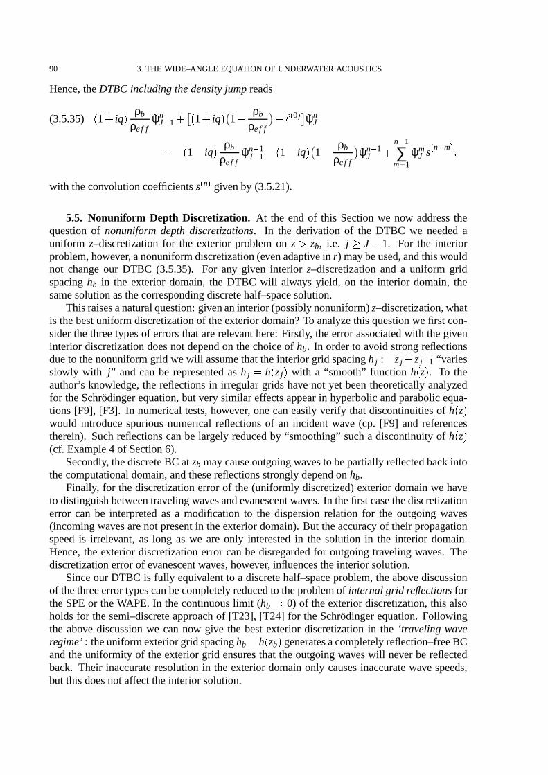
90 3. THE WIDE–ANGLE EQUATION OF UNDERWATER ACOUSTICS
Hence,theDTBCincludingthedensityjumpreads
(3.5.35) [ 1 diq ] ρb
ρef fψn
J e 1d [ 1 d
iq ] 1 X ρb
ρef fX 0~ ψn
J
WYX[ 1 X iq ] ρb
ρef fψne 1
J e 1 X[ 1 X iq ] 1 X ρb
ρef fψne 1
Jd ne 1
∑mq 1
ψmJ s ne m~ \
with theconvolutioncoefficientss n~ givenby (3.5.21).
5.5. Nonuniform Depth Discretization. At the endof this Sectionwe now addressthequestionof nonuniformdepthdiscretizations. In the derivation of the DTBC we neededauniform z–discretizationfor the exterior problemon z ^ zb, i.e. j ` J X 1. For the interiorproblem,however, anonuniformdiscretization(evenadaptivein r) maybeused,andthiswouldnot changeour DTBC (3.5.35). For any given interior z–discretizationand a uniform gridspacinghb in the exterior domain,the DTBC will always yield, on the interior domain,thesamesolutionasthecorrespondingdiscretehalf–spacesolution.
Thisraisesanaturalquestion:givenaninterior(possiblynonuniform)z–discretization,whatis thebestuniformdiscretizationof theexteriordomain?To analyzethis questionwefirst con-siderthethreetypesof errorsthatarerelevanthere:Firstly, theerrorassociatedwith thegiveninterior discretizationdoesnot dependon thechoiceof hb. In orderto avoid strongreflectionsdueto thenonuniformgrid wewill assumethattheinteriorgrid spacingh j : W zj X zj e 1 “variesslowly with j” andcanbe representedash j W h [ zj ] with a “smooth” function h [ z] . To theauthor’s knowledge,the reflectionsin irregular grids have not yet beentheoreticallyanalyzedfor theSchrodingerequation,but very similar effectsappearin hyperbolicandparabolicequa-tions [F9], [F3]. In numericaltests,however, onecaneasilyverify thatdiscontinuitiesof h [ z]would introducespuriousnumericalreflectionsof an incidentwave (cp. [F9] andreferencestherein). Suchreflectionscanbe largely reducedby “smoothing”sucha discontinuityof h [ z](cf. Example4 of Section6).
Secondly, thediscreteBC atzb maycauseoutgoingwavesto bepartially reflectedbackintothecomputationaldomain,andthesereflectionsstronglydependon hb.
Finally, for thediscretizationerrorof the (uniformly discretized)exterior domainwe haveto distinguishbetweentravelingwavesandevanescentwaves.In thefirst casethediscretizationerror can be interpretedas a modificationto the dispersionrelation for the outgoingwaves(incomingwavesarenot presentin theexterior domain).But theaccuracy of their propagationspeedis irrelevant, as long as we are only interestedin the solution in the interior domain.Hence,the exterior discretizationerror canbe disregardedfor outgoingtraveling waves. Thediscretizationerrorof evanescentwaves,however, influencestheinterior solution.
Sinceour DTBC is fully equivalentto a discretehalf–spaceproblem,theabove discussionof thethreeerrortypescanbecompletelyreducedto theproblemof internalgrid reflectionsfortheSPEor theWAPE. In thecontinuouslimit (hb 0) of theexterior discretization,this alsoholdsfor thesemi–discreteapproachof [T23], [T24] for theSchrodingerequation.Followingthe above discussionwe cannow give the bestexterior discretizationin the ‘tr avelingwaveregime’: theuniformexteriorgrid spacinghb W h [ zb ] generatesacompletelyreflection–freeBCandtheuniformity of theexterior grid ensuresthat theoutgoingwaveswill never bereflectedback. Their inaccurateresolutionin the exterior domainonly causesinaccuratewave speeds,but this doesnotaffect theinterior solution.

6. NUMERICAL EXAMPLES 91
This behaviour is numericallyverified in the simulationsof Section5 in [T24], whereauniformly spacedgrid wascomparedto the semi–discreteapproachfor the exterior domain.There,a Schrodingerequationwith a constantpotential is considered,and hencethe initialGaussianwavepacket consistsonly of travelingwavemodesin theexteriordomain.
In the‘evanescentwaveregime’, however, thepictureis not thatsimple,andit is notknownyet whetherthereexistsa existsa unique‘bestexterior discretization’.Our simulationsof thefollowingSection6 indicatethatit mayindeedbeadvantageousto useaDTBC thatcorrespondsto a finer exterior discretization,aslong astheinterior andexterior grid spacingsaregraduallymatchedto eachother.
6. Numerical Examples
In the first two examplesof this Sectionwe shall considerthe SPEand the WAPE forcomparingthenumericalresultfrom usingournew discreteTBCto thesolutionusingeitherthediscretizedTBCof ThomsonandMayfield[T26] or anabsorbinglayer. Dueto its construction,our DTBC yieldsexactly (up to round–off errors)thenumericalhalf–spacesolutionrestrictedto the computationalinterval s 0\ zb . The simulationwith discretizedTBCs requiresthe samenumericaleffort. However, their solutionmay(oncoarsegrids)stronglydeviatefrom thehalf–spacesolution.
In eachexamplewe usedtheGaussianbeamfrom [U18] asinitial data.Below we presenttheso–calledtransmissionloss X 10log10 p p p 2, wheretheacousticpressurep is calculatedfrom(3.1.3).
Example 1. This is a well–known benchmarkproblemfrom the literature[U18], [T20],[T26]. In this example the oceanregion (0 _ z _ 240m) with the uniform density ρw W1Z 0gcme 3 is modeledby theSPE(3.1.6). It containsno attenuationanda large densityjump(ρb W 2Z 1gcme 3) at the water–bottominterface. Hence,this problemprovidesa test of thetreatmentof thedensityjump in theTBCsappliedalongzb W 240m.
Thesourceof f W 100Hz is locatedat a waterdepthzs W 30m andthereceiver depthis atzr W 90m. Thesoundspeedprofile in wateris givenby c [ z]W 1498
d p 120 X zp c 60mse 1, andthesoundspeedin thebottomis cb W 1505mse 1. For our calculationsup to a maximumrangeof 20km we useda referencesoundspeedc0 W 1500mse 1 anda uniform computationalgridwith depthstep∆z W 2m andrangestep∆r W 5m (thesamestepsizeswereusedin [T26]).
In Figure3.5thesolid line is thesolutionwith ournew discreteTBC (3.5.35)andthedottedline is obtainedwith the discretizedTBC (3.5.3). The discretizedTBC clearly introducesasystematicphase–shifterror, which is roughly proportionalto ∆z. The discretizedTBC alsoproducesartificial oscillations(cf. thezoomedregion),while ournew DTBC yieldsthesmoothsolutionwith thesamenumericaleffort.
Figure3.6comparestheresultsof ournew discreteTBC (solid line) to thesolutionobtainedwith an absorbinglayer of 240m thickness(dottedline) anda homogeneousDirichlet BC atzmax W 480m. Hencethecomputationtook abouttwice aslong asby usingthediscreteTBC.In our experimentswe obtaineda bettermatchto the ‘exact’ half–spacesolutionby usingtheexponentialabsorptionprofile
αb [ z]W 10 exp 4z X zb
zmax X zbX 1 dB c λb \ zb _ z _ zmax\(3.6.1)
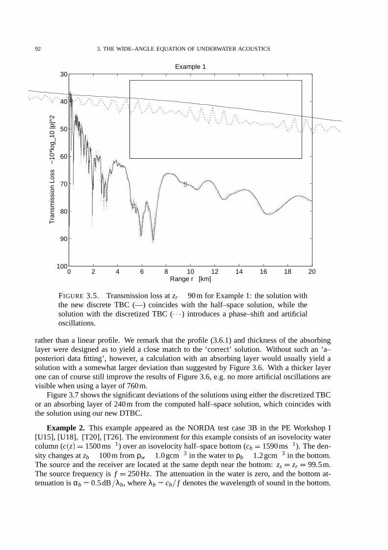
92 3. THE WIDE–ANGLE EQUATION OF UNDERWATER ACOUSTICS
0 2 4 6 8 10 12 14 16 18 20
30
40
50
60
70
80
90
100
Range r [km]
Tra
nsm
issi
on L
oss
−10
*log
_10
|p|^
2
Example 1
FIGURE 3.5. Transmissionlossat zr 90m for Example1: thesolutionwiththe new discreteTBC (—) coincideswith the half–spacesolution, while thesolution with the discretizedTBC ( ®®® ) introducesa phase–shiftandartificialoscillations.
ratherthana linear profile. We remarkthat the profile (3.6.1)andthicknessof the absorbinglayer weredesignedasto yield a closematchto the ‘correct’ solution. Without suchan ‘a–posterioridatafitting’, however, a calculationwith an absorbinglayer would usuallyyield asolutionwith a somewhat larger deviation thansuggestedby Figure3.6. With a thicker layeronecanof coursestill improve theresultsof Figure3.6,e.g.no moreartificial oscillationsarevisible whenusinga layerof 760m.
Figure3.7showsthesignificantdeviationsof thesolutionsusingeitherthediscretizedTBCor an absorbinglayer of 240m from the computedhalf–spacesolution,which coincideswiththesolutionusingour new DTBC.
Example 2. This exampleappearedas the NORDA test case3B in the PE WorkshopI[U15], [U18], [T20], [T26]. Theenvironmentfor this exampleconsistsof anisovelocitywatercolumn(c ¯ z° 1500ms± 1) overanisovelocityhalf–spacebottom(cb 1590ms± 1). Theden-sity changesat zb 100m from ρw 1² 0gcm± 3 in thewaterto ρb 1² 2gcm± 3 in thebottom.The sourceandthe receiver arelocatedat the samedepthnearthe bottom: zs zr 99² 5m.The sourcefrequency is f 250Hz. The attenuationin the wateris zero,andthe bottomat-tenuationis αb 0² 5dB ³ λb, whereλb cb ³ f denotesthewavelengthof soundin thebottom.
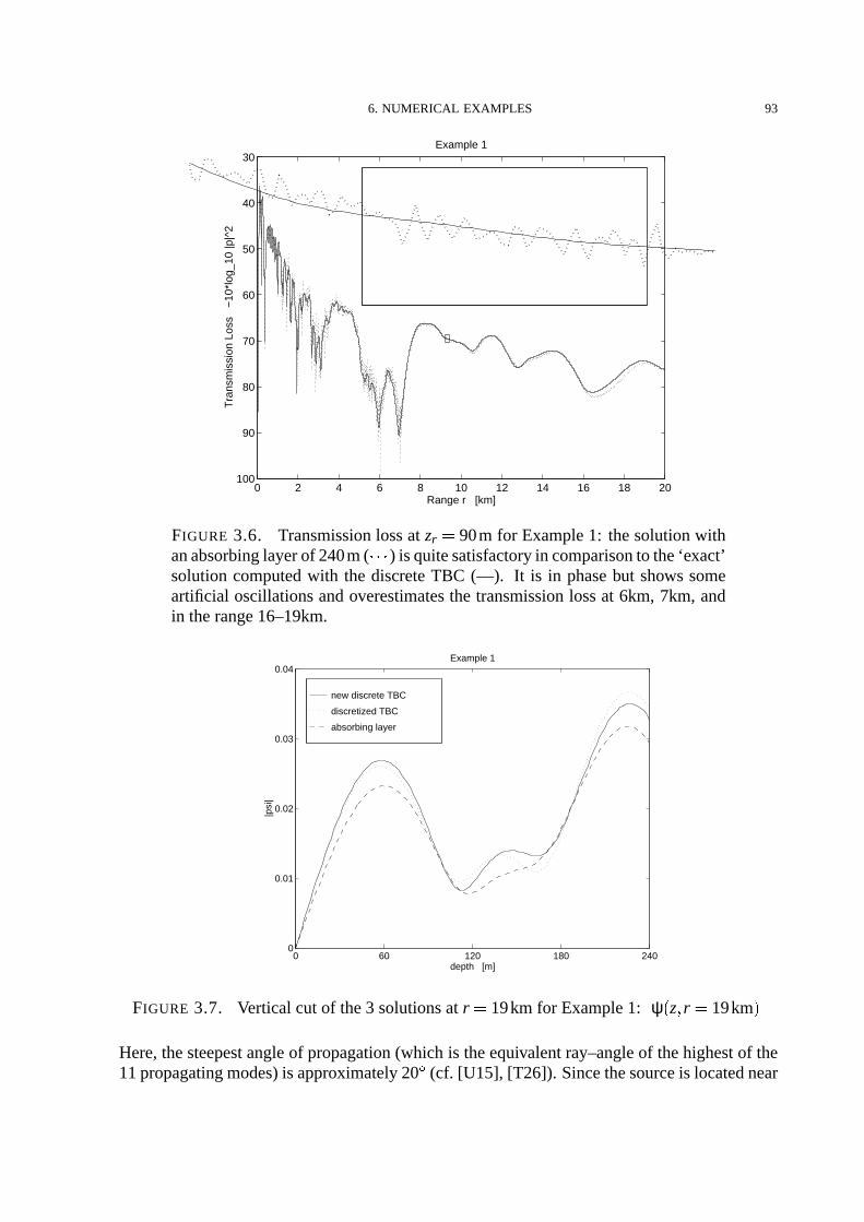
6. NUMERICAL EXAMPLES 93
0 2 4 6 8 10 12 14 16 18 20
30
40
50
60
70
80
90
100
Range r [km]
Tra
nsm
issi
on L
oss
−10
*log
_10
|p|^
2
Example 1
FIGURE 3.6. Transmissionlossat zr 90m for Example1: thesolutionwithanabsorbinglayerof 240m( ®?®® ) is quitesatisfactoryin comparisonto the‘exact’solutioncomputedwith the discreteTBC (—). It is in phasebut shows someartificial oscillationsandoverestimatesthe transmissionlossat 6km, 7km, andin therange16–19km.
new discrete TBC
discretized TBC
absorbing layer
0 60 120 180 2400
0.01
0.02
0.03
0.04Example 1
depth [m]
|psi
|
FIGURE 3.7. Verticalcut of the3 solutionsat r 19km for Example1: ´ ψ ¯ zµ r 19km°(´Here,thesteepestangleof propagation(which is theequivalentray–angleof thehighestof the11propagatingmodes)is approximately20¶ (cf. [U15], [T26]). Sincethesourceis locatednear

94 3. THE WIDE–ANGLE EQUATION OF UNDERWATER ACOUSTICS
thebottom,thehighermodesaresignificantlyexcited. Thereforethewide–anglecapabilityisimportanthereandwe usetheWAPE (3.1.8)(with thecoefficientsof Claerbout)to solve thisbenchmarkproblem.
The maximumrangeof interestis 10km andthe referencesoundspeedis chosenasc0 1500ms± 1. Thecalculationswerecarriedout usingthedepthstep∆z 0² 25m andthe rangestep∆r 2² 5m. Sincethe sourceis placedcloseto the bottom, the TBC wasapplied10mbelow theocean–bottominterface(thesamewasdonein [T26]).
new discrete TBCdiscretized TBC
5 6 7 8 9 10
60
70
80
90
100
Range r [km]
Tra
nsm
issi
on L
oss
−10
*log
_10
|p|^
2
Example 2
FIGURE 3.8. Transmissionlossatzr 99² 5m for Example2: thesolutionwiththenew discreteTBC coincideswith thehalf–spacesolution,while thesolutionwith the discretizedTBC still deviatessignificantlyfrom it for the chosendis-cretization.
The typical featureof this problemis the large destructive interferencenull at a rangeof7km. Figure3.8 comparesthe transmissionlossresultsfor thediscreteanddiscretizedTBCsin therangefrom 5 to 10km. In a secondcomparisonwe extendedthecomputationaldomainup to 200m. With the given bottomattenuationthis 100m layer is thick enoughto yield thereasonableapproximationshown in Figure3.9.
Figure 3.10 shows the deviation of the solutionswith the discretizedTBC and with theabsorbinglayerfrom thecomputedhalf–spacesolution,whichcoincideswith thesolutionusingour new discreteTBC.

6. NUMERICAL EXAMPLES 95
new discrete TBC
absorbing layer
5 6 7 8 9 10
60
70
80
90
100
Example 2
Range r [km]
Tra
nsm
issi
on L
oss
−10
*log
_10
|p|^
2
FIGURE 3.9. Transmissionlossat zr 99² 5m for Example2: in comparisonto theexacthalf–spacesolution,the truncationof thecomputationaldomainat200m (thegivenbottomattenuationthenrepresentsanabsorbinglayerof 100m)introducesaslightphaseshift.
new discrete TBC
discretized TBC
absorbing layer
0 20 40 60 80 1000
0.04
0.08
0.12
0.16Example 2
depth [m]
|psi
|
FIGURE 3.10. Verticalcut of the3 solutionsat r 7km for Example2: ´ ψ ¯ zµ r 7km°#´Example 3. In this examplewe illustratethe theoreticalfindingsof Section3 on coupled
models.We usethephysicalparametersof thefirst two examplesbut differentmodelsfor thewaterandthebottomregion.

96 3. THE WIDE–ANGLE EQUATION OF UNDERWATER ACOUSTICS
Westartwith consideringtheenvironmentof Example2 andcomparetheresultsof differentmodelcouplings.First we fix theWAPE of Claerbout(CWAPE; p0 1, p1 3
4, q1 14) in the
bottomandchooseadifferent(andin factbetter)rationalapproximation(GWAPE)for thewaterregionthatfulfils thecouplingcondition(3.3.9):p1 3q1. Thetwo remainingparametersp0, q1
arethendeterminedby minimizingtheapproximationerrorof ¯ 1 · λ ° 12 (in themaximumnorm)
over the interval ¸ 0² 0008µ 0² 103¹ , which containsthediscretespectrumof L: p0 1² 0000071,q1 0² 2501753.We comparethis approximationto thecaseof alsousingtheCWAPE in thewater. Furthermore,we show theresultswhenusingtheSPEin theseabottom(which clearlyviolates(3.3.9))andwhenusingtheSPEin bothregions.
GWAPE / CWAPE
CWAPE / CWAPE
CWAPE / SPE
SPE / SPE
7 8 9
60
70
80
90
100
Range r [km]
Tra
nsm
issi
on L
oss
−10
*log
_10
|p|^
2
Example 3
FIGURE 3.11. Transmissionloss at zr 99² 5m in several coupledmodels(waterandseabottom)for thesimulationof Example2.
Figure3.11displaysa comparisonof the transmissionlossfrom 6.5 to 9km for thesedif-ferentcouplings.It turnsout that thesolutionfor thecoupledGWAPE/CWAPE modelis verycloseto theoneusingtheCWAPE in bothmedia.While theCWAPE/SPEmodelviolatesthecoupling condition, it only deviatesfrom the above solutionsby a slight phase–shiftthat istypical for theSPEin this example(cp.alsothe“pure” SPEmodel).
Now we turn to the dissipation–freesituationof Example1 andfocusour attentionon aconservativediscretizationof coupledmodelsthatsatisfythecouplingconditionp1 ¯ z°³ q1 ¯ z° µ const, and hencepreserve the L2 ¯ IRº ; ¯ σρ ° ± 1dz° –norm (seeSection3). As a discrete

6. NUMERICAL EXAMPLES 97
analogueof (3.2.9)weobtainin thedissipation–freecase
(3.6.2) hD»kJ ± 1
∑j ¼ 0
ψnj
2
σρ j · 2
p21k0 ρef f
Im ¯ p1 · q1 ° ψnº 12
J ± 1 ½ iq1k ± 10 D»k ψn
J ± 1 ¾¾ ¯ p1 · q1 ° D»hψnº 1
2J ± 1 ½ iq1k ± 1
0 D»kD»hψnJ ± 1 µ
with ρ j ρ ¯ zj ° andσ p21 ³¿¯ p1 · p0q1 ° . Analogously, a discreteversionof (3.2.10)canbe
shown for thebottomregion j À J:
(3.6.3) hD»k∞
∑j ¼ J
ψnj
2
σbρb 2
¯ pb1 ° 2k0 ρef f
Im ¯ pb1 · qb
1 ° ψnº 12
J ± 1 ½ iqb1k ± 1
0 D»k ψnJ ± 1 ¾
¾ ¯ pb1 · qb
1 ° D»hψnº 12
J ± 1 ½ iqb1k ± 1
0 D»kD»hψnJ ± 1 µ
with σb ¯ pb1 ° 2 ³¿¯ pb
1 · pb0qb
1 ° . For coupledmodelsσ usuallytakesdifferentvaluesin thewaterand bottom regions. It follows from (3.6.2), (3.6.3) that the weighteddiscreteL2–norm onj Á IN0 is preserved:
Âψn  2 h
J ± 1
∑j ¼ 0
ψnj
2
σρ j½ h
∞
∑j ¼ J
ψnj
2
σbρb const(3.6.4)
providedthatthecouplingcondition(3.3.9)is fulfilled.Figure3.12illustratesthatthediscreteL2–norm(3.6.4)is conservedaslongasthecoupling
condition(3.3.9) is satisfied. In all four simulationswe usedthe WAPE of Claerboutfor thewaterregion anddifferentmodelsin theseabottom: only thehybrid WAPE–modelwith con-stantp1 ¯ z°³ q1 ¯ z° µ 3 renderstheschemeconservative (only for this numericalillustrationwechoosethevaluesp0 0² 6,q1 0² 2). A couplingto theSPE(like in [T20]) or to aWAPEinthebottomwith pb
1 ³ qb1 µb à 3 all yieldsa non–conservativescheme.We point out thatthese
schemesarenot only non–conservative for the particularnorm (3.6.4)but alsofor any otherweightedL2–norm.
In thesimulationsfor Figure3.12,thesecondsumof (3.6.4)(for theexteriorof thecompu-tationaldomain)wasevaluatedvia (3.6.3).
Example 4. In this examplewe illustrateour discussionfrom Subsection5.5 on the ‘bestuniformexterior discretization’ for thecaseof evanescentwaves. We want to answerthe fol-lowing question:givena uniform interiordiscretization,cantheresultfrom aglobally uniformz–discretizationbe improvedby choosinga finer exterior z–discretization,or, equivalently, byusinga DTBC thatcorrespondsto suchafinerdiscretization?
As amodelproblemfor thistestweconsidertheSPE(3.1.6)onz Ä 0µ r Ä 0 with ahomoge-neousDirichlet BC atz 0, k0 2m± 1 andthe“potentialwell” V ¯ z° 0µ 0 Å z Å zb 100m,V ¯ z° Vb 0² 3µ z Ä zb. In thisexample,planewaveswith awavenumberk Å kcrit ÇÆ 1² 2m± 1
areevanescentin theexterior domainz Ä zb, andk Ä kcrit transmitsa traveling wave into theexterior. We chooseheretheGaussianbeamexp ¯ ikz · 0² 003m± 2 ¯ z · 50m° 2 ° with k 1m± 1
asaninitial condition.For this choiceof k ‘most’ of theFouriercomponentsof this wave cor-respondto evanescentmodesin thebottom. Hence,this wave will bepredominantlyreflectedbackinto theinteriordomain.

98 3. THE WIDE–ANGLE EQUATION OF UNDERWATER ACOUSTICS
WAPE: p_1/q_1=3
SPE
WAPE: p_1/q_1=3.25
WAPE: p_1/q_1=2.75
0 2 4 6 8 10 12 14 16 18 200.95
1
1.05
1.1
1.15
1.2
1.25
1.3
1.35
1.4
Range r [km]
(nor
mal
ized
) w
eigh
ted
L2−
norm
Example 3
FIGURE 3.12. CoupledWAPE–modelsconserve thediscreteL2–norm(3.6.4)only whensatisfyingthecouplingconditionp1 ³ q1 µ const(—).
Figure3.13comparestheeffectof choosingdifferent(uniformandnonuniform)z–discreti-zations.We show the resultsof this simulationat the ranger 200m whenthewave packethasbeenreflectedbackfrom thewater–bottominterface.Thesolid line wasobtainedwith theuniform z–discretizationh0 0² 05m, andit will serve asour ‘exact’ referencesolution. Thedashedline shows the solutionwith the uniform grid spacingh1 0² 25m. In the followingcomparisonswe will keepthis coarserinterior grid and will vary the uniform exterior grid.Following our discussionfrom Subsection5.5,we useda gradualtransitionbetweenthesetwogrid spacingsin thedepthinterval 100 · 110m (piecewiselineargrid spacingfunctionh ¯ z° ).
The dottedcurve of Figure 3.13 gives the resultswith the finer exterior z–discretizationh2 0² 1m. Closeto the seabottomit shows significantimprovementsover the uniform dis-cretizationwith h1. In the interval 0 Å z Å 60m both curvesalmostcoincideas the interiordiscretizationerroris dominantthere,andit impliesinaccuratewavespeedsthatarereflectedintheclearlyvisible phaseshift. Thedottedcurve still exhibits this phaseshift up to theseabot-tom at 100m, but for thedashedcurve theerror in the interval 80m Å z Å 100m is dominatedby the effect of the exterior discretization. It thusseemsthat the effect of the reducedexte-rior discretizationerror (dueto the finer exterior discretization)mayoutweigh(in the interiordomain!)theadditionalreflectionerrorsincurredby thenonuniformgrid.
TheL2 ¯ 0µ 100° –errors(w.r.t. thesolidcurve)of thesolutionswith theuniformh1–discretiza-tion andthenonuniformh1 ³ h2–discretizationare,respectively, 0² 0370and0² 0267. Usinganeven finer exterior discretizationdoesnot seemto improve the resultmuchfurther (L2–error

6. NUMERICAL EXAMPLES 99
uniform dz=0.05m uniform dz=0.25m nonuniform dz=0.25−0.1m
0 20 40 60 80 1000
0.2
0.4
0.6
0.8
1Example 4
depth [m]
|psi
|
FIGURE 3.13. The ‘bestuniform exterior z–discretization’maybe finer thanthe interior discretization. Vertical cut of the threesolutionsat r 200m forExample4: thesolution( ®®?® ) calculatedon a nonuniformgrid (finer grid in theexteriordomainthanin theinterior) is moreaccuratein theinteriordomainthanthesolutionobtainedon a uniformly coarsegrid (– – –). Thereferencesolution(—) wascalculatedon auniformly finegrid.
0² 0266for theh1 ³ h0–discretization).A finer exterior discretizationwould, however, requireathicker region to adaptthetwo grids.
We thusconcludethatfinerexteriordiscretizationsmayindeedbeadvantageousin thecaseof evanescentwaves, and for large rangestheseare the importantmodesin the consideredapplicationsof underwateracoustics.

100 3. THE WIDE–ANGLE EQUATION OF UNDERWATER ACOUSTICS
Conclusionsand Perspectives
Wehavederivedanew discretization(discreteTBC) of theanalyticTBC for theconvection–diffusionequationandSchrodinger–typepseudo–differentialevolution equationsin onespacedimension.It is of discreteconvolution form in t involving theboundarydatafrom all thepasttime levels.
TheconvolutioncoefficientssÈ nÉ canbecalculatedvia a simplethree–termrecurrencerela-tion andthey decaylikeO ¯ n± 3Ê 2 ° . Sinceour new DTBC hasthesameconvolutionstructureasexisting discretizations,it requiresthesamecomputationaleffort but improvestwo shortcom-ings: DTBCsaremore accurate(in fact,asaccurateasthediscretewhole–spaceproblem)andthey retainthestabilityof theunderlyingfinite differencescheme.
Theunderwateracousticscommunitytookagreatinterestin theresultsof Chapter3. Espe-cially the(continuous)TBC for anelasticbottomcaughttheir attentionandwill bediscretizedandimplementedin existingnumericalcodes.Our commentson themathematicaldifficulty ofcouplingdifferentmodelsfor thewaterandbottomregion arealsoof interest. In underwateracousticsthe computationsmust be very fast and thereforecoarsegrids arepreferredwhichmakestheusageof DTBCsadvantageous.
We point out that the superiorityof DTBCs over otherdiscretizationsof TBCs is not re-strictedto the presentedspecialtypesof partial differentialequationsor to our particularin-terior discretizationscheme(seee.g. [T1], [T2], [T3], [T4], [T5], [T10], [P2], [T11]). Thecrucial point of our derivation was to find the inverse Ë –transformationof the transformedDTBC explicitly. In moregeneralapplications,e.g.2D transientSchrodingerequation(corre-spondsto 3D–problemsin underwateracoustics),systemsof equationsor high–orderschemes,it might be necessaryto useour secondapproachof deriving the recurrencerelation for theconvolutioncoefficientsor to calculatetheconvolutioncoefficientsthroughanumericalinverseË –transformation(seeSection4 in Chapter1), but this doesnot changethe efficiency of thepresentedmethod.Moreover, in thegeneralcasetheDTBC will benonlocalin morethanonevariableandonehasto seekfor approximatelocal BCsthat leadto a stablescheme.As a gen-eralphilosophy, DTBCsshouldbeusedwheneverhighly accuratesolutionsareimportant.Ourstrategieshave alreadybeenadaptedby a Princetonworkgroupto systemsof wave equationsfor materialswith cracks.
Topics of future researchinclude DTBCs for higher order schemes, e.g. the Numerovscheme[U11], or moreefficient algorithmslike split–stepPade schemes[U9] in the appli-cationto underwateracoustics.Moreover we will usethe ideasof Section3 in Chapter1 andderiveaDTBC for theWAPE in thecasethatthestartingfield is notsupportedinsidethewaterregion (which is thecomputationaldomain). We intendto apply the ideasof Markowich andPoupaud[F5] in order to derive a finite differencediscretizationdirectly for the squarerootoperatorÆ 1 · L from Chapter3. Furthermorewe searchfor a conservative formulationof theelastic/fluidcouplingwhich is neededfor stablediscretizationsandasguidancefor deriving aDTBC for anelasticbottom.
101
102 CONCLUSIONSAND PERSPECTIVES
We will constructDTBCsfor situationsin which theexterior problemshave variablecoef-ficientsbut still areexplicitly solvable. For a linearCrank–Nicolson–typeschemeto solve theradialSchrodinger–Poissonsystempreservingboth theenergy andthemass[F6] we shall tryto designan appropriateboundaryconditionat the origin anda DTBC for r Ì ∞ [F7]. Alsowe will designDTBCsfor theSchrodingerequationwith a linearpotentialtermin theexteriordomain.This derivationis basedon theknowledgeof theasymptoticbehaviour of solutionstoa discreteAiry equation(cf. [E4], [E5]). This problemarisesin underwateracousticsin [T8]andin “parabolicequation”predictionsfor radarpropagationin thetroposphere[T13].
Finally to remedythe deficiency that our DTBC is nonlocal in the time variablewhichis noticeableespeciallyin long–timecalculationswe constructnew approximative transparentboundaryconditions[D1]. TheseBCsareanefficient convolution by anexponentialapproxi-mation:only onesimpleupdateis neededin eachtimestepto computethediscreteconvolution.We alsoprovecriteriafor thenumericalstabilityof theresultingIBVP.

Appendix
The Laplace Transformation
Herewe discussthe Laplacetransformationf f ¯ s° of a function f f ¯ t ° andpresentsomeelementaryresults.In this thesistheLaplacetransformationwasusedto explicitly solvetheexterior problemsin orderto derive thecontinuousTBCs.
DEFINITION L.1 (Laplacetransformation[S3]). If for a function f : IR» Ì IC thereexistsaσ Á IR, suchthattheintegral
ÍÏÎf п¯ s° : f ¯ s° : ∞
0f ¯ t ° e± st dt µ(L.1)
existsfor all s Á IC with Res Ä σ, then f ¯ s° is theLaplacetransformationof f .
Themostimportantpropertyof theLaplacetransformationis therelationshipbetweende-rivativeandtransformation:
THEOREM L.1 (DifferentiationTheorem[S3]). If the function f : IR» Ì IC is differentiableandtheLaplacetransformationof f Ñ exists,thenthelimit
f ¯ 0½ ° : limt Ò 0º f ¯ t °µ
existsandfor Res Ä σ theLaplacetransformationof f Ñ fulfilsÍÏÎf Ñ Ð¿¯ s° s f ¯ s°U· f ¯ 0½ °²(L.2)
Theinitial valuesenterinto thetransformationof thederivative.Theessentialrule for deriving thecontinuousTBCsis theLaplacetransformationof acon-
volution f Ó g of two functions f µ g : IR» Ì IC which is definedas
¯ f Ó g°B¯ t ° t
0f ¯ τ ° g ¯ t · τ ° dτ ²
THEOREM L.2 (Convolution Theorem[S3]). If theLaplacetransformation(L.1) existsforthefunctionsf µ g : IR» Ì IC andat leastoneLaplaceintegral is absolutelyconvergent thenwehave ÍÏÎ
f Ó gп¯ s° f ¯ s° g ¯ s°²(L.3)
It is alsonecessaryto havea link betweennormsin thephysicalandtransformedspace:
THEOREM L.3 (Plancherel’s Theorem[M5]) . If thefunction f : IR» Ì IC is continuousandsatisfiesan estimate
´ f ¯ t °(´ 2 Ô Ceσt µ t À 0µ103

104 APPENDIX
for somereal constantsC, σ, thentheLaplacetransformationof f (L.1) is ananalyticfunctionfor Res Ä σ and
∞
0e± 2ηt ´ f ¯ t °(´ 2 dt 1
2π
∞
± ∞f ¯ η ½ iξ ° 2
dξ µ η Ä σ ²(L.4)
holds.
The InverseLaplaceTransformation
Here we shortly give the basicfactsaboutthe inverseLaplacetransformationwhich areneededfor statingthecontinuousTBC in physicalvariables.The inverseLaplacetransforma-tion is givenasfollows:
THEOREM L.4 (InverseLaplacetransformation[S3]). Theinverseof theLaplacetransfor-mationis givenby theBromwich integral
Í ± 1 f ¯ t ° 12πi
γ º i∞
γ ± i∞est f ¯ s° dsµ(IL.1)
where γ is a vertical contourin thecomplex planechosensuch thatall singularitiesof f ¯ s° areto theleft of it.
As we haveseenin TheoremL.2 therule for inversetransformingaproductis simply
Í ± 1 f g ¯ t ° t
0f ¯ τ ° g ¯ t · τ ° dτ ²(IL.2)
Finally wepresentacollectionof usedinverseLaplace–transformationrulesfrom [S2].
Í ± 1 1s· 1
c ½ s 1 · e± ct µ s Ä maxÎ0µ· cÐ(IL.3)
Í ± 1 Æ s · γ · Æ s 12Æ π
¯ 1 · eγt ° t ± 32(IL.4)
Í ± 1 1
Æ s 1
Æ πt ± 1
2(IL.5)
Í ± 1 f ¯ s ½ σ ° f ¯ t ° e± σt(IL.6)
Í ± 1 s f ¯ s ½ σ ° ddt
f ¯ t ° e± σt µ if ψ ¯ 0° 0(IL.7)
Í ± 1 1
Æ sei Õ α Õ s 1
Æ πte
α4t(IL.8)

THE Ö –TRANSFORMATION 105
The Ë –Transformation
The main tool of this work is the Ë –transformationwhich is the discreteanalogueof theLaplace–transformation.The Ë –transformationcan be appliedto the solution of linear dif-ferenceequationsin order to reducethe solutionsof suchequationsinto thoseof algebraicequationsin the complex z–plane. In this theseswe usedit to explicitly solve the finite dif-ferenceschemesin theexterior domainin orderto constructthediscretetransparentboundaryconditions.The Ë –transformationis describedin moredetail in [S3], [S6], [S8]. It is definedin thefollowing way:
DEFINITION Z.1 ( Ë –transformation[S3]). Theformalconnectionbetweenasequenceandacomplex functiongivenby thecorrespondence
Ë Îfn Ð f ¯ z° : ∞
∑n¼ 0
fnz± n µ z Á ICµ ´ z3Ä Rf µ(Z.1)
is called Ë –transformation.Thefunction f ¯ z° is called Ë –transformationof thesequenceÎ
fn Ð ,n 0µ 1µ?²²² andRf À 0 denotestheradiusof convergence.
Thediscreteanalogueof theDifferentiationTheoremfor theLaplacetransformationis theshiftingtheorem:
THEOREM Z.1 (Shifting Theorem[S3]). If thesequenceÎ
fn Ð is exponentiallybounded,i.e.thereexistC Ä 0 andc0 such that
´ fn ´ Ô Cec0n µ n 0µ 1µ²²² µthenthe Ë –transformationf ¯ z° is givenbytheLaurentseries(Z.1)andfor theshiftedsequenceÎgn Ð with gn fnº 1 holds
Ë Îfnº 1 Ð zf ¯ z°U· zf0 ²(Z.2)
Theinitial valuesenterinto thetransformationof theshiftedsequence.As a usefulconse-quenceof theshifting theoremwehave:
Ë Îfnº 1 × fn Ð ¯ z × 1° f ¯ z°U· zf0 ²(Z.3)
Theconvolution fn Ó gn of two sequencesÎ
fn Ð ,Îgn Ð , n 0µ 1µ²?²² is definedby ∑n
k¼ 0 fkgn± k.For the Ë –transformationof a convolution of two sequenceswe formulatethefollowing theo-rem:
THEOREM Z.2 ( [S8]). If f ¯ z° Ë Îfn Ð existsfor ´ z3Ä Rf À 0 andg ¯ z° Ë Î
gn Ð for ´ z3ÄRg À 0, thentherealsoexists Ë Î
fn Ó gn Ð for ´ zAÄ max Rf µ Rg ° with
Ë Îfn Ó gn Ð f ¯ z° g ¯ z°²(Z.4)
Note that (Z.4) is nothing elsebut an expresssionfor the Cauchyproductof two powerseries.We furtherneedthe Ë –transformationof aproductof two sequences.
THEOREM Z.3 (Complex ConvolutionTheorem[S8]). If f ¯ z° Ë Îfn Ð existsfor ´ z4Ä Rf À
0 and g ¯ z° Ë Îgn Ð for ´ z#Ä Rg À 0, thenthere also exists Ë Î
fngn Ð for ´ zBÄ Rf Rg and thefollowing relationholds:
Ë Îfngn Ð 1
2πi Ø f ¯ ξ ° gzξ
ξ ± 1dξ ²(Z.5)

106 APPENDIX
Theintegration pathis thecircle Ù aroundtheorigin: ξ r eiϕ, Rf Å r Åt´ zÚ³ Rg, 0 Ô ϕ Ô 2π(if Rg 0 : Rf Å r Å ∞).
As aconsequenceoneobtainsimmediatelyPlancherel’s theoremfor the Ë –transformation:
THEOREM Z.4 (Plancherel’s Theorem[S3]). If f ¯ z° Ë Îfn Ð exists for ´ z(Ä Rf À 0 and
g ¯ z° Ë Îgn Ð for ´ z=Ä Rg À 0 with Rf Rg Å 1. Thenthere alsoexists Ë Î
fn gn Ð for ´ z=Ä Rf Rg
andthefollowing relationholds:∞
∑n¼ 0
fn gn Ë Îfn gn п¯ z 1° 1
2π
2π
0f ¯ r eiϕ ° g
eiϕ
rdϕ ²(Z.6)
Theintegration path is thecircle Ù definedby Rf Å r Å 1³ Rg (if Rg 0: Rf Å r Å ∞). Espe-cially, if Rf Å 1, Rg Å 1 thenr 1 canbechosento obtain:
∞
∑n¼ 0
fn gn 12π
2π
0f ¯ eiϕ ° g ¯ eiϕ ° dϕ ²(Z.7)
Notethat g ¯ z° is not the Ë –transformationof gn, but Ë Îgn п¯ z° g ¯ z° holds.
The Inverse Ë –Transformation
Now we presentthebasicrulesfor calculatingthe inverseË –transformationwhich arees-sentialfor formulatingthediscretetransparentboundaryconditions.
THEOREM Z.5 (InverseË –transformation[S3]). IfÎ
fn Ð is an exponentiallyboundedse-quenceand f ¯ z° the correspondingË –transformationthen the inverse Ë –transformationisgivenby
fn Ë ± 1 f ¯ z° 12πi Ø f ¯ z° zn± 1dzµ n 0µ 1µ²²?²4µ(IZ.1)
where Ù denotesa circlearoundtheorigin with sufficientlylarge radius.
Otherinversionformulascanbeobtainedby usingthefact that f ¯ z± 1° is a Taylor seriesorif f ¯ z° is a rationalfunction of z, analyticat ∞ (cf. Section1.3 in [S6]). The most importantformulais the inverse Ë –transformationof a product:
Ë ± 1 f ¯ z° g ¯ z° fn Ó gn n
∑k¼ 0
fk gn± k µ(IZ.2)
which is thediscreteanalogueof (IL.2).
THEOREM Z.6 (Initial ValueTheorem[S3]). If f ¯ z° Ë Îfn Ð existsthen
f0 limzÒ ∞
f ¯ z°²(IZ.3)
z cantendto ∞ on thereal axisor on an arbitrary path,since f ¯ z° is analyticat z ∞.
This theorem,whenrepeatedlyappliedto f ¯ z° , f ¯ z°U· f0, f ¯ z°U· f0 · f1z± 1, etc.,providesa methodfor theinversionof the Ë –transformation:
fn limzÒ ∞
zn f ¯ z°· n± 1
∑k¼ 0
fkz± k µ n 0µ 1µ 2µ²²² ²(IZ.4)
THE INVERSE Ö –TRANSFORMATION 107
Below we presentsomeinverseË –transformationrulesfrom [S3], [S6], [S8] thatwe usedbefore:
Ë ± 1 Î 1Ð δ0n µ(IZ.5)
Ë ± 1 1z δ1
n µ ´ zAÄ 1µ(IZ.6)
Ë ± 1 zz · a an µ ´ z3ÄI´ a ´AÄ 0µ(IZ.7)
Ë ± 1 1z · a a± 1 ¯ an · δ0
n °µ ´ zAÄ*´ a ´3Ä 0µ(IZ.8)
andfor 0 Å θ Å 1 holds:
Ë ± 1 12 ¯ θz ½ 1 · θ ° · 1
2 ¯ 1 · θ ° · 1 · θθ
n · δ0n µ ´ z3Ä 1 · θ
θµ(IZ.9)
Ë ± 1 z · 12 ¯ θz ½ 1 · θ ° 1
2θδ0
n ½ 12θ ¯ 1 · θ ° · 1 · θ
θ
n · δ0n µ ´ z3Ä 1 · θ
θ²(IZ.10)
Fromthegeneratingfunctionof theLegendrepolynomialsPn [S4] weseethat
Ë ± 1 z
z2 · 2µz½ 1 Pn ¯ µ°µ ´ z3Ä R max ´ z1 ´ÛµJ´ z2 ´ µ(IZ.11)
holdsandintroducingthescalingvariableλ weobtainfor Pn ¯ µ° : λ ± nPn ¯ µ°Ë ± 1 λz
¯ λz° 2 · 2µλz ½ 1 Pn ¯ µ°µ ´ z3Ä R max λ ± 1z1 µ λ ± 1z2 ²(IZ.12)
Herez1, z2 denotethezerosof thedenominatorin (IZ.11).

108 APPENDIX
Bibliography
Programcodes
[C1] D.E. Amos,Algorithm644: A PortablePackage for BesselFunctionsof a Complex ArgumentandNonneg-ativeOrder, ACM Trans.Math.Software12 (1986),265–273.
[C2] D.E. Amos,Remarkon Algorithm644: “A PortablePackage for BesselFunctionsof a Complex ArgumentandNonnegativeOrder” , ACM Trans.Math.Software16 (1990),404.
[C3] D.E. Amos,A RemarkonAlgorithm644: A PortablePackagefor BesselFunctionsof a Complex ArgumentandNonnegativeOrder, ACM Trans.Math.Software21 (1995),388–393.
[C4] W. Gautschi,Algorithm259— Legendre functionsfor argumentslarger thanone, Comm.ACM 8 (1965),488–492.
[C5] J.N.LynessandG. Sande,Algorithm413: ENTCAFandENTCRE:Evaluationof NormalizedTaylor Coef-ficientsof an AnalyticFunction, Comm.ACM 14 (1971),669–675.
DiscreteApproachfor Artificial BCs
[D1] A. Arnold, M. EhrhardtandI. Sofronov, work in progress.[D2] B. EngquistandA. Majda, RadiationBoundaryConditionsfor Acousticand Elastic WaveCalculations,
Comm.PureAppl. Math.32 (1979),313–357.[D3] L. Halpern,AbsorbingBoundaryConditionsfor theDiscretizationSchemesfor theOne–DimensionalWave
Equation, Math.Comp.38 (1982),415–429.[D4] G. Lill, DiskreteRandbedingungenan kunstlichenRandern, Dissertation,TechnischeHochschuleDarm-
stadt,1992.[D5] C.W. Rowley andT. Colonius,DiscretelyNonreflectingBoundaryConditionsfor Linear HyperbolicSys-
tems, J.Comp.Phys.157(2000),500–538.[D6] L. Wagatha,OnBoundaryConditionsfor theNumericalSimulationof WavePropagation, Appl. Num.Math.
1 (1985),309–314.[D7] J.C.Wilson,Derivationof boundaryconditionsfor theartificial boundariesassociatedwith thesolutionof
certaintimedependentproblemsbyLax–Wendroff typedifferenceschemes, Proc.Edinb. Math.Soc.II. Ser.25 (1982),1–18.
Differ enceEquations
[E1] S.N.Elaydi, An introductionto differenceequations, UndergraduateTexts in Mathematics,Springer, NewYork, 1996.
[E2] W. Gautschi,Computationalaspectsof three–termrecurrencerelations, SIAM Rev. 9 (1967),24–82.[E3] R.E.Mickens,DifferenceEquations:TheoryandApplications, 2nded.,VanNostrandReinhold,New York,
1990.[E4] R.E.Mickens,Asymptoticpropertiesof solutionsto two discreteAiry equations, J.Dif ferenceEqu.Appl. 3
(1998),231–239.[E5] R.E.Mickens,AsymptoticSolutionsto a DiscreteAiry equation, to bepublishedin: J.DifferenceEqu.Appl.
(2001).
109
110 BIBLIOGRAPHY
Finite Differ enceSchemes
[F1] E.Becache,F. Collino,M. KernandP. Joly, Higherordernumericalschemesfor theparaxialwaveequation,MathematicalMethodsin GeophysicalImagingIII, 1995.
[F2] E. Hairer andG. Wanner, Solvingordinary differential equationsII: Stiff and differential-algebraic prob-lems, SpringerSeriesin ComputationalMathematics14,2ndrev. ed.,Springer-Verlag(1996).
[F3] T.A. Manteuffel andA.B. White Jr., Thenumericalsolutionof secondorder boundaryvalueproblemsonnonuniformmeshes, Math.Comput.47 (1986),511–535.
[F4] P.A. Markowich, P. PietraandC. Pohl,Numericalapproximationof quadratic observablesof Schrodinger–typeequationsin thesemi-classicallimit, Numer. Math.81 (1999),595–630.
[F5] P.A. Markowich,F. Poupaud,ThePseudo–DifferentialApproach to Finite DifferencesRevisited, Calcolo36(1999),161–186.
[F6] C. RinghoferandJ. Soler, DiscreteSchrodinger–PoissonSystemspreservingEnergy and Mass, AppliedMathematicsLetters,13 (2000),27-32.
[F7] M. Ehrhardt,C. Ringhofer, E. Ruiz–Arriola and J. Soler, NumericalAnalysisof Discrete Schrodinger–PoissonSystemspreservingEnergyandMass, in preparation.
[F8] J.C.Strikwerda,Finite DifferenceSchemesandPartial Differential Equations, Wadsworth & Brooks/Cole,1989.
[F9] R.Vichnevetsky, Wavepropagationandreflectionin irregular gridsfor hyperbolicequations, Appl. Numer.Math.3 (1987),133–166.
[F10] A. Zisowsky, Entwurfund ImplementierungeinesVerfahrensfur die transienteAnalysefluider stochastis-cherPetri–Netze, MastersThesis,TechnischeUniversitatBerlin, 1998.
Mathematical Analysis
[M1] N. Dunford andJ.T. Schwartz, Linear Operators, Part II: SelfAdjont Operators in Hilbert Space, JohnWiley IntersciencePublishers,New York, 1963.
[M2] G. Gripenberg, S.-O.LondenandO. Staffans,Volterra integral andfunctionalequations, EncyclopediaofMathematicsandIts Applications,34.CambridgeUniv. Press,Cambridge,1990.
[M3] H. Heuser, GewohnlicheDifferentialgleichungen: Einfuhrungin Lehre undGebrauch, Teubner, Stuttgart,1989.
[M4] L. Hormander, The analysisof linear partial differential operators III: Pseudo–differential operators,GrundlehrenderMathematischenWissenschaften274,Springer–Verlag,Berlin, 1985.
[M5] H.-O. KreissundJ.Lorenz,Initial–BoundaryValueProblemsandtheNavier–StokesEquations, AcademicPress,1989.
[M6] J.E.Lagnese,General boundaryvalueproblemsfor differential equationsof Sobolev type, SIAM J. Math.Anal. 3 (1972),105–119.
[M7] M. ReedandB. Simon,Methodsof ModernMathematicalPhysics,Part I: FunctionalAnalysis, AcademicPress,New York, 3rded. 1987.
Artificial Boundary Conditions for Parabolic Equations
[P1] E.Dubach,Artificial boundaryconditionsfor diffusionequations:Numericalstudy, J.Comput.Appl. Math.70 (1996),127–144.
[P2] M. Ehrhardt,DiscreteTransparentBoundaryConditionsfor Parabolic Equations, Z. Angew. Math.Mech.77 (1997)S2,543–544.
[P3] L. Halpern,Artificial BC’s for theLinearAdvectionDiffusionEquation, Math.Comp.46 (1986),425–438.[P4] L. HalpernandJ. Rauch,Absorbingboundaryconditionsfor diffusionequations, Num. Math. 71 (1995),
185–224.

BIBLIOGRAPHY 111
[P5] J.-P. Loheac,An Artificial BoundaryConditionfor an Advection–DiffusionProblem, Math.MethodsAppl.Sci.14 (1991),155–175.
[P6] J.-P. Loheac, In– and Out–Flow Artificial Boundary Conditions for Advection–Diffusion Equations,Z. Angew. Math.Mech.76 (1996)S5,309–310.
[P7] K. WolterandA. Zisowsky, NumericalSolutionof SecondOrderFluid StochasticPetri Netswith Reflectingand Transparent BoundaryConditions, submittedto: Proc.of the 11th Int. Conf. on Modell. Techn.andToolsfor Comp.PerformanceEvaluation,Schaumburg, Illinois, USA (2000).
SpecialFunctions and Transformation
[S1] M. Abramowitz and I.A. Stegun, Handbookof MathematicalFunctions, National Bureauof Standards,AppliedMath.Series#55,DoverPublications,1965.
[S2] BatemanManuscriptProject, Tablesof IntegralTransforms,vol. 1, McGraw–Hill, 1954.[S3] G. Doetsch,AnleitungzumpraktischenGebrauch der Laplace-Transformationundder Z-Transformation,
R. Oldenburg VerlagMunchen,Wien,3. Auflage1967.[S4] N.N. Lebedev, SpecialFunctionsandtheir Applications, SelectedRussianPublicationsin theMathematical
Sciences,Prentice–Hall,1965.[S5] H.J.Nussbaumer, FastFourier transformandconvolutionalgorithms, SpringerSeriesin InformationSci-
encesVol. 2. Springer–Verlag,1981.[S6] E.I. Jury, TheoryandApplicationof thez-TransformMethod, Wiley & Sons,New York, 1964.[S7] G. Szego, OrthogonalPolynomials, Amer. Math.Soc.ColloquiumPublications23,3rd ed.1967.[S8] R. Vich, Z–Transformation,TheorieundAnwendung, VerlagTechnikBerlin, 1964.
Transparent Boundary Conditions
[T1] A. Arnold, NumericallyAbsorbingBoundaryConditionsfor QuantumEvolutionEquations, VLSI Design6 (1998),313–319.
[T2] A. Arnold andM. Ehrhardt,A New DiscreteTransparentBoundaryConditionfor Standard andWideAngle“Parabolic” Equationsin UnderwaterAcoustics, Proceedingsof the “Third InternationalConferenceonTheoreticalandComputationalAcoustics”,Newark,New Jersey, USA, 1997,623–635.
[T3] A. Arnold andM. Ehrhardt,Discretetransparentboundaryconditionsfor wideangleparabolic equationsin underwateracoustics, J.Comp.Phys.145(1998),611–638.
[T4] A. Arnold andM. Ehrhardt,DiscreteTransparentBoundaryConditionsfor WideAngleParabolicEquationsin UnderwaterAcoustics, Proceedingsof the “Fourth EuropeanConferenceon Underwater Acoustics”,Rome,Italy, 1998,769–774.
[T5] A. Arnold,Mathematicalconceptsof openquantumboundaryconditions, to appearin: Transp.TheoryStat.Phys.,2000.
[T6] V.A. Baskakov andA.V. Popov, Implementationof transparent boundariesfor numericalsolutionof theSchrodinger equation, Wave Motion 14 (1991),123–128.
[T7] C.H. Bruneauand L. Di Menza,Conditionsaux limites transparenteset artificielles pour l’ equationdeSchrodinger endimension1 d’espace, C. R. Acad.Sci.Paris,Ser. I 320(1995),89–94.
[T8] T.W. Dawson,D.J.ThomsonandG.H.Brooke,Non–localboundaryconditionsfor acousticPEpredictionsinvolving inhomogeneouslayers, in 3rd EuropeanConferenceon UnderwaterAcoustics,FORTH–IACM,Heraklion,1996,pp.183–188.
[T9] L. Di Menza,Approximationsnumeriquesd’equationsdeSchrodinger nonlineairesetdemodelesassocies,Ph.D.thesis,UniversiteBordeauxI, 1995.
[T10] J.DouglasJr., J.E.Santos,D. SheenandL.S.Bennethum,Frequencydomaintreatmentof one–dimensionalscalarwaves, Math.Mod. andMeth. in Appl. Sc.3 (1993),171–194.
[T11] M. Ehrhardt,DiscreteTransparentBoundaryConditionsfor General Schrodinger–TypeEquations, VLSIDesign9 (1999),325–338.
[T12] J.R.HellumsandW.R.Frensley, Non–Markovianopen–systemboundaryconditionsfor thetime–dependentSchrodinger equation, Phys.Rev. B 49 (1994),2904–2906.
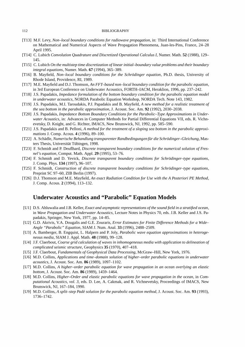
112 BIBLIOGRAPHY
[T13] M.F. Levy, Non–localboundaryconditionsfor radiowavepropagation, in: Third InternationalConferenceon MathematicalandNumericalAspectsof Wave PropagationPhenomena,Juan-les-Pins,France,24–28April 1995.
[T14] C. LubichConvolutionQuadratureandDiscretizedOperationalCalculusI, Numer. Math.52 (1988),129–145.
[T15] C.LubichOnthemultisteptimediscretizationof linear initial–boundaryvalueproblemsandtheir boundaryintegral equations, Numer. Math.67 (1994),365–389.
[T16] B. Mayfield, Non–localboundaryconditionsfor the Schrodinger equation, Ph.D. thesis,University ofRhodeIsland,Providence,RI, 1989.
[T17] M.E. MayfieldandD.J.Thomson,AnFFT–basednon–localboundaryconditionfor theparabolicequation,in 3rd EuropeanConferenceon UnderwaterAcoustics,FORTH–IACM, Heraklion,1996,pp.237–242.
[T18] J.S.Papadakis,Impedanceformulationof thebottomboundaryconditionfor theparabolicequationmodelin underwateracoustics, NORDA ParabolicEquationWorkshop,NORDA Tech.Note143,1982.
[T19] J.S.Papadakis,M.I. Taroudakis,P.J.PapadakisandB. Mayfield, A new methodfor a realistic treatmentoftheseabottomin theparabolicapproximation, J.Acoust.Soc.Am. 92 (1992),2030–2038.
[T20] J.S.Papadakis,ImpedanceBottomBoundaryConditionsfor theParabolic–TypeApproximationsin Under-waterAcoustics, in: Advancesin ComputerMethodsfor Partial Dif ferentialEquationsVII, eds.R. Vichn-evetsky, D. Knight, andG. Richter, IMACS,New Brunswick,NJ,1992,pp.585–590.
[T21] J.S.PapadakisandB. Pelloni,A methodfor thetreatmentof a slopingseabottomin theparabolicapproxi-mationsJ.Comp.Acous.4 (1996),89–100.
[T22] A. Schadle,NumerischeBehandlungtransparenterRandbedingungenfur dieSchrodinger–Gleichung,Mas-tersThesis,UniversitatTubingen,1998.
[T23] F. SchmidtandP. Deuflhard,Discretetransparentboundaryconditionsfor thenumericalsolutionof Fres-nel’sequation, Comput.Math.Appl. 29 (1995),53–76.
[T24] F. Schmidt and D. Yevick, Discrete transparent boundaryconditionsfor Schrodinger–typeequations,J.Comp.Phys.134(1997),96–107.
[T25] F. Schmidt, Constructionof discrete transparent boundaryconditionsfor Schrodinger–typeequations,PreprintSC97–60,ZIB Berlin (1997).
[T26] D.J.ThomsonandM.E. Mayfield,An exactRadiationConditionfor Usewith theA Posteriori PE Method,J.Comp.Acous.2 (1994),113–132.
Underwater Acousticsand “Parabolic” Equation Models
[U1] D.S.AhluwaliaandJ.B.Keller, Exactandasymptoticrepresentationsof thesoundfield in a stratifiedocean,in WavePropagationandUnderwaterAcoustics, LectureNotesin Physics70,eds.J.B.Keller andJ.S.Pa-padakis,Springer, New York, 1977,pp.14–85.
[U2] G.D. Akrivis, V.A. DougalisandG.E.Zouraris,Error Estimatesfor Finite DifferenceMethodsfor a Wide–Angle“Parabolic” Equation, SIAM J.Num.Anal. 33 (1996),2488–2509.
[U3] A. Bamberger, B. Engquist,L. HalpernandP. Joly, Parabolic waveequationapproximationsin heteroge-neousmedia, SIAM J.Appl. Math.48 (1988),99–128.
[U4] J.F. Claerbout,Coarsegrid calculationof wavesin inhomogeneousmediawith applicationto delineationofcomplicatedseismicstructure, Geophysics35 (1970),407–418.
[U5] J.F. Claerbout,Fundamentalsof GeophysicalData Processing, McGraw–Hill, New York, 1976.[U6] M.D. Collins, Applicationsand time–domainsolutionof higher–order parabolic equationsin underwater
acoustics, J.Acoust.Soc.Am. 86 (1989),1097–1102.[U7] M.D. Collins, A higher–order parabolic equationfor wavepropagation in an oceanoverlying an elastic
bottom, J.Acoust.Soc.Am. 86 (1989),1459–1464.[U8] M.D. Collins, Higher–Order andelasticparabolic equationsfor wavepropagation in the ocean, in Com-
putationalAcoustics,vol. 3, eds.D. Lee,A. Cakmak,andR. Vichnevetsky, Proceedingsof IMACS,NewBrunswick,NJ,167–184,1990.
[U9] M.D. Collins,A split–stepPadesolutionfor theparabolicequationmethod, J.Acoust.Soc.Am. 93 (1993),1736–1742.

BIBLIOGRAPHY 113
[U10] L. Fishman,Exactandoperator rational approximatesolutionsof theHelmholtz,Weyl compositionequa-tion in underwateracoustics—Thequadratic profile, J.Math.Phys.33 (1992),1887–1914.
[U11] R.R.Greene,Therationalapproximationto theacousticwaveequationwith bottominteraction, J.Acoust.Soc.Am. 76 (1984),1764–1773.
[U12] R.R.Greene,A high–angleone–waywaveequationfor seismicwavepropagationalongroughandslopinginterfaces, J.Acoust.Soc.Am. 77 (1985),1991–1998.
[U13] L. HalpernandL.N. Trefethen,Wide–angleone–waywaveequations, J. Acoust.Soc.Amer. 84 (1988),1397–1404.
[U14] I. Harari,P.E.Barbone,M. Slavutin andR. Shalom,Boundaryinfiniteelementsfor theHelmholtzequationin exterior domains, Int. J.Numer. MethodsEng.41 (1998),1105–1131.
[U15] F.B. Jensenand W.A. Kuperman,ConsistencyTestsof AcousticPropagation Models, SACLANTCENMemorandumSM – 157, 1982.
[U16] F.B. Jensen,W.A. Kuperman,M.B. PorterandH. Schmidt,ComputationalOceanAcoustics, AIP Press,New York, 1994.
[U17] P.K. Kythe,An introductionto boundaryelementmethods, CRCPress,BocaRaton,FL.,1995.[U18] D. LeeandS.T. McDaniel,Oceanacousticpropagationbyfinitedifferencemethods, Comput.Math.Appl.
14 (1987),305–423.[U19] D. Lee,G.BotseasandJ.S.Papadakis,Finite–differencesolutionto theparabolicwaveequation, J.Acoust.
Soc.Am. 70 (1981),795–800.[U20] S.T. McDaniel and D. Lee, A finite–differencetreatmentof interfaceconditionsfor the parabolic wave
equation:Thehorizontalinterface, J.Acoust.Soc.Am. 71 (1982),855–858.[U21] A.V. Popov andN.Y. Zhu, Low–order modesin smoothlycurved,oversizedandlossywaveguidesof arbi-
trary crosssection:Parabolicequationapproach, AEU Int. J.Electr. Commun.54 (2000),175–182.[U22] F.D. Tappert,Theparabolicapproximationmethod, in WavePropagationandUnderwaterAcoustics, Lec-
tureNotesin Physics70,eds.J.B.Keller andJ.S.Papadakis,Springer, New York, 1977,pp.224–287.[U23] D.J. Thomson,Wide–angleparabolic equationsolutionsto two range–dependentbenchmarkproblems,
J.Acoust.Soc.Am. 87 (1990),1514–1520.[U24] B.T. WettonandG.H. Brooke,One–waywaveequationsfor seismoacousticpropagationin elasticwaveg-
uides, J.Acoust.Soc.Am. 87 (1990),624–632.

114 BIBLIOGRAPHY

Curriculum Vitae
10. Nov. 1968 bornin Berlin/Zehlendorf
08/1975–06/1981Attendanceat theRiemeister–Grundschulein Berlin08/1981–06/1988Attendanceat theWerner-von-Siemens–Gymnasiumin Berlin
06/1988 A–levelsin mathematicsandphysics
10/1988–07/1995Studyof technomathematicsat theTechnicalUniversityin Berlin04/1991 Partials‘Vordiplom’ in technomathematics
09/1991–08/1995Tutorat theDepartmentof Mathematicsof theTechnical
Universityin Berlin08/1995 Masterof Science‘Diplom’ in technomathematics
09/1995-01/1999 Assistantat theDepartmentof Mathematicsof theTechnical
Universityin Berlin02/1999–03/1999TMR–scholarshipat theUniversityof Granada(Spain)
04/1999–09/1999Assistantat theDepartmentof Mathematicsof theTechnicalUniversityin Berlin
since10/1999 Assistantat theDepartmentof Mathematicsof theSaarland
University
Saarbrucken,Mai 2001
115