discrete event modeling and analysis for systems biology
TRANSCRIPT

No d’ordre : 3916
THESEPRESENTEE A
L’UNIVERSITE BORDEAUX I
ECOLE DOCTORALE DE MATHEMATIQUES ET
D’INFORMATIQUE
Par Hayssam SOUEIDAN
POUR OBTENIR LE GRADE DE
DOCTEUR
SPECIALITE : INFORMATIQUE
Discrete event modeling and analysis forSystems Biology models
Soutenue le : 4 Decembre 2009
Apres avis des rapporteurs :
Hidde DE JONG . . . . . Directeur de recherche INRIA
Olivier ROUX . . . . . . . . Professeur
Devant la commission d’examen composee de :
Bedreddine AINSEBA Professeur . . . . . . . . . . . . . . . . . . . Examinateur
Andre ARNOLD . . . . . Professeur . . . . . . . . . . . . . . . . . . . Membre Invite
Gilles BERNOT . . . . . . Professeur . . . . . . . . . . . . . . . . . . . Examinateur
Hidde DE JONG . . . . . Directeur de recherche INRIA Rapporteur
Macha NIKOLSKI . . . Chargee de recherche . . . . . . . . Co-directrice
Olivier ROUX . . . . . . . . Professeur . . . . . . . . . . . . . . . . . . . Rapporteur
David SHERMAN . . . Directeur de recherche INRIA Directeur de these
Gregoire SUTRE . . . . . Charge de recherche . . . . . . . . . Co-directeur
2009


Abstract
A general goal of systems biology is to acquire a detailed understanding of the dynamics ofliving systems by relating functional properties of whole systems with the interactions of theirconstituents. Often this goal is tackled through computer simulation. A number of differentformalisms are currently used to construct numerical representations of biological systems,and a certain wealth of models is proposed using ad hoc methods. There arises an interestingquestion of to what extent these models can be reused and composed, together or in a largerframework.
In this thesis, we propose BioRica as a means to circumvent the difficulty of incorporatingdisparate approaches in the same modeling study. BioRica is an extension of the AltaRicaspecification language to describe hierarchical non-deterministic General Semi-Markov pro-cesses. We first extend the syntax and automata semantics of AltaRica in order to account forstochastic labeling. We then provide a semantics to BioRica programs in terms of stochastictransition systems, that are transition systems with stochastic labeling. We then develop nu-merical methods to symbolically compute the probability of a given finite path in a stochastictransition systems.
We then define algorithms and rules to compile a BioRica system into a stand alone C++simulator that simulates the underlying stochastic process. We also present language exten-sions that enables the modeler to include into a BioRica hierarchical systems nodes that usenumerical libraries (e.g. Mathematica, Matlab, GSL). Such nodes can be used to performnumerical integration or flux balance analysis during discrete event simulation.
We then consider the problem of using models with uncertain parameter values. Quantita-tive models in Systems Biology depend on a large number of free parameters, whose valuescompletely determine behavior of models. Some range of parameter values produce similarsystem dynamics, making it possible to define general trends for trajectories of the system (e.g.oscillating behavior) for some parameter values. In this work, we defined an automata-basedformalism to describe the qualitative behavior of systems’ dynamics. Qualitative behaviorsare represented by finite transition systems whose states contain predicate valuation andwhose transitions are labeled by probabilistic delays. We provide algorithms to automaticallybuild such automata representation by using random sampling over the parameter space andalgorithms to compare and cluster the resulting qualitative transition system.
Finally, we validate our approach by studying a rejuvenation effect in yeasts cells populationby using a hierarchical population model defined in BioRica. Models of ageing for yeast cellsaim to provide insight into the general biological processes of ageing. For this study, weused the BioRica framework to generate a hierarchical simulation tool that allows dynamiccreation of entities during simulation. The predictions of our hierarchical mathematical modelhas been validated experimentally by the micro-biology laboratory of Gothenburg.
Keywords: Systems biology, Discrete event systems, AltaRica, Cell ageing, General semi-Markovian processes, Qualitative abstraction
iii

iv

Contents
General introduction xiii
I Background 1
1 From truth to lies: A journey through mathematical modeling for biol-
ogy 3
1.1 What is modeling? What is a system? . . . . . . . . . . . . . . . . . . . . . 3
1.1.1 Scientific method and modeling: the principle of abduction . . . . . 4
1.1.2 From abduction to soundness: Chamberlain’s multiple hypothesis
testing . . . . . . . . . . . . . . . . . . . . . . . . . . . . . . . . . . 5
1.2 Utility of mathematical models . . . . . . . . . . . . . . . . . . . . . . . . . 6
1.2.1 Models as means to deal with biological complexity . . . . . . . . . 6
1.2.2 Use of mathematical models . . . . . . . . . . . . . . . . . . . . . . 7
1.2.3 Misuse of mathematical models . . . . . . . . . . . . . . . . . . . . 8
1.3 How do we model? . . . . . . . . . . . . . . . . . . . . . . . . . . . . . . . . 9
1.3.1 Mathematical model formulation . . . . . . . . . . . . . . . . . . . . 10
1.3.2 Hierarchical systems: from molecular to systems biology . . . . . . 11
1.3.3 Randomness in biology . . . . . . . . . . . . . . . . . . . . . . . . . 12
1.4 Model (in)validation for biology . . . . . . . . . . . . . . . . . . . . . . . . 13
1.5 Concluding remarks . . . . . . . . . . . . . . . . . . . . . . . . . . . . . . . 15
2 Modeling formalisms 17
2.1 Discrete and finite models . . . . . . . . . . . . . . . . . . . . . . . . . . . . 17
2.1.1 Finite Automata, transition systems . . . . . . . . . . . . . . . . . . 17
2.1.2 Composition of labeled transition systems . . . . . . . . . . . . . . . 18
2.1.3 Semantics . . . . . . . . . . . . . . . . . . . . . . . . . . . . . . . . . 19
2.1.4 Variables, Logic . . . . . . . . . . . . . . . . . . . . . . . . . . . . . 19
v

Contents
2.2 Constraint automata . . . . . . . . . . . . . . . . . . . . . . . . . . . . . . 21
2.3 The AltaRica formalism . . . . . . . . . . . . . . . . . . . . . . . . . . . . . 22
2.4 Probabilities and measure . . . . . . . . . . . . . . . . . . . . . . . . . . . . 24
2.4.1 General measures and Borel spaces . . . . . . . . . . . . . . . . . . 25
2.4.2 Random variables and Probability distribution functions . . . . . . 26
2.4.3 Joint distribution functions . . . . . . . . . . . . . . . . . . . . . . . 27
2.5 Stochastic processes . . . . . . . . . . . . . . . . . . . . . . . . . . . . . . . 28
2.5.1 Discrete Time Markov Chains . . . . . . . . . . . . . . . . . . . . . 29
2.5.2 Exponential distribution . . . . . . . . . . . . . . . . . . . . . . . . 29
2.5.3 Continuous time Markov chains . . . . . . . . . . . . . . . . . . . . 30
2.6 Discrete Event Systems . . . . . . . . . . . . . . . . . . . . . . . . . . . . . 31
2.7 Mathematical modeling of biological systems . . . . . . . . . . . . . . . . . 32
2.7.1 Biochemical reaction networks . . . . . . . . . . . . . . . . . . . . . 32
2.7.2 Kinetics . . . . . . . . . . . . . . . . . . . . . . . . . . . . . . . . . . 32
2.7.3 Mass action stochastic kinetics . . . . . . . . . . . . . . . . . . . . . 33
II Modeling 39
3 The BioRica language 41
3.1 BioRica node . . . . . . . . . . . . . . . . . . . . . . . . . . . . . . . . . . . 42
3.1.1 Abstract syntax . . . . . . . . . . . . . . . . . . . . . . . . . . . . . 42
3.1.2 Transition semantics . . . . . . . . . . . . . . . . . . . . . . . . . . . 43
3.2 Node semantics in terms of stochastic mode automata . . . . . . . . . . . . 47
3.3 Compositions . . . . . . . . . . . . . . . . . . . . . . . . . . . . . . . . . . . 50
3.3.1 Parallel composition . . . . . . . . . . . . . . . . . . . . . . . . . . . 50
3.3.2 Flow connections . . . . . . . . . . . . . . . . . . . . . . . . . . . . 51
3.3.3 Event synchronization . . . . . . . . . . . . . . . . . . . . . . . . . . 56
3.4 BioRica systems syntax and semantics . . . . . . . . . . . . . . . . . . . . . 57
3.5 Concluding remarks . . . . . . . . . . . . . . . . . . . . . . . . . . . . . . . 57
4 Stochastic semantics 59
4.1 Stochastic Transition System . . . . . . . . . . . . . . . . . . . . . . . . . . 60
4.1.1 Stochastic Mode Automata Semantics . . . . . . . . . . . . . . . . . 60
4.2 Underlying stochastic process . . . . . . . . . . . . . . . . . . . . . . . . . . 61
4.2.1 General state space Markov chains . . . . . . . . . . . . . . . . . . . 61
4.2.2 Paths and sojourn paths . . . . . . . . . . . . . . . . . . . . . . . . 62
vi

4.2.3 Paths as realizations of a stochastic process . . . . . . . . . . . . . . 63
4.3 Finite dimensional measures of the underlying stochastic process . . . . . . 64
4.3.1 Overview of the method . . . . . . . . . . . . . . . . . . . . . . . . . 64
4.3.2 Probability of a sojourn path in STS1: Accounting for immediate
transitions . . . . . . . . . . . . . . . . . . . . . . . . . . . . . . . . 66
4.3.3 Probability of a sojourn path of STS2: Accounting for non deter-
minism . . . . . . . . . . . . . . . . . . . . . . . . . . . . . . . . . . 70
4.3.4 Probability of a sojourn path of STS3: Accounting for one step
timed transitions with continuous delays . . . . . . . . . . . . . . . 74
4.3.5 Probability of a sojourn path of STS4: Accounting for one step
timed transitions with general delays . . . . . . . . . . . . . . . . . 87
4.3.6 Probability of a sojourn path in STS5: Accounting for elapsed time
since regeneration . . . . . . . . . . . . . . . . . . . . . . . . . . . . 94
4.3.7 Probability of a sojourn path in STS6: General case . . . . . . . . . 100
4.4 Concluding remarks and related work . . . . . . . . . . . . . . . . . . . . . 114
III Analysis 117
5 Dynamic analysis 119
5.1 Overview of discrete event simulation . . . . . . . . . . . . . . . . . . . . . 119
5.2 Code generation . . . . . . . . . . . . . . . . . . . . . . . . . . . . . . . . . 120
5.2.1 Overview of the generated code . . . . . . . . . . . . . . . . . . . . 121
5.2.2 BioRica clauses to C++ code . . . . . . . . . . . . . . . . . . . . . . 123
5.3 Next event time advance simulation algorithm . . . . . . . . . . . . . . . . 124
5.4 Randomness . . . . . . . . . . . . . . . . . . . . . . . . . . . . . . . . . . . 125
5.5 Non determinism . . . . . . . . . . . . . . . . . . . . . . . . . . . . . . . . . 126
5.6 Language extensions . . . . . . . . . . . . . . . . . . . . . . . . . . . . . . . 130
5.7 Discussion and concluding remarks . . . . . . . . . . . . . . . . . . . . . . . 131
6 Representation of continuous systems by discretization 133
6.1 Quantization techniques . . . . . . . . . . . . . . . . . . . . . . . . . . . . . 133
6.1.1 Discretization of numerical integration . . . . . . . . . . . . . . . . 134
6.2 Incorporation of a numerical integrator . . . . . . . . . . . . . . . . . . . . 137
6.3 Multi scale parallel oscillator performance study . . . . . . . . . . . . . . . 138
6.4 Stochastic transition system representation of continuous trajectories . . . 140
6.5 Qualitative Transition Systems . . . . . . . . . . . . . . . . . . . . . . . . . 141
vii

Contents
6.5.1 Timed semantics . . . . . . . . . . . . . . . . . . . . . . . . . . . . . 142
6.6 Abstraction of a time series in terms of Qualitative Transition Systems . . 142
6.6.1 Abstraction of a time series in terms of timed words . . . . . . . . . 142
6.6.2 Abstraction of a timed word in terms of Qualitative Transition System143
6.7 Abstraction of the Transient Behavior of Deterministic Parametrized Models144
6.8 Accounting for noise by comparing critical points . . . . . . . . . . . . . . 146
6.9 Case Studies and experimental results . . . . . . . . . . . . . . . . . . . . . 148
6.9.1 Searching a trajectory with a given periodic orbit . . . . . . . . . . 148
6.9.2 Estimating the period of orbits . . . . . . . . . . . . . . . . . . . . . 149
6.9.3 Searching for any periodic orbits . . . . . . . . . . . . . . . . . . . . 150
6.9.4 Searching for given transient behavior in a parameter subspace . . . 150
6.10 Concluding remarks . . . . . . . . . . . . . . . . . . . . . . . . . . . . . . . 152
7 Case study: Inheritance of damaged proteins 153
7.1 Introduction . . . . . . . . . . . . . . . . . . . . . . . . . . . . . . . . . . . 153
7.2 From single cell to population model . . . . . . . . . . . . . . . . . . . . . . 154
7.3 Algorithm . . . . . . . . . . . . . . . . . . . . . . . . . . . . . . . . . . . . . 157
7.4 Implementation . . . . . . . . . . . . . . . . . . . . . . . . . . . . . . . . . 159
7.5 Results . . . . . . . . . . . . . . . . . . . . . . . . . . . . . . . . . . . . . . 159
7.6 Conclusions . . . . . . . . . . . . . . . . . . . . . . . . . . . . . . . . . . . . 162
8 Concluding remarks and future research directions 167
Code sample 173
C++ code 175
Bibliography 179
viii

List of Figures
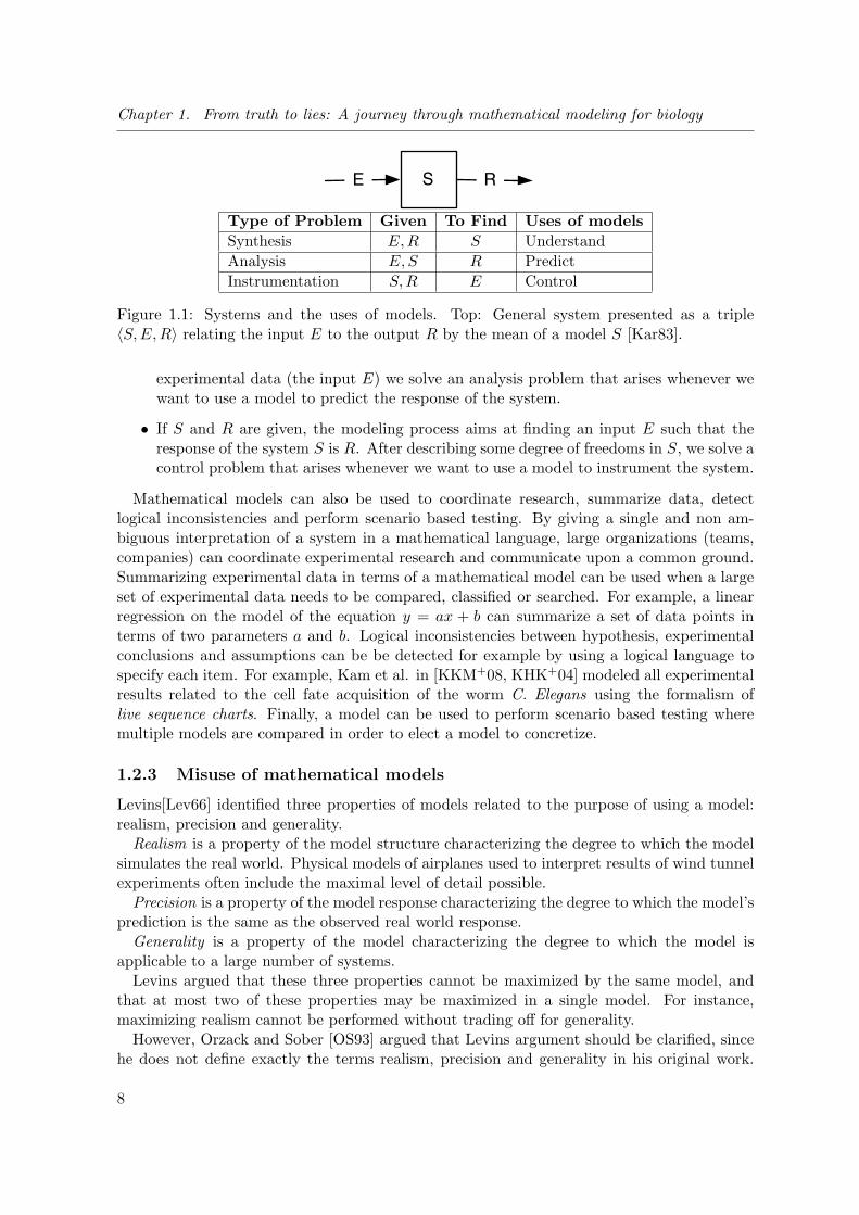
1.1 Systems and the uses of models. Top: General system presented as a triple〈S, E, R〉 relating the input E to the output R by the mean of a model S[Kar83]. . . . . . . . . . . . . . . . . . . . . . . . . . . . . . . . . . . . . . . . . 8
2.1 The structure of a simple two state automaton with labeled edges, displayedas a graph over Q. . . . . . . . . . . . . . . . . . . . . . . . . . . . . . . . . . . 17
2.2 Example of a non deterministic LTS. . . . . . . . . . . . . . . . . . . . . . . . 19
2.3 Semantics of a constraint automaton in terms of an LTS. . . . . . . . . . . . . 22
2.4 Lotka-Volterra dynamics for the rates k1 = 1, k2 = 0.1, k3 = 0.1 and initialconditions A(0) = k3/k2 + ǫ, B(0) = k1/k2 + ǫ as ǫ ∈ R ranges over [0, 1] bystep of 0.2. . . . . . . . . . . . . . . . . . . . . . . . . . . . . . . . . . . . . . . 35
2.5 Simulation of the LV system with extreme parameter value for k2. . . . . . . . 36
2.6 A single realization of a stochastic Lotka-Volterra system for the stochasticrate constants (1, 0.005, 0.6) and initial conditions (200, 100). This realizationis obtained with the function Step, implementing the Gillespie direct method. 37
3.1 Transition system of a bounded counter. . . . . . . . . . . . . . . . . . . . . . . 45
3.2 Illustration of connections between three BioRica nodes. Input variables i2 andi3 are made always equal to the output variable o1. Furthermore, in each ofthe nodes B1,B2,B3, an output variable value is dependent of the input variable. 51
5.1 BioRica software architecture. . . . . . . . . . . . . . . . . . . . . . . . . . . . . 121
6.1 A cell division cycle modeled as a transition system built with two variables“daughters” and “dead” respectively denoting the number of daughters and thestate of the cell (e.g. dead or alive). It is defined in BioRica by a node
containing those variables and the constrained events: dead = falsedivide−−−−→
daughters := daughters + 1; truedie−−→ dead := true. . . . . . . . . . . . . . . 137
6.2 Comparison of computationnal time needed to simulate a multi scale uncoupledsystem between GSL and BioRica. In BioRica, simulation were performed withand without memoisation. For example, simulation from 0 to 100 t.u. of thecoupled system with 124 ODEs (62 sub-populations) took 8.6s with the GSLwhile the equivalent system of 62 BioRica nodes took 0.7s without memoisationand 0.02s with memoisation. . . . . . . . . . . . . . . . . . . . . . . . . . . . . . 139
ix

List of Figures
6.3 Decomposition of a limit cycle of a two variables (x, y) system. By consideringthe sign and rank of the variables, we map an abstract value (here denotedby a formula) to each point of the trajectory. Boxes in the figure encompasssuccessive points that are mapped to the same abstract value. Successive pointsof the trajectory are collapsed whenever they have the same abstract value, thatis whenever they have the same sign and rank. This trajectory can thus beabstracted as a seven state QTS. . . . . . . . . . . . . . . . . . . . . . . . . . . 143
6.4 Example of piecewise linear approximation applied to two randomly generatednoisy time series. The first of the three successive plots represents the timeseries while the last two plots represent the result of the first two iterations ofthe PLA algorithm. After two iterations, the PLA algorithm selects two points(as well as the first and last point) that are considered as being representativeof the global shape of the time series. . . . . . . . . . . . . . . . . . . . . . . . . 148
6.5 Dynamic behavior of the cell cycle model for default parameter values. Left:an example of trajectory obtained by numerical integration of the Tyson cellcycle model [Tys91a]. Right: abstraction of this trajectory in terms of QTSby using the rank function as the abstraction function (transition labels areomitted). The total standard deviation of this QTS is 0.07. The states andtransitions highlighted by the circle correspond to stochastic transitions andrepresent numerical integration errors. . . . . . . . . . . . . . . . . . . . . . . . 149
6.6 Trajectory comparison for the Tyson cell cycle model. For 500 randomly sam-pled parameter spaces, we abstracted the simulated trajectory in terms of QTSby using the rank function. Trajectories were clustered in 9 bins by measuringthe Sorensen similarity index between each of the 500 QTS with the QTS ofthe figure 6.5. From each of the nine clusters, a representative trajectory isdepicted here together with its QTS and similarity value. These trajectoriesare sorted (column wise, increasing) by their similarity value. . . . . . . . . . . 150
6.7 Oscillation period for the MAPK cascade model. Left: contour plot repre-senting the period of oscillations. The bottom axis (resp. left axis) representsvalues of the k4 (resp. v5) parameter. The contour plot was built with 500simulations with random parameters. Regions with comparable periods arerepresented by a region with uniform color. Right: Two example trajectoriesexhibiting oscillations of minimal and maximal period A:1094 time units andB:2236 time units. . . . . . . . . . . . . . . . . . . . . . . . . . . . . . . . . . . 151
6.8 Example trajectories of the MAPK cascade exhibiting oscillating behaviorfound with a random sampling of ten parameters of the MAPK cascade model[Kho00]. On the right of each plot, the associated QTS reduced to its periodicform; under it, the period value with maximum likelihood. . . . . . . . . . . . . 151
6.9 ERK Crosstalk simulation results. From top left to bottom right, simulationresults are sorted by similarity with the non pathological case (reversible ac-tivation). The sampled value of v12 and the similarity index with the nonpathological case are under each plot. . . . . . . . . . . . . . . . . . . . . . . . 152
x

7.1 Three level hierarchical model, showing the discrete cell population and celldivision controllers, and the continuous single-cell model. This model generatespedigree trees during simulation, instantiating new single-cell models for eachcell division. Infinite width and depth are represented finitely by relaxing thetree constraints to permits loops from the leaves. These fixed points representsimmortal cells or immortals lineages. . . . . . . . . . . . . . . . . . . . . . . . 156
7.2 The numerical integrator advances between t (point 1) and the maximal step-size (2). The guards of events e1, e2 are satisfied. The regions where theseguards are satisfied are shaded. The firing time of e1 (3) is used to reset thesimulator after the discrete transition A (4). . . . . . . . . . . . . . . . . . . . . 158
7.3 Sample pedigree tree results for asymmetrical (Top) and symmetrical (Bot-tom) division strategies. Pedigree tree (Left) showing mother-daughter rela-tions; and simulation results (Right) showing single cell protein amounts overtime: normal proteins (blue), damaged proteins (pink), total proteins (dashed).For example, in the asymmetrical case with high damage, from time zero, theamount of normal proteins (blue) in the mother eventually cross the divisionthreshold at time approx. 0.15. At this time, the proteins repartition is ap-prox. 250 damaged proteins for 1750 total proteins. Once division is triggered,the progeny separates, and a new simulation is started for the mother (resp.the daughter) with initial normal proteins set at 1500 × 0.75 = 1125 (resp.1500 × 0.25 = 375) and damaged proteins set at 250 × 0.75 = 187.5 (resp.250× 0.25 = 62.5). Since in this case the mother accumulates damage over di-visions (compare damaged proteins amount between time 0.15 and 3.0), it willeventually reach a senescence point after 27 divisions. Comparison of its lifespan with the life span of each of its daughter and the life span of each daughterof its daughters (as tracked by the upper pedigree tree) shows a rejuvenationeffect. . . . . . . . . . . . . . . . . . . . . . . . . . . . . . . . . . . . . . . . . . 160
7.4 Sample parameter exploration result showing the high sensitivity and non lin-earity of the rejuvenation effect w.r.t. precise values of the damage rate k3.Only some ranges of the parameter value (approx. between 1.53 and 1.59) ex-hibits an increase of both the maximal and the mean fitness difference betweenevery mother and daughter of a population. Top: Estimation of the maximaland mean rejuvenation amount for damage rate ranging from 1.2 to 1.7 forthe asymmetrical and symmetrical case. The higher the values, the fitter somecells of the lineage are compared to their direct mother. Bottom: Close upof a lineage tree used to compute one point of the previous rejuvenation plot.Each node (yellow box) is labeled with an numeric id and the floating-pointfitness value of the cell, and each edge (white label) is labeled with the index ofthe daughter relatively to its mother and labeled with the difference of fitnessbetween daughter and mother. For such a given tree, we can compute the meanand max value of the edges, which is represented as one point on the rejuve-nation plot. The rejuvenation effect in young daughters of old mothers (rightblue colored branch) is consistent with the experimental results of [KJG94]. . 164
xi

List of Figures
7.5 Contour plot of mean of cell fitness from one generation level to the next(viability) over a pedigree tree, for a series of simulations in the symmetrycase. X axis: rate of damage of intact proteins (k3), Y axis: coeff. of retention(re). The lighter the color, the higher the mean, except for white regions,where the value is negative. This contour plot represents structured simulationresults for approx. 5, 120, 000 cells. . . . . . . . . . . . . . . . . . . . . . . . . 165
xii

General introduction
Over the last decade, availability of large-scale technologies and high-throughput experi-ments have resulted in an unprecedented accumulation of biological data. In its turn, thisaccumulation of data has increased the gap between human capacity to generate data andthat to analyze it. To complement usual “low-throughput” experiments, it is now possible tosequence complete genomes [HKKH91], to obtain gene expression data at the scale of an or-ganism [LW00] and to characterize the possible gene/protein and protein/protein interactions[LRR+02, UGC+00]. This progress in the measurements of rates of molecular mechanismsas well as the characterization of possible interactions between cellular processes implied aparadigm shift in life sciences. Indeed, the growing number of possible combinations of molec-ular interactions at the system scale results in a range of possible explanations for any observedbehavior that far exceeds the human capacity to evaluate them one by one [FMW+03]. Inthis context, the combination of mathematical biology and computational tools to analyzesuch systems (for example to a priori rule out some seemingly reasonable hypothesis) in silicois getting more and more accepted by the cell biologists and neurobiologists community.
Not only our knowledge of possible interactions is increasing, it is also now widely acceptedthat biological processes can not be seen statically. Models, in their broadest sense, havealways been used by biologists, e.g. when drawing a metabolic pathway or when consideringa graph of protein/protein interactions. However, we cannot deduce from such static repre-sentations alone the function of the process under consideration. For example, although thenutritional stress response of the model organism E.Coli and several metabolic pathways of theyeast Saccharomyces Cerevisiae have been characterized since decades, we yet to have a clearunderstanding of how these interactions result in biological functions [DHP04, BRDJ+05].Biologists emphasize now the need for mathematical and dynamic models to describe timedependent molecular processes. Indeed, living cells are inherently dynamic: cells grow, divide,communicate, move and respond to the evolution of their environment.
Let us consider two examples of biological dynamic phenomena, the electrical activity incells and the membrane transport mechanism.
Electrical activity in cells is one of the earliest dynamic behavior of cells that has beenstudied. Hodgkin and Huxley studied action potentials along a giant squid axon in 1939 andmodeled it in 1952 [HH52, HH39]. The electrical activity of the squid giant axon has beenstudied through the response of the axon to a small positive current. As the current propagatesalong the axonal membrane as a pulse, it results in a single spike of electrical activity (an actionpotential). Hodgkin and Huxley model is empirical, since they used experimental results thatwere suitable to be represented without consideration of any underlying physiological andcellular mechanisms. In fact, only thirty years after this seminal work, this observed behaviorwas explained by a “realistic cartoon” of ionic currents in cells [Hil01].
Another dynamic biological process of interest is the membrane transport mechanism. Theosmotic balance in cells is maintained by pumping Ca2+ and Na+ ions from the cell and K+
ions back into the cell. The maintenance of this balance is for example essential to give redcells their characteristic and functional shape.
xiii

The two previous biological processes are in fact coupled, and any system level analysisof membrane transport should account for the electrical activity in cells. In fact, Chay andKeizer have shown with a mathematical model in 1983 [CK83] that the increase of bloodglucose level induces insulin secretion, which in its turn induces regular bursts of electricalactivity in pancreatic cells. The action potentials occurring at the membrane of pancreaticcells are caused by rapid influx of Ca2+ and slower efflux of K+ that result in oscillations ofCa2+ concentration within the cytoplasm.
These two biological processes exhibit characteristics common to most biological processes:they are complex, can be seen at different levels of abstraction, and moreover they exhibita non linear response and their interactions are essential for higher-level behavior. In orderto study such complex networks of processes, the contribution of mathematical models andcomputing tools has been invaluable to understand their dynamics.
The combination of mathematical biology, experimental biology, biochemistry and com-puter science in order to unveil the behavior of biological systems lead to the “new” disciplineof Systems Biology. Systems biology is a field that aims at elucidating the relationshipsbetween biological components and how these interactions result in complex system-wise be-havior. The dogma at the base of Systems Biology is that due both to the presence of nonlinear responses and to multiple interactions between processes, the behavior of the wholesystem cannot be reduced to the behavior of its components. Furthermore, as the size andcomplexity of biological networks increase and will soon cross the threshold of manuallyunderstandable models [SRT06], one of the most important challenges for Systems Biologyis to develop computational tools that ease the manipulation and analysis of huge systems[SHK+06].
Strikingly, the same complexity also appeared during the last decade in the analysis ofengineered systems, and that in the both cases of software or hardware systems. Especially inthe case where the system is deemed as being critical, the vast amount of possible interactionsbetween disparate components imposed the need for formal methods to help the validation andanalysis phase. One striking similarity between Systems Biology and engineering is that bothfields are based on the compositional approach. Most biologists now agree that we will neverbe able to comprehend cellular networks in their whole, due to their “complexity” [SHK+06]and their growing size [SRT06]. As engineers have been faced with a similar limitation, theirsolution was to decompose large system into subsystems performing distinct, well defined andwell understood functions. The reason behind this approach is that a complex system can berationalized by considering it compositionally.
Composition in biological systems is however inherently different from the composition ofengineered systems. First, we do not know how to decompose a cellular network functionallyand thus what could be the definition of a biological “module”. Second, biological processescan operate at various time scales and be modeled at different levels of abstractions. Thus,a single modeling formalism to represent any biological module seems out of reach withinour current conceptions of Systems Biology. However, from the previous observations, anymodeling formalism adapted for Systems Biology should be hierarchical, compositional andshould allow for different modeling approaches.
Currently the most widely used modeling formalism is certainly that of systems of ordinarydifferential equations that represent the time dependent evolution of molecular concentrations.Under some conditions of homogeneity of the medium and of presence of chemical species athigh concentration, systems of ODE have been shown to produce extremely precise predic-tions, that have been validated experimentally (e.g see the evolution of a cell cycle model
xiv

[Tys91b, TKA+00, TCC+04]). Still, not only ODE models are flat, they are also completelydeterministic and thus can neither faithfully represent any stochastic behavior in cells, norcan they model adequately discrete timed behavior. For example, the model of [TCC+04]is a continuous differential equation model, built by accounting for the interactions betweenmolecular species that control the budding yeast cell cycle. Although the mechanisms of reg-ulation of the cell cycle are detailed, the authors completely abstract the cytokinesis processby representing it by a single discrete assignment that divides the mass of the cell by half,and that is triggered at a certain amount of time after a threshold is crossed. This exampleillustrates that although ODEs are powerful enough to concisely and adequately model nonlinear interactions between molecular species, they are not adequate to model more abstractprocesses for which little is known about the underlying mechanism or little is desired to berepresented in the model. When considering other type of modeling formalisms, although awide range of formalisms have been used (Petri Nets, constraint automata, differential equa-tions, stochastic pi-calculus), it is a humbling observation that the most widely used tools inthis technically sophisticated field remain for the modeling step PowerPoint and Excel, andfor model analysis step Matlab [KLH+07]. We propose to circumvent these limitations byconsidering multi-level and multi-formalism models.
Multi-level and multi-formalism models may be used when different levels of detail and ab-straction are possible within a hierarchical system [UDZ05]. That is, when a system accountsfor multiple molecular processes, for example happening at different time or concentrationscale, the level of details may be adapted in order to account for available knowledge andkinetics information. Existing simulation tools [TKHT04, BBHT06] can account for mod-els where molecular processes involving small concentrations are simulated with a variant ofStochastic Simulation Algorithm. In both cases, exact knowledge of the biochemical reactionsis required. In the case where biochemical information is missing (e.g. kinetic constants) someof the dynamics of a metabolic network can still be evaluated using pathway or genome scaleapproaches such as dynamic flux balance analysis [MED02] or structural analysis [SGSB06].
Accounting for unknown gene functions and/or interactions, is hard [vDMMO00]. We maythen consider that the qualitative behavior is essential in order to understand the system asa whole, while the accurate values of the kinetic parameters are of secondary importance.Indeed, the whole research community starts to accept this idea [SHK+06], which meansthat the time is ripe for moving from simulation only towards more symbolic model analysismethods. Behavioral analysis of models has been extensively studied in the context of formalverification of hardware and software systems. Here, models are usually non-deterministicautomata with variables over finite or infinite domains. Formal verification does not face the-oretical limitations (i.e. it is decidable) for finite-state models. However, this approach is inpractice limited by the so-called state explosion problem: the size of the model’s state space,that must be explored by the verification tool, is (at least) exponential in the number of vari-ables. The introduction of symbolic techniques [BCM+92] was a major breakthrough in thisfield, and nowadays models with a few hundreds of variables can be verified. Approximationtechniques have been developed in order to extend the reach of formal verification to largermodels, that can be finite-state (but with too many states) or infinite-state, such as automatawith (unbounded) integer variables. A wide class of techniques of approximation are basedon the notion of model abstraction. Model abstraction is based on the following observation:given a property under check, there are surely many details in the model that are not relevantto the property, and these details could therefore be abstracted away. Behavioral propertiesare preserved from an abstraction to its original model [DGG97], and abstractions can be
xv

computed automatically from the original model [GS97]. Model abstraction is an approxi-mation technique that have recently received a lot of attention since it permits automaticverification of software directly from the source code.
Another advantage of a multi-level hierarchical approach is clear when noticing how bio-logical processes take place at different time-scales. For example, transforming metabolitesis fast, while synthesizing an enzyme is slow. If modeled by ODEs, this multi-scale problemleads to the stiffness problem. It is the fast time-scaled reactions that are stable, but it isthe slow reactions that determine the trajectory of the system. If done naively, a simulationwill have to use extremely short time steps (which implies long simulation times) due to thefast time scales. Hierarchy can be seen as a way to overcome this issue. Indeed, simulation ofhierarchical systems can be done efficiently by having dedicated solvers for processes at dif-ferent granularities. Whenever a multi-component system is modeled, a semantics for modulecomposition has to be provided. In particular, a mathematical programming language knownas the stochastic pi-calculus allows the components of a biological system to be modeled in-dependently [Pri95]. In particular, large models can be constructed by composition of simplecomponents [BCP06]. The calculus also facilitates mathematical analysis of systems using arange of established techniques. Various stochastic simulators have been developed for thecalculus, in order to perform virtual experiments on biological system models.
Objectives and outline of this thesis
Due to the availability of more and more data and possible mechanisms to explain observedemergent behavior, Systems Biology approaches require compositional modeling tools able tocope with multiple formalisms and admitting efficient analysis tools. The challenges underthese requirements are both conceptual and computational. The conceptual difficulty is toprovide a modeling language that is compositional and expressive enough to reuse existingmodels. The computational difficulty is to analyze models described in this language, eitheranalytically / symbolically or by numerical simulation. The goal of this thesis is to provide anautomata based framework to describe and analyze stochastic processes in the field of systemsbiology.
The BioRica framework we present and analyze in this thesis can combine different for-malisms within a single framework and can efficiently simulate the resulting model. BioRicais a high-level modeling framework integrating discrete and continuous multi-scale dynamicswithin the same semantics domain, while offering an easy to use and computationally efficientnumerical simulator. It is based on a generic formalism that captures a range of discrete andcontinuous formalism and admits a precise operational semantics.
We first recall the background material and the domain of this work in the chapters Chap.1 and Chap. 2. The objectives of these two chapters is to define the methodology and thetools already available for the mathematical modeling of biological processes.
In the chapter Chap. 3, we define the BioRica language and its automata compositionalsemantics. BioRica is extension of the AltaRica specification able to specify non deterministicstochastic automata with timed transitions distributed arbitrarily. More precisely, we will takeas a starting point for BioRica the work done on the AltaRica specification language, andspecifically that on the AltaRica Dataflow subset([Rau02]), and we will extend its syntax andautomata semantics in order to account for probabilistic descriptions. We will then definecomposition operations in order to describe hierarchical systems with BioRica.
xvi

In the following chapter Chap. 4, we provide the semantics of BioRica programs in termsof stochastic transition systems and we establish gradually a symbolic computation schemeto compute the formula denoting the probability of a finite path with deadlines in such astochastic transition system. This analytical scheme is based on the computation of linearcombinations of random variables denoting timer values of discrete events. We also show thatby using this approach, computations with numerical values are only performed at the veryend if needed.
We then consider the problem of simulating a BioRica hierarchical system, and we providein chapter Chap. 5 the rules and algorithms to compile a BioRica system into a C++ programthat simulates the underlying stochastic process. Our approach is based on on the automaticgeneration of a set of C++ classes mapping the BioRica system hierarchy. We then adaptthe variable-time advance simulation schema to non deterministic hierarchical discrete eventsystems. The approach developed in this chapter were published in [SSN07].
In chapter 6, we provide abstraction based algorithms to build automata based representa-tion of transient behavior of continuous systems and show that high level emergent behaviorsuch as oscillations are preserved by our abstractions. In fact, given a range of possible qual-itative values represented as abstraction functions, we show how to compute from the timeseries generated by numerical integrators a stochastic transition system. This approach hasbeen presented and published in [SSN09].
Finally, we define and analyze in the chapter Chap. 7 a hierarchical and hybrid model ofa yeast cells population that explains the rejuvenation effect in symmetrically dividing yeastcultures by a retention factor. To this end, we describe how to incorporate continuous systemsinto a discrete BioRica system by using composition. From a differential continuous model,we describe a “hybrid system” accounting for cell division, and then build a population modelby parallel composition. We then interpret the predictions of this model with literature resultsconcerning damage segregation in asymmetrically and symmetrically dividing yeast cells. Theresults presented in this chapter were published in [CSS+08].
xvii

The Blind Men and the Elephant
It was six men of IndostanTo learning much inclined,Who went to see the Elephant(Though all of them were blind),That each by observationMight satisfy his mind.
The First approached the Elephant,And happening to fallAgainst his broad and sturdy side,At once began to bawl:“God bless me! but the ElephantIs very like a wall!”
The Second, feeling of the tusk,Cried, “Ho! what have we hereSo very round and smooth and sharp?To me tis mighty clearThis wonder of an ElephantIs very like a spear!”
The Third approached the animal,And happening to takeThe squirming trunk within his hands,Thus boldly up and spake:“I see,” quoth he, “the ElephantIs very like a snake!”
The Fourth reached out an eager hand,And felt about the knee.“What most this wondrous beast is likeIs mighty plain,” quoth he;“ Tis clear enough the ElephantIs very like a tree!”
The Fifth, who chanced to touch the ear,Said: “Een the blindest manCan tell what this resembles most;Deny the fact who canThis marvel of an ElephantIs very like a fan!”
The Sixth no sooner had begunAbout the beast to grope,Than, seizing on the swinging tailThat fell within his scope,“I see,” quoth he, “the ElephantIs very like a rope!”
And so these men of IndostanDisputed loud and long,Each in his own opinionExceeding stiff and strong,Though each was partly in the right,And all were in the wrong!
So oft in theologic wars,The disputants, I ween,Rail on in utter ignoranceOf what each other mean,And prate about an ElephantNot one of them has seen!
John Godfrey Saxe (1816–1887)
xviii

Part I
Background
1


Chapter 1
From truth to lies: A journeythrough mathematical modeling forbiology
The aim of this chapter is to show what is meant by a model, the nature and objectives ofthe modeling process and finally to discuss how models and especially mathematical modelscan be used within a scientific study in the case of biology. In particular, we will try toshow how different, competing models represented in different formalisms may be useful. Inessence, our objective is to show that new biological knowledge is “created” by the processof abduction, which is itself a logical fallacy. In order to reduce the impact of this fallacy,multiple hypothesis must be confronted on the basis of observations. Consequently, to bridgebetween observations and explanation or prediction, models are a fundamental (if not theonly) way to test a hypothesis.
1.1 What is modeling? What is a system?
Systems and models are primitive concepts (like those of a set or a structure) that are usedwith so many meanings and in so many domains that it might be impossible to give an exact,consensual definition. Although their understanding could thus be left to intuition alone, wenonetheless provide some (in our sense) representative definitions found in literature.
• A system is a regularly interacting or interdependent group of items forming an unifiedwhole (Webster).
• A system is a combination of components that act together to perform a function notpossible with any of the individual parts.(IEEE Standard dictionary of Electrical andElectronic terms).
• A model is a simplified description of a system or process, or even of another model. Themost common uses of models are to assist calculations, predictions and design choices.
• model (n): a miniature representation of something; a pattern of something to be made;an example for imitation or emulation; a description or analogy used to help visualizesomething (e.g., an atom) that cannot be directly observed; a system of postulates, data
3

Chapter 1. From truth to lies: A journey through mathematical modeling for biology
and inferences presented as a mathematical description of an entity or state of affairs[Dym04].
As it is usually pointed out for example in [Hae05], these definitions of model and systemsimply that virtually everything can be understood as a system and that models are presentin every facet of human activity.
Nevertheless, what can be observed from these different definitions is that a system is madeof interacting components, and that a model is an abstraction of a system. But more impor-tantly, these definitions suggest that modeling is a cognitive activity in which we think andmake models to describe how “real life” systems, processes or objects behave, by accountingfor their components; and that we use models to communicate a view of the world.
1.1.1 Scientific method and modeling: the principle of abduction
Scientific method may be rudimentarily outlined as opposing two a priori distinct worlds, a“real world” and a “conceptual world”. In the real world, we observe various phenomena andbehaviors, whether produced artifacts or natural. On the contrary, in the conceptual worldwe try to understand and explain what is going on in that real, external world.
Dym and Ivey [Dym04], describe the scientific method as a body of techniques existing in theconceptual world in order to reason about the real world. They identify three activities thattake place in the conceptual world when faced with a phenomenon: (1) we gather observations,(2) we analyze these observations by means of models, (3) we use the results of the analysisto describe precisely the phenomenon, to predict what would happen in a yet to be conductedexperience or to or explain the phenomenon. Let us discuss the mode of inference used inthis scientific method with holding to section Sec. 1.2 the details of these three possible usesof mathematical models. The base of the scientific method is the use of empirical data toform new body of knowledge. The mathematician Charles Sanders Peirce in “Deduction,Induction, and Hypothesis” (1878) (see [Nii99]) proposed different modes of inference properto the scientific method and that explain how empirical evidence can be used to form theories.Peirce compared deduction, induction and abduction. Consider the following syllogisms:
Rule All philosophers wear a toga,
Case These humans are philosophers,
Result Therefore these humans wear a toga.
The result is obtained via deduction. On the contrary, induction can be used to explainhow hypothesis and consequences are related.
Case A random sample of philosophers is selected.
Result All these philosophers wear a toga.
Rule All philosophers wear a toga.
However, experimental methods in a science like biology (and thus its use of models) relyon the use of abduction.
Rule All the philosophers wear a toga.
4

1.1. What is modeling? What is a system?
Result These humans wear a toga.
Case These humans are philosophers.
Indeed, the goal of abduction is to explain a “surprising” result. The surprising result is:seeing a group of humans wearing a toga. We must then seek an hypothesis that would makethis surprising result not surprising. It is true that if these humans are philosophers then theywould wear a toga, hence there is evidence to suspect that these humans are philosophers. Bythe observation of a surprising result, we seek a hypothesis that would explain this surprisingresult (and thus make it less surprising). Abduction thus seeks the most plausible hypothesisthat would explain a result, given accepted knowledge.
Note that abduction is a logical fallacy. Let a and b be two logical propositions. Deductionallows us to derive b as a consequence of a. Induction allows us to derive a ⇒ b by a set ofsamples of a and b. Abduction allow us to infer a from the observation of b. Abduction is thepost hoc ergo propter hoc fallacy (affirming the consequent) since we do not account for allthe possible explanations of b. In order to reduce the impact of this logical fallacy, we wouldhave to consider all the possible explanation for an observed phenomenon, which is clearlyimpossible.
1.1.2 From abduction to soundness: Chamberlain’s multiple hypothesistesting
Abduction is the only possible means to form a new body of knowledge by observation, butit is a mode of inference that is inherently wrong, since all the possible explanations of theobservation are not accounted for. However, by encompassing a wide range of possible expla-nations, one can hope to compare multiple explanations on the basis of empirical evidence.In order to cover and on the same time to limit the universe of explanations, we are forcedto simplify our view of reality and to keep only what we think is relevant for the observedphenomenon. In other words, we build models, and the possible explanations of an observedphenomenon are confronted by the use of multiple, competing models.
Thomas Chamberlain (1843-1928) advocated in a series of papers [Cha31](as cited by[And08]) that scientific investigation should focus on a set of alternative plausible scientifichypotheses that must be confronted. Each plausible hypothesis forms an explanation thatshould be evaluated with respect to its empirical support. In this sense, the core objective ofthe modeling process is to provide systematic and mathematical tools to aid in this evaluation.
As an example of a carefully shaped set of plausible hypotheses, Anderson [And08] high-lights the process and methodology Caley and Hone [CH02] followed while they were studyingbovine tuberculosis transmission in feral ferrets. Before performing any data collection, Caleyand Hone derived from literature review 20 hypotheses relating the instant of transmissionwith the age of the animal. As an example we provide here 5 of their hypotheses ([And08]):
• Transmission occurs until the 1.5 ∼ 2.0 months of age, via suckling, from mother tooffspring,
• Transmission occurs from the age of 10 months, via mating or fighting, during thebreeding season,
• Transmission occurs from the age of 2∼3 months, via routine social activities (e.g.sharing dens),
5

Chapter 1. From truth to lies: A journey through mathematical modeling for biology
• Transmission occurs from the age of 1.5 ∼ 2 months, via hunting,
• Transmission occurs from birth, via environmental contamination.
Each of the hypotheses targets at least two variables: the age of transmission and themedium of transmission; furthermore, these hypotheses are not mutually exclusive. Thus,evaluating and comparing each hypothesis with respect to empirical support should answerquestions about the“how”and“when”of contamination (i.e. “What is the size of the effect?”),which should be contrasted with the “what” of contamination (i.e. “Is there an effect?”).
From Anderson’s point of view, which follows closely Chamberlain’s and Francis Bacon’sapproach, the usual paradigm of investigation based on null hypothesis testing results mostof time (Anderson is in the field of ecology and population biology) in the rejection of afaulty and hardly plausible null hypothesis. Anderson concludes the tuberculosis example bychallenging the reader to devise a plausible null hypothesis and ironizes by suggesting thatH0 should be one of : “No transmission occurs”, “Transmission is random”, “Bears do no goin the woods”.
Given a phenomenon, multiple models must be assessed. Although Anderson’s work aimsexclusively at providing tools and strategies for confronting multiple hypotheses in the field ofstatistical modeling, our approach of systems modeling starts with the same principle: eachhypothesis should be supported by empirical data via the use of a model that is specific tothe hypothesis under scrutiny. Since we need multiple models, one of the objectives of thisthesis is to provide a modeling language that is able to describe models of different natureand to provide a mathematical interpretation of these models.
1.2 Utility of mathematical models
General definitions of models all agree on the fact that models represent reality with somerequired degree of approximation. Given that models are approximations and thus inherently“wrong”, why is this approximation required? What is exactly the purpose of the modelingactivity?
The general objective of the modeling process is to manage complexity. The overall com-plexity of technical systems is increasing. In several technical fields - telecommunication,information systems, logistics - the number of components involved in an object under designmakes it impossible to manage and predict the global effect of local decisions [Zim08]. Simi-larly, as our understanding of living systems increases, we witness an increase of complexityas we wish to understand how the possible interactions between thousands of molecules formthe basis of living organisms and their functional properties. In both of the technical andbiological fields, models offer a way to deal with this complexity. We will now consider in moredetail the attributes of this complexity in biology, then characterize the possible purposes ofmodels.
1.2.1 Models as means to deal with biological complexity
The nature of biological systems we wish to model in systems biology or in physiology arecharacterized by their complexity [CC08]. Yates [Yat78] identified five features of biologicalprocesses that give birth to their complexity: the number of components, their interactions,non linearity, asymmetry and nonholonomic constraints.
6

1.2. Utility of mathematical models
The number of components in the system is immediately related to its complexity. ButFlood et al. (1993) refined this point of view and have shown that it is from possible interac-tions between components that complexity emerges.
Nonlinear systems occur when one element of the system varies in a non linear manner withrespect to another. Non linearity is ubiquitous in biological processes [CC08]. However, froma modeling perspective, it can be reasonable to consider systems as being linear under someconditions.
Asymmetry in organisms is fairly usual and is a key property of cellular processes such acellular differentiation. Without the presence of asymmetry in one of the processes of growth,the successive divisions of a single cell would yield a population of identical cells and nospecialized organs would emerge.
Holonomic constraints are global constraints that are expressible as a function of the stateof the system and time. A system is said to be holonomic if all of its constraints are holo-nomic. Nonholonomy of biological processes appears whenever part of a system exhibits localregulation and control. At the unicellular level, consider for example glucose metabolismand cell cycle regulation of yeast cells. Even if these two processes are related (since theyare parts of the same system) and that they interact indirectly, there is no global constraintthat can express both processes, or equivalently, one of the processes as a function (in themathematical sense) of the other. Nonholonomy implies that some parts of a system exhibita high degree of freedom, and it is this absence of constraints that implies complexity. Thisimplies that the state of the system is not a function of the state of some of the parts of thesystem.
In other words, complexity arises in biology through the nature of interactions of the com-ponents of a system where non linear effects and control appear at multiple organizationallevels. As a consequence of this “real-life” complexity, it is often not possible to measure invivo with sufficient precision the values of the quantities of interest, since they may be at themolecular level. Often, only indirect measures about the quantities of interest may be ob-tained, implying at least the need for some model to be able to infer the value of the quantityof interest.
1.2.2 Use of mathematical models
Model[er]: A device for turning assumptions into conclusions Schimel (2002) (ascited by [Hae05])
The degree of detail that is incorporated in a model is determined by its purpose. Karplusin 1983 [Kar83] provided a conceptual framework to define the possible use of a mathematicalmodel. In Karplus’s framework, a model is a triple 〈S, E, R〉 where S is a black box systemwith an input E and an output response R (see figure Fig. 1.1)
Considering all the possible pairs of elements of 〈S, E, R〉 as problem statements, the useof the model is to characterize the third missing component.
• If E and R are given, the modeling process aims at determining the system S. Byinferring the system given its input and output, we solve a synthesis problem that ariseswhenever we want to use a model to understand a process.
• If E and S are given, the modeling process aims at characterizing the output responseR. By using the knowledge of the component (modeled as the system S) and available
7
Chapter 1. From truth to lies: A journey through mathematical modeling for biology
S RE
Type of Problem Given To Find Uses of models
Synthesis E,R S Understand
Analysis E,S R Predict
Instrumentation S, R E Control
Figure 1.1: Systems and the uses of models. Top: General system presented as a triple〈S, E, R〉 relating the input E to the output R by the mean of a model S [Kar83].
experimental data (the input E) we solve an analysis problem that arises whenever wewant to use a model to predict the response of the system.
• If S and R are given, the modeling process aims at finding an input E such that theresponse of the system S is R. After describing some degree of freedoms in S, we solve acontrol problem that arises whenever we want to use a model to instrument the system.
Mathematical models can also be used to coordinate research, summarize data, detectlogical inconsistencies and perform scenario based testing. By giving a single and non am-biguous interpretation of a system in a mathematical language, large organizations (teams,companies) can coordinate experimental research and communicate upon a common ground.Summarizing experimental data in terms of a mathematical model can be used when a largeset of experimental data needs to be compared, classified or searched. For example, a linearregression on the model of the equation y = ax + b can summarize a set of data points interms of two parameters a and b. Logical inconsistencies between hypothesis, experimentalconclusions and assumptions can be be detected for example by using a logical language tospecify each item. For example, Kam et al. in [KKM+08, KHK+04] modeled all experimentalresults related to the cell fate acquisition of the worm C. Elegans using the formalism oflive sequence charts. Finally, a model can be used to perform scenario based testing wheremultiple models are compared in order to elect a model to concretize.
1.2.3 Misuse of mathematical models
Levins[Lev66] identified three properties of models related to the purpose of using a model:realism, precision and generality.
Realism is a property of the model structure characterizing the degree to which the modelsimulates the real world. Physical models of airplanes used to interpret results of wind tunnelexperiments often include the maximal level of detail possible.
Precision is a property of the model response characterizing the degree to which the model’sprediction is the same as the observed real world response.
Generality is a property of the model characterizing the degree to which the model isapplicable to a large number of systems.
Levins argued that these three properties cannot be maximized by the same model, andthat at most two of these properties may be maximized in a single model. For instance,maximizing realism cannot be performed without trading off for generality.
However, Orzack and Sober [OS93] argued that Levins argument should be clarified, sincehe does not define exactly the terms realism, precision and generality in his original work.
8

1.3. How do we model?
Orzack and Sober thus refined Levins thesis and have shown that when a model A is a specialcase of another model A′, there is no trade-off between the three properties. They claimedthat for any model with n independent variables, we can add an additional variable and obtaina model that is more realistic, precise and general that the first one.
Models are tools used to solve a specific problem, and nothing in the model itself forbids aninappropriate application. Holling [Hol78] and Karplus [Kar77a, Kar77b, Kar83] especiallydiscussed the problem of the use of quantitative models and illustrated how highly precisemodels can be used in domains providing poor data or small understanding of the domain’sdynamics and mechanisms.
Karplus went further and identified domains in which the poor quality of the available dataand shallow understanding of the mechanisms led to inappropriate models. He positionedsocial science, economics and political science at the lower end of applicability of models. As anexample, Karplus cited Jay Forrester’s World Dynamics model which, more or less, accountedfor everything [For71]. Essentially, inappropriate use of models is one of the consequences ofthe possibility to simulate (or solve) quantitative models with an arbitrary number of digits,and that regardless of the accuracy of the premises used to build the model. Thus, althoughthe results are extremely precise with respect to the model (in the mathematical sense), thisprecision can be semantically skewed towards the precision of the model relative to the system,via an effect that Haefner [Hae05] qualified as “numbers which often acquire a reality of theirown”. Such semantic drift may be harmless, at best.
1.3 How do we model?
When using mathematics to model, two separate approaches to modeling are possible de-pending on the intended use of the model. These two approaches are data driven models andsystem oriented models.
When models are solely based on experimental data, we can apply a data driven modelingprocess that aims at building black-box models. In essence, data-driven models describe aninput output relationship between experimental data collected on the system. Data drivenmodels are mathematical descriptions of data, and have only an implicit correspondence withthe underlying biological process [CCB01].
The second modeling approach is system oriented modeling, with the goal to representthe underlying biological process explicitly, up to a level of approximation and resolutiondependent on the intended use of the model and on the availability of a priori knowledge andassumptions. Once the degree of approximation has been chosen, a mathematical formulationcan be built.
An important decision at the first step of the modeling process is to decide the level ofabstraction of the model. Deciding on the right level of abstraction is equivalent to decidingon what should be part of the model and what should be part of the environment. This steprequires careful thinking, since by identifying initially what should be accounted for in themodel, we also immediately delimit its application and purpose.
The result of this first step is a conceptual model. The conceptual model is usually notformalized and covers all the assumptions and approximations that are made before buildingthe mathematical model. In [CCB01], the authors identify three classes of possible approxi-mations: aggregation, abstraction and idealization. Approximation by aggregation considersa complex structure as an unified entity by lumping together its constituents. For exam-
9

Chapter 1. From truth to lies: A journey through mathematical modeling for biology
ple, the proteins in a mitochondria may be lumped together in five classes defined by theproteins’ function, or conversely they can be carefully modeled by accounting for the exactconcentration of each possible protein present in the mitochondria matrix. Approximationby abstraction matches a complex structure to its functional role. A mitochondria may beabstracted as an ATP producing unit. Approximation by idealization aims at simplifyingdynamics that are not considered as pertinent. For example, the response of a cell populationto oxidative stress implies the mitochondria of each cell. The response of the mitochondriamay be modeled either as being instantaneous and affecting all the mitochondria or modeledby accounting for the dynamics of the diffusion.
Once enough approximations are described in the conceptual model, the conceptual modelis translated into mathematical equations describing the relationships between the variablesof the model. A general hypothesis we have to apply to the system we wish to study by usingmathematical modeling is to consider that it is always in some state. A state of a modelfully describes the quantities we wish to measure with the model. This implies that the firststep when translating the conceptual model in mathematical equations is to define the set ofmeasurable variables that are chosen and associated with a given system.
Once state variables are defined, a general way to describe the behavior of a system is todescribe the structure of its state as well as how the system changes its state over time.
We will now introduce a simple classification based on the mathematical structure used torepresent the variables, the time and the dynamics.
1.3.1 Mathematical model formulation
A simple basis for the classification of models can rely on the structure of the underlyingmathematical theory used in the model. We consider that models can be:
• Process oriented when the mechanistic processes are explicited in the model. Otherwise,we say that the model is descriptive and phenomenological.
• Dynamic, when the state of the model evolves over time. Otherwise, we say that themodel is static.
• Continuous time, when the evolution over time is supported by a continuous variable.Otherwise, we say that the model is discrete time.
• Continuous, when the possible configurations of the model are real valued. Otherwise,we say that the model is discrete. For models over a discrete state space, we furtherdistinguish between finite and unbounded state space.
• Non deterministic, when the model is under-specified and allows for a set of possibleexecutions instead of a single execution. Otherwise, we say that the model is determin-istic.
• Stochastic, when an execution of a model depends on random variables. Otherwise wesay that the model is non random.
This classification of models serves as a methodological guideline during the modeling pro-cess.
We will review in the next chapter 2 instances of the previous classes and give an overviewof the analysis that can be performed on them.
10

1.3. How do we model?
In this thesis, we consider models that have a discrete state space, that evolve under con-tinuous time, by means of instantaneous transitions with random fluctuations. This choice isbacked up by the following reasons. The type of the state values and of passage of time is nota property of the system under consideration, but a property of the model we want to useto gain a better understanding of the system. This implies that this choice is independent ofthe question whether real systems are inherently continuous or not. When the state space isdiscrete and when time evolves continuously, the dynamic behavior of a model is described bytimed activities. The start of a timed activity is triggered by a precondition on the state of themodel, and their finishing events happen after some delay. Once the finishing event happens,the model evolves to its next state, where subsequent activities may start. By simply mod-eling the causality of activities within a model, one can use this model to answer qualitativequestions such as whether a given state of the model can ever be reached. However, whenquantitative properties are of interest, the model has to include additional information. As wesaw, the environment and the inner part of a model are subject to uncertainty. The processof modeling itself relies on abstracting some part of the system. This implies that whateverthe level of abstraction chosen for the model, there will always be some level of detail that isnot part of the model. This results in events that are unpredictable at this level, and that aretherefore modeled as being random. Note that this is independent of the question of whetherthere is true randomness or not. For example, conflicts between activities or events are asource of unpredictable behavior. Such conflicts can occur whenever two activities that arecompeting may alter the system’s state. Whenever the outcome of a conflict is not known atthe level of abstraction chosen for the model, we can still describe how the outcome should bedistributed by using probabilities. Another source of uncertainty in modeling arises when theexact time of an event is unknown. In this situation, we can consider the delay of an eventas a random variable following a given probability distribution function.
1.3.2 Hierarchical systems: from molecular to systems biology
Systems biology is a new field of biology that aims to develop a system-levelunderstanding of biological systems. [Kit01].
The objective of systems biology is to relate functional properties of whole systems withthe interactions of their constituents (Alberghina, 2005). The system’s behavior is oftenconsidered as an emerging behavior, that is a qualitative property that emerges from nonlinear interactions between components. This emergent behavior is often important for thesurvival of living organisms. The classical example is oscillation in networks of componentsthat would not oscillate on their own [GGH+01]. This implies that living systems shouldbe studied at multiple levels, between the molecular level and the systems level, and thatwe should explain the behavior of the whole system as emerging from the behavior of itsconstituents. According to [BBHW07], this leads to an apparent paradox inherent to systemsbiology: living systems are composed of nothing but molecules, but the functional propertiesof living systems cannot be understood by molecular biology alone. In essence, the paradoxcan be resolved by stressing the word “understood”. Bruggeman et al., 2002 advocate thatthere is no systematic choice between a purely reductionist approach (microscopic “nothingbut” statements) and an antireductionist approach (macroscopic “all or nothing”) approach,but rather a pragmatic choice of a middle position, with the aim to explain the system’sbehavior in terms of its functional organization.
11

Chapter 1. From truth to lies: A journey through mathematical modeling for biology
In order to explain the emerging behavior of complex living systems, hierarchical decomposi-tion is a modeling practice that decreases the complexity of the task. The simpler hierarchicalstructure of a system is based on the “part-of” relationship. For example, our perception ofthe human organism can be described in such terms: from genes, through cellular subsystems,cells, organelles and organs to the complete physiological organism [KS98]. In fact, this canbe said about systems in general, as hierarchy is deeply ingrained in the way we perceivenature and thus in the way we model it as a system:
Whether nature is truly organized hierarchically is moot. Men’s perception ofnature is hierarchical.[Web79]
By decomposing a system into its components, a top-down or bottom-up approach can beapplied to the modeling process, and this increases the “manageability” of a complex system[KE03]. However, as implied by the definition of the systems biology approach, the behavior ofthe whole system can not be expressed as a linear function of the behavior of its constituents,and thus a model of a system must account for non linear interactions.
Not only the complexity of the modeling task is decreased by decomposing a system, thisdecomposition is essential in order to exhibit regularity and patterns. When a system is de-composed in its parts (for a given relationship), it offers the possibility of detecting similaritiesbetween two different systems. As an example, the stress response circuitry of a prokaryoticorganism Escherichia Coli is present (albeit slightly modified) even in eukaryotic cells [Kit01].This implies that the model of the heat shock stress response in E.Coli may be reused to builda more complex machinery adapted to eukaryotic cells. By decomposing the E.Coli cell as asystem of interacting networks, some networks may be uncovered to be part of other systems.
Hierarchical modeling aims at decomposing a system into components that have enoughlocal regulation and control to be analyzed in isolation and such that they produce emergenteffects when analyzed within a system. As such, hierarchy is not a characteristic of a system,but a characteristic of the modeling process used to model the system. When a system isanalyzed, the objective is to explain the behavior at any level in terms of the level below, andhow this behavior explains the level above.[Web79]
1.3.3 Randomness in biology
The role of random fluctuations in biology can be seen in three conditions: limitations of themass action modeling assumption, accounting for uncertainties that concern the experimentaldata and finally as a necessary condition for explaining some biological patterns, like geneexpression or neuron firing.
In biochemical kinetics, the law of mass action states that the rate of a single reaction is pro-portional to the product of the concentrations of the reactants. This law is a key assumptionwhen deriving a set of differential equations from a network of biochemical reactions (see 2.7.2for an application and a discussion of this assumption). However, the stochastic approach tobiochemical kinetics is by far the methodology that is the most justified by statistical physicsconsiderations [Wil06]. Indeed, the conventional approach of modeling biochemical reactionnetworks by using continuous, deterministic rate equations can not be applied to systemswith multi-protein complexes or to systems where the dynamics depend on a species that ispresent in very low concentrations [Kit01, Gil77]. For example, behavior induced by signalingpathways is known to be sensitive to operations and reactions that happen for a small num-ber of molecules [GHLG03, Hal89]. For neutrophil signaling pathways, the study of Hallet
12

1.4. Model (in)validation for biology
[Hal89] showed that only the behavior of 200 K+ and Na+ ionic channels is responsible forthe intracellular concentration of Ca+.
Probabilistic models can be used in the modeling methodology and we will argue that thisis particularly useful in the case where a biochemical model covers a range of possible be-haviors and where little is known about the parameters used in the derivation of ODEs frombiochemical networks. The translation of a biochemical reaction network into a deterministiccontinuous equation requires at least the rate laws for all parameters. Once rate laws havebeen determined, the parametrized system obtained by the application of the mass action lawcan be studied, analyzed and solved. However, mass action kinetics fails to correctly capturethe saturation of enzymes, which is a common phenomenon. In order to account for enzymaticsaturation, more realistic kinetics can be applied (e.g. Michaelis Menten) which requires addi-tional parameters (e.g. the dissociation constant) and additional knowledge (functional formof the enzyme kinetics). But this approach is severely hampered by the the lack of availableenzymatic data, either concerning the value of the kinetic parameter or the functional formof the enzymatic rate equations. In the best case where both are available, parameter valuesmay have been obtained under different experimental conditions (temperature, physiologicalconditions) or for different strains or tissue type, which leads to thermodynamic errors whenused in the same model. To overcome this limitation, a probabilistic kinetics that accountsfor thermodynamic constraints has been proposed in [LK06b, LK06a]; [SGSB06] proposes astatistical exploration of the comprehensive parameter only requiring stoichiometric informa-tion. In both approaches, authors consider the parameters as being random variables andthey both provide techniques to characterize the plausible distribution of the parameters,thus leading to models that are not random, once initial conditions and parameter valueshave been selected by a randomized mechanism.
Finally, the behavior of a system can be explained by a high variability in its constituentsand this variability can be easily modeled by random variables. In the field of neurobi-ology, several studies outlined that the pattern of firing of individual nerve cells, and mostimportantly the range of possible patterns in a population of nerve cell, is explained by a prob-abilistic gating model of voltage-dependent ion channels[WRK00, SZ96]. In the case of blackbox models, data models using stochastic functions have been shown to be essential to cap-ture important unmeasurable disturbances in the field of neurophysiology [MN72]. Stochasticfluctuations are also abundant in gene regulation mechanisms, and McAdams [MA99] hasshown that some regulatory mechanisms do rely on variability induced by low intracellularconcentrations.
1.4 Model (in)validation for biology
Model validation is a problem specific process where we compare a set of competing modelby measuring their validity with respect to their intended purpose [CCB01] and deduce theirdomain of validity. In [CCB01], the author states that within a necessary domain of validity,the output of the model should “correspond sufficiently” to the experimental data, and hefurther states that “an acceptably small difference” is usual. This approach can be facilitatedfor parametric models by parameter estimation tools such as [ZK06]. Basically, given a set ofdata and a parametric model, tools can reduce the least square difference between a numericalsolution of an ODE and the initial data.
For models built using experimental data, Anderson [And08] emphasizes the need to define
13

Chapter 1. From truth to lies: A journey through mathematical modeling for biology
the impact of stochasticity in the initial data and thus the need to formalize any statisticalassumptions before comparing the output of the model with the experimental data. If thepurpose of the model is to have a perfect correspondence with the experimental data, itis always possible to perform a fit by using high order Fourier series or polynomial terms.Goodness of fit of n data points is always perfect when we use a polynomial of order n. Thisimplies that the objective of the modeling process is not to fit the data, but the informationin the data. Thus, defining for a specific modeling task what is the “signal” and what isthe “noise” should be equivalent to the definition of the model. The model is supposed toparsimoniously represent the information contained in the data.
In the case of Chamberlain’s approach, the goal is to build a one-to-one correspondencebetween the set of hypothesis and the set of competing models. We loosely used the notionof “a set of competing models” up to now and we now clarify what it means for two model tobe competing and link this notion with parametric models. In order to have two competingmodels, the notion of difference between models needs to be defined. As we saw in section Sec.1.3.1, different mathematical formalisms may underly the model and we can safely assumethat two models described in different formalisms are different. However, for models in thesame formalism the notion of different models can not be based on structural differences,but should be refined to account for parameters. Consider for example the logistic growthequation
dN/dt = rN(1−N/K)
As N decreases to 0, the limit of this model is the exponential growth equation
dN/dt = rN.
Although the exponential and logistic growth models are usually considered as being “differ-ent” since they exhibit different equations and structure, the exponential model is the limitcase of the logistic growth model. In other words if the parameter N is free, the logistic andexponential model may be equivalent. Thus, the non equivalence between two (parametric)models can only be evaluated once the parameters are set; the structure and equations ofthe models can not be used as a basis. Even in the case of more complex models, such asthe one obtained when deriving ODEs from a biochemical reaction network, the limit casewhen one of the parameter is 0 is a structurally different model. Thus, when building theset of competing models, each hypothesis should be mapped to a parametric model and itsparameter values. In other words, model identification and parameter estimation are exactlythe same process.
In the case where validation relies on experimental data, we are facing the task of selectingamong a set of competing models (or equivalently competing hypotheses), the “best model”.Anderson further recommends that one restate the problem as follows:
The issue becomes the evidence of each model, given the data.[...] So now we mayask if hypothesis C is 10 times as likely as hypothesis A ? (from [And08])
The theory presented in detail in [And08] defines exactly what is a good fitted model, giventhe data. Anderson provides statistical tools that can be used to rank the models by usingthe Kullback-Leibler information principle and its restatement by Akaike in terms entropymaximization principle. The beauty of Akaike’s information criterion is that it formally linksthe Kullback-Leibler principle, Boltzman entropy and Fischer maximum likelihood [And08].By using this criterion as a basis for model ranking and estimation of the quality of models,
14

1.5. Concluding remarks
Anderson provides a framework where quality of models is made relative to competing modelsand in which parsimony and goodness-of-fit are accounted for. Contrary to the approach ofLevins and of Orzack, in Anderson’s framework blindly adding free variables and parametersdoes not provide a better model.
In the case where validation can not be performed against experimental data, validationmust be made on the basis of qualitative results. The same biological system is described inmultiple formalisms. Indeed, as we saw in section Sec. 1.3.1 , there is a wealth of possibleformulations, and except when a formulation requires assumptions that are obviously falsefor the modeled system (such as the assumption of high number of reactants for the law ofmass action), the same system can be described by multiple models, each having their ownset of assumptions and specific abstractions.
Richard Levins [Lev66] suggested determining whether the predictions of the model resultfrom its specificities or from the details in the simplifying assumptions, by the use of a tech-nique he called robustness analysis. Robustness analysis is defined as searching for commonpredictions among multiple models of the same system [WR08]. In the case where the sameresult holds for each of these models, Levins qualifies the result as a robust theorem. Weisbergand Forber [WR08] applied this robustness analysis to the Lotka-Volterra model of prey pre-dation (that we study in more details in section Sec. 2.7.2). The author used four differentmodels: one is the original formulation in terms of ODEs, the three others being stochasticmodels based either on population dynamics, individual based dynamics, or density depen-dent individual based dynamics. They explored each model in order to validate the followingproperty
Ceteris paribus, if the abundance of predators is controlled mostly by the growthof the prey and the abundance of the prey controlled mostly by the death ofpredators, then a general biocide will increase the abundance of the prey anddecrease the abundance of predators.
The authors have shown that this property holds for all their possible model formulations,while other simpler properties don’t (stating e.g. that the average number of predators andprey corresponds to a stable equilibrium point). The authors refer to [CD89] for an illustrationof a “real life” application of this principle: by using the DDT pesticide as a treatment againstIcerya purchasi, a scale insect, orchardists in fact have aggravated the pest invasion since theinsecticide has also killed the pest’s main predator.
1.5 Concluding remarks
In this chapter we have defined the terms and concepts that underly the work done duringthis thesis. We gave an overview of how the modeling process may fit in the scientific method,why models are required for biological sciences, what are the inherent limitations of models,and provided some guidelines for the modeling process and for model validation.
In summary, mathematical models are abstractions that depict reality. When the experi-mental data is present, the use of mathematical models can be seen as that of maximizingthe information that can be gained by measurements, by a formalization of the impact ofnoise and random fluctuations. When measures of quantities of interests are not available,mathematical models can be used to infer plausible values from the experimental data. Inthe extreme case where experimental data is not available, mathematical models may still beused to exhibit general principles about the behavior of complex systems.
15

Chapter 1. From truth to lies: A journey through mathematical modeling for biology
In any case, models are means to increase our understanding of complex systems, by therelying on approximation. In this sense, models are never “true”, they always reflect only theparts of reality that we conceptually think are relevant to explain the observed behavior. Tohave a true model, such as a perfect model for the whole cell, would require an extraordinaryquantity of experimental data to estimate its parameters, and an extraordinary amount oftime to understand and interpret its output behavior.
In order to build hierarchical systems, models should not be reused directly without inter-pretation or further approximations. Model reuse is a major research effort in modeling andsimulation [UDLK05]. In the field of systems biology, the complexity of the modeling processmakes reuse of existing models extremely appealing. The challenges currently faced by thesystems biology community include the interpretation of such composed models, the technicalinteroperability of the corresponding simulation systems, and modeling and simulation thataccounts for multi-formalisms and hierarchical systems . This problem has been identified as agrand challenge in the systems biology community[SHK+06]. As illustrated by the BioModelsdatabase [LNBB+06], the output of the modeling process is often reduced to its mathematicalartifact, namely the model itself, without all the assumptions, experimental data, conceptualconsiderations and validation methods that have been used to elect a candidate model as the“true” model. Even if technical and mathematical tools provide a framework where modelcomposition is possible (and this thesis indeed provides one of them), a complex model builtby reusing existing models that have been obtained with different assumptions seems hardlyplausible.
16

Chapter 2
Modeling formalisms
The aim of this chapter is to present the preliminary notions and modeling formalisms usedthorough this thesis. After introducing the discrete model of finite state automata and oftransition systems, we recall the definitions of constraints automata and their extension thatserve as a basis for the semantics of the AltaRica formalism. Afterwards, we recall somedefinition of probability theory and present two widely used stochastic processes class: discretetime discrete state Markov chain and continuous time discrete state Markov chains. We thenfinish this preliminary section by presenting the notion of discrete event systems and byintroducing model formalisms widely used in mathematical biology.
2.1 Discrete and finite models
2.1.1 Finite Automata, transition systems
The first model of behavior we present is the model of an automaton, also called a finite statemachine. An automaton is a directed graph with labeled edges. Each node of the graph ismeant to represent a possible state of the system, while edges represent transitions that arediscrete steps that can change the state of the system. A transition has a source and a targetstate. The source state represents the state before “executing” (or “firing”) the transition, andthe target state is the state reached after executing the transition. A self explaining exampleis given in Fig. 2.1.
In[17]:= Q= 8" Light off ", " Light on " <;S = 8" switch " <;rel = 88" Light off " ® " Light on ", " switch " <,8" Light on " ® " Light off ", " switch " <<;
GraphPlot @rel, DirectedEdges ® True, VertexLabeling ® True D
Out[20]=
switch
switch
Light offLight on
Figure 2.1: The structure of a simple two state automaton with labeled edges, displayed as agraph over Q.
Automata are probably the most used formalism to model the behavior of discrete sys-
17

Chapter 2. Modeling formalisms
tems. See, for example, the automata representation of programming languages semantics[Plo81, Win93], and model checking [QS82, CE81]. By using automata as the mathematicalrepresentation of the possible behaviors of a system, model checking algorithms and tech-niques based on relations over automata such as language inclusion [HMU06] or bisimulation[Mil82] can be used to validate the compliance of a system with respect to a set of behaviorsdescribed using an appropriate logic (e.g. LTL, CTL [CE81, Pnu77]).
While the structure of an automaton is always described as a graph structure, automataare usually decorated graphs, giving rise to many different subclasses. To begin with, we recallthe definition of labeled transition systems that are automata whose edges are labelled withevents.
Definition 2.1 (Labeled transition system). A finite labeled transition system (LTS) isa triple 〈Q,Σ,→〉 where
• Q is a finite set of states q, q′, q0, . . . , qn called the state space,
• Σ is a finite alphabet of events e, e0, . . . , em,
• →⊆ (Q× Σ×Q) is a (finite) set of labeled transitions.
To simplify the notations, a transition (q, e, q′) ∈→ is written qe−→ q′. For a given LTS
L = 〈Q,Σ,→〉, we write qe−→q′ if (q, e, q′) /∈→.
The LTS structure 〈Q,Σ,→〉 from the example in figure Fig.2.1 is Q = “Light on”,“Light off” ,Σ =switch with the transition relation defined by
→= (“Light on”,“switch”,“Light off”), (“Light off”,“switch”,“Light on”) .
In order to introduce some terminology, let us consider the example of figure Fig. 2.2.In the LTS defined in Fig. 2.2, it should be noted that not all events are enabled in
every state. For example, there is no outgoing transition from the state y labeled with theevent c. We say that the event c is inactive in y. Furthermore, note that in state x, thereare two outgoing transitions labeled with the same event a, we say that this state is nondeterministic, in the sense that whenever the event a happens, the model does not providesufficient information to decide on a single successor state, and thus all the possible successorscan potentially be reached by a single transition.
2.1.2 Composition of labeled transition systems
Labeled transition systems can be composed by using the synchronized product of Arnold-Nivat [Arn94, Arn92]. Let Si be a set of LTS with Si = 〈Qi, Σi,→i〉 and consider asynchronization constraint I ⊆ ∏i Σi. The synchronized product of the Si with respect tothe synchronization constraint I is the LTS S = 〈Q,Σ,→〉 where Q =
∏i Qi, Σ =
∏i Σi, and
where
(s1, . . . , sn)(e1,...,en)−−−−−−→ (s′1, . . . , s
′n)⇔ (e1, . . . , en) ∈ I, si
ei→i s′i,∀i, 1 ≤ i ≤ n.
In the case where I =∏
i Σi, the synchronized product is equivalent to the free product.
18

2.1. Discrete and finite models
In[25]:= Q= 8x, y, z<;S = 8a, b, c<;rel = 88x ® y, c<, 8x ® z, a<, 8z ® z, b<, 8z ® y, a<, 8z ® y, c<, 8y ® y, b<,8y ® x, a<, 8x ® y, a<<;
GraphPlot @rel, DirectedEdges ® True, VertexLabeling ® True D
Out[28]=
c a a
b
a
b
a
c
x
y z
Figure 2.2: Example of a non deterministic LTS.
2.1.3 Semantics
An important notion we use in this manuscript is the notion of semantics associated with aclass of models. We (loosely) define a semantics as a function mapping a model in a givenmodeling formalism to a model in another formalism (in this we follow [NN92]). For example,for the LTS we can provide a semantics in terms of languages. A language over an alphabet Σis a set of words that are finite sequences (ei)i≤n where ei ∈ Σ. Given an LTS L = 〈Q,Σ,→〉,the semantics of L in terms of languages is the set of words denoted JLK such that for any
word (ei)i≤n ∈ JLK, there exists a sequence of states (qi)i≤n+1 such that qiei−→ qi+1 for all
i ≤ n. Note that the semantics of a structured object such as an LTS is given in terms of lessstructured objects: sets generated by application of the binary operation of concatenation.In this sense, this implies that all the semantics defined in this thesis are not necessarilysurjective. For instance, for the semantics of an LTS in terms of languages, it is known thatthere is no finite transition system or finite automaton whose semantics is language anbn forsome integer n [HMU06]. In other words, there exist (in fact an infinite number of ) languagesthat do not represent the semantics of any LTS.
2.1.4 Variables, Logic
The core limitation of using LTS to model a dynamic system is that the state space and thetransition relation are explicit. In order to ease the description of complex systems with LTS,we can use a higher level (i.e. more structured) formalism the semantics of which will begiven in terms of LTS. We will introduce the notion of constraint automata [BR94], that areautomata with an implicit transition relation and state space, that manipulate variables bymeans of assignments whenever the current valuation of the automaton satisfies a constraint.In order to formally define this object we first need a logical language to define the notions
19

Chapter 2. Modeling formalisms
of variable, valuation and constraint. We only give here an overview of the logic, for a morethorough treatment, see [LC03, HR04].
A constraint automaton manipulates variables that are defined over a finite domain limitingthe possible valuations. More formally, we have domains and variables as provided in thefollowing definition.
Definition 2.2 (Domains and variables). The domains, variables, domain of variablesand valuations are defined as follows.
• Z = a, b, c, . . . is a finite set called the domain the elements of which are calledconstants. We consider for constraint automata that Z is a finite subset of Z.
• X = x, y, z, . . . is a finite set of variables.
• An application dom : X → P(Z), such that for any x in X, dom(x) 6= ∅. The applicationdom(x) is called the domain of the variable x, i.e. this is the set of possible values forthe variable x.
• The set extension of dom, i.e. for any Y ⊆ X, dom(Y ) =∏
y∈Y
dom(y).
• A valuation v is an application X → Z that assigns a variable x to its value v(x) ∈dom(x).
• For any variable x ∈ X, for any valuation v, for any value a in dom(x), we define v[a/x]to be an updated valuation of v where v[a/x](x) = a and where v[a/x](y) = v(y) ifx 6= y.
The expressions and formulas used in constraint automata are terms and formulas of aquantifier free first order language. The elements of Z are the constants of our languageand these elements are considered as being nullary functions. Let F be a set of functionscontaining at least Z, the terms over F are defined inductively with the following BackusNormal Form grammar:
t ::= x | c | f(t, . . . , t)
where x ranges over the set of variables X, c over nullary function symbols in F , and f overthe elements of F with arity n > 0.
Let P be a set of predicate symbols, the formulas of a constraint automaton are defined bythe following Backus Normal Form grammar:
φ ::= 1 | 0 | p(t1, . . . , tn) | ¬φ | φ ∧ φ | φ ∨ φ | φ⇒ φ
where 1 and 0 are symbols denoting the usual boolean constants true and false, p ∈ P is apredicate symbol of arity n ≥ 1 and ti are terms over the functions F . Let Y ⊆ X be a setof variables, we will denote by T Y and FY the set of terms and formulas built with variablesin Y . In the case where Y = X, we omit the superscript and simply write T and F .
We will denote by vars(φ) or vars(t) the set of variables occurring in the formula φ or in theterm t.1 Any formula φ(x, y, z, . . . ) is intended to be interpreted with respect to the finite setof variables X. Thus, the semantics JφK of a formula φ is a subset of dom(X). We define the
1For first order language with quantifiers, this is usually the set of free variables occurring in a formula.
20

2.2. Constraint automata
semantics of the boolean constants 1 and 0 by J1K = dom(X) and J0K = ∅. Finally, given aformula φ, a variable x and a term t, we define φ[t/x] to be the formula obtained by replacingeach occurrence of the variable x with t. In the following, we fix the functions and predicatesto be F = +,−, ∗, / and P = =, <,>,≤,≥.
Example 2.1. Suppose n, f and g are function symbols respectively nullary, unary andbinary. Then g(f(n), n) and f(g(n, f(n))) are terms, but not g(n) (it violates the arity).Suppose 0, 1, . . . are nullary, s is unary and +,− are binary. Then −(2,+(s(x), y)) is a term.Usually, binary symbols are written in the infix manner rather than in the prefix manner;thus, the term is written 2 − (s(x) + y). For a set of variables X = x, y, z with domainsZ = dom(x) = dom(y) = dom(z) = 0, . . . , 10, the formula φ(x, y, z) = x+ y +3 ≤ 4 admitsthe semantics JφK = 〈0, 0, Z〉∪〈0, 1, Z〉∪〈1, 0, Z〉∪〈1, 1, Z〉 where 〈a, b, Z〉 = 〈a, b, c〉 | c ∈ Z.
2.2 Constraint automata
A constraint automaton ([BR94] as cited by [Pag04] and [FP93]) is defined as follows.
Definition 2.3 (Constraint automaton, not interfaced version). A constraint automa-ton is a tuple A = 〈S, Σ, A,M〉 where
• S is a set of variables called state variables,
• Σ is a finite alphabet,
• A ∈ FS is a formula over variables called the global assertion,
• M ⊂ F × Σ× (S → T ) is a set of macro transitions 〈g, e, a〉 where:
– g ∈ FS is called the guard,
– e ∈ Σ is the label of the event representing the transition,
– a : S → T S maps every state variable to a term denoting its value after thetransition. This mapping is called the assignment of the transition. Note that thisapplication is complete, therefore every state variable is related to a term, that canbe reduced to the variable itself if it is not affected by the transition.
In the next section we will formally define the semantics of a variant of constraint au-tomata called interfaced constraint automata. Since we reuse most of the construction ofthe semantics of constraint automata, here we only provide an intuition of their LTS seman-tics. Consider a constraint automaton A = 〈S, Σ, A,M〉 where S = x, F = ∅, Σ = e,A = 1, M = (x ≤ 3, e, x→ x + 1), (x > 3, e, x→ x + 2), we will manually build the LTSJAK = 〈Q,Σ,→〉. The set Q is the domain of the variables, that is Q = dom(x) that we setto Q = 1, 2, . . . , 6. An element of Q is called a configuration in order to distinguish easilybetween a state and state variables. Consider the configuration 〈3〉 corresponding to the val-uation x : 3. The set of macro-transitions that have a guard satisfied by this configuration is(x ≤ 3, e, x → x + 1). Therefore, in the underlying LTS, we have the transition 〈3〉 e−→ 〈4〉.The configuration 〈5〉 of the LTS corresponds to the valuation x : 5, for this valuation, theset of macro-transitions that have a guard satisfied is (x ≥ 3, e, x→ x + 2), however theassignment x→ x + 2 is forbidden since it will cause an overflow for the variable x. The setof transitions of this LTS is depicted in figure Fig. 2.3.
21

Chapter 2. Modeling formalisms
In[79]:= Q= Range@6D;Union @
If @ð £ 3 ì ð + 1 £ 6,8ð ® ð + 1, " e" <D & Q,
If @ð ³ 3 ì ð + 2 £ 6,8ð ® ð + 2, " e" <D & Q
D@@2 ;; DDGraphPlot @%, VertexLabeling ® True, DirectedEdges ® True,
SelfLoopStyle ® NoneD
Out[80]= 881 ® 2, e<, 82 ® 3, e<, 83 ® 4, e<, 83 ® 5, e<, 84 ® 6, e<<
Out[81]=
e
e
e
e
e
1
2
3
4
5
6
Figure 2.3: Semantics of a constraint automaton in terms of an LTS.
2.3 The AltaRica formalism
Although the constraint automata described in the previous section provide a more concisedescription of systems than LTS by means of variables and arithmetic operations, they arenot a priori adapted to describe systems of interacting components. The AltaRica formalism[AGPR00, Poi00] has been designed to describe the possible interactions between components.AltaRica is a hierarchical specification language based on interfaced constraint automata andin which compositions are performed by the synchronized product of interfaced constraintautomata.
An interfaced constraint automaton, also called a component, is defined as follows.
Definition 2.4 (Constraint automaton, interfaced version). An interfaced constraintautomaton is a tuple A = 〈S, F, Σ, A,M〉 where
• S is a set of variables called state variables,
• F is a set of variables called flow variables,
• Σ is a finite alphabet containing at least the letter ǫ; the letter ǫ denotes the label ofthe invisible event,
• A ∈ FS∪F is a formula over variables called the global assertion,
22

2.3. The AltaRica formalism
• M ⊂ F × Σ× (S → T ) is a set of macro transitions 〈g, e, a〉 where:
– g ∈ FS∪F is called the guard,
– e ∈ Σ is the label of the event representing the transition,
– a : S → T S∪F maps every state variable to a term denoting its value after thetransition. This mapping is called the assignment of the transition. Note that thisapplication is complete, therefore every state variable is related to a term, that canbe reduced to the variable itself if it is not affected by the transition.
The macro transitions M always contain the macro transition 〈1, ǫ, Id〉 where Id is theidentity function.
The main differences between the interfaced and not interfaced version of a constraintautomaton are the set of flow variables and the presence of a specific event ǫ denoting aninvisible event. These two additions are the basis for hierarchical composition, and this isillustrated in the semantics of a constraint automaton is terms of LTS. This semantics isdefined as follows.
Definition 2.5 (Semantics of a constraint automaton in terms of LTS [Poi00] ). Thesemantics of a constraint automata A = 〈S, F, Σ, A,M〉 is the LTS JAK = 〈Q,Σ,→〉 whereQ = (s, f) ∈ dom(S ∪ F ) | (s, f) ∈ JAK and where (s, f)
e−→ (s′, f ′) if (s, f, e, s′) ∈M and if(s′, f ′) ∈ JAK.
For a component in isolation, the other components in the system are abstracted by flowvariables (representing variables visible by many components) and by the epsilon invisibleevent (representing external transitions updating the flow variable). This is implied by theLTS semantics since after each transition of a component, the flow variables are allowed to takeany value within their domain, as long as the global assertion is respected. For a componentin isolation, each transition triggers non deterministically an update of the valuation of flowvariables. In the case where the transition of a component is guarded by a flow variable,the semantics in terms of LTS allows the component to make a empty transition 1
ǫ−→ Id inorder to always allow an update of the value of this flow variable. By this construction, thepossible behavior of a component with flow variables uses non determinism to encompass allthe possible behaviors of other components, even if they are not yet specified.
Flow variables are not assigned but constrained via the global assertion of a component.According to the definition of macro-transitions, it is not possible to assign a value to a flowvariable as a result of a transition. In fact, the only possible way to “assign” a value to a flowvariable is to constrain it by the use of the global assertion. For example, in a componentwith a state variable x and a flow variable f , the flow variable can be constrained to alwayshave f = x + 1.
Hierarchical models in AltaRica are defined in terms of AltaRica nodes that are structuresthat contain other AltaRica nodes or components. An AltaRica node specifies synchronizationconstraints that are used when giving its semantics in terms of LTS. Basically, the semanticsof an AltaRica node is defined as the synchronized product of the LTS that are the semanticsof the components of the AltaRica node. The synchronization constraints are used to modelevents that should always occur simultaneously in the hierarchical model, while a globalassertion is used to represent how flow variables should be coordinated in the hierarchy. Wewill come back to these notions in the next chapter, when we define the syntax and semanticsof a BioRica node.
23

Chapter 2. Modeling formalisms
The AltaRica formalism also accounts for priorities between events and for scoping of eventand flow variable visibility in the hierarchy. Priorities are a partial order < over eventsspecifying that if events e and e′ are enabled in the same state and if e < e′, then only thetransitions labeled with e′ are effective. Events and flow variables can be scoped. This permitsone to restrict an event synchronizability to its parent node or to restrict the visibility of aflow variable to itself.
2.4 Probabilities and measure
This section presents some notions of probabilities which are necessary for this thesis. Thefollowing brief introduction is based on a synthesis of [Haa02], [FF98],[Zim08],[Gut05] and[F+57].
Let Ω be a set, called the sample space, that represents the possible outcome of a randomprobabilistic experiment. A subset A ⊆ Ω is called a (probabilistic) event. An event A occurswhenever the outcome of a probabilistic experiment is in A. In order to model the set ofpossible events, a σ-field (also called a σ-algebra) F is associated with Ω. The σ-field F is acollection of events such that
• ∅, ω ∈ F ,
• for a subset A ⊆ Ω, A ∈ F , we have Ac ∈ F , where Ac = Ω−A = ω ∈ Ω | ω /∈ A,
•(⋃+∞
i=1 Ai
)∈ F whenever Ai ∈ F for all i ≥ 1.
The σ−field generated by a collection A ⊆ F is the smallest σ-field containing A, it is theintersection of all σ-fields containing A.
We can then define a probability measure P over F as a non negative real-valued functionsuch that
• P (∅) = 0,
• P (Ω) = 1,
• P (⋃
Ai) =∑
P (Ai),
whenever (Ai) is a (finite or countably infinite) collection of disjoint sets in F . Then weimmediately have for any A, B ∈ F ,
• 0 ≤ P (A) ≤ 1,
• P (Ac) = 1− P (A),
• A ⊆ B implies P (A) ≤ P (B).
In particular, if there exists a countable set A ∈ F such that P (A) = 1 then P is said tobe a discrete probability measure and 〈Σ,F , P 〉 is called a discrete probability space.
The support set [Rud74] of a probability measure is the smallest subset of the sample spacewhose measure is 1. Formally, the support set of f is the set
supp(f) = Ω−⋃A ∈ F | A is open and P (A) = 0 .
24

2.4. Probabilities and measure
Definition 2.6 (Measurable and probability space). The pair 〈Ω,F〉 is called a mea-surable space, the triple 〈Ω,F , P 〉 is called a probability space.
Definition 2.7 (Measurable functions). Let 〈Ω,F〉 and 〈Ω′,F ′〉 be two measurable spaces,a function f : Ω→ Ω′ is said to be measurable if the set f−1(A) = a | f(a) ∈ A is in F , forany set A ∈ F .
In order to push forward a measure P , we have the following result.
Proposition 2.1. If f is a measurable function as before and if 〈Ω,F , P 〉 is a probabilityspace, then P f−1 is a probability measure on 〈Ω′,F ′〉 and the triple
⟨Ω′,F ′, P f−1
⟩is a
probability space.
For an event B such that P (B) > 0, the probability of an event A conditional on B, denotedP (A | B) is defined as
P (A | B) =P (A ∩B)
P (B).
The mapping PB from Fto [0, 1] with PB(A) = P (A | B) defines a probability measure PB
on F .
Definition 2.8 (Countable partition). A collection of events (Bi)i∈I is called a (countable)partition of Ω if
1. I is countable,
2. i 6= j implies that Bi ∪Bj = ∅,
3. P (Bi) 6= 0 for all i ∈ I,
4. Ω =⋃
i∈I Bi.
Theorem 2.2 (Law of total probability). Let (Bi) be a partition of Ω and A ∈ F be anevent, we have
P (A) =∑
i∈I
P (A | Bi)P (Bi).
We say that the events A, B are independent if P (A ∩ B) = P (A)P (B). We say that theevents A0, . . . , An are mutually independent if
P (Ai1 ∩ . . . Aik) = P (Ai1)× . . .× P (Aik)
for 2 ≤ k ≤ n and for 0 ≤ i1 ≤ i2 ≤ · · · ≤ ik ≤ n.
2.4.1 General measures and Borel spaces
For a σ-field F , a non negative real valued function µ over F is a general measure if µ is aprobability measure without the constraint that µ(ω) = 1. If µ(A) > 0 for some A ∈ F , µ issaid to be non trivial.
Let ℜ be the σ-field generated by the set of open intervals of the real line (a, b), the elementsof ℜ are called the Borel sets. Then let µ be the unique measure on the measurable space〈R,ℜ〉 such that µ((a, b)) = b−a for each interval (a, b). This measure µ is called the Lebesguemeasure.
25

Chapter 2. Modeling formalisms
Let Rn be the n-dimensional real space, and let ℜn be the σ-field generated by the class of
rectangle sets of the form (a1, b1) × . . .× (an, bn), then the n-dimensional Lebesgue measureµn is the unique measure such that
µn(A) =n∏
i=1
(bi − ai).
In this thesis, we consider only probability spaces that are either countable or isomorphicto some Borel space defined on a real hyperspace.
2.4.2 Random variables and Probability distribution functions
Definition 2.9 (Random variable). A random variable (r.v.) X on a probability space〈Ω,F , P 〉 is a real-valued function defined on Ω and measurable with respect to F , that isω ∈ Ω | X(ω) ≤ x ∈ F for x ∈ R.
The previous definition is usually generalized for n dimensional r.v. that are measurablefunctions from a probability space to 〈Rn,ℜn〉.
The σ-field σ 〈X〉 generated by a r.v. X is the smallest σ-field containing all sets of theform ω | X(ω) ≤ x. We always have σ 〈X〉 ⊆ F .
Note that in the definition of a random variable, the probability measure of the initialprobability space is not used at all. In fact, we can dispose completely of this initial probabilityspace and only consider the probability measure induced by a random variable, as stated bythe following proposition.
Proposition 2.3. Let X from 〈Ω,F , P 〉 to 〈Rn,ℜn〉 be a r.v., then the function PX from ℜn
to [0, 1] defined byPX(B) = P (X−1(B))
for any borel set B is a probability measure on 〈Rn,ℜn〉.
The distribution of a r.v. X is the probability measure µX defined on the measurable space〈R,ℜ〉 such that µX(A) = P (ω ∈ Ω | X(ω) ∈ A) for A ∈ ℜ. We note by P X ∈ A thevalue P (ω ∈ Ω | X(ω) ∈ A). The right continuous function FX defined by
FX(x) = P X ≤ x = µX((−∞, x])
for x ∈ R is called the cumulative distribution function (CDF) of X. For a proper FX wehave
limx→+∞
FX(x) = 1.
Given µX , we have an immediate and unique CDF FX . Conversely, given a function F , µis the unique measure on 〈R,ℜ〉 that satisfies µ((a, b)) = F (b)− F (a) for each interval (a, b].This implies that given F , we have an immediate and unique measure µ and thus a r.v. X.
The probability density function (PDF) fX of a r.v. X is given by the derivative of FX ifit exists.
∀x ∈ R : fX(x) =d
dxFX(x) and FX(x) =
∫ x
−∞fX(y)dy.
Continuous random variables are used in this thesis to describe random delays of timedactivities. Delays being obviously greater than or equal to 0, we restrict ourselves to distri-butions that have a support that is a subset of [0, +∞). We define the set of non negative
26

2.4. Probabilities and measure
probability distribution functions F+ as
F+ = FX | ∀x ∈ R, x < 0⇒ FX(x) = 0 .
Discrete, continuous and mixed delays are described uniformly by using generalized distri-butions and density functions. A discrete probability mass at a point x leads to a step in thedistribution function. The step function s(x) (also called Heaviside function) is defined forany x ∈ R as
s(x) =
0 if x ≤ 0
1 otherwise.
The Dirac impulse δ0 is defined by a rectangular function with constant area of one,for which the length of the basis is taken as zero. That is, δ0(x) denotes a (generalized)function with an area of size one at 0, and represents a generalized derivative of the stepfunction[Zim08]. Both the step function and the Dirac impulse can be translated by b ∈ R
and scaled by a ∈ R+ to be combined with other parts of PDF or of a CDF as follows
d
dx(a× s(x− b)) = a× δ0(x− b) and
∫ x
−∞a× δ0(y − b)dy = a× s ∗ x− b.
By using a weighted sum of step functions, distribution functions of discrete random vari-ables can be captured.
2.4.3 Joint distribution functions
We now consider probability statements concerning two or more random variables. Let Xand Y be two (real-valued) r.v., then the joint cumulative distribution function of X and Yis defined by
F (a, b) = PX ≤ a, Y ≤ b,−∞ < a, b, < +∞.
The marginal distribution FX of X is defined by FX(a) = limb→∞ F (a, b).In the case where X and Y are continuous, we consider their joint probability density
functions. We say that X and Y are jointly continuous if there exists a function f(x, y)defined on R
2 such that for every set C ⊆ R2, we have
P(X, Y ) ∈ C =
∫ ∫
(x,y)∈C
f(x, y)dxdy,
in which cases the function f is called the joint probability density function of X and Y . Inorder to compute such double integrals, we can apply the theorem of Fubini.
Theorem 2.4 (Fubini’s Theorem [Gut05]). Let 〈Ω1,F1, P1〉 and 〈Ω1,F1, P1〉 be probabilityspaces and consider the product space 〈Ω1 × Ω2,F1 ×F2, P 〉 where P = P1×P2 is the productmeasure as defined above. Suppose that X = 〈X1, X2〉 is a two dimensional r.v., and that gis F1 ×F2 measurable and (1) non-negative or (2)-integrable. Then
∫
Ωg(X)dP =
∫
Ω1×Ω2
g(X1, X2)d(P1 × P2) =
∫
Ω1
(∫
Ω2
g(X)dP2
)dP1.
27

Chapter 2. Modeling formalisms
Therefore, in the case where the previous subset C can be decomposed so that C =(x, y) | x ∈ A, y ∈ B, we have
PX ∈ A, Y ∈ B =
∫
B
∫
Af(x, y)dxdy.
In the case where the r.v. are independent, we can further decompose the previous integrals.Indeed, in the case where X and Y are independent, we have PX ≤ a, Y ≤ b = PX ≤aPY ≤ b, which implies (for the jointly continuous case) that we have
F (a, b) = FX(a)FY (b)
f(a, b) = fX(a)fY (b).
The previous definitions and properties hold for n r.v. and will be mainly used in this thesisto describe the probability of subsets of R
n in chapter 4. For an example of how we use theseresults, consider that X and Y are independent r.v. that have uniform distributions over therange [0, 60]. Then the probability PX + 10 < Y is obtained as follows,
∫ ∫
x+10<y
f(x, y)dxdy
=
∫ ∫
x+10<y
fX(x)fY (y)dxdy
=
∫
−∞<x<+∞
∫
−∞<y<10−xfX(x)fY (y)dydx
=
∫ 60
0
∫ 10−x
0fX(x)fY (y)dxdy
=
∫ 60
0fX(x)FY (10− x)dxdy.
2.5 Stochastic processes
When observing a random experiment over time there is usually a (random) sequence of statechanges. This is captured by the notion of a stochastic process. A stochastic process is acollection of r.v. X(t) | t ∈ T that are indexed by the time t. The index set T may eitherbe the set of natural numbers N or the set of real numbers R. In the case where the statespace of the process is discrete, we say that the stochastic process is discrete state process.Otherwise, we call it a continuous-state process. We now review two important classes ofstochastic processes, namely,
1. Discrete Time Markov chains (DTMCs), that are discrete-state and discrete-time stochas-tic processes satisfying the Markov memoryless property for state transitions;
2. Continuous Time Markov chains (CTMCs), that are discrete-state continous-time stochas-tic process with exponentially distributed inter-event time.
We will further detail in chapter Chap. 4 the class of Generalized Semi-Markov processes.
28

2.5. Stochastic processes
2.5.1 Discrete Time Markov Chains
The simplest model of the stochastic processes that we consider are discrete-time Markovchains (DTMCs). A DTMC is a discrete time and discrete space process characterized bythe Markov (memoryless) property. Let Q be a finite or countably infinite set called the statespace.
Definition 2.10 (Markov Chain). A sequence (Xn)n∈N of r.v. is called a Markov chain if
P(Xn = qn | Xn−1 = qn−1, Xn−2 = qn−2, . . . , X0 = q0) = P(Xn = qn | Xn−1 = qn−1).
An intuitive interpretation of a DTMC is that the probability of the next state only dependson the current state and not on any past history. We further consider time-homogeneousMarkov chains where for any i, j ∈ S, we have P(Xn = i | Xn−1 = j) = P(Xn+1 = i | Xn = j)for all n ≥ 0. Time homogeneity implies that probabilities are not dependent on the timeto reach a state and this implies that we can represent a Markov chain by its transitionprobability Pij that is usually represented as a Q ×Q matrix. In the case where Q is finite,we can define a DTMC as follows.
Definition 2.11 (Discrete Time Markov Chain). A discrete-time Markov chain is a tuple〈Q, q0, M〉 where
1. Q is finite set of states,
2. q0 ∈ Q is the initial state,
3. M : Q×Q→ [0, 1] is the transition probability matrix.
We further require M to be a stochastic matrix, that is for any state q, we have∑
q′∈Q M(q, q′) =1. An element M(q, q′) of the transition probability matrix gives the probability of making atransition from the state q to the state q′.
We now show how to give a semantics to a DTMC in terms of paths. A path of a DTMCis a non empty sequence ω = q0q1q2, . . . where qi ∈ Q and M(qi, qi+1) > 0 for all i ≥ 0. Wesay that a finite path ω of length n is a prefix of an infinite path ω′ if the first n states ofω′ are exactly the sequence ω. We build a probabilistic measure on the set of finite pathsby using the cylinder set construction ([KSK66], as cited by [Par02b], see also [BKH99]).Let q be a state of a DTMC M = 〈Q, q0, M〉. The probability measure Probq on the set ofpaths Pathq starting from q is defined inductively by P(q) = 1,P(qq1q2 . . . qn) = M(q, q1) ·M(q1, q2) · · · · ·M(qn−1, qn). The cylinder set Cyl(ω) is then the set of all paths with prefixω. Then, let Σq be the smallest σ-field on Pathq which contains Cyl(ω) where ω are all thethe finite paths starting in q. The probability measure Probq is then the unique measureProbq(Cyl(ω)) = P(ω).
2.5.2 Exponential distribution
Before moving to the continuous time Markov chains, we first review in this subsection theproperties of an important family of distributions called the exponential distribution. Considera r.v. X, we say that X has an exponential distribution of parameter λ ∈ [0,∞) (called therate) if its PDF is given by
fX(x) =
λe−λx, x ≥ 0
0, x < 0
29

Chapter 2. Modeling formalisms
or equivalently
FX(x) =
∫
−∞,xfX(y)dy =
1− e−λx, x ≥ 0
0, x < 0.
The main characteristic of the exponential distribution is its memoryless property, that is
P (X > s + t | X > t) = P (X > s), for all s, t ≥ 0. (2.1)
Equation Eq. 2.1 implies immediately that we have
P(X > s + t) = P(X > s)P(X > t).
Furthermore, the minimum of several independent exponentially distributed r.v. is again arandom variable with a rate equal to the sum of rates[Ros96].
2.5.3 Continuous time Markov chains
Let Q be a set of states. A continuous-time Markov chain is a stochastic process X(t) suchthat
P(X(tn) = qn | X(tn−1) = qn−1, X(tn−2) = qn−2, . . . , X(0=q0) = P(X(tn) = qn | X(tn−1) = qn−1)
for any increasing sequence t0 ≤ t1 ≤ · · · ≤ tn. Similarly to discrete space discrete-timeMarkov chains, if the current state xn is known, the value taken after the next transitiondepends only on xn and not on any past history. Analogously to the discrete time case, weconsider time homogeneous CTMCs and define one step stationary transition probabilitiesfrom the state i to the state j in less than time t as P (i, j, t) = P(X(s + t) = j | X(s) =i) = P(X(t) = j | X(0) = i). Unfortunately, continuous transition probabilities can not berepresented by a finite real-valued matrix, and CTMCs are thus not usually defined by theirstationary transition probabilities. We will instead show that a higher level structure inspiredby discrete event systems admits a semantics in terms of continuous time Markov chains.
Let S = 〈Q,Σ,→,Λ〉 be a decorated LTS where Q ⊂ N, Σ is a finite alphabet and Λ is amapping from Q×Q to R that maps to each pair of states (i, j) a rate Λ(i, j) called the rateof transition from state i to state j . We further suppose that → is deterministic, that is for
all state q ∈ Q, for all label e ∈ Σ, the set of states
q′ ∈ Q | q e−→ q′
has zero or one element.
If needed, Σ and ⇒ can be built from an unlabeled transition relation (q, q′) = Q × Q bysetting →= (q, qq′, q′) and Σ as the second coordinate projection.
Suppose that movement from the state i to the state j is determined by “competing” clocksthat go off at random, exponentially-distributed times. Such clock are usually called timers.For each state i, there is a timer associated with every event enabled in i, and the processmoves from state i to the state associated with the first expiring timer. let Ci be the set ofevents active in state i, equivalently this is the set of active timer in state i. As a consequenceof the assumptions that the timers follow an exponential distribution, the probability thattwo timers expire at the same time is 0. Let Ti be the time at which the first timer goes offin state i and let Ni be the index of the first timer that goes off. That is
Ti ∼ minjTi,j ,
Ni ∼ argminjTi,j .
30

2.6. Discrete Event Systems
By the property of the exponential distribution that states that the minimum of independentexponential r.v. is itself an exponential r.v., the distribution of Ti is immediate
P(Ti ≤ t) = 1− e−λitt ≥ 0,
where λi is the sum of the rates Λ(i, j) for j in the possible successor of i, that is
λi =∑
j∈Q|∃e∈Σ,ie−→j
Λ(i, j). (2.2)
Furthermore, we have
P(Ni = j) =Q(i, j)
λifor i 6= j.
Finally, Ti and Ni are independent random variables, and thus we have
P(Ti ≤ t, Ni = j) = P(Ti ≤ t)P(Ni = j) = (1− e−λit) ∗ Q(i, j)
λi.
From this characterization, the continuous time process defined by X(t) satisfies thecontinuous time Markov property.
This construction of the CTMC exhibits that the Markov “memoryless property” is in facttwo fold: First, all past state information is irrelevant (no state memory), and second, howlong the process has been in the current state is irrelevant (no state age memory needed). Infact, it is mostly the second characterization that restricts the CTMC to have exponentiallydistributed inter-event time, and we will discuss in chapter 4 the class of Semi Markov pro-cesses that relax the second property and the class of generalized semi-Markov processes thatrelax both properties.
2.6 Discrete Event Systems
In this section, we present the framework of Discrete Event Systems by following the presen-tations made in [Zim08] and [CL08].
A discrete event system (DES) is a system which stays in a state during some time afterwhich an atomic event might happen that changes the state immediately. Just like for theconstraint automata, the possible states of the system are described by state variables. Astate of the system is then characterized by the association of a certain value with each of thestate variables, which is called a valuation.
DES are studied because they model both the static and dynamic information about asystem, thus making them useful for evaluating the behavior of dynamic system. In DES, thebehavior of a system is represented by the visited states and the events transitioning from onestate to the next. Events may change the values of some state variables and thus represent aset of possible transitions. Such events are meant to represent activities, that might becomeenabled once their conditions are satisfied, start, take some time to complete and are finallyfired resulting in a immediate transition from one state to another.
The time between two subsequent transitions depends on the time that the correspondingevents have been enabled. Whenever an event becomes newly enabled, a delay is sampledfrom a delay distribution and represents the time before this event fires. When the time isused up, the event fires which results in an immediate transition from one state to another.In this new state, the remaining events delays yields the next event to fire. The time that isspent in one individual state is called the sojourn time.
31

Chapter 2. Modeling formalisms
2.7 Mathematical modeling of biological systems
Mathematical and computational techniques are essential for systems biology [Kit01] as theyprovide the foundations for describing formally models of systems with interacting compo-nents.
2.7.1 Biochemical reaction networks
Among all the possible representations of a biological mechanism, a biochemist will tendto view systems as networks of biochemical reactions, and it appears that most biologicalprocesses “exist” at this level of detail [Wil06].
A network of biochemical reactions is a set of general chemical reactions of the form
∑
i≤r
miRi →∑
j≤p
njPj
where r is the number of reactants, p the number of products, Ri represents a reactantmolecule, Pi a product molecule, mi is the number of molecules of Ri consumed in a single re-action step, ni the number of molecules Pi produced in a single reaction step. The coefficientsmi and nj are called stochiometries. The stochiometries are usually (but not necessarily)assumed to be natural numbers. Furthermore, there is no assumption that the Ri and Pi
are disjoint, and it is possible for a molecule to be both consumed and produced in a singlereaction step.
2.7.2 Kinetics
Biochemical kinetics is a field aimed at studying the dynamics of a biochemical reaction net-works. Essentially, biochemical kinetics is concerned with the time-evolution of a chemicalmixture whose substances react according to a biochemical reaction network. In other words,biochemical kinetics aims at determining the reaction rates of each biochemical reaction pos-sible in the system.
Law of mass action Given a set of biochemical reactions, the law of mass action statesthat the rate of a single reaction is proportional to the product of the concentrations of thereactants. For example, consider the following set of biochemical reactions, known as theLotka-Volterra system (LV) ([Vol31] as cited by [Hae05]):
A → 2A
A + B → 2B
B → ∅
This system of biochemical reactions represents a predator-prey dynamics, where A is theprey and B is the predator. Here, we assume an open system, where prey reproduces “outof nothing” (unlimited food is available) while predators reproduce while eating prey and canalso die.
This model admits an intuitive interpretation where the amount of prey and predators arenon negative integer amounts, that change only by a discrete amount when a reaction eventoccurs. This picture is correct, and will be used in the next subsection 2.7.3. However, we
32

2.7. Mathematical modeling of biological systems
will introduce here the dynamics of this system with a classical macroscopic setting. In thissetting, the amount of each reactant and product is measured as real-valued concentrations,measured in (say) moles per liter, M , which can vary continuously as the reactions occur.Conventionally, the concentration of a species X is denoted [X].
According to the law of mass action, the instantaneous rate of a reaction is directly pro-portional to the concentration of each reactant raised to the power of its stoichiometry. Sofor the Lotka-Volterra system, the second reaction will proceed at the rate k2[A][B] wherek2 ∈ R+ is the constant of proportionality of this reaction. Since this reaction consumes onereactant A, [A] will also decrease at the instantaneous rate k2[A][B]; and [Y ] will increase atthe same rate. When all three equations are considered, we can obtain for the Lotka-Volterrasystem a dynamic model in terms of ordinary differential equations:
d[A]
dt= k1[A]− k2[A][B],
d[B]
dt= k2[A][B]− k3[B].
In order to solve this system numerically, the three rate constants, k1, k2, k3 and the initialconditions A(0), B(0) must be specified. Once this has been done, the complete dynamicsof the system of ODEs is specified and can be revealed by numerically approximating thesolution using iterative methods (e.g. Euler, Runge-Kutta, see [PTVF02] for a more thoroughtreatment on numerical approximation of solutions of ODEs).
Properties of the ODE system The solutions depicted in figure Fig. 2.4 as ǫ decreasesto 0 exhibit two properties of the Lotka-Volterra system when modeled using continuousdeterministic dynamics in terms of ODE. First, the system exhibits periodic solutions for anyvalue of ǫ > 0. Second, the system is at a stable equilibrium when ǫ = 0. It can be shownthat indeed A = k3/k2, B = k1/k2 is an equilibrium solution, that is for which A(t), B(t)are constants. Furthermore, by studying the Jacobian of the system, we can characterize thenature of this equilibrium point and see that it is stable and not attractive. This impliesthat for any value of ǫ > 0, the system will never reach this equilibrium point. More detailedexplanation on the qualitative analysis of equilibrium points can be found in [Mur03] and inthe specialized monograph [Fra04].
2.7.3 Mass action stochastic kinetics
The interpretation of a biochemical reaction network in terms of ODEs is based on a macro-scopic assumption where discrete quantities (number of molecules) are approximated by con-tinuous quantities (concentrations). This implies for the example of the Lotka-Volterra systemthat a population never really goes extinct, since small residuals (due both to the system andto its numerical approximation) will imply that A(t) 6= 0 almost surely for any t ≥ 0. Thisis illustrated in the following analysis where extreme values are sought. In the simulationpresented in Fig 2.5, the value of the species A ranges from 10−11 to 1011, but is never 0.
The extreme cases for the macroscopic approach to kinetics fail to capture the discrete andstochastic nature of chemical kinetics when the number of some of interacting molecules arevery low. As many intra-cellular processes involve extremely low concentrations, such discretestochastic effects are often relevant for systems biology models. For example, this effect has
33

Chapter 2. Modeling formalisms
been shown to have a qualitative impact on a model of the circadian clock where stochasticeffects enhance the resistance of a chemical oscillator [VKBL02].
We will follow the presentation given in [Wil06] of the approach initiated by Gillespie in[Gil77]. We suppose that the biochemical reactions under study happen in a container of fixedvolume where reactants are well stirred. In such a container, the position of the molecules inthe system can be modeled as uniformly distributed random variables; and this distributiondoes not depend on time. Furthermore, since we assume thermal equilibrium, the probabilitythat two molecules are within a reaction distance is also independent of time, and thus onlydependent on the quantity of each reactant. Just like in the study of stochastic processes, wenow seek to compute the probability that a reaction will occur within t time units given thecurrent state of the system. More formally, let ~x(t) denote the state of the system at time t,i.e. ~x(t) is a vector of integers representing the quantities of each reactant in the biochemicalreaction network. We now define the probability hi(~x) that, conditional on ~x(t), a reactionRi occurs within dt time unit. This probability is called the stochastic rate law.
Suppose that we are considering a zeroth-order reaction of the form Ri : ∅ → P . Then,the probability that such a reaction occurs is given by ci where ci is a constant called thestochastic rate constant. In the case of a first order reaction we have Ri : Xj →? where ?can be anything. The probability hi(~x) that such a reaction happens in the state ~x is ci~xj ,where ci is interpreted as the probability that 1 molecule will undergo this reaction. In thecase of a second order reaction Ri : Xj + Xk →?, suppose that the hazard that a particularpair of molecules will react is denoted by ci, then since there are ~xj~xk possible pairs of theseparticular molecules, we have hi(~x) = ci~xj~xk. For the second kind of second order reactionsRi : 2Xj∅?, we have hi(~x) = ci ∗ 1/2 ∗ ~xj(~xj − 1) since there are 1/2 ∗ ~xj(~xj − 1) possible pairsof the same molecule Xj .
We now consider the system as a stochastic process. Since the reaction hazards are de-pendent on the current state of the system and that they are time homogeneous, the timeevolution of the system’s state is seen as a continuous-time discrete-state Markov process,namely a CTMC. In fact, we have from [Gil77] that the time before one of the reactions hap-pens is an exponentially distributed r.v. of rate h0(~x) =
∑hi(~x), while the probability that
this next reaction is Ri is given by hi(~x)/h0(~x). This gives us the direct and exact stochasticsimulation algorithm presented by the original author, of which an implementation is givenin figure Fig. 2.6.
34

2.7. Mathematical modeling of biological systems
In[108]:= LV : = 8A' @t D k1 * A@t D - k2 *A@t D*B@t D,B' @t D k2 * A@t D*B@t D - k3 *B@t D,A@0D initA , B@0D initB<
In[115]:= conditions = 8k1 ® 1, k2 ® 0.1, k3 ® 0.1, initA ® 0.1 0.1 + Ε,initB ® 1 0.1 + Ε<
Out[115]= 8k1 ® 1, k2 ® 0.1, k3 ® 0.1, initA ® 1. + Ε, initB ® 10. + Ε<
In[119]:= Table @sol = NDSolve @LV . conditions . 8Ε ® 1<, 8A, B<, 8t , 0, 100 <D;Plot @8A@t D, B@t D< . sol, 8t , 0, 100 <D,8Ε, 1, 0, -0.2 <D
Out[119]= :
20 40 60 80 100
2
4
6
8
10
12
,
20 40 60 80 100
2
4
6
8
10
12
,
20 40 60 80 100
2
4
6
8
10
12
,
20 40 60 80 100
2
4
6
8
10
,
20 40 60 80 100
2
4
6
8
10
,
20 40 60 80 100
2
4
6
8
10
>
Figure 2.4: Lotka-Volterra dynamics for the rates k1 = 1, k2 = 0.1, k3 = 0.1 and initialconditions A(0) = k3/k2 + ǫ, B(0) = k1/k2 + ǫ as ǫ ∈ R ranges over [0, 1] by step of 0.2.
35

Chapter 2. Modeling formalisms
In[309]:= conditions = 8k1 ® 1, k2 ® 0.0000000001, k3 ® 0.1, initA ® 1 + Ε,initB ® 10 + Ε<
sol = NDSolve @LV . conditions . 8Ε ® 10<, 8A, B<, 8t , 0, 100 <D;Plot @8A@t D, B@t D< . sol, 8t , 0, 100 <, PlotRange ® All D
Out[309]= 9k1 ® 1, k2 ® 1.´10-10, k3 ® 0.1, initA ® 1 + Ε, initB ® 10 + Ε=
Out[311]=
20 40 60 80 100
5.0´1010
1.0´1011
1.5´1011
2.0´1011
2.5´1011
In[328]:= FindMinimum @A@t D . sol, 8t , 50 <DFindMaximum @A@t D . sol, 8t , 20 <D
Out[328]= 93.82574´10-11, 8t ® 56.353<=
Out[329]= 92.13992´1011, 8t ® 23.7395<=
Figure 2.5: Simulation of the LV system with extreme parameter value for k2.
36

2.7. Mathematical modeling of biological systems
In[194]:= UpdateState @state_, reactionIndex_D : = Switch @reactionIndex,1, 8stateP1T + 1, stateP2T<,2, 8stateP1T - 1, stateP2T + 1<,3, 8stateP1T, stateP2T - 1<D
In[238]:= StepSystem @8t_, state_<D : = Module @8hazards , nextT , reactionIndex <,If @state 80, 0 <, Return @8t, state<DD;hazards = 8
rates @@1DD*state@@1DD,rates @@2DD*state@@1DD*state@@2DD,rates @@3DD*state@@2DD<;
nextT = RandomReal@ExponentialDistribution @Total @hazards DDD;reactionIndex = RandomChoice @hazards -> Range@3DD;8t + nextT , UpdateState @state, reactionIndex D<D
In[248]:= t0 = 0; state0 = 8200, 100 <;rates = 81, 0.005, 0.6 <;
In[235]:= res = FixedPointList @StepSystem, 8t0, state0 <, 50 000 D;timeSeries = Partition @Flatten @res D, 3 D;ListLinePlot @8timeSeries PAll, 81, 2 <T, timeSeries PAll, 81, 3 <T<D
Out[237]=
20 40 60 80 100 120 140
100
200
300
400
500
600
Figure 2.6: A single realization of a stochastic Lotka-Volterra system for the stochastic rateconstants (1, 0.005, 0.6) and initial conditions (200, 100). This realization is obtained with thefunction Step, implementing the Gillespie direct method.
37

Chapter 2. Modeling formalisms
38

Part II
Modeling
39


Chapter 3
The BioRica language
In this chapter, we define the syntax and transition semantics of the BioRica language. TheBioRica language is a hierarchical and declarative language to describe discrete dynamicsystems. A discrete dynamic system is a system in which a component may only change dueto a discrete step called a transition.
In BioRica the transitions are declarative. That is, the transitions express the logic ofa computation and not necessarily its control flow. To this end, the possible dynamics ofthe system are described via macro transitions. Macro transitions are guarded transitionsindicating both the constraints that must be met for a transition to occur and how they affectthe variables of the system.
The mathematical foundation of this approach is the notion of guarded automata. Guardedautomata are like non deterministic finite automata except that the state and transitions arekept implicit, i.e. are described by constraints and assignments over variables. This generalizesboth finite state machines and Petri Nets with bounded places. One of the key advantages ofsuch a declarative language is that it can shorten the description of complex dynamics.
This chapter is organized as follows. Constraints being fundamental in our language, wewill first define how they can be described with first order formulas denoting the conditionsunder which an event can occur. We will then introduce BioRica nodes, that are the baseunit of our systems. We then give the semantics of BioRica nodes in terms of stochastic modeautomata, a generalization of transition systems with private and public variables, and witha stochastic labeling. Finally, we introduce composition operations that can be used to builda system by reusing components. The composition operation we will consider are the parallelproduct, flow connections and event synchronization. We will then show that our semanticsis compositional, in the sense that a BioRica system made of composed nodes can be flattenedinto a single BioRica node.
Comparison with the AltaRica formalism
The notable differences between BioRica and AltaRica are the following. In BioRica, variablesand transitions can only be defined at the leaves of the hierarchy; while in AltaRica, variablesand transitions can appear at any level in the hierarchy. Assertions in BioRica are restricted toequality between an output variable and a term of state or input variables. As such, they areused to constraint to value of output flows. In AltaRica, assertions can be arbitrary quantifierfree formulas and can be used to model complex dependencies between variables. Furthermore,we used a new approach for the flow connections and synchronization mechanism. Finally,
41

Chapter 3. The BioRica language
the main difference between BioRica and AltaRica is the stochastic labeling associated tosome events.
3.1 BioRica node
3.1.1 Abstract syntax
BioRica nodes are structures denoting the abstract representation of a BioRica programcontaining a single node. This structure follows closely the concrete syntax of the BioRicalanguage, and each component of this structure corresponds to a possible clause in the concretedeclaration of a node.
Definition 3.1 (BioRica Node). A BioRica node is an 9-uple B = 〈S, F in, F out, dom, Σ,A, M , ΓC , W 〉 where:
• S, F in, F out are disjoint sets of variables respectively called state variables, input flowvariables, and output flow variables.
• dom : S ∪ F in ∪ F out → P(Z) is an application that maps each variable of the node toits domain.
• Σ is a finite alphabet containing at least the letter ǫ. The letter ǫ denotes the label ofthe invisible event.
• A : F out → T S∪F in
is a total application denoting the node assertion. The nodeassertion maps every output flow variable o to a term A(o) s.t. vars(A(o)) ⊂ S ∪ F in.
• M ⊂ F × Σ× (S → TS∪F in
) is a set of macro transitions 〈g, e, a〉 where:
– g ∈ FS∪F in
is called the guard,
– e ∈ Σ is the label of the event representing the transition,
– a : S → T S∪F in
maps every state variable to a term denoting its value after thetransition. This mapping is called the assignment of the transition. Note that thisapplication is complete, therefore every state variable is related to a term, that canbe reduced to the variable itself if it is not affected by the transition.
The macro transitions M always contain the macro transition 〈1, ǫ, Id〉 where Id is theidentity function.
• ΓC : Σ→(T S∪F in
)n× (Rn → F
+), where n ∈ N and where F+ is the set of probability
distributions which support is included in [0,∞). The application ΓC maps every evente to a vector of terms and a constructor of delay distributions.
• W : Σ → N ∪ ♯ maps to any event e a strictly positive value or an indefinite valuecalled the weight.
The difference in nature between state and flow variables is that the values of the statevariables are purely local and the environment (i.e. other components of the system) cannever access directly to their values. On the contrary, the flow variables are precisely used toexchange information between the component and its environment.
42

3.1. BioRica node
The configuration of a component may only change due to discrete steps called transitions.These transitions are caused by events that are of two types. The first type are called localevents. Local events are events that the component know about, and may alter the value ofstate variables. These are the events that are declared in the alphabet Σ and whose macrotransitions are defined in the macro transition set M . The second type of events is calledinvisible events, and are all represented by the same symbol, noted ǫ. For these invisibleevents, the configuration is modified because of an external event, e.g. a modification in theconfiguration of the environment. Such events may only alter the value of flow variables andare kept implicit in the model.
Two different stochastic labeling are possible in a BioRica node. The first stochastic labelingΓC , maps each event to a probabilistic distribution f ∈ Ψ denoting the delay of the event.The elements of Ψ are distributions over [0,∞). These distributions can be either degenerate,discrete or continuous distributions. We thus consider (with an abuse of notation) thatΨ contains functions from [0, inf) to [0, 1], although some elements of Ψ are not functions(e.g. the Dirac delta distribution). As such, an event may be modeled as instantaneous byassociating it with a delay following a Dirac distribution δ0 centered around 0 or (equivalently)by a discrete degenerate distribution.
The second stochastic labeling W is a partial mapping from events to N, that associatesevent labels with an integer denoting the weight of the event. The weight of an event is usedto assign a probability to an event in the case where multiple events are concurring.
3.1.2 Transition semantics
In order to define the semantics of a BioRica node, we first detail the semantics of the macro-transitions as an unfolding in terms of labeled transition systems. As we stated earlier, eachmacro-transition describes the set of configurations that enables a transition as well as theassignments that are performed after a transition has been fired. Following the work done onAltaRica [AGPR00], macro transitions in BioRica are unfolded by accounting both for theirpreconditions (stated in the guard) and their postconditions (domain or assertion violation).
Example 3.1. As a starting simple example, we consider the following non stochastic boundedcounter described in BioRica.
1 node counterstate
3 val :[0,10];flow
5 working :[0,10]: i ;result :[0,2]: o;
7 event
incr ,decr;9 trans
(working≥1) ⊢incr →val:=val+1;11 (working≥1) ⊢decr →val:=val−1;
assert13 result=working+val;
edon
This program defines a single BioRica node counter, with an integer state variable val rangingfrom the 0 to 10. The node counter also uses two flow variables, working that is an inputvariable, and result that is an output variable. The two events incr and decr label twoguarded macro transitions that results resp. in an incrementation and in a decrementation ofthe variable val. Finally, an assertion indicates how the value of the output variable result isdetermined given the value of the variables working and val.
The transition system semantics of this model is depicted in the fig. 3.1. This transition
43

Chapter 3. The BioRica language
system illustrates four characteristics of the transition system semantics of BioRica: 1) pre-conditions, 2)post-conditions, 3)state space reduction by assertion, and 4)non deterministicfluctuations.
First, as explicitly stated in the model, the two events labeled incr and decr can only happenwhen working ≥ 1. Thus, no transitions labeled with incr or decr appear in the transitionsystem when working = 0. This is called the pre-condition of the macro transition.
Second, the decr macro transition (line 11) does not explicitly forbid a decrementationto occur when the counter val is 0. Such a decrementation would yield a configurationwhere val = −1. However, since we want to ensure that each state of the transition systemcorresponds to a valuation of the variables that respects the domains of each variable, thedecr event is not enabled in any state where val = 0, or more generally, is not enabled inany state where the assignments would lead to a configuration violating the domain of thevariable val. In other words, a macro-transition is only possible if it reaches a state respectingthe domain invariant of the system. This is called the post-condition of a transition.
Third, notice that although the domain of the variables indicates that the state spaceof the model should be the discrete set 0, . . . , 10 × 0, 1 × 0, 2, the assertion result =working+val reduces this state space to the six valuations satisfying result = working+val.Those are the six states depicted in fig. 3.1.
Fourth, we stated earlier that state and flow variables are inherently different: the formercan only be modified via assignments while the latter can only be modified by the environmentduring an invisible transition. This is illustrated in all the transitions of the transition systemthat are labeled with “()”. However, the transition system also includes the transition val =
0, working = 1incr−−→ val = 1, working = 0, which is not invisible and where the value of
working changes. In fact, we consider that input variables can be modified at any time bythe environment, and thus that they can be modified during a transition. In other words, thepossible states after an assignment is the set of states obtained by applying the assignmentsto the state variables, and where all the input variables can fluctuate in their domain, as longas the resulting valuation does not violate the assertion of the node.
We can now formalize the previous remarks to define the transition system semantics ofa BioRica node. We first show how the formula denoting the pre and post-condition of atransition can be built. Let B = 〈S, F in, F out, dom, Σ, A, M , ΓC , W 〉 be a BioRica node,the pre- and post-conditions are defined as follows.
Definition 3.2 (Pre and post-conditions of a macro transition). Let D be the firstorder formula representing the domain of the variables defined as JDK = dom(S∪F in∪F out).The pre and post-conditions Pre(t),Post(t) of a macro-transition t = 〈g, e, a〉 are the firstorder formulas defined by
Pre(t) = g ∧D ∧∧
o∈F out
(o = A(o)) ,
and byPost(t) = D[a(s1)/s1, . . . , a(sn)/sn, si ∈ S]
where D[a(s1), . . . , a(sn)/s1, . . . , sn, si ∈ S] represents the substitution of every si ∈ S by theterm a(si).
The pre- and post-conditions formulas denote the conditions under which a transition isenabled. More formally, we have s
e−→ s′ ⇔ s ∈ JPre(t) ∧ Post(t)K for a macro-transition
44

3.1. BioRica node
val=0,working=2,result=2 ()
val=0,working=1,result=1
()
val=0,working=0,result=0
()
val=1,working=1,result=2
(incr)
val=1,working=0,result=1
(incr)
()
()
()
(incr)
(incr)
()
()
()
(decr)
(decr)
(decr)
()
()
val=2,working=0,result=2
(incr)
()
()
()
Figure 3.1: Transition system of a bounded counter.
m = 〈g, e, a〉. We now characterize the result of an assignment by a first order formula.
Definition 3.3 (formulas denoting assignments). The formula Aff(t, X) denoting theassignments of a macro-transition t = 〈g, e, a〉 from the state X ∈ dom(V ) is the formulabuilt with
Aff(〈g, e, a〉 , X) =∧
v∈S
(v = (a (v) [X]))
where a(v)[X] is the term a(v) where variables are substituted by their values taken from X.
By using the pre, post-conditions and the logical characterization of an assignment, thetransition relation is straightforward. Let Q be the set of state defined by
Q = dom(S ∪ F in ∪ F out) ∩ J∧
o∈F out
o = A(o)K.
We construct the labeled transition relation as follows.
Definition 3.4 (Labeled transition relation). The labeled transition relation of a BioRicanode B = 〈S, F in, F out, dom, Σ, A, M , ΓC , W 〉is the relation →⊆ Q×Σ×Q defined by
srce−→ tgt⇔
∃t = 〈g, e, a〉 ∈M
tgt ∈ JPre(t)[src] ∧ Post(t)[src] ∧Aff(t, src)[tgt] ∧A[tgt]K
The labeled transition system S = (Q,→,Σ) is called the transition system of the node B.
45

Chapter 3. The BioRica language
Example 3.2. We consider again the bounded counter (see example 3.1). We will explicitlybuild the transition relation for the unique macro transition m labeled by incr. For brevityof the following formulas, we resp. abbreviate the name of the variables val, working, andresult by the letters v, w, and r. The domain formula is defined by
D = (0 ≤ v ≤ 10) ∧ (0 ≤ w ≤ 10) ∧ (0 ≤ r ≤ 2).
The assertion A is defined by A(r) = w + v. Thus we have
Pre(m) = 0 ≤ r ≤ 2 ∧ 0 ≤ v ≤ 2 ∧ 0 ≤ w ≤ 2 ∧ r = v + w ∧ w ≥ 1
Post(m) = 0 ≤ r ≤ 2 ∧ 0 ≤ v + 1 ≤ 2 ∧ 0 ≤ w ≤ 2
The state space Q is defined by Q = J0 ≤ v ≤ 10 ∧ 0 ≤ w ≤ 10 ∧ 0 ≤ r ≤ 2 ∧ r = w + vKand thus we have Q = J((0 ≤ w < 2 ∧ 0 ≤ v ≤ 2 − w) ∨ (w = 2 ∧ v = 0)) ∧ r = v + wK.Let X = 〈v,w, r〉 be a configuration, the formula denoting the assignments of incr from X isAff(m, X) = v = v + 1. Finally, for the configuration X = 〈0, 1, 1〉, and for any configuration
X ′ ∈ Q we have Xincr−−→ X ′ iff X ′ ∈ Jv = 1K, that is X ′ ∈ J(r = 1 ∧ v = 1 ∧ w = 0) ∨ (r =
2 ∧ v = 1 ∧ w = 1)K.
The computation of the semantics of a BioRica node can be automatized as follows. Wemodel a BioRica node as follows.
In[714]:= domainMapping = 8w -> 0 £ w £ 10, v -> 0 £ v £ 10, r ® 0 £ r £ 2<assertionTerms = 8r ® v + w<epsTrans = 8True, " Ε", 8v ® v<<;Trans = 8
epsTrans,8w ³ 1, " incr ", 8v ® v + 1<<,8w ³ 1, " decr ", 8v ® v - 1<<<
Out[714]= 8w ® 0 £ w £ 10, v ® 0 £ v £ 10, r ® 0 £ r £ 2<
Out[715]= 8r ® v + w<
Out[717]= 88True, Ε, 8v ® v<<, 8w ³ 1, incr, 8v ® 1 + v<<, 8w ³ 1, decr, 8v ® -1 + v<<<
The domain, assertion, pre and post-conditions of the transition labeled with “incr” are thefollowing conjunctions and substitutions.
In[718]:= domain = r ß v ß w . domainMappingassertion = r == Hr . assertionTerms LPret = domain ì assertion ì Trans @@2, 1 DDPostt = Hdomain . Trans @@2, 3 DDL
Out[718]= 0 £ r £ 2 && 0 £ v £ 10 && 0 £ w £ 10
Out[719]= r v + w
Out[720]= 0 £ r £ 2 && 0 £ v £ 10 && 0 £ w £ 10 && r v + w && w ³ 1
Out[721]= 0 £ r £ 2 && 0 £ 1 + v £ 10 && 0 £ w £ 10
46

3.2. Node semantics in terms of stochastic mode automata
Then let SolveFO be a function mapping a first order quantifier free formula to the set ofvaluations satisfied by this valuation. We compute the set of transitions labeled with “incr”as follows.
In[712]:= srcs = SolveFO @Postt ì Pret DOut[712]= 88v ® 0, w ® 1, r ® 1<, 8v ® 0, w ® 2, r ® 2<, 8v ® 1, w ® 1, r ® 2<<
In[713]:= Flatten @Map@
Function @src,nextStateFormula = Map@ð@@1DD ® Hð@@2DD . srcL &, trans @@3DDD;nextVals = SolveFO @Hdomain ì assertion . nextStateFormula L ì
domain ì assertion D;8src ® ð, trans @@2DD< & nextValsD, srcs D
, 1 DOut[713]= 888v ® 0, w ® 1, r ® 1< ® 8v ® 1, w ® 0, r ® 1<, incr<,
88v ® 0, w ® 1, r ® 1< ® 8v ® 1, w ® 1, r ® 2<, incr<,88v ® 0, w ® 2, r ® 2< ® 8v ® 1, w ® 0, r ® 1<, incr<,88v ® 0, w ® 2, r ® 2< ® 8v ® 1, w ® 1, r ® 2<, incr<,88v ® 1, w ® 1, r ® 2< ® 8v ® 2, w ® 0, r ® 2<, incr<<
3.2 Node semantics in terms of stochastic mode automata
When a BioRica model only contains a single node, the transition system semantics definedin the previous section unambiguously defines its non stochastic behavior. In order to definethe semantics of interacting nodes, we first define in this section an intermediate structurecalled the Stochastic Mode Automata (hereafter SMA). SMA are partial unfoldings of BioRicanodes, in which we preserve information about the type and domain of variables. By definingcomposition operators at the SMA level instead of the transition level (as it is done in theoriginal Arnold-Nivat formalism), we can perform semantical checks before the applying thecompositions. As we will see in section 3.3, we can use the types of variables and the assign-ments of macro transitions to verify the soundness of a connection or of a synchronizationbefore applying it. We can thus restrict composition operations to the ones producing nonempty transition systems. The structure of an SMA is defined as follows.
Definition 3.5 (Non deterministic stochastic mode automata). A non deterministicstochastic mode automata (hereafter SMA) is a tuple A = (S, F in, F out,dom,Σ, δ, σ, W, Γ)where
• S, F in, F out are mutually disjoint sets of variables called resp. state variables, inputvariables, output variables,
• dom : S ∪ F in ∪ F out → P(Z) is an application that maps each variable of the node toits domain,
• Σ is a finite alphabet,
47

Chapter 3. The BioRica language
• δ is a mapping from dom(S) × dom(F in) × Σ to P(dom(S) × dom(F in)) that maps aconfiguration and event to the set of successor configurations,
• σ is a partial mapping dom(S)× dom(F in) to dom(F out) that maps a configuration tothe value of output variables,
• W is a mapping Σ → N ∪ ♯ called the weight of the even that maps every e ∈ Σ toa real number or an undefined value. In the case where W (e) = ♯, we say that e is notweighted,
• Γ is a mapping from Σ × dom(V ) to F+ that maps every event e and configuration v
to a probability distribution Γ(e, v) that has a support included in R+. For the specialevent ǫ we have, for any valuation v ∈ dom(V ), Γ(ǫ, v) = δ0. The distribution Γ(e, v) iscalled the delay of the event e in the configuration v.
The semantics of a BioRica node is the SMA built using the following construction.
Definition 3.6 (BioRica node semantics). Let B be a BioRica node and let → be thelabeled transition relation associated with B (see def. 3.4). The semantics JBK of a BioRicanode B = 〈S, F in, F out, dom, Σ, A, M , ΓC , W 〉 is the SMA JBK = 〈S, F in, F out, dom, Σ, δ,σ, W , Γ〉 defined as follows.
• Let X = 〈〈v1, ..., vn〉 , 〈vin1 , ..., vinm〉〉 ∈ dom(S) × dom(F in) be a configuration andlet 〈x1, ..., xn〉 and 〈y1, ..., ym〉 be state and input variables of this configuration. Theformula f characterizing X is
fX =
∧
i∈1,...,n
xi = vi
∧
∧
i∈1,...,m
yi = vini
,
the global assertion of the node is
A = D ∧∧
o∈F out
(o = A(o)) ,
and the mapping σ, from dom(S) × dom(F in) to dom(F out) is the partial applicationdefined by
σ(v, vin) = πF out(JA∧fXK) if JA∧fXK 6= ∅.
where πX() is the projection of a valuation on a set of variables V onto the set ofvariables X.
• The mapping δ from dom(S)×dom(F in)×Σ to P(dom(S)×dom(F in)) is the applicationdefined by
δ(v, vin, e) =
〈u, uin〉
∣∣∣∣∣∣
u ∈ dom(S), uin ∈ dom(F in),σ(u, uin), σ(v, vin) are defined,
〈v, vin, σ(v, vin)〉 e−→ 〈u, uin, σ(u, uin)〉
.
48

3.2. Node semantics in terms of stochastic mode automata
• The mapping Γ from Σ× dom(V ) to F+ is built with ΓC and is defined for every e ∈ Σ
and for every v ∈ dom(V ) by considering the distribution constructor Ce = ΓC(e)defined by
Ce =⟨−→
t ,K⟩∈((T S∪F in
)n×(R
n → R[0,1]))
, Ce = ΓC(e)
and by accounting for the delay parameters, i.e. the vector of terms obtained aftersubstitution of variables by their values in a given configuration. We thus have
Γ(e, v) = K(−→t [v]) where
⟨−→t , K
⟩= ΓC(e).
Notice that in the previous definition, the application σ is a partial application, since notevery valid valuation of state and input flow variables correspond to a valid valuation ofoutput flow. Indeed, consider the following pathological example.
Example 3.3. The following program partially defines a BioRica node in which the domainof the output flow variables outp constraints the possible valuations of the state variable sand of the input flow variable inp. Indeed, the possible values for the variables 〈s, inp〉 arerestricted to the set 〈0, 0〉 ; 〈0, 1〉 ; 〈1, 0〉. Although other valuations are valid w.r.t. thedomains of s and inp, they would violate the node assertion.
/∗ .... ∗/
2 states :[0,100];
4 flowinp :[0,100]: i ;
6 outp :[0,1]: o;assert
8 outp=s∗s∗s∗s∗s∗inp∗inp∗inp;/∗ .... ∗/
Given an SMA, rebuilding the transition relation (and thus the transition system semanticsof a node) is immediate, as stated by the following property.
Property 3.1 (From SMA to transition systems). Let C be a BioRica node, let S =(Q,→,Σ) be the transition system of C and let JCK = 〈S, F in, F out, dom, Σ, δ, σ, W , Γ〉 bethe SMA denoting the semantics of C. We have
〈v, vin, vout〉 e−→⟨v′, v′in, v′out
⟩⇔
δ(v, vin, e) = 〈v′, v′in〉σ(v, vin) = vout
σ(v′, v′in) = v′out.
Example 3.4. We describe here how the semantics of a BioRica node can be described interms of a SMA. Let B = 〈S, F in, F out, dom, Σ, A, M , ΓC , W 〉 be a BioRica node withS = s, F in = working, F out = ∅, Σ = incr, decr, A = 1, P (e) = ♯ and Γ(e) = ∆0 forany e ∈ Σ. The macro transitions of B are defined by
M = (working, incr, s := s + 1); (working, decr, s := s− 1); (1, ǫ,1)
49

Chapter 3. The BioRica language
The semantics JBK of this node is given by the SMA 〈S, F in, F out, dom, Σ, δ, σ, W , Γ〉defined with dom(s) = 0, 1, 2, dom(working) = 0,1 and where the transition relation δis defined by
δ =
(vs,1, incr) → (vs + 1) if vs ∈ [0, 1]
(vs,1, decr) → (vs − 1) if vs ∈ [1, 2]
(vs, vw, ǫ) → (vs)
3.3 Compositions
An important feature of a modeling language from a practical perspective is the possibility todefine hierarchical systems. This allows for example to substitute a subsystem with a moredetailed or more abstract one one without changing the global system. In order to describesystems as hierarchies of components, we define in this section three composition operators,namely parallel composition, flow connections and synchronization.
3.3.1 Parallel composition
The parallel composition of two SMA we define here is an adaptation of the free product (orinterleaving composition [CGP99]). The parallel composition of two SMA produces a SMAin which each transition is a transition originating from one of the two SMA.
Definition 3.7 (Parallel composition of SMA). The parallel composition of the n SMA(A1 ‖ A2 ‖ ... ‖ An) whose alphabets and sets of variables are disjoints is the SMA A =(S, F in, F out,dom,Σ, δ, σ, W, Γ), where
S =
n⋃
i=1
Si, F in =
n⋃
i=1
F ini ,
F out =
n⋃
i=1
F outi , Σ =
n⋃
i=1
Σi,
and where W (e) = WAi(e), and Γ(e) = ΓAi
(e) for the unique Ai where ei ∈ Σi, and wheredom(v) = domi(v) for the unique Ai where v ∈ Si ∪ F in
i ∪ F outi and for any configuration
s = 〈s1, ..., sn〉 of dom(S), for any configuration in = 〈in1, ..., inm〉 of dom(F in), we define forany ei ∈ Σi
δ(〈s, in, e〉 = 〈s1, ...., si−1, v, si+1, ..., sn〉 | v ∈ δi 〈si, ii, e〉 ,
σ(〈s, in〉 = 〈σ1 (s1, in1) , ..., σn (sn, inn)〉 .
At the BioRica node level, parallel composition can be performed by glueing together allthe clauses of the nodes we wish to compose. To avoid any name conflict (and to force thealphabet to be disjoints), we prefix each event and variable of the resulting SMA by a uniquename.
Example 3.5. This example illustrate the result of a parallel composition performed at thesyntax level by the altatools [Poi00]. Consider the BioRica system
50

3.3. Compositions
1 node counterstate
3 s :[0,2];flow
5 working:BOOL;event
7 incr ,decr;trans
9 working ⊢ incr →s:=s+1;
working ⊢decr →s:=s−1;11 edon
13
node System15 sub
c1,c2:counter;17 edon
in which a system is defined by the parallel composition of two nodes counter. The syntacticalcomposition produces the following program
1 node Systemflow
3 c1.working : bool;c2.working : bool;
5 statec1.s : [0,2];
7 c2.s : [0,2];event
9 ’<c1.e,c2.e>’,’<c1.e,c2.decr>’,
11 ’<c1.e,c2. incr>’,’<c1.decr,c2.e>’,
13 ’<c1.incr ,c2.e>’;trans
15 1
⊢ ’<c1.e,c2.e>’ →;17
c1.working19 ⊢ ’<c1.incr ,c2.e>’ →
c1.s:=((c1.s) + (1));21
c1.working23 ⊢ ’<c1.decr,c2.e>’ →
c1.s:=((c1.s) − (1));25
c2.working27 ⊢ ’<c1.e,c2. incr>’ →
c2.s:=((c2.s) + (1));29
c2.working31 ⊢ ’<c1.e,c2.decr>’ →
c2.s:=((c2.s) − (1));33
edon
3.3.2 Flow connections
Flow connection are defined to model sharing of variable value between two nodes, by con-necting an output flow variable to an input flow variable. This imply that in any configurationof the resulting SMA, the input variable value is always equal to the output variable value.This process is illustrated in fig. 3.2.
o1 = i1 + 1
o1i1
N1
o2i2
N2
o2 = i2 + 1
N3
i3 o3
o3 = i3 + 1
Figure 3.2: Illustration of connections between three BioRica nodes. Input variables i2 and i3are made always equal to the output variable o1. Furthermore, in each of the nodes B1,B2,B3,an output variable value is dependent of the input variable.
51

Chapter 3. The BioRica language
In order for a connection to be valid, it must introduce no loop. Consider for example theconnection between the three nodes depicted in fig. 3.2 and suppose that we want to add aconnection between o3 and i1. All configurations of the resulting system will be a solution ofthe system of equation
o1 = i1 + 1 ∧ i2 = o1 ∧ i3 = o1 ∧ o2 = i2 + 1 ∧ o3 = i3 + 1 ∧ i1 = o3,
admitting no solutions. In order to avoid these problematic connections, we adapt the notionof causality between variables from [Rau02].
Causality
A variable o is said to be causally independent of a variable i if the value of i cannot be usedto determine the value of o. In other words, the variable i can be constant while the variableo ranges over its full domain. More formally we have:
Definition 3.8 (Causality between input and output variables). Consider two vari-ables i ∈ F in, o ∈ F out of a given SMA. The variables i and o are said to be causallyindependent if, for any valuation v in dom(S) and for any valuation vin in dom(F in) we have
∀x ∈ dom(i), σ(v, vin)(o) = σ(v, vin[x/i])(o)
Semantics
For variables that are not causally dependent, we can define the connection compositionoperation in the following way.
Definition 3.9 (Connection between causally independent variables). Let B be aBioRica node, A connection I = (i1, ..., in; o) is a list of flow variables, s.t. for every inputvariables ik ∈ F in, ik and o ∈ F out are causally independent.
Once a connection is established from an output to an input variable, it is possible tocompletely remove the input variable from the resulting system. However, since we restrictthe guards of macro transitions to be formulas whose variables can only be input and statevariables, it is not possible to simply replace each occurrence of an input variable by theconnected output variable. However, since an output variable must be constrained by a termover state or input variables, it is possible to replace each occurrence of an input variable bythis term.
Let A = (S, F in, F out,dom,Σ, δ, σ, W, Γ) be an SMA, let o ∈ F out be an output variableand i1, . . . , in ∈ Fin be a sequence of input variables such that o is causally independent ofi1, . . . , in ∈ Fin.
The new set of input variables F in∗ is defined as F in
∗ = F in − i1, . . . , in. Then let ~x ∈dom(()S) be a valuation of state variables and let~i ∈ dom(F in
∗ ) be a valuation of the new setof input variables, then the updated valuation ~iS,i1,...,in is defined by
IS,i1,...,in(v) =
I(v) if v ∈ F in
∗
σ(S, I ′)(o) otherwise
where I ′ is any extension of I into a valuation of dom(F in). Since the variables are assumedas being causally independent, σ(S, I ′)(o) is the same, no matter how I ′ is built [Rau02]. Wecan now build the SMA A ∝ I implementing the connection I.
52

3.3. Compositions
Definition 3.10 (Application of a connection). The application A ∝ I of a connectionI = (i1, ..., in; o) on a SMA A = 〈S, F in, F out, dom, Σ, δ, σ, W , Γ〉 is the SMA A ∝ I =(S, F in
∗ , F out, dom∗,Σ, δ∗, σ∗, W, Γ) where dom∗, σ∗ and δ∗ are defined as follows:
• ∀x ∈ S ∪ F in∗ ∪ F out, dom∗(x) = dom(x)
• For all valuation ~v ∈ dom(S), for all valuation ~i ∈ dom(F in∗ ), for any event e ∈ Σ,
δ∗(~v,~i, e) = σ(~v,~iS,i1,...,in)
• For all valuations ~x ∈ dom(()S), for all valuations ~i ∈ dom(F in∗ ),
σ∗(~x,~i) = σ(~x,~iS,i1,...,in)
Although implanting a connection modifies the set of variables of a node, the order in whichsuccessive connections are applied does not change the resulting SMA.
Proposition 3.2. Let A be an SMA, let I, I ′ be connections I = (i1, ..., in; o), I ′ = (i′
1, ..., i′
n; o′)such that I, I ′ are valid connections for A, I ′ is a valid connection for A ∝ I, and such thatI is a valid connection for A ∝ I ′ we have,
(A ∝ I) ∝ I ′ = (A ∝ I ′) ∝ I.
A connection can be used to import the value of one variable into another node. Previousdefinition used assertions and substitutions to apply a connection on a SMA. As a result, inthe transition system of the SMA with connection, states violating the assertion are forbidden.This approach is the one advocated in the original AltaRica formalism, which did not distin-guished between assertions and connections, and is only feasible when analysis of a systemis preceded by a flattening operation. However, in the context of hierarchical simulation ofa BioRica system, which avoid completely the flattening operation, the semantics of connec-tions must be interpreted differently. Instead, we present here a sequential interpretation, inwhich connections are interpreted functionally as propagation of the value of output variablesin the hierarchy in order to update the value of input variables. We first determine the orderin which such updates must be made.
Let C1 = (S1, Fin1 , F out
1 ,Σ1, A1, M1, W1,Γ1) and C2 = (S2, Fin2 , F out
2 , Σ2, A2, M2, W2, Γ2) betwo BioRica nodes, and suppose that we wish to connect JC1K and JC2K by using the connectionI. We suppose that this connection is valid and that it verifies the causality independenceproperty. Let V be the set of variables of the two nodes, that is
V = S1 ∪ F in1 ∪ F out
1 ∪ S2 ∪ F in2 ∪ F out
2 .
And consider now the binary relation ⊲ over V defined by
x ⊲ y ⇔
either ∃i ∈ 1, ..., n, Ii = 〈v1, ..., y, ...vj ;x〉or x ∈ vars(A1(y)) ∩ F in
1
or x ∈ vars(A2(y)) ∩ F in2 .
We have the following property.
53

Chapter 3. The BioRica language
Property 3.3 (Absence of cycle in the connections). If I is valid then the directed graphG = 〈V, ⊲〉 is bipartite and acyclic.
Proof. We suppose that I is valid. The fact that the graph is bipartite is straightforwardfrom the definition of a connection. We can have x ⊲ y only if one is an input variable andthe other an output variable.
We will show that the graph is acyclic by contraposition. Suppose that V, ⊲ admits a cycleand let a1, . . . , an, a1 be an elementary cycle in G. Without loss of generality, we will supposethat a1 is an input flow variables and that all the terms appearing in the assertions A1 andA2 do not use any arithmetic operation. In other words, the connections are simply equalitybetween one output and one input variable. Since this cycle is elementary, no variable appearstwice in the prefix a1, . . . , an. The semantics of connections imply that every configuration inthe state space of the underlying transition system is solution of the system of equations
a1 = a2 ∧ a3 = a2 ∧ · · · ∧ an−1 = an−2 ∧ an−1 = an.
Consider some valuations ~x ∈ dom(S),~i ∈ dom(F in), and c ∈ dom(a1), we have
σ(~x,~i)(an) =~i(an−1) = σ(~x,~i)(an−1) = ... =~i(a1),
and thus a1 and an are not causally independent. Hence, the connection is invalid.
We can now use the previous relation ⊲ to determine in which order variables must beupdated when propagating flow variables values. Let G = 〈V, ⊲〉 be the bipartite acyclicgraph defined previously. The relation ⊲ induces a partial order over flow variables. Bylinearizing G, we can build a total order ≺. Let ≺ be any total order built via linearizationand let pre be an application that maps a variable x ∈ V to a term in T V
(resp. minimal) element of any subset of V with respect to ≺. For any input variable i, letIi be the output flow variable connected to i. In the case where i is not connected, we setIi = i. Finally, let D = dom(S ∪ F in ∪ F out) be the set of possible valuations. We can nowdefine the flow propagation function as follows.
Definition 3.11 (Flow propagation function). For any pair (~v, V ) ∈ (D × P(V )) where~v is a valuation in D and V is a set of variables, the flow propagation function fp maps (~v, V )to a valuation in D and is recursively defined
fp(~v, V ) =
~v′[~v′(IM )/M ] if M ∈ F in
~v′[JA(M)K~v′/M ] if M ∈ F out
~v if V = ∅.
where ~v′ = fp(~v, V −
M)
, and where JtK~v is the value of the term t when interpreted in
the valuation ~v and where M = max≺(V ) is the greatest element of the set V w.r.t. to thetotal order ≺.
Example 3.6. This example illustrates the result of applying the flow propagation functionto update a valuation. Let V = S∪F in∪F out = v1, v2∪i1, i2∪o1, o2 be variables froma BioRica node B with the assertion A defined as
A(o1) = v1 + i1
A(o2) = v2 + i2,
54

3.3. Compositions
and suppose we want to implement the connection I = 〈i2, o1〉, in order to yield a systemwith the connections i1 → o1 → i2 → o2. One of the complete order ≺ over V (in fact forthis example, it is the single) obtained by linearizing the relationship ⊲ is
i1 ≺ o1 ≺ i2 ≺ o2,
and thus we have for the valuation ~v = w1 : 8, w2 : 7, i1 : 3, i2 : •, o1 : •, o2 : • where • isany value,
fp (~v, ∅) = ~v = w1 : 8, w2 : 7, i1 : 3, i2 : •, o1 : •, o2 : •and ~v1 = fp (~v, i1) = ~v[~v(i1)/i2] = w1 : 8, w2 : 7, i1 : 3, i2 : •, o1 : •, o2 : •and ~v2 = fp (~v, i1, o1) = ~v1[11/o1] = w1 : 8, w2 : 7, i1 : 3, i2 : •, o1 : 11, o2 : •and ~v3 = fp (~v, i1, o1, i2) = ~v2[~v2(o1)/i2] = w1 : 8, w2 : 7, i1 : 3, i2 : 11, o1 : 11, o2 : •and ~v4 = fp (~v, i1, o1, i2, o2) = ~v3[18/o2] = w1 : 8, w2 : 7, i1 : 3, i2 : 11, o1 : 11, o2 : 18
We now state that it is sufficient to apply this function once to update all the functionallydependent variables.
Property 3.4. The flux propagation function is idempotent when applied to the set of allvariables of a SMA. That is, for any valuation ~v ∈ D
fp(fp(~v, V ), V ) = fp(~v, V ).
Finally, we have to relate the two semantics we have defined for the connections. Indeed,we have the following property.
Property 3.5. Let A be a SMA, AI = A ∝ (I1...In) be the SMA obtained by implanting theconnections (I1...In) as defined in definition 3.10. Let fp be the flow propagation functiondefined previously. We have for any valuation ~v ∈ dom(S ∪ F in
∗ ) of state of input flowvariables,
σ∗(~v) = fP (~v, V )
where V is the set of variables V = S ∪ F in ∪ F out.
Example 3.7. This example shows the result of a flow connection performed at the syntac-tical level.
node not connected2 state
s :BOOL;4 flow
o 1:BOOL:o;6 o 2:BOOL:o;
i 1 :BOOL:i;8 event
calc ;10 trans
i 1 ⊢ calc →;12 assert
o 1:=¬i 1;14 o 2:=¬ s;
edon
Once the connection between i1 and o1 is applied at the syntactical level, we obtain thefollowing BioRica node.
55

Chapter 3. The BioRica language
1 node connectedstate
3 s :BOOL;flow
5 o 1:BOOL:o;o 2:BOOL:o;
7 /∗ The input flow is removed ∗/
/∗ i 1 :BOOL:i; ∗/
9
event11 calc ;
trans13
/∗ i 1 ⊢ calc → ; ∗/
15 /∗ Each occurrence of
i 1 should be replaced by the output flow ∗/
17
/∗ o 2 ⊢ calc → ; ∗/
19
/∗ Still , output flow cannot appear in the guard ∗/
21 => we replace it by the terms constraining it ∗/
23 ¬( s) ⊢ calc →;
25 asserto 1:=¬(¬ s);
27 o 2:=¬ s;edon
3.3.3 Event synchronization
Synchronization semantics
Events in BioRica are considered to occur independently and therefore not simultaneously.In some cases, two distinct events occurring in two distinct nodes have to be simultaneous, orthey model the same physical event but occurring in two different places. This leads to thenotion of synchronization of events.
Synchronization between events is a mechanism to force the simultaneous occurrence oftwo separated events. The synchronization of two events modifying the same set of variableswould lead to an incoherent transition. In order to avoid such synchronization, we defineevents’ incompatibility and restrict the definition of synchronization to compatible events.
Definition 3.12 (Incompatible events). Let v, vin ∈ dom(S)×dom(F in) and v a valuationv = 〈v, vin〉, we say that the events e1, e2 ∈ Σ are incompatible w.r.t. the valuation v if
∃v′ ∈ δ(v,vin, e1),∃v′′ ∈ δ(v, vin, e2),∃s ∈ S, vs 6= v′s 6= v′′s .
Definition 3.13 (Synchronization vector for A). A synchronization vector for A is alist 〈e1, ...., en〉, where for any i, j ∈ 0...n , we have ei, ej ∈ Σ, ΓC(ei) = ♯, and ei, ej arecompatible.
The semantics of synchronization is given by the following definition.
Definition 3.14 (Synchronization). The SMA A = 〈S, F in, F out, dom, Σ, δ, σ, W , Γ〉synchronized with ~e = 〈e1, ...., en〉 is the SMA A | ~e =
⟨S, F in, F out, dom,Σs, δs,σ,W ,Γs
⟩
defined by
• Σs = Σ− ~e∪ e, where e = (e1 · e2· ... ·en) is a new label built with the concatenation ofthe synchronized events
• For any v, vin, e resp. in dom(S),dom(F in),ΣS , we define δS : dom(S)×dom(F in)×ΣS
by
δS(v, vin, e) =
δ(v, vin, e) if e 6= e
δ(δ(...δ(v, vin, en), ...)e2)e1) otherwise.
56

3.4. BioRica systems syntax and semantics
In the case where synchronization is applied on events having stochastic weights, the weightof the resulting synchronized event is arbitrarily set as follows.
Definition 3.15 (Weight of a synchronized event). Let ~e = 〈e1, ...., en〉 be a synchro-nization vector, and let e = (e1 · e2· ... ·en) be the label of the new event denoting thesynchronization of (e1, e2, ... , en) in (A | ~e), we arbitrarily set the weight of e by
W (e) =
♯ if ∃i ∈ 1, ..., k |W (ei) = ♯∏
ei∈vW (ei) otherwise.
3.4 BioRica systems syntax and semantics
Now that we defined the possible composition operators, we can now define how the operationsand node semantics put together results in are hierarchical systems, called BioRica systems.
Definition 3.16 (BioRica systems). A BioRica system is a tuple S =⟨(A1...An), (~S1...~Sn),
(C1...Cn)⟩
where every Ai is either a node or a system whose sets of variables and alphabets
are disjoints, every Ci is a connection, and every ~Si is a synchronization vector.
Contrary to the general AltaRica formalism [AGPR00], the controller of a BioRica systemis reduced to a set of connections between flow variables. The semantics of a BioRica systemis finally defined by applying the operations defined in the previous sections.
Definition 3.17 (Semantics of a BioRica system). The semantics JSK of a BioRicasystem S =
⟨(A1...An), (~S1...~Sn), (C1...Cn)
⟩is the SMA JSK = (S, F in, F out, dom, Σ, δ, σ,
P , Γ) defined by
JSK = ((JA1K ‖ ... ‖ JAnK) ∝ (C1...Cn)) | (~S1...~Sn).
By the previous constructions, we showed that we can define nodes and hierarchical systemsin BioRica, and that those two elements admits an equivalent semantics. This imply that anyproperty or construction valid for a non hierarchical node also apply to hierarchical systems.This property fulfills the requirements of a compositional semantics.
3.5 Concluding remarks
In this chapter, we defined the syntax, the transition semantics and the compositional seman-tics of the BioRica language. This approach is based on the AltaRica DataFlow languagedefined in [Rau02, Rau01].
By extending the AltaRica formalism to account for stochastic information, we defined theabstract syntax of BioRica nodes, and their semantics in terms of stochastic mode automata.Stochastic mode automata embed a number of interesting features that are borrowed fromexisting formalisms.
• They are state/events based formalism, like finite state machines and reactive language,
• They are data flow oriented, like block diagrams,
• They can represent under-specified systems by non determinism, like finite automata,
57

Chapter 3. The BioRica language
• They can be defined by using a high level declarative language, like AltaRica systems,
• They can represent hierarchical systems via composition operations,
• They account for stochastic labeling of events, like discrete event systems.
We gave two alternative definitions of flow connections. The first definition is functional andis based on a node transformation. The second definition is operational and is based on a flowpropagation function. The first definition is meant to be used when working at the semanticallevel of biorica, while the second is meant to be used for the simulation of hierarchical bioricasystems. We defined an event synchronization mechanism, and which events are incompatiblew.r.t. synchronization. We showed that we can verify events’ compatibility either on thesyntactical or semantical level. We showed that each of our composition operations can beapplied either on the syntactical or on the semantical level.
Compared to AltaRica, variables and transitions in BioRica can only appear at the leavesof the hierarchy. Furthermore, assertions in BioRica are restricted to equality between anoutput variable and a term of state or input variables. As such, they are used to constraintto value of output flows. In AltaRica, assertions can be arbitrary quantifier free formulasand can be used to model complex dependencies between variables. Furthermore, the flowconnections is specific to BioRica and the synchronization mechanism is defined as a binaryoperation on a SMA and a vector that yield a SMA. In AltaRica, these operations are appliedon a transition system, and yields a transition system. Lastly, stochastic information can beassociated with events in BioRica.
Finally in this chapter, we showed that this semantics is fully compositional, i.e. thata hierarchy of BioRica nodes can be flattened into a single node, and that this flatteningoperation preserves the transition semantics.
58

Chapter 4
Stochastic semantics
In this chapter, we introduce a transition system model that allows us to represent finitediscrete state stochastic processes with arbitrary distributions. We call it Stochastic TransitionSystem (hereafter STS) and is inspired by the Generalized Semi-Markov Processes[Whi80].A STS is a transition system that have edges decorated with timed events and with a nondeterministic transition relation.
A STS is a transition system extended with random timers. A random timer is simplya random variable that have a distribution specified by the stochastic labeling of the STS.To each enabled timed event is thus associated a timer whose value is a random variabledenoting the inter event time, that is the duration in which the system must stays idle beforethis event fires. Once the event with the smallest inter-event time is fired, the system evolvesinstantaneously to a new state. Once the system reach a new state, a set of events are newlyenabled and their timer are sampled in accordance to the probability distribution associatedwith the event.
In order to define the semantics of STS in terms of probabilities over possible executions,we determine the probability of a finite path as the joint distribution of the next state, nextevent and maximum sojourn time. This probability of finite paths formalize of the notion ofrace condition between continuous and discrete random variables.
Furthermore, the STS may be non deterministic transition systems for two reasons. First,given one state and one label, the transition relation may indicate more than one possiblesuccessors. Second, since we allow timers that are discrete random variables, the probabilitythat two timer expire at the same time is not zero.
The transition system model we define in this chapter is based on the definitions of proba-bilistic transitions systems that dealt with discrete probabilities (e.g.[Seg96, VGSST95, LS89,PZ93, Var85]) and on the model of Lopez et al. based on kripke structure representing Semi-Markov chains [LHK01]. In the case of continuous and discrete probabilities, our transitionsystem is similar to the stochastic automaton of [DKB98], at the notable difference that weassociate to STS a finite semantics.
Furthermore, we adapt the notion of scheduler [Seg96, Var85, D’A99] to resolve the non-determinism in a probabilistic way.
59

Chapter 4. Stochastic semantics
4.1 Stochastic Transition System
In this section, we define stochastic transition systems (hereafter STS) that are transitionssystems with additional event labeling carrying probabilistic information. This probabilisticinformation is two fold: first, delays for firing of events, second, instantaneous probability ofchoosing an event in case of competing events.
With this two fold probabilistic information, stochastic transition systems can representdiscrete state formalisms with both untimed and timed events. This generalizes both discreteMarkov chains and continuous time Markov chains [Ros96]. Furthermore, we do not put anyrestrictions on the kind of probability distribution that can be associated with a transition, andthus STS are transition systems which stochastic semantics is in the semi Markov processesclass.
Stochastic transition systems are obtained by unfolding the probabilistic information ofSMA 3.5 and are defined here below.
Definition 4.1 (Stochastic Transition System). A Stochastic Transition System (here-after STS) is a tuple S = 〈Q,−→,Σ, W, Γ〉where :
• Q is a finite set of states,
• −→⊆ (Q× Σ×Q) is the set of labeled edges,
• Σ is a finite alphabet containing the letter ǫ,
• W : Σ 7→ N>0 is the weight function,
• Γ : Q× Σ 7→ F+ is the clock distribution function.
Notice that in the previous definition, the transition relation −→ is non deterministic. Thisimplies that for a given state, multiple successor states are accessible via the same labeledtransition. Furthermore, as we will detail in section 4.3, even if the transition relation −→ isdeterministic, the stochastic information may not be sufficient to decide on a single successorstate. We illustrate this non determinism and the semantics of STS in the following example.
For any event e ∈ Σ, we say that e is active in a state q if and only if there exists a stateq′ such that q
e−→ q′. Otherwise, we say that e is inactive in q. We will denote by En(q) theset of events that are active in the state q.
4.1.1 Stochastic Mode Automata Semantics
In the chapter Chap. 3, we have defined the semantics of BioRica nodes in terms of SMA.An SMA is a partial unfolding of a BioRica node where information about variables typesis preserved. To compute the probability of executions of a SMA, such an information is nolonger useful, and thus we unfold completely an SMA in terms of STS. This unfolding capturesthe stochastic information contained in the SMA by mapping a probabilistic distribution toeach state-label pair of the STS.
Definition 4.2 (Stochastic Mode Automata Semantics). The semantics JAK of a stochas-tic mode automata A = 〈S, F in, F out, dom, Σ, δ, σ, W , Γ〉 is the Stochastic Transition systemS = 〈Q,−→,Σ, W, Γ〉where 〈Q,−→,Σ〉 is the labeled transition system associated with A (seedefinition 3.4).
60

4.2. Underlying stochastic process
4.2 Underlying stochastic process
The underlying stochastic process of a STS records the state of the STS as it evolves overcontinuous time. We define here the stochastic process in terms of a general state spaceMarkov chain, that is a Markov chain taking values in an uncountably infinite set. [Dur05].To prepare for this characterization, we first give a brief introduction to general state spaceMarkov chains based on the presentation of [Haa02] and [Whi80].
4.2.1 General state space Markov chains
Consider a stochastic process where the future evolution of the process only depends on thepast and present only through the current state. When the process evolves in discrete timeand takes values in a finite of countably infinite space Ω, then the process is called a DiscreteTime Markov Chain (see preliminaries for a discussion of DTMCs chap. 2). Whenever theDTMC is time homogeneous, that is that the probabilities of transitions do not depend onthe time, then the DTMC is characterized by an initial distribution and a transition matrixM such that M(i, j) denotes the probability starting in state i that the process next hit thestate j.
When the state space Ω is uncountably infinite, the probability that the process hits aspecified element of Ω typically is equal to 0, and a characterization in terms of transitionmatrix is not useful. The generalization of DTMCs to the uncountable case relies on thenotion of transition kernel. A transition kernel P is an application that maps a state z and aset A to the probability that starting in state z, the chain then hits a state in A. Given aninitial distribution and a transition kernel, we can define a stochastic process as follows.
Definition 4.3 (General state-space Markov chain). A general state space Markovchain with initial distribution µ and transition kernel P taking values in Ω is a discrete timestochastic process Znn≥0 where
PµZ0 ∈ A = µ(A)
andPµZn+1 ∈ A | Zn, . . . , Z0 = P (Zn, A) almost surely
for n ≥ 0 and A ⊆ Ω.
Typically, given a finite or countably finite set S of discrete state, the state space Ω has aproduct form S × R
k for some k ≥ 1 and have A ∈ A where the collection A of subsets of Ωis defined as all the sets
A = s × [0, a1]× [0, a2]× . . .× [0, ak]
where s ∈ S and (ai)0≤i≤k ∈ R+.
Then, the finite dimensional distributions of the chain are computed by
PµZ0 ∈ A0, Z1 ∈ A1, . . . , Zn ∈ An
=
∫
A0
µ(dz0)
∫
A1
P (z0, dz1) · · ·∫
An−1
P (zn−2, dzn−1)P (zn−1, An)
for n ≥ 0 and Ai ⊆ Ω.
61

Chapter 4. Stochastic semantics
The use of a transition kernel simplifies the description of discrete time stochastic processesthat do not satisfy any memorylessness property. Indeed, the definition of a transition kernelis sufficiently generic to encode a non memory less process into a memory less process: It issufficient to encode in an augmented state via supplementary variables the complete infor-mation that is necessary for the further behavior. The a general state-space Markov chainprocess is defined over the set of augmented states. In other words, by using additional vari-ables ranging over infinite state space, a non Markov process can be converted in a Markovprocess.
In the case of discrete event systems, a calendar is required to determine a successor and thiscalendar is updated after each discrete transition. In order to model discrete event systemswhere such calendar queues are required, Matthes [Mat62] defined the class of generalizedsemi-Markov processes (GSMP). A GSMP is a stochastic process evolving via events overa finite or countably finite state space. In a GSMP, the destination and duration of eachtransition depends on which of the several possible events associated with the current stateoccurs first. GSMP are stochastic processes with memory, and in order to define a transitionkernel (originally called a Markov Kernel), a general state space is defined over the possiblediscrete state of the system and the possible calendar values. The operations performed onthe calendar in order to sample new delays, select the minimum, update the system globaletc. are all encoded in a transition kernel. This is the approach followed e.g. by [Haa02]for stochastic petri nets, by Cassandras [CL08] and Zimmermann [Zim08] for stochastic timedautomata (although both definitions differs). These approach are inherited by the originalwork of Whitt [Whi80] and surely by Matthes.2
With regards to probabilistic systems evolving through discrete transitions, the Markovproperty allows immediate derivation of an infinite state space DTMC. Indeed, for modelssatisfying the Markov property (and thus for general state space Markov chains), a small stepsemantics is immediate: Given an augmented state z, the probabilities of the successors afterone step are immediately given by application of the transition kernel.
Still, as Asmussen and Glynn point out in [AG07],
The transition structures of [GSMPs] are messy to write down. Nevertheless, thevery fact that GSMPs can be viewed as Markov processes is conceptually impor-tant from a simulation standpoint, since this means that any methodology devel-oped for Markov processes on a general state space applies (at least in principle)to discrete-event simulations.
However, although approaches based on transition kernel adequately define the semanticsof GSMP (and thus of discrete event systems with constant clock rate [CL08]), this approachhas not yet yielded automatic computation of the probability of a path. To this end, wegive in this chapter an alternate definition of STS, not based on transition kernels but on theprobability of finite paths decorated with timing information.
4.2.2 Paths and sojourn paths
Basically, given an initial configuration or initial state, a path of a STS is a path obtained bytraversing the transition relation. We further consider paths decorated with timing informa-tion on transitions. This additional information represent the sojourn time in the successivestates visited during the traversal following the path.
2The original Matthes’ article published in 1967 could not have been translated.
62

4.2. Underlying stochastic process
Definition 4.4 (Path, sojourn path of a STS). Let S = 〈Q,−→,Σ, W,Γ〉 be a STS. Anpath of S is a finite sequence w = (q0, e0, q1, . . . , qn−1, en−1, qn) such that for all i ≥ 0, we have
qiei−→ qi+1. A sojourn path of S is a sequence ω = (q0, (e0, t0), q1, (e1, t1), . . . , qn−1, (en−1, tn−1), qn)
such that for all i ≥ 0, we have qiei−→ qi+1 and ti ∈ R
+∪∞. The length card(ω) of a sojournpath ω is the number of transitions of ω, for instance we have here card(ω) = n.
We will denote by ω | i the prefix of ω of length card(ω | i) = i and by ω | −i the prefix ofω of length card(ω | −i) = card(ω)− i. Finally for two sojourn path ω1 and ω2 such that thelast state of ω1 is the first state of ω2, we will denote by ω1.ω2 the concatenation of the twosequences with the the first and last state merged.
Sojourn paths are a finite representation of an infinite number of execution of a STS. Letω = (q0, (e0, t0), q1, (e1, t1), . . . , qn−1, (en−1, tn−1), qn) be a sojourn path of a STS S, the setJωK of executions of S that are represented by the sojourn path ω is the set defined by
JωK =w = q0, (e0, t
′0), q1, (e1, t
′1), . . . , qn−1, (en−1, t
′n−1), qn | ∀0 ≤ i ≤ n, t′i ≤ ti
.
In words, it is the set consisting of all executions whose sojourn time are less than the corre-sponding sojourn time of the sojourn path.
The distinction between sojourn paths and executions is essential with regards to measuretheory and how to characterize the stochastic process underlying a STS. Indeed, since therandom variables Ti representing the sojourn in a state before the event ei fire can be a
continuous r.v., the probability of the specific execution qiei,t−−→ qi+1 will be zero almost
surely for any value of t. Therefore we are not interested in measuring the probability of aspecific execution but the probability of all the executions represented by a sojourn path. Weformalize this approach by defining a stochastic process whose finite realizations are exactlythe executions of a STS.
4.2.3 Paths as realizations of a stochastic process
We now define in stochastic process theory terms the relationships between STS, the under-lying stochastic process and sojourn path.
Given a STS S = 〈Q,−→, Σ, W, Γ〉, we define the underlying stochastic process of S as adiscrete time stochastic process P = 〈Qn, Tn, En〉n∈N
, where
• Qn is a r.v. taking values in Q called the state of the process at the nth step,
• Tn is a r.v. taking values in R+ called the sojourn time of the process in the nth stateafter n steps,
• En is a r.v. taking values in Σ called the event label of the transition from the nth stateto the (n + 1)th state.
We first impose that the finite realizations of P are exactly the executions S. That is, if
for some (q, e, q′) ∈ Q×Q×Σ, we have qe−→q′ then for any t ∈ R
+ ∪+∞, for any n ≥ 0, weset P(Qn+1 = q′ | Qn = q, En = e, Tn ≤ t) = 0.
Consider now a sojourn path ω of length n in the STS S, that is
ω = (q0, (e0, t0), q1, (e1, t1), . . . , qn−1, (en−1, tn−1), qn)
63

Chapter 4. Stochastic semantics
then the nth finite dimensional measure of P is used to compute the probability of ω (in thespace of P ) as
PP (Q0 = q0, E0 = e0, T0 ≤ t0, Q1 = q1, E1 = e1, T1 ≤ t1, . . . , Qn = qn, En = en, Tn ≤ tn).
We define the probability P(ω) of a sojourn path in STS S as
PP (ω) = PS(ω).
That is, the semantics of S is the law of the stochastic process P . With this approach, wehave a direct correspondence between the set of executions satisfying a sojourn path and thefinite dimensional probability measures of the stochastic process 〈Qn, Tn, En〉.
4.3 Finite dimensional measures of the underlying stochasticprocess
4.3.1 Overview of the method
In the definitions of the previous subsection (Sec. 4.2.3), we merely specified the stochasticprocess P without giving any method to build it (or equivalently to build its finite dimensionalmeasure). Although the stochastic process may be built directly with a transition kernel (e.g.see [Haa02] for a completely defined GSSMC over markings of stochastic petri nets), wemotivate here our alternative approach on a small STS example. Consider a three state STS.
Suppose that Γ(e) is absolutely continuous for any e ∈ Σ, and consider the variable timeadvance simulation algorithm[She93] given in Alg. 1. This simulation algorithm is a meanto generate executions of the STS S, or equivalently, finite realizations of the underlyingstochastic process.
The algorithm Alg. 1 can be used to generate a set R of sample realizations of the underlyingstochastic process of S and thus can be used to estimate the probability of a sojourn path ωas the ratio PS(ω) = card(r ∈ R | r ∈ JωK)/ card(R).
Furthermore in algorithm Alg. 1, given a probability distribution P, the function Sample(P)returns a value x such that P(X ≤ x) = P(Sample(P) ≤ x) where X ∼ P. Repeatedcalls to Sample(P) are supposed to be (probabilistically) independent. In other words,the sequence (Γ(P),Γ(P), . . . ) is a sequence of independent and identically distributed r.v.(X0, X1, . . . ) such that Xi ∼ P. Suppose now that with Alg. 1, we generate the realiza-
tion Xa,2.2−−−→ X
b,0.2−−−→ Yc,1.09−−−→ Z. During the execution of the algorithm that yielded this
realization, the sequence of calls to Sample were
(Sample(Γ(a)), Sample(Γ(b)), Sample(Γ(a)), Sample(Γ(c)))
and this call sequence returned the values (2.2, 2.4, 9.2, 1.09).Suppose now that we modify the function Sample such that, for a given distribution, it
always returns the same sequence of values. Then, since the algorithm is deterministic andfully determined by the values returned by successive calls to Sample, this algorithm willalways return the same realization. That is, then if we modify Sample such that
• Sample(Γ(a)) = (2.2, 2.2, . . . ),
• Sample(Γ(b)) = (2.4, 2.4, . . . ),
64

4.3. Finite dimensional measures of the underlying stochastic process
Algorithm 1 Variable time advance simulation algorithm for the STS S. The variable Clockis a dictionary like data structure.
Require: MAX ∈ N
epoch := 0, state := X, result := (X)
E :=
e ∈ Σ | ∃q′ ∈ Q, statee−→ q′
for all e ∈ E doclock(e) := Sample(Γ(e))
end forwhile card(result) < MAX ∧ state 6= Z do
event′ := argmin(clock), epoch′ := min(clock)E′ := E − event′state′ :=
q′ ∈ Q | state
e−→ q′
result = result.(epoch′ − epoch, event′).(state′)for all e ∈ E′ do
clock′(e) := clock(e)end forE :=
e ∈ Σ | ∃q′, state′
e−→ q′
for all e ∈ E − E′ doclock′(e) := epoch′ + Sample(Γ(e))
end forE := E′, epoch := epoch′, state := state′, clock′ := clock
end whilereturn result
• Sample(Γ(c)) = (1.09, 1.09, . . . ),
then the algorithm will always return the realization Xa,2.2−−−→ X
b,0.2−−−→ Yc,1.09−−−→ Z. In other
words, the simulation algorithm is deterministic and probabilistic.Consider now the inverse problem, given a sojourn path ω = (X, a, 2.2, b, 0.2, Y, c, 1.09, Z),
what are the possible sequence of calls to Sample and their returned values that yields arealization in JωK? Given the fact that the first state of the system is X, the algorithm willalways start with the call sequence (Sample(Γ(a)), Sample(Γ(b)). Let the sequence of r.v.(A0, B0) represents the values return by Sample. We know that if A0 ≤ B0 ∧ A0 ≤ 2.2,then the system will step from X to X via the event a before the epoch 2.2. Once the systemhits the state X again, a new value is sampled via a call to Sample(Γ(a)). Let A1 be a r.v.representing the value returned by this call. We know that if B0 ≤ A0+A1∧B0 ≤ 2.2+0.2,then the system will choose the event b and will step out of the state X after sojourning inX for less than 0.2 time units. Once the system hits the state Y , a call to Sample(Γ(c)) ismade and the system will step out of state Y in less than 1.09 t.u. if C0 ≤ 1.09. Finally, therealization r returned by the algorithm is in JωK if and only if
A0 ≤ B0 ∧A0 ≤ 2.2 ∧B0 ≤ A0 + A1 ∧B0 ≤ 2.2 + 0.2 ∧ C0 ≤ 1.09
which is equivalent to the set D =
(0 ≤ A0 ≤ 2.2) ∧ (A0 ≤ B0 ≤ A0 + 0.2) ∧ (B0 ≤ A1 ≤ +∞) ∧ (0 ≤ C0 ≤ 1.09).
65

Chapter 4. Stochastic semantics
Now given that A0, A1, B0, C0 are independent, given that Ai ∼ Γ(a), Bi ∼ Γ(b), Ci ∼ Γ(c),we have
PP (ω) = PS(ω) = PR4(D)
=
∫
DfABAC(a0, b0, a1, c0)
=
∫
DfA(a0) · fB(b0) · fA(a1) · fC(c0)
=
(∫ 2.2
0fA(a0)
∫ a0+0.2
a0
fB(b0)
∫ +∞
b0
fA(a1)da1db0da0
)·∫ 1.09
0fC(c0)dc0.
where fA, fB, fC are resp. the probability density functions of Γ(a),Γ(b) and Γ(c).The rest of this section generalizes this construction. To this end, we start with the simplest
STS we can think of: finite state discrete time Markov Chains. We then gradually introducemore complicated cases as follows. The subclasses of STS that we consider are:
1. STS1 are STS that have a DTMC like semantics
2. STS2 are non-deterministic STS
3. STS3 are STS that have a single state with timed transitions whose delay follows acontinuous distribution
4. STS4 relax the continuous restriction of delays of STS3
5. STS5 are STS that have only one regeneration state
6. STS6 are STS without restrictions.
4.3.2 Probability of a sojourn path in STS1: Accounting for immediatetransitions
The first subclass STS1 of STS that we consider are STS where the stochastic delay associatedwith every event is a delay following a degenerate distribution. We will show that STS1 isexactly the class of DTMC.
Definition 4.5 (STS1). A STS S = 〈Q,−→,Σ, W,Γ〉 is in STS1 if
1. for every event e ∈ Σ, we have supp(Γ(e)) = 0,
2. for every event e ∈ Σ, the weight W (e) is defined,
3. the transition relation → is deterministic, that is for any state q, any event e, the set of
states
q′ | q e−→ q′
is either empty or a singleton.
The probability of a sojourn path ω depends on the events that are competing at eachsuccessive state (qi). Let En(q) be the subset of events of Σ that are enabled in q. That is,
En(q) =
e | ∃q′ ∈ Q, qe−→ q′
.
66

4.3. Finite dimensional measures of the underlying stochastic process
Definition 4.6 (Measure P1). For a STS S = 〈Q,−→, Σ, W, Γ〉 in STS1, for any sojournpath ω = (q0, (e0, t0), q1, (e1, t1), . . . , qn−1, (en−1, tn−1), qn) of length greater or equal than 1,the probability P1(ω) is
P1(ω) =∏
ei∈ω
W (ei)∑e∈En(qi)
W (e).
If ω has a length of 0, we set P1(ω) = 1.
Simulation
Generating sample timed paths from a STS in STS1 by simulation fundamentally consistsof selecting the successor of a state by accounting for the weight of competing events. Weillustrate the simulation algorithm on the STS defined by the following code.
S = 8a, b, c, d<;W= 8a ® 5, b ® 2, c ® 1, d ® 4<;Q= 81, 2, 3, 4, 5, 6 <;G = 8a ® 0, b ® 0, c ® 0, d ® 0<;S = 881 ® 2, a<, 81 ® 3, b<, 81 ® 4, c<,82 ® 6, b<, 82 ® 5, d<, 82 ® 4, c<,83 ® 4, b<,85 ® 6, a<, 85 ® 1, d<, 84 ® 1, b<,86 ® 6, a<<;
GraphPlot @S, DirectedEdges ® True, VertexLabeling ® True D
a
b
cb
d
c
bb
a
a
d1
2
3
4
6
5
In order to select the successor of the current state q, we map each of the event that are en-abled in q to a normalized weight and then use this normalized weight as the probabilityof selecting this event in a non uniform discrete distribution. Given a function Choice toperform non uniform discrete sampling, computation of the successor state is illustrated bythe following code.
67

Chapter 4. Stochastic semantics
In[7]:= EnabledIn @s_D : = Select @S, ð@@1, 1 DD s &DPAll, 2 TTransitionFrom @s_, e_D : = Select @S, MatchQ @ð, 8s ® _, e<D &DP1T
In[9]:= EnabledIn @1DOut[9]= 8a, b, c<
In[10]:= TransitionFrom @1, bDOut[10]= 81 ® 3, b<
In[15]:= Step @s_D : = Module B8enabled , totalWeight , nextE <,enabled = EnabledIn @sD;totalWeight = Total @enabled . WD;
nextE = RandomChoice Benabled . W
totalWeight® enabled F;
Return @TransitionFrom @s, nextE DP1, 2 TDF
NestList @Step, 1, 4 DNestList @Step, 1, 4 DNestList @Step, 1, 4 D
Out[16]= 81, 2, 5, 6, 6<
Out[17]= 81, 3, 4, 1, 2<
Out[18]= 81, 2, 4, 1, 2<
The function Step can be nested n times on an initial state to generate samples execu-tions of length n + 1. We use this function to estimate the probability of the sojourn pathω = (1, a,+∞, 2, d,+∞, 5, d,+∞, 1, b,+∞, 3). Compared to the exact probability 5/126, af-ter 10000 samples, the difference between the estimate and the exact value is approximately3.10−4.
68

4.3. Finite dimensional measures of the underlying stochastic process
In[95]:= samples = Table @NestList @Step, 1, 4 D, 810 000 <D;Ω@p_D : = p 81, 2, 5, 1, 3 <Length @Select @samples, ΩDD
Length @samples D
Out[97]=429
10 000
In[98]:=a . W
Total @Ss@1D . WD*
d . W
Total @Ss@2D . WD*
d . W
Total @Ss@5D . WD*
b . W
Total @Ss@1D . WD
Out[98]=5
126
In[99]:= NBNormB 5
126-
429
10 000FF
Out[99]= 0.00321746
Properties of STS in STS1
We show here that our stochastic semantics is sound with regard to the usual interpretationof discrete-time Markov chains. Let M = 〈Q, M〉 be a DTMC with n states (see sec. 2.5).The STS interpretation ofM is the STS1 S = 〈Q,−→, Σ, W, Γ〉 built with
1. Σ = eij |1 ≤ i ≤ n, 1 ≤ j ≤ n,
2. Γ(e) = δ0,
3. W (eij) = mij ,
4. qieij−−→ qj iff mij 6= 0.
The idea behind the construction is to map each possible transition of M to an event in S.We now show that both process are probabilistically equal.
Property 4.1 (Soundness of P1). For this DTMC M and this STS S, for any finite pathω = q0q1 . . . qn of M such that PM(ω) > 0 we have
PM(ω) = P1(q0e01−−→ q1
e12,0−−−→ q2 . . .en−1n,0−−−−−→ qn)
Similarly, for any sojourn path ω of S such that P1(ω) > 0, then there exists a correspondingpath ω′ in M such that P1(ω) = PM(ω).
Proof. For a path of length 1, both measure yields a probability of 1. Suppose that for a pathω of M that has a length k − 1, we build a path ω′ of S as stated in the property, we have
69

Chapter 4. Stochastic semantics
PM(ω) = P1(ω′). Let qk be the kth state of ω. We have PM(ω ·qk) = PM(ω)∗mk−1,k, while
on the other hand we have
P1(ω′ ek−1,k−−−−→ qk) = P1(ω
′)× W (ek−1,k)∑e∈En(qk−1) W (e)
.
By construction, En(qk−1) = ek−1,j | mk−1,j 6= 0. Furthermore, we know by definition of
a DTMC that∑
j∈Q mk−1,j = 1, therefore W (ek−1,k)/(∑
e∈En(qk−1) W (e))
= W (ek−1,k) =
mk−1,k, and thus PM(ω · qk) = P1(ω′ ek−1,k−−−−→ qk).
4.3.3 Probability of a sojourn path of STS2: Accounting for non determin-ism
The probabilistic labeling is not always enough to completely determine the next state of anexecution. In the case where the execution of a STS ends in such a non deterministic state, weneed to rely on an additional mechanism to resolve conflicts in competing events. To this end,we define an additional variable weighting mechanism: weight schedulers. Weight schedulersare required to compute the probability of a path in a STS with non-deterministic transitionrelation or whose weight labeling is not defined for each event. More formally the class STS2
is defined as follows.
Definition 4.7 (STS2). A STS S = 〈Q,−→,Σ, W, Γ〉 is in STS2 if for every event e ∈ Σ, wehave supp(Γ(e)) = 0.
In order to compute the probability of a sojourn path of a STS in STS2, we require a weightscheduler that assign a weight to every enabled events in a given state.
Definition 4.8 (Weight scheduler). Let S be a STS. A weight scheduler W for S is an
application from (qi, ei)i∈NN to (Σ × Q)N that maps a path q0e0−→ q1
∗−→ qn of S to anapplication (W ) that maps a pair of label and state to a (integer) weight value.
Let w = q0∗−→ qn−1 be a path of S such that there exists at least one outgoing transition
qn−1e−→ qn from the state qn−1 (i.e. it is not a deadlock state). A weight scheduler is said to
be valid with regards to Sif for every path w, we have
• W(ω, e, qn) = 0 if qn−1e−→qn,
• W(ω, e, qn) = W (e) if W (e) is defined for every e in En(qn−1),
• There exists at least a pair (e, qn) of label and state such that W(ω, e, qn) 6= 0.
In the following, we will only consider valid schedulers. We can now extend the definition ofP1 to account for the non-deterministic choices.
Definition 4.9 (Measure P2). For a STS S = 〈Q,−→,Σ, W, Γ〉 in STS2, for a weightscheduler W, for any sojourn path ω = (q0, (e0, t0), q1, (e1, t1), . . . , qn−1, (en−1, tn−1), qn) oflength greater or equal than 1, the probability P2W(ω) is
P2W(ω) =∏
qi∈ω
W(ω | i, ei, qi+1)∑e∈En(qi)
∑n
q′|qe−→q′
oW(ω | i, e, q′) ,
If card(omega) = 0, we set P2W(ω) = 1.
70

4.3. Finite dimensional measures of the underlying stochastic process
Simulation in STS2
To generate sample execution of a STS in STS2, we select the successor of a state according toboth the weights of competing events and the weights returned by a given weight scheduler.
In[28]:= Step @Ω_, W_D : = Module B8sfin , enabled , newWeights , totalWeight , nextE <,sfin = Ω@@-1, 2 DD;enabled = EnabledIn @sfin D;newWeights =W@Ω, ðD & enabled ;totalWeight = Total @newWeights D;
nextE = RandomChoice B newWeights
totalWeight® enabled F;
Return @Append@Ω, 8sfin , TransitionFrom @sfin , nextE DP1, 2 T, nextE <DDF
W1@Ω_, Σ_D : = If @W@ΣD =!= Û, W@ΣD, 1 DStep1 @Ω_D : = Step @Ω, W1D
Nest @Step1, 881, 1, " init " <<, 5 DNest @Step1, 881, 1, " init " <<, 5 DNest @Step1, 881, 1, " init " <<, 5 D
Out[31]= 881, 1, init<, 81, 2, a<, 82, 6, b<, 86, 6, a<, 86, 6, a<, 86, 6, a<<
Out[32]= 881, 1, init<, 81, 3, b<, 83, 4, b<, 84, 1, b<, 81, 2, a<, 82, 6, b<<
Out[33]= 881, 1, init<, 81, 2, a<, 82, 6, b<, 86, 6, a<, 86, 6, a<, 86, 6, a<<
With a sample size of 10000, we compute the most and less probable paths.
71

Chapter 4. Stochastic semantics
In[34]:= samples = Table @Nest @Step1, 881, 1, " init " <<, 10 D, 810 000 <D;
In[35]:= Ωlow = SortBy @Tally @samples D, ð@@2DD &D@@2, 1 DDΩhigh = SortBy @Tally @samples D, ð@@2DD &D@@-1, 1 DD
Out[35]= 881, 1, init<, 81, 2, a<, 82, 4, c<, 84, 1, b<, 81, 2, a<,82, 4, c<, 84, 1, b<, 81, 2, a<, 82, 4, c<, 84, 1, b<, 81, 4, c<<
Out[36]= 881, 1, init<, 81, 2, a<, 82, 6, b<, 86, 6, a<, 86, 6, a<,86, 6, a<, 86, 6, a<, 86, 6, a<, 86, 6, a<, 86, 6, a<, 86, 6, a<<
In[37]:= :Length @Select @samples, ð == Ωlow & DD
Length @samples D,
Length @Select @samples, ð Ωhigh & DDLength @samples D
>
N@%D
Out[37]= :1
10 000,
639
5000>
Out[38]= 80.0001, 0.1278<
The probability of path can be computed exactly, since it only involves multiplication ofrational numbers.
In[39]:= Prob2 @Ω_, W_D : = Module B8<,
MapIndexed B
Module B8Ωi , prefix , qi , Σi , conflicting , currentWeights , totalWeight <,Ωi = ΩPFirst @ð2DT;prefix = ΩP ;; First @ð2DT;Σi = Ωi P3T;qi = Ωi P1T;conflicting = EnabledIn @qi D;currentWeights =W@prefix , ðD & conflicting ;totalWeight = Total @currentWeights D;W@prefix , Σi D
totalWeight
F &, ΩF
F
In[40]:= 8Times HProb2 @Ωlow P2 ;; T, W1DL, Times HProb2 @Ωhigh P2 ;; T, W1DL<N@%D
Out[40]= :1
16 384,1
8>
Out[41]= 80.0000610352, 0.125<
As we saw, this probability depends on the weight scheduler. For example, we can modify
72

4.3. Finite dimensional measures of the underlying stochastic process
the previous model by using a weight scheduler that disables the event d whenever it has beenfired more than 2 times.
In[42]:= W2@Ω_, Σ_D : = If @W@ΣD =!= Û, W@ΣD,With @8dcount = Hd . HðP1T ® ðP2T & Tally @Ω@@2 ;;, 3 DDD LL<,
If @dcount =!= d ì dcount ³ 2 ì ΩP-1, 1 T 2, 0, 100 DDD
8Times HProb2 @Ωlow P2 ;; T, W2DL, Times HProb2 @Ωhigh P2 ;; T, W2DL<N@%D
Out[43]= :1
279 738 112,
1
206>
Out[44]= 93.57477´10-9, 0.00485437=
In[45]:= Step2 @Ω_D : = Step @Ω, W2Dsamples = Table @Nest @Step2, 881, 1, " init " <<, 10 D, 810 000 <D;
:Length @Select @samples, ð == Ωlow & DDLength @samples D
,
Length @Select @samples, ð Ωhigh & DDLength @samples D
>
N@%D
Out[47]= :0,59
10 000>
Out[48]= 80., 0.0059<
Properties of STS in STS2
We consider first the problem of characterizing the STS that are deterministic. For such STS,the probability of a sojourn path is independent of a weight scheduler.
Definition 4.10 (Deterministic STS). A STS S in STS2 is said to be deterministic if forevery weight schedulersW andW ′, for every sojourn path ω, we have P2(ω,W) = P2(ω,W ′).
Let B be a BioRica node and S = JJBKK be the underlying STS. We can decide if S is inSTS1 and thus if it is deterministic by a syntactical check on B.
Property 4.2 (Characterization of deterministic nodes). The STS S = JJBKK is inSTS1 if its set of input flow is F in = ∅ and if for every event e in Σ, the weight W (e) isdefined, the delay Γ(e, q) = δ0 for any configuration q, and there is only one macro-transitionlabeled with e.
Note that this condition is sufficient but not necessary. Consider for example a BioRicanode that have two macro-transitions m and m′ sharing the same label. If JPre(mt) ∧Post(mt)K ∩ JPre(m′
t) ∧ Post(m′t)K = ∅ then both macro-transitions are never enabled in the
same configuration, hence the transition relation is deterministic and S is in STS1.
Property 4.3 (Equivalence between P1 and P2). For a STS in STS1, for any sojournpath ω, for any weight scheduler W, we have P2W(ω) = P1(ω).
73

Chapter 4. Stochastic semantics
Proof. Let S = 〈Q,−→, Σ, W, Γ〉 be a STS in STS1. By definition, S is deterministic, andW is defined for all the events in Σ. Let W and W ′ be two weight schedulers. Since W isdefined over Σ, we always have W(ω, e, q) = W ′(ω, e, q) = W (e) for any state q and for anysojourn path ω. Thus, P1(ω) = P2W(ω) = P2W ′(ω).
For the following STS classes, the results are meant to be interpreted with regards to aweight scheduler.
4.3.4 Probability of a sojourn path of STS3: Accounting for one step timedtransitions with continuous delays
We consider here the probability of making a timed transition. Let S be a STS and W aweight scheduler for S. We consider in this subsection the subclass of STS that have a singlestate with timed transitions whose delay follows a continuous distribution. More formally, wedefine the class STS3 as follows.
Definition 4.11 (A). STS S = 〈Q,−→,Σ, W, Γ〉 is in STS3
1. if there exists a unique, distinguished state qT ∈ Q such that for every event e in En(qT ),Γ(e) is a continuous distribution (see 2.4 for the definition),
2. and if for every other state q′ 6= qT in Q, for every event e in En(q′), we have Γ(e) = δ0.
Consider a sojourn path ω = q0, (e0, t0), q1, (e1, t1), . . . , qn−1, (en−1, tn−1), qT of S ∈ STS3
where qT do not appear except as the final state. Since qT is the only state where timedtransitions are enabled, the probability P3(ω) is
P3(ω) = P2(q0, (e0, 0), q1, (e1, 0), . . . , qn−1, (en−1, 0), qT ).
In other words, we reach qT within 0 time unit almost surely with the probability given bythe underlying discrete time Markov chain.
However the the next transition qTe,t−→ q′ implies that t will be non zero almost surely.
Since the probability distribution of t depends on the event e that wins the race condition inqT , we will compute the probability that a given event e wins the race condition in qT in lessthat t time units. Let E be a r.v. taking values in Σ and representing the event winning therace condition, and let T be a r.v. taking values in R and representing the sojourn time inqT .
In the case where a realization of E is not enough to uniquely determine the next stateq′ (e.g. for a non-deterministic STS), we suppose that a weight scheduler will elect the nextstate after the race between En(qT ) is over. Therefore, we characterize first the distributionof the random vector 〈E, T 〉.
By definition of STS3 every the events En(qT ) are labelled with an absolutely continuousdistribution, thus the outcome of the race condition is fundamentally described by the prob-ability that a specific event e of En(qT ) wins the race condition in less than time t whencompeting with events in En(qt), i.e. we have to compute P(〈E = e, T ≤ t〉) for e and t given.We will establish that
P(〈E = e, T ≤ t〉) =
∫ t
0
∏
e′∈En(qT )−e
(1− Fe′(t))
∗ fe(t)dt (4.1)
74

4.3. Finite dimensional measures of the underlying stochastic process
Proof. The proof is carried out explicitly for three events En(qT ) = e1, e2, e3, but the gen-eralization is easy. Let X, Y, Z be the r.v. denoting the delays of e1, e2, e3 respectively.Each r.v. X, Y, Z follows the distribution Γ(e1), Γ(e2) and Γ(e3) respectively. We first for-malize the meaning of the probabilistic event “the event e1 wins before time t”. By usingconditional probabilities, we observe that
P(E = e1, T ≤ t | X ≤ t, X < Y, X < Z) = 1,
P(E = e1, T ≤ t | X ≤ t, X > Y ∨X > Z) = 0,
P(E = e1, T ≤ t | X ≤ t, X = Y,X < Z) = a,
P(E = e1, T ≤ t | X ≤ t, X = Z, X < Y ) = b,
P(E = e1, T ≤ t | X ≤ t, X = Z = Y ) = c
where a = W(e1)W(e1)+W(e2) , b = W(e1)
W(e1)+W(e3) , c = W(e1)W(e1)+W(e2)+W(e3) are real-valued constants.
Since the collection of sets X < Y, X < Z, X = Y, X < Z, X = Z, X < Y ,X = Y = Zand X > Y ∨X > Z forms a partition of R
3, we can apply the law of total probability andhence
P(E = e1, T ≤ t) = P(X ≤ t, X < Y, X < Z)
+a×P(X ≤ t, X = Y, X < Z)
+b×P(X ≤ t, X = Z, X < Y )
+c×P(X ≤ t, X = Z = Y ).
However since
P(X = Y ) =
∫ ∫
x=yfX(x)fY (y)dxdy =
∫ +∞
−∞fX(x)
∫ x
xfY (x)dx = 0,
and therefore P(X = Y ) = P(X = Z) = P(X = Y = Z) = 0, we have
P(E = e1, T ≤ t) = P(X ≤ t, X < Y, X < Z).
This probability can be expressed as follows
P(X ≤ t, X < Y, X < Z) =
∫ ∫ ∫
x≤t,x<y,x<zfXY Z(x, y, z)dxdydz
=
∫ ∫ ∫
x≤t,x<y,x<zfX(x)fY (y)fZ(z)dxdydz
=
∫ ∫ ∫
x≤t,x<yfX(x)fY (y)
∫ +∞
xfZ(z)dzdydx
=
∫ ∫
x≤t,x<yfX(x)fY (y)× (1− FZ(x))dydx
=
∫
x≤tfX(x)× (1− FY (x))× (1− FZ(x))dx
=
∫ t
0(1− FY (x))× (1− FZ(x))× fX(x)dx.
The steps are similar for P(Y ≤ t, Y < X, X < Z),P(Z ≤ t, Z < X,Z < Y ). In fact, one canobtain the corresponding probabilities by performing substitutions in the last formula.
75

Chapter 4. Stochastic semantics
Property 4.4 (Marginals, Exit rate). We have for any e ∈ En(qT )
P(E = e) =
∫ +∞
−∞
∏
e′∈Σs
(1− Fe′(t))
∗ fe(t)dt, (4.2)
and
P(T ≤ t) = 1−(∏
e∈Σs
(1− Fe(t))
). (4.3)
Proof. The proof of equation (4.2) is immediate by the definition of the marginal. As forequation (4.3), we have by the definition of the marginal and by equation (4.1):
P(T ≤ t) =∑
e∈En(qT )
P(E = e, T ≤ t)
=
∫ t
0(1− FY (x))× (1− FZ(x))× fX(x) + (1− FX(x))× (1− FZ(x))× fY (x)
+ (1− FX(x))× (1− FY (x))× fz(x)dx.
Consider the substitutions: u(x)← (1−FX(x)), v(x)← (1−FY (x)), w(x)← (1−FZ(x)). Wehave u′(x) = −fX(x), v′(x) = −fY (y), and w′(x) = −fZ(x). By performing this substitutionin the last formula, we obtain
P(T ≤ t) = −1 ·∫ t
0v(x)×w(x)×u′(x)+ u(x)×w(x)× v′(x) +u(x)× v(x)×w′(x)dx. (4.4)
Since (u(x)× v(x)×w(x))′ = v(x)×w(x)×u′(x)+u(x)×w(x)× v′(x)+u(x)× v(x)×w′(x),we can integrate equation (4.4) and thus
P(T ≤ t) = limb→−∞
(u(b)× v(b)× w(b)− u(x)× v(x)× w(x)
).
Since limb→−∞ u(b)× v(b)× w(b) = 1, we have
P(T ≤ t) = 1− (1− FX(x))× (1− FY (x))× (1− FZ(x)). (4.5)
One could also obtain the same result without considering equation (4.3). Indeed, the com-plementary probabilistic event of T ≤ t, is the probabilistic event T > t = min X, Y, Z > t.In order to realize this event, we must have all the delays strictly greater than t. More formally,we have
1−P(T ≤ t) = P(”all delays are greater than t”)
= P(X > t, Y > t, Z > t) = P(X > t)×P(Y > t)×P(Z > t)
= (1− FX(t))× (1− FY (t))× (1− FZ(t)),
and thus P(T ≤ t) = 1− (1− FX(t))× (1− FY (t))× (1− FZ(t)).
We can now use this probability to define the probability of a sojourn path of STS3. Tothis end, given a sojourn path ω in which qT appears more than once, we decompose ωinto probabilistically independent sojourn sub paths. More formally, for any sojourn path
76

4.3. Finite dimensional measures of the underlying stochastic process
ω in which the distinguished state qT appears, the decomposition of ω in probabilisticallyindependent sub paths is the sequence of sojourn paths (ωi)i≤k such that
ω = ω0.(qT , (e0, t0), qT1).ω1.(qT , (e1, t1), qT2). . . . .(qT , (ek−1, tk−1), qTk).ωk.
Note that by definition of the concatenation operation (see Def. 4.4), the sojourn path ωi
must start with the state qT i. Furthermore, the length of ωi can be zero, and in the casewhere qT does not appear in ω, the decomposition of ω is not defined. Finally, if qT is thelast state but one of ω, then the decomposition of ω is ω itself.
Decomposition of a sojourn path ω into probabilistically independent sub paths allowsus to decompose the computation of P(ω). However in the case where the STS S is notdeterministic, the outcome of a weight scheduler W is dependent on the full prefix. That is,we cannot assume for any decomposition ω = ω1.ω2 that
P2W(ω) = P2W(ω1)×P2W(ω2),
and thus cannot decompose a priori the probability of ω by reusing P2 on sub paths. How-ever, consider for example a sojourn path ω = (X, (e0, 0), qT , (e1, t1), Y ) of a STS S =〈Q,−→,Σ, W, Γ〉 with the non deterministic transition relation defined by
X
e0−→ qT, Xf−→ X, qT
e1−→ Y, qTe1−→ Z, qT
j−→ X
We have by definition
P2W(ω) =∏
qi∈ω
W(ω | i, ei, qi+1)∑e∈En(qi)
∑n
q′|qe−→q′
oW(ω | i, e, q′)
=W((X), e0, qT )
W((X), f,X) +W((X), e0, Y )
× W((X, e0, qT ), e1, Y
W((X, e0, qT ), e1, Y ) +W((X, e0, qT ), e1, Z) +W((X, e0, qT ), j, X).
In order to express P3(ω) in terms of P2W(ω), we have to correct P2W(ω) to account forthe outcome of the race condition in qT between e1, j that elected e1 as the winner. Thatis, we have to apply the weight scheduler not to select between all the transitions of the eventse1, j but solely between the transitions that are labeled with the winning event e1. Thuswe have
P3(ω) = P2W(ω)×P(E = e1, T ≤ t1)
×W((X, e0, qT ), e1, Y ) +W((X, e0, qT ), e1, Z) +W((X, e0, qT ), j, X)
W((X, e0, qT ), e1, Y ) +W((X, e0, qT ), e1, Z)
Definition 4.12 (Measure P3). For a STS S = 〈Q,−→, Σ, W, Γ〉 in STS3, for a weightschedulerW, for any sojourn path ω of length greater or equal than 1 with the decomposition
77

Chapter 4. Stochastic semantics
(ωi)i≤k then we define
P3(ω) = P2W(ω)×∏
0≤i≤k
P(〈E = ei, T ≤ ti〉)×
∑e∈En(qT )
∑n
q′|qT
e−→q′oW(ω | i, e, q′)
∑
q′|qT
ei−→q′ffW(ω | i, ei, q′)
where
P(〈E = ei, T ≤ ti〉) =
∫ ti
0
∏
e′∈En(qT )−ei
(1− Fe′(t))
∗ fei(t)dt.
For sojourn paths where qT does not appear (and thus that does not admit a decomposition),we define
P3(ω) = P2W(ω).
Property 4.5 (Relation with P1). For a STS S = 〈Q,−→,Σ, W, Γ〉 with a deterministictransition relation and for which each event e enabled in a state q 6= qT , the weight W (e) isdefined, then we have for any sojourn path ω,
P3(ω) = P1(ω)×∏
0≤i≤k
P(〈E = ei, T ≤ ti〉).
Numerical validation We verify the formulas 4.12 and 4.1 by using numerical integra-tion and sampling. Let X, Y and Z be three continuous r.v. whose distributions are X ∼N(12, 1), Y ∼ U([8, 13]), and Z ∼ Exp(1/12). We first sample realizations of the r.v. 〈X, Y, Z〉and then compare the numerical approximation of the integral 4.1 with its empirical estima-tor. Comparison is made for values of t in the range [7, 14] with a step of 0.5. For the threeintegrals, we get a total error less than 10−2. This is done with the following program.
78

4.3. Finite dimensional measures of the underlying stochastic process
In[1]:= X = NormalDistribution @12, 1 D;Y = UniformDistribution @88, 13 <D;Z = ExponentialDistribution @1 12D;
In[4]:= rvSamples = Table @RandomReal 8X, Y, Z <, 8100 000 <D;
In[5]:= XisSmallestAndLessThanT @t_D : =Select @rvSamples, Ordering @ðD@@1DD 1 ì ð@@1DD £ t &D;
YisSmallestAndLessThanT @t_D : =Select @rvSamples, Ordering @ðD@@1DD 2 ì ð@@2DD £ t &D;
ZisSmallestAndLessThanT @t_D : =Select @rvSamples, Ordering @ðD@@1DD 3 ì ð@@3DD £ t &D;
XWins@t_D : = NIntegrate @H1 - CDF@Y, xDL*H1 - CDF@Z, xDL*PDF@X, xD, 8x, 0, t<D
YWins@t_D : = NIntegrate @H1 - CDF@X, yDL*H1 - CDF@Z, yDL*PDF@Y, yD, 8y, 0, t<D
ZWins@t_D : = NIntegrate @H1 - CDF@Y, zDL*H1 - CDF@X, zDL*PDF@Z, zD, 8z, 0, t<D
totalErrorOnX = Total BTable BNormB
XWins@t D - Length @XisSmallestAndLessThanT @t DDLength @rvSamples D
F, 8t , 7, 14, 0.5 <FF
totalErrorOnY = Total BTable BNormB
YWins@t D - Length @YisSmallestAndLessThanT @t DDLength @rvSamples D
F, 8t , 7, 14, 0.5 <FF
totalErrorOnZ = Total BTable BNormB
ZWins@t D - Length @ZisSmallestAndLessThanT @t DDLength @rvSamples D
F, 8t , 7, 14, 0.5 <FF
Out[11]= 0.011851
Out[12]= 0.0234978
Out[13]= 0.0200618
In order to compare the results of the marginals, we follow as similar scheme of samplingand numerical integration.
79

Chapter 4. Stochastic semantics
In[19]:= XisSmallest = Select @rvSamples, Ordering @ðD@@1DD 1 &D;YisSmallest = Select @rvSamples, Ordering @ðD@@1DD 2 &D;ZisSmallest = Select @rvSamples, Ordering @ðD@@1DD 3 &D;
In[22]:= NormBLength @XisSmallest DLength @rvSamples D
- XWins@+¥DF
NormBLength @YisSmallest DLength @rvSamples D
- YWins@+¥DF
NormBLength @ZisSmallest DLength @rvSamples D
- ZWins@+¥DF
Out[22]= 0.00182082
Out[23]= 0.00299586
Out[24]= 0.00117505
The distribution of the exit rate can also be obtained by mapping each realization of therandom vector 〈X, Y, Z〉 to its minimum and then bin the results. Here, we binned the mini-mum in bins of length 0.1 and obtained the following distribution.
In[35]:= quantum = 0.1;Histogram @Min rvSamples, 8quantum <, " ProbabilityDensity " D
Out[36]=
2 4 6 8 10 12
0.05
0.10
0.15
The theoretical CDF of the minimum of the three r.v. is given by the marginal P(T ≤ t).In order to compare this theoretical distribution to the previous empirical PDF, we performa discrete derivation of successive values of the theoretical CDF obtained with a step of 0.1.We obtain the following PDF.
80

4.3. Finite dimensional measures of the underlying stochastic process
In[27]:= ExitRate @t_D : = 1 - H1 - CDF@X, tDL*H1 - CDF@Y, tDL*H1 - CDF@Z, tDLquantum = 0.1;ExitRateCDF = Table @8t , ExitRate @t D<, 8t , 0, 15, quantum <D;ListLinePlot @ExitRateCDF, PlotStyle ® 8Red, Thick <D
Out[30]=
2 4 6 8 10 12 14
0.2
0.4
0.6
0.8
1.0
In[31]:= ExitRatePDF = Transpose @8ExitRateCDF @@2 ;;, 1 DD,Differences @ExitRateCDF @@All, 2 DDD*1 quantum <
D;ListLinePlot @ExitRatePDF, PlotStyle ® 8Red, Thick <D
Out[32]=
2 4 6 8 10 12 14
0.02
0.04
0.06
0.08
0.10
0.12
0.14
And we finally compare the theoretical and empirical distributions by plotting them on thesame graph. On this graph, the red line denote the value of the PDF of the theoretical exitrate, while the histogram bars represent the empirical PDF of the exit rate.
81
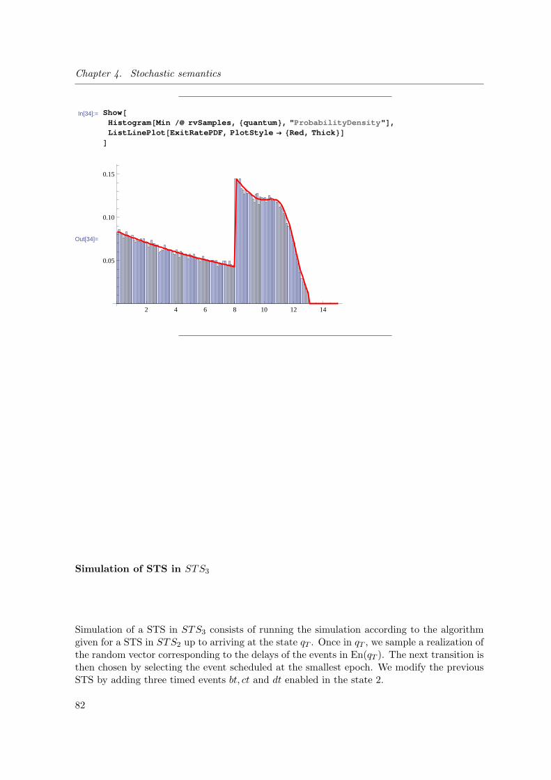
Chapter 4. Stochastic semantics
In[34]:= Show@Histogram @Min rvSamples, 8quantum <, " ProbabilityDensity " D,ListLinePlot @ExitRatePDF, PlotStyle ® 8Red, Thick <DD
Out[34]=
2 4 6 8 10 12 14
0.05
0.10
0.15
Simulation of STS in STS3
Simulation of a STS in STS3 consists of running the simulation according to the algorithmgiven for a STS in STS2 up to arriving at the state qT . Once in qT , we sample a realization ofthe random vector corresponding to the delays of the events in En(qT ). The next transition isthen chosen by selecting the event scheduled at the smallest epoch. We modify the previousSTS by adding three timed events bt, ct and dt enabled in the state 2.
82

4.3. Finite dimensional measures of the underlying stochastic process
In[37]:= S = 8a, b, c, d, dt , bt , ct <;W@Σ_D : = Switch @Σ , " init ", 1, a, 1, b, 2, c, 1, d, 5 DQ= 81, 2, 3, 4, 5, 6 <;G@Σ_D : = Switch @Σ , " init ", 0, a, 0, b, 0, c, 0, d, 0,
dt , NormalDistribution @12, 1 D,bt , ExponentialDistribution @1 12D,ct , UniformDistribution @88, 13 <DD
S = 881 ® 2, a<, 81 ® 3, b<, 81 ® 4, c<,82 ® 6, bt <, 82 ® 5, dt <, 82 ® 4, ct <,83 ® 4, b<,85 ® 6, a<, 85 ® 1, d<, 84 ® 1, b<,86 ® 6, a<<;
GraphPlot @S, DirectedEdges ® True, VertexLabeling ® True D
Out[42]= a
b
cbt
dt
ct
bb
a
a
d1
2
3
4
6
5
Simulation of such STS is carried out as follows. Once the set of enabled events in the currentstate is computed, we associate each event to a sample from the delays distribution. Fromthis sample list, we select the set of events that are associated with the smallest delay, then inthe case of ties (i.e. in STS3, for delays following a Dirac distribution), we apply the weightscheduler W1 to elect the winning event.
83

Chapter 4. Stochastic semantics
In[43]:= EnabledIn @s_D : = Select @S, ð@@1, 1 DD s &DPAll, 2 TTransitionFrom @s_, e_D : = Select @S, MatchQ @ð, 8s ® _, e<D &DP1T
In[45]:= Sample @f_D : =If @Head@fD === Integer, f,
RandomReal@fDD
In[46]:= Step @Ω_, W_D : = Module B8sfin , enabled , newWeights , totalWeight , nextE ,clocks , winners , nextT , winnerLabels , currentT <,
sfin = ΩP-1, 2 T;currentT = ΩP-1, 4 T;enabled = EnabledIn @sfin D;clocks = Hð1 -> Sample @G@ð1DDL & enabled ;clocks = GatherBy @clocks , ðP2T &D;winners = SortBy @clocks , ðP1, 2 T &DP1T;8nextT , winnerLabels < = 8winners P1, 2 T, winners PAll, 1 T<;nextE = If BLength @winnerLabels D == 1, winnerLabels P1T,
newWeights =W@Ω, ðD & winnerLabels ;totalWeight = Total @newWeights D;
RandomChoice B newWeights
totalWeight® winnerLabels F
F;
Return @Append@Ω, 8sfin , TransitionFrom @sfin , nextE DP1, 2 T, nextE ,currentT + nextT <DD
FW1@Ω_, Σ_D : = If @W@ΣD =!= Û, W@ΣD, 1 DStep1 @Ω_D : = Step @Ω, W1D
In[49]:= Nest @Step1, 881, 1, " init ", 0 <<, 20 DNest @Step1, 881, 1, " init ", 0 <<, 20 DNest @Step1, 881, 1, " init ", 0 <<, 20 D
Out[49]= 881, 1, init, 0<, 81, 3, b, 0<, 83, 4, b, 0<, 84, 1, b, 0<, 81, 4, c, 0<,84, 1, b, 0<, 81, 2, a, 0<, 82, 4, ct, 9.88599<, 84, 1, b, 9.88599<,81, 3, b, 9.88599<, 83, 4, b, 9.88599<, 84, 1, b, 9.88599<,81, 3, b, 9.88599<, 83, 4, b, 9.88599<, 84, 1, b, 9.88599<,81, 2, a, 9.88599<, 82, 6, bt, 11.7483<, 86, 6, a, 11.7483<,86, 6, a, 11.7483<, 86, 6, a, 11.7483<, 86, 6, a, 11.7483<<
Out[50]= 881, 1, init, 0<, 81, 4, c, 0<, 84, 1, b, 0<, 81, 3, b, 0<,83, 4, b, 0<, 84, 1, b, 0<, 81, 4, c, 0<, 84, 1, b, 0<,81, 3, b, 0<, 83, 4, b, 0<, 84, 1, b, 0<, 81, 4, c, 0<,84, 1, b, 0<, 81, 4, c, 0<, 84, 1, b, 0<, 81, 3, b, 0<,83, 4, b, 0<, 84, 1, b, 0<, 81, 4, c, 0<, 84, 1, b, 0<, 81, 2, a, 0<<
Out[51]= 881, 1, init, 0<, 81, 3, b, 0<, 83, 4, b, 0<, 84, 1, b, 0<, 81, 3, b, 0<,83, 4, b, 0<, 84, 1, b, 0<, 81, 2, a, 0<, 82, 6, bt, 5.3873<,86, 6, a, 5.3873<, 86, 6, a, 5.3873<, 86, 6, a, 5.3873<, 86, 6, a, 5.3873<,86, 6, a, 5.3873<, 86, 6, a, 5.3873<, 86, 6, a, 5.3873<, 86, 6, a, 5.3873<,86, 6, a, 5.3873<, 86, 6, a, 5.3873<, 86, 6, a, 5.3873<, 86, 6, a, 5.3873<<
84

4.3. Finite dimensional measures of the underlying stochastic process
Suppose that we want to compute P3(ω) for ω being one of(1
a,0−−→ 2dt,10−−−→ 5
a,0−−→ 6),
(1a,0−−→ 2
bt,6−−→ 6a,0−−→ 6), (1
a,0−−→ 2ct,20−−−→ 5
a,0−−→ 6), (1a,0−−→ 2
bt,14−−−→ 5a,0−−→ 6)
The empirical
estimators of the probabilities of these sojourn paths is computed as follows.
In[52]:= samples = Table @Nest @Step1, 881, 1, " init ", 0 <<, 3 D, 850 000 <D;
In[71]:= Untime @w_D : = w@@All, 1 ;; 3 DD
IsIn Ω@s_D : = Untime @sD 881, 1, " init " <, 81, 2, a<, 82, 5, dt <, 85, 6, a<< ì s@@3, 4 DD £ 10
IsIn Ω2@s_D : = Untime @sD 881, 1, " init " <, 81, 2, a<, 82, 6, bt <, 86, 6, a<< ì s@@3, 4 DD £ 6
IsIn Ω3@s_D : = Untime @sD 881, 1, " init " <, 81, 2, a<, 82, 4, ct <, 84, 1, b<< ì s@@3, 4 DD £ 20
IsIn Ω4@s_D : = Untime @sD 881, 1, " init " <, 81, 2, a<, 82, 6, bt <, 86, 6, a<< ì s@@3, 4 DD £ 14
In[76]:= emp =Length @Select @samples, ðDD
Length @samples D& 8IsIn Ω, IsIn Ω2, IsIn Ω3, IsIn Ω4<
N@%D
Out[76]= :7
25 000,
61
625,
2161
25 000,
359
2500>
Out[77]= 80.00028, 0.0976, 0.08644, 0.1436<
We compare the empirical estimators with the theoretical probability.
85

Chapter 4. Stochastic semantics
In[60]:= Prob2 @Ω_, W_D : = Module B8<,
MapIndexed B
Module B8Ωi , prefix , qi , Σi , conflicting , currentWeights , totalWeight <,Ωi = ΩPFirst @ð2DT;prefix = ΩP ;; First @ð2DT;Σi = Ωi P3T;qi = Ωi P1T;conflicting = EnabledIn @qi D;currentWeights =W@prefix , ðD & conflicting ;totalWeight = Total @currentWeights D;W@prefix , Σi D
totalWeight
F &, ΩF
F
In[61]:= ProbDWinsBeforeT @t_D : =NIntegrate @H1 - CDF@G@bt D, dDL*H1 - CDF@G@ct D, dDL*PDF@G@dt D, dD, 8d, 0, t<D
ProbBWinsBeforeT @t_D : =NIntegrate @H1 - CDF@G@dt D, bDL*H1 - CDF@G@ct D, bDL*PDF@G@bt D, bD, 8b, 0, t<D
ProbCWinsBeforeT @t_D : =NIntegrate @H1 - CDF@G@dt D, cDL*H1 - CDF@G@bt D, cDL*PDF@G@ct D, cD, 8c, 0, t<D
In[67]:= theo = 8Times Prob2 @881, 2, a<<, W1D * ProbDWinsBeforeT @10D *
Times Prob2 @885, 6, a<<, W1D,Times Prob2 @881, 2, a<<, W1D * ProbBWinsBeforeT @6D *
Times Prob2 @886, 6, a<<, W1D,Times Prob2 @881, 2, a<<, W1D * ProbCWinsBeforeT @20D *
Times Prob2 @884, 1, b<<, W1D,Times Prob2 @881, 2, a<<, W1D * ProbBWinsBeforeT @12D *
Times Prob2 @886, 6, a<<, W1D<
Out[67]= 80.000287621, 0.0983673, 0.0851965, 0.143219<
In[70]:= theo - emp
Out[70]= 97.62069´10-6, 0.000767335, -0.00124353, -0.000380768=
86

4.3. Finite dimensional measures of the underlying stochastic process
4.3.5 Probability of a sojourn path of STS4: Accounting for one step timedtransitions with general delays
We now remove the continuous restrictions on the r.v.. In this case, since the distributionsΓ(e) can be either continuous or discrete, the probability of two epochs being equal may benon null. More formally, we define the class STS4 as follows.
Definition 4.13 (A). STS S = 〈Q,−→, Σ, W, Γ〉 is in STS4 if there exists a unique, distin-guished state qT ∈ Q such that for every other state q′ 6= qT in Q, for every event e in En(q′),we have Γ(e) = δ0 and for every event e in En(q),Γ(e) is defined.
Following similar arguments as for the case of STS3, the probability measure P4 is fun-damentally defined by the outcome of a race condition between events competing in En(qT ).This implies that we have to compute P(〈E = e, T ≤ t〉) for e and t given. We will establishthat
P(〈E = e, T ≤ t〉) = (4.6)∑
E∈P(En(qT )−e)
(we,e′ ×
∫ t0
(∏e′∈En(qT )−E−e(1− Fe′(x))×∏e′∈E∪e fe′(x)
)dx)
.
where we,E is a weight value dependent on the conflict between e and the set E .
Proof. The proof is again carried out explicitly for three events En(qT ) = e1, e2, e3. Thebeginning of the proof follows the same principle as before, and thus we start with the equation(4.2), that is
P(E = e1, T ≤ t) = P(X ≤ t, X < Y, X < Z) (4.7)
+ a×P(X ≤ t, X = Y,X < Z)
+ b×P(X ≤ t, X = Z, X < Y )
+ c×P(X ≤ t, X = Z = Y ).
We will prove that each of the four terms of the sum in equation (4.7) corresponds to aterm of the sum of the equation (4.7). Let E be one of the subsets of P(En(qT ) − e1) =P(e2, e3) = ∅, e2 , e3 , e2, e3.
By equation (4.1), we can compute that the first term of (4.2) is
P(X ≤ t, X < Y, X < Z) =
∫ t
0(1− FY (x))× (1− FZ(x))× fX(x)dx. (4.8)
Consider the terms of the sum in equation (4.7). When E = ∅ we have En(qT )−E −e1 =e2, e3 and En(qT ) ∪ e1 = e1. Hence the term of the sum corresponding to E = ∅ yieldsequation (4.8).
Consider now the second term of equation (4.2). We have
P(X ≤ t, X = Y, X ≤ Z) =
∫ t
0(1− FZ(x))× fY (x)× fX(x)dx.
In the case of E = e2, we have En(qT ) − E − e1 = e3 and En(qT ) ∪ e1 = e1, e2.Therefore, the second term of the sum (4.7) yields equation (4.9).
87

Chapter 4. Stochastic semantics
Similarly,
P(X ≤ t, X = Y = Z) =
∫ t
0fZ(x)× fY (x)× fX(x)dt (4.9)
is the last term of the sum (4.7) and of the sum (4.7).
Property 4.6 (Exit rate). In the case where the r.v. denoting the delays of the events inEn(qT ) can be either continuous or discrete, we have the marginal distribution
P(T ≤ t) = 1−(∏
e∈Σs
(1− Fe(t))
). (4.10)
This marginal distribution does not depends on the weight function W and hence does notdepend on a weight scheduler W.
Proof. (Sketch) Since we built a mapping between each terms of equation (4.2) and (4.7), wewill work on (4.2). In the case of three variables X, Y, Z, notice that the terms P(X ≤ t, X =Z = Y ),P(Y ≤ t, X = Y = Z),P(Z ≤ t, X = Y = Z) of (4.2) are measures of the same set.These terms appears with different weights in the sum P(T ≤ t) =
∑e∈En(qT ) P(E = e, T ≤ t).
These weights sums to 1. Therefore we can factorize these three terms, and sum the weightsto 1. Hence, W does not appear in the marginal distribution.
Simarly as the case for P3, we decompose a sojourn path ω into probabilistically indepen-dent sub paths (ωi)i≤k and reuse P2 whenever possible.
Definition 4.14 (Measure P4). For a STS S = 〈Q,−→,Σ, W, Γ〉 in STS4, for a weightschedulerW, for any sojourn path ω of length greater or equal than 1 with the decomposition(ωi)i≤k then we define
P4(ω) = P2W(ω)×∏
0≤i≤k
P(〈E = ei, T ≤ ti〉)×
∑e∈En(qT )
∑n
q′|qT
e−→q′oW(ω | i, e, q′)
W(ω | i, ei, qT i)
where
P(〈E = ei, T ≤ ti〉) =
∑
E∈P(En(qT )−ei)
wei,E ×∫ ti
0
∏
e′∈En(qT )−E−ei
(1− Fe′(x))×∏
e′∈E∪ei
fe′(x)
dx
.
where
wei,E =W(ω | i, ei, qT i)∑
e′∈E∪e
∑
q′|qT
e′−→q′ffW(ω | i, e, q′) .
For the border cases where ω has a length 0, we set P4(ω) = 1.
88

4.3. Finite dimensional measures of the underlying stochastic process
Properties of STS in STS4
We can relate the measure P4 with the measure P2 and P3 as follows.
Property 4.7 (Relation with P2 and P3). For a STS S, for a weight scheduler W, if Sis in STS2, then for any sojourn path ω, we have P2,W(ω) = P4(ω). If S is in STS3, thenfor any sojourn path ω, we have P3(ω) = P4(ω).
Proof. Let S be a STS in STS2, by definition, Γ(e) = δ0 for e ∈ Σ. Let qT be any state ofS, we have S in STS4. Without loss of generality, assume that ω is a sojourn path where qT
is the one last state but one, and that it ends with (qT , (e1, t1), qT1. Thus, the decompositionof ω is ω itself. We have by definition Def. 4.14
P4(ω) = P2(ω)×P(E = e1, T ≤ t1)×
∑e∈En(qT )
∑n
q′|qT
e−→q′oW(ω, e, q′)
W(ω, e1, qT1)
with
P(〈E = e1, T ≤ ti〉) = (4.11)
∑
E∈P(En(qT )−e1)
we1,E ×∫ t1
0
∏
e′∈En(qT )−E−e1
(1− Fe′(x))×∏
e′∈E∪e1
fe′(x)
dx
.
with
we1,E =W(ω, e1, qT1)∑
e′∈E∪e1
∑
q′|qT
e′−→q′ffW(ω, e, q′)
.
Since Γ(e) = δ0 for each e ∈ Σ, P(X < Y ) = 0 and P(X = Y,X ≤ t) = 1 for X and Xbeing two r.v. distributed as δ0. Thus any term in the sum of the equation Eq. 4.12 whereE 6= En(qT )− e1 is null, and thus equation Eq. 4.12 reduces to we1,En(()qT )−ei
. We have
we1,En(qT )−ei=
W(ω, e1, qT1)∑e′∈En(qT )
∑
q′|qT
e′−→q′ffW(ω, e′, q′)
. (4.12)
Hence, we have
P4(ω) = P2W(ω)× W(ω, e1, qT1)∑e′ En(qT )
∑
q′|qT
e′−→q′ffW(ω, e, q′)
×
∑e∈En(qT )
∑n
q′|qT
e−→q′oW(ω, e, q′)
W(ω, e1, qT1)
= P2W(ω).
The case for P3(ω) = P4(ω) follows similar arguments: The probability P(X = Y ) for twor.v. with continuous distribution is equal to P(X = Y ) = 0, thus terms appearing in the sumP(〈E = e, T ≤ t〉) reduces to 0 except for the case when E = ∅, and thus we have
we1,∅ =W(ω, e1, qT1)∑
e′∈e1
∑
q′|qT
e′−→q′ffW(ω, e, q′)
=W(ω, e1, qT1)∑
q′|qT
e1−→q′ffW(ω, e1, q′)
,
89

Chapter 4. Stochastic semantics
and thus
P4(ω) = P2W(ω) ×∫ t1
0
∏
e′∈En(qT )−e1
(1− Fe′(t))
∗ fe1(t)dt
× (((((((W(ω, e1, qT1)∑
q′|qT
e1−→q′ffW(ω, e1, q′)
×
∑e∈En(qT )
∑n
q′|qT
e−→q′oW(ω, e, q′)
(((((((W(ω, e1, qT1)= P3(ω).
Property 4.8 (Instantaneous weighted transitions). Let S = 〈Q,−→,Σ, W, Γ〉 be aSTS, W be a weight scheduler for S, and ω be a sojourn path of S ending in a state q. If theset En(q) of events enabled in q contains an event e ∈ Σ such that Γ(e) = δ0, then for everye′ ∈ En(q) where P(X = 0) = 0 for a random variable X ∼ Γ(e′), we have P(E = e′) = 0.
Proof. Immediate by application of the marginal 4.4. For a random variable X ∼ δ0, we havefor any t ≥ 0, FX(t) = 1, and thus P(E = e) = 0 for any delay distribution Γ(e) such that0 /∈ supp(Γ(e)).
Numerical validation To validate numerically the definition 4.14, we merely have to val-idate the formula (4.7). To this end, we compute the probability that a random variableT that is distributed along a discrete uniform distribution over [5, 14] wins a race againstthree random variables X,Y, U such that X is normally distributed, Y is distributed alonga (continuous) uniform distribution over [8, 13] and U is distributed along a poisson distri-bution with rate 25. In order to resolve ties, we have W (T ) = 5 and W (U) = 7. Whencomparing the theoretical value with an empirical estimator over 30000, we obtain a totalerror of less than 0.03.
90

4.3. Finite dimensional measures of the underlying stochastic process
In[56]:= X = NormalDistribution @12, 1 D;Y = UniformDistribution @88, 13 <D;T = DiscreteUniformDistribution @85, 14 <D;U = PoissonDistribution @25D;
In[23]:= rvSamples = Table @Join @RandomReal 8X, Y<, RandomInteger 8T, U<D,830 000 <D;
In[60]:= wT = 5;wU= 7;
In[62]:= ElectWinner @s_D : = Module @8winnerIdx , winnerLbl <,winnerIdx = Ordering @sD@@1DD;winnerLbl = winnerIdx . 81 ® " X", 2 ® " Y", 3 ® " T", 4 ® " U" <;winnerLbl = If @winnerLbl " T" ì s@@3DD s@@4DD,
RandomChoice @8wT, wU< ® 8" T", " U" <D, winnerLbl D;8winnerLbl , s@@winnerIdx DD<D
In[63]:= winners = ElectWinner rvSamples;
In[64]:= XisSmallestAndLessThanT @t_D : =Select @winners, ð@@1DD " X" ì ð@@2DD £ t &D;
YisSmallestAndLessThanT @t_D : =Select @winners, ð@@1DD " Y" ì ð@@2DD £ t &D;
TisSmallestAndLessThanT @t_D : =Select @winners, ð@@1DD " T" ì ð@@2DD £ t &D;
UisSmallestAndLessThanT @t_D : = Select @winners, ð@@1DD " U" ì ð@@2DD £ t &D;
In[68]:= TWins@t_D : = NBSum@H1 - CDF@X, tv DL*H1 - CDF@Y, tv DL*H1 - CDF@U, tv DL*PDF@T, tv D,8tv , 0, t<D+ Sum@H1 - CDF@X, tv DL*H1 - CDF@Y, tv DL*PDF@U, tv D*PDF@T, tv D,8tv , 0, t<D* wT
wU+ wT
F
In[71]:= Total BTable BNormBTWins@t D - Length @TisSmallestAndLessThanT @t DDLength @rvSamples D
F,
8t , 2, 14, 0.5 <FF
Out[71]= 0.0232144
Similarly to the numerical validation performed for STS3, we compute the theoreticalmarginal distribution as follows.
91

Chapter 4. Stochastic semantics
In[50]:= ExitRate @t_D : =1 - H1 - CDF@X, tDL*H1 - CDF@Y, tDL*H1 - CDF@T, tDL*H1 - CDF@U, tDL
In[51]:= ExitRateCDF = Table @8t , ExitRate @t D<, 8t , 0, 15, quantum <D;ListLinePlot @ExitRateCDF, PlotStyle ® 8Red, Thick <D
Out[52]=
2 4 6 8 10 12 14
0.2
0.4
0.6
0.8
1.0
In[53]:= ExitRatePDF = Transpose @8ExitRateCDF @@2 ;;, 1 DD,Differences @ExitRateCDF @@All, 2 DDD*1 quantum <
D;ListLinePlot @ExitRatePDF, PlotStyle ® 8Red, Thick <, PlotRange ® All D
Out[54]=
2 4 6 8 10 12 14
0.2
0.4
0.6
0.8
1.0
And we can compare the theoretical marginal distributions with the empirical one by plot-ting both on the same plot.
92
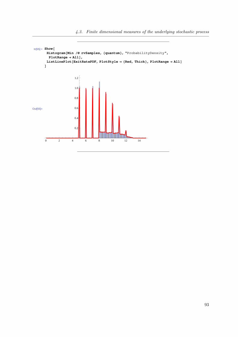
4.3. Finite dimensional measures of the underlying stochastic process
In[55]:= Show@Histogram @Min rvSamples, 8quantum <, " ProbabilityDensity ",
PlotRange ® All D,ListLinePlot @ExitRatePDF, PlotStyle ® 8Red, Thick <, PlotRange ® All DD
Out[55]=
0 2 4 6 8 10 12 14
0.2
0.4
0.6
0.8
1.0
1.2
93

Chapter 4. Stochastic semantics
4.3.6 Probability of a sojourn path in STS5: Accounting for elapsed timesince regeneration
We suppose that we want to compute the probability of a sojourn path (Q, a, t0, R, b, t1, S).In the initial state of this path, the process is at the global epoch 0, the process hits Q a firsttime and the timers of events enabled in Q are sampled accordingly to the probability lawsdefined by Γ. Suppose that we have En(()Q) = a, b, c. At the epoch where the process hitsthe state Q, we say that the state Q regenerates the events a, b, c (or equivalently that Qis regenerative for the events a, b, c). Let A, B,C be three r.v. representing the timers of theevents a, b, c at the epoch 0.
The probability of the prefix sojourn path (Q, a, t0, R) is given by P4. Once in R, the
probability of taking the transition Rb−→ S while sojourning in R less than t1 time units
depends on the outcome of the race condition between the events b, c. However, contraryto the race condition in Q, we do not resample the timers of these events and thus the racecondition in R must account for time that was elapsed since the epoch where the timers of band c were sampled. This implies that the outcome of the race condition in R is dependenton the outcome of the race condition in Q, and more precisely of the sojourn time in Q.
Suppose that in Q, the sampled clocks were 〈A : a, B : b, C : c〉. The sojourn time in thestate Q is thus a t.u., and the epoch of arrival in state R is also a. In order for the eventb to wins the second race with a sojourn time in the state R less than t1, we must haveb < t1 + a ∧ b < c. This implies that the probability of the sojourn path (Q, a, t0, R, b, t1, S)is given by
P(A < t0, A < B, A < C,B < t1 + A, B < C) = P(A < t0, A < B < t1 + A, B < C),
and since all these (probabilistic) events are dependent, this probability cannot be decom-posed in a product of probabilities. However the subset of R3 satisfying the inequalitiesa < t0 ∧ a < b < t1 + a ∧ b < c is a c, b, a-simple domain, and we can thus evaluate this prob-ability by repeated integration as follows
P (A < t0, A < B < t1 + A, B < C) =
∫
a<t0,a<b<t1+a,b<cfA(a) · fB(b) · fC(c)
=
∫ t0
0fA(a)
∫ t1+a
afB(b)
∫ +∞
bfC(c)dcdbda
=
∫ t0
0fA(a)
∫ t1+a
afB(b) ∗ (1− FC(b)) dbda.
We now generalize the previous construction and formally define the class STS5 that areSTS5 where all the timers of the timed events are always regenerated at the same epoch. Wewill then express a sojourn path as a conjunction of constraints over n r.v. variables, where n isthe number of events. We will then show that the region of R
n satisfying this conjunction is asimple domain of R
n and thus that we can use repeated integration to measure its probability.In order to compute the probability that the sojourn time in a state q is less that an
threshold value t when taking a transition labeled by the event e, we must account for thetime elapsed since the regeneration of the clock of the event e. This regeneration happenswhen the event e became enabled for the first time when reaching a state. More formally, wehave :
94

4.3. Finite dimensional measures of the underlying stochastic process
Definition 4.15 (Events regenerated by a transition). Let qe−→ q′ be a transition of a
STS S = 〈Q,−→,Σ, W, Γ〉. The events regenerated by this transition are
Reg(qe−→ q′) = (En(q′)− En(q)) ∪ (En(q′) ∩ e)
And thus, we can define the class STS5 as follows.
Definition 4.16 (STS5). Let S = 〈Q,−→,Σ, W, Γ〉 be a STS. It is in STS5 if for anytransition q
e−→ q′ we have either Reg(qe−→ q′) = ΣT or we have Reg(q
e−→ q′) ∪ ΣT = ∅, whereΣT = e ∈ Σ | Γ(e) 6= δ0 is the set of timed events in S.
Regenerative steps corresponds to a probabilistic reset in the underlying stochastic process.In other words, once a regenerative step is taken, the future state of the stochastic processdoes not depends on what happened before the regenerative step. In order to define the finiteprobability of a sojourn path, we will first assume that the sojourn path starts with a statewhere timed events are enabled, then remove this restriction and show that we can decomposea sojourn path into probabilistically independent sub-paths where each sub-path starts witha state where timed events are enabled.
Definition 4.17 (Non regenerative sojourn paths). Let ω = (q0, (ei, ti, qi)i≤n) be asojourn path of a STS S = 〈Q,−→,Σ, W, Γ〉 in STS5. We say that ω is not regenerative if
we have En(q0) ∩ ΣT 6= ∅ and if Reg(qiei−→ qi+1 = ∅ for all i ≥ 0.
We first characterize the probability of non regenerative paths. To this end, we first have :
Lemma 4.9. If ω is not regenerative, then
• no event in ω appears more than once,
• ei ⊆ En(q0),
• En(qi+1) ⊂ En(qi).
Since no event appears more than once in ω and since all the clocks of the (timed) eventsin ω are sampled at the same state and at the same epoch, we can consider a single r.v. C(e)denoting the value of the clock of the event e. We can already model the fact that the evente has an activity delay following Γ(e) by setting C(e) ∼ Γ(e).
Let qi be a state appearing in ω and let the r.v. Epoch(qi) denotes the epoch when theprocess reach the state qi. The state qi is reached after firing the event ei−1 during the
transition qi−1ei−1−−−→ qi. Since the clock C(ei−1) is sampled only once at epoch 0, we have
Epoch(qi) = C(ei−1).In any state qi of ω, the sojourn time Ti must be less that ti. This sojourn time in the
state qi is the r.v. Epoch(qi+1)−Epoch(qi). Since Epoch(qi) = C(ei−1), the sojourn time Ti
is Ti = C(ei)− C(ei−1) for i > 1. For the first sojourn time T0, we have T0 = C(e0).Finally, in order for an event ei to win the race condition between the competing events in
En(qi), we must have∧
e∈En(qi)
C(ei) ≤ C(e).
Thus we have P(ω) =
P(Q0 = q0, E0 = e0, T0 ≤ t0, Q1 = q1, E1 = e1, T1 ≤ t1, . . . , Qn = qn, En = en, Tn ≤ tn) =
95

Chapter 4. Stochastic semantics
P(C(e0) ≤ t0 ∧∧
e∈En(q0)
C(e0) < C(e) ∧∧
i≤n
C(ei)− C(ei−1) ≤ ti ∧∧
e∈En(qi)
C(ei) ≤ C(e)).
In order to compute this probability via integration, we express it as a n + 1-dimensionalregion of R
n+1+ with axes labeled in order by c0, . . . , cn. Since every events in ω appears only
once, let ind(e) be the index value i such that ind(e) = i if e = ei. Let R be the region defined
by the inequalities R =
c0 ≤ t0 ∧
∧
e∈En(q0)
c0 ≤ cind(e) ∧∧
i≤nci − ci−1 ∧
∧
e∈En(qi)
ci ≤ cind(e)
.
Since all the clocks r.v. Ci are independent, we have
P(ω) =
∫
〈c0,c1,...,cn〉∈R
∏
0≤i≤n
fi(ci), (4.13)
where fi is the probability density function of Γ(ei).
Property 4.10 (Simplicity of R). The region R is equal to the (cn, . . . , c0)-simple domainD represented by the inequalities
D = c0 ≤ t0 ∧ c0 ≤ c1 ≤ c0 + t1 ∧ · · · ∧ cn−1 ≤ cn ≤ cn−1 + tn .
Proof. Since∧
i≤nci − ci−1 ≤ ti is one of the terms in the inequalities of R, we have R ⊆ D.
Let 〈c0, . . . , cn〉 be an element of D. By transitivity, we know that for every index i, we haveci ≤ cj if j > i. Since we have En(qi+1) ⊂ En(qi), we have ind(e) > i for e ∈ En(qi). Thus,we have ci < cind(e) for all e ∈ En(qi).
We now restrict the following formulas to the case where all r.v. are absolutely continuous.Since R and D are the same subset of R
n+1+ , since D is (cn, . . . , c0)-simple, we can repeatedly
integrate the right hand side of 4.13 and thus we have P(ω) =
∫ t0
0
(f0(x0) ·
∫ x0+t1
x0
(f1(x1) ·
∫ x1+t2
x1
(f2(x2) · · ·
∫ xn−1+tn
xn−1
fn(xn)dxndxn−1 . . .
)dx2
)dx1
)dx0.
(4.14)We now remove the restriction on ω and consider paths with multiple regeneration points.
Let ω be a sojourn path in a STS S = 〈Q,−→,Σ, W, Γ〉. The decomposition of ω intoprobabilistically independent sub paths ω = ω1ω2ω3 . . . ωn is the sequence of sub paths (ωi)i≤n
where ωi ends with a transition qe−→ q′ such that Reg(q
e−→ q′) = ΣT . Since all clocks areregenerated at the end of a sub-path ωi, two consecutive sub paths are probabilisticallyindependent and any sub-path ωi is not regenerative.
96

4.3. Finite dimensional measures of the underlying stochastic process
Simulation of STS in STS5
We consider a STS with non regenerative paths of length 2.
S = 8a, b, c, d, dt , bt , ct <;W@Σ_D : = Switch @Σ , " init ", 1, a, 10, b, 2, c, 1, d, 5 DQ= 81, 2, 3, 4, 5, 6 <;G@Σ_D : = Switch @Σ , " init ", 0, a, 0, b, 0, c, 0, d, 0,
bt , NormalDistribution @12, 3 D,ct , UniformDistribution @89, 12 <D,dt , NormalDistribution @8, 1 DD
S = 881 ® 2, a<, 81 ® 3, b<, 81 ® 4, c<,82 ® 6, bt <, 82 ® 5, dt <, 82 ® 4, ct <,83 ® 4, b<,85 ® 6, bt <, 85 ® 1, ct <, 84 ® 1, b<,86 ® 6, a<<;
GraphPlot @S, DirectedEdges ® True, VertexLabeling ® True D
a
b
cbt
dt
ct
bb
a
bt
ct1
2
3
4
6
5
In order to simulate this STS, we implement the variable time advance algorithm [She93] thatwas described in section sec. 4.3.1. To this end, we first define a function Regenerate(q,e,q’)
that returns the set of event that should be regenerated after the transition qe−→ q′. Note
that for STS in STS5, this function always return one of the sets: all the timed events, a setof untimed events, the empty set.
97

Chapter 4. Stochastic semantics
In[52]:= SetDiff @X_, Y_D : = Complement @X, Intersection @X, YDD
In[62]:= Regenerate @q_, e_, qp_D : =Union @SetDiff @EnabledIn @qpD, EnabledIn @qDD,
Intersection @EnabledIn @qpD, 8e<DD
Step @8Ω_, clocks_<, W_D : = Module B8sfin , enabled , newWeights , totalWeight , nextE ,minclocks , winners , nextT , nextS , winnerLabels , currentT ,nextClock , toRemove <,
sfin = ΩP-1, 2 T;currentT = ΩP-1, 4 T;If @Length @clocksD 0, Return @8Ω, 8<<DD;minclocks = GatherBy @clocks, ðP2T &D;winners = SortBy @minclocks , ðP1, 2 T &DP1T;8nextT , winnerLabels < = 8winners P1, 2 T, winners PAll, 1 T<;nextE = If BLength @winnerLabels D == 1, winnerLabels P1T,
newWeights =W@Ω, ðD & winnerLabels ;totalWeight = Total @newWeights D;
RandomChoice B newWeights
totalWeight® winnerLabels F
F;nextS = TransitionFrom @sfin , nextE DP1, 2 T;toRemove = SetDiff @EnabledIn @sfin D, EnabledIn @nextS DD;nextClock = Union @
Select @clocks, ð@@1DD =!= nextE ì Not @MemberQ@toRemove , ð@@1DDDD &D,Hð1 ® nextT + Sample @G@ð1DDL & Regenerate @sfin , nextE , nextS DD;
Return @8Append@Ω, 8sfin , nextS , nextE , nextT <D, nextClock <DF
W1@Ω_, Σ_D : = If @W@ΣD =!= Û, W@ΣD, 1 DStep1 @8Ω_, clock_<D : = Step @8Ω, clock<, W1D
In[66]:= Ω = 881, 1, " init ", 0 <<nextClock = Hð1 ® Sample @G@ð1DDL & EnabledIn @Ω@@-1, 2 DDDStep1 @8Ω, nextClock <D
Out[66]= 881, 1, init, 0<<
Out[67]= 8a ® 0, b ® 0, c ® 0<
Out[68]= 8881, 1, init, 0<, 81, 2, a, 0<<, 8bt ® 15.7947, ct ® 9.44422, dt ® 7.44469<<
We now compare the exact probability (as given by Eq. (4.14)) with an empirical estimation.The empirical estimation of the path
1a,0−−→ 2
dt,d1−−−→ 5ct,d2−−−→ 1
a,0−−→ 2dt,d1−−−→ 5
ct,d2−−−→ 1a,0−−→ 2
dt,d1−−−→ 5
is given by the following code.
98

4.3. Finite dimensional measures of the underlying stochastic process
In[96]:= IsInL1TimedWithDeadlines @s_, d1_, d2_D : =Untime @sD exPath && VectorLessEqual @Time @sD, 80, d1, d2, 0, d1, d2, 0, d1<D
In[97]:= NBLength @Select @samples, IsInL1TimedWithDeadlines @ð, 8, 4 D &DDLength @samples D
F
Out[97]= 0.01645
while the theoretical value is given by
In[92]:= d1 = 8;d2 = 4;
In[94]:= 10 13 *NIntegrate @H1 - CDF@G@bt D, cDL*PDF@G@ct D, cD*PDF@G@dt D, dD,8d, 0, d1 <, 8c, d, d + d2<D*
10 13 *NIntegrate @H1 - CDF@G@bt D, cDL*PDF@G@ct D, cD*PDF@G@dt D, dD,8d, 0, d1 <, 8c, d, d + d2<D*
NIntegrate @H1 - CDF@G@bt D, dDL*H1 - CDF@G@ct D, dDL*PDF@G@dt D, dD,8d, 0, d1 <D
Out[94]= 0.0195693
99

Chapter 4. Stochastic semantics
4.3.7 Probability of a sojourn path in STS6: General case
In the general case, we must account for regeneration of clocks that do not happen at the sameepoch. This implies that in a given state, the clocks of competing events account for elapsedtime since regeneration (like in STS5) but also for a delay between regeneration epochs. Weillustrate this on the following example.
Example 4.1.
In[25]:= S = 88X ® Y, a<, 8X ® Æ, b<, 8X ® Æ, c<,8Y ® Z, b<, 8Y ® Æ, c<, 8Y ® Æ, d<, 8Y ® Æ, a<,8Z ® U, c<, 8Z ® Æ, a<, 8Z ® Æ, e<,8U® fWin , f <, 8U® eWin , e<, 8U® aWin , a<<;
G@Σ_D : = Switch @Σ ,a, NormalDistribution @15, 3 D,b, NormalDistribution @24, 3 D,c, UniformDistribution @815, 18 <D,d, NormalDistribution @8, 1 D,e, NormalDistribution @10, 2 D,f , ExponentialDistribution @1 3DD
TreePlot @S, Left, X, DirectedEdges ® True, VertexLabeling ® True D
a
bc
b
c da
c
ae
f
e
a
X Y
Æ
Z U
fWin
eWin
aWin
We will follow the clocks and regenerations as we step trough the path Xa−→ Y
b−→ Zc−→ U
e−→eWin in this STS. As we did for STS5, we will express this sojourn path as a conjunction ofconstraints over n clock variables, show that this conjunction yields a simple domain of R
n
and use repeated integration to measure the probability of this domain.Starting from state X, the initial clock structure is 〈A : a, B : b, C : c〉. Suppose that a
is the minimal epoch, the first step in S is thus Xa−→ Y . Once in Y , the global epoch is
set to a, the clocks of the events a, d are regenerated and thus the new clock structure is〈A : a + a′, B : b, C : c, D : d + a〉. Suppose now that the minimal epoch in the clock structure
is b. After the transition Yb−→ Z, the global epoch is set to b, and since the set of newly enabled
events is e, we update the clock structure and obtain 〈A : a + a′, C : c, E : e + b〉. If c is the
100

4.3. Finite dimensional measures of the underlying stochastic process
minimal epoch, after the transition Zc−→ U , the global epoch is set to c, and the clock structure
is updated to 〈A : a + a′, E : e + b, F : f + c〉. For this example, the race condition in the stateU involves three events whose delays are r.v. following a sum of independent and non identicalr.v.. Furthermore, in the state U , we must account for the elapsed time since regenerationand (equivalently) the races already lost, i.e. we have a + a′ > b ∧ a + a′ > c ∧ e + b > c.
In order to compute the probability of the sojourn path
ω = Xa,tX−−−→ Y
b,tY−−→ Zc,tZ−−→ U
e,tU−−→ eWin
where tX, tY, tZ, tU are real valued constants, we have to determine the regeneration epochof each event racing in each state of ω as well as all the races that has been lost. Considerfor example the sojourn time T4 in the last state. The sojourn path specify that T4 ≤ tU .The sojourn r.v. T4 is equal to Epoch(eWin)−Epoch(U). The r.v. Epoch(eWin) is definedas the sum Ce + Epoch(last regeneration of e) where Ce ∼ Γ(e). Since the event e has been
regenerated after the transition Yb−→ Z, we have Epoch(last regeneration of e) = Epoch(Z).
The r.v. Epoch(Z) is defined as Epoch(Z) = Cb −Epoch(last regeneration of b). Since b hasbeen regenerated when reaching the initial state X, we have Epoch(last regeneration of b) =Epoch(X) = 0, and thus Epoch(Z) = Cb and thus Epoch(eWin) = Ce + Cb. Similarly, wehave
Epoch(U) = Cc + Epoch(last regeneration of c) = Cc + Epoch(X) = Cc
and thus we have T4 ≤ tU = Ce + Cb − Cc < tU. Furthermore, in the state U , ther.v. representing the epoch of firing the event e is Ce + Cb. For the event a, it is Ca +Epoch(last regeneration of a), with Epoch(last regeneration of a) = Epoch(Y ) = C ′
a andthus the epoch of firing the event a is Ca + C ′
a. Finally, for the event f , the epoch offiring is Cf + Epoch(U) = Cf + Cc. This implies that in the state U , the sojourn time is lessthan tU and the event e wins if
Cb + Ce < Ca + C ′a ∧ Cb + Ce < Cc + Cf ∧ Cb + Ce − Cc < tU.
which can be restated as the following a, b, c, e, d, f, a′-simple domain
Ce < tU − Cb + Cc ∧ Cf > Cb − Cc + Ce ∧ a′ > −Ca + Cb + Ce
where each Cl is a r.v. following Γ(l).By performing similar computation, the event c wins in state Z in less than tZ t.u. if
Cc < Cb + tZ ∧ Ce > Cc − Cb ∧ C ′a > Cc − Ca.
In state Y , the event b wins in less than tY t.u. if
Cb < Ca + tZ ∧ Cc > Cb ∧ Cd > Cb − Ca ∧ C ′a > Cb − Ca.
In state X, the event a wins in less than tX t.u. if
Ca < tX ∧ Cb > Ca ∧ Cc > Ca.
Finally, the probability P(ω) of the sojourn path ω is
P( 0 < Ca < tX ∧ Ca < Ca < Ca + tY ∧ Ca < Cc < Ca + tZ ∧ Cc − Ca < Ce < −Ca + Cc + tU
∧Cd > Ca − Ca ∧ Cf > Ca − Cc + Ce ∧ C ′a > −Ca + Ca + Ce).
101

Chapter 4. Stochastic semantics
We now generalize this construction. Given a sojourn path ω, we want to express theconstraints over Q, E, T present in ω by constraints over Ce and t which are resp. r.v.denoting the value of the remaining activity delay of some event e and real valued constants.
Since STS6 are the general case, an event may be regenerated or appear multiple timesin ω. Let Σω be the multiset over Σ defined by Σω = Reg(qi
ei−→ qi+1)i≤n. An event e hasmultiplicity k if its timer is regenerated k times during a realization going trough the statesof ω. All these regenerated timers are different independent and identically distributed r.v.Ci(e) following Γ(e). Thus, even if n events appears in ω, its probability will involve card(Σω)different random variables. In order to avoid explicitly stating which r.v. represent the timerof the ith regeneration of e, we impose without loss of generality that all the multiplicities inΣω are 1. If it is not the case and since all the regeneration of a timer are independent andidentically distributed, we can augment Σ with unique labels e1, e2, . . . and update Γ and Waccordingly by setting Γ(ei) = Γ(e), W (ei) = W (e). We will then denote by C(e) the timerrandom variable associated with the event e and by χ the set of the timer r.v. of all theevents in Σω. Note that with the assumption that Σω has a multiplicity of 1 for each event,we have card(χ) = card(ω).
Given a sojourn path ω and an event e, the last regenerative state Regω(e) is the last stateof ω where the event e is regenerated. That is, Regω(e) maps an event e ∈ Σω to a stateq ∈ ω and is defined by
Regω(e) = qi, s.t e ∈ Reg(qiei−→ qi+1), and s.t. ∀j > i, e /∈ Reg(qj
ej−→ qj+1),
where Reg(qe−→ q′) is the function defined in Def. 4.15.
The r.v. Epochω(qi) representing the epoch at which the state qi is reached in the path ωis a linear combination of timer random variables. The function Epochω(qi) thus map a stateqi ∈ ω to a term over χ, and is defined recursively by
Epochω(qi) =
0 if |ω| = 0
C(e) + Epochω|i(Regω|i−1(e)) otherwise
where e is the event in Σω for which we have qi−1e−→ qi in ω. In the definition of Epochω(qi),
the term Epochω|i(Regω|i−1(e)) is a linear combination of timer r.v. representing the epochof regeneration of the event e.
By using Epochω(qi+1) we can describe the sojourn time in the state qi as being the dif-ference between the two successive epoch. More formally, the r.v. Sojournω(qi) representingthe sojourn time in state qi is a linear combination of timer r.v. and is defined by
Sojournω(qi) = Epochω(qi+1)− Epochω(qi).
Finally, the epoch at which a given event e fires can also be expressed in terms of timerrandom variables. For any event e in ω, we define the r.v. FiringEpochω(e) as
FiringEpochω(e) = C(e) + Epochω|−1(Regω(e)).
Both functions Sojourn and Epoch maps a state visited in ω to a linear combination oftimer random variables, while the function FiringEpoch maps an event fired in ω to a linearcombination of timer random variables. We now use these three functions to express the prob-abilistic event e wins the race in state qn before time tn as constraints over the realizationsof the timer random variables.
102

4.3. Finite dimensional measures of the underlying stochastic process
In the last state qn of ω, the sojourn time of the process is bounded by tn. Therefore, wealready must impose that
Sojournω(qn) ≤ tn.
Futhermore, for the event en to win the race condition in state qn, we must have∧
e′∈En(qn),e′ 6=en
FiringEpochω(en) ≤ FiringEpochω(e).
Then, for any sojourn path ω, we must have
∧
ei∈ω
(Sojournω|i(qi) ≤ ti ∧
∧
e∈En(qi),e′ 6=ei
(FiringEpochω|i(ei) ≤ FiringEpochω|i(e)
)).
(4.15)However the region of R
card(χ) satisfying this inequality is not simple and thus not amenableto measure with integration. Still, we can remark that Σω can be partitioned in the threepartitions:
• Winners(ω) = e | e ∈ ω,
• Delayed(ω) = e | e /∈ ω, e ∈ En(qn),
• Loosers(ω) = e | e /∈ ω, e /∈ En(qn),where Winners represent the set of events that won a race condition, Delayed the set ofevents that did not win any race condition but are still enabled and may thus win a futurerace condition, and where Loosers is the set of event that lost all race conditions and weredeactivated in some state visited by ω. For any event ei ∈ Winners, we know that in stateqi the event must fire before the deadline ti, ti being relative to the time at which the process
reached qi. Consider again the STS of the example Ex. 4.1, the sojourn path ω = Xa,tX−−−→
Yb,tY−−→ Z
c,tZ−−→ Ue,tU−−→ eWin, and particularly the three transitions Y
b−→ Zc−→ U
e−→ eWin.In the following, we omit the subscript ω. The sojourn in Z is given by
Sojourn(Z) = Epoch(U)− Epoch(Z)
C(c) + Epoch(Reg(c))− C(b)− Epoch(Reg(b)),
and the term
C(c)− Sojourn(Z) = C(c)−(C(c) + Epoch(Reg(c))− C(b)− Epoch(Reg(b))
)
C(c)− C(c)− Epoch(Reg(c)) + C(b) + Epoch(Reg(b))
C(b) + Epoch(Reg(b))− Epoch(Reg(C))
represent the firing epoch of b relatively to the regeneration of c. Since the system reachedthe state Z exactly at the firing epoch of b, we must have
C(b) + Epoch(Reg(b))− Epoch(Reg(C)) ≤ C(c) ≤ C(b) + Epoch(Reg(b))− Epoch(Reg(C)) + tZ
⇔ C(c)− Sojourn(Z) ≤ C(c) ≤ C(c)− Sojourn(Z) + tZ .
More generally, for any event ei such that qiei,ti−−→ qi+1 ∈ ω, we have
C(ei)− Sojourn(qi) ≤ C(ei) ≤ C(ei)− Sojourn(qi) + ti,
103

Chapter 4. Stochastic semantics
where the term C(ei) − Sojourn(qi) does not involve C(ei) and is a linear combination oftimer r.v. of the events that won the i first race.
For a delayed event e ∈ Delayed, we know that it lost all n race conditions, and thus thatfor every event ei ∈ ω, we have FiringEpochω|i(e) ≥ FiringEpochω|i(ei). However, for any i,we have FiringEpochω|i(ei) ≤ FiringEpochω|i+1(ei+1), and thus it is sufficient to impose forany delayed event e ∈ Delayed that
FiringEpochω(e) ≥ FiringEpochω(en).
Finally, for any event e ∈ Loosers, let Last(e) = qi be the state such that qiei−→ qi+1 and
e ∈ En(qi) and e /∈ En(qi+1). In words, Last(e) is the last state where e was active, and isthe state where it lost its last race. We must have
FiringEpochω|i(e) ≥ FiringEpochω|i(ei).
Now let Dω be the set of inequality over timer r.v. defined by
Dω =∧
ei∈Winners(ω)
(C(ei)− Sojourn(qi) ≤ C(ei) ≤ C(ei)− Sojourn(qi) + ti
)∧
∧
e∈Delayed(ω)
(FiringEpochω(e) ≥ FiringEpochω(en)
)∧
∧
e∈Loosers(ω),qi=Last(e)
(FiringEpochω|i(e) ≥ FiringEpochω|i(ei)
). (4.16)
Recall that we are given a rewriting such that all events appears with multiplicity one inΣω. Then the sequence ≺= ce0 , ce1 , . . . , cen , (ce)e∈Σω ,e/∈ω where we enumerate first the eventsappearing in ω in order, then all the events regenerated in ω in any fixed order is a completeorder over Σω. Label the axes of R
card(Σω) by ≺, then for a sojourn path ω, we have thefollowing property.
Property 4.11 (Simplicity of Dω). The region Dω ⊆ Rcard(χ) is a ≻-simple domain.
Proof. Consider in order the axes of ≺ and recall that each axis is associated to an uniqueevent e, and thus to a unique timer r.v. C(e). Let e be an event.
If e ∈ Winners(ω), then there exists i s.t. e = ei. Let j be the index of i in ≺, then therange in Dω of the variable cj associated with the r.v. C(ei) is constrained by
C(ei)− Sojourn(qi) ≤ C(ei) ≤ C(ei)− Sojourn(qi) + ti.
Since Sojourn(qi) is a linear combination over some timer r.v. in C(ek) such that k ≤ iand where C(ei) appears only once, the term C(ei)− Sojourn(qi) is a linear combination oftimer r.v. in C(ek), and thus the variable cj is bounded by variables of lower index.
If e ∈ Delayed, for the index j of e in ≺, the variable cj is constrained by
FiringEpochω(e) ≥ FiringEpochω(en)
and since by construction j is greater than the index of the axis associated with en, then thevariable cj is only dependent by variables of lower index.
Finally, if e ∈ Loosers, for the index j of e in ≺, the variable cj is constrained by
FiringEpochω|i(e) ≥ FiringEpochω|i(ei)
104
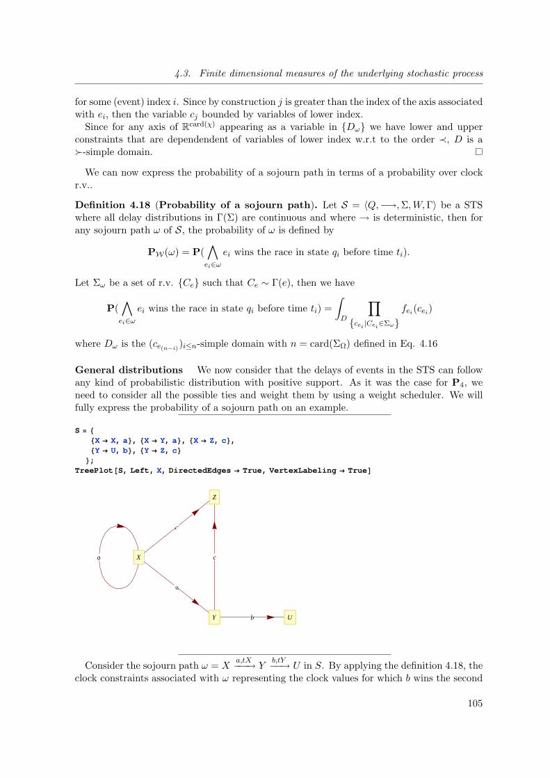
4.3. Finite dimensional measures of the underlying stochastic process
for some (event) index i. Since by construction j is greater than the index of the axis associatedwith ei, then the variable cj bounded by variables of lower index.
Since for any axis of Rcard(χ) appearing as a variable in Dω we have lower and upper
constraints that are dependendent of variables of lower index w.r.t to the order ≺, D is a≻-simple domain.
We can now express the probability of a sojourn path in terms of a probability over clockr.v..
Definition 4.18 (Probability of a sojourn path). Let S = 〈Q,−→, Σ, W, Γ〉 be a STSwhere all delay distributions in Γ(Σ) are continuous and where → is deterministic, then forany sojourn path ω of S, the probability of ω is defined by
PW(ω) = P(∧
ei∈ω
ei wins the race in state qi before time ti).
Let Σω be a set of r.v. Ce such that Ce ∼ Γ(e), then we have
P(∧
ei∈ω
ei wins the race in state qi before time ti) =
∫
D
∏
cei|Cei
∈Σωfei
(cei)
where Dω is the (ce(n−i))i≤n-simple domain with n = card(ΣΩ) defined in Eq. 4.16
General distributions We now consider that the delays of events in the STS can followany kind of probabilistic distribution with positive support. As it was the case for P4, weneed to consider all the possible ties and weight them by using a weight scheduler. We willfully express the probability of a sojourn path on an example.
S = 88X ® X, a<, 8X ® Y, a<, 8X ® Z, c<,8Y ® U, b<, 8Y ® Z, c<<;
TreePlot @S, Left, X, DirectedEdges ® True, VertexLabeling ® True D
a
a
c
b
cX
Y
Z
U
Consider the sojourn path ω = Xa,tX−−−→ Y
b,tY−−→ U in S. By applying the definition 4.18, theclock constraints associated with ω representing the clock values for which b wins the second
105

Chapter 4. Stochastic semantics
race condition before tU is Dω = 0 ≤ a < 8 ∧ 0 ≤ b < 12 ∧ c ≥ a + b. In the case wherethe clock r.v. can be either discrete or continuous, we have to account for all the possibleties. To this end, we decompose Dω into disjoint subsets by considering that any inequalityof the form a ≤ b is equivalent to the disjunction (a < b) ∨ (a = b). Therefore we have thedecomposition of Dω into 23 disjunct domains,
Dω = a = 0 ∧ b = 0 ∧ c = a + b∪ a = 0 ∧ b = 0 ∧ c > a + b∪ a = 0 ∧ 0 < b < 12 ∧ c > a + b∪ a = 0 ∧ 0 < b < 12 ∧ c = a + b∪ 0 < a < 8 ∧ b = 0 ∧ c = a + b∪ 0 < a < 8 ∧ b = 0 ∧ c > a + b∪ 0 < a < 8 ∧ 0 < b < 12 ∧ c = a + b∪ 0 < a < 8 ∧ 0 < b < 12 ∧ c > a + b.
Each of these sub-domains are simple domain and can be measured with formulas similar tothe one in definition Def. 4.18.
To each of this sub-domain, we associate a tie sequence. A tie sequence Σqq∈ω is asequence of subset of Σ indexed by the successive states in the sojourn path. Two events arein the same subset if their associated firing epoch are equals. In other words, each element ofa tie sequence Σq associated to a simple domain Di is a subset of the events En(q) in q forwhich the clock constraints in Di are not sufficient to determine an unique successor state.
Consider the first sub-domain D1 = a = 0 ∧ b = 0 ∧ c = a + b. The firing epoch ofthe event a is 0, the firing epoch of the event c is 0, the firing epoch of the event b is 0.Therefore, this sub-domain is mapped to the tie sequence (a, cX , b, cY ). For the sub-domain D4 = a = 0 ∧ 0 < b < 12 ∧ c = a + b, we know that the firing epoch of the event ais 0, the firing epoch of the event b is the r.v. b, the firing epoch of the event c is the r.v. b.Therefore we have the tie sequence (∅X , b, cY ). The other tie sequences are given in thefollowing table.
D1 a = 0 ∧ b = 0 ∧ c = a + b (a, cX , b, cY )D2 a = 0 ∧ b = 0 ∧ c > a + b (∅X , ∅Y )D3 a = 0 ∧ 0 < b < 12 ∧ c > a + b (∅X , ∅Y )D4 a = 0 ∧ 0 < b < 12 ∧ c = a + b (∅X , b, cY )D5 0 < a < 8 ∧ b = 0 ∧ c = a + b (a, cX , ∅Y )D6 0 < a < 8 ∧ b = 0 ∧ c > a + b (∅X , ∅Y )D7 0 < a < 8 ∧ 0 < b < 12 ∧ c = a + b (∅X , b, cY )D8 0 < a < 8 ∧ 0 < b < 12 ∧ c > a + b (∅X , ∅Y )
We now map each tie sequence to the appropriate call to the weight scheduler. Since forthe first sub-domain, the events a and c tie in the state X, the weight scheduler is applied toassociate a weight to all the conflicting transitions in X. Similarly, the events b and c tie inthe state Y , and the tie is resolved with a weight scheduler. Therefore For the sojourn path
106

4.3. Finite dimensional measures of the underlying stochastic process
ω = Xa,tX−−−→ Y
b,tY−−→ U , for a weight scheduler W, we associate the weight
WW(ω, D1) = W(ω|0,Xa−→Y )
W(ω|0,Xa−→Y )+W(ω|0,X
a−→X)+W(ω|0,Xc−→Z)
× W(ω|1,Yb−→U)
W(ω|1,Yb−→U)+W(ω|1,Y
c−→Z),
to the first sub domain. We finally have for the sojourn path ω and for general distributions
P6(ω) =∑
Di∈D
WW(ω,Di) ∗P(Di)
where D is the decomposition of D into disjoint domains Di previously illustrated.Notice that in the case where Γ(a) = Γ(b) = Γ(c) = δ0, the only sub-domain that has a non
zero measure is the sub domain 1 and hence we have PW2(ω) = P6(ω).
Numerical validation
We consider again the STS S of the example Ex. 4.1. Given a sojourn path ω of S, we canderive the constraints over clocks with the functions Epoch and Sojourn.
107

Chapter 4. Stochastic semantics
In[117]:= EnabledIn @s_D : = Select @S, ð@@1, 1 DD s &DPAll, 2 TTransitionFrom @s_, e_D : = Select @S, MatchQ @ð, 8s ® _, e<D &DP1TSetDiff @X_, Y_D : = Complement @X, Intersection @X, YDD
Regenerate @q_, e_, qp_D : =Union @SetDiff @EnabledIn @qpD, EnabledIn @qDD,
Intersection @EnabledIn @qpD, 8e<DD
LastRegenerativeState @p_, e_D : =With @8Ω = Append@Reverse @pD, 8"", "", 0, p@@1, 1 DD<D<,
Select @Ω, MemberQ@Regenerate @ð@@1DD, ð@@2DD, ð@@4DDD, eD &D@@1, -1DDD
Epoch@p_, q_D : = Module @8i , ev , found <,If @Length @pD 0, Return @0DD;found = Position @Reverse @pD, 8_, _, _, q<D;If @Length @found D 0, Return @0DD;i = Length @pD + 1 - found @@1, 1 DD;If @i 1, Return @0DD;ev = p@@i , 2 DD;ev + Epoch@p@@ ;; i DD, LastRegenerativeState @p@@ ;; i - 1DD, evDDD
Sojourn @p_, q_D : = Module @8i , tgt <,If @Length @pD 0, Return @0DD;i = Length @pD + 1 - Position @Reverse @pD, 8q, _, _, _ <D@@1, 1 DD;If @i 1, Return @0DD;tgt = p@@i , -1DD;Epoch@p, tgt D - Epoch@p@@ ;; i DD, qDD
ClockRVInLastStateOfp @p_, e_D : =e + Epoch@p@@ ;; -2DD, LastRegenerativeState @p, eDD
ConditionForWinningInLastStateOfP @p_, e_D : = Module @8en, Φ, clockRvs <,en = EnabledIn @p@@-1, 1 DDD;clockRvs = Hð ® ClockRVInLastStateOfp @p, ðDL & en;Φ = And Hð@@1DD < ð@@2DD & Tuples @88e<, Complement @en, 8e<D<DL .
clockRvsD
EventWinsBeforeDeadlineInLastStateOfP @Ω_, e_D : =ConditionForWinningInLastStateOfP @Ω, eD ì
Sojourn @Ω, Ω@@-1, 1 DDD < Ω@@-1, 3 DD
We will compute the probability of the sojourn path defined as ω in the following code.
In[208]:= TX = 9; TY = 8; TZ = 5; TU = 2;Ω = 88"", "", 0, X<, 8X, a, TX, Y<, 8Y, b, TY, Z<, 8Z, c, TZ, U<, 8U, e, TU, eWin<<
Out[209]= 88, , 0, X<, 8X, a, 9, Y<, 8Y, b, 8, Z<, 8Z, c, 5, U<, 8U, e, 2, eWin<<
We can derive constraints over all the clocks that are regenerated during an execution in ω.Basically, we derive first constraints for each transition in ω. For a given transition q
e−→ q′,the winning clock Ce must be smaller than all the clocks of the events in En(q).
108

4.3. Finite dimensional measures of the underlying stochastic process
In[137]:= EventWinsBeforeDeadlineInLastStateOfP @Ω@@ ;; 2 DD, aD . H2 a ® a + apLEventWinsBeforeDeadlineInLastStateOfP @Ω@@ ;; 3 DD, bD . H2 a ® a + apLEventWinsBeforeDeadlineInLastStateOfP @Ω@@ ;; 4 DD, cD . H2 a ® a + apLEventWinsBeforeDeadlineInLastStateOfP @Ω@@ ;; 5 DD, eD . H2 a ® a + apL
Out[137]= a < b && a < c && a < 9
Out[138]= b < a + ap && b < c && b < a + d && -a + b < 8
Out[139]= c < a + ap && c < b + e && -b + c < 5
Out[140]= b + e < a + ap && b + e < c + f && b - c + e < 2
Since in ω, the clock of the event a is regenerated twice (once at the beginning and once whenthe system transition from X to Y ), we use two r.v. a and ap to differentiate the two clocks.These constraints are exactly the one obtained in the example Ex. 4.1. We can now build aconstraint over all the clocks regenerated in ω, i.e. the conjunction of the one step constraintand reduce it to a simple domain.
In[143]:= And@And HH0 < ðL & SL ì 0 < ap,EventWinsBeforeDeadlineInLastStateOfP @Ω@@ ;; 2 DD, aD,EventWinsBeforeDeadlineInLastStateOfP @Ω@@ ;; 3 DD, bD,EventWinsBeforeDeadlineInLastStateOfP @Ω@@ ;; 4 DD, cD,EventWinsBeforeDeadlineInLastStateOfP @Ω@@ ;; 5 DD, eDD . H2 a ® a + apL
Out[143]= 0 < a && 0 < b && 0 < c && 0 < d && 0 < e && 0 < f && 0 < ap && a < b &&a < c && a < 9 && b < a + ap && b < c && b < a + d && -a + b < 8 && c < a + ap &&c < b + e && -b + c < 5 && b + e < a + ap && b + e < c + f && b - c + e < 2
In[144]:= CylindricalDecomposition @%, 8a, b, c, e, d, f , ap<DOut[144]= 0 < a < 9 && a < b < 8 + a && b < c < 5 + b &&
-b + c < e < 2 - b + c && d > -a + b && f > b - c + e && ap > -a + b + e
We now compare empirical estimators of P(ω) with the exact probability as defined in def-inition Def. 4.18. Empirical estimators are based on the same step function than the oneused to simulate STS in STS5. The most frequent paths of S are obtained by tallying withun-timed paths.
109

Chapter 4. Stochastic semantics
In[155]:= samples = Table @Nest @Step1, 8Ω, Hð1 ® Sample @G@ð1DDL & EnabledIn @XD<, 4 D@@1, 2 ;; DD, 820 000 <D;
SortBy @Tally @Untime samples D, ð@@2DD &D MatrixForm
Out[156]//MatrixForm=
88X, Y, a<, 8Y, Æ, d<< 6
88X, Æ, c<< 19
88X, Y, a<, 8Y, Z, b<, 8Z, U, c<, 8U, eWin, e<< 145
88X, Y, a<, 8Y, Z, b<, 8Z, U, c<, 8U, fWin, f<< 2989
88X, Æ, b<< 3733
88X, Y, a<, 8Y, Æ, c<< 4891
88X, Y, a<, 8Y, Z, b<, 8Z, U, c<, 8U, aWin, a<< 8217
The real probability is computed via integration. We first consider the probability of the
prefix Xa,12−−→ Y of ω. The realizations of S that are in JωK are selected with a predicate IsInω
over realizations. Then the empirical estimator of P(ω) is card(()IsInω(samples))/ card(()samples).
In[167]:= TX = 12;deadlines = 8TX<;Ω = 88"", "", 0, X<, 8X, a, TX, Y<<;
In[170]:= IsIn Ω@realization_D : =If @Length @realizationD < Length @ΩD, False,
With @8s = TimedRunWithEpochsToSojourn @realizationD@@ ;; Length @ΩD - 1DD<,Untime @sD === Ω@@2 ;;, 81, 4, 2 <DD ì
VectorLessEqual @Time @sD, deadlines DDD
In[171]:= NBLength @Select @samples, IsIn ΩDDLength @samples D
F
Out[171]= 0.80395
We now derive from this prefix the set of constraints over the 3 clock random variables.
In[172]:= And@And HH0 < ðL & 8a, b, c<L ì
EventWinsBeforeDeadlineInLastStateOfP @Ω@@ ;; 2 DD, aDD . H2 a ® a + apL
ineqs = CylindricalDecomposition @%, 8a, b, c, ap, e, d, f <DOut[172]= 0 < a && 0 < b && 0 < c && a < b && a < c && a < 12
Out[173]= 0 < a < 12 && b > a && c > a
Which are constraints of the same kind than the one in STS3. Since these constraints de-fine a simple domain, we can perform repeated integration to obtain the real probability
P(Xa,12−−→ Y ) and compare it with the estimator.
110

4.3. Finite dimensional measures of the underlying stochastic process
Out[173]= 0 < a < 12 && b > a && c > a
In[174]:= NIntegrate @PDF@G@aD, avD*PDF@G@bD, bvD *PDF@G@cD, cvD,8av, 0, 12 <, 8bv, av, 100 <, 8cv , av, 100 <,Method ® AutomaticD
AbsB% - NBLength @Select @samples, IsIn ΩDDLength @samples D
FF
Out[174]= 0.804729
Out[175]= 0.000779215
Computing the probability of the prefix Xa,12−−→ Y
b,8−→ Z follows the same method. Theestimator and domain are first computed.
In[176]:= TX = 12; TY = 8;deadlines = 8TX, TY<;Ω = 88"", "", 0, X<, 8X, a, TX, Y<, 8Y, b, TY, Z<<;
In[179]:= NBLength @Select @samples, IsIn ΩDDLength @samples D
F
Out[179]= 0.56335
In[182]:= And@And HH0 < ðL & 8a, b, c, d<L ì 0 < ap,EventWinsBeforeDeadlineInLastStateOfP @Ω@@ ;; 2 DD, aD,EventWinsBeforeDeadlineInLastStateOfP @Ω@@ ;; 3 DD, bDD . H2 a ® a + apL;
ineqs = CylindricalDecomposition @%, 8a, b, c, ap, e, d, f <DOut[183]= 0 < a < 12 && a < b < 8 + a && c > b && ap > -a + b && d > -a + b
The probability of this domain is given by
∫
a<12∧a<b<a+8∧c>b∧ap>b−a∧d>b−a
fA(a) ∗ fB(b) ∗ fC(c) ∗ fD(d) ∗ fA(ap),
however since we have c > b, ap > b−a and d > b−a we can rewrite this integration by usingcumulative distribution functions as follows
∫ 12
0
∫ a+8
afA(a) · fB(b) · (1− FA(b− a)) · (1− FC(bv)) · (1− FD(b− a)).
We can now compute the error between the empirical estimator and the real probability of
P(Xa,12−−→ Y
b,8−→ Z).
111

Chapter 4. Stochastic semantics
In[184]:= NIntegrate @PDF@G@aD, avD*PDF@G@bD, bvD *H1 - CDF@G@cD, bvDL*H1 - PDF@G@aD, bv - avDL*H1 - PDF@G@dD, bv - avDL,8av, 0, TX <, 8bv, av, av + TY<,Method ® AutomaticD
Out[184]= 0.563575
In[185]:= AbsB% - NBLength @Select @samples, IsIn ΩDDLength @samples D
FF
Out[185]= 0.00022491
We consider now a longer sojourn path ω = Xa,12−−→ Y
b,8−→ Zc,5−→ U
a,5−−→ aWin. We firstcompute the constraints over the clocks random variables.
In[204]:= And@And HH0 < ðL & SL ì 0 < ap,EventWinsBeforeDeadlineInLastStateOfP @Ω@@ ;; 2 DD, aD,EventWinsBeforeDeadlineInLastStateOfP @Ω@@ ;; 3 DD, bD,EventWinsBeforeDeadlineInLastStateOfP @Ω@@ ;; 4 DD, cD,EventWinsBeforeDeadlineInLastStateOfP @Ω@@ ;; 5 DD, aDD . H2 a ® a + apL;
ineqs = CylindricalDecomposition @%, 8a, b, c, ap, e, d, f <DOut[205]= 0 < a < 12 && a < b < 8 + a && b < c < 5 + b &&
-a + c < ap < 5 - a + c && e > a + ap - b && d > -a + b && f > a + ap - c
Even if on domain of this kind, the numerical integration converges too slowly or the numer-ical error is too large, we do get the same value as the empirical estimator.
In[197]:= NIntegrate @PDF@G@aD, avD*PDF@G@bD, bvD *PDF@G@cD, cvD*PDF@G@aD, apv D*H1 - CDF@G@eD, av + apv - bvDL*H1 - CDF@G@f D, av + apv - cvDL*H1 - CDF@G@dD, -av + bvDL,8av, 0, TX <, 8bv, av, TY + av<, 8cv , bv, TZ + bv<, 8apv , -av + cv , -av + cv + TU<DNIntegrate ::slwcon :
Numerical integration converging too slowly ; suspect one of the following : singularity ,
value of the integration is 0, highly oscillatory
integrand , or WorkingPrecision too small .
Out[197]= 0.109661
However, we can also approximate this value by using a rejection sampling scheme[RC04],which yields here the same probability for a sample of 50000.
112

4.3. Finite dimensional measures of the underlying stochastic process
In[208]:=1
50 000Tally @
Table @ineqs . Join @Hð -> RandomReal@G@ðDDL & S,8ap ® RandomReal@G@aDD<D, 850 000 <DD@@2, 2 DD
Out[208]=663
6250
In[209]:= N@%DOut[209]= 0.10608
Note that the rejection sampling approach is order of magnitude faster than the simula-tion.
113

Chapter 4. Stochastic semantics
In[210]:= res = Table @8sampleSize ,
Timing @Table @ineqs . Join @Hð -> RandomReal@G@ðDDL & S,
8ap ® RandomReal@G@aDD<D, 8sampleSize <D; D@@1DD,Timing @
Table @Nest @Step1, 888X, X, " init ", 0 <<,Hð1 ® Sample @G@ð1DDL & EnabledIn @XD<, 4 D, 8sampleSize <D; D@@
1DD<,8sampleSize , 100, 10 000, 500 <D
Out[210]= 88100, 0.017953, 0.096681<, 8600, 0.088656, 0.56145<,81100, 0.162167, 1.04673<, 81600, 0.23777, 1.51933<,82100, 0.310356, 2.02132<, 82600, 0.384909, 2.50856<,83100, 0.459148, 2.98657<, 83600, 0.530181, 3.43778<,84100, 0.605146, 3.91626<, 84600, 0.678839, 4.40132<,85100, 0.755065, 4.94655<, 85600, 0.825433, 5.38994<,86100, 0.900914, 5.8806<, 86600, 0.974816, 6.36457<,87100, 1.04842, 6.8615<, 87600, 1.1241, 7.30769<,88100, 1.19152, 7.8162<, 88600, 1.28615, 8.29468<,89100, 1.33933, 8.77442<, 89600, 1.41744, 9.26613<<
In[211]:= ListLinePlot @8res PAll, 81, 2 <T, res PAll, 81, 3 <T<D
Out[211]=
2000 4000 6000 8000
2
4
6
8
4.4 Concluding remarks and related work
In this chapter, we have defined stochastic transition systems, a general model of transitionsystems with probabilistic behavior. We gave a semantics of stochastic mode automata (cfChap. 3) in terms of STS. In order to account for the non determinism implied either by thetransition relation or by the use of discrete distributions, we defined weight schedulers anddescribed how the probability of sojourn paths are dependent of weight schedulers.
Although the stochastic behavior of our model may be interpreted in terms of general Semi-Markov processes, we chose a different characterization in terms of probabilities of sojournpaths. Contrary to the usual definition of the stochastic process underlying a GSMP by using
114

4.4. Concluding remarks and related work
transition kernels, our semantics is adapted to compute probabilities of finite paths, and weshowed how to represent these probabilities in terms of inequalities over random variables.Once the probability of a sojourn path has been reduced to such inequalities, we showed thatit can be computed either by (numerical or symbolic) integration or by rejection sampling.
Note that when we are only interested in the probability of a given path, there is no need tobuild the full transition system. Indeed, as the semantics of SMA with pre and post-conditionsenable us to compute the set of enabled events of the successive state of a sojourn path, wedo not need additional information than the sequence of states described by a sojourn path.
In contrast to existing approaches, the most similar probabilistic transition system is thestochastic automaton of Zimmermann [Zim08] which, in turn, is very similar to the (similarlynamed but different) stochastic automaton of Cassandras [CL08]. The notable difference withtheir approach is that we explicitly allow non determinism and account for it in the semantics,while Zimmermann and Cassandras assume that the system is deterministic. Furthermore,they both give the semantics of stochastic automaton in terms of continuous space stochas-tic process by the use of a transition kernel, and thus completely discard the possibility ofcomputing simple probabilities. Similarly, the formalism of generalized stochastic petri netsdescribed in details in [KBD+94] and [Haa02] is also based on the same discrete event schemeand is defined with a semantics in terms of continuous-space stochastic process. In general,the definition of semantics in terms of continuous state stochastic process basically encode ina transition kernel the advance time simulation algorithm of [She93].
Concerning analysis of systems that admits a general Semi-Markov process semantics, theauthors of [LHK01] devised a model checking[CES86] algorithm to verify properties expressedin CSL [BHHK00, ASSB96] against semi-Markov chains (SMC). Semi-Markov chains (welldescribed in [Cin75, Kul95]) are extensions of the continuous time Markov chains (cf Chap.2) in which the sojourn time in a state is determined by a general continuous distributions.Thus, similarly as in STS and in GSMP, the second Markovian property that states thatthe elapsed sojourn time is irrelevant does not hold for SMC. However, once a transitionis fired (and thus that the sojourn timed has elapsed), there is no past state memory andthis corresponds in our setting of STS to a regeneration of all the clocks. Kwiatkowska etal. [KNSS00] refined the approach based on the region graph [ACD93] that is classical inverification of timed automata [AD94]. Although the region graph approach was successfullyadapted to timed automata with discrete probabilities [KNSS02], the extension to continuousprobability involved a subdivision of the region graph into subintervals of equal size, thusleading to 1) an algorithm infeasible in practice and 2) an approximation of the probabilities.
Another approach presented in [YS05] is based on approximations of general distributionsby using phase type distributions[Neu81, Neu75]. Phase type distributions are generalizationof the exponential distribution that allows memory dependence in the form of phases, andonce a general distribution has been approximated by a phase type distribution, states areadded in the transition systems to denote the elapsed phase of the distribution. The resultingcontinuous time process satisfies the Markov property and can thus be analyzed with thesame techniques as CTMCs.
115

Chapter 4. Stochastic semantics
116

Part III
Analysis
117


Chapter 5
Dynamic analysis
A model description in BioRica is both functional and quantitative. In order to evaluate theimpact of the stochastic delays on measures such as probabilistic reachability or response time,the model is analyzed using the computations described in the previous chapter. However,since arbitrary distributions are allowed, analysis can only be performed on restricted cases,e.g. models with a small state space [CL08] or models where all delays follow an exponentialdistribution (see [Par02a] for an overview).
For the models that are too complex to be analyzed we take a more general approachby using discrete event simulation. In discrete event simulation state changes take placeat discrete points in time, although the time is considered to be continuous. The simulationalgorithm that we introduce for discrete event is a variant of a variable time-advance procedure[She93]. A variable time advance procedure is a simulation algorithm in which the simulationlogical time is advanced at each step to the time of the next scheduled event, thus skippingintervening time.
One advantage of using simulation is that there is no requirement to generate the stochastictransition system. Therefore, simulation do not suffer from the main problem of analyticaltechniques: state explosion problem. To perform analysis by using simulation, simulationruns (also called sample paths) are generated, and are analyzed to determine the measures ofinterest by using statistical estimators.
This chapter is organized as follows. We first review a general discrete event simulationscheme then describe how BioRica clauses are translated to C++ code. We then consider threeimportant points of the discrete event simulation of hierarchical systems, namely how to adaptthe next time advance algorithm to a tree, then consider the specificities of non determinismand randomness for hierarchical systems. We finally present some languages extensions thatcan be used to incorporate in a generated simulator constructions not declarable in (pure)BioRica.
5.1 Overview of discrete event simulation
The simulation of a BioRica system is based on a discrete event simulation scheme. A discreteevent system functions in the following way: at the time t it is in a state during some timeinterval ∆t. After this delay of ∆t time unit, an atomic event happens and changes the stateof the system immediately. In other words, it is a system where transitions are instantaneous,are driven by event, and their occurrence date are real values. It is important to note that
119

Chapter 5. Dynamic analysis
contrary to differential system (for example), the state of the system does not change betweentwo subsequent events.
We consider our system at a time t, and in a state s that gives a valuation to each variableof the system. These values are used to determine the set of fireable events by evaluating thetruth value of all of the guards associated with all of the events of the system. Then, thestochastic labeling of the system is used in order to associate to each fireable event a randomoccurrence date, thus yielding a schedule for the system at time t and state s.
Such a schedule is a function associating to each event a real number representing thewaiting time before this event will fire. Note that this duration can be undefined or infinitefor impossible events (for which the guard constraint doesn’t hold) or that this duration canbe zero for immediate events, which is always the case for events without stochastic labeling.
The next event to fire will be one of the events that have the minimal waiting time tm. Weconsider for the moment that only a single event should fire at time t + tm. If all the waitingtimes are infinite, we consider the system to be in its final state and deadlocked, therefore thesimulation is finished. If not, we fire the event with minimal waiting time tm and the systemstate is updated according to the assignments of the event. Afterwards, the waiting time ofall the events that have not been fired is decreased by tm, thus giving them a chance to bethe next fireable event.
This discrete stepping evolution is very close to the one described by [Gly89]. However, ourmodels can take into the account untimed events and durations following discrete probabilisticdistributions. This added expressivity introduces non deterministic behavior such as whenmultiple events with discrete probabilistic distributed timing should fire at the same time3.In these situations, the specification of the model doesn’t provide enough information to beable to infer which of the events should be fired first, and so every possible order of eventshas to be taken into the account to simulate the possible behaviors.
5.2 Code generation
A compiler from BioRica to C++ has been developed in order to automatically generatea stand-alone discrete event simulator from a BioRica system description. The simulatorsimplementing a discrete event simulation scheme of a BioRica system consists of two parts:a compiler and a simulation framework. The output of simulation is meant to be analyzedseparately by feeding simulation results into trace analysis scripts. The software architectureof BioRica is depicted in Fig. 5.1.
The first set of classes concerns the implementation of the simulation algorithms, datastructures, and pseudo-random number generators. These classes are generic and are linkedstatically to the system specific classes during the C++ linking phase. These classes andalgorithms are detailed in section sec. 5.3.
The second set of C++ classes is made of all the classes that are specific to the BioRicasystem under consideration. These C++ classes are automatically generated by a compilerfrom a BioRica system description. The BioRica to C++ compiler uses a data structurerepresenting the abstract syntax of a BioRica node and BioRica systems that was detailed inchapter 3.
The semantical checks performed before this compilation phase verify the conformity of the
3Notice that having multiple event scheduled at the same could not happen in previous discrete eventformalism that only considered continuous distributions
120

5.2. Code generation
Execution specific
Model specific Static part
Model Compiler C++ Classes
Native code simulatorDB
Trace output
Biorica Library
Random generator
Launcher
Solver
Gnu Scientific Library
Discrete event detector
Stepper
Simulation analysis MySQL client Library
Figure 5.1: BioRica software architecture.
declaration and use of each state variable, event label, and subnode. Importantly, there is noneed to build the transition relation, to flatten the domains of the variables, or to apply thecomposition operators.
5.2.1 Overview of the generated code
Each node of the BioRica system is analyzed by a BioRica compiler. This compiler generatesthe source code of a C++ class for each node. In these classes, the composition operationsare described by object aggregation. One of the objective of this code generation procedureis to code readable by a person, that can be thus further modified if including constructionnot expressible in BioRica is required. Consider the following simple BioRica node,
node simple2 state
x,y :[0,100];4 event
1 ⊢ incr x →x:=x+1;6 1 ⊢ incr y →y:=y+1;
edon
The interface of the associated generated C++ class is the following.
1 class simple:public Node
3 private:string∗ name;
5 Node∗ parent;int x;
7 int y;bool incr x is synched;
9 bool incr y is synched;
11 public:simple(char∗ a name,
13 Node∗ parent=NULL);virtual ¬simple();
15
17 void incr x();
121

Chapter 5. Dynamic analysis
bool incr x eval ();19 int incr x weight ();
float incr x delay ();21 std :: vector<int>∗ incr x parameters();
void incr x set synched(bool s);23
25 void incr y();bool incr y eval ();
27 int incr y weight ();float incr y delay ();
29 std :: vector<int>∗ incr y parameters();void incr y set synched(bool s);
31
void33 storeAllPossibleTrans(vector<TransitionTuple∗>
∗store );35
37 void display variables () const;friend ostream∧
39 operator<<(ostream∧ os, const simple∧ c);void display(ostream∧) const;
41 void display hierarchy(ostream∧ out) const;std :: string∗ get name() const;
43
45 static bool in x domain(const int val);static bool in y domain(const int val);
47
void update flows();49 ;
In order to simulate the previous node, it is dynamically linked to a simulation frameworkimplementing the variable time-advance advance algorithm. The generated simulator canthen be executed on any POSIX compatible platform to obtain simulation traces describingthe state of the system and the system transitions, such as the following, describing the stateof the system at each step, until a deadlock is reached.
1 #>time a.cpt b.cpt c.cpt0 0 0 0
3 #?(s:3)#!a.incr
5 0 1 0 0#?(s:2)
7 #!c.incr0 1 0 1
9 #!b.incr0 1 1 1
11 #Deadlock
122

5.2. Code generation
5.2.2 BioRica clauses to C++ code
Each node declaration in the BioRica system is compiled into a class that inherits from theabstract class Node. This class contains the following clauses.
Variables Each variable is compiled into a int instance variable and a domain method. Thedomain method receives an integer value as input and returns a boolean value indicating ifthe given value is in the domain of the variable. For flow variables, read or write accessormethods are generated according to the direction of the flow.
Events Each event is compiled into four methods: one representing the weight label, onerepresenting the stochastic delay label, a synchronization setter, and a parameter accessor.
The method representing the weight label returns the integer weight associated with theevent. The method representing the stochastic delay is an arithmetic expression which termsare state variables of the instance and function calls to one of the Distribution class. Thismethod returns a floating point number denoting the inter-event time. The synchronizationsetter sets a boolean variable indicating that this event is synchronized in an upper node.This method is called after for each synchronized events after the instantiation of a node.The parameter accessor returns an std::vector of integer numbers representing the value ofall the state variables appearing in the terms in the stochastic delay. This vector is used todetect whenever a change in one of the values of the state variable should trigger a resamplingof the delay associated with this event.
Macro-transitions Each macro-transition is compiled into two methods, one correspond-ing to the assignments, the other to the conditions under which the transition is enabled.
For the assignment method the assignments in the BioRica node are translated to C++assignments whose right hand side are arithmetic expressions over variables of the instance.To simulate the semantics of a parallel assignment, values of state variables are copied intotemporary local variables at the beginning of the method call.
The method representing conditions that enable an event is built with a conjunction ofthe pre- and post- conditions. The post-conditions are translated into a boolean formula bysubstituting the assignment expressions into the domain formula. For each variable modifiedby the assignment, this expression is used to verify that its next value lies in the domain thevariable.
Hierarchies The hierarchy of the system is mapped to a tree data structure. The root ofthe tree is the root of the BioRica system hierarchy. Each node of the tree corresponds to aninstance of a node in the BioRica hierarchy. Each instance uses a std::vector<Node*> tostore pointers to its sub-nodes instances.
Flow variables Flow connections are implemented by using the flow propagating function3.11.This function is computed at translation time by linearizing the partial order represented bythe graph of connections. During simulation, each node is responsible of updating the flowvariables of its sub-nodes.
Active event computation Computation of the set of possible events follows a tree visitorpattern. An std::vector is transmitted recursively to each node of the tree. Each node is
123

Chapter 5. Dynamic analysis
responsible for evaluating if one of its events admits a transition that is possible in the currentstate. Each enabled event is inserted into the std::vector.
Synchronized events One particularity we must account for concerns event synchroniza-tion. The synchronization of two events is specified in a system node. In this system node,multiple instances of the same node may have different synchronization declarations. Forexample, two events may be synchronized only in one of the instances of the node, as in thefollowing example.
1 node simple[...]
3 edon
5 node sys
sub7 a,b,c:simple;
sync9 <a.incr x,b.incr y>;
edon
We see that out of the three instances of the node simple, only two are synchronized. Insuch cases, a single class is generated for the node simple, and a boolean instance variableindicating which event of which instance is synchronized is set at the instantiation by thenode sys.
To determine if a synchronized event is enabled in the current state, the system node checksif all the events in the synchronization vector are enabled. If all the events of the vector admita transition which pre- and post- conditions are valid in the current state, the synchronizedevent is inserted in the vector of possible event.
The C++ class associated with a BioRica node is self contained, and the same class canbe used either separately or incorporated in a system. This approach makes it possible togenerate a single class that is independent of the system in which it is used; and thus a libraryof pre-compiled models can be built.
5.3 Next event time advance simulation algorithm
A simulation algorithm for a discrete event system computes a sequence of states, events,and events occurrence date. Contrary to the path semantics described in the chapter 4, herewe provide an operational approach where the complete information needed to determine thenext state is updated at each step of the simulation. Although a BioRica system is equivalentto a BioRica node by flattening, the discrete event simulation scheme we use is based on atree-traversal algorithm and can thus be used to simulate a BioRica system or a BioRica nodeindiscriminately.
The variable time-advance simulation scheme informally described in section 5.1 is givenby the following algorithm.
This algorithm relies on a visitor pattern, who visits each node in the system tree with thefollowing function
At each step of the next event time advance algorithm 2, the update of the list of enabledevents is delegated to the sub-nodes of the system. Consequently the flow of information istop-down and mirror the BioRica system hierarchy.
124

5.4. Randomness
Algorithm 2 Variable time-advance stepping algorithm. At each iteration in the inner loop,the set of possible events is updated, and new delays are associated to newly enabled events.
Require: MAXTIME ∈ R+; MAXROUND ∈ N;
Require: Schedule = ∅Require: topNode a BioRica system or a BioRica node
while t ≤MAXTIME and r ≤MAXROUND dofor all e ∈ Schedule do
Remove if guard doesn’t holdRemove if post-conditions doesn’t holdRemove if parameter were modified
end forschedule← possibleTransitions(topNode)if length(schedule) = 0 then
end whileend ifsort schedule by scheduled datet← mine∈schedule date(e)r ← r + 1Firing ← e ∈ schedule | date(e) = tfiring ← pick(Firing)update state variables accordingly to firingschedule← schedule− firingupdate flows
end while
5.4 Randomness
Usually in C++, pseudo random number generation (hereafter RNG) is done via the standardlibrary. The generator implemented in this library relies on a global variable called seeddenoting the initial state of the generator. The successive states of the random numbergenerator are determined by this initial seed.
However, having a global shared RNG is not well suited for the simulation of hierarchicalnon deterministic systems.
Indeed consider for example a node with stochastic transitions and an input flow i that isnot connected. The values of the input flow variable can be chosen randomly after each stepof the system. Suppose that there is only one global RNG, the state of which is determinedby a single global seed. Varying this seed will modify the behavior of the node, the valuesassigned to i as well as the random delay associated with each event. Thus it is not possibleto vary the behavior of the input flow independently of the behavior of the node and of therandom delays associated with each event.
In order to be able to vary independently these behaviors, the random number generationis implemented via a random generator class. Each instance of this class is completely in-dependent and has a private seed. At minimum, three RNGs are instantiated: one for theenvironment, one for the system and one for the delays.
For systems composed of a large number of nodes, it can be useful to make independentthe randomness of particular set of nodes. In such cases, more than three RNG can be
125

Chapter 5. Dynamic analysis
Algorithm 3 Algorithm to compute the set of possible transitions in a hierarchy. Called as“possibleTransitions” in Alg. 2
Require: node, a BioRica nodeRequire: schedule = ∅
for all e ∈ event(node) dot′ ← sampleRandomDelay(e, params(e))if guard(e) and post condition(e) then
schedule← schedule⋃ 〈e, t′, params(e)〉
end ifend forfor all n ∈ subnodes(node) do
schedule← schedule⋃
possibleTransitions(n)end forreturn schedule
instantiated. In particular, it is possible to have a RNG associated with each node of thesystem, and thus the randomness of each node is independent.
This separation of randomness is implemented in the simulation framework via an objectoriented random number generation library implementing the Mersenne twister algorithm[MN98].
5.5 Non determinism
Non determinism is useful at the design phase for under specifying a system. For example, theinformation about the frequency (hence probability) of an event outcome might be unavailableat early steps of modeling. To evaluate measures such as probabilistic reachability or responsetime of non deterministic systems, we reuse the notion of scheduler [Seg95, Var85, D’A99].
A scheduler is an additional model used to resolve non determinism. In each state wherethe system is in a non deterministic state, the choice between all the possible next states isdelegated to the scheduler. As a consequence, the results of simulation should be consideredwith respect to a given scheduler.
In the chapter 4, we defined a scheduler as a function returning the next transition basedon the history of the system. This functional definition of a scheduler is used for the staticanalysis of the stochastic transition semantics of a BioRica model. In the context of discreteevent simulation, schedulers are used to resolve non determinism on the fly. Although thedefinition of stochastic transition systems 4 considered a single characterization of non de-terminism, we consider for simulation two kind of under-specification. The first kind is thenon determinism inherent to the environment. This under-specification is due to danglinginput flows and represent an under-specified context for the system. The second kind is thenon determinism inherent to the system. This under-specification arises in some state whenthe system description do not contain enough information to uniquely determine the nexttransition.
For simulation purpose, these schedulers can be implemented separately. The interface of ascheduler is defined in a Scheduler virtual class. This interface is reduced to a virtual method.The signature of this method follows the functional definition given in chapter 4. Three classesinherit from this virtual class. The first class is a generic scheduler used by default. This
126

5.5. Non determinism
scheduler selects the next state by assigning equal probabilities to all the possible successors.The second class specifies the interface of an environment scheduler. This scheduler resolvesthe non determinism relative to the input flows, and assigns a value to each input flow variableafter each step of the system. Finally, the third scheduler is a system scheduler and it decidesbetween multiple events and transitions which one will be the next. This scheduler is a friendclass of BioRica nodes and can thus access all state variables of the system.
We illustrate the advantages for two separate schedulers on the following example. Considerthe following BioRica node Cell.
node Cell2 state
alcohol :[0,100];4 alive :BOOL;
init6 alive :=1;
flow8 temperature :[0,100]: i ;
event10 ferment,die ;
trans12
alive ∧ temperature > 50 ⊢die →alive:=0;
14 alive ∧ alcohol > 10 ⊢die →alive:=0;
16 alive ∧ temperature > 15 ⊢ferment →alcohol:=alcohol+1;
alive ⊢ ferment →;18 extern
Law<ferment>:Exponential1;20 edon
The node Cell models a fermenting cell. Depending on the temperature of the medium,this cell can either undergo a fermentation process that produces one unit of alcohol or canstay in an idling phase. Moreover, whenever the temperature or the alcohol level are abovelimit values, the cell undergoes necrosis and is considered as dead. This node has two differentsource of non determinism. On one hand, the temperature is a dangling input flow, on theother hand, each time the temperature is above 15, the outcome of the ferment event caneither be the production of alcohol (line 16 ) or be void (line 17). Although the die event isalso non deterministic since the two guards of the two transitions can be satisfied at the sametime, the assignment of those transitions are identical and thus there is no need to distinguishthe two transitions.
By default, the same scheduler is used for updating the value of the temperature flowvariable and for choosing which transition to apply whenever the event ferment is the nextevent. The selection mechanism of this default scheduler is based on a random choice betweenuniformly distributed outcomes. This selection is performed at two point of the simulation,during the update of the flow variables and whenever the ferment event is the winning event.By default, the following C++ code is generated for this non deterministic resolution4.
% \beginsource cpp2 // [...]
void Cell :: ferment()4 if (this→alive ∧(this→temperature > 15) ∧in alcohol domain(this→alcohol+ 1))
possible++;6
if (this→alive ∧(this→temperature≤ 25))8 possible++;
10 //Ask for the system scheduler to choose which transition to follow
4The generated code has been slightly simplified for readability purpose
127

Chapter 5. Dynamic analysis
choosed=Scheduler::general instance()→choose(possible);12 if (choosed==1)
//Real fermentation
14 int local alcohol =alcohol;alcohol=((( local alcohol ) + (1)));
16 return;else if (choosed == 2)
18 //Stay idle
return;20
else22 abort();
24
26 // [...]
void Cell ::update flows()28 //Ask for the default environment scheduler to update the temperature
//By default return a sample from an uniform distribution
30 this→temperature=Scheduler::general instance()→choose(100);
A typical simulation runs is as follows.
1 #>seed:2773155#?(e:100→36)
3 #>time alcohol alive temperature0 0 1 36
5 #!ferment#Real fermentation
7 #?(e:100→50)0.117368 1 1 50
9 #!ferment#Real fermentation
11 #?(e:100→5)1.15054 2 1 5
13 #!ferment#Real fermentation
15 #?(e:100→8)1.94106 3 1 8
17 #!ferment#Stay idle
19 #?(e:100→14)2.64544 3 1 14
21 #!ferment#Real fermentation
23 #?(e:100→75)3.66174 4 1 75
25 #!die#?(e:100→79)
27 3.66174 4 0 79#Deadlock
The mechanism for solving the non determinism resolution mechanism can be made morespecific in order to model a less random evolution of the temperature. For example, thefollowing environment scheduler models a strictly increasing temperature.
// Increasing temp scheduler
2
class IncreasingTemp:public EnvironmentScheduler4 public:
int setFlow(int maxVal);6 IncreasingTemp(int seed):lastTemp(0),EnvironmentScheduler(seed) ;
private:8 int lastTemp;;
10 [...]
128

5.5. Non determinism
12 extern int env seed;
14 int IncreasingTemp::setFlow(int maxVal)int choosed = rg→IRandom(this→lastTemp,this→lastTemp+5);
16 if (choosed>maxVal)choosed=maxVal;
18 this→lastTemp=choosed;
20 return choosed;
When simulated, the same model but with this new environment scheduler produces thefollowing output.
1 #>seed:1831963#>env seed:725031083
3 #>sys seed:775198903#>time alcohol alive temperature
5 0 0 1 2#!ferment
7 #?(s:1→1)#Real fermentation
9 0.503281 1 1 5#!ferment
11 #?(s:1→1)#Real fermentation
13 0.693249 2 1 7#!ferment
15 #?(s:1→1)#Real fermentation
17 2.57803 3 1 7#!ferment
19 #?(s:1→1)#Real fermentation
21 2.78362 4 1 9#!ferment
23 #?(s:1→1)#Real fermentation
25 3.33836 5 1 10#!ferment
27 #?(s:1→1)#Real fermentation
29 4.18309 6 1 10
#!ferment31 #?(s:1→1)
#Real fermentation33 4.48096 7 1 15
#!ferment35 #?(s:1→1)
#Real fermentation37 5.37614 8 1 18
#!ferment39 #?(s:2→1)
#Real fermentation41 5.5048 9 1 18
#!ferment43 #?(s:2→2)
#Fake fermentation45 5.88346 9 1 20
#!ferment47 #?(s:2→1)
#Real fermentation49 6.05959 10 1 22
#!ferment51 #?(s:2→1)
#Real fermentation53 7.19132 11 1 25
#!die55 #?(s:1→1)
7.19132 11 0 2557 #Deadlock
With this model and scheduler, the average lifespan (i.e. time before triggering the “die”event) is 10.89. We can now add a system scheduler to the model. The following schedulerimplements a strategy where the production of alcohol is rarified as the amount of alcoholincrease.
1 class StrategicProduction:public SystemRefereepublic:
3 virtual int choose(Cell ∗node, int n);
129

Chapter 5. Dynamic analysis
StrategicProduction(int seed):SystemReferee(seed);5 ;
[...]7 int StrategicProduction::choose(Cell ∗node, int n)
int choosed = Referee::choose((int)node→alcohol+1);9 if (choosed>node→alcohol)
choosed=1;11 else
choosed=2;13
return choosed;15
With this non uniform system scheduler, the average lifespan is 20.12. The complete sourcecode of this example is available in the appendix in sec. 8.
The scheduler mechanism and non determinism can be used to model arbitrary complexcomputations outside of the model. However, as the previous example illustrated, schedulersare eventually implemented in C++. This implies that they are inherently finite state (withbounded memory). Hence, they can always be specified as a BioRica node and thus thescheduler mechanism does not add any expressivity to the language. Thus, the distinctionbetween what should be specified in the model and what should be specified in schedulersis based on the purpose of the model. System schedulers can be used to force the behaviorof a model to mimic the observed behavior of a biological process when all the biologicalmechanisms underlying the process are not known. In order to obtain a gross model prototypeof a biological process, the scheduler mechanism can be used to build a model with partialbiological knowledge: known biological mechanisms are specified in the model, while imposedmechanisms are specified in the schedulers.
5.6 Language extensions
Escaped code The definition of BioRica nodes (see chapter 3) restricts atoms in the termsof formulas to be either integer constants or variables. This restriction permits the unfoldingof a BioRica system in terms of a finite transition system.
On the theoretical level, any computation over variables with finite domains (e.g. intor float) can be represented as a finite state machine. It is thus possible to represent thenumerical algorithm to compute a mathematical function (e.g. sin or cos) in a finite statemachine (and hence in a BioRica node). However, such a representation will dramaticallyincrease the number of states of the final transition system.
In order to ease the description of models relying on mathematical functions, the compiler isparametrized and can generate code using either integer or floating point values for the statevariables. Furthermore, we implemented a back quote mechanism that makes it possible forBioRica nodes to contain expressions that should not be interpreted as BioRica constructions.These expressions are eventually inserted verbatim in the generated code. This mechanismpermits BioRica nodes to contain calls to user provided C++ functions. These externalfunctions can be evaluated in guards, used in assignments, as weight labels, and as stochasticdelays.
130

5.7. Discussion and concluding remarks
Hybrid systems and external computations Physical and biological systems may bemodeled as evolving continuously over time, thus leading to continuous systems, most ofthe time modeled by differential equations. Events may happen and change discretely thedynamics of the continuous system. A model containing both continuous dynamics anddiscrete transitions is called a hybrid system [ACH+95].
A typical example is the bouncing ball. The motion of a bouncing ball is characterized bytwo variables: height and velocity direction. The ball moves continuously between bounces,whereas discrete changes happen at bounce times and invert the direction of the velocity. Themotion of the ball is modeled by equations relating height, velocity direction and accelerationcaused by the gravitational force. The bounce of the ball is modeled by a discrete event, theassignment of which uses the elasticity coefficient to compute the new value of the velocityvector. This discrete event is triggered whenever the height of the ball is low enough to beconsidered as hitting the ground.
By definition, a BioRica model is inherently discrete and thus can not model the dynamicof the ball between bounces. For simulation purposes, we can use the non determinism andflow connection constructions to simulate a hybrid model. The (discrete) BioRica node isreduced to the discrete transitions of the hybrid bouncing ball model.
1 #define g 9.81#define e 0.9
3 node BouncingBallstate
5 v :[0,1]flow
7 h :[0,100]: ievent
9 bouncetransitions
11 h≤ 0.1 ⊢bounce →v:=v∗−einit
13 v=1law
15 bounce: Diff(h’=v,v’=−g,v)edon
Note that in this model, the current height of the ball is completely non specified, and con-sidered as evolving non deterministically. When this model is simulated, the height of theball is transmitted to the node using an environment scheduler.
In fact, an external simulator (or CAS in this case) is responsible for transmitting the correctvalue of the height variable by integrating the differential equations height′ = v, v′ = g. Thisexternal simulator is called at each step of the system when evaluating the delay before thenext bounce. This delay is computed by integrating the differential equations up to the pointwhere the h becomes less than 0.1. In other words, given initial conditions specified by thevalue of the velocity, we can associate a delay corresponding to the date at which the heightbecomes less than 0.1 with the bounce event. After this delay expires, the bounce event isfired, and the new value for the velocity parameter is sent to the external solver via the callto the Diff law.
Note that the BioRica node BouncingBall is perfectly valid and that it can be simulatedwithout integrating the differential equation. In this case, the value associated with the heightvariable evolves randomly, and the delays between bounces are arbitrary values.
5.7 Discussion and concluding remarks
In this chapter, we have shown how a system specified in the BioRica language can be compiledinto a discrete event simulator.
131

Chapter 5. Dynamic analysis
The advantages of using the BioRica language are similar to other domain specific languages[VDV00]. In particular, having a high level language for model description results in fastermodel prototyping. Indeed, there is no need to implement the simulation algorithm for eachnew model or after each iteration of the modeling process. This has to be contrasted with usingnon specialized computer algebra systems (e.g. Mathematica, Matlab) for model simulation.
Usually, increasing the abstraction of a formalism implies a decrease in performance. How-ever, since with BioRica the model is not interpreted but compiled into C++ code, the wholeabstraction layer represented by the BioRica constructions is removed. This has to be con-trasted with the approach based on interpreted languages used for example by Copasi orE-Cell [TIS+03, THT+99, Men93, HSG+06].
Having a high level language and a generator for executable simulators, the whole life cycleof model development is accelerated. To this end, we clearly separate in BioRica what isspecific to the simulation (coming from BioRica semantics) and what is specific to the model.The parts specific to the simulation are implemented in our simulation framework, while theparts specific to the model are generated automatically.
Since we generate human readable C++ code, generated models can be manually modifiedto account for constructions not present in the core BioRica language. For example, we haveshown here that by using a simple back quote mechanism, existing mathematical functionscan be used in a discrete BioRica model. Furthermore, we have shown in this chapter thatthe flexibility of non determinism makes it possible to represent a hybrid system in BioRica.
132

Chapter 6
Representation of continuoussystems by discretization
This chapter explores approximations of differential equations (and more generally of systemswhose state space is continuous) where time discretization is replaced by a quantization of thestate variables. We will first explore classical quantization techniques used for the simulationof differential equations by means of discrete event systems. We will see that the stochasticlabeling of the BioRica node associated with a continuous system can be further used todescribe continuous systems with random perturbations. We then see an alternative approach,where the continuous part of a system is simulated separately by using a numerical integrator.Finally, we describe an approach based on abstraction, and show how we can represent anarbitrary trajectory of a continuous as a simple stochastic system, that can later be composedwith existing BioRica nodes.
We then introduce Qualitative Transition Systems (QTS) and define their probabilisticsemantics. A novel abstraction operation is defined in section 3 with the goal of buildingQTSs from simulation results. We then show in section 4 that when constructing a QTS froman ODE, the QTS construction can be made independent of the numerical integration scheme.In section 5, we show that trajectory comparison using QTS can be made more resistant tonoise by detecting points of interest (extremums and inflection) through the construction ofa piecewise linear approximation (PLA). In section 6, we validate our approach on modelsfrom literature.
6.1 Quantization techniques
We show here how ordinary differential equation systems can be described in BioRica nodesand can have randomized perturbation or random parameter switches added to them. Insteadof trying to determine the value that the system state can take at any point in time (asin numerical integration), we rather try to determine at what time some continuous statevariable will deviate from its current value by more than a threshold value ∆. Hence, wewish to compute the smallest time step h, such that x(tk + h) = x(tk) ±∆. This approachallows us to consider that an ODE system is potentially an hybrid system, that is, a systemwhose internal state flows continuously while having discrete jumps. The discrete jump ismodeled by constrained events while the internal state is kept hidden in a timing function,which outputs the time delay before a constrained event will happen.
133

Chapter 6. Representation of continuous systems by discretization
6.1.1 Discretization of numerical integration
As we stated earlier, one of the main goal of the BioRica Formalism was to allow easy in-corporation of continuous dynamics into discrete models. Such a translation relies on adiscretization of the continuous system, following the methods to solve and simulate thesesystems using numerical algorithms.
Numerical integration overview
An ODE system can be seen as the system
d[x1]
dt= f1(x1, x2, . . . , xn)
d[x2]
dt= f2(x1, x2, . . . , xn)
. . .d[xn]
dt= fn(x1, x2, . . . , xn)
where xi are state variables while t is called the control variable and usually represents thetime. Each fi is a R
n → R function, whose values are fully determined by the n xi variables.In the most simpler scheme, the numerical solving of such a system can be seen as a
function s(−→x , t, h), from Rn × R → R
n, where −→x denotes the values of the xi at time t ina given simulation and h is a real variable denoting the stepsize of the algorithm. Then,
s(−→x , t, h) =−→x′ is the real vector denoting the value of the n variables at time t + h. With
such an approach, a complete simulation of an ODE system from time t0 to tn can be seenas the generation of the real vector list
[(t0,−→x0);
(t1,−→x1) = (t0 + h, s(−→x0, t0, h));
. . .
(tn,−−→xn/h) = (t(n− h) + h, s(−−−−→xn/h−1, t(n− h), h))]
Here, the smaller the step size, the more accurate the solution is, while being more computa-tionally costly, thus this simple method allows some control over the computation time.
However, such a simple method is inappropriate when, for a given fixed time step h, thesolution is roughly affine on any interval of length greater than h, and less straight on someintervals of length lesser than h. To overcome such limitations, adaptive methods are inten-sively used when solving ODEs. These methods implements some estimation of the errormade over an interval, thus providing sufficient information to extend (resp. reduce) the stepsize when the error is less (resp. greater) than a fixed threshold. An adaptive stepsize function
is a function sa(−→x , t, ǫ) = (
−→x′ , h) from Rn × R× R to R
n × R, where the new parameter ǫ isthe error threshold and where h is the computed time step. When simulating an ODE, the
134

6.1. Quantization techniques
resulting data points can be seen as the list
[(t0,−→x0);
(t1,−→x1) = (t0 + sa(
−→x0, t0, ǫ)h, sa(−→x0, t0, ǫ)−→x );
; . . . ;
(tn,−→xk) = (tk + sa(−−→xk−1, tk−1, ǫ)h
, sa(−−→xk−1, tk−1ǫ)−−−→xk−1
where k is the optimal number of steps given the accuracy threshold ǫ.
Discrete event representation of a real-vector valued function
From now on, we’ll see the discretization problem as a translation problem. In other words,given a list of real-valued tuple
[(t0,−→x0, (tn,−→xn]
where the ti are time valuation and the −→xi are components of Rk, we need to compute a set of
discrete event E such that the discrete simulation of a model with events E will show similardynamics.
The first step of the translation is to convert the real-valued state variables −→xi into integervalued ones by classical fixed point conversion by truncating float variables to integer ones,building the list
[(t0,−→y0 = ⌊−→x0 ∗H⌋), . . . , (tn,−→yn = ⌊−→xn ∗H⌋)]
where H is the desired scale factor and each yi is an integer vector.As we can see, between ti and ti+1, we need to generate n = ⌊xi+1 ∗H⌋−⌊xi−1 ∗H⌋ events,
uniformly spaced on a real interval of length h = ti+1 − ti. For this example, let’s assumethat n is positive. Thus, the system will generate the timed trace (ti + h/n, incx); (ti + h/n ∗2, incx); . . . ; (ti + h/n ∗ n, incx). This approach can be generalized to case when n is negativeby also considering the macro transitions true| − decx− > x := x− 1.
For this, we interpolate the difference between a state and it’s successor to build the list
[(td0,−→z0), . . . , (tdm,−→zm)]
such that
∀i ∈ 0, . . . ,m , ‖−−→zi+1 −−→zi ‖∞ = 1
∀i ∈ 0, . . . , n ,∃j ∈ 0, . . . ,m , (ti,−→yi ) = (tj ,
−→zj )
This list can be built by adapting the Bresenham line drawing algorithm in a vectorialspace. Let n be the maximum variation on a time interval of length h, and j the index of thecorresponding variable. By considering a discrete line of length n, we can place each eventsfor the jth variable on each step of the line. For the other variables, who by constructionneeds less events, we distribute their events uniformly on this line.
Then, we translate this integer-values evolution into discrete timed event, by consideringtimed incrementation or decrementation macro transitions for each variable, such as
true| − incx− > x := x + 1;
135

Chapter 6. Representation of continuous systems by discretization
, with a delay function defined by
d(v,−→x , [(tdk,−→zk), . . . , (tdm,−→zm)]) =
tdk if (−→zk −−→x )v = 1
∞who try to schedule non deterministically an increment for each variable at the same time.
Still, by considering the ODE d[x]dt = 10 ∗ x, we can see that the algebraic solution x(t) =
e10∗t + K (where K is a constant depending on the initial conditions) is a rapidly grow-ing function. Therefore, by considering a scale factor of 103, between t = 1 and t = 2,we have to generate approx. 1012 events, which is clearly inefficient. In fact, we canconsider a set of accelerated k-iteration of our base incrementation event, as for example
1inc x 10−−−−−→ x := x + 10; . . . ;1
inc x 10k
−−−−−−→ x := x + 10k thus allowing the incrementation toadapt large scale functions. Semantically, the largest possible value for the model constant kcould be computed by considerations on the discrete behavior of the model, so as to preservereachability properties when accelerating transitions built from a continuous function. Thisquestion is actually one research point when considering general accelerations schemes for thisclass of process.
A node can only try to schedule an event, without any guarantee nor feedback on theeffective occurrence of the event. In fact between the scheduling time and the date at whichthe event should fire, this delay function can be called any number of time or it can have apreviously scheduled event cancelled, due to the occurrence of other events in the system.
As such, we need to associate to our delay function a control function to determine if theevent did fire or not, if it is still scheduled or cancelled, and accordingly advance in the nextdiscrete value list by popping the front value. Furthermore, this control function must takein account external modifications to the node variables, who can occur in any other event.Our control function is defined by the following algorithm
Require: t ∈ R; r ∈ N; −→x ∈ Nn;−→dx ∈ N
n; lr ∈ N
Require: L = [(tdk,−→zk), . . . , (tdm,−→zm)] ∈ (R× R
n)m
if ‖−→x −−→zk inf‖∞=0 && t = tk thenWe’ve attained our goal, we can advance one steppop top val
else if lr ≤ r thenSome events were fired since last callif (tdk − t,−→zk −−→x ) is a successor of
−→dx then
At least one variable was updated by our scheduled eventsdx← −→tk −−→x
elseExternal modification happenedRecompute discrete value list−−−−−−−−−→nearestState← fixedStepper(tdk, t,
−→zk)−−−−−−−−−−−→perturbedState← −−−−−−−−−→nearestState−−→zk −−→xL← adaptativeStepper(t,
−−−−−−−−−−−→perturbedState)
end ifend iflr ← r
136

6.2. Incorporation of a numerical integrator
δ ← tk − tdx← −→tk −−→xreturn front(L)
where we use the R× Nn × N
n predicate defined by
succ(∆1,−→x ,−→x′ )⇔
−→x =−→x′
or ∆1 = 0
and ∀i ∈ 1, ..., n,−→x i = 0 or −→xi =
−→x′
i
who accounts for the non deterministic evolution of multiple variables at the same date. By
considering−→x′ = 〈10, 10, 20〉 and ∆1 = 0, all the following vector are in the same equivalence
class
〈0, 10, 20〉 ; 〈10, 0, 20〉 ; 〈10, 10, 0〉 ;〈0, 0, 20〉 ; 〈0, 10, 0〉 ; 〈10, 0, 0〉 ; . . .
Note that between two computed values of the adaptive step integrator, we schedule a sequenceof events interpolating the evolution of the function between these two states. As such, ifan external perturbation arose at time t∆ between these two “ckeckpoints”, the algorithmadvances the continuous solution up to t∆ to compute the vector nearestState, apply theperturbation to compute the vector perturbedState and compute the next checkpoint bytaking in account the perturbation.
Furthermore, when simulating multiple ODE evolving in parallel, this algorithm computesexactly the numerical solution that could have been computed sequentially, but requiresslightly more computation time when compared with traditional simulation techniques (aconstant factor). Moreover, when simulating an hybrid system where discrete transition oc-curs and interrupt the continuous solver without modifying the continuous variables, thisalgorithm still computes exactly the same solution as the corresponding purely continuoussystem.
6.2 Incorporation of a numerical integrator
daughters=0dead=false
daughters=1dead=false
daughters=2dead=false ...
daughters=0dead=true
daughters=1dead=true
daughters=2dead=true
divide divide divide
diediedie
Figure 6.1: A cell division cycle modeled as a transition system built with two variables“daughters” and “dead” respectively denoting the number of daughters and the state of thecell (e.g. dead or alive). It is defined in BioRica by a node containing those variables and the
constrained events: dead = falsedivide−−−−→ daughters := daughters+1; true
die−−→ dead := true.
In the cell cycle example described in figure 6.1, the dynamics of the cycle can be describedby variation of protein concentrations, described by using differential equations. Constrained
137

Chapter 6. Representation of continuous systems by discretization
events triggered by crossing protein concentration threshold can describe what precisely hap-pens at division time (mass is divided, certain proteins are transmitted to the bud, etc.).The visible part of this system, defined by choice of discrete variables in the topmost BioRicanode, can be the number of division, the current phase of the cell division cycle, etc.
At a higher level, consider now a cell population system, where each cell is represented bya node having its dynamics described by an ODE system. Since ODE systems are inherentlydeterministic, once initial conditions and parameters are set, every cell will behave exactly likeits neighbor, thus leading to an artificially synchronized population[MK01]. In BioRica, sinceODE systems are translated in timing functions, we can easily add random perturbations totiming functions by adding to the numerical integration result an exponentially distributedrandom variable. Thus, each node can be slightly shifted in time while preserving the quali-tative properties of its ODE system. Such a cell population can be described from a cell nodein BioRica by using composition.
BioRica systems are hierarchical and modular descriptions: each node can use the mostsuitable modeling approach and may interact with nodes that use different modeling ap-proaches. This allows for great flexibility in describing complex models. This unified viewalso allows a simple and efficient simulation scheme.
Multiscale integration. The BioRica framework can simulate systems having nodeswhose underlying ODE systems use different time scales. This is done by assigning to eachnode a private numerical integrator, which can use a local step size and thus can be adaptedto the node local configuration and ODE stiffness. The multi scale problem arise mostly whencomposing ODE nodes whose time scale range over different order of magnitudes.Furthermore, the BioRica simulator can speed up simulation involving similar ODEs by usinga memoization scheme. This is done by reusing previously stored ODE integrations whendetecting that two ODE systems have reached the same trajectory or that an ODE systemhas reached an oscillatory state. This approach is mathematically sound since solutions toODE systems enjoy a memory-less property. Basically, for a given set of parameters, thesolution of an ODE system is completely determined by its initial conditions. This implies,among other properties, that once an ODE node reaches a state that was previously seen(either in the same node or in another node having the same ODE and parameters), then itwill behave exactly in the same way. More formally, consider an ODE system of dimension nand its solution, the trajectory function f from R (time) to R
n (variables values). Let t andt′ be two points in time, with t < t′. We can prove that whenever f takes the same value intwo separate point of time, then it will take the same value for every corresponding successivepoint. That is, if there exists two real numbers t and t′ such that we have f(t) = f(t′), thenfor any real number ǫ, we have f(t + ǫ) = f(t′ + ǫ).
6.3 Multi scale parallel oscillator performance study
The benchmark shows the efficiency of the BioRica solver relative to a classical pure ODEsolver. BioRica results were compared to the results obtained with a C ODE solver built withthe Gnu Scientific Library[Gal06].The system used is a multi scale uncoupled oscillator built with multiple parallel compositionof oscillatory “predator-prey” Lotka-Volterra systems (x′
i, y′i). The amount of preys is classi-
cally given by the ODE x′i = p · xi − (p · xi · yi) while the amout of predators is described
by y′i = (p · yi · xi)− (2p · yi). Each system (xi, yi) represents a “sub population” and has an
138

6.3. Multi scale parallel oscillator performance study
unique p parameter, ranging from 3.10−05 to 280, leading to a specific period that shortenas p increase. Since these sub population are not coupled, independant simulation of eachsub population leads to the same results than the simulation of the whole system. The re-sults shown in figure 6.2 shows that the overhead needed by the BioRica solver is lessenedwhen simulating parallel systems. This advantage is further leveraged when exploiting thememoisation.
Figure 6.2: Comparison of computationnal time needed to simulate a multi scale uncoupledsystem between GSL and BioRica. In BioRica, simulation were performed with and withoutmemoisation. For example, simulation from 0 to 100 t.u. of the coupled system with 124ODEs (62 sub-populations) took 8.6s with the GSL while the equivalent system of 62 BioRicanodes took 0.7s without memoisation and 0.02s with memoisation.
139

Chapter 6. Representation of continuous systems by discretization
6.4 Stochastic transition system representation of continuoustrajectories
Quantitative models in Systems Biology depend on a large number of free parameters, whosevalues completely determine behavior of models. These parameters are often estimated byfitting the system to observed experimental measurements and data. The response of a modelto parameter variation defines qualitative changes of the system’s behavior. The influence ofa given parameter can be estimated by varying it in a certain range. Some of these rangesproduce similar system dynamics, making it possible to define general trends for trajecto-ries of the system (e.g. oscillating behavior) in such parameter ranges. Such trends can beseen as a qualitative description of the system’s dynamics within a parameter range. In thiswork, we define an automata-based formalism to formally describe the qualitative behavior ofsystems’ dynamics. Qualitative behaviors are represented by finite transition systems whosestates contain predicate valuation and whose transitions are labeled by probabilistic delays.Biochemical system’ dynamics are automatically abstracted in terms of these qualitative tran-sition systems by a random sampling of trajectories. Furthermore, we use graph theoretictools to compare the resulting qualitative behaviors and to estimate those parameter rangesthat yield similar behaviors. We validate this approach on published biochemical models andshow that it enables rapid exploration of models’ behavior, that is estimation of parameterranges with a given behavior of interest and identification of some bifurcation points. Dy-namic models in System Biology rely on kinetic parameters to represent the range of possiblebehaviors when enzymatic information is incomplete. Analysis of these parametrized modelsaims at the identification of parameter ranges yielding similar qualitative behaviors, or ofparameter values yielding a given behavior of interest. Qualitative transient behavior can besuccessfully analyzed by model checking algorithms applied to models admitting a computablepath semantics. However, in Systems Biology state explosion and negative decidability resultslimit the scope of model checking to a certain subset of models. Moreover, some publishedand curated Systems Biology models lack explicit semantics. Little can be assumed for these“black box” models, except the possibility of simulation. Mining these simulation results toidentify parameter regions yielding similar behaviors is hindered by the size of the parameterspace to explore, numerical artifacts and the lack of formal definition of what it means forsimulation results to be similar. In this section, we propose the new formalism of qualitativetransition systems for abstracting simulation results in terms of discrete objects that admitefficient similarity measures. Indeed, simulation results for ODEs are obtained using numeri-cal integration schemes operating on floating point numbers. The resulting approximation isproblematic for the identification of precise transient properties since transient properties ofinterest are mathematically by equality between real numbers (e.g. f ′(x) = 0 is necessary fora local maximum) which is inconsistent in floating point arithmetic[Che94]. Consequently,even analysis of basic properties ( like the detection of the first time a deterministic system isin a previously visited state) fail in practice due to this inconsistency. Furthermore, differentintegration schemes (n-th order, implicit/explicit) yield different and incomparable numericalapproximations of the same trajectory. Although using normalized sampling and fixed preci-sion decimal numbers seem to solve this problem, the multiplicity of time scales in ODEs showthat this solution is not completely satisfying. For dynamic models admitting a computablepath semantics, the impact of numerical artifacts is absent. Indeed, it is possible to computea finite description of the set of trajectories of the model. Consequently, for these models,
140

6.5. Qualitative Transition Systems
model checking algorithms can decide if a logical representation of a behavior holds, and ifnot, can provide a counter example. Recently, a probabilistic model checking approach wassuccessfully used to solve the inverse problem: given a logical representation of a transientbehavior, return a parameter space in which any trajectory satisfies the specified behaviorwith sufficiently high probability[RBFS08]. For dynamic models suitable for model checking,the intuitive notion of “similar behavior” is thus fully formalized and generally decidable.
6.5 Qualitative Transition Systems
Given a set Σ, we denote by Σ∗ the set of all (finite) words s0 · · · sk over Σ. A (finite) timedword over Σ is any word W = (t0, s0) · · · (tk, sk) ∈ (R≥0×Σ)∗ such that ti < ti+1 for i ∈ [0, k).The nonnegative real numbers ti are interpreted as the absolute observation times and the si
are the observed values. We will focus in the paper on the particular case of Σ = Rn, where
observed values are vectors of reals. In this case, timed words are called (multivariate) timeseries, and are denoted S = (t0, ~x0) · · · (tk, ~xk).
We define a Qualitative Transition System (QTS) in the following way.
Definition 6.1 (A). qualitative transition system is a tuple A = 〈Q, E, µ, σ, w〉 where Q is afinite set of set of qualitative states, E ⊆ Q×Q is a finite set of transitions, µ, σ : E → R aremean and standard deviation labelings, and w : E → N is a weight labeling.
For any transition e ∈ E, µ(e) and σ(e) are respectively interpreted as being the meanand the standard deviation of a normal distribution that is followed by a random variablecalled sojourn time. The weight labeling w induces probabilities for transitions. Formally,the transition probability labeling p : E → [0, 1] induced by w is defined by
p(q, q′) =w(q, q′)∑
(q,q′′)∈E w(q, q′′).
A QTS is thus a transition system where each transition is labeled with the amount oftime the system is idle before moving to another state. The delay between two state changesfollows a parametrized normal distribution. This has to be contrasted with continuous Markovchains, where the sojourn time in a state must be exponentially distributed (see e.g. [KNP02]for a complete definition).
Suppose that a QTS is in the state q, and that there exists an outgoing transition e = (q, q′).The probability of moving from state q to state q′ is p(e), the transition probability of e.Suppose that the transition e is selected in favor of other outgoing transitions; the system willstay in the state q for a delay that is normally distributed with mean µ(e) and with standarddeviation σ(e). Let X be such a normally distributed random variable that denotes the sojourntime in the state q, and let FX be its cumulative distribution function. The probability tomove from q to q′ between t1 and t2 time units is thus given by FX(t2) − FX(t1). Contraryto the standard semantics of continuous time Markov chains, our semantics does not involvea race condition. That is, in a given state, the probability for the successor state is notconditioned by the delays but solely by the transition weights, similarly to a discrete timeMarkov Chain.
141

Chapter 6. Representation of continuous systems by discretization
6.5.1 Timed semantics
Let A = 〈Q, E, µ, σ, w〉 be a QTS. An infinite sequence q0δ0−→ q1
δ1−→ q2δ2−→ · · · with qi ∈ Q,
(qi, qi+1) ∈ E and δi ∈ R≥0 is called a path in A. Let PathA denote the set of all paths in A,and PathA(q) the set of paths in A starting at state q. The superscript A is omitted whenunderstood. For a path π, let π[i] = qi denote the ith state of π and δ(π, i) = δi the timespent in π[i].
A probability measure Pr on sets of paths in a QTS can be defined using the standard cylin-der set construction [BKH99] as follows. Let q0, . . . , qk ∈ S with (qi, qi+1) ∈ E and I0, . . . , Ik−1
nonempty intervals in R≥0. Then C(q0, I0, . . . , Ik−1, qk) denotes the cylinder set consistingof all paths π of Path(q0) such that π[i] = qi and δ(π, i) ∈ Ii for all i < k. Let F (Path) bethe smallest σ-algebra on Path which contains all cylinder sets C(q, I0, . . . , Ik−1, qk) whereq0, . . . , qk range over all state sequences with q = q0, (qi, qi+1) ∈ E, and I0, . . . , Ik−1 rangeover all sequences of non-empty intervals in R. The probability measure Pr on F (Path) isthe unique measure defined by induction on k with Pr(C(q0)) = 1 and for k ≥ 0:
Pr(C(q0, I0, ..., qk, I′, q′)) = Pr(C(q0, I0, ..., qk)) ∗ Lp(qk, q
′) ∗1
2
(Erf
[b− Lµ(qk, q
′)√2Lσ(qk, q′)
]− Erf
[a− Lµ(qk, q
′)√2Lσ(qk, q′)
])
where Erf is the Gauss error function, a is inf(I ′), b is sup(I ′). With this definition, a pathcorresponds to a sequence of bivariate random variables satisfying the properties of Markovrenewal sequences.
Contrary to the standard semantics of continuous time Markov chains (see e.g. [KNP02]for a complete definition), our semantics does not involve a race condition. That is, in a givenstate, the probability for the successor state is fully conditioned by the transition weights andnot by the delays.
6.6 Abstraction of a time series in terms of Qualitative Tran-sition Systems
6.6.1 Abstraction of a time series in terms of timed words
In order to represent a real-valued trajectory as an abstract-valued trajectory, each concreteobservation (t, ~x) of a time series S is transformed into an abstract observation (t, a) wherethe observation time t is unchanged and a is an abstract value in a finite domain A calledthe abstract domain. The rationale behind abstraction is that two concrete observationsthat are transformed into the same abstract observation are assumed indistinguishable w.r.t.qualitative properties.
Formally, an abstraction function is any function α : Rn → A where A is a finite domain.
For any time series S = (t0, ~x0) · · · (tk, ~xk) in (R≥0 × Rn)∗, the abstraction of S is the timed
word α(S) = (t0, α( ~x0)) · · · (tk, α( ~xk)) in (R≥0 × A)∗. Note that abstraction functions maybe combined by the cartesian product. In practice, it is often desirable to use multiple-arityabstraction functions that are defined on a fixed-width“window”of observations, i.e, functions(Rn)d+1 → A where d ∈ N is the window width.
For such a function α, the abstraction of S would be defined as the timed word α(S) =(td, α( ~x0, . . . , ~xd)) · · · (tk, α( ~xk−d, . . . , ~xk)). Observe that α(S) = α(S′) where S′ = (td, ( ~x0, . . . , ~xd)) · · · (tk, ( ~xk−
142

6.6. Abstraction of a time series in terms of Qualitative Transition Systems
x ≤ y, x ≤ 0, y ≥ 0
2 4 6 8 10
!2
!1
0
1
2
x ≤ y, x ≥ 0, y ≥ 0
x ≤ y, x ≤ 0, y ≥ 0
x ≥ y, x ≥ 0, y ≥ 0
x ≥ y, x ≥ 0, y ≤ 0
x ≥ y, x ≥ 0, y ≤ 0
x ≥ y, x ≤ 0, y ≤ 0
Figure 6.3: Decomposition of a limit cycle of a two variables (x, y) system. By considering thesign and rank of the variables, we map an abstract value (here denoted by a formula) to eachpoint of the trajectory. Boxes in the figure encompass successive points that are mapped tothe same abstract value. Successive points of the trajectory are collapsed whenever they havethe same abstract value, that is whenever they have the same sign and rank. This trajectorycan thus be abstracted as a seven state QTS.
is a time series over Rnd. For simplicity, and without loss of generality, we only formalize our
approach for unary abstraction functions (with zero width).For example, the sign function can abstract a time series into a timed word over the domain
domain −, 0,+. The rank function can abstract a timed word over the domain 1, ..., n!by mapping to each component of a vector its index in the corresponding sorted vector. Forexample, sort(11,−2, 1, 2) = (−2, 1, 2, 11) therefore rank(11,−2, 1, 2) = (4, 1, 2, 3). In thesame way, the sign of the first (resp. second) derivative can distinguish between intervalswhere the time series is increasing (resp. rapidly increasing) or decreasing (resp. rapidlydecreasing). Abstracting the value of first derivative (resp. second derivative) requires twopoints (resp. three points).
Since the abstract domain is finite, it is often the case that the abstract time series α(S) hassuccessive observations that are equal. These repeated observations are removed by collapsingthem. Formally, for any timed word W = (t0, a0) · · · (tk, ak), let collapse(W ) be the timedword (ti0 , ai0) · · · (tih , aih) where i0 < · · · < ih are such that i0 = 0 and aij = aij+1 = · · · =aij+1−1 6= aij+1 for every 0 ≤ j < h. Observe that collapsing is idempotent: for any timedword W , it holds that collapse(W ) = collapse(collapse(W )). The reduced abstraction of anytime series S is then defined as the timed word collapse(α(S)).
6.6.2 Abstraction of a timed word in terms of Qualitative Transition Sys-tem
The abstraction of a time series in terms of timed words abstracts the value component of thetime series. In order to adequately compare two timed words, we also need to abstract the timeof observations. Consider a timed word W = (t0, a0) · · · (tk, ak) over an abstract domain A. To
143

Chapter 6. Representation of continuous systems by discretization
qualitatively abstract this timed word, it is represented as a transition system by consideringthat for any i ∈ [0, k), the pair ((ti, ai), (ti+1, ai+1)) of successive abstract observations of Wis induced by a timed transition ai → ai+1 between two states of a transition system with adelay of ti+1 − ti. We can then consider the set of all transitions between two given states.From such a set of transitions with identical source and target, we suppose that the delays areapproximately normal, and thus estimate the mean and standard deviation of the supposedunderlying normal distribution. In this way, the set of concrete transitions can be abstractedby a single stochastic transition in a qualitative transition system. Formally, a timed word isabstracted in terms of QTS with the following definition. For any finite subset X ⊆ R, wedenote by E[X] the mean of X and by V[X] its variance.
Definition 6.2 (T). he QTS abstraction of a timed word W = (t0, a0) · · · (tk, ak) over A isthe qualitative transition system A = 〈Q, E, µ, σ, w〉 with
Q = ai | 0 ≤ i ≤ k µ(q, q′) = E[∆(q, q′)]
E = (ai, ai+1) | 0 ≤ i < k ∧ ai 6= ai+1 σ(q, q′) =√
V[∆(q, q′)]w(q, q′) = |Γ(q, q′)|
where for any (q, q′) ∈ E, Γ(q, q′) is the set of pairs (i, j) with 0 ≤ i < j ≤ k such thatai = q, aj = q′, and ai−1 6= ai = ai+1 = · · · = aj−1, and ∆(q, q′) is the multiset defined by∆(q, q′) = tj − ti | (i, j) ∈ Γ(q, q′).
Note that in the definition, the set Γ(q, q′) contains pairs of indices (i, j) such that allobservations between i and j are removed by collapsing. Therefore, any two timed words Wand W ′ over A satisfying collapse(W ) = collapse(W ′) have the same QTS abstraction.
6.7 Abstraction of the Transient Behavior of DeterministicParametrized Models
Deterministic parametrized models, such as ODE systems, can exhibit different qualitativebehaviors depending on the value of the parameters. When these systems admit a simulationalgorithm (e.g. numerical integration), they generate time series. We show in this sectionthat under assumptions concerning the simulation algorithms, the properties of interest of agiven system are preserved by the abstraction in terms of qualitative transition systems.
Sampling independence
In the context of time series obtained by sampling, the definition of QTS obviously dependson the precision of the sampling. However, we show that for convex abstraction functions ifthe sampling is “precise enough” then the QTS obtained from any oversampling has the sametransitions (but with more precise delay distributions). We first introduce additional nota-tions. For any two vectors ~x, ~y ∈ R
n, we denote by ~x ~y the open line segment between ~x and~y, formally ~x ~y = λ~x + (1− λ) ~y | λ ∈ R, 0 < λ < 1. A time series S = (t0, ~x0) · · · (tk, ~xk) isa sampling of a (partial) function f : R≥0 → R
n if ~xi = f(ti) for every i ∈ [0, k]. Given a timeseries S = (t0, ~x0) · · · (tk, ~xk), we denote by ΛS : [t0, tk]→ R
n its linear interpolation, definedby: ΛS(ti) = ~xi for each 0 ≤ i ≤ k, and ΛS(t) = t−ti
ti+1−ti~xi+1 + ti+1−t
ti+1−ti~xi for each 0 ≤ i < k
and ti < t < ti+1. Given an abstraction function α : Rn → A, we say that α is convex if
α−1(a) is a convex subset of Rn for every a ∈ A.
144

6.7. Abstraction of the Transient Behavior of Deterministic Parametrized Models
We consider for the remainder of this section a convex abstraction function α : Rn → A.
When the sampling is precise enough, the linear interpolation ΛS is often used in practice,in place of the “real trajectory”. We formalize this notion of precision with respect to theabstraction function. A time series S = (t0, ~x0) · · · (tk, ~xk) is called α-adequate if α(~x) ∈α(~xi), α( ~xi+1) for every i ∈ [0, k) and ~x ∈ ~xi ~xi+1. It is called α-loose otherwise. Intuitively,when S is α-adequate, the abstraction function α along ~xi ~xi+1 is either constant, or is firstequal to α(~xi) on ~xi ~z and then equal to α( ~xi+1) on ~z ~xi+1, for some ~z ∈ ~xi ~xi+1. Indeed,if α(~xi ~xi+1) ⊆ a, b with a = α(~xi) and b = α( ~xi+1) being distinct, then, by convexity ofα, the segment ~xi ~xi+1 is partitioned into the two convex sub-segments ~xi ~xi+1 ∩ α−1(a) and~xi ~xi+1 ∩ α−1(b), and ~z is at the boundary between these two sub-segments. Therefore, anα-adequate time series S captures all changes of α along its linear interpolation ΛS . However,these changes are captured up to the precision ti+1− ti of the sampling, which leads us to thefollowing definition. The α-fitting of an α-adequate time series S = (t0, ~x0) · · · (tk, ~xk) is theabstract timed word S = (t0, a0) · · · (tk, ak) defined by ai = α(~xi), t0 = t0, and
ti+1 =
ti+1 if α(~xi) = α( ~xi+1)
inf t | t ≥ ti ∧ α(ΛS(t)) = α( ~xi+1) otherwise.
Proposition 6.1. For any α-adequate time series S = (t0, ~x0) · · · (tk, ~xk), the respectiveQTS abstractions 〈Q, E, µ, σ, w〉 and 〈Q, E, µ, σ, w〉 of α(S) and S satisfy Q = Q, E = E,w = w. Moreover, letting ∆ = max
ti − ti | 0 ≤ i ≤ k
, |µ(e) − µ(e)| ≤ ∆ and σ2(e) ≤
σ2(e) + 4∆2 + 4∆σ(e)√
w(e) for every e ∈ E.
Proof. Observe that α(S) = (t0, a0) · · · (tk, ak) and S = (t0, a0) · · · (tk, ak) satisfy ai = ai =α(~xi) for each i ∈ [0, k]. By Definition 6.2, it follows that Q = Q, E = E. Moreover, we alsoget Γ(e) = Γ(e) for every e ∈ E, hence, w = w. Notice that (ti − ti) ≥ 0 for all i ∈ [0, k]. Wederive that |(tj − ti) − (tj − ti)| = |(tj − tj) − (ti − ti)| ≤ ∆ for every 0 ≤ i < j ≤ k, whichentails that |µ(e)− µ(e)| ≤ ∆ and σ2(e) ≤ σ2(e) + 4∆2 + 4∆σ(e)
√w(e) for every e ∈ E.
Note that in the above proposition, we have ∆ ≤ max ti+1 − ti | 0 ≤ i < n. Hence, theerror on µ (w.r.t. to the α-fitted one) is bounded by the sampling period.
An oversampling of S is any sampling U = (u0, ~y0) · · · (ul, ~yl) of ΛS such that t0 · · · tk is asubsequence of u0 · · ·ul. It follows from the definitions that any oversampling of an α-adequatetime series S is also α-adequate. Note that, informally, the α-fitting of an oversampling ofS is an “abstract oversampling” of the α-fitting of S. According to Proposition 6.1, the QTSobtained by oversampling S is equal to the QTS obtained from S, except for the imprecision onµ and σ. This shows that for qualitative analysis there is little to be gained by oversampling:α-adequate time series are sufficient.
Periodic orbits detection
Oscillations are ubiquitous qualitative behaviors found in systems with a feedback loop. Al-though bifurcation analysis provides numerical methods to establish the presence of periodicorbits for ODEs, these methods cannot be applied to a general deterministic system such asan ODE with events. However, we show in this section that a QTS can be used efficiently toestimate the likelihood of a periodic orbit in a time series.
Under an adequate abstraction function, a QTS that abstracts the transient behavior of asystem with a periodic orbit has cycles in its transition relation. Consider a QTS obtained by
145

Chapter 6. Representation of continuous systems by discretization
applying the abstraction function α to an α-adequate time series S obtained by sampling acontinuous function f : t→ R
n. By definition, f admits an orbit if and only if there exists atime point t and a period π such that f(t) = f(t + π). Furthermore, f admits a periodic andnon constant orbit if and only if there exists an intermediate time step t′ < t + π such thatf(t′) 6= f(t + π). Since S is adequately sampled for α, there exists at least three successivedifferent values in collapse(α(S)) and consequently the resulting QTS has at least a cycle oflength 1.
Since equality between the real numbers and their floating point approximation is notcoherent, detection of periodic orbits for a time series must rely on estimations. To find aperiodic orbit in a time series S it is sufficient to find a period π ∈ R≥0 such that there existtwo elements (ti, ~xi), (tj , ~xj) ∈ S such that (tj , ~xj) ≈ (ti+π, ~xi) for an adequate approximationrelation ≈. However, for ODE systems integrated with an adaptive time step algorithm thisscheme produces mainly false positives (successive integration steps in a quasi steady regionof an ODE) and false negatives (regions with high variability).
The existence of a periodic orbit of period π also implies that for any value k ∈ N, f(t) =f(t + k ∗ π). Thus, if the system reaches a periodic orbit at point l, then the nearest points(according to an euclidean distance on R
n) of l contain points from all possible periods.Therefore, we estimate the likelihood of a periodic orbit by considering a point l = (tl, ~xl)
of S that we suppose being in the periodic orbit, and a set of sample points P from Ssuch that for any point p′ = (tp′ , ~xp′) in S − P , for any point p = (tp, ~xp) in P , we have| xp′ − xl |>| xp − xl |. Less formally, P is a set containing the points that are the nearestto l w.r.t. the euclidean distance. The likelihood L((tl, xl), π, P ) of π being the period of theorbit of xl given a sample P of neighbors of xl is then defined by
L((tl, xl), π, P ) =
(∑
δ∈∆
([δ]− δ)2
)−1
with ∆ = (tp − tl) /π | tp ∈ P and [δ] being the integer part of δ.Finding the period π that maximizes L is difficult in practice, since this function admits
local maxima that are far from the global maximum. However, the sum of the mean of thelongest cycle containing the last observation in a QTS provides a good initial guess of thisperiod. (See the case study 6.9.2).
6.8 Accounting for noise by comparing critical points
Qualitative transition systems can capture the dynamics of a time series, even if the time seriescontains numerical errors that are only local. In the case of time series admitting global noise,abstraction functions that were adequate for a smooth time series may not be resistant tonoise and can generate a QTS that inadequately captures the dynamics of noise. For example,abstracting with the sign of the first derivate can adequately detect oscillations[RBFS08] butfails for time series even with little noise. Although moving average can smooth a time seriesand seem to circumvent this problem, the size of the window must be fixed a priori and thisapproach is thus neither general nor adaptive.
We propose here an adaptive approach to capture the most important points w.r.t. theshape of a time series. The critical points of continuous function f : R → R are the set ofpoints where f ′(x) = 0. These are points where the function f either has a peak and changesdirection (local or global extremum) or presents a curvature change (inflection points). In
146

6.8. Accounting for noise by comparing critical points
both cases the shape of f changes around the point. We generalize this definition to timeseries in the following way.
Definition 6.3 (T). he critical point of a time series S = (t0, ~x0) · · · (tk, ~xk) is the point(tc, ~xc) ∈ S maximizing the function Λ(tc, ~xc) = |~xc − ~x0|+ (tc − t0) ∗ ( ~xk − ~x0)/(tk − t0).
The critical point of a time series is the point of maximal distance with the linear inter-polation between the first and last points of the series. In a numerical context, this point isuniquely defined.
A critical point splits the time series in two time series. Since a critical point is also definedfor these series, we can recursively approximate a time series by considering a piecewisefunction which is linear between critical points.
Definition 6.4 (T). he piecewise linear approximation of order i (hereafter PLA) of a timeseries is the piecewise linear function on the intervals I0, ..., Ik where any interval Ij has alower bound (resp. upper bound) corresponding to the location of the jth (resp. j +1) criticalpoint.
In order to compute the PLA of a time series, we define the piecewise linear interpolationsof a set of points as the union of the linear interpolation between two successive points. Thecomputation of the PLA of order i is then performed as follows.
PLA(S, i) returns a list of critical points of S = (t0, ~x0) · · · (tk, ~xk) for each dimension of S.
1. For each dimension d ∈ [0,dim(~x)],
(a) Initialize the critical points with the first and the last point of S projected on thedimension d : Cd ← (t0, πd(x0)), (tk, πd(xk)).
(b) While | Cd |< i,
i. Compute the linear interpolation between each successive pair of Cd: LetΛj(t) =
t−tjtj+1−tj
~xj+1 +tj+1−ttj+1−tj
~xj ,where (tj , ~xj) and (tj+1, ~xj+1) are two suc-
cessive points in Cd
ii. Build the piecewise linear interpolation: let Λ(t) = Λj(t) for t ∈ [tj , tj+1],
iii. Let (tc, ~xc) = argmax πd(xc)− Λ(tc) | (tc, ~xc) ∈ S,iv. Insert (tc, πd(~xc)) in Cd s.t. Cd remains sorted w.r.t. the first component
2. Return Cd | d ∈ [0,dim(~x)]The previous algorithm cannot append a point twice to the list of critical points. Indeed,
once a point is appended to the list it becomes a bound of the piecewise linear interpolationthat is used for determining the next critical point. Consequently, at this point the distancebetween the next piecewise linear interpolation and the time series is 0, and the distance cannot be maximized. Note that this does not hold for the piecewise linear regression. Whichimplies that, for any unidimensional time series, the segmented linear regression of i intervalsminimizing the residuals with the time series can be obtained by considering the critical pointsas bounds of the interval.
Examples of critical points
Critical points are highly related to the shape of the time series. Consider for example thesigmoid shape: a simple shape descriptor may simply specify that we start from a low plateau,
147

Chapter 6. Representation of continuous systems by discretization
2 4 6 8 10
1
2
3
4
5
6
2 4 6 8 10
1
2
3
4
5
6
2 4 6 8 10
1
2
3
4
5
6
1
2
3
4
5
6
1
2
3
4
5
6
1
2
3
4
5
6
20 40 60 80
9.85
9.90
9.95
10.00
10.05
10.10
10.15
20 40 60 80
9.85
9.90
9.95
10.00
10.05
10.10
10.15
20 40 60 80
9.85
9.90
9.95
10.00
10.05
10.10
10.15
Figure 6.4: Example of piecewise linear approximation applied to two randomly generatednoisy time series. The first of the three successive plots represents the time series while thelast two plots represent the result of the first two iterations of the PLA algorithm. After twoiterations, the PLA algorithm selects two points (as well as the first and last point) that areconsidered as being representative of the global shape of the time series.
follow an almost vertical increase before reaching another high plateau. Such a sigmoid shapeexhibits two critical points, one at the end of the first (low) plateau, and one at the startof the second (high) plateau. Similarly, consider an oscillatory time series such as the onedepicted in figure 6.4: its critical points contain the successive highest local maximum andthe lowest local minimum.
6.9 Case Studies and experimental results
In this section we show how our approach can be used in practice by solving four problemsrelated to qualitative behavior analysis. Although each problem and solution is illustratedon a specific model, the methods that are used are general-purpose. All the models used inthis section were downloaded from the BioModels database[LNBB+06] in the SBML V2 L1format[FHS+01], simulated using MathSBML[SHFD04] and were used without any modifi-cation. Simulations were performed on an Intel Core2 3,2GH personal computer and eachalgorithm was allowed to run for at most five minute. If parameter values are not specifiedin the case studies, it means that those provided in the SBML file were used.
6.9.1 Searching a trajectory with a given periodic orbit
The first model we consider is a model of the cell cycle based on the interactions between thecyclin dependent kinase cdc2 and cyclin [Tys91a]. The model is comprised of six variablesand ten parameters. We consider the following problem. Given the representative trajectoryand its associated parameters described in the original article (left in figure 6.5), what kindof similar trajectories can be found in the whole parameter space ?
Abstracting the behavior of the left figure with a rank abstraction function yields the QTSdepicted in the right part of figure 6.5. Notice the highlighted non deterministic states. Thesestates and transitions are due to numerical errors and happen while the system reaches itsperiodic orbit. Consequently, the weights of the outgoing highlighted transitions are 1 while
148

6.9. Case Studies and experimental results
20 40 60 80 100 120 140
0.05
0.10
0.15
0.20
0.25
0.30
Figure 6.5: Dynamic behavior of the cell cycle model for default parameter values. Left:an example of trajectory obtained by numerical integration of the Tyson cell cycle model[Tys91a]. Right: abstraction of this trajectory in terms of QTS by using the rank functionas the abstraction function (transition labels are omitted). The total standard deviation ofthis QTS is 0.07. The states and transitions highlighted by the circle correspond to stochastictransitions and represent numerical integration errors.
the incoming transitions are 17. All other transitions in the single cycle of the QTS have aweight of 18.
We obtained 500 random samples for the six parameters considered as being critical bythe original author. For each parameter sample, we computed the trajectory, abstracted itin terms of QTS by applying the rank function and computed the Sorensen similarity indexover the set of transitions to compare the sampled QTS with the representative QTS. Figure6.6 depicts a subset of the results. Note that we chose parameter values exhibiting “similar”sustained oscillations, but of different transient behaviors. We then compared these resultswith the one obtained with a stochastic simulation algorithm. For each simulation result, weused the PLA algorithm to reduce each noisy trajectory to its 50 most critical points, andabstracted these points in terms of QTS by applying the rank function. Trajectories similar tothe one simulated with numerical integration were found for comparable parameters values.
6.9.2 Estimating the period of orbits
The model of MAPK cascade from [Kho00] describes the effect of negative feedback and ultra-sensitivity on the emergence of oscillations. We investigated the dynamics of the period ofthe orbits under parameter changes. To estimate these periods, we considered the parametersk4, v5 as random variables following an uniform distribution over the intervals [0, 1] and[0, 0.1]. For parameters’ sample of size 500, we abstracted the corresponding time seriesin terms of QTS. These QTS were then reduced by removing transitions whose probabilitydecreased as the simulation advanced. We then approximated the orbit’s period with the sumof means of the transitions of the longest cycle of the QTS. This approximation was thenused in a local maximization procedure to identify the exact period value maximizing thelikelihood function. In our tests, providing this initial “educated guess” of the period value tothe maximization procedure yielded the global maximum in 98% of cases.
We can see from the results (figure 6.7) that, for this parameter subspace, oscillating be-
149

Chapter 6. Representation of continuous systems by discretization
50 100 150 200
0.1
0.2
0.3
0.4
0
50 100 150 200
0.05
0.10
0.15
0.20
0.10
50 100 150 200
0.05
0.10
0.15
0.20
0.25
0.30
0.13
50 100 150 200
0.2
0.4
0.6
0.8
0.52
50 100 150 200
0.5
1.0
1.5
2.0
0.52
50 100 150 200
0.1
0.2
0.3
0.4
0.5
0.72
50 100 150 200
0.1
0.2
0.3
0.92
50 100 150 200
0.2
0.4
0.6
0.8
1.0
0.96
50 100 150 200
0.05
0.10
0.15
0.20
0.25
0.30
1
Figure 6.6: Trajectory comparison for the Tyson cell cycle model. For 500 randomly sampledparameter spaces, we abstracted the simulated trajectory in terms of QTS by using the rankfunction. Trajectories were clustered in 9 bins by measuring the Sorensen similarity indexbetween each of the 500 QTS with the QTS of the figure 6.5. From each of the nine clusters,a representative trajectory is depicted here together with its QTS and similarity value. Thesetrajectories are sorted (column wise, increasing) by their similarity value.
havior is very common and that the dynamics of the period does not exhibit abrupt changes.
6.9.3 Searching for any periodic orbits
We consider again the MAPK cascade model [Kho00] but with a more general objective. Weconsider the problem of detecting the possible oscillating behaviors and of computing theprobability of finding an oscillating behavior in a larger parameter subspace. The parametersof interest are k3, k4, k7, k8, V5, V6, V9, V10 and are considered as random variables followingan uniform probability over the interval [0, 1] ⊂ R. We built a QTS as in previous sections.In this study, only periods in the range [200, 5000] with a likelihood greater than 10 wereconsidered genuine. Although all the resulting trajectories exhibit transient or limit cycleoscillations, they follow different transient dynamics. The four example trajectories of fig-ure 6.8 show a subset of the possible dynamics: each of these time series admits a specificalternation of species at their maximum concentration. Multiple instances of each of thesedynamics were successfully identified by applying the method from section 6.9.1. The numberof samples needed before finding an oscillating behavior was 57 on average. For comparison,when k3, k4, k7 and k8 were sampled in the interval [0, 0.1], the average number of samplesneeded dropped to 10.6.
6.9.4 Searching for given transient behavior in a parameter subspace
The extracellular signal regulated kinase (ERK) pathways plays a role in a hidden oncogenicpositive feedback loop via a crosstalk with the Wnt pathway [KRKC07]. The pathologicalcases identified by the authors involve “an irreversible response leading to a sustained ac-tivation of both pathways”. Applying our QTS construction with random samples of theβ-catenin synthetic rate (V12) yields results depicted in figure 6.9.
This model involves 28 species, 58 parameters, and 2 discrete events. Applying the rankabstraction yields transition systems with a state space of 600 states on average out of thepossible 28! state configurations.
150

6.9. Case Studies and experimental results
0.00 0.02 0.04 0.06 0.08 0.10
0.0
0.2
0.4
0.6
0.8
1.0
0 2000 4000 6000 8000 10000 12000 140000
50
100
150
200
250
300
0 2000 4000 6000 8000 10000 12000 140000
50
100
150
200
250
300
B
A
A
B
Figure 6.7: Oscillation period for the MAPK cascade model. Left: contour plot representingthe period of oscillations. The bottom axis (resp. left axis) represents values of the k4 (resp.v5) parameter. The contour plot was built with 500 simulations with random parameters.Regions with comparable periods are represented by a region with uniform color. Right:Two example trajectories exhibiting oscillations of minimal and maximal period A:1094 timeunits and B:2236 time units.
2000 4000 6000 8000 10000
50
100
150
200
250
,
2248.03
2000 4000 6000 8000 10000
50
100
150
200
250
300
,2415.58
2000 4000 6000 8000 10000
50
100
150
200
250
,
1428.1
2000 4000 6000 8000 10000
50
100
150
200
250
,
2427.49
Figure 6.8: Example trajectories of the MAPK cascade exhibiting oscillating behavior foundwith a random sampling of ten parameters of the MAPK cascade model [Kho00]. On theright of each plot, the associated QTS reduced to its periodic form; under it, the period valuewith maximum likelihood.
151

Chapter 6. Representation of continuous systems by discretization
200 400 600 800 1000 1200
50
100
150
200
250
300
1.56236
0.
200 400 600 800 1000 1200
50
100
150
200
250
300
1.09994
0.00222469
200 400 600 800 1000 1200
50
100
150
200
250
300
1.33694
0.00222717
200 400 600 800 1000 1200
50
100
150
200
250
300
1.97217
0.00223464
200 400 600 800 1000 1200
50
100
150
200
250
300
1.61776
0.00224972
200 400 600 800 1000 1200
50
100
150
200
250
300
0.68521
0.0275716
200 400 600 800 1000 1200
50
100
150
200
250
300
0.644303
0.0456432
200 400 600 800 1000 1200
50
100
150
200
250
300
0.522772
0.159928
200 400 600 800 1000 1200
50
100
150
200
250
300
0.50661
0.198556
200 400 600 800 1000 1200
50
100
150
200
250
300
0.294261
0.208914
200 400 600 800 1000 1200
50
100
150
200
250
300
0.292192
0.214286
200 400 600 800 1000 1200
50
100
150
200
250
300
0.349974
0.288754
Figure 6.9: ERK Crosstalk simulation results. From top left to bottom right, simulationresults are sorted by similarity with the non pathological case (reversible activation). Thesampled value of v12 and the similarity index with the non pathological case are under eachplot.
6.10 Concluding remarks
In this chapter, we have described two techniques that allows a continuous model describedby ODE to be interpreted as a discrete event system. The first approach is similar to thequantization-based integration used in coupled DEVS models [CK05]. The second approachis based on the formalism of qualitative transition systems. A QTS is a transition systemwhere each transition is labeled with the amount of time the system requires before movingto another state. The delay between two state changes follows a parametrized normal distri-bution. We have shown how QTS can be used to study qualitative properties of parametrizedmodels. This is achieved by defining an appropriate abstraction function. By representingthe characteristic qualitative features of a trajectory in an abstract domain that is countable,qualitative similarity can be detected by a simple equality test. The limits of our approach ascompared to model checking is the lack of exhaustivity. This has to be counterbalanced by thefact that our method is applicable to a large panel of formalisms, even those lacking a precisesemantics. Consequently, we can avoid any model transformation. Finally, our approach canbe applied independently to the data and to the model.
152

Chapter 7
Case study: Inheritance of damagedproteins
In this chapter, we model a yeast population as a hierarchical model with dynamic instantia-tion. Yeasts mitosis imply a rejuvenation process by which the aged mother cell generates adaughter cells enjoying full replicative potential. Here we show how a hierarchical simulationtool that allow dynamical creation of cells can be used to expand a single cell model of pro-tein damage to a cell population model. By explicitly tracking mother-daughter relations, thispopulation model establish required conditions for exhibiting a rejuvenation effect consistentwith experimental results.
Thorough knowledge of the model organism S. cerevisiae has fueled efforts in developingtheories of cell ageing since the 1950s. Models of these theories aim to provide insight into thegeneral biological processes of ageing, as well as to have predictive power for guiding experi-mental studies such as cell rejuvenation. Current efforts in in silico modeling are frustratedby the lack of efficient simulation tools that admit precise mathematical models at both celland population levels simultaneously.
We developed a hierarchical simulation tool based on BioRica that allows dynamic creationof entities. We used it to expand a single-cell model of protein damage segregation to a cellpopulation model that explicitly tracks mother-daughter relations. Large-scale exploration ofthe resulting tree of simulations established that daughters of older mothers show a rejuvena-tion effect, consistent with experimental results. The combination of a single-cell model anda simulation platform permitting parallel composition and dynamic node creation has provedto be an efficient tool for in silico exploration of cell behavior.
7.1 Introduction
A recurring challenge for in silico modeling of cell behavior is that hand-tuned, accuratemodels tend to be so focused in scope that it is difficult to repurpose them. Hierarchicalmodeling [AIK+03] is one way of combining specific models into networks. Effective use ofhierarchical models requires both formal definitions of the semantics of such compositions,and efficient simulation tools for exploring the large space of complex behaviors. In this study,we propose the use of a hierarchical model to reduce the complexity of analyzing cell ageingphenomena such as cell rejuvenation. To this end, we extend a single-cell model of inheritanceof protein damage to a structured population where mother-daughter relations are tracked.
153

Chapter 7. Case study: Inheritance of damaged proteins
Unlike most microorganisms or cell types, the yeast Saccharomyces cerevisiae undergoesasymmetrical cytokinesis, resulting in a large mother cell and a smaller daughter cell. Themother cells are characterized by a limited replicative potential accompanied by a progressivedecline in functional capacities, including an increased generation time [SMG98]. Accumula-tion of oxidized proteins, a hallmark of ageing, has been shown to occur also during mothercell-specific ageing, starting during the first G1 phase of newborn cells [AGRN03]. Bothasymmetric and symmetric division exist in different yeast species. In particular, S. cere-visiae is known to divide asymmetrically, although symmetrical division is observed in about30% of cells at the end of their replicative lifespan [KJG94]. Another yeast model organism,Schizosaccharomyces pombe, divides symmetrically by fission (see [Nur94] for review). Thefollowing is a mathematical model we have developed to explain how the accumulation ofdamaged proteins influences fitness and ageing in yeast. In this paper we consider the twotheoretically possible scenarios, namely asymmetrically and symmetrically dividing cells indifferent damaging environments. To explore any and all branches of the pedigree tree of a cellpopulation, we will use a hierarchical model that allows us to track mother-daughter relations.We can therefore explore lineage-specific properties, such as the rejuvenation property.
7.2 From single cell to population model
Single cell model A minimal single-cell model of inheritance of damaged proteins can beformalized by the following three equations:
dPint
dt=
k1
ks + Pint + Pdam− k2Pint − k3Pint (7.1)
dPdam
dt= k3Pint − k4Pdam (7.2)
dP
dt=
k1
ks + Pint + Pdam− k2Pint − k4Pdam (7.3)
The size of the cell is the sum (P ) of intact (Pint) and damaged (Pdam) proteins, P = Pint +Pdam. We assume that cells grow until they have attained a critical cell size, Pdiv, whichtriggers a cell division. A cell may divide symmetrically (halving its mass) or asymmetrically,as defined by size coefficients smother and sdaughter . The proportion of damaged proteinsthat are transmitted to the daughter cell after division is defined by retention coefficient re.Protein temporal dynamics are determined by five rate constants k1, k2, k3, k4, and ks. Proteinproduction rate, k1, has been adjusted by hand allowing for a steady state to be reached andhas been assigned a final value of 107. We choose values of k2 and k4, the degradation ratesof Pint and Pdam, respectively, so that k2 < k4. Degradation rates are computed using thehalf-life formula t1/2 = ln 2/k, where k is the degradation rate; setting the half-life of intactproteins to be 1 time unit, k2 = ln 2. Since degradation of damaged proteins is faster, k4 needsto be greater than k2 and it has been set to ln 5. To simulate different rates of conversion, k3
has been given a range of values, from 0.1 to 2.3. The retention coefficient, re, has also range ofvalues, simulating different proportions of damage proteins that are retained by progenitor.The maximum value for retention is re = 1, meaning that the mother keeps all damagedproteins, while for re = 0 the distribution of damage is simply proportional to the size ofeach cell. We simulated the equation systems for different types of divisions (symmetricalvs. asymmetrical) as described in Methods. In the case of symmetrical division, the size of
154

7.2. From single cell to population model
Table 7.1: Parameters of the single-cell model, their default values, and assumptions made intheir estimation.Parameter Description Values NotesPdiv division threshold 1500k1 rate maximal protein production 107
k2 rate degradation of intact proteins ln 2k3 rate of damaging of intact proteins [0.1, 2.3]k4 rate of degradation of damaged proteins ln 5 k4 > k2
ks half-saturation constant 1re coefficient of retention damaged proteins [0, 1]smother size of progenitor after division 0.5 or 0.75 smother + sdaughter = 1sdaughter size of progeny after division 0.5 or 0.25 smother + sdaughter = 1
both progeny and progenitor is equal, so smother = sdaughter = 0.5. In asymmetrical division,cells in the next generation will have different sizes. We consider here the exemplary case thatsmother = 0.75 and sdaughter = 0.25. Finally, ks is a half-saturation constant in the model,not used in this study. In the following study, smother and sdaughter were given two pairs ofvalues representing symmetric and asymmetric growth strategies, namely 〈smother , sdaughter 〉being 〈0.5, 0.5〉 or 〈0.75, 0.25〉.
The proteins distribution between the progenitor and the progeny after division is describedby the following set of transition assignments: For progenitors:
Pint := Pint · smother − Pdam · re · (1− smother ) (7.4)
Pdam := Pdam · (smother + re · (1− smother )) (7.5)
P := Pint · smother + Pdam · smother (7.6)
For progeny:
Pint := Pint · sdaughter + Pdam · sdaughter · re (7.7)
Pdam := Pdam · sdaughter · (1− re) (7.8)
P := Pint · sdaughter + Pdam · sdaughter (7.9)
where sP is smother for the progenitor and sdaughter for the progeny.All the parameters of the model and their values in this study are synthesized in Table 7.1.
In previous work, simulations carried out with Mathematica allowed us to follow the fate ofthe progenitor and the progeny, separately, through a number of generations. We could thusdraw a “mother-only lineage” and a “daughter-only lineage”, whereby we would, after everydivision, follow respectively the next generation of mothers only, or the next generations ofdaughters only. These are external branches of the pedigree tree.
In this study, we use a hierarchical model that allows us to explore any and all branchesof the pedigree tree, and precisely track mother-daughter relations. We can therefore explorelineage-specific properties, such as the rejuvenation property studied in this work.
Population Model Based on this single-cell model, we first define a hierarchical modelof a structured population where complete mother-daughter relations are recorded, using theBioRica formalism.
155

Chapter 7. Case study: Inheritance of damaged proteins
Unexplored region
R (Root cells array)Pop (Population array) (Parameters vector)
Cell Population
D (Daughters array) Discrete controller
Pint := ...
Pdam := ...
P := ...
...
...Pint (intact proteins) Pdam (damaged proteins)P (total proteins)
Damage Segregation Model
Fixed point
... ...
...
Fixed point
∂Pint
∂t= ...
Figure 7.1: Three level hierarchical model, showing the discrete cell population and celldivision controllers, and the continuous single-cell model. This model generates pedigreetrees during simulation, instantiating new single-cell models for each cell division. Infinitewidth and depth are represented finitely by relaxing the tree constraints to permits loopsfrom the leaves. These fixed points represents immortal cells or immortals lineages.
In this work each cell is encoded by a BioRica node that has a 2-level hierarchy: a discretecontroller and a continuous system. The former determines the distribution of proteins atdivision time using the discrete transition assignments (4–6), while the latter determines theevolution of protein quantities during one cell cycle and is realized by the equations (1–3).More precisely, the discrete controller is encoded by a BioRica node (cf chap. 3) definingthe discrete transitions between states. A state of a cell ci is a tuple 〈P i
int, Pidam, Di〉, where
P iint and P i
dam are protein quantities as before, and Di is a single dimension array of integersrepresenting the identifiers of every daughter of ci. A transition between states is a tuple〈G, e,A〉, where G is a guard, e is an event, and A is a parallel assignment. For this model,the discrete transitions are atomic operations and consequently take zero time. In our casewe have: for mitosis (event e), if the threshold of the cell size is attained Pint = 1500 (guardG), then create a new BioRica node cj for the daughter of the current cell ci, append cj to thevector Di, and perform the assignments (4–6) (assignments A of state variables). A seconddiscrete event representing clonal senescence is triggered whenever protein production reacheszero, that is ∂Pint < 0.
The cell population is encoded by a BioRica node using the mechanism of parallel com-position. This node contains the population array Pop, the root of the lineage tree R andthe parameter vector ~P. Since our model focuses on the division strategy, we consider thegrowth medium as a non limiting factor, and consequently we do not account for cell to cellinteractions. This absence of interaction is directly modeled by parallel composition of in-dependently evolving cell nodes. For illustration see figure 7.1. The algorithmic challengesrelated to dealing with multiple time scales and event detection, and our solutions, are de-scribed in section 7.3.
156

7.3. Algorithm
7.3 Algorithm
We now describe our method for simulation of the cell population model (section 7.2), startingwith an overview of the general simulation schema (algorithm 4) followed by a concretespecialization for damage segregation. The simulation schema for a given cell is by a hybridalgorithm that deals with continuous time and allows for discrete events that roll back(see figure 7.2) the time according to these discrete interruptions. Time advances optimallyeither by the maximal stepsize defined by an adaptive integration algorithm [PTVF07], or bydiscrete jumps defined by the minimal delay necessary for firing a discrete event. As shown inalgorithm 4, the simulation advances in a loop that is interrupted when either the simulationtime expires, or the alive flag indicates that this node has died in the current or previousstate. The node evolves continuously by calling advance numerical integration, after whichwe check whether any guard G of some event 〈G, e,A〉 was satisfied. In which case a numberof updates is performed: the time is set to the firing time of e, e is stored in the trace database,the current state S is set according to the algebraic equation A, and the numerical integratoris reset to take into the account the discontinuity.
Algorithm 4 General simulation schema
Require: current state S, current simulation time t, maximal simulation time tmax
1: S′ = S
2: while alive(S, S′) = 1 and t < tmax do3: S′ = S
4: t, S = advance numerical integration()5: if e = discrete events() then6: t = get discrete event time()7: store event(e)8: S = update(S, e)9: reset numerical integrator()
10: end if11: store state(S)12: end while
As illustrated in figure 7.2, we assume that the step size proposed by the numerical inte-grator guarantees that the continuous function is linear between the current time t and themaximal step size. In this way the location of discrete events whose guards have been satisfiedin this interval is reduced to computing the first intersection (see figure 7.2). It is the evente with the smallest firing time that is retained for the next discrete transition. After thistransition the numerical integrator must restart from the point defined by A.
Correction of the stepping algorithm For asynchronous simulation of multi-agent hy-brid systems, the correctness of a stepper algorithm concern mainly numerical stability andevent detection [EK04], both being in general very difficult problems [SGB91]. For this spe-cific model, numerical stability of the stepper described in algorithm 4 has been checked byevaluating the stiffness of the single cell ODE system by comparing the accumulated integra-tion error between various order explicit and implicit methods. For the final implementation,the embedded Runge-Kutta-Fehlberg was retained, giving good tradeoff between efficiencyand precision.
Failure of an event detection can be caused either when sub systems are coupled but not
157

Chapter 7. Case study: Inheritance of damaged proteins
1
2
4
time
56
t Maximal stepsize
e1 e2
3
A
e1 firing time
Minimal delay
e2 firing time
e3
!x
Figure 7.2: The numerical integrator advances between t (point 1) and the maximal stepsize(2). The guards of events e1, e2 are satisfied. The regions where these guards are satisfied areshaded. The firing time of e1 (3) is used to reset the simulator after the discrete transition A
(4).
correctly synchronized or when a guard is falsely assumed as monotonic between two successivesimulation step. For the former, since the clonal senescence and the mitosis events only referto the state and derivative of the currently integrated cell, the composed population modelremains uncoupled and we do not need to synchronize any of the states.
Failure of an event detection can be caused when a guard is falsely assumed as monotonicbetween two successive simulation step. In BioRica, since the guard of an event can not refer tothe current simulation time, detecting the occurrence of an event is reduced to an intersectiontest between an n + 1 dimensional segment and a n dimensional region or polytope, wheren is the number of state variables of the integrated node. More specifically for the guardsof the cell population model, only intersection between the interpolated segment betweentwo successive integration step and a downward closed region is used, and is performed byevaluating the guard at the end point.
Once the event detection is performed, exact location of the event is computed by numer-ically solving the equation built with the conjunction of the equation given by the linearinterpolation and the guard logical formula.
Specialization The generic simulation algorithm 4 was specialized for the damage segre-gation study. In particular, alive and update had to be redefined in a specific way. The alivepredicate verifies three conditions. First, the cell is checked for immortality, which is realizedby fixed point detection. Second, we verify whether the cell is in the state of clonal senescence,by evaluating the two guards described in section 7.2. Update has the role of managing newcell creation. For the current cell c it updates its state variables, according to the algebraicequations (4-6 for progenitors), and its statistics (fitness, generation time, etc). It creates anew cell node (daughter of c) according to the equations (4-6 for progeny) and inserts it intothe population array Pop.
Population simulation On top of this specific stepping algorithm, another algorithmdrives the whole population simulation by selectively starting simulations for pending cells inPop. Given a depth n, a root cell c and an extent value e, this algorithm first selects pendingnodes required to get a complete binary pedigree tree of depth n rooted at cell c. Afterwards,e leftmost and e rightmost leaves are used as root cells in recursive calls of this algorithm witha decremented value of e. Fix points are detected by testing before simulation if a candidate
158

7.4. Implementation
cell’s initial values Pint and Pdam are equal to a previously simulated cell, in which case weget a pedigree graph by adding a loop edge.
Determining parameter values that exhibit optimal population fitness is based on averagingindividual cell statistics (defined in section 7.5) to compute the mean fitness. In fact, thisaveraging maps a real value denoting the population fitness to each parameter vector. Acoarse computation of this mapping is then built by varying the parameter vector using fixedstep size. This coarse estimation is used to determine initial guess of optima position, thatare then established by using Brent’s Principal Axis[Bre02] method on the mapping.
7.4 Implementation
Simulation results are stored in a relational database. In the context of the damage segregationmodel, the requirement is to be able to store lineage trees. This implies a serialization stepthat flattens the tree topology in order to represent it as a vector of pairs of cells ids. These arethen directly encoded as a database table, in relation with the table storing the model-specificparameters. The latter enables fixed point detection, as well as provides the possibility topause and restart batches of simulation at any time and at any node during the explorationof the model.
A set of Python scripts performs simulation trace analysis, permitting in particular gen-eration of graphical output using the graphviz package [EGK+01], interactive visualizationwith the Tulip software [Aub03], and statistical analysis with R and Mathematica.
7.5 Results
Initial calibration We assume that cells grow until they have attained a critical cell size,Pdiv, which triggers a cell division. A cell may divide symmetrically (halving its mass) orasymmetrically, as defined by size coefficients smother and sdaughter . The proportion of dam-aged proteins that are transmitted to the daughter cell after division is defined by retentioncoefficient re. To calibrate and validate the system, complete simulations were run to depth 4in the pedigree tree for an exhaustive range of parameter values (Table 7.1). Rate constantsk1, k2, and k4 received fixed values, k3 and re were given a range of values with small stepsizes, and smother and were given sdaughter two pairs of values representing symmetric andasymetric growth strategies. A total of 625 simulations were run summing to 9375 differentinitial conditions and parameters values. Sample results for pedigree tree are illustrated onfigure 7.3. In previous results on the single-cell model, simulations carried out with Mathe-matica allowed us to follow the fate of progenitor and progeny through several generations.Back-to-back comparisons with these previous results were performed (ignoring pedigree) tovalidate the new simulator. Successful comparisons with a small number of experimental cellgrowth results were also performed (data not shown).
Simulation to depth 30. For each of the four scenarios studied here, a representativesimulation was chosen by inspecting properties of the initial mother. From the whole param-eter space, we selected simulations where the mother cell produces a number of daughtersthat is both finite and large enough (20-24 divisions depending on the case, since the averagelife span of wild type budding yeast is 24 divisions).
For each of these simulations, the pedigree tree was calculated up to depth 30, and foreach cell in the tree we calculated five values: initial damage and terminal damage levels
159

Chapter 7. Case study: Inheritance of damaged proteins
7525
7525
7525
7525
7525
7525
7525
5050
5050
5050 50
50
5050
505050
50
Out[317]=
0.0 0.5 1.0 1.5 2.0 2.5 3.00
500
1000
1500
2000
2500
0.0 0.5 1.0 1.5 2.0 2.5 3.00
500
1000
1500
2000
2500
0.0 0.5 1.0 1.5 2.0 2.5 3.00
500
1000
1500
2000
2500
0.0 0.5 1.0 1.5 2.0 2.5 3.00
500
1000
1500
2000
2500
0.0 0.5 1.0 1.5 2.0 2.5 3.00
500
1000
1500
2000
2500
0.0 0.5 1.0 1.5 2.0 2.5 3.00
500
1000
1500
2000
2500
0.0 0.5 1.0 1.5 2.0 2.5 3.00
500
1000
1500
2000
2500
0.0 0.5 1.0 1.5 2.0 2.5 3.00
500
1000
1500
2000
2500
Out[291]=
0.0 0.5 1.0 1.5 2.0 2.5 3.00
500
1000
1500
2000
2500
0.0 0.5 1.0 1.5 2.0 2.5 3.00
500
1000
1500
2000
2500
0.0 0.5 1.0 1.5 2.0 2.5 3.00
500
1000
1500
2000
2500
0.0 0.5 1.0 1.5 2.0 2.5 3.00
500
1000
1500
2000
2500
0.0 0.5 1.0 1.5 2.0 2.5 3.00
500
1000
1500
2000
2500
0.0 0.5 1.0 1.5 2.0 2.5 3.00
500
1000
1500
2000
2500
0.0 0.5 1.0 1.5 2.0 2.5 3.00
500
1000
1500
2000
2500
0.0 0.5 1.0 1.5 2.0 2.5 3.00
500
1000
1500
2000
2500
Low
Dam
age
Hig
h D
am
age
Low
Dam
age
Hig
h d
am
age
With RetentionWithout RetentionWith RetentionWithout RetentionDaughterMother
Figure 7.3: Sample pedigree tree results for asymmetrical (Top) and symmetrical (Bottom)division strategies. Pedigree tree (Left) showing mother-daughter relations; and simulationresults (Right) showing single cell protein amounts over time: normal proteins (blue), dam-aged proteins (pink), total proteins (dashed). For example, in the asymmetrical case withhigh damage, from time zero, the amount of normal proteins (blue) in the mother eventuallycross the division threshold at time approx. 0.15. At this time, the proteins repartition isapprox. 250 damaged proteins for 1750 total proteins. Once division is triggered, the progenyseparates, and a new simulation is started for the mother (resp. the daughter) with initialnormal proteins set at 1500 × 0.75 = 1125 (resp. 1500 × 0.25 = 375) and damaged proteinsset at 250×0.75 = 187.5 (resp. 250×0.25 = 62.5). Since in this case the mother accumulatesdamage over divisions (compare damaged proteins amount between time 0.15 and 3.0), it willeventually reach a senescence point after 27 divisions. Comparison of its life span with thelife span of each of its daughter and the life span of each daughter of its daughters (as trackedby the upper pedigree tree) shows a rejuvenation effect.
160

7.5. Results
(corresponding respectively to the amounts of damage Pdamat the beginning of cell cycle, andat the end of the cycle when division is about to occur), generation time (time between twodivisions), absolute date of birth (in arbitrary time units, measured from the moment whenmother starts its first division) and the fitness (defined as number of divisions during firsttime unit).
Parameter Exploration. Using parameter exploration (section 7.3) we identified sets ofparameters that exhibited a given emerging high-level behavior, both at the single-cell andwhole pedigree tree levels. For example, for the former we are interested in detecting cells thathave a certain number of daughters (say, 24), and for the latter we are looking for parametersgiving high rejuvenation value across the whole population. These two values are computedby a trace simulation analysis script.
Thus, for each of scenarios studied here, a representative simulation was chosen by inspect-ing properties of the initial mother. From the whole parameter space, we selected simulationswhere the mother cell produces a number of daughters that is both finite and large enough(20-24 divisions depending on the case, since the average life span of wild type budding yeastis 24 divisions). For each of these simulations, the pedigree tree was calculated up to depth30, and for each cell in the tree we calculated five values: initial damage and terminal dam-age levels (corresponding respectively to the amounts of damage Pdamat the beginning of cellcycle, and at the end of the cycle when division is about to occur), generation time (timebetween two divisions), absolute date of birth (in arbitrary time units, measured from themoment when mother starts its first division) and the fitness (defined as number of divisionsduring first time unit).
Model analysis. The hierarchical model we have defined explicitly tracks mother-daughterrelations in pedigree trees of simulations. This allows us to study lineage-specific properties,which are properties associated with connected subgraphs of the pedigree tree. Pedigree treesand typical simulation results are shown in Figure 7.3.
In the pedigree tree, a given mother cell generates a series of daughter cells; these siblingsare ordered in time, and the younger a sibling, the older the mother at the time of division.We observe in simulation results that younger siblings have higher damage, consistent withinheritance from an older mother that has accumulated more damaged proteins, and theseyounger siblings are thus born “prematurely old.” This increase in damage accumulation isreflected in the decrease of fitness values, shown in the first level of Figure 7.4.
Extending this analysis one level further in the pedigree tree shows, expectedly, that daugh-ters born early to the same mother have low damage, and their daughters have normal fitness.Daughters born late to the same mother have high damage and lower fitness, but remarkably,in simulations with either retention or with asymmetric division, their own daughters are bornwith lower damage and higher fitness. This increase in fitness in the second generation is arejuvenation effect, in part explaining how populations maintain viability over time despiteinheritance of protein damage.
The testable hypothesis is thus that there exists a mechanism for retention of damagedproteins during cell division, that attenuates the accumulation of such proteins in descendants,and that a combination of the precise value of the corresponding retention coefficient (re) andthe asymmetry coefficients (smother and sdaughter ) in the model determines the scale of therejuvenation effect.
These predictions are consistent with in vivo experimental results reported in the literature:Kennedy, et al. [KJG94] report that daughter cells of an old mother cell are born prematurelyold, with lower replicative potential, but that the daughters of these daughters have normal
161

Chapter 7. Case study: Inheritance of damaged proteins
life spans. It should therefore be possible to experimentally estimate the value of the retentioncoefficient through indirect measures of cell lifespan and replicative potential.
As a control, we also inspected the case of no retention and symmetric division. We wouldnot expect a rejuvenation effect, since inheritance of damaged proteins should be proportionalin both mother and daughter cells, and indeed this is what is observed. We conclude that thehierarchical model is an accurate representation of protein damage inheritance.
We then investigated changes in generation time for a given mother cell as a function ofcell age. In the case of retention and symmetric division, we observe in simulation resultsan exponential increase in generation time. This prediction is consistent with experimentalobservations of Egilmez et al. [EJ89].
In the case of no retention and asymmetric division, we observe a linear increase in genera-tion time. Intuitively, without retention the inheritance of damaged protein increases linearlywith age (equations 5 and 8), and generation time is linearly dependant on the proportion ofintact to total proteins (equation 1). This prediction is consistent with experimental resultsfor a ∆Sir2 mutant (Nystrom, personal communication).
Finally, in simulations we observe that fitness and viability are sensitive to precise values ofk3, the rate by which proteins are damaged (see figure 7.5). This provides a series of testablehypotheses that could be investigated experimentally in different damaging environments,such as oxidative damage or radiation damage.
7.6 Conclusions
Although purely continuous systems such as ODEs have long been used for quantitative mod-eling and simulation of biological systems (for example [Men97]) and are commonly thoughtto be powerful enough, they do not suffice for highly structured models where emerging prop-erties result from dynamic changes to the model.
For this study, the BioRica hybrid formalism and the related framework proved to bepowerful enough to model, simulate and analyze the rejuvenation property of a hierarchicaldamage segregation process, by extending an existing continuous cell model to a populationmodel. Since our hybrid formalism allows a BioRica node to describe and import an ODEsystem, we maintain the low computational cost and biological soundness of ODEs.
Hybrid simulation in BioRica scheme enjoys the traditional advantages of numerical in-tegration, since the computational overhead for the hybrid stepper is proportional to thenumber of discrete events in the model; thus hybrid simulation of a purely continuous modelis as fast as integrating it. For hybrid models mixing both continuous and discrete dynamics,our clear semantics permits concise description and reproducibility of simulation results inother simulation frameworks. For example, while the division strategy could be described ina continuous model by adjusting sigmoid functions, it is more naturally described by alge-braic equations and their description in the model ought to be kept algebraic. The resultinggain in clarity has been observed elsewhere, for example in the complete cell cycle model of[CCCN+04]. While most existing simulation tools admit a programming interface that allowsfor the modeler to simulate discrete events, the lack of a precise semantics renders the simula-tion predictions questionable and merely reproducible, since allowing such discrete events ina model has semantics issues5. Indeed, two discrete events can be enabled at the same time,but nothing defines whether in such cases the simulator should fire neither event, both events,
5See for example http://www.sys-bio.org/sbwWiki/compare/themysterysolved
162

7.6. Conclusions
or some random choice; and different strategies imply radically different simulation results.In BioRica, we use the mathematical definition of non-determinism already used in discrete
formalisms, thus giving any BioRica models a precise mathematical and unambiguous se-mantics. Furthermore, while not explicitly used in this study, BioRica leverages and extendsthe compositional operators initially defined in the AltaRica languages family [AGPR00] toallow for parallel, partially synchronous and data sharing compositions of hybrid, stochas-tic, multi-models and external abstract processes. Furthermore, since such compositions aremathematically defined in BioRica, we can exactly identify subclasses of programs admittingmodern model analysis such as model checking, compositional reasoning, functional moduledecomposition and automatic simplification; all of which were spotted as grand challenges formodeling and simulation in system biology [SHK+06]. For compatibility with other systemsbiology software, BioRica imports SBML files through libSBML [HFS+03]. In addition toSBML support, BioRica exports the model as software independent C++ code, that can becompiled on any POSIX compliant system. This approach allows initial model prototypingin user friendly workbenches such as xCellerator [SLMW03], followed by use of optimizedcommand line simulators for large scale analyses.
More specifically for population studies, since discrete variables and dynamic node creationare allowed in BioRica, our cell model can explicitly track a dynamic mother-daughter rela-tionship. A realistic population model needs such a dynamic topology. Even when restrictingourselves to the biologically realistic case of dying cells, the number of daughters that anycell can have is a priori unbounded; thus, simply replicating the ODE equations to get acontinuous population model as in [HMR02] is not scalable. Furthermore, when simulationswere carried up to depth 30, approximately 230 cells were evolving in parallel, adding up to a232-variable differential system that is untractable using a classical ODE approach. Instead,our population model clearly separates each cell behavior from the population by using hierar-chical composition, and uses this modularity to provide a hierarchical simulation scheme, thusensuring that each individual cell continuous part will be integrated with the most efficientstep size.
Furthermore, the properties of parallel composition render study of population model withup to 230 individuals still partially tractable by our scheme since we can linearize this pop-ulation tree to simulate each cell independently. This approach is efficient since the cost ofsimulating a population is linearly proportional to the cost of simulating an individual, whileflat and unstructured models have a quadratic complexity [EK04]. Finally, since we usediscrete variables to track the mother-daughter relationships, we can directly estimate therejuvenation effects, which would otherwise be buried in a flat and unstructured model.
Large scale exploration to detect the rejuvenation effect required a tree coverage that isout of reach of naive exploration algorithms such as breadth-first or depth-first. In fact,neither the population tree width nor its height are bounded, and thus these algorithms donot terminate. An ad hoc exploration algorithm partially solves this problem by alternatingevaluation of first born daughters and evaluation of late born daughters, but does not providethe required coverage to detect significant rejuvenation. However, substantial accelerationis provided by the fix point detection scheme encoded in our tree visitor pattern, whosesoundness is ensured by the deterministic nature of a cell behavior. In the continuous model,initial values of Pintand Pdamfor given parameter values entirely determine a unique singlecell behavior.
163

Chapter 7. Case study: Inheritance of damaged proteins
1.0 1.2 1.4 1.6
!1.0
!0.5
0.5
1.0
Symmetrical case, Mean fitness
Symmetrical case, Max fitness
Asymmetrical case, Mean fitness
Asymmetrical case, Max fitness
k3
Unviable lineage
fitness decreasing at each generation
Viable lineage
rejuvenation
1
0.0137098
2
!0.117518
3
!0.756931
4
!0.756931
1
!0.0121728 2
!0.142336
3
!0.770641
4
!0.770641
1
0.09532752
!0.639412
3
!0.639412
4
!0.639412
1
0.71215
2
0
3
0
1
0.690354
2
0
3
0
1
!0.00216916
2
!0.132152
1
0.104342
2
!0.628304
1
0.710199
2
0
1
0.688407
2
0
1
0.0173374
2
!0.1124271
0.728497
2
0
1
0.706282
2
0
1
0.684319
2
0
1
0.0357623
2
!0.0936681
1
0.724595
2
0
1
0.702576
2
0
1
0.0535992
1
0.720893
2
0
1
0.699049
2
0
1
3.75693
2
3.77064
3
3.63941
4
3
5
3
6
3.75847
7
3.6283
8
3
9
3
10
3.73474
11
3
12
3
13
3
14
3.71215
15
3
16
3
17
3.69035
18
3
19
3
20 42 47
Figure 7.4: Sample parameter exploration result showing the high sensitivity and non linearityof the rejuvenation effect w.r.t. precise values of the damage rate k3. Only some ranges of theparameter value (approx. between 1.53 and 1.59) exhibits an increase of both the maximaland the mean fitness difference between every mother and daughter of a population. Top:Estimation of the maximal and mean rejuvenation amount for damage rate ranging from 1.2to 1.7 for the asymmetrical and symmetrical case. The higher the values, the fitter some cellsof the lineage are compared to their direct mother. Bottom: Close up of a lineage tree usedto compute one point of the previous rejuvenation plot. Each node (yellow box) is labeled withan numeric id and the floating-point fitness value of the cell, and each edge (white label) islabeled with the index of the daughter relatively to its mother and labeled with the differenceof fitness between daughter and mother. For such a given tree, we can compute the meanand max value of the edges, which is represented as one point on the rejuvenation plot. Therejuvenation effect in young daughters of old mothers (right blue colored branch) is consistentwith the experimental results of [KJG94].
164

7.6. Conclusions
Figure 7.5: Contour plot of mean of cell fitness from one generation level to the next (viability)over a pedigree tree, for a series of simulations in the symmetry case. X axis: rate of damageof intact proteins (k3), Y axis: coeff. of retention (re). The lighter the color, the higherthe mean, except for white regions, where the value is negative. This contour plot representsstructured simulation results for approx. 5, 120, 000 cells.
165

Chapter 7. Case study: Inheritance of damaged proteins
166

Chapter 8
Concluding remarks and futureresearch directions
In this thesis, we have discussed automata based models for the description of biologicalprocesses modeled as hierarchical systems with stochastic timing.
To summarize, we have presented the BioRica language, its stochastic semantics and atranslation scheme that generates stand-alone simulators. This framework is able to capturea range of existing time and state driven formalisms, while providing clear ways to combinedisparate units into a bigger view. The associated simulation toolkit provides easy of use andcomputationally efficient simulations, able to cope with multi-scale and multi-models systemsby the use of hierarchical modeling. In this way, the best paradigm for a given model canbe chosen by the experimentalist who can thus follow a problem-specific approach and beassured that his model will remain usable in higher-order ones, even when those are describedby a radically different method. The hope is that modeling can become more local and thusincreasingly accessible to non specialists, and that stronger coupling between experimentationand modeling becomes more prevalent.
More precisely, we took as a starting point for BioRica the work done on the AltaRicaspecification language, and specifically that on the AltaRica Dataflow subset, and we extendedits syntax and transition system semantics in order to account for probabilistic descriptions.
We considered the problem of analyzing the dynamics of such models. For this purpose, wedefined stochastic transition systems that are transition systems with probabilistic labels. Wesketched how the semantics of an STS could be given in terms of a stochastic process by usingcontinuous state space process. However, in order to provide analytical results, we presentedan alternative semantics based on probabilities of a sojourn path. One interesting point ofthis semantics is that the probability of a path can be computed without exploring the statespace and that this probability is expressed as linear combinations of random variables. Thisimplies that computations with numerical values are only performed at the very end if needed.
Furthermore, we have considered the problem of simulating hierarchical discrete event sys-tems. To this end, we presented an implementation of a simulator generator from BioRicasystems to C++ programs. Given a hierarchical system described in BioRica, we have indeedimplemented a tool to compile this system into a set of C++ classes that are ultimatelylinked with a hierarchical discrete event simulator. By following this approach, simulation ofa BioRica system avoids completely the costly process of flattening and state unfolding. Fur-thermore, by providing a compilation into an expressive target programming language (here
167

Chapter 8. Concluding remarks and future research directions
C++) extending a BioRica system with model specific constructions is reduced to insertingescaped expressions in a BioRica model. While we did not detail this approach here, the cur-rent implementation of the BioRica compiler is distributed with a Matlab and Mathematicabridge. This extension enables the use of the advanced numerical and symbolic algorithmspresent in computer algebra systems during simulation, either to perform complex computa-tions in the model or to speed up numerical approximations.
We have then considered the problem of incorporating continuous models described byOrdinary Differential Equations into a BioRica system. We considered three separate com-plementary approaches: quantization, qualitative abstraction and flow variables with syn-chronizations. The first approach is classical in the domain of Discrete Event Systems andis based on a regular quantization of the state space and uses the expressivity of the delaymechanism to encode the numerical integrator in a BioRica node.
The second approach is based on an automated analysis of the transient behavior of thecontinuous system. Given a range of possible qualitative values represented as abstractionfunctions, we compute from the time series generated by numerical integrators a stochastictransition system. To this end, we introduced the model of qualitative transition systems(QTS). A QTS is a transition system where each transition is labeled with the amount of timethe system requires before moving to another state. The delay between two state changesfollows a parametrized normal distribution. We have shown how QTS can be used to studyqualitative properties of parametrized models. This is achieved by defining an appropriateabstraction function. By representing the characteristic qualitative features of a trajectoryin an abstract domain that is countable, qualitative similarity can be detected by a simpleequality test. We have shown that the soundness of this approach depends on the adequacyof sampling with respect to the abstraction function. In particular, we have shown that forconvex abstraction functions, if the sampling is “precise enough”, then the QTS obtainedfrom any oversampling has the same transitions. Finally, we applied this approach to somewell known models. QTS were used to explore the parameter space and to detect uniformbehaviors (oscillations etc.). The limits of our approach as compared to model checking is thelack of exhaustivity. This has to be counterbalanced by the fact that our method is applicableto a large panel of formalisms, even those lacking a precise semantics. Consequently, we canavoid any model transformation. Finally, our approach can be applied independently to thedata and to the model.
Finally, the third approach of incorporating continuous systems into a discrete formalismis based on the flow variables and synchronization mechanism. This approach has been usedin the last chapter of this thesis, where we applied our methodology to study a model of theprocess of cell ageing in a population of yeast. To this end, we considered a single cell modelbased on ODEs, built a “hybrid system” by composing it with a discrete controller modeledin BioRica, and then built a population model by parallel composition. The dynamics ofthe population (death and birth) is modeled by a BioRica node, while an external integratorsolves the differential system of individual cells. The “hybrid model” is then built by using themechanisms of flow composition and of synchronization. In this case of yeast population, theproposed model integrates the fact that a cell does not interact with the population except atbirth, death and when it gives birth to a daughter cell. Furthermore, these interactions areunilateral (i.e. there is no feedback from the population to the cell) and thus, simulation ofa population evolving in parallel and successive simulations of individuals are equivalent. Weused this property to analyze parts of the population for which biological data were available.Had we limited ourselves to non hierarchical ODE systems, the same simulation would have
168

required solving a continuous system of approximately 230 variables.Biological interpretation of the simulation results concerns mostly damage segregation strat-
egy for yeasts population. The uneven distribution of damaged proteins may seem intuitivefor organisms displaying markedly asymmetrical cytokinesis such as budding yeast; less sowhen there is no apparent distinction between the two sister cells. However, Stewart et al.[SMPT05] demonstrated that E.Coli cells enriched with old pole material displayed a longergeneration time than their new pole enriched siblings. This result indicates that asymmetryis also present in systems dividing by binary fission. Although the measured differences ingeneration times are small in absolute terms, such asymmetry may be of significance for therobustness and fitness of the population. Our model suggests that even very low retentioncoefficients, e.g. a scenario where one cell receives 58% and the other 42% of the damage, mayhave a great impact on the systems ability to escape clonal senescence, at least at moderatedamage rates. As the damage rate increases, the damage retention, or size asymmetry, needsto be more pronounced to allow the survival of the population.
Furthermore, one common assumption when modeling asymmetrical division is that theestablishment of age asymmetry is linked to damage segregation. However, such segregationof damage has, as far as we know, only been shown in the asymmetrically dividing buddingyeast. One of the somewhat surprising predictions of the model presented here is that asystem dividing symmetrically by size (binary fission) display a higher fitness if damage issegregated regardless of the damage accumulation rate. This suggests that damage retentionmay be more common than previously anticipated and prompted Marija Cvijovic and hercolleagues to analyze the distribution of oxidatively carbonylated proteins during cytokinesisin the fission yeast S. pombe. Her results (not shown in this thesis) showed that S.pombedisplays an uneven distribution of carbonylated proteins between siblings, which correlateswith their longevity and fitness. This result can explain why growth in the presence of minorstressors results in a higher mortality of the siblings with more birth scars, i.e. the onesinheriting more damage. Even though partitioning of damaged proteins to the older siblingis not as pronounced as that of the budding yeast, it appears to be sufficient to entrust theyounger sibling with a significantly longer replicative potential and shorter generation time.As stated above, our modeling approach predicts exactly this, i.e. that a small bias towardsdamage asymmetry has profound consequences on the population’s fitness and propagation.
Future research directions
The growing complexity of the fields dealing with biology highlights the need for an unam-biguous and fixed framework into which new experimental results can be fitted, turned intopredictions, tested, and communicated. In the past, new problems have often led to adopt-ing different paradigms, definitions, and simulation algorithms for each part of the system.This has made it difficult to combine existing and curated sub-models into a communicatingsystem, making it even harder to model or comprehend higher level emerging properties.
On the methodological plan, having a unifying framework for multi-formalism models en-courages us to develop new modeling methodology that can account for better integrationbetween experimental data and modeling. The tools we provide in this thesis thus allows oneto compose models originating from different mathematical formulation. Executable models,as defined by Fisher in [FH07] can coexists with biologically sound models by describing themin a single formalism of compositional, hierarchical, stochastic and non deterministic discrete
169

Chapter 8. Concluding remarks and future research directions
event systems. Such an an approach providing an unifying semantics and tools for contin-uous, discrete and stochastic models have received numerous attention recently in the fieldof Systems Biology. Indeed, having the possibility to build complex models by composingalmost automatically existing models from the literature is very appealing. However, as wehave discussed in the introduction of this thesis, a model is not inherently “true” or even“good”, since it has been built with a specific purpose and thus a specific set of assumptionand validation methods. However, the focus is still on the model and not on the methodologyused to build it. Therefore, a general future plan of research would be to develop the set oftools required to build complex models by using the wealth of available experimental data.That is, instead of following the interpretation of modeling for Systems Biology that suggestthat models should be of increased realism, we consider that model can be kept simple whilea great deal of complexity has been solved in the conceptual modeling process. By delimitingmodels and by formalizing the assumptions and validation scheme used during the modelingprocess, existing model could be reused and readapted. Instead of incorporating as muchbiological knowledge and data as possible in a model, as illustrated by the various genomescale models of microbial organisms [RVSP03, FSP+06, DHP04] or of simple multicellularorganisms [Har03, Har05], an alternative approach would be to consider that the increased“realism” should be in the modeling process, and not necessarily in the model itself.
On more technical plans, the BioRica language is just a very first approach to applying adeclarative specification language to model biological systems. In order to adapt the languageand its hierarchical semantics to the needs of mathematical biologist, collaboration with someof the authors of the SBML language [HFS+03] has actually started. The general plan is thatSBML already provide a widely used syntax for flat continuous model description. However,SBML being a machine readable language, it is not per se a modeling language and it thus donot provide a semantics. This has not been problematic since SBML v2 is restricted to purelycontinuous models that admits an non ambiguous interpretation by using numerical integra-tion methods. However, the next iteration of SBML, namely SBML v3, plan on incorporatingsyntactical construct to declare timed events and hierarchical compositions. This extensionrequires an non ambiguous interpretation, namely, a mathematical semantics and we wish topropose one semantics that is close to the one established in this manuscript. Importanceof an unambiguous semantics has been illustrated by the actual interpretation of the (nearlyfinished) proposal in state of the art simulators that can handle events. A set of “compatible”simulators yielded incomparable simulation results for the same model.
Concerning stochastic transition systems, the current analysis that are possible (and thuson the subset of GSMP they represent) are hindered by the complexity implied by the non de-terminism. Although we limit ourselves to finite path (and thus by definition we do not sufferfrom any “state explosion” problems), the presence of discrete distributions associated withevent time implies that we must account for an exponential number of different “ties” to com-pute the probability of a single path under a given scheduler. However, this conclusion mayhold only because we considered general weight scheduler without restrictions, and specificsub classes of schedulers (like memory less scheduler for instance) may reduce this complexity.Furthermore, we did not exactly built a stochastic process but rather characterized its finitedimensional probabilities. Although the Kolmogorov extension theorem may apply immedi-ately, the existence of limit state probabilities is more delicate and needs to be characterized.For instance, their existence is already not guaranteed for finite state semi-Markov chains,which are a subclass of STS. However, characterizing the conditions under which these limitstate probabilities would open the possibility to evaluate steady state distributions. Addi-
170

tionally, an immediate step would be to adapt the scheme of [LHK01] to verify time boundedformula instead of the finite step based formula we proposed. Note however that the bestalgorithm in our knowledge to evaluate a time bounded formula on a semi-Markov chain hasa worst state complexity of O(N4) where N is the number of state of the SMC [LHK01].
The areas of future research for qualitative transition systems can be declined on the bothtechnical and practical plans. As for the former, we envision a more thorough study ofsimilarity measures of QTS and how QTS similarity relates to language equivalence. As forthe latter, we plan to develop clustering techniques in order to detect the resulting behaviorsimilarity in an experimental context.
Concerning the model of cell ageing, when the total fitness (number of cells producedper time unit) of the systems is considered, damage retention may be a mixed blessing.For example, when considering a different cell-size organism like budding yeast, our modelpredict that damage retention will push the upper limits for how much damage the system canendure before entering clonal senescence but become a selective disadvantage at low damageproduction rates. This raises the question of whether the efficiency of damage segregationcould be adjusted with changing environmental demands. Interestingly, damage segregation inbudding yeast becomes more pronounced following increased oxidative stress, suggesting thatthis unicellular organism, indeed, enjoys the capacity to increase damage segregation uponconditions elevating such damage. In addition, unusually difficult growth conditions elicit aswitch from a morphologically symmetrical to a more asymmetrical type of division in fissionyeast indicating that also this organism display a dynamic ability to break up symmetry uponenvironmental demands. Finally, Cvijovic’s experimental results and her interpretation withour model suggests the hypothesis that sibling-specific aging and rejuvenation in unicellularsystems may have evolved as by-products of a strong selection for damage segregation duringcytokinesis. A question of interest is whether such division of labor between cells undergoingdivision is retained also in multicellular organisms, for example during the generation of germline cells or differentiation.
171

Chapter 8. Concluding remarks and future research directions
172

Code sample
173


C++ code
Specialized schedulers
/∗∗∗∗∗∗ Cell .h ∗∗∗∗∗∗∗∗/
2 class Cell :public Nodeprivate:
4 string∗ name;Node∗ parent;
6 friend class StrategicProduction;[...]
8 ;
10 class IncreasingTemp:public Refereepublic:
12 int choose(int n);IncreasingTemp(int seed):lastTemp(0),Referee(seed) ;
14 private:int lastTemp;
16 ;
18
class StrategicProduction:public SystemReferee20 public:
virtual int choose(Cell ∗node, int n);22 StrategicProduction(int seed):SystemReferee(seed);;
24 /∗∗∗∗∗∗ Cell . cpp ∗∗∗∗∗∗∗∗/
#include ”Cell.h”26 extern int env seed;
extern int sys seed;28
int IncreasingTemp::choose(int n)30 int choosed = rg→IRandom(this→lastTemp,this→lastTemp+5);
if (choosed>n)32 choosed=n;
34 this→lastTemp=choosed;
return choosed;36
38 int StrategicProduction::choose(Cell ∗node, int n)int choosed = Referee::choose((int)node→alcohol+1);
175

C++ code
40 if (choosed>node→alcohol)choosed=1;
42 elsechoosed=2;
44 return choosed;
46
48 Referee ∗environment scheduler=NULL;StrategicProduction ∗system scheduler=NULL;
50
Cell :: Cell(char∗ a name, Node ∗a parent)52 environment scheduler=new IncreasingTemp(env seed);
system scheduler=new StrategicProduction(sys seed);54
this→name=new string(a name);56 this→laws = new Cell Laws();
this→parent=a parent;58 /∗ initVal ∗/
alive=1;60 this→update flows();
62 [...]
64 void Cell :: ferment()int possible=0;
66 int choosed=−1;
68 if (((( alive ) ∧ (((temperature) > (15)))) ∧∧in alcohol domain(((alcohol) + (1))) ∧∧ 1))
70 possible++;
72 if (((( alive ) ∧ (((temperature) ≤(25)))) ∧∧ 1))possible++;
74
// Ask for the system referee to choose which transition to follow
76 // choosed=Referee :: system instance ()→choose( possible );
78 // Delegate the choice to the systemscheduler
choosed=system scheduler→choose(this,possible);80 if (choosed==1)
// Alcohol producing fermentation
82 float local alcohol =alcohol;alcohol=(int)((( local alcohol ) + (1)));
84 return;else if (choosed == 2)
86 //no production
return;88
else90 abort();
92
176

94 [...]void Cell ::update flows()
96 //Ask for the default environment referee to update the temperature
// this →temperature=Referee :: environment instance ()→choose (100);
98
//Ask for the specific environment scheduler
100 this→temperature=environment scheduler→choose(100);
177

C++ code
178

Bibliography
[ACD93] R. Alur, C. Courcoubetis, and D. Dill. Model-checking in dense real-time. In-formation and computation, 1993.
[ACH+95] R. Alur, C. Courcoubetis, N. Halbwachs, TA Henzinger, P.H. Ho, X. Nicollin,A. Olivero, J. Sifakis, and S. Yovine. The algorithmic analysis of hybrid systems.Theoretical Computer Science, 138(1):3–34, 1995.
[AD94] R. Alur and D.L. Dill. A theory of timed automata. Theoretical computerscience, 126(2):183–235, 1994.
[AG07] S. Asmussen and P.W. Glynn. Stochastic simulation: Algorithms and analysis.Springer Verlag, 2007.
[AGPR00] A. Arnold, A. Griffault, G. Point, and A. Rauzy. The altarica formalism fordescribing concurrent systems. Fundamenta Informaticae, 40:109–124, 2000.
[AGRN03] H Aguilaniu, L Gustafsson, M Rigoulet, and T Nystrom. Asymmetricinheritance of oxidatively damaged proteins during cytokinesis. Science,299(5613):1751–1753, 2003.
[AIK+03] R Alur, F Ivancic, J Kim, I Lee, and O Sokolsky. Generating embedded softwarefrom hierarchical hybrid models. In LCTES, pages 171–182, 2003.
[And08] David R. Anderson. Model Based Inference in the Life Sciences: A Primer onEvidence. Springer, 2008.
[Arn92] A. Arnold. Systemes de transitions finis et semantique des processus communi-quants. Masson, Paris, 1992.
[Arn94] A. Arnold. Finite Transitions Systems. Number 0-13-0929990-5 in PrenticeHall. Prentice Hall, 1994.
[ASSB96] A. Aziz, K. Sanwal, V. Singhal, and R.K. Brayton. Verifying continuous-timemarkov chains. Lecture Notes in Computer Science, 1102:269–276, 1996.
[Aub03] D Auber. Tulip : A huge graph visualisation framework. In P. Mutzel andM. Junger, editors, Graph Drawing Softwares, Mathematics and Visualization,pages 105–126. Springer-Verlag, 2003.
[BBHT06] K. Burrage, PM Burrage, N. Hamilton, and T. Tian. Compute-intensive simu-lations for cellular models. Parallel computing for bioinformatics and computa-tional biology: models, enabling technologies, and case studies, page 79, 2006.
179

Bibliography
[BBHW07] Fred C. Boogerd, Frank J. Bruggeman, Jan-Hendrik S. Hofmeyr, and Hans V.Westerhoff. Systems Biology: Philosophical Foundations. Elsevier, first editionedition, 2007.
[BCM+92] J.R. Burch, E.M. Clarke, K.L. McMillan, D.L. Dill, and L.J. Hwang. Sym-bolic model checking: 1020 states and beyond. Information and Computation,98(2):142–170, 1992.
[BCP06] R. Blossey, L. Cardelli, and A. Phillips. A compositional approach to thestochastic dynamics of gene networks. Lecture Notes in Computer Science,3939:99–122, 2006.
[BHHK00] C. Baier, B.R. Haverkort, H. Hermanns, and J.P. Katoen. Model checkingcontinuous-time markov chains by transient analysis. In Proc. 12th Interna-tional Conference on Computer Aided Verification, volume 1855, pages 358–372.Springer, 2000.
[BKH99] C. Baier, J.-P. Katoen, and H. Hermanns. Approximate symbolic model check-ing of continuous-time Markov chains. In J. Baeten and S. Mauw, editors, Proc.10th International Conference on Concurrency Theory (CONCUR’99), volume1664 of LNCS, pages 146–161. Springer, 1999.
[BR94] S. Brlek and A. Rauzy. Synchronization of constrained transition systems. InH. Hong, editor, Proc. of the First International Symposium on Parallel Sym-bolic Computation, pages 54–62. World Scientific Publishing, 1994.
[BRDJ+05] G. Batt, D. Ropers, H. De Jong, J. Geiselmann, R. Mateescu, M. Page, andD. Schneider. Validation of qualitative models of genetic regulatory networks bymodel checking: Analysis of the nutritional stress response in escherichia coli.Bioinformatics-Oxford, 21(1):19, 2005.
[Bre02] R.P. Brent. Algorithms for minimization without derivatives. Dover Pubns,2002.
[CC08] Claudio Cobelli and Ewart Carson. Modeling in Physiology and Medicine. Aca-demic Press, 2008.
[CCB01] Ewart Carson, Claudio Cobelli, and Joseph Bronzino. Modelling methodologyfor physiology and medicine. Academic press, 2001.
[CCCN+04] KC Chen, L Calzone, A Csikasz-Nagy, FR Cross, B Novak, and JJ Tyson. Inte-grative analysis of cell cycle control in budding yeast. Mol Biol Cell, 15(8):3841–62, Aug 2004.
[CD89] L. E. Catagirone and R.L. Doutt. The history of the vedalia beetle importationto california and its impact on the development of biological control. AnnualReview of Entomology, 34:1–16, 1989.
[CE81] E.M. Clarke and E.A. Emerson. Synthesis of synchronization skeletons forbranching time temporal logic. In Logic of Programs: Workshop, volume 131,1981.
180

[CES86] E. M. Clarke, E. A. Emerson, and A. P. Sistla. Automatic verification of finite-state concurrent systems using temporal logic. ACM Transactions on Program-maing Languages and Systems, 8-2:244–263, April 1986.
[CGP99] E.M. Clarke, O. Grumberg, and D.A. Peled. Model checking. Springer, 1999.
[CH02] P. Caley and J. Hone. Estimating the force of infection; mycobacterium bovisinfection in feral ferrets mustela furo in new zealand. Journal of Animal Ecology,71(1):44–54, 2002.
[Cha31] TC Chamberlin. The method of multiple working hypotheses. The Journal ofGeology, 39(2):155–165, 1931.
[Che94] J Chesneaux. The equality relations in scientific computing. Numerical Algo-rithms, Jan 1994.
[Cin75] E. Cinlar. Introduction to stochastic processes. Englewood Cliffs, 1975.
[CK83] TR Chay and J. Keizer. Minimal model for membrane oscillations in the pan-creatic beta-cell. Biophysical Journal, 42(2):181–189, 1983.
[CK05] F.E. Cellier and E. Kofman. Continuous System Simulation. Birkh”auser, 2005.
[CL08] Christos G. Cassandras and Stephane Lafortune. Introduction to Discrete EventSystems. Springer, 2nd edition, 2008.
[CSS+08] M. Cvijovic, H. Soueidan, D.J. Sherman, E. Klipp, and M. Nikolski. Exploratorysimulation of cell ageing using hierarchical models. Genome Informatics, 21:114–125, 2008.
[D’A99] PR D’Argenio. Algebras and automata for real-time systems. PhD thesis, De-partment of Computer Science, University of Twente, 1999.
[DGG97] D. Dams, R. Gerth, and O. Grumberg. Abstract interpretation of reactive sys-tems. ACM Transactions on Programming Languages and Systems (TOPLAS),19(2):253–291, 1997.
[DHP04] N.C. Duarte, M.J. Herrgard, and B.Ø. Palsson. Reconstruction and valida-tion of saccharomyces cerevisiae ind750, a fully compartmentalized genome-scalemetabolic model. Genome Research, 14(7):1298, 2004.
[DKB98] P.R. D’Argenio, J.P. Katoen, and E. Brinksma. An algebraic approach to thespecification of stochastic systems (extended abstract). In Proceedings IFIPWorking Conference on Programming Concepts and Methods, 22 pages. NewYork, USA. Chapman & Hall. Citeseer, 1998.
[Dur05] R. Durrett. Probability: Theory and Examples. Thomson, 2005.
[Dym04] Clive L. Dym. Principles of Mathematical Modeling, 2ed, 2004, Elsevier,0122265513. Elsevier, 2004.
181

Bibliography
[EGK+01] J Ellson, ER Gansner, E Koutsofios, SC North, and G Woodhull. Graphviz -open source graph drawing tools. In Graph Drawing, pages 483–484, 2001.
[EJ89] NK Egilmez and SM Jazwinski. Evidence for the involvement of a cytoplasmicfactor in the aging of the yeast saccharomyces cerevisiae. J Bacteriol, 171(1),37-42 1989.
[EK04] J Esposito and V Kumar. An asynchronous integration and event detectionalgorithm for simulating multi-agent hybrid systems. ACM Transactions onModeling and Computer Simulation, Jan 2004.
[F+57] W. Feller et al. An introduction to probability theory and its applications. WileyNew York, 1957.
[FF98] Dominique Foata and Aime Fuchs. Calcul des probabilites. Dunod, 2nd edition,1998.
[FH07] J. Fisher and T.A. Henzinger. Executable cell biology. Nature Biotechnology,25(11):1239, 2007.
[FHS+01] A Finney, M Hucka, H Sauro, J Doyle, and H Kitano. The systems biologymarkup language. Mol. Biol. Cell, Jan 2001.
[FMW+03] C.P. Fall, ES Marland, JM Wagner, JJ Tyson, and J. Sneyd. Computationalcell biology. Mathematical Medicine and Biology, 20:131–133, 2003.
[For71] J.W. Forrester. World dynamics. Wright-Allen Press Cambridge, MA, 1971.
[FP93] L Fribourg and M Veloso Peixoto. Concurrent constraint automata. In ILPS,page 656, 1993.
[Fra04] Jean-Pierre Francoise. Oscillations en biologie : Analyse qualitative et modeles.Mathematiques et applications. Springer, 2004.
[FSP+06] A.M. Feist, J.C.M. Scholten, B.Ø. Palsson, F.J. Brockman, and T. Ideker.Modeling methanogenesis with a genome-scale metabolic reconstruction ofmethanosarcina barkeri. Molecular systems biology, 2(1), 2006.
[Gal06] M Galassi. GNU scientific library : reference manual. Network Theory, Bristol,second edition, 2006.
[GGH+01] Albert Goldbeter, Didier Gonze, Gerald Houart, Jean-Christophe Leloup, JoseHalloy, and Genevieve Dupont. From simple to complex oscillatory behavior inmetabolic and genetic control networks. Chaos, 11(1):247–260, Mar 2001.
[GHLG03] Didier Gonze, Jose Halloy, Jean-Christophe Leloup, and Albert Goldbeter.Stochastic models for circadian rhythms: effect of molecular noise on periodicand chaotic behaviour. C R Biol, 326(2):189–203, Feb 2003.
[Gil77] D Gillespie. Exact stochastic simulation of coupled chemical reactions. Journalof Physical Chemistry, 81:2340–2361, 1977.
182

[Gly89] PW Glynn. A gsmp formalism for discrete event simulation. Proceedings of theIEEE, 77(1):14–23, 1989.
[GS97] S. Graf and H. Saıdi. Construction of abstract state graphs with pvs. LectureNotes in Computer Science, 1254:72–83, 1997.
[Gut05] Allan Gut. Probability: A graduate course. Springer, 2005.
[Haa02] P.J. Haas. Stochastic petri nets: Modelling, stability, simulation. Springer Ver-lag, 2002.
[Hae05] James W. Haefner. Modeling Biological Systems: Principles and Applications.Springer, 2nd edition, 2005.
[Hal89] M B Hallett. The unpredictability of cellular behavior: trivial or of fundamentalimportance to cell biology? Perspect Biol Med, 33(1):110–9, 1989.
[Har03] D. Harel. A grand challenge for computing: Towards full reactive modeling ofa multi-cellular animal. Bulletin of the EATCS, 81:226–235, 2003.
[Har05] D. Harel. A turing-like test for biological modeling. Nature Biotechnology,23(4):495–496, 2005.
[HFS+03] M Hucka, A Finney, HM Sauro, JC Bolouri, and H Kitano et al. The systemsbiology markup language (sbml): a medium for representation and exchange ofbiochemical network models. Bioinformatics, 19(4):524–31, 2003.
[HH39] A.L. Hodgkin and A.F. Huxley. Action potentials recorded from inside a nervefibre. Nature, 144(3651):710–711, 1939.
[HH52] AL Hodgkin and AF Huxley. A quantitative description of ion currents andits applications to conduction and excitation in nerve membranes. J. Phys-iol.(Lond.), 117:500–544, 1952.
[Hil01] B. Hille. Ion channels of excitable membranes. Sunderland, MA: Sinauer Asso-ciates, 3rd edition edition, 2001.
[HKKH91] T. Hunkapiller, RJ Kaiser, BF Koop, and L. Hood. Large-scale and automatedDNA sequence determination. Science, 254(5028):59, 1991.
[HMR02] M Henson, D Muller, and M Reuss. Cell population modelling of yeast glycolyticoscillations. Biochem J, Jan 2002.
[HMU06] J.E. Hopcroft, R. Motwani, and J.D. Ullman. Introduction to automata theory,languages, and computation. Addison-wesley, 2006.
[Hol78] CS Holling. The spruce-budworm/forest-management problem. Adaptive en-vironmental assessment and management. John Wiley, New York, New York,USA, pages 143–182, 1978.
[HR04] Michael Huth and Mark Ryan. Logic in Computer Science. Cambridge Univer-sity Press, 2004.
183
Bibliography
[HSG+06] S. Hoops, S. Sahle, R. Gauges, C. Lee, J. Pahle, N. Simus, M. Singhal, L. Xu,P. Mendes, and U. Kummer. Copasi–a complex pathway simulator. Bioinfor-matics, 22(24):3067, 2006.
[Kar77a] W.J. Karplus. The place of systems ecology models in the spectrum of math-ematical models. New directions in the Analysis of Ecological Systems. Part-2,1977.
[Kar77b] W.J. Karplus. The spectrum of mathematical modeling and systems simulation.ACM SIGSIM Simulation Digest, 9(1):38, 1977.
[Kar83] W.J. Karplus. The spectrum of mathematical models. Perspectives in Comput-ing, 3(2):4–13, 1983.
[KBD+94] D. Kartson, G. Balbo, S. Donatelli, G. Franceschinis, and G. Conte. Modellingwith generalized stochastic Petri nets. John Wiley & Sons, Inc. New York, NY,USA, 1994.
[KE03] George J. Klir and Doug Elias. Architecture of systems problem solving.Springer, 2nd edition, 2003.
[KHK+04] N. Kam, D. Harel, H. Kugler, R. Marelly, A. Pnueli, J.A. Hubbard, and M.J.Stern. Formal modelling of c. elegans development: A scenario-based approach.Modelling in molecular biology, pages 151–173, 2004.
[Kho00] B N Kholodenko. Negative feedback and ultrasensitivity can bring about os-cillations in the mitogen-activated protein kinase cascades. Eur J Biochem,267(6):1583–1588, Mar 2000.
[Kit01] Hiroaki Kitano, editor. Foundations of Systems Biology. The MIT press, 2001.
[KJG94] BK Kennedy, NR Austriaco Jr, and L Guarente. Daughter cells of saccha-romyces cerevisiae from old mothers display a reduced life span. J Cell Biol,127(6 part 2):1985–93, 1994.
[KKM+08] N. Kam, H. Kugler, R. Marelly, L. Appleby, J. Fisher, A. Pnueli, D. Harel, M.J.Stern, and E.J.A. Hubbard. A scenario-based approach to modeling develop-ment: A prototype model of c. elegans vulval fate specification. DevelopmentalBiology, 323(1):1–5, 2008.
[KLH+07] E. Klipp, W. Liebermeister, A. Helbig, A. Kowald, and J. Schaber. Systemsbiology standards–the community speaks. Nature biotechnology, 25(4):390, 2007.
[KNP02] M. Kwiatkowska, G. Norman, and D. Parker. PRISM: Probabilistic symbolicmodel checker. Lecture Notes in Computer Science, 2324:200–204, 2002.
[KNSS00] Marta Kwiatkowska, Gethin Norman, Roberto Segala, and Jeremy Sproston.Verifying quantitative properties of continuous probabilistic timed automata.Lecture Notes in Computer Science, 1877:123–??, 2000.
[KNSS02] M. Kwiatkowska, G. Norman, R. Segala, and J. Sproston. Automatic verifi-cation of real-time systems with discrete probability distributions. TheoreticalComputer Science, 282(1):101–150, 2002.
184

[KRKC07] D Kim, O Rath, W Kolch, and K Cho. A hidden oncogenic positive feedbackloop caused by crosstalk between wnt and erk pathways. Oncogene, Jan 2007.
[KS98] James Keener and James Sneyd. Mathematical Physiology. Mathematical Biol-ogy. Springer, 1998.
[KSK66] J. Kemeny, J. Snell, and A. Knapp. Denumerable Markov Chains. D. VanNostrand Company, 1966.
[Kul95] V.G. Kulkarni. Modeling and analysis of stochastic systems. Chapman & Hal-l/CRC, 1995.
[LC03] Daniel Lascar and Rene Cori. Logique mathematique, tome 1 : Calcul proposi-tionnel, algebres de Boole, calcul des predicats (Paperback). Dunod, 2003.
[Lev66] R Levins. The strategy of model building in population biology. In E. Sober,editor, Conceptual issues in evolutionary biology, pages 18–27. Cambridge, MA:MIT Press, 1966.
[LHK01] G Lopez, H Hermanns, and J Katoen. Beyond memoryless distributions: Modelchecking semi-markov chains. Lecture notes in computer science, Jan 2001.
[LK06a] Wolfram Liebermeister and Edda Klipp. Bringing metabolic networks to life:convenience rate law and thermodynamic constraints. Theor Biol Med Model,3:41, 2006.
[LK06b] Wolfram Liebermeister and Edda Klipp. Bringing metabolic networks to life:integration of kinetic, metabolic, and proteomic data. Theor Biol Med Model,3:42, 2006.
[LNBB+06] N. Le Novere, B. Bornstein, A. Broicher, M. Courtot, M. Donizelli, H. Dharuri,L. Li, H. Sauro, M. Schilstra, B. Shapiro, et al. BioModels Database: a free, cen-tralized database of curated, published, quantitative kinetic models of biochem-ical and cellular systems. Nucleic Acids Research, 34(Database Issue):D689,2006.
[LRR+02] T.I. Lee, N.J. Rinaldi, F. Robert, D.T. Odom, Z. Bar-Joseph, G.K. Gerber,N.M. Hannett, C.T. Harbison, C.M. Thompson, I. Simon, et al. Transcriptionalregulatory networks in saccharomyces cerevisiae. Science, 298(5594):799, 2002.
[LS89] KG Larsen and A. Skou. Bisimulation through probabilistic testing (prelimi-nary report). In Proceedings of the 16th ACM SIGPLAN-SIGACT symposiumon Principles of programming languages, pages 344–352. ACM New York, NY,USA, 1989.
[LW00] D.J. Lockhart and E.A. Winzeler. Genomics, gene expression and dna arrays.NATURE-LONDON-, pages 827–836, 2000.
[MA99] H H McAdams and A Arkin. It’s a noisy business! genetic regulation at thenanomolar scale. Trends Genet, 15(2):65–9, Feb 1999.
185

Bibliography
[Mat62] Klaus Matthes. Zur theorie der bedienungsprozesse. In Publishing House of theCzechoslovak Academy of Sciences, editor, Transactions of the Third PragueConference on Information Theory, Statistical Decision Functions, RandomProcesses, June 1962.
[MED02] R. Mahadevan, J.S. Edwards, and F.J. Doyle. Dynamic flux balance analysis ofdiauxic growth in escherichia coli. Biophysical Journal, 83(3):1331–1340, 2002.
[Men93] P. Mendes. Gepasi: A software package for modeling the dynamics, steadystates and control of biochemical and other systems, comput. Applic. Biosci,9:563–571, 1993.
[Men97] P Mendes. Biochemistry by numbers: simulation of biochemical pathways withgepasi 3. Trends Biochem. Sci., 22(9):361–3, 1997.
[Mil82] R. Milner. A calculus of communicating systems. Springer-Verlag New York,Inc. Secaucus, NJ, USA, 1982.
[MK01] P. Mendes and D.B. Kell. MEG (Model Extender for Gepasi): a programfor the modelling of complex, heterogeneous, cellular systems. Bioinformatics,17(3):288, 2001.
[MN72] P Z Marmarelis and K Naka. White-noise analysis of a neuron chain: an appli-cation of the wiener theory. Science, 175(27):1276–8, Mar 1972.
[MN98] M. Matsumoto and T. Nishimura. Mersenne twister: a 623-dimensionallyequidistributed uniform pseudo-random number generator. ACM Transactionson Modeling and Computer Simulation (TOMACS), 8(1):3–30, 1998.
[Mur03] J.D. Murray. Mathematical biology. Springer Verlag, 2003.
[Neu75] M.F. Neuts. Probability distributions of phase type. Liber Amicorum Prof.Emeritus H. Florin, pages 173–206, 1975.
[Neu81] M. F Neuts. Matrix geometric solutions in stochastic models, an algorithmicapproach. The Johns Hopkins University Press, 1981.
[Nii99] I. Niiniluoto. Defending abduction. Philosophy of Science, pages 436–451, 1999.
[NN92] Hanne R. Nielson and Flemming Nielson. Semantics with applications: a formalintroduction. John Wiley & Sons, Inc., New York, NY, USA, 1992.
[Nur94] P Nurse. Fission yeast morphogenesis–posing the problems. Mol Biol Cell.,5(6):613–616, June 1994.
[OS93] S.H. Orzack and E. Sober. A critical assessment of levins’s the strategy of modelbuilding in population biology (1966). Quarterly Review of Biology, pages 533–546, 1993.
[Pag04] Claire Pagetti. Extension temps reel d’Altarica. PhD thesis, Ecole CentraleNantes, 2004.
186

[Par02a] D.A. Parker. Implementation of Symbolic Model Checking for Probabilistic Sys-tems. PhD thesis, University of Birmingham, 2002.
[Par02b] David Parker. Implementation of symbolic model checking for probabilistic sys-tems. PhD thesis, School of Computer Science, University of Birmingham, 2002.
[Plo81] G.D. Plotkin. A structural approach to operational semantics. report daimifn-19. Computer Science Department, Aarhus University, 1981.
[Pnu77] A. Pnueli. The temporal logic of programs. In Foundations of Computer Science,1977., 18th Annual Symposium on, pages 46–57, 1977.
[Poi00] Gerald Point. Altarica: Contribution a l’unification des methodes formelles etde la surete de fonctionnement. PhD thesis, Ecole Doctorale de Mathematiqueset Informatique, Bordeaux, 2000.
[Pri95] C. Priami. Stochastic π-calculus. The Computer Journal, 38(7):578, 1995.
[PTVF02] William H. Press, Saul A. Teukolsky, William T. Vetterling, and Brian P. Flan-nery. Numerical Recipes in C++: The Art of Scientific Computing. CambridgeUniversity Press, February 2002.
[PTVF07] WH Press, SA Teukolsky, WT Vetterling, and BP Flannery. Numerical Recipes3rd Edition: The Art of Scientific Computing. Cambridge University Press,third edition, 2007.
[PZ93] A. Pnueli and L.D. Zuck. Probabilistic verification. Information and computa-tion, 103(1):1–29, 1993.
[QS82] J.P. Queille and J. Sifakis. Specification and verification of concurrent programsin cæsar. In Proceedings of the 5th International Symposium on Programming,volume 137 of Lecture Notes in Computer Science, pages 195–220. Springer-Verlag, 1982.
[Rau01] Antoine Rauzy. The altarica dataflow syntax. Technical report, LaBRI, 2001.
[Rau02] Antoine Rauzy. Mode automata and their compilation in fault trees. ReliabilityEngineering and System Safety, 78:1–12, 2002.
[RBFS08] A. Rizk, G. Batt, F. Fages, and S. Soliman. On a continuous degree of satis-faction of temporal logic formulae with applications to systems biology. LectureNotes in Computer Science, 5307:251–268, 2008.
[RC04] C.P. Robert and G Casella. Monte Carlo Statistical Methods. Springer-Verlag,second edition edition, 2004.
[Ros96] S.M. Ross. Stochastic processes. Wiley New York, 1996.
[Rud74] W. Rudin. Real and complex analysis. Series in Higher mathematics. McGrawHill, 2nd edition, 1974.
187

Bibliography
[RVSP03] J.L. Reed, T.D. Vo, C.H. Schilling, and B.O. Palsson. An expanded genome-scale model of escherichia coli k-12 (ijr904 gsm/gpr). Genome Biol, 4(9):R54,2003.
[Seg95] Roberto Segala. Modeling and verification of randomized distributed real timesystems. PhD thesis, Department of Electrical Engineering and Computer Sci-ence, MIT, 1995.
[Seg96] R. Segala. Modeling and verification of randomized distributed real-time sys-tems. 1996.
[SGB91] LF Shampine, I. Gladwell, and RW Brankin. Reliable solution of special eventlocation problems for ODEs. ACM Transactions on Mathematical Software(TOMS), 17(1):11–25, 1991.
[SGSB06] Ralf Steuer, Thilo Gross, Joachim Selbig, and Bernd Blasius. Structural kineticmodeling of metabolic networks. Proc Natl Acad Sci U S A, 103(32):11868–73,Aug 2006.
[She93] G.S. Shedler. Regenerative Stochastic Simulation. Academic Press, 1993.
[SHFD04] B Shapiro, M Hucka, A Finney, and J Doyle. Mathsbml: a package for manip-ulating sbml-based biological models. Bioinformatics, Jan 2004.
[SHK+06] H.M. Sauro, D. Harel, M. Kwiatkowska, C.A. Shaffer, A.M. Uhrmacher,M. Hucka, P. Mendes, L. Stromback, and J.J. Tyson. Challenges for mod-eling and simulation methods in systems biology. In Proceedings of the 38thconference on Winter simulation, page 1730. Winter Simulation Conference,2006.
[SLMW03] B Shapiro, A Levchenko, E Meyerowitz, and B Wold. Cellerator: extending acomputer algebra system to include biochemical arrows for signal transductionsimulations. Bioinformatics, Jan 2003.
[SMG98] DA Sinclair, K Mills, and L Guarente. Molecular mechanisms of yeast aging.Trends Bioch. Sci., 23(4):131–4, April 1998.
[SMPT05] Eric J Stewart, Richard Madden, Gregory Paul, and Francois Taddei. Aging anddeath in an organism that reproduces by morphologically symmetric division.PLoS Biol, 3(2):e45, Feb 2005.
[SRT06] C.A. Shaffer, R. Randhawa, and J.J. Tyson. The role of composition and ag-gregation in modeling macromolecular regulatory networks. In Proceedings ofthe 38th conference on Winter simulation, page 1636. Winter Simulation Con-ference, 2006.
[SSN07] Hayssam Soueidan, David James Sherman, and Macha Nikolski. BioRica: Amulti model description and simulation system. In Foundations of SystemsBiology and Engineering F0SBE, pages 279–287, Allemagne, 2007.
188

[SSN09] Hayssam Soueidan, Gregoire Sutre, and Macha Nikolski. Qualitative Tran-sition Systems for the Abstraction and Comparison of Transient Behavior inParametrized Dynamic Models. In 21, editor, Proc. 7th Int. Conf. on Computa-tional Methods in Systems Biology (CMSB’09), Bologna, Italy, Aug.-Sep. 2009Computational Methods in Systems Biology (CMSB’09), volume 5688 of Lecturenotes in BioInformatics, pages 313–327, Bologna Italie, 2009. Springer Verlag.
[SZ96] D K Smetters and A Zador. Synaptic transmission: noisy synapses and noisyneurons. Curr Biol, 6(10):1217–8, Oct 1996.
[TCC+04] J.J. Tyson, Katherine C. Chen, Laurence Calzone, Attila Csikasz-Nagy, Fred-erick R. Cross, and Bela Novak. Integrative analysis of cell cycle control inbudding yeast. Mol. Biol. Cell, 15(8):3841–3862, 2004.
[THT+99] M. Tomita, K. Hashimoto, K. Takahashi, TS Shimizu, Y. Matsuzaki, F. Miyoshi,K. Saito, S. Tanida, K. Yugi, JC Venter, et al. E-cell: software environment forwhole-cell simulation. Bioinformatics, 15(1):72, 1999.
[TIS+03] K. Takahashi, N. Ishikawa, Y. Sadamoto, H. Sasamoto, S. Ohta, A. Shiozawa,F. Miyoshi, Y. Naito, Y. Nakayama, and M. Tomita. E-cell 2: Multi-platforme-cell simulation system. Bioinformatics, 19(13):1727, 2003.
[TKA+00] J.J. Tyson, Chen KC, Csikasz-Nagy A, Gyorffy B, Val J, and Novak B. Kineticanalysis of a molecular model of the budding yeast cell cycle. Mol Biol Cell,pages 369–91, 2000.
[TKHT04] K. Takahashi, K. Kaizu, B. Hu, and M. Tomita. A multi-algorithm, multi-timescale method for cell simulation. Bioinformatics, 20(4):538–546, 2004.
[Tys91a] J Tyson. Modeling the cell division cycle: cdc2 and cyclin interactions. Pro-ceedings of the National Academy of Sciences, Jan 1991.
[Tys91b] J.J. Tyson. Modeling the cell division cycle: cdc2 and cyclin interactions. PNAS,88(16):7328–7332, 1991.
[UDLK05] Adelinde M. Uhrmacher, Daniela Degenring, Jens Lemcke, and Mario Krah-mer. Towards reusing model components in systems biology. In ComputationalMethods in Systems Biology, pages 192–206. Springer, 2005.
[UDZ05] A.M. Uhrmacher, D. Degenring, and B. Zeigler. Discrete event multi-level mod-els for systems biology. In Transactions on Computational Systems Biology,volume 1, pages 66–69. Springer, 2005.
[UGC+00] P. Uetz, L. Giot, G. Cagney, T.A. Mansfield, R.S. Judson, J.R. Knight,D. Lockshon, V. Narayan, M. Srinivasan, P. Pochart, et al. A comprehensiveanalysis of protein–protein interactions in saccharomyces cerevisiae. Nature,403(6770):623–627, 2000.
[Var85] Vardi. Automatic verification of probabilistic concurrent finite state programs.26th Annual Symposium on Foundations of Computer Science, Portland, Ore-gon, pages 327–338, 1985.
189

Bibliography
[vDMMO00] G. von Dassow, E. Meir, E.M. Munro, and G.M. Odell. The segment polaritynetwork is a robust developmental module. Nature, 406(6792):188–192, 2000.
[VDV00] A. Van Deursen and J. Visser. Domain-specific languages: An annotated bibli-ography. ACM Sigplan Notices, 35(6):26–36, 2000.
[VGSST95] R.J. Van Glabbeek, S.A. Smolka, B. Steffen, and C.M.N. Tofts. Reactive, gen-erative, and stratified models of probabilistic processes. Information and Com-putation, 121(1):59–80, 1995.
[VKBL02] Jose M G Vilar, Hao Yuan Kueh, Naama Barkai, and Stanislas Leibler. Mech-anisms of noise-resistance in genetic oscillators. Proc Natl Acad Sci U S A,99(9):5988–92, Apr 2002.
[Vol31] V. Volterra. Variations and fluctuations of the number of individuals in animalspecies living together. Animal Ecology, 1931.
[Web79] Jackson Webster. Hierarchical organization of ecosystems. In E Halfon, editor,Theoretical Systems Ecology, pages 119–129. Academic Press, London, 1979.
[Whi80] Ward Whitt. Continuity of generalized semi-markov processes. Mathematics ofOperations Research, 5(4):494–501, November 1980.
[Wil06] Darren J. Wilkinson. Stochastic modelling for systems bioglogy. Chapmand &Hall/CRC, 2006.
[Win93] G. Winskel. The formal semantics of programming languages: an introduction.The MIT Press, 1993.
[WR08] Michael Weisberg and Kenneth Reisman. The robust volterra principle. Thephilosophy of science, 2008.
[WRK00] J A White, J T Rubinstein, and A R Kay. Channel noise in neurons. TrendsNeurosci, 23(3):131–7, Mar 2000.
[Yat78] F E Yates. Complexity and the limits to knowledge. Am J Physiol, 235(5):R201–4, Nov 1978.
[YS05] H.L.S. Younes and R.G. Simmons. Solving generalized semi-markov decisionprocesses using continuous phase-type distributions. In AAAI Press, editor,Proceedings of the Nineteenth National Conference on Artificial Intelligence,pages 742–747, 2005.
[Zim08] Armin Zimmermann. Stochastic Discrete Event Systems: Modeling, Evaluation,Applications. Springer, 2008.
[ZK06] Z. Zi and E. Klipp. Sbml-pet: a systems biology markup language-based pa-rameter estimation tool. Bioinformatics, 22(21):2704, 2006.
190