discrete mathematics, second edition in progress
TRANSCRIPT
Jean Gallier
Discrete Mathematics, SecondEdition In Progress
December 17, 2017
Springer

To my family, especially Anne and Mia, fortheir love and endurance

Preface
This is a book about discrete mathematics which also discusses mathematical rea-soning and logic. Since the publication of the first edition of this book a few yearsago, I came to realize that for a significant number of readers, it is their first ex-posure to the rules of mathematical reasoning and to logic. As a consequence, theversion of Chapter 1 from the first edition may be a bit too abstract and too formalfor those readers, and they may find this discouraging. To remedy this problem, Ihave written a new version of the first edition of Chapter 1. This new chapter is moreelementary, more intuitive, and less formal. It also contains less material, but as inthe first edition, it is still possible to skip Chapter 1 without causing any problemor gap, because the other chapters of this book do not depend on the material ofChapter 1.
It appears that enough readers are interested in the first edition of Chapter 1, soin this second edition, I reproduce it (slightly updated) as Chapter 2. Again, thischapter can be skipped without causing any problem or gap.
My suggestion to readers who have not been exposed to mathematical reasoningand logic is to read, or at least skim, Chapter 1 and skip Chapter 2 upon first reading.On the other hand, my suggestion to more sophisticatd readers is to skip Chapter 1and proceed directly to Chapter 2. They may even proceed directly to Chapter 3,since the other chapters of this book do not depend on the material of Chapter 2 (orChapter 1). From my point of view, they will miss some interesting considerationson the constructive nature of logic, but that’s because I am very fond of foundationalissues, and I realize that not everybody has the same level of interest in foundations!
In this second edition, I tried to make the exposition simpler and clearer. I addedsome Figures, some Examples, clarified certain definitions, and simplified someproofs. A few changes and additions were also made.
In Chapter 3, I moved the material on equivalence relations and partitions thatused to be in Chapter 5 of the first edition to Section 3.9, and the material on tran-sitive and reflexive closures to Section 3.10. This makes sense because equivalencerelations show up everywhere, in particular in graphs as the connectivity relation,so it is better to introduce equivalence relations as early as possible. I also providedsome proofs that were omitted in the first edition. I discuss the pigeonhole principle
vii
viii Preface
more extensively. In particular, I discuss the Frobenius coin problem (and its specialcase, the McNuggets number problem). I also created a new section on finite and in-finite sets (Section 3.12). I have added a new section (Section 3.14) which describesthe Haar transform on sequences in an elementary fashion as a certain bijection. Ialso show how the Haar transform can be used to compress audio signals. This is aspectacular and concrete illustration of the abstract notion of a bijection.
Because the notion of a tree is so fundamental in computer science (and else-where), I added a new section (Section 4.6) on ordered binary trees, rooted orderedtrees, and binary search trees. I also introduced the concept of a heap.
In Chapter 5, I added some problems on the Stirling numbers of the first and ofthe second kind. I also added a Section (Section 5.5) on Mobius inversion.
I added some problems and supplied some missing proofs here and there. Ofcourse, I corrected a bunch of typos.
Finally, I became convinced that a short introduction to discrete probability wasneeded. For one thing, discrete probability theory illustrates how a lot of fairly drymaterial from Chapter 5 is used. Also, there no question that probability theoryplays a crucial role in computing, for example, in the design of randomized algo-rithms and in the probabilistic analysis of algorithms. Discrete probability is quiteapplied in nature and it seems desirable to expose students to this topic early on. Iprovide a very elementary account of discrete probability in Chapter 6. I emphasizethat random variables are more important than their underlying probability spaces.Notions such as expectation and variance help us to analyze the behavior of ran-dom variables even if their distributions are not known precisely. I give a number ofexamples of computations of expectations, including the coupon collector problemand a randomized version of quicksort.
The last three sections of this chapter contain more advanced material and areoptional. The topics of these optional sections are generating functions (includingthe moment generating function and the characteristic function), the limit theorems(weak law of large numbers, central limit theorem, and strong law of large numbers),and Chernoff bounds. A beautiful exposition of discrete probability can be found inChapter 8 of Concrete Mathematics , by Graham, Knuth, and Patashnik [1]. Com-prehensive presentations can be found in Mitzenmacher and Upfal [3], Ross [4, 5],and Grimmett and Stirzaker [2]. Ross [4] contains an enormous amount of examplesand is very easy to read.
Acknowledgments: I would like to thank Mickey Brautbar, Kostas Daniilidis,Spyridon Leonardos, Max Mintz, Daniel Moroz, Joseph Pacheco, Steve Shatz,Jianbo Shi, Marcelo Siqueira, and Val Tannen for their advice, encouragement, andinspiration.
References
1. Ronald L. Graham, Donald E. Knuth, and Oren Patashnik. Concrete Mathematics: A Foun-dation For Computer Science. Reading, MA: Addison Wesley, second edition, 1994.
Preface ix
2. Geoffrey Grimmett and David Stirzaker. Probability and Random Processes. Oxford, UK:Oxford University Press, third edition, 2001.
3. Michael Mitzenmacher and Eli Upfal. Probability and Computing. Randomized Algorithmsand Probabilistic Analysis. Cambridge, UK: Cambridge University Press, first edition, 2005.
4. Sheldon Ross. A First Course in Probability. Upper Saddle River, NJ: Pearson Prentice Hall,eighth edition, 2010.
5. Sheldon Ross. Probability Models for Computer Science. San Diego, CA: Harcourt /Aca-demic Press, first edition, 2002.
Philadelphia, January 2017 Jean Gallier

Preface to the First Edition
The curriculum of most undergraduate programs in computer science includes acourse titled Discrete Mathematics. These days, given that many students who grad-uate with a degree in computer science end up with jobs where mathematical skillsseem basically of no use,1 one may ask why these students should take such acourse. And if they do, what are the most basic notions that they should learn?
As to the first question, I strongly believe that all computer science studentsshould take such a course and I will try justifying this assertion below.
The main reason is that, based on my experience of more than twenty-five yearsof teaching, I have found that the majority of the students find it very difficult topresent an argument in a rigorous fashion. The notion of a proof is something veryfuzzy for most students and even the need for the rigorous justification of a claimis not so clear to most of them. Yet, they will all write complex computer programsand it seems rather crucial that they should understand the basic issues of programcorrectness. It also seems rather crucial that they should possess some basic mathe-matical skills to analyze, even in a crude way, the complexity of the programs theywill write. Don Knuth has argued these points more eloquently than I can in hisbeautiful book, Concrete Mathematics, and I do not elaborate on this any further.
On a scholarly level, I argue that some basic mathematical knowledge should bepart of the scientific culture of any computer science student and more broadly, ofany engineering student.
Now, if we believe that computer science students should have some basic math-ematical knowledge, what should it be?
There is no simple answer. Indeed, students with an interest in algorithms andcomplexity will need some discrete mathematics such as combinatorics and graphtheory but students interested in computer graphics or computer vision will needsome geometry and some continuous mathematics. Students interested in databaseswill need to know some mathematical logic and students interested in computerarchitecture will need yet a different brand of mathematics. So, what’s the commoncore?
1 In fact, some people would even argue that such skills constitute a handicap!
xi

xii Preface to the First Edition
As I said earlier, most students have a very fuzzy idea of what a proof is. Thisis actually true of most people. The reason is simple: it is quite difficult to defineprecisely what a proof is. To do this, one has to define precisely what are the “rulesof mathematical reasoning” and this is a lot harder than it looks. Of course, definingand analyzing the notion of proof is a major goal of mathematical logic.
Having attempted some twenty years ago to “demystify” logic for computer sci-entists and being an incorrigible optimist, I still believe that there is great value inattempting to teach people the basic principles of mathematical reasoning in a pre-cise but not overly formal manner. In these notes, I define the notion of proof as acertain kind of tree whose inner nodes respect certain proof rules presented in thestyle of a natural deduction system “a la Prawitz.” Of course, this has been done be-fore (e.g., in van Dalen [6]) but our presentation has more of a “computer science”flavor which should make it more easily digestible by our intended audience. Usingsuch a proof system, it is easy to describe very clearly what is a proof by contra-diction and to introduce the subtle notion of “constructive proof”. We even questionthe “supremacy” of classical logic, making our students aware of the fact that thereisn’t just one logic, but different systems of logic, which often comes as a shock tothem.
Having provided a firm foundation for the notion of proof, we proceed with aquick and informal review of the first seven axioms of Zermelo–Fraenkel set theory.Students are usually surprised to hear that axioms are needed to ensure such a thingas the existence of the union of two sets and I respond by stressing that one shouldalways keep a healthy dose of skepticism in life.
What next? Again, my experience has been that most students do not have a clearidea of what a function is, even less of a partial function. Yet, computer programsmay not terminate for all input, so the notion of partial function is crucial. Thus, wecarefully define relations, functions, and partial functions and investigate some oftheir properties (being injective, surjective, bijective).
One of the major stumbling blocks for students is the notion of proof by induc-tion and its cousin, the definition of functions by recursion. We spend quite a bit oftime clarifying these concepts and we give a proof of the validity of the inductionprinciple from the fact that the natural numbers are well ordered. We also discussthe pigeonhole principle and some basic facts about equinumerosity, without intro-ducing cardinal numbers.
We introduce some elementary concepts of combinatorics in terms of countingproblems. We introduce the binomial and multinomial coefficients and study someof their properties and we conclude with the inclusion–exclusion principle.
Next, we introduce partial orders, well-founded sets, and complete induction.This way, students become aware of the fact that the induction principle applies tosets with an ordering far more complex that the ordering on the natural numbers.As an application, we prove the unique prime factorization in Z and discuss gcdsand versions of the Euclidean algorithm to compute gcds including the so-calledextended Euclidean algorithm which relates to the Bezout identity.
Another extremely important concept is that of an equivalence relation and therelated notion of a partition.
Preface to the First Edition xiii
As applications of the material on elementary number theory presented in Section7.4, in Section 7.6 we give an introduction to Fibonacci and Lucas numbers as wellas Mersenne numbers and in Sections 7.7, 7.8, and 7.9, we present some basics ofpublic key cryptography and the RSA system. These sections contain some beauti-ful material and they should be viewed as an incentive for the reader to take a deeperlook into the fascinating and mysterious world of prime numbers and more gener-ally, number theory. This material is also a gold mine of programming assignmentsand of problems involving proofs by induction.
We have included some material on lattices, Tarski’s fixed point theorem, dis-tributive lattices, Boolean algebras, and Heyting algebras. These topics are some-what more advanced and can be omitted from the “core”.
The last topic that we consider crucial is graph theory. We give a fairly completepresentation of the basic concepts of graph theory: directed and undirected graphs,paths, cycles, spanning trees, cocycles, cotrees, flows, and tensions, Eulerian andHamiltonian cycles, matchings, coverings, and planar graphs. We also discuss thenetwork flow problem and prove the max-flow min-cut theorem in an original waydue to M. Sakarovitch.
These notes grew out of lectures I gave in 2005 while teaching CIS260, Math-ematical Foundations of Computer Science. There is more material than can becovered in one semester and some choices have to be made regarding what to omit.Unfortunately, when I taught this course, I was unable to cover any graph theory. Ialso did not cover lattices and Boolean algebras.
Beause the notion of a graph is so fundamental in computer science (and else-where), I have restructured these notes by splitting the material on graphs into twoparts and by including the introductory part on graphs (Chapter 4) before the in-troduction to combinatorics (Chapter 5). This gives us a chance to illustrate theimportant concept of equivalence classes as the strongly connected components ofa directed graph and as the connected components of an undirected graph.
Some readers may be disappointed by the absence of an introduction to prob-ability theory. There is no question that probability theory plays a crucial role incomputing, for example, in the design of randomized algorithms and in the proba-bilistic analysis of algorithms. Our feeling is that to do justice to the subject wouldrequire too much space. Unfortunately, omitting probability theory is one of thetough choices that we decided to make in order to keep the manuscript of manage-able size. Fortunately, probability and its applications to computing are presented ina beautiful book by Mitzenmacher and Upfal [4] so we don’t feel too bad about ourdecision to omit these topics.
There are quite a few books covering discrete mathematics. According to my per-sonal taste, I feel that two books complement and extend the material presented hereparticularly well: Discrete Mathematics , by Lovasz, Pelikan, and Vesztergombi [3],a very elegant text at a slightly higher level but still very accessible, and ConcreteMathematics , by Graham, Knuth, and Patashnik [2], a great book at a significantlyhigher level.
My unconventional approach of starting with logic may not work for everybody,as some individuals find such material too abstract. It is possible to skip the chapter

xiv Preface to the First Edition
on logic and proceed directly with sets, functions, and so on. I admit that I haveraised the bar perhaps higher than the average compared to other books on discretemaths. However, my experience when teaching CIS260 was that 70% of the studentsenjoyed the logic material, as it reminded them of programming. I hope this bookwill inspire and will be useful to motivated students.
A final word to the teacher regarding foundational issues: I tried to show thatthere is a natural progression starting from logic, next a precise statement of the ax-ioms of set theory, and then to basic objects such as the natural numbers, functions,graphs, trees, and the like. I tried to be as rigorous and honest as possible regardingsome of the logical difficulties that one encounters along the way but I decided toavoid some of the most subtle issues, in particular a rigorous definition of the notionof cardinal number and a detailed discussion of the axiom of choice. Rather thangiving a flawed definition of a cardinal number in terms of the equivalence classof all sets equinumerous to a set, which is not a set, I only defined the notions ofdomination and equinumerosity. Also, I stated precisely two versions of the axiomof choice, one of which (the graph version) comes up naturally when seeking a rightinverse to a surjection, but I did not attempt to state and prove the equivalence of thisformulation with other formulations of the axiom of choice (such as Zermelo’s well-ordering theorem). Such foundational issues are beyond the scope of this book; theybelong to a course on set theory and are treated extensively in texts such as Enderton[1] and Suppes [5].
Acknowledgments: I would like to thank Mickey Brautbar, Kostas Daniilidis, MaxMintz, Joseph Pacheco, Steve Shatz, Jianbo Shi, Marcelo Siqueira, and Val Tannenfor their advice, encouragement, and inspiration.
References
1. Herbert B. Enderton. Elements of Set Theory. New York: Academic Press, first edition, 1977.2. Ronald L. Graham, Donald E. Knuth, and Oren Patashnik. Concrete Mathematics: A Foun-
dation For Computer Science. Reading, MA: Addison Wesley, second edition, 1994.3. L. Lovasz, J. Pelikan, and K. Vesztergombi. Discrete Mathematics. Elementary and Beyond.
Undergraduate Texts in Mathematics. New York: Springer, first edition, 2003.4. Michael Mitzenmacher and Eli Upfal. Probability and Computing. Randomized Algorithms
and Probabilistic Analysis. Cambridge, UK: Cambridge University Press, first edition, 2005.5. Patrick Suppes. Axiomatic Set Theory. New York: Dover, first edition, 1972.6. D. van Dalen. Logic and Structure. Universitext. New York: Springer Verlag, second edition,
1980.
Philadelphia, November 2010 Jean Gallier

Contents
1 Mathematical Reasoning And Basic Logic . . . . . . . . . . . . . . . . . . . . . . . . 11.1 Introduction . . . . . . . . . . . . . . . . . . . . . . . . . . . . . . . . . . . . . . . . . . . . . . . 11.2 Logical Connectives, Definitions . . . . . . . . . . . . . . . . . . . . . . . . . . . . . . 21.3 Proof Templates for Implication . . . . . . . . . . . . . . . . . . . . . . . . . . . . . . 61.4 Proof Templates for ¬,∧,∨,≡ . . . . . . . . . . . . . . . . . . . . . . . . . . . . . . . . 111.5 De Morgan Laws and Other Useful Rules of Logic . . . . . . . . . . . . . . . 231.6 Formal Versus Informal Proofs; Some Examples . . . . . . . . . . . . . . . . 241.7 Truth Tables and Truth Value Semantics . . . . . . . . . . . . . . . . . . . . . . . . 291.8 Proof Templates for the Quantifiers . . . . . . . . . . . . . . . . . . . . . . . . . . . . 311.9 Sets and Set Operations . . . . . . . . . . . . . . . . . . . . . . . . . . . . . . . . . . . . . 371.10 Induction and the Well–Ordering Principle on the Natutal Numbers . 431.11 Summary . . . . . . . . . . . . . . . . . . . . . . . . . . . . . . . . . . . . . . . . . . . . . . . . . 45Problems . . . . . . . . . . . . . . . . . . . . . . . . . . . . . . . . . . . . . . . . . . . . . . . . . . . . . . 46References . . . . . . . . . . . . . . . . . . . . . . . . . . . . . . . . . . . . . . . . . . . . . . . . . . . . . 48
2 Mathematical Reasoning And Logic, A Deeper View . . . . . . . . . . . . . . . 492.1 Introduction . . . . . . . . . . . . . . . . . . . . . . . . . . . . . . . . . . . . . . . . . . . . . . . 492.2 Inference Rules, Deductions, Proof Systems N ⇒
m and N G⇒m . . . . . 512.3 Adding ∧, ∨, ⊥; The Proof Systems N ⇒,∧,∨,⊥
c and N G⇒,∧,∨,⊥c . . . 69
2.4 Clearing Up Differences Among Rules Involving ⊥ . . . . . . . . . . . . . . 782.5 De Morgan Laws and Other Rules of Classical Logic . . . . . . . . . . . . . 812.6 Formal Versus Informal Proofs; Some Examples . . . . . . . . . . . . . . . . 842.7 Truth Value Semantics for Classical Logic . . . . . . . . . . . . . . . . . . . . . . 902.8 Kripke Models for Intuitionistic Logic . . . . . . . . . . . . . . . . . . . . . . . . . 942.9 Adding Quantifiers; The Proof Systems N ⇒,∧,∨,∀,∃,⊥
c ,N G⇒,∧,∨,∀,∃,⊥
c . . . . . . . . . . . . . . . . . . . . . . . . . . . . . . . . . . . . . . . . . . . . 962.10 First-Order Theories . . . . . . . . . . . . . . . . . . . . . . . . . . . . . . . . . . . . . . . . 1092.11 Decision Procedures, Proof Normalization, Counterexamples . . . . . . 1152.12 Basics Concepts of Set Theory . . . . . . . . . . . . . . . . . . . . . . . . . . . . . . . 1202.13 Summary . . . . . . . . . . . . . . . . . . . . . . . . . . . . . . . . . . . . . . . . . . . . . . . . . 130Problems . . . . . . . . . . . . . . . . . . . . . . . . . . . . . . . . . . . . . . . . . . . . . . . . . . . . . . 133
xv
xvi Contents
References . . . . . . . . . . . . . . . . . . . . . . . . . . . . . . . . . . . . . . . . . . . . . . . . . . . . . 151
3 Relations, Functions, Partial Functions, Equivalence Relations . . . . . . 1533.1 What is a Function? . . . . . . . . . . . . . . . . . . . . . . . . . . . . . . . . . . . . . . . . . 1533.2 Ordered Pairs, Cartesian Products, Relations, etc. . . . . . . . . . . . . . . . . 1563.3 Induction Principles on N . . . . . . . . . . . . . . . . . . . . . . . . . . . . . . . . . . . . 1613.4 Composition of Relations and Functions . . . . . . . . . . . . . . . . . . . . . . . 1693.5 Recursion on N . . . . . . . . . . . . . . . . . . . . . . . . . . . . . . . . . . . . . . . . . . . . 1713.6 Inverses of Functions and Relations . . . . . . . . . . . . . . . . . . . . . . . . . . . 1733.7 Injections, Surjections, Bijections, Permutations . . . . . . . . . . . . . . . . . 1773.8 Direct Image and Inverse Image . . . . . . . . . . . . . . . . . . . . . . . . . . . . . . 1813.9 Equivalence Relations and Partitions . . . . . . . . . . . . . . . . . . . . . . . . . . 1833.10 Transitive Closure, Reflexive and Transitive Closure . . . . . . . . . . . . . 1883.11 Equinumerosity; Cantor’s Theorem; The Pigeonhole Principle . . . . . 1903.12 Finite and Infinite Sets; The Schroder–Bernstein . . . . . . . . . . . . . . . . . 1993.13 An Amazing Surjection: Hilbert’s Space-Filling Curve . . . . . . . . . . . 2053.14 The Haar Transform; A Glimpse at Wavelets . . . . . . . . . . . . . . . . . . . . 2073.15 Strings, Multisets, Indexed Families . . . . . . . . . . . . . . . . . . . . . . . . . . . 2153.16 Summary . . . . . . . . . . . . . . . . . . . . . . . . . . . . . . . . . . . . . . . . . . . . . . . . . 219Problems . . . . . . . . . . . . . . . . . . . . . . . . . . . . . . . . . . . . . . . . . . . . . . . . . . . . . . 221References . . . . . . . . . . . . . . . . . . . . . . . . . . . . . . . . . . . . . . . . . . . . . . . . . . . . . 239
4 Graphs, Part I: Basic Notions . . . . . . . . . . . . . . . . . . . . . . . . . . . . . . . . . . . . 2414.1 Why Graphs? Some Motivations . . . . . . . . . . . . . . . . . . . . . . . . . . . . . . 2414.2 Directed Graphs . . . . . . . . . . . . . . . . . . . . . . . . . . . . . . . . . . . . . . . . . . . . 2434.3 Path in Digraphs; Strongly Connected Components . . . . . . . . . . . . . . 2484.4 Undirected Graphs, Chains, Cycles, Connectivity . . . . . . . . . . . . . . . . 2594.5 Trees and Rooted Trees (Arborescences) . . . . . . . . . . . . . . . . . . . . . . . 2674.6 Ordered Binary Trees; Rooted Ordered Trees; Binary Search Trees . 2734.7 Minimum (or Maximum) Weight Spanning Trees . . . . . . . . . . . . . . . . 2854.8 Summary . . . . . . . . . . . . . . . . . . . . . . . . . . . . . . . . . . . . . . . . . . . . . . . . . 291Problems . . . . . . . . . . . . . . . . . . . . . . . . . . . . . . . . . . . . . . . . . . . . . . . . . . . . . . 293References . . . . . . . . . . . . . . . . . . . . . . . . . . . . . . . . . . . . . . . . . . . . . . . . . . . . . 296
5 Some Counting Problems; Binomial and Multinomial Coefficients . . . 2975.1 Counting Permutations and Functions . . . . . . . . . . . . . . . . . . . . . . . . . 2975.2 Counting Subsets of Size k; Multinomial Coefficients . . . . . . . . . . . . 3005.3 Some Properties of the Binomial Coefficients . . . . . . . . . . . . . . . . . . . 3185.4 The Principle of Inclusion–Exclusion . . . . . . . . . . . . . . . . . . . . . . . . . . 3305.5 Mobius Inversion Formula . . . . . . . . . . . . . . . . . . . . . . . . . . . . . . . . . . . 3385.6 Summary . . . . . . . . . . . . . . . . . . . . . . . . . . . . . . . . . . . . . . . . . . . . . . . . . 341Problems . . . . . . . . . . . . . . . . . . . . . . . . . . . . . . . . . . . . . . . . . . . . . . . . . . . . . . 343References . . . . . . . . . . . . . . . . . . . . . . . . . . . . . . . . . . . . . . . . . . . . . . . . . . . . . 367
Contents xvii
6 An Introduction to Discrete Probability . . . . . . . . . . . . . . . . . . . . . . . . . . . 3696.1 Sample Space, Outcomes, Events, Probability . . . . . . . . . . . . . . . . . . . 3696.2 Random Variables and their Distributions . . . . . . . . . . . . . . . . . . . . . . 3796.3 Conditional Probability and Independence . . . . . . . . . . . . . . . . . . . . . . 3866.4 Expectation of a Random Variable . . . . . . . . . . . . . . . . . . . . . . . . . . . . 3946.5 Variance, Standard Deviation, Chebyshev’s Inequality . . . . . . . . . . . . 4066.6 Limit Theorems; A Glimpse . . . . . . . . . . . . . . . . . . . . . . . . . . . . . . . . . 4166.7 Generating Functions; A Glimpse . . . . . . . . . . . . . . . . . . . . . . . . . . . . . 4246.8 Chernoff Bounds . . . . . . . . . . . . . . . . . . . . . . . . . . . . . . . . . . . . . . . . . . . 4316.9 Summary . . . . . . . . . . . . . . . . . . . . . . . . . . . . . . . . . . . . . . . . . . . . . . . . . 436Problems . . . . . . . . . . . . . . . . . . . . . . . . . . . . . . . . . . . . . . . . . . . . . . . . . . . . . . 437References . . . . . . . . . . . . . . . . . . . . . . . . . . . . . . . . . . . . . . . . . . . . . . . . . . . . . 437
7 Partial Orders, GCDs, RSA, Lattices . . . . . . . . . . . . . . . . . . . . . . . . . . . . . 4397.1 Partial Orders . . . . . . . . . . . . . . . . . . . . . . . . . . . . . . . . . . . . . . . . . . . . . . 4397.2 Lattices and Tarski’s Fixed-Point Theorem . . . . . . . . . . . . . . . . . . . . . 4457.3 Well-Founded Orderings and Complete Induction . . . . . . . . . . . . . . . 4517.4 Unique Prime Factorization in Z and GCDs . . . . . . . . . . . . . . . . . . . . 4607.5 Dirichlet’s Diophantine Approximation Theorem . . . . . . . . . . . . . . . . 4707.6 Fibonacci and Lucas Numbers; Mersenne Primes . . . . . . . . . . . . . . . . 4737.7 Public Key Cryptography; The RSA System . . . . . . . . . . . . . . . . . . . . 4867.8 Correctness of The RSA System . . . . . . . . . . . . . . . . . . . . . . . . . . . . . . 4927.9 Algorithms for Computing Powers and Inverses Modulo m . . . . . . . . 4957.10 Finding Large Primes; Signatures; Safety of RSA . . . . . . . . . . . . . . . . 5007.11 Distributive Lattices, Boolean Algebras, Heyting Algebras . . . . . . . . 5057.12 Summary . . . . . . . . . . . . . . . . . . . . . . . . . . . . . . . . . . . . . . . . . . . . . . . . . 515Problems . . . . . . . . . . . . . . . . . . . . . . . . . . . . . . . . . . . . . . . . . . . . . . . . . . . . . . 517References . . . . . . . . . . . . . . . . . . . . . . . . . . . . . . . . . . . . . . . . . . . . . . . . . . . . . 539
8 Graphs, Part II: More Advanced Notions . . . . . . . . . . . . . . . . . . . . . . . . . 5418.1 Γ -Cycles, Cocycles, Cotrees, Flows, and Tensions . . . . . . . . . . . . . . . 5418.2 Incidence and Adjacency Matrices of a Graph . . . . . . . . . . . . . . . . . . . 5578.3 Eulerian and Hamiltonian Cycles . . . . . . . . . . . . . . . . . . . . . . . . . . . . . 5628.4 Network Flow Problems; The Max-Flow Min-Cut Theorem . . . . . . . 5678.5 Matchings, Coverings, Bipartite Graphs . . . . . . . . . . . . . . . . . . . . . . . . 5858.6 Planar Graphs . . . . . . . . . . . . . . . . . . . . . . . . . . . . . . . . . . . . . . . . . . . . . 5948.7 Summary . . . . . . . . . . . . . . . . . . . . . . . . . . . . . . . . . . . . . . . . . . . . . . . . . 611Problems . . . . . . . . . . . . . . . . . . . . . . . . . . . . . . . . . . . . . . . . . . . . . . . . . . . . . . 615References . . . . . . . . . . . . . . . . . . . . . . . . . . . . . . . . . . . . . . . . . . . . . . . . . . . . . 623
Symbol Index . . . . . . . . . . . . . . . . . . . . . . . . . . . . . . . . . . . . . . . . . . . . . . . . . . . . . . 625
Index . . . . . . . . . . . . . . . . . . . . . . . . . . . . . . . . . . . . . . . . . . . . . . . . . . . . . . . . . . . . . 631

Chapter 1Mathematical Reasoning And Basic Logic
1.1 Introduction
One of the main goals of this book is to show how to
construct and read mathematical proofs.
Why?
1. Computer scientists and engineers write programs and build systems.2. It is very important to have rigorous methods to check that these programs and
systems behave as expected (are correct, have no bugs).3. It is also important to have methods to analyze the complexity of programs
(time/space complexity).
More generally, it is crucial to have a firm grasp of the basic reasoning principlesand rules of logic. This leads to the question:
What is a proof.
There is no short answer to this question. However, it seems fair to say that aproof is some kind of deduction (derivation) that proceeds from a set of hypotheses(premises, axioms) in order to derive a conclusion, using some proof templates (alsocalled logical rules).
A first important observation is that there are different degrees of formality ofproofs.
1. Proofs can be very informal, using a set of loosely defined logical rules, possiblyomitting steps and premises.
2. Proofs can be completely formal, using a very clearly defined set of rules andpremises. Such proofs are usually processed or produced by programs calledproof checkers and theorem provers.
1
2 1 Mathematical Reasoning And Basic Logic
Thus, a human prover evolves in a spectrum of formality.It should be said that it is practically impossible to write formal proofs. This is
because it would be extremely tedious and time-consuming to write such proofs andthese proofs would be huge and thus, very hard to read.
In principle, it is possible to write formalized proofs and sometimes it is desirableto do so if we want to have absolute confidence in a proof. For example, we wouldlike to be sure that a flight-control system is not buggy so that a plane does notaccidentally crash, that a program running a nuclear reactor will not malfunction, orthat nuclear missiles will not be fired as a result of a buggy “alarm system”.
Thus, it is very important to develop tools to assist us in constructing formalproofs or checking that formal proofs are correct and such systems do exist (exam-ples: Isabelle, COQ, TPS, NUPRL, PVS, Twelf). However, 99.99% of us will nothave the time or energy to write formal proofs.
Even if we never write formal proofs, it is important to understand clearly whatare the rules of reasoning (proof templates) that we use when we construct informalproofs.
The goal of this chapter is to explain what is a proof and how we construct proofsusing various proof templates (also known as proof rules).
This chapter is an abbreviated and informal version of Chapter 2. It is meant forreaders who have never been exposed to a presentation of the rules of mathematicalreasoning (the rules for constructing mathematical proofs) and basic logic. Readerswith some background in these topics may decide to skip this chapter and to proceeddirectly to Chapter 3. They will not miss anything since the material in this chapter isalso covered in Chapter 2, but in a more detailed and more formal way. On the otherhand, less initiated readers may choose to read only Chapter 1 and skip Chapter 2.This will not cause any problem and there will be no gap since the other chaptersare written so that they do not rely on the material of Chapter 2 (except for a fewremarks). The best strategy is probably to skip Chapter 2 on a first reading.
1.2 Logical Connectives, Definitions
In order to define the notion of proof rigorously, we would have to define a formallanguage in which to express statements very precisely and we would have to setup a proof system in terms of axioms and proof rules (also called inference rules).We do not go into this in this chapter as this would take too much time. Instead, wecontent ourselves with an intuitive idea of what a statement is and focus on stating asprecisely as possible the rules of logic (proof templates) that are used in constructingproofs.
In mathematics and computer science, we prove statements. Statements may beatomic or compound, that is, built up from simpler statements using logical con-nectives, such as implication (if–then), conjunction (and), disjunction (or), negation(not), and (existential or universal) quantifiers.
As examples of atomic statements, we have:
1.2 Logical Connectives, Definitions 3
1. “A student is eager to learn.”2. “A student wants an A.”3. “An odd integer is never 0.”4. “The product of two odd integers is odd.”
Atomic statements may also contain “variables” (standing for arbitrary objects).For example
1. human(x): “x is a human.”2. needs-to-drink(x): “x needs to drink.”
An example of a compound statement is
human(x)⇒ needs-to-drink(x).
In the above statement,⇒ is the symbol used for logical implication. If we want toassert that every human needs to drink, we can write
∀x(human(x)⇒ needs-to-drink(x));
This is read: “For every x, if x is a human then x needs to drink.”If we want to assert that some human needs to drink we write
∃x(human(x)⇒ needs-to-drink(x));
This is read: “There is some x such that, if x is a human then x needs to drink.”We often denote statements (also called propositions or (logical) formulae) using
letters, such as A,B,P,Q, and so on, typically upper-case letters (but sometimesGreek letters, ϕ , ψ , etc.).
Compound statements are defined as follows: If P and Q are statements, then
1. the conjunction of P and Q is denoted P∧Q (pronounced, P and Q),2. the disjunction of P and Q is denoted P∨Q (pronounced, P or Q),3. the implication of P and Q is denoted by P⇒ Q (pronounced, if P then Q, or P
implies Q).
We also have the atomic statements ⊥ (falsity), think of it as the statement that isfalse no matter what; and the atomic statement> (truth), think of it as the statementthat is always true.
The constant ⊥ is also called falsum or absurdum. It is a formalization of thenotion of absurdity or inconsistency (a state in which contradictory facts hold).
Given any proposition P it is convenient to define
4. the negation ¬P of P (pronounced, not P) as P⇒⊥. Thus, ¬P (sometimes de-noted ∼ P) is just a shorthand for P⇒⊥.
The intuitive idea is that ¬P = (P⇒⊥) is true if and only if P is false. Actually,because we don’t know what truth is, it is “safer” to say that ¬P is provable if andonly if for every proof of P we can derive a contradiction (namely, ⊥ is provable).

4 1 Mathematical Reasoning And Basic Logic
By provable, we mean that a proof can be constructed using some rules that will bedescribed shortly (see Section 1.3).
Whenever necessary to avoid ambiguities, we add matching parentheses: (P∧Q),(P∨Q), (P⇒Q). For example, P∨Q∧R is ambiguous; it means either (P∨(Q∧R))or ((P∨Q)∧R). Another important logical operator is equivalence.
If P and Q are statements, then
5. the equivalence of P and Q is denoted P≡ Q (or P⇐⇒ Q); it is an abbreviationfor (P⇒ Q)∧ (Q⇒ P). We often say “P if and only if Q” or even “P iff Q” forP≡ Q.
As a consequence, to prove a logical equivalence P≡ Q, we have to prove bothimplications P⇒ Q and Q⇒ P.
The meaning of the logical connectives (∧,∨,⇒,¬,≡) is intuitively clear. Thisis certainly the case for and (∧), since a conjunction P∧Q is true if and only ifboth P and Q are true (if we are not sure what “true” means, replace it by the word“provable”). However, for or (∨), do we mean inclusive or or exclusive or? In thefirst case, P∨Q is true if both P and Q are true, but in the second case, P∨Q isfalse if both P and Q are true (again, in doubt change “true” to “provable”). Wealways mean inclusive or. The situation is worse for implication (⇒). When do weconsider that P⇒ Q is true (provable)? The answer is that it depends on the rules!The “classical” answer is that P⇒ Q is false (not provable) if and only if P is trueand Q is false. For an alternative view (that of intuitionistic logic), see Chapter 2. Inthis chapter (and all others except Chapter 2) we adopt the classical view of logic.Since negation (¬) is defined in terms of implication, in the classical view, ¬P istrue if and only if P is false.
The purpose of the proof rules, or proof templates, is to spell out rules for con-structing proofs which reflect, and in fact specify, the meaning of the logical con-nectives.
Before we present the proof templates it should be said that nothing of muchinterest can be proved in mathematics if we do not have at our disposal variousobjects such as numbers, functions, graphs, etc. This brings up the issue of wherewe begin, what may we assume. In set theory, everything, even the natural numbers,can be built up from the empty set! This is a remarkable construction but it takes atremendous amout of work. For us, we assume that we know what the set
N= 0,1,2,3, . . .
of natural numbers is, as well as the set
Z= . . . ,−3,−2,−1,0,1,2,3, . . .
of integers (which allows negative natural numbers). We also assume that we knowhow to add, subtract and multiply (perhaps even divide) integers (as well as someof the basic properties of these operations) and we know what the ordering of theintegers is.
1.2 Logical Connectives, Definitions 5
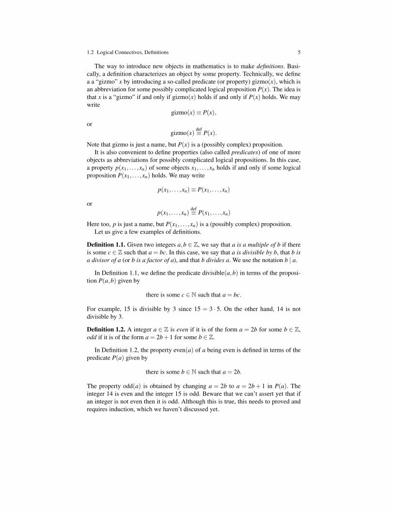
The way to introduce new objects in mathematics is to make definitions. Basi-cally, a definition characterizes an object by some property. Technically, we definea a “gizmo” x by introducing a so-called predicate (or property) gizmo(x), which isan abbreviation for some possibly complicated logical proposition P(x). The idea isthat x is a “gizmo” if and only if gizmo(x) holds if and only if P(x) holds. We maywrite
gizmo(x)≡ P(x),
orgizmo(x)
def≡ P(x).
Note that gizmo is just a name, but P(x) is a (possibly complex) proposition.It is also convenient to define properties (also called predicates) of one of more
objects as abbreviations for possibly complicated logical propositions. In this case,a property p(x1, . . . ,xn) of some objects x1, . . . ,xn holds if and only if some logicalproposition P(x1, . . . ,xn) holds. We may write
p(x1, . . . ,xn)≡ P(x1, . . . ,xn)
orp(x1, . . . ,xn)
def≡ P(x1, . . . ,xn)
Here too, p is just a name, but P(x1, . . . ,xn) is a (possibly complex) proposition.Let us give a few examples of definitions.
Definition 1.1. Given two integers a,b ∈ Z, we say that a is a multiple of b if thereis some c ∈ Z such that a = bc. In this case, we say that a is divisible by b, that b isa divisor of a (or b is a factor of a), and that b divides a. We use the notation b | a.
In Definition 1.1, we define the predicate divisible(a,b) in terms of the proposi-tion P(a,b) given by
there is some c ∈ N such that a = bc.
For example, 15 is divisible by 3 since 15 = 3 · 5. On the other hand, 14 is notdivisible by 3.
Definition 1.2. A integer a ∈ Z is even if it is of the form a = 2b for some b ∈ Z,odd if it is of the form a = 2b+1 for some b ∈ Z.
In Definition 1.2, the property even(a) of a being even is defined in terms of thepredicate P(a) given by
there is some b ∈ N such that a = 2b.
The property odd(a) is obtained by changing a = 2b to a = 2b+ 1 in P(a). Theinteger 14 is even and the integer 15 is odd. Beware that we can’t assert yet that ifan integer is not even then it is odd. Although this is true, this needs to proved andrequires induction, which we haven’t discussed yet.
6 1 Mathematical Reasoning And Basic Logic
Prime numbers play a fundamental role in mathematics. Let us review their defi-nition.
Definition 1.3. A natural number p ∈N is prime if p≥ 2 and if the only divisors ofp are 1 and p.
If we expand the definition of a prime number by replacing the predicate divisibleby its defining formula we get a rather complicated formula. Definitions allow us tobe more concise.
According to Definition 1.3, the number 1 is not prime even though it is onlydivisible by 1 and itself (again 1). The reason for not accepting 1 as a prime is notcapricious. It has to do with the fact that if we allowed 1 to be a prime, then certainimportant theorems (such as the unique prime factorization theorem, Theorem 7.10)would no longer hold.
Nonprime natural numbers (besides 1) have a special name too.
Definition 1.4. A natural number a ∈ N is composite if a = bc for some naturalnumbers b,c with b,c≥ 2.
For example, 4, 15, 36 are composite. Note that 1 is neither prime nor a compos-ite. We are now ready to introduce the proof tempates for implication.
1.3 Proof Templates for Implication
First, it is important to say that there are two types of proofs:
1. Direct proofs.2. Indirect proofs.
Indirect proofs use the proof–by–contradiction principle, which will be discussedsoon.
We begin by presenting proof templates to construct direct proofs of implications.An implication P⇒Q can be understood as an if–then statement; that is, if P is truethen Q is also true. A better interpretation is that any proof of P⇒Q can be used toconstruct a proof of Q given any proof of P. As a consequence of this interpretation,we show later that if ¬P is provable, then P⇒Q is also provable (instantly) whetheror not Q is provable. In such a situation, we often say that P⇒ Q is vacuouslyprovable. For example, (P∧¬P)⇒ Q is provable for any arbitrary Q.
During the process of constructing a proof, it may be necessary to introduce alist of hypotheses, also called premises (or assumptions), which grows and shrinksduring the proof. When a proof is finished, it should have an empty list of premises.
The process of managing the list of premises during a proof is a bit technical. InChapter 2, we study carefully two methods for managing the list of premises thatmay appear during a proof. In this chapter, we are much more casual about it, whichis the usual attitude when we write informal proofs. It suffices to be aware that at
1.3 Proof Templates for Implication 7
certain steps, some premises must be added, and at other special steps, premisesmust be discarded. We may view this as a process of making certain propositionsactive or inactive. To make matters clearer, we call the process of constructing aproof using a set of premises a deduction, and we reserve the word proof for adeduction whose set of premises is empty. Every deduction has a possibly emptylist of premises, and a single conclusion. The list of premises is usually denoted byΓ , and if the conclusion of the deduction is P, we say that we have a deduction of Pfrom the premises Γ .
The first proof template allows us to make obvious deductions.
Proof Template 1.1. (Trivial Deductions)
If P1, . . . ,Pi, . . . ,Pn is a list of propositions assumed as premises (where each Pi mayoccur more than once), then for each Pi, we have a deduction with conclusion Pi.
The second proof template allows the construction of a deduction whose conclu-sion is an implication P⇒ Q.
Proof Template 1.2. (Implication–Intro)
Given a list Γ of premises (possibly empty), to obtain a deduction with conclusionP⇒ Q, proceed as follows:
1. Add P as an additional premise to the list Γ .2. Make a deduction of the conclusion Q, from P and the premises in Γ .3. Delete P from the list of premises.
The third proof template allows the constructions of a deduction from two otherdeductions.
Proof Template 1.3. (Implication–Elim, or Modus–Ponens)
Given a deduction with conclusion P⇒ Q and a deduction with conclusion P, bothwith the same list Γ of premises, we obtain a deduction with conclusion Q. The listof premises of this new deduction is Γ .
Remark: In case you wonder why the words “Intro” and “Elim” occur in the namesassigned to the proof templates, the reason is the following:
1. If the proof template is tagged with X-intro, the connective X appears in theconclusion of the proof template; it is introduced. For example, in Proof Template1.2, the conclusion is P⇒ Q, and⇒ is indeed introduced.
2. If the proof template is tagged with X-Elim, the connective X appears in one ofthe premises of the proof template but it does not appear in the conclusion; it iseliminated. For example, in Proof Template 1.3 (modus ponens), P⇒ Q occursas a premise but the conclusion is Q; the symbol⇒ has been eliminated.
The introduction/elimination pattern is a characteristic of natural deduction proofsystems.

8 1 Mathematical Reasoning And Basic Logic
Example 1.1. Let us give a simple example of the use of Proof Template 1.2. Recallthat a natural number n is odd iff it is of the form 2k+1, where k ∈N. Let us denotethe fact that a number n is odd by odd(n). We would like to prove the implication
odd(n)⇒ odd(n+2).
Following Proof Template 1.2, we add odd(n) as a premise (which means thatwe take as proven the fact that n is odd) and we try to conclude that n+ 2 must beodd. However, to say that n is odd is to say that n = 2k+1 for some natural numberk. Now,
n+2 = 2k+1+2 = 2(k+1)+1,
which means that n+ 2 is odd. (Here, n = 2h+ 1, with h = k + 1, and k + 1 is anatural number because k is.)
Thus, we proved that if we assume odd(n), then we can conclude odd(n+2), andaccording to Proof Template 1.2, by step (3) we delete the premise odd(n) and weobtain a proof of the proposition
odd(n)⇒ odd(n+2).
It should be noted that the above proof of the proposition odd(n)⇒ odd(n+ 2)does not depend on any premises (other than the implicit fact that we are assuming nis a natural number). In particular, this proof does not depend on the premise odd(n),which was assumed (became “active”) during our subproof step. Thus, after havingapplied the Proof Template 1.2, we made sure that the premise odd(n) is deactivated.
Example 1.2. For a second example, we wish to prove the proposition P⇒ P.According to Proof Template 1.2, we assume P. But then, by Proof Template 1.1,
we obtain a deduction with premise P and conclusion P; by executing step (3) ofProof Template 1.2, the premise P is deleted, and we obtain a deduction of P⇒ Pfrom the empty list of premises. Thank God, P⇒ P is provable!
Proofs described in words as above are usually better understood when repre-sented as treees. We will reformulate our proof templates in tree form and explainvery precisely how to build proofs as trees in Chapter 2. For now, we use tree repre-sentations of proofs in an informal way.
A proof tree is drawn with its leaves at the top, corresponding to assumptions,and its root at the bottom, corresponding to the conclusion. In computer science,trees are usually drawn with their root at the top and their leaves at the bottom, butproof trees are drawn as the trees that we see in nature. Instead of linking nodes byedges, it is customary to use horizontal bars corresponding to the proof templates.One or more nodes appear as premises above a vertical bar, and the conclusion ofthe proof template appears immediately below the vertical bar.
The above proof of P⇒ P (presented in words) is represented by the tree shownbelow. Observe that the premise P is tagged with the symbol
√, which means that
it has been deleted from the list of premises. The tree representation of proofs alsohas the advantage that we can tag the premises in such a way that each tag indicateswhich rule causes the corresponding premise to be deleted. In the tree below, the
1.3 Proof Templates for Implication 9
premise P is tagged with x, and it is deleted when the proof template indicated by xis applied.
Px√
Trivial DeductionP Implication-Intro x
P⇒ P
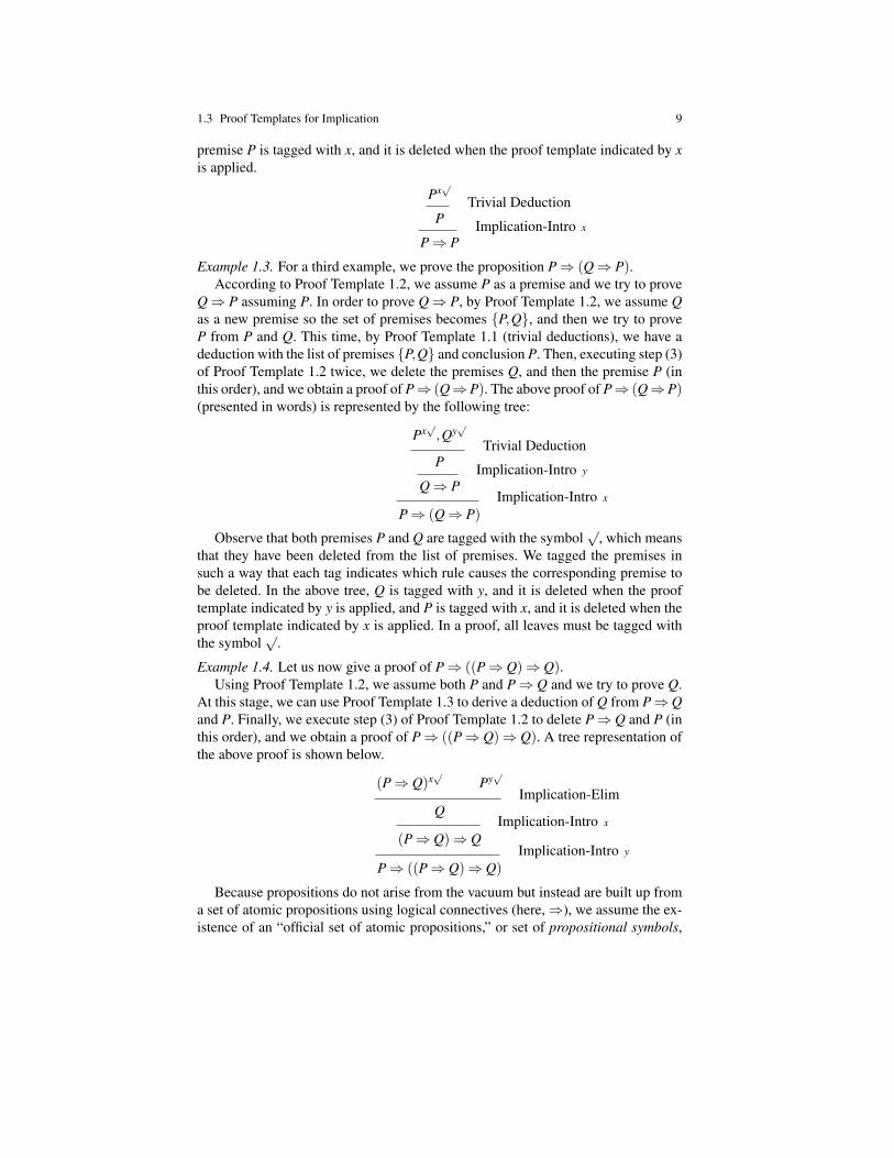
Example 1.3. For a third example, we prove the proposition P⇒ (Q⇒ P).According to Proof Template 1.2, we assume P as a premise and we try to prove
Q⇒ P assuming P. In order to prove Q⇒ P, by Proof Template 1.2, we assume Qas a new premise so the set of premises becomes P,Q, and then we try to proveP from P and Q. This time, by Proof Template 1.1 (trivial deductions), we have adeduction with the list of premises P,Q and conclusion P. Then, executing step (3)of Proof Template 1.2 twice, we delete the premises Q, and then the premise P (inthis order), and we obtain a proof of P⇒ (Q⇒P). The above proof of P⇒ (Q⇒P)(presented in words) is represented by the following tree:
Px√,Qy√
Trivial DeductionP Implication-Intro y
Q⇒ PImplication-Intro x
P⇒ (Q⇒ P)
Observe that both premises P and Q are tagged with the symbol√
, which meansthat they have been deleted from the list of premises. We tagged the premises insuch a way that each tag indicates which rule causes the corresponding premise tobe deleted. In the above tree, Q is tagged with y, and it is deleted when the prooftemplate indicated by y is applied, and P is tagged with x, and it is deleted when theproof template indicated by x is applied. In a proof, all leaves must be tagged withthe symbol
√.
Example 1.4. Let us now give a proof of P⇒ ((P⇒ Q)⇒ Q).Using Proof Template 1.2, we assume both P and P⇒ Q and we try to prove Q.
At this stage, we can use Proof Template 1.3 to derive a deduction of Q from P⇒Qand P. Finally, we execute step (3) of Proof Template 1.2 to delete P⇒Q and P (inthis order), and we obtain a proof of P⇒ ((P⇒ Q)⇒ Q). A tree representation ofthe above proof is shown below.
(P⇒ Q)x√
Py√
Implication-ElimQ
Implication-Intro x
(P⇒ Q)⇒ QImplication-Intro y
P⇒ ((P⇒ Q)⇒ Q)
Because propositions do not arise from the vacuum but instead are built up froma set of atomic propositions using logical connectives (here,⇒), we assume the ex-istence of an “official set of atomic propositions,” or set of propositional symbols,

10 1 Mathematical Reasoning And Basic Logic
PS = P1,P2,P3, . . .. So, for example, P1 ⇒ P2 and P1 ⇒ (P2 ⇒ P1) are propo-sitions. Typically, we use upper-case letters such as P,Q,R,S,A,B,C, and so on, todenote arbitrary propositions formed using atoms from PS.
It might help to view the action of proving an implication P⇒Q as the construc-tion of a program that converts a proof of P into a proof of Q. Then, if we supply aproof of P as input to this program (the proof of P⇒Q), it will output a proof of Q.So, if we don’t give the right kind of input to this program, for example, a “wrongproof” of P, we should not expect the program to return a proof of Q. However,this does not say that the program is incorrect; the program was designed to do theright thing only if it is given the right kind of input. From this functional point ofview (also called constructive), we should not be shocked that the provability of animplication P⇒ Q generally yields no information about the provability of Q.
For a concrete example, say P stands for the statement,“Our candidate for president wins in Pennsylvania”and Q stands for“Our candidate is elected president.”Then, P⇒ Q, asserts that if our candidate for president wins in Pennsylvania
then our candidate is elected president.If P⇒ Q holds, then if indeed our candidate for president wins in Pennsylvania
then for sure our candidate will win the presidential election. However, if our candi-date does not win in Pennsylvania, we can’t predict what will happen. Our candidatemay still win the presidential election but he may not.
If our candidate president does not win in Pennsylvania, then the statement P⇒Q should be regarded as holding, though perhaps uninteresting.
For one more example, let odd(n) assert that n is an odd natural number and letQ(n,a,b) assert that an + bn is divisible by a+ b, where a,b are any given naturalnumbers. By divisible, we mean that we can find some natural number c, so that
an +bn = (a+b)c.
Then, we claim that the implication odd(n)⇒ Q(n,a,b) is provable.As usual, let us assume odd(n), so that n = 2k+ 1, where k = 0,1,2,3, . . .. But
then, we can easily check that
a2k+1 +b2k+1 = (a+b)
(2k
∑i=0
(−1)ia2k−ibi
),
which shows that a2k+1 +b2k+1 is divisible by a+b. Therefore, we proved the im-plication odd(n)⇒ Q(n,a,b).
If n is not odd, then the implication odd(n)⇒ Q(n,a,b) yields no informationabout the provablity of the statement Q(n,a,b), and that is fine. Indeed, if n is evenand n≥ 2, then in general, an +bn is not divisible by a+b, but this may happen forsome special values of n, a, and b, for example: n = 2, a = 2, b = 2.

1.4 Proof Templates for ¬,∧,∨,≡ 11
Beware, when we deduce that an implication P⇒ Q is provable, we do notprove that P and Q are provable; we only prove that if P is provable then Q is
provable.
The modus–ponens proof template formalizes the use of auxiliary lemmas, amechanism that we use all the time in making mathematical proofs. Think of P⇒Q as a lemma that has already been established and belongs to some database of(useful) lemmas. This lemma says if I can prove P then I can prove Q. Now, supposethat we manage to give a proof of P. It follows from modus–ponens that Q is alsoprovable.
Mathematicians are very fond of modus–ponens because it gives a potentialmethod for proving important results. If Q is an important result and if we man-age to build a large catalog of implications P⇒ Q, there may be some hope that,some day, P will be proved, in which case Q will also be proved. So, they build largecatalogs of implications! This has been going on for the famous problem known asP versus NP. So far, no proof of any premise of such an implication involving Pversus NP has been found (and it may never be found).
Remark: We have not yet examined how we how we can represent precisely arbi-trary deductions. This can be done using certain types of trees where the nodes aretagged with lists of premises. Two methods for doing this are carefully defined inChapter 2. It turns out that the same premise may be used in more than one locationin the tree, but in our informal presentation, we ignore such fine details.
We now describe the proof templates dealing with the connectives ¬,∧,∨,≡.
1.4 Proof Templates for ¬,∧,∨,≡
Recall that ¬P is an abbreviation for P⇒⊥. We begin with the proof templates fornegation, for direct proofs.
Proof Template 1.4. (Negation–Intro)
Given a list Γ of premises (possibly empty), to obtain a deduction with conclusion¬P, proceed as follows:
1. Add P as an additional premise to the list Γ .2. Derive a contradiction. More precisely, make a deduction of the conclusion ⊥
from P and the premises in Γ .3. Delete P from the list of premises.
Proof Template 1.4 is a special case of Proof Template 1.2, since ¬P is an abbre-viation for P⇒⊥.
Proof Template 1.5. (Negation–Elim)
Given a deduction with conclusion ¬P and a deduction with conclusion P, bothwith the same list Γ of premises, we obtain a contradiction; that is, a deduction withconclusion ⊥. The list of premises of this new deduction is Γ .

12 1 Mathematical Reasoning And Basic Logic
Proof Template 1.5 is a special case of Proof Template 1.3, since ¬P is an abbre-viation for P⇒⊥.
Proof Template 1.6. (Perp–Elim)
Given a deduction with conclusion ⊥ (a contradiction), for every proposition Q, weobtain a deduction with conclusion Q. The list of premises of this new deduction isthe same as the original list of premises.
The last proof template for negation constructs an indirect proof; it is the proof–by–contradiction principle.
Proof Template 1.7. (Proof–By–Contradiction Principle)
Given a list Γ of premises (possibly empty), to obtain a deduction with conclusionP, proceed as follows:
1. Add ¬P as an additional premise to the list Γ .2. Derive a contradiction. More precisely, make a deduction of the conclusion ⊥
from ¬P and the premises in Γ .3. Delete ¬P from the list of premises.
Proof Template 1.7 (the proof–by–contradiction principle) also has the fancyname of reductio ad absurdum rule, for short RAA.
Proof Template 1.6 may seem silly and one might wonder why we stated it. Itturns out that it is subsumed by Proof Template 1.7, but it is still useful to state it asa proof template. Let us give an example showing how it is used.
Example 1.5. Let us prove that (¬(P⇒ Q))⇒ P.First, we use Proof Template 1.2, and we assume ¬(P⇒ Q) as a premise. Next,
we use the proof–by–contradiction principle (Proof Template 1.7). So, in order toprove P, we assume ¬P as another premise. The next step is to deduce P⇒ Q.By Proof Template 1.2, we assume P as an additional premise. By Proof Template1.5, from ¬P and P we obtain a deduction of ⊥, and then by Proof Template 1.6a deduction of Q from ¬P and P. By Proof Template 1.2, executing step (3), wedelete the premise P and we obtain a deduction of P⇒ Q. At this stage, we havethe premises ¬P,¬(P⇒ Q) and a deduction of P⇒ Q, so by Proof Template 1.5,we obtain a deduction of ⊥. This is a contradiction, so by step (3) of the proof–by–contradiction principle (Proof Template 1.7) we can delete the premise ¬P, andwe have a deduction of P from ¬(P⇒ Q). Finally, we execute step (3) of ProofTemplate 1.2 and delete the premise ¬(P⇒ Q), which yields the desired proof of(¬(P⇒ Q))⇒ P. The above proof has the following tree representation.

1.4 Proof Templates for ¬,∧,∨,≡ 13
¬(P⇒ Q)z√
¬Py√
Px√
⊥Q
x
P⇒ Q
⊥y
Pz
(¬(P⇒ Q))⇒ P
The reader may be surprised by how many steps are needed in the above proofand may wonder whether the proof–by–contradiction principle is actually needed.It can be shown that the proof–by–contradiction principle must be used, and unfor-tuately there is no shorter proof.
Example 1.6. Let us now prove that (¬(P⇒ Q))⇒¬Q.First, by Proof Template 1.2, we add ¬(P⇒ Q) as a premise. Then, in order to
prove ¬Q from ¬(P⇒ Q), we use Proof Template 1.4 and we add Q as a premise.Now, recall that we showed in Example 1.3 that P⇒Q is provable assuming Q (withP and Q switched). Then, since ¬(P⇒ Q) is a premise, by Proof Template 1.5, weobtain a deduction of ⊥. We now execute step (3) of Proof Template 1.4, delete thepremise Q to obtain a deduction of ¬Q from ¬(P⇒ Q), we and we execute step(3) of Proof Template 1.2 to delete the premise ¬(P⇒ Q) and obtain a proof of(¬(P⇒ Q))⇒¬Q. The above proof corresponds to the following tree.
¬(P⇒ Q)z√
Qy√
Px√
Qx
P⇒ Q
⊥y
¬Qz
(¬(P⇒ Q))⇒¬Q
Example 1.7. Let us prove that for every natural number n, if n2 is odd, then n itselfmust be odd.
We use the proof–by–contradiction principle (Proof Template 1.7), so we assumethat n is not odd, which means that n is even. (Actually, in this step we are using aproperty of the natural numbers that is proved by induction but let’s not worry aboutthat right now; a proof can be found in Section 1.10) But to say that n is even meansthat n = 2k for some k and then n2 = 4k2 = 2(2k2), so n2 is even, contradicting theassumption that n2 is odd. By the proof–by–contradiction principle (Proof Template1.7), we conclude that n must be odd.
Example 1.8. Let us prove that ¬¬P⇒ P.
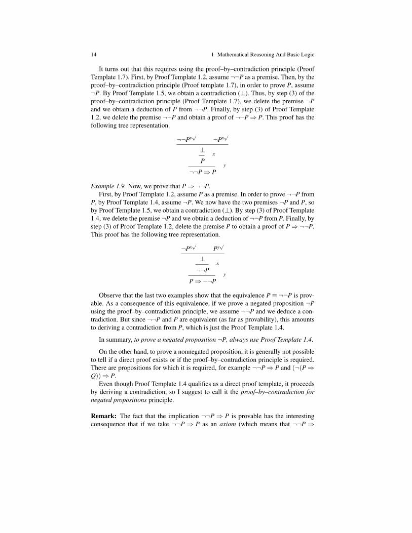
14 1 Mathematical Reasoning And Basic Logic
It turns out that this requires using the proof–by–contradiction principle (ProofTemplate 1.7). First, by Proof Template 1.2, assume ¬¬P as a premise. Then, by theproof–by–contradiction principle (Proof template 1.7), in order to prove P, assume¬P. By Proof Template 1.5, we obtain a contradiction (⊥). Thus, by step (3) of theproof–by–contradiction principle (Proof Template 1.7), we delete the premise ¬Pand we obtain a deduction of P from ¬¬P. Finally, by step (3) of Proof Template1.2, we delete the premise ¬¬P and obtain a proof of ¬¬P⇒ P. This proof has thefollowing tree representation.
¬¬Py√
¬Px√
⊥x
Py
¬¬P⇒ P
Example 1.9. Now, we prove that P⇒¬¬P.First, by Proof Template 1.2, assume P as a premise. In order to prove ¬¬P from
P, by Proof Template 1.4, assume ¬P. We now have the two premises ¬P and P, soby Proof Template 1.5, we obtain a contradiction (⊥). By step (3) of Proof Template1.4, we delete the premise ¬P and we obtain a deduction of ¬¬P from P. Finally, bystep (3) of Proof Template 1.2, delete the premise P to obtain a proof of P⇒¬¬P.This proof has the following tree representation.
¬Px√
Py√
⊥x
¬¬Py
P⇒¬¬P
Observe that the last two examples show that the equivalence P ≡ ¬¬P is prov-able. As a consequence of this equivalence, if we prove a negated proposition ¬Pusing the proof–by–contradiction principle, we assume ¬¬P and we deduce a con-tradiction. But since ¬¬P and P are equivalent (as far as provability), this amountsto deriving a contradiction from P, which is just the Proof Template 1.4.
In summary, to prove a negated proposition ¬P, always use Proof Template 1.4.
On the other hand, to prove a nonnegated proposition, it is generally not possibleto tell if a direct proof exists or if the proof–by–contradiction principle is required.There are propositions for which it is required, for example ¬¬P⇒ P and (¬(P⇒Q))⇒ P.
Even though Proof Template 1.4 qualifies as a direct proof template, it proceedsby deriving a contradiction, so I suggest to call it the proof–by–contradiction fornegated propositions principle.
Remark: The fact that the implication ¬¬P⇒ P is provable has the interestingconsequence that if we take ¬¬P ⇒ P as an axiom (which means that ¬¬P ⇒
1.4 Proof Templates for ¬,∧,∨,≡ 15
P is assumed to be provable without requiring any proof), then the proof–by–contradiction principle (Proof Template 1.7) becomes redundant. Indeed, ProofTemplate 1.7 is subsumed by Proof Template 1.4, because if we have a deductionof ⊥ from ¬P, then by Proof Template 1.4 we delete the premise ¬P to obtain adeduction of ¬¬P. Since ¬¬P⇒ P is assumed to be provable, by Proof Template1.3, we get a proof of P. The tree shown below illustrates what is going on. In thistree, a proof of ⊥ from the premise ¬P is denoted by D .
¬¬P⇒ P
¬Px√
D
⊥x
¬¬PP
Proof Templates 1.5 and 1.6 together imply that if a contradiction is obtained dur-ing a deduction because two inconsistent propositions P and ¬P are obtained, thenall propositions are provable (anything goes). This explains why mathematicians areleary of inconsistencies.
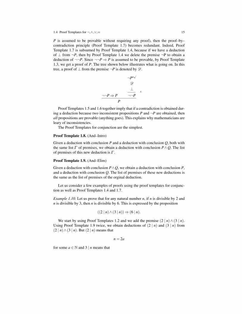
The Proof Templates for conjunction are the simplest.
Proof Template 1.8. (And–Intro)
Given a deduction with conclusion P and a deduction with conclusion Q, both withthe same list Γ of premises, we obtain a deduction with conclusion P∧Q. The listof premises of this new deduction is Γ .
Proof Template 1.9. (And–Elim)
Given a deduction with conclusion P∧Q, we obtain a deduction with conclusion P,and a deduction with conclusion Q. The list of premises of these new deductions isthe same as the list of premises of the orginal deduction.
Let us consider a few examples of proofs using the proof templates for conjunc-tion as well as Proof Templates 1.4 and 1.7.
Example 1.10. Let us prove that for any natural number n, if n is divisible by 2 andn is divisible by 3, then n is divisible by 6. This is expressed by the proposition
((2 | n)∧ (3 | n))⇒ (6 | n).
We start by using Proof Templates 1.2 and we add the premise (2 | n)∧ (3 | n).Using Proof Template 1.9 twice, we obtain deductions of (2 | n) and (3 | n) from(2 | n)∧ (3 | n). But (2 | n) means that
n = 2a
for some a ∈ N and 3 | n means that

16 1 Mathematical Reasoning And Basic Logic
n = 3b
for some b ∈ N. This implies that
n = 2a = 3b.
Because 2 and 3 are relatively prime (their only common divisor is 1), the number2 must divide b (and 3 must divide a) so b = 2c for some c ∈ N. Here we are usingEuclid’s lemma, see Proposition 7.9. So, we have shown that
n = 3b = 3 ·2c = 6c,
which says that n is divisible by 6. We conclude with step (3) of Proof Template 1.2by deleting the premise (2 | n)∧ (3 | n) and we obtain our proof.
Example 1.11. Let us prove that for any natural number n, if n is divisible by 6, thenn is divisible by 2 and n is divisible by 3. This is expressed by the proposition
(6 | n)⇒ ((2 | n)∧ (3 | n)).
We start by using Proof Templates 1.2 and we add the premise 6 | n. This meansthat
n = 6a = 2 ·3a
for some a∈N. This implies that 2 | n and 3 | n, so we have a deduction of 2 | n fromthe premise 6 | n and a deduction of 3 | n from the premise 6 | n. By Proof Template1.8, we obtain a deduction of (2 | n)∧ (3 | n) from 6 | n, and we apply step (3) ofProof Template 1.2 to delete the premise 6 | n and obtain our proof.
Example 1.12. Let us prove that (¬(P⇒ Q))⇒ (P∧¬Q).We start by using Proof Templates 1.2 and we add ¬(P ⇒ Q) as a premise.
Now, in Example 1.5 we showed that (¬(P⇒ Q))⇒ P is provable, and this proofcontains a deduction of P from ¬(P⇒ Q). Similarly, in Example 1.6 we showedthat (¬(P⇒ Q))⇒ ¬Q is provable, and this proof contains a deduction of ¬Qfrom ¬(P⇒ Q). By proof Template 1.8, we obtain a deduction of P∧¬Q from¬(P⇒ Q), and executing step (3) of Proof Templates 1.2, we obtain a proof of(¬(P⇒ Q))⇒ (P∧¬Q). The following tree represents the above proof. Observethat two copies of the premise ¬(P⇒ Q) are needed.
1.4 Proof Templates for ¬,∧,∨,≡ 17
¬(P⇒ Q)z√
¬Py√
Px√
⊥Q
x
P⇒ Q
⊥y
P
¬(P⇒ Q)z√
Qw√
Pt√
Qt
P⇒ Q
⊥w
¬Q
P∧¬Qz
(¬(P⇒ Q))⇒ (P∧¬Q)
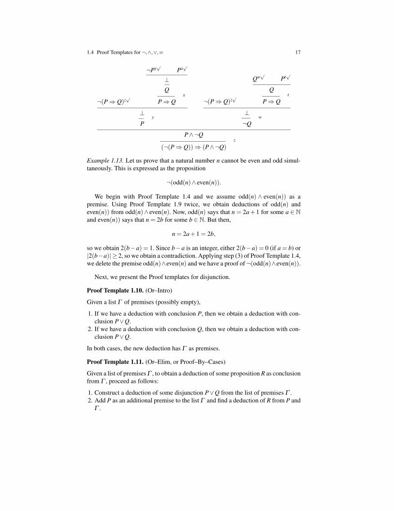
Example 1.13. Let us prove that a natural number n cannot be even and odd simul-taneously. This is expressed as the proposition
¬(odd(n)∧ even(n)).
We begin with Proof Template 1.4 and we assume odd(n) ∧ even(n)) as apremise. Using Proof Template 1.9 twice, we obtain deductions of odd(n) andeven(n)) from odd(n)∧ even(n). Now, odd(n) says that n = 2a+1 for some a ∈ Nand even(n)) says that n = 2b for some b ∈ N. But then,
n = 2a+1 = 2b,
so we obtain 2(b−a) = 1. Since b−a is an integer, either 2(b−a) = 0 (if a = b) or|2(b−a)| ≥ 2, so we obtain a contradiction. Applying step (3) of Proof Template 1.4,we delete the premise odd(n)∧even(n) and we have a proof of ¬(odd(n)∧even(n)).
Next, we present the Proof templates for disjunction.
Proof Template 1.10. (Or–Intro)
Given a list Γ of premises (possibly empty),
1. If we have a deduction with conclusion P, then we obtain a deduction with con-clusion P∨Q.
2. If we have a deduction with conclusion Q, then we obtain a deduction with con-clusion P∨Q.
In both cases, the new deduction has Γ as premises.
Proof Template 1.11. (Or–Elim, or Proof–By–Cases)
Given a list of premises Γ , to obtain a deduction of some proposition R as conclusionfrom Γ , proceed as follows:
1. Construct a deduction of some disjunction P∨Q from the list of premises Γ .2. Add P as an additional premise to the list Γ and find a deduction of R from P and
Γ .

18 1 Mathematical Reasoning And Basic Logic
3. Add Q as an additional premise to the list Γ and find a deduction of R from Qand Γ .
Note that in making the two deductions of R, the premise P∨Q is not assumed.Proof Template 1.10 may seem trivial, so let us show an example illustrating its
use.
Example 1.14. Let us prove that ¬(P∨Q)⇒ (¬P∧¬Q).First, by Proof Template 1.2, we assume ¬(P∨Q) (two copies). In order to derive
¬P, by Proof Template 1.4, we also assume P. Then by Proof Template 1.10 wededuce P∨Q, and since we have the premise ¬(P∨Q), by Proof Template 1.5 weobtain a contradiction. By Proof Template 1.4, we can delete the premise P andobtain a deduction of ¬P from ¬(P∨Q).
In a similar way we can construct a deduction of ¬Q from ¬(P∨Q). By ProofTemplate 1.8, we get a deduction of ¬P∧¬Q from ¬(P∨Q), and we finish byapplying Proof Template 1.2. A tree representing the above proof is shown below.
¬(P∨Q)z√
Px√
P∨Q
⊥x
¬P
¬(P∨Q)z√
Qw√
P∨Q
⊥w
¬Q
¬P∧¬Qz
¬(P∨Q)⇒ (¬P∧¬Q)
The proposition (¬P∧¬Q)⇒ ¬(P∨Q) is also provable using the proof–by–cases principle. Here is a proof tree; we leave it as an exercise to the reader to checkthat the proof templates have been applied correctly.
(P∨Q)z√
(¬P∧¬Q)t√
¬P Px√
⊥
(¬P∧¬Q)t√
¬Q Qy√
⊥x,y
⊥z
¬(P∨Q)t
(¬P∧¬Q)⇒¬(P∨Q)
As a consequence the equivalence
¬(P∨Q)≡ (¬P∧¬Q)
is provable. This is one of three identities known as de Morgan laws.
Example 1.15. Next, let us prove that ¬(¬P∨¬Q)⇒ P.

1.4 Proof Templates for ¬,∧,∨,≡ 19
First, by Proof Template 1.2, we assume ¬(¬P∨¬Q) as a premise. In order toprove P from¬(¬P∨¬Q), we use the proof–by–contradiction principle (Proof Tem-plate 1.7). So, we add ¬P as a premise. Now, by Proof Template 1.10, we can de-duce ¬P∨¬Q from ¬P, and since ¬(¬P∨¬Q) is a premise, by Proof Template 1.5,we obtain a contradiction. By the proof–by–contradiction principle (Proof Template1.7), we delete the premise ¬P and we obtain a deduction of P from ¬(¬P∨¬Q).We conclude by using Proof Template 1.2 to delete the premise ¬(¬P∨¬Q) and toobtain our proof. A tree representing the above proof is shown below.
¬(¬P∨¬Q)y√
¬Px√
¬P∨¬Q
⊥x
Py
¬(¬P∨¬Q)⇒ P
A similar proof shows that ¬(¬P∨¬Q)⇒ Q is provable. Putting together theproofs of P and Q from ¬(¬P∨¬Q) using Proof Template 1.8, we obtain a proof of
¬(¬P∨¬Q)⇒ (P∧Q).
A tree representing this proof is shown below.
¬(¬P∨¬Q)y√
¬Px√
¬P∨¬Q
⊥x
P
¬(¬P∨¬Q)y√
¬Qw√
¬P∨¬Q
⊥w
Q
P∧Qy
¬(¬P∨¬Q)⇒ (P∧Q)
Example 1.16. The proposition ¬(P∧Q)⇒ (¬P∨¬Q) is provable.First, by Proof Template 1.2, we assume ¬(P∧Q) as a premise. Next, we use
the proof–by–contradiction principle (Proof Template 1.7) to deduce ¬P∨¬Q, sowe also assume ¬(¬P∨¬Q). Now, we just showed that P∧Q is provable from thepremise ¬(¬P∨¬Q). Using the premise ¬(P∧Q), by Proof Principle 1.5, we derivea contradiction, and by the proof–by–contradiction principle, we delete the premise¬(¬P∨¬Q) to obtain a deduction of ¬P∨¬Q from ¬(P∧Q). We finish the proofby Applying Proof Template 1.2. This proof is represented by the following tree.
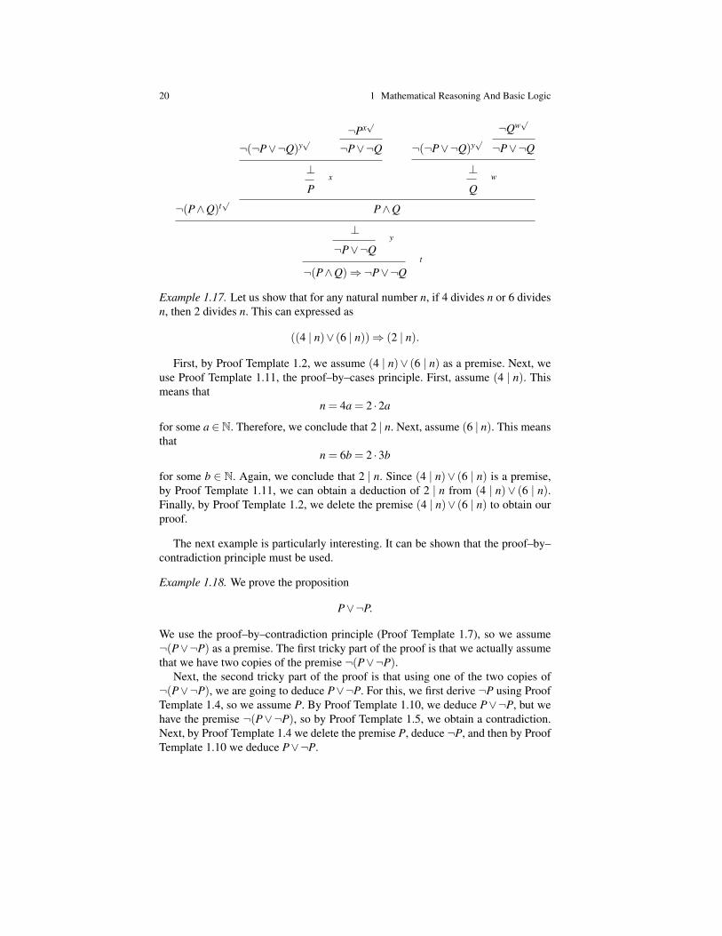
20 1 Mathematical Reasoning And Basic Logic
¬(P∧Q)t√
¬(¬P∨¬Q)y√
¬Px√
¬P∨¬Q
⊥x
P
¬(¬P∨¬Q)y√¬Qw
√
¬P∨¬Q
⊥w
Q
P∧Q
⊥y
¬P∨¬Qt
¬(P∧Q)⇒¬P∨¬Q
Example 1.17. Let us show that for any natural number n, if 4 divides n or 6 dividesn, then 2 divides n. This can expressed as
((4 | n)∨ (6 | n))⇒ (2 | n).
First, by Proof Template 1.2, we assume (4 | n)∨ (6 | n) as a premise. Next, weuse Proof Template 1.11, the proof–by–cases principle. First, assume (4 | n). Thismeans that
n = 4a = 2 ·2a
for some a ∈N. Therefore, we conclude that 2 | n. Next, assume (6 | n). This meansthat
n = 6b = 2 ·3b
for some b ∈ N. Again, we conclude that 2 | n. Since (4 | n)∨ (6 | n) is a premise,by Proof Template 1.11, we can obtain a deduction of 2 | n from (4 | n)∨ (6 | n).Finally, by Proof Template 1.2, we delete the premise (4 | n)∨ (6 | n) to obtain ourproof.
The next example is particularly interesting. It can be shown that the proof–by–contradiction principle must be used.
Example 1.18. We prove the proposition
P∨¬P.
We use the proof–by–contradiction principle (Proof Template 1.7), so we assume¬(P∨¬P) as a premise. The first tricky part of the proof is that we actually assumethat we have two copies of the premise ¬(P∨¬P).
Next, the second tricky part of the proof is that using one of the two copies of¬(P∨¬P), we are going to deduce P∨¬P. For this, we first derive ¬P using ProofTemplate 1.4, so we assume P. By Proof Template 1.10, we deduce P∨¬P, but wehave the premise ¬(P∨¬P), so by Proof Template 1.5, we obtain a contradiction.Next, by Proof Template 1.4 we delete the premise P, deduce ¬P, and then by ProofTemplate 1.10 we deduce P∨¬P.
1.4 Proof Templates for ¬,∧,∨,≡ 21
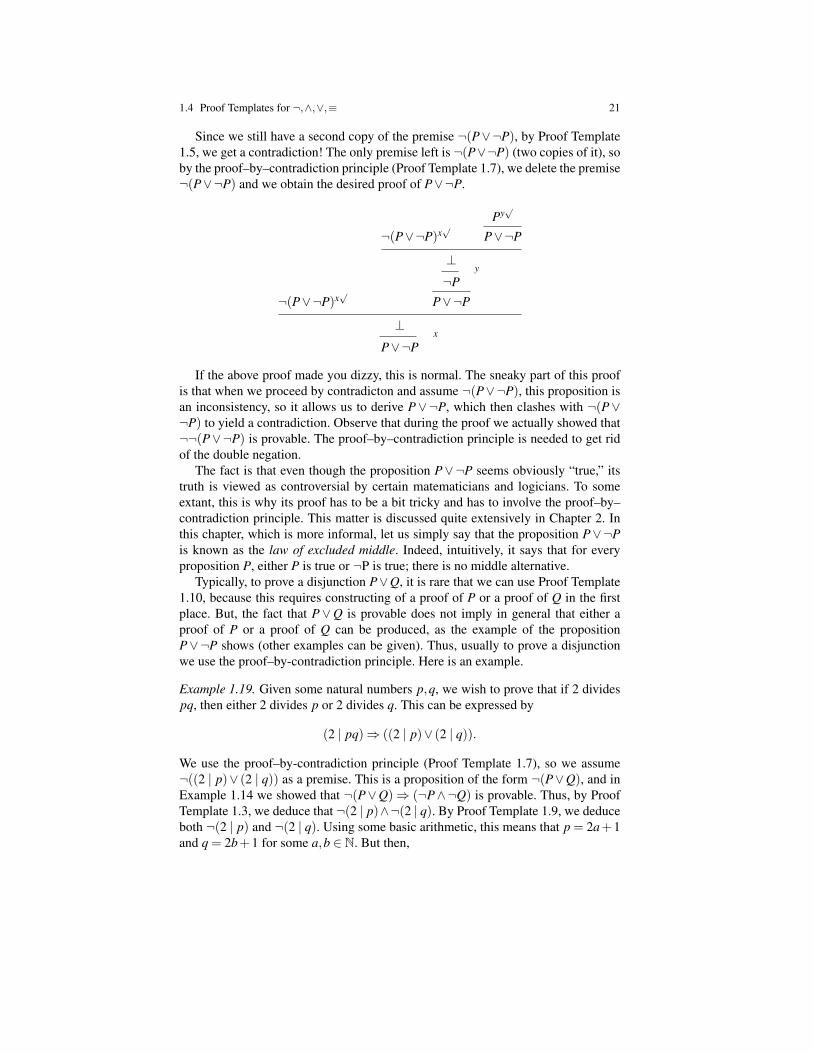
Since we still have a second copy of the premise ¬(P∨¬P), by Proof Template1.5, we get a contradiction! The only premise left is ¬(P∨¬P) (two copies of it), soby the proof–by–contradiction principle (Proof Template 1.7), we delete the premise¬(P∨¬P) and we obtain the desired proof of P∨¬P.
¬(P∨¬P)x√
¬(P∨¬P)x√
Py√
P∨¬P
⊥y
¬PP∨¬P
⊥x
P∨¬P
If the above proof made you dizzy, this is normal. The sneaky part of this proofis that when we proceed by contradicton and assume ¬(P∨¬P), this proposition isan inconsistency, so it allows us to derive P∨¬P, which then clashes with ¬(P∨¬P) to yield a contradiction. Observe that during the proof we actually showed that¬¬(P∨¬P) is provable. The proof–by–contradiction principle is needed to get ridof the double negation.
The fact is that even though the proposition P∨¬P seems obviously “true,” itstruth is viewed as controversial by certain matematicians and logicians. To someextant, this is why its proof has to be a bit tricky and has to involve the proof–by–contradiction principle. This matter is discussed quite extensively in Chapter 2. Inthis chapter, which is more informal, let us simply say that the proposition P∨¬Pis known as the law of excluded middle. Indeed, intuitively, it says that for everyproposition P, either P is true or ¬P is true; there is no middle alternative.
Typically, to prove a disjunction P∨Q, it is rare that we can use Proof Template1.10, because this requires constructing of a proof of P or a proof of Q in the firstplace. But, the fact that P∨Q is provable does not imply in general that either aproof of P or a proof of Q can be produced, as the example of the propositionP∨¬P shows (other examples can be given). Thus, usually to prove a disjunctionwe use the proof–by-contradiction principle. Here is an example.
Example 1.19. Given some natural numbers p,q, we wish to prove that if 2 dividespq, then either 2 divides p or 2 divides q. This can be expressed by
(2 | pq)⇒ ((2 | p)∨ (2 | q)).
We use the proof–by-contradiction principle (Proof Template 1.7), so we assume¬((2 | p)∨ (2 | q)) as a premise. This is a proposition of the form ¬(P∨Q), and inExample 1.14 we showed that ¬(P∨Q)⇒ (¬P∧¬Q) is provable. Thus, by ProofTemplate 1.3, we deduce that ¬(2 | p)∧¬(2 | q). By Proof Template 1.9, we deduceboth ¬(2 | p) and ¬(2 | q). Using some basic arithmetic, this means that p = 2a+1and q = 2b+1 for some a,b ∈ N. But then,

22 1 Mathematical Reasoning And Basic Logic
pq = 2(2ab+a+b)+1.
and pq is not divisible by 2, a contradiction. By the proof–by-contradiction principle(Proof Template 1.7), we can delete the premise ¬((2 | p)∨ (2 | q)) and obtain thedesired proof.
Another Proof Template which is convenient to use in some cases is the proof–by–contrapositive principle.
Proof Template 1.12. (Proof–By–Contrapositive)
Given a list of premises Γ , to prove an implication P⇒ Q, proceed as follows:
1. Add ¬Q to the list of premises Γ .2. Construct a deduction of ¬P from the premises ¬Q and Γ .3. Delete ¬Q from the list of premises.
It is not hard to see that the proof–by–contrapositive principle (Proof Template1.12) can be derived from the proof–by–contradiction principle. We leave this as anexercise.
Example 1.20. We prove that for any two natural numbers m,n∈N, if m+n is even,then m and n have the same parity. This can be expressed as
even(m+n)⇒ ((even(m)∧ even(n))∨ (odd(m)∧odd(n))).
According to Proof Template 1.12 (proof–by–contrapositive principle), let us as-sume ¬((even(m)∧even(n))∨(odd(m)∧odd(n))). Using the implication proved inExample 1.14 ((¬(P∨Q))⇒ ¬P∧¬Q)) and Proof Template 1.3, we deduce that¬(even(m)∧ even(n)) and ¬(odd(m)∧ odd(n)). Using the result of Example 1.16and modus ponens (Proof Template 1.3), we deduce that ¬even(m)∨¬even(n) and¬odd(m)∨¬odd(n). At this point, we can use the proof–by–cases principle (twice)to deduce that ¬even(m+n) holds. We leave some of the tedious details as an exer-cise. In particular, we use the fact proved in Chapter 2 that even(p) iff ¬odd(p) (seeSection 2.10).
We treat logical equivalence as a derived connective: that is, we view P ≡ Q asan abbreviation for (P⇒Q)∧(Q⇒ P). In view of the proof templates for ∧, we seethat to prove a logical equivalence P ≡ Q, we just have to prove both implicationsP⇒ Q and Q⇒ P. For the sake of completeness, we state the following prooftemplate.
Proof Template 1.13. (Equivalence–Intro)
Given a list of premises Γ , to obtain a deduction of an equivalence P≡ Q, proceedas follows:
1. Construct a deduction of the implication P⇒ Q from the list of premises Γ .2. Construct a deduction of the implication Q⇒ P from the list of premises Γ .
1.5 De Morgan Laws and Other Useful Rules of Logic 23
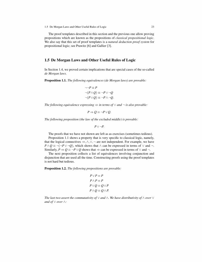
The proof templates described in this section and the previous one allow provingpropositions which are known as the propositions of classical propositional logic.We also say that this set of proof templates is a natural deduction proof system forpropositional logic; see Prawitz [6] and Gallier [3].
1.5 De Morgan Laws and Other Useful Rules of Logic
In Section 1.4, we proved certain implications that are special cases of the so-calledde Morgan laws.
Proposition 1.1. The following equivalences (de Morgan laws) are provable:
¬¬P≡ P
¬(P∧Q)≡ ¬P∨¬Q
¬(P∨Q)≡ ¬P∧¬Q.
The following equivalence expressing⇒ in terms of ∨ and ¬ is also provable:
P⇒ Q≡ ¬P∨Q.
The following proposition (the law of the excluded middle) is provable:
P∨¬P.
The proofs that we have not shown are left as as exercises (sometimes tedious).Proposition 1.1 shows a property that is very specific to classical logic, namely,
that the logical connectives ⇒,∧,∨,¬ are not independent. For example, we haveP∧Q ≡ ¬(¬P∨¬Q), which shows that ∧ can be expressed in terms of ∨ and ¬.Similarly, P⇒ Q≡ ¬P∨Q shows that⇒ can be expressed in terms of ∨ and ¬.
The next proposition collects a list of equivalences involving conjunction anddisjunction that are used all the time. Constructing proofs using the proof templatesis not hard but tedious.
Proposition 1.2. The following propositions are provable:
P∨P≡ P
P∧P≡ P
P∨Q≡ Q∨P
P∧Q≡ Q∧P.
The last two assert the commutativity of ∨ and ∧. We have distributivity of ∧ over ∨and of ∨ over ∧:
24 1 Mathematical Reasoning And Basic Logic
P∧ (Q∨R)≡ (P∧Q)∨ (P∧R)
P∨ (Q∧R)≡ (P∨Q)∧ (P∨R).
We have associativity of ∧ and ∨:
P∧ (Q∧R)≡ (P∧Q)∧R
P∨ (Q∨R)≡ (P∨Q)∨R.
1.6 Formal Versus Informal Proofs; Some Examples
In this section, we give some explicit examples of proofs illustrating the proof tem-plates that we just discussed. But first, it should be said that it is practically im-possible to write formal proofs (i.e., proofs written using the proof templates of thesystem presented earlier) of “real” statements that are not “toy propositions.” Thisis because it would be extremely tedious and time-consuming to write such proofsand these proofs would be huge and thus very hard to read.
As we said before it is possible in principle to write formalized proofs, however,most of us will never do so. So, what do we do?
Well, we construct “informal” proofs in which we still make use of the prooftemplates that we have presented but we take shortcuts and sometimes we evenomit proof steps (some proof templates such as 1.9 and 1.10) and we use a naturallanguage (here, presumably, English) rather than formal symbols (we say “and” for∧, “or” for ∨, etc.). As an example of a shortcut, when using the proof template1.11, in most cases, the disjunction P∨Q has an “obvious proof” because P and Q“exhaust all the cases,” in the sense that Q subsumes ¬P (or P subsumes ¬Q) andclassically, P∨¬P is an axiom. Also, we implicitly keep track of the open premisesof a proof in our head rather than explicitly delete premises when required. Thismay be the biggest source of mistakes and we should make sure that when we havefinished a proof, there are no “dangling premises,” that is, premises that were neverused in constructing the proof. If we are “lucky,” some of these premises are infact unnecessary and we should discard them. Otherwise, this indicates that thereis something wrong with our proof and we should make sure that every premise isindeed used somewhere in the proof or else look for a counterexample.
We urge our readers to read Chapter 3 of Gowers [10] which contains very illu-minating remarks about the notion of proof in mathematics.
The next question is then, “How does one write good informal proofs?”It is very hard to answer such a question because the notion of a “good” proof is
quite subjective and partly a social concept. Nevertheless, people have been writinginformal proofs for centuries so there are at least many examples of what to do(and what not to do). As with everything else, practicing a sport, playing a musicinstrument, knowing “good” wines, and so on, the more you practice, the better youbecome. Knowing the theory of swimming is fine but you have to get wet and do
1.6 Formal Versus Informal Proofs; Some Examples 25
some actual swimming. Similarly, knowing the proof rules is important but you haveto put them to use.
Write proofs as much as you can. Find good proof writers (like good swimmers,good tennis players, etc.), try to figure out why they write clear and easily readableproofs and try to emulate what they do. Don’t follow bad examples (it will take youa little while to “smell” a bad proof style).
Another important point is that nonformalized proofs make heavy use of modusponens. This is because, when we search for a proof, we rarely (if ever) go back tofirst principles. This would result in extremely long proofs that would be basicallyincomprehensible. Instead, we search in our “database” of facts for a propositionof the form P⇒ Q (an auxiliary lemma) that is already known to be proved, andif we are smart enough (lucky enough), we find that we can prove P and thus wededuce Q, the proposition that we really need to prove. Generally, we have to gothrough several steps involving auxiliary lemmas. This is why it is important tobuild up a database of proven facts as large as possible about a mathematical field:numbers, trees, graphs, surfaces, and so on. This way, we increase the chance thatwe will be able to prove some fact about some field of mathematics. On the otherhand, one might argue that it might be better to start fresh and not to know muchabout a problem in order to tackle it. Somehow, knowing too much may hinderone’s creativity. There are indeed a few examples of this phenomenon where verysmart people solve a difficult problem basically “out of the blue,” having little if anyknowledge about the problem area. However, these cases are few and probably theaverage human being has a better chance of solving a problem if she or he possessesa larger rather than a smaller database of mathematical facts in a problem area. Likeany sport, it is also crucial to keep practicing (constructing proofs).
And now, we return to some explicit examples of informal proofs.Recall that the set of integers is the set
Z= . . . ,−2,−1,0,1,2, . . .
and that the set of natural numbers is the set
N= 0,1,2, . . ..
(Some authors exclude 0 from N. We don’t like this discrimination against zero.)The following facts are essentially obvious from the definition of even and odd.
(a) The sum of even integers is even.(b) The sum of an even integer and of an odd integer is odd.(c) The sum of two odd integers is even.(d) The product of odd integers is odd.(e) The product of an even integer with any integer is even.
Now, we prove the following fact using the proof–by–cases method.
Proposition 1.3. Let a,b,c be odd integers. For any integers p and q, if p and q arenot both even, then
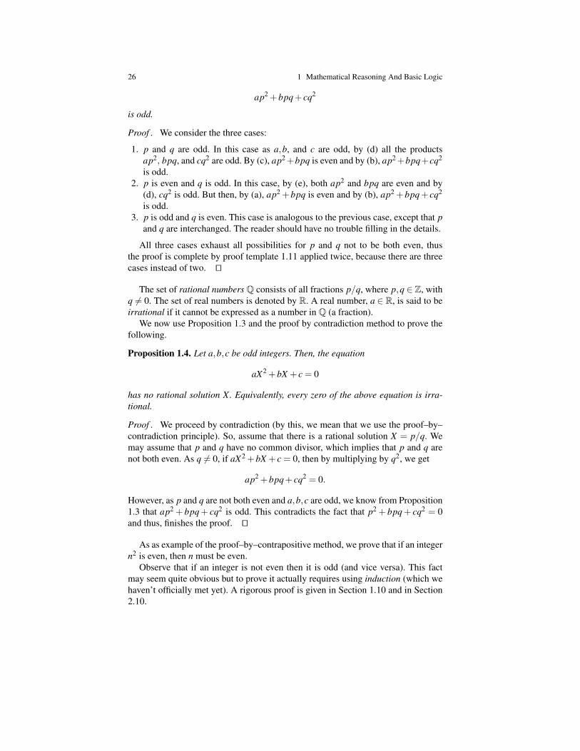
26 1 Mathematical Reasoning And Basic Logic
ap2 +bpq+ cq2
is odd.
Proof . We consider the three cases:
1. p and q are odd. In this case as a,b, and c are odd, by (d) all the productsap2, bpq, and cq2 are odd. By (c), ap2+bpq is even and by (b), ap2+bpq+cq2
is odd.2. p is even and q is odd. In this case, by (e), both ap2 and bpq are even and by
(d), cq2 is odd. But then, by (a), ap2 +bpq is even and by (b), ap2 +bpq+ cq2
is odd.3. p is odd and q is even. This case is analogous to the previous case, except that p
and q are interchanged. The reader should have no trouble filling in the details.
All three cases exhaust all possibilities for p and q not to be both even, thusthe proof is complete by proof template 1.11 applied twice, because there are threecases instead of two. ut
The set of rational numbers Q consists of all fractions p/q, where p,q ∈ Z, withq 6= 0. The set of real numbers is denoted by R. A real number, a ∈ R, is said to beirrational if it cannot be expressed as a number in Q (a fraction).
We now use Proposition 1.3 and the proof by contradiction method to prove thefollowing.
Proposition 1.4. Let a,b,c be odd integers. Then, the equation
aX2 +bX + c = 0
has no rational solution X. Equivalently, every zero of the above equation is irra-tional.
Proof . We proceed by contradiction (by this, we mean that we use the proof–by–contradiction principle). So, assume that there is a rational solution X = p/q. Wemay assume that p and q have no common divisor, which implies that p and q arenot both even. As q 6= 0, if aX2 +bX + c = 0, then by multiplying by q2, we get
ap2 +bpq+ cq2 = 0.
However, as p and q are not both even and a,b,c are odd, we know from Proposition1.3 that ap2 + bpq+ cq2 is odd. This contradicts the fact that p2 + bpq+ cq2 = 0and thus, finishes the proof. ut
As as example of the proof–by–contrapositive method, we prove that if an integern2 is even, then n must be even.
Observe that if an integer is not even then it is odd (and vice versa). This factmay seem quite obvious but to prove it actually requires using induction (which wehaven’t officially met yet). A rigorous proof is given in Section 1.10 and in Section2.10.

1.6 Formal Versus Informal Proofs; Some Examples 27
Now, the contrapositive of our statement is: if n is odd, then n2 is odd. But, tosay that n is odd is to say that n = 2k+1 and then, n2 = (2k+1)2 = 4k2 +4k+1 =2(2k2 +2k)+1, which shows that n2 is odd.
As another illustration of the proof methods that we have just presented, let usprove that
√2 is irrational, which means that
√2 is not rational. The reader may also
want to look at the proof given by Gowers in Chapter 3 of his book [10]. Obviously,our proof is similar but we emphasize step (2) a little more.
Because we are trying to prove that√
2 is not rational, we use Proof Template1.4. Thus, let us assume that
√2 is rational and derive a contradiction. Here are the
steps of the proof.
1. If√
2 is rational, then there exist some integers p,q ∈ Z, with q 6= 0, so that√2 = p/q.
2. Any fraction p/q is equal to some fraction r/s, where r and s are not both even.3. By (2), we may assume that √
2 =pq,
where p,q ∈ Z are not both even and with q 6= 0.4. By (3), because q 6= 0, by multiplying both sides by q, we get
q√
2 = p.
5. By (4), by squaring both sides, we get
2q2 = p2.
6. Inasmuch as p2 = 2q2, the number p2 must be even. By a fact previously estab-lished, p itself is even; that is, p = 2s, for some s ∈ Z.
7. By (6), if we substitute 2s for p in the equation in (5) we get 2q2 = 4s2. Bydividing both sides by 2, we get
q2 = 2s2.
8. By (7), we see that q2 is even, from which we deduce (as above) that q itself iseven.
9. Now, assuming that√
2 = p/q where p and q are not both even (and q 6= 0),we concluded that both p and q are even (as shown in (6) and(8)), reachinga contradiction. Therefore, by negation introduction, we proved that
√2 is not
rational.
A closer examination of the steps of the above proof reveals that the only stepthat may require further justification is step (2): that any fraction p/q is equal tosome fraction r/s where r and s are not both even.
This fact does require a proof and the proof uses the division algorithm, whichitself requires induction (see Section 7.3, Theorem 7.7). Besides this point, all theother steps only require simple arithmetic properties of the integers and are con-structive.
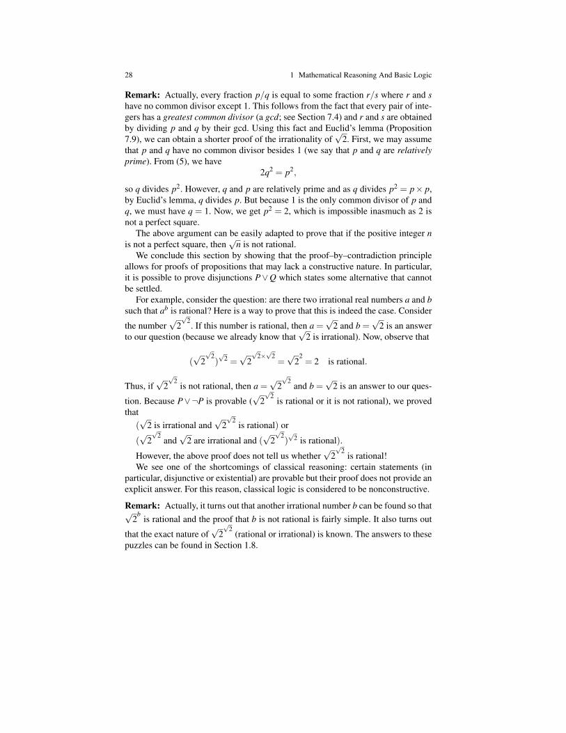
28 1 Mathematical Reasoning And Basic Logic
Remark: Actually, every fraction p/q is equal to some fraction r/s where r and shave no common divisor except 1. This follows from the fact that every pair of inte-gers has a greatest common divisor (a gcd; see Section 7.4) and r and s are obtainedby dividing p and q by their gcd. Using this fact and Euclid’s lemma (Proposition7.9), we can obtain a shorter proof of the irrationality of
√2. First, we may assume
that p and q have no common divisor besides 1 (we say that p and q are relativelyprime). From (5), we have
2q2 = p2,
so q divides p2. However, q and p are relatively prime and as q divides p2 = p× p,by Euclid’s lemma, q divides p. But because 1 is the only common divisor of p andq, we must have q = 1. Now, we get p2 = 2, which is impossible inasmuch as 2 isnot a perfect square.
The above argument can be easily adapted to prove that if the positive integer nis not a perfect square, then
√n is not rational.
We conclude this section by showing that the proof–by–contradiction principleallows for proofs of propositions that may lack a constructive nature. In particular,it is possible to prove disjunctions P∨Q which states some alternative that cannotbe settled.
For example, consider the question: are there two irrational real numbers a and bsuch that ab is rational? Here is a way to prove that this is indeed the case. Consider
the number√
2√
2. If this number is rational, then a =
√2 and b =
√2 is an answer
to our question (because we already know that√
2 is irrational). Now, observe that
(√
2√
2)√
2 =√
2√
2×√
2=√
22= 2 is rational.
Thus, if√
2√
2is not rational, then a =
√2√
2and b =
√2 is an answer to our ques-
tion. Because P∨¬P is provable (√
2√
2is rational or it is not rational), we proved
that(√
2 is irrational and√
2√
2is rational) or
(√
2√
2and√
2 are irrational and (√
2√
2)√
2 is rational).
However, the above proof does not tell us whether√
2√
2is rational!
We see one of the shortcomings of classical reasoning: certain statements (inparticular, disjunctive or existential) are provable but their proof does not provide anexplicit answer. For this reason, classical logic is considered to be nonconstructive.
Remark: Actually, it turns out that another irrational number b can be found so that√2
bis rational and the proof that b is not rational is fairly simple. It also turns out
that the exact nature of√
2√
2(rational or irrational) is known. The answers to these
puzzles can be found in Section 1.8.

1.7 Truth Tables and Truth Value Semantics 29
1.7 Truth Tables and Truth Value Semantics
So far, we have deliberately focused on the construction of proofs using proof tem-plates, we but have ignored the notion of truth. We can’t postpone any longer adiscussion of the truth value semantics for classical propositional logic.
We all learned early on that the logical connectives ⇒, ∧, ∨, ¬ and ≡ can beinterpreted as Boolean functions, that is, functions whose arguments and whosevalues range over the set of truth values,
BOOL = true, false.
These functions are given by the following truth tables.
P Q P⇒ Q P∧Q P∨Q ¬P P≡ Qtrue true true true true false truetrue false false false true false falsefalse true true false true true falsefalse false true false false true true
Note that the implication P⇒ Q is false (has the value false) exactly when P =false and Q = true.
Now, any proposition P built up over the set of atomic propositions PS (ourpropositional symbols) contains a finite set of propositional letters, say
P1, . . . ,Pm.
If we assign some truth value (from BOOL) to each symbol Pi then we can “com-pute” the truth value of P under this assignment by using recursively using the truthtables above. For example, the proposition P1⇒ (P1⇒ P2), under the truth assign-ment v given by
P1 = true, P2 = false,
evaluates to false. Indeed, the truth value, v(P1⇒ (P1⇒ P2)), is computed recur-sively as
v(P1⇒ (P1⇒ P2)) = v(P1)⇒ v(P1⇒ P2).
Now, v(P1) = true and v(P1⇒ P2) is computed recursively as
v(P1⇒ P2) = v(P1)⇒ v(P2).
Because v(P1) = true and v(P2) = false, using our truth table, we get
v(P1⇒ P2) = true⇒ false = false.
Plugging this into the right-hand side of v(P1⇒ (P1⇒ P2)), we finally get
v(P1⇒ (P1⇒ P2)) = true⇒ false = false.
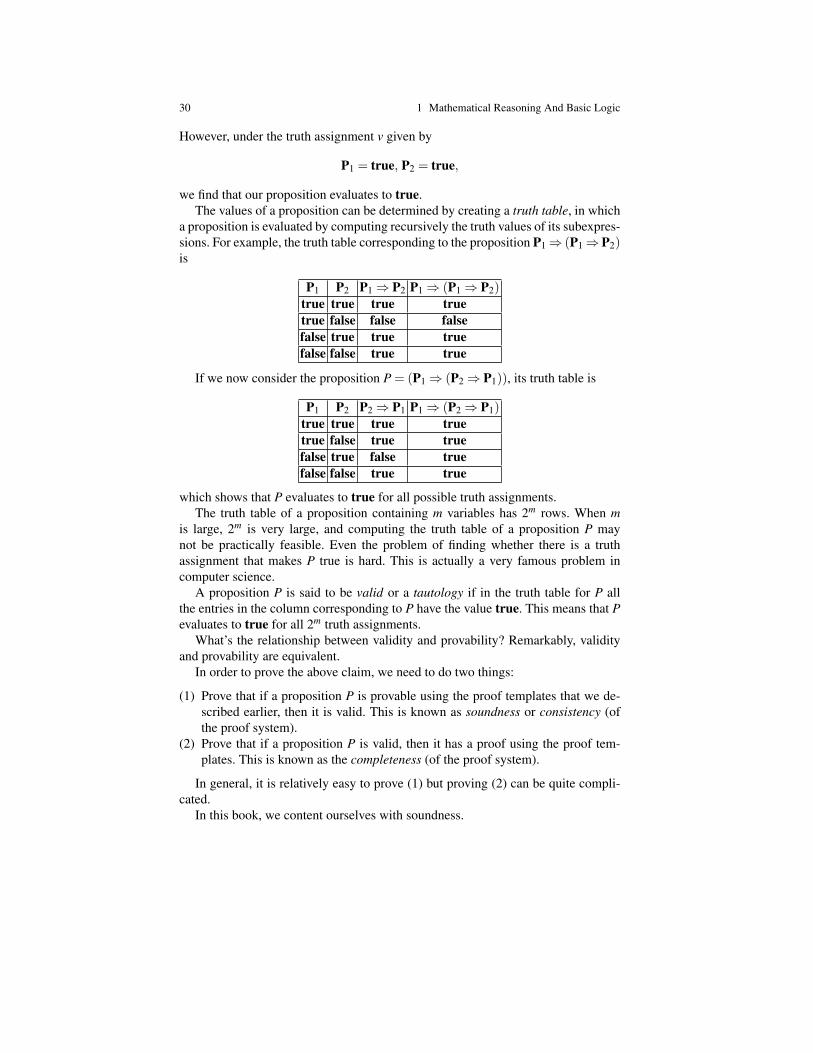
30 1 Mathematical Reasoning And Basic Logic
However, under the truth assignment v given by
P1 = true, P2 = true,
we find that our proposition evaluates to true.The values of a proposition can be determined by creating a truth table, in which
a proposition is evaluated by computing recursively the truth values of its subexpres-sions. For example, the truth table corresponding to the proposition P1⇒ (P1⇒P2)is
P1 P2 P1⇒ P2 P1⇒ (P1⇒ P2)
true true true truetrue false false falsefalse true true truefalse false true true
If we now consider the proposition P = (P1⇒ (P2⇒ P1)), its truth table is
P1 P2 P2⇒ P1 P1⇒ (P2⇒ P1)
true true true truetrue false true truefalse true false truefalse false true true
which shows that P evaluates to true for all possible truth assignments.The truth table of a proposition containing m variables has 2m rows. When m
is large, 2m is very large, and computing the truth table of a proposition P maynot be practically feasible. Even the problem of finding whether there is a truthassignment that makes P true is hard. This is actually a very famous problem incomputer science.
A proposition P is said to be valid or a tautology if in the truth table for P allthe entries in the column corresponding to P have the value true. This means that Pevaluates to true for all 2m truth assignments.
What’s the relationship between validity and provability? Remarkably, validityand provability are equivalent.
In order to prove the above claim, we need to do two things:
(1) Prove that if a proposition P is provable using the proof templates that we de-scribed earlier, then it is valid. This is known as soundness or consistency (ofthe proof system).
(2) Prove that if a proposition P is valid, then it has a proof using the proof tem-plates. This is known as the completeness (of the proof system).
In general, it is relatively easy to prove (1) but proving (2) can be quite compli-cated.
In this book, we content ourselves with soundness.
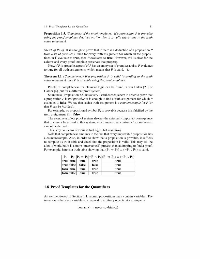
1.8 Proof Templates for the Quantifiers 31
Proposition 1.5. (Soundness of the proof templates) If a proposition P is provableusing the proof templates desribed earlier, then it is valid (according to the truthvalue semantics).
Sketch of Proof . It is enough to prove that if there is a deduction of a proposition Pfrom a set of premises Γ then for every truth assignment for which all the proposi-tions in Γ evaluate to true, then P evaluates to true. However, this is clear for theaxioms and every proof template preserves that property.
Now, if P is provable, a proof of P has an empty set of premises and so P evaluatesto true for all truth assignments, which means that P is valid. ut
Theorem 1.1. (Completeness) If a proposition P is valid (according to the truthvalue semantics), then P is provable using the proof templates.
Proofs of completeness for classical logic can be found in van Dalen [23] orGallier [4] (but for a different proof system).
Soundness (Proposition 2.8) has a very useful consequence: in order to prove thata proposition P is not provable, it is enough to find a truth assignment for which Pevaluates to false. We say that such a truth assignment is a counterexample for P (orthat P can be falsified).
For example, no propositional symbol Pi is provable because it is falsified by thetruth assignment Pi = false.
The soundness of our proof system also has the extremely important consequencethat ⊥ cannot be proved in this system, which means that contradictory statementscannot be derived.
This is by no means obvious at first sight, but reassuring.Note that completeness amounts to the fact that every unprovable proposition has
a counterexample. Also, in order to show that a proposition is provable, it sufficesto compute its truth table and check that the proposition is valid. This may still bea lot of work, but it is a more “mechanical” process than attempting to find a proof.For example, here is a truth table showing that (P1⇒ P2)≡ (¬P1∨P2) is valid.
P1 P2 P1⇒ P2 ¬P1∨P2 (P1⇒ P2)≡ (¬P1∨P2)
true true true true truetrue false false false truefalse true true true truefalse false true true true
1.8 Proof Templates for the Quantifiers
As we mentioned in Section 1.1, atomic propositions may contain variables. Theintention is that such variables correspond to arbitrary objects. An example is
human(x)⇒ needs-to-drink(x).
32 1 Mathematical Reasoning And Basic Logic
Now, in mathematics, we usually prove universal statements, that is statements thathold for all possible “objects,” or existential statements, that is, statements assertingthe existence of some object satisfying a given property. As we saw earlier, we assertthat every human needs to drink by writing the proposition
∀x(human(x)⇒ needs-to-drink(x)).
The symbol ∀ is called a universal quantifier. Observe that once the quantifier ∀(pronounced “for all” or “for every”) is applied to the variable x, the variable xbecomes a placeholder and replacing x by y or any other variable does not changeanything. We say that x is a bound variable (sometimes a “dummy variable”).
If we want to assert that some human needs to drink we write
∃x(human(x)⇒ needs-to-drink(x));
The symbol ∃ is called an existential quantifier. Again, once the quantifier ∃ (pro-nounced “there exists”) is applied to the variable x, the variable x becomes a place-holder. However, the intended meaning of the second proposition is very differentand weaker than the first. It only asserts the existence of some object satisfying thestatement
human(x)⇒ needs-to-drink(x).
Statements may contain variables that are not bound by quantifiers. For example,in
∃x parent(x,y)
the variable x is bound but the variable y is not. Here, the intended meaning ofparent(x,y) is that x is a parent of y, and the intended meaning of ∃x parent(x,y) isthat any given y has some parent x. Variables that are not bound are called free. Theproposition
∀y∃x parent(x,y),
which contains only bound variables is meant to assert that every y has some par-ent x. Typically, in mathematics, we only prove statements without free variables.However, statements with free variables may occur during intermediate stages of aproof.
Now, in addition to propositions of the form P∧Q,P∨Q,P⇒ Q,¬P,P≡ Q, weadd two new kinds of propositions (also called formulae):
1. Universal formulae, which are formulae of the form ∀xP, where P is any for-mula and x is any variable.
2. Existential formulae, which are formulae of the form ∃xP, where P is any for-mula and x is any variable.
The intuitive meaning of the statement ∀xP is that P holds for all possible objectsx and the intuitive meaning of the statement ∃xP is that P holds for some object x.Thus, we see that it would be useful to use symbols to denote various objects. Forexample, if we want to assert some facts about the “parent” predicate, we may want

1.8 Proof Templates for the Quantifiers 33
to introduce some constant symbols (for short, constants) such as “Jean,” “Mia,” andso on and write
parent(Jean,Mia)
to assert that Jean is a parent of Mia. Often, we also have to use function symbols(or operators, constructors), for instance, to write a statement about numbers: +, ∗,and so on. Using constant symbols, function symbols, and variables, we can formterms, such as
(x∗ x+1)∗ (3∗ y+2).
In addition to function symbols, we also use predicate symbols, which are namesfor atomic properties. We have already seen several examples of predicate symbols:“odd,” “even,” “prime,” “human,” “parent.” So, in general, when we try to proveproperties of certain classes of objects (people, numbers, strings, graphs, and soon), we assume that we have a certain alphabet consisting of constant symbols,function symbols, and predicate symbols. Using these symbols and an infinite sup-ply of variables we can form terms and predicate terms. We say that we have a(logical) language. Using this language, we can write compound statements. A de-tailed presentation of this approach is given in Chapter 2. Here, we follow a moreinformal and more intuitive approach. We use the notion of term as a synonym forsome specific object. Terms are often denoted by the Greek letter τ , sometimes sub-scripted. A variable qualifies as a term.
When working with propositions possibly containing quantifiers, it is customaryto use the term formula instead of proposition. The term proposition is typicallyreserved to formulae wihout quantifiers.
Unlike the Proof Templates for⇒,∨,∧ and ⊥, which are rather straightforward,the Proof Templates for quantifiers are more subtle due to the presence of variables(occurring in terms and predicates) and the fact that it is sometimes necessary tomake substitutions.
Given a formula P containing some free variable x and given a term τ , the resultof replacing all occurrences of x by τ in P is called a substitution and is denotedP[τ/x] (and pronounced “the result of substituting τ for x in P”). Substitutions canbe defined rigorously by recursion. Let us simply give an example Consider thepredicate P(x) = odd(2x+ 1). If we substitute the term τ = (y+ 1)2 for x in P(x),we obtain
P[τ/x] = odd(2(y+1)2 +1).
We have to be careful to forbid inferences that would yield “wrong” results whenwe perform substitutions, and for this we have to be very precise about the way weuse free variables. Again, these issues are delt with in Chapter 2. In this chapter, wewill content ourselves with some warnings.
We begin with the proof templates for the universal quantifier.
Proof Template 1.14. (Forall–Intro)
Let Γ be a list of premises and let y be a variable that does not occur free in anypremise in Γ or in ∀xP. If we have a deduction of the formula P[y/x] from Γ , thenwe obtain a deduction of ∀xP from Γ .
34 1 Mathematical Reasoning And Basic Logic
Proof Template 1.15. (Forall–Elim)
Let Γ be a list of premises and let τ be a term representing some specific object. Ifwe have a deduction of ∀xP from Γ , then we obtain a deduction of P[τ/x] from Γ .
The Proof Template 1.14 may look a little strange but the idea behind it is actuallyvery simple: Because y is totally unconstrained, if P[y/x] (the result of replacing alloccurrences of x by y in P) is provable (from Γ ), then intuitively P[y/x] holds forany arbitrary object, and so, the statement ∀xP should also be provable (from Γ ).
Note that we can’t deduce ∀xP from P[y/x] because the deduction has the singlepremise P[y/x] and y occurs in P[y/x] (unless x does not occur in P).
The meaning of the Proof Template 1.15 is that if ∀xP is provable (from Γ ), thenP holds for all objects and so, in particular for the object denoted by the term τ; thatis, P[τ/x] should be provable (from Γ ).
Here are the proof templates for the existential quantifier.
Proof Template 1.16. (Exist–Intro)
Let Γ be a list of premises and let τ be a term representing some specific object. Ifwe have a deduction of P[τ/x] from Γ , then we obtain a deduction of ∃xP(x) fromΓ .
Proof Template 1.17. (Exist–Elim)
Let Γ be a list of premises. Let C and ∃xP be formulae, and let y be a variable thatdoes not occur free in any premise in Γ , in ∃xP, or in C. To obtain a deduction of Cfrom Γ , proceed as follows:
1. Make a deduction of ∃xP from Γ .2. Add P[y/x] as a premise to Γ , and find a deduction of C from P[y/x] and Γ .3. Delete the premise P[y/x].
If P[τ/x] is provable (from Γ ), this means that the object denoted by τ satisfies P,so ∃xP should be provable (this latter formula asserts the existence of some objectsatisfying P, and τ is such an object).
Proof Template 1.17 is reminiscent of the proof–by–cases principle (Proof tem-plate 1.11) and is a little more tricky. It goes as follows. Suppose that we proved∃xP (from Γ ). Moreover, suppose that for every possible case P[y/x] we were ableto prove C (from Γ ). Then, as we have “exhausted” all possible cases and as weknow from the provability of ∃xP that some case must hold, we can conclude that Cis provable (from Γ ) without using P[y/x] as a premise.
Like the the proof–by–cases principle, Proof Template 1.17 is not very construc-tive. It allows making a conclusion (C) by considering alternatives without knowingwhich one actually occurs.
Constructing proofs using the proof templates for the quantifiers can be quitetricky due to the restrictions on variables. In practice, we always use “fresh” (brandnew) variables to avoid problems. Also, when we use Proof Template 1.14, we beginby saying “let y be arbitrary,” then we prove P[y/x] (mentally substituting y for x),
1.8 Proof Templates for the Quantifiers 35
and we conclude with: “since y is arbitrary, this proves ∀xP.” We proceed in a similarway when using Proof Template 1.17, but this time we say “let y be arbitrary” in step(2). When we use Proof Template 1.15, we usually say: “Since ∀xP holds, it holdsfor all x, so in particular it holds for τ , and thus P[τ/x] holds.” Similarly, whenusing Proof Template 1.16, we say “since P[τ/x] holds for a specific object τ , wecan deduce that ∃xP holds.”
Let us give two examples of a proof using the proof templates for ∀ and ∃.Example 1.21. For any natural number n, let odd(n) be the predicate that asserts thatn is odd, namely
odd(n)≡ ∃m((m ∈ N)∧ (n = 2m+1)).
First, let us prove that∀a((a ∈ N)⇒ odd(2a+1)).
By Proof Template 1.14, let x be a fresh variable; we need to prove
(x ∈ N)⇒ odd(2x+1).
By Proof Template 1.2, assume x ∈ N. If we consider the formula
(m ∈ N)∧ (2x+1 = 2m+1),
by substituting x for m, we get
(x ∈ N)∧ (2x+1 = 2x+1),
which is provable since x ∈ N. By Proof Template 1.16, we obtain
∃m(m ∈ N)∧ (x = 2m+1);
that is, odd(x) is provable. Using Proof Template 1.2, we delete the premise x ∈ Nand we have proved
(x ∈ N)⇒ odd(2x+1).
This proof has no longer any premises, so we can safely conclude that
∀a((a ∈ N)⇒ odd(2a+1)).
Next, consider the term τ = 7. By Proof Template 1.15, we obtain
(7 ∈ N)⇒ odd(15).
Since 7 ∈ N, by modus ponens we deduce that 15 is odd.Let us now consider the term τ = (b+1)2 with b ∈ N. By Proof Template 1.15,
we obtain((b+1)2 ∈ N)⇒ odd(2(b+1)2 +1)).
But b ∈ N implies that (b+ 1)2 ∈ N so by modus ponens and Proof Template 1.2,we deduce that
36 1 Mathematical Reasoning And Basic Logic
(b ∈ N)⇒ odd(2(b+1)2 +1)).
Example 1.22. Let us prove the formula ∀x(P∧Q)⇒∀xP∧∀xQ.First, using Proof Template 1.2, we assume ∀x(P∧Q) (two copies). The next step
uses a trick. Since variables are terms, if u is a fresh variable, then by Proof Templare1.15 we deduce (P∧Q)[u/x]. Now we use a property of substitutions which saysthat
(P∧Q)[u/x] = P[u/x]∧Q[u/x].
We can now use Proof Template 1.9 (twice) to deduce P[u/x] and Q[u/x]. But, re-member that the premise is ∀x(P∧Q) (two copies), and since u is a fresh variable,it does not occur in this premise, so we can safely apply Proof Template 1.14 andconclude ∀xP, and similarly ∀xQ. By Proof Template 1.8, we deduce ∀xP∧∀xQfrom ∀x(P∧Q). Finally, by Proof Template 1.2, we delete the premise ∀x(P∧Q)and obtain our proof. The above proof has the following tree representation.
∀x(P∧Q)x√
P[u/x]∧Q[u/x]
P[u/x]
∀xP
∀x(P∧Q)x√
P[u/x]∧Q[u/x]
Q[u/x]
∀xQ
∀xP∧∀xQx
∀x(P∧Q)⇒∀xP∧∀xQ
The reader should show that ∀xP∧∀xQ⇒∀x(P∧Q) is also provable.However, in general, one can’t just replace ∀ by ∃ (or ∧ by ∨) and still obtain
provable statements. For example, ∃xP∧∃xQ⇒∃x(P∧Q) is not provable at all.Here are some useful equivalences involving quantifiers. The first two are analo-
gous to the de Morgan laws for ∧ and ∨.
Proposition 1.6. The following formulae are provable:
¬∀xP≡ ∃x¬P
¬∃xP≡ ∀x¬P
∀x(P∧Q)≡ ∀xP∧∀xQ
∃x(P∨Q)≡ ∃xP∨∃xQ
∃x(P∧Q)⇒∃xP∧∃xQ
∀xP∨∀xQ⇒∀x(P∨Q).
The proof system that uses all the Proof Templates that we have defined provesformulae of classical first-order logic.
One should also be careful that the order the quantifiers is important. For exam-ple, a formula of the form
∀x∃yP
1.9 Sets and Set Operations 37
is generally not equivalent to the formula
∃y∀xP.
The second formula asserts the existence of some object y such that P holds for allx. But in the first formula, for every x, there is some y such that P holds, but each ydepends on x and there may not be a single y that works for all x.
Another amusing mistake involves negating a universal quantifier. The formula∀x¬P is not equivalent to ¬∀xP. Once traveling from Philadelphia to New York Iheard a train conductor say: “all doors will not open.” Actually, he meant “not alldoors will open,” which would give us a chance to get out!
Remark: We can illustrate, again, the fact that classical logic allows for noncon-structive proofs by re-examining the example at the end of Section 1.4. There, we
proved that if√
2√
2is rational, then a =
√2 and b =
√2 are both irrational numbers
such that ab is rational and if√
2√
2is irrational then a =
√2√
2and b =
√2 are both
irrational numbers such that ab is rational. By Proof Template 1.16, we deduce that
if√
2√
2is rational then there exist some irrational numbers a,b so that ab is rational
and if√
2√
2is irrational then there exist some irrational numbers a,b so that ab is
rational. In classical logic, as P∨¬P is provable, by the proof–by–cases principlewe just proved that there exist some irrational numbers a and b so that ab is rational.
However, this argument does not give us explicitly numbers a and b with therequired properties. It only tells us that such numbers must exist.
Now, it turns out that√
2√
2is indeed irrational (this follows from the Gel’fond–
Schneider theorem, a hard theorem in number theory). Furthermore, there are alsosimpler explicit solutions such as a =
√2 and b = log2 9, as the reader should check.
1.9 Sets and Set Operations
In this section we review the definition of a set and basic set operations. This sec-tion takes the “naive” point of view that a set is an unordered collection of objects,without duplicates, the collection being regarded as a single object.
Given a set A we write that some object a is an element of (belongs to) the set Aas
a ∈ A
and that a is not an element of A (does not belong to A) as
a /∈ A.
The symbol ∈ is the set membership symbol.A set can either be defined explicitely by listing its elements within curly braces
(the symbols and ) or as a collection of objects satisfying a certain property. For
38 1 Mathematical Reasoning And Basic Logic
example, the set C consisting of the colors red, blue, green is given by
C = red,blue,green.
Because the order of elements in a set is irrelevant, the set C is also given by
C = green, red,blue.
In fact, a moment of reflexion reveals that there are six ways of writing the set C.If we denote by N the set of natural numbers
N= 0,1,2,3, . . .,
then the set E of even integers can be defined in terms of the property even of beingeven by
E = n ∈ N | even(n).More generally, given some property P and some set X , we denote the set of allelements of X that satisfy the property P by
x ∈ X | P(x) or x | x ∈ X ∧P(x).
When are two sets A and B equal? The answer is given by the first proof templateof set theory, called the Extensionality Axiom.
Proof Template 1.18. (Extensionality Axiom)
Two sets A and B are equal iff they have exactly the same elements; that is, everyelement of A is an element of B and conversely. This can be written more formallyas
∀x(x ∈ A⇒ x ∈ B)∧∀x(x ∈ B⇒ x ∈ A).
There is a special set having no elements at all, the empty set, denoted /0. Theempty set is characterized by the property
∀x(x /∈ /0).
Next, we define the notion of inclusion between sets
Definition 1.5. Given any two sets, A and B, we say that A is a subset of B (or thatA is included in B), denoted A ⊆ B, iff every element of A is also an element of B,that is,
∀x(x ∈ A⇒ x ∈ B).
We say that A is a proper subset of B iff A ⊆ B and A 6= B. This implies that thatthere is some b ∈ B with b /∈ A. We usually write A⊂ B.
For example, if A = green,blue and C = green, red,blue, then
A⊆C.
1.9 Sets and Set Operations 39
Note that the empty set is a subset of every set.Observe the important fact that equality of two sets can be expressed by
A = B iff A⊆ B and B⊆ A.
Proving that two sets are equal may be quite complicated if the definitions ofthese sets are complex, and the above method is the safe one.
If a set A has a finite number of elements, then this number (a natural number)is called the cardinality of the set and is denoted by |A| (sometimes by card(A)).Otherwise, the set is said to be infinite. The cardinality of the empty set is 0.
Sets can be combined in various ways, just as numbers can be added, multiplied,etc. However, operations on sets tend to minic logical operations such as disjunction,conjunction, and negation, rather than the arithmetical operations on numbers. Themost basic operations are union, intersection, and relative complement.
Definition 1.6. For any two sets A and B, the union of A and B is the set A∪ Bdefined such that
x ∈ A∪B iff (x ∈ A)∨ (x ∈ B).
This reads, x is a member of A∪B if either x belongs to A or x belongs to B (orboth). We also write
A∪B = x | x ∈ A or x ∈ B.The intersection of A and B is the set A∩B defined such that
x ∈ A∩B iff (x ∈ A)∧ (x ∈ B).
This reads, x is a member of A∩B if x belongs to A and x belongs to B. We alsowrite
A∩B = x | x ∈ A and x ∈ B.The relative complement (or set difference) of A and B is the set A−B defined suchthat
x ∈ A−B iff (x ∈ A)∧¬(x ∈ B).
This reads, x is a member of A−B if x belongs to A and x does not belong to B. Wealso write
A−B = x | x ∈ A and x /∈ B.For example, if A = 0,2,4,6 and B = 0,1,3,5, then
A∪B = 0,1,2,3,4,5,6A∩B = 0A−B = 2,4,6.
Two sets A,B are said to be disjoint if A∩B = /0. It is easy to see that if A and Bare two finite sets and if A and B are disjoint, then
|A∪B|= |A|+ |B|.

40 1 Mathematical Reasoning And Basic Logic
In general, by writing
A∪B = (A∩B)∪ (A−B)∪ (B−A),
if A and B are finite, it can be shown that
|A∪B|= |A|+ |B|− |A∩B|.
The situation in which we maniplulate subsets of some fixed set X often arises,and it is useful to introduce a special type of relative complement with respect to X .For any subset A of X , the complement A of A in X is defined by
A = X−A,
which can also be expressed as
A = x ∈ X | x /∈ A.
Using the union operation, we can form bigger sets by taking unions with single-tons. For example, we can form
a,b,c= a,b∪c.
Remark: We can systematically construct bigger and bigger sets by the followingmethod: Given any set A let
A+ = A∪A.If we start from the empty set, we obtain the sets
/0, /0, /0, /0, /0, /0, /0, /0, etc.
These sets can be used to define the natural numbers and the + operation corre-sponds to the successor function on the natural numbers (i.e., n 7→ n+1).
The algebraic properties of union, intersection, and complementation are inher-ited from the properties of disjunction, conjunction, and negation. The followingproposition lists some of the most important properties of union, intersection, andcomplementation.
Proposition 1.7. The following equations hold for all sets A,B,C:
A∪ /0 = A
A∩ /0 = /0A∪A = A
A∩A = A
A∪B = B∪A
A∩B = B∩A.

1.9 Sets and Set Operations 41
The last two assert the commutativity of ∪ and ∩. We have distributivity of ∩ over ∪and of ∪ over ∩:
A∩ (B∪C) = (A∩B)∪ (A∩C)
A∪ (B∩C) = (A∪B)∩ (A∪C).
We have associativity of ∩ and ∪:
A∩ (B∩C) = (A∩B)∩C
A∪ (B∪C) = (A∪B)∪C.
Proof . We use Proposition 1.2. Let us prove that A∩ (B∪C) = (A∩B)∪ (A∩C),leaving the proof of the other equations as an exercise. We prove the two inclusionsA∩ (B∪C)⊆ (A∩B)∪ (A∩C) and (A∩B)∪ (A∩C)⊆ A∩ (B∪C).
Assume that x ∈ A∩ (B∪C). This means that x ∈ A and x ∈ B∪C; that is,
(x ∈ A)∧ ((x ∈ B)∨ (x ∈C)).
Using the distributivity of ∧ over ∨, we obtain
((x ∈ A)∧ (x ∈ B))∨ ((x ∈ A)∧ (x ∈C)).
But, the above says that x ∈ (A∩B)∪ (A∩C), which proves our first inclusion.Conversely assume that x ∈ (A∩B)∪ (A∩C). This means that x ∈ (A∩B) or
x ∈ (A∩C); that is,
((x ∈ A)∧ (x ∈ B))∨ ((x ∈ A)∧ (x ∈C)).
Using the distributivity of ∧ over ∨ (in the other direction), we obtain
(x ∈ A)∧ ((x ∈ B)∨ (x ∈C)),
which says that x ∈ A∩ (B∪C), and proves our second inclusion.Note that we could have avoided two arguments by proving that x ∈ A∩ (B∪C)
iff (A∩B)∪ (A∩C) using the fact that the distributivity of ∧ over ∨ is a logicalequivalence. ut
We also have the following version of Proposition 1.2 for subsets.
Proposition 1.8. For every set X and any two subsets A,B of X, the following iden-tities hold:
A = A
(A∩B) = A∪B
(A∪B) = A∩B.
The last two are de Morgan laws.

42 1 Mathematical Reasoning And Basic Logic
Another operation is the power set formation. It is indeed a “powerful” operation,in the sense that it allows us to form very big sets.
Definition 1.7. Given any set A, there is a set P(A) also denoted 2A called thepower set of A whose members are exactly the subsets of A; that is,
X ∈P(A) iff X ⊆ A.
For example, if A = a,b,c, then
P(A) = /0,a,b,c,a,b,a,c,b,c,a,b,c,
a set containing eight elements. Note that the empty set and A itself are alwaysmembers of P(A).
Remark: If A has n elements, it is not hard to show that P(A) has 2n elements.For this reason, many people, including me, prefer the notation 2A for the power setof A.
It is possible to define the union of possibly infinitely many sets. Given any setX (think of X as a set of sets), there is a set
⋃X defined so that
x ∈⋃
X iff ∃B(B ∈ X ∧ x ∈ B).
This says that⋃
X consists of all elements that belong to some member of X .If we take X = A,B, where A and B are two sets, we see that⋃
A,B= A∪B.
Observe that ⋃A= A,
⋃A1, . . . ,An= A1∪·· ·∪An.
and in particular,⋃
/0 = /0.We can also define infinite intersections. For every nonempty set X there is a set⋂
X defined byx ∈
⋂X iff ∀B(B ∈ X ⇒ x ∈ B).
Observe that⋂A,B= A∩B,
⋂A1, . . . ,An= A1∩·· ·∩An.
However,⋂
/0 is undefined. Indeed,⋂
/0 would have to be the set of all sets, since thecondition
∀B(B ∈ /0⇒ x ∈ B)
holds trivially for all B (as the empty set has no members). However there is no suchset, because its existence would lead to a paradox! This point is discussed is Chapter2. Let us simply say that dealing with big infinite sets is tricky.

1.10 Induction and the Well–Ordering Principle on the Natutal Numbers 43
Thorough and yet accessible presentations of set theory can be found in Halmos[5] and Enderton [1].
We close this chapter with a quick discussion of the natural numbers.
1.10 Induction and the Well–Ordering Principle on the NatutalNumbers
Recall that the set of natural numbers is the set N given by
N= 0,1,2,3, . . ..
In this chapter, we do not attempt to define the natural numbers from other concepts,such as sets. We assume that they are “God given.” One of our main goals is to proveproperties of the natural numbers. For this, certain subsets called inductive play acrucial role.
Definition 1.8. We say that a subset S of N is inductive iff
(1) 0 ∈ S.(2) For every n ∈ S, we have n+1 ∈ S.
One of the most important proof principles for the natural numbers is the follow-ing:
Proof Template 1.19. (Induction Principle for N)Every inductive subset S of N is equal to N itself; that is S = N.
Let us give one example illustrating Proof Template 1.19. Many more examplesare given in Chapter 3.
Example 1.23. We prove that for every real number a 6= 1 and evey natural numbern, we have
1+a+ · · ·+an =an+1−1
a−1.
This can also be written asn
∑i=1
ai =an+1−1
a−1, (∗)
with the convention that a0 = 1, even if a = 0. Let S be the set of natural numbers nfor which the identity (∗) holds, and let us prove that S is inductive.
First, we need to prove that 0 ∈ S. The lefthand side becomes a0 = 1, and therighthand side is (a− 1)/(a− 1), which is equal to 1 since we assume that a 6= 1.Therefore, (∗) holds for n = 0; that is, 0 ∈ S.
Next, assume that n∈ S (this is called the induction hypothesis). We need to provethat n+1 ∈ S. Observe that

44 1 Mathematical Reasoning And Basic Logic
n+1
∑i=1
ai =n
∑i=1
ai +an+1.
Now, since we assumed that n ∈ S, we have
n
∑i=1
ai =an+1−1
a−1,
and we deduce that
n+1
∑i=1
ai =n
∑i=1
ai +an+1
=an+1−1
a−1+an+1
=an+1−1+an+2−an+1
a−1
=an+2−1
a−1.
This proves that n+1 ∈ S. Therefore, S is inductive, and so S = N.
We show how to rephrase this induction principle a little more conveniently usingthe notion of function in Chapter 3.
Another important property of N is the so-called well–ordering principle. Thisprinciple turns out to be equivalent to the induction principle for N. Such mattersare discussed in Section 7.3. In this chapter, we accept the well–ordering principlewithout proof.
Proof Template 1.20. (Well–Ordering Principle for N)Every nonempty subset of N has a smallest element.
Proof Template 1.20 can be used to prove properties of N by contradiction. Forexample, consider the property that every natural number n is either even or odd.
For the sake of contradiction (here, we use the proof–by–contradiction principle),assume that our statement does not hold. If so, the subset S of natural numbers n forwhich n is neither even nor odd is nonempty. By the well–ordering principle, the setS has a smallest element, say m.
If m = 0, then 0 would be neither even nor odd, a contradiction since 0 is even.Therefore, m > 0. But then, m− 1 /∈ S, since m is the smallest element of S. Thismeans that m− 1 is either even or odd. But if m− 1 is even, then m− 1 = 2k forsome k, so m = 2k+1 is odd, and if m−1 is odd, then m−1 = 2k+1 for some k,so m = 2(k+ 1) is even. We just proved that m is either even or odd, contradictingthe fact that m ∈ S. Therefore, S must be empty and we proved the desired result.
We conclude this section with one more example showing the usefulness of thewell–ordering principle.
1.11 Summary 45
Example 1.24. Suppose we have a property P(n) of the natural numbers such thatP(n) holds for at least some n, and that for every n such that P(n) holds and n≥ 100,then there is some m < n such that P(m) holds. We claim that there is some m < 100such that P(m) holds. Let S be the set of natural numbers n such that P(n) holds.By hypothesis, there is some some n such that P(n) holds, so S is nonempty. Bythe well–ordering principle, the set S has a smallest element, say m. For the sake ofcontradiction, assume that m ≥ 100. Then, since P(m) holds and m ≥ 100, by thehypothesis there is some m′ < m such that P(m′) holds, contradicting the fact that mis the smallest element of S. Therefore, by the proof–by–contradiction principle, weconclude that m < 100, as claimed.
Beware that the well–ordering principle is false for Z, because Z does not have asmallest element.
1.11 Summary
The main goal of this chapter is to describe how to construct proofs in terms ofproof templates. A brief and informal introduction to sets and set operations is alsoprovided.
• We describe the syntax of propositions.• We define the proof templates for implication.• We show that deductions proceed from assumptions (or premises) according to
proof templates.• We introduce falsity ⊥ and negation ¬P as an abbrevation for P⇒⊥. We de-
scribe the proof templates for conjunction, disjunction, and negation.• We show that one of the rules for negation is the proof–by–contradiction rule
(also known as RAA). It plays a special role, in the sense that it allows for theconstruction of indirect proofs.
• We present the proof–by–contrapositive rule.• We present the de Morgan laws as well as some basic properties of ∨ and ∧.• We give some examples of proofs of “real” statements.• We give an example of a nonconstructive proof of the statement: there are two
irrational numbers, a and b, so that ab is rational.• We explain the truth-value semantics of propositional logic.• We define the truth tables for the boolean functions associated with the logical
connectives (and, or, not, implication, equivalence).• We define the notion of validity and tautology.• We discuss soundness (or consistency) and completeness.• We state the soundness and completeness theorems for propositional classical
logic.• We explain how to use counterexamples to prove that certain propositions are
not provable.

46 1 Mathematical Reasoning And Basic Logic
• We add first-order quantifiers (“for all” ∀ and “there exists” ∃) to the languageof propositional logic and define first-order logic.
• We describe free and bound variables.• We describe Proof Templates for the quantifiers.• We prove some “de Morgan”-type rules for the quantified formulae.• We introduce sets and explain when two sets are equal.• We define the notion of subset.• We define some basic operations on sets: the union A∪B, intersection A∩B,
and relative complement A−B.• We define the complement of a subset of a given set.• We prove some basic properties of union, intersection and complementation,
including the de Morgan laws.• We define the power set of a set.• We define inductive subsets of N and state the induction principle for N.• We state the well–ordering principle for N.
Problems
1.1. Give a proof of the proposition (P⇒ Q)⇒ ((P⇒ (Q⇒ R))⇒ (P⇒ R)).
1.2. (a) Prove the “de Morgan” laws:
¬(P∧Q)≡ ¬P∨¬Q
¬(P∨Q)≡ ¬P∧¬Q.
(b) Prove the propositions (P∧¬Q)⇒¬(P⇒ Q) and ¬(P⇒ Q)⇒ (P∧¬Q).
1.3. (a) Prove the equivalences
P∨P≡ P
P∧P≡ P
P∨Q≡ Q∨P
P∧Q≡ Q∧P.
(b) Prove the equivalences
P∧ (P∨Q)≡ P
P∨ (P∧Q)≡ P.
1.4. Prove the propositions
1.11 Problems 47
P⇒ (Q⇒ (P∧Q))
(P⇒ Q)⇒ ((P⇒¬Q)⇒¬P)
(P⇒ R)⇒ ((Q⇒ R)⇒ ((P∨Q)⇒ R)).
1.5. Prove the following equivalences:
P∧ (P⇒ Q) ≡ P∧Q
Q∧ (P⇒ Q) ≡ Q(P⇒ (Q∧R)
)≡((P⇒ Q)∧ (P⇒ R)
).
1.6. Prove the propositions
(P⇒ Q)⇒¬¬(¬P∨Q)
¬¬(¬¬P⇒ P).
1.7. Prove the proposition ¬¬(P∨¬P).
1.8. Prove the propositions
(P∨¬P)⇒ (¬¬P⇒ P) and (¬¬P⇒ P)⇒ (P∨¬P).
1.9. Prove the propositions
(P⇒ Q)⇒¬¬(¬P∨Q) and (¬P⇒ Q)⇒¬¬(P∨Q).
1.10. (a) Prove the distributivity of ∧ over ∨ and of ∨ over ∧:
P∧ (Q∨R)≡ (P∧Q)∨ (P∧R)
P∨ (Q∧R)≡ (P∨Q)∧ (P∨R).
(b) Prove the associativity of ∧ and ∨:
P∧ (Q∧R)≡ (P∧Q)∧R
P∨ (Q∨R)≡ (P∨Q)∨R.
1.11. (a) Let X = Xi | 1 ≤ i ≤ n be a finite family of sets. Prove that if Xi+1 ⊆ Xifor all i, with 1≤ i≤ n−1, then ⋂
X = Xn.
Prove that if Xi ⊆ Xi+1 for all i, with 1≤ i≤ n−1, then⋃X = Xn.
(b) Recall that N+ =N−0= 1,2,3, . . . ,n, . . .. Give an example of an infinitefamily of sets, X = Xi | i ∈ N+, such that

48 1 Mathematical Reasoning And Basic Logic
1. Xi+1 ⊆ Xi for all i≥ 1.2. Xi is infinite for every i≥ 1.3.⋂
X has a single element.
(c) Give an example of an infinite family of sets, X = Xi | i ∈ N+, such that
1. Xi+1 ⊆ Xi for all i≥ 1.2. Xi is infinite for every i≥ 1.3.⋂
X = /0.
1.12. An integer, n ∈ Z, is divisible by 3 iff n = 3k, for some k ∈ Z. Thus (by thedivision theorem), an integer, n ∈ Z, is not divisible by 3 iff it is of the form n =3k+1,3k+2, for some k ∈ Z (you don’t have to prove this).
Prove that for any integer, n ∈ Z, if n2 is divisible by 3, then n is divisible by 3.
Hint. Prove the contrapositive. If n of the form n = 3k+1,3k+2, then so is n2 (fora different k).
1.13. Use Problem 1.12 to prove that√
3 is irrational, that is,√
3 can’t be written as√3 = p/q, with p,q ∈ Z and q 6= 0.
1.14. Prove that b = log2 9 is irrational. Then, prove that a =√
2 and b = log2 9 aretwo irrational numbers such that ab is rational.
References
1. Herbert B. Enderton. Elements of Set Theory. New York: Academic Press, first edition, 1977.2. Jean H. Gallier. Logic for Computer Science. New York: Harper and Row, 1986.3. Jean Gallier. Constructive logics. Part I: A tutorial on proof systems and typed λ -calculi.
Theoretical Computer Science, 110(2):249–339, 1993.4. Timothy Gowers. Mathematics: A Very Short Introduction. Oxford, UK: Oxford University
Press, first edition, 2002.5. Paul R. Halmos. Naive Set Theory. Undergraduate Text in Mathematics. New York: Springer
Verlag, first edition, 1974.6. D. Prawitz. Natural Deduction, A Proof-Theoretical Study. Stockholm: Almquist & Wiksell,
1965.7. D. van Dalen. Logic and Structure. New York: Universitext. Springer Verlag, second edition,
1980.

Chapter 2Mathematical Reasoning And Logic, A DeeperView
2.1 Introduction
This chapter is a more detailed and more formal version of Chapter 1. It subsumesChapter 1 completely. To allow readers to skip Chapter 1 if they wish, without miss-ing anything, I have repeated some material from Chapter 1. I hope that this will notupset those readers who decided to read Chapter 1. Hopefully, these readers will behappy so see some topics presented a second time, in more depth and more formally.On the other hand, readers who read Chapter 1 and are not so interested in a deeperexposition of the rules of mathematical reasoning and logic may skip this chapterand proceed directly to Chapter 3 or to the other chapters. This will not cause anygap, because the material presented in the other chapters does not rely on anythingpresented in Chapter 2, except for some occasional remarks.
One of the main goals of this book is to show how to
construct and read mathematical proofs.
Why?
1. Computer scientists and engineers write programs and build systems.2. It is very important to have rigorous methods to check that these programs and
systems behave as expected (are correct, have no bugs).3. It is also important to have methods to analyze the complexity of programs
(time/space complexity).
More generally, it is crucial to have a firm grasp of the basic reasoning principlesand rules of logic. This leads to the question:
What is a proof.
There is no short answer to this question. However, it seems fair to say that aproof is some kind of deduction (derivation) that proceeds from a set of hypotheses(premises, axioms) in order to derive a conclusion, using some logical rules.
49

50 2 Mathematical Reasoning And Logic, A Deeper View
A first important observation is that there are different degrees of formality ofproofs.
1. Proofs can be very informal, using a set of loosely defined logical rules, possiblyomitting steps and premises.
2. Proofs can be completely formal, using a very clearly defined set of rules andpremises. Such proofs are usually processed or produced by programs calledproof checkers and theorem provers.
Thus, a human prover evolves in a spectrum of formality.It should be said that it is practically impossible to write formal proofs. This is
because it would be extremely tedious and time-consuming to write such proofs andthese proofs would be huge and thus, very hard to read.
In principle, it is possible to write formalized proofs and sometimes it is desirableto do so if we want to have absolute confidence in a proof. For example, we wouldlike to be sure that a flight-control system is not buggy so that a plane does notaccidentally crash, that a program running a nuclear reactor will not malfunction, orthat nuclear missiles will not be fired as a result of a buggy “alarm system”.
Thus, it is very important to develop tools to assist us in constructing formalproofs or checking that formal proofs are correct and such systems do exist (exam-ples: Isabelle, COQ, TPS, NUPRL, PVS, Twelf). However, 99.99% of us will nothave the time or energy to write formal proofs.
Even if we never write formal proofs, it is important to understand clearly whatare the rules of reasoning that we use when we construct informal proofs.
The goal of this chapter is to try answering the question, “What is a proof.” Wedo so by formalizing the basic rules of reasoning that we use, most of the time sub-consciously, in a certain kind of formalism known as a natural deduction system. Wegive a (very) quick introduction to mathematical logic, with a very deliberate proof-theoretic bent, that is, neglecting almost completely all semantic notions, except ata very intuitive level. We still feel that this approach is fruitful because the mechan-ical and rules-of-the-game flavor of proof systems is much more easily grasped thansemantic concepts. In this approach, we follow Peter Andrews’ motto [1]:
“To truth through proof.”We present various natural deduction systems due to Prawitz and Gentzen (in
more modern notation), both in their intuitionistic and classical version. The adop-tion of natural deduction systems as proof systems makes it easy to question thevalidity of some of the inference rules, such as the principle of proof by contradic-tion. In brief, we try to explain to our readers the difference between constructiveand classical (i.e., not necessarily constructive) proofs. In this respect, we plant theseed that there is a deep relationship between constructive proofs and the notion ofcomputation (the “Curry–Howard isomorphism” or “formulae-as-types principle,”see Section 2.11 and Howard [13]).
2.2 Inference Rules, Deductions, Proof Systems N ⇒m and N G⇒m 51
2.2 Inference Rules, Deductions, The Proof Systems N ⇒m and
N G⇒m
In this section, we review some basic proof principles and attempt to clarify, at leastinformally, what constitutes a mathematical proof.
In order to define the notion of proof rigorously, we would have to define a formallanguage in which to express statements very precisely and we would have to set upa proof system in terms of axioms and proof rules (also called inference rules). Wedo not go into this as this would take too much time. Instead, we content ourselveswith an intuitive idea of what a statement is and focus on stating as precisely aspossible the rules of logic that are used in constructing proofs. Readers who reallywant to see a thorough (and rigorous) introduction to logic are referred to Gallier [4],van Dalen [23], or Huth and Ryan [14], a nice text with a computer science flavor.A beautiful exposition of logic (from a proof-theoretic point of view) is also givenin Troelstra and Schwichtenberg [22], but at a more advanced level. Frank Pfenninghas also written an excellent and more extensive introduction to constructive logic.This is available on the Web at
http://www.andrew.cmu.edu/course/15-317/handouts/logic.pdfWe also highly recommend the beautifully written little book by Timothy Gowers
(Fields Medalist, 1998) [10] which, among other things, discusses the notion ofproof in mathematics (as well as the necessity of formalizing proofs without goingoverboard).
In mathematics and computer sceince, we prove statements. Statements may beatomic or compound, that is, built up from simpler statements using logical con-nectives, such as implication (if–then), conjunction (and), disjunction (or), negation(not), and (existential or universal) quantifiers.
As examples of atomic statements, we have:
1. “A student is eager to learn.”2. “A student wants an A.”3. “An odd integer is never 0.”4. “The product of two odd integers is odd.”
Atomic statements may also contain “variables” (standing for arbitrary objects).For example
1. human(x): “x is a human.”2. needs-to-drink(x): “x needs to drink.”
An example of a compound statement is
human(x)⇒ needs-to-drink(x).
In the above statement,⇒ is the symbol used for logical implication. If we want toassert that every human needs to drink, we can write
52 2 Mathematical Reasoning And Logic, A Deeper View
∀x(human(x)⇒ needs-to-drink(x));
This is read: “For every x, if x is a human then x needs to drink.”If we want to assert that some human needs to drink we write
∃x(human(x)⇒ needs-to-drink(x));
This is read: “There is some x such that, if x is a human then x needs to drink.”We often denote statements (also called propositions or (logical) formulae) using
letters, such as A,B,P,Q, and so on, typically upper-case letters (but sometimesGreek letters, ϕ , ψ , etc.).
Compound statements are defined as follows: If P and Q are statements, then
1. the conjunction of P and Q is denoted P∧Q (pronounced, P and Q),2. the disjunction of P and Q is denoted P∨Q (pronounced, P or Q),3. the implication of P and Q is denoted by P⇒ Q (pronounced, if P then Q, or P
implies Q).
Instead of using the symbol ⇒, some authors use the symbol → and write animplication as P→ Q. We do not like to use this notation because the symbol→ isalready used in the notation for functions ( f : A→ B). The symbol ⊃ is sometimesused instead of⇒. We mostly use the symbol⇒.
We also have the atomic statements ⊥ (falsity), think of it as the statement that isfalse no matter what; and the atomic statement> (truth), think of it as the statementthat is always true.
The constant ⊥ is also called falsum or absurdum. It is a formalization of thenotion of absurdity inconsistency (a state in which contradictory facts hold).
Given any proposition P it is convenient to define
4. the negation ¬P of P (pronounced, not P) as P ⇒⊥. Thus, ¬P (sometimesdenoted ∼ P) is just a shorthand for P⇒⊥.
This interpretation of negation may be confusing at first. The intuitive idea isthat ¬P = (P⇒⊥) is true if and only if P is false. Actually, because we don’t knowwhat truth is, it is “safer” (and more constructive) to say that ¬P is provable if andonly if for every proof of P we can derive a contradiction (namely, ⊥ is provable).In particular, P should not be provable. For example, ¬(Q∧¬Q) is provable (as weshow later, because any proof of Q∧¬Q yields a proof of⊥). However, the fact thata proposition P is not provable does not imply that ¬P is provable. There are plentyof propositions such that both P and ¬P are not provable, such as Q⇒ R, where Qand R are two unrelated propositions (with no common symbols).
Whenever necessary to avoid ambiguities, we add matching parentheses: (P∧Q),(P∨Q), (P⇒Q). For example, P∨Q∧R is ambiguous; it means either (P∨(Q∧R))or ((P∨Q)∧R).
Another important logical operator is equivalence.If P and Q are statements, then
2.2 Inference Rules, Deductions, Proof Systems N ⇒m and N G⇒m 53
5. the equivalence of P and Q is denoted P≡Q (or P⇐⇒Q); it is an abbreviationfor (P⇒Q)∧ (Q⇒ P). We often say “P if and only if Q” or even “P iff Q” forP≡ Q.
To prove a logical equivalence P≡Q, we have to prove both implications P⇒Qand Q⇒ P.
The meaning of the logical connectives (∧,∨,⇒,¬,≡) is intuitively clear. Thisis certainly the case for and (∧), since a conjunction P∧Q is true if and only ifboth P and Q are true (if we are not sure what “true” means, replace it by the word“provable”). However, for or (∨), do we mean inclusive or or exclusive or? In thefirst case, P∨Q is true if both P and Q are true, but in the second case, P∨Q isfalse if both P and Q are true (again, in doubt change “true” to “provable”). Wealways mean inclusive or. The situation is worse for implication (⇒). When do weconsider that P⇒ Q is true (provable)? The answer is that it depends on the rules!The “classical” answer is that P⇒ Q is false (not provable) if and only if P is trueand Q is false. An alternative view (that of intuitionistic logic) is alo discussed inthis chapter.
An implication P⇒ Q can be understood as an if–then statement; that is, if Pis true then Q is also true. A better interpretation is that any proof of P⇒ Q canbe used to construct a proof of Q given any proof of P. As a consequence of thisinterpretation, we show later that if ¬P is provable, then P⇒ Q is also provable(instantly) whether or not Q is provable. In such a situation, we often say that P⇒Qis vacuously provable. For example, (P∧¬P)⇒ Q is provable for any arbitraryQ (because if we assume that P∧¬P is provable, then we derive a contradiction,and then another rule of logic tells us that any proposition whatsoever is provable.However, we have to wait until Section 2.3 to see this).
Of course, there are problems with the above paragraph. What does truth have todo with all this? What do we mean when we say, “P is true”? What is the relationshipbetween truth and provability?
These are actually deep (and tricky) questions whose answers are not so obvious.One of the major roles of logic is to clarify the notion of truth and its relationshipto provability. We avoid these fundamental issues by dealing exclusively with thenotion of proof. So, the big question is: what is a proof.
During the process of constructing a proof, it may be necessary to introduce alist of hypotheses, also called premises (or assumptions), which grows and shrinksduring the proof. When a proof is finished, it should have an empty list of premises.As we show shortly, this amounts to proving implications of the form
(P1∧P2∧·· ·∧Pn)⇒ Q.
However, there are certain advantages in defining the notion of proof (or deduction)of a proposition from a set of premises. Sets of premises are usually denoted usingupper-case Greek letters such as Γ or ∆ .
Roughly speaking, a deduction of a proposition Q from a set of premises Γ is afinite labeled tree whose root is labeled with Q (the conclusion), whose leaves arelabeled with premises from Γ (possibly with multiple occurrences), and such that
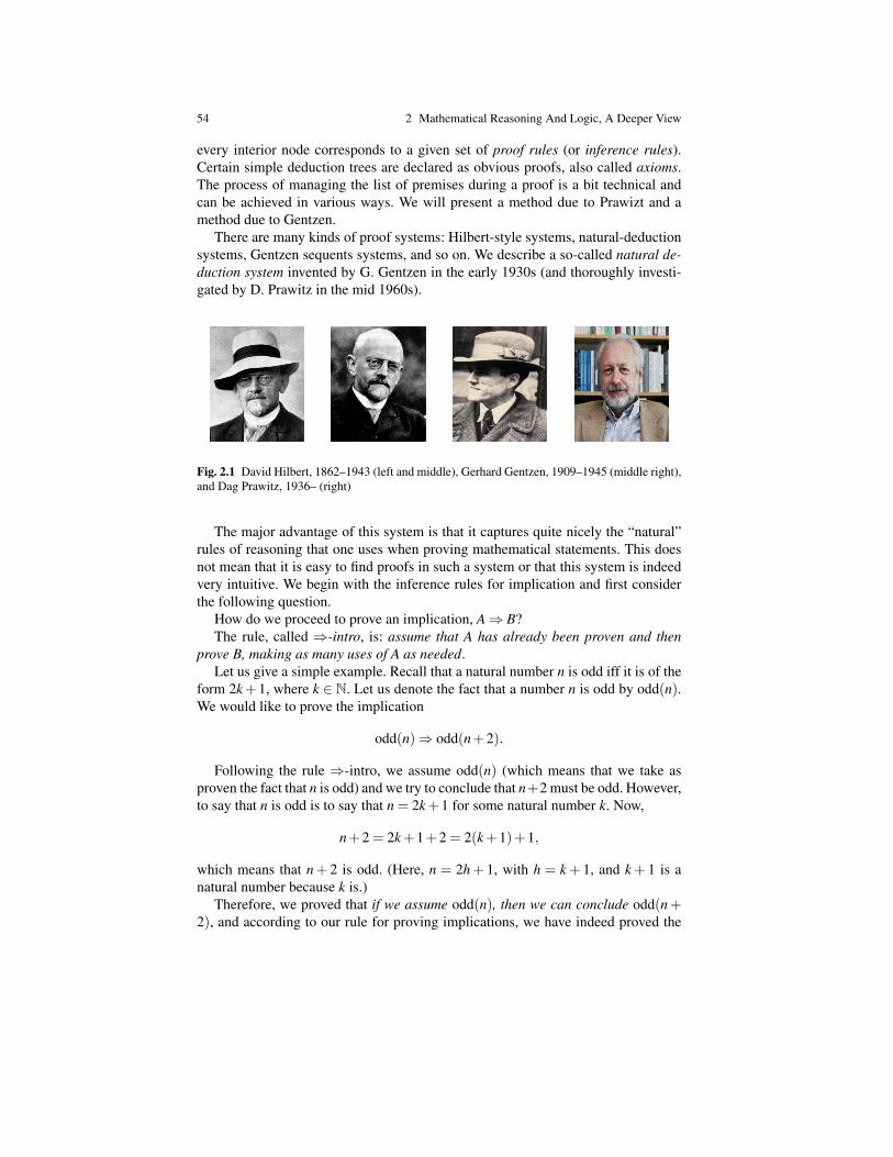
54 2 Mathematical Reasoning And Logic, A Deeper View
every interior node corresponds to a given set of proof rules (or inference rules).Certain simple deduction trees are declared as obvious proofs, also called axioms.The process of managing the list of premises during a proof is a bit technical andcan be achieved in various ways. We will present a method due to Prawizt and amethod due to Gentzen.
There are many kinds of proof systems: Hilbert-style systems, natural-deductionsystems, Gentzen sequents systems, and so on. We describe a so-called natural de-duction system invented by G. Gentzen in the early 1930s (and thoroughly investi-gated by D. Prawitz in the mid 1960s).
Fig. 2.1 David Hilbert, 1862–1943 (left and middle), Gerhard Gentzen, 1909–1945 (middle right),and Dag Prawitz, 1936– (right)
The major advantage of this system is that it captures quite nicely the “natural”rules of reasoning that one uses when proving mathematical statements. This doesnot mean that it is easy to find proofs in such a system or that this system is indeedvery intuitive. We begin with the inference rules for implication and first considerthe following question.
How do we proceed to prove an implication, A⇒ B?The rule, called ⇒-intro, is: assume that A has already been proven and then
prove B, making as many uses of A as needed.Let us give a simple example. Recall that a natural number n is odd iff it is of the
form 2k+1, where k ∈ N. Let us denote the fact that a number n is odd by odd(n).We would like to prove the implication
odd(n)⇒ odd(n+2).
Following the rule ⇒-intro, we assume odd(n) (which means that we take asproven the fact that n is odd) and we try to conclude that n+2 must be odd. However,to say that n is odd is to say that n = 2k+1 for some natural number k. Now,
n+2 = 2k+1+2 = 2(k+1)+1,
which means that n+ 2 is odd. (Here, n = 2h+ 1, with h = k + 1, and k + 1 is anatural number because k is.)
Therefore, we proved that if we assume odd(n), then we can conclude odd(n+2), and according to our rule for proving implications, we have indeed proved the

2.2 Inference Rules, Deductions, Proof Systems N ⇒m and N G⇒m 55
propositionodd(n)⇒ odd(n+2).
Note that the effect of rule ⇒-intro is to introduce the implication sign ⇒ be-tween the premise odd(n), which was temporarily assumed, and the conclusion ofthe deduction odd(n+2). This is why this rule is called the implication introduction.
It should be noted that the above proof of the proposition odd(n)⇒ odd(n+ 2)does not depend on any premises (other than the implicit fact that we are assumingn is a natural number). In particular, this proof does not depend on the premise,odd(n), which was assumed (became “active”) during our subproof step. Thus, afterhaving applied the rule⇒-intro, we should really make sure that the premise odd(n)which was made temporarily active is deactivated, or as we say, discharged. Whenwe write informal proofs, we rarely (if ever) explicitly discharge premises when weapply the rule⇒-intro but if we want to be rigorous we really should.
For a second example, we wish to prove the proposition P⇒ (Q⇒ P).According to our rule, we assume P as a premise and we try to prove Q⇒ P
assuming P. In order to prove Q⇒ P, we assume Q as a new premise so the set ofpremises becomes P,Q, and then we try to prove P from P and Q. This time, itshould be obvious that P is provable because we assumed both P and Q.
Indeed, the rule that P is always provable from any set of assumptions includingP itself is one of the basic axioms of our logic (which means that it is a rule thatrequires no justification whatsover). So, we have obtained a proof of P⇒ (Q⇒ P).
What is not entirely satisfactory about the above “proof” of P⇒ (Q⇒ P) isthat when the proof ends, the premises P and Q are still hanging around as “open”assumptions. However, a proof should not depend on any “open” assumptions andto rectify this problem we introduce a mechanism of “discharging” or “closing”premises, as we already suggested in our previous example.
What this means is that certain rules of our logic are required to discard (the usualterminology is “discharge”) certain occurrences of premises so that the resultingproof does not depend on these premises.
Technically, there are various ways of implementing the discharging mechanismbut they all involve some form of tagging (with a “new” variable). For example, therule formalizing the process that we have just described to prove an implication,A⇒ B, known as⇒-introduction, uses a tagging mechanism described precisely inDefinition 2.1.
Now, the rule that we have just described is not sufficient to prove certain propo-sitions that should be considered provable under the “standard” intuitive meaningof implication. For example, after a moment of thought, I think most people wouldwant the proposition P⇒ ((P⇒ Q)⇒ Q) to be provable. If we follow the proce-dure that we have advocated, we assume both P and P⇒ Q and we try to prove Q.For this, we need a new rule, namely:
If P and P⇒ Q are both provable, then Q is provable.The above rule is known as the⇒-elimination rule (or modus ponens) and it is
formalized in tree-form in Definition 2.1.
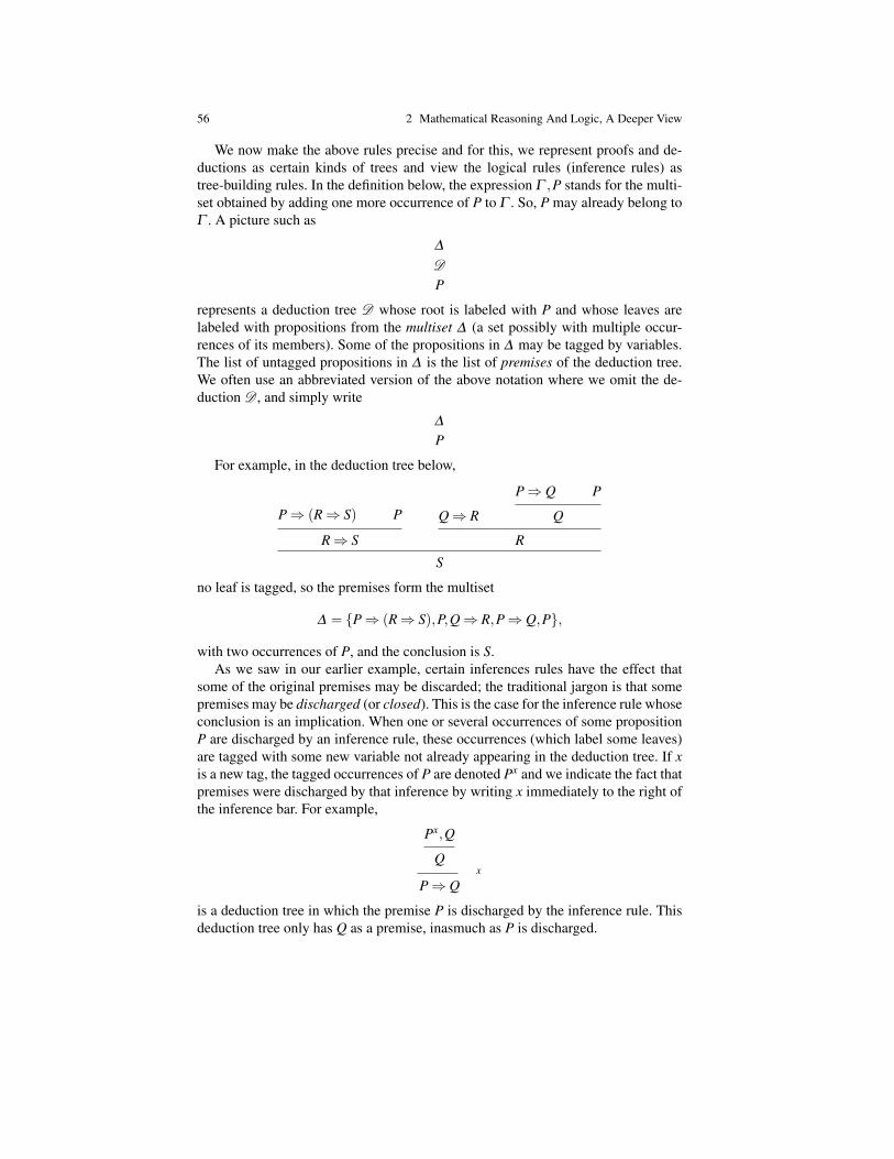
56 2 Mathematical Reasoning And Logic, A Deeper View
We now make the above rules precise and for this, we represent proofs and de-ductions as certain kinds of trees and view the logical rules (inference rules) astree-building rules. In the definition below, the expression Γ ,P stands for the multi-set obtained by adding one more occurrence of P to Γ . So, P may already belong toΓ . A picture such as
∆
D
P
represents a deduction tree D whose root is labeled with P and whose leaves arelabeled with propositions from the multiset ∆ (a set possibly with multiple occur-rences of its members). Some of the propositions in ∆ may be tagged by variables.The list of untagged propositions in ∆ is the list of premises of the deduction tree.We often use an abbreviated version of the above notation where we omit the de-duction D , and simply write
∆
P
For example, in the deduction tree below,
P⇒ (R⇒ S) P
R⇒ S
Q⇒ R
P⇒ Q P
Q
R
S
no leaf is tagged, so the premises form the multiset
∆ = P⇒ (R⇒ S),P,Q⇒ R,P⇒ Q,P,
with two occurrences of P, and the conclusion is S.As we saw in our earlier example, certain inferences rules have the effect that
some of the original premises may be discarded; the traditional jargon is that somepremises may be discharged (or closed). This is the case for the inference rule whoseconclusion is an implication. When one or several occurrences of some propositionP are discharged by an inference rule, these occurrences (which label some leaves)are tagged with some new variable not already appearing in the deduction tree. If xis a new tag, the tagged occurrences of P are denoted Px and we indicate the fact thatpremises were discharged by that inference by writing x immediately to the right ofthe inference bar. For example,
Px,Q
Qx
P⇒ Q
is a deduction tree in which the premise P is discharged by the inference rule. Thisdeduction tree only has Q as a premise, inasmuch as P is discharged.

2.2 Inference Rules, Deductions, Proof Systems N ⇒m and N G⇒m 57
What is the meaning of the horizontal bars? Actually, nothing really. Here, weare victims of an old habit in logic. Observe that there is always a single propositionimmediately under a bar but there may be several propositions immediately above abar. The intended meaning of the bar is that the proposition below it is obtained asthe result of applying an inference rule to the propositions above it. For example, in
Q⇒ R Q
R
the proposition R is the result of applying the ⇒-elimination rule (see Definition2.1 below) to the two premises Q⇒ R and Q. Thus, the use of the bar is just aconvention used by logicians going back at least to the 1900s. Removing the bareverywhere would not change anything in our trees, except perhaps reduce theirreadability. Most logic books draw proof trees using bars to indicate inferences,therefore we also use bars in depicting our proof trees.
Because propositions do not arise from the vacuum but instead are built up froma set of atomic propositions using logical connectives (here,⇒), we assume the ex-istence of an “official set of atomic propositions,” or set of propositional symbols,PS = P1,P2,P3, . . .. So, for example, P1 ⇒ P2 and P1 ⇒ (P2 ⇒ P1) are propo-sitions. Typically, we use upper-case letters such as P,Q,R,S,A,B,C, and so on, todenote arbitrary propositions formed using atoms from PS.
Definition 2.1. The axioms, inference rules, and deduction trees for implicationallogic are defined as follows.
Axioms.(i) Every one-node tree labeled with a single proposition P is a deduction tree for
P with set of premises P.(ii) The tree
Γ ,P
P
is a deduction tree for P with multiset set of premises Γ ,P.
The above is a concise way of denoting a two-node tree with its leaf labeled withthe multiset consisting of P and the propositions in Γ , each of these propositions(including P) having possibly multiple occurrences but at least one, and whose rootis labeled with P. A more explicit form is
k1︷ ︸︸ ︷P1, · · · ,P1, · · · ,
ki︷ ︸︸ ︷Pi, · · · ,Pi, · · · ,
kn︷ ︸︸ ︷Pn, · · · ,Pn ,
Pi
where k1, . . . ,kn ≥ 1 and n≥ 1. This axiom says that we always have a deduction ofPi from any set of premises including Pi.
The⇒-introduction rule.If D is a deduction tree for Q from the premises in Γ ,P, then
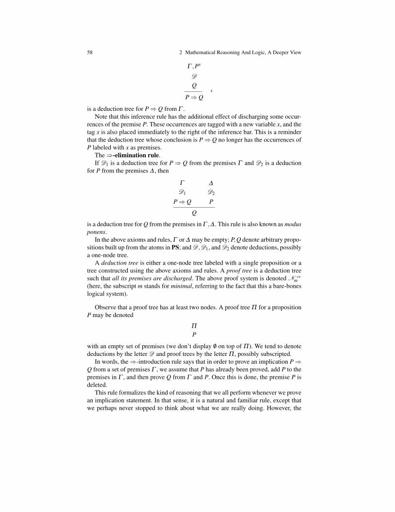
58 2 Mathematical Reasoning And Logic, A Deeper View
Γ ,Px
D
Qx
P⇒ Q
is a deduction tree for P⇒ Q from Γ .Note that this inference rule has the additional effect of discharging some occur-
rences of the premise P. These occurrences are tagged with a new variable x, and thetag x is also placed immediately to the right of the inference bar. This is a reminderthat the deduction tree whose conclusion is P⇒Q no longer has the occurrences ofP labeled with x as premises.
The⇒-elimination rule.If D1 is a deduction tree for P⇒ Q from the premises Γ and D2 is a deduction
for P from the premises ∆ , then
Γ
D1
P⇒ Q
∆
D2
P
Q
is a deduction tree for Q from the premises in Γ ,∆ . This rule is also known as modusponens.
In the above axioms and rules, Γ or ∆ may be empty; P,Q denote arbitrary propo-sitions built up from the atoms in PS; and D ,D1, and D2 denote deductions, possiblya one-node tree.
A deduction tree is either a one-node tree labeled with a single proposition or atree constructed using the above axioms and rules. A proof tree is a deduction treesuch that all its premises are discharged. The above proof system is denoted N ⇒
m(here, the subscript m stands for minimal, referring to the fact that this a bare-boneslogical system).
Observe that a proof tree has at least two nodes. A proof tree Π for a propositionP may be denoted
Π
P
with an empty set of premises (we don’t display /0 on top of Π ). We tend to denotedeductions by the letter D and proof trees by the letter Π , possibly subscripted.
In words, the⇒-introduction rule says that in order to prove an implication P⇒Q from a set of premises Γ , we assume that P has already been proved, add P to thepremises in Γ , and then prove Q from Γ and P. Once this is done, the premise P isdeleted.
This rule formalizes the kind of reasoning that we all perform whenever we provean implication statement. In that sense, it is a natural and familiar rule, except thatwe perhaps never stopped to think about what we are really doing. However, the
2.2 Inference Rules, Deductions, Proof Systems N ⇒m and N G⇒m 59
business about discharging the premise P when we are through with our argumentis a bit puzzling. Most people probably never carry out this “discharge step” con-sciously, but such a process does take place implicitly.
It might help to view the action of proving an implication P⇒Q as the construc-tion of a program that converts a proof of P into a proof of Q. Then, if we supply aproof of P as input to this program (the proof of P⇒Q), it will output a proof of Q.So, if we don’t give the right kind of input to this program, for example, a “wrongproof” of P, we should not expect the program to return a proof of Q. However, thisdoes not say that the program is incorrect; the program was designed to do the rightthing only if it is given the right kind of input. From this functional point of view(also called constructive), if we take the simplistic view that P and Q assume thetruth values true and false, we should not be shocked that if we give as input thevalue false (for P), then the truth value of the whole implication P⇒Q is true. Theprogram P⇒Q is designed to produce the output value true (for Q) if it is given theinput value true (for P). So, this program only goes wrong when, given the inputtrue (for P), it returns the value false (for Q). In this erroneous case, P⇒ Q shouldindeed receive the value false. However, in all other cases, the program works cor-rectly, even if it is given the wrong input (false for P).
For a concrete example, say P stands for the statement,“Our candidate for president wins in Pennsylvania”and Q stands for“Our candidate is elected president.”Then, P⇒ Q, asserts that if our candidate for president wins in Pennsylvania
then our candidate is elected president.If P⇒ Q holds, then if indeed our candidate for president wins in Pennsylvania
then for sure our candidate will win the presidential election. However, if our candi-date does not win in Pennsylvania, we can’t predict what will happen. Our candidatemay still win the presidential election but he may not.
If our candidate president does not win in Pennsylvania, our prediction is notproven false. In this case, the statement P ⇒ Q should be regarded as holding,though perhaps uninteresting.
For one more example, let odd(n) assert that n is an odd natural number and letQ(n,a,b) assert that an + bn is divisible by a+ b, where a,b are any given naturalnumbers. By divisible, we mean that we can find some natural number c, so that
an +bn = (a+b)c.
Then, we claim that the implication odd(n)⇒ Q(n,a,b) is provable.As usual, let us assume odd(n), so that n = 2k+ 1, where k = 0,1,2,3, . . .. But
then, we can easily check that
a2k+1 +b2k+1 = (a+b)
(2k
∑i=0
(−1)ia2k−ibi
),
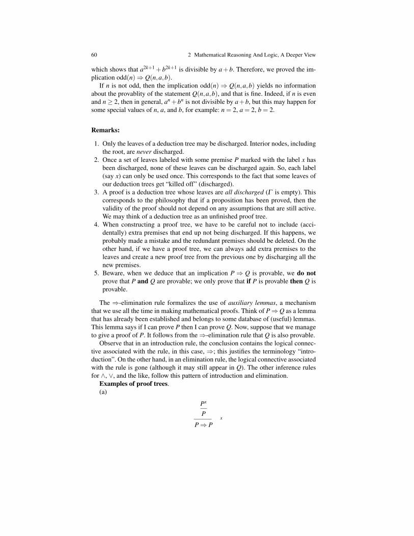
60 2 Mathematical Reasoning And Logic, A Deeper View
which shows that a2k+1 +b2k+1 is divisible by a+b. Therefore, we proved the im-plication odd(n)⇒ Q(n,a,b).
If n is not odd, then the implication odd(n)⇒ Q(n,a,b) yields no informationabout the provablity of the statement Q(n,a,b), and that is fine. Indeed, if n is evenand n≥ 2, then in general, an +bn is not divisible by a+b, but this may happen forsome special values of n, a, and b, for example: n = 2, a = 2, b = 2.
Remarks:
1. Only the leaves of a deduction tree may be discharged. Interior nodes, includingthe root, are never discharged.
2. Once a set of leaves labeled with some premise P marked with the label x hasbeen discharged, none of these leaves can be discharged again. So, each label(say x) can only be used once. This corresponds to the fact that some leaves ofour deduction trees get “killed off” (discharged).
3. A proof is a deduction tree whose leaves are all discharged (Γ is empty). Thiscorresponds to the philosophy that if a proposition has been proved, then thevalidity of the proof should not depend on any assumptions that are still active.We may think of a deduction tree as an unfinished proof tree.
4. When constructing a proof tree, we have to be careful not to include (acci-dentally) extra premises that end up not being discharged. If this happens, weprobably made a mistake and the redundant premises should be deleted. On theother hand, if we have a proof tree, we can always add extra premises to theleaves and create a new proof tree from the previous one by discharging all thenew premises.
5. Beware, when we deduce that an implication P⇒ Q is provable, we do notprove that P and Q are provable; we only prove that if P is provable then Q isprovable.
The ⇒-elimination rule formalizes the use of auxiliary lemmas, a mechanismthat we use all the time in making mathematical proofs. Think of P⇒Q as a lemmathat has already been established and belongs to some database of (useful) lemmas.This lemma says if I can prove P then I can prove Q. Now, suppose that we manageto give a proof of P. It follows from the⇒-elimination rule that Q is also provable.
Observe that in an introduction rule, the conclusion contains the logical connec-tive associated with the rule, in this case, ⇒; this justifies the terminology “intro-duction”. On the other hand, in an elimination rule, the logical connective associatedwith the rule is gone (although it may still appear in Q). The other inference rulesfor ∧, ∨, and the like, follow this pattern of introduction and elimination.
Examples of proof trees.(a)
Px
Px
P⇒ P
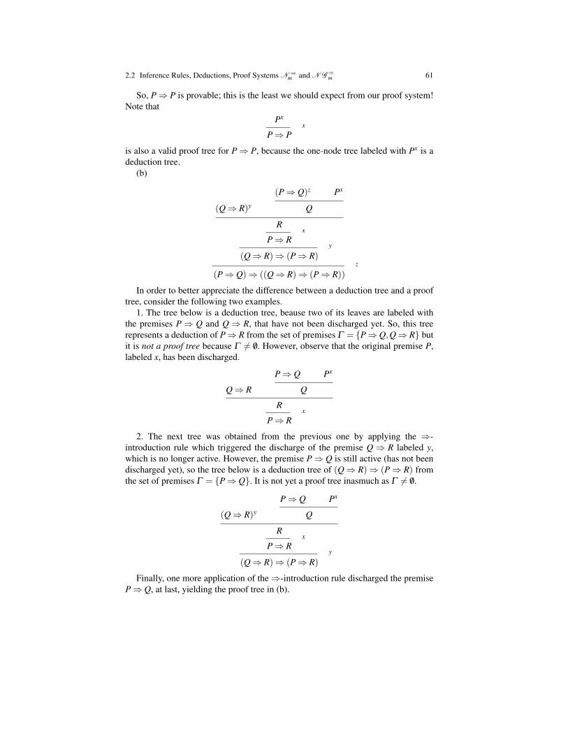
2.2 Inference Rules, Deductions, Proof Systems N ⇒m and N G⇒m 61
So, P⇒ P is provable; this is the least we should expect from our proof system!Note that
Pxx
P⇒ P
is also a valid proof tree for P⇒ P, because the one-node tree labeled with Px is adeduction tree.
(b)
(Q⇒ R)y
(P⇒ Q)z Px
Q
Rx
P⇒ Ry
(Q⇒ R)⇒ (P⇒ R)z
(P⇒ Q)⇒ ((Q⇒ R)⇒ (P⇒ R))
In order to better appreciate the difference between a deduction tree and a prooftree, consider the following two examples.
1. The tree below is a deduction tree, beause two of its leaves are labeled withthe premises P⇒ Q and Q⇒ R, that have not been discharged yet. So, this treerepresents a deduction of P⇒ R from the set of premises Γ = P⇒Q,Q⇒ R butit is not a proof tree because Γ 6= /0. However, observe that the original premise P,labeled x, has been discharged.
Q⇒ R
P⇒ Q Px
Q
Rx
P⇒ R
2. The next tree was obtained from the previous one by applying the ⇒-introduction rule which triggered the discharge of the premise Q⇒ R labeled y,which is no longer active. However, the premise P⇒ Q is still active (has not beendischarged yet), so the tree below is a deduction tree of (Q⇒ R)⇒ (P⇒ R) fromthe set of premises Γ = P⇒ Q. It is not yet a proof tree inasmuch as Γ 6= /0.
(Q⇒ R)y
P⇒ Q Px
Q
Rx
P⇒ Ry
(Q⇒ R)⇒ (P⇒ R)
Finally, one more application of the⇒-introduction rule discharged the premiseP⇒ Q, at last, yielding the proof tree in (b).
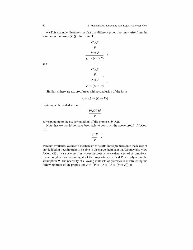
62 2 Mathematical Reasoning And Logic, A Deeper View
(c) This example illustrates the fact that different proof trees may arise from thesame set of premises P,Q: for example,
Px,Qy
Px
P⇒ Py
Q⇒ (P⇒ P)
and
Px,Qy
Py
Q⇒ Px
P⇒ (Q⇒ P)
Similarly, there are six proof trees with a conclusion of the form
A⇒ (B⇒ (C⇒ P))
begining with the deduction
Px,Qy,Rz
P
corresponding to the six permutations of the premises P,Q,R.Note that we would not have been able to construct the above proofs if Axiom
(ii),
Γ ,P,
P
were not available. We need a mechanism to “stuff” more premises into the leaves ofour deduction trees in order to be able to discharge them later on. We may also viewAxiom (ii) as a weakening rule whose purpose is to weaken a set of assumptions.Even though we are assuming all of the proposition in Γ and P, we only retain theassumption P. The necessity of allowing multisets of premises is illustrated by thefollowing proof of the proposition P⇒ (P⇒ (Q⇒ (Q⇒ (P⇒ P)))):

2.2 Inference Rules, Deductions, Proof Systems N ⇒m and N G⇒m 63
Pu,Pv,Py,Qw,Qx
Py
P⇒ Px
Q⇒ (P⇒ P)w
Q⇒ (Q⇒ (P⇒ P))v
P⇒ (Q⇒ (Q⇒ (P⇒ P)))u
P⇒ (P⇒ (Q⇒ (Q⇒ (P⇒ P))))
(d) In the next example, the two occurrences of A labeled x are discharged simul-taneously.
(A⇒ (B⇒C))z Ax
B⇒C
(A⇒ B)y Ax
B
Cx
A⇒Cy
(A⇒ B)⇒ (A⇒C)z(
A⇒ (B⇒C))⇒((A⇒ B)⇒ (A⇒C)
)(e) In contrast to Example (d), in the proof tree below the two occurrences of A
are discharged separately. To this effect, they are labeled differently.
(A⇒ (B⇒C))z Ax
B⇒C
(A⇒ B)y At
B
Cx
A⇒Cy
(A⇒ B)⇒ (A⇒C)z(
A⇒ (B⇒C))⇒((A⇒ B)⇒ (A⇒C)
)t
A⇒((
A⇒ (B⇒C))⇒((A⇒ B)⇒ (A⇒C)
))Remark: How do we find these proof trees? Well, we could try to enumerate allpossible proof trees systematically and see if a proof of the desired conclusion turnsup. Obviously, this is a very inefficient procedure and moreover, how do we knowthat all possible proof trees will be generated and how do we know that such amethod will terminate after a finite number of steps (what if the proposition pro-posed as a conclusion of a proof is not provable)?
Finding an algorithm to decide whether a proposition is provable is a very dif-ficult problem and, for sets of propositions with enough “expressive power” (such
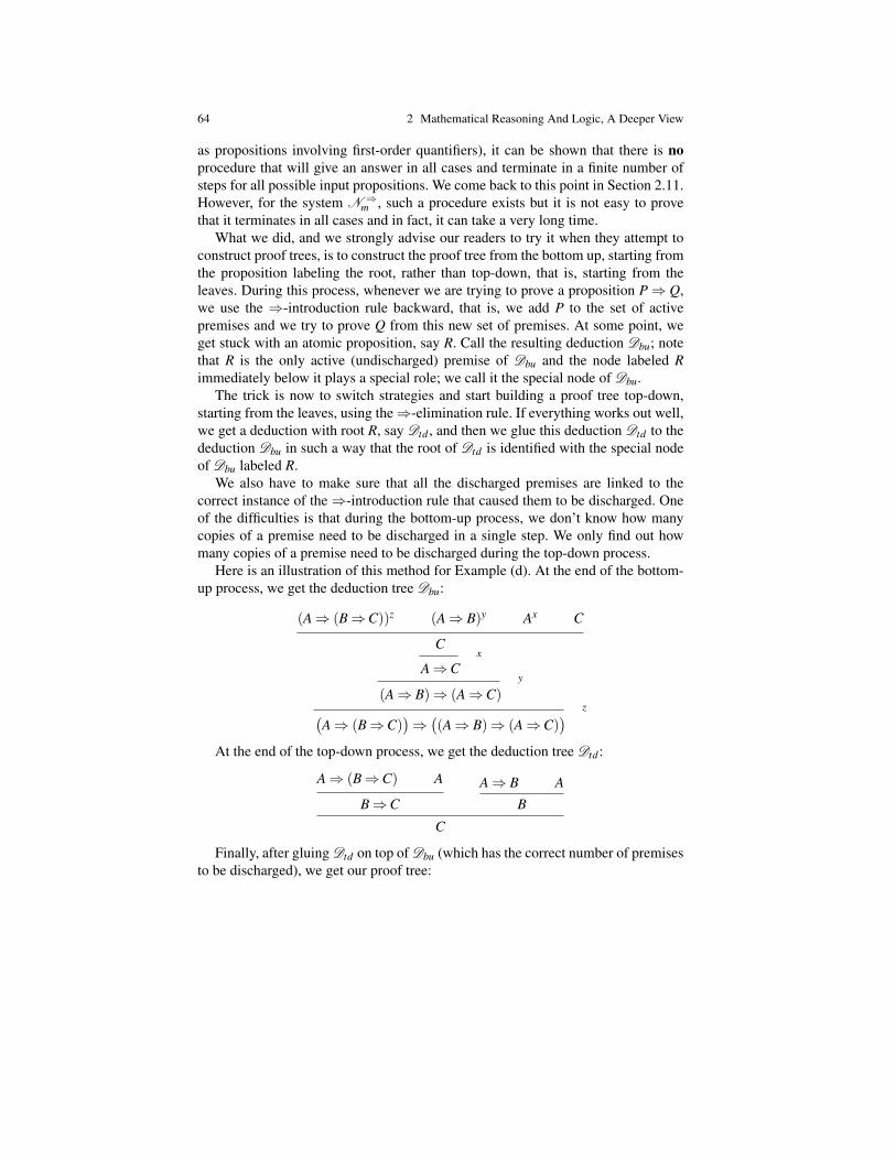
64 2 Mathematical Reasoning And Logic, A Deeper View
as propositions involving first-order quantifiers), it can be shown that there is noprocedure that will give an answer in all cases and terminate in a finite number ofsteps for all possible input propositions. We come back to this point in Section 2.11.However, for the system N ⇒
m , such a procedure exists but it is not easy to provethat it terminates in all cases and in fact, it can take a very long time.
What we did, and we strongly advise our readers to try it when they attempt toconstruct proof trees, is to construct the proof tree from the bottom up, starting fromthe proposition labeling the root, rather than top-down, that is, starting from theleaves. During this process, whenever we are trying to prove a proposition P⇒ Q,we use the ⇒-introduction rule backward, that is, we add P to the set of activepremises and we try to prove Q from this new set of premises. At some point, weget stuck with an atomic proposition, say R. Call the resulting deduction Dbu; notethat R is the only active (undischarged) premise of Dbu and the node labeled Rimmediately below it plays a special role; we call it the special node of Dbu.
The trick is now to switch strategies and start building a proof tree top-down,starting from the leaves, using the⇒-elimination rule. If everything works out well,we get a deduction with root R, say Dtd , and then we glue this deduction Dtd to thededuction Dbu in such a way that the root of Dtd is identified with the special nodeof Dbu labeled R.
We also have to make sure that all the discharged premises are linked to thecorrect instance of the⇒-introduction rule that caused them to be discharged. Oneof the difficulties is that during the bottom-up process, we don’t know how manycopies of a premise need to be discharged in a single step. We only find out howmany copies of a premise need to be discharged during the top-down process.
Here is an illustration of this method for Example (d). At the end of the bottom-up process, we get the deduction tree Dbu:
(A⇒ (B⇒C))z (A⇒ B)y Ax C
Cx
A⇒Cy
(A⇒ B)⇒ (A⇒C)z(
A⇒ (B⇒C))⇒((A⇒ B)⇒ (A⇒C)
)At the end of the top-down process, we get the deduction tree Dtd :
A⇒ (B⇒C) A
B⇒CA⇒ B A
B
C
Finally, after gluing Dtd on top of Dbu (which has the correct number of premisesto be discharged), we get our proof tree:
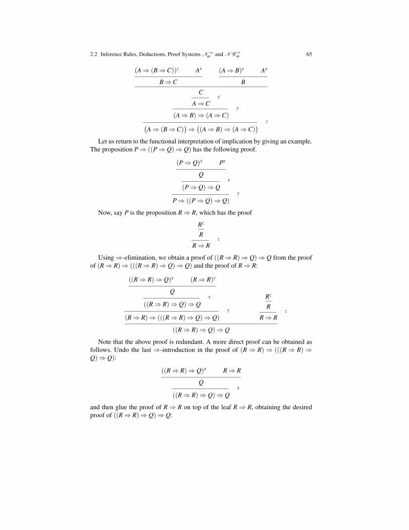
2.2 Inference Rules, Deductions, Proof Systems N ⇒m and N G⇒m 65
(A⇒ (B⇒C))z Ax
B⇒C
(A⇒ B)y Ax
B
Cx
A⇒Cy
(A⇒ B)⇒ (A⇒C)z(
A⇒ (B⇒C))⇒((A⇒ B)⇒ (A⇒C)
)Let us return to the functional interpretation of implication by giving an example.
The proposition P⇒ ((P⇒ Q)⇒ Q) has the following proof.
(P⇒ Q)x Py
Qx
(P⇒ Q)⇒ Qy
P⇒ ((P⇒ Q)⇒ Q)
Now, say P is the proposition R⇒ R, which has the proof
Rz
Rz
R⇒ R
Using⇒-elimination, we obtain a proof of ((R⇒ R)⇒ Q)⇒ Q from the proofof (R⇒ R)⇒ (((R⇒ R)⇒ Q)⇒ Q) and the proof of R⇒ R:
((R⇒ R)⇒ Q)x (R⇒ R)y
Qx
((R⇒ R)⇒ Q)⇒ Qy
(R⇒ R)⇒ (((R⇒ R)⇒ Q)⇒ Q)
Rz
Rz
R⇒ R
((R⇒ R)⇒ Q)⇒ Q
Note that the above proof is redundant. A more direct proof can be obtained asfollows. Undo the last ⇒-introduction in the proof of (R⇒ R)⇒ (((R⇒ R)⇒Q)⇒ Q):
((R⇒ R)⇒ Q)x R⇒ R
Qx
((R⇒ R)⇒ Q)⇒ Q
and then glue the proof of R⇒ R on top of the leaf R⇒ R, obtaining the desiredproof of ((R⇒ R)⇒ Q)⇒ Q:

66 2 Mathematical Reasoning And Logic, A Deeper View
((R⇒ R)⇒ Q)x
Rz
Rz
R⇒ R
Qx
((R⇒ R)⇒ Q)⇒ Q
In general, one has to exercise care with the label variables. It may be necessary torename some of these variables to avoid clashes. What we have above is an exampleof proof substitution also called proof normalization. We come back to this topic inSection 2.11.
The process of discharging premises when constructing a deduction is admittedlya bit confusing. Part of the problem is that a deduction tree really represents the lastof a sequence of stages (corresponding to the application of inference rules) duringwhich the current set of “active” premises, that is, those premises that have not yetbeen discharged (closed, cancelled) evolves (in fact, shrinks). Some mechanism isneeded to keep track of which premises are no longer active and this is what thisbusiness of labeling premises with variables achieves. Historically, this is the firstmechanism that was invented. However, Gentzen (in the 1930s) came up with analternative solution that is mathematically easier to handle. Moreover, it turns outthat this notation is also better suited to computer implementations, if one wishes toimplement an automated theorem prover.
The point is to keep a record of all undischarged assumptions at every stage of thededuction. Thus, a deduction is now a tree whose nodes are labeled with expressionsof the form Γ → P, called sequents, where P is a proposition, and Γ is a record ofall undischarged assumptions at the stage of the deduction associated with this node.
During the construction of a deduction tree, it is necessary to discharge packetsof assumptions consisting of one or more occurrences of the same proposition. Tothis effect, it is convenient to tag packets of assumptions with labels, in order todischarge the propositions in these packets in a single step. We use variables for thelabels, and a packet labeled with x consisting of occurrences of the proposition P iswritten as x : P. Thus, in a sequent Γ → P, the expression Γ is any finite set of theform x1 : P1, . . . ,xm : Pm, where the xi are pairwise distinct (but the Pi need not be dis-tinct). Given Γ = x1 : P1, . . . ,xm : Pm, the notation Γ ,x : P is only well defined whenx 6= xi for all i, 1≤ i≤ m, in which case it denotes the set x1 : P1, . . . ,xm : Pm,x : P.
Using sequents, the axioms and rules of Definition 2.2 are now expressed asfollows.
Definition 2.2. The axioms and inference rules of the system N G⇒m (implicationallogic, Gentzen-sequent style (the G in N G stands for Gentzen)) are listed below:
Γ ,x : P→ P (Axioms)
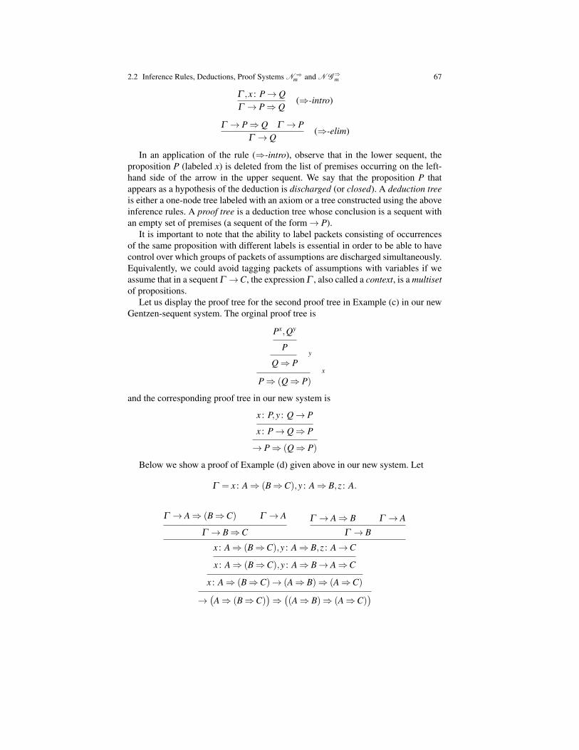
2.2 Inference Rules, Deductions, Proof Systems N ⇒m and N G⇒m 67
Γ ,x : P→ QΓ → P⇒ Q
(⇒-intro)
Γ → P⇒ Q Γ → PΓ → Q
(⇒-elim)
In an application of the rule (⇒-intro), observe that in the lower sequent, theproposition P (labeled x) is deleted from the list of premises occurring on the left-hand side of the arrow in the upper sequent. We say that the proposition P thatappears as a hypothesis of the deduction is discharged (or closed). A deduction treeis either a one-node tree labeled with an axiom or a tree constructed using the aboveinference rules. A proof tree is a deduction tree whose conclusion is a sequent withan empty set of premises (a sequent of the form→ P).
It is important to note that the ability to label packets consisting of occurrencesof the same proposition with different labels is essential in order to be able to havecontrol over which groups of packets of assumptions are discharged simultaneously.Equivalently, we could avoid tagging packets of assumptions with variables if weassume that in a sequent Γ →C, the expression Γ , also called a context, is a multisetof propositions.
Let us display the proof tree for the second proof tree in Example (c) in our newGentzen-sequent system. The orginal proof tree is
Px,Qy
Py
Q⇒ Px
P⇒ (Q⇒ P)
and the corresponding proof tree in our new system is
x : P,y : Q→ P
x : P→ Q⇒ P
→ P⇒ (Q⇒ P)
Below we show a proof of Example (d) given above in our new system. Let
Γ = x : A⇒ (B⇒C),y : A⇒ B,z : A.
Γ → A⇒ (B⇒C) Γ → A
Γ → B⇒C
Γ → A⇒ B Γ → A
Γ → B
x : A⇒ (B⇒C),y : A⇒ B,z : A→C
x : A⇒ (B⇒C),y : A⇒ B→ A⇒C
x : A⇒ (B⇒C)→ (A⇒ B)⇒ (A⇒C)
→(A⇒ (B⇒C)
)⇒((A⇒ B)⇒ (A⇒C)
)

68 2 Mathematical Reasoning And Logic, A Deeper View
Remark: An attentive reader will have surely noticed that the second version of the⇒-elimination rule,
Γ → P⇒ Q Γ → PΓ → Q
(⇒-elim),
differs slightly from the first version given in Definition 2.1. Indeed, in Prawitz’sstyle, the rule that matches exactly the⇒-elim rule above is
Γ
D1
P⇒ Q
Γ
D2
P
Q
where the deductions of P⇒ Q and P have the same set of premises, Γ . Equiv-alently, the rule in sequent format that corresponds to the ⇒-elimination rule ofDefinition 2.1 is
Γ → P⇒ Q ∆ → PΓ ,∆ → Q
(⇒-elim’),
where Γ ,∆ must be interpreted as the union of Γ and ∆ .A moment of reflection will reveal that the resulting proof systems are equivalent
(i.e., every proof in one system can be converted to a proof in the other system andvice versa); if you are not sure, do Problem 2.15. The version of the⇒-eliminationrule in Definition 2.1 may be considered preferable because it gives us the abilityto make the sets of premises labeling leaves smaller. On the other hand, after ex-perimenting with the construction of proofs, one gets the feeling that every proofcan be simplified to a “unique minimal” proof, if we define “minimal” in a suitablesense, namely, that a minimal proof never contains an elimination rule immediatelyfollowing an introduction rule (for more on this, see Section 2.11). Then, it turns outthat to define the notion of uniqueness of proofs, the second version is preferable.However, it is important to realize that in general, a proposition may possess distinctminimal proofs.
In principle, it does not matter which of the two systems N ⇒m or N G⇒m we use to
construct deductions; it is basically a matter of taste. The Prawitz-style system N ⇒m
produces proofs that are closer to the informal proofs that humans construct. Onethe other hand, the Gentzen-style system N G⇒m is better suited for implementingtheorem provers. My experience is that I make fewer mistakes with the Gentzen-sequent style system N G⇒m .
We now describe the inference rules dealing with the connectives ∧, ∨ and ⊥.
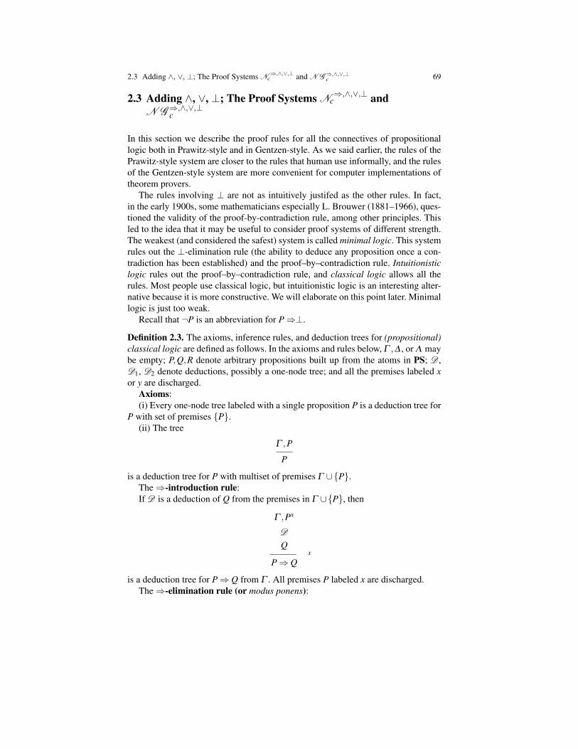
2.3 Adding ∧, ∨, ⊥; The Proof Systems N ⇒,∧,∨,⊥c and N G⇒,∧,∨,⊥
c 69
2.3 Adding ∧, ∨, ⊥; The Proof Systems N ⇒,∧,∨,⊥c and
N G⇒,∧,∨,⊥c
In this section we describe the proof rules for all the connectives of propositionallogic both in Prawitz-style and in Gentzen-style. As we said earlier, the rules of thePrawitz-style system are closer to the rules that human use informally, and the rulesof the Gentzen-style system are more convenient for computer implementations oftheorem provers.
The rules involving ⊥ are not as intuitively justifed as the other rules. In fact,in the early 1900s, some mathematicians especially L. Brouwer (1881–1966), ques-tioned the validity of the proof-by-contradiction rule, among other principles. Thisled to the idea that it may be useful to consider proof systems of different strength.The weakest (and considered the safest) system is called minimal logic. This systemrules out the ⊥-elimination rule (the ability to deduce any proposition once a con-tradiction has been established) and the proof–by–contradiction rule. Intuitionisticlogic rules out the proof–by–contradiction rule, and classical logic allows all therules. Most people use classical logic, but intuitionistic logic is an interesting alter-native because it is more constructive. We will elaborate on this point later. Minimallogic is just too weak.
Recall that ¬P is an abbreviation for P⇒⊥.
Definition 2.3. The axioms, inference rules, and deduction trees for (propositional)classical logic are defined as follows. In the axioms and rules below, Γ ,∆ , or Λ maybe empty; P,Q,R denote arbitrary propositions built up from the atoms in PS; D ,D1, D2 denote deductions, possibly a one-node tree; and all the premises labeled xor y are discharged.
Axioms:(i) Every one-node tree labeled with a single proposition P is a deduction tree for
P with set of premises P.(ii) The tree
Γ ,P
P
is a deduction tree for P with multiset of premises Γ ∪P.The⇒-introduction rule:If D is a deduction of Q from the premises in Γ ∪P, then
Γ ,Px
D
Qx
P⇒ Q
is a deduction tree for P⇒ Q from Γ . All premises P labeled x are discharged.The⇒-elimination rule (or modus ponens):
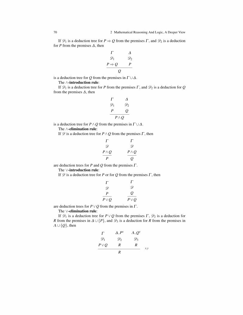
70 2 Mathematical Reasoning And Logic, A Deeper View
If D1 is a deduction tree for P⇒ Q from the premises Γ , and D2 is a deductionfor P from the premises ∆ , then
Γ
D1
P⇒ Q
∆
D2
P
Q
is a deduction tree for Q from the premises in Γ ∪∆ .The ∧-introduction rule:If D1 is a deduction tree for P from the premises Γ , and D2 is a deduction for Q
from the premises ∆ , then
Γ
D1
P
∆
D2
Q
P∧Q
is a deduction tree for P∧Q from the premises in Γ ∪∆ .The ∧-elimination rule:If D is a deduction tree for P∧Q from the premises Γ , then
Γ
D
P∧Q
P
Γ
D
P∧Q
Q
are deduction trees for P and Q from the premises Γ .The ∨-introduction rule:If D is a deduction tree for P or for Q from the premises Γ , then
Γ
D
P
P∨Q
Γ
D
Q
P∨Q
are deduction trees for P∨Q from the premises in Γ .The ∨-elimination rule:If D1 is a deduction tree for P∨Q from the premises Γ , D2 is a deduction for
R from the premises in ∆ ∪P, and D3 is a deduction for R from the premises inΛ ∪Q, then
Γ
D1
P∨Q
∆ ,Px
D2
R
Λ ,Qy
D3
Rx,y
R

2.3 Adding ∧, ∨, ⊥; The Proof Systems N ⇒,∧,∨,⊥c and N G⇒,∧,∨,⊥
c 71
is a deduction tree for R from the premises in Γ ∪∆ ∪Λ . All premises P labeled xand all premises Q labeled y are discharged.
The ⊥-elimination rule:If D is a deduction tree for ⊥ from the premises Γ , then
Γ
D
⊥P
is a deduction tree for P from the premises Γ , for any proposition P.The proof–by–contradiction rule (also known as reductio ad absurdum rule,
for short RAA):If D is a deduction tree for ⊥ from the premises in Γ ∪¬P, then
Γ ,¬Px
D
⊥x
P
is a deduction tree for P from the premises Γ . All premises ¬P labeled x, are dis-charged.
Because ¬P is an abbreviation for P⇒⊥, the ¬-introduction rule is a special caseof the⇒-introduction rule (with Q =⊥). However, it is worth stating it explicitly.
The ¬-introduction rule:If D is a deduction tree for ⊥ from the premises in Γ ∪P, then
Γ ,Px
D
⊥x
¬P
is a deduction tree for ¬P from the premises Γ . All premises P labeled x, are dis-charged.
The above rule can be viewed as a proof–by–contradiction principle applied tonegated propositions.
Similarly, the ¬-elimination rule is a special case of⇒-elimination applied to¬P (= P⇒⊥) and P.
The ¬-elimination rule:If D1 is a deduction tree for ¬P from the premises Γ , and D2 is a deduction for
P from the premises ∆ , then
Γ
D1
¬P
∆
D2
P
⊥
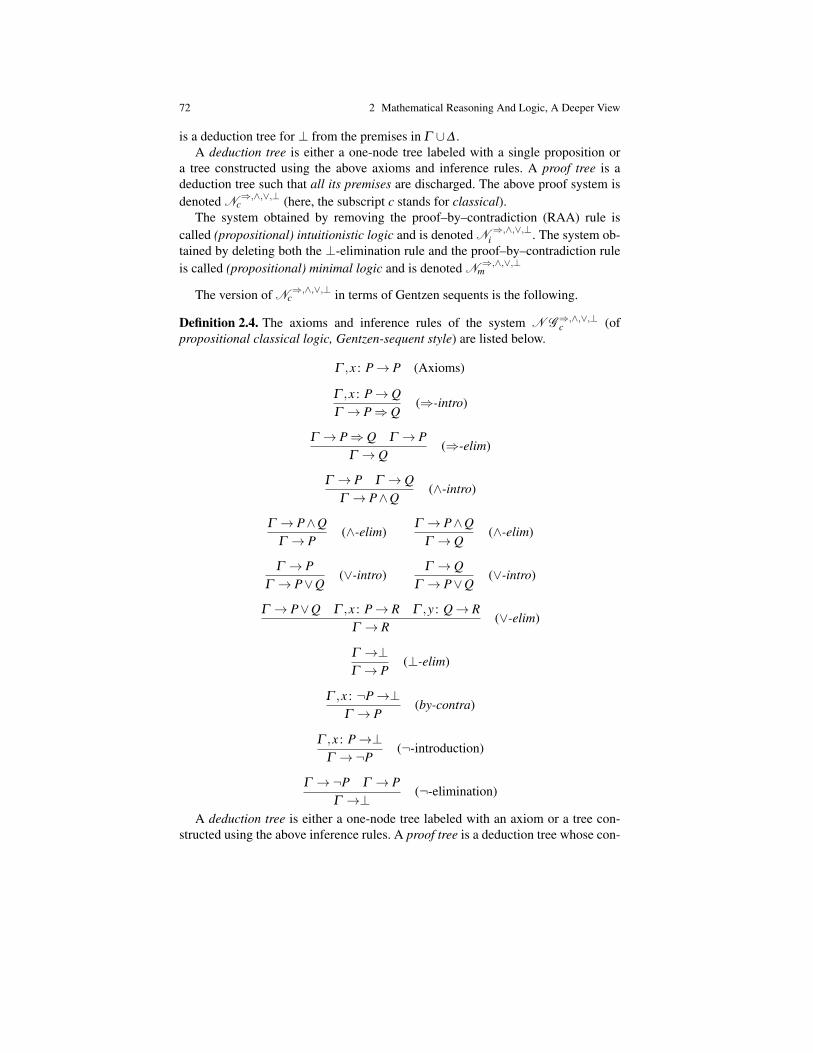
72 2 Mathematical Reasoning And Logic, A Deeper View
is a deduction tree for ⊥ from the premises in Γ ∪∆ .A deduction tree is either a one-node tree labeled with a single proposition or
a tree constructed using the above axioms and inference rules. A proof tree is adeduction tree such that all its premises are discharged. The above proof system isdenoted N ⇒,∧,∨,⊥
c (here, the subscript c stands for classical).The system obtained by removing the proof–by–contradiction (RAA) rule is
called (propositional) intuitionistic logic and is denoted N ⇒,∧,∨,⊥i . The system ob-
tained by deleting both the ⊥-elimination rule and the proof–by–contradiction ruleis called (propositional) minimal logic and is denoted N ⇒,∧,∨,⊥
m
The version of N ⇒,∧,∨,⊥c in terms of Gentzen sequents is the following.
Definition 2.4. The axioms and inference rules of the system N G⇒,∧,∨,⊥c (of
propositional classical logic, Gentzen-sequent style) are listed below.
Γ ,x : P→ P (Axioms)
Γ ,x : P→ QΓ → P⇒ Q
(⇒-intro)
Γ → P⇒ Q Γ → PΓ → Q
(⇒-elim)
Γ → P Γ → QΓ → P∧Q
(∧-intro)
Γ → P∧QΓ → P
(∧-elim)Γ → P∧Q
Γ → Q(∧-elim)
Γ → PΓ → P∨Q
(∨-intro)Γ → Q
Γ → P∨Q(∨-intro)
Γ → P∨Q Γ ,x : P→ R Γ ,y : Q→ RΓ → R
(∨-elim)
Γ →⊥Γ → P
(⊥-elim)
Γ ,x : ¬P→⊥Γ → P
(by-contra)
Γ ,x : P→⊥Γ →¬P
(¬-introduction)
Γ →¬P Γ → PΓ →⊥ (¬-elimination)
A deduction tree is either a one-node tree labeled with an axiom or a tree con-structed using the above inference rules. A proof tree is a deduction tree whose con-

2.3 Adding ∧, ∨, ⊥; The Proof Systems N ⇒,∧,∨,⊥c and N G⇒,∧,∨,⊥
c 73
clusion is a sequent with an empty set of premises (a sequent of the form /0→ P).
The rule (⊥-elim) is trivial (does nothing) when P=⊥, therefore from now on weassume that P 6=⊥. Propositional minimal logic, denoted N G⇒,∧,∨,⊥
m , is obtainedby dropping the (⊥-elim) and (by-contra) rules. Propositional intuitionistic logic,denoted N G⇒,∧,∨,⊥
i , is obtained by dropping the (by-contra) rule.
When we say that a proposition P is provable from Γ , we mean that we canconstruct a proof tree whose conclusion is P and whose set of premises is Γ , inone of the systems N ⇒,∧,∨,⊥
c or N G⇒,∧,∨,⊥c . Therefore, when we use the word
“provable” unqualified, we mean provable in classical logic. If P is provable fromΓ in one of the intuitionistic systems N ⇒,∧,∨,⊥
i or N G⇒,∧,∨,⊥i , then we say intu-
itionistically provable (and similarly, if P is provable from Γ in one of the systemsN ⇒,∧,∨,⊥
m or N G⇒,∧,∨,⊥m , then we say provable in minimal logic). When P is prov-
able from Γ , most people write Γ ` P, or `Γ → P, sometimes with the name of thecorresponding proof system tagged as a subscript on the sign ` if necessary to avoidambiguities. When Γ is empty, we just say P is provable (provable in intuitionisticlogic, and so on) and write ` P.
We treat logical equivalence as a derived connective: that is, we view P ≡ Q asan abbreviation for (P⇒Q)∧ (Q⇒ P). In view of the inference rules for ∧, we seethat to prove a logical equivalence P ≡ Q, we just have to prove both implicationsP⇒ Q and Q⇒ P.
Since the only difference between the proof systems N ⇒,∧,∨,⊥m and N G⇒,∧,∨,⊥
mis the way in which they perform the bookkeeping of premises, it is intuitively clearthat they are equivalent. However, they produce different kinds of proof so to berigorous we must check that the proof systems N ⇒,∧,∨,⊥
m and N G⇒,∧,∨,⊥m (as well
as the systems N ⇒,∧,∨,⊥c and N G⇒,∧,∨,⊥
c ) are equivalent. This is not hard to showbut is a bit tedious; see Problem 2.15.
In view of the ¬-elimination rule, we may be tempted to interpret the provabilityof a negation ¬P as “P is not provable.” Indeed, if ¬P and P were both provable,then⊥would be provable. So, P should not be provable if ¬P is. However, if P is notprovable, then ¬P is not provable in general. There are plenty of propositions suchthat neither P nor ¬P is provable (for instance, P, with P an atomic proposition).Thus, the fact that P is not provable is not equivalent to the provability of ¬P andwe should not interpret ¬P as “P is not provable.”
Let us now make some (much-needed) comments about the above inferencerules. There is no need to repeat our comments regarding the⇒-rules.
The ∧-introduction rule says that in order to prove a conjunction P∧Q fromsome premises Γ , all we have to do is to prove both that P is provable from Γ andthat Q is provable from Γ . The ∧-elimination rule says that once we have provedP∧Q from Γ , then P (and Q) is also provable from Γ . This makes sense intuitivelyas P∧Q is “stronger” than P and Q separately (P∧Q is true iff both P and Q aretrue).
74 2 Mathematical Reasoning And Logic, A Deeper View
The ∨-introduction rule says that if P (or Q) has been proved from Γ , then P∨Qis also provable from Γ . Again, this makes sense intuitively as P∨Q is “weaker”than P and Q.
The ∨-elimination rule formalizes the proof–by–cases method. It is a more subtlerule. The idea is that if we know that in the case where P is already assumed to beprovable and similarly in the case where Q is already assumed to be provable thatwe can prove R (also using premises in Γ ), then if P∨Q is also provable from Γ , aswe have “covered both cases,” it should be possible to prove R from Γ only (i.e., thepremises P and Q are discarded). For example, if remain1(n) is the proposition thatasserts n is a natural number of the form 4k+ 1 and remain3(n) is the propositionthat asserts n is a natural number of the form 4k+ 3 (for some natural number k),then we can prove the implication
(remain1(n)∨ remain3(n))⇒ odd(n),
where odd(n) asserts that n is odd, namely, that n is of the form 2h+1 for some h.To prove the above implication we first assume the premise, remain1(n) ∨
remain3(n). Next, we assume each of the alternatives in this proposition. Whenwe assume remain1(n), we have n = 4k+ 1 = 2(2k)+ 1 for some k, so n is odd.When we assume remain3(n), we have n = 4k + 3 = 2(2k + 1) + 1, so again,n is odd. By ∨-elimination, we conclude that odd(n) follows from the premiseremain1(n)∨ remain3(n), and by⇒-introduction, we obtain a proof of our implica-tion.
The ⊥-elimination rule formalizes the principle that once a false statement hasbeen established, then anything should be provable.
The ¬-introduction rule is a proof–by–contradiction principle applied to negatedpropositions. In order to prove ¬P, we assume P and we derive a contradiction(⊥). It is a more restrictive principle than the classical proof–by–contradiction rule(RAA). Indeed, if the proposition P to be proven is not a negation (P is not of theform ¬Q), then the ¬-introduction rule cannot be applied. On the other hand, theclassical proof-by-contradiction rule can be applied but we have to assume ¬P asa premise. For further comments on the difference between the ¬-introduction ruleand the classical proof–by–contradiction rule, see Section 2.4.
The proof–by–contradiction rule formalizes the method of proof by contradic-tion. That is, in order to prove that P can be deduced from some premises Γ , onemay assume the negation ¬P of P (intuitively, assume that P is false) and then de-rive a contradiction from Γ and ¬P (i.e., derive falsity). Then, P actually followsfrom Γ without using ¬P as a premise, that is, ¬P is discharged. For example, letus prove by contradiction that if n2 is odd, then n itself must be odd, where n is anatural number.
According to the proof–by–contradiction rule, let us assume that n is not odd,which means that n is even. (Actually, in this step we are using a property of thenatural numbers that is proved by induction but let’s not worry about that right now.A proof is given in Section 2.10. ) But to say that n is even means that n = 2k for
2.3 Adding ∧, ∨, ⊥; The Proof Systems N ⇒,∧,∨,⊥c and N G⇒,∧,∨,⊥
c 75
some k and then n2 = 4k2 = 2(2k2), so n2 is even, contradicting the assumption thatn2 is odd. By the proof–by–contradiction rule, we conclude that n must be odd.
Remark: If the proposition to be proved, P, is of the form ¬Q, then if we use theproof-by-contradiction rule, we have to assume the premise ¬¬Q and then derive acontradiction. Because we are using classical logic, we often make implicit use ofthe fact that ¬¬Q is equivalent to Q (see Proposition 2.2) and instead of assuming¬¬Q as a premise, we assume Q as a premise. But then, observe that we are reallyusing ¬-introduction.
In summary, when trying to prove a proposition P by contradiction, proceed asfollows.
(1) If P is a negated formula (P is of the form ¬Q), then use the ¬-introduction rule;that is, assume Q as a premise and derive a contradiction.
(2) If P is not a negated formula, then use the the proof-by-contradiction rule; thatis, assume ¬P as a premise and derive a contradiction.
Most people, I believe, will be comfortable with the rules of minimal logic andwill agree that they constitute a “reasonable” formalization of the rules of reasoninginvolving ⇒, ∧, and ∨. Indeed, these rules seem to express the intuitive meaningof the connectives ⇒, ∧, and ∨. However, some may question the two rules ⊥-elimination and proof-by-contradiction. Indeed, their meaning is not as clear and,certainly, the proof-by-contradiction rule introduces a form of indirect reasoningthat is somewhat worrisome.
The problem has to do with the meaning of disjunction and negation and moregenerally, with the notion of constructivity in mathematics. In fact, in the early1900s, some mathematicians, especially L. Brouwer (1881–1966), questioned thevalidity of the proof-by-contradiction rule, among other principles.
Fig. 2.2 L. E. J. Brouwer, 1881–1966
Two specific cases illustrate the problem, namely, the propositions
P∨¬P and ¬¬P⇒ P.
As we show shortly, the above propositions are both provable in classical logic.Now, Brouwer and some mathematicians belonging to his school of thought (the
76 2 Mathematical Reasoning And Logic, A Deeper View
so-called “intuitionists” or “constructivists”) advocate that in order to prove a dis-junction P∨Q (from some premises Γ ) one has to either exhibit a proof of P or aproof or Q (from Γ ). However, it can be shown that this fails for P∨¬P. The factthat P∨¬P is provable (in classical logic) does not imply (in general) that eitherP is provable or that ¬P is provable. That P∨¬P is provable is sometimes calledthe principle (or law) of the excluded middle. In intuitionistic logic, P∨¬P is notprovable (in general). Of course, if one gives up the proof-by-contradiction rule,then fewer propositions become provable. On the other hand, one may claim thatthe propositions that remain provable have more constructive proofs and thus, feelon safer grounds.
A similar controversy arises with the proposition ¬¬P⇒ P (double-negationrule) If we give up the proof-by-contradiction rule, then this formula is no longerprovable (i.e., ¬¬P is no longer equivalent to P). Perhaps this relates to the fact thatif one says “I don’t have no money,” then this does not mean that this person hasmoney. (Similarly with “I can’t get no satisfaction.”) However, note that one canstill prove P⇒ ¬¬P in minimal logic (try doing it). Even stranger, ¬¬¬P⇒ ¬Pis provable in intuitionistic (and minimal) logic, so ¬¬¬P and ¬P are equivalentintuitionistically.
Remark: Suppose we have a deduction
Γ ,¬P
D
⊥as in the proof-by-contradiction rule. Then, by ¬-introduction, we get a deductionof ¬¬P from Γ :
Γ ,¬Px
D
⊥x
¬¬P
So, if we knew that ¬¬P was equivalent to P (actually, if we knew that ¬¬P⇒ Pis provable) then the proof-by-contradiction rule would be justified as a valid rule(it follows from modus ponens). We can view the proof-by-contradiction rule as asort of act of faith that consists in saying that if we can derive an inconsistency (i.e.,chaos) by assuming the falsity of a statement P, then P has to hold in the first place.It not so clear that such an act of faith is justified and the intuitionists refuse to takeit.
Constructivity in mathematics is a fascinating subject but it is a topic that is reallyoutside the scope in this book. What we hope is that our brief and very incompletediscussion of constructivity issues made the reader aware that the rules of logic arenot cast in stone and that, in particular, there isn’t only one logic.
We feel safe in saying that most mathematicians work with classical logic andonly a few of them have reservations about using the proof-by-contradiction rule.Nevertheless, intuitionistic logic has its advantages, especially when it comes to

2.3 Adding ∧, ∨, ⊥; The Proof Systems N ⇒,∧,∨,⊥c and N G⇒,∧,∨,⊥
c 77
proving the correctess of programs (a branch of computer science). We come backto this point several times in this book.
In the rest of this section, we make further useful remarks about (classical) logicand give some explicit examples of proofs illustrating the inference rules of classicallogic. We begin by proving that P∨¬P is provable in classical logic.
Proposition 2.1. The proposition P∨¬P is provable in classical logic.
Proof . We prove that P∨ (P⇒⊥) is provable by using the proof-by-contradictionrule as shown below:
((P∨ (P⇒⊥))⇒⊥)y
((P∨ (P⇒⊥))⇒⊥)y
Px
P∨ (P⇒⊥)⊥
x
P⇒⊥P∨ (P⇒⊥)
⊥y (by-contra)
P∨ (P⇒⊥)ut
Next, we consider the equivalence of P and ¬¬P.
Proposition 2.2. The proposition P⇒¬¬P is provable in minimal logic. The propo-sition ¬¬P⇒ P is provable in classical logic. Therefore, in classical logic, P isequivalent to ¬¬P.
Proof . We leave that P⇒¬¬P is provable in minimal logic as an exercise. Belowis a proof of ¬¬P⇒ P using the proof-by-contradiction rule:
((P⇒⊥)⇒⊥)y (P⇒⊥)x
⊥x (by-contra)
Py
((P⇒⊥)⇒⊥)⇒ Put
The next proposition shows why⊥ can be viewed as the “ultimate” contradiction.
Proposition 2.3. In intuitionistic logic, the propositions ⊥ and P∧¬P are equiv-alent for all P. Thus, ⊥ and P∧¬P are also equivalent in classical propositionallogic
Proof . We need to show that both⊥⇒ (P∧¬P) and (P∧¬P)⇒⊥ are provable inintuitionistic logic. The provability of ⊥⇒ (P∧¬P) is an immediate consequenceor ⊥-elimination, with Γ = /0. For (P∧¬P)⇒⊥, we have the following proof.

78 2 Mathematical Reasoning And Logic, A Deeper View
(P∧¬P)x
¬P
(P∧¬P)x
P
⊥x
(P∧¬P)⇒⊥ut
So, in intuitionistic logic (and also in classical logic), ⊥ is equivalent to P∧¬Pfor all P. This means that ⊥ is the “ultimate” contradiction; it corresponds to totalinconsistency. By the way, we could have the bad luck that the system N ⇒,∧,∨,⊥
c
(or N ⇒,∧,∨,⊥i or even N ⇒,∧,∨,⊥
m ) is inconsistent, that is, that ⊥ is provable. For-tunately, this is not the case, although this is hard to prove. (It is also the case thatP∨¬P and ¬¬P⇒ P are not provable in intuitionistic logic, but this too is hard toprove.)
2.4 Clearing Up Differences Among ¬-Introduction,⊥-Elimination, and RAA
The differences between the rules, ¬-introduction,⊥-elimination, and the proof-by-contradiction rule (RAA) are often unclear to the uninitiated reader and this tends tocause confusion. In this section, we try to clear up some common misconceptionsabout these rules.
Confusion 1. Why is RAA not a special case of ¬-introduction?
Γ ,Px
D
⊥x (¬-intro)
¬P
Γ ,¬Px
D
⊥x (RAA)
P
The only apparent difference between ¬-introduction (on the left) and RAA (on theright) is that in RAA, the premise P is negated but the conclusion is not, whereas in¬-introduction the premise P is not negated but the conclusion is.
The important difference is that the conclusion of RAA is not negated. If we hadapplied ¬-introduction instead of RAA on the right, we would have obtained
Γ ,¬Px
D
⊥x (¬-intro)
¬¬P
where the conclusion would have been ¬¬P as opposed to P. However, as we al-ready said earlier, ¬¬P⇒ P is not provable intuitionistically. Consequently, RAA
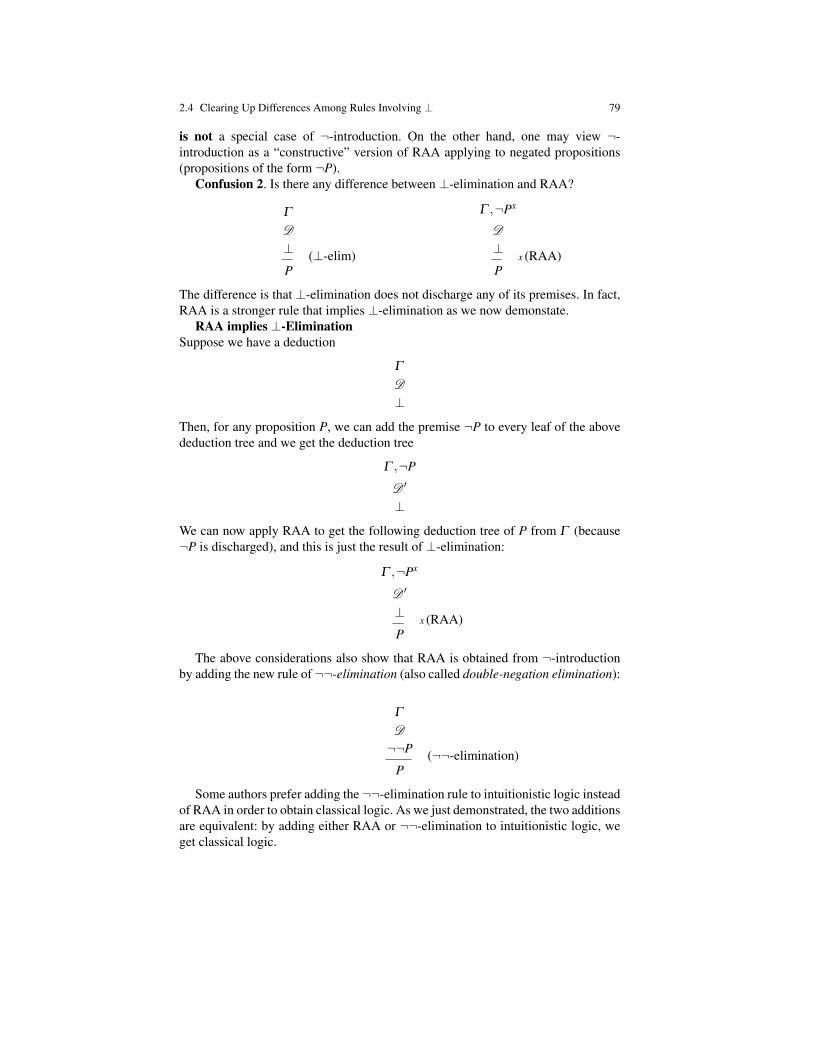
2.4 Clearing Up Differences Among Rules Involving ⊥ 79
is not a special case of ¬-introduction. On the other hand, one may view ¬-introduction as a “constructive” version of RAA applying to negated propositions(propositions of the form ¬P).
Confusion 2. Is there any difference between ⊥-elimination and RAA?
Γ
D
⊥ (⊥-elim)P
Γ ,¬Px
D
⊥x (RAA)
P
The difference is that ⊥-elimination does not discharge any of its premises. In fact,RAA is a stronger rule that implies ⊥-elimination as we now demonstate.
RAA implies ⊥-EliminationSuppose we have a deduction
Γ
D
⊥Then, for any proposition P, we can add the premise ¬P to every leaf of the abovededuction tree and we get the deduction tree
Γ ,¬P
D ′
⊥We can now apply RAA to get the following deduction tree of P from Γ (because¬P is discharged), and this is just the result of ⊥-elimination:
Γ ,¬Px
D ′
⊥x (RAA)
P
The above considerations also show that RAA is obtained from ¬-introductionby adding the new rule of ¬¬-elimination (also called double-negation elimination):
Γ
D
¬¬P (¬¬-elimination)P
Some authors prefer adding the ¬¬-elimination rule to intuitionistic logic insteadof RAA in order to obtain classical logic. As we just demonstrated, the two additionsare equivalent: by adding either RAA or ¬¬-elimination to intuitionistic logic, weget classical logic.
80 2 Mathematical Reasoning And Logic, A Deeper View
There is another way to obtain RAA from the rules of intuitionistic logic, thistime, using the propositions of the form P∨¬P. We saw in Proposition 2.1 that allformulae of the form P∨¬P are provable in classical logic (using RAA).
Confusion 3. Are propositions of the form P ∨ ¬P provable in intuitionisticlogic?The answer is no, which may be disturbing to some readers. In fact, it is quite diffi-cult to prove that propositions of the form P∨¬P are not provable in intuitionisticlogic. One method consists in using the fact that intuitionistic proofs can be normal-ized (see Section 2.11 for more on normalization of proofs). Another method usesKripke models (see Section 2.8 and van Dalen [23]).
Part of the difficulty in understanding at some intuitive level why propositionsof the form P∨¬P are not provable in intuitionistic logic is that the notion of truthbased on the truth values true and false is deeply rooted in all of us. In this frameof mind, it seems ridiculous to question the provability of P∨¬P, because its truthvalue is true whether P is assigned the value true or false. Classical two-valuedtruth value semantics is too crude for intuitionistic logic.
Another difficulty is that it is tempting to equate the notion of truth and the notionof provability. Unfortunately, because classical truth values semantics is too crudefor intuitionistic logic, there are propositions that are universally true (i.e., they eval-uate to true for all possible truth assignments of the atomic letters in them) and yetthey are not provable intuitionistically. The propositions P∨¬P and ¬¬P⇒ P aresuch examples.
One of the major motivations for advocating intuitionistic logic is that it yieldsproofs that are more constructive than classical proofs. For example, in classicallogic, when we prove a disjunction P∨Q, we generally can’t conclude that either Por Q is provable, as exemplified by P∨¬P. A more interesting example involving anonconstructive proof of a disjunction is given in Section 2.5. But, in intuitionisticlogic, from a proof of P∨Q, it is possible to extract either a proof of P or a proofof Q (and similarly for existential statements; see Section 2.9). This property is noteasy to prove. It is a consequence of the normal form for intuitionistic proofs (seeSection 2.11).
In brief, besides being a fun intellectual game, intuitionistic logic is only an in-teresting alternative to classical logic if we care about the constructive nature ofour proofs. But then, we are forced to abandon the classical two-valued truth valuessemantics and adopt other semantics such as Kripke semantics. If we do not careabout the constructive nature of our proofs and if we want to stick to two-valuedtruth values semantics, then we should stick to classical logic. Most people do that,so don’t feel bad if you are not comfortable with intuitionistic logic.
One way to gauge how intuitionisic logic differs from classical logic is to askwhat kind of propositions need to be added to intuitionisic logic in order to get clas-sical logic. It turns out that if all the propositions of the form P∨¬P are consideredto be axioms, then RAA follows from some of the rules of intuitionistic logic.
RAA Holds in Intuitionistic Logic + All Axioms P∨¬P.
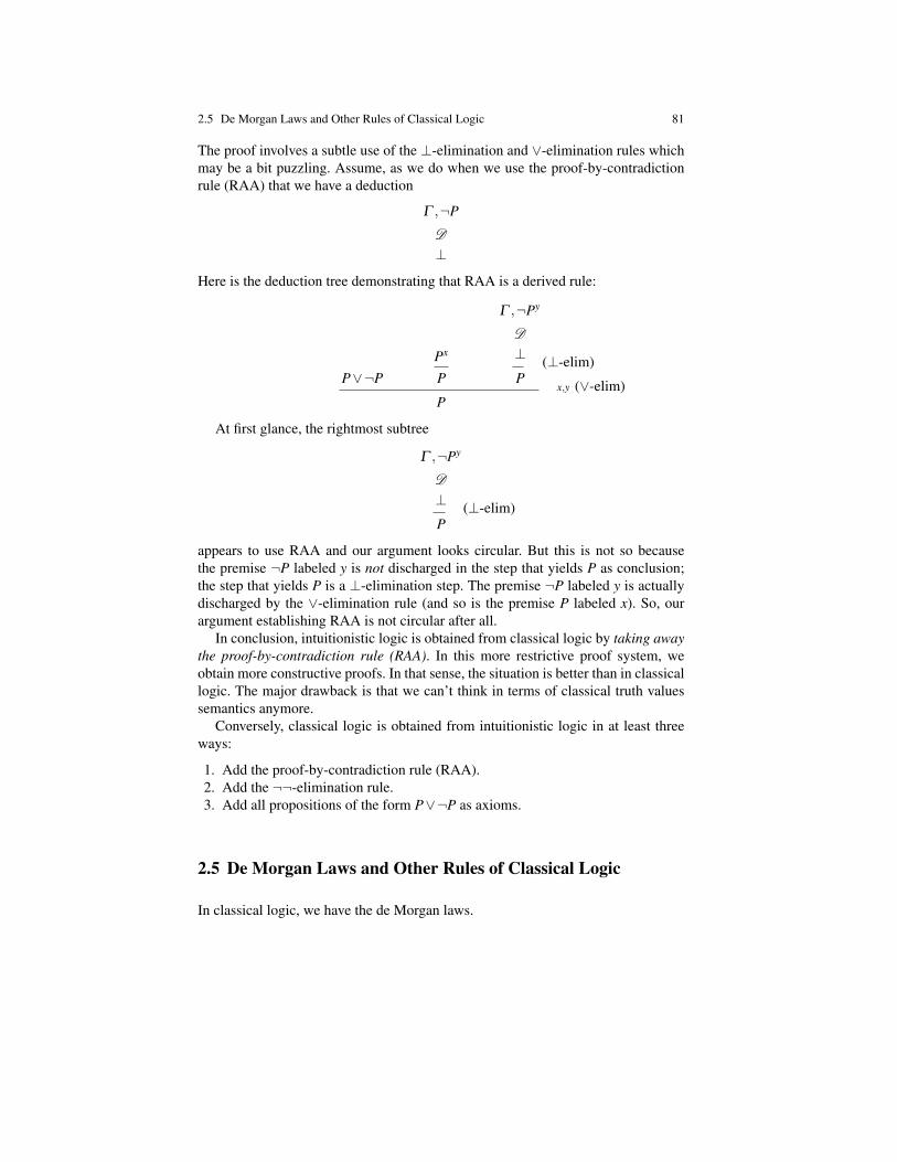
2.5 De Morgan Laws and Other Rules of Classical Logic 81
The proof involves a subtle use of the ⊥-elimination and ∨-elimination rules whichmay be a bit puzzling. Assume, as we do when we use the proof-by-contradictionrule (RAA) that we have a deduction
Γ ,¬P
D
⊥Here is the deduction tree demonstrating that RAA is a derived rule:
P∨¬PPx
P
Γ ,¬Py
D
⊥ (⊥-elim)P
x,y (∨-elim)P
At first glance, the rightmost subtree
Γ ,¬Py
D
⊥ (⊥-elim)P
appears to use RAA and our argument looks circular. But this is not so becausethe premise ¬P labeled y is not discharged in the step that yields P as conclusion;the step that yields P is a ⊥-elimination step. The premise ¬P labeled y is actuallydischarged by the ∨-elimination rule (and so is the premise P labeled x). So, ourargument establishing RAA is not circular after all.
In conclusion, intuitionistic logic is obtained from classical logic by taking awaythe proof-by-contradiction rule (RAA). In this more restrictive proof system, weobtain more constructive proofs. In that sense, the situation is better than in classicallogic. The major drawback is that we can’t think in terms of classical truth valuessemantics anymore.
Conversely, classical logic is obtained from intuitionistic logic in at least threeways:
1. Add the proof-by-contradiction rule (RAA).2. Add the ¬¬-elimination rule.3. Add all propositions of the form P∨¬P as axioms.
2.5 De Morgan Laws and Other Rules of Classical Logic
In classical logic, we have the de Morgan laws.
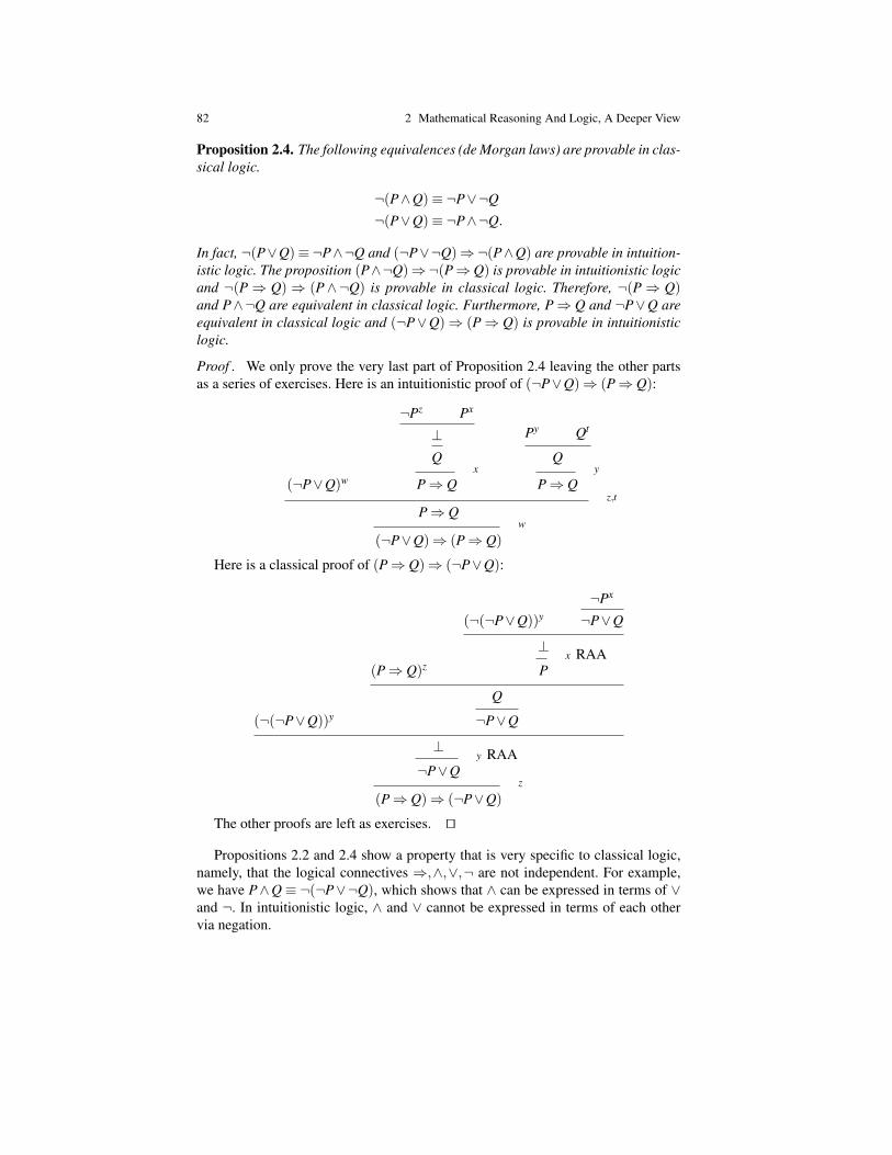
82 2 Mathematical Reasoning And Logic, A Deeper View
Proposition 2.4. The following equivalences (de Morgan laws) are provable in clas-sical logic.
¬(P∧Q)≡ ¬P∨¬Q
¬(P∨Q)≡ ¬P∧¬Q.
In fact, ¬(P∨Q)≡¬P∧¬Q and (¬P∨¬Q)⇒¬(P∧Q) are provable in intuition-istic logic. The proposition (P∧¬Q)⇒¬(P⇒Q) is provable in intuitionistic logicand ¬(P⇒ Q)⇒ (P∧¬Q) is provable in classical logic. Therefore, ¬(P⇒ Q)and P∧¬Q are equivalent in classical logic. Furthermore, P⇒ Q and ¬P∨Q areequivalent in classical logic and (¬P∨Q)⇒ (P⇒ Q) is provable in intuitionisticlogic.
Proof . We only prove the very last part of Proposition 2.4 leaving the other partsas a series of exercises. Here is an intuitionistic proof of (¬P∨Q)⇒ (P⇒ Q):
(¬P∨Q)w
¬Pz Px
⊥Q
x
P⇒ Q
Py Qt
Qy
P⇒ Qz,t
P⇒ Qw
(¬P∨Q)⇒ (P⇒ Q)
Here is a classical proof of (P⇒ Q)⇒ (¬P∨Q):
(¬(¬P∨Q))y
(P⇒ Q)z
(¬(¬P∨Q))y
¬Px
¬P∨Q
⊥x RAA
P
Q
¬P∨Q
⊥y RAA
¬P∨Qz
(P⇒ Q)⇒ (¬P∨Q)
The other proofs are left as exercises. ut
Propositions 2.2 and 2.4 show a property that is very specific to classical logic,namely, that the logical connectives ⇒,∧,∨,¬ are not independent. For example,we have P∧Q ≡ ¬(¬P∨¬Q), which shows that ∧ can be expressed in terms of ∨and ¬. In intuitionistic logic, ∧ and ∨ cannot be expressed in terms of each othervia negation.

2.5 De Morgan Laws and Other Rules of Classical Logic 83
The fact that the logical connectives⇒,∧,∨,¬ are not independent in classicallogic suggests the following question. Are there propositions, written in terms of⇒only, that are provable classically but not provable intuitionistically?
The answer is yes. For instance, the proposition ((P⇒ Q)⇒ P)⇒ P (known asPeirce’s law) is provable classically (do it) but it can be shown that it is not provableintuitionistically.
In addition to the proof-by-cases method and the proof-by-contradiction method,we also have the proof-by-contrapositive method valid in classical logic:
Proof-by-contrapositive rule:
Γ ,¬Qx
D
¬Px
P⇒ Q
This rule says that in order to prove an implication P⇒ Q (from Γ ), one mayassume ¬Q as proved, and then deduce that ¬P is provable from Γ and ¬Q. Thisinference rule is valid in classical logic because we can construct the followingdeduction.
Γ ,¬Qx
D
¬P Py
⊥x (by-contra)
Qy
P⇒ QThe next proposition collects a list of equivalences involving conjunction and dis-
junction that are used all the time. Proofs of these propositions are left as exercises(see the problems).
Proposition 2.5. All the propositions below are provable intuitionistically:
P∨P≡ P
P∧P≡ P
P∨Q≡ Q∨P
P∧Q≡ Q∧P.
The last two assert the commutativity of ∨ and ∧. We have distributivity of ∧ over ∨and of ∨ over ∧:
P∧ (Q∨R)≡ (P∧Q)∨ (P∧R)
P∨ (Q∧R)≡ (P∨Q)∧ (P∨R).
We have associativity of ∧ and ∨:

84 2 Mathematical Reasoning And Logic, A Deeper View
P∧ (Q∧R)≡ (P∧Q)∧R
P∨ (Q∨R)≡ (P∨Q)∨R.
2.6 Formal Versus Informal Proofs; Some Examples
In this section, we give some explicit examples of proofs illustrating the proof prin-ciples that we just discussed. But first, it should be said that it is practically impossi-ble to write formal proofs (i.e., proofs written as proof trees using the rules of one ofthe systems presented earlier) of “real” statements that are not “toy propositions.”This is because it would be extremely tedious and time-consuming to write suchproofs and these proofs would be huge and thus very hard to read.
As we said before it is possible in principle to write formalized proofs, however,most of us will never do so. So, what do we do?
Well, we construct “informal” proofs in which we still make use of the logicalrules that we have presented but we take shortcuts and sometimes we even omitproof steps (some elimination rules, such as ∧-elimination and some introductionrules, such as ∨-introduction) and we use a natural language (here, presumably,English) rather than formal symbols (we say “and” for ∧, “or” for ∨, etc.). As anexample of a shortcut, when using the ∨-elimination rule, in most cases, the disjunc-tion P∨Q has an “obvious proof” because P and Q “exhaust all the cases,” in thesense that Q subsumes ¬P (or P subsumes ¬Q) and classically, P∨¬P is an axiom.Also, we implicitly keep track of the open premises of a proof in our head ratherthan explicitly discharge premises when required. This may be the biggest sourceof mistakes and we should make sure that when we have finished a proof, there areno “dangling premises,” that is, premises that were never used in constructing theproof. If we are “lucky,” some of these premises are in fact unnecessary and weshould discard them. Otherwise, this indicates that there is something wrong withour proof and we should make sure that every premise is indeed used somewhere inthe proof or else look for a counterexample.
We urge our readers to read Chapter 3 of Gowers [10] which contains very illu-minating remarks about the notion of proof in mathematics.
The next question is then, “How does one write good informal proofs?”It is very hard to answer such a question because the notion of a “good” proof is
quite subjective and partly a social concept. Nevertheless, people have been writinginformal proofs for centuries so there are at least many examples of what to do(and what not to do). As with everything else, practicing a sport, playing a musicinstrument, knowing “good” wines, and so on, the more you practice, the better youbecome. Knowing the theory of swimming is fine but you have to get wet and dosome actual swimming. Similarly, knowing the proof rules is important but you haveto put them to use.
Write proofs as much as you can. Find good proof writers (like good swimmers,good tennis players, etc.), try to figure out why they write clear and easily readable
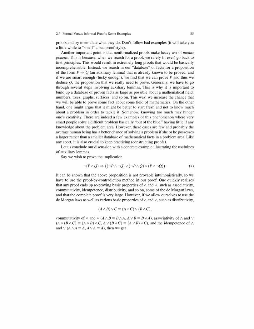
2.6 Formal Versus Informal Proofs; Some Examples 85
proofs and try to emulate what they do. Don’t follow bad examples (it will take youa little while to “smell” a bad proof style).
Another important point is that nonformalized proofs make heavy use of modusponens. This is because, when we search for a proof, we rarely (if ever) go back tofirst principles. This would result in extremely long proofs that would be basicallyincomprehensible. Instead, we search in our “database” of facts for a propositionof the form P⇒ Q (an auxiliary lemma) that is already known to be proved, andif we are smart enough (lucky enough), we find that we can prove P and thus wededuce Q, the proposition that we really need to prove. Generally, we have to gothrough several steps involving auxiliary lemmas. This is why it is important tobuild up a database of proven facts as large as possible about a mathematical field:numbers, trees, graphs, surfaces, and so on. This way, we increase the chance thatwe will be able to prove some fact about some field of mathematics. On the otherhand, one might argue that it might be better to start fresh and not to know muchabout a problem in order to tackle it. Somehow, knowing too much may hinderone’s creativity. There are indeed a few examples of this phenomenon where verysmart people solve a difficult problem basically “out of the blue,” having little if anyknowledge about the problem area. However, these cases are few and probably theaverage human being has a better chance of solving a problem if she or he possessesa larger rather than a smaller database of mathematical facts in a problem area. Likeany sport, it is also crucial to keep practicing (constructing proofs).
Let us conclude our discussion with a concrete example illustrating the usefulnesof auxiliary lemmas.
Say we wish to prove the implication
¬(P∧Q)⇒((¬P∧¬Q)∨ (¬P∧Q)∨ (P∧¬Q)
). (∗)
It can be shown that the above proposition is not provable intuitionistically, so wehave to use the proof-by-contradiction method in our proof. One quickly realizesthat any proof ends up re-proving basic properties of ∧ and ∨, such as associativity,commutativity, idempotence, distributivity, and so on, some of the de Morgan laws,and that the complete proof is very large. However, if we allow ourselves to use thede Morgan laws as well as various basic properties of ∧ and ∨, such as distributivity,
(A∧B)∨C ≡ (A∧C)∨ (B∧C),
commutativity of ∧ and ∨ (A∧B≡ B∧A, A∨B≡ B∨A), associativity of ∧ and ∨(A∧ (B∧C) ≡ (A∧B)∧C, A∨ (B∨C) ≡ (A∨B)∨C), and the idempotence of ∧and ∨ (A∧A≡ A, A∨A≡ A), then we get

86 2 Mathematical Reasoning And Logic, A Deeper View
(¬P∧¬Q)∨ (¬P∧Q)∨ (P∧¬Q) ≡ (¬P∧¬Q)∨ (¬P∧¬Q)
∨ (¬P∧Q)∨ (P∧¬Q)
≡ (¬P∧¬Q)∨ (¬P∧Q)
∨ (¬P∧¬Q)∨ (P∧¬Q)
≡ (¬P∧ (¬Q∨Q))∨ (¬P∧¬Q)∨ (P∧¬Q)
≡ ¬P∨ (¬P∧¬Q)∨ (P∧¬Q)
≡ ¬P∨ ((¬P∨P)∧¬Q)
≡ ¬P∨¬Q,
where we make implicit uses of commutativity and associativity, and the fact thatR∧ (P∨¬P)≡ R, and by de Morgan,
¬(P∧Q)≡ ¬P∨¬Q,
using auxiliary lemmas, we end up proving (∗) without too much pain.And now, we return to some explicit examples of informal proofs.Recall that the set of integers is the set
Z= . . . ,−2,−1,0,1,2, . . .
and that the set of natural numbers is the set
N= 0,1,2, . . ..
(Some authors exclude 0 from N. We don’t like this discrimination against zero.) Ainteger a ∈ Z is even if it is of the form a = 2b for some b ∈ Z, odd if it is of theform a = 2b+ 1 for some b ∈ Z. The following facts are essentially obvious fromthe definition of even and odd.
(a) The sum of even integers is even.(b) The sum of an even integer and of an odd integer is odd.(c) The sum of two odd integers is even.(d) The product of odd integers is odd.(e) The product of an even integer with any integer is even.
Now, we prove the following fact using the proof-by-cases method.
Proposition 2.6. Let a,b,c be odd integers. For any integers p and q, if p and q arenot both even, then
ap2 +bpq+ cq2
is odd.
Proof . We consider the three cases:
1. p and q are odd. In this case as a,b, and c are odd, by (d) all the productsap2,bpq, and cq2 are odd. By (c), ap2+bpq is even and by (b), ap2+bpq+cq2
is odd.
2.6 Formal Versus Informal Proofs; Some Examples 87
2. p is even and q is odd. In this case, by (e), both ap2 and bpq are even and by(d), cq2 is odd. But then, by (a), ap2 +bpq is even and by (b), ap2 +bpq+ cq2
is odd.3. p is odd and q is even. This case is analogous to the previous case, except that p
and q are interchanged. The reader should have no trouble filling in the details.
All three cases exhaust all possibilities for p and q not to be both even, thus theproof is complete by the ∨-elimination rule (applied twice). ut
The set of rational numbers Q consists of all fractions p/q, where p,q ∈ Z, withq 6= 0. The set of real numbers is denoted by R. A real number, a ∈ R, is said to beirrational if it cannot be expressed as a number in Q (a fraction).
We now use Proposition 2.6 and the proof by contradiction method to prove thefollowing.
Proposition 2.7. Let a,b,c be odd integers. Then, the equation
aX2 +bX + c = 0
has no rational solution X. Equivalently, every zero of the above equation is irra-tional.
Proof . We proceed by contradiction (by this, we mean that we use the proof-by-contradiction rule). So, assume that there is a rational solution X = p/q. We mayassume that p and q have no common divisor, which implies that p and q are notboth even. As q 6= 0, if aX2 +bX + c = 0, then by multiplying by q2, we get
ap2 +bpq+ cq2 = 0.
However, as p and q are not both even and a,b,c are odd, we know from Proposition2.6 that ap2 + bpq+ cq2 is odd. This contradicts the fact that p2 + bpq+ cq2 = 0and thus, finishes the proof. ut
Remark: A closer look at the proof of Proposition 2.7 shows that rather than us-ing the proof-by-contradiction rule we really used ¬-introduction (a “constructive”version of RAA).
As as example of the proof-by-contrapositive method, we prove that if an integern2 is even, then n must be even.
Observe that if an integer is not even then it is odd (and vice versa). This factmay seem quite obvious but to prove it actually requires using induction (which wehaven’t officially met yet). A rigorous proof is given in Section 2.10.
Now, the contrapositive of our statement is: if n is odd, then n2 is odd. But, tosay that n is odd is to say that n = 2k+1 and then, n2 = (2k+1)2 = 4k2 +4k+1 =2(2k2 +2k)+1, which shows that n2 is odd.
As it is, because the above proof uses the proof-by-contrapositive method, it isnot constructive. Thus, the question arises, is there a constructive proof of the abovefact?
88 2 Mathematical Reasoning And Logic, A Deeper View
Indeed there is a constructive proof if we observe that every integer n is eithereven or odd but not both. Now, one might object that we just relied on the law of theexcluded middle but there is a way to circumvent this problem by using induction;see Section 2.10 for a rigorous proof.
Now, because an integer is odd iff it is not even, we may proceed to prove thatif n2 is even, then n is not odd, by using our constructive version of the proof-by-contradiction principle, namely, ¬-introduction.
Therefore, assume that n2 is even and that n is odd. Then, n = 2k + 1, whichimplies that n2 = 4k2 +4k+1 = 2(2k2 +2k)+1, an odd number, contradicting thefact that n2 is assumed to be even. ut
As another illustration of the proof methods that we have just presented, let usprove that
√2 is irrational, which means that
√2 is not rational. The reader may also
want to look at the proof given by Gowers in Chapter 3 of his book [10]. Obviously,our proof is similar but we emphasize step (2) a little more.
Because we are trying to prove that√
2 is not rational, let us use our constructiveversion of the proof-by-contradiction principle, namely, ¬-introduction. Thus, letus assume that
√2 is rational and derive a contradiction. Here are the steps of the
proof.
1. If√
2 is rational, then there exist some integers p,q ∈ Z, with q 6= 0, so that√2 = p/q.
2. Any fraction p/q is equal to some fraction r/s, where r and s are not both even.3. By (2), we may assume that √
2 =pq,
where p,q ∈ Z are not both even and with q 6= 0.4. By (3), because q 6= 0, by multiplying both sides by q, we get
q√
2 = p.
5. By (4), by squaring both sides, we get
2q2 = p2.
6. Inasmuch as p2 = 2q2, the number p2 must be even. By a fact previously estab-lished, p itself is even; that is, p = 2s, for some s ∈ Z.
7. By (6), if we substitute 2s for p in the equation in (5) we get 2q2 = 4s2. Bydividing both sides by 2, we get
q2 = 2s2.
8. By (7), we see that q2 is even, from which we deduce (as above) that q itself iseven.
9. Now, assuming that√
2 = p/q where p and q are not both even (and q 6= 0),we concluded that both p and q are even (as shown in (6) and(8)), reaching

2.6 Formal Versus Informal Proofs; Some Examples 89
a contradiction. Therefore, by negation introduction, we proved that√
2 is notrational.
A closer examination of the steps of the above proof reveals that the only stepthat may require further justification is step (2): that any fraction p/q is equal tosome fraction r/s where r and s are not both even.
This fact does require a proof and the proof uses the division algorithm, whichitself requires induction (see Section 7.3, Theorem 7.7). Besides this point, all theother steps only require simple arithmetic properties of the integers and are con-structive.
Remark: Actually, every fraction p/q is equal to some fraction r/s where r and shave no common divisor except 1. This follows from the fact that every pair of inte-gers has a greatest common divisor (a gcd; see Section 7.4) and r and s are obtainedby dividing p and q by their gcd. Using this fact and Euclid’s lemma (Proposition7.9), we can obtain a shorter proof of the irrationality of
√2. First, we may assume
that p and q have no common divisor besides 1 (we say that p and q are relativelyprime). From (5), we have
2q2 = p2,
so q divides p2. However, q and p are relatively prime and as q divides p2 = p× p,by Euclid’s lemma, q divides p. But because 1 is the only common divisor of p andq, we must have q = 1. Now, we get p2 = 2, which is impossible inasmuch as 2 isnot a perfect square.
The above argument can be easily adapted to prove that if the positive integer nis not a perfect square, then
√n is not rational.
Let us return briefly to the issue of constructivity in classical logic, in particularwhen it comes to disjunctions.
Consider the question: are there two irrational real numbers a and b such that ab
is rational? Here is a way to prove that this is indeed the case. Consider the number√
2√
2. If this number is rational, then a =
√2 and b =
√2 is an answer to our
question (because we already know that√
2 is irrational). Now, observe that
(√
2√
2)√
2 =√
2√
2×√
2=√
22= 2 is rational.
Thus, if√
2√
2is irrational, then a =
√2√
2and b =
√2 is an answer to our question.
Because P∨¬P is provable (the law of the excluded middle;√
2√
2is rational or it
is not rational), we proved that
(√
2 is irrational and√
2√
2is rational) or
(√
2√
2and√
2 are irrational and (√
2√
2)√
2 is rational).
However, the above proof does not tell us whether√
2√
2is rational!
We see one of the shortcomings of classical reasoning: certain statements (inparticular, disjunctive or existential) are provable but their proof does not providean explicit answer. It is in that sense that classical logic is not constructive.
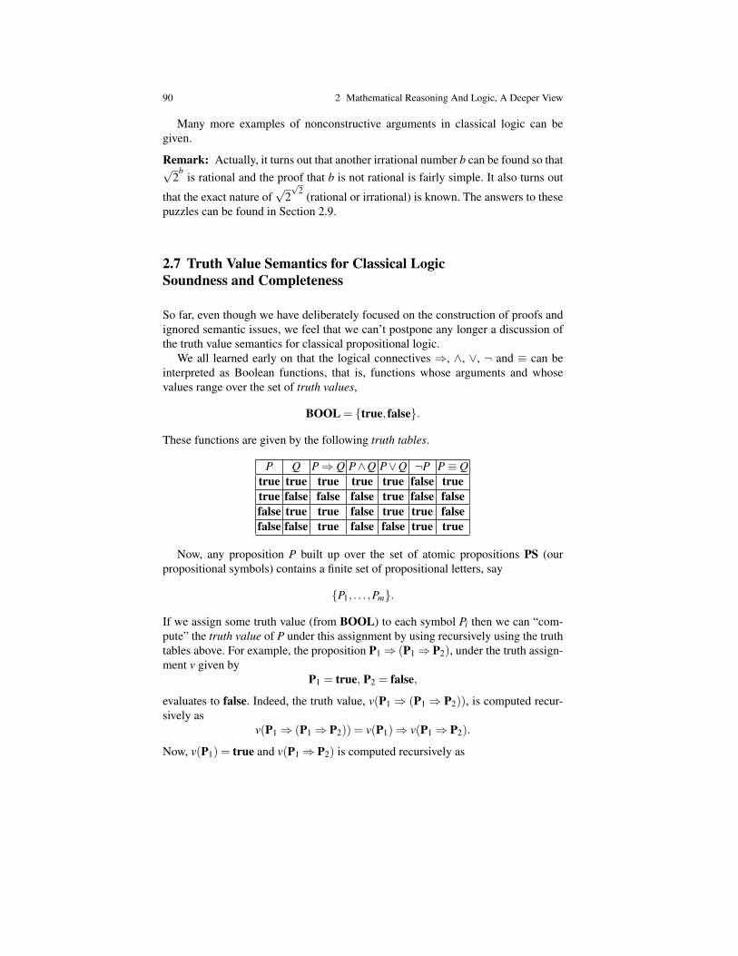
90 2 Mathematical Reasoning And Logic, A Deeper View
Many more examples of nonconstructive arguments in classical logic can begiven.
Remark: Actually, it turns out that another irrational number b can be found so that√2
bis rational and the proof that b is not rational is fairly simple. It also turns out
that the exact nature of√
2√
2(rational or irrational) is known. The answers to these
puzzles can be found in Section 2.9.
2.7 Truth Value Semantics for Classical LogicSoundness and Completeness
So far, even though we have deliberately focused on the construction of proofs andignored semantic issues, we feel that we can’t postpone any longer a discussion ofthe truth value semantics for classical propositional logic.
We all learned early on that the logical connectives ⇒, ∧, ∨, ¬ and ≡ can beinterpreted as Boolean functions, that is, functions whose arguments and whosevalues range over the set of truth values,
BOOL = true, false.
These functions are given by the following truth tables.
P Q P⇒ Q P∧Q P∨Q ¬P P≡ Qtrue true true true true false truetrue false false false true false falsefalse true true false true true falsefalse false true false false true true
Now, any proposition P built up over the set of atomic propositions PS (ourpropositional symbols) contains a finite set of propositional letters, say
P1, . . . ,Pm.
If we assign some truth value (from BOOL) to each symbol Pi then we can “com-pute” the truth value of P under this assignment by using recursively using the truthtables above. For example, the proposition P1⇒ (P1⇒ P2), under the truth assign-ment v given by
P1 = true, P2 = false,
evaluates to false. Indeed, the truth value, v(P1⇒ (P1⇒ P2)), is computed recur-sively as
v(P1⇒ (P1⇒ P2)) = v(P1)⇒ v(P1⇒ P2).
Now, v(P1) = true and v(P1⇒ P2) is computed recursively as

2.7 Truth Value Semantics for Classical Logic 91
v(P1⇒ P2) = v(P1)⇒ v(P2).
Because v(P1) = true and v(P2) = false, using our truth table, we get
v(P1⇒ P2) = true⇒ false = false.
Plugging this into the right-hand side of v(P1⇒ (P1⇒ P2)), we finally get
v(P1⇒ (P1⇒ P2)) = true⇒ false = false.
However, under the truth assignment v given by
P1 = true, P2 = true,
we find that our proposition evaluates to true.The values of a proposition can be determined by creating a truth table, in which
a proposition is evaluated by computing recursively the truth values of its subexpres-sions. For example, the truth table corresponding to the proposition P1⇒ (P1⇒P2)is
P1 P2 P1⇒ P2 P1⇒ (P1⇒ P2)
true true true truetrue false false falsefalse true true truefalse false true true
If we now consider the proposition P = (P1⇒ (P2⇒ P1)), its truth table is
P1 P2 P2⇒ P1 P1⇒ (P2⇒ P1)
true true true truetrue false true truefalse true false truefalse false true true
which shows that P evaluates to true for all possible truth assignments.The truth table of a proposition containing m variables has 2m rows. When m is
large, 2m is very large, and computing the truth table of a proposition P may not bepractically feasible. Even the problem of finding whether there is a truth assignmentthat makes P true is hard.
Definition 2.5. We say that a proposition P is satisfiable iff it evaluates to true forsome truth assignment (taking values in BOOL) of the propositional symbols oc-curring in P and otherwise we say that it is unsatisfiable. A proposition P is valid(or a tautology) iff it evaluates to true for all truth assignments of the propositionalsymbols occurring in P.
92 2 Mathematical Reasoning And Logic, A Deeper View
Observe that a proposition P is valid if in the truth table for P all the entries inthe column corresponding to P have the value true. The proposition P is satisfiableif some entry in the column corresponding to P has the value true.
The problem of deciding whether a proposition is satisfiable is called the satisfia-bility problem and is sometimes denoted by SAT. The problem of deciding whethera proposition is valid is called the validity problem.
For example, the proposition
P = (P1∨¬P2∨¬P3)∧ (¬P1∨¬P3)∧ (P1∨P2∨P4)∧ (¬P3∨P4)∧ (¬P1∨P4)
is satisfiable because it evaluates to true under the truth assignment P1 = true,P2 = false, P3 = false, and P4 = true. On the other hand, the proposition
Q = (P1∨P2∨P3)∧ (¬P1∨P2)∧ (¬P2∨P3)∧ (P1∨¬P3)∧ (¬P1∨¬P2∨¬P3)
is unsatisfiable as one can verify by trying all eight truth assignments for P1, P2, P3.The reader should also verify that the proposition
R = (¬P1∧¬P2∧¬P3)∨ (P1∧¬P2)∨ (P2∧¬P3)∨ (¬P1∧P3)∨ (P1∧P2∧P3)
is valid (observe that the proposition R is the negation of the proposition Q).The satisfiability problem is a famous problem in computer science because of
its complexity. Try it; solving it is not as easy as you think. The difficulty is that ifa proposition P contains n distinct propositional letters, then there are 2n possibletruth assignments and checking all of them is practically impossible when n is large.
In fact, the satisfiability problem turns out to be an NP-complete problem, a veryimportant concept that you will learn about in a course on the theory of compu-tation and complexity. Very good expositions of this kind of material are found inHopcroft, Motwani, and Ullman [12] and Lewis and Papadimitriou [16]. The valid-ity problem is also important and it is related to SAT. Indeed, it is easy to see that aproposition P is valid iff ¬P is unsatisfiable.
What’s the relationship between validity and provability in the system N ⇒,∧,∨,⊥c
(or N G⇒,∧,∨,⊥c )?
Remarkably, in classical logic, validity and provability are equivalent.In order to prove the above claim, we need to do two things:
(1) Prove that if a proposition P is provable in the system N ⇒,∧,∨,⊥c (or the system
N G⇒,∧,∨,⊥c ), then it is valid. This is known as soundness or consistency (of the
proof system).(2) Prove that if a proposition P is valid, then it has a proof in the system N ⇒,∧,∨,⊥
c(or N G⇒,∧,∨,⊥
c ). This is known as the completeness (of the proof system).
In general, it is relatively easy to prove (1) but proving (2) can be quite com-plicated. In fact, some proof systems are not complete with respect to certainsemantics. For instance, the proof system for intuitionistic logic N ⇒,∧,∨,⊥
i (orN G⇒,∧,∨,⊥
i ) is not complete with respect to truth value semantics. As an exam-

2.7 Truth Value Semantics for Classical Logic 93
ple, ((P⇒ Q)⇒ P)⇒ P (known as Peirce’s law), is valid but it can be shown thatit cannot be proved in intuitionistic logic.
In this book, we content ourselves with soundness.
Proposition 2.8. (Soundness of N ⇒,∧,∨,⊥c and N G⇒,∧,∨,⊥
c ) If a proposition P isprovable in the system N ⇒,∧,∨,⊥
c (or N G⇒,∧,∨,⊥c ), then it is valid (according to the
truth value semantics).
Sketch of Proof . It is enough to prove that if there is a deduction of a proposition Pfrom a set of premises Γ then for every truth assignment for which all the proposi-tions in Γ evaluate to true, then P evaluates to true. However, this is clear for theaxioms and every inference rule preserves that property.
Now, if P is provable, a proof of P has an empty set of premises and so P evaluatesto true for all truth assignments, which means that P is valid. ut
Theorem 2.1. (Completeness of N ⇒,∧,∨,⊥c and N G⇒,∧,∨,⊥
c ) If a proposition P isvalid (according to the truth value semantics), then P is provable in the systemN ⇒,∧,∨,⊥
c (or N G⇒,∧,∨,⊥c ).
Proofs of completeness for classical logic can be found in van Dalen [23] orGallier [4] (but for a different proof system).
Soundness (Proposition 2.8) has a very useful consequence: in order to provethat a proposition P is not provable, it is enough to find a truth assignment for whichP evaluates to false. We say that such a truth assignment is a counterexample forP (or that P can be falsified). For example, no propositional symbol Pi is provablebecause it is falsified by the truth assignment Pi = false.
The soundness of the proof system N ⇒,∧,∨,⊥c (or N G⇒,∧,∨,⊥
c ) also has the ex-tremely important consequence that⊥ cannot be proved in this system, which meansthat contradictory statements cannot be derived.
This is by no means obvious at first sight, but reassuring. It is also possible toprove that the proof system N ⇒,∧,∨,⊥
c is consistent (i.e., ⊥ cannot be proved) bypurely proof-theoretic means involving proof normalization (See Section 2.11), butthis requires a lot more work.
Note that completeness amounts to the fact that every unprovable formula has acounterexample. Also, in order to show that a proposition is classically provable, itsuffices to compute its truth table and check that the proposition is valid. This maystill be a lot of work, but it is a more “mechanical” process than attempting to find aproof.
For example, here is a truth table showing that (P1⇒ P2)≡ (¬P1∨P2) is valid.
P1 P2 P1⇒ P2 ¬P1∨P2 (P1⇒ P2)≡ (¬P1∨P2)true true true true truetrue false false false truefalse true true true truefalse false true true true
94 2 Mathematical Reasoning And Logic, A Deeper View
Remark: Truth value semantics is not the right kind of semantics for intuitionisticlogic; it is too coarse. A more subtle kind of semantics is required. Among thevarious semantics for intuitionistic logic, one of the most natural is the notion ofthe Kripke model. Then, again, soundness and completeness hold for intuitionisticproof systems (see Section 2.8 and van Dalen [23]).
Fig. 2.3 Saul Kripke, 1940–
2.8 Kripke Models for Intuitionistic LogicSoundness and Completeness
In this section, we briefly describe the semantics of intuitionistic propositional logicin terms of Kripke models. This section has been included to quench the thirst ofthose readers who can’t wait to see what kind of decent semantics can be givenfor intuitionistic propositional logic and it can be safely omitted. We recommendreviewing the material of Section 7.1 before reading this section.
In classical truth value semantics based on BOOL = true, false, we might saythat truth is absolute. The idea of Kripke semantics is that there is a set of worlds Wtogether with a partial ordering ≤ on W , and that truth depends on in which worldwe are. Furthermore, as we “go up” from a world u to a world v with u ≤ v, truth“can only increase,” that is, whatever is true in world u remains true in world v. Also,the truth of some propositions, such as P⇒ Q or ¬P, depends on “future worlds.”With this type of semantics, which is no longer absolute, we can capture exactly theessence of intuitionistic logic. We now make these ideas precise.
Definition 2.6. A Kripke model for intuitionistic propositional logic is a pair K =(W,ϕ) where W is a partially ordered (nonempty) set called a set of worlds and ϕ isa function ϕ : W → BOOLPS such that for every u ∈W , the function ϕ(u) : PS→BOOL is an assignment of truth values to the propositional symbols in PS satisfyingthe following property. For all u,v ∈W , for all Pi ∈ PS,
if u≤ v and ϕ(u)(Pi) = true, then ϕ(v)(Pi) = true.
2.8 Kripke Models for Intuitionistic Logic 95
As we said in our informal comments, truth can’t decrease when we move from aworld u to a world v with u≤ v but truth can increase; it is possible that ϕ(u)(Pi) =false and yet, ϕ(v)(Pi) = true. We use Kripke models to define the semantics ofpropositions as follows.
Definition 2.7. Given a Kripke model K = (W,ϕ), for every u ∈W and for everyproposition P we say that P is satisfied by K at u and we write ϕ(u)(P) = true iff
(a) ϕ(u)(Pi) = true, if P = Pi ∈ PS.(b) ϕ(u)(Q) = true and ϕ(u)(R) = true, if P = Q∧R.(c) ϕ(u)(Q) = true or ϕ(u)(R) = true, if P = Q∨R.(d) For all v such that u≤ v, if ϕ(v)(Q) = true, then ϕ(v)(R) = true, if P = Q⇒ R.(e) For all v such that u≤ v, ϕ(v)(Q) = false, if P = ¬Q.(f) ϕ(u)(⊥) = false; that is, ⊥ is not satisfied by K at u (for any K and any u).
We say that P is valid in K (or that K is a model of P) iff P is satisfied by K =(W,ϕ) at u for all u ∈W and we say that P is intuitionistically valid iff P is valid inevery Kripke model K .
When P is satisfied by K at u we also say that P is true at u in K . Note that thetruth at u ∈W of a proposition of the form Q⇒ R or ¬Q depends on the truth of Qand R at all “future worlds,” v ∈W , with u ≤ v. Observe that classical truth valuesemantics corresponds to the special case where W consists of a single element (asingle world).
If W = 0,1 ordered so that 0≤ 1 and if ϕ is given by
ϕ(0)(Pi) = falseϕ(1)(Pi) = true,
then Kbad = (W,ϕ) is a Kripke structure. The reader should check that the proposi-tion P = (Pi∨¬Pi) has the value false at 0 because ϕ(0)(Pi) = false but ϕ(1)(Pi) =true, so clause (e) fails for ¬Pi at u = 0. Therefore, P = (Pi ∨¬Pi) is not valid inKbad and thus, it is not intuitionistically valid. We escaped the classical truth valuesemantics by using a universe with two worlds. The reader should also check that
ϕ(u)(¬¬P) = true iff for all v such that u≤ v
there is some w with v≤ w so that ϕ(w)(P) = true.
This shows that in Kripke semantics, ¬¬P is weaker than P, in the sense thatϕ(u)(¬¬P) = true does not necessarily imply that ϕ(u)(P) = true. The readershould also check that the proposition ¬¬Pi⇒ Pi is not valid in the Kripke structureKbad.
As we said in the previous section, Kripke semantics is a perfect fit to intuition-istic provability in the sense that soundness and completeness hold.
Proposition 2.9. (Soundness of N ⇒,∧,∨,⊥i and N G⇒,∧,∨,⊥
i ) If a proposition P isprovable in the system N ⇒,∧,∨,⊥
i (or N G⇒,∧,∨,⊥i ), then it is valid in every Kripke
model, that is, it is intuitionistically valid.
96 2 Mathematical Reasoning And Logic, A Deeper View
Proposition 2.9 is not hard to prove. We consider any deduction of a propositionP from a set of premises Γ and we prove that for every Kripke model K = (W,ϕ),for every u ∈W , if every premise in Γ is satisfied by K at u, then P is also satisfiedby K at u. This is obvious for the axioms and it is easy to see that the inferencerules preserve this property.
Completeness also holds, but it is harder to prove (see van Dalen [23]).
Theorem 2.2. (Completeness of N ⇒,∧,∨,⊥i and N G⇒,∧,∨,⊥
i ) If a proposition P isintuitionistically valid, then P is provable in the system N ⇒,∧,∨,⊥
i (or N G⇒,∧,∨,⊥i ).
Another proof of completeness for a different proof system for propositional in-tuitionistic logic (a Gentzen-sequent calculus equivalent to N G⇒,∧,∨,⊥
i ) is given inTakeuti [21]. We find this proof more instructive than van Dalen’s proof. This proofalso shows that if a proposition P is not intuitionistically provable, then there is aKripke model K where W is a finite tree in which P is not valid. Such a Kripkemodel is called a counterexample for P.
We now add quantifiers to our language and give the corresponding inferencerules.
2.9 Adding Quantifiers; The Proof Systems N ⇒,∧,∨,∀,∃,⊥c ,
N G⇒,∧,∨,∀,∃,⊥c
As we mentioned in Section 2.1, atomic propositions may contain variables. Theintention is that such variables correspond to arbitrary objects. An example is
human(x)⇒ needs-to-drink(x).
Now, in mathematics, we usually prove universal statements, that is statements thathold for all possible “objects,” or existential statements, that is, statements assertingthe existence of some object satisfying a given property. As we saw earlier, we assertthat every human needs to drink by writing the proposition
∀x(human(x)⇒ needs-to-drink(x)).
Observe that once the quantifier ∀ (pronounced “for all” or “for every”) is appliedto the variable x, the variable x becomes a placeholder and replacing x by y or anyother variable does not change anything. What matters is the locations to which theouter x points in the inner proposition. We say that x is a bound variable (sometimesa “dummy variable”).
If we want to assert that some human needs to drink we write
∃x(human(x)⇒ needs-to-drink(x));
Again, once the quantifier ∃ (pronounced “there exists”) is applied to the variable x,the variable x becomes a placeholder. However, the intended meaning of the second
2.9 Adding Quantifiers; The Proof Systems N ⇒,∧,∨,∀,∃,⊥c , N G⇒,∧,∨,∀,∃,⊥
c 97
proposition is very different and weaker than the first. It only asserts the existenceof some object satisfying the statement
human(x)⇒ needs-to-drink(x).
Statements may contain variables that are not bound by quantifiers. For example,in
∃x parent(x,y)
the variable x is bound but the variable y is not. Here, the intended meaning ofparent(x,y) is that x is a parent of y, and the intended meaning of ∃x parent(x,y) isthat any given y has some parent x. Variables that are not bound are called free. Theproposition
∀y∃x parent(x,y),
which contains only bound variables is meant to assert that every y has some par-ent x. Typically, in mathematics, we only prove statements without free variables.However, statements with free variables may occur during intermediate stages of aproof.
The intuitive meaning of the statement ∀xP is that P holds for all possible objectsx and the intuitive meaning of the statement ∃xP is that P holds for some object x.Thus, we see that it would be useful to use symbols to denote various objects. Forexample, if we want to assert some facts about the “parent” predicate, we may wantto introduce some constant symbols (for short, constants) such as “Jean,” “Mia,” andso on and write
parent(Jean,Mia)
to assert that Jean is a parent of Mia. Often, we also have to use function symbols(or operators, constructors), for instance, to write a statement about numbers: +, ∗,and so on. Using constant symbols, function symbols, and variables, we can formterms, such as
(x∗ x+1)∗ (3∗ y+2).
In addition to function symbols, we also use predicate symbols, which are namesfor atomic properties. We have already seen several examples of predicate symbols:“human,” “parent.” So, in general, when we try to prove properties of certain classesof objects (people, numbers, strings, graphs, and so on), we assume that we have acertain alphabet consisting of constant symbols, function symbols, and predicatesymbols. Using these symbols and an infinite supply of variables (assumed distinctfrom the variables we use to label premises) we can form terms and predicate terms.We say that we have a (logical) language. Using this language, we can write com-pound statements.
Let us be a little more precise. In a first-order language L in addition to thelogical connectives⇒,∧,∨,¬,⊥, ∀, and ∃, we have a set L of nonlogical symbolsconsisting of
(i) A set CS of constant symbols, c1,c2, . . . ,.

98 2 Mathematical Reasoning And Logic, A Deeper View
(ii) A set FS of function symbols, f1, f2, . . . ,. Each function symbol f has a rankn f ≥ 1, which is the number of arguments of f .
(iii) A set PS of predicate symbols, P1,P2, . . . ,. Each predicate symbol P has a ranknP ≥ 0, which is the number of arguments of P. Predicate symbols of rank 0are propositional symbols as in earlier sections.
(iv) The equality predicate = is added to our language when we want to deal withequations.
(v) First-order variables t1, t2, . . . used to form quantified formulae.
The difference between function symbols and predicate symbols is that functionsymbols are interpreted as functions defined on a structure (e.g., addition, +, onN), whereas predicate symbols are interpreted as properties of objects, that is, theytake the value true or false. An example is the language of Peano arithmetic, L =0,S,+,∗,=. Here, the intended structure is N, 0 is of course zero, S is interpretedas the function S(n) = n+1, the symbol + is addition, ∗ is multiplication, and = isequality.
Using a first-order language L, we can form terms, predicate terms, and formulae.The terms over L are the following expressions.
(i) Every variable t is a term.(ii) Every constant symbol c ∈ CS, is a term.
(iii) If f ∈ FS is a function symbol taking n arguments and τ1, . . . ,τn are termsalready constructed, then f (τ1, . . . ,τn) is a term.
The predicate terms over L are the following expressions.
(i) If P ∈ PS is a predicate symbol taking n arguments and τ1, . . . ,τn are termsalready constructed, then P(τ1, . . . ,τn) is a predicate term. When n = 0, thepredicate symbol P is a predicate term called a propositional symbol.
(ii) When we allow the equality predicate, for any two terms τ1 and τ2, the expres-sion τ1 = τ2 is a predicate term. It is usually called an equation.
The (first-order) formulae over L are the following expressions.
(i) Every predicate term P(τ1, . . . ,τn) is an atomic formula. This includes allpropositional letters. We also view⊥ (and sometimes>) as an atomic formula.
(ii) When we allow the equality predicate, every equation τ1 = τ2 is an atomicformula.
(iii) If P and Q are formulae already constructed, then P⇒Q, P∧Q, P∨Q, ¬P arecompound formulae. We treat P≡Q as an abbreviation for (P⇒Q)∧(Q⇒P),as before.
(iv) If P is a formula already constructed and t is any variable, then ∀tP and ∃tPare quantified compound formulae.
All this can be made very precise but this is quite tedious. Our primary goal isto explain the basic rules of logic and not to teach a full-fledged logic course. Wehope that our intuitive explanations will suffice and we now come to the heart of the
2.9 Adding Quantifiers; The Proof Systems N ⇒,∧,∨,∀,∃,⊥c , N G⇒,∧,∨,∀,∃,⊥
c 99
matter, the inference rules for the quantifiers. Once again, for a complete treatment,readers are referred to Gallier [4], van Dalen [23], or Huth and Ryan [14].
Unlike the rules for ⇒,∨,∧ and ⊥, which are rather straightforward, the rulesfor quantifiers are more subtle due to the presence of variables (occurring in termsand predicates). We have to be careful to forbid inferences that would yield “wrong”results and for this we have to be very precise about the way we use free variables.More specifically, we have to exercise care when we make substitutions of terms forvariables in propositions. For example, say we have the predicate “odd,” intendedto express that a number is odd. Now, we can substitute the term (2y+1)2 for x inodd(x) and obtain
odd((2y+1)2).
More generally, if P(t1, t2, . . . , tn) is a statement containing the free variables t1, . . . , tnand if τ1, . . . ,τn are terms, we can form the new statement
P[τ1/t1, . . . ,τn/tn]
obtained by substituting the term τi for all free occurrences of the variable ti, fori = 1, . . . ,n. By the way, we denote terms by the Greek letter τ because we use theletter t for a variable and using t for both variables and terms would be confusing;sorry.
However, if P(t1, t2, . . . , tn) contains quantifiers, some bad things can happen;namely, some of the variables occurring in some term τi may become quantifiedwhen τi is substituted for ti. For example, consider
∀x∃yP(x,y,z)
which contains the free variable z and substitute the term x+ y for z: we get
∀x∃yP(x,y,x+ y).
We see that the variables x and y occurring in the term x+y become bound variablesafter substitution. We say that there is a “capture of variables.”
This is not what we intended to happen. To fix this problem, we recall that boundvariables are really place holders, so they can be renamed without changing any-thing. Therefore, we can rename the bound variables x and y in ∀x∃yP(x,y,z) to uand v, getting the statement ∀u∃vP(u,v,z) and now, the result of the substitution is
∀u∃vP(u,v,x+ y).
Again, all this needs to be explained very carefuly but this can be done.Finally, here are the inference rules for the quantifiers, first stated in a natural
deduction style and then in sequent style. It is assumed that we use two disjointsets of variables for labeling premises (x,y, . . .) and free variables (t,u,v, . . .). As weshow, the ∀-introduction rule and the ∃-elimination rule involve a crucial restrictionon the occurrences of certain variables. Remember, variables are terms.
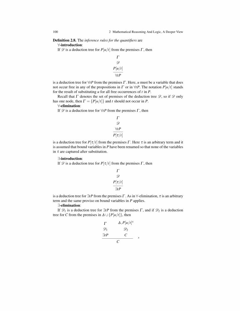
100 2 Mathematical Reasoning And Logic, A Deeper View
Definition 2.8. The inference rules for the quantifiers are∀-introduction:If D is a deduction tree for P[u/t] from the premises Γ , then
Γ
D
P[u/t]
∀tPis a deduction tree for ∀tP from the premises Γ . Here, u must be a variable that doesnot occur free in any of the propositions in Γ or in ∀tP. The notation P[u/t] standsfor the result of substituting u for all free occurrences of t in P.
Recall that Γ denotes the set of premises of the deduction tree D , so if D onlyhas one node, then Γ = P[u/t] and t should not occur in P.∀-elimination:If D is a deduction tree for ∀tP from the premises Γ , then
Γ
D
∀tPP[τ/t]
is a deduction tree for P[τ/t] from the premises Γ . Here τ is an arbitrary term and itis assumed that bound variables in P have been renamed so that none of the variablesin τ are captured after substitution.
∃-introduction:If D is a deduction tree for P[τ/t] from the premises Γ , then
Γ
D
P[τ/t]
∃tPis a deduction tree for ∃tP from the premises Γ . As in ∀-elimination, τ is an arbitraryterm and the same proviso on bound variables in P applies.∃-elimination:If D1 is a deduction tree for ∃tP from the premises Γ , and if D2 is a deduction
tree for C from the premises in ∆ ∪P[u/t], then
Γ
D1
∃tP
∆ ,P[u/t]x
D2
Cx
C
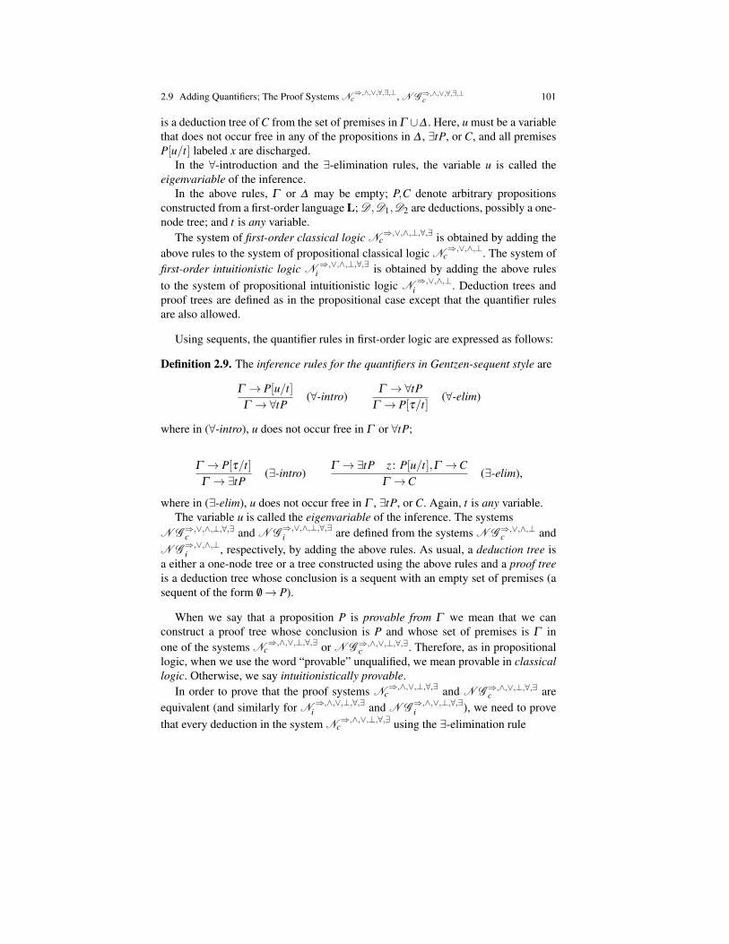
2.9 Adding Quantifiers; The Proof Systems N ⇒,∧,∨,∀,∃,⊥c , N G⇒,∧,∨,∀,∃,⊥
c 101
is a deduction tree of C from the set of premises in Γ ∪∆ . Here, u must be a variablethat does not occur free in any of the propositions in ∆ , ∃tP, or C, and all premisesP[u/t] labeled x are discharged.
In the ∀-introduction and the ∃-elimination rules, the variable u is called theeigenvariable of the inference.
In the above rules, Γ or ∆ may be empty; P,C denote arbitrary propositionsconstructed from a first-order language L; D ,D1,D2 are deductions, possibly a one-node tree; and t is any variable.
The system of first-order classical logic N ⇒,∨,∧,⊥,∀,∃c is obtained by adding the
above rules to the system of propositional classical logic N ⇒,∨,∧,⊥c . The system of
first-order intuitionistic logic N ⇒,∨,∧,⊥,∀,∃i is obtained by adding the above rules
to the system of propositional intuitionistic logic N ⇒,∨,∧,⊥i . Deduction trees and
proof trees are defined as in the propositional case except that the quantifier rulesare also allowed.
Using sequents, the quantifier rules in first-order logic are expressed as follows:
Definition 2.9. The inference rules for the quantifiers in Gentzen-sequent style are
Γ → P[u/t]Γ →∀tP (∀-intro)
Γ →∀tPΓ → P[τ/t]
(∀-elim)
where in (∀-intro), u does not occur free in Γ or ∀tP;
Γ → P[τ/t]Γ →∃tP (∃-intro)
Γ →∃tP z : P[u/t],Γ →CΓ →C
(∃-elim),
where in (∃-elim), u does not occur free in Γ , ∃tP, or C. Again, t is any variable.The variable u is called the eigenvariable of the inference. The systems
N G⇒,∨,∧,⊥,∀,∃c and N G⇒,∨,∧,⊥,∀,∃
i are defined from the systems N G⇒,∨,∧,⊥c and
N G⇒,∨,∧,⊥i , respectively, by adding the above rules. As usual, a deduction tree is
a either a one-node tree or a tree constructed using the above rules and a proof treeis a deduction tree whose conclusion is a sequent with an empty set of premises (asequent of the form /0→ P).
When we say that a proposition P is provable from Γ we mean that we canconstruct a proof tree whose conclusion is P and whose set of premises is Γ inone of the systems N ⇒,∧,∨,⊥,∀,∃
c or N G⇒,∧,∨,⊥,∀,∃c . Therefore, as in propositional
logic, when we use the word “provable” unqualified, we mean provable in classicallogic. Otherwise, we say intuitionistically provable.
In order to prove that the proof systems N ⇒,∧,∨,⊥,∀,∃c and N G⇒,∧,∨,⊥,∀,∃
c areequivalent (and similarly for N ⇒,∧,∨,⊥,∀,∃
i and N G⇒,∧,∨,⊥,∀,∃i ), we need to prove
that every deduction in the system N ⇒,∧,∨,⊥,∀,∃c using the ∃-elimination rule
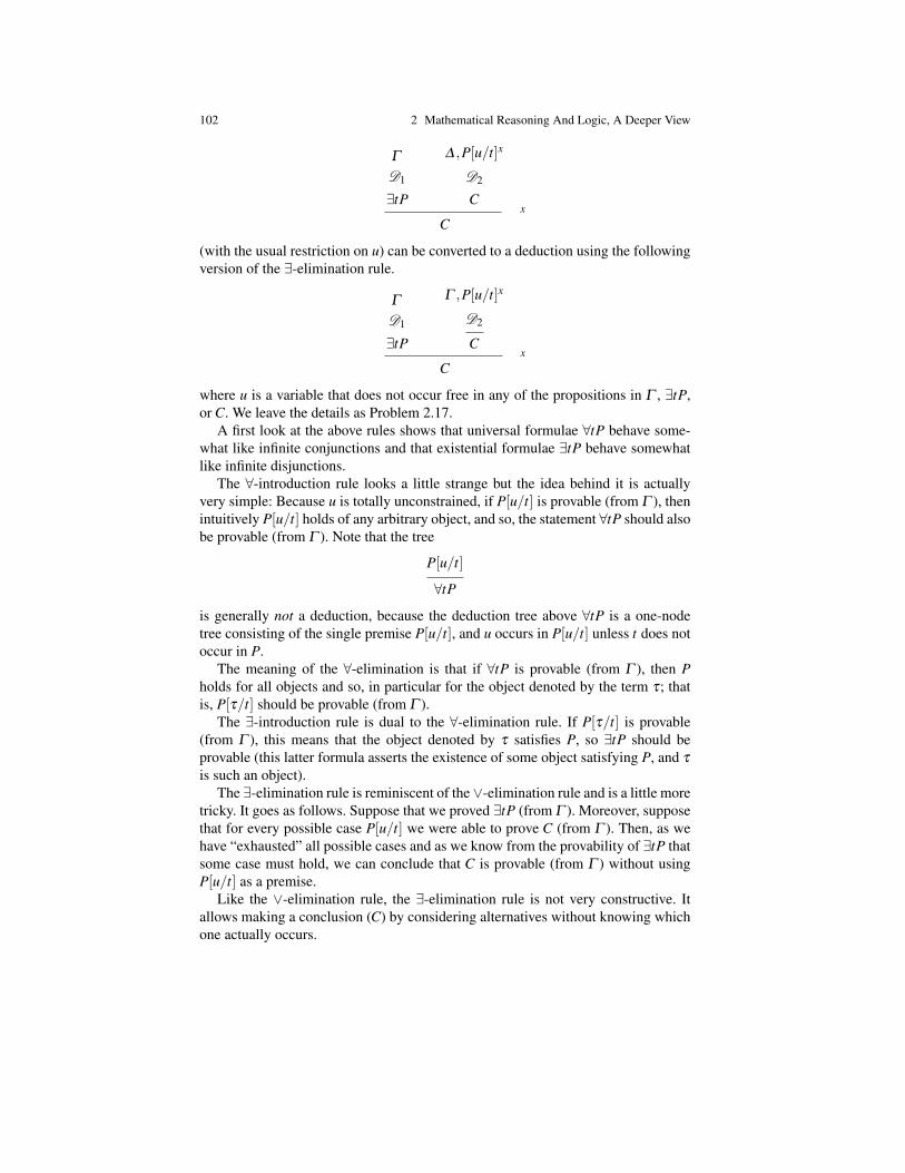
102 2 Mathematical Reasoning And Logic, A Deeper View
Γ
D1
∃tP
∆ ,P[u/t]x
D2
Cx
C
(with the usual restriction on u) can be converted to a deduction using the followingversion of the ∃-elimination rule.
Γ
D1
∃tP
Γ ,P[u/t]x
D2
Cx
C
where u is a variable that does not occur free in any of the propositions in Γ , ∃tP,or C. We leave the details as Problem 2.17.
A first look at the above rules shows that universal formulae ∀tP behave some-what like infinite conjunctions and that existential formulae ∃tP behave somewhatlike infinite disjunctions.
The ∀-introduction rule looks a little strange but the idea behind it is actuallyvery simple: Because u is totally unconstrained, if P[u/t] is provable (from Γ ), thenintuitively P[u/t] holds of any arbitrary object, and so, the statement ∀tP should alsobe provable (from Γ ). Note that the tree
P[u/t]
∀tPis generally not a deduction, because the deduction tree above ∀tP is a one-nodetree consisting of the single premise P[u/t], and u occurs in P[u/t] unless t does notoccur in P.
The meaning of the ∀-elimination is that if ∀tP is provable (from Γ ), then Pholds for all objects and so, in particular for the object denoted by the term τ; thatis, P[τ/t] should be provable (from Γ ).
The ∃-introduction rule is dual to the ∀-elimination rule. If P[τ/t] is provable(from Γ ), this means that the object denoted by τ satisfies P, so ∃tP should beprovable (this latter formula asserts the existence of some object satisfying P, and τ
is such an object).The ∃-elimination rule is reminiscent of the∨-elimination rule and is a little more
tricky. It goes as follows. Suppose that we proved ∃tP (from Γ ). Moreover, supposethat for every possible case P[u/t] we were able to prove C (from Γ ). Then, as wehave “exhausted” all possible cases and as we know from the provability of ∃tP thatsome case must hold, we can conclude that C is provable (from Γ ) without usingP[u/t] as a premise.
Like the ∨-elimination rule, the ∃-elimination rule is not very constructive. Itallows making a conclusion (C) by considering alternatives without knowing whichone actually occurs.

2.9 Adding Quantifiers; The Proof Systems N ⇒,∧,∨,∀,∃,⊥c , N G⇒,∧,∨,∀,∃,⊥
c 103
Remark: Analogously to disjunction, in (first-order) intuitionistic logic, if an exis-tential statement ∃tP is provable, then from any proof of ∃tP, some term τ can beextracted so that P[τ/t] is provable. Such a term τ is called a witness. The witnessproperty is not easy to prove. It follows from the fact that intuitionistic proofs have anormal form (see Section 2.11). However, no such property holds in classical logic(for instance, see the ab rational with a,b irrational example revisited below).
Here is an example of a proof in the system N ⇒,∨,∧,⊥,∀,∃c (actually, in the system
N ⇒,∨,∧,⊥,∀,∃i ) of the formula ∀t(P∧Q)⇒∀tP∧∀tQ.
∀t(P∧Q)x
P[u/t]∧Q[u/t]
P[u/t]
∀tP
∀t(P∧Q)x
P[u/t]∧Q[u/t]
Q[u/t]
∀tQ∀tP∧∀tQ
x
∀t(P∧Q)⇒∀tP∧∀tQIn the above proof, u is a new variable, that is, a variable that does not occur free inP or Q. We also have used some basic properties of substitutions such as
(P∧Q)[τ/t] = P[τ/t]∧Q[τ/t]
(P∨Q)[τ/t] = P[τ/t]∨Q[τ/t]
(P⇒ Q)[τ/t] = P[τ/t]⇒ Q[τ/t]
(¬P)[τ/t] = ¬P[τ/t]
(∀sP)[τ/t] = ∀sP[τ/t]
(∃sP)[τ/t] = ∃sP[τ/t],
for any term τ such that no variable in τ is captured during the substitution (inparticular, in the last two cases, the variable s does not occur in τ).
The reader should show that ∀tP∧∀tQ⇒∀t(P∧Q) is also provable in the systemN ⇒,∨,∧,⊥,∀,∃
i . However, in general, one can’t just replace ∀ by ∃ (or ∧ by ∨) andstill obtain provable statements. For example, ∃tP∧∃tQ⇒∃t(P∧Q) is not provableat all.
Here are some useful equivalences involving quantifiers. The first two are analo-gous to the de Morgan laws for ∧ and ∨.
Proposition 2.10. The following equivalences are provable in classical first-orderlogic.
¬∀tP≡ ∃t¬P
¬∃tP≡ ∀t¬P
∀t(P∧Q)≡ ∀tP∧∀tQ∃t(P∨Q)≡ ∃tP∨∃tQ.
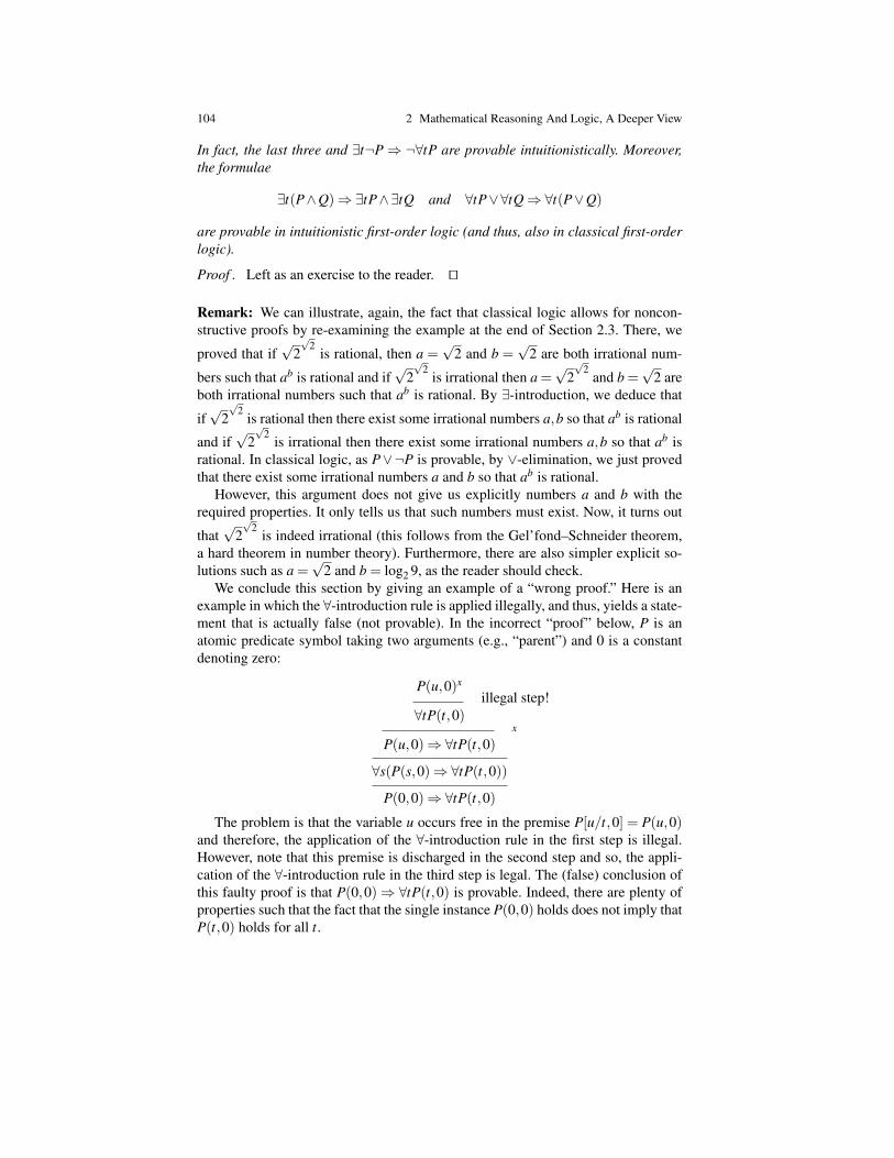
104 2 Mathematical Reasoning And Logic, A Deeper View
In fact, the last three and ∃t¬P⇒ ¬∀tP are provable intuitionistically. Moreover,the formulae
∃t(P∧Q)⇒∃tP∧∃tQ and ∀tP∨∀tQ⇒∀t(P∨Q)
are provable in intuitionistic first-order logic (and thus, also in classical first-orderlogic).
Proof . Left as an exercise to the reader. ut
Remark: We can illustrate, again, the fact that classical logic allows for noncon-structive proofs by re-examining the example at the end of Section 2.3. There, we
proved that if√
2√
2is rational, then a =
√2 and b =
√2 are both irrational num-
bers such that ab is rational and if√
2√
2is irrational then a =
√2√
2and b =
√2 are
both irrational numbers such that ab is rational. By ∃-introduction, we deduce that
if√
2√
2is rational then there exist some irrational numbers a,b so that ab is rational
and if√
2√
2is irrational then there exist some irrational numbers a,b so that ab is
rational. In classical logic, as P∨¬P is provable, by ∨-elimination, we just provedthat there exist some irrational numbers a and b so that ab is rational.
However, this argument does not give us explicitly numbers a and b with therequired properties. It only tells us that such numbers must exist. Now, it turns out
that√
2√
2is indeed irrational (this follows from the Gel’fond–Schneider theorem,
a hard theorem in number theory). Furthermore, there are also simpler explicit so-lutions such as a =
√2 and b = log2 9, as the reader should check.
We conclude this section by giving an example of a “wrong proof.” Here is anexample in which the ∀-introduction rule is applied illegally, and thus, yields a state-ment that is actually false (not provable). In the incorrect “proof” below, P is anatomic predicate symbol taking two arguments (e.g., “parent”) and 0 is a constantdenoting zero:
P(u,0)x
illegal step!∀tP(t,0)
x
P(u,0)⇒∀tP(t,0)∀s(P(s,0)⇒∀tP(t,0))
P(0,0)⇒∀tP(t,0)The problem is that the variable u occurs free in the premise P[u/t,0] = P(u,0)
and therefore, the application of the ∀-introduction rule in the first step is illegal.However, note that this premise is discharged in the second step and so, the appli-cation of the ∀-introduction rule in the third step is legal. The (false) conclusion ofthis faulty proof is that P(0,0)⇒ ∀tP(t,0) is provable. Indeed, there are plenty ofproperties such that the fact that the single instance P(0,0) holds does not imply thatP(t,0) holds for all t.

2.9 Adding Quantifiers; The Proof Systems N ⇒,∧,∨,∀,∃,⊥c , N G⇒,∧,∨,∀,∃,⊥
c 105
Remark: The above example shows why it is desirable to have premises that areuniversally quantified. A premise of the form ∀tP can be instantiated to P[u/t], using∀-elimination, where u is a brand new variable. Later on, it may be possible to use ∀-introduction without running into trouble with free occurrences of u in the premises.But we still have to be very careful when we use ∀-introduction or ∃-elimination.
Before concluding this section, let us give a few more examples of proofs usingthe rules for the quantifiers. First, let us prove that
∀tP≡ ∀uP[u/t],
where u is any variable not free in ∀tP and such that u is not captured during thesubstitution. This rule allows us to rename bound variables (under very mild condi-tions). We have the proofs
(∀tP)α
P[u/t]
∀uP[u/t]α
∀tP⇒∀uP[u/t]
and
(∀uP[u/t])α
P[u/t]
∀tPα
∀uP[u/t]⇒∀tPHere is now a proof (intuitionistic) of
∃t(P⇒ Q)⇒ (∀tP⇒ Q),
where t does not occur (free or bound) in Q.
(∃t(P⇒ Q))z
(P[u/t]⇒ Q)x
(∀tP)y
P[u/t]
Qx
Qy
∀tP⇒ Qz
∃t(P⇒ Q)⇒ (∀tP⇒ Q)
In the above proof, u is a new variable that does not occur in Q, ∀tP, or∃t(P⇒ Q). Because t does not occur in Q, we have
(P⇒ Q)[u/t] = P[u/t]⇒ Q.
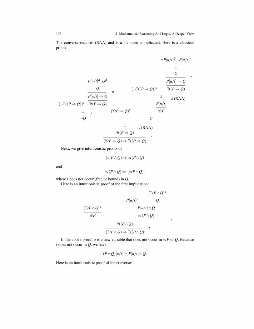
106 2 Mathematical Reasoning And Logic, A Deeper View
The converse requires (RAA) and is a bit more complicated. Here is a classicalproof:
(¬∃t(P⇒ Q))y
P[u/t]α ,Qβ
Qα
P[u/t]⇒ Q
∃t(P⇒ Q)
⊥β
¬Q
(∀tP⇒ Q)x
(¬∃t(P⇒ Q))y
¬P[u/t]δ P[u/t]γ
⊥Q
γ
P[u/t]⇒ Q
∃t(P⇒ Q)
⊥δ (RAA)
P[u/t]
∀tPQ
⊥y (RAA)
∃t(P⇒ Q)x
(∀tP⇒ Q)⇒∃t(P⇒ Q)
Next, we give intuitionistic proofs of
(∃tP∧Q)⇒∃t(P∧Q)
and∃t(P∧Q)⇒ (∃tP∧Q),
where t does not occur (free or bound) in Q.Here is an intuitionistic proof of the first implication:
(∃tP∧Q)x
∃tP
P[u/t]y(∃tP∧Q)x
Q
P[u/t]∧Q
∃t(P∧Q)y
∃t(P∧Q)x
(∃tP∧Q)⇒∃t(P∧Q)
In the above proof, u is a new variable that does not occur in ∃tP or Q. Becauset does not occur in Q, we have
(P∧Q)[u/t] = P[u/t]∧Q.
Here is an intuitionistic proof of the converse:
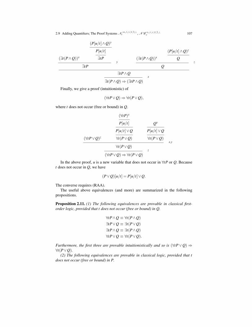
2.9 Adding Quantifiers; The Proof Systems N ⇒,∧,∨,∀,∃,⊥c , N G⇒,∧,∨,∀,∃,⊥
c 107
(∃t(P∧Q))x
(P[u/t]∧Q)y
P[u/t]
∃tPy
∃tP(∃t(P∧Q))x
(P[u/t]∧Q)z
Qz
Q
∃tP∧Qx
∃t(P∧Q)⇒ (∃tP∧Q)
Finally, we give a proof (intuitionistic) of
(∀tP∨Q)⇒∀t(P∨Q),
where t does not occur (free or bound) in Q.
(∀tP∨Q)z
(∀tP)x
P[u/t]
P[u/t]∨Q
∀t(P∨Q)
Qy
P[u/t]∨Q
∀t(P∨Q)x,y
∀t(P∨Q)z
(∀tP∨Q)⇒∀t(P∨Q)
In the above proof, u is a new variable that does not occur in ∀tP or Q. Becauset does not occur in Q, we have
(P∨Q)[u/t] = P[u/t]∨Q.
The converse requires (RAA).The useful above equivalences (and more) are summarized in the following
propositions.
Proposition 2.11. (1) The following equivalences are provable in classical first-order logic, provided that t does not occur (free or bound) in Q.
∀tP∧Q ≡ ∀t(P∧Q)
∃tP∨Q ≡ ∃t(P∨Q)
∃tP∧Q ≡ ∃t(P∧Q)
∀tP∨Q ≡ ∀t(P∨Q).
Furthermore, the first three are provable intuitionistically and so is (∀tP∨Q)⇒∀t(P∨Q).
(2) The following equivalences are provable in classical logic, provided that tdoes not occur (free or bound) in P.

108 2 Mathematical Reasoning And Logic, A Deeper View
∀t(P⇒ Q) ≡ (P⇒∀tQ)
∃t(P⇒ Q) ≡ (P⇒∃tQ).
Furthermore, the first one is provable intuitionistically and so is ∃t(P⇒Q)⇒ (P⇒∃tQ).
(3) The following equivalences are provable in classical logic, provided that tdoes not occur (free or bound) in Q.
∀t(P⇒ Q) ≡ (∃tP⇒ Q)
∃t(P⇒ Q) ≡ (∀tP⇒ Q).
Furthermore, the first one is provable intuitionistically and so is ∃t(P ⇒ Q) ⇒(∀tP⇒ Q).
Proofs that have not been supplied are left as exercises.Obviously, every first-order formula that is provable intuitionistically is also
provable classically and we know that there are formulae that are provable clas-sically but not provable intuitionistically. Therefore, it appears that classical logic ismore general than intuitionistic logic. However, this not not quite so because thereis a way of translating classical logic into intuitionistic logic. To be more precise,every classical formula A can be translated into a formula A∗ where A∗ is classicallyequivalent to A and A is provable classically iff A∗ is provable intuitionistically. Var-ious translations are known, all based on a “trick” involving double-negation (Thisis because ¬¬¬A and ¬A are intuitionistically equivalent). Translations were givenby Kolmogorov (1925), Godel (1933), and Gentzen (1933).
Fig. 2.4 Andrey N. Kolmogorov, 1903–1987 (left) and Kurt Godel, 1906–1978 (right)
For example, Godel used the following translation.

2.10 First-Order Theories 109
A∗ = ¬¬A, if A is atomic,(¬A)∗ = ¬A∗,
(A∧B)∗ = (A∗∧B∗),
(A⇒ B)∗ = ¬(A∗∧¬B∗),
(A∨B)∗ = ¬(¬A∗∧¬B∗),
(∀xA)∗ = ∀xA∗,
(∃xA)∗ = ¬∀x¬A∗.
Actually, if we restrict our attention to propositions (i.e., formulae without quan-tifiers), a theorem of V. Glivenko (1929) states that if a proposition A is provableclassically, then ¬¬A is provable intuitionistically. In view of these results, the pro-ponents of intuitionistic logic claim that classical logic is really a special case ofintuitionistic logic. However, the above translations have some undesirable proper-ties, as noticed by Girard. For more details on all this, see Gallier [5].
2.10 First-Order Theories
The way we presented deduction trees and proof trees may have given our readersthe impression that the set of premises Γ was just an auxiliary notion. Indeed, inall of our examples, Γ ends up being empty. However, nonempty Γ s are cruciallyneeded if we want to develop theories about various kinds of structures and objects,such as the natural numbers, groups, rings, fields, trees, graphs, sets, and the like.Indeed, we need to make definitions about the objects we want to study and we needto state some axioms asserting the main properties of these objects. We do this byputting these definitions and axioms in Γ . Actually, we have to allow Γ to be infinitebut we still require that our deduction trees be finite; they can only use finitely manyof the formulae in Γ . We are then interested in all formulae P such that ∆ → P isprovable, where ∆ is any finite subset of Γ ; the set of all such Ps is called a theory(or first-order theory). Of course we have the usual problem of consistency: if weare not careful, our theory may be inconsistent, that is, it may consist of all formulae.
Let us give two examples of theories.Our first example is the theory of equality. Indeed, our readers may have noticed
that we have avoided dealing with the equality relation. In practice, we can’t do that.Given a language L with a given supply of constant, function, and predicate
symbols, the theory of equality consists of the following formulae taken as axioms.
∀x(x = x)
∀x1 · · ·∀xn∀y1 · · ·∀yn[(x1 = y1∧·· ·∧ xn = yn)⇒ f (x1, . . . ,xn) = f (y1, . . . ,yn)]
∀x1 · · ·∀xn∀y1 · · ·∀yn[(x1 = y1∧·· ·∧ xn = yn)∧P(x1, . . . ,xn)⇒ P(y1, . . . ,yn)],
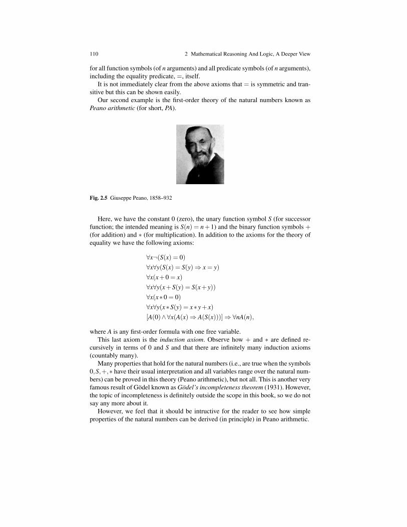
110 2 Mathematical Reasoning And Logic, A Deeper View
for all function symbols (of n arguments) and all predicate symbols (of n arguments),including the equality predicate, =, itself.
It is not immediately clear from the above axioms that = is symmetric and tran-sitive but this can be shown easily.
Our second example is the first-order theory of the natural numbers known asPeano arithmetic (for short, PA).
Fig. 2.5 Giuseppe Peano, 1858–932
Here, we have the constant 0 (zero), the unary function symbol S (for successorfunction; the intended meaning is S(n) = n+1) and the binary function symbols +(for addition) and ∗ (for multiplication). In addition to the axioms for the theory ofequality we have the following axioms:
∀x¬(S(x) = 0)∀x∀y(S(x) = S(y)⇒ x = y)
∀x(x+0 = x)
∀x∀y(x+S(y) = S(x+ y))
∀x(x∗0 = 0)∀x∀y(x∗S(y) = x∗ y+ x)
[A(0)∧∀x(A(x)⇒ A(S(x)))]⇒∀nA(n),
where A is any first-order formula with one free variable.This last axiom is the induction axiom. Observe how + and ∗ are defined re-
cursively in terms of 0 and S and that there are infinitely many induction axioms(countably many).
Many properties that hold for the natural numbers (i.e., are true when the symbols0,S,+,∗ have their usual interpretation and all variables range over the natural num-bers) can be proved in this theory (Peano arithmetic), but not all. This is another veryfamous result of Godel known as Godel’s incompleteness theorem (1931). However,the topic of incompleteness is definitely outside the scope in this book, so we do notsay any more about it.
However, we feel that it should be intructive for the reader to see how simpleproperties of the natural numbers can be derived (in principle) in Peano arithmetic.
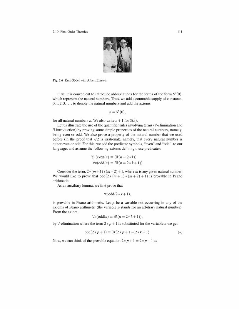
2.10 First-Order Theories 111
Fig. 2.6 Kurt Godel with Albert Einstein
First, it is convenient to introduce abbreviations for the terms of the form Sn(0),which represent the natural numbers. Thus, we add a countable supply of constants,0,1,2,3, . . . , to denote the natural numbers and add the axioms
n = Sn(0),
for all natural numbers n. We also write n+1 for S(n).Let us illustrate the use of the quantifier rules involving terms (∀-elimination and
∃-introduction) by proving some simple properties of the natural numbers, namely,being even or odd. We also prove a property of the natural number that we usedbefore (in the proof that
√2 is irrational), namely, that every natural number is
either even or odd. For this, we add the predicate symbols, “even” and “odd”, to ourlanguage, and assume the following axioms defining these predicates:
∀n(even(n) ≡ ∃k(n = 2∗ k))
∀n(odd(n) ≡ ∃k(n = 2∗ k+1)).
Consider the term, 2∗(m+1)∗(m+2)+1, where m is any given natural number.We would like to prove that odd(2 ∗ (m+ 1) ∗ (m+ 2) + 1) is provable in Peanoarithmetic.
As an auxiliary lemma, we first prove that
∀xodd(2∗ x+1),
is provable in Peano arithmetic. Let p be a variable not occurring in any of theaxioms of Peano arithmetic (the variable p stands for an arbitrary natural number).From the axiom,
∀n(odd(n)≡ ∃k(n = 2∗ k+1)),
by ∀-elimination where the term 2∗ p+1 is substituted for the variable n we get
odd(2∗ p+1)≡ ∃k(2∗ p+1 = 2∗ k+1). (∗)
Now, we can think of the provable equation 2∗ p+1 = 2∗ p+1 as
112 2 Mathematical Reasoning And Logic, A Deeper View
(2∗ p+1 = 2∗ k+1)[p/k],
so, by ∃-introduction, we can conclude that
∃k(2∗ p+1 = 2∗ k+1),
which, by (∗), implies thatodd(2∗ p+1).
But now, because p is a variable not occurring free in the axioms of Peano arith-metic, by ∀-introduction, we conclude that
∀xodd(2∗ x+1).
Finally, if we use ∀-elimination where we substitute the term, τ = (m+1)∗ (m+2),for x, we get
odd(2∗ (m+1)∗ (m+2)+1),
as claimed.Now, we wish to prove the formula:
∀n(even(n)∨odd(n)).
We use the induction principle of Peano arithmetic with
A(n) = even(n)∨odd(n).
For the base case, n = 0, because 0 = 2∗0 (which can be proved from the Peanoaxioms), we see that even(0) holds and so even(0)∨odd(0) is proved.
For n = 1, because 1 = 2∗0+1 (which can be proved from the Peano axioms),we see that odd(1) holds and so even(1)∨odd(1) is proved.
For the induction step, we may assume that A(n) has been proved and we needto prove that A(n+1) holds.
So, assume that even(n)∨odd(n) holds. We do a proof by cases.(a) If even(n) holds, by definition this means that n = 2k for some k and then,
n+1 = 2k+1, which again, by definition means that odd(n+1) holds and thus,even(n+1)∨odd(n+1) holds.
(b) If odd(n) holds, by definition this means that n = 2k+1 for some k and then,n+1 = 2k+2 = 2(k+1), which again, by definition means that even(n+1) holdsand thus, even(n+1)∨odd(n+1) holds.
By ∨-elimination, we conclude that even(n+1)∨odd(n+1) holds, establishingthe induction step.
Therefore, using induction, we have proved that
∀n(even(n)∨odd(n)).
Actually, we know that even(n) and odd(n) are mutually exclusive, which meansthat

2.10 First-Order Theories 113
∀n¬(even(n)∧odd(n))
holds, but how do we prove it?We can do this using induction. For n = 0, the statement odd(0) means that
0 = 2k+1 = S(2k), for some k. However, the first axiom of Peano arithmetic statesthat S(x) 6= 0 for all x, so we get a contradiction.
For the induction step, assume that ¬(even(n)∧odd(n)) holds. We need to provethat ¬(even(n+1)∧odd(n+1)) holds and we can do this by using our constructiveproof-by-contradiction rule. So, assume that even(n+1)∧odd(n+1) holds. At thisstage, we realize that if we could prove that
∀n(even(n+1)⇒ odd(n)) (∗)
and∀n(odd(n+1)⇒ even(n)) (∗∗)
then even(n+1)∧odd(n+1) would imply even(n)∧odd(n), contradicting the as-sumption ¬(even(n)∧odd(n)). Therefore, the proof is complete if we can prove (∗)and (∗∗).
Let’s consider the implication (∗) leaving the proof of (∗∗) as an exercise.Assume that even(n+1) holds. Then, n+1 = 2k, for some natural number k. We
can’t have k = 0 because otherwise we would have n+1 = 0, contradicting one ofthe Peano axioms. But then, k is of the form k = h+1, for some natural number, h,so
n+1 = 2k = 2(h+1) = 2h+2 = (2h+1)+1.
By the second Peano axiom, we must have
n = 2h+1,
which proves that n is odd, as desired.In that last proof, we made implicit use of the fact that every natural number n
different from zero is of the form n = m+ 1, for some natural number m which isformalized as
∀n((n 6= 0)⇒∃m(n = m+1)).
This is easily proved by induction.Having done all this work, we have finally proved (∗) and after proving (∗∗), we
will have proved that∀n¬(even(n)∧odd(n)).
It is also easy to prove that
∀n(even(n)∨odd(n))
and∀n¬(even(n)∧odd(n))
together imply that
114 2 Mathematical Reasoning And Logic, A Deeper View
∀n(even(n)≡ ¬odd(n)) and ∀n(odd(n)≡ ¬even(n)),
are provable, facts that we used several times in Section 2.6. This is because, if
∀x(P∨Q) and ∀x¬(P∧Q)
can be deduced intuitionistically from a set of premises, Γ , then
∀x(P≡ ¬Q) and ∀x(Q≡ ¬P)
can also be deduced intuitionistically from Γ . It also follows that ∀x(¬¬P≡ P) and∀x(¬¬Q≡ Q) can be deduced intuitionistically from Γ .
Remark: Even though we proved that every nonzero natural number n is of theform n = m+ 1, for some natural number m, the expression n− 1 does not makesense because the predecessor function n 7→ n− 1 has not been defined yet in ourlogical system. We need to define a function symbol “pred” satisfying the axioms:
pred(0) = 0∀n(pred(n+1) = n).
For simplicity of notation, we write n−1 instead of pred(n). Then, we can prove thatif k 6= 0, then 2k− 1 = 2(k− 1)+ 1 (which really should be written as pred(2k) =2pred(k) + 1). This can indeed be done by induction; we leave the details as anexercise. We can also define substraction, −, as a function sastisfying the axioms
∀n(n−0 = n)
∀n∀m(n− (m+1) = pred(n−m)).
It is then possible to prove the usual properties of subtraction (by induction).These examples of proofs in the theory of Peano arithmetic illustrate the fact that
constructing proofs in an axiomatized theory is a very laborious and tedious process.Many small technical lemmas need to be established from the axioms, which rendersthese proofs very lengthy and often unintuitive. It is therefore important to build up adatabase of useful basic facts if we wish to prove, with a certain amount of comfort,properties of objects whose properties are defined by an axiomatic theory (such asthe natural numbers). However, when in doubt, we can always go back to the formaltheory and try to prove rigorously the facts that we are not sure about, even thoughthis is usually a tedious and painful process. Human provers navigate in a “spectrumof formality,” most of the time constructing informal proofs containing quite a few(harmless) shortcuts, sometimes making extra efforts to construct more formalizedand rigorous arguments if the need arises.
Now, what if the theory of Peano arithmetic were inconsistent! How do knowthat Peano arithmetic does not imply any contradiction? This is an important andhard question that motivated a lot of the work of Gentzen. An easy answer is that thestandard model N of the natural numbers under addition and multiplication validatesall the axioms of Peano arithmetic. Therefore, if both P and ¬P could be proved

2.11 Decision Procedures, Proof Normalization, Counterexamples 115
from the Peano axioms, then both P and ¬P would be true in N, which is absurd. Tomake all this rigorous, we need to define the notion of truth in a structure, a notionexplained in every logic book. It should be noted that the constructivists will objectto the above method for showing the consistency of Peano arithmetic, because itassumes that the infinite set N exists as a completed entity. Until further notice, wehave faith in the consistency of Peano arithmetic (so far, no inconsistency has beenfound).
Another very interesting theory is set theory. There are a number of axiomatiza-tions of set theory and we discuss one of them (ZF) very briefly in Section 2.12.
Several times in this chapter, we have claimed that certain formulae are not prov-able in some logical system. What kind of reasoning do we use to validate suchclaims? In the next section, we briefly address this question as well as related ones.
2.11 Decision Procedures, Proof Normalization,Counterexamples
In the previous sections, we saw how the rules of mathematical reasoning can beformalized in various natural deduction systems and we defined a precise notion ofproof. We observed that finding a proof for a given proposition was not a simplematter, nor was it to acertain that a proposition is unprovable. Thus, it is natural toask the following question.
The Decision Problem: Is there a general procedure that takes any arbitraryproposition P as input, always terminates in a finite number of steps, and tells uswhether P is provable?
Clearly, it would be very nice if such a procedure existed, especially if it alsoproduced a proof of P when P is provable.
Unfortunately, for rich enough languages, such as first-order logic, it is impos-sible to find such a procedure. This deep result known as the undecidability of thedecision problem or Church’s theorem was proved by A. Church in 1936 (actually,Church proved the undecidability of the validity problem but, by Godel’s complete-ness theorem, validity and provability are equivalent).
Fig. 2.7 Alonzo Church, 1903–1995 (left) and Alan Turing, 1912–1954 (right)
116 2 Mathematical Reasoning And Logic, A Deeper View
Proving Church’s theorem is hard and a lot of work. One needs to develop a gooddeal of what is called the theory of computation. This involves defining models ofcomputation such as Turing machines and proving other deep results such as theundecidability of the halting problem and the undecidability of the Post correspon-dence problem, among other things, see Hopcroft, Motwani, and Ullman [12] andLewis and Papadimitriou [16].
So, our hopes to find a “universal theorem prover” are crushed. However, if werestrict ourselves to propositional logic, classical or intuitionistic, it turns out thatprocedures solving the decision problem do exist and they even produce a proof ofthe input proposition when that proposition is provable.
Unfortunately, proving that such procedures exist and are correct in the proposi-tional case is rather difficult, especially for intuitionistic logic. The difficulties havea lot to do with our choice of a natural deduction system. Indeed, even for the sys-tem N ⇒
m (or N G⇒m ), provable propositions may have infinitely many proofs. Thismakes the search process impossible; when do we know how to stop, especially ifa proposition is not provable. The problem is that proofs may contain redundancies(Gentzen said “detours”). A typical example of redundancy is when an eliminationimmediately follows an introduction, as in the following example in which D1 de-notes a deduction with conclusion Γ ,x : A→ B and D2 denotes a deduction withconclusion Γ → A.
D1
Γ ,x : A→ B
Γ → A⇒ B
D2
Γ → A
Γ → B
Intuitively, it should be possible to construct a deduction for Γ → B from thetwo deductions D1 and D2 without using at all the hypothesis x : A. This is indeedthe case. If we look closely at the deduction D1, from the shape of the inferencerules, assumptions are never created, and the leaves must be labeled with expres-sions of the form Γ ′,∆ ,x : A,y : C→C or Γ ,∆ ,x : A→ A, where y 6= x and eitherΓ = Γ ′ or Γ = Γ ′,y : C. We can form a new deduction for Γ → B as follows. InD1, wherever a leaf of the form Γ ,∆ ,x : A→ A occurs, replace it by the deductionobtained from D2 by adding ∆ to the premise of each sequent in D2. Actually, oneshould be careful to first make a fresh copy of D2 by renaming all the variables sothat clashes with variables in D1 are avoided. Finally, delete the assumption x : Afrom the premise of every sequent in the resulting proof. The resulting deduction isobtained by a kind of substitution and may be denoted as D1[D2/x], with some mi-nor abuse of notation. Note that the assumptions x : A occurring in the leaves of theform Γ ′,∆ ,x : A,y : C→C were never used anyway. The step that consists in trans-forming the above redundant proof figure into the deduction D1[D2/x] is called areduction step or normalization step.
The idea of proof normalization goes back to Gentzen ([7], 1935). Gentzen notedthat (formal) proofs can contain redundancies, or “detours,” and that most complica-tions in the analysis of proofs are due to these redundancies. Thus, Gentzen had the
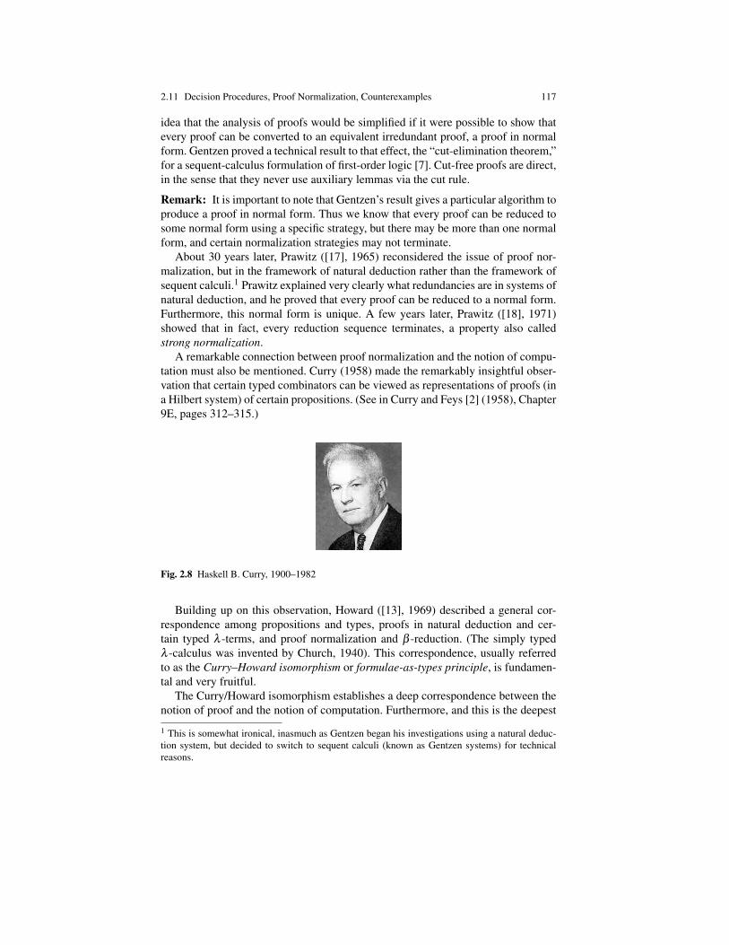
2.11 Decision Procedures, Proof Normalization, Counterexamples 117
idea that the analysis of proofs would be simplified if it were possible to show thatevery proof can be converted to an equivalent irredundant proof, a proof in normalform. Gentzen proved a technical result to that effect, the “cut-elimination theorem,”for a sequent-calculus formulation of first-order logic [7]. Cut-free proofs are direct,in the sense that they never use auxiliary lemmas via the cut rule.
Remark: It is important to note that Gentzen’s result gives a particular algorithm toproduce a proof in normal form. Thus we know that every proof can be reduced tosome normal form using a specific strategy, but there may be more than one normalform, and certain normalization strategies may not terminate.
About 30 years later, Prawitz ([17], 1965) reconsidered the issue of proof nor-malization, but in the framework of natural deduction rather than the framework ofsequent calculi.1 Prawitz explained very clearly what redundancies are in systems ofnatural deduction, and he proved that every proof can be reduced to a normal form.Furthermore, this normal form is unique. A few years later, Prawitz ([18], 1971)showed that in fact, every reduction sequence terminates, a property also calledstrong normalization.
A remarkable connection between proof normalization and the notion of compu-tation must also be mentioned. Curry (1958) made the remarkably insightful obser-vation that certain typed combinators can be viewed as representations of proofs (ina Hilbert system) of certain propositions. (See in Curry and Feys [2] (1958), Chapter9E, pages 312–315.)
Fig. 2.8 Haskell B. Curry, 1900–1982
Building up on this observation, Howard ([13], 1969) described a general cor-respondence among propositions and types, proofs in natural deduction and cer-tain typed λ -terms, and proof normalization and β -reduction. (The simply typedλ -calculus was invented by Church, 1940). This correspondence, usually referredto as the Curry–Howard isomorphism or formulae-as-types principle, is fundamen-tal and very fruitful.
The Curry/Howard isomorphism establishes a deep correspondence between thenotion of proof and the notion of computation. Furthermore, and this is the deepest
1 This is somewhat ironical, inasmuch as Gentzen began his investigations using a natural deduc-tion system, but decided to switch to sequent calculi (known as Gentzen systems) for technicalreasons.
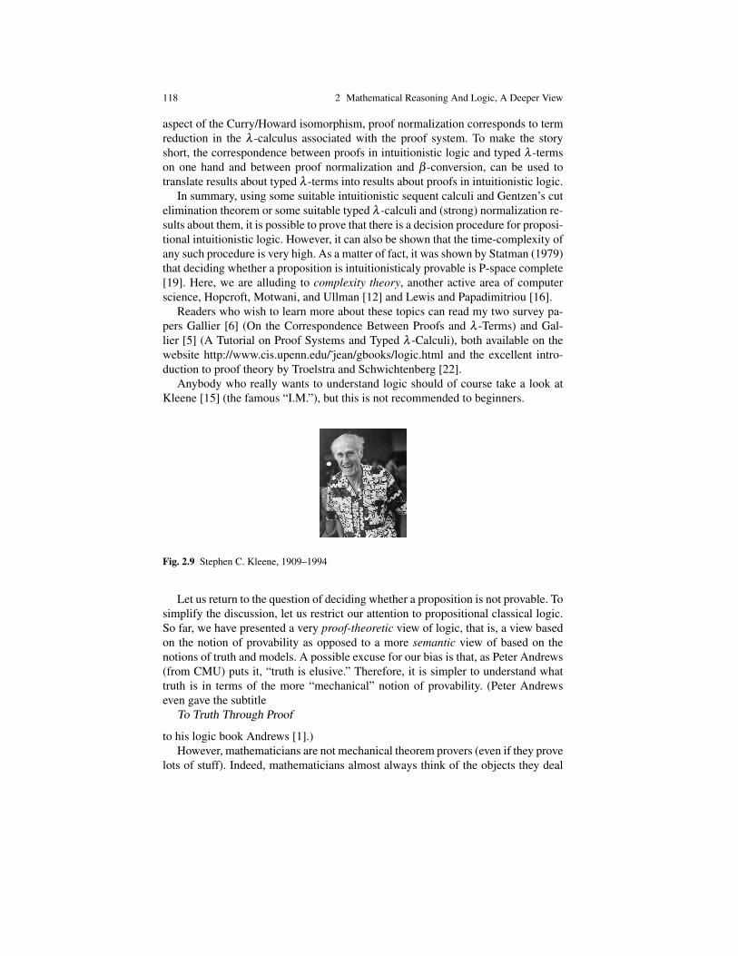
118 2 Mathematical Reasoning And Logic, A Deeper View
aspect of the Curry/Howard isomorphism, proof normalization corresponds to termreduction in the λ -calculus associated with the proof system. To make the storyshort, the correspondence between proofs in intuitionistic logic and typed λ -termson one hand and between proof normalization and β -conversion, can be used totranslate results about typed λ -terms into results about proofs in intuitionistic logic.
In summary, using some suitable intuitionistic sequent calculi and Gentzen’s cutelimination theorem or some suitable typed λ -calculi and (strong) normalization re-sults about them, it is possible to prove that there is a decision procedure for proposi-tional intuitionistic logic. However, it can also be shown that the time-complexity ofany such procedure is very high. As a matter of fact, it was shown by Statman (1979)that deciding whether a proposition is intuitionisticaly provable is P-space complete[19]. Here, we are alluding to complexity theory, another active area of computerscience, Hopcroft, Motwani, and Ullman [12] and Lewis and Papadimitriou [16].
Readers who wish to learn more about these topics can read my two survey pa-pers Gallier [6] (On the Correspondence Between Proofs and λ -Terms) and Gal-lier [5] (A Tutorial on Proof Systems and Typed λ -Calculi), both available on thewebsite http://www.cis.upenn.edu/ jean/gbooks/logic.html and the excellent intro-duction to proof theory by Troelstra and Schwichtenberg [22].
Anybody who really wants to understand logic should of course take a look atKleene [15] (the famous “I.M.”), but this is not recommended to beginners.
Fig. 2.9 Stephen C. Kleene, 1909–1994
Let us return to the question of deciding whether a proposition is not provable. Tosimplify the discussion, let us restrict our attention to propositional classical logic.So far, we have presented a very proof-theoretic view of logic, that is, a view basedon the notion of provability as opposed to a more semantic view of based on thenotions of truth and models. A possible excuse for our bias is that, as Peter Andrews(from CMU) puts it, “truth is elusive.” Therefore, it is simpler to understand whattruth is in terms of the more “mechanical” notion of provability. (Peter Andrewseven gave the subtitle
To Truth Through Proof
to his logic book Andrews [1].)However, mathematicians are not mechanical theorem provers (even if they prove
lots of stuff). Indeed, mathematicians almost always think of the objects they deal
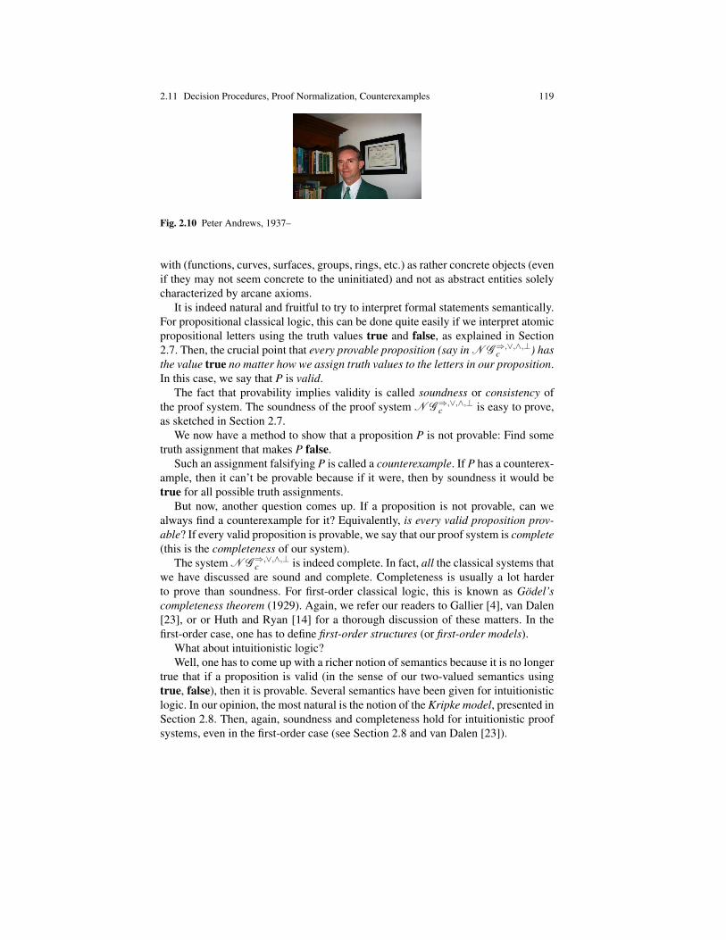
2.11 Decision Procedures, Proof Normalization, Counterexamples 119
Fig. 2.10 Peter Andrews, 1937–
with (functions, curves, surfaces, groups, rings, etc.) as rather concrete objects (evenif they may not seem concrete to the uninitiated) and not as abstract entities solelycharacterized by arcane axioms.
It is indeed natural and fruitful to try to interpret formal statements semantically.For propositional classical logic, this can be done quite easily if we interpret atomicpropositional letters using the truth values true and false, as explained in Section2.7. Then, the crucial point that every provable proposition (say in N G⇒,∨,∧,⊥
c ) hasthe value true no matter how we assign truth values to the letters in our proposition.In this case, we say that P is valid.
The fact that provability implies validity is called soundness or consistency ofthe proof system. The soundness of the proof system N G⇒,∨,∧,⊥
c is easy to prove,as sketched in Section 2.7.
We now have a method to show that a proposition P is not provable: Find sometruth assignment that makes P false.
Such an assignment falsifying P is called a counterexample. If P has a counterex-ample, then it can’t be provable because if it were, then by soundness it would betrue for all possible truth assignments.
But now, another question comes up. If a proposition is not provable, can wealways find a counterexample for it? Equivalently, is every valid proposition prov-able? If every valid proposition is provable, we say that our proof system is complete(this is the completeness of our system).
The system N G⇒,∨,∧,⊥c is indeed complete. In fact, all the classical systems that
we have discussed are sound and complete. Completeness is usually a lot harderto prove than soundness. For first-order classical logic, this is known as Godel’scompleteness theorem (1929). Again, we refer our readers to Gallier [4], van Dalen[23], or or Huth and Ryan [14] for a thorough discussion of these matters. In thefirst-order case, one has to define first-order structures (or first-order models).
What about intuitionistic logic?Well, one has to come up with a richer notion of semantics because it is no longer
true that if a proposition is valid (in the sense of our two-valued semantics usingtrue, false), then it is provable. Several semantics have been given for intuitionisticlogic. In our opinion, the most natural is the notion of the Kripke model, presented inSection 2.8. Then, again, soundness and completeness hold for intuitionistic proofsystems, even in the first-order case (see Section 2.8 and van Dalen [23]).
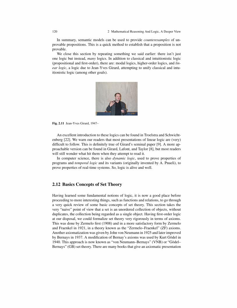
120 2 Mathematical Reasoning And Logic, A Deeper View
In summary, semantic models can be used to provide counterexamples of un-provable propositions. This is a quick method to establish that a proposition is notprovable.
We close this section by repeating something we said earlier: there isn’t justone logic but instead, many logics. In addition to classical and intuitionistic logic(propositional and first-order), there are: modal logics, higher-order logics, and lin-ear logic, a logic due to Jean-Yves Girard, attempting to unify classical and intu-itionistic logic (among other goals).
Fig. 2.11 Jean-Yves Girard, 1947–
An excellent introduction to these logics can be found in Troelstra and Schwicht-enberg [22]. We warn our readers that most presentations of linear logic are (very)difficult to follow. This is definitely true of Girard’s seminal paper [9]. A more ap-proachable version can be found in Girard, Lafont, and Taylor [8], but most readerswill still wonder what hit them when they attempt to read it.
In computer science, there is also dynamic logic, used to prove properties ofprograms and temporal logic and its variants (originally invented by A. Pnueli), toprove properties of real-time systems. So, logic is alive and well.
2.12 Basics Concepts of Set Theory
Having learned some fundamental notions of logic, it is now a good place beforeproceeding to more interesting things, such as functions and relations, to go througha very quick review of some basic concepts of set theory. This section takes thevery “naive” point of view that a set is an unordered collection of objects, withoutduplicates, the collection being regarded as a single object. Having first-order logicat our disposal, we could formalize set theory very rigorously in terms of axioms.This was done by Zermelo first (1908) and in a more satisfactory form by Zermeloand Fraenkel in 1921, in a theory known as the “Zermelo–Fraenkel” (ZF) axioms.Another axiomatization was given by John von Neumann in 1925 and later improvedby Bernays in 1937. A modification of Bernay’s axioms was used by Kurt Godel in1940. This approach is now known as “von Neumann–Bernays” (VNB) or “Godel–Bernays” (GB) set theory. There are many books that give an axiomatic presentation
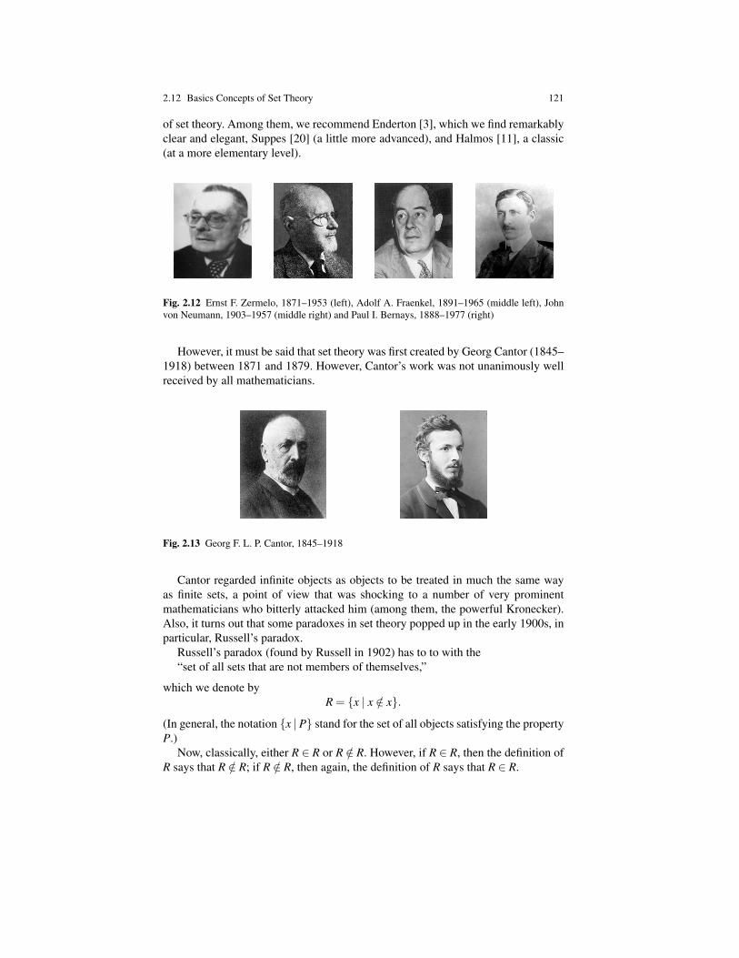
2.12 Basics Concepts of Set Theory 121
of set theory. Among them, we recommend Enderton [3], which we find remarkablyclear and elegant, Suppes [20] (a little more advanced), and Halmos [11], a classic(at a more elementary level).
Fig. 2.12 Ernst F. Zermelo, 1871–1953 (left), Adolf A. Fraenkel, 1891–1965 (middle left), Johnvon Neumann, 1903–1957 (middle right) and Paul I. Bernays, 1888–1977 (right)
However, it must be said that set theory was first created by Georg Cantor (1845–1918) between 1871 and 1879. However, Cantor’s work was not unanimously wellreceived by all mathematicians.
Fig. 2.13 Georg F. L. P. Cantor, 1845–1918
Cantor regarded infinite objects as objects to be treated in much the same wayas finite sets, a point of view that was shocking to a number of very prominentmathematicians who bitterly attacked him (among them, the powerful Kronecker).Also, it turns out that some paradoxes in set theory popped up in the early 1900s, inparticular, Russell’s paradox.
Russell’s paradox (found by Russell in 1902) has to to with the“set of all sets that are not members of themselves,”
which we denote byR = x | x /∈ x.
(In general, the notation x | P stand for the set of all objects satisfying the propertyP.)
Now, classically, either R ∈ R or R /∈ R. However, if R ∈ R, then the definition ofR says that R /∈ R; if R /∈ R, then again, the definition of R says that R ∈ R.
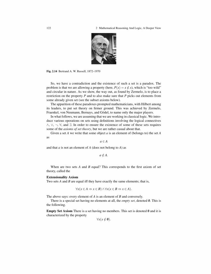
122 2 Mathematical Reasoning And Logic, A Deeper View
Fig. 2.14 Bertrand A. W. Russell, 1872–1970
So, we have a contradiction and the existence of such a set is a paradox. Theproblem is that we are allowing a property (here, P(x) = x /∈ x), which is “too wild”and circular in nature. As we show, the way out, as found by Zermelo, is to place arestriction on the property P and to also make sure that P picks out elements fromsome already given set (see the subset axioms below).
The apparition of these paradoxes prompted mathematicians, with Hilbert amongits leaders, to put set theory on firmer ground. This was achieved by Zermelo,Fraenkel, von Neumann, Bernays, and Godel, to name only the major players.
In what follows, we are assuming that we are working in classical logic. We intro-duce various operations on sets using definitions involving the logical connectives∧, ∨, ¬, ∀, and ∃. In order to ensure the existence of some of these sets requiressome of the axioms of set theory, but we are rather casual about that.
Given a set A we write that some object a is an element of (belongs to) the set Aas
a ∈ A
and that a is not an element of A (does not belong to A) as
a /∈ A.
When are two sets A and B equal? This corresponds to the first axiom of settheory, called the
Extensionality AxiomTwo sets A and B are equal iff they have exactly the same elements; that is,
∀x(x ∈ A⇒ x ∈ B)∧∀x(x ∈ B⇒ x ∈ A).
The above says: every element of A is an element of B and conversely.There is a special set having no elements at all, the empty set, denoted /0. This is
the following.
Empty Set Axiom There is a set having no members. This set is denoted /0 and it ischaracterized by the property
∀x(x /∈ /0).

2.12 Basics Concepts of Set Theory 123
Remark: Beginners often wonder whether there is more than one empty set. Forexample, is the empty set of professors distinct from the empty set of potatoes?
The answer is, by the extensionality axiom, there is only one empty set.Given any two objects a and b, we can form the set a,b containing exactly
these two objects. Amazingly enough, this must also be an axiom:
Pairing AxiomGiven any two objects a and b (think sets), there is a set a,b having as membersjust a and b.
Observe that if a and b are identical, then we have the set a,a, which is denotedby a and is called a singleton set (this set has a as its only element).
To form bigger sets, we use the union operation. This too requires an axiom.
Union Axiom (Version 1)For any two sets A and B, there is a set A∪B called the union of A and B defined by
x ∈ A∪B iff (x ∈ A)∨ (x ∈ B).
This reads, x is a member of A∪B if either x belongs to A or x belongs to B (orboth). We also write
A∪B = x | x ∈ A or x ∈ B.Using the union operation, we can form bigger sets by taking unions with singletons.For example, we can form
a,b,c= a,b∪c.
Remark: We can systematically construct bigger and bigger sets by the followingmethod: Given any set A let
A+ = A∪A.If we start from the empty set, we obtain sets that can be used to define the naturalnumbers and the + operation corresponds to the successor function on the naturalnumbers (i.e., n 7→ n+1).
Another operation is the power set formation. It is indeed a “powerful” operation,in the sense that it allows us to form very big sets. For this, it is helpful to definethe notion of inclusion between sets. Given any two sets, A and B, we say that A isa subset of B (or that A is included in B), denoted A ⊆ B, iff every element of A isalso an element of B, that is,
∀x(x ∈ A⇒ x ∈ B).
We say that A is a proper subset of B iff A ⊆ B and A 6= B. This implies that thatthere is some b ∈ B with b /∈ A. We usually write A⊂ B.
Observe that the equality of two sets can be expressed by
A = B iff A⊆ B and B⊆ A.

124 2 Mathematical Reasoning And Logic, A Deeper View
Power Set AxiomGiven any set A, there is a set P(A) (also denoted 2A) called the power set of Awhose members are exactly the subsets of A; that is,
X ∈P(A) iff X ⊆ A.
For example, if A = a,b,c, then
P(A) = /0,a,b,c,a,b,a,c,b,c,a,b,c,
a set containing eight elements. Note that the empty set and A itself are alwaysmembers of P(A).
Remark: If A has n elements, it is not hard to show that P(A) has 2n elements.For this reason, many people, including me, prefer the notation 2A for the power setof A.
At this stage, we define intersection and complementation. For this, given anyset A and given a property P (specified by a first-order formula) we need to be ableto define the subset of A consisting of those elements satisfying P. This subset isdenoted by
x ∈ A | P.Unfortunately, there are problems with this construction. If the formula P is some-how a circular definition and refers to the subset that we are trying to define, thensome paradoxes may arise.
The way out is to place a restriction on the formula used to define our subsets,and this leads to the subset axioms, first formulated by Zermelo. These axioms arealso called comprehension axioms or axioms of separation.
Subset AxiomsFor every first-order formula P we have the axiom:
∀A∃X∀x(x ∈ X iff (x ∈ A)∧P),
where P does not contain X as a free variable. (However, P may contain x free.)The subset axioms says that for every set A there is a set X consisting exactly of
those elements of A so that P holds. For short, we usually write
X = x ∈ A | P.
As an example, consider the formula
P(B,x) = x ∈ B.
Then, the subset axiom says
∀A∃X∀x(x ∈ A∧ x ∈ B),
2.12 Basics Concepts of Set Theory 125
which means that X is the set of elements that belong both to A and B. This is calledthe intersection of A and B, denoted by A∩B. Note that
A∩B = x | x ∈ A and x ∈ B.
We can also define the relative complement of B in A, denoted A−B, given bythe formula P(B,x) = x /∈ B, so that
A−B = x | x ∈ A and x /∈ B.
In particular, if A is any given set and B is any subset of A, the set A−B is alsodenoted B and is called the complement of B.
The algebraic properties of union, intersection, and complementation are inher-ited from the properties of disjunction, conjunction, and negation. The followingproposition lists some of the most important properties of union, intersection, andcomplementation.
Proposition 2.12. The following equations hold for all sets A,B,C:
A∪ /0 = A
A∩ /0 = /0A∪A = A
A∩A = A
A∪B = B∪A
A∩B = B∩A.
The last two assert the commutativity of ∪ and ∩. We have distributivity of ∩ over ∪and of ∪ over ∩:
A∩ (B∪C) = (A∩B)∪ (A∩C)
A∪ (B∩C) = (A∪B)∩ (A∪C).
We have associativity of ∩ and ∪:
A∩ (B∩C) = (A∩B)∩C
A∪ (B∪C) = (A∪B)∪C.
Proof . Use Proposition 2.5.
Because ∧,∨, and ¬ satisfy the de Morgan laws (remember, we are dealing withclassical logic), for any set X , the operations of union, intersection, and complemen-tation on subsets of X satisfy the de Morgan laws.
Proposition 2.13. For every set X and any two subsets A,B of X, the following iden-tities (de Morgan laws) hold:

126 2 Mathematical Reasoning And Logic, A Deeper View
A = A
(A∩B) = A∪B
(A∪B) = A∩B.
So far, the union axiom only applies to two sets but later on we need to forminfinite unions. Thus, it is necessary to generalize our union axiom as follows.
Union Axiom (Final Version)Given any set X (think of X as a set of sets), there is a set
⋃X defined so that
x ∈⋃
X iff ∃B(B ∈ X ∧ x ∈ B).
This says that⋃
X consists of all elements that belong to some member of X .If we take X = A,B, where A and B are two sets, we see that⋃
A,B= A∪B,
and so, our final version of the union axiom subsumes our previous union axiomwhich we now discard in favor of the more general version.
Observe that ⋃A= A,
⋃A1, . . . ,An= A1∪·· ·∪An.
and in particular,⋃
/0 = /0.Using the subset axioms, we can also define infinite intersections. For every
nonempty set X there is a set⋂
X defined by
x ∈⋂
X iff ∀B(B ∈ X ⇒ x ∈ B).
The existence of⋂
X is justified as follows: Because X is nonempty, it containssome set, A; let
P(X ,x) = ∀B(B ∈ X ⇒ x ∈ B).
Then, the subset axioms asserts the existence of a set Y so that for every x,
x ∈ Y iff x ∈ A and P(X ,x)
which is equivalent tox ∈ Y iff P(X ,x).
Therefore, the set Y is our desired set,⋂
X .Observe that⋂
A,B= A∩B,⋂A1, . . . ,An= A1∩·· ·∩An.
2.12 Basics Concepts of Set Theory 127
Note that⋂
/0 is not defined. Intuitively, it would have to be the set of all sets, butsuch a set does not exist, as we now show. This is basically a version of Russell’sparadox.
Theorem 2.3. (Russell) There is no set of all sets, that is, there is no set to whichevery other set belongs.
Proof . Let A be any set. We construct a set B that does not belong to A. If theset of all sets existed, then we could produce a set that does not belong to it, acontradiction. Let
B = a ∈ A | a /∈ a.We claim that B /∈ A. We proceed by contradiction, so assume B ∈ A. However, bythe definition of B, we have
B ∈ B iff B ∈ A and B /∈ B.
Because B ∈ A, the above is equivalent to
B ∈ B iff B /∈ B,
which is a contradiction. Therefore, B /∈ A and we deduce that there is no set of allsets. ut
Remarks:
(1) We should justify why the equivalence B ∈ B iff B /∈ B is a contradiction. Whatwe mean by “a contradiction” is that if the above equivalence holds, then wecan derive ⊥ (falsity) and thus, all propositions become provable. This is be-cause we can show that for any proposition P if P≡ ¬P is provable, then everyproposition is provable. We leave the proof of this fact as an easy exercise forthe reader. By the way, this holds classically as well as intuitionistically.
(2) We said that in the subset axioms, the variable X is not allowed to occur free inP. A slight modification of Russell’s paradox shows that allowing X to be freein P leads to paradoxical sets. For example, pick A to be any nonempty set andset P(X ,x) = x /∈ X . Then, look at the (alleged) set
X = x ∈ A | x /∈ X.
As an exercise, the reader should show that X is empty iff X is nonempty,
This is as far as we can go with the elementary notions of set theory that wehave introduced so far. In order to proceed further, we need to define relations andfunctions, which is the object of the next chapter.
The reader may also wonder why we have not yet discussed infinite sets. Thisis because we don’t know how to show that they exist. Again, perhaps surprisingly,this takes another axiom, the axiom of infinity. We also have to define when a set isinfinite. However, we do not go into this right now. Instead, we accept that the set of
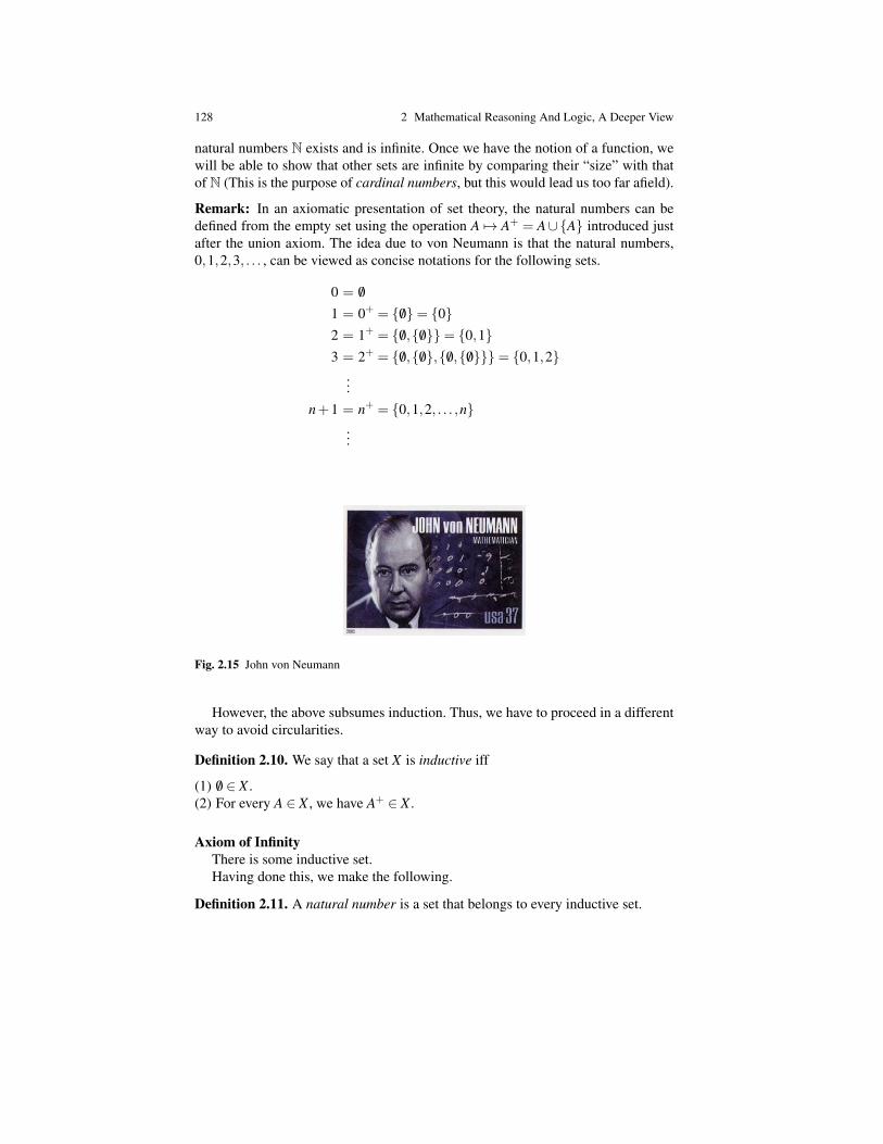
128 2 Mathematical Reasoning And Logic, A Deeper View
natural numbers N exists and is infinite. Once we have the notion of a function, wewill be able to show that other sets are infinite by comparing their “size” with thatof N (This is the purpose of cardinal numbers, but this would lead us too far afield).
Remark: In an axiomatic presentation of set theory, the natural numbers can bedefined from the empty set using the operation A 7→ A+ = A∪A introduced justafter the union axiom. The idea due to von Neumann is that the natural numbers,0,1,2,3, . . . , can be viewed as concise notations for the following sets.
0 = /01 = 0+ = /0= 02 = 1+ = /0, /0= 0,13 = 2+ = /0, /0, /0, /0= 0,1,2
...n+1 = n+ = 0,1,2, . . . ,n
...
Fig. 2.15 John von Neumann
However, the above subsumes induction. Thus, we have to proceed in a differentway to avoid circularities.
Definition 2.10. We say that a set X is inductive iff
(1) /0 ∈ X .(2) For every A ∈ X , we have A+ ∈ X .
Axiom of InfinityThere is some inductive set.Having done this, we make the following.
Definition 2.11. A natural number is a set that belongs to every inductive set.
2.12 Basics Concepts of Set Theory 129
Using the subset axioms, we can show that there is a set whose members areexactly the natural numbers. The argument is very similar to the one used to provethat arbitrary intersections exist. By the axiom of infinity, there is some inductiveset, say A. Now consider the property P(x) which asserts that x belongs to everyinductive set. By the subset axioms applied to P, there is a set, N, such that
x ∈ N iff x ∈ A and P(x)
and because A is inductive and P says that x belongs to every inductive set, the aboveis equivalent to
x ∈ N iff P(x);
that is, x ∈ N iff x belongs to every inductive set. Therefore, the set of all naturalnumbers N does exist. The set N is also denoted ω . We can now easily show thefollowing.
Theorem 2.4. The set N is inductive and it is a subset of every inductive set.
Proof . Recall that /0 belongs to every inductive set; so, /0 is a natural number (0).As N is the set of natural numbers, /0 (= 0) belongs to N. Secondly, if n ∈ N, thismeans that n belongs to every inductive set (n is a natural number), which impliesthat n+ = n+ 1 belongs to every inductive set, which means that n+ 1 is a naturalnumber, that is, n+ 1 ∈ N. Because N is the set of natural numbers and becauseevery natural number belongs to every inductive set, we conclude that N is a subsetof every inductive set. ut
It would be tempting to view N as the intersection of the family of inductivesets, but unfortunately this family is not a set; it is too “big” to be a set.
As a consequence of the above fact, we obtain the following.
Induction Principle for N: Any inductive subset of N is equal to N itself.Now, in our setting, 0 = /0 and n+ = n+1, so the above principle can be restated
as follows.
Induction Principle for N (Version 2): For any subset, S⊆N, if 0∈ S and n+1∈ Swhenever n ∈ S, then S = N.
We show how to rephrase this induction principle a little more conveniently interms of the notion of function in the next chapter.
Remarks:
1. We still don’t know what an infinite set is or, for that matter, that N is infinite.This is shown in the next chapter (see Corollary 3.12).
2. Zermelo–Fraenkel set theory (+ Choice) has three more axioms that we didnot discuss: The axiom of choice, the replacement axioms and the regularityaxiom. For our purposes, only the axiom of choice is needed and we introduceit in Chapter 3. Let us just say that the replacement axioms are needed to dealwith ordinals and cardinals and that the regularity axiom is needed to show that

130 2 Mathematical Reasoning And Logic, A Deeper View
every set is grounded. For more about these axioms, see Enderton [3], Chapter7. The regularity axiom also implies that no set can be a member of itself, aneventuality that is not ruled out by our current set of axioms.
As we said at the beginning of this section, set theory can be axiomatized infirst-order logic. To illustrate the generality and expressiveness of first-order logic,we conclude this section by stating the axioms of Zermelo–Fraenkel set theory (forshort, ZF) as first-order formulae. The language of Zermelo–Fraenkel set theoryconsists of the constant /0 (for the empty set), the equality symbol, and of the binarypredicate symbol ∈ for set membership. It is convenient to abbreviate ¬(x = y) asx 6= y and ¬(x ∈ y) as x /∈ y. The axioms are the equality axioms plus the followingseven axioms.
∀A∀B(∀x(x ∈ A≡ x ∈ B)⇒ A = B)
∀x(x /∈ /0)∀a∀b∃Z∀x(x ∈ Z ≡ (x = a∨ x = b))
∀X∃Y∀x(x ∈ Y ≡ ∃B(B ∈ X ∧ x ∈ B))
∀A∃Y∀X(X ∈ Y ≡ ∀z(z ∈ X ⇒ z ∈ A))
∀A∃X∀x(x ∈ X ≡ (x ∈ A)∧P)
∃X( /0 ∈ X ∧∀y(y ∈ X ⇒ y∪y ∈ X)),
where P is any first-order formula that does not contain X free.
• Axiom (1) is the extensionality axiom.• Axiom (2) is the empty set axiom.• Axiom (3) asserts the existence of a set Y whose only members are a and b. By
extensionality, this set is unique and it is denoted a,b. We also denote a,aby a.
• Axiom (4) asserts the existence of set Y which is the union of all the sets thatbelong to X . By extensionality, this set is unique and it is denoted
⋃X . When
X = A,B, we write⋃A,B= A∪B.
• Axiom (5) asserts the existence of set Y which is the set of all subsets of A (thepower set of A). By extensionality, this set is unique and it is denoted P(A) or2A.
• Axioms (6) are the subset axioms (or axioms of separation).• Axiom (7) is the infinity axiom, stated using the abbreviations introduced above.
For a comprehensive treatment of axiomatic theory (including the missing threeaxioms), see Enderton [3] and Suppes [20].
2.13 Summary
The main goal of this chapter is to describe precisely the logical rules used in mathe-matical reasoning and the notion of a mathematical proof. A brief introduction to set
2.13 Summary 131
theory is also provided. We decided to describe the rules of reasoning in a formal-ism known as a natural deduction system because the logical rules of such a systemmimic rather closely the informal rules that (nearly) everybody uses when construct-ing a proof in everyday life. Another advantage of natural deduction systems is thatit is very easy to present various versions of the rules involving negation and thus,to explain why the “proof-by-contradiction” proof rule or the “law of the excludedmiddle” allow for the derivation of “nonconstructive” proofs. This is a subtle pointoften not even touched in traditional presentations of logic. However, inasmuch asmost of our readers write computer programs and expect that their programs willnot just promise to give an answer but will actually produce results, we feel thatthey will grasp rather easily the difference between constructive and nonconstruc-tive proofs, and appreciate the latter, even if they are harder to find.
• We describe the syntax of propositional logic.• The proof rules for implication are defined in a natural deduction system
(Prawitz-style).• Deductions proceed from assumptions (or premises) using inference rules.• The process of discharging (or closing) a premise is explained. A proof is a
deduction in which all the premises have been discharged.• We explain how we can search for a proof using a combined bottom-up and
top-down process.• We propose another mechanism for decribing the process of discharging a
premise and this leads to a formulation of the rules in terms of sequents andto a Gentzen system.
• We introduce falsity ⊥ and negation ¬P as an abbrevation for P⇒⊥. We de-scribe the inference rules for conjunction, disjunction, and negation, in bothPrawitz style and Gentzen-sequent style natural deduction systems
• One of the rules for negation is the proof-by-contradiction rule (also known asRAA).
• We define intuitionistic and classical logic.• We introduce the notion of a constructive (or intuitionistic) proof and discuss
the two nonconstructive culprits: P∨¬P (the law of the excluded middle) and¬¬P⇒ P (double-negation rule).
• We show that P∨¬P and ¬¬P⇒ P are provable in classical logic• We clear up some potential confusion involving the various versions of the rules
regarding negation.
1. RAA is not a special case of ¬-introduction.2. RAA is not equivalent to ⊥-elimination; in fact, it implies it.3. Not all propositions of the form P∨¬P are provable in intuitionistic logic.
However, RAA holds in intuitionistic logic plus all propositions of the formP∨¬P.
4. We define double-negation elimination.
• We present the de Morgan laws and prove their validity in classical logic.• We present the proof-by-contrapositive rule and show that it is valid in classical
logic.

132 2 Mathematical Reasoning And Logic, A Deeper View
• We give some examples of proofs of “real” statements.• We give an example of a nonconstructive proof of the statement: there are two
irrational numbers, a and b, so that ab is rational.• We explain the truth-value semantics of propositional logic.• We define the truth tables for the propositional connectives• We define the notions of satisfiability, unsatisfiability, validity, and tautology.• We define the satisfiability problem and the validity problem (for classical
propositional logic).• We mention the NP-completeness of satisfiability.• We discuss soundness (or consistency) and completeness.• We state the soundness and completeness theorems for propositional classical
logic formulated in natural deduction.• We explain how to use counterexamples to prove that certain propositions are
not provable.• We give a brief introduction to Kripke semantics for propositional intuitionistic
logic.• We define Kripke models (based on a set of worlds).• We define validity in a Kripke model.• We state the the soundness and completeness theorems for propositional intu-
itionistic logic formulated in natural deduction.• We add first-order quantifiers (“for all” ∀ and “there exists” ∃) to the language
of propositional logic and define first-order logic.• We describe free and bound variables.• We give inference rules for the quantifiers in Prawitz-style and Gentzen sequent-
style natural deduction systems.• We explain the eigenvariable restriction in the ∀-introduction and ∃-elimination
rules.• We prove some “de Morgan”-type rules for the quantified formulae valid in
classical logic.• We discuss the nonconstructiveness of proofs of certain existential statements.• We explain briefly how classical logic can be translated into intuitionistic logic
(the Godel translation).• We define first-order theories and give the example of Peano arithmetic.• We revisit the decision problem and mention the undecidability of the decision
problem for first-order logic (Church’s theorem).• We discuss the notion of detours in proofs and the notion of proof normaliza-
tion.• We mention strong normalization.• We mention the correspondence between propositions and types and proofs and
typed λ -terms (the Curry–Howard isomorphism).• We mention Godel’s completeness theorem for first-order logic.• Again, we mention the use of counterexamples.• We mention Godel’s incompleteness theorem.• We present informally the axioms of Zermelo–Fraenkel set theory (ZF).

2.13 Problems 133
• We present Russell’s paradox, a warning against “self-referential” definitions ofsets.
• We define the empty set ( /0), the set a,b, whose elements are a and b, theunion A∪B, of two sets A and B, and the power set 2A, of A.
• We state carefully Zermelo’s subset axioms for defining the subset x ∈ A | Pof elements of a given set A satisfying a property P.
• Then, we define the intersection A∩B, and the relative complement A−B, oftwo sets A and B.
• We also define the union⋃
A and the intersection⋂
A, of a set of sets A.• We show that one should avoid sets that are “too big;” in particular, we prove
that there is no set of all sets.• We define the natural numbers “a la Von Neumann.”• We define inductive sets and state the axiom of infinity.• We show that the natural numbers form an inductive set N, and thus, obtain an
induction principle for N.• We summarize the axioms of Zermelo–Fraenkel set theory in first-order logic.
Problems
2.1. (a) Give a proof of the proposition P⇒ (Q⇒ P) in the system N ⇒m .
(b) Prove that if there are deduction trees of P⇒ Q and Q⇒ R from the set ofpremises Γ in the system N ⇒
m , then there is a deduction tree for P⇒ R from Γ inN ⇒
m .
2.2. Give a proof of the proposition (P⇒ Q)⇒ ((P⇒ (Q⇒ R))⇒ (P⇒ R)) inthe system N ⇒
m .
2.3. (a) Prove the “de Morgan” laws in classical logic:
¬(P∧Q)≡ ¬P∨¬Q
¬(P∨Q)≡ ¬P∧¬Q.
(b) Prove that ¬(P∨Q)≡ ¬P∧¬Q is also provable in intuitionistic logic.(c) Prove that the proposition (P∧¬Q)⇒¬(P⇒Q) is provable in intuitionistic
logic and ¬(P⇒ Q)⇒ (P∧¬Q) is provable in classical logic.
2.4. (a) Show that P⇒¬¬P is provable in intuitionistic logic.(b) Show that ¬¬¬P and ¬P are equivalent in intuitionistic logic.
2.5. Show that if we assume that all propositions of the form P∨¬P are provable,then the proof-by-contradiction rule can be established from the rules of intuitionis-tic logic.
2.6. Recall that an integer is even if it is divisible by 2, that is, if it can be writtenas 2k, where k ∈ Z. An integer is odd if it is not divisible by 2, that is, if it can bewritten as 2k+1, where k ∈ Z. Prove the following facts.
134 2 Mathematical Reasoning And Logic, A Deeper View
(a) The sum of even integers is even.(b) The sum of an even integer and of an odd integer is odd.(c) The sum of two odd integers is even.(d) The product of odd integers is odd.(e) The product of an even integer with any integer is even.
2.7. (a) Show that if we assume that all propositions of the form
P⇒ (Q⇒ R)
are axioms (where P,Q,R are arbitrary propositions), then every proposition is prov-able.
(b) Show that if P is provable (intuitionistically or classically), then Q⇒ P isalso provable for every proposition Q.
2.8. (a) Give intuitionistic proofs for the equivalences
P∨P≡ P
P∧P≡ P
P∨Q≡ Q∨P
P∧Q≡ Q∧P.
(b) Give intuitionistic proofs for the equivalences
P∧ (P∨Q)≡ P
P∨ (P∧Q)≡ P.
2.9. Give intuitionistic proofs for the propositions
P⇒ (Q⇒ (P∧Q))
(P⇒ Q)⇒ ((P⇒¬Q)⇒¬P)
(P⇒ R)⇒ ((Q⇒ R)⇒ ((P∨Q)⇒ R)).
2.10. Prove that the following equivalences are provable intuitionistically:
P∧ (P⇒ Q) ≡ P∧Q
Q∧ (P⇒ Q) ≡ Q(P⇒ (Q∧R)
)≡((P⇒ Q)∧ (P⇒ R)
).
2.11. Give intuitionistic proofs for
(P⇒ Q)⇒¬¬(¬P∨Q)
¬¬(¬¬P⇒ P).
2.12. Give an intuitionistic proof for ¬¬(P∨¬P).

2.13 Problems 135
2.13. Give intuitionistic proofs for the propositions
(P∨¬P)⇒ (¬¬P⇒ P) and (¬¬P⇒ P)⇒ (P∨¬P).
Hint. For the second implication, you may want to use Problem 2.12.
2.14. Give intuitionistic proofs for the propositions
(P⇒ Q)⇒¬¬(¬P∨Q) and (¬P⇒ Q)⇒¬¬(P∨Q).
2.15. (1) Prove that every deduction (in N ⇒,∧,∨,⊥c or N ⇒,∧,∨,⊥
i ) of a proposition Pfrom any set of premises Γ ,
Γ
D
P
can be converted to a deduction of P from the set of premises Γ ∪∆ , where ∆ is anyset of propositions (not necessarily disjoint from Γ ):
Γ ∪∆
D ′
P(2) Consider the proof system obtained by changing the following rules of the
proof system N ⇒,∧,∨,⊥c given in Definition 2.3:
⇒-elimination rule:
Γ
D1
P⇒ Q
∆
D2
P
Q∧-introduction rule:
Γ
D1
P
∆
D2
Q
P∧Q∨-elimination rule:
Γ
D1
P∨Q
∆ ,Px
D2
R
Λ ,Qy
D3
Rx,y
R¬-elimination rule:
136 2 Mathematical Reasoning And Logic, A Deeper View
Γ
D1
¬P
∆
D2
P
⊥to the following rules using the same set of premises Γ :⇒-elimination rule′:
Γ
D1
P⇒ Q
Γ
D2
P
Q∧-introduction rule′:
Γ
D1
P
Γ
D2
Q
P∧Q∨-elimination rule′:
Γ
D1
P∨Q
Γ ,Px
D2
R
Γ ,Qy
D3
Rx,y
R¬-elimination rule′:
Γ
D1
¬P
Γ
D2
P
⊥and call the resulting proof system N ′
c⇒,∧,∨,⊥.
Prove that every deduction in N ′c⇒,∧,∨,⊥ of a proposition P from a set of
premises Γ can be converted to a deduction of P from Γ in N ′c⇒,∧,∨,⊥.
Hint. Use induction on deduction trees and part (1) of the problem.Conclude from the above that the same set of propositions is provable in the
systems N ⇒,∧,∨,⊥c and N ′
c⇒,∧,∨,⊥ and similarly for N ⇒,∧,∨,⊥
i and N ′i⇒,∧,∨,⊥,
the systems obtained by dropping the proof-by-contradiction rule.
2.16. Prove that the following version of the ∨-elimination rule formulated inGentzen-sequent style is a consequence of the rules of intuitionistic logic:
Γ ,x : P→ R Γ ,y : Q→ RΓ ,z : P∨Q→ R
2.13 Problems 137
Conversely, if we assume that the above rule holds, then prove that the ∨-elimination rule
Γ → P∨Q Γ ,x : P→ R Γ ,y : Q→ RΓ → R
(∨-elim)
follows from the rules of intuitionistic logic (of course, excluding the ∨-eliminationrule).
2.17. (1) Prove that every deduction (in the proof system N ⇒,∧,∨,⊥,∀,∃c or the proof
system N ⇒,∧,∨,⊥,∀,∃i ) of a formula P from any set of premises Γ ,
Γ
D
P
can be converted to a deduction of P from the set of premises Γ ∪∆ , where ∆ is anyset of formulae (not necessarily disjoint from Γ ) such that all the variable free in Γ
are distinct from all the eigenvariables occurring in the original deduction:
Γ ∪∆
D ′
P(2) Let Γ = P1, . . . ,Pn be a set of first-order formulae. If t1, . . . , tm is the set
of all variables occurring free in the formulae in Γ , we denote by Γ [τ1/t1, . . . ,τm/tm]the set of substituted formulae
P1[τ1/t1, . . . ,τm/tm], . . . ,Pm[τ1/t1, . . . ,τm/tm],
where τ1, . . . ,τm are any terms such that no capture takes place when the substitu-tions are made.
Given any deduction of a formula P from a set of premises Γ (in the proof systemN ⇒,∧,∨,⊥,∀,∃
c or the proof system N ⇒,∧,∨,⊥,∀,∃i ), if t1, . . . , tm is the set of all the
variables occurring free in the formulae in Γ , then prove that there is a deductionof P[u1/t1, . . . ,um/tm] from Γ [u1/t1, . . . ,um/tm], where u1, . . . ,um is a set of vari-ables not occurring free or bound in any of the propositions in Γ or in P (e.g., a setof “fresh” variables).Hint. Use induction on deduction trees.
(3) Prove that every deduction (in the proof system N ⇒,∧,∨,⊥,∀,∃c or the proof
system N ⇒,∧,∨,⊥,∀,∃i ) using the ∃-elimination rule
Γ
D1
∃tP
∆ ,P[u/t]x
D2
Cx
C
(with the usual restriction on u) can be converted to a deduction using the followingversion of the ∃-elimination rule.
138 2 Mathematical Reasoning And Logic, A Deeper View
Γ
D1
∃tP
Γ ,P[u/t]x
D2
Cx
C
where u is a variable that does not occur free in any of the propositions in Γ , ∃tP,or C.Hint. Use induction on deduction trees and parts (1) and (2) of this problem.
2.18. (a) Give intuitionistic proofs for the distributivity of ∧ over ∨ and of ∨ over∧:
P∧ (Q∨R)≡ (P∧Q)∨ (P∧R)
P∨ (Q∧R)≡ (P∨Q)∧ (P∨R).
(b) Give intuitionistic proofs for the associativity of ∧ and ∨:
P∧ (Q∧R)≡ (P∧Q)∧R
P∨ (Q∨R)≡ (P∨Q)∨R.
2.19. Recall that in Problem 2.1 we proved that if P⇒ Q and Q⇒ R are provable,then P⇒ R is provable. Deduce from this fact that if P ≡ Q and Q ≡ R hold, thenP≡ R holds (intuitionistically or classically).
Prove that if P ≡ Q holds then Q ≡ P holds (intuitionistically or classically).Finally, check that P≡ P holds (intuitionistically or classically).
2.20. Prove (intuitionistically or classically) that if P1⇒ Q1 and P2⇒ Q2 then
1. (P1∧P2)⇒ (Q1∧Q2)2. (P1∨P2)⇒ (Q1∨Q2).
(b) Prove (intuitionistically or classically) that if Q1⇒ P1 and P2⇒ Q2 then
1. (P1⇒ P2)⇒ (Q1⇒ Q2)2. ¬P1⇒¬Q1.
(c) Prove (intuitionistically or classically) that if P⇒ Q, then
1. ∀tP⇒∀tQ2. ∃tP⇒∃tQ.
(d) Prove (intuitionistically or classically) that if P1 ≡ Q1 and P2 ≡ Q2 then
1. (P1∧P2)≡ (Q1∧Q2)2. (P1∨P2)≡ (Q1∨Q2)3. (P1⇒ P2)≡ (Q1⇒ Q2)4. ¬P1 ≡ ¬Q15. ∀tP1 ≡ ∀tQ16. ∃tP1 ≡ ∃tQ1.
2.13 Problems 139
2.21. Show that the following are provable in classical first-order logic:
¬∀tP≡ ∃t¬P
¬∃tP≡ ∀t¬P
∀t(P∧Q)≡ ∀tP∧∀tQ∃t(P∨Q)≡ ∃tP∨∃tQ.
(b) Moreover, show that the propositions ∃t(P∧Q)⇒∃tP∧∃tQ and∀tP∨∀tQ⇒∀t(P∨Q) are provable in intuitionistic first-order logic (and thus, alsoin classical first-order logic).
(c) Prove intuitionistically that
∃x∀yP⇒∀y∃xP.
Give an informal argument to the effect that the converse, ∀y∃xP⇒ ∃x∀yP, isnot provable, even classically.
2.22. (a) Assume that Q is a formula that does not contain the variable t (free orbound). Give a classical proof of
∀t(P∨Q)⇒ (∀tP∨Q).
(b) If P is a proposition, write P(x) for P[x/t] and P(y) for P[y/t], where x and y aredistinct variables that do not occur in the orginal proposition P. Give an intuitionisticproof for
¬∀x∃y(¬P(x)∧P(y)).
(c) Give a classical proof for
∃x∀y(P(x)∨¬P(y)).
Hint. Negate the above, then use some identities we’ve shown (such as de Morgan)and reduce the problem to part (b).
2.23. (a) Let X = Xi | 1 ≤ i ≤ n be a finite family of sets. Prove that if Xi+1 ⊆ Xifor all i, with 1≤ i≤ n−1, then ⋂
X = Xn.
Prove that if Xi ⊆ Xi+1 for all i, with 1≤ i≤ n−1, then⋃X = Xn.
(b) Recall that N+ =N−0= 1,2,3, . . . ,n, . . .. Give an example of an infinitefamily of sets, X = Xi | i ∈ N+, such that
1. Xi+1 ⊆ Xi for all i≥ 1.2. Xi is infinite for every i≥ 1.
140 2 Mathematical Reasoning And Logic, A Deeper View
3.⋂
X has a single element.
(c) Give an example of an infinite family of sets, X = Xi | i ∈ N+, such that
1. Xi+1 ⊆ Xi for all i≥ 1.2. Xi is infinite for every i≥ 1.3.⋂
X = /0.
2.24. Prove that the following propositions are provable intuitionistically:
(P⇒¬P)≡ ¬P, (¬P⇒ P)≡ ¬¬P.
Use these to conlude that if the equivalence P ≡ ¬P is provable intuitionistically,then every proposition is provable (intuitionistically).
2.25. (1) Prove that if we assume that all propositions of the form,
((P⇒ Q)⇒ P)⇒ P,
are axioms (Peirce’s law), then ¬¬P⇒ P becomes provable in intuitionistic logic.Thus, another way to get classical logic from intuitionistic logic is to add Peirce’slaw to intuitionistic logic.Hint. Pick Q in a suitable way and use Problem 2.24.
(2) Prove ((P⇒ Q)⇒ P)⇒ P in classical logic.Hint. Use the de Morgan laws.
2.26. Let A be any nonempty set. Prove that the definition
X = a ∈ A | a /∈ X
yields a “set,” X , such that X is empty iff X is nonempty and therefore does notdefine a set, after all.
2.27. Prove the following fact: if
Γ
D1
P∨Qand
Γ ,R
D2
Q
are deduction trees provable intuitionistically, then there is a deduction tree
Γ ,P⇒ R
D
Q
for Q from the premises in Γ ∪P⇒ S.
2.28. Recall that the constant > stands for true. So, we add to our proof systems(intuitionistic and classical) all axioms of the form
2.13 Problems 141
k1︷ ︸︸ ︷P1, . . . ,P1, . . . ,
ki︷ ︸︸ ︷Pi, . . . ,Pi, . . . ,
kn︷ ︸︸ ︷Pn, . . . ,Pn
>where ki ≥ 1 and n≥ 0; note that n = 0 is allowed, which amounts to the one-nodetree, >.
(a) Prove that the following equivalences hold intuitionistically.
P ∨>≡>P ∧>≡ P.
Prove that if P is intuitionistically (or classically) provable, then P ≡ > is alsoprovable intuitionistically (or classically). In particular, in classical logic,P∨¬P≡>. Also prove that
P ∨ ⊥≡ P
P ∧ ⊥≡⊥
hold intuitionistically.(b) In the rest of this problem, we are dealing only with classical logic. The
connective exclusive or, denoted ⊕, is defined by
P⊕Q≡ (P∧¬Q)∨ (¬P∧Q).
In solving the following questions, you will find that constructing proofs using therules of classical logic is very tedious because these proofs are very long. Instead,use some identities from previous problems.
Prove the equivalence¬P≡ P⊕>.
(c) Prove that
P⊕P≡⊥P⊕Q≡ Q⊕P
(P⊕Q)⊕R≡ P⊕ (Q⊕R).
(d) Prove the equivalence
P∨Q≡ (P∧Q)⊕ (P⊕Q).
2.29. Give a classical proof of
¬(P⇒¬Q)⇒ (P∧Q).
2.30. (a) Prove that the rule
142 2 Mathematical Reasoning And Logic, A Deeper View
Γ
D1
P⇒ Q
∆
D2
¬Q
¬P
can be derived from the other rules of intuitionistic logic.(b) Give an intuitionistic proof of ¬P from Γ = ¬(¬P∨Q),P⇒ Q or equiva-
lently, an intuitionistic proof of(¬(¬P∨Q)∧ (P⇒ Q)
)⇒¬P.
2.31. (a) Give intuitionistic proofs for the equivalences
∃x∃yP≡ ∃y∃xP and ∀x∀yP≡ ∀y∀xP.
(b) Give intuitionistic proofs for
(∀tP∧Q)⇒∀t(P∧Q) and ∀t(P∧Q)⇒ (∀tP∧Q),
where t does not occur (free or bound) in Q.(c) Give intuitionistic proofs for
(∃tP∨Q)⇒∃t(P∨Q) and ∃t(P∨Q)⇒ (∃tP∨Q),
where t does not occur (free or bound) in Q.
2.32. An integer, n ∈ Z, is divisible by 3 iff n = 3k, for some k ∈ Z. Thus (by thedivision theorem), an integer, n ∈ Z, is not divisible by 3 iff it is of the form n =3k+1,3k+2, for some k ∈ Z (you don’t have to prove this).
Prove that for any integer, n ∈ Z, if n2 is divisible by 3, then n is divisible by 3.
Hint. Prove the contrapositive. If n of the form n = 3k+1,3k+2, then so is n2 (fora different k).
2.33. Use Problem 2.32 to prove that√
3 is irrational, that is,√
3 can’t be written as√3 = p/q, with p,q ∈ Z and q 6= 0.
2.34. Give an intuitionistic proof of the proposition((P⇒ R)∧ (Q⇒ R)
)≡((P∨Q)⇒ R
).
2.35. Give an intuitionistic proof of the proposition((P∧Q)⇒ R
)≡(P⇒ (Q⇒ R)
).
2.36. (a) Give an intuitionistic proof of the proposition(P∧Q)⇒ (P∨Q).
2.13 Problems 143
(b) Prove that the proposition (P∨Q)⇒ (P∧Q) is not valid, where P,Q, arepropositional symbols.
(c) Prove that the proposition (P∨Q)⇒ (P∧Q) is not provable in general andthat if we assume that all propositions of the form (P∨Q)⇒ (P∧Q) are axioms,then every proposition becomes provable intuitionistically.
2.37. Give the details of the proof of Proposition 2.8; namely, if a proposition P isprovable in the system N ⇒,∧,∨,⊥
c (or N G⇒,∧,∨,⊥c ), then it is valid (according to the
truth value semantics).
2.38. Give the details of the proof of Theorem 2.9; namely, if a proposition P isprovable in the system N ⇒,∧,∨,⊥
i (or N G⇒,∧,∨,⊥i ), then it is valid in every Kripke
model; that is, it is intuitionistically valid.
2.39. Prove that b = log2 9 is irrational. Then, prove that a =√
2 and b = log2 9 aretwo irrational numbers such that ab is rational.
2.40. (1) Prove that if ∀x¬(P∧Q) can be deduced intuitionistically from a set ofpremises Γ , then ∀x(P⇒¬Q) and ∀x(Q⇒¬P) can also be deduced intuitionisti-cally from Γ .
(2) Prove that if ∀x(P ∨ Q) can be deduced intuitionistically from a set ofpremises Γ , then ∀x(¬P⇒ Q) and ∀x(¬Q⇒ P) can also be deduced intuitionis-tically from Γ .
Conclude that if∀x(P∨Q) and ∀x¬(P∧Q)
can be deduced intuitionistically from a set of premises Γ , then
∀x(P≡ ¬Q) and ∀x(Q≡ ¬P)
can also be deduced intuitionistically from Γ .(3) Prove that if ∀x(P ⇒ Q) can be deduced intuitionistically from a set of
premises Γ , then ∀x(¬Q⇒¬P) can also be deduced intuitionistically from Γ . Usethis to prove that if
∀x(P≡ ¬Q) and ∀x(Q≡ ¬P)
can be deduced intuitionistically from a set of premises Γ , then ∀x(¬¬P≡ P) and∀x(¬¬Q≡ Q) can be deduced intuitionistically from Γ .
2.41. Prove that the formula,∀xeven(2∗ x),
is provable in Peano arithmetic. Prove that
even(2∗ (n+1)∗ (n+3)),
is provable in Peano arithmetic for any natural number n.
2.42. A first-order formula A is said to be in prenex-form if either
144 2 Mathematical Reasoning And Logic, A Deeper View
(1) A is a quantifier-free formula.(2) A = ∀tB or A = ∃tB, where B is in prenex-form.
In other words, a formula is in prenex form iff it is of the form
Q1t1Q2t2 · · ·Qmtm P,
where P is quantifier-free and where Q1Q2 · · ·Qm is a string of quantifiers, Qi ∈∀,∃.
Prove that every first-order formula A is classically equivalent to a formula B inprenex form.
2.43. Even though natural deduction proof systems for classical propositional logicare complete (with respect to the truth value semantics), they are not adequate fordesigning algorithms searching for proofs (because of the amount of nondetermin-ism involved).
Gentzen designed a different kind of proof system using sequents (later refinedby Kleene, Smullyan, and others) that is far better suited for the design of automatedtheorem provers. Using such a proof system (a sequent calculus), it is relatively easyto design a procedure that terminates for all input propositions P and either certifiesthat P is (classically) valid or else returns some (or all) falsifying truth assignment(s)for P. In fact, if P is valid, the tree returned by the algorithm can be viewed as a proofof P in this proof system.
For this miniproject, we describe a Gentzen sequent-calculus G′ for propositionallogic that lends itself well to the implementation of algorithms searching for proofsor falsifying truth assignments of propositions.
Such algorithms build trees whose nodes are labeled with pairs of sets calledsequents. A sequent is a pair of sets of propositions denoted by
P1, . . . ,Pm→ Q1, . . . ,Qn,
with m,n≥ 0. Symbolically, a sequent is usally denoted Γ → ∆ , where Γ and ∆ aretwo finite sets of propositions (not necessarily disjoint).
For example,
→ P⇒ (Q⇒ P), P∨Q→, P,Q→ P∧Q
are sequents. The sequent→, where both Γ = ∆ = /0 corresponds to falsity.The choice of the symbol→ to separate the two sets of propositions Γ and ∆ is
commonly used and was introduced by Gentzen but there is nothing special aboutit. If you don’t like it, you may replace it by any symbol of your choice as long asthat symbol does not clash with the logical connectives (⇒,∧,∨,¬). For example,you could denote a sequent
P1, . . . ,Pm;Q1, . . . ,Qn,
using the semicolon as a separator.
2.13 Problems 145
Given a truth assignment v to the propositional letters in the propositions Pi andQ j, we say that v satisfies the sequent, P1, . . . ,Pm→ Q1, . . . ,Qn, iff
v((P1∧·· ·∧Pm)⇒ (Q1∨·· ·∨Qn)) = true,
or equivalently, v falsifies the sequent, P1, . . . ,Pm→ Q1, . . . ,Qn, iff
v(P1∧·· ·∧Pm∧¬Q1∧·· ·∧¬Qn) = true,
iffv(Pi) = true, 1≤ i≤ m and v(Q j) = false, 1≤ j ≤ n.
A sequent is valid iff it is satisfied by all truth assignments iff it cannot be falsified.Note that a sequent P1, . . . ,Pm→ Q1, . . . ,Qn can be falsified iff some truth as-
signment satisfies all of P1, . . . ,Pm and falsifies all of Q1, . . . ,Qn. In particular,if P1, . . . ,Pm and Q1, . . . ,Qn have some common proposition (they have anonempty intersection), then the sequent, P1, . . . ,Pm→ Q1, . . . ,Qn, is valid. On theother hand if all the Pis and Q js are propositional letters and P1, . . . ,Pm andQ1, . . . ,Qn are disjoint (they have no symbol in common), then the sequent,P1, . . . ,Pm→ Q1, . . . ,Qn, is falsified by the truth assignment v where v(Pi) = true,for i = 1, . . .m and v(Q j) = false, for j = 1, . . . ,n.
The main idea behind the design of the proof system G′ is to systematically tryto falsify a sequent. If such an attempt fails, the sequent is valid and a proof tree isfound. Otherwise, all falsifying truth assignments are returned. In some sense
failure to falsify is success (in finding a proof).
The rules of G′ are designed so that the conclusion of a rule is falsified by a truthassignment v iff its single premise of one of its two premises is falsified by v. Thus,these rules can be viewed as two-way rules that can either be read bottom-up ortop-down.
Here are the axioms and the rules of the sequent calculus G′:Axioms: Γ ,P→ P,∆Inference rules:
146 2 Mathematical Reasoning And Logic, A Deeper View
Γ ,P,Q,∆ →Λ
Γ ,P∧Q,∆ →Λ∧: left
Γ → ∆ ,P,Λ Γ → ∆ ,Q,Λ
Γ → ∆ ,P∧Q,Λ∧: right
Γ ,P,∆ →Λ Γ ,Q,∆ →Λ
Γ ,P∨Q,∆ →Λ∨: left
Γ → ∆ ,P,Q,Λ
Γ → ∆ ,P∨Q,Λ∨: right
Γ ,∆ → P,Λ Q,Γ ,∆ →Λ
Γ ,P⇒ Q,∆ →Λ⇒: left
P,Γ → Q,∆ ,Λ
Γ → ∆ ,P⇒ Q,Λ⇒: right
Γ ,∆ → P,ΛΓ ,¬P,∆ →Λ
¬: leftP,Γ → ∆ ,Λ
Γ → ∆ ,¬P,Λ¬: right
where Γ ,∆ ,Λ are any finite sets of propositions, possibly the empty set.A deduction tree is either a one-node tree labeled with a sequent or a tree con-
structed according to the rules of system G′. A proof tree (or proof ) is a deductiontree whose leaves are all axioms. A proof tree for a proposition P is a proof tree forthe sequent→ P (with an empty left-hand side).
For example,P,Q→ P
is a proof tree.Here is a proof tree for (P⇒ Q)⇒ (¬Q⇒¬P):
P,¬Q→ P
¬Q→¬P,P
→ P,(¬Q⇒¬P)
Q→ Q,¬P
¬Q,Q→¬P
Q→ (¬Q⇒¬P)
(P⇒ Q)→ (¬Q⇒¬P)
→ (P⇒ Q)⇒ (¬Q⇒¬P)
The following is a deduction tree but not a proof tree,
P,R→ P
R→¬P,P
→ P,(R⇒¬P)
R,Q,P→R,Q→¬P
Q→ (R⇒¬P)
(P⇒ Q)→ (R⇒¬P)
→ (P⇒ Q)⇒ (R⇒¬P)
because its rightmost leaf, R,Q,P→, is falsified by the truth assignmentv(P) = v(Q) = v(R) = true, which also falsifies (P⇒ Q)⇒ (R⇒¬P).
Let us call a sequent P1, . . . ,Pm→ Q1, . . . ,Qn finished if either it is an axiom(Pi = Q j for some i and some j) or all the propositions Pi and Q j are atomic
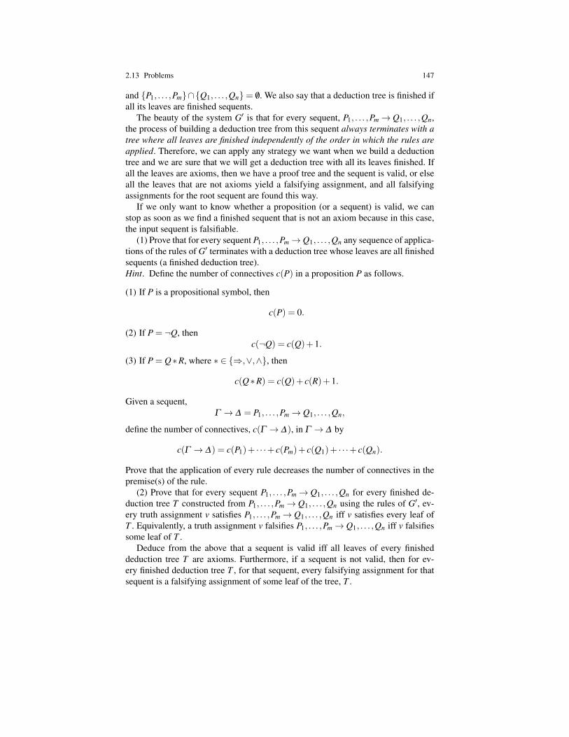
2.13 Problems 147
and P1, . . . ,Pm∩Q1, . . . ,Qn= /0. We also say that a deduction tree is finished ifall its leaves are finished sequents.
The beauty of the system G′ is that for every sequent, P1, . . . ,Pm→ Q1, . . . ,Qn,the process of building a deduction tree from this sequent always terminates with atree where all leaves are finished independently of the order in which the rules areapplied. Therefore, we can apply any strategy we want when we build a deductiontree and we are sure that we will get a deduction tree with all its leaves finished. Ifall the leaves are axioms, then we have a proof tree and the sequent is valid, or elseall the leaves that are not axioms yield a falsifying assignment, and all falsifyingassignments for the root sequent are found this way.
If we only want to know whether a proposition (or a sequent) is valid, we canstop as soon as we find a finished sequent that is not an axiom because in this case,the input sequent is falsifiable.
(1) Prove that for every sequent P1, . . . ,Pm→ Q1, . . . ,Qn any sequence of applica-tions of the rules of G′ terminates with a deduction tree whose leaves are all finishedsequents (a finished deduction tree).Hint. Define the number of connectives c(P) in a proposition P as follows.
(1) If P is a propositional symbol, then
c(P) = 0.
(2) If P = ¬Q, thenc(¬Q) = c(Q)+1.
(3) If P = Q∗R, where ∗ ∈ ⇒,∨,∧, then
c(Q∗R) = c(Q)+ c(R)+1.
Given a sequent,Γ → ∆ = P1, . . . ,Pm→ Q1, . . . ,Qn,
define the number of connectives, c(Γ → ∆), in Γ → ∆ by
c(Γ → ∆) = c(P1)+ · · ·+ c(Pm)+ c(Q1)+ · · ·+ c(Qn).
Prove that the application of every rule decreases the number of connectives in thepremise(s) of the rule.
(2) Prove that for every sequent P1, . . . ,Pm→ Q1, . . . ,Qn for every finished de-duction tree T constructed from P1, . . . ,Pm→ Q1, . . . ,Qn using the rules of G′, ev-ery truth assignment v satisfies P1, . . . ,Pm→ Q1, . . . ,Qn iff v satisfies every leaf ofT . Equivalently, a truth assignment v falsifies P1, . . . ,Pm→ Q1, . . . ,Qn iff v falsifiessome leaf of T .
Deduce from the above that a sequent is valid iff all leaves of every finisheddeduction tree T are axioms. Furthermore, if a sequent is not valid, then for ev-ery finished deduction tree T , for that sequent, every falsifying assignment for thatsequent is a falsifying assignment of some leaf of the tree, T .
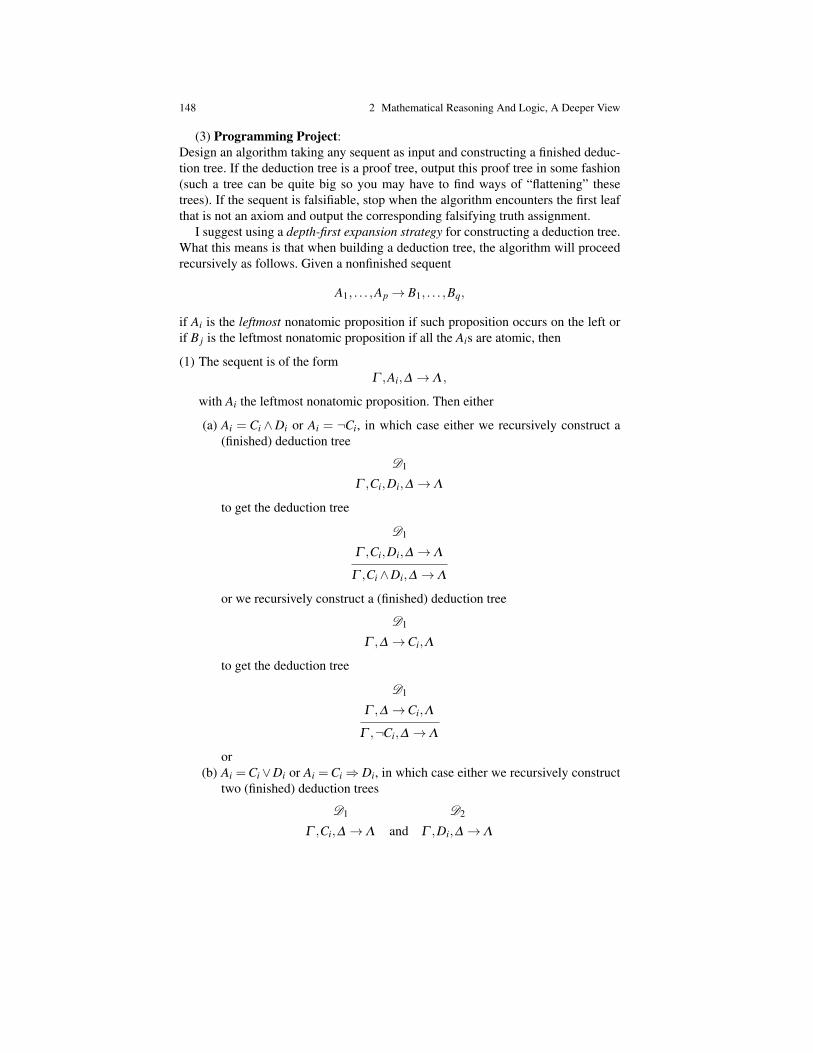
148 2 Mathematical Reasoning And Logic, A Deeper View
(3) Programming Project:Design an algorithm taking any sequent as input and constructing a finished deduc-tion tree. If the deduction tree is a proof tree, output this proof tree in some fashion(such a tree can be quite big so you may have to find ways of “flattening” thesetrees). If the sequent is falsifiable, stop when the algorithm encounters the first leafthat is not an axiom and output the corresponding falsifying truth assignment.
I suggest using a depth-first expansion strategy for constructing a deduction tree.What this means is that when building a deduction tree, the algorithm will proceedrecursively as follows. Given a nonfinished sequent
A1, . . . ,Ap→ B1, . . . ,Bq,
if Ai is the leftmost nonatomic proposition if such proposition occurs on the left orif B j is the leftmost nonatomic proposition if all the Ais are atomic, then
(1) The sequent is of the formΓ ,Ai,∆ →Λ ,
with Ai the leftmost nonatomic proposition. Then either
(a) Ai = Ci ∧Di or Ai = ¬Ci, in which case either we recursively construct a(finished) deduction tree
D1
Γ ,Ci,Di,∆ →Λ
to get the deduction tree
D1
Γ ,Ci,Di,∆ →Λ
Γ ,Ci∧Di,∆ →Λ
or we recursively construct a (finished) deduction tree
D1
Γ ,∆ →Ci,Λ
to get the deduction tree
D1
Γ ,∆ →Ci,Λ
Γ ,¬Ci,∆ →Λ
or(b) Ai =Ci∨Di or Ai =Ci⇒ Di, in which case either we recursively construct
two (finished) deduction trees
D1
Γ ,Ci,∆ →Λ and
D2
Γ ,Di,∆ →Λ

2.13 Problems 149
to get the deduction tree
D1
Γ ,Ci,∆ →Λ
D2
Γ ,Di,∆ →Λ
Γ ,Ci∨Di,∆ →Λ
or we recursively construct two (finished) deduction trees
D1
Γ ,∆ →Ci,Λ and
D2
Di,Γ ,∆ →Λ
to get the deduction tree
D1
Γ ,∆ →Ci,Λ
D2
Di,Γ ,∆ →Λ
Γ ,Ci⇒ Di,∆ →Λ
(2) The nonfinished sequent is of the form
Γ → ∆ ,B j,Λ ,
with B j the leftmost nonatomic proposition. Then either
(a) B j =C j ∨D j or B j =C j⇒D j, or B j = ¬C j, in which case either we recur-sively construct a (finished) deduction tree
D1
Γ → ∆ ,C j,D j,Λ
to get the deduction tree
D1
Γ → ∆ ,C j,D j,Λ
Γ → ∆ ,C j ∨D j,Λ
or we recursively construct a (finished) deduction tree
D1
C j,Γ → D j,∆ ,Λ
to get the deduction tree
D1
C j,Γ → D j,∆ ,Λ
Γ → ∆ ,C j⇒ D j,Λ
or we recursively construct a (finished) deduction tree
D1
C j,Γ → ∆ ,Λ
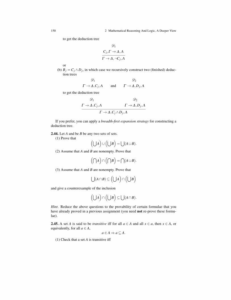
150 2 Mathematical Reasoning And Logic, A Deeper View
to get the deduction tree
D1
C j,Γ → ∆ ,Λ
Γ → ∆ ,¬C j,Λ
or(b) B j =C j ∧D j, in which case we recursively construct two (finished) deduc-
tion trees
D1
Γ → ∆ ,C j,Λ and
D2
Γ → ∆ ,D j,Λ
to get the deduction tree
D1
Γ → ∆ ,C j,Λ
D2
Γ → ∆ ,D j,Λ
Γ → ∆ ,C j ∧D j,Λ
If you prefer, you can apply a breadth-first expansion strategy for constructing adeduction tree.
2.44. Let A and be B be any two sets of sets.(1) Prove that (⋃
A)∪(⋃
B)=⋃(A∪B).
(2) Assume that A and B are nonempty. Prove that(⋂A)∩(⋂
B)=⋂(A∪B).
(3) Assume that A and B are nonempty. Prove that⋃(A∩B)⊆
(⋃A)∩(⋃
B)
and give a counterexample of the inclusion(⋃A)∩(⋃
B)⊆⋃(A∩B).
Hint. Reduce the above questions to the provability of certain formulae that youhave already proved in a previous assignment (you need not re-prove these formu-lae).
2.45. A set A is said to be transitive iff for all a ∈ A and all x ∈ a, then x ∈ A, orequivalently, for all a ∈ A,
a ∈ A⇒ a⊆ A.
(1) Check that a set A is transitive iff

References 151⋃A⊆ A
iffA⊆ 2A.
(2) Recall the definition of the von Neumann successor of a set A given by
A+ = A∪A.
Prove that if A is a transitive set, then⋃(A+) = A.
(3) Recall the von Neumann definition of the natural numbers. Check that forevery natural number m
m ∈ m+ and m⊆ m+.
Prove that every natural number is a transitive set.Hint. Use induction.
(4) Prove that for any two von Neumann natural numbers m and n, if m+ = n+,then m = n.
(5) Prove that the set, N, of natural numbers is a transitive set.Hint. Use induction.
References
1. Peter B. Andrews. An Introduction to Mathematical Logic and Type Theory: To truth ThroughProof. New York: Academic Press, 1986.
2. H.B. Curry and R. Feys. Combinatory Logic, Vol. I. Studies in Logic. Amsterdam: North-Holland, third edition, 1974.
3. Herbert B. Enderton. Elements of Set Theory. New York: Academic Press, first edition, 1977.4. Jean H. Gallier. Logic for Computer Science. New York: Harper and Row, 1986.5. Jean Gallier. Constructive logics. Part I: A tutorial on proof systems and typed λ -calculi.
Theoretical Computer Science, 110(2):249–339, 1993.6. Jean Gallier. On the Correspondence Between Proofs and λ -Terms. In Philippe de Groote,
editor, Cahiers Du Centre de Logique, Vol. 8, pages 55–138. Louvain-La-Neuve: Academia,1995.
7. G. Gentzen. Investigations into logical deduction. In M.E. Szabo, editor, The CollectedPapers of Gerhard Gentzen. Amsterdam: North-Holland, 1969.
8. J.-Y. Girard, Y. Lafont, and P. Taylor. Proofs and Types, volume 7 of Cambridge Tracts inTheoretical Computer Science. Cambridge, UK: Cambridge University Press, 1989.
9. Jean-Yves Girard. Linear logic. Theoretical Computer Science, 50:1–102, 1987.10. Timothy Gowers. Mathematics: A Very Short Introduction. Oxford, UK: Oxford University
Press, first edition, 2002.11. Paul R. Halmos. Naive Set Theory. Undergraduate Text in Mathematics. New York: Springer
Verlag, first edition, 1974.12. John E. Hopcroft, Rajeev Motwani, and Jeffrey D. Ullman. Introduction to Automata, Lan-
guages and Computation. Reading, MA: Addison Wesley, third edition, 2006.
152 2 Mathematical Reasoning And Logic, A Deeper View
13. W. A. Howard. The formulae-as-types notion of construction. In J. P. Seldin and J. R. Hindley,editors, To H. B. Curry: Essays on Combinatory Logic, Lambda Calculus and Formalism,pages 479–490. London: Academic Press, 1980. Reprint of manuscript first published in1969.
14. Michael Huth and Mark Ryan. Logic in Computer Science. Modelling and reasonning aboutsystems. Cambridge, UK: Cambridge University Press, 2000.
15. S. Kleene. Introduction to Metamathematics. Amsterdam: North-Holland, seventh edition,1952.
16. Harry Lewis and Christos H. Papadimitriou. Elements of the Theory of Computation. Engle-wood Cliffs, NJ: Prentice-Hall, second edition, 1997.
17. D. Prawitz. Natural Deduction, A Proof-Theoretical Study. Stockholm: Almquist & Wiksell,1965.
18. D. Prawitz. Ideas and results in proof theory. In J.E. Fenstad, editor, Proc. 2nd Scand. Log.Symp., pages 235–307. New York: North-Holland, 1971.
19. R. Statman. Intuitionistic propositional logic is polynomial-space complete. TheoreticalComputer Science, 9(1):67–72, 1979.
20. Patrick Suppes. Axiomatic Set Theory. New York: Dover, first edition, 1972.21. G. Takeuti. Proof Theory, volume 81 of Studies in Logic. Amsterdam: North-Holland, 1975.22. A.S. Troelstra and H. Schwichtenberg. Basic Proof Theory, volume 43 of Cambridge Tracts
in Theoretical Computer Science. Cambridge, UK: Cambridge University Press, 1996.23. D. van Dalen. Logic and Structure. New York: Universitext. Springer Verlag, second edition,
1980.
Chapter 3Relations, Functions, Partial Functions,Equivalence Relations
3.1 What is a Function?
We use functions all the time in mathematics and in computer science. But, whatexactly is a function?
Roughly speaking, a function f is a rule or mechanism that takes input values insome input domain, say X , and produces output values in some output domain, sayY , in such a way that to each input x ∈ X corresponds a unique output value y ∈ Y ,denoted f (x). We usually write y = f (x), or better, x 7→ f (x).
Often, functions are defined by some sort of closed expression (a formula), butnot always. For example, the formula
y = 2x
defines a function. Here, we can take both the input and output domain to be R, theset of real numbers. Instead, we could have taken N, the set of natural numbers; thisgives us a different function. In the above example, 2x makes sense for all input x,whether the input domain is N or R, so our formula yields a function defined for allof its input values.
Now, look at the function defined by the formula
y =x2.
If the input and output domains are both R, again this function is well defined.However, what if we assume that the input and output domains are both N? Thistime, we have a problem when x is odd. For example, 3/2 is not an integer, so ourfunction is not defined for all of its input values. It is actually a partial function, aconcept that subsumes the notion of a function but is more general. Observe that thispartial function is defined for the set of even natural numbers (sometimes denoted2N) and this set is called the domain (of definition) of f . If we enlarge the outputdomain to be Q, the set of rational numbers, then our partial function is defined forall inputs.
153
154 3 Relations, Functions, Partial Functions, Equivalence Relations
Another example of a partial function is given by
y =x+1
x2−3x+2,
assuming that both the input and output domains are R. Observe that for x = 1 andx = 2, the denominator vanishes, so we get the undefined fractions 2/0 and 3/0.This partial function “blows up” for x = 1 and x = 2, its value is “infinity” (= ∞),which is not an element of R. So, the domain of f is R−1,2.
In summary, partial functions need not be defined for all of their input values andwe need to pay close attention to both the input and the output domain of our partialfunctions.
The following example illustrates another difficulty: consider the partial functiongiven by
y =√
x.
If we assume that the input domain is R and that the output domain is R+ = x ∈R | x ≥ 0, then this partial function is not defined for negative values of x. To fixthis problem, we can extend the output domain to be C, the complex numbers. Thenwe can make sense of
√x when x < 0. However, a new problem comes up: every
negative number x has two complex square roots, −i√−x and +i
√−x (where i is“the” square root of −1). Which of the two should we pick?
In this case, we could systematically pick +i√−x but what if we extend the
input domain to be C? Then, it is not clear which of the two complex roots shouldbe picked, as there is no obvious total order on C. We can treat f as a multivaluedfunction, that is, a function that may return several possible outputs for a given inputvalue.
Experience shows that it is awkward to deal with multivalued functions and thatit is best to treat them as relations (or to change the output domain to be a power set,which is equivalent to viewing the function as a relation).
Let us give one more example showing that it is not always easy to make surethat a formula is a proper definition of a function. Consider the function from R toR given by
f (x) = 1+∞
∑n=1
xn
n!.
Here, n! is the function factorial, defined by
n! = n · (n−1) · · ·2 ·1.
How do we make sense of this infinite expression? Well, that’s where analysis comesin, with the notion of limit of a series, and so on. It turns out that f (x) is the expo-nential function f (x) = ex. Actually, ex is even defined when x is a complex numberor even a square matrix (with real or complex entries). Don’t panic, we do not usesuch functions in this course.
Another issue comes up, that is, the notion of computability. In all of our ex-amples, and for most (partial) functions we will ever need to compute, it is clear
3.1 What is a Function? 155
that it is possible to give a mechanical procedure, that is, a computer program thatcomputes our functions (even if it hard to write such a program or if such a programtakes a very long time to compute the output from the input).
Unfortunately, there are functions that, although well defined mathematically, arenot computable.1 For an example, let us go back to first-order logic and the notionof provable proposition. Given a finite (or countably infinite) alphabet of function,predicate, constant symbols, and a countable supply of variables, it is quite clearthat the set F of all propositions built up from these symbols and variables can beenumerated systematically. We can define the function Prov with input domain Fand output domain 0,1, so that, for every proposition P ∈F ,
Prov(P) =
1 if P is provable (classically)0 if P is not provable (classically).
Mathematically, for every proposition, P∈F , either P is provable or it is not, so thisfunction makes sense. However, by Church’s theorem (see Section 2.11), we knowthat there is no computer program that will terminate for all input propositions andgive an answer in a finite number of steps. So, although the function Prov makessense as an abstract function, it is not computable.
Is this a paradox? No, if we are careful when defining a function not to incorpo-rate in the definition any notion of computability and instead to take a more abstractand, in some some sense, naive view of a function as some kind of input/outputprocess given by pairs 〈input value, output value〉 (without worrying about the waythe output is “computed” from the input).
A rigorous way to proceed is to use the notion of ordered pair and of graph of afunction. Before we do so, let us point out some facts about “functions” that wererevealed by our examples:
1. In order to define a “function,” in addition to defining its input/output behavior,it is also important to specify what is its input domain and its output domain.
2. Some “functions” may not be defined for all of their input values; a functioncan be a partial function.
3. The input/output behavior of a “function” can be defined by a set of orderedpairs. As we show next, this is the graph of the function.
We are now going to formalize the notion of function (possibly partial) using theconcept of ordered pair.
1 This can be proved quickly using the notion of countable set defined later in this chapter. The setof functions from N to itself is not countable but computer programs are finite strings over a finitealphabet, so the set of computer programs is countable.

156 3 Relations, Functions, Partial Functions, Equivalence Relations
3.2 Ordered Pairs, Cartesian Products, Relations,Functions, Partial Functions
Given two sets A and B, one of the basic constructions of set theory is the formationof an ordered pair, 〈a,b〉, where a ∈ A and b ∈ B. Sometimes, we also write (a,b)for an ordered pair. The main property of ordered pairs is that if 〈a1,b1〉 and 〈a2,b2〉are ordered pairs, where a1,a2 ∈ A and b1,b2 ∈ B, then
〈a1,b1〉= 〈a2,b2〉 iff a1 = a2 and b1 = b2.
Observe that this property implies that
〈a,b〉 6= 〈b,a〉,
unless a= b. Thus, the ordered pair 〈a,b〉 is not a notational variant for the set a,b;implicit to the notion of ordered pair is the fact that there is an order (even though wehave not yet defined this notion) among the elements of the pair. Indeed, in 〈a,b〉,the element a comes first and b comes second. Accordingly, given an ordered pairp = 〈a,b〉, we denote a by pr1(p) and b by pr2(p) (first and second projection orfirst and second coordinate).
Remark: Readers who like set theory will be happy to hear that an ordered pair〈a,b〉 can be defined as the set a,a,b. This definition is due to K. Kura-towski, 1921. An earlier (more complicated) definition given by N. Wiener in 1914is a, /0,b.
Fig. 3.1 Kazimierz Kuratowski, 1896–1980
Now, from set theory, it can be shown that given two sets A and B, the set ofall ordered pairs 〈a,b〉, with a ∈ A and b ∈ B, is a set denoted A×B and calledthe Cartesian product of A and B (in that order). The set A×B is also called thecross-product of A and B.
By convention, we agree that /0×B = A× /0 = /0. To simplify the terminology, weoften say pair for ordered pair, with the understanding that pairs are always ordered(otherwise, we should say set).

3.2 Ordered Pairs, Cartesian Products, Relations, etc. 157
Of course, given three sets, A,B,C, we can form (A× B)×C and we call itselements (ordered) triples (or triplets). To simplify the notation, we write 〈a,b,c〉instead of 〈〈a,b〉,c〉 and A×B×C instead of (A×B)×C.
More generally, given n sets A1, . . . ,An (n≥ 2), we define the set of n-tuples,A1×A2× ·· ·×An, as (· · ·((A1×A2)×A3)× ·· ·)×An. An element of A1×A2×·· ·×An is denoted by 〈a1, . . . ,an〉 (an n-tuple). We agree that when n = 1, we justhave A1 and a 1-tuple is just an element of A1.
We now have all we need to define relations.
Definition 3.1. Given two sets A and B, a (binary) relation between A and B is anytriple 〈A,R,B〉, where R ⊆ A× B is any set of ordered pairs from A× B. When〈a,b〉 ∈ R, we also write aRb and we say that a and b are related by R. The set
dom(R) = a ∈ A | ∃b ∈ B, 〈a,b〉 ∈ R
is called the domain of R and the set
range(R) = b ∈ B | ∃a ∈ A, 〈a,b〉 ∈ R
is called the range of R. Note that dom(R)⊆ A and range(R)⊆ B. When A = B, weoften say that R is a (binary) relation over A.
Sometimes, the term correspondence between A and B is used instead of the termrelation between A and B and the word relation is reserved for the case where A= B.
It is worth emphasizing that two relations 〈A,R,B〉 and 〈A′,R′,B′〉 are equal iffA = A′, B = B′, and R = R′. In particular, if R = R′ but either A 6= A′ or B 6= B′, thenthe relations 〈A,R,B〉 and 〈A′,R′,B′〉 are considered to be different. For simplicity,we usually refer to a relation 〈A,R,B〉 as a relation R⊆ A×B.
Among all relations between A and B, we mention three relations that play aspecial role:
1. R = /0, the empty relation. Note that dom( /0) = range( /0) = /0. This is not a veryexciting relation.
2. When A = B, we have the identity relation,
idA = 〈a,a〉 | a ∈ A.
The identity relation relates every element to itself, and that’s it. Note thatdom(idA) = range(idA) = A.
3. The relation A×B itself. This relation relates every element of A to every ele-ment of B. Note that dom(A×B) = A and range(A×B) = B.
Relations can be represented graphically by pictures often called graphs. (Be-ware, the term “graph” is very much overloaded. Later on, we define what a graphis.) We depict the elements of both sets A and B as points (perhaps with differentcolors) and we indicate that a ∈ A and b ∈ B are related (i.e., 〈a,b〉 ∈ R) by drawing
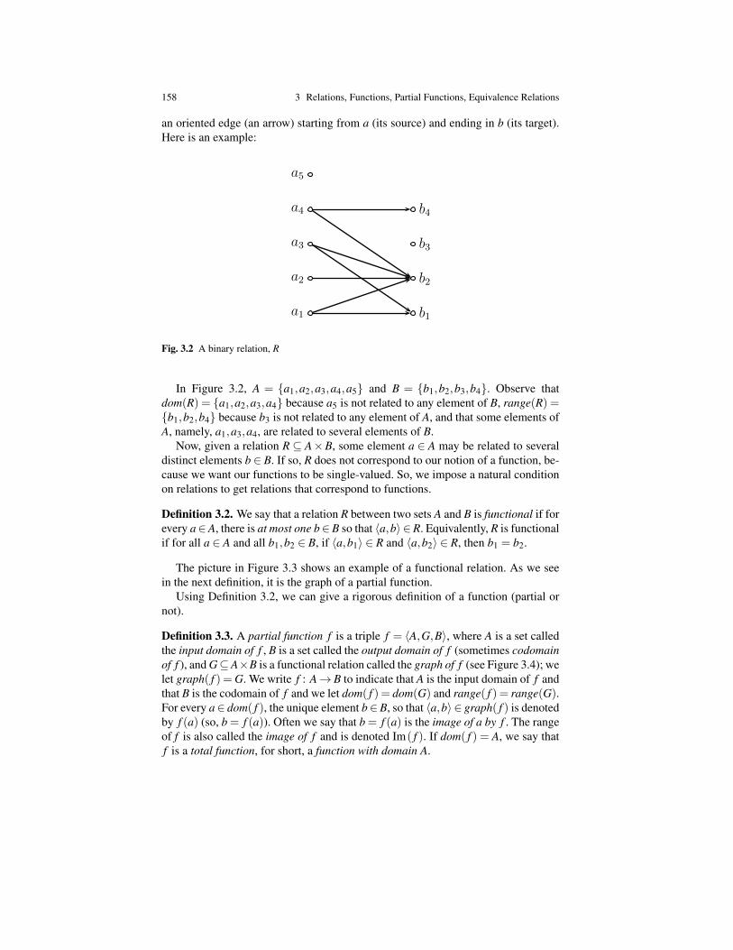
158 3 Relations, Functions, Partial Functions, Equivalence Relations
an oriented edge (an arrow) starting from a (its source) and ending in b (its target).Here is an example:
1
a1
a2
a3
a4
a5
b1
b2
b3
b4
Fig. 3.2 A binary relation, R
In Figure 3.2, A = a1,a2,a3,a4,a5 and B = b1,b2,b3,b4. Observe thatdom(R) = a1,a2,a3,a4 because a5 is not related to any element of B, range(R) =b1,b2,b4 because b3 is not related to any element of A, and that some elements ofA, namely, a1,a3,a4, are related to several elements of B.
Now, given a relation R ⊆ A×B, some element a ∈ A may be related to severaldistinct elements b ∈ B. If so, R does not correspond to our notion of a function, be-cause we want our functions to be single-valued. So, we impose a natural conditionon relations to get relations that correspond to functions.
Definition 3.2. We say that a relation R between two sets A and B is functional if forevery a∈A, there is at most one b∈B so that 〈a,b〉 ∈R. Equivalently, R is functionalif for all a ∈ A and all b1,b2 ∈ B, if 〈a,b1〉 ∈ R and 〈a,b2〉 ∈ R, then b1 = b2.
The picture in Figure 3.3 shows an example of a functional relation. As we seein the next definition, it is the graph of a partial function.
Using Definition 3.2, we can give a rigorous definition of a function (partial ornot).
Definition 3.3. A partial function f is a triple f = 〈A,G,B〉, where A is a set calledthe input domain of f , B is a set called the output domain of f (sometimes codomainof f ), and G⊆A×B is a functional relation called the graph of f (see Figure 3.4); welet graph( f ) = G. We write f : A→ B to indicate that A is the input domain of f andthat B is the codomain of f and we let dom( f ) = dom(G) and range( f ) = range(G).For every a∈ dom( f ), the unique element b∈B, so that 〈a,b〉 ∈ graph( f ) is denotedby f (a) (so, b = f (a)). Often we say that b = f (a) is the image of a by f . The rangeof f is also called the image of f and is denoted Im( f ). If dom( f ) = A, we say thatf is a total function, for short, a function with domain A.
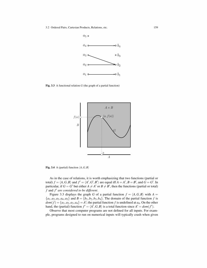
3.2 Ordered Pairs, Cartesian Products, Relations, etc. 159
1
a1
a2
a3
a4
a5
b1
b2
b3
b4
Fig. 3.3 A functional relation G (the graph of a partial function)
1
a
f(a) !a, f(a)"
G
A
B
A # B
Fig. 3.4 A (partial) function 〈A,G,B〉
As in the case of relations, it is worth emphasizing that two functions (partial ortotal) f = 〈A,G,B〉 and f ′ = 〈A′,G′,B′〉 are equal iff A = A′, B = B′, and G = G′. Inparticular, if G = G′ but either A 6= A′ or B 6= B′, then the functions (partial or total)f and f ′ are considered to be different.
Figure 3.3 displays the graph G of a partial function f = 〈A,G,B〉 with A =a1,a2,a3,a4,a5 and B = b1,b2,b3,b4. The domain of the partial function f isdom( f ) = a1,a2,a3,a4=A′; the partial function f is undefined at a4. On the otherhand, the (partial) function f ′ = 〈A′,G,B〉 is a total function since A′ = dom( f ′).
Observe that most computer programs are not defined for all inputs. For exam-ple, programs designed to run on numerical inputs will typically crash when given

160 3 Relations, Functions, Partial Functions, Equivalence Relations
strings as input. Thus, most computer programs compute partial functions that arenot total and it may be very hard to figure out what is the domain of these functions.This is a strong motivation for considering the notion of a partial function and notjust the notion of a (total) function.
Remarks:
1. If f = 〈A,G,B〉 is a partial function and b = f (a) for some a ∈ dom( f ), we saythat f maps a to b; we may write f : a 7→ b. For any b ∈ B, the set
a ∈ A | f (a) = b
is denoted f−1(b) and called the inverse image or preimage of b by f . (It is alsocalled the fibre of f above b. We explain this peculiar language later on.) Notethat f−1(b) 6= /0 iff b is in the image (range) of f . Often, a function, partial ornot, is called a map.
2. Note that Definition 3.3 allows A = /0. In this case, we must have G = /0 and,technically, 〈 /0, /0,B〉 is a total function. It is the empty function from /0 to B.
3. When a partial function is a total function, we don’t call it a “partial total func-tion,” but simply a “function.” The usual practice is that the term “function”refers to a total function. However, sometimes we say “total function” to stressthat a function is indeed defined on all of its input domain.
4. Note that if a partial function f = 〈A,G,B〉 is not a total function, then dom( f ) 6=A and for all a ∈ A−dom( f ), there is no b ∈ B so that 〈a,b〉 ∈ graph( f ). Thiscorresponds to the intuitive fact that f does not produce any output for any valuenot in its domain of definition. We can imagine that f “blows up” for this input(as in the situation where the denominator of a fraction is 0) or that the programcomputing f loops indefinitely for that input.
5. If f = 〈A,G,B〉 is a total function and A 6= /0, then B 6= /0.6. For any set A, the identity relation idA, is actually a function idA : A→ A.7. Given any two sets A and B, the rules 〈a,b〉 7→ a = pr1(〈a,b〉) and 〈a,b〉 7→ b =
pr2(〈a,b〉) make pr1 and pr2 into functions pr1 : A×B→A and pr2 : A×B→Bcalled the first and second projections.
8. A function f : A→ B is sometimes denoted Af−→ B. Some authors use a dif-
ferent kind of arrow to indicate that f is partial, for example, a dotted or dashedarrow. We do not go that far.
9. The set of all functions, f : A→ B, is denoted by BA. If A and B are finite, A hasm elements and B has n elements, it is easy to prove that BA has nm elements.
The reader might wonder why, in the definition of a (total) function, f : A→ B,we do not require B = Im f , inasmuch as we require that dom( f ) = A.
The reason has to do with experience and convenience. It turns out that in mostcases, we know what the domain of a function is, but it may be very hard to deter-mine exactly what its image is. Thus, it is more convenient to be flexible about thecodomain. As long as we know that f maps into B, we are satisfied.
For example, consider functions f : R→R2 from the real line into the plane. Theimage of such a function is a curve in the plane R2. Actually, to really get “decent”
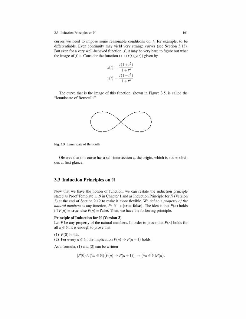
3.3 Induction Principles on N 161
curves we need to impose some reasonable conditions on f , for example, to bedifferentiable. Even continuity may yield very strange curves (see Section 3.13).But even for a very well-behaved function, f , it may be very hard to figure out whatthe image of f is. Consider the function t 7→ (x(t),y(t)) given by
x(t) =t(1+ t2)
1+ t4
y(t) =t(1− t2)
1+ t4 .
The curve that is the image of this function, shown in Figure 3.5, is called the“lemniscate of Bernoulli.”
Fig. 3.5 Lemniscate of Bernoulli
Observe that this curve has a self-intersection at the origin, which is not so obvi-ous at first glance.
3.3 Induction Principles on N
Now that we have the notion of function, we can restate the induction principlestated as Proof Template 1.19 in Chapter 1 and as Induction Principle for N (Version2) at the end of Section 2.12 to make it more flexible. We define a property of thenatural numbers as any function, P : N→true, false. The idea is that P(n) holdsiff P(n) = true, else P(n) = false. Then, we have the following principle.
Principle of Induction for N (Version 3).Let P be any property of the natural numbers. In order to prove that P(n) holds forall n ∈ N, it is enough to prove that
(1) P(0) holds.(2) For every n ∈ N, the implication P(n)⇒ P(n+1) holds.
As a formula, (1) and (2) can be written
[P(0)∧ (∀n ∈ N)(P(n)⇒ P(n+1))]⇒ (∀n ∈ N)P(n).
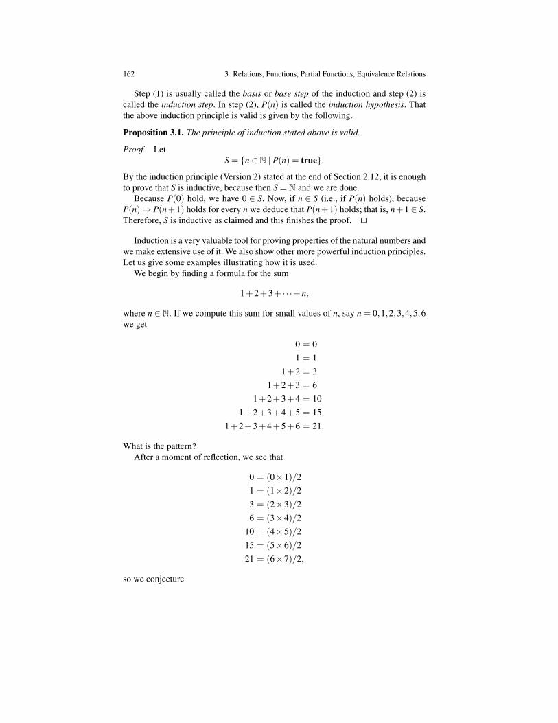
162 3 Relations, Functions, Partial Functions, Equivalence Relations
Step (1) is usually called the basis or base step of the induction and step (2) iscalled the induction step. In step (2), P(n) is called the induction hypothesis. Thatthe above induction principle is valid is given by the following.
Proposition 3.1. The principle of induction stated above is valid.
Proof . LetS = n ∈ N | P(n) = true.
By the induction principle (Version 2) stated at the end of Section 2.12, it is enoughto prove that S is inductive, because then S = N and we are done.
Because P(0) hold, we have 0 ∈ S. Now, if n ∈ S (i.e., if P(n) holds), becauseP(n)⇒ P(n+1) holds for every n we deduce that P(n+1) holds; that is, n+1 ∈ S.Therefore, S is inductive as claimed and this finishes the proof. ut
Induction is a very valuable tool for proving properties of the natural numbers andwe make extensive use of it. We also show other more powerful induction principles.Let us give some examples illustrating how it is used.
We begin by finding a formula for the sum
1+2+3+ · · ·+n,
where n ∈ N. If we compute this sum for small values of n, say n = 0,1,2,3,4,5,6we get
0 = 01 = 1
1+2 = 31+2+3 = 6
1+2+3+4 = 101+2+3+4+5 = 15
1+2+3+4+5+6 = 21.
What is the pattern?After a moment of reflection, we see that
0 = (0×1)/21 = (1×2)/23 = (2×3)/26 = (3×4)/2
10 = (4×5)/215 = (5×6)/221 = (6×7)/2,
so we conjecture
3.3 Induction Principles on N 163
Claim 1:
1+2+3+ · · ·+n =n(n+1)
2,
where n ∈ N.For the basis of the induction, where n = 0, we get 0 = 0, so the base step holds.For the induction step, for any n ∈ N, assume that
1+2+3+ · · ·+n =n(n+1)
2.
Consider 1+2+3+ · · ·+n+(n+1). Then, using the induction hypothesis, we have
1+2+3+ · · ·+n+(n+1) =n(n+1)
2+n+1
=n(n+1)+2(n+1)
2
=(n+1)(n+2)
2,
establishing the induction hypothesis and therefore proving our formula. utNext, let us find a formula for the sum of the first n+1 odd numbers:
1+3+5+ · · ·+2n+1,
where n ∈ N. If we compute this sum for small values of n, say n = 0,1,2,3,4,5,6we get
1 = 11+3 = 4
1+3+5 = 91+3+5+7 = 16
1+3+5+7+9 = 251+3+5+7+9+11 = 36
1+3+5+7+9+11+13 = 49.
This time, it is clear what the pattern is: we get perfect squares. Thus, we conjectureClaim 2:
1+3+5+ · · ·+2n+1 = (n+1)2,
where n ∈ N.For the basis of the induction, where n = 0, we get 1 = 12, so the base step holds.For the induction step, for any n ∈ N, assume that
1+3+5+ · · ·+2n+1 = (n+1)2.
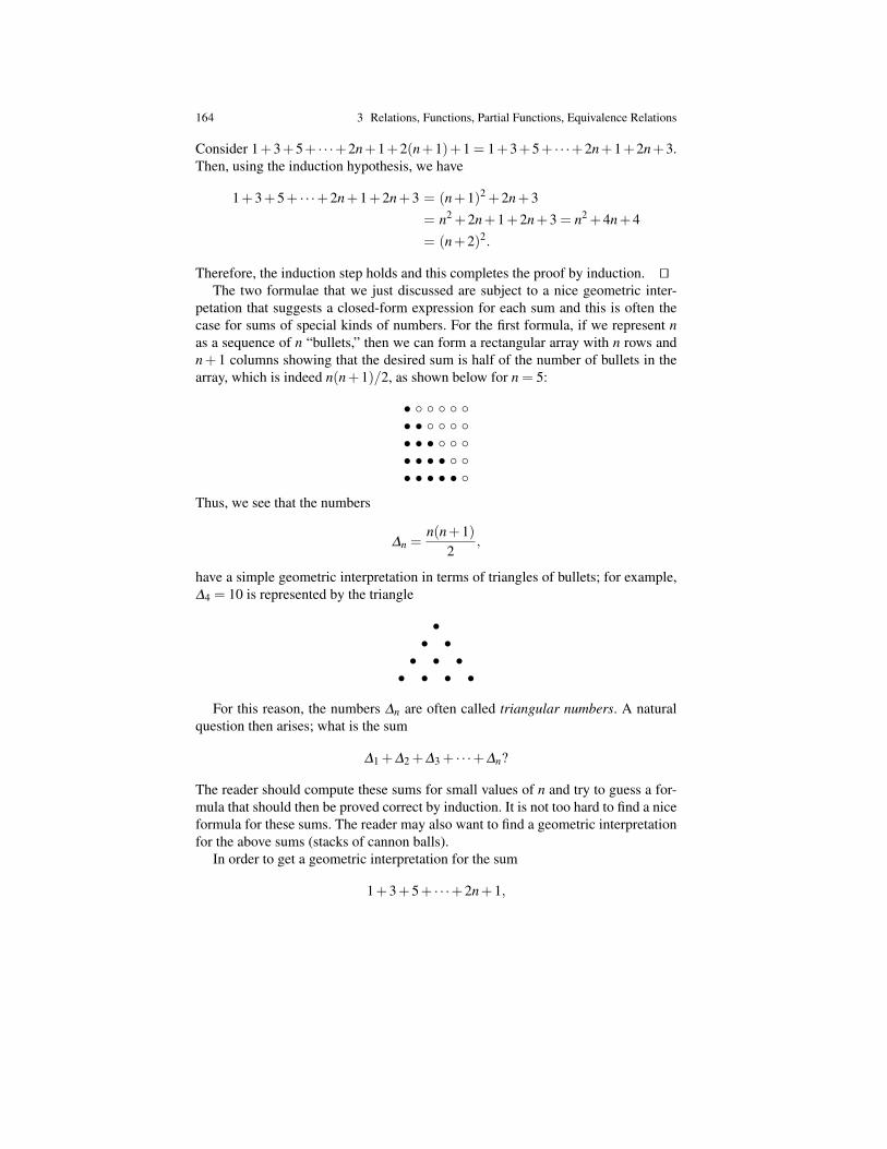
164 3 Relations, Functions, Partial Functions, Equivalence Relations
Consider 1+3+5+ · · ·+2n+1+2(n+1)+1 = 1+3+5+ · · ·+2n+1+2n+3.Then, using the induction hypothesis, we have
1+3+5+ · · ·+2n+1+2n+3 = (n+1)2 +2n+3= n2 +2n+1+2n+3 = n2 +4n+4= (n+2)2.
Therefore, the induction step holds and this completes the proof by induction. utThe two formulae that we just discussed are subject to a nice geometric inter-
petation that suggests a closed-form expression for each sum and this is often thecase for sums of special kinds of numbers. For the first formula, if we represent nas a sequence of n “bullets,” then we can form a rectangular array with n rows andn+ 1 columns showing that the desired sum is half of the number of bullets in thearray, which is indeed n(n+1)/2, as shown below for n = 5:
• • • • • • • • • • • • • • •
Thus, we see that the numbers
∆n =n(n+1)
2,
have a simple geometric interpretation in terms of triangles of bullets; for example,∆4 = 10 is represented by the triangle
•• •• • •• • • •
For this reason, the numbers ∆n are often called triangular numbers. A naturalquestion then arises; what is the sum
∆1 +∆2 +∆3 + · · ·+∆n?
The reader should compute these sums for small values of n and try to guess a for-mula that should then be proved correct by induction. It is not too hard to find a niceformula for these sums. The reader may also want to find a geometric interpretationfor the above sums (stacks of cannon balls).
In order to get a geometric interpretation for the sum
1+3+5+ · · ·+2n+1,
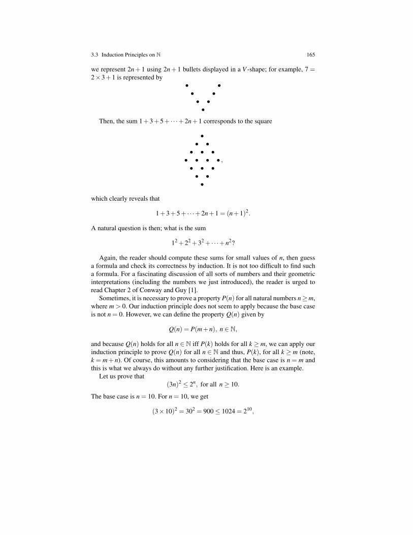
3.3 Induction Principles on N 165
we represent 2n+ 1 using 2n+ 1 bullets displayed in a V -shape; for example, 7 =2×3+1 is represented by
• •• •• ••
Then, the sum 1+3+5+ · · ·+2n+1 corresponds to the square
•• •• • •• • • •• • •• ••
,
which clearly reveals that
1+3+5+ · · ·+2n+1 = (n+1)2.
A natural question is then; what is the sum
12 +22 +32 + · · ·+n2?
Again, the reader should compute these sums for small values of n, then guessa formula and check its correctness by induction. It is not too difficult to find sucha formula. For a fascinating discussion of all sorts of numbers and their geometricinterpretations (including the numbers we just introduced), the reader is urged toread Chapter 2 of Conway and Guy [1].
Sometimes, it is necessary to prove a property P(n) for all natural numbers n≥m,where m > 0. Our induction principle does not seem to apply because the base caseis not n = 0. However, we can define the property Q(n) given by
Q(n) = P(m+n), n ∈ N,
and because Q(n) holds for all n ∈ N iff P(k) holds for all k ≥ m, we can apply ourinduction principle to prove Q(n) for all n ∈ N and thus, P(k), for all k ≥ m (note,k = m+ n). Of course, this amounts to considering that the base case is n = m andthis is what we always do without any further justification. Here is an example.
Let us prove that(3n)2 ≤ 2n, for all n≥ 10.
The base case is n = 10. For n = 10, we get
(3×10)2 = 302 = 900≤ 1024 = 210,

166 3 Relations, Functions, Partial Functions, Equivalence Relations
which is indeed true. Let us now prove the induction step. Assuming that (3n)2 ≤ 2n
holds for all n≥ 10, we want to prove that (3(n+1))2 ≤ 2n+1. As
(3(n+1))2 = (3n+3)2 = (3n)2 +18n+9,
if we can prove that 18n+9 ≤ (3n)2 when n ≥ 10, using the induction hypothesis,(3n)2 ≤ 2n, we have
(3(n+1))2 = (3n)2 +18n+9≤ (3n)2 +(3n)2 ≤ 2n +2n = 2n+1,
establishing the induction step. However,
(3n)2− (18n+9) = (3n−3)2−18
and (3n−3)2 ≥ 18 as soon as n≥ 3, so 18n+9≤ (3n)2 when n≥ 10, as required.Observe that the formula (3n)2≤ 2n fails for n= 9, because (3×9)2 = 272 = 729
and 29 = 512, but 729 > 512. Thus, the base has to be n = 10.There is another induction principle which is often more flexible than our original
induction principle. This principle, called complete induction (or sometimes stronginduction), is stated below.
Complete Induction Principle for N.In order to prove that a property (also called a predicate) P(n) holds for all n ∈N
it is enough to prove that
(1) P(0) holds (the base case).(2) For every m ∈ N, if (∀k ∈ N)(k ≤ m⇒ P(k)) then P(m+1).
The difference between ordinary induction and complete induction is that in com-plete induction, the induction hypothesis (∀k∈N)(k≤m⇒P(k)) assumes that P(k)holds for all k ≤ m and not just for m (as in ordinary induction), in order to deduceP(m+ 1). This gives us more proving power as we have more knowledge in orderto prove P(m+1). Complete induction is discussed more extensively in Section 7.3and its validity is proved as a consequence of the fact that every nonempty subset ofN has a smallest element but we can also justify its validity as follows. Define Q(m)by
Q(m) = (∀k ∈ N)(k ≤ m⇒ P(k)).
Then, it is an easy exercise to show that if we apply our (ordinary) induction princi-ple to Q(m) (induction principle, Version 3), then we get the principle of completeinduction. Here is an example of a proof using complete induction.
Define the sequence of natural numbers Fn (Fibonacci sequence) by
F1 = 1, F2 = 1, Fn+2 = Fn+1 +Fn, n≥ 1.
We claim that
Fn ≥3n−3
2n−4 , n≥ 4.

3.3 Induction Principles on N 167
Fig. 3.6 Leonardo P. Fibonacci, 1170–1250
The base case corresponds to n = 4, where
F4 = 3≥ 31
20 = 3,
which is true. Note that we also need to consider the case n = 5 by itself before wedo the induction step because even though F5 = F4 +F3, the induction hypothesisonly applies to F4 (n≥ 4 in the inequality above). We have
F5 = 5≥ 32
21 =92,
which is true because 10 > 9. Now for the induction step where n≥ 4, we have
Fn+2 = Fn+1 +Fn
≥ 3n−2
2n−3 +3n−3
2n−4
≥ 3n−3
2n−4
(1+
32
)=
3n−3
2n−352≥ 3n−3
2n−494=
3n−1
2n−2 ,
since 5/2 > 9/4, which concludes the proof of the induction step. Observe that weused the induction hypothesis for both Fn+1 and Fn in order to deduce that it holdsfor Fn+2. This is where we needed the extra power of complete induction.
Remark: The Fibonacci sequence Fn is really a function from N to N defined recur-sively but we haven’t proved yet that recursive definitions are legitimate methods fordefining functions. In fact, certain restrictions are needed on the kind of recursionused to define functions. This topic is explored further in Section 3.5. Using resultsfrom Section 3.5, it can be shown that the Fibonacci sequence is a well-definedfunction (but this does not follow immediately from Theorem 3.1).
Induction proofs can be subtle and it might be instructive to see some examplesof faulty induction proofs.
Assertion 1: For every natural numbers n ≥ 1, the number n2−n+11 is an oddprime (recall that a prime number is a natural number p≥ 2, which is only divisibleby 1 and itself).

168 3 Relations, Functions, Partial Functions, Equivalence Relations
Proof . We use induction on n≥ 1. For the base case n = 1, we have 12−1+11 =11, which is an odd prime, so the induction step holds.
Assume inductively that n2−n+11 is prime. Then, as
(n+1)2− (n+1)+11 = n2 +2n+1−n−1+11 = n2 +n+11,
we see that(n+1)2− (n+1)+11 = n2−n+11+2n.
By the induction hypothesis, n2−n+11 is an odd prime p, and because 2n is even,p+2n is odd and therefore prime, establishing the induction hypothesis. ut
If we compute n2− n+ 11 for n = 1,2, . . . ,10, we find that these numbers areindeed all prime, but for n = 11, we get
121 = 112−11+11 = 11×11,
which is not prime.Where is the mistake?What is wrong is the induction step: the fact that n2− n+ 11 is prime does not
imply that (n+1)2− (n+1)+11 = n2 +n+11 is prime, as illustrated by n = 10.Our “proof” of the induction step is nonsense.
The lesson is: the fact that a statement holds for many values of n ∈ N does notimply that it holds for all n ∈ N (or all n≥ k, for some fixed k ∈ N).
Interestingly, the prime numbers k, so that n2−n+k is prime for n = 1,2, . . . ,k−1, are all known (there are only six of them). It can be shown that these are the primenumbers k such that 1− 4k is a Heegner number, where the Heegner numbers arethe nine integers:
−1, −2, −3, −7, −11, −19, −43, −67, −163.
The above results are hard to prove and require some deep theorems of numbertheory. What can also be shown (and you should prove it) is that no nonconstantpolynomial takes prime numbers as values for all natural numbers.
Assertion 2: Every Fibonacci number Fn is even.Proof . For the base case, F3 = 2, which is even, so the base case holds.
Assume inductively that Fm is even for all m≤ n, with n≥ 3. Then, as
Fn+1 = Fn +Fn−1
and as both Fn and Fn−1 are even by the induction hypothesis (we are using completeinduction), we conclude that Fn+1 is even. ut
However, Assertion 2 is clearly false, because the Fibonacci sequence beginswith
1, 1, 2, 3, 5, 8, 13, 21, 34, . . . .
This time, the mistake is that we did not check the two base cases, F1 = 1 and F2 = 1.
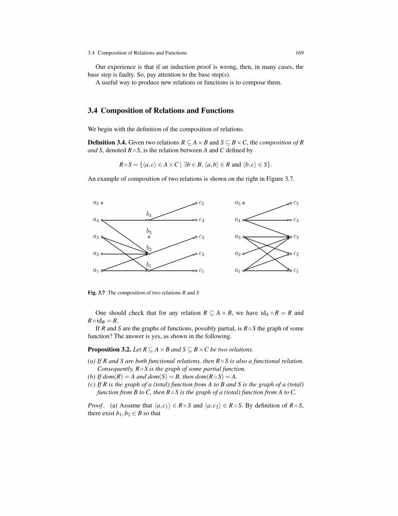
3.4 Composition of Relations and Functions 169
Our experience is that if an induction proof is wrong, then, in many cases, thebase step is faulty. So, pay attention to the base step(s).
A useful way to produce new relations or functions is to compose them.
3.4 Composition of Relations and Functions
We begin with the definition of the composition of relations.
Definition 3.4. Given two relations R⊆ A×B and S ⊆ B×C, the composition of Rand S, denoted RS, is the relation between A and C defined by
RS = 〈a,c〉 ∈ A×C | ∃b ∈ B, 〈a,b〉 ∈ R and 〈b,c〉 ∈ S.
An example of composition of two relations is shown on the right in Figure 3.7.
a1
a2
a3
a4
a5
b1
b2
b3
b4
c1
c2
c3
c4
c5
a1
a2
a3
a4
a5
c1
c2
c3
c4
c5
Fig. 3.7 The composition of two relations R and S
One should check that for any relation R ⊆ A× B, we have idA R = R andR idB = R.
If R and S are the graphs of functions, possibly partial, is RS the graph of somefunction? The answer is yes, as shown in the following.
Proposition 3.2. Let R⊆ A×B and S⊆ B×C be two relations.
(a) If R and S are both functional relations, then RS is also a functional relation.Consequently, RS is the graph of some partial function.
(b) If dom(R) = A and dom(S) = B, then dom(RS) = A.(c) If R is the graph of a (total) function from A to B and S is the graph of a (total)
function from B to C, then RS is the graph of a (total) function from A to C.
Proof . (a) Assume that 〈a,c1〉 ∈ R S and 〈a,c2〉 ∈ R S. By definition of R S,there exist b1,b2 ∈ B so that
170 3 Relations, Functions, Partial Functions, Equivalence Relations
〈a,b1〉 ∈ R, 〈b1,c1〉 ∈ S,
〈a,b2〉 ∈ R, 〈b2,c2〉 ∈ S.
As R is functional, 〈a,b1〉 ∈ R and 〈a,b2〉 ∈ R implies b1 = b2. Let b = b1 = b2, sothat 〈b1,c1〉 = 〈b,c1〉 and 〈b2,c2〉 = 〈b,c2〉. But, S is also functional, so 〈b,c1〉 ∈ Sand 〈b,c2〉 ∈ S implies that c1 = c2, which proves that RS is functional.
(b) If A = /0 then R = /0 and so RS = /0, which implies that dom(RS) = /0 = A.If A 6= /0, pick any a ∈ A. The fact that dom(R) = A 6= /0 means that there is someb ∈ B so that 〈a,b〉 ∈ R and so, B 6= /0. As dom(S) = B 6= /0, there is some c ∈ Cso that 〈b,c〉 ∈ S. Then, by the definition of R S, we see that 〈a,c〉 ∈ R S. Theargument holds for any a ∈ A, therefore we deduce that dom(RS) = A.
(c) If R and S are the graphs of partial functions, then this means that they arefunctional and (a) implies that R S is also functional. This shows that R S is thegraph of the partial function 〈A,RS,C〉. If R and S are the graphs of total functions,then dom(R) = A and dom(S) = B. By (b), we deduce that dom(RS) = A. By thefirst part of (c), RS is the graph of the partial function 〈A,RS,C〉, which is a totalfunction, inasmuch as dom(RS) = A. ut
Proposition 3.2 shows that it is legitimate to define the composition of functions,possibly partial. Thus, we make the following definition.
Definition 3.5. Given two functions f : A→ B and g : B→C, possibly partial, thecomposition of f and g, denoted g f , is the function (possibly partial)
g f = 〈A,graph( f )graph(g),C〉.
The reader must have noticed that the composition of two functions f : A→B andg : B→C is denoted g f , whereas the graph of g f is denoted graph( f )graph(g).This “reversal” of the order in which function composition and relation compositionare written is unfortunate and somewhat confusing.
Once again, we are the victims of tradition. The main reason for writing functioncomposition as g f is that traditionally the result of applying a function f to anargument x is written f (x). Then, (g f )(x) = g( f (x)), because z = (g f )(x) iffthere is some y so that y = f (x) and z = g(y); that is, z = g( f (x)). Some people,in particular algebraists, write function composition as f g, but then, they writethe result of applying a function f to an argument x as x f . With this convention,x( f g) = (x f )g, which also makes sense.
We prefer to stick to the convention where we write f (x) for the result of applyinga function f to an argument x and, consequently, we use the notation g f for thecomposition of f with g, even though it is the opposite of the convention for writingthe composition of relations.
Given any three relations, R⊆A×B, S⊆B×C, and T ⊆C×D, the reader shouldverify that
(RS)T = R (ST ).
We say that composition is associative. Similarly, for any three functions (possiblypartial), f : A→ B, g : B→ C, and h : C→ D, we have (associativity of function

3.5 Recursion on N 171
composition)(hg) f = h (g f ).
3.5 Recursion on N
The following situation often occurs. We have some set A, some fixed element a∈A,some function g : A→ A, and we wish to define a new function h : N→ A, so that
h(0) = a,
h(n+1) = g(h(n)) for all n ∈ N.
This way of defining h is called a recursive definition (or a definition by primitiverecursion). I would be surprised if any computer scientist had any trouble with this“definition” of h but how can we justify rigorously that such a function exists and isunique?
Indeed, the existence (and uniqueness) of h requires proof. The proof, althoughnot really hard, is surprisingly involved and in fact quite subtle. For those reasons,we do not give a proof of the following theorem but instead the main idea of theproof. The reader will find a complete proof in Enderton [2] (Chapter 4).
Theorem 3.1. (Recursion theorem on N) Given any set A, any fixed element a ∈ A,and any function g : A→ A, there is a unique function h : N→ A, so that
h(0) = a,
h(n+1) = g(h(n)) for all n ∈ N.
Proof . The idea is to approximate h. To do this, define a function f to be acceptableiff
1. dom( f )⊆ N and range( f )⊆ A.2. If 0 ∈ dom( f ), then f (0) = a.3. If n+1 ∈ dom( f ), then n ∈ dom( f ) and f (n+1) = g( f (n)).
Let F be the collection of all acceptable functions and set
h =⋃
F .
All we can say, so far, is that h is a relation. We claim that h is the desired function.For this, four things need to be proved:
1. The relation h is a function.2. The function h is acceptable.3. The function h has domain N.4. The function h is unique.
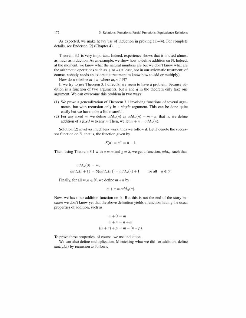
172 3 Relations, Functions, Partial Functions, Equivalence Relations
As expected, we make heavy use of induction in proving (1)–(4). For completedetails, see Enderton [2] (Chapter 4). ut
Theorem 3.1 is very important. Indeed, experience shows that it is used almostas much as induction. As an example, we show how to define addition on N. Indeed,at the moment, we know what the natural numbers are but we don’t know what arethe arithmetic operations such as + or ∗ (at least, not in our axiomatic treatment; ofcourse, nobody needs an axiomatic treatment to know how to add or multiply).
How do we define m+n, where m,n ∈ N?If we try to use Theorem 3.1 directly, we seem to have a problem, because ad-
dition is a function of two arguments, but h and g in the theorem only take oneargument. We can overcome this problem in two ways:
(1) We prove a generalization of Theorem 3.1 involving functions of several argu-ments, but with recursion only in a single argument. This can be done quiteeasily but we have to be a little careful.
(2) For any fixed m, we define addm(n) as addm(n) = m+ n; that is, we defineaddition of a fixed m to any n. Then, we let m+n = addm(n).
Solution (2) involves much less work, thus we follow it. Let S denote the succes-sor function on N, that is, the function given by
S(n) = n+ = n+1.
Then, using Theorem 3.1 with a = m and g = S, we get a function, addm, such that
addm(0) = m,
addm(n+1) = S(addm(n)) = addm(n)+1 for all n ∈ N.
Finally, for all m,n ∈ N, we define m+n by
m+n = addm(n).
Now, we have our addition function on N. But this is not the end of the story be-cause we don’t know yet that the above definition yields a function having the usualproperties of addition, such as
m+0 = m
m+n = n+m
(m+n)+ p = m+(n+ p).
To prove these properties, of course, we use induction.We can also define multiplication. Mimicking what we did for addition, define
multm(n) by recursion as follows.
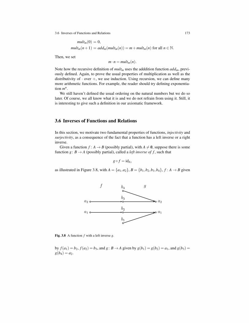
3.6 Inverses of Functions and Relations 173
multm(0) = 0,multm(n+1) = addm(multm(n)) = m+multm(n) for all n ∈ N.
Then, we setm ·n = multm(n).
Note how the recursive definition of multm uses the adddition function addm, previ-ously defined. Again, to prove the usual properties of multiplication as well as thedistributivity of · over +, we use induction. Using recursion, we can define manymore arithmetic functions. For example, the reader should try defining exponentia-tion mn.
We still haven’t defined the usual ordering on the natural numbers but we do solater. Of course, we all know what it is and we do not refrain from using it. Still, itis interesting to give such a definition in our axiomatic framework.
3.6 Inverses of Functions and Relations
In this section, we motivate two fundamental properties of functions, injectivity andsurjectivity, as a consequence of the fact that a function has a left inverse or a rightinverse.
Given a function f : A→ B (possibly partial), with A 6= /0, suppose there is somefunction g : B→ A (possibly partial), called a left inverse of f , such that
g f = idA,
as illustrated in Figure 3.8, with A = a1,a2, B = b1,b2,b3,b4, f : A→ B given
a1
a2
b1
b2
b3
b4
a1
a2
f g
Fig. 3.8 A function f with a left inverse g.
by f (a1) = b2, f (a2) = b3, and g : B→ A given by g(b1) = g(b2) = a1, and g(b3) =g(b4) = a2.
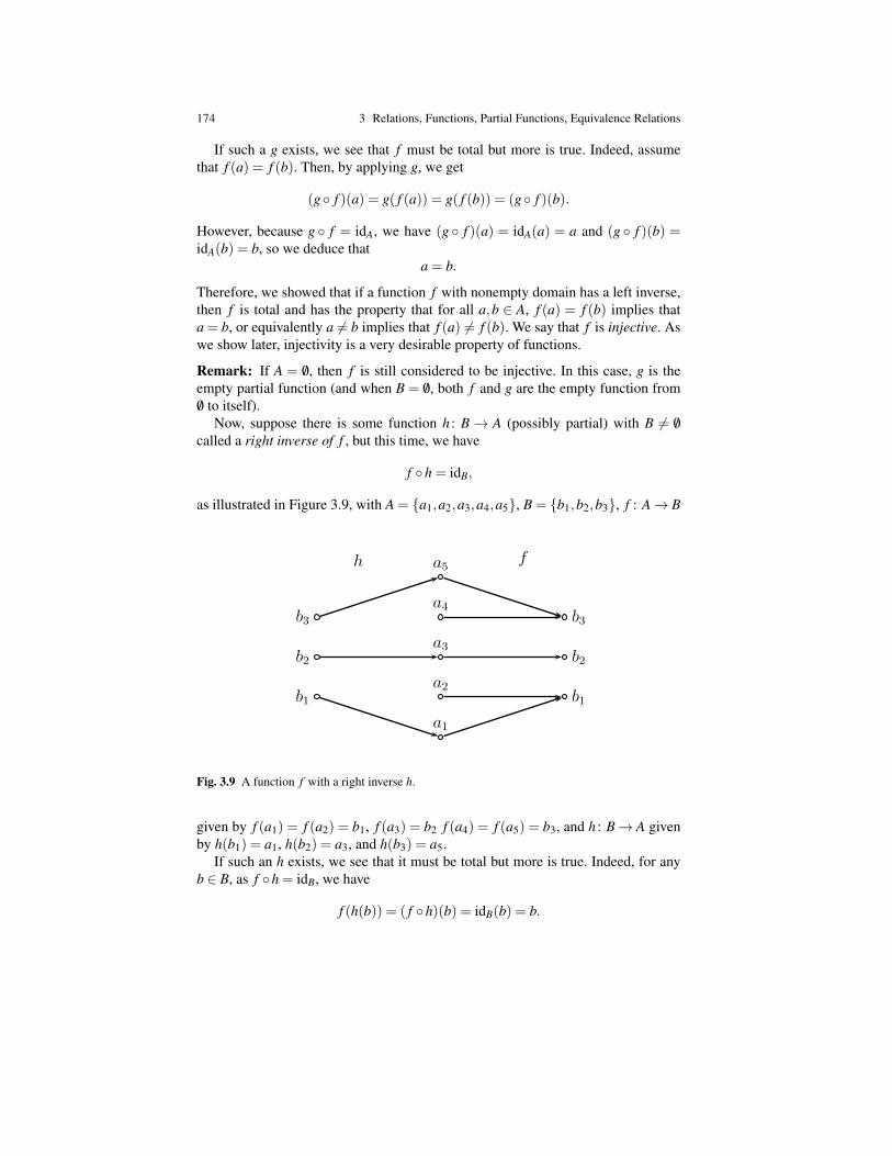
174 3 Relations, Functions, Partial Functions, Equivalence Relations
If such a g exists, we see that f must be total but more is true. Indeed, assumethat f (a) = f (b). Then, by applying g, we get
(g f )(a) = g( f (a)) = g( f (b)) = (g f )(b).
However, because g f = idA, we have (g f )(a) = idA(a) = a and (g f )(b) =idA(b) = b, so we deduce that
a = b.
Therefore, we showed that if a function f with nonempty domain has a left inverse,then f is total and has the property that for all a,b ∈ A, f (a) = f (b) implies thata = b, or equivalently a 6= b implies that f (a) 6= f (b). We say that f is injective. Aswe show later, injectivity is a very desirable property of functions.
Remark: If A = /0, then f is still considered to be injective. In this case, g is theempty partial function (and when B = /0, both f and g are the empty function from/0 to itself).
Now, suppose there is some function h : B→ A (possibly partial) with B 6= /0called a right inverse of f , but this time, we have
f h = idB,
as illustrated in Figure 3.9, with A = a1,a2,a3,a4,a5, B = b1,b2,b3, f : A→ B
b1
b2
b3
a1
a2
a3
a4
a5
b1
b2
b3
h f
Fig. 3.9 A function f with a right inverse h.
given by f (a1) = f (a2) = b1, f (a3) = b2 f (a4) = f (a5) = b3, and h : B→ A givenby h(b1) = a1, h(b2) = a3, and h(b3) = a5.
If such an h exists, we see that it must be total but more is true. Indeed, for anyb ∈ B, as f h = idB, we have
f (h(b)) = ( f h)(b) = idB(b) = b.

3.6 Inverses of Functions and Relations 175
Therefore, we showed that if a function f with nonempty codomain has a rightinverse h then h is total and f has the property that for all b∈ B, there is some a∈ A,namely, a = h(b), so that f (a) = b. In other words, Im( f ) = B or equivalently, everyelement in B is the image by f of some element of A. We say that f is surjective.Again, surjectivity is a very desirable property of functions.
Remark: If B = /0, then f is still considered to be surjective but h is not total unlessA = /0, in which case f is the empty function from /0 to itself.
If a function has a left inverse (respectively, a right inverse), then it may havemore than one left inverse (respectively, right inverse).
If a function (possibly partial) f : A→ B with A,B 6= /0 happens to have both aleft inverse g : B→ A and a right inverse h : B→ A, then we know that f and h aretotal. We claim that g = h, so that g is total and moreover g is uniquely determinedby f .
Lemma 3.1. Let f : A→ B be any function and suppose that f has a left inverseg : B→ A and a right inverse h : B→ A. Then, g = h and, moreover, g is unique,which means that if g′ : B→ A is any function that is both a left and a right inverseof f , then g′ = g.
Proof . Assume thatg f = idA and f h = idB.
Then, we have
g = g idB = g ( f h) = (g f )h = idA h = h.
Therefore, g = h. Now, if g′ is any other left inverse of f and h′ is any other rightinverse of f , the above reasoning applied to g and h′ shows that g = h′ and the samereasoning applied to g′ and h′ shows that g′ = h′. Therefore, g′ = h′ = g = h, that is,g is uniquely determined by f . ut
This leads to the following definition.
Definition 3.6. A function f : A→ B is said to be invertible iff there is a functiong : B→ A which is both a left inverse and a right inverse; that is,
g f = idA and f g = idB.
In this case, we know that g is unique and it is denoted f−1.
From the above discussion, if a function is invertible, then it is both injective andsurjective. This shows that a function generally does not have an inverse. In orderto have an inverse a function needs to be injective and surjective, but this fails to betrue for many functions. It turns out that if a function is injective and surjective thenit has an inverse. We prove this in the next section.
The notion of inverse can also be defined for relations, but it is a somewhatweaker notion.
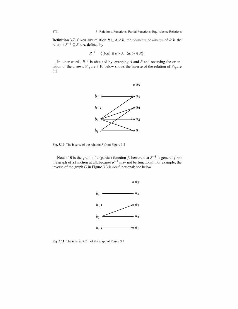
176 3 Relations, Functions, Partial Functions, Equivalence Relations
Definition 3.7. Given any relation R ⊆ A×B, the converse or inverse of R is therelation R−1 ⊆ B×A, defined by
R−1 = 〈b,a〉 ∈ B×A | 〈a,b〉 ∈ R.
In other words, R−1 is obtained by swapping A and B and reversing the orien-tation of the arrows. Figure 3.10 below shows the inverse of the relation of Figure3.2:
1
a1
a2
a3
a4
a5
b1
b2
b3
b4
Fig. 3.10 The inverse of the relation R from Figure 3.2
Now, if R is the graph of a (partial) function f , beware that R−1 is generally notthe graph of a function at all, because R−1 may not be functional. For example, theinverse of the graph G in Figure 3.3 is not functional; see below.
1
a1
a2
a3
a4
a5
b1
b2
b3
b4
Fig. 3.11 The inverse, G−1, of the graph of Figure 3.3

3.7 Injections, Surjections, Bijections, Permutations 177
The above example shows that one has to be careful not to view a function asa relation in order to take its inverse. In general, this process does not produce afunction. This only works if the function is invertible.
Given any two relations, R⊆ A×B and S⊆ B×C, the reader should prove that
(RS)−1 = S−1 R−1.
(Note the switch in the order of composition on the right-hand side.) Similarly, iff : A→ B and g : B→C are any two invertible functions, then g f is invertible and
(g f )−1 = f−1 g−1.
3.7 Injections, Surjections, Bijections, Permutations
We encountered injectivity and surjectivity in Section 3.6. For the record, let us givethe following.
Definition 3.8. Given any function f : A→ B, we say that f is injective (or one-to-one) iff for all a,b ∈ A, if f (a) = f (b), then a = b, or equivalently, if a 6= b, thenf (a) 6= f (b). We say that f is surjective (or onto) iff for every b ∈ B, there is somea ∈ A so that b = f (a), or equivalently if Im( f ) = B. The function f is bijectiveiff it is both injective and surjective. When A = B, a bijection f : A→ A is called apermutation of A.
Remarks:
1. If A = /0, then any function, f : /0→ B is (trivially) injective.2. If B = /0, then f is the empty function from /0 to itself and it is (trivially) surjec-
tive.3. A function, f : A→ B, is not injective iff there exist a,b ∈ A with a 6= b and
yet f (a) = f (b); see Figure 3.12.4. A function, f : A→ B, is not surjective iff for some b ∈ B, there is no a ∈ A
with b = f (a); see Figure 3.13.5. We have Im f = b ∈ B | (∃a ∈ A)(b = f (a)), thus a function f : A→ B is
always surjective onto its image.6. The notation f : A → B is often used to indicate that a function f : A→ B is an
injection.7. If A 6= /0, a function f : A→ B is injective iff for every b ∈ B, there at most one
a ∈ A such that b = f (a).8. If A 6= /0, a function f : A→ B is surjective iff for every b ∈ B, there at least one
a ∈ A such that b = f (a) iff f−1(b) 6= /0 for all b ∈ B.9. If A 6= /0, a function f : A→ B is bijective iff for every b ∈ B, there is a unique
a ∈ A such that b = f (a).10. When A is the finite set A = 1, . . . ,n, also denoted [n], it is not hard to show
that there are n! permutations of [n].

178 3 Relations, Functions, Partial Functions, Equivalence Relations
1
a
b
f(a) = f(b)A
B
Fig. 3.12 A noninjective function
1
b
fA
B
Im(f)
Fig. 3.13 A nonsurjective function
The function f1 : Z→ Z given by f1(x) = x+1 is injective and surjective. How-ever, the function f2 : Z→ Z given by f2(x) = x2 is neither injective nor surjective(why?). The function f3 : Z→ Z given by f3(x) = 2x is injective but not surjective.The function f4 : Z→ Z given by
f4(x) =k if x = 2k
k if x = 2k+1
is surjective but not injective.
Remark: The reader should prove that if A and B are finite sets, A has m elementsand B has n elements (m≤ n) then the set of injections from A to B has
n!(n−m)!
elements. The following theorem relates the notions of injectivity and surjectivity tothe existence of left and right inverses.
Theorem 3.2. Let f : A→ B be any function and assume A 6= /0.
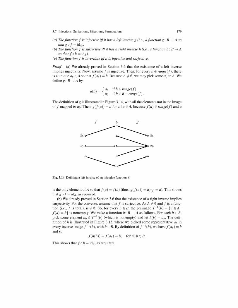
3.7 Injections, Surjections, Bijections, Permutations 179
(a) The function f is injective iff it has a left inverse g (i.e., a function g : B→ A sothat g f = idA).
(b) The function f is surjective iff it has a right inverse h (i.e., a function h : B→ Aso that f h = idB).
(c) The function f is invertible iff it is injective and surjective.
Proof . (a) We already proved in Section 3.6 that the existence of a left inverseimplies injectivity. Now, assume f is injective. Then, for every b ∈ range( f ), thereis a unique ab ∈ A so that f (ab) = b. Because A 6= /0, we may pick some a0 in A. Wedefine g : B→ A by
g(b) =
ab if b ∈ range( f )a0 if b ∈ B− range( f ).
The definition of g is illustrated in Figure 3.14, with all the elements not in the imageof f mapped to a0. Then, g( f (a)) = a for all a ∈ A, because f (a) ∈ range( f ) and a
ab
b
a0a0
ab
f g
Fig. 3.14 Defining a left inverse of an injective function f .
is the only element of A so that f (a) = f (a) (thus, g( f (a)) = a f (a) = a). This showsthat g f = idA, as required.
(b) We already proved in Section 3.6 that the existence of a right inverse impliessurjectivity. For the converse, assume that f is surjective. As A 6= /0 and f is a func-tion (i.e., f is total), B 6= /0. So, for every b ∈ B, the preimage f−1(b) = a ∈ A |f (a) = b is nonempty. We make a function h : B→ A as follows. For each b ∈ B,pick some element ab ∈ f−1(b) (which is nonempty) and let h(b) = ab. The defi-nition of h is illustrated in Figure 3.15, where we picked some representative ab inevery inverse image f−1(b), with b∈ B. By definition of f−1(b), we have f (ab) = band so,
f (h(b)) = f (ab) = b, for all b ∈ B.
This shows that f h = idB, as required.
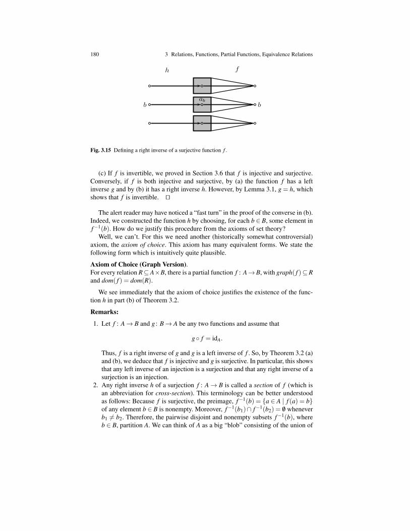
180 3 Relations, Functions, Partial Functions, Equivalence Relations
bab
b
h f
Fig. 3.15 Defining a right inverse of a surjective function f .
(c) If f is invertible, we proved in Section 3.6 that f is injective and surjective.Conversely, if f is both injective and surjective, by (a) the function f has a leftinverse g and by (b) it has a right inverse h. However, by Lemma 3.1, g = h, whichshows that f is invertible. ut
The alert reader may have noticed a “fast turn” in the proof of the converse in (b).Indeed, we constructed the function h by choosing, for each b ∈ B, some element inf−1(b). How do we justify this procedure from the axioms of set theory?
Well, we can’t. For this we need another (historically somewhat controversial)axiom, the axiom of choice. This axiom has many equivalent forms. We state thefollowing form which is intuitively quite plausible.
Axiom of Choice (Graph Version).For every relation R⊆A×B, there is a partial function f : A→B, with graph( f )⊆Rand dom( f ) = dom(R).
We see immediately that the axiom of choice justifies the existence of the func-tion h in part (b) of Theorem 3.2.
Remarks:
1. Let f : A→ B and g : B→ A be any two functions and assume that
g f = idA.
Thus, f is a right inverse of g and g is a left inverse of f . So, by Theorem 3.2 (a)and (b), we deduce that f is injective and g is surjective. In particular, this showsthat any left inverse of an injection is a surjection and that any right inverse of asurjection is an injection.
2. Any right inverse h of a surjection f : A→ B is called a section of f (which isan abbreviation for cross-section). This terminology can be better understoodas follows: Because f is surjective, the preimage, f−1(b) = a ∈ A | f (a) = bof any element b ∈ B is nonempty. Moreover, f−1(b1)∩ f−1(b2) = /0 wheneverb1 6= b2. Therefore, the pairwise disjoint and nonempty subsets f−1(b), whereb ∈ B, partition A. We can think of A as a big “blob” consisting of the union of

3.8 Direct Image and Inverse Image 181
the sets f−1(b) (called fibres) and lying over B. The function f maps each fibre,f−1(b) onto the element, b ∈ B. Then, any right inverse h : B→ A of f picksout some element in each fibre, f−1(b), forming a sort of horizontal section ofA shown as a curve in Figure 3.16.
1
f
f!1(b1)
h
B
A
b1 b2
h(b2)
Fig. 3.16 A section h of a surjective function f .
3. Any left inverse g of an injection f : A→ B is called a retraction of f . The ter-minology reflects the fact that intuitively, as f is injective (thus, g is surjective),B is bigger than A and because g f = idA, the function g “squeezes” B onto Ain such a way that each point b = f (a) in Im f is mapped back to its ancestora ∈ A. So, B is “retracted” onto A by g.
Before discussing direct and inverse images, we define the notion of restrictionand extension of functions.
Definition 3.9. Given two functions, f : A→C and g : B→C, with A ⊆ B, we saythat f is the restriction of g to A if graph( f )⊆ graph(g); we write f = g A. In thiscase, we also say that g is an extension of f to B.
If f : A→C is a restriction of g : B→C to A (with A⊆ B), then for every a ∈ Awe have f (a) = g(a), but g is defined on a larger set than f . For example, if A = N(the natural numbers) and B =C =Q (the rational numbers), and if f : N→Q andg : Q→Q are given by f (x) = x/2 and g(x) = x/2, then f is the restriction of g toN and g is an extension of f to Q.
3.8 Direct Image and Inverse Image
A function f : X→Y induces a function from 2X to 2Y also denoted f and a functionfrom 2Y to 2X , as shown in the following definition.
182 3 Relations, Functions, Partial Functions, Equivalence Relations
Definition 3.10. Given any function f : X → Y , we define the function f : 2X → 2Y
so that, for every subset A of X ,
f (A) = y ∈ Y | ∃x ∈ A, y = f (x).
The subset f (A) of Y is called the direct image of A under f , for short, the image ofA under f . We also define the function f−1 : 2Y → 2X so that, for every subset B ofY ,
f−1(B) = x ∈ X | ∃y ∈ B, y = f (x).The subset f−1(B) of X is called the inverse image of B under f or the preimage ofB under f .
Remarks:
1. The overloading of notation where f is used both for denoting the original func-tion f : X → Y and the new function f : 2X → 2Y may be slightly confusing. Ifwe observe that f (x) = f (x), for all x∈X , we see that the new f is a naturalextension of the old f to the subsets of X and so, using the same symbol f forboth functions is quite natural after all. To avoid any confusion, some authors(including Enderton) use a different notation for f (A), for example, f [[A]]. Weprefer not to introduce more notation and we hope that which f we are dealingwith is made clear by the context.
2. The use of the notation f−1 for the function f−1 : 2Y → 2X may even be moreconfusing, because we know that f−1 is generally not a function from Y to X .However, it is a function from 2Y to 2X . Again, some authors use a differentnotation for f−1(B), for example, f−1[[A]]. We stick to f−1(B).
3. The set f (A) is sometimes called the push-forward of A along f and f−1(B) issometimes called the pullback of B along f .
4. Observe that f−1(y) = f−1(y), where f−1(y) is the preimage defined justafter Definition 3.3.
5. Although this may seem counterintuitive, the function f−1 has a better behaviorthan f with respect to union, intersection, and complementation.
Some useful properties of f : 2X → 2Y and f−1 : 2Y → 2X are now stated withoutproof. The proofs are easy and left as exercises.
Proposition 3.3. Given any function f : X → Y , the following properties hold.
(1) For any B⊆ Y , we havef ( f−1(B))⊆ B.
(2) If f : X → Y is surjective, then
f ( f−1(B)) = B.
(3) For any A⊆ X, we haveA⊆ f−1( f (A)).
3.9 Equivalence Relations and Partitions 183
(4) If f : X → Y is injective, then
A = f−1( f (A)).
The next proposition deals with the behavior of f : 2X → 2Y and f−1 : 2Y → 2X
with respect to union, intersection, and complementation.
Proposition 3.4. Given any function f : X → Y the following properties hold.
(1) For all A,B⊆ X, we have
f (A∪B) = f (A)∪ f (B).
(2)f (A∩B)⊆ f (A)∩ f (B).
Equality holds if f : X → Y is injective.(3)
f (A)− f (B)⊆ f (A−B).
Equality holds if f : X → Y is injective.(4) For all C,D⊆ Y , we have
f−1(C∪D) = f−1(C)∪ f−1(D).
(5)f−1(C∩D) = f−1(C)∩ f−1(D).
(6)f−1(C−D) = f−1(C)− f−1(D).
As we can see from Proposition 3.4, the function f−1 : 2Y → 2X has better be-havior than f : 2X → 2Y with respect to union, intersection, and complementation.
3.9 Equivalence Relations and Partitions
Equivalence relations play a fundamental role in mathematics and computer science.Intuitively, the notion of an equivalence relation is a generalization of the notion ofequality. Since the equality relation satisfies the properties that
1. a = a, for all a;2. If a = b and b = c, then a = c, for all a,b,c;3. If a = b, then b = a, for all a,b;
we postulate axioms that capture these properties.
Definition 3.11. A binary relation R on a set X is an equivalence relation iff it isreflexive, transitive, and symmetric, that is:
184 3 Relations, Functions, Partial Functions, Equivalence Relations
(1) (Reflexivity): aRa, for all a ∈ X(2) (Transitivity): If aRb and bRc, then aRc, for all a,b,c ∈ X(3) (Symmetry): If aRb, then bRa, for all a,b ∈ X
Here are some examples of equivalence relations.
1. The identity relation idX on a set X is an equivalence relation.2. The relation X×X is an equivalence relation.3. Let S be the set of students in CIS160. Define two students to be equivalent iff
they were born the same year. It is trivial to check that this relation is indeed anequivalence relation.
4. Given any natural number p≥ 1, we can define a relation on Z as follows,
n≡ m (mod p)
iff p divides n−m; that is, n = m+ pk, for some k ∈ Z. It is an easy exercise tocheck that this is indeed an equivalence relation called congruence modulo p.
5. Equivalence of propositions is the relation defined so that P ≡ Q iff P⇒ Qand Q⇒ P are both provable (say, classically). It is easy to check that logicalequivalence is an equivalence relation.
6. Suppose f : X → Y is a function. Then, we define the relation ≡ f on X by
x≡ f y iff f (x) = f (y).
It is immediately verified that ≡ f is an equivalence relation. Actually, we showthat every equivalence relation arises in this way, in terms of (surjective) func-tions.
The crucial property of equivalence relations is that they partition their domainX into pairwise disjoint nonempty blocks. Intuitively, they carve out X into a bunchof puzzle pieces.
Definition 3.12. Given an equivalence relation R on a set X for any x ∈ X , the set
[x]R = y ∈ X | xRy
is the equivalence class of x. Each equivalence class [x]R is also denoted xR and thesubscript R is often omitted when no confusion arises. The set of equivalence classesof R is denoted by X/R. The set X/R is called the quotient of X by R or quotient ofX modulo R. The function, π : X → X/R, given by
π(x) = [x]R, x ∈ X ,
is called the canonical projection (or projection) of X onto X/R.
Every equivalence relation is reflexive, that is, xRx for every x ∈ X , thereforeobserve that x ∈ [x]R for any x ∈ R; that is, every equivalence class is nonempty. Itis also clear that the projection π : X → X/R is surjective. The main properties ofequivalence classes are given by the following.
3.9 Equivalence Relations and Partitions 185
Proposition 3.5. Let R be an equivalence relation on a set X. For any two elementsx,y ∈ X we have
xRy iff [x] = [y].
Moreover, the equivalence classes of R satisfy the following properties.
(1) [x] 6= /0, for all x ∈ X(2) If [x] 6= [y] then [x]∩ [y] = /0(3) X =
⋃x∈X [x].
Proof . First, assume that [x] = [y]. We observed that by reflexivity, y ∈ [y]. As[x] = [y], we get y ∈ [x] and by definition of [x], this means that xRy.
Next, assume that xRy. Let us prove that [y] ⊆ [x]. Pick any z ∈ [y]; this meansthat yRz. By transitivity, we get xRz; that is, z ∈ [x], proving that [y] ⊆ [x]. Now, asR is symmetric, xRy implies that yRx and the previous argument yields [x] ⊆ [y].Therefore, [x] = [y], as needed.
Property (1) follows from the fact that x ∈ [x] (by reflexivity).Let us prove the contrapositive of (2). So, assume [x]∩ [y] 6= /0. Thus, there is
some z so that z ∈ [x] and z ∈ [y]; that is,
xRz and yRz.
By symmetry, we get zRy and by transitivity, xRy. But then, by the first part of theproposition, we deduce [x] = [y], as claimed.
The third property follows again from the fact that x ∈ [x]. ut
A useful way of interpreting Proposition 3.5 is to say that the equivalence classesof an equivalence relation form a partition, as defined next.
Definition 3.13. Given a set X , a partition of X is any family Π = Xii∈I , of subsetsof X such that
(1) Xi 6= /0, for all i ∈ I (each Xi is nonempty)(2) If i 6= j then Xi∩X j = /0 (the Xi are pairwise disjoint)(3) X =
⋃i∈I Xi (the family is exhaustive).
Each set Xi is called a block of the partition.
In the example where equivalence is determined by the same year of birth, eachequivalence class consists of those students having the same year of birth. Let usnow go back to the example of congruence modulo p (with p > 0) and figure outwhat are the blocks of the corresponding partition. Recall that
m≡ n (mod p)
iff m− n = pk for some k ∈ Z. By the division theorem (Theorem 7.7), we knowthat there exist some unique q,r, with m = pq+ r and 0≤ r ≤ p−1. Therefore, forevery m ∈ Z,
m≡ r (mod p) with 0≤ r ≤ p−1,
186 3 Relations, Functions, Partial Functions, Equivalence Relations
which shows that there are p equivalence classes, [0], [1], . . . , [p− 1], where theequivalence class [r] (with 0≤ r ≤ p−1) consists of all integers of the form pq+ r,where q ∈ Z, that is, those integers whose residue modulo p is r.
Proposition 3.5 defines a map from the set of equivalence relations on X to theset of partitions on X . Given any set X , let Equiv(X) denote the set of equivalencerelations on X and let Part(X) denote the set of partitions on X . Then, Proposition3.5 defines the function Π : Equiv(X)→ Part(X) given by,
Π(R) = X/R = [x]R | x ∈ X,
where R is any equivalence relation on X . We also write ΠR instead of Π(R).There is also a function R : Part(X)→ Equiv(X) that assigns an equivalence
relation to a partition as shown by the next proposition.
Proposition 3.6. For any partition Π = Xii∈I on a set X, the relation R(Π) de-fined by
xR(Π)y iff (∃i ∈ I)(x,y ∈ Xi),
is an equivalence relation whose equivalence classes are exactly the blocks Xi.
Proof . By property (iii) of a partition (in Definition 3.13), every x ∈ X belongs tosome subset Xi for some index i ∈ I. Furthermore, the index i such that x ∈ Xi isunique, since otherwise we would have x ∈ Xi ∩X j for some i 6= j, contradicting(ii). The fact that R(Π) is reflexive is trivial, since x ∈ Xi for some (unique) i ∈ I.If xR(Π)y and yR(Π)z, then x,y ∈ Xi for some unique index i ∈ I and y,z ∈ X jfor some unique index j ∈ I. Since y ∈ Xi and y ∈ X j, by uniqueness of the indexof the subset containing y, we must have i = j, and then x,z ∈ Xi, which showsthat xR(Π)z; that is, R(Π) is transitive. Since xR(Π)y means that x,y ∈ Xi forsome (unique) index i ∈ I, we also have y,x ∈ Xi; that is, yR(Π)x, which shows thatR(Π) is symmetric. Therefore, R(Π) is an equivalence relation. For all x,y ∈ X ,since xR(Π)y iff x,y ∈ Xi for some i ∈ I, it is clear that the equivalence class of xis equal to Xi. Also, since each Xi is nonempty, every Xi is an equivalence class ofR(Π), so the equivalence classes of R(Π) are exactly the Xi. ut
Putting Propositions 3.5 and 3.6 together we obtain the useful fact that there isa bijection between Equiv(X) and Part(X). Therefore, in principle, it is a matter oftaste whether we prefer to work with equivalence relations or partitions. In computerscience, it is often preferable to work with partitions, but not always.
Proposition 3.7. Given any set X the functions Π : Equiv(X)→ Part(X) andR : Part(X)→ Equiv(X) are mutual inverses; that is,
R Π = id and Π R = id.
Consequently, there is a bijection between the set Equiv(X) of equivalence relationson X and the set Part(X) of partitions on X.
3.9 Equivalence Relations and Partitions 187
Proof . This is a routine verification left to the reader. ut
Now, if f : X → Y is a surjective function, we have the equivalence relation ≡ fdefined by
x≡ f y iff f (x) = f (y).
It is clear that the equivalence class of any x ∈ X is the inverse image f−1( f (x)),of f (x) ∈ Y . Therefore, there is a bijection between X/ ≡ f and Y . Thus, we canidentify f and the projection π , from X onto X/≡ f . If f is not surjective, note thatf is surjective onto f (X) and so, we see that f can be written as the composition
f = iπ,
where π : X → f (X) is the canonical projection and i : f (X)→ Y is the inclusionfunction mapping f (X) into Y (i.e., i(y) = y, for every y ∈ f (X)).
Given a set X , the inclusion ordering on X ×X defines an ordering on binaryrelations on X ,2 namely,
R≤ S iff (∀x,y ∈ X)(xRy⇒ xSy).
When R≤ S, we say that R refines S.If R and S are equivalence relations and R ≤ S, we observe that every equiva-
lence class of R is contained in some equivalence class of S. Actually, in view ofProposition 3.5, we see that every equivalence class of S is the (disjoint) union ofequivalence classes of R.
As an example, if S is the equivalence relation where two students in a class areequivalent if they were both the same year, and R is the equivalence relation wheretwo students are equivalent if they were both the same year and the same month,then R is a refinement of S. Each equivalence class of R contains students born thesame year (say 1995) and the same month (say July), and each equivalence class ofS contains students born the same year and is the (disjoint) union of the equivalenceclasses (of R) consisting of students born the same month of that year (say January,March, December of 1995).
Note that idX is the least equivalence relation on X and X×X is the largest equiv-alence relation on X . This suggests the following questions: Given two equivalencerelations R and S,
1. Is there a greatest equivalence relation contained in both R and S, called themeet of R and S?
2. Is there a smallest equivalence relation containing both R and S, called the joinof R and S?
The answer is yes in both cases. It is easy to see that the meet of two equivalencerelations is R∩ S, their intersection. But beware, their join is not R∪ S, becausein general, R∪ S is not transitive. However, there is a least equivalence relation
2 For a precise definition of the notion of ordering, see Section 7.1.

188 3 Relations, Functions, Partial Functions, Equivalence Relations
containing R and S, and this is the join of R and S. This leads us to look at variousclosure properties of relations.
3.10 Transitive Closure, Reflexive and Transitive Closure,Smallest Equivalence Relation
Let R be any relation on a set X . Note that R is reflexive iff idX ⊆ R. Consequently,the smallest reflexive relation containing R is idX ∪R. This relation is called thereflexive closure of R.
We claim that R is transitive iff RR⊆ R.Proof . If R is transitive, then for any pair (x,z) ∈ R R, there is some y ∈ X suchthat (x,y) ∈ R and (y,z) ∈ R, and by transitivity of R, we have (x,z) ∈ R, whichshows that RR⊆ R. Conversely, assume that RR⊆ R. If (x,y) ∈ R and (y,z) ∈ R,then (x,z) ∈ RR, and since RR⊆ R, we have (x,z) ∈ R; thus R is transitive. ut
This suggests a way of making the smallest transitive relation containing R (if Ris not already transitive). Define Rn by induction as follows.
R0 = idX
Rn+1 = Rn R.
It is easy to prove by induction that
Rn+1 = Rn R = RRn for all n≥ 0.
Definition 3.14. Given any relation R on a set X , the transitive closure of R is therelation R+ given by
R+ =⋃n≥1
Rn.
The reflexive and transitive closure of R is the relation R∗, given by
R∗ =⋃n≥0
Rn = idX ∪R+.
Proposition 3.8. Given any relation R on a set X, the relation R+ is the smallesttransitive relation containing R and R∗ is the smallest reflexive and transitive rela-tion containing R.
Proof . By definition of R+, we have R ⊆ R+. First, let us prove that R+ is tran-sitive. Since R+ =
⋃k≥1 Rk, if (x,y) ∈ R+, then (x,y) ∈ Rm for some m ≥ 1, and
if (y,z) ∈ R+, then (x,y) ∈ Rn for some n ≥ 1. Consequently, (x,z) ∈ Rm+n, butRm+n ⊆⋃k≥1 Rk = R+, so (x,z) ∈ R+, which shows that R+ is transitive.
Secondly, we show that if S is any transitive relation containing R, then Rn ⊆ Sfor all n ≥ 1. We proceed by induction on n ≥ 1. The base case n = 1 simply says
3.10 Transitive Closure, Reflexive and Transitive Closure 189
that R ⊆ S, which holds by hypothesis. Now, it is easy to see that for any relationsR1,R2,S1,S2, if R1 ⊆ S1 and if R2 ⊆ S2, then R1 R2 ⊆ S1 S2. Going back to theinduction step, by the induction hypothesis Rn ⊆ S and by hypothesis R⊆ S. By thefact that we just stated and because S is transitive iff SS⊆ S, we get
Rn+1 = Rn R⊆ SS⊆ S,
establishing the induction step. Therefore, if R⊆ S and if S is transitive, then, Rn ⊆ Sfor all n≥ 1, so
R+ =⋃n≥1
Rn ⊆ S.
This proves that R+ is indeed the smallest transitive relation containing R.Next, consider R∗ = idX ∪R+. Since idX idX = idX , idX R+ = R+ idX = R+
and R+ is transitive, the relation R∗ is transitive. By definition of R∗, we have R⊆R∗,and since R0 = idX ⊆ R∗, the relation R∗ is reflexive.
Conversely, we prove that if S is any relations such that R ⊆ S and S is reflexiveand transtive, then Rn ⊆ S for all n≥ 0. The case n = 0 corresponds to the reflexivityof S (since R0 = idX ⊆ S), and for n ≥ 1, the proof is identical to the previous one.In summary, R∗ is the smallest reflexive and transitive relation containing R. ut
If R is reflexive, then idX ⊆ R, which implies that R ⊆ R2, so Rk ⊆ Rk+1 for allk ≥ 0. From this, we can show that if X is a finite set, then there is a smallest k sothat Rk = Rk+1. In this case, Rk is the reflexive and transitive closure of R. If X hasn elements it can be shown that k ≤ n−1.
Note that a relation R is symmetric iff R−1 = R. As a consequence, R∪R−1 isthe smallest symmetric relation containing R. This relation is called the symmetricclosure of R. Finally, given a relation R, what is the smallest equivalence relationcontaining R? The answer is given by
Proposition 3.9. For any relation R on a set X, the relation
(R∪R−1)∗
is the smallest equivalence relation containing R.
Proof . By Proposition 3.8, the relation (R∪R−1)∗ is reflexive and transitive andclearly it contains R, so we need to prove that (R∪R−1)∗ is symmetric. For this, itis sufficient to prove that every power (R∪R−1)n is symmetric for all n≥ 0. This iseasily done by induction. The base case n = 0 is trivial since (R∪R−1)0 = idX . Forthe induction step, since by the induction hypothesis,
((R∪R−1)n
)−1= (R∪R−1)n,
we have

190 3 Relations, Functions, Partial Functions, Equivalence Relations((R∪R−1)n+1)−1
=((R∪R−1)n (R∪R−1)
)−1
= (R∪R−1)−1 ((R∪R−1)n)−1
= (R∪R−1) (R∪R−1)n
= (R∪R−1)n+1;
that is, (R∪R−1)n+1 is symmetric. Therefore, (R∪R−1)∗ is an equivalence relationcontaining R.
Every equivalence relation S containing R must contain R∪R−1, and since S isa reflexive and transitive relation containing R∪R−1, by Proposition 3.8, S contains(R∪R−1)∗. ut
3.11 Equinumerosity; Cantor’s Theorem; The PigeonholePrinciple
The notion of size of a set is fairly intuitive for finite sets but what does it mean forinfinite sets? How do we give a precise meaning to the questions:
(a) Do X and Y have the same size?(b) Does X have more elements than Y ?
For finite sets, we can rely on the natural numbers. We count the elements in thetwo sets and compare the resulting numbers. If one of the two sets is finite and theother is infinite, it seems fair to say that the infinite set has more elements than thefinite one.
But what if both sets are infinite?
Remark: A critical reader should object that we have not yet defined what a finiteset is (or what an infinite set is). Indeed, we have not. This can be done in termsof the natural numbers but, for the time being, we rely on intuition. We should alsopoint out that when it comes to infinite sets, experience shows that our intuition failsus miserably. So, we should be very careful.
Let us return to the case where we have two infinite sets. For example, considerN and the set of even natural numbers, 2N= 0,2,4,6, . . .. Clearly, the second setis properly contained in the first. Does that make N bigger? On the other hand, thefunction n 7→ 2n is a bijection between the two sets, which seems to indicate thatthey have the same number of elements. Similarly, the set of squares of natural num-bers, Squares = 0,1,4,9,16,25, . . . is properly contained in N and many naturalnumbers are missing from Squares. But, the map n 7→ n2 is a bijection between Nand Squares, which seems to indicate that they have the same number of elements.
A more extreme example is provided by N×N and N. Intuitively, N×N is two-dimensional and N is one-dimensional, so N seems much smaller than N×N. How-ever, it is possible to construct bijections between N×N and N (try to find one). Infact, such a function J has the graph partially shown below:

3.11 Equinumerosity; Cantor’s Theorem; The Pigeonhole Principle 191
...3 6 . . .
2 3 7 . . .
1 1 4 8 . . .
0 0 2 5 90 1 2 3 . . .
The function J corresponds to a certain way of enumerating pairs of integers.Note that the value of m+n is constant along each diagonal, and consequently, wehave
J(m,n) = 1+2+ · · ·+(m+n)+m,
= ((m+n)(m+n+1)+2m)/2,= ((m+n)2 +3m+n)/2.
For example, J(2,1) = ((2+ 1)2 + 3 · 2+ 1)/2 = (9+ 6+ 1)/2 = 16/2 = 8. Thefunction
J(m,n) =12((m+n)2 +3m+n)
is a bijection but that’s not so easy to prove.Perhaps even more surprising, there are bijections between N and Q. What about
between R×R and R? Again, the answer is yes, but that’s harder to prove.These examples suggest that the notion of bijection can be used to define rigor-
ously when two sets have the same size. This leads to the concept of equinumerosity.
Definition 3.15. A set A is equinumerous to a set B, written A ≈ B, iff there is abijection f : A→ B. We say that A is dominated by B, written A B, iff there isan injection from A to B. Finally, we say that A is strictly dominated by B, writtenA≺ B, iff A B and A 6≈ B.
Using the above concepts, we can give a precise definition of finiteness. First,recall that for any n ∈ N, we defined [n] as the set [n] = 1,2, . . . ,n, with [0] = /0.
Definition 3.16. A set A is finite if it is equinumerous to a set of the form [n], forsome n ∈ N. A set A is infinite iff it is not finite. We say that A is countable (ordenumerable) iff A is dominated by N; that is, if there is an injection from A to N.
Two pretty results due to Cantor (1873) are given in the next theorem. These areamong the earliest results of set theory. We assume that the reader is familiar withthe fact that every number, x ∈ R, can be expressed in decimal expansion (possiblyinfinite). For example,
π = 3.14159265358979 · · ·
192 3 Relations, Functions, Partial Functions, Equivalence Relations
Theorem 3.3. (Cantor’s Theorem) (a) The set N is not equinumerous to the set Rof real numbers.
(b) For every set A there is no surjection from A onto 2A. Consequently, no set Ais equinumerous to its power set 2A.
Proof . (a) We use a famous proof method due to Cantor and known as a diagonalargument. We prove that if we assume there is a bijection f : N→ R, then there isa real number z not belonging to the image of f , contradicting the surjectivity of f .Now, if f exists, we can form a bi-infinite array
f (0) = k0.d01d02d03d04 · · · ,f (1) = k1.d11d12d13d14 · · · ,f (2) = k2.d21d22d23d24 · · · ,
...f (n) = kn.dn1dn2 · · ·dnn+1 · · · ,
...
where kn is the integer part of f (n) and the dni are the decimals of f (n), with i≥ 1.The number
z = 0.d1d2d3 · · ·dn+1 · · ·is defined so that dn+1 = 1 if dnn+1 6= 1, else dn+1 = 2 if dnn+1 = 1, for every n≥ 0,The definition of z shows that
dn+1 6= dnn+1, for all n≥ 0,
which implies that z is not in the above array; that is, z /∈ Im f .(b) The proof is a variant of Russell’s paradox. Assume that there is a surjection,
g : A→ 2A; we construct a set B ⊆ A that is not in the image of g, a contradiction.Consider the set
B = a ∈ A | a /∈ g(a).Obviously, B⊆ A. However, for every a ∈ A,
a ∈ B iff a /∈ g(a),
which shows that B 6= g(a) for all a ∈ A (because, if there was some a ∈ A suchthat g(a) = B, then from the above we would have a ∈ B iff a /∈ g(a) iff a /∈ B, acontradiction); that is, B is not in the image of g. ut
As there is an obvious injection of N into R, Theorem 3.3 shows that N is strictlydominated by R. Also, as we have the injection a 7→ a from A into 2A, we see thatevery set is strictly dominated by its power set. So, we can form sets as big as wewant by repeatedly using the power set operation.
Remark: In fact, R is equinumerous to 2N; see Problem 3.43.
3.11 Equinumerosity; Cantor’s Theorem; The Pigeonhole Principle 193
The following proposition shows an interesting connection between the notionof power set and certain sets of functions. To state this proposition, we need theconcept of characteristic function of a subset.
Given any set X for any subset A of X , define the characteristic function of A,denoted χA, as the function χA : X →0,1 given by
χA(x) =1 if x ∈ A
0 if x /∈ A.
In other words, χA tests membership in A. For any x ∈ X , χA(x) = 1 iff x ∈ A.Observe that we obtain a function χ : 2X → 0,1X from the power set of X to theset of characteristic functions from X to 0,1, given by
χ(A) = χA.
We also have the function, S : 0,1X → 2X , mapping any characteristic functionto the set that it defines and given by
S ( f ) = x ∈ X | f (x) = 1,
for every characteristic function, f ∈ 0,1X .
Proposition 3.10. For any set X the function χ : 2X → 0,1X from the power setof X to the set of characteristic functions on X is a bijection whose inverse isS : 0,1X → 2X .
Proof . Simply check that χ S = id and S χ = id, which is straightforward.ut
In view of Proposition 3.10, there is a bijection between the power set 2X and theset of functions in 0,1X . If we write 2 = 0,1, then we see that the two sets lookthe same. This is the reason why the notation 2X is often used for the power set (butothers prefer P(X)).
There are many other interesting results about equinumerosity. We only mentionfour more, all very important. Recall that [n] = 1,2, . . . ,n, for any n ∈ N.
Theorem 3.4. (Pigeonhole Principle) No set of the form [n] is equinumerous to aproper subset of itself, where n ∈ N,
Proof . Although the pigeonhole principle seems obvious, the proof is not. In fact,the proof requires induction. We advise the reader to skip this proof and come backto it later after we have given more examples of proof by induction.
Suppose we can prove the following claim.Claim. Whenever a function f : [n]→ [n] is an injection, then it is a surjection
onto [n] (and thus, a bijection).Observe that the above claim implies the pigeonhole principle. This is proved by
contradiction. So, assume there is a function f : [n]→ [n], such that f is injective andIm f =A⊆ [n] with A 6= [n]; that is, f is a bijection between [n] and A, a proper subset
194 3 Relations, Functions, Partial Functions, Equivalence Relations
of [n]. Because f : [n]→ [n] is injective, by the claim, we deduce that f : [n]→ [n]is surjective, that is, Im f = [n], contradicting the fact that Im f = A 6= [n].
It remains to prove by induction on n ∈N that if f : [n]→ [n] is an injection, thenit is a surjection (and thus, a bijection). For n = 0, f must be the empty function,which is a bijection.
Assume that the induction hypothesis holds for any n ≥ 0 and consider any in-jection, f : [n+1]→ [n+1]. Observe that the restriction of f to [n] is injective.
Case 1. The subset [n] is closed under f ; that is, f ([n]) ⊆ [n]. Then, we knowthat f [n] is injective and by the induction hypothesis, f ([n]) = [n]. Because f isinjective, we must have f (n+1) = n+1. Hence, f is surjective, as claimed.
Case 2. The subset [n] is not closed under f ; that is, there is some p≤ n such thatf (p) = n+ 1. Since p ≤ n and f is injective, f (n+ 1) 6= n+ 1, so f (n+ 1) ∈ [n].We can create a new injection f from [n+1] to itself with the same image as f byinterchanging two values of f so that [n] closed under f . Define f by
f (p) = f (n+1)
f (n+1) = f (p) = n+1
f (i) = f (i), 1≤ i≤ n, i 6= p.
Then, f is an injection from [n+1] to itself and [n] is closed under f . By Case 1, fis surjective, and as Im f = Im f , we conclude that f is also surjective. ut
Theorem 3.5. (Pigeonhole Principle for Finite Sets) No finite set is equinumerousto a proper subset of itself.
Proof . To say that a set A is finite is to say that there is a bijection g : A→ [n] forsome n∈N. Assume that there is a bijection f between A and some proper subset ofA. Then, consider the function g f g−1, from [n] to itself, as shown in the diagrambelow:
A
f
[n]g−1oo
g fg−1
A g
// [n]
Since by hypothesis f is a bijection onto some proper subset of A, there is someb ∈ A such that b /∈ f (A). Let p = g(b) ∈ [n]. We claim that p /∈ (g f g−1)([n]).
Otherwise, there would be some i ∈ [n] such that
(g f g−1)(i) = p = g(b),
and since g is invertible, we would have
f (g−1(i)) = b,
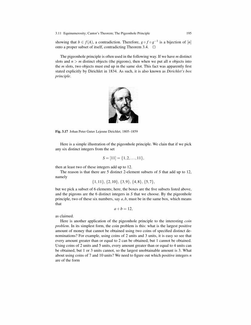
3.11 Equinumerosity; Cantor’s Theorem; The Pigeonhole Principle 195
showing that b ∈ f (A), a contradiction. Therefore, g f g−1 is a bijection of [n]onto a proper subset of itself, contradicting Theorem 3.4. ut
The pigeonhole principle is often used in the following way. If we have m distinctslots and n > m distinct objects (the pigeons), then when we put all n objects intothe m slots, two objects must end up in the same slot. This fact was apparently firststated explicitly by Dirichlet in 1834. As such, it is also known as Dirichlet’s boxprinciple.
Fig. 3.17 Johan Peter Gutav Lejeune Dirichlet, 1805–1859
Here is a simple illustration of the pigeonhole principle. We clain that if we pickany six distinct integers from the set
S = [11] = 1,2, . . . ,11,
then at least two of these integers add up to 12.The reason is that there are 5 distinct 2-element subsets of S that add up to 12,
namely1,11, 2,10, 3,9, 4,8, 5,7,
but we pick a subset of 6 elements; here, the boxes are the five subsets listed above,and the pigeons are the 6 distinct integers in S that we choose. By the pigeonholeprinciple, two of these six numbers, say a,b, must be in the same box, which meansthat
a+b = 12,
as claimed.Here is another application of the pigeonhole principle to the interesting coin
problem. In its simplest form, the coin problem is this: what is the largest positiveamount of money that cannot be obtained using two coins of specified distinct de-nominations? For example, using coins of 2 units and 3 units, it is easy so see thatevery amount greater than or equal to 2 can be obtained, but 1 cannot be obtained.Using coins of 2 units and 5 units, every amount greater than or equal to 4 units canbe obtained, but 1 or 3 units cannot, so the largest unobtainable amount is 3. Whatabout using coins of 7 and 10 units? We need to figure out which positive integers nare of the form

196 3 Relations, Functions, Partial Functions, Equivalence Relations
n = 7h+10k, with h,k ∈ N.
It turns out that every amount greater than or equal to 54 can be obtained, and 53 isthe largest amount that cannot be achieved. In general, we have the following result.
Theorem 3.6. Let p,q be any two positive integers such that 2≤ p < q, and assumethat p and q are relatively prime. Then, for any integer n ≥ (p− 1)(q− 1), thereexist some natural numbers h,k ∈ N such that
n = hp+ kq.
Furthermore, the largest integer not expressible in the above form is pq− p− q =(p−1)(q−1)−1.
Let us prove the first part of the theorem for all integers n such that n≥ pq.Proof . For this, consider the sequence
n, n−q, n−2q, . . . , n− (p−1)q.
We claim that some integer in this sequence is divisible by p.Observe that every number n− iq is nonnegative, so divide each n− iq by p,
obtaining the following sequence
r0,r1, . . . ,rp−1
of p remainders, with
n− ip = mi p+ ri, 0≤ ri ≤ p−1, mi ≥ 0,
for i = 0, . . . , p−1. The above is a sequence of p integers ri such that 0≤ ri ≤ p−1,so by the pigeonhole principle, if the ri are not all distinct, then two of them areidentical. Assume that ri = r j, with 0≤ i < j ≤ p−1. Then,
n− iq = mi p+ ri
n− jq = m j p+ r j
with ri = r j, so by subtraction we get
( j− i)q = (mi−m j)p.
Thus, p divides ( j− i)q, and since p and q are relatively prime, by Euclid’s lemma(see Proposition 7.9), p should divide j− i. But, 0 < j− i < p, a contradiction.Therefore, our remainders comprise all distinct p integers between 0 and p− 1,so one of them must be equal to 0, which proves that some number n− iq in thesequence is divisible by p. This shows that
n− iq = mi p,
so
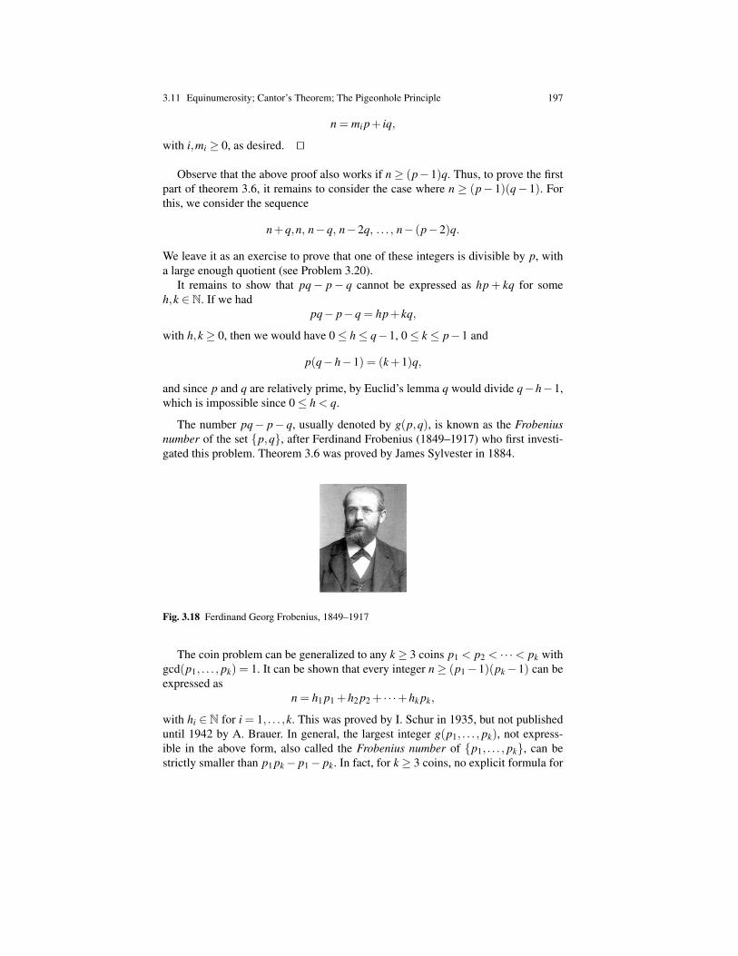
3.11 Equinumerosity; Cantor’s Theorem; The Pigeonhole Principle 197
n = mi p+ iq,
with i,mi ≥ 0, as desired. ut
Observe that the above proof also works if n≥ (p−1)q. Thus, to prove the firstpart of theorem 3.6, it remains to consider the case where n ≥ (p− 1)(q− 1). Forthis, we consider the sequence
n+q,n, n−q, n−2q, . . . , n− (p−2)q.
We leave it as an exercise to prove that one of these integers is divisible by p, witha large enough quotient (see Problem 3.20).
It remains to show that pq− p− q cannot be expressed as hp + kq for someh,k ∈ N. If we had
pq− p−q = hp+ kq,
with h,k ≥ 0, then we would have 0≤ h≤ q−1, 0≤ k ≤ p−1 and
p(q−h−1) = (k+1)q,
and since p and q are relatively prime, by Euclid’s lemma q would divide q−h−1,which is impossible since 0≤ h < q.
The number pq− p− q, usually denoted by g(p,q), is known as the Frobeniusnumber of the set p,q, after Ferdinand Frobenius (1849–1917) who first investi-gated this problem. Theorem 3.6 was proved by James Sylvester in 1884.
Fig. 3.18 Ferdinand Georg Frobenius, 1849–1917
The coin problem can be generalized to any k≥ 3 coins p1 < p2 < · · ·< pk withgcd(p1, . . . , pk) = 1. It can be shown that every integer n≥ (p1−1)(pk−1) can beexpressed as
n = h1 p1 +h2 p2 + · · ·+hk pk,
with hi ∈ N for i = 1, . . . ,k. This was proved by I. Schur in 1935, but not publisheduntil 1942 by A. Brauer. In general, the largest integer g(p1, . . . , pk), not express-ible in the above form, also called the Frobenius number of p1, . . . , pk, can bestrictly smaller than p1 pk− p1− pk. In fact, for k ≥ 3 coins, no explicit formula for
198 3 Relations, Functions, Partial Functions, Equivalence Relations
g(p1, . . . , pk) is known! For k = 3, there is a quadratic-time algoritm, but in general,it can be shown that computing the Frobenius number is hard (NP-hard).
As amusing version of the problem is the McNuggets number problem. McDon-ald’s sells boxes of chicken McNuggets in boxes of 6,9 and 20 nuggets. What is thelargest number of chicken McNuggets that can’t be purchased? It turns out to be 43nuggets!
Let us give another application of the pigeonhole principle involving sequencesof integers. Given a finite sequence S of integers a1, . . . ,an, a subsequence of S isa sequence b1, . . . ,bm, obtained by deleting elements from the original sequenceand keeping the remaining elements in the same order as they originally appeared.More precisely, b1, . . . ,bm is a subsequence of a1, . . . ,an if there is an injectiong : 1, . . . ,m→1, . . . ,n such that bi = ag(i) for all i∈ 1, . . . ,m and i≤ j impliesg(i)≤ g( j) for all i, j ∈ 1, . . . ,m. For example, the sequence
1 9 10 8 3 7 5 2 6 4
contains the subsequence9 8 6 4.
An increasing subsequence is a subsequence whose elements are in strictly increas-ing order and a decreasing subsequence is a subsequence whose elements are instrictly decreasing order. For example, 9 8 6 4 is a decreasing subsequence of ouroriginal sequence. We now prove the following beautiful result due to Erdos andSzekeres.
Theorem 3.7. (Erdos and Szekeres) Let n be any nonzero natural number. Every se-quence of n2+1 pairwise distinct natural numbers must contain either an increasingsubsequence or a decreasing subsequence of length n+1.
Proof . The proof proceeds by contradiction. So, assume there is a sequence S ofn2 +1 pairwise distinct natural numbers so that all increasing or decreasing subse-quences of S have length at most n. We assign to every element s of the sequence Sa pair of natural numbers (us,ds), called a label, where us, is the length of a longestincreasing subsequence of S that starts at s and where ds is the length of a longestdecreasing subsequence of S that starts at s.
There are no increasing or descreasing subsequences of length n+ 1 in S, thusobserve that 1≤ us,ds ≤ n for all s ∈ S. Therefore,
Claim 1: There are at most n2 distinct labels (us,ds), where s ∈ S.We also assert the following.Claim 2: If s and t are any two distinct elements of S, then (us,ds) 6= (ut ,dt).We may assume that s precedes t in S because otherwise we interchange s and t
in the following argument. Inasmuch as s 6= t, there are two cases:
(a) s < t. In this case, we know that there is an increasing subsequence of length utstarting with t. If we insert s in front of this subsequence, we get an increasingsubsequence of ut +1 elements starting at s. Then, as us is the maximal lengthof all increasing subsequences starting with s, we must have ut +1≤ us; that is,
3.12 Finite and Infinite Sets; The Schroder–Bernstein 199
us > ut ,
which implies (us,ds) 6= (ut ,dt).(b) s > t. This case is similar to case (a), except that we consider a decreasing
subsequence of length dt starting with t. We conclude that
ds > dt ,
which implies (us,ds) 6= (ut ,dt).
Therefore, in all cases, we proved that s and t have distinct labels.Now, by Claim 1, there are only n2 distinct labels and S has n2+1 elements so, by
the pigeonhole principle, two elements of S must have the same label. But, this con-tradicts Claim 2, which says that distinct elements of S have distinct labels. There-fore, S must have either an increasing subsequence or a decreasing subsequence oflength n+1, as originally claimed. ut
Remark: Note that this proof is not constructive in the sense that it does not pro-duce the desired subsequence; it merely asserts that such a sequence exists.
The following generalization of the Pigeonhole Principle is sometimes useful.The proof is left as an easy exercise.
Proposition 3.11. (Generalized Pigeonhole Principle) Let X and Y be two finite setsand k a positive integer. If |X |> k|Y |, then for every function f : X → Y , there exista least k+1 distinct element of X that are mapped by f to the same element of Y .
Here is an application of the Generalized Pigeonhole Principle. How large shoulda group of people be to guarantee that three members of the group have the sameinitials (first, middle, last)?
Since we implicitly assumed that our alphabet is the standard one with 26 lettersA, B, ..., Z, there are 263 possible triples of initials. In this problem, k = 2 (sothat k + 1 = 3), and if the number of people is p, by the Generalized PigeonholePrinciple, if p > 2×263, then three people will have the same initials, so we if pick2×263+1= 35,153 people, we are certain that three of them have the same initials.
3.12 Finite and Infinite Sets; The Schroder–Bernstein Theorem
Let A be a finite set. Then, by definition, there is a bijection f : A→ [n] for some n∈N. We claim that such an n is unique. Otherwise, there would be another bijectiong : A→ [p] for some p ∈ N with n 6= p. But now, we would have a bijection g f−1
between [n] and [p] with n 6= p. This would imply that there is either an injectionfrom [n] to a proper subset of itself or an injection from [p] to a proper subset ofitself,3 contradicting the pigeonhole principle.
3 Recall that n+ 1 = 0,1, . . . ,n = [n]∪0. Here in our argument, we are using the fact thatfor any two natural numbers n, p, either n ⊆ p or p ⊆ n. This fact is indeed true but requires a
200 3 Relations, Functions, Partial Functions, Equivalence Relations
If A is a finite set, the unique natural number, n ∈ N, such that A ≈ [n] is calledthe cardinality of A and we write |A|= n (or sometimes, card(A) = n).
Remark: The notion of cardinality also makes sense for infinite sets. What happensis that every set is equinumerous to a special kind of set (an initial ordinal) called acardinal (or cardinal number). Let us simply mention that the cardinal number ofN is denoted ℵ0 (say “aleph” 0). A naive way to define the cardinality of a set Xwould be to define it as the equivalence class Y | Y ≈ X of all sets equinumerousto X . However, this does not work because the collection of sets Y such that Y ≈ X ,is not a set! In order to avoid this logical difficulty, one has to define the notion ofa cardinal in a more subtle manner. One way to proceed is to first define ordinals,certain kinds of well-ordered sets. Then, assuming the axiom of choice, every setX is equinumerous to some ordinal and the cardinal |X | of the set X is defined asthe least ordinal equinumerous to X (an initial ordinal). The theory of ordinals andcardinals is thoroughly developed in Enderton [2] and Suppes [5] but it is beyondthe scope of this book.
Proposition 3.12. (a) Any set equinumerous to a proper subset of itself is infinite.(b) The set N is infinite.
Proof . (a) Say A is equinumerous to a proper subset of itself. Were A finite, thenthis would contradict the Pigeonhole Principle for Finite Sets (Theorem 3.5), so Amust be infinite.
(b The map n 7→ 2n from N to its proper subset of even numbers is a bijection.By (a), the set N is infinite. ut
The image of a finite set by a function is also a finite set. In order to provethis important property we need the next two propositions. The first of these twopropositions may appear trivial but again, a rigorous proof requires induction.
Proposition 3.13. Let n be any positive natural number, let A be any nonempty set,and pick any element a0 ∈ A. Then there exists a bijection f : A→ [n+ 1] iff thereexists a bijection g : (A−a0)→ [n].
Proof . We proceed by induction on n ≥ 1. The proof of the induction step is verysimilar to the proof of the induction step in Proposition 3.4. The details of the proofare left as an exercise to the reader. ut
Proposition 3.14. For any function f : A→ B if f is surjective and if A is a finitenonempty set, then B is also a finite set and there is an injection h : B→ A such thatf h = idB. Moreover, |B| ≤ |A|.
proof. The proof uses induction and some special properties of the natural numbers implied by thedefinition of a natural number as a set that belongs to every inductive set. For details, see Enderton[2], Chapter 4.
3.12 Finite and Infinite Sets; The Schroder–Bernstein 201
Proof . The existence of an injection h : B→A, such that f h= idB, follows imme-diately from Theorem 3.2 (b), but the proof uses the axiom of choice, which seemsa bit of an overkill. However, we can give an alternate proof avoiding the use of theaxiom of choice by proceeding by induction on the cardinality of A.
If A has a single element, say a, because f is surjective, B is the one-element set(obviously finite), B = f (a), and the function, h : B→ A, given by g( f (a)) = a isobviously a bijection such that f h = idB.
For the induction step, assume that A has n+1 elements. If f is a bijection, thenh = f−1 does the job and B is a finite set with n+1 elements.
If f is surjective but not injective, then there exist two distinct elements, a′,a′′ ∈A, such that f (a′) = f (a′′). If we let A′ = A−a′′ then, by Proposition 3.13, theset A′ has n elements and the restriction f ′ of f to A′ is surjective because for everyb ∈ B, if b 6= f (a′), then by the surjectivity of f there is some a ∈ A−a′,a′′such that f ′(a) = f (a) = b and if b = f (a′), then f ′(a′) = f (a′). By the inductionhypothesis, B is a finite set and there is an injection h′ : B→A′ such that f ′h′= idB.However, our injection h′ : B→ A′ can be viewed as an injection h : B→ A, whichsatisfies the identity f h = idB, and this concludes the induction step.
Inasmuch as we have an injection h : B→ A and A and B are finite sets, as everyfinite set has a uniquely defined cardinality, we deduce that |B| ≤ |A|. ut
Corollary 3.1. For any function f : A→ B, if A is a finite set, then the image f (A)of f is also finite and | f (A)| ≤ |A|.
Proof . Any function f : A→ B is surjective on its image f (A), so the result is animmediate consequence of Proposition 3.14. ut
Corollary 3.2. For any two sets A and B, if B is a finite set of cardinality n and is Ais a proper subset of B, then A is also finite and A has cardinality m < n.
Proof . Corollary 3.2 can be proved by induction on n using Proposition 3.13. An-other proof goes as follows: Because A⊆ B, the inclusion function j : A→ B givenby j(a) = a for all a ∈ A, is obviously an injection. By Theorem 3.2(a), there is asurjection, g : B→ A. Because B is finite, by Proposition 3.14, the set A is also finiteand because there is an injection j : A→ B, we have m = |A| ≤ |B| = n. However,inasmuch as B is a proper subset of A, by the pigeonhole principle, we must havem 6= n, that is, m < n. ut
If A is an infinite set, then the image f (A) is not finite in general but we still havethe following fact.
Proposition 3.15. For any function f : A→ B we have f (A) A; that is, there is aninjection from the image of f to A.
202 3 Relations, Functions, Partial Functions, Equivalence Relations
Proof . Any function f : A→ B is surjective on its image f (A). By Theorem 3.2(b),there is an injection h : f (B)→ A, such that f h = idB, which means that f (A) A.ut
Here are two more important facts that follow from the pigeonhole principle forfinite sets and Proposition 3.14.
Proposition 3.16. Let A be any finite set. For any function f : A→ A the followingproperties hold.
(a) If f is injective, then f is a bijection.(b) If f is surjective, then f is a bijection.
Proof . (a) If f is injective but not surjective, then f (A) is a proper subset of Aso f is a bijection from a finite set onto a proper subset of itself, contradicting thePigeonhole Principle for Finite Sets (Theorem 3.5). Therefore, f is surjective.
(b) If f : A → A is surjective, then by Proposition 3.14 there is an injectionh : A→ A such that f h = id. Since h is injective and A is finite, by part (a), his surjective. Pick any two elements a1,a2 ∈ A, by surjectivity of h, there exist someb1,b2 ∈ A such that a1 = h(b1) and a2 = h(b2). Since f h = id, we have
f (a1) = f (h(b1)) = b1
f (a2) = f (h(b2)) = b2,
so if f (a1) = f (a2), that is, b1 = b2, then
a1 = h(b1) = h(b2) = a2,
which proves that f is injective. ut
Proposition 3.16 only holds for finite sets. Indeed, just after the remarks followingDefinition 3.8 we gave examples of functions defined on an infinite set for whichProposition 3.16 fails.
A convenient characterization of countable sets is stated below.
Proposition 3.17. A nonempty set A is countable iff there is a surjection g : N→ Afrom N onto A.
Proof . Recall that by definition, A is countable iff there is an injection f : A→ N.The existence of a surjection g : N→ A follows from Theorem 3.2(a). Conversely,if there is a surjection g : N→ A, then by Theorem 3.2(b), there is an injectionf : A→N. However, the proof of Theorem 3.2(b) requires the axiom of choice. It ispossible to avoid the axiom of choice by using the fact that every nonempty subsetof N has a smallest element (see Theorem 7.3). ut
The following fact about infinite sets is also useful to know.

3.12 Finite and Infinite Sets; The Schroder–Bernstein 203
Theorem 3.8. For every infinite set A, there is an injection from N into A.
Proof . The proof of Theorem 3.8 is actually quite tricky. It requires a version ofthe axiom of choice and a subtle use of the recursion theorem (Theorem 3.1). Let usgive a sketch of the proof.
The version of the axiom of choice that we need says that for every nonempty setA there is a function F (a choice function) such that the domain of F is 2A− /0 (allnonempty subsets of A) and such that F(B) ∈ B for every nonempty subset B of A.
We use the recursion theorem to define a function h from N to the set of finitesubsets of A. The function h is defined by
h(0) = /0h(n+1) = h(n)∪F(A−h(n)).
Because A is infinite and h(n) is finite, A−h(n) is nonempty and we use F to picksome element in A− h(n), which we then add to the set h(n), creating a new finiteset h(n+1). Now, we define g : N→ A by
g(n) = F(A−h(n))
for all n ∈ N. Because h(n) is finite and A is infinite, g is well defined. It remains tocheck that g is an injection. For this, we observe that g(n) /∈ h(n) becauseF(A−h(n)) ∈ A−h(n); the details are left as an exercise. ut
The intuitive content of Theorem 3.8 is that N is the “smallest” infinite set.An immediate consequence of Theorem 3.8 is that every infinite subset of N is
equinumerous to N.Here is a characterization of infinite sets originally proposed by Dedekind in
1888.
Proposition 3.18. A set A is infinite iff it is equinumerous to a proper subset of itself.
Proof . If A is equinumerous to a proper subset of itself, then it must be infinitebecause otherwise the pigeonhole principle would be contradicted.
Conversely, assume A is infinite. By Theorem 3.8, there is an injection f : N→A.Define the function g : A→ A as follows.
g( f (n)) = f (n+1) if n ∈ Ng(a) = a if a /∈ Im( f ).
It is easy to check that g is a bijection of A onto A− f (0), a proper subset of A.ut
Our next theorem is the historically famous Schroder–Bernstein theorem, some-times called the “Cantor–Bernstein theorem.” Cantor proved the theorem in 1897 buthis proof used a principle equivalent to the axiom of choice. Schroder announced
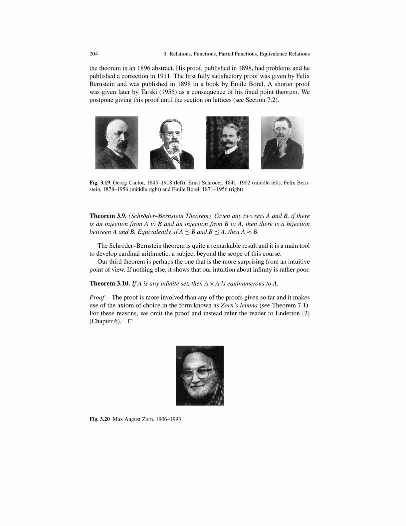
204 3 Relations, Functions, Partial Functions, Equivalence Relations
the theorem in an 1896 abstract. His proof, published in 1898, had problems and hepublished a correction in 1911. The first fully satisfactory proof was given by FelixBernstein and was published in 1898 in a book by Emile Borel. A shorter proofwas given later by Tarski (1955) as a consequence of his fixed point theorem. Wepostpone giving this proof until the section on lattices (see Section 7.2).
Fig. 3.19 Georg Cantor, 1845–1918 (left), Ernst Schroder, 1841–1902 (middle left), Felix Bern-stein, 1878–1956 (middle right) and Emile Borel, 1871–1956 (right)
Theorem 3.9. (Schroder–Bernstein Theorem) Given any two sets A and B, if thereis an injection from A to B and an injection from B to A, then there is a bijectionbetween A and B. Equivalently, if A B and B A, then A≈ B.
The Schroder–Bernstein theorem is quite a remarkable result and it is a main toolto develop cardinal arithmetic, a subject beyond the scope of this course.
Our third theorem is perhaps the one that is the more surprising from an intuitivepoint of view. If nothing else, it shows that our intuition about infinity is rather poor.
Theorem 3.10. If A is any infinite set, then A×A is equinumerous to A.
Proof . The proof is more involved than any of the proofs given so far and it makesuse of the axiom of choice in the form known as Zorn’s lemma (see Theorem 7.1).For these reasons, we omit the proof and instead refer the reader to Enderton [2](Chapter 6). ut
Fig. 3.20 Max August Zorn, 1906–1993
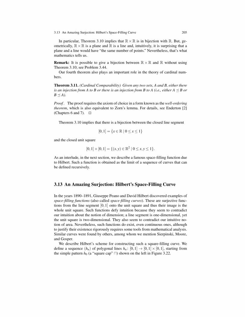
3.13 An Amazing Surjection: Hilbert’s Space-Filling Curve 205
In particular, Theorem 3.10 implies that R×R is in bijection with R. But, ge-ometrically, R×R is a plane and R is a line and, intuitively, it is surprising that aplane and a line would have “the same number of points.” Nevertheless, that’s whatmathematics tells us.
Remark: It is possible to give a bijection between R×R and R without usingTheorem 3.10; see Problem 3.44.
Our fourth theorem also plays an important role in the theory of cardinal num-bers.
Theorem 3.11. (Cardinal Comparability) Given any two sets, A and B, either thereis an injection from A to B or there is an injection from B to A (i.e., either A B orB A).
Proof . The proof requires the axiom of choice in a form known as the well-orderingtheorem, which is also equivalent to Zorn’s lemma. For details, see Enderton [2](Chapters 6 and 7). ut
Theorem 3.10 implies that there is a bijection between the closed line segment
[0,1] = x ∈ R | 0≤ x≤ 1
and the closed unit square
[0,1]× [0,1] = (x,y) ∈ R2 | 0≤ x,y≤ 1.
As an interlude, in the next section, we describe a famous space-filling function dueto Hilbert. Such a function is obtained as the limit of a sequence of curves that canbe defined recursively.
3.13 An Amazing Surjection: Hilbert’s Space-Filling Curve
In the years 1890–1891, Giuseppe Peano and David Hilbert discovered examples ofspace-filling functions (also called space-filling curves). These are surjective func-tions from the line segment [0,1] onto the unit square and thus their image is thewhole unit square. Such functions defy intuition because they seem to contradictour intuition about the notion of dimension; a line segment is one-dimensional, yetthe unit square is two-dimensional. They also seem to contradict our intuitive no-tion of area. Nevertheless, such functions do exist, even continuous ones, althoughto justify their existence rigorously requires some tools from mathematical analysis.Similar curves were found by others, among whom we mention Sierpinski, Moore,and Gosper.
We describe Hilbert’s scheme for constructing such a square-filling curve. Wedefine a sequence (hn) of polygonal lines hn : [0,1]→ [0,1]× [0,1], starting fromthe simple pattern h0 (a “square cap” u) shown on the left in Figure 3.22.
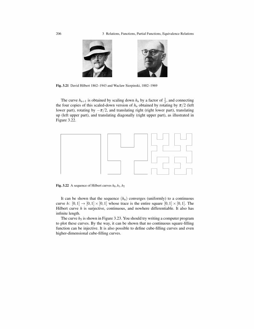
206 3 Relations, Functions, Partial Functions, Equivalence Relations
Fig. 3.21 David Hilbert 1862–1943 and Waclaw Sierpinski, 1882–1969
The curve hn+1 is obtained by scaling down hn by a factor of 12 , and connecting
the four copies of this scaled-down version of hn obtained by rotating by π/2 (leftlower part), rotating by −π/2, and translating right (right lower part), translatingup (left upper part), and translating diagonally (right upper part), as illustrated inFigure 3.22.
Fig. 3.22 A sequence of Hilbert curves h0,h1,h2
It can be shown that the sequence (hn) converges (uniformly) to a continuouscurve h : [0,1]→ [0,1]× [0,1] whose trace is the entire square [0,1]× [0,1]. TheHilbert curve h is surjective, continuous, and nowhere differentiable. It also hasinfinite length.
The curve h5 is shown in Figure 3.23. You should try writing a computer programto plot these curves. By the way, it can be shown that no continuous square-fillingfunction can be injective. It is also possible to define cube-filling curves and evenhigher-dimensional cube-filling curves.
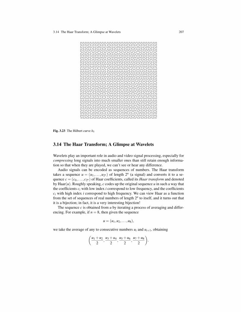
3.14 The Haar Transform; A Glimpse at Wavelets 207
Fig. 3.23 The Hilbert curve h5
3.14 The Haar Transform; A Glimpse at Wavelets
Wavelets play an important role in audio and video signal processing, especially forcompressing long signals into much smaller ones than still retain enough informa-tion so that when they are played, we can’t see or hear any difference.
Audio signals can be encoded as sequences of numbers. The Haar transformtakes a sequence u = (u1, . . . ,u2n) of length 2n (a signal) and converts it to a se-quence c = (c0, . . . ,c2n) of Haar coefficients, called its Haar transform and denotedby Haar(u). Roughly speaking, c codes up the original sequence u in such a way thatthe coefficients ci with low index i correspond to low frequency, and the coefficientsci with high index i correspond to high frequency. We can view Haar as a functionfrom the set of sequences of real numbers of length 2n to itself, and it turns out thatit is a bijection; in fact, it is a very interesting bijection!
The sequence c is obtained from u by iterating a process of averaging and differ-encing. For example, if n = 8, then given the sequence
u = (u1,u2, . . . ,u8),
we take the average of any to consecutive numbers ui and ui+1, obtaining(u1 +u2
2,
u3 +u4
2,
u5 +u6
2,
u7 +u8
2
).

208 3 Relations, Functions, Partial Functions, Equivalence Relations
We can’t recover the original signal from the above sequence, since it consists ofonly 4 numbers, but if we also compute half differences, then we can recover u; thisis because for any two real numbers a,b, we have
a =a+b
2+
a−b2
b =a+b
2− a−b
2.
Using averaging and differencing, we obtain the sequence(u1 +u2
2,
u3 +u4
2,
u5 +u6
2,
u7 +u8
2,
u1−u2
2,
u3−u4
2,
u5−u6
2,
u7−u8
2
).
Then, u1 is recovered by adding up the first element (u1+u2)/2 and the fifth element(u1− u2)/2, u2 is recovered by subtracting the fifth element (u1− u2)/2 from thefirst element (u1 + u2)/2, then u3 is recovered by adding up the second element(u3 + u4)/2 and the sixth element (u3− u4)/2, u4 is recovered by subtracting thesixth element (u3−u4)/2 from the second element (u3 +u4)/2, u5 is recovered byadding up the third element (u5 + u6)/2 and the seventh element (u5− u6)/2, u6is recovered by subtracting the seventh element (u5−u6)/2 from the third element(u5+u6)/2; finally, u7 is recovered by adding up the fourth element (u7+u8)/2 andthe eigth element (u7−u8)/2, and u8 is recovered by subtracting the eigth element(u7−u8)/2 from the fourth element (u7 +u8)/2.
The genius of the Haar transform it to apply the same process recursively to thehalf sequence on the left (and leave the half sequence on the right untouched!).
For simplicity, let us illustrate this process on a sequence of length 4, say
u = (6,4,5,1).
We have the following sequence of steps:
c2 = (6,4,5,1)
c1 = (5,3,1,2)
c0 = (4,1,1,2),
where the numbers in red are obtained by averaging. The Haar transform of u ifc = c0, namely
c = (4,1,1,2).
Note that the first coefficient 4, is the average of the signal u. Then, c2 gives coarsedetails of u, and c3 gives the details in the first part of u, and c4 gives the details ofthe second half of u. The Haar transform performs a multiresolution analysis.
Let us now consider an example with n = 8, say
u = (31,29,23,17,−6,−8,−2,−4).

3.14 The Haar Transform; A Glimpse at Wavelets 209
We get the sequence
c3 = (31,29,23,17,−6,−8,−2,−4)
c2 = (30,20,−7,−3,1,3,1,1)
c1 = (25,−5,5,−2,1,3,1,1)
c0 = (10,15,5,−2,1,3,1,1),
where the numbers in red are obtained by averaging, so
c = (10,15,5,−2,1,3,1,1).
In general, If u is a vector of dimension 2n, we compute the sequence of vectorscn,cn−1, . . . ,c0 as follows: initialize cn as
cn = u,
and for j = n−1, . . . ,0,
for i = 1, . . . ,2 j, do
c j = c j+1
c j(i) = (c j+1(2i−1)+ c j+1(2i))/2
c j(2 j + i) = (c j+1(2i−1)− c j+1(2i))/2.
The Haar transform c = Haar(u) is given by c = c0.Now, given any two real numbers a,b, if we write
m =a+b
2
d =a−b
2,
then we have
a = m+d
b = m−d.
Using these facts, we leave it as an exercise to prove that the inverse of the Haartransform is computed using the following algorithm. If c is a sequence of Haar co-efficients of length 2n, we compute the sequence of vectors u0,u1, . . ., un as follows:initialize u0 as
u0 = c,
and for j = 0, . . . ,n−1,
for i = 1, . . . ,2 j, do

210 3 Relations, Functions, Partial Functions, Equivalence Relations
u j+1 = u j
u j+1(2i−1) = u j(i)+u j(2 j + i)
u j+1(2i) = u j(i)−u j(2 j + i).
The reconstructed signal u = Haar−1(c) is given by u = un.For example, given
c = (10,15,5,−2,1,3,1,1),
we get the sequence
u0 = (10,15,5,−2,1,3,1,1),
u1 = (25,−5,5,−2,1,3,1,1)
u2 = (30,20,−7,−3,1,3,1,1)
u3 = (31,29,23,17,−6,−8,−2,−4),
which gives back u = (31,29,23,17,−6,−8,−2,−4).A nice feature of the Haar decoding algorithm is that is proceed from left to right
(from inside out), so if we send an encoded signal c = (c1, . . . ,c2n), the receivercan start decoding the sequence as soon as it starts receiving the number c1,c2, . . .,without having to wait for the entire sequence to be received.
The Haar transform and its inverse are linear transformations. This means thatc = Haar(v) and u = Haar−1(c) are defined by matrices. For example, if n = 8, theinverse transform Haar−1 is specified by the matrix
W8 =
1 1 1 0 1 0 0 01 1 1 0 −1 0 0 01 1 −1 0 0 1 0 01 1 −1 0 0 −1 0 01 −1 0 1 0 0 1 01 −1 0 1 0 0 −1 01 −1 0 −1 0 0 0 11 −1 0 −1 0 0 0 −1
,
in the sense thatu =W8c,
where u and c are viewed as column vectors. The columns of this matrix are orthog-onal and it is easy to see that
W−18 = diag(1/8,1/8,1/4,1/4,1/2,1/2,1/2,1/2)W>8 .
The columns of the matrix W8 form a basis of orthogonal vectors in R8 known asthe Haar basis.
A pattern is beginning to emerge. It looks like the second Haar basis vector w2is the “mother” of all the other basis vectors, except the first, whose purpose is to
3.14 The Haar Transform; A Glimpse at Wavelets 211
perform averaging. Indeed, in general, given
w2 = (1, . . . ,1,−1, . . . ,−1)︸ ︷︷ ︸2n
,
the other Haar basis vectors are obtained by a “scaling and shifting process.” Startingfrom w2, the scaling process generates the vectors
w3,w5,w9, . . . ,w2 j+1, . . . ,w2n−1+1,
such that w2 j+1+1 is obtained from w2 j+1 by forming two consecutive blocks of 1and −1 of half the size of the blocks in w2 j+1, and setting all other entries to zero.Observe that w2 j+1 has 2 j blocks of 2n− j elements. The shifting process, consistsin shifting the blocks of 1 and −1 in w2 j+1 to the right by inserting a block of(k−1)2n− j zeros from the left, with 0≤ j ≤ n−1 and 1≤ k ≤ 2 j.
It is more convenient if we change our indexing slightly by letting k vary from 0to 2 j−1 and using the index j instead of 2 j. In this case, the Haar basis is denotedby
w1,h00,h
10,h
11,h
20,h
21,h
22,h
23, . . . ,h
jk, . . . ,h
n−12n−1−1.
It turns out that there is a way to understand the Haar basis better if we interpreta sequence u = (u1, . . . ,um) as a piecewise linear function over the interval [0,1).We define the function plf(u) such that
plf(u)(x) = ui,i−1
m≤ x <
im, 1≤ i≤ m.
In words, the function plf(u) has the value u1 on the interval [0,1/m), the value u2on [1/m,2/m), etc., and the value um on the interval [(m−1)/m,1).
For example, the piecewise linear function associated with the vector
u = (2.4,2.2,2.15,2.05,6.8,2.8,−1.1,−1.3)
is shown in Figure 3.24.Then, each basis vector h j
k corresponds to the function
ψj
k = plf(h jk).
In particular, for all n, the Haar basis vectors
h00 = w2 = (1, . . . ,1,−1, . . . ,−1)︸ ︷︷ ︸
2n
yield the same piecewise linear function ψ given by
ψ(x) =
1 if 0≤ x < 1/2−1 if 1/2≤ x < 10 otherwise,

212 3 Relations, Functions, Partial Functions, Equivalence Relations
0 0.1 0.2 0.3 0.4 0.5 0.6 0.7 0.8 0.9 1−2
−1
0
1
2
3
4
5
6
7
Fig. 3.24 The piecewise linear function plf(u)
whose graph is shown in Figure 3.25.
1
1
!1
0
Fig. 3.25 The Haar wavelet ψ
Then, it is easy to see that ψj
k is given by the simple expression
ψj
k (x) = ψ(2 jx− k), 0≤ j ≤ n−1, 0≤ k ≤ 2 j−1.
The above formula makes it clear that ψj
k is obtained from ψ by scaling and shifting.The function φ 0
0 = plf(w1) is the piecewise linear function with the constant value 1on [0,1), and the functions ψ
jk together with φ 0
0 are known as the Haar wavelets.An important and attractive feature of the Haar basis is that it provides a mul-
tiresolution analysis of a signal. Indeed, given a signal u, if c = (c1, . . . ,c2n) is thevector of its Haar coefficients, the coefficients with low index give coarse informa-tion about u, and the coefficients with high index represent fine information. Forexample, if u is an audio signal corresponding to a Mozart concerto played by anorchestra, c1 corresponds to the “background noise,” c2 to the bass, c3 to the firstcello, c4 to the second cello, c5,c6,c7,c7 to the violas, then the violins, etc. This
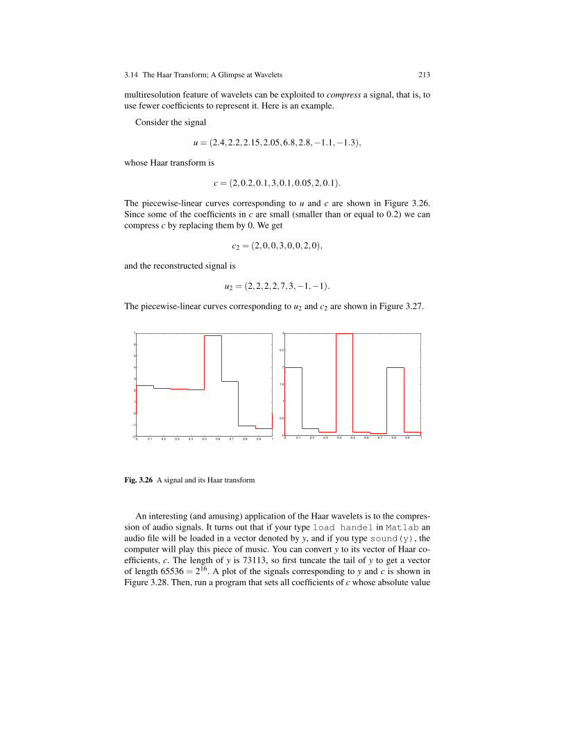
3.14 The Haar Transform; A Glimpse at Wavelets 213
multiresolution feature of wavelets can be exploited to compress a signal, that is, touse fewer coefficients to represent it. Here is an example.
Consider the signal
u = (2.4,2.2,2.15,2.05,6.8,2.8,−1.1,−1.3),
whose Haar transform is
c = (2,0.2,0.1,3,0.1,0.05,2,0.1).
The piecewise-linear curves corresponding to u and c are shown in Figure 3.26.Since some of the coefficients in c are small (smaller than or equal to 0.2) we cancompress c by replacing them by 0. We get
c2 = (2,0,0,3,0,0,2,0),
and the reconstructed signal is
u2 = (2,2,2,2,7,3,−1,−1).
The piecewise-linear curves corresponding to u2 and c2 are shown in Figure 3.27.
0 0.1 0.2 0.3 0.4 0.5 0.6 0.7 0.8 0.9 1−2
−1
0
1
2
3
4
5
6
7
0 0.1 0.2 0.3 0.4 0.5 0.6 0.7 0.8 0.9 10
0.5
1
1.5
2
2.5
3
Fig. 3.26 A signal and its Haar transform
An interesting (and amusing) application of the Haar wavelets is to the compres-sion of audio signals. It turns out that if your type load handel in Matlab anaudio file will be loaded in a vector denoted by y, and if you type sound(y), thecomputer will play this piece of music. You can convert y to its vector of Haar co-efficients, c. The length of y is 73113, so first tuncate the tail of y to get a vectorof length 65536 = 216. A plot of the signals corresponding to y and c is shown inFigure 3.28. Then, run a program that sets all coefficients of c whose absolute value
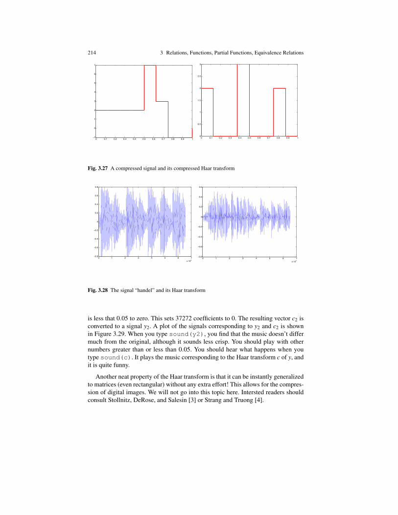
214 3 Relations, Functions, Partial Functions, Equivalence Relations
0 0.1 0.2 0.3 0.4 0.5 0.6 0.7 0.8 0.9 1−1
0
1
2
3
4
5
6
7
0 0.1 0.2 0.3 0.4 0.5 0.6 0.7 0.8 0.9 10
0.5
1
1.5
2
2.5
3
Fig. 3.27 A compressed signal and its compressed Haar transform
0 1 2 3 4 5 6 7x 10⁴
−0.8
−0.6
−0.4
−0.2
0
0.2
0.4
0.6
0.8
0 1 2 3 4 5 6 7x 10⁴
−0.8
−0.6
−0.4
−0.2
0
0.2
0.4
0.6
Fig. 3.28 The signal “handel” and its Haar transform
is less that 0.05 to zero. This sets 37272 coefficients to 0. The resulting vector c2 isconverted to a signal y2. A plot of the signals corresponding to y2 and c2 is shownin Figure 3.29. When you type sound(y2), you find that the music doesn’t differmuch from the original, although it sounds less crisp. You should play with othernumbers greater than or less than 0.05. You should hear what happens when youtype sound(c). It plays the music corresponding to the Haar transform c of y, andit is quite funny.
Another neat property of the Haar transform is that it can be instantly generalizedto matrices (even rectangular) without any extra effort! This allows for the compres-sion of digital images. We will not go into this topic here. Intersted readers shouldconsult Stollnitz, DeRose, and Salesin [3] or Strang and Truong [4].

3.15 Strings, Multisets, Indexed Families 215
0 1 2 3 4 5 6 7x 10⁴
−1
−0.8
−0.6
−0.4
−0.2
0
0.2
0.4
0.6
0.8
1
0 1 2 3 4 5 6 7x 10⁴
−0.8
−0.6
−0.4
−0.2
0
0.2
0.4
0.6
Fig. 3.29 The compressed signal “handel” and its Haar transform
Before we close this chapter and move on to other kinds of relations, namely,partial orders, we illustrate how the notion of function can be used to define strings,multisets, and indexed families rigorously.
3.15 Strings, Multisets, Indexed Families
Strings play an important role in computer science and linguistics because they arethe basic tokens of which languages are made. In fact, formal language theory takesthe (somewhat crude) view that a language is a set of strings. A string is a finitesequence of letters, for example, “Jean”, “Val”, “Mia”, “math”, “gaga”, “abab”.Usually, we have some alphabet in mind and we form strings using letters from thisalphabet. Strings are not sets; the order of the letters matters: “abab” and “baba” aredifferent strings. What matters is the position of every letter. In the string “aba”, theleftmost “a” is in position 1, “b” is in position 2, and the rightmost “b” is in position3. All this suggests defining strings as certain kinds of functions whose domainsare the sets [n] = 1,2, . . . ,n (with [0] = /0) encountered earlier. Here is the verybeginning of the theory of formal languages.
Definition 3.17. An alphabet Σ is any finite set.
We often write Σ = a1, . . . ,ak. The ai are called the symbols of the alphabet.
Remark: There are a few occasions where we allow infinite alphabets but normallyan alphabet is assumed to be finite.
Examples:Σ = aΣ = a,b,cΣ = 0,1
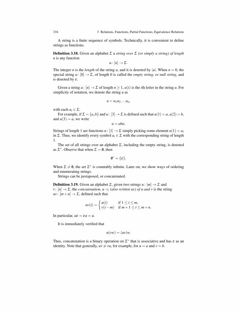
216 3 Relations, Functions, Partial Functions, Equivalence Relations
A string is a finite sequence of symbols. Technically, it is convenient to definestrings as functions.
Definition 3.18. Given an alphabet Σ a string over Σ (or simply a string) of lengthn is any function
u : [n]→ Σ .
The integer n is the length of the string u, and it is denoted by |u|. When n = 0, thespecial string u : [0]→ Σ , of length 0 is called the empty string, or null string, andis denoted by ε .
Given a string u : [n]→ Σ of length n≥ 1, u(i) is the ith letter in the string u. Forsimplicity of notation, we denote the string u as
u = u1u2 . . .un,
with each ui ∈ Σ .For example, if Σ = a,b and u : [3]→Σ is defined such that u(1) = a, u(2) = b,
and u(3) = a, we writeu = aba.
Strings of length 1 are functions u : [1]→ Σ simply picking some element u(1) = aiin Σ . Thus, we identify every symbol ai ∈ Σ with the corresponding string of length1.
The set of all strings over an alphabet Σ , including the empty string, is denotedas Σ ∗. Observe that when Σ = /0, then
/0∗ = ε.
When Σ 6= /0, the set Σ ∗ is countably infinite. Later on, we show ways of orderingand enumerating strings.
Strings can be juxtaposed, or concatenated.
Definition 3.19. Given an alphabet Σ , given two strings u : [m]→ Σ andv : [n]→ Σ , the concatenation, u · v, (also written uv) of u and v is the stringuv : [m+n]→ Σ , defined such that
uv(i) =
u(i) if 1≤ i≤ m,v(i−m) if m+1≤ i≤ m+n.
In particular, uε = εu = u.
It is immediately verified that
u(vw) = (uv)w.
Thus, concatenation is a binary operation on Σ ∗ that is associative and has ε as anidentity. Note that generally, uv 6= vu, for example, for u = a and v = b.
3.15 Strings, Multisets, Indexed Families 217
Definition 3.20. Given an alphabet Σ , given any two strings u,v∈ Σ ∗, we define thefollowing notions as follows.
u is a prefix of v iff there is some y ∈ Σ ∗ such that
v = uy.
u is a suffix of v iff there is some x ∈ Σ ∗ such that
v = xu.
u is a substring of v iff there are some x,y ∈ Σ ∗ such that
v = xuy.
We say that u is a proper prefix (suffix, substring) of v iff u is a prefix (suffix,substring) of v and u 6= v.
For example, ga is a prefix of gallier, the string lier is a suffix of gallier, and allis a substring of gallier.
Finally, languages are defined as follows.
Definition 3.21. Given an alphabet Σ , a language over Σ (or simply a language) isany subset L of Σ ∗.
The next step would be to introduce various formalisms to define languages, suchas automata or grammars but you’ll have to take another course to learn about thesethings.
We now consider multisets. We already encountered multisets in Section 2.2when we defined the axioms of propositional logic. As for sets, in a multiset, theorder of elements does not matter, but as in strings, multiple occurrences of ele-ments matter. For example,
a,a,b,c,c,cis a multiset with two occurrences of a, one occurrence of b, and three occurrencesof c. This suggests defining a multiset as a function with range N, to specify themultiplicity of each element.
Definition 3.22. Given any set S a multiset M over S is any function M : S→ N.A finite multiset M over S is any function M : S→ N such that M(a) 6= 0 only forfinitely many a ∈ S. If M(a) = k > 0, we say that a appears with mutiplicity k in M.
For example, if S = a,b,c, we may use the notation a,a,a,b,c,c for themultiset where a has multiplicity 3, b has multiplicity 1, and c has multiplicity 2.
The empty multiset is the function having the constant value 0. The cardinality|M| of a (finite) multiset is the number
|M|= ∑a∈S
M(a).
218 3 Relations, Functions, Partial Functions, Equivalence Relations
Note that this is well defined because M(a) = 0 for all but finitely many a ∈ S. Forexample,
|a,a,a,b,c,c|= 6.
We can define the union of multisets as follows. If M1 and M2 are two multisets,then M1∪M2 is the multiset given by
(M1∪M2)(a) = M1(a)+M2(a), for all a ∈ S.
A multiset M1 is a submultiset of a multiset M2 if M1(a)≤M2(a) for all a ∈ S. Thedifference of M1 and M2 is the multiset M1−M2 given by
(M1−M2)(a) =
M1(a)−M2(a) if M1(a)≥M2(a)0 if M1(a)< M2(a).
Intersection of multisets can also be defined but we leave this as an exercise.Let us now discuss indexed families. The Cartesian product construct, A1×A2×
·· ·×An, allows us to form finite indexed sequences, 〈a1, . . . ,an〉, but there are situ-ations where we need to have infinite indexed sequences. Typically, we want to beable to consider families of elements indexed by some index set of our choice, sayI. We can do this as follows.
Definition 3.23. Given any X and any other set I, called the index set, the set of I-indexed families (or sequences) of elements from X is the set of all functions A : I→X ; such functions are usually denoted A = (Ai)i∈I . When X is a set of sets, each Aiis some set in X and we call (Ai)i∈I a family of sets (indexed by I).
Observe that if I = [n] = 1, . . . ,n, then an I-indexed family is just a string overX . When I = N, an N-indexed family is called an infinite sequence or often just asequence. In this case, we usually write (xn) for such a sequence ((xn)n∈N, if wewant to be more precise). Also, note that although the notion of indexed family mayseem less general than the notion of arbitrary collection of sets, this is an illusion.Indeed, given any collection of sets X , we may choose the index set I to be X itself,in which case X appears as the range of the identity function, id : X → X .
The point of indexed families is that the operations of union and intersection canbe generalized in an interesting way. We can also form infinite Cartesian products,which are very useful in algebra and geometry.
Given any indexed family of sets (Ai)i∈I , the union of the family (Ai)i∈I , denoted⋃i∈I Ai, is simply the union of the range of A; that is,⋃
i∈I
Ai =⋃
range(A) = a | (∃i ∈ I), a ∈ Ai.
Observe that when I = /0, the union of the family is the empty set. When I 6= /0, wesay that we have a nonempty family (even though some of the Ai may be empty).
Similarly, if I 6= /0, then the intersection of the family (Ai)i∈I , denoted⋂
i∈I Ai, issimply the intersection of the range of A; that is,
3.16 Summary 219⋂i∈I
Ai =⋂
range(A) = a | (∀i ∈ I), a ∈ Ai.
Unlike the situation for union, when I = /0, the intersection of the family does notexist. It would be the set of all sets, which does not exist.
It is easy to see that the laws for union, intersection, and complementation gen-eralize to families but we leave this to the exercises.
An important construct generalizing the notion of finite Cartesian product is theproduct of families.
Definition 3.24. Given any family of sets (Ai)i∈I , the product of the family (Ai)i∈I ,denoted ∏i∈I Ai, is the set
∏i∈I
Ai = a : I→⋃i∈I
Ai | (∀i ∈ I), a(i) ∈ Ai.
Definition 3.24 says that the elements of the product ∏i∈I Ai are the functionsa : I→⋃
i∈I Ai, such that a(i)∈ Ai for every i∈ I. We denote the members of ∏i∈I Aiby (ai)i∈I and we usually call them I-tuples. When I = 1, . . . ,n= [n], the membersof ∏i∈[n] Ai are the functions whose graph consists of the sets of pairs
〈1,a1〉,〈2,a2〉, . . . ,〈n,an〉, ai ∈ Ai, 1≤ i≤ n,
and we see that the function
〈1,a1〉,〈2,a2〉, . . . ,〈n,an〉 7→ 〈a1, . . . ,an〉
yields a bijection between ∏i∈[n] Ai and the Cartesian product A1×·· ·×An. Thus, ifeach Ai is nonempty, the product ∏i∈[n] Ai is nonempty. But what if I is infinite?
If I is infinite, we smell choice functions. That is, an element of ∏i∈I Ai is ob-tained by choosing for every i ∈ I some ai ∈ Ai. Indeed, the axiom of choice isneeded to ensure that ∏i∈I Ai 6= /0 if Ai 6= /0 for all i ∈ I. For the record, we state thisversion (among many) of the axiom of choice.
Axiom of Choice (Product Version)For any family of sets, (Ai)i∈I , if I 6= /0 and Ai 6= /0 for all i ∈ I, then ∏i∈I Ai 6= /0.
Given the product of a family of sets, ∏i∈I Ai, for each i∈ I, we have the functionpri : ∏i∈I Ai→ Ai, called the ith projection function, defined by
pri((ai)i∈I) = ai.
3.16 Summary
This chapter deals with the notions of relations, partial functions and functions,equivalence relations, and their basic properties. The notion of a function is usedto define the concept of a finite set and to compare the “size” of infinite sets. In

220 3 Relations, Functions, Partial Functions, Equivalence Relations
particular, we prove that the power set 2A of any set A is always “strictly bigger”than A itself (Cantor’s theorem).
• We give some examples of functions, emphasizing that a function has a set ofinput values and a set of output values but that a function may not be defined forall of its input values (it may be a partial function). A function is given by a setof 〈 input, output 〉 pairs.
• We define ordered pairs and the Cartesian product A×B of two sets A and B.• We define the first and second projection of a pair.• We define binary relations and their domain and range.• We define the identity relation.• We define functional relations.• We define partial functions, total functions, the graph of a partial or total func-
tion, the domain, and the range of a (partial) function.• We define the preimage or inverse image f−1(a) of an element a by a (partial)
function f .• The set of all functions from A to B is denoted BA.• We revisit the induction principle for N stated in terms of properties and give
several examples of proofs by induction.• We state the complete induction principle for N and prove its validity; we prove
a property of the Fibonacci numbers by complete induction.• We define the composition RS of two relations R and S.• We prove some basic properties of the composition of functional relations.• We define the composition g f of two (partial or total) functions, f and g.• We describe the process of defining functions on N by recursion and state a
basic result about the validity of such a process (The recursion theorem on N).• We define the left inverse and the right inverse of a function.• We define invertible functions and prove the uniqueness of the inverse f−1 of a
function f when it exists.• We define the inverse or converse of a relation .• We define, injective, surjective, and bijective functions.• We characterize injectivity, surjectivity, and bijectivity in terms of left and right
inverses.• We observe that to prove that a surjective function has a right inverse, we need
the axiom of choice (AC).• We define sections, retractions, and the restriction of a function to a subset of
its domain.• We define direct and inverse images of a set under a function ( f (A), respectively,
f−1(B)).• We prove some basic properties of direct and inverse images with respect to
union, intersection, and relative complement.• We define equivalence relations, equivalence classes, quotient sets, and the
canonical projection.• We define partitions and blocks of a partition.• We define a bijection between equivalence relations and partitions (on the same
set).

3.16 Problems 221
• We define when an equivalence relation is a refinement of another equivalencerelation.
• We define the reflexive closure, the transitive closure, and the reflexive and tran-sitive closure of a relation.
• We characterize the smallest equivalence relation containing a relation.• We define when two sets are equinumerous or when a set A dominates a set B.• We give a bijection between N×N and N.• We define when a set if finite or infinite.• We prove that N is not equinumerous to R (the real numbers), a result due to
Cantor, and that there is no surjection from A to 2A.• We define the characteristic function χA of a subset A.• We state and prove the pigeonhole principle.• As an illustration of the pigeonhole principle, we discuss the coin problem of
Frobenius and define the Frobenius number.• We also present a theorem of Erdos and Szekeres about increasing or decreasing
subsequences.• We state the generalized pigeonhole principle.• The set of natural numbers N is infinite.• Every finite set A is equinumerous with a unique set [n] = 1, . . . ,n and the
integer n is called the cardinality of A and is denoted |A|.• If A is a finite set, then for every function f : A→ B the image f (A) of f is finite
and | f (A)| ≤ |A|.• Any subset A of a finite set B is also finite and |A| ≤ |B|.• If A is a finite set, then every injection f : A→ A is a bijection and every surjec-
tion f : A→ A is a bijection.• A set A is countable iff there is a surjection from N onto A.• For every infinite set A there is an injection from N into A.• A set A is infinite iff it is equinumerous to a proper subset of itself.• We state the Schroder–Bernstein theorem.• We state that every infinite set A is equinumerous to A×A.• We state the cardinal comparability theorem.• We mention Zorn’s lemma, one of the many versions of the axiom of choice.• We describe Hilbert’s space-filling curve.• We describe the Haar transform as an example of a bijection on sequences of
length 2n that has applications to compression in signal processing.• We define strings and multisets.• We define the product of a family of sets and explain how the non-emptyness of
such a product is equivalent to the axiom of choice.
Problems
3.1. Given any two sets A,B, prove that for all a1,a2 ∈ A and all b1,b2 ∈ B,
222 3 Relations, Functions, Partial Functions, Equivalence Relations
a1,a1,b1= a2,a2,b2
iffa1 = a2 and b1 = b2.
3.2. (a) Prove that the composition of two injective functions is injective. Prove thatthe composition of two surjective functions is surjective.
(b) Prove that a function f : A→ B is injective iff for all functions g,h : C→ A,
if f g = f h, then g = h.
(c) Prove that a function f : A→ B is surjective iff for all functions g,h : B→C,
if g f = h f , then g = h.
3.3. (a) Prove thatn
∑k=1
k2 =n(n+1)(2n+1)
6.
(b) Prove thatn
∑k=1
k3 =
(n
∑k=1
k
)2
.
3.4. Given any finite set A, let |A| denote the number of elements in A.(a) If A and B are finite sets, prove that
|A∪B|= |A|+ |B|− |A∩B|.
(b) If A, B, and C are finite sets, prove that
|A∪B∪C|= |A|+ |B|+ |C|− |A∩B|− |A∩C|− |B∩C|+ |A∩B∩C|.
3.5. Prove that there is no set X such that
2X ⊆ X .
Hint. Given any two sets A,B, if there is an injection from A to B, then there is asurjection from B to A.
3.6. Let f : X → Y be any function. (a) Prove that for any two subsets A,B⊆ X wehave
f (A∪B) = f (A)∪ f (B)
f (A∩B) ⊆ f (A)∩ f (B).
Give an example of a function f and of two subsets A,B such that
3.16 Problems 223
f (A∩B) 6= f (A)∩ f (B).
Prove that if f : X → Y is injective, then
f (A∩B) = f (A)∩ f (B).
(b) For any two subsets C,D⊆ Y , prove that
f−1(C∪D) = f−1(C)∪ f−1(D)
f−1(C∩D) = f−1(C)∩ f−1(D).
(c) Prove that for any two subsets A⊆ X and C ⊆ Y , we have
f (A)⊆C iff A⊆ f−1(C).
3.7. Let R and S be two relations on a set X . (1) Prove that if R and S are bothreflexive, then RS is reflexive.
(2) Prove that if R and S are both symmetric and if R S = S R, then R S issymmetric.
(3) Prove that if R and S are both transitive and if R S = S R, then R S istransitive.
Can the hypothesis RS = SR be omitted?(4) Prove that if R and S are both equivalence relations and if RS = S R, then
RS is the smallest equivalence relation containing R and S.
3.8. Prove Proposition 3.7.
3.9. Prove that the set of natural numbers N is infinite. (Recall, a set X is finite iffthere is a bijection from X to [n] = 1, . . . ,n, where n ∈N is a natural number with[0] = /0. Thus, a set X is infinite iff there is no bijection from X to any [n], withn ∈ N.)
3.10. Let R⊆ A×A be a relation. Prove that if RR = idA, then R is the graph of abijection whose inverse is equal to itself.
3.11. Given any three relations R ⊆ A×B, S ⊆ B×C, and T ⊆ C×D, prove theassociativity of composition:
(RS)T = R (ST ).
3.12. Let f : A→ A′ and g : B→ B′ be two functions and defineh : A×B→ A′×B′ by
h(〈a,b〉) = 〈 f (a),g(b)〉,for all a ∈ A and b ∈ B.
(a) Prove that if f and g are injective, then so is h.
Hint. Use the definition of injectivity, not the existence of a left inverse and do notproceed by contradiction.

224 3 Relations, Functions, Partial Functions, Equivalence Relations
(b) Prove that if f and g are surjective, then so is h.
Hint. Use the definition of surjectivity, not the existence of a right inverse and donot proceed by contradiction.
3.13. Let f : A→ A′ and g : B→ B′ be two injections. Prove that ifIm f ∩ Img = /0, then there is an injection from A∪B to A′∪B′.
Is the above still correct if Im f ∩ Img 6= /0?
3.14. Let [0,1] and (0,1) denote the set of real numbers
[0,1] = x ∈ R | 0≤ x≤ 1(0,1) = x ∈ R | 0 < x < 1.
(a) Give a bijection f : [0,1]→ (0,1).
Hint. There are such functions that are the identity almost everywhere but for acountably infinite set of points in [0,1].
(b) Consider the open square (0,1)× (0,1) and the closed square [0,1]× [0,1].Give a bijection f : [0,1]× [0,1]→ (0,1)× (0,1).
3.15. Recall that for any function f : A→ A, for every k ∈ N, we define f k : A→ Aby
f 0 = idA
f k+1 = f k f .
Also, an element a ∈ A is a fixed point of f if f (a) = a. Now, assume that π : [n]→[n] is any permutation of the finite set [n] = 1,2, . . . ,n.
(1) For any i ∈ [n], prove that there is a least r with 1≤ r ≤ n such that πr(i) = i.(2) Define the relation Rπ on [n] such that iRπ j iff there is some integer k ≥ 1
such thatj = π
k(i).
Prove that Rπ is an equivalence relation.(3) Prove that every equivalence class of Rπ is either a singleton set i or a set
of the formJ = i,π(i),π2(i), . . . ,πri−1(i),
with ri the least integer such that πri(i) = i and 2≤ ri ≤ n. The equivalence class ofany element i∈ [n] is called the orbit of i (under π). We say that an orbit is nontrivialif it has at least two elements.
(4) A k-cycle (or cyclic permutation of order k) is a permutation σ : [n]→ [n]such that for some sequence (i1, i2, . . . , ik) of distinct elements of [n] with 2≤ k≤ n,
σ(i1) = i2,σ(i2) = i3, . . . ,σ(ik−1) = ik,σ(ik) = i1
and σ( j) = j for all j ∈ [n]−i1, . . . , ik. The set i1, i2, . . . , ik is called the domainof the cyclic permutation. Observe that any element i ∈ [n] is a fixed point of σ iff iis not in the domain of σ .
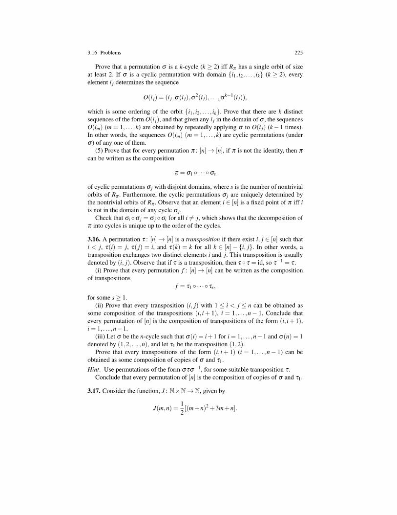
3.16 Problems 225
Prove that a permutation σ is a k-cycle (k ≥ 2) iff Rπ has a single orbit of sizeat least 2. If σ is a cyclic permutation with domain i1, i2, . . . , ik (k ≥ 2), everyelement i j determines the sequence
O(i j) = (i j,σ(i j),σ2(i j), . . . ,σ
k−1(i j)),
which is some ordering of the orbit i1, i2, . . . , ik. Prove that there are k distinctsequences of the form O(i j), and that given any i j in the domain of σ , the sequencesO(im) (m = 1, . . . ,k) are obtained by repeatedly applying σ to O(i j) (k− 1 times).In other words, the sequences O(im) (m = 1, . . . ,k) are cyclic permutations (underσ ) of any one of them.
(5) Prove that for every permutation π : [n]→ [n], if π is not the identity, then π
can be written as the composition
π = σ1 · · · σs
of cyclic permutations σ j with disjoint domains, where s is the number of nontrivialorbits of Rπ . Furthermore, the cyclic permutations σ j are uniquely determined bythe nontrivial orbits of Rπ . Observe that an element i ∈ [n] is a fixed point of π iff iis not in the domain of any cycle σ j.
Check that σi σ j = σ j σi for all i 6= j, which shows that the decomposition ofπ into cycles is unique up to the order of the cycles.
3.16. A permutation τ : [n]→ [n] is a transposition if there exist i, j ∈ [n] such thati < j, τ(i) = j, τ( j) = i, and τ(k) = k for all k ∈ [n]−i, j. In other words, atransposition exchanges two distinct elements i and j. This transposition is usuallydenoted by (i, j). Observe that if τ is a transposition, then τ τ = id, so τ−1 = τ .
(i) Prove that every permutation f : [n]→ [n] can be written as the compositionof transpositions
f = τ1 · · · τs,
for some s≥ 1.(ii) Prove that every transposition (i, j) with 1 ≤ i < j ≤ n can be obtained as
some composition of the transpositions (i, i + 1), i = 1, . . . ,n− 1. Conclude thatevery permutation of [n] is the composition of transpositions of the form (i, i+ 1),i = 1, . . . ,n−1.
(iii) Let σ be the n-cycle such that σ(i) = i+1 for i = 1, . . . ,n−1 and σ(n) = 1denoted by (1,2, . . . ,n), and let τ1 be the transposition (1,2).
Prove that every transpositions of the form (i, i + 1) (i = 1, . . . ,n− 1) can beobtained as some composition of copies of σ and τ1.Hint. Use permutations of the form στσ−1, for some suitable transposition τ .
Conclude that every permutation of [n] is the composition of copies of σ and τ1.
3.17. Consider the function, J : N×N→ N, given by
J(m,n) =12[(m+n)2 +3m+n].

226 3 Relations, Functions, Partial Functions, Equivalence Relations
(a) Prove that for any z ∈ N, if J(m,n) = z, then
8z+1 = (2m+2n+1)2 +8m.
Deduce from the above that
2m+2n+1≤√
8z+1 < 2m+2n+3.
(b) If x 7→ bxc is the function from R to N (the floor function), where bxc is thelargest integer ≤ x (e.g., b2.3c= 2, b
√2c= 1), prove that
b√
8z+1c+1 = 2m+2n+2 or b√
8z+1c+1 = 2m+2n+3,
so thatb(b√
8z+1c+1)/2c= m+n+1.
(c) Because J(m,n) = z means that
2z = (m+n)2 +3m+n,
prove that m and n are solutions of the system
m+n = b(b√
8z+1c+1)/2c−13m+n = 2z− (b(b
√8z+1c+1)/2c−1)2.
If we let
Q1(z) = b(b√
8z+1c+1)/2c−1Q2(z) = 2z− (b(b
√8z+1c+1)/2c−1)2 = 2z− (Q1(z))2,
prove that Q2(z)−Q1(z) is even and that
m =12(Q2(z)−Q1(z)) = K(z)
n = Q1(z)−12(Q2(z)−Q1(z)) = L(z).
Conclude that J is a bijection between N×N and N, with
m = K(J(m,n))
n = L(J(m,n)).
Remark: It can also be shown that J(K(z),L(z)) = z.
3.18. (i) In 3-dimensional space R3 the sphere S2 is the set of points of coordinates(x,y,z) such that x2 + y2 + z2 = 1. The point N = (0,0,1) is called the north pole,and the point S = (0,0,−1) is called the south pole. The stereographic projection

3.16 Problems 227
map σN : (S2−N)→ R2 is defined as follows. For every point M 6= N on S2, thepoint σN(M) is the intersection of the line through N and M and the equatorial planeof equation z = 0.
Prove that if M has coordinates (x,y,z) (with x2 + y2 + z2 = 1), then
σN(M) =
(x
1− z,
y1− z
).
Hint. Recall that if A = (a1,a2,a3) and B = (b1,b2,b3) are any two distinct pointsin R3, then the unique line (AB) passing through A and B has parametric equations
x = (1− t)a1 + tb1
y = (1− t)a2 + tb2
z = (1− t)a3 + tb3,
which means that every point (x,y,z) on the line (AB) is of the above form, witht ∈ R. Find the intersection of a line passing through the North pole and a pointM 6= N on the sphere S2.
Prove that σN is bijective and that its inverse is given by the map τN : R2 →(S2−N) with
(x,y) 7→(
2xx2 + y2 +1
,2y
x2 + y2 +1,
x2 + y2−1x2 + y2 +1
).
Hint. Find the intersection of a line passing through the North pole and some pointP of the equatorial plane z = 0 with the sphere of equation
x2 + y2 + z2 = 1.
Similarly, σS : (S2−S)→ R2 is defined as follows. For every point M 6= S onS2, the point σS(M) is the intersection of the line through S and M and the plane ofequation z = 0.
Prove that
σS(M) =
(x
1+ z,
y1+ z
).
Prove that σS is bijective and that its inverse is given by the map, τS : R2 → (S2−S), with
(x,y) 7→(
2xx2 + y2 +1
,2y
x2 + y2 +1,
1− x2− y2
x2 + y2 +1
).
(ii) Give a bijection between the sphere S2 and the equatorial plane of equationz = 0.
Hint. Use the stereographic projection and the method used in Problem 3.14, todefine a bijection between [0,1] and (0,1).
228 3 Relations, Functions, Partial Functions, Equivalence Relations
3.19. (a) Give an example of a function f : A→ A such that f 2 = f f = f and f isnot the identity function.
(b) Prove that if a function f : A→ A is not the identity function and f 2 = f , thenf is not invertible.
(c) Give an example of an invertible function f : A→A, such that f 3 = f f f =f , yet f f 6= f .
(d) Give an example of a noninvertible function f : A→ A, such that f 3 = f f f = f , yet f f 6= f .
3.20. Finish the proof of Theorem 3.6. That is, prove that for any n≥ (p−1)(q−1),if we consider the sequence
n+q,n, n−q, n−2q, . . . , n− (p−2)q,
then some integer in this sequence is divisible by p with nonnegative quotient, andthat when this number if n+q, then n+q = ph with h≥ q.
Hint. If n≥ (p−1)(q−1), then n+q≥ p(q−1)+1.
3.21. (1) Let (−1,1) be the set of real numbers
(−1,1) = x ∈ R | −1 < x < 1.
Let f : R→ (−1,1) be the function given by
f (x) =x√
1+ x2.
Prove that f is a bijection. Find the inverse of f .(2) Let (0,1) be the set of real numbers
(0,1) = x ∈ R | 0 < x < 1.
Give a bijection between (−1,1) and (0,1). Use (1) and (2) to give a bijectionbetween R and (0,1).
3.22. Let D⊆ R2 be the subset of the real plane given by
D = (x,y) ∈ R2 | x2 + y2 < 1,
that is, all points strictly inside of the unit circle x2+y2 = 1. The set D is often calledthe open unit disc. Let f : R2→ D be the function given by
f (x,y) =
(x√
1+ x2 + y2,
y√1+ x2 + y2
).
(1) Prove that f is a bijection and find its inverse.(2) Give a bijection between the sphere S2 and the open unit disk D in the equa-
torial plane.

3.16 Problems 229
3.23. Prove by induction on n that
n2 ≤ 2n for all n≥ 4.
Hint. You need to show that 2n+1≤ n2 for all n≥ 3.
3.24. Let f : A→ A be a function.(a) Prove that if
f f f = f f and f 6= idA, (∗)then f is neither injective nor surjective.
Hint. Proceed by contradiction and use the characterization of injections and surjec-tions in terms of left and right inverses.
(b) Give a simple example of a function f : a,b,c → a,b,c, satisfying theconditions of (∗).
3.25. Recall that a set A is infinite iff there is no bijection from 1, . . . ,n onto A,for any natural number n ∈ N. Prove that the set of odd natural numbers is infinite.
3.26. Consider the sum
31 ·4 +
54 ·9 + · · ·+ 2n+1
n2 · (n+1)2 ,
with n≥ 1.Which of the following expressions is the sum of the above:
(1)n+2
(n+1)2 (2)n(n+2)(n+1)2 .
Justify your answer.Hint. Note that
n4 +6n3 +12n2 +10n+3 = (n3 +3n2 +3n+1)(n+3).
3.27. Consider the following version of the Fibonacci sequence starting from F0 = 0and defined by:
F0 = 0F1 = 1
Fn+2 = Fn+1 +Fn, n≥ 0.
Prove the following identity, for any fixed k ≥ 1 and all n≥ 0,
Fn+k = FkFn+1 +Fk−1Fn.
3.28. Recall that the triangular numbers ∆n are given by the formula
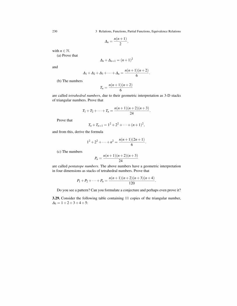
230 3 Relations, Functions, Partial Functions, Equivalence Relations
∆n =n(n+1)
2,
with n ∈ N.(a) Prove that
∆n +∆n+1 = (n+1)2
and
∆1 +∆2 +∆3 + · · ·+∆n =n(n+1)(n+2)
6.
(b) The numbers
Tn =n(n+1)(n+2)
6are called tetrahedral numbers, due to their geometric interpretation as 3-D stacksof triangular numbers. Prove that
T1 +T2 + · · ·+Tn =n(n+1)(n+2)(n+3)
24.
Prove thatTn +Tn+1 = 12 +22 + · · ·+(n+1)2,
and from this, derive the formula
12 +22 + · · ·+n2 =n(n+1)(2n+1)
6.
(c) The numbers
Pn =n(n+1)(n+2)(n+3)
24are called pentatope numbers. The above numbers have a geometric interpretationin four dimensions as stacks of tetrahedral numbers. Prove that
P1 +P2 + · · ·+Pn =n(n+1)(n+2)(n+3)(n+4)
120.
Do you see a pattern? Can you formulate a conjecture and perhaps even prove it?
3.29. Consider the following table containing 11 copies of the triangular number,∆5 = 1+2+3+4+5:
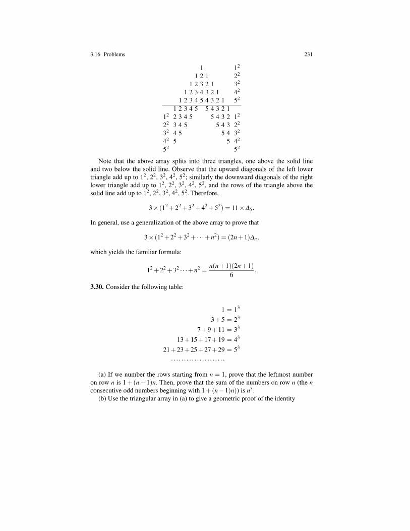
3.16 Problems 231
1 12
1 2 1 22
1 2 3 2 1 32
1 2 3 4 3 2 1 42
1 2 3 4 5 4 3 2 1 52
1 2 3 4 5 5 4 3 2 112 2 3 4 5 5 4 3 2 12
22 3 4 5 5 4 3 22
32 4 5 5 4 32
42 5 5 42
52 52
Note that the above array splits into three triangles, one above the solid lineand two below the solid line. Observe that the upward diagonals of the left lowertriangle add up to 12, 22, 32, 42, 52; similarly the downward diagonals of the rightlower triangle add up to 12, 22, 32, 42, 52, and the rows of the triangle above thesolid line add up to 12, 22, 32, 42, 52. Therefore,
3× (12 +22 +32 +42 +52) = 11×∆5.
In general, use a generalization of the above array to prove that
3× (12 +22 +32 + · · ·+n2) = (2n+1)∆n,
which yields the familiar formula:
12 +22 +32 · · ·+n2 =n(n+1)(2n+1)
6.
3.30. Consider the following table:
1 = 13
3+5 = 23
7+9+11 = 33
13+15+17+19 = 43
21+23+25+27+29 = 53
· · · · · · · · · · · · · · · · · · · · ·
(a) If we number the rows starting from n = 1, prove that the leftmost numberon row n is 1+(n− 1)n. Then, prove that the sum of the numbers on row n (the nconsecutive odd numbers beginning with 1+(n−1)n)) is n3.
(b) Use the triangular array in (a) to give a geometric proof of the identity
232 3 Relations, Functions, Partial Functions, Equivalence Relations
n
∑k=1
k3 =
(n
∑k=1
k
)2
.
Hint. Recall that1+3+ · · ·+2n−1 = n2.
3.31. Let f : A→ B be a function and define the function g : B→ 2A by
g(b) = f−1(b) = a ∈ A | f (a) = b,
for all b ∈ B. (a) Prove that if f is surjective, then g is injective.(b) If g is injective, can we conclue that f is surjective?
3.32. Let X ,Y,Z be any three nonempty sets and let f : X → Y be any function.Define the function R f : ZY → ZX (R f , as a reminder that we compose with f on theright), by
R f (h) = h f ,
for every function h : Y → Z.Let T be another nonempty set and let g : Y → T be any function.(a) Prove that
Rg f = R f Rg
and if X = Y and f = idX , then
RidX (h) = h,
for every function h : X → Z.(b) Use (a) to prove that if f is surjective, then R f is injective and if f is injective,
then R f is surjective.
3.33. Let X ,Y,Z be any three nonempty sets and let g : Y → Z be any function.Define the function Lg : Y X → ZX (Lg, as a reminder that we compose with g on theleft), by
Lg( f ) = g f ,
for every function f : X → Y .(a) Prove that if Y = Z and g = idY , then
LidY ( f ) = f ,
for all f : X → Y .Let T be another nonempty set and let h : Z→ T be any function. Prove that
Lhg = Lh Lg.
(b) Use (a) to prove that if g is injective, then Lg : Y X → ZX is also injective andif g is surjective, then Lg : Y X → ZX is also surjective.
3.16 Problems 233
3.34. Recall that given any two sets X ,Y , every function f : X → Y induces a func-tion f : 2X → 2Y such that for every subset A⊆ X ,
f (A) = f (a) ∈ Y | a ∈ A
and a function f−1 : 2Y → 2X , such that, for every subset B⊆ Y ,
f−1(B) = x ∈ X | f (x) ∈ B.
(a) Prove that if f : X → Y is injective, then so is f : 2X → 2Y .(b) Prove that if f is bijective then f−1( f (A)) = A and f ( f−1(B)) = B, for all
A⊆ X and all B⊆ Y . Deduce from this that f : 2X → 2Y is bijective.(c) Prove that for any set A there is an injection from the set AA of all functions
from A to A to 2A×A, the power set of A×A. If A is infinite, prove that there is aninjection from AA to 2A.
3.35. Recall that given any two sets X ,Y , every function f : X → Y induces a func-tion f : 2X → 2Y such that for every subset A⊆ X ,
f (A) = f (a) ∈ Y | a ∈ A
and a function f−1 : 2Y → 2X , such that, for every subset B⊆ Y ,
f−1(B) = x ∈ X | f (x) ∈ B.
(a) Prove that if f : X → Y is surjective, then so is f : 2X → 2Y .(b) If A is infinite, prove that there is a bijection from AA to 2A.
Hint. Prove that there is an injection from AA to 2A and an injection from 2A to AA.
3.36. (a) Finish the proof of Theorem 3.8, which states that for any infinite set Xthere is an injection from N into X . Use this to prove that there is a bijection betweenX and X×N.
(b) Prove that if a subset A⊆N of N is not finite, then there is a bijection betweenA and N.
(c) Prove that every infinite set X can be written as a disjoint union X =⋃
i∈I Xi,where every Xi is in bijection with N.
(d) If X is any set, finite or infinite, prove that if X has at least two elements thenthere is a bijection f of X leaving no element fixed (i.e., so that f (x) 6= x for allx ∈ X).
3.37. Prove that if (Xi)i∈I is a family of sets and if I and all the Xi are countable,then (Xi)i∈I is also countable.Hint. Define a surjection from N×N onto (Xi)i∈I .
3.38. Consider the alphabet, Σ = a,b. We can enumerate all strings in a,b∗as follows. Say that u precedes v if |u| < |v| and if |u| = |v|, use the lexicographic(dictionary) order. The enumeration begins with
234 3 Relations, Functions, Partial Functions, Equivalence Relations
ε
a, b
aa, ab, ba, bb
aaa, aab, aba, abb, baa, bab, bba, bbb
We would like to define a function, f : a,b∗→ N, such that f (u) is the positionof the string u in the above list, starting with f (ε) = 0. For example,
f (baa) = 11.
(a) Prove that if u = u1 · · ·un (with u j ∈ a,b and n≥ 1), then
f (u) = i12n−1 + i22n−2 + · · ·+ in−121 + in= 2n−1+(i1−1)2n−1 +(i2−1)2n−2 + · · ·+(in−1−1)21 + in−1,
with i j = 1 if u j = a, else i j = 2 if u j = b.(b) Prove that the above function is a bijection f : a,b∗→ N.(c) Consider any alphabet Σ = a1, . . . ,am, with m ≥ 2. We can also list all
strings in Σ ∗ as in (a). Prove that the listing function f : Σ ∗→N is given by f (ε) = 0and if u = ai1 · · ·ain (with ai j ∈ Σ and n≥ 1) by
f (u) = i1mn−1 + i2mn−2 + · · ·+ in−1m1 + in
=mn−1m−1
+(i1−1)mn−1 +(i2−1)mn−2 + · · ·+(in−1−1)m1 + in−1,
Prove that the above function f : Σ ∗→ N is a bijection.(d) Consider any infinite set A and pick two distinct elements, a1,a2, in A. We
would like to define a surjection from AA to 2A by mapping any function f : A→ Ato its image,
Im f = f (a) | a ∈ A.The problem with the above definition is that the empty set is missed. To fix thisproblem, let f0 be the function defined so that f0(a0) = a1 and f0(a) = a0 for alla ∈ A−a0. Then, we define S : AA→ 2A by
S( f ) =
/0 if f = f0Im( f ) if f 6= f0.
Prove that the function S : AA→ 2A is indeed a surjection.(e) Assume that Σ is an infinite set and consider the set of all finite strings Σ ∗. If
Σ n denotes the set of all strings of length n, observe that
Σ∗ =
⋃n≥0
Σn.
Prove that there is a bijection between Σ ∗ and Σ .
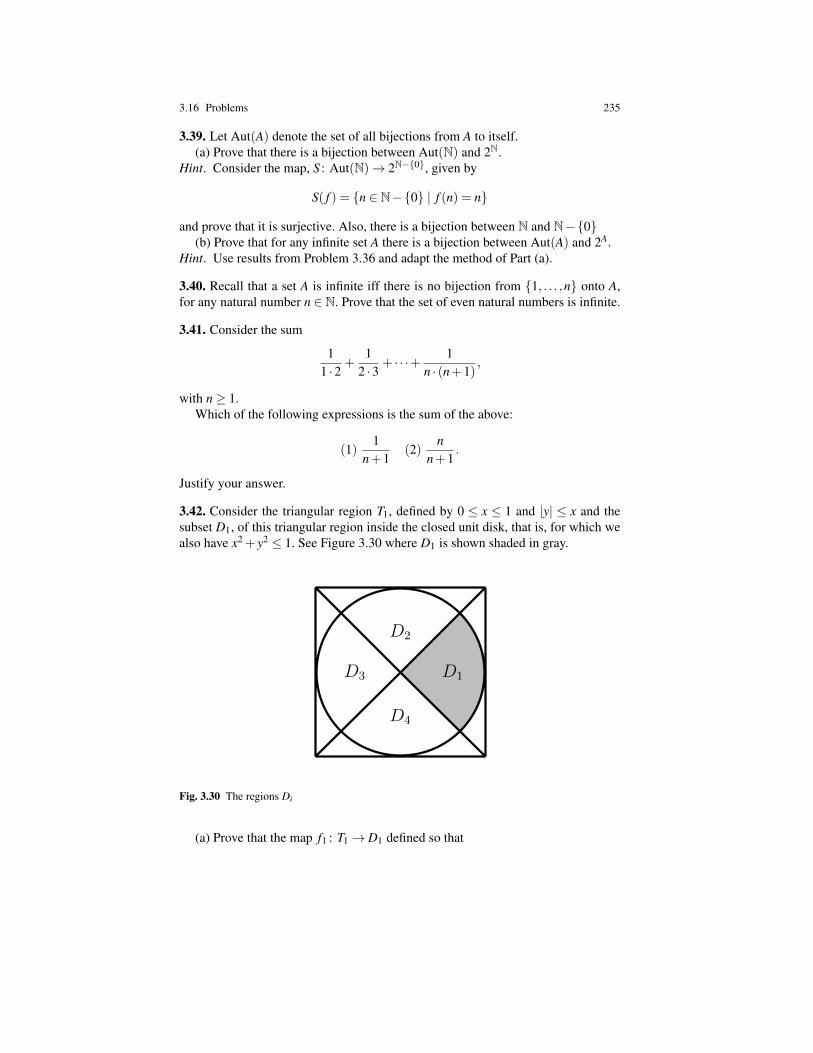
3.16 Problems 235
3.39. Let Aut(A) denote the set of all bijections from A to itself.(a) Prove that there is a bijection between Aut(N) and 2N.
Hint. Consider the map, S : Aut(N)→ 2N−0, given by
S( f ) = n ∈ N−0 | f (n) = n
and prove that it is surjective. Also, there is a bijection between N and N−0(b) Prove that for any infinite set A there is a bijection between Aut(A) and 2A.
Hint. Use results from Problem 3.36 and adapt the method of Part (a).
3.40. Recall that a set A is infinite iff there is no bijection from 1, . . . ,n onto A,for any natural number n ∈ N. Prove that the set of even natural numbers is infinite.
3.41. Consider the sum
11 ·2 +
12 ·3 + · · ·+ 1
n · (n+1),
with n≥ 1.Which of the following expressions is the sum of the above:
(1)1
n+1(2)
nn+1
.
Justify your answer.
3.42. Consider the triangular region T1, defined by 0 ≤ x ≤ 1 and |y| ≤ x and thesubset D1, of this triangular region inside the closed unit disk, that is, for which wealso have x2 + y2 ≤ 1. See Figure 3.30 where D1 is shown shaded in gray.
1
D1D3
D2
D4
Fig. 3.30 The regions Di
(a) Prove that the map f1 : T1→ D1 defined so that
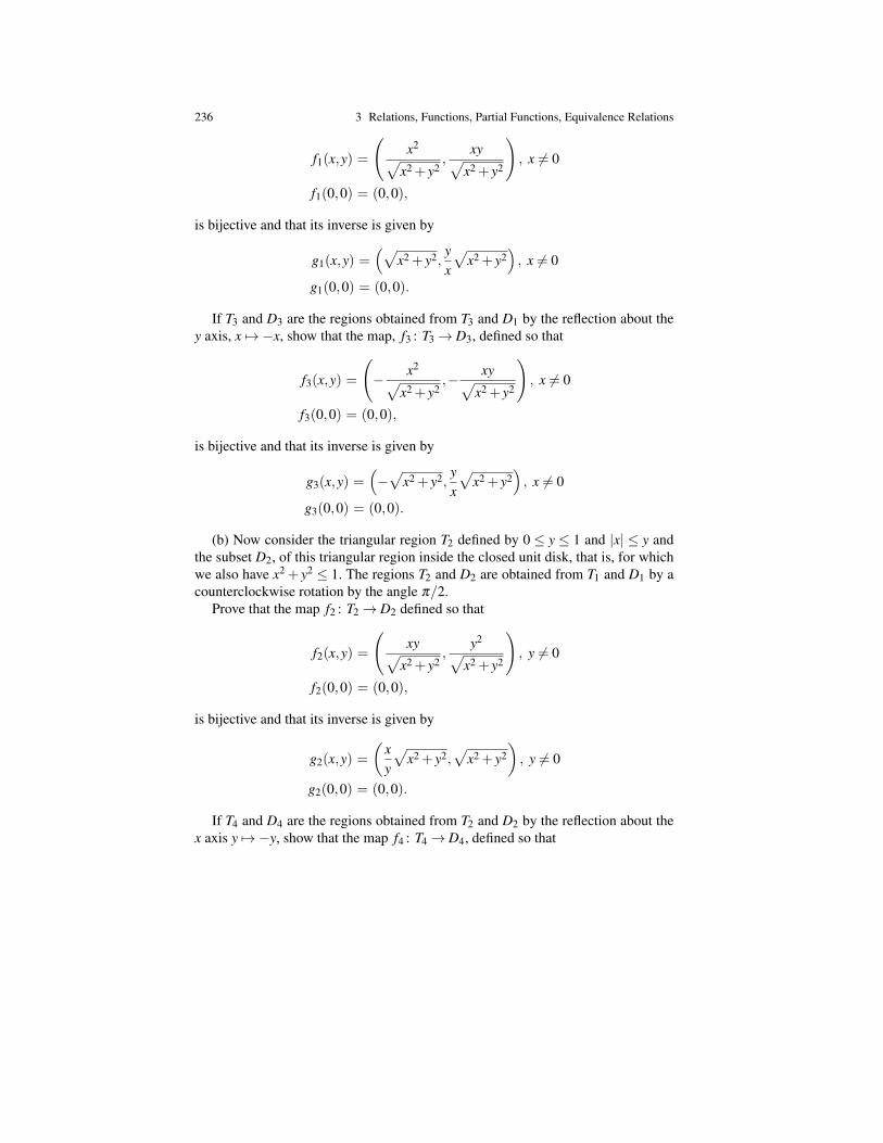
236 3 Relations, Functions, Partial Functions, Equivalence Relations
f1(x,y) =
(x2√
x2 + y2,
xy√x2 + y2
), x 6= 0
f1(0,0) = (0,0),
is bijective and that its inverse is given by
g1(x,y) =(√
x2 + y2,yx
√x2 + y2
), x 6= 0
g1(0,0) = (0,0).
If T3 and D3 are the regions obtained from T3 and D1 by the reflection about they axis, x 7→ −x, show that the map, f3 : T3→ D3, defined so that
f3(x,y) =
(− x2√
x2 + y2,− xy√
x2 + y2
), x 6= 0
f3(0,0) = (0,0),
is bijective and that its inverse is given by
g3(x,y) =(−√
x2 + y2,yx
√x2 + y2
), x 6= 0
g3(0,0) = (0,0).
(b) Now consider the triangular region T2 defined by 0 ≤ y ≤ 1 and |x| ≤ y andthe subset D2, of this triangular region inside the closed unit disk, that is, for whichwe also have x2 + y2 ≤ 1. The regions T2 and D2 are obtained from T1 and D1 by acounterclockwise rotation by the angle π/2.
Prove that the map f2 : T2→ D2 defined so that
f2(x,y) =
(xy√
x2 + y2,
y2√x2 + y2
), y 6= 0
f2(0,0) = (0,0),
is bijective and that its inverse is given by
g2(x,y) =(
xy
√x2 + y2,
√x2 + y2
), y 6= 0
g2(0,0) = (0,0).
If T4 and D4 are the regions obtained from T2 and D2 by the reflection about thex axis y 7→ −y, show that the map f4 : T4→ D4, defined so that
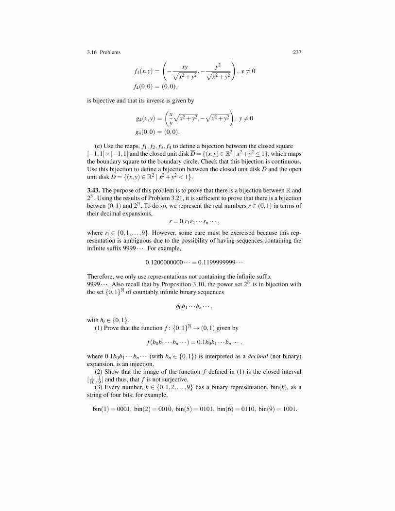
3.16 Problems 237
f4(x,y) =
(− xy√
x2 + y2,− y2√
x2 + y2
), y 6= 0
f4(0,0) = (0,0),
is bijective and that its inverse is given by
g4(x,y) =(
xy
√x2 + y2,−
√x2 + y2
), y 6= 0
g4(0,0) = (0,0).
(c) Use the maps, f1, f2, f3, f4 to define a bijection between the closed square[−1,1]× [−1,1] and the closed unit disk D= (x,y)∈R2 | x2+y2≤ 1, which mapsthe boundary square to the boundary circle. Check that this bijection is continuous.Use this bijection to define a bijection between the closed unit disk D and the openunit disk D = (x,y) ∈ R2 | x2 + y2 < 1.
3.43. The purpose of this problem is to prove that there is a bijection between R and2N. Using the results of Problem 3.21, it is sufficient to prove that there is a bijectionbetwen (0,1) and 2N. To do so, we represent the real numbers r ∈ (0,1) in terms oftheir decimal expansions,
r = 0.r1r2 · · ·rn · · · ,where ri ∈ 0,1, . . . ,9. However, some care must be exercised because this rep-resentation is ambiguous due to the possibility of having sequences containing theinfinite suffix 9999 · · · . For example,
0.1200000000 · · ·= 0.1199999999 · · ·
Therefore, we only use representations not containing the infinite suffix9999 · · · . Also recall that by Proposition 3.10, the power set 2N is in bijection withthe set 0,1N of countably infinite binary sequences
b0b1 · · ·bn · · · ,
with bi ∈ 0,1.(1) Prove that the function f : 0,1N→ (0,1) given by
f (b0b1 · · ·bn · · ·) = 0.1b0b1 · · ·bn · · · ,
where 0.1b0b1 · · ·bn · · · (with bn ∈ 0,1) is interpreted as a decimal (not binary)expansion, is an injection.
(2) Show that the image of the function f defined in (1) is the closed interval[ 1
10 ,19 ] and thus, that f is not surjective.
(3) Every number, k ∈ 0,1,2, . . . ,9 has a binary representation, bin(k), as astring of four bits; for example,
bin(1) = 0001, bin(2) = 0010, bin(5) = 0101, bin(6) = 0110, bin(9) = 1001.
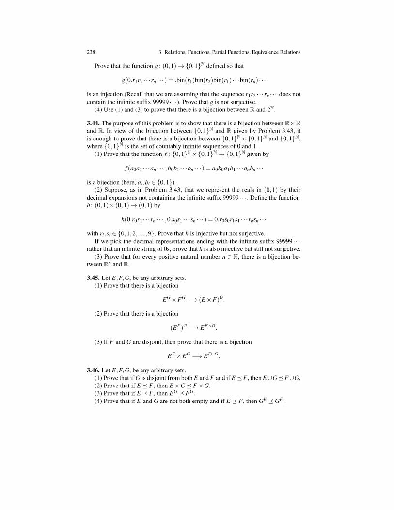
238 3 Relations, Functions, Partial Functions, Equivalence Relations
Prove that the function g : (0,1)→0,1N defined so that
g(0.r1r2 · · ·rn · · ·) = .bin(r1)bin(r2)bin(r1) · · ·bin(rn) · · ·
is an injection (Recall that we are assuming that the sequence r1r2 · · ·rn · · · does notcontain the infinite suffix 99999 · · · ). Prove that g is not surjective.
(4) Use (1) and (3) to prove that there is a bijection between R and 2N.
3.44. The purpose of this problem is to show that there is a bijection between R×Rand R. In view of the bijection between 0,1N and R given by Problem 3.43, itis enough to prove that there is a bijection between 0,1N×0,1N and 0,1N,where 0,1N is the set of countably infinite sequences of 0 and 1.
(1) Prove that the function f : 0,1N×0,1N→0,1N given by
f (a0a1 · · ·an · · · ,b0b1 · · ·bn · · ·) = a0b0a1b1 · · ·anbn · · ·
is a bijection (here, ai,bi ∈ 0,1).(2) Suppose, as in Problem 3.43, that we represent the reals in (0,1) by their
decimal expansions not containing the infinite suffix 99999 · · · . Define the functionh : (0,1)× (0,1)→ (0,1) by
h(0.r0r1 · · ·rn · · · ,0.s0s1 · · ·sn · · ·) = 0.r0s0r1s1 · · ·rnsn · · ·
with ri,si ∈ 0,1,2, . . . ,9. Prove that h is injective but not surjective.If we pick the decimal representations ending with the infinite suffix 99999 · · ·
rather that an infinite string of 0s, prove that h is also injective but still not surjective.(3) Prove that for every positive natural number n ∈ N, there is a bijection be-
tween Rn and R.
3.45. Let E,F,G, be any arbitrary sets.(1) Prove that there is a bijection
EG×FG −→ (E×F)G.
(2) Prove that there is a bijection
(EF)G −→ EF×G.
(3) If F and G are disjoint, then prove that there is a bijection
EF ×EG −→ EF∪G.
3.46. Let E,F,G, be any arbitrary sets.(1) Prove that if G is disjoint from both E and F and if E F , then E∪GF∪G.(2) Prove that if E F , then E×G F×G.(3) Prove that if E F , then EG FG.(4) Prove that if E and G are not both empty and if E F , then GE GF .
References 239
References
1. John H. Conway and K. Guy, Richard. The Book of Numbers. Copernicus. New York:Springer-Verlag, first edition, 1996.
2. Herbert B. Enderton. Elements of Set Theory. New York: Academic Press, first edition, 1977.3. Eric J. Stollnitz, Tony D. DeRose, and David H. Salesin. Wavelets for Computer Graphics
Theory and Applications. Morgan Kaufmann, first edition, 1996.4. Gilbert Strang and Nguyen Truong. Wavelets and Filter Banks. Wellesley-Cambridge Press,
second edition, 1997.5. Patrick Suppes. Axiomatic Set Theory. New York: Dover, first edition, 1972.

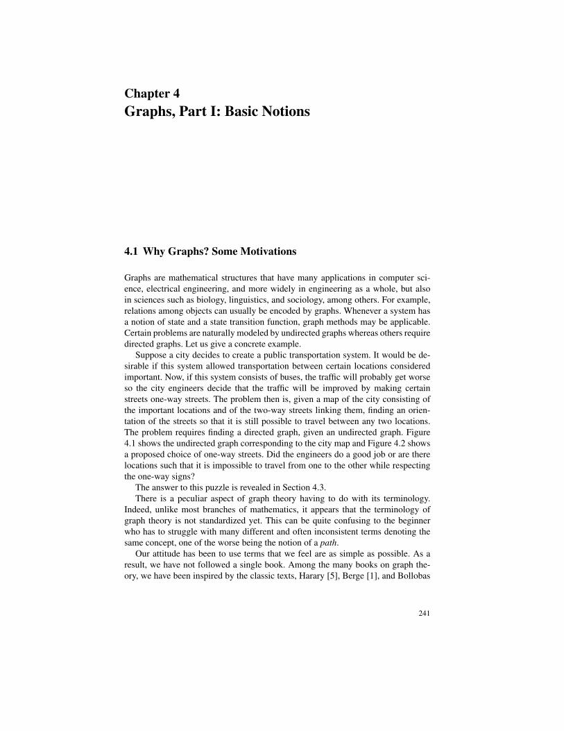
Chapter 4Graphs, Part I: Basic Notions
4.1 Why Graphs? Some Motivations
Graphs are mathematical structures that have many applications in computer sci-ence, electrical engineering, and more widely in engineering as a whole, but alsoin sciences such as biology, linguistics, and sociology, among others. For example,relations among objects can usually be encoded by graphs. Whenever a system hasa notion of state and a state transition function, graph methods may be applicable.Certain problems are naturally modeled by undirected graphs whereas others requiredirected graphs. Let us give a concrete example.
Suppose a city decides to create a public transportation system. It would be de-sirable if this system allowed transportation between certain locations consideredimportant. Now, if this system consists of buses, the traffic will probably get worseso the city engineers decide that the traffic will be improved by making certainstreets one-way streets. The problem then is, given a map of the city consisting ofthe important locations and of the two-way streets linking them, finding an orien-tation of the streets so that it is still possible to travel between any two locations.The problem requires finding a directed graph, given an undirected graph. Figure4.1 shows the undirected graph corresponding to the city map and Figure 4.2 showsa proposed choice of one-way streets. Did the engineers do a good job or are therelocations such that it is impossible to travel from one to the other while respectingthe one-way signs?
The answer to this puzzle is revealed in Section 4.3.There is a peculiar aspect of graph theory having to do with its terminology.
Indeed, unlike most branches of mathematics, it appears that the terminology ofgraph theory is not standardized yet. This can be quite confusing to the beginnerwho has to struggle with many different and often inconsistent terms denoting thesame concept, one of the worse being the notion of a path.
Our attitude has been to use terms that we feel are as simple as possible. As aresult, we have not followed a single book. Among the many books on graph the-ory, we have been inspired by the classic texts, Harary [5], Berge [1], and Bollobas
241
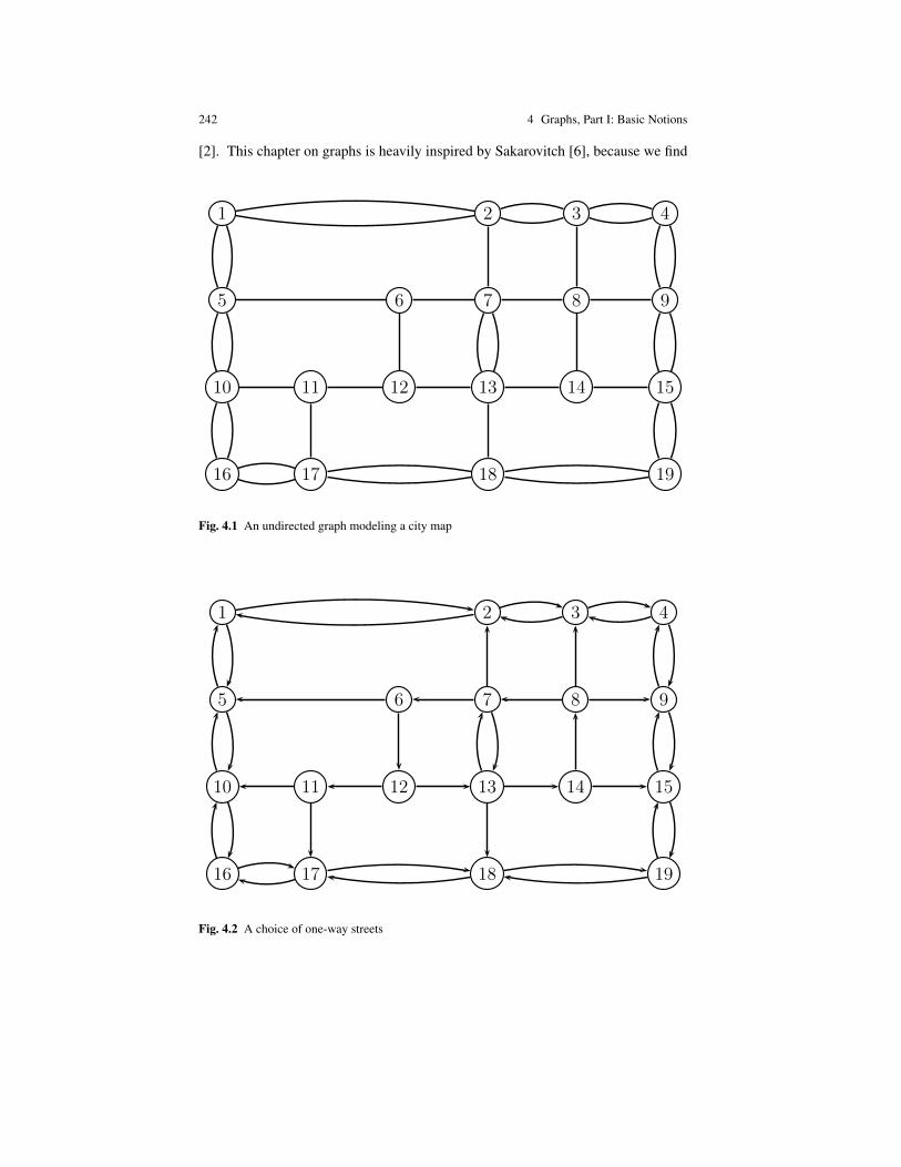
242 4 Graphs, Part I: Basic Notions
[2]. This chapter on graphs is heavily inspired by Sakarovitch [6], because we find
1
16 17 18 19
10 11 12 13 14 15
5 6 7 8 9
1 2 3 4
Fig. 4.1 An undirected graph modeling a city map
1
16 17 18 19
10 11 12 13 14 15
5 6 7 8 9
1 2 3 4
Fig. 4.2 A choice of one-way streets

4.2 Directed Graphs 243
Sakarovitch’s book extremely clear and because it has more emphasis on applica-tions than the previous two. Another more recent (and more advanced) text whichis also excellent is Diestel [4].
Fig. 4.3 Claude Berge, 1926–2002 (left) and Frank Harary, 1921–2005 (right)
Many books begin by discussing undirected graphs and introduce directed graphsonly later on. We disagree with this approach. Indeed, we feel that the notion of adirected graph is more fundamental than the notion of an undirected graph. For onething, a unique undirected graph is obtained from a directed graph by forgetting thedirection of the arcs, whereas there are many ways of orienting an undirected graph.Also, in general, we believe that most definitions about directed graphs are cleanerthan the corresponding ones for undirected graphs (for instance, we claim that thedefinition of a directed graph is simpler than the definition of an undirected graph,and similarly for paths). Thus, we begin with directed graphs.
4.2 Directed Graphs
Informally, a directed graph consists of a set of nodes together with a set of orientedarcs (also called edges) between these nodes. Every arc has a single source (or initialpoint) and a single target (or endpoint), both of which are nodes. There are variousways of formalizing what a directed graph is and some decisions must be made.Two issues must be confronted:
1. Do we allow “loops,” that is, arcs whose source and target are identical?2. Do we allow “parallel arcs,” that is, distinct arcs having the same source and
target?
For example, in the graph displayed on Figure 4.4, the edge e5 from v1 to itselfis a loop, and the two edges e1 and e2 from v1 to v2 are parallel edges.
Every binary relation on a set can be represented as a directed graph with loops,thus our definition allows loops. The directed graphs used in automata theory mustaccomodate parallel arcs (usually labeled with different symbols), therefore our def-inition also allows parallel arcs. Thus we choose a more inclusive definition in order

244 4 Graphs, Part I: Basic Notions
v3
v1 v2
e1
e2
e4e3
e5
Fig. 4.4 A directed graph
to accomodate as many applications as possible, even though some authors placerestrictions on the definition of a graph, for example, forbidding loops and parallelarcs (we call graphs without parallel arcs, simple graphs).
Before giving a formal definition, let us say that graphs are usually depicted bydrawings (graphs!) where the nodes are represented by circles containing the nodename and oriented line segments labeled with their arc name (see Figures 4.4 and4.5).
It should be emphasized that a directed graph (or any type of graph) is determinedby its edges; the vertices are only needed to anchor each edge by specifying itssource and its target. This can be done by defining two functions s (for source) andt (for target) that assign a source s(e) and a target t(e) to every edge e. For example,for the graph in Figure 4.4, edge e1 has source s(e1) = v1 and target t(e1) = v2; edgee4 has source s(e4) = v2 and target t(e4) = v3, and edge e5 (a loop) has identicalsource and target s(e5) = t(e5) = v1.
Definition 4.1. A directed graph (or digraph) is a quadruple G = (V,E,s, t), whereV is a set of nodes or vertices, E is a set of arcs or edges, and s, t : E → V are twofunctions, s being called the source function and t the target function. Given an edgee ∈ E, we also call s(e) the origin or source of e, and t(e) the endpoint or target ofe.
If the context makes it clear that we are dealing only with directed graphs,we usually say simply “graph” instead of “directed graph.” A directed graph,G = (V,E,s, t), is finite iff both V and E are finite. In this case, |V |, the numberof nodes of G, is called the order of G.
Example: Let G1 be the directed graph defined such thatE = e1,e2,e3,e4,e5,e6,e7,e8,e9,V = v1,v2,v3,v4,v5,v6, and

4.2 Directed Graphs 245
s(e1) = v1,s(e2) = v2,s(e3) = v3,s(e4) = v4,
s(e5) = v2,s(e6) = v5,s(e7) = v5,s(e8) = v5,s(e9) = v6
t(e1) = v2, t(e2) = v3, t(e3) = v4, t(e4) = v2,
t(e5) = v5, t(e6) = v5, t(e7) = v6, t(e8) = v6, t(e9) = v4.
The graph G1 is represented by the diagram shown in Figure 4.5.
1
v1 v2
v3
v4
v5 v6
e7
e8
e9
e1
e2
e3
e4
e5
e6
Fig. 4.5 A directed graph G1
It should be noted that there are many different ways of “drawing” a graph. Ob-viously, we would like as much as possible to avoid having too many intersectingarrows but this is not always possible if we insist on drawing a graph on a sheet ofpaper (on the plane).
Definition 4.2. Given a directed graph G, an edge e ∈ E, such that s(e) = t(e) iscalled a loop (or self-loop). Two edges e,e′ ∈ E are said to be parallel edges iffs(e) = s(e′) and t(e) = t(e′). A directed graph is simple iff it has no parallel edges.
Remarks:
1. The functions s, t need not be injective or surjective. Thus, we allow “isolatedvertices,” that is, vertices that are not the source or the target of any edge.
2. When G is simple, every edge e ∈ E, is uniquely determined by the ordered pairof vertices (u,v), such that u = s(e) and v = t(e). In this case, we may denotethe edge e by (uv) (some books also use the notation uv). Also, a graph without
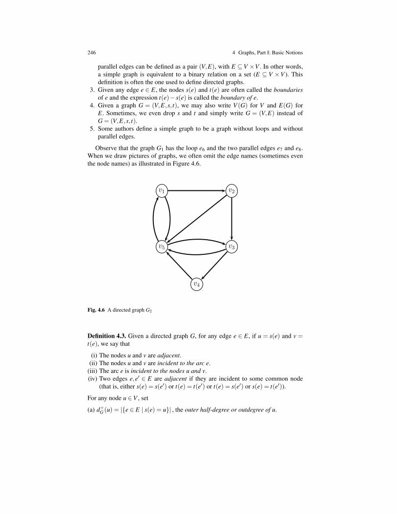
246 4 Graphs, Part I: Basic Notions
parallel edges can be defined as a pair (V,E), with E ⊆ V ×V . In other words,a simple graph is equivalent to a binary relation on a set (E ⊆ V ×V ). Thisdefinition is often the one used to define directed graphs.
3. Given any edge e ∈ E, the nodes s(e) and t(e) are often called the boundariesof e and the expression t(e)− s(e) is called the boundary of e.
4. Given a graph G = (V,E,s, t), we may also write V (G) for V and E(G) forE. Sometimes, we even drop s and t and simply write G = (V,E) instead ofG = (V,E,s, t).
5. Some authors define a simple graph to be a graph without loops and withoutparallel edges.
Observe that the graph G1 has the loop e6 and the two parallel edges e7 and e8.When we draw pictures of graphs, we often omit the edge names (sometimes eventhe node names) as illustrated in Figure 4.6.
1
v4
v5 v3
v1 v2
Fig. 4.6 A directed graph G2
Definition 4.3. Given a directed graph G, for any edge e ∈ E, if u = s(e) and v =t(e), we say that
(i) The nodes u and v are adjacent.(ii) The nodes u and v are incident to the arc e.
(iii) The arc e is incident to the nodes u and v.(iv) Two edges e,e′ ∈ E are adjacent if they are incident to some common node
(that is, either s(e) = s(e′) or t(e) = t(e′) or t(e) = s(e′) or s(e) = t(e′)).
For any node u ∈V , set
(a) d+G (u) = |e ∈ E | s(e) = u| , the outer half-degree or outdegree of u.

4.2 Directed Graphs 247
(b) d−G (u) = |e ∈ E | t(e) = u| , the inner half-degree or indegree of u.(c) dG(u) = d+
G (u)+d−G (u) , the degree of u.
A graph is regular iff every node has the same degree.
Note that d+G (respectively, d−G (u)) counts the number of arcs “coming out from
u,” that is, whose source is u (respectively, counts the number of arcs “coming intou,” i.e., whose target is u). For example, in the graph of Figure 4.6, d+
G2(v1) = 2,
d−G2(v1) = 1, d+
G2(v5) = 2, d−G2
(v5) = 4, d+G2(v3) = 2, d−G2
(v3) = 2. Neither G1 norG2 are regular graphs.
The first result of graph theory is the following simple but very useful proposi-tion.
Proposition 4.1. For any finite graph G = (V,E,s, t) we have
∑u∈V
d+G (u) = ∑
u∈Vd−G (u).
Proof . Every arc e ∈ E has a single source and a single target and each side of theabove equations simply counts the number of edges in the graph. ut
Corollary 4.1. For any finite graph G = (V,E,s, t) we have
∑u∈V
dG(u) = 2|E|;
that is, the sum of the degrees of all the nodes is equal to twice the number of edges.
Corollary 4.2. For any finite graph G = (V,E,s, t) there is an even number of nodeswith an odd degree.
The notion of homomorphism and isomorphism of graphs is fundamental.
Definition 4.4. Given two directed graphs G1 = (V1,E1,s1, t1) and G2 = (V2,E2,s2,t2), a homomorphism (or morphism) f : G1→G2 from G1 to G2 is a pair f =( f v, f e)with f v : V1 → V2 and f e : E1 → E2 preserving incidence; that is, for every edge,e ∈ E1, we have
s2( f e(e)) = f v(s1(e)) and t2( f e(e)) = f v(t1(e)).
These conditions can also be expressed by saying that the following two diagramscommute:
E1f e//
s1
E2
s2
V1 f v
// V2
E1f e//
t1
E2
t2
V1 f v// V2.

248 4 Graphs, Part I: Basic Notions
Given three graphs G1,G2,G3 and two homomorphisms f : G1→ G2, g : G2→G3, with f = ( f v, f e) and g = (gv,ge), it is easily checked that (gv f v,ge f e) isa homomorphism from G1 to G3. The homomorphism (gv f v,ge f e) is denotedg f . Also, for any graph G, the map idG = (idV , idE) is a homomorphism called theidentity homomorphism. Then, a homomorphism f : G1→G2 is an isomorphism iffthere is a homomorphism, g : G2→ G1, such that
g f = idG1 and f g = idG2 .
In this case, g is unique and it is called the inverse of f and denoted f−1. Iff = ( f v, f e) is an isomorphism, we see immediately that f v and f e are bijections.Checking whether two finite graphs are isomorphic is not as easy as it looks. Infact, no general efficient algorithm for checking graph isomorphism is known at thistime and determining the exact complexity of this problem is a major open questionin computer science. For example, the graphs G3 and G4 shown in Figure 4.7 areisomorphic. The bijection f v is given by f v(vi) = wi, for i = 1, . . . ,6 and the readerwill easily figure out the bijection on arcs. As we can see, isomorphic graphs canlook quite different.
1
v4 v5 v6
v1 v2 v3
G3 :
w4
w5
w6
w1
w2
w3
G4 :
Fig. 4.7 Two isomorphic graphs, G3 and G4
4.3 Paths in Digraphs; Strongly Connected Components
Many problems about graphs can be formulated as path existence problems. Given adirected graph G, intuitively, a path from a node u to a node v is a way to travel from
4.3 Path in Digraphs; Strongly Connected Components 249
u in v by following edges of the graph that “link up correctly.” Unfortunately, if welook up the definition of a path in two different graph theory books, we are almostguaranteed to find different and usually clashing definitions. This has to do with thefact that for some authors, a path may not use the same edge more than once and forothers, a path may not pass through the same node more than once. Moreover, whenparallel edges are present (i.e., when a graph is not simple), a sequence of nodesdoes not define a path unambiguously.
The terminology that we have chosen may not be standard, but it is used by anumber of authors (some very distinguished, e.g., Fields medalists) and we believethat it is less taxing on one’s memory (however, this point is probably the mostdebatable).
Definition 4.5. Given any digraph G=(V,E,s, t), and any two nodes u,v∈V , a pathfrom u to v is a triple, π = (u,e1 · · ·en,v), where n≥ 1 and e1 · · ·en is a sequence ofedges, ei ∈ E (i.e., a nonempty string in E∗), such that
s(e1) = u; t(en) = v; t(ei) = s(ei+1), 1≤ i≤ n−1.
We call n the length of the path π and we write |π| = n. When n = 0, we have thenull path (u,ε,u), from u to u (recall, ε denotes the empty string); the null path haslength 0. If u = v, then π is called a closed path, else an open path. The path π =(u,e1 · · ·en,v) determines the sequence of nodes, nodes(π) = 〈u0, . . . ,un〉, whereu0 = u, un = v and ui = t(ei), for 1≤ i≤ n. We also set nodes((u,ε,u)) = 〈u,u〉.
An important issue is whether a path contains no repeated edges or no repeatedvertices. The following definition spells out the terminology.
Definition 4.6. Given any digraph G = (V,E,s, t), and any two nodes u,v ∈ V , apath π = (u,e1 · · ·en,v), is edge-simple, for short, e-simple iff ei 6= e j for all i 6=j (i.e., no edge in the path is used twice). A path π from u to v is simple iff novertex in nodes(π) occurs twice, except possibly for u if π is closed. Equivalently,if nodes(π) = 〈u0, . . . ,un〉, then π is simple iff either
1. ui 6= u j for all i, j with i 6= j and 0 ≤ i, j ≤ n, or π is closed (i.e., u0 = un), inwhich case
2. ui 6= u0 (= un) for all i with 1≤ i≤ n−1, and ui 6= u j for all i, j with i 6= j and1≤ i, j ≤ n−1.
The null path (u,ε,u), is considered e-simple and simple.
Remarks:
1. Other authors (such as Harary [5]) use the term walk for what we call a path. Theterm trail is also used for what we call an e-simple path and the term path forwhat we call a simple path. We decided to adopt the term “simple path” becauseit is prevalent in the computer science literature. However, note that Berge [1]and Sakarovitch [6] use the locution elementary path instead of simple path.
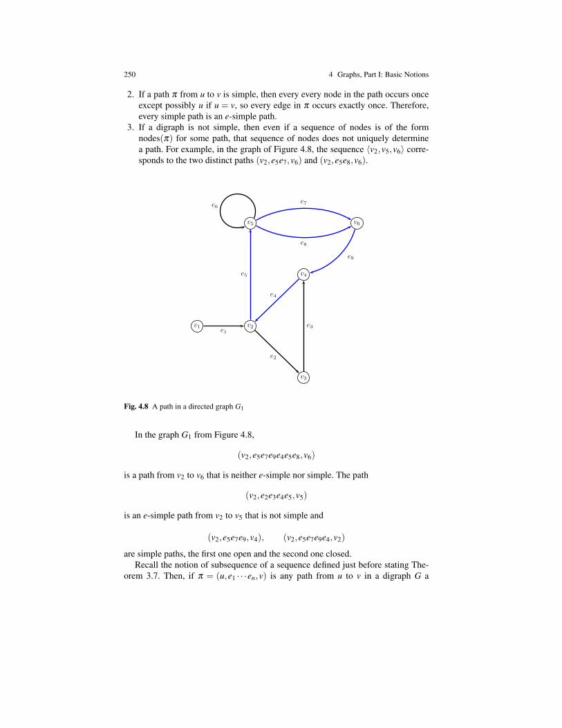
250 4 Graphs, Part I: Basic Notions
2. If a path π from u to v is simple, then every every node in the path occurs onceexcept possibly u if u = v, so every edge in π occurs exactly once. Therefore,every simple path is an e-simple path.
3. If a digraph is not simple, then even if a sequence of nodes is of the formnodes(π) for some path, that sequence of nodes does not uniquely determinea path. For example, in the graph of Figure 4.8, the sequence 〈v2,v5,v6〉 corre-sponds to the two distinct paths (v2,e5e7,v6) and (v2,e5e8,v6).
1
v1 v2
v3
v4
v5 v6
e7
e8
e9
e1
e2
e3
e4
e5
e6
Fig. 4.8 A path in a directed graph G1
In the graph G1 from Figure 4.8,
(v2,e5e7e9e4e5e8,v6)
is a path from v2 to v6 that is neither e-simple nor simple. The path
(v2,e2e3e4e5,v5)
is an e-simple path from v2 to v5 that is not simple and
(v2,e5e7e9,v4), (v2,e5e7e9e4,v2)
are simple paths, the first one open and the second one closed.Recall the notion of subsequence of a sequence defined just before stating The-
orem 3.7. Then, if π = (u,e1 · · ·en,v) is any path from u to v in a digraph G a

4.3 Path in Digraphs; Strongly Connected Components 251
1
v1 v2
v3
v4
v5 v6
e7
e8
e9
e1
e2
e3
e4
e5
e6
Fig. 4.9 An e-simple path in a directed graph G1
1
v1 v2
v3
v4
v5 v6
e7
e8
e9
e1
e2
e3
e4
e5
e6
Fig. 4.10 Simple paths in a directed graph G1
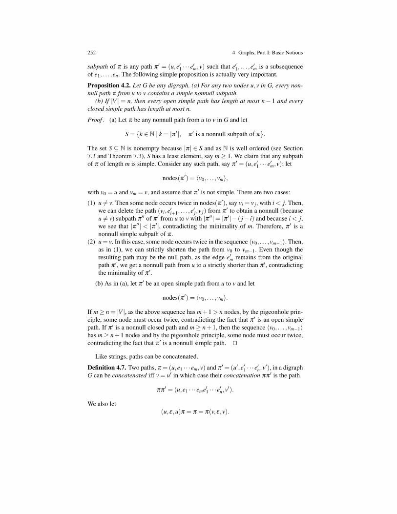
252 4 Graphs, Part I: Basic Notions
subpath of π is any path π ′ = (u,e′1 · · ·e′m,v) such that e′1, . . . ,e′m is a subsequence
of e1, . . . ,en. The following simple proposition is actually very important.
Proposition 4.2. Let G be any digraph. (a) For any two nodes u,v in G, every non-null path π from u to v contains a simple nonnull subpath.
(b) If |V | = n, then every open simple path has length at most n− 1 and everyclosed simple path has length at most n.
Proof . (a) Let π be any nonnull path from u to v in G and let
S = k ∈ N | k = |π ′|, π ′ is a nonnull subpath of π.
The set S ⊆ N is nonempty because |π| ∈ S and as N is well ordered (see Section7.3 and Theorem 7.3), S has a least element, say m≥ 1. We claim that any subpathof π of length m is simple. Consider any such path, say π ′ = (u,e′1 · · ·e′m,v); let
nodes(π ′) = 〈v0, . . . ,vm〉,
with v0 = u and vm = v, and assume that π ′ is not simple. There are two cases:
(1) u 6= v. Then some node occurs twice in nodes(π ′), say vi = v j, with i < j. Then,we can delete the path (vi,e′i+1, . . . ,e
′j,v j) from π ′ to obtain a nonnull (because
u 6= v) subpath π ′′ of π ′ from u to v with |π ′′|= |π ′|− ( j− i) and because i < j,we see that |π ′′| < |π ′|, contradicting the minimality of m. Therefore, π ′ is anonnull simple subpath of π .
(2) u= v. In this case, some node occurs twice in the sequence 〈v0, . . . ,vm−1〉. Then,as in (1), we can strictly shorten the path from v0 to vm−1. Even though theresulting path may be the null path, as the edge e′m remains from the originalpath π ′, we get a nonnull path from u to u strictly shorter than π ′, contradictingthe minimality of π ′.
(b) As in (a), let π ′ be an open simple path from u to v and let
nodes(π ′) = 〈v0, . . . ,vm〉.
If m≥ n = |V |, as the above sequence has m+1 > n nodes, by the pigeonhole prin-ciple, some node must occur twice, contradicting the fact that π ′ is an open simplepath. If π ′ is a nonnull closed path and m≥ n+1, then the sequence 〈v0, . . . ,vm−1〉has m≥ n+1 nodes and by the pigeonhole principle, some node must occur twice,contradicting the fact that π ′ is a nonnull simple path. ut
Like strings, paths can be concatenated.
Definition 4.7. Two paths, π = (u,e1 · · ·em,v) and π ′ = (u′,e′1 · · ·e′n,v′), in a digraphG can be concatenated iff v = u′ in which case their concatenation ππ ′ is the path
ππ′ = (u,e1 · · ·eme′1 · · ·e′n,v′).
We also let(u,ε,u)π = π = π(v,ε,v).
4.3 Path in Digraphs; Strongly Connected Components 253
Concatenation of paths is obviously associative and observe that |ππ ′| = |π|+|π ′|.
Definition 4.8. Let G = (V,E,s, t) be a digraph. We define the binary relation CG onV as follows. For all u,v ∈V ,
uCGv iff there is a path from u to v and there is a path from v to u.
When uCGv, we say that u and v are strongly connected.
The relation CG is an equivalence relation. The notion of an equivalence relationwas discussed in Chapter 3 (Section 3.9) but because it is a very important concept,we review its main properties.
Repeating Definition 3.11, a binary relation R on a set X is an equivalence rela-tion iff it is reflexive, transitive, and symmetric; that is:
(1) (Reflexivity): aRa, for all a ∈ X(2) (transitivity): If aRb and bRc, then aRc, for all a,b,c ∈ X(3) (Symmetry): If aRb, then bRa, for all a,b ∈ X
The main property of equivalence relations is that they partition the set X intononempty, pairwise disjoint subsets called equivalence classes: For any x ∈ X , theset
[x]R = y ∈ X | xRyis the equivalence class of x. Each equivalence class [x]R is also denoted xR and thesubscript R is often omitted when no confusion arises.
For the reader’s convenience, we repeat Proposition 3.5.
Let R be an equivalence relation on a set X. For any two elements x,y ∈ X, we have
xRy iff [x] = [y].
Moreover, the equivalence classes of R satisfy the following properties.
(1) [x] 6= /0, for all x ∈ X.(2) If [x] 6= [y] then [x]∩ [y] = /0.(3) X =
⋃x∈X [x].
The relation CG is reflexive because we have the null path from u to u, symmetricby definition, and transitive because paths can be concatenated. The equivalenceclasses of the relation CG are called the strongly connected components of G (SCCs).A graph is strongly connected iff it has a single strongly connected component.
For example, we see that the graph G1 of Figure 4.11 has two strongly connectedcomponents
v1, v2,v3,v4,v5,v6,inasmuch as there is a closed path
(v4,e4e2e3e4e5e7e9,v4).

254 4 Graphs, Part I: Basic Notions
1
v1 v2
v3
v4
v5 v6
e7
e8
e9
e1
e2
e3
e4
e5
e6
Fig. 4.11 A directed graph G1 with two SCCs
The graph G2 of Figure 4.6 is strongly connected.Let us give a simple algorithm for computing the strongly connected components
of a graph because this is often the key to solving many problems. The algorithmworks as follows. Given some vertex u ∈ V , the algorithm computes the two setsX+(u) and X−(u), where
X+(u) = v ∈V | there exists a path from u to vX−(u) = v ∈V | there exists a path from v to u.
Then, it is clear that the connected component C(u) of u, is given byC(u) = X+(u)∩X−(u).
For simplicity, we assume that X+(u),X−(u) and C(u) are represented by lineararrays. In order to make sure that the algorithm makes progress, we used a simplemarking scheme. We use the variable total to count how many nodes are in X+(u)(or in X−(u)) and the variable marked to keep track of how many nodes in X+(u)(or in X−(u)) have been processed so far. Whenever the algorithm considers someunprocessed node, the first thing it does is to increment marked by 1. Here is thealgorithm in high-level form.
function strcomp(G: graph; u: node): setbegin
4.3 Path in Digraphs; Strongly Connected Components 255
X+(u)[1] := u; X−(u)[1] := u; total := 1; marked := 0;while marked < total do
marked := marked+1; v := X+(u)[marked];for each e ∈ E
if (s(e) = v) & (t(e) /∈ X+(u)) thentotal := total+1; X+(u)[total] := t(e) endif
endforendwhile;total := 1; marked := 0;while marked < total do
marked := marked+1; v := X−(u)[marked];for each e ∈ E
if (t(e) = v) & (s(e) /∈ X−(u)) thentotal := total+1; X−(u)[total] := s(e) endif
endforendwhile;C(u) = X+(u)∩X−(u); strcomp :=C(u)
end
If we want to obtain all the strongly connected components (SCCs) of a finitegraph G, we proceed as follows. Set V1 = V , pick any node v1 in V1, and use theabove algorithm to compute the strongly connected component C1 of v1. If V1 =C1,stop. Otherwise, let V2 = V1−C1. Again, pick any node v2 in V2 and determine thestrongly connected component C2 of v2. If V2 =C2, stop. Otherwise, let V3 =V2−C2,pick v3 in V3, and continue in the same manner as before. Ultimately, this processwill stop and produce all the strongly connected components C1, . . . ,Ck of G.
It should be noted that the function strcomp and the simple algorithm that wejust described are “naive” algorithms that are not particularly efficient. Their mainadvantage is their simplicity. There are more efficient algorithms, in particular, thereis a beautiful algorithm for computing the SCCs due to Robert Tarjan.
Going back to our city traffic problem from Section 4.1, if we compute thestrongly connected components for the proposed solution shown in Figure 4.2, wefind three SCCs
A = 6,7,8,12,13,14, B = 11, C = 1,2,3,4,5,9,10,15,16,17,18,19.
shown in Figure 4.12.Therefore, the city engineers did not do a good job. We show after proving Propo-
sition 4.4 how to “fix” this faulty solution.Note that the problem is that all the edges between the strongly connected com-
ponents A and C go in the wrong direction.Closed e-simple paths also play an important role.
Definition 4.9. Let G = (V,E,s, t) be a digraph. A circuit is a closed e-simple path(i.e., no edge occurs twice) without a distinguished starting vertex, and a simplecircuit is a simple closed path (without a distinguished starting vertex). Two circuits

256 4 Graphs, Part I: Basic Notions
1
16 17 18 19
10 11 12 13 14 15
5 6 7 8 9
1 2 3 4
Fig. 4.12 The strongly connected components of the graph in Figure 4.2
or simple circuits obtained form each other by a cyclic permutation of their edgesequences are considered to be equal. Every null path (u,ε,u) is a simple circuit.
For example, in the graph G1 shown in Figure 4.10, the closed path
(v2,e5e7e9e4,v2)
is a circuit, in fact a simple circuit, and all closed paths
(v5,e7e9e4e5,v5), (v6,e9e4e5e7,v5), (v4,e4e5e7e9,v4),
obtained from it by cyclic permutation of the edges in the path are considered to bethe same circuit.
Remark: A closed path is sometimes called a pseudo-circuit. In a pseudo-circuit,some edge may occur more than once.
The significance of simple circuits is revealed by the next proposition.
Proposition 4.3. Let G be any digraph. (a) Every circuit π in G is the concatenationof pairwise edge-disjoint simple circuits.
(b) A circuit is simple iff it is a minimal circuit, that is, iff it does not contain anyproper circuit.
Proof . We proceed by induction on the length of π . The proposition is trivially trueif π is the null path. Next, let π = (u,e1 · · ·em,u) be any nonnull circuit and let
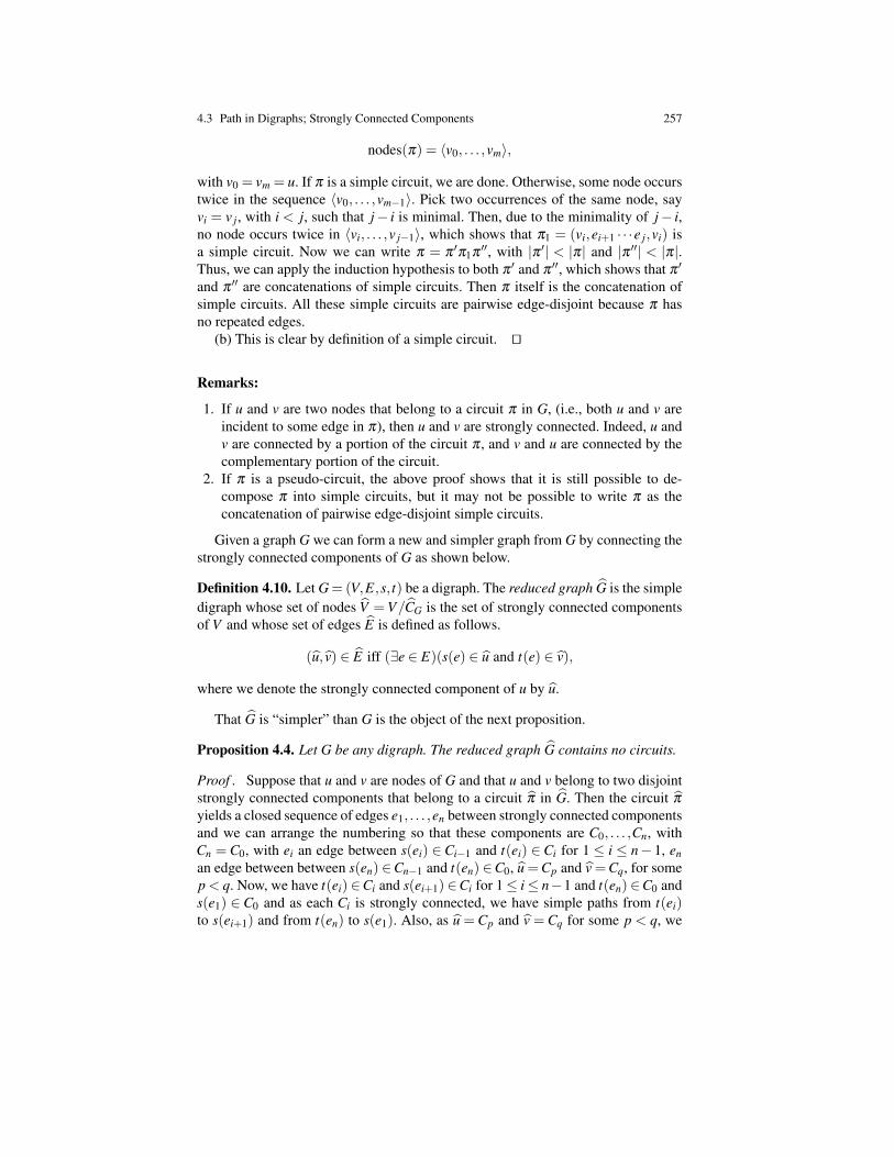
4.3 Path in Digraphs; Strongly Connected Components 257
nodes(π) = 〈v0, . . . ,vm〉,
with v0 = vm = u. If π is a simple circuit, we are done. Otherwise, some node occurstwice in the sequence 〈v0, . . . ,vm−1〉. Pick two occurrences of the same node, sayvi = v j, with i < j, such that j− i is minimal. Then, due to the minimality of j− i,no node occurs twice in 〈vi, . . . ,v j−1〉, which shows that π1 = (vi,ei+1 · · ·e j,vi) isa simple circuit. Now we can write π = π ′π1π ′′, with |π ′| < |π| and |π ′′| < |π|.Thus, we can apply the induction hypothesis to both π ′ and π ′′, which shows that π ′
and π ′′ are concatenations of simple circuits. Then π itself is the concatenation ofsimple circuits. All these simple circuits are pairwise edge-disjoint because π hasno repeated edges.
(b) This is clear by definition of a simple circuit. ut
Remarks:
1. If u and v are two nodes that belong to a circuit π in G, (i.e., both u and v areincident to some edge in π), then u and v are strongly connected. Indeed, u andv are connected by a portion of the circuit π , and v and u are connected by thecomplementary portion of the circuit.
2. If π is a pseudo-circuit, the above proof shows that it is still possible to de-compose π into simple circuits, but it may not be possible to write π as theconcatenation of pairwise edge-disjoint simple circuits.
Given a graph G we can form a new and simpler graph from G by connecting thestrongly connected components of G as shown below.
Definition 4.10. Let G= (V,E,s, t) be a digraph. The reduced graph G is the simpledigraph whose set of nodes V =V/CG is the set of strongly connected componentsof V and whose set of edges E is defined as follows.
(u, v) ∈ E iff (∃e ∈ E)(s(e) ∈ u and t(e) ∈ v),
where we denote the strongly connected component of u by u.
That G is “simpler” than G is the object of the next proposition.
Proposition 4.4. Let G be any digraph. The reduced graph G contains no circuits.
Proof . Suppose that u and v are nodes of G and that u and v belong to two disjointstrongly connected components that belong to a circuit π in G. Then the circuit π
yields a closed sequence of edges e1, . . . ,en between strongly connected componentsand we can arrange the numbering so that these components are C0, . . . ,Cn, withCn = C0, with ei an edge between s(ei) ∈Ci−1 and t(ei) ∈Ci for 1 ≤ i ≤ n− 1, enan edge between between s(en) ∈Cn−1 and t(en) ∈C0, u =Cp and v =Cq, for somep < q. Now, we have t(ei) ∈Ci and s(ei+1) ∈Ci for 1≤ i≤ n−1 and t(en) ∈C0 ands(e1) ∈ C0 and as each Ci is strongly connected, we have simple paths from t(ei)to s(ei+1) and from t(en) to s(e1). Also, as u = Cp and v = Cq for some p < q, we

258 4 Graphs, Part I: Basic Notions
have some simple paths from u to s(ep+1) and from t(eq) to v. By concatenatingthe appropriate paths, we get a circuit in G containing u and v, showing that u andv are strongly connected, contradicting that u and v belong to two disjoint stronglyconnected components. ut
Definition 4.11. A digraph without circuits is called a directed acyclic graph, forshort a DAGs.
Such graphs have many nice properties. In particular, it is easy to see that anyfinite DAG has nodes with no incoming edges. Then, it is easy to see that finiteDAGs are basically collections of trees with shared nodes.
The reduced graph (DAG) of the graph shown in Figure 4.12 is shown in Figure4.13, where its SCCs are labeled A, B, and C as shown below:
A = 6,7,8,12,13,14, B = 11, C = 1,2,3,4,5,9,10,15,16,17,18,19.
The locations in the component A are inaccessible. Observe that changing the di-
1
A
B C
Fig. 4.13 The reduced graph of the graph in Figure 4.12
rection of any street between the strongly connected components A and C yields asolution, that is, a strongly connected graph. So, the engineers were not too far offafter all.
A solution to our traffic problem obtained by changing the direction of the streetbetween 13 and 18 is shown in Figure 4.14. Before discussing undirected graphs,let us collect various definitions having to do with the notion of subgraph.
Definition 4.12. Given any two digraphs G = (V,E,s, t) and G′ = (V ′,E ′,s′, t ′), wesay that G′ is a subgraph of G iff V ′ ⊆V , E ′ ⊆ E, s′ is the restriction of s to E ′ andt ′ is the restriction of t to E ′. If G′ is a subgraph of G and V ′ =V , we say that G′ isa spanning subgraph of G. Given any subset V ′ of V , the induced subgraph G〈V ′〉of G is the graph (V ′,EV ′ ,s′, t ′) whose set of edges is
EV ′ = e ∈ E | s(e) ∈V ′; t(e) ∈V ′.
(Clearly, s′ and t ′ are the restrictions of s and t to EV ′ , respectively.) Given anysubset, E ′ ⊆ E, the graph G′ = (V,E ′,s′, t ′), where s′ and t ′ are the restrictions of sand t to E ′, respectively, is called the partial graph of G generated by E ′.
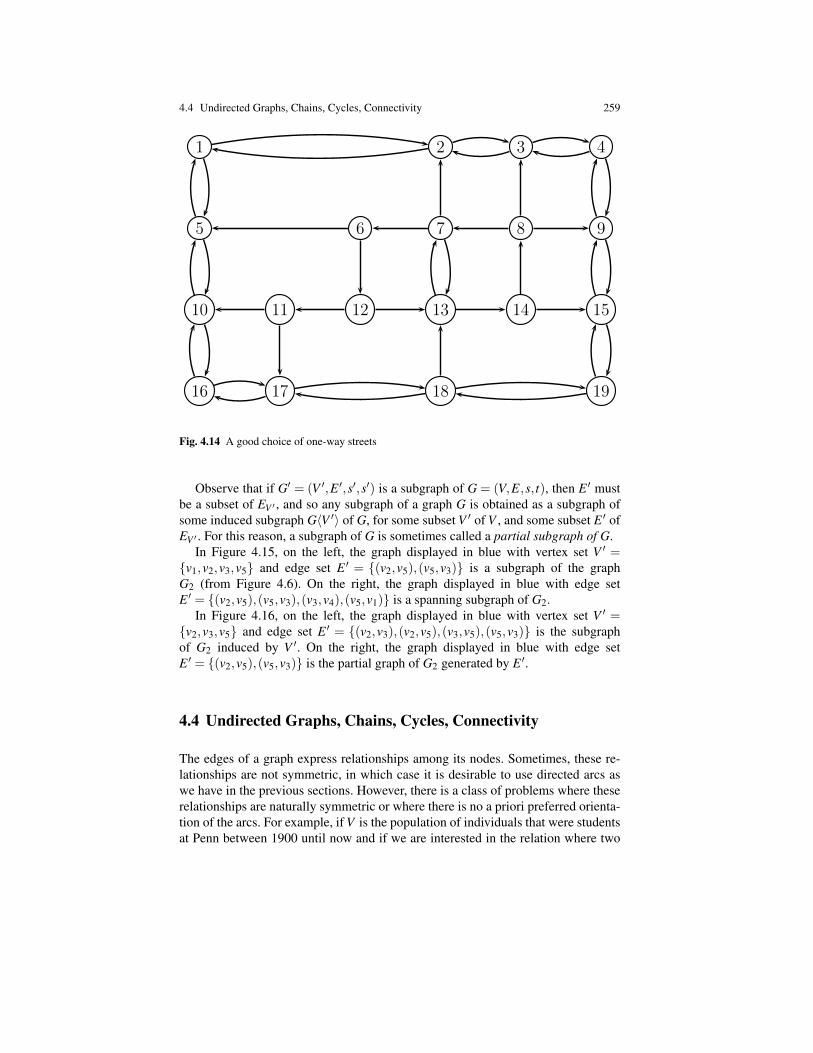
4.4 Undirected Graphs, Chains, Cycles, Connectivity 259
1
16 17 18 19
10 11 12 13 14 15
5 6 7 8 9
1 2 3 4
Fig. 4.14 A good choice of one-way streets
Observe that if G′ = (V ′,E ′,s′,s′) is a subgraph of G = (V,E,s, t), then E ′ mustbe a subset of EV ′ , and so any subgraph of a graph G is obtained as a subgraph ofsome induced subgraph G〈V ′〉 of G, for some subset V ′ of V , and some subset E ′ ofEV ′ . For this reason, a subgraph of G is sometimes called a partial subgraph of G.
In Figure 4.15, on the left, the graph displayed in blue with vertex set V ′ =v1,v2,v3,v5 and edge set E ′ = (v2,v5),(v5,v3) is a subgraph of the graphG2 (from Figure 4.6). On the right, the graph displayed in blue with edge setE ′ = (v2,v5),(v5,v3),(v3,v4),(v5,v1) is a spanning subgraph of G2.
In Figure 4.16, on the left, the graph displayed in blue with vertex set V ′ =v2,v3,v5 and edge set E ′ = (v2,v3),(v2,v5),(v3,v5),(v5,v3) is the subgraphof G2 induced by V ′. On the right, the graph displayed in blue with edge setE ′ = (v2,v5),(v5,v3) is the partial graph of G2 generated by E ′.
4.4 Undirected Graphs, Chains, Cycles, Connectivity
The edges of a graph express relationships among its nodes. Sometimes, these re-lationships are not symmetric, in which case it is desirable to use directed arcs aswe have in the previous sections. However, there is a class of problems where theserelationships are naturally symmetric or where there is no a priori preferred orienta-tion of the arcs. For example, if V is the population of individuals that were studentsat Penn between 1900 until now and if we are interested in the relation where two
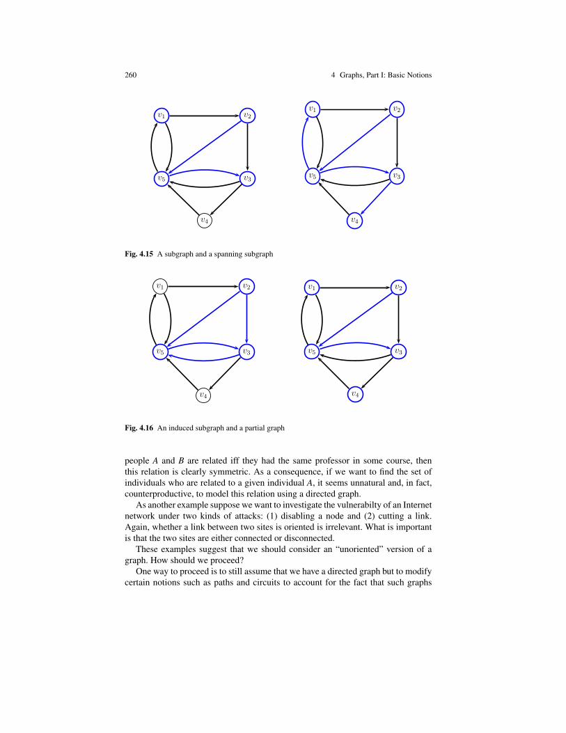
260 4 Graphs, Part I: Basic Notions
v4
v5 v3
v1 v2
v4
v5 v3
v1 v2
Fig. 4.15 A subgraph and a spanning subgraph
v4
v5 v3
v1 v2
v4
v5 v3
v1 v2
Fig. 4.16 An induced subgraph and a partial graph
people A and B are related iff they had the same professor in some course, thenthis relation is clearly symmetric. As a consequence, if we want to find the set ofindividuals who are related to a given individual A, it seems unnatural and, in fact,counterproductive, to model this relation using a directed graph.
As another example suppose we want to investigate the vulnerabilty of an Internetnetwork under two kinds of attacks: (1) disabling a node and (2) cutting a link.Again, whether a link between two sites is oriented is irrelevant. What is importantis that the two sites are either connected or disconnected.
These examples suggest that we should consider an “unoriented” version of agraph. How should we proceed?
One way to proceed is to still assume that we have a directed graph but to modifycertain notions such as paths and circuits to account for the fact that such graphs

4.4 Undirected Graphs, Chains, Cycles, Connectivity 261
are really “unoriented.” In particular, we should redefine paths to allow edges tobe traversed in the “wrong direction.” Such an approach is possible but slightlyawkward and ultimately it is really better to define undirected graphs. However,to show that this approach is feasible, let us give a new definition of a path thatcorresponds to the notion of path in an undirected graph.
Definition 4.13. Given any digraph G = (V,E,s, t) and any two nodes u,v ∈ V , achain (or walk) from u to v is a sequence π = (u0,e1,u1,e2,u2, . . . ,un−1,en,un),where n≥ 1; ui ∈V ; e j ∈ E and
u0 = u; un = v and s(ei), t(ei)= ui−1,ui, 1≤ i≤ n.
We call n the length of the chain π and we write |π| = n. When n = 0, we havethe null chain (u,ε,u), from u to u, a chain of length 0. If u = v, then π is calleda closed chain, else an open chain. The chain π determines the sequence of nodes:nodes(π) = 〈u0, . . . ,un〉, with nodes((u,ε,u)) = 〈u,u〉.
The following definition is the version of Definition 4.6 for chains that containno repeated edges or no repeated vertices.
Definition 4.14. Given any digraph G = (V,E,s, t) and any two nodes u,v ∈ V , achain π is edge-simple, for short, e-simple iff ei 6= e j for all i 6= j (i.e., no edge in thechain is used twice). A chain π from u to v is simple iff no vertex in nodes(π) occurstwice, except possibly for u if π is closed. The null chain (u,ε,u) is considered e-simple and simple.
The main difference between Definition 4.13 and Definition 4.5 is that Definition4.13 ignores the orientation: in a chain, an edge may be traversed backwards, fromits endpoint back to its source. This implies that the reverse of a chain
πR = (un,en,un−1, , . . . ,u2,e2,u1,e1,u0)
is a chain from v = un to u = u0. In general, this fails for paths. Note, as before, thatif G is a simple graph, then a chain is more simply defined by a sequence of nodes
(u0,u1, . . . ,un).
For example, in the graph G5 shown in Figure 4.17, we have the chains
(v1,a,v2,d,v4, f ,v5,e,v2,d,v4,g,v3), (v1,a,v2,d,v4, f ,v5,e,v2,c,v3)
and(v1,a,v2,d,v4,g,v3)
from v1 to v3.Note that none of these chains are paths. The graph G′5 is obtained from the graph
G5 by reversing the direction of the edges d, f , e, and g, so that the above chains areactually paths in G′5. The second chain is e-simple and the third is simple.

262 4 Graphs, Part I: Basic Notions
v4
v5
v1 v2
v3
a
g
b c d
e
f
G5 :
v4
v5
v1 v2
v3
a
g
b c d
e
f
G!5 :
Fig. 4.17 The graphs G5 and G′5
Chains are concatenated the same way as paths and the notion of subchain isanalogous to the notion of subpath. The undirected version of Proposition 4.2 alsoholds. The proof is obtained by changing the word “path” to “chain.”
Proposition 4.5. Let G be any digraph. (a) For any two nodes u,v in G, every non-null chain π from u to v contains a simple nonnull subchain.
(b) If |V | = n, then every open simple chain has length at most n− 1 and everyclosed simple chain has length at most n.
The undirected version of strong connectivity is the following:
Definition 4.15. Let G = (V,E,s, t) be a digraph. We define the binary relation CGon V as follows. For all u,v ∈V ,
uCGv iff there is a chain from u to v.
When uCGv, we say that u and v are connected.
Oberve that the relation CG is an equivalence relation. It is reflexive because wehave the null chain from u to u, symmetric because the reverse of a chain is also achain, and transitive because chains can be concatenated. The equivalence classesof the relation CG are called the connected components of G (CCs). A graph isconnected iff it has a single connected component.
Observe that strong connectivity implies connectivity but the converse is false.For example, the graph G1 of Figure 4.5 is connected but it is not strongly con-nected. The function strcomp and the method for computing the strongly connectedcomponents of a graph can easily be adapted to compute the connected componentsof a graph.
The undirected version of a circuit is the following.
Definition 4.16. Let G = (V,E,s, t) be a digraph. A cycle is a closed e-simple chain(i.e., no edge occurs twice) without a distinguished starting vertex, and a simple
4.4 Undirected Graphs, Chains, Cycles, Connectivity 263
cycle is a simple closed chain (without a distinguished starting vertex). Two cy-cles or simple cycle obtained form each other by a cyclic permutation of their edgesequences are considered to be equal. Every null chain (u,ε,u) is a simple cycle.
Remark: A closed chain is sometimes called a pseudo-cycle. The undirected ver-sion of Proposition 4.3 also holds. Again, the proof consists in changing the word“circuit” to “cycle”.
Proposition 4.6. Let G be any digraph. (a) Every cycle π in G is the concatenationof pairwise edge-disjoint simple cycles.
(b) A cycle is simple iff it is a minimal cycle, that is, iff it does not contain anyproper cycle.
The reader should now be convinced that it is actually possible to use the notionof a directed graph to model a large class of problems where the notion of orientationis irrelevant. However, this is somewhat unnatural and often inconvenient, so it isdesirable to introduce the notion of an undirected graph as a “first-class” object.How should we do that?
We could redefine the set of edges of an undirected graph to be of the formE+∪E−, where E+ = E is the original set of edges of a digraph and with
E− = e− | e+ ∈ E+, s(e−) = t(e+), t(e−) = s(e+),
each edge e− being the “anti-edge” (opposite edge) of e+. Such an approach isworkable but experience shows that it not very satisfactory.
The solution adopted by most people is to relax the condition that every edgee ∈ E be assigned an ordered pair 〈u,v〉 of nodes (with u = s(e) and v = t(e)) tothe condition that every edge e ∈ E be assigned a set u,v of nodes (with u = vallowed). To this effect, let [V ]2 denote the subset of the power set consisting of alltwo-element subsets of V (the notation
(V2
)is sometimes used instead of [V ]2):
[V ]2 = u,v ∈ 2V | u 6= v.
Definition 4.17. A graph is a triple G = (V,E,st) where V is a set of nodes orvertices, E is a set of arcs or edges, and st : E →V ∪ [V ]2 is a function that assignsa set of endpoints (or endnodes) to every edge.
When we want to stress that we are dealing with an undirected graph as opposedto a digraph, we use the locution undirected graph. When we draw an undirectedgraph we suppress the tip on the extremity of an arc. For example, the undirectedgraph G6 corresponding to the directed graph G5, is shown in Figure 4.18.
Definition 4.18. Given a graph G, an edge e ∈ E such that st(e) ∈V is called a loop(or self-loop). Two edges e,e′ ∈ E are said to be parallel edges iff st(e) = st(e′). Agraph is simple iff it has no loops and no parallel edges.
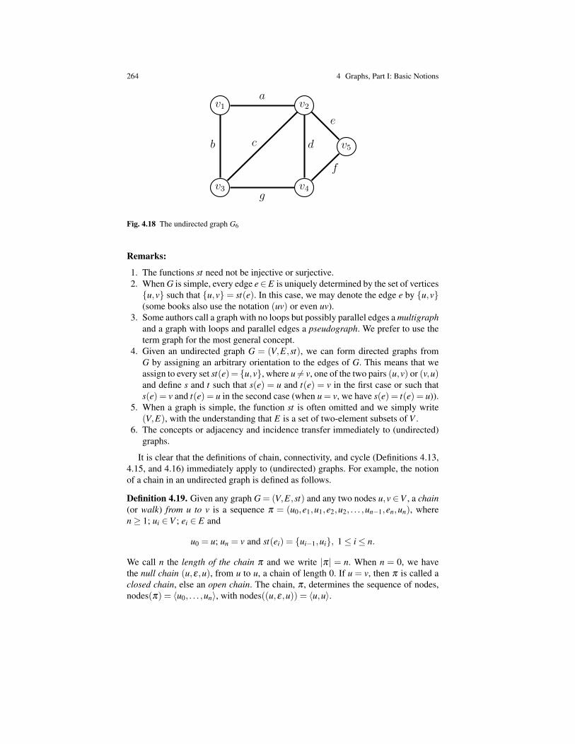
264 4 Graphs, Part I: Basic Notions
1
v4
v5
v1 v2
v3
a
g
b c d
e
f
Fig. 4.18 The undirected graph G6
Remarks:
1. The functions st need not be injective or surjective.2. When G is simple, every edge e∈E is uniquely determined by the set of verticesu,v such that u,v= st(e). In this case, we may denote the edge e by u,v(some books also use the notation (uv) or even uv).
3. Some authors call a graph with no loops but possibly parallel edges a multigraphand a graph with loops and parallel edges a pseudograph. We prefer to use theterm graph for the most general concept.
4. Given an undirected graph G = (V,E,st), we can form directed graphs fromG by assigning an arbitrary orientation to the edges of G. This means that weassign to every set st(e)= u,v, where u 6= v, one of the two pairs (u,v) or (v,u)and define s and t such that s(e) = u and t(e) = v in the first case or such thats(e) = v and t(e) = u in the second case (when u = v, we have s(e) = t(e) = u)).
5. When a graph is simple, the function st is often omitted and we simply write(V,E), with the understanding that E is a set of two-element subsets of V .
6. The concepts or adjacency and incidence transfer immediately to (undirected)graphs.
It is clear that the definitions of chain, connectivity, and cycle (Definitions 4.13,4.15, and 4.16) immediately apply to (undirected) graphs. For example, the notionof a chain in an undirected graph is defined as follows.
Definition 4.19. Given any graph G = (V,E,st) and any two nodes u,v ∈V , a chain(or walk) from u to v is a sequence π = (u0,e1,u1,e2,u2, . . . ,un−1,en,un), wheren≥ 1; ui ∈V ; ei ∈ E and
u0 = u; un = v and st(ei) = ui−1,ui, 1≤ i≤ n.
We call n the length of the chain π and we write |π| = n. When n = 0, we havethe null chain (u,ε,u), from u to u, a chain of length 0. If u = v, then π is called aclosed chain, else an open chain. The chain, π , determines the sequence of nodes,nodes(π) = 〈u0, . . . ,un〉, with nodes((u,ε,u)) = 〈u,u〉.

4.4 Undirected Graphs, Chains, Cycles, Connectivity 265
The next definition is the version of Definition 4.14 for undirected graphs.
Definition 4.20. Given any graph G = (V,E,st) and any two nodes u,v ∈V , a chainπ is edge-simple, for short, e-simple iff ei 6= e j for all i 6= j (i.e., no edge in the chainis used twice). A chain π from u to v is simple iff no vertex in nodes(π) occurs twice,except possibly for u if π is closed. The null chain (u,ε,u) is considered e-simpleand simple.
An e-simple chain is also called a trail (as in the case of directed graphs). Defi-nitions 4.15 and 4.16 are adapted to undirected graphs in a similar fashion.
However, only the notion of degree (or valency) of a node applies to undirectedgraphs where it is given by
dG(u) = |e ∈ E | u ∈ st(e)|.
We can check immediately that Corollary 4.1 and Corollary 4.2 apply to undirectedgraphs. For the reader’s convenience, we restate these results.
Corollary 4.3. For any finite undirected graph G = (V,E,st) we have
∑u∈V
dG(u) = 2|E|;
that is, the sum of the degrees of all the nodes is equal to twice the number of edges.
Corollary 4.4. For any finite undirected graph G = (V,E,st), there is an even num-ber of nodes with an odd degree.
Remark: When it is clear that we are dealing with undirected graphs, we some-times allow ourselves some abuse of language. For example, we occasionally usethe term path instead of chain.
An important class of graphs is the class of complete graphs. We define the com-plete graph Kn with n vertices (n ≥ 2) as the simple undirected graph whose edgesare all two-element subsets i, j, with i, j ∈ 1,2, . . . ,n and i 6= j.
Even though the structure of complete graphs is quite simple, there are some veryhard combinatorial problems involving them. For example, an amusing but verydifficult problem involving edge colorings is the determination of Ramsey numbers.
A version of Ramsey’s theorem says that: for every pair, (r,s), of positive naturalnumbers, there is a least positive natural number, R(r,s), such that for every coloringof the edges of the complete (undirected) graph on R(r,s) vertices using the colorsblue and red, either there is a complete subgraph with r vertices whose edges areall blue or there is a complete subgraph with s vertices whose edges are all red.
So, R(r,r) is the smallest number of vertices of a complete graph whose edgesare colored either blue or red that must contain a complete subgraph with r verticeswhose edges are all of the same color. It is called a Ramsey number. For details onRamsey’s theorems and Ramsey numbers, see Diestel [4], Chapter 9.
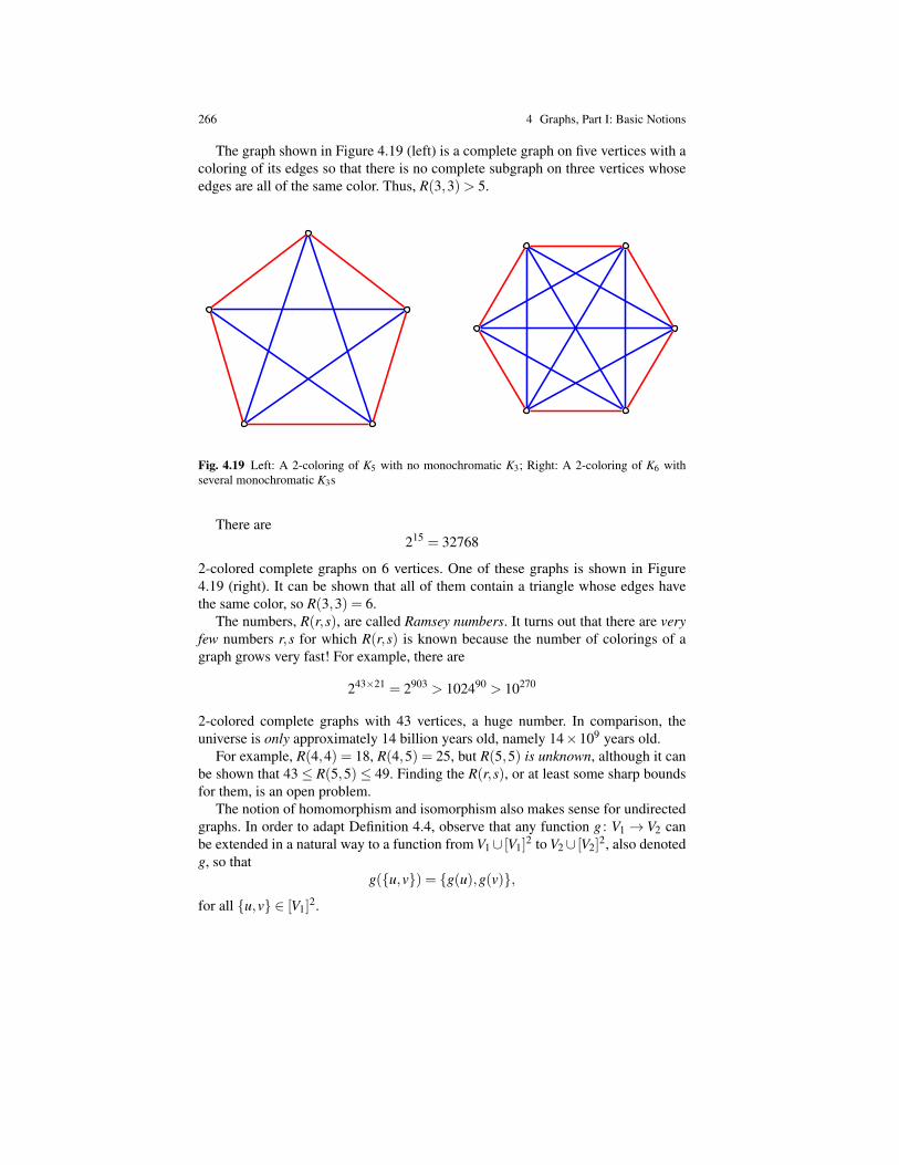
266 4 Graphs, Part I: Basic Notions
The graph shown in Figure 4.19 (left) is a complete graph on five vertices with acoloring of its edges so that there is no complete subgraph on three vertices whoseedges are all of the same color. Thus, R(3,3)> 5.
1
Fig. 4.19 Left: A 2-coloring of K5 with no monochromatic K3; Right: A 2-coloring of K6 withseveral monochromatic K3s
There are215 = 32768
2-colored complete graphs on 6 vertices. One of these graphs is shown in Figure4.19 (right). It can be shown that all of them contain a triangle whose edges havethe same color, so R(3,3) = 6.
The numbers, R(r,s), are called Ramsey numbers. It turns out that there are veryfew numbers r,s for which R(r,s) is known because the number of colorings of agraph grows very fast! For example, there are
243×21 = 2903 > 102490 > 10270
2-colored complete graphs with 43 vertices, a huge number. In comparison, theuniverse is only approximately 14 billion years old, namely 14×109 years old.
For example, R(4,4) = 18, R(4,5) = 25, but R(5,5) is unknown, although it canbe shown that 43≤ R(5,5)≤ 49. Finding the R(r,s), or at least some sharp boundsfor them, is an open problem.
The notion of homomorphism and isomorphism also makes sense for undirectedgraphs. In order to adapt Definition 4.4, observe that any function g : V1 → V2 canbe extended in a natural way to a function from V1∪ [V1]
2 to V2∪ [V2]2, also denoted
g, so thatg(u,v) = g(u),g(v),
for all u,v ∈ [V1]2.
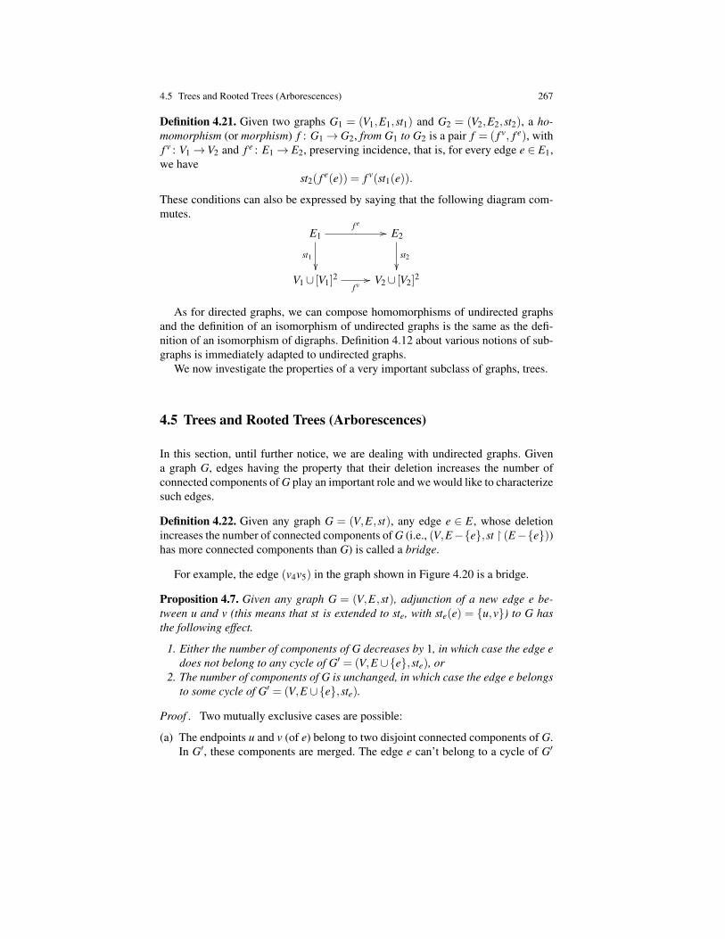
4.5 Trees and Rooted Trees (Arborescences) 267
Definition 4.21. Given two graphs G1 = (V1,E1,st1) and G2 = (V2,E2,st2), a ho-momorphism (or morphism) f : G1→G2, from G1 to G2 is a pair f = ( f v, f e), withf v : V1→V2 and f e : E1→ E2, preserving incidence, that is, for every edge e ∈ E1,we have
st2( f e(e)) = f v(st1(e)).
These conditions can also be expressed by saying that the following diagram com-mutes.
E1f e
//
st1
E2
st2
V1∪ [V1]2
f v// V2∪ [V2]
2
As for directed graphs, we can compose homomorphisms of undirected graphsand the definition of an isomorphism of undirected graphs is the same as the defi-nition of an isomorphism of digraphs. Definition 4.12 about various notions of sub-graphs is immediately adapted to undirected graphs.
We now investigate the properties of a very important subclass of graphs, trees.
4.5 Trees and Rooted Trees (Arborescences)
In this section, until further notice, we are dealing with undirected graphs. Givena graph G, edges having the property that their deletion increases the number ofconnected components of G play an important role and we would like to characterizesuch edges.
Definition 4.22. Given any graph G = (V,E,st), any edge e ∈ E, whose deletionincreases the number of connected components of G (i.e., (V,E−e,st (E−e))has more connected components than G) is called a bridge.
For example, the edge (v4v5) in the graph shown in Figure 4.20 is a bridge.
Proposition 4.7. Given any graph G = (V,E,st), adjunction of a new edge e be-tween u and v (this means that st is extended to ste, with ste(e) = u,v) to G hasthe following effect.
1. Either the number of components of G decreases by 1, in which case the edge edoes not belong to any cycle of G′ = (V,E ∪e,ste), or
2. The number of components of G is unchanged, in which case the edge e belongsto some cycle of G′ = (V,E ∪e,ste).
Proof . Two mutually exclusive cases are possible:
(a) The endpoints u and v (of e) belong to two disjoint connected components of G.In G′, these components are merged. The edge e can’t belong to a cycle of G′

268 4 Graphs, Part I: Basic Notions
1
v4 v5v1
v2
v3 v6
v7
Fig. 4.20 A bridge in the graph G7
because the chain obtained by deleting e from this cycle would connect u and vin G, a contradiction.
(b) The endpoints u and v (of e) belong to the same connected component of G.Then, G′ has the same connected components as G. Because u and v are con-nected, there is a simple chain from u to v (by Proposition 4.5) and by adding eto this simple chain, we get a cycle of G′ containing e. ut
Corollary 4.5. Given any graph G = (V,E,st) an edge e ∈ E, is a bridge iff it doesnot belong to any cycle of G.
Theorem 4.1. Let G be a finite graph and let m = |V | ≥ 1. The following propertieshold.
(i) If G is connected, then |E| ≥ m−1.(ii) If G has no cycle, then |E| ≤ m−1.
Proof . We can build the graph G progressively by adjoining edges one at a timestarting from the graph (V, /0), which has m connected components.
(i) Every time a new edge is added, the number of connected components de-creases by at most 1. Therefore, it will take at least m− 1 steps to get a connectedgraph.
(ii) If G has no cycle, then every spanning graph has no cycle. Therefore, at everystep, we are in case (1) of Proposition 4.7 and the number of connected componentsdecreases by exactly 1. As G has at least one connected component, the number ofsteps (i.e., of edges) is at most m−1. ut
In view of Theorem 4.1, it makes sense to define the following kind of graphs.

4.5 Trees and Rooted Trees (Arborescences) 269
Definition 4.23. A tree is a graph that is connected and acyclic (i.e., has no cycles).A forest is a graph whose connected components are trees.
The picture of a tree is shown in Figure 4.21.
1
v2 v5v1
v4 v3 v6
v7 v8
v9
Fig. 4.21 A tree T1
Our next theorem gives several equivalent characterizations of a tree.
Theorem 4.2. Let G be a finite graph with m = |V | ≥ 2 nodes. The following prop-erties characterize trees.
(1) G is connected and acyclic.(2) G is connected and minimal for this property (if we delete any edge of G, then
the resulting graph is no longer connected).(3) G is connected and has m−1 edges.(4) G is acyclic and maximal for this property (if we add any edge to G, then the
resulting graph is no longer acyclic).(5) G is acyclic and has m−1 edges.(6) Any two nodes of G are joined by a unique chain.
Proof . The implications
(1) =⇒ (3),(5)(3) =⇒ (2)(5) =⇒ (4)
all follow immediately from Theorem 4.1.(4) =⇒ (3). If G was not connected, we could add an edge between to disjoint
connected components without creating any cycle in G, contradicting the maximal-ity of G with respect to acyclicity. By Theorem 4.1, as G is connected and acyclic,it must have m−1 edges.
270 4 Graphs, Part I: Basic Notions
(2) =⇒ (6). As G is connected, there is a chain joining any two nodes of G. If,for two nodes u and v, we had two distinct chains from u to v, deleting any edgefrom one of these two chains would not destroy the connectivity of G contradictingthe fact that G is minimal with respect to connectivity.
(6) =⇒ (1). If G had a cycle, then there would be at least two distinct chainsjoining two nodes in this cycle, a contradiction.
The reader should then draw the directed graph of implications that we just es-tablished and check that this graph is strongly connected. Indeed, we have the cycleof implications
(1) =⇒ (5) =⇒ (4) =⇒ (3) =⇒ (2) =⇒ (6) =⇒ (1).
ut
Remark: The equivalence of (1) and (6) holds for infinite graphs too.
Corollary 4.6. For any tree G adding a new edge e to G yields a graph G′ with aunique cycle.
Proof . Because G is a tree, all cycles of G′ must contain e. If G′ had two distinctcycles, there would be two distinct chains in G joining the endpoints of e, contra-dicting property (6) of Theorem 4.2. ut
Corollary 4.7. Every finite connected graph possesses a spanning tree.
Proof . This is a consequence of property (2) of Theorem 4.2. Indeed, if there issome edge e ∈ E, such that deleting e yields a connected graph G1, we consider G1and repeat this deletion procedure. Eventually, we get a minimal connected graphthat must be a tree. ut
An example of a spanning tree (shown in thicker lines) in a graph is shown inFigure 4.22.
An endpoint or leaf in a graph is a node of degree 1.
Proposition 4.8. Every finite tree with m≥ 2 nodes has at least two endpoints.
Proof . By Theorem 4.2, our tree has m−1 edges and by the version of Proposition4.1 for undirected graphs,
∑u∈V
dG(u) = 2(m−1).
If we had dG(u)≥ 2 except for a single node u0, we would have
∑u∈V
dG(u)≥ 2m−1,
contradicting the above. ut

4.5 Trees and Rooted Trees (Arborescences) 271
1
1 2 3
4 5 6 7
8 9 10
11 12
Fig. 4.22 A spanning tree
Remark: A forest with m nodes and p connected components has m− p edges.Indeed, if each connected component has mi nodes, then the total number of edgesis
(m1−1)+(m2−1)+ · · ·+(mp−1) = m− p.
We now briefly consider directed versions of a tree.
Definition 4.24. Given a digraph G=(V,E,s, t), a node a∈V is a root (respectively,antiroot) iff for every node u ∈V , there is a path from a to u (respectively, there is apath from u to a). A digraph with at least two nodes is a rooted tree with root a (oran arborescence with root a) iff
1. The node a is a root of G.2. G is a tree (as an undirected graph).
A digraph with at least two nodes is an antiarborescence with antiroot a iff
1. The node a is an antiroot of G2. G is a tree (as an undirected graph).
Note that orienting the edges in a tree does not necessarily yield a rooted tree (oran antiarborescence). Also, if we reverse the orientation of the arcs of a rootred treewe get an antiarborescence. A rooted tree is shown in Figure 4.23.
If T is an (oriented) rooted tree with root r, then by forgetting the orientation ofthe edges, we obtain an undirected tree with some distinguished node r (the root).
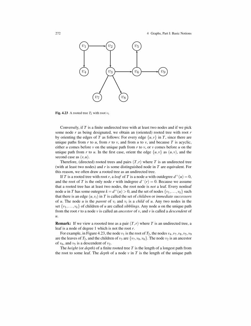
272 4 Graphs, Part I: Basic Notions
1
v2 v5v1
v4 v3 v6
v7 v8
v9
Fig. 4.23 A rooted tree T2 with root v1
Conversely, if T is a finite undirected tree with at least two nodes and if we picksome node r as being designated, we obtain an (oriented) rooted tree with root rby orienting the edges of T as follows: For every edge u,v in T , since there areunique paths from r to u, from r to v, and from u to v, and because T is acyclic,either u comes before v on the unique path from r to v, or v comes before u on theunique path from r to u. In the first case, orient the edge u,v as (u,v), and thesecond case as (v,u).
Therefore, (directed) rooted trees and pairs (T,r) where T is an undirected tree(with at least two nodes) and r is some distinguished node in T are equivalent. Forthis reason, we often draw a rooted tree as an undirected tree.
If T is a rooted tree with root r, a leaf of T is a node u with outdegree d+(u) = 0,and the root of T is the only node r with indegree d−(r) = 0. Because we assumethat a rooted tree has at least two nodes, the root node is not a leaf. Every nonleafnode u in T has some outegree k = d+(u)> 0, and the set of nodes v1, . . . ,vk suchthat there is an edge (u,vi) in T is called the set of children or immediate successorsof u. The node u is the parent of vi and vi is a child of u. Any two nodes in theset v1, . . . ,vk of children of u are called sibblings. Any node u on the unique pathfrom the root r to a node v is called an ancestor of v, and v is called a descendent ofu.
Remark: If we view a roooted tree as a pair (T,r) where T is an undirected tree, aleaf is a node of degree 1 which is not the root r.
For example, in Figure 4.23, the node v1 is the root of T2, the nodes v4,v7,v8,v5,v9are the leaves of T2, and the children of v3 are v7,v8,v6. The node v2 is an ancestorof v6, and v5 is a descendent of v2.
The height (or depth) of a finite rooted tree T is the length of a longest path fromthe root to some leaf. The depth of a node v in T is the length of the unique path
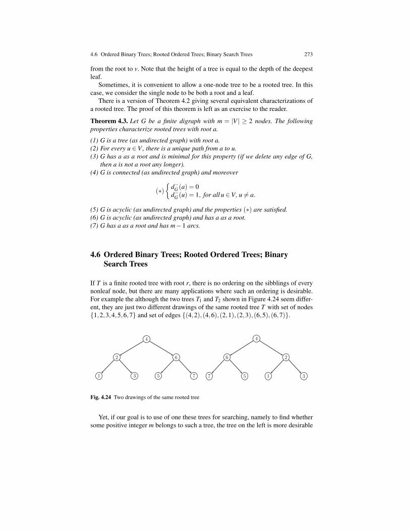
4.6 Ordered Binary Trees; Rooted Ordered Trees; Binary Search Trees 273
from the root to v. Note that the height of a tree is equal to the depth of the deepestleaf.
Sometimes, it is convenient to allow a one-node tree to be a rooted tree. In thiscase, we consider the single node to be both a root and a leaf.
There is a version of Theorem 4.2 giving several equivalent characterizations ofa rooted tree. The proof of this theorem is left as an exercise to the reader.
Theorem 4.3. Let G be a finite digraph with m = |V | ≥ 2 nodes. The followingproperties characterize rooted trees with root a.
(1) G is a tree (as undirected graph) with root a.(2) For every u ∈V , there is a unique path from a to u.(3) G has a as a root and is minimal for this property (if we delete any edge of G,
then a is not a root any longer).(4) G is connected (as undirected graph) and moreover
(∗)
d−G (a) = 0d−G (u) = 1, for all u ∈V, u 6= a.
(5) G is acyclic (as undirected graph) and the properties (∗) are satisfied.(6) G is acyclic (as undirected graph) and has a as a root.(7) G has a as a root and has m−1 arcs.
4.6 Ordered Binary Trees; Rooted Ordered Trees; BinarySearch Trees
If T is a finite rooted tree with root r, there is no ordering on the sibblings of everynonleaf node, but there are many applications where such an ordering is desirable.For example the although the two trees T1 and T2 shown in Figure 4.24 seem differ-ent, they are just two different drawings of the same rooted tree T with set of nodes1,2,3,4,5,6,7 and set of edges (4,2),(4,6),(2,1),(2,3),(6,5),(6,7).
1 3 5 7
2 6
4
7 5 1 3
6 2
4
Fig. 4.24 Two drawings of the same rooted tree
Yet, if our goal is to use of one these trees for searching, namely to find whethersome positive integer m belongs to such a tree, the tree on the left is more desirable
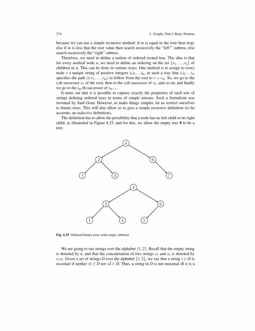
274 4 Graphs, Part I: Basic Notions
because we can use a simple recursive method: if m is equal to the root then stop;else if m is less that the root value then search recursively the “left”’ subtree, elsesearch recursively the “right” subtree.
Therefore, we need to define a notion of ordered rooted tree. The idea is thatfor every nonleaf node u, we need to define an ordering on the set v1, . . . ,vk ofchildren or u. This can be done in various ways. One method is to assign to everynode v a unique string of positive integers i1i2 . . . im, in such a way that i1i2 . . . imspecifies the path (r,v1, . . . ,vm) to follow from the root to v = vm. So, we go to thei1th successor v1 of the root, then to the i2th successor of v1, and so on, and finallywe go to the im-th successor of vm−1.
It turns out that it is possible to capture exactly the properties of such sets ofstrings defining ordered trees in terms of simple axioms. Such a formalism wasinvented by Saul Gorn. However, to make things simpler, let us restrict ourselvesto binary trees. This will also allow us to give a simple recursive definition (to beaccurate, an inductive definition).
The definition has to allow the possibility that a node has no left child or no rightchild, as illustrated in Figure 4.25, and for this, we allow the empty tree /0 to be atree.
1 3 7
2 6
4
1 3 5
2 6
4
Fig. 4.25 Ordered binary trees with empty subtrees
We are going to use strings over the alphabet 1,2. Recall that the empty stringis denoted by ε , and that the concatenation of two strings s1 and s2 is denoted bys1s2. Given a set of strings D over the alphabet 1,2, we say that a string s ∈ D ismaximal if neither s1 ∈ D nor s2 ∈ D. Thus, a string in D is not maximal iff it is a
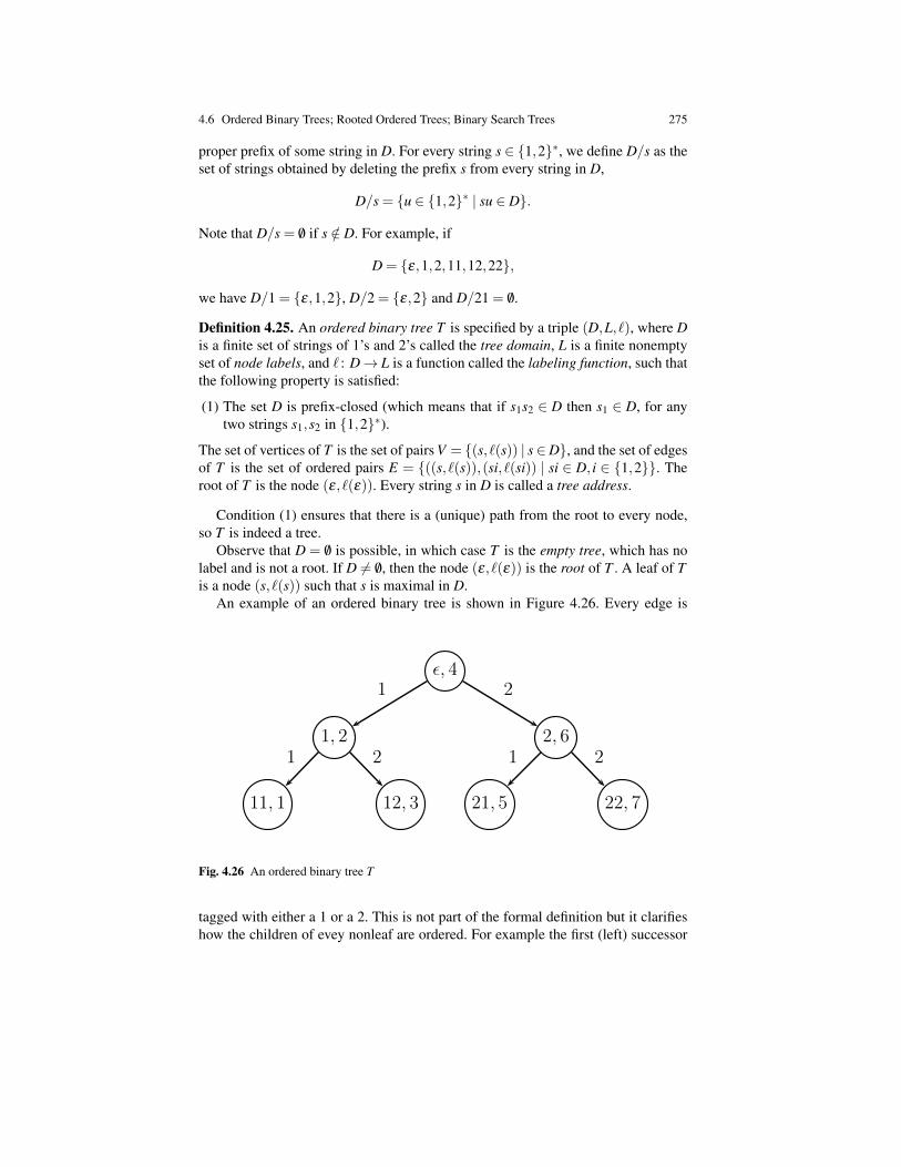
4.6 Ordered Binary Trees; Rooted Ordered Trees; Binary Search Trees 275
proper prefix of some string in D. For every string s ∈ 1,2∗, we define D/s as theset of strings obtained by deleting the prefix s from every string in D,
D/s = u ∈ 1,2∗ | su ∈ D.
Note that D/s = /0 if s /∈ D. For example, if
D = ε,1,2,11,12,22,
we have D/1 = ε,1,2, D/2 = ε,2 and D/21 = /0.
Definition 4.25. An ordered binary tree T is specified by a triple (D,L, `), where Dis a finite set of strings of 1’s and 2’s called the tree domain, L is a finite nonemptyset of node labels, and ` : D→ L is a function called the labeling function, such thatthe following property is satisfied:
(1) The set D is prefix-closed (which means that if s1s2 ∈ D then s1 ∈ D, for anytwo strings s1,s2 in 1,2∗).
The set of vertices of T is the set of pairs V = (s, `(s)) | s∈D, and the set of edgesof T is the set of ordered pairs E = ((s, `(s)),(si, `(si)) | si ∈ D, i ∈ 1,2. Theroot of T is the node (ε, `(ε)). Every string s in D is called a tree address.
Condition (1) ensures that there is a (unique) path from the root to every node,so T is indeed a tree.
Observe that D = /0 is possible, in which case T is the empty tree, which has nolabel and is not a root. If D 6= /0, then the node (ε, `(ε)) is the root of T . A leaf of Tis a node (s, `(s)) such that s is maximal in D.
An example of an ordered binary tree is shown in Figure 4.26. Every edge is
11, 1 12, 3 21, 5 22, 7
1, 2 2, 6
!, 41 2
1 2 1 2
Fig. 4.26 An ordered binary tree T
tagged with either a 1 or a 2. This is not part of the formal definition but it clarifieshow the children of evey nonleaf are ordered. For example the first (left) successor

276 4 Graphs, Part I: Basic Notions
of node (ε,4) is (1,2), and the second (right) successor of (ε,4) is (2,6). For everynode (s,u), the string s specifies which path to follow from the root to that node.For example, if we consider the node (21,5), the string 21 indicates that from theroot, we first have to go to the second child, and then to the first child of that node.In order to implement such trees, we can replace each nonleaf node (s,u) by a node(l,r,u), where l is a pointer to the left child (s1,v1) of (s,u) if it exists, r is a pointerto the right child (s2,v2) of (s,u) if it exists, and otherwise l (or r) is the specialpointer nil (or /0).
Figure 4.27 shows examples of ordered binary trees with some empty subtrees.
11, 1 12, 3 22, 7
1, 2 2, 6
!, 41 2
1 2 2
11, 1 12, 3 21, 5
1, 2 2, 6
!, 41 2
1 2 1
Fig. 4.27 Ordered binary trees with some empty subtrees
An ordered binary tree is a special kind of positional tree for which every nonleafnode has exactly two successors, one which may be the empty subtree (but not both);see Cormen, Leiserson, Rivest and Stein [3], Appendix B.5.3.
One should be aware that defining ordered binary trees requires more than draw-ing pictures in which some implicit left-to-right ordering is assumed. If we drawtrees upside-down (as is customary) with the root at the top and the leaves at thebottom, then we can indeed rely on the left-to-right ordering. However, if we drawtrees as they grow in nature (which is the case for proof trees used in logic), withthe root at the bottom and the leaves at the top, then we have rotated our trees by180 degrees, and left has become right and vice-versa! The definition in terms oftree addresses does not rely on drawings. By definition, the left child (if it exists) ofa node (s,u) is (s1,v1), and the right child (if it exists) of node (s,u) is (s2,v2).
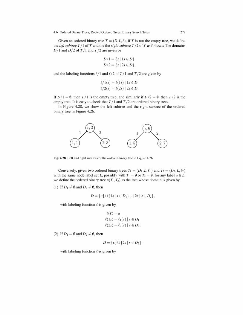
4.6 Ordered Binary Trees; Rooted Ordered Trees; Binary Search Trees 277
Given an ordered binary tree T = (D,L, `), if T is not the empty tree, we definethe left subtree T/1 of T and the the right subtree T/2 of T as follows: The domainsD/1 and D/2 of T/1 and T/2 are given by
D/1 = s | 1s ∈ DD/2 = s | 2s ∈ D,
and the labeling functions `/1 and `/2 of T/1 and T/2 are given by
`/1(s) = `(1s) | 1s ∈ D
`/2(s) = `(2s) | 2s ∈ D.
If D/1 = /0, then T/1 is the empty tree, and similarly if D/2 = /0, then T/2 is theempty tree. It is easy to check that T/1 and T/2 are ordered binary trees.
In Figure 4.28, we show the left subtree and the right subtree of the orderedbinary tree in Figure 4.26.
1, 1 2, 3
!, 21 2
1, 5 2, 7
!, 61 2
Fig. 4.28 Left and right subtrees of the ordered binary tree in Figure 4.26
Conversely, given two ordered binary trees T1 = (D1,L, `1) and T2 = (D2,L, `2)with the same node label set L, possibly with T1 = /0 or T2 = /0, for any label u ∈ L,we define the ordered binary tree u(T1,T2) as the tree whose domain is given by
(1) If D1 6= /0 and D2 6= /0, then
D = ε∪1s | s ∈ D1∪2s | s ∈ D2,
with labeling function ` is given by
`(ε) = u
`(1s) = `1(s) | s ∈ D1
`(2s) = `2(s) | s ∈ D2;
(2) If D1 = /0 and D2 6= /0, then
D = ε∪2s | s ∈ D2,
with labeling function ` is given by
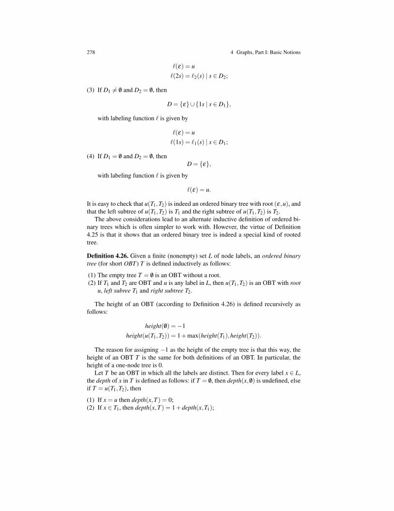
278 4 Graphs, Part I: Basic Notions
`(ε) = u
`(2s) = `2(s) | s ∈ D2;
(3) If D1 6= /0 and D2 = /0, then
D = ε∪1s | s ∈ D1,
with labeling function ` is given by
`(ε) = u
`(1s) = `1(s) | s ∈ D1;
(4) If D1 = /0 and D2 = /0, thenD = ε,
with labeling function ` is given by
`(ε) = u.
It is easy to check that u(T1,T2) is indeed an ordered binary tree with root (ε,u), andthat the left subtree of u(T1,T2) is T1 and the right subtree of u(T1,T2) is T2.
The above considerations lead to an alternate inductive definition of ordered bi-nary trees which is often simpler to work with. However, the virtue of Definition4.25 is that it shows that an ordered binary tree is indeed a special kind of rootedtree.
Definition 4.26. Given a finite (nonempty) set L of node labels, an ordered binarytree (for short OBT) T is defined inductively as follows:
(1) The empty tree T = /0 is an OBT without a root.(2) If T1 and T2 are OBT and u is any label in L, then u(T1,T2) is an OBT with root
u, left subree T1 and right subtree T2.
The height of an OBT (according to Definition 4.26) is defined recursively asfollows:
height( /0) =−1height(u(T1,T2)) = 1+max(height(T1),height(T2)).
The reason for assigning −1 as the height of the empty tree is that this way, theheight of an OBT T is the same for both definitions of an OBT. In particular, theheight of a one-node tree is 0.
Let T be an OBT in which all the labels are distinct. Then for every label x ∈ L,the depth of x in T is defined as follows: if T = /0, then depth(x, /0) is undefined, elseif T = u(T1,T2), then
(1) If x = u then depth(x,T ) = 0;(2) If x ∈ T1, then depth(x,T ) = 1+depth(x,T1);

4.6 Ordered Binary Trees; Rooted Ordered Trees; Binary Search Trees 279
(3) If x ∈ T2, then depth(x,T ) = 1+depth(x,T2);(4) If x /∈ T , then depth(x,T ) is undefined.
If T = u(T1,T2) is a nonempty OBT, then observe that
height(T1)< height(u(T1,T2)) and height(T2)< height(u(T1,T2)).
Thus, in order to prove properties of OBTs we can proceed by induction on theheight of trees, which yields the following extremely useful induction principlecalled structural induction principle.
Structural Induction Principle for OBTs
Let P be a property of OBTs. If
(1) P( /0) holds (base case), and(2) Whenever P(T1) and P(T2) hold, then P(u(T1,T2)) holds (induction step),
then P(T ) holds for all OBTs T .
The OBTs given by Definition 4.26 are reallly symbolic representations of theOBTs given by Definition 4.25. There is a bijective correspondence E between theset of OBTs given by Definition 4.25 and the set of OBTs given by Definition 4.26.Namely,
E ( /0) = /0,
and for any nonempty OBT T with root (ε,u), if T1 and T2 are the left and rightsubtrees of T , then
E (T ) = u(E (T1),E (T2)).
Observe that the one-node rooted ordered tree with node label u is represented byE (u) = u( /0, /0). Using structural induction, it is not hard to show that for every in-ductively defined OBT T ′, there is a unique OBT T such that E (T ) = T ′. Therefore,E is indeed a bijection.
When drawing OBTs defined according to Definition 4.26, it is customary toomit all empty subtrees. The binary ordered tree T shown at the top of Figure 4.29is mapped to the OBT shown at the bottom of Figure 4.29. Similarly, the binaryordered tree shown at the top of Figure 4.30 is mapped to the OBT shown at thebottom of Figure 4.30.
We say that a nonempty OBT T is complete if either T = u( /0, /0), or T = u(T1,T2)where both T1 and T2 are complete OBTs of the same height. If T is a nonemptyOBT of height h and if all its labels are distinct, then it is easy to show that Tis complete iff all leaves are at depth h and if all nonleaf nodes have exactly twochildren. The following proposition is easy to show.
Proposition 4.9. For any nonempty OBT T , if T has height h, then
(1) T has at most 2h+1−1 nodes.(2) T has at most 2h leaves.
Both maxima are achieved by complete OBTs.

280 4 Graphs, Part I: Basic Notions
11, 1 12, 3 21, 5 22, 7
1, 2 2, 6
!, 41 2
1 2 1 2
1 3 5 7
2 6
4
Fig. 4.29 An ordered binary tree; top, Definition 4.25; bottom, Definition 4.26
11, 1 12, 3 21, 5
1, 2 2, 6
!, 41 2
1 2 1
1 3 5
2 6
4
Fig. 4.30 An ordered binary tree; top, Definition 4.25; bottom, Definition 4.26
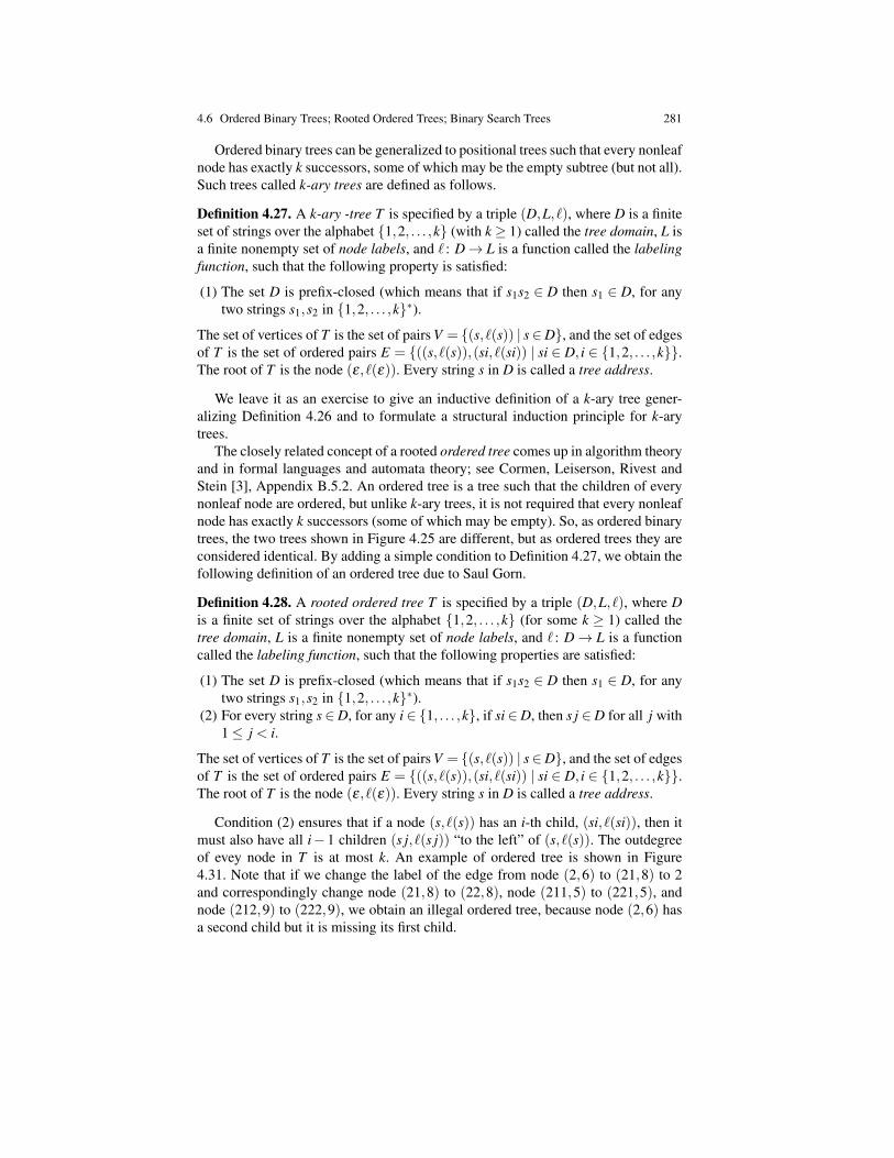
4.6 Ordered Binary Trees; Rooted Ordered Trees; Binary Search Trees 281
Ordered binary trees can be generalized to positional trees such that every nonleafnode has exactly k successors, some of which may be the empty subtree (but not all).Such trees called k-ary trees are defined as follows.
Definition 4.27. A k-ary -tree T is specified by a triple (D,L, `), where D is a finiteset of strings over the alphabet 1,2, . . . ,k (with k≥ 1) called the tree domain, L isa finite nonempty set of node labels, and ` : D→ L is a function called the labelingfunction, such that the following property is satisfied:
(1) The set D is prefix-closed (which means that if s1s2 ∈ D then s1 ∈ D, for anytwo strings s1,s2 in 1,2, . . . ,k∗).
The set of vertices of T is the set of pairs V = (s, `(s)) | s∈D, and the set of edgesof T is the set of ordered pairs E = ((s, `(s)),(si, `(si)) | si ∈ D, i ∈ 1,2, . . . ,k.The root of T is the node (ε, `(ε)). Every string s in D is called a tree address.
We leave it as an exercise to give an inductive definition of a k-ary tree gener-alizing Definition 4.26 and to formulate a structural induction principle for k-arytrees.
The closely related concept of a rooted ordered tree comes up in algorithm theoryand in formal languages and automata theory; see Cormen, Leiserson, Rivest andStein [3], Appendix B.5.2. An ordered tree is a tree such that the children of everynonleaf node are ordered, but unlike k-ary trees, it is not required that every nonleafnode has exactly k successors (some of which may be empty). So, as ordered binarytrees, the two trees shown in Figure 4.25 are different, but as ordered trees they areconsidered identical. By adding a simple condition to Definition 4.27, we obtain thefollowing definition of an ordered tree due to Saul Gorn.
Definition 4.28. A rooted ordered tree T is specified by a triple (D,L, `), where Dis a finite set of strings over the alphabet 1,2, . . . ,k (for some k ≥ 1) called thetree domain, L is a finite nonempty set of node labels, and ` : D→ L is a functioncalled the labeling function, such that the following properties are satisfied:
(1) The set D is prefix-closed (which means that if s1s2 ∈ D then s1 ∈ D, for anytwo strings s1,s2 in 1,2, . . . ,k∗).
(2) For every string s ∈D, for any i ∈ 1, . . . ,k, if si ∈D, then s j ∈D for all j with1≤ j < i.
The set of vertices of T is the set of pairs V = (s, `(s)) | s∈D, and the set of edgesof T is the set of ordered pairs E = ((s, `(s)),(si, `(si)) | si ∈ D, i ∈ 1,2, . . . ,k.The root of T is the node (ε, `(ε)). Every string s in D is called a tree address.
Condition (2) ensures that if a node (s, `(s)) has an i-th child, (si, `(si)), then itmust also have all i− 1 children (s j, `(s j)) “to the left” of (s, `(s)). The outdegreeof evey node in T is at most k. An example of ordered tree is shown in Figure4.31. Note that if we change the label of the edge from node (2,6) to (21,8) to 2and correspondingly change node (21,8) to (22,8), node (211,5) to (221,5), andnode (212,9) to (222,9), we obtain an illegal ordered tree, because node (2,6) hasa second child but it is missing its first child.
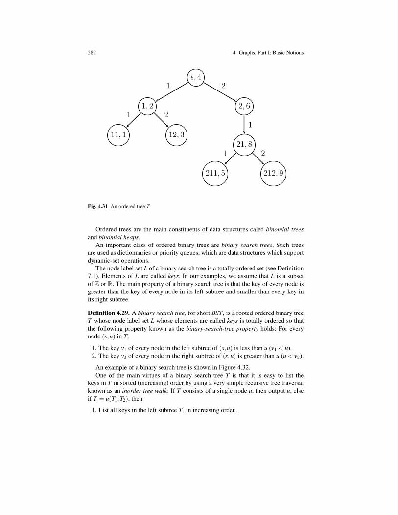
282 4 Graphs, Part I: Basic Notions
11, 1 12, 3
211, 5 212, 9
1, 2
21, 8
2, 6
!, 41 2
1 2
1 2
1
Fig. 4.31 An ordered tree T
Ordered trees are the main constituents of data structures caled binomial treesand binomial heaps.
An important class of ordered binary trees are binary search trees. Such treesare used as dictionnaries or priority queues, which are data structures which supportdynamic-set operations.
The node label set L of a binary search tree is a totally ordered set (see Definition7.1). Elements of L are called keys. In our examples, we assume that L is a subsetof Z or R. The main property of a binary search tree is that the key of every node isgreater than the key of every node in its left subtree and smaller than every key inits right subtree.
Definition 4.29. A binary search tree, for short BST , is a rooted ordered binary treeT whose node label set L whose elements are called keys is totally ordered so thatthe following property known as the binary-search-tree property holds: For everynode (s,u) in T ,
1. The key v1 of every node in the left subtree of (s,u) is less than u (v1 < u).2. The key v2 of every node in the right subtree of (s,u) is greater than u (u < v2).
An example of a binary search tree is shown in Figure 4.32.One of the main virtues of a binary search tree T is that it is easy to list the
keys in T in sorted (increasing) order by using a very simple recursive tree traversalknown as an inorder tree walk: If T consists of a single node u, then output u; elseif T = u(T1,T2), then
1. List all keys in the left subtree T1 in increasing order.

4.6 Ordered Binary Trees; Rooted Ordered Trees; Binary Search Trees 283
2. List u.3. List all keys in the right subtree T2 in increasing order.
2 4 13
17 203 7
18
15
6
9
Fig. 4.32 A binary seach tree
Other simple queries are easily performed on binary search trees. These are
1. Search for a key.2. Find the minimum key.3. Find the maximum key.4. Find the predecessor of a key.5. Find the successor of a key.
Given a BST tree T and given a key v, to find whether v is equal to some key inT we can proceed recursively as follows: If T = u(T1,T2) then
1. If v = u, then return v.2. if v 6= u and T1 = T2 = /0, then return v not found.3. If v 6= u and T1 6= /0 or T2 6= /0, then
a. if v < u then search for v in the left subtree T1,b. else search for v in the right subtree T2.
It is easy to modify the above function to return the node containing the key v ifv occurs in T .
To find the minimum key in T , recursively follow the left pointer of every node(that is, recursively go down the left subtree). For example, in the BST of Figure

284 4 Graphs, Part I: Basic Notions
4.32 following left links starting from the root node 15, we reach the “leftmost” leaf2.
To find the maximum key in T , recursively follow the right pointer of every node(that is, recursively go down the right subtree). For example, in the BST of Figure4.32 following right links starting from the root node 15, we reach the “rightmost”leaf 20.
In order to find the successor of the key u associated with a node (s,u), we needto consider two cases:
1. If (s,u) has a nonempty right subtree T2, then the successor of u is the key v ofthe leftmost node in the subtree T2, which is found by recursively following theleft links of the root of T2 (as in the case of finding the minimum key).
2. If (s,u) has an empty right subtree, then we need to go up along a path to theroot, and find the lowest ancestor of (s,u) whose left child is also an ancestor of(s,u).
For example, in the BST of Figure 4.32, the successor of 15 is 17, and the succes-sor of 13 is 15. We leave it as an exercise to prove that the above method is correct.Finding the predecessor of a key is symmetric to the method for finding a successor.
Other operations on BST can be easily performed, such as
1. Inserting a node (containing a new key).2. Deleting a node.
In both cases, we have to make sure that the binary-search-tree property is pre-served. Inserting a new key is done recursively and easy to do. Deleting a node isa bit more subtle because it depends on the number of children of the node to bedeleted. These operations are described in any algorithms course and will not bediscussed here.
Of course, as soon as we allow performing insertions of deletions of nodes in aBST, it is possible to obtain “unbalanced” BSTs (namely, BSTs with large height)and the cost of performing operations on such unbalanced trees becomes greater.Therefore, it may be desirable to perform operations to rebalance BSTs known asrotations. There is a particular class of BSTs known as red-black trees that keepBSTs well balanced. Again, these are described in any algorithms course. An excel-lent source is Cormen, Leiserson, Rivest and Stein [3].
Before closing this section, let us mention another kind of data structure usingordered binary trees, namely a binary heap. A heap does not satisfy the binary-search-tree property but instead a heap property, which is one of the following twoproperties:
1. The min-heap-property, which says that for every node (s,u) in the heap H, thekey of every descendent of (s,u) is greater than u.
2. The max-heap-property, which says that for every node (s,u) in the heap H, thekey of every descendent of (s,u) is smaller than u.
Thus, in a heap satisfying the min-heap-property, the smallest key is at the root,and in a heap satisfying the max-heap-property, the largest key is at the root. A
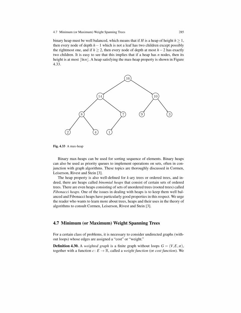
4.7 Minimum (or Maximum) Weight Spanning Trees 285
binary heap must be well balanced, which means that if H is a heap of height h≥ 1,then every node of depth h−1 which is not a leaf has two children except possiblythe rightmost one, and if h ≥ 2, then every node of depth at most h−2 has exactlytwo children. It is easy to see that this implies that if a heap has n nodes, then itsheight is at most blnnc. A heap satisfying the max-heap property is shown in Figure4.33.
2 4 1
9 38 7
10
16
14
Fig. 4.33 A max-heap
Binary max-heaps can be used for sorting sequence of elements. Binary heapscan also be used as priority queues to implement operations on sets, often in con-junction with graph algorithms. These topics are thoroughly discussed in Cormen,Leiserson, Rivest and Stein [3].
The heap property is also well-defined for k-ary trees or ordered trees, and in-deed, there are heaps called binomial heaps that consist of certain sets of orderedtrees. There are even heaps consisting of sets of unordered trees (rooted trees) calledFibonacci heaps. One of the issues in dealing with heaps is to keep them well bal-anced and Fibonacci heaps have particularly good properties in this respect. We urgethe reader who wants to learn more about trees, heaps and their uses in the theory ofalgorithms to consult Cormen, Leiserson, Rivest and Stein [3].
4.7 Minimum (or Maximum) Weight Spanning Trees
For a certain class of problems, it is necessary to consider undirected graphs (with-out loops) whose edges are assigned a “cost” or “weight.”
Definition 4.30. A weighted graph is a finite graph without loops G = (V,E,st),together with a function c : E → R, called a weight function (or cost function). We
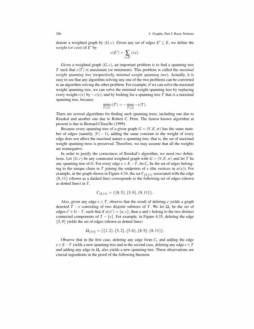
286 4 Graphs, Part I: Basic Notions
denote a weighted graph by (G,c). Given any set of edges E ′ ⊆ E, we define theweight (or cost) of E ′ by
c(E ′) = ∑e∈E ′
c(e).
Given a weighted graph (G,c), an important problem is to find a spanning treeT such that c(T ) is maximum (or minimum). This problem is called the maximalweight spanning tree (respectively, minimal weight spanning tree). Actually, it iseasy to see that any algorithm solving any one of the two problems can be convertedto an algorithm solving the other problem. For example, if we can solve the maximalweight spanning tree, we can solve the minimal weight spanning tree by replacingevery weight c(e) by −c(e), and by looking for a spanning tree T that is a maximalspanning tree, because
minT⊆G
c(T ) =−maxT⊆G−c(T ).
There are several algorithms for finding such spanning trees, including one due toKruskal and another one due to Robert C. Prim. The fastest known algorithm atpresent is due to Bernard Chazelle (1999).
Because every spanning tree of a given graph G = (V,E,st) has the same num-ber of edges (namely, |V | − 1), adding the same constant to the weight of everyedge does not affect the maximal nature a spanning tree, that is, the set of maximalweight spanning trees is preserved. Therefore, we may assume that all the weightsare nonnegative.
In order to justify the correctness of Kruskal’s algorithm, we need two defini-tions. Let (G,c) be any connected weighted graph with G = (V,E,st) and let T beany spanning tree of G. For every edge e ∈ E−T , let Ce be the set of edges belong-ing to the unique chain in T joining the endpoints of e (the vertices in st(e)). Forexample, in the graph shown in Figure 4.34, the set C8,11 associated with the edge8,11 (shown as a dashed line) corresponds to the following set of edges (shownas dotted lines) in T ,
C8,11 = 8,5,5,9,9,11.
Also, given any edge e ∈ T , observe that the result of deleting e yields a graphdenoted T − e consisting of two disjoint subtrees of T . We let Ωe be the set ofedges e′ ∈G−T , such that if st(e′) = u,v, then u and v belong to the two distinctconnected components of T −e. For example, in Figure 4.35, deleting the edge5,9 yields the set of edges (shown as dotted lines)
Ω5,9 = 1,2,5,2,5,6,8,9,8,11.
Observe that in the first case, deleting any edge from Ce and adding the edgee∈ E−T yields a new spanning tree and in the second case, deleting any edge e∈ Tand adding any edge in Ωe also yields a new spanning tree. These observations arecrucial ingredients in the proof of the following theorem.

4.7 Minimum (or Maximum) Weight Spanning Trees 287
1
1 2 3
4 5 6 7
8 9 10
11 12
Fig. 4.34 The set Ce associated with an edge e ∈ G−T
1
1 2 3
4 5 6 7
8 9 10
11 12
Fig. 4.35 The set Ω5,9 obtained by deleting the edge 5,9 from the spanning tree.

288 4 Graphs, Part I: Basic Notions
Theorem 4.4. Let (G,c) be any connected weighted graph and let T be any span-ning tree of G. (1) The tree T is a maximal weight spanning tree iff any of thefollowing (equivalent) conditions hold.
(i) For every e ∈ E−T ,c(e)≤ min
e′∈Cec(e′)
(ii) For every e ∈ T ,c(e)≥ max
e′∈Ωec(e′).
(2) The tree T is a minimal weight spanning tree iff any of the following (equiv-alent) conditions hold.
(i) For every e ∈ E−T ,c(e)≥ max
e′∈Cec(e′)
(ii) For every e ∈ T ,c(e)≤ min
e′∈Ωec(e′).
Proof . (1) First, assume that T is a maximal weight spanning tree. Observe that
(a) For any e∈E−T and any e′ ∈Ce, the graph T ′= (V,(T ∪e)−e′) is acyclicand has |V |−1 edges, so it is a spanning tree. Then, (i) must hold, as otherwisewe would have c(T ′)> c(T ), contradicting the maximality of T .
(b) For any e∈ T and any e′ ∈Ωe, the graph T ′ = (V,(T ∪e′)−e) is connectedand has |V |−1 edges, so it is a spanning tree. Then, (ii) must hold, as otherwisewe would have c(T ′)> c(T ), contradicting the maximality of T .
Let us now assume that (i) holds. We proceed by contradiction. Let T be a span-ning tree satisfying condition (i) and assume there is another spanning tree T ′ withc(T ′) > c(T ). There are only finitely many spanning trees of G, therefore we mayassume that T ′ is maximal. Consider any edge e ∈ T ′−T and let st(e) = u,v. InT , there is a unique chain Ce joining u and v and this chain must contain some edgee′ ∈ T joining the two connected components of T ′−e; that is, e′ ∈Ωe. As (i) holds,we get c(e) ≤ c(e′). However, as T ′ is maximal, (ii) holds (as we just proved), soc(e)≥ c(e′). Therefore, we get
c(e) = c(e′).
Consequently, if we form the graph T2 = (T ′∪e′)−e), we see that T2 is a span-ning tree having some edge from T and c(T2) = c(T ′). We can repeat this processof edge substitution with T2 and T and so on. Ultimately, we obtain the tree T withthe weight c(T ′)> c(T ), which is absurd. Therefore, T is indeed maximal.
Finally, assume that (ii) holds. The proof is analogous to the previous proof: Wepick some edge e′ ∈ T −T ′ and e is some edge in Ωe′ belonging to the chain joiningthe endpoints of e′ in T ′.
(2) The proof of (2) is analogous to the proof of (1) but uses 2(i) and 2(ii) insteadof 1(i) and 1(ii). ut

4.7 Minimum (or Maximum) Weight Spanning Trees 289
We are now in the position to present a version of Kruskal’s algorithm and toprove its correctness.
Here is a version of Kruskal’s algorithm for finding a minimal weight spanningtree using criterion 2(i). Let n be the number of edges of the weighted graph (G,c),where G = (V,E,st).
Fig. 4.36 Joseph Kruskal, 1928–
function Kruskal((G,c): weighted graph): treebegin
Sort the edges in nondecreasing order of weights:c(e1)≤ c(e2)≤ ·· · ≤ c(en);T := /0;for i := 1 to n do
if (V,T ∪ei) is acyclic then T := T ∪eiendif
endfor;Kruskal := T
end
We admit that the above description of Kruskal’s algorithm is a bit sketchy as wehave not explicitly specified how we check that adding an edge to a tree preservesacyclicity. On the other hand, it is quite easy to prove the correctness of the abovealgorithm.
It is not difficult to refine the above “naive” algorithm to make it totally explicitbut this involves a good choice of data structures. We leave these considerations toan algorithms course.
Clearly, the graph T returned by the algorithm is acyclic, but why is it connected?Well, suppose T is not connected and consider two of its connected components, sayT1 and T2. Being acyclic and connected, T1 and T2 are trees. Now, as G itself is con-nected, for any node of T1 and any node of T2, there is some chain connecting thesenodes. Consider such a chain C, of minimal length. Then, as T1 is a tree, the firstedge e j of C cannot belong to T1 because otherwise we would get an even shorterchain connecting T1 and T2 by deleting e j. Furthermore, e j does not belong to any
290 4 Graphs, Part I: Basic Notions
other connected component of T , as these connected components are pairwise dis-joint. But then, T +e j is acyclic, which means that when we considered the additionof edge e j to the current graph T ( j), the test should have been positive and e j shouldhave been added to T ( j). Therefore, T is connected and so it is a spanning tree. Nowobserve that as the edges are sorted in nondecreasing order of weight, condition 2(i)is enforced and by Theorem 4.4, T is a minimal weight spanning tree.
We can easily design a version of Kruskal’s algorithm based on Condition 2(ii).This time, we sort the edges in nonincreasing order of weights and, starting with G,we attempt to delete each edge e j as long as the remaining graph is still connected.We leave the design of this algorithm as an exercise to the reader.
Prim’s algorithm is based on a rather different observation. For any node, v ∈V ,let Uv be the set of edges incident with v that are not loops,
Uv = e ∈ E | v ∈ st(e), st(e) ∈ [V ]2.
Choose in Uv some edge of minimum weight that we (ambiguously) denote by e(v).
Proposition 4.10. Let (G,c) be a connected weighted graph with G = (V,E,st). Forevery vertex v ∈V , there is a minimum weight spanning tree T so that e(v) ∈ T .
Proof . Let T ′ be a minimum weight spanning tree of G and assume that e(v) /∈ T ′.Let C be the chain in T ′ that joins the endpoints of e(v) and let e be the edge of Cthat is incident with v. Then, the graph T ′′ = (V,(T ′∪e(v))−e) is a spanningtree of weight less than or equal to the weight of T ′ and as T ′ has minimum weight,so does T ′′. By construction, e(v) ∈ T ′′. ut
Prim’s algorithm uses an edge-contraction operation described below:
Definition 4.31. Let G = (V,E,st) be a graph, and let e∈ E be some edge that is nota loop; that is, st(e) = u,v, with u 6= v. The graph Ce(G) obtained by contractingthe edge e is the graph obtained by merging u and v into a single node and deletinge. More precisely, Ce(G) = ((V −u,v)∪w,E−e,ste), where w is any newnode not in V and where
1. ste(e′) = st(e′) iff u /∈ st(e′) and v /∈ st(e′).2. ste(e′) = w,z iff st(e′) = u,z, with z /∈ st(e).3. ste(e′) = z,w iff st(e′) = z,v, with z /∈ st(e).4. ste(e′) = w iff st(e′) = u,v.
Proposition 4.11. Let G = (V,E,st) be a graph. For any edge, e ∈ E, the graph Gis a tree iff Ce(G) is a tree.
Proof . Proposition 4.11 follows from Theorem 4.2. Observe that G is connected iffCe(G) is connected. Moreover, if G is a tree, the number of nodes of Ce(G) is ne =|V |−1 and the number of edges of Ce(G) is me = |E|−1. Because |E|= |V |−1, weget me = ne−1 and Ce(G) is a tree. Conversely, if Ce(G) is a tree, then me = ne−1,|V |= ne +1 and |E|= me +1, so m = n−1 and G is a tree. ut
Here is a “naive” version of Prim’s algorithm.
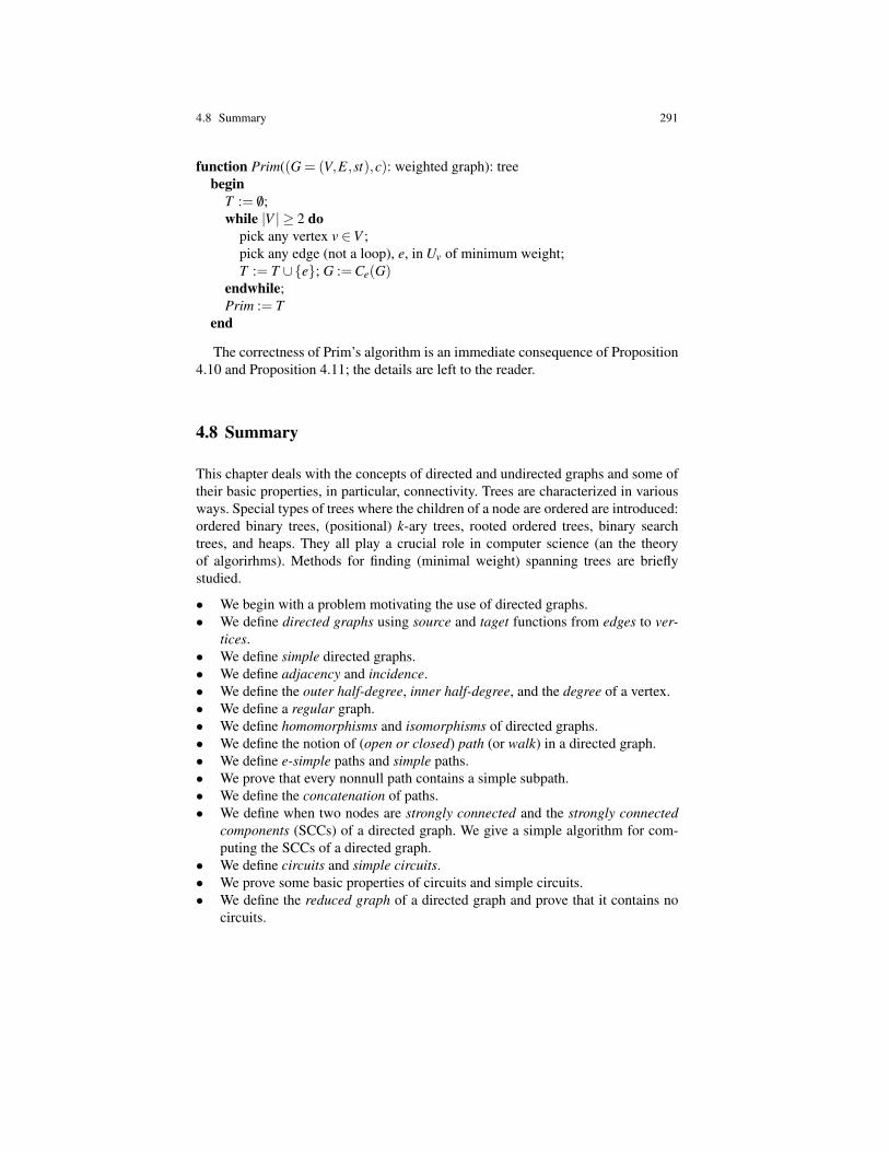
4.8 Summary 291
function Prim((G = (V,E,st),c): weighted graph): treebegin
T := /0;while |V | ≥ 2 do
pick any vertex v ∈V ;pick any edge (not a loop), e, in Uv of minimum weight;T := T ∪e; G :=Ce(G)
endwhile;Prim := T
end
The correctness of Prim’s algorithm is an immediate consequence of Proposition4.10 and Proposition 4.11; the details are left to the reader.
4.8 Summary
This chapter deals with the concepts of directed and undirected graphs and some oftheir basic properties, in particular, connectivity. Trees are characterized in variousways. Special types of trees where the children of a node are ordered are introduced:ordered binary trees, (positional) k-ary trees, rooted ordered trees, binary searchtrees, and heaps. They all play a crucial role in computer science (an the theoryof algorirhms). Methods for finding (minimal weight) spanning trees are brieflystudied.
• We begin with a problem motivating the use of directed graphs.• We define directed graphs using source and taget functions from edges to ver-
tices.• We define simple directed graphs.• We define adjacency and incidence.• We define the outer half-degree, inner half-degree, and the degree of a vertex.• We define a regular graph.• We define homomorphisms and isomorphisms of directed graphs.• We define the notion of (open or closed) path (or walk) in a directed graph.• We define e-simple paths and simple paths.• We prove that every nonnull path contains a simple subpath.• We define the concatenation of paths.• We define when two nodes are strongly connected and the strongly connected
components (SCCs) of a directed graph. We give a simple algorithm for com-puting the SCCs of a directed graph.
• We define circuits and simple circuits.• We prove some basic properties of circuits and simple circuits.• We define the reduced graph of a directed graph and prove that it contains no
circuits.

292 4 Graphs, Part I: Basic Notions
• We define subgraphs, induced subgraphs, spanning subgraphs, partial graphsand partial subgraphs.
• Next we consider undirected graphs.• We define a notion of undirected path called a chain.• We define e-simple chains and simple chains.• We define when two nodes are connected and the connected components of a
graph.• We define undirected circuits, called cycles and simple cycles• We define undirected graphs in terms of a function from the set of edges to the
union of the set of vertices and the set of two-element subsets of vertices.• We revisit the notion of chain in the framework of undirected graphs.• We define the degree of a node in an undirected graph.• We define the complete graph Kn on n vertices.• We state a version of Ramsey’s theorem and define Ramsey numbers.• We define homomorphisms and isomorphisms of undirected graphs.• We define the notion of a bridge in an undirected graph and give a characteriza-
tion of a bridge in terms of cycles.• We prove a basic relationship between the number of vertices and the number
of edges in a finite undirected graph G having to do with the fact that either Gis connected or G has no cycle.
• We define trees and forests.• We give several characterizations of a tree.• We prove that every connected graph possesses a spanning tree.• We define a leaf or endpoint.• We prove that every tree with at least two nodes has at least two leaves.• We define a root and an antiroot in a directed graph.• We define a rooted tree (or arborescence) (with a root or an antiroot).• We state a characterization of rooted trees.• We define rooted binary trees (OBTs) in two ways. The first definition uses
the notion of a tree domain and tree addresses. The second definition, which isinductive, yields a
• structural induction principle for ordered binary trees.• We define k-ary trees. These are positional trees generalizing OBTs.• We define rooted ordered trees.• We define binary search trees (BSTs) and discuss some operations on them.• We define the min-heap-property and the max-heap-property and briefly discuss
binary heaps.• We define (undirected) weighted graphs.• We prove a theorem characterizing maximal weight spanning trees (and minimal
weight spanning trees).• We present Kruskal’s algorithm for finding a minimal weight spanning tree.• We define edge contraction.• We present Prim’s algorithm for finding a minimal weight spanning tree.

4.8 Problems 293
Problems
4.1. (a) Give the list of all directed simple graphs with two nodes.(b) Give the list of all undirected simple graphs with two nodes.
4.2. Prove that in a party with an odd number of people, there is always a personwho knows an even number of others. Here we assume that the relation “knowing” issymmetric (i.e., if A knows B, then B knows A). Also, there may be pairs of peopleat the party who don’t know each other or even people who don’t know anybodyelse so “even” includes zero.
4.3. What is the maximum number of edges that an undirected simple graph with10 nodes can have?
4.4. Prove that every undirected simple graph with n≥ 2 nodes and more than(n−1)(n−2)/2 edges is connected.
4.5. If f : G1→G2 and g : G2→G3 are two graph homomorphisms, prove that theircomposition g f : G1→ G3 is also a graph homomorphism.
4.6. Prove that if f = ( f e, f v) is a graph isomorphism, then both f e and f v arebijections. Assume that f = ( f e, f v) is a graph homomorphism and that both f e andf v are bijections. Must f be a graph isomorphism?
4.7. If G1 and G2 are isomorphic finite directed graphs, then prove that for everyk ≥ 0, the number of nodes u in G1 such that d−G1
(u) = k, is equal to the number ofnodes v ∈ G2, such that d−G2
(v) = k (respectively, the number of nodes u in G1 suchthat d+
G1(u) = k, is equal to the number of nodes v ∈G2, such that d+
G2(v) = k). Give
a counterexample showing that the converse property is false.
4.8. Prove that every undirected simple graph with at least two nodes has two nodeswith the same degree.
4.9. If G = (V,E) is an undirected simple graph, prove that E can be partitioned intosubsets of edges corresponding to simple cycles if and only if every vertex has evendegree.
4.10. Let G = (V,E) be an undirected simple graph. Prove that if G has n nodes andif |E|> bn2/4c, then G contains a triangle.Hint. Proceed by contradiction. First, prove that for every edge u,v ∈ E,
d(u)+d(v)≤ n,
and use this to prove that∑u∈V
d(u)2 ≤ n|E|.
Finally, use the Cauchy–Schwarz inequality.

294 4 Graphs, Part I: Basic Notions
4.11. Given any undirected simple graph G = (V,E) with at least two vertices, forany vertex u ∈V , denote by G−u the graph obtained from G by deleting the vertexu from V and deleting from E all edges incident with u. Prove that if G is connected,then there are two distinct vertices u,v in V such that G−u and G−v are connected.
4.12. Given any undirected simple graph G = (V,E) with at least one vertex, let
δ (G) = mind(v) | v ∈V
be the minimum degree of G, let
ε(G) =|E||V | ,
and letd(G) =
1|V | ∑v∈V
d(v)
be the average degree of G. Prove that δ (G)≤ d(G) and
ε(G) =12
d(G).
Prove that if G has at least one edge, then G has a subgraph H such that
δ (H)> ε(H)≥ ε(G).
4.13. For any undirected simple graph G = (V,E), prove that if δ (G) ≥ 2 (whereδ (G) is the minimun degree of G as defined in Problem 4.12), then G contains asimple chain of length at least δ (G) and a simple cycle of length at least δ (G)+1.
4.14. An undirected graph G is h-connected (h ≥ 1) iff the result of deleting anyh− 1 vertices and the edges adjacent to these vertices does not disconnect G. Anarticulation point u in G is a vertex whose deletion increases the number of con-nected components. Prove that if G has n ≥ 3 nodes, then the following propertiesare equivalent.
(1) G is 2-connected.(2) G is connected and has no articulation point.(3) For every pair of vertices (u,v) in G, there is a simple cycle passing through u
and v.(4) For every vertex u in G and every edge e ∈ G, there is a simple cycle passing
through u containing e.(5) For every pair of edges (e, f ) in G, there is a simple cycle containing e and f .(6) For every triple of vertices (a,b,c) in G, there is a chain from a to b passing
through c.(7) For every triple of vertices (a,b,c) in G, there is a chain from a to b not passing
through c.
4.8 Problems 295
4.15. Give an algorithm for finding the connected components of an undirected fi-nite graph.
4.16. If G = (V,E) is an undirected simple graph, then its complement is the graph,G = (V,E); that is, an edge, u,v, is an edge of G iff it is not an edge of G.
(a) Prove that either G or G is connected.(b) Give an example of an undirected simple graph with four nodes that is iso-
morphic to its complement.(c) Give an example of an undirected simple graph with five nodes that is iso-
morphic to its complement.(d) Give an example of an undirected simple graph with nine nodes that is iso-
morphic to its complement.(e) Prove that if an undirected simple graph with n nodes is isomorphic to its
complement, then either n≡ 0 (mod 4) or n≡ 1 (mod 4).
4.17. Let G = (V,E) be any undirected simple graph. A clique is any subset S of Vsuch that any two distinct vertices in S are adjacent; equivalently, S is a clique if thesubgraph of G induced by S is a complete graph. The clique number of G, denotedby ω(G), is the size of a largest clique. An independent set is any subset S of V suchthat no two distinct vertices in S are adjacent; equivalently, S is an independent setif the subgraph of G induced by S has no edges. The independence number of G,denoted by α(G), is the size of a largest independent set.
(a) If G is the complement of the graph G (as defined in Problem 4.16), provethat
ω(G) = α(G), α(G) = ω(G).
(b) Prove that if V has at least six vertices, then either ω(G)≥ 3 or ω(G)≥ 3.
4.18. Let G = (V,E) be an undirected graph. Let E ′ be the set of edges in any cyclein G. Then, every vertex of the partial graph (V,E ′) has even degree.
4.19. A directed graph G is quasi-strongly connected iff for every pair of nodes(a,b) there is some node c in G such that there is a path from c to a and a path fromc to b. Prove that G is quasi-strongly connected iff G has a root.
4.20. A directed graph G = (V,E,s, t) is
1. Injective iff d−G (u)≤ 1, for all u ∈V .2. Functional iff d+
G (u)≤ 1, for all u ∈V .
(a) Prove that an injective graph is quasi-strongly connected iff it is connected(as an undirected graph).
(b) Prove that an undirected simple graph G can be oriented to form either aninjective graph or a functional graph iff every connected component of G has atmost one cycle.
4.21. Design a version of Kruskal’s algorithm based on condition 2(ii) of Theorem4.4.
296 4 Graphs, Part I: Basic Notions
4.22. (a) List all (unoriented) trees with four nodes and then five nodes.(b) Recall that the complete graph Kn with n vertices (n≥ 2) is the simple undi-
rected graph whose edges are all two-element subsets i, j, with i, j ∈ 1,2, . . . ,nand i 6= j. List all spanning trees of the complete graphs K2 (one tree), K3 (3 trees),and K4 (16 trees).
Remark: It can be shown that the number of spanning trees of Kn is nn−2, a formuladue to Cayley (1889); see Problem 5.38.
4.23. Prove that the graph K5 with the coloring shown on Figure 4.19 (left) does notcontain any complete subgraph on three vertices whose edges are all of the samecolor. Prove that for every edge coloring of the graph K6 using two colors (say redand blue), there is a complete subgraph on three vertices whose edges are all of thesame color.
References
1. Claude Berge. Graphs and Hypergraphs. Amsterdam: Elsevier North-Holland, first edition,1973.
2. Bela Bollobas. Modern Graph Theory. GTM No. 184. New York: Springer Verlag, firstedition, 1998.
3. Thomas Cormen, Charles Leiserson, Ronald Rivest, Clifford Stein. Introduction to Algo-rithms. Cambridge, MA: McGraw-Hill, second edition, 2001.
4. Reinhard Diestel. Graph Theory. GTM No. 173. New York: Springer Verlag, third edition,2005.
5. Frank Harary. Graph Theory. Reading, MA: Addison Wesley, first edition, 1971.6. Michel Sakarovitch. Optimisation Combinatoire, Methodes mathematiques et
algorithmiques. Graphes et Programmatioxn Lineaire. Paris: Hermann, first edition, 1984.

Chapter 5Some Counting Problems; Binomial andMultinomial Coefficients, The Principle ofInclusion–Exclusion, Sylvester’s Formula, TheSieve Formula
5.1 Counting Permutations and Functions
In this section, we consider some simple counting problems. Let us begin with per-mutations. Recall that a permutation of a set A is any bijection between A and itself.If A is a finite set with n elements, we mentioned earlier (without proof) that A hasn! permutations, where the factorial function, n 7→ n! (n ∈ N), is given recursivelyby:
0! = 1(n+1)! = (n+1)n!.
The reader should check that the existence of the function n 7→ n! can be justifiedusing the recursion theorem (Theorem 3.1).
A permutation is often described by its image. For example, if A = a,b,c,the string acb corresponds to the bijection a 7→ a, b 7→ c, c 7→ b. In order to findall permutations π of A, first we have to decide what the image π(a) of a is, andthere are three possibilities. Then, we have to decide what is the image π(b) of b;there are two possibilities from the set A−π(a). At this stage, the target set isA−π(a),π(b), a set with a single element, and the only choice is to map c to thiselement. We get the following 6 = 3 ·2 permutations:
abc, acb, bac, cab, bca, cba.
The method to find all permutations of a set A with n elements is now pretty clear:first map a1 to any of the n elements of A, say π(a1), and then apply the sameprocess recursively to the sets A−a1 and A−π(a1), both of size n− 1. So,our proof should proceed by induction. However, there is a small problem, which isthat originally we deal with a bijection from A to itself, but after the first step, thedomain and the range of our function are generally different. The way to circumventthis problem is to prove a slightly more general fact involving two sets of the samecardinality.
297
298 5 Some Counting Problems; Binomial and Multinomial Coefficients
Proposition 5.1. The number of permutations of a set of n elements is n!.
Proof . We prove that if A and B are any two finite sets of the same cardinality n,then the number of bijections between A and B is n!. Now, in the special case whereB = A, we get our theorem.
The proof is by induction on n. For n = 0, the empty set has one bijection (theempty function). So, there are 0! = 1 permutations, as desired.
Assume inductively that if A and B are any two finite sets of the same cardinality,n, then the number of bijections between A and B is n!. If A and B are sets with n+1elements, then pick any element a ∈ A, and write A = A′∪a, where A′ = A−ahas n elements. Now, any bijection f : A→ B must assign some element of B toa and then f A′ is a bijection between A′ and B′ = B− f (a). By the inductionhypothesis, there are n! bijections between A′ and B′. There are n+1 ways of pickingf (a) in B, thus the total number of bijections between A and B is (n+1)n!=(n+1)!,establishing the induction hypothesis. ut
Let us also count the number of functions between two finite sets.
Proposition 5.2. If A and B are finite sets with |A| = m and |B| = n, then the set offunction BA from A to B has nm elements.
Proof . We proceed by induction on m. For m = 0, we have A = /0, and the onlyfunction is the empty function. In this case, n0 = 1 and the base case holds.
Assume the induction hypothesis holds for m and assume |A| = m+1. Pick anyelement a ∈ A and let A′ = A−a, a set with m elements. Any function f : A→ Bassigns an element f (a) ∈ B to a and f A′ is a function from A′ to B. By the induc-tion hypothesis, there are nm functions from A′ to B. There are n ways of assigningf (a) ∈ B to a, thus there are n · nm = nm+1 functions from A to B, establishing theinduction hypothesis. ut
As a corollary, we determine the cardinality of a finite power set.
Corollary 5.1. For any finite set A, if |A|= n, then |2A|= 2n.
Proof . By proposition 3.10, there is a bijection between 2A and the set of functions0,1A. Because |0,1|= 2, we get |2A|= |0,1A|= 2n, by Proposition 5.2. ut
Computing the value of the factorial function for a few inputs, say n= 1,2 . . . ,10,shows that it grows very fast. For example,
10! = 3,628,800.
Is it possible to quantify how fast the factorial grows compared to other functions,say nn or en? Remarkably, the answer is yes. A beautiful formula due to JamesStirling (1692–1770) tells us that
n!∼√
2πn(n
e
)n,
5.1 Counting Permutations and Functions 299
which means thatlimn→∞
n!√2πn
( ne
)n = 1.
Here, of course,
e = 1+11!
+12!
+13!
+ · · ·+ 1n!
+ · · · ,
the base of the natural logarithm. It is even possible to estimate the error. It turns out
Fig. 5.1 Jacques Binet, 1786–1856
thatn! =
√2πn
(ne
)neλn ,
where1
12n+1< λn <
112n
,
a formula due to Jacques Binet (1786–1856).Let us introduce some notation used for comparing the rate of growth of func-
tions. We begin with the “big oh” notation.Given any two functions, f : N→ R and g : N→ R, we say that f is O(g) (or
f (n) is O(g(n))) iff there is some N > 0 and a constant c > 0 such that
| f (n)| ≤ c|g(n)|, for all n≥ N.
In other words, for n large enough, | f (n)| is bounded by c|g(n)|. We sometimeswrite n >> 0 to indicate that n is “large.”
For example, λn is O(1/12n). By abuse of notation, we often write f (n) =O(g(n)) even though this does not make sense.
The “big omega” notation means the following: f is Ω(g) (or f (n) is Ω(g(n)))iff there is some N > 0 and a constant c > 0 such that
| f (n)| ≥ c|g(n)|, for all n≥ N.
The reader should check that f (n) is O(g(n)) iff g(n) is Ω( f (n)). We can com-bine O and Ω to get the “big theta” notation: f is Θ(g) (or f (n) is Θ(g(n))) iff there
300 5 Some Counting Problems; Binomial and Multinomial Coefficients
is some N > 0 and some constants c1 > 0 and c2 > 0 such that
c1|g(n)| ≤ | f (n)| ≤ c2|g(n)|, for all n≥ N.
Finally, the “little oh” notation expresses the fact that a function f has muchslower growth than a function g. We say that f is o(g) (or f (n) is o(g(n))) iff
limn→∞
f (n)g(n)
= 0.
For example,√
n is o(n).
5.2 Counting Subsets of Size k; Binomial and MultinomialCoefficients
Let us now consider the problem of counting the number of subsets of cardinality kof a set of cardinality n, with 0≤ k ≤ n. Denote this number by
(nk
)(say “n choose
k”). For example, if we consider the set X = 1,2,3, a set of cardinality 3, then theempty set is the only subset of size 0, there are 3 subsets of size 1,
1, 2, 3,
3 subsets of size 2,1,2, 1,3, 2,3,
and a single subset of size 3, namely X itself.Next, consider the set X = 1,2,3,4, a set of cardinality 4. Again, the empty set
is the only subset of size 0 and X itself is the only subset of size 4. We also have 4subsets of size 1,
1, 2, 3, 4,6 subsets of size 2,
1,2, 1,3, 2,3, 1,4, 2,4, 3,4,
and 4 subsets of size 3,
2,3,4, 1,3,4, 1,2,4, 1,2,3,
Observe that the subsets of size 3 are in one–to–one correspondence with the subsetsof size 1, since every subset of size 3 is the complement of a subset of size 1 (givena one-element subset a, delete a from X = 1,2,3,4). This is true in general:the number of subsets with k elements is equal to the number of subsets with n− kelements.

5.2 Counting Subsets of Size k; Multinomial Coefficients 301
Let us now consider X = 1,2,3,4,5,6, a set of cardinality 6. The empty set isthe only subset of size 0, the set X itself is the only set of size 6, and the 6 subsetsof size 1 are
1, 2, 3, 4, 5, 6,so let us try to find the subsets of size 2 and 3. The subsets of size 4 are obtained bycomplementation from the subsets of size 2, and the subsets of size 5 are obtainedby complementation from the subsets of size 1.
To find the subsets of size 2, let us observe that these subsets are of two kinds:
1. those subsets that do not contain 6.2. those subsets that contain 6.
Now, the subsets of size 2 that do not contain 6 are exactly the two-element subsetsof 1,2,3,4,5, and the subsets that contain 6,
1,6, 2,6, 3,6, 4,6, 5,6,
are obtained from the 5 subsets of size 1 of 1,2,3,4,5, by adding 6 to them.We now have to find all subsets of size 2 of 1,2,3,4,5. By the same reasoning
as above, these subsets are of two kinds:
1. those subsets that do not contain 5.2. those subsets that contain 5.
The 2-element subsets of 1,2,3,4,5 that do not contain 5 are all 2-element subsetsof 1,2,3,4, which have been found before:
1,2, 1,3, 2,3, 1,4, 2,4, 3,4.
The 2-element subsets of 1,2,3,4,5 that contain 5 are
1,5, 2,5, 3,5, 4,5.
Thus, we obtain the following 10 = 6+4 subsets of size 2 of 1,2,3,4,5:
1,2, 1,3, 2,3, 1,4, 2,4, 3,4,1,5, 2,5, 3,5, 4,5.
Finally, we obtain the following(5
2
)= 15 = 10 + 5 subsets of size 2 of X =
1,2,3,4,5,6:
1,2, 1,3, 2,3, 1,4, 2,4, 3,4,1,5, 2,5, 3,5, 4,51,6, 2,6, 3,6, 4,6, 5,6.
The 3-element subsets of X are found in a similar fashion. These subsets are oftwo kinds:
302 5 Some Counting Problems; Binomial and Multinomial Coefficients
1. those subsets that do not contain 6.2. those subsets that contain 6.
We leave it as an exercise to show that there are 10 subsets of size 3 not containing6 and also 10 subsets of size 3 containing 6. Therefore, there are
(63
)= 20 = 10+10
subsets of size 3 of 1,2,3,4,5,6.The method used in the above examples to count all subsets of size k of the set
1, . . . ,n, by counting all subsets containing n and all subsets not containing n, canbe used used to prove the proposition below. Actually, in this proposition, it is moreconvenient to assume that k ∈ Z.
Proposition 5.3. For all n ∈ N and all k ∈ Z, if(n
k
)denotes the number of subsets
of cardinality k of a set of cardinality n, then(00
)= 1(
nk
)= 0 if k /∈ 0,1, . . . ,n(
nk
)=
(n−1
k
)+
(n−1k−1
)(n≥ 1, 0≤ k ≤ n).
Proof . Obviously, when k is “out of range,” that is, when k /∈ 0,1, . . . ,n, we have(nk
)= 0.
Next, assume that 0≤ k≤ n. Clearly, we may assume that our set is [n] = 1, . . . ,n([0] = /0). If n = 0, we have (
00
)= 1,
because the empty set is the only subset of size 0.If n≥ 1, we need to consider the cases k = 0 and k = n separately. If k = 0, then
the only subset of [n] with 0 elements is the empty set, so(n0
)= 1 =
(n−1
0
)+
(n−1−1
)= 1+0,
inasmuch as(n−1
0
)= 1 and
(n−1−1
)= 0. If k = n, then the only subset of [n] with n
elements is [n] itself, so(nn
)= 1 =
(n−1
n
)+
(n−1n−1
)= 0+1,
because(n−1
n
)= 0 and
(n−1n−1
)= 1.
If 1 ≤ k ≤ n− 1, then there are two kinds of subsets of 1, . . . ,n having k ele-ments: those containing n, and those not containing n. Now, there are as many sub-

5.2 Counting Subsets of Size k; Multinomial Coefficients 303
sets of k elements from 1, . . . ,n containing n as there are subsets of k−1 elementsfrom 1, . . . ,n−1, namely
(n−1k−1
), and there are as many subsets of k elements from
1, . . . ,n not containing n as there are subsets of k elements from 1, . . . ,n− 1,namely
(n−1k
). Thus, the number of subsets of 1, . . . ,n consisting of k elements is(n−1
k
)+(n−1
k−1
), which is equal to
(nk
). ut
The numbers(n
k
)are also called binomial coefficients, because they arise in the
expansion of the binomial expression (a+ b)n, as we show shortly. The binomialcoefficients can be computed inductively using the formula(
nk
)=
(n−1
k
)+
(n−1k−1
)(sometimes known as Pascal’s recurrence formula) by forming what is usuallycalled Pascal’s triangle, which is based on the recurrence for
(nk
); see Table 5.1.
n(n
0
) (n1
) (n2
) (n3
) (n4
) (n5
) (n6
) (n7
) (n8
) (n9
) ( n10
). . .
0 11 1 12 1 2 13 1 3 3 14 1 4 6 4 15 1 5 10 10 5 16 1 6 15 20 15 6 17 1 7 21 35 35 21 7 18 1 8 28 56 70 56 28 8 19 1 9 36 84 126 126 84 36 9 110 1 10 45 120 210 252 210 120 45 10 1...
......
......
......
......
......
......
Table 5.1 Pascal’s Triangle
We can also give the following explicit formula for(n
k
)in terms of the factorial
function.
Proposition 5.4. For all n,k ∈ N, with 0≤ k ≤ n, we have(nk
)=
n!k!(n− k)!
.
Proof . We use complete induction on n. For the base case, n = 0, since 0≤ k ≤ n,we also have k = 0, and in this case, by definition,(
00
)= 1.
304 5 Some Counting Problems; Binomial and Multinomial Coefficients
Since 0! = 1, we also have0!
0!0!= 1,
and the base case is verified. For the induction step, we have n≥ 1, and by Pascal’sidentity (
nk
)=
(n−1
k
)+
(n−1k−1
),
so by the induction hypothesis,(nk
)=
(n−1
k
)+
(n−1k−1
)=
(n−1)!k!(n−1− k)!
+(n−1)!
(k−1)!(n−1− (k−1))!
=(n−1)!
k!(n−1− k)!+
(n−1)!(k−1)!(n− k)!
=
(n− k
k!(n− k)(n− k−1)!+
kk(k−1)!(n− k)!
)(n−1)!
=
(n− k
k!(n− k)!+
kk!(n− k)!
)(n−1)!
=n(n−1)!k!(n− k)!
=n!
k!(n− k)!,
proving our claim. ut
Then, it is clear that we have the symmetry identity(nk
)=
(n
n− k
)=
n(n−1) · · ·(n− k+1)k(k−1) · · ·2 ·1 .
As we discussed earlier, a combinatorial justification of the above formula consistsin observing that the complementation map A 7→ 1,2, . . . ,n− A, is a bijectionbetween the subsets of size k and the subsets of size n− k.
Remarks:
(1) The binomial coefficients were already known in the twelfth century by theIndian scholar Bhaskra. Pascal’s triangle was taught back in 1265 by the Persianphilosopher, Nasir-Ad-Din.
(2) The formula given in Proposition 5.4 suggests generalizing the definition of thebinomial coefficients to upper indices taking real values. Indeed, for all r ∈ Rand all integers k ∈ Z we can set
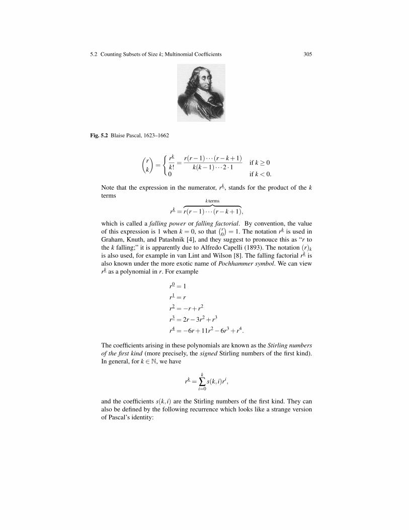
5.2 Counting Subsets of Size k; Multinomial Coefficients 305
Fig. 5.2 Blaise Pascal, 1623–1662
(rk
)=
rk
k!=
r(r−1) · · ·(r− k+1)k(k−1) · · ·2 ·1 if k ≥ 0
0 if k < 0.
Note that the expression in the numerator, rk, stands for the product of the kterms
rk =
k terms︷ ︸︸ ︷r(r−1) · · ·(r− k+1),
which is called a falling power or falling factorial. By convention, the valueof this expression is 1 when k = 0, so that
(r0
)= 1. The notation rk is used in
Graham, Knuth, and Patashnik [4], and they suggest to pronouce this as “r tothe k falling;” it is apparently due to Alfredo Capelli (1893). The notation (r)kis also used, for example in van Lint and Wilson [8]. The falling factorial rk isalso known under the more exotic name of Pochhammer symbol. We can viewrk as a polynomial in r. For example
r0 = 1
r1 = r
r2 =−r+ r2
r3 = 2r−3r2 + r3
r4 =−6r+11r2−6r3 + r4.
The coefficients arising in these polynomials are known as the Stirling numbersof the first kind (more precisely, the signed Stirling numbers of the first kind).In general, for k ∈ N, we have
rk =k
∑i=0
s(k, i)ri,
and the coefficients s(k, i) are the Stirling numbers of the first kind. They canalso be defined by the following recurrence which looks like a strange versionof Pascal’s identity:
306 5 Some Counting Problems; Binomial and Multinomial Coefficients
s(0,0) = 1s(n+1,k) = s(n,k−1)−ns(n,k), 1≤ k ≤ n+1,
with s(n,k) = 0 if n ≤ 0 or k ≤ 0 except for (n,k) = (0,0), or if k > n. Re-markably, from a combinatorial point of view, the positive integer (−1)k−is(k, i)counts certain types of permutations of k elements (those having i cycles). Bydefinition, rk = k!
(rk
), and in particular if r = n ∈ N, then
nk =n!
(n− k)!.
The expression(r
k
)can also be viewed as a polynomial of degree k in r. The
generalized binomial coefficients allow for a useful extension of the binomialformula (see next) to real exponents. However, beware that the symmetry iden-tity does not make sense if r is not an integer and that it is false if r a negativeinteger. In particular, the formula
(−1k
)=( −1−1−k
)is always false! Also, the for-
mula in Proposition 5.4 (in terms of the factorial function) only makes sense fornatural numbers.
We now prove the “binomial formula” (also called “binomial theorem”).
Proposition 5.5. (Binomial Formula) For all n ∈ N and for all reals a,b ∈ R, (ormore generally, any two commuting variables a,b, i.e., satisfying ab = ba), we havethe formula:
(a+b)n = an +
(n1
)an−1b+ · · ·+
(nk
)an−kbk + · · ·+
(n
n−1
)abn−1 +bn.
The above can be written concisely as
(a+b)n =n
∑k=0
(nk
)an−kbk.
Proof . We proceed by induction on n. For n = 0, we have (a+b)0 = 1 and the sumon the right hand side is also 1, inasmuch as
(00
)= 1.
Assume inductively that the formula holds for n. Because
(a+b)n+1 = (a+b)n(a+b),
using the induction hypothesis, we get
(a+b)n+1 = (a+b)n(a+b)
=
(n
∑k=0
(nk
)an−kbk
)(a+b)
=n
∑k=0
(nk
)an+1−kbk +
n
∑k=0
(nk
)an−kbk+1
5.2 Counting Subsets of Size k; Multinomial Coefficients 307
= an+1 +n
∑k=1
(nk
)an+1−kbk +
n−1
∑k=0
(nk
)an−kbk+1 +bn+1
= an+1 +n
∑k=1
(nk
)an+1−kbk +
n
∑k=1
(n
k−1
)an+1−kbk +bn+1
= an+1 +n
∑k=1
((nk
)+
(n
k−1
))an+1−kbk +bn+1
=n+1
∑k=0
(n+1
k
)an+1−kbk,
where we used Proposition 5.3 to go from the next to the last line to the last line.This establishes the induction step and thus, proves the binomial formula. ut
The binomial formula is a very effective tool to obtain short proofs of identitiesabout the binomial coefficients. For example, let us prove that(
n0
)+
(n1
)+ · · ·+
(n
n−1
)+
(nn
)=
n
∑k=0
(nk
)= 2n.
Simply let a = b = 1 in the binomial formula! On the left hand side, we have2n = (1+ 1)n, and on the right hand side, the desired sum. Of course, we can alsojustify the above formula using a combinatorial argument, by observing that we arecounting the numbers of all subsets of a set with n elements in two different ways:one way is to group all subsets of size k, for k = 0, . . . ,n, and the other way is toconsider the totally of all these subsets.
Remark: The binomial formula can be generalized to the case where the exponentr is a real number (even negative). This result is usually known as the binomialtheorem or Newton’s generalized binomial theorem. Formally, the binomial theoremstates that
(a+b)r =∞
∑k=0
(rk
)ar−kbk, r ∈ N or |b/a|< 1.
Observe that when r is not a natural number, the right-hand side is an infinite sumand the condition |b/a| < 1 ensures that the series converges. For example, whena = 1 and r = 1/2, if we rename b as x, we get
(1+ x)12 =
∞
∑k=0
( 12k
)xk
= 1+∞
∑k=1
1k!
12
(12−1)(
12−2)· · ·(
12− k+1
)xk
= 1+∞
∑k=1
(−1)k−1 1 ·3 ·5 · · ·(2k−3)2 ·4 ·6 · · ·2k
xk
308 5 Some Counting Problems; Binomial and Multinomial Coefficients
= 1+∞
∑k=1
(−1)k−1(2k)!(2k−1)(k!)222k xk
= 1+∞
∑k=1
(−1)k−1
22k(2k−1)
(2kk
)xk
= 1+∞
∑k=1
(−1)k−1
22k−11k
(2k−2k−1
)xk
which converges if |x|< 1. The first few terms of this series are
(1+ x)12 = 1+
12
x− 18
x2 +116
x3− 5128
x4 + · · · ,
For r =−1, we get the familiar geometric series
11+ x
= 1− x+ x2− x3 + · · ·+(−1)kxk + · · · ,
which converges if |x|< 1.We also stated earlier that the number of injections between a set with m elements
and a set with n elements, where m≤ n, is given by n!/(n−m)! and we now proveit.
Proposition 5.6. The number of injections between a set A with m elements and a setB with n elements, where m≤ n, is given by n!/(n−m)! = n(n−1) · · ·(n−m+1).
Proof . We proceed by induction on m ≤ n. If m = 0, then A = /0 and there is onlyone injection, namely the empty function from /0 to B. Because
n!(n−0)!
=n!n!
= 1,
the base case holds.Assume the induction hypothesis holds for m and consider a set A with m+ 1
elements, where m+1≤ n. Pick any element a ∈ A and let A′ = A−a, a set withm elements. Any injection f : A→ B assigns some element f (a) ∈ B to a and thenf A′ is an injection from A′ to B′ = B− f (a), a set with n−1 elements. By theinduction hypothesis, there are
(n−1)!(n−1−m)!
injections from A′ to B′. There are n ways of picking f (a) in B, therefore the numberof injections from A to B is
n(n−1)!
(n−1−m)!=
n!(n− (m+1))!
,
establishing the induction hypothesis. ut

5.2 Counting Subsets of Size k; Multinomial Coefficients 309
Observe that n!/(n−m)! = n(n−1) · · ·(n−m+1) = nm, a falling factorial.Counting the number of surjections between a set with n elements and a set with
p elements, where n≥ p, is harder. We state the following formula without giving aproof right now. Finding a proof of this formula is an interesting exercise. We givea quick proof using the principle of inclusion–exclusion in Section 5.4.
Proposition 5.7. The number of surjections Sn p between a set A with n elementsand a set B with p elements, where n≥ p, is given by
Sn p = pn−(
p1
)(p−1)n +
(p2
)(p−2)n + · · ·+(−1)p−1
(p
p−1
).
Remarks:
1. It can be shown that Sn p satisfies the following peculiar version of Pascal’srecurrence formula,
Sn p = p(Sn−1 p +Sn−1 p−1), p≥ 2,
and, of course, Sn1 = 1 and Sn p = 0 if p > n. Using this recurrence formula andthe fact that Snn = n!, simple expressions can be obtained for Sn+1n and Sn+2n.
2. The numbers Sn p are intimately related to the so-called Stirling numbers of thesecond kind, denoted
np
, S(n, p), or S(p)
n , which count the number of partitionsof a set of n elements into p nonempty pairwise disjoint blocks (see Section3.9). In fact,
Sn p = p!
np
.
The Stirling numbersn
p
satisfy a recurrence equation that is another variant
of Pascal’s recurrence formula:n1
= 1
nn
= 1
np
=
n−1p−1
+ p
n−1p
(1≤ p < n).
The Stirling numbers of the first kind and the Stirling numbers of the secondkind are very closely related. Indeed, they can be obtained from each other bymatrix inversion; see Problem 5.8.
3. The total numbers of partitions of a set with n≥ 1 elements is given by the Bellnumber,
bn =n
∑p=1
np
.
310 5 Some Counting Problems; Binomial and Multinomial Coefficients
There is a recurrence formula for the Bell numbers but it is complicated and notvery useful because the formula for bn+1 involves all the previous Bell numbers.
Fig. 5.3 Eric Temple Bell, 1883–1960 (left) and Donald Knuth, 1938– (right)
A good reference for all these special numbers is Graham, Knuth, and Patashnik[4], Chapter 6.
The binomial coefficients can be generalized as follows. For all n,m,k1, . . . ,km ∈N, with k1 + · · ·+ km = n and m≥ 2, we have the multinomial coefficient,(
nk1, . . . ,km
),
which counts the number of ways of splitting a set of n elements into an orderedsequence of m disjoint subsets, the ith subset having ki≥ 0 elements. Such sequencesof disjoint subsets whose union is 1, . . . ,n itself are sometimes called orderedpartitions.
Beware that some of the subsets in an ordered partition may be empty, so we feelthat the terminology “partition” is confusing because as we show in Section 3.9, thesubsets that form a partition are never empty. Note that when m = 2, the number ofways of splitting a set of n elements into two disjoint subsets where the first subsethas k1 elements and the second subset has k2 = n− k1 elements is precisely thenumber of subsets of size k1 of a set of n elements; that is,(
nk1,k2
)=
(nk1
).
An ordered partition is an ordered sequence
(S1, . . . ,Sm)
of m disjoint subsets Si ⊆ 1, . . . ,n, such that Si has ki ≥ 0 elements. We can thinkof the numbers 1,2, . . . ,m as the labels of boxes Si that split the set 1, . . . ,n intom disjoint parts, with ki elements in box Si.
Beware that defining an ordered partition as a set

5.2 Counting Subsets of Size k; Multinomial Coefficients 311
S1, . . . ,Sm
of m disjoint subsets Si ⊆ 1, . . . ,n, such that Si has ki ≥ 0 elements, is wrong!The problem with using a set of boxes is that that we do not keep track of the
assignment of objects to boxes. For example, for n = 5, m = 4, k1 = 2, and k2 =k3 = k4 = 1, the sequences of subsets (S1,S2,S3,S4) given by (1,2,3,4,5),(1,2,3,5,4), (1,2,5,3,4), (1,2,4,3,5), (1,2,4,5,3), (1,2,5,4,3) are all different. For example the ordered partitionobtained by placing 1,2 in box S1, 3 in box S2, 4 in box S3, and 5 in box S4, is notthe same as the ordered partition obtained by placing 1,2 in box S1, 3 in box S2, 5in box S3, and 4 in box S4. Not distinguishing among the order of S2,S3,S4, yields1,2,3,4,5, which does not capture the other 5 ordered partitions.
How do we construct ordered partitions? Consider the case n = 5, m = 3, k1 = 3,k2 = k3 = 1. Here, we have three boxes, S1,S2,S3, with |S1| = 3, |S2| = |S3| = 1.First, we can fill S3 with one of the five elements in 1, . . . ,5. For each of these, theremaining set is 1, . . . ,5−S3, and we can fill S2 with one of these four elements.There are three elements remaining in the set 1, . . . ,5−(S3∪S3), and box S1 mustbe filled with these elements. We obtain the following 20 ordered partitions:
(3,4,5,2,1), (2,4,5,3,1), (2,3,5,4,1), (2,3,4,5,1)(3,4,5,1,2), (1,4,5,3,2), (1,3,5,4,2), (1,3,4,5,2)(2,4,5,1,3), (1,4,5,2,3), (1,2,5,4,3), (1,2,4,5,3)(2,3,5,1,4), (1,3,5,2,4), (1,2,5,3,4), (1,2,3,5,4)(2,3,4,1,5), (1,3,4,2,5), (1,2,4,3,5), (1,2,3,4,5).
The principle of the proof of proposition 5.8 should now be clear.
Proposition 5.8. For all n,m,k1, . . . ,km ∈ N, with k1 + · · ·+ km = n and m ≥ 2, wehave (
nk1, . . . ,km
)=
n!k1! · · ·km!
.
Proof . There are( n
k1
)ways of forming a subset of k1 elements from the set of n
elements; there are(n−k1
k2
)ways of forming a subset of k2 elements from the remain-
ing n− k1 elements; there are(n−k1−k2
k3
)ways of forming a subset of k3 elements
from the remaining n− k1− k2 elements and so on; finally, there are(n−k1−···−km−2
km−1
)ways of forming a subset of km−1 elements from the remaining n− k1−·· ·− km−2elements and there remains a set of n− k1−·· ·− km−1 = km elements. This showsthat (
nk1, . . . ,km
)=
(nk1
)(n− k1
k2
)· · ·(
n− k1−·· ·− km−2
km−1
).
But then, using the fact that km = n− k1−·· ·− km−1, we get

312 5 Some Counting Problems; Binomial and Multinomial Coefficients(n
k1, . . . ,km
)=
n!k1!(n− k1)!
(n− k1)!k2!(n− k1− k2)!
· · · (n− k1−·· ·− km−2)!km−1!(n− k1−·· ·− km−1)!
=n!
k1! · · ·km!,
as claimed. ut
As in the binomial case, it is convenient to set(n
k1, . . . ,km
)= 0
if ki < 0 or ki > n, for any i, with 1≤ i≤ m.Proposition 5.8 show that the number of ordered partitions of n elements into m
boxes labeled 1,2, . . . ,m, with ki element in the ith box, does not depend on the orderin which the boxes are labeled. For every permutation π of 1, . . . ,m, the numberof ordered partitions of n elements into m boxes labeled π(1),π(2), . . . ,π(m), withkπ(i) element in the ith box, is also
( nk1,...,km
).
Another useful way to interpret the multinomial coefficients( n
k1,...,km
)is as the
number of strings of length n formed using an alphabet of m letters, say a1, . . . ,am,with ki occurrences of the letter ai, for i = 1, . . . ,m. For example, if n = 4, m = 2,k1 = 2 and k2 = 2, writing the alphabet as A,G (instead of a1,a2), we have thefollowing six strings:
AAGG, AGAG, GAAG, AGGA, GAGA, GGAA.
If n = 5, m = 3, k1 = 3, k2 = k3 = 1, if we let the alphabet be A,G,T, then weobtain the following 20 strings:
T GAAA, TAGAA, TAAGA, TAAAG
GTAAA, AT GAA, ATAGA, ATAAG
GATAA, AGTAA, AAT GA, AATAG
GAATA, AGATA, AAGTA, AAAT G
GAAAT, AGAAT, AAGAT, AAAGT.
Indeed, in order to form a string of length 5 with three A’s, one G and one T , firstwe place a T in one of 5 positions, and then we place a G in one of 4 positions; atthis stage, the three A’s occupy the remaining positions.
In general, a string of length n over an alphabet of m letters a1, . . . ,am, withki occurrences of ai, is formed by first assigning k1 occurrences of a1 to any of the( n
k1
)subsets S1 of positions in 1, . . . ,n, then assigning k2 occurrences of a2 to
any of the(n−k1
k2
)subsets S2 of remaing positions in 1, . . . ,n−S1, then assigning
k3 occurrences of a3 to any of the(n−k1−k2
k3
)subsets S3 of remaing positions in
1, . . . ,n− (S1∪S2), and so on. In the end, we get
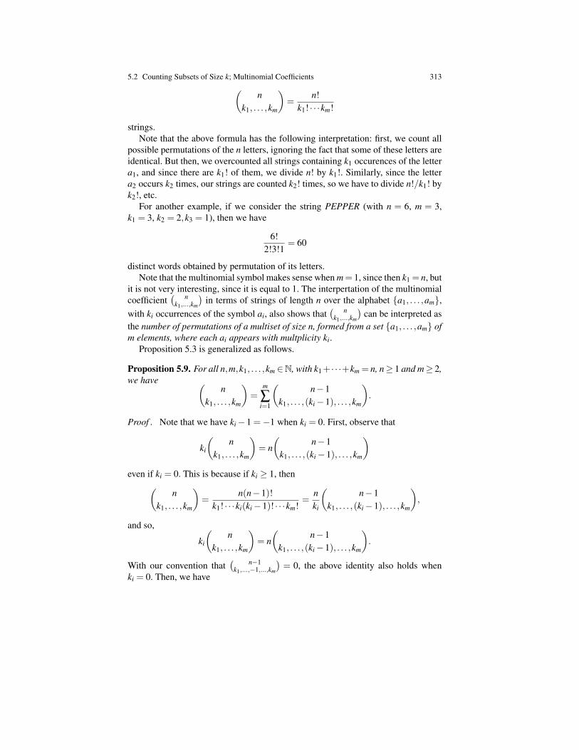
5.2 Counting Subsets of Size k; Multinomial Coefficients 313(n
k1, . . . ,km
)=
n!k1! · · ·km!
strings.Note that the above formula has the following interpretation: first, we count all
possible permutations of the n letters, ignoring the fact that some of these letters areidentical. But then, we overcounted all strings containing k1 occurences of the lettera1, and since there are k1! of them, we divide n! by k1!. Similarly, since the lettera2 occurs k2 times, our strings are counted k2! times, so we have to divide n!/k1! byk2!, etc.
For another example, if we consider the string PEPPER (with n = 6, m = 3,k1 = 3, k2 = 2,k3 = 1), then we have
6!2!3!1
= 60
distinct words obtained by permutation of its letters.Note that the multinomial symbol makes sense when m= 1, since then k1 = n, but
it is not very interesting, since it is equal to 1. The interpertation of the multinomialcoefficient
( nk1,...,km
)in terms of strings of length n over the alphabet a1, . . . ,am,
with ki occurrences of the symbol ai, also shows that( n
k1,...,km
)can be interpreted as
the number of permutations of a multiset of size n, formed from a set a1, . . . ,am ofm elements, where each ai appears with multplicity ki.
Proposition 5.3 is generalized as follows.
Proposition 5.9. For all n,m,k1, . . . ,km ∈N, with k1+ · · ·+km = n, n≥ 1 and m≥ 2,we have (
nk1, . . . ,km
)=
m
∑i=1
(n−1
k1, . . . ,(ki−1), . . . ,km
).
Proof . Note that we have ki−1 =−1 when ki = 0. First, observe that
ki
(n
k1, . . . ,km
)= n(
n−1k1, . . . ,(ki−1), . . . ,km
)even if ki = 0. This is because if ki ≥ 1, then(
nk1, . . . ,km
)=
n(n−1)!k1! · · ·ki(ki−1)! · · ·km!
=nki
(n−1
k1, . . . ,(ki−1), . . . ,km
),
and so,
ki
(n
k1, . . . ,km
)= n(
n−1k1, . . . ,(ki−1), . . . ,km
).
With our convention that( n−1
k1,...,−1,...,km
)= 0, the above identity also holds when
ki = 0. Then, we have
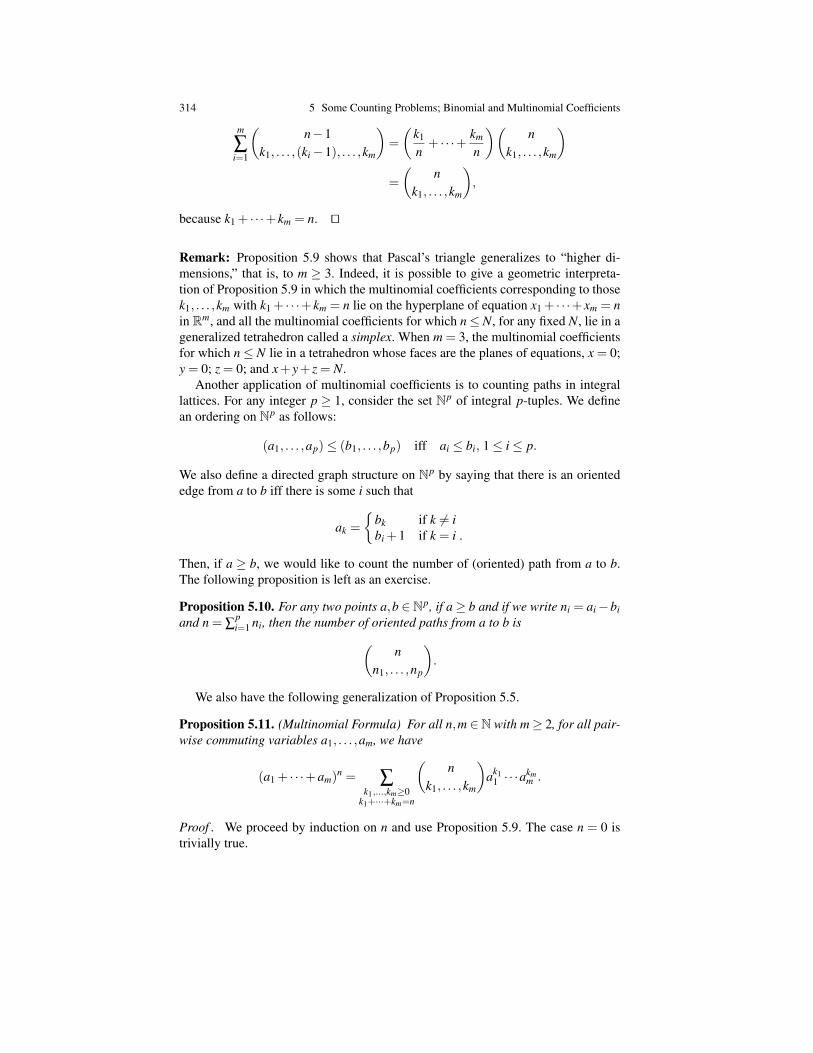
314 5 Some Counting Problems; Binomial and Multinomial Coefficients
m
∑i=1
(n−1
k1, . . . ,(ki−1), . . . ,km
)=
(k1
n+ · · ·+ km
n
)(n
k1, . . . ,km
)=
(n
k1, . . . ,km
),
because k1 + · · ·+ km = n. ut
Remark: Proposition 5.9 shows that Pascal’s triangle generalizes to “higher di-mensions,” that is, to m ≥ 3. Indeed, it is possible to give a geometric interpreta-tion of Proposition 5.9 in which the multinomial coefficients corresponding to thosek1, . . . ,km with k1 + · · ·+ km = n lie on the hyperplane of equation x1 + · · ·+ xm = nin Rm, and all the multinomial coefficients for which n≤ N, for any fixed N, lie in ageneralized tetrahedron called a simplex. When m = 3, the multinomial coefficientsfor which n≤ N lie in a tetrahedron whose faces are the planes of equations, x = 0;y = 0; z = 0; and x+ y+ z = N.
Another application of multinomial coefficients is to counting paths in integrallattices. For any integer p ≥ 1, consider the set Np of integral p-tuples. We definean ordering on Np as follows:
(a1, . . . ,ap)≤ (b1, . . . ,bp) iff ai ≤ bi, 1≤ i≤ p.
We also define a directed graph structure on Np by saying that there is an orientededge from a to b iff there is some i such that
ak =
bk if k 6= ibi +1 if k = i .
Then, if a ≥ b, we would like to count the number of (oriented) path from a to b.The following proposition is left as an exercise.
Proposition 5.10. For any two points a,b ∈Np, if a≥ b and if we write ni = ai−biand n = ∑
pi=1 ni, then the number of oriented paths from a to b is(
nn1, . . . ,np
).
We also have the following generalization of Proposition 5.5.
Proposition 5.11. (Multinomial Formula) For all n,m ∈N with m≥ 2, for all pair-wise commuting variables a1, . . . ,am, we have
(a1 + · · ·+am)n = ∑
k1,...,km≥0k1+···+km=n
(n
k1, . . . ,km
)ak1
1 · · ·akmm .
Proof . We proceed by induction on n and use Proposition 5.9. The case n = 0 istrivially true.

5.2 Counting Subsets of Size k; Multinomial Coefficients 315
Assume the induction hypothesis holds for n≥ 0, then we have
(a1 + · · ·+am)n+1 = (a1 + · · ·+am)
n(a1 + · · ·+am)
=
∑k1,...,km≥0
k1+···+km=n
(n
k1, . . . ,km
)ak1
1 · · ·akmm
(a1 + · · ·+am)
=m
∑i=1
∑k1,...,km≥0
k1+···+km=n
(n
k1, . . . ,ki, . . .km
)ak1
1 · · ·aki+1i · · ·akm
m
=m
∑i=1
∑k1,...,km≥0,ki≥1k1+···+km=n+1
(n
k1, . . . ,(ki−1), . . . ,km
)ak1
1 · · ·akii · · ·akm
m .
We seem to hit a snag, namely, that ki ≥ 1, but recall that(n
k1, . . . ,−1, . . . ,km
)= 0,
so we have
(a1 + · · ·+am)n+1 =
m
∑i=1
∑k1,...,km≥0,ki≥1k1+···+km=n+1
(n
k1, . . . ,(ki−1), . . . ,km
)ak1
1 · · ·akii · · ·akm
m
=m
∑i=1
∑k1,...,km≥0,
k1+···+km=n+1
(n
k1, . . . ,(ki−1), . . . ,km
)ak1
1 · · ·akii · · ·akm
m
= ∑k1,...,km≥0,
k1+···+km=n+1
(m
∑i=1
(n
k1, . . . ,(ki−1), . . . ,km
))ak1
1 · · ·akii · · ·akm
m
= ∑k1,...,km≥0,
k1+···+km=n+1
(n+1
k1, . . . ,ki, . . . ,km
)ak1
1 · · ·akii · · ·akm
m ,
where we used Proposition 5.9 to justify the last equation. Therefore, the inductionstep is proved and so is our proposition. ut
How many terms occur on the right-hand side of the multinomial formula? Aftera moment of reflection, we see that this is the number of finite multisets of sizen whose elements are drawn from a set of m elements, which is also equal to thenumber of m-tuples, k1, . . . ,km, with ki ∈ N and
k1 + · · ·+ km = n.
Thus, the problem is equivalent to placing n identical objects into m boxes, the ithbox consisting of ki ≥ 0 objects.
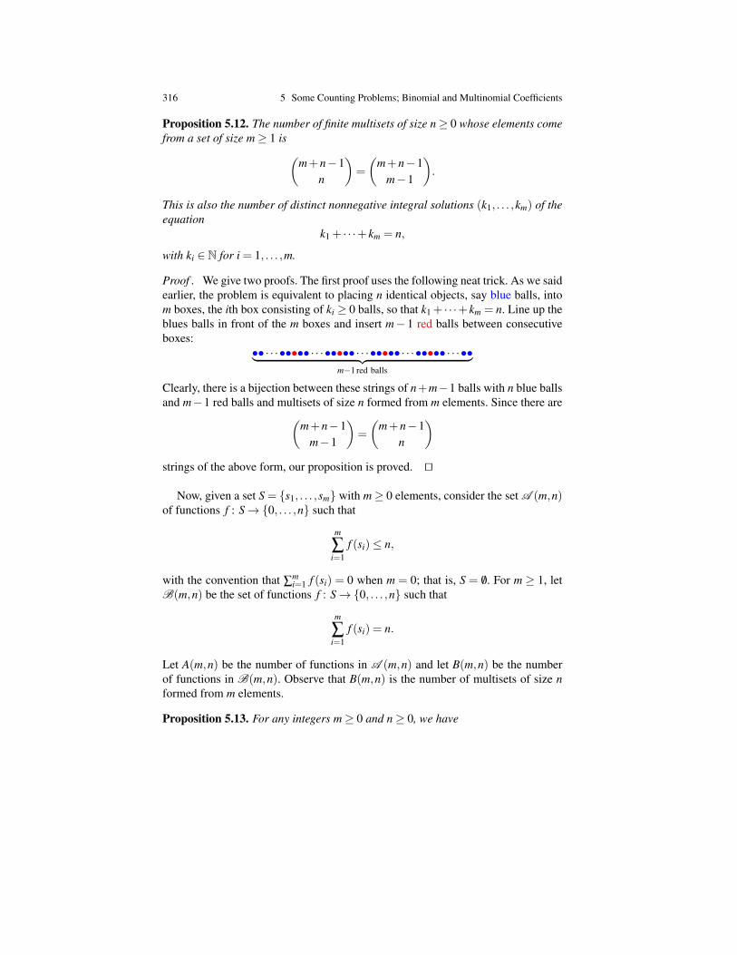
316 5 Some Counting Problems; Binomial and Multinomial Coefficients
Proposition 5.12. The number of finite multisets of size n≥ 0 whose elements comefrom a set of size m≥ 1 is (
m+n−1n
)=
(m+n−1
m−1
).
This is also the number of distinct nonnegative integral solutions (k1, . . . ,km) of theequation
k1 + · · ·+ km = n,
with ki ∈ N for i = 1, . . . ,m.
Proof . We give two proofs. The first proof uses the following neat trick. As we saidearlier, the problem is equivalent to placing n identical objects, say blue balls, intom boxes, the ith box consisting of ki ≥ 0 balls, so that k1 + · · ·+km = n. Line up theblues balls in front of the m boxes and insert m− 1 red balls between consecutiveboxes:
••· · ·•••••· · ·•••••· · ·•••••· · ·•••••· · ·••︸ ︷︷ ︸m−1 red balls
Clearly, there is a bijection between these strings of n+m−1 balls with n blue ballsand m−1 red balls and multisets of size n formed from m elements. Since there are(
m+n−1m−1
)=
(m+n−1
n
)strings of the above form, our proposition is proved. ut
Now, given a set S = s1, . . . ,sm with m≥ 0 elements, consider the set A (m,n)of functions f : S→0, . . . ,n such that
m
∑i=1
f (si)≤ n,
with the convention that ∑mi=1 f (si) = 0 when m = 0; that is, S = /0. For m ≥ 1, let
B(m,n) be the set of functions f : S→0, . . . ,n such that
m
∑i=1
f (si) = n.
Let A(m,n) be the number of functions in A (m,n) and let B(m,n) be the numberof functions in B(m,n). Observe that B(m,n) is the number of multisets of size nformed from m elements.
Proposition 5.13. For any integers m≥ 0 and n≥ 0, we have
5.2 Counting Subsets of Size k; Multinomial Coefficients 317
A(m,n) =(
m+nm
)B(m,n) =
(m+n−1
m−1
), m≥ 1.
Proof . First, we prove that
B(m,n) = A(m−1,n).
Let S′ = S−sm. Given any function f ∈B(m,n), we have ∑mi=1 f (si) = n, so the
restriction f ′ of f to S′ satisfies ∑m−1i=1 f (si) ≤ n; that is, f ′ ∈A (m−1,n). Further-
more,
f (sm) = n−m−1
∑i=1
f ′(si).
Conversely, given any function f ′ ∈A (m− 1,n), since ∑m−1i=1 f (si) ≤ n, we can
extend f ′ uniquely to a function f ∈B(m,n) by setting
f (sm) = n−m−1
∑i=1
f ′(si).
The map f 7→ f ′ is clearly a bijection between B(m,n) and A (m− 1,n), soB(m,n) = A(m−1,n), as claimed.
Next, we claim that
A(m,n) = A(m,n−1)+B(m,n).
This is because ∑mi=1 f (si) ≤ n iff either ∑
mi=1 f (si) = n or ∑
mi=1 f (si) ≤ n− 1. But
then, we get
A(m,n) = A(m,n−1)+B(m,n) = A(m,n−1)+A(m−1,n).
We finish the proof by induction on m+ n. For the base case m = n = 0, we knowthat A(0,0) = 1, and
(0+00
)=(0
0
)= 1, so this case holds.
For the induction step, m+n≥ 1, and by the induction hypothesis,
A(m,n−1) =(
m+n−1m
), A(m−1,n) =
(m+n−1
m−1
),
and using Pascal’s formula, we get
A(m,n) = A(m,n−1)+A(m−1,n)
=
(m+n−1
m−1
)+
(m+n−1
m
)=
(m+n
m
),

318 5 Some Counting Problems; Binomial and Multinomial Coefficients
establishing the induction step. ut
The proof of Proposition 5.13 yields another proof of Proposition 5.12 (but not asshort). Observe that given m variables X1, . . . ,Xm, Proposition 5.13 shows that thereare(m+n
m
)monomials
Xk11 · · ·Xkm
m
of total degree at most n (that is, k1 + · · ·+ km ≤ n), and(m+n−1
n
)=(m+n−1
m−1
)mono-
mials of total degree n (that is, k1 + · · ·+ km = n).
Proposition 5.14. The number of distinct positive integral solutions (k1, . . . ,km) ofthe equation
k1 + · · ·+ km = n
(with ki ∈ N and ki > 0, for i = 1, . . . ,m) is equal to(n−1m−1
).
Proof . We reduce this problem to the similar problem of counting the number ofdistinct nonnegative integral solutions of the equation
y1 + · · ·+ ym = p, yi ∈ N.
If we write yi = ki−1, then ki ∈ N−0 iff yi ∈ N, so our problem is equivalent todetermining the number of distinct nonnegative integral solutions of the equation
y1 + · · ·+ ym = n−m, yi ∈ N.
By Proposition 5.12, there are(m+n−m−1
m−1
)=
(n−1m−1
)such solutions. ut
The proof technique of Proposition 5.14 can be adapted to solve similar problemsinvolving constraints on the solutions (k1, . . . ,km) of the equation k1 + · · ·+ km = n.
5.3 Some Properties of the Binomial Coefficients
The binomial coefficients satisfy many remarkable identities.If one looks at the Pascal triangle, it is easy to figure out what are the sums of
the elements in any given row. It is also easy to figure out what are the sums ofn−m+1 consecutive elements in any given column (starting from the top and with0≤ m≤ n).
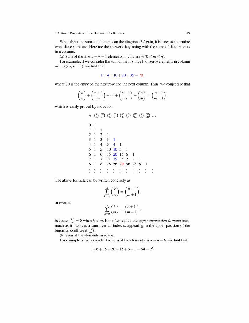
5.3 Some Properties of the Binomial Coefficients 319
What about the sums of elements on the diagonals? Again, it is easy to determinewhat these sums are. Here are the answers, beginning with the sums of the elementsin a column.
(a) Sum of the first n−m+1 elements in column m (0≤ m≤ n).For example, if we consider the sum of the first five (nonzero) elements in column
m = 3 (so, n = 7), we find that
1+4+10+20+35 = 70,
where 70 is the entry on the next row and the next column. Thus, we conjecture that(mm
)+
(m+1
m
)+ · · ·+
(n−1
m
)+
(nm
)=
(n+1m+1
),
which is easily proved by induction.
n(n
0
) (n1
) (n2
) (n3
) (n4
) (n5
) (n6
) (n7
) (n8
). . .
0 11 1 12 1 2 13 1 3 3 14 1 4 6 4 15 1 5 10 10 5 16 1 6 15 20 15 6 17 1 7 21 35 35 21 7 18 1 8 28 56 70 56 28 8 1...
......
......
......
......
......
The above formula can be written concisely as
n
∑k=m
(km
)=
(n+1m+1
),
or even asn
∑k=0
(km
)=
(n+1m+1
),
because(k
m
)= 0 when k < m. It is often called the upper summation formula inas-
much as it involves a sum over an index k, appearing in the upper position of thebinomial coefficient
(km
).
(b) Sum of the elements in row n.For example, if we consider the sum of the elements in row n = 6, we find that
1+6+15+20+15+6+1 = 64 = 26.

320 5 Some Counting Problems; Binomial and Multinomial Coefficients
n(n
0
) (n1
) (n2
) (n3
) (n4
) (n5
) (n6
) (n7
) (n8
). . .
0 11 1 12 1 2 13 1 3 3 14 1 4 6 4 15 1 5 10 10 5 16 1 6 15 20 15 6 17 1 7 21 35 35 21 7 18 1 8 28 56 70 56 28 8 1...
......
......
......
......
......
Thus, we conjecture that(n0
)+
(n1
)+ · · ·+
(n
n−1
)+
(nn
)= 2n.
This is easily proved by setting a = b = 1 in the binomial formula for (a+b)n.Unlike the columns for which there is a formula for the partial sums, there is no
closed-form formula for the partial sums of the rows. However, there is a closed-form formula for partial alternating sums of rows. Indeed, it is easily shown byinduction that
m
∑k=0
(−1)k(
nk
)= (−1)m
(n−1
m
),
if 0≤ m≤ n. For example,
1−7+21−35 =−20.
Also, for m = n, we getn
∑k=0
(−1)k(
nk
)= 0.
(c) Sum of the first n+1 elements on the descending diagonal starting from rowm.
For example, if we consider the sum of the first five elements starting from rowm = 3 (so, n = 4), we find that
1+4+10+20+35 = 70,
the elements on the next row below the last element, 35.
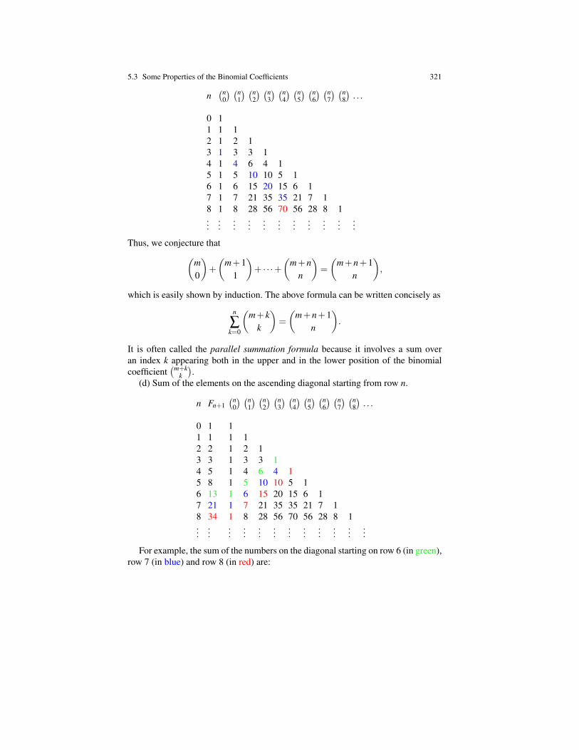
5.3 Some Properties of the Binomial Coefficients 321
n(n
0
) (n1
) (n2
) (n3
) (n4
) (n5
) (n6
) (n7
) (n8
). . .
0 11 1 12 1 2 13 1 3 3 14 1 4 6 4 15 1 5 10 10 5 16 1 6 15 20 15 6 17 1 7 21 35 35 21 7 18 1 8 28 56 70 56 28 8 1...
......
......
......
......
......
Thus, we conjecture that(m0
)+
(m+1
1
)+ · · ·+
(m+n
n
)=
(m+n+1
n
),
which is easily shown by induction. The above formula can be written concisely as
n
∑k=0
(m+ k
k
)=
(m+n+1
n
).
It is often called the parallel summation formula because it involves a sum overan index k appearing both in the upper and in the lower position of the binomialcoefficient
(m+kk
).
(d) Sum of the elements on the ascending diagonal starting from row n.
n Fn+1(n
0
) (n1
) (n2
) (n3
) (n4
) (n5
) (n6
) (n7
) (n8
). . .
0 1 11 1 1 12 2 1 2 13 3 1 3 3 14 5 1 4 6 4 15 8 1 5 10 10 5 16 13 1 6 15 20 15 6 17 21 1 7 21 35 35 21 7 18 34 1 8 28 56 70 56 28 8 1...
......
......
......
......
......
...
For example, the sum of the numbers on the diagonal starting on row 6 (in green),row 7 (in blue) and row 8 (in red) are:

322 5 Some Counting Problems; Binomial and Multinomial Coefficients
1+6+5+1 = 134+10+6+1 = 21
1+10+15+7+1 = 34.
We recognize the Fibonacci numbers F7,F8, and F9; what a nice surprise.Recall that F0 = 0, F1 = 1, and
Fn+2 = Fn+1 +Fn.
Thus, we conjecture that
Fn+1 =
(n0
)+
(n−1
1
)+
(n−2
2
)+ · · ·+
(0n
).
The above formula can indeed be proved by induction, but we have to distinguishthe two cases where n is even or odd.
We now list a few more formulae that are often used in the manipulations ofbinomial coefficients. They are among the “top ten binomial coefficient identities”listed in Graham, Knuth, and Patashnik [4]; see Chapter 5.
(e) The equation (ni
)(n− ik− i
)=
(ki
)(nk
),
holds for all n, i,k, with 0≤ i≤ k ≤ n.This is because we find that after a few calculations,(
ni
)(n− ik− i
)=
n!i!(k− i)!(n− k)!
=
(ki
)(nk
).
Observe that the expression in the middle is really the trinomial coefficient(n
ik− in− k
).
For this reason, the equation (e) is often called trinomial revision.For i = 1, we get
n(
n−1k−1
)= k(
nk
).
So, if k 6= 0, we get the equation(nk
)=
nk
(n−1k−1
), k 6= 0.
This equation is often called the absorption identity.(f) The equation (
m+ pn
)=
m
∑k=0
(mk
)(p
n− k
)
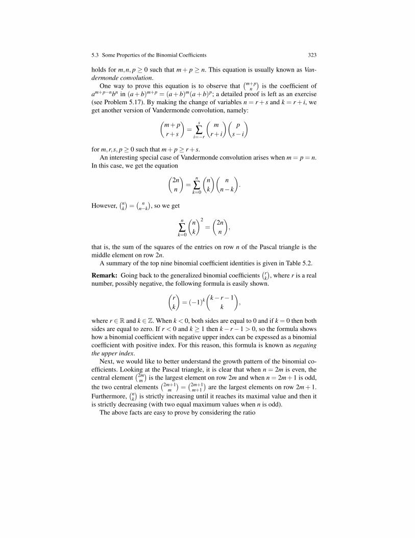
5.3 Some Properties of the Binomial Coefficients 323
holds for m,n, p ≥ 0 such that m+ p ≥ n. This equation is usually known as Van-dermonde convolution.
One way to prove this equation is to observe that(m+p
n
)is the coefficient of
am+p−nbn in (a+ b)m+p = (a+ b)m(a+ b)p; a detailed proof is left as an exercise(see Problem 5.17). By making the change of variables n = r+ s and k = r+ i, weget another version of Vandermonde convolution, namely:(
m+ pr+ s
)=
s
∑i=−r
(m
r+ i
)(p
s− i
)for m,r,s, p≥ 0 such that m+ p≥ r+ s.
An interesting special case of Vandermonde convolution arises when m = p = n.In this case, we get the equation(
2nn
)=
n
∑k=0
(nk
)(n
n− k
).
However,(n
k
)=( n
n−k
), so we get
n
∑k=0
(nk
)2
=
(2nn
),
that is, the sum of the squares of the entries on row n of the Pascal triangle is themiddle element on row 2n.
A summary of the top nine binomial coefficient identities is given in Table 5.2.
Remark: Going back to the generalized binomial coefficients(r
k
), where r is a real
number, possibly negative, the following formula is easily shown.(rk
)= (−1)k
(k− r−1
k
),
where r ∈R and k ∈ Z. When k < 0, both sides are equal to 0 and if k = 0 then bothsides are equal to zero. If r < 0 and k ≥ 1 then k− r−1 > 0, so the formula showshow a binomial coefficient with negative upper index can be expessed as a binomialcoefficient with positive index. For this reason, this formula is known as negatingthe upper index.
Next, we would like to better understand the growth pattern of the binomial co-efficients. Looking at the Pascal triangle, it is clear that when n = 2m is even, thecentral element
(2mm
)is the largest element on row 2m and when n = 2m+1 is odd,
the two central elements(2m+1
m
)=(2m+1
m+1
)are the largest elements on row 2m+ 1.
Furthermore,(n
k
)is strictly increasing until it reaches its maximal value and then it
is strictly decreasing (with two equal maximum values when n is odd).The above facts are easy to prove by considering the ratio
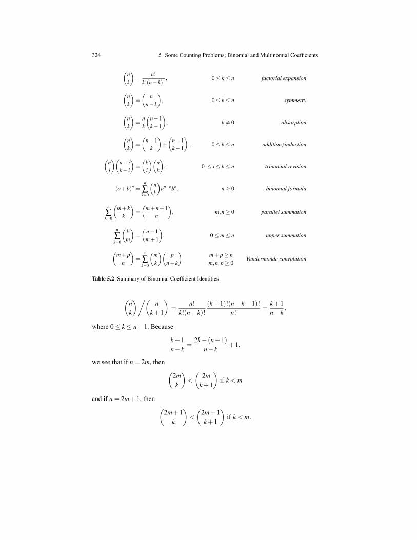
324 5 Some Counting Problems; Binomial and Multinomial Coefficients
(nk
)=
n!k!(n− k)!
, 0≤ k ≤ n factorial expansion
(nk
)=
(n
n− k
), 0≤ k ≤ n symmetry
(nk
)=
nk
(n−1k−1
), k 6= 0 absorption
(nk
)=
(n−1
k
)+
(n−1k−1
), 0≤ k ≤ n addition/induction
(ni
)(n− ik− i
)=
(ki
)(nk
), 0 ≤ i≤ k ≤ n trinomial revision
(a+b)n =n
∑k=0
(nk
)an−kbk, n≥ 0 binomial formula
n
∑k=0
(m+ k
k
)=
(m+n+1
n
), m,n≥ 0 parallel summation
n
∑k=0
(km
)=
(n+1m+1
), 0≤ m≤ n upper summation
(m+ p
n
)=
m
∑k=0
(mk
)(p
n− k
)m+ p≥ nm,n, p≥ 0
Vandermonde convolution
Table 5.2 Summary of Binomial Coefficient Identities
(nk
)/(n
k+1
)=
n!k!(n− k)!
(k+1)!(n− k−1)!n!
=k+1n− k
,
where 0≤ k ≤ n−1. Because
k+1n− k
=2k− (n−1)
n− k+1,
we see that if n = 2m, then (2mk
)<
(2m
k+1
)if k < m
and if n = 2m+1, then (2m+1
k
)<
(2m+1k+1
)if k < m.
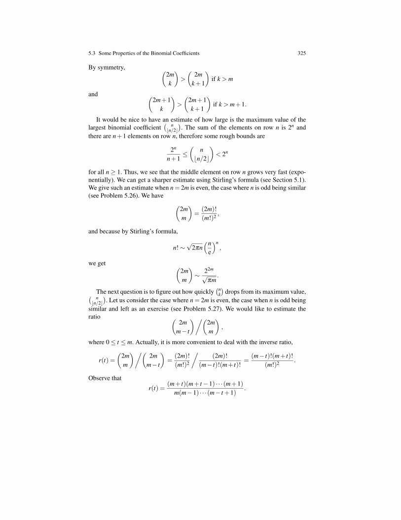
5.3 Some Properties of the Binomial Coefficients 325
By symmetry, (2mk
)>
(2m
k+1
)if k > m
and (2m+1
k
)>
(2m+1k+1
)if k > m+1.
It would be nice to have an estimate of how large is the maximum value of thelargest binomial coefficient
( nbn/2c
). The sum of the elements on row n is 2n and
there are n+1 elements on row n, therefore some rough bounds are
2n
n+1≤(
nbn/2c
)< 2n
for all n≥ 1. Thus, we see that the middle element on row n grows very fast (expo-nentially). We can get a sharper estimate using Stirling’s formula (see Section 5.1).We give such an estimate when n= 2m is even, the case where n is odd being similar(see Problem 5.26). We have (
2mm
)=
(2m)!(m!)2 ,
and because by Stirling’s formula,
n!∼√
2πn(n
e
)n,
we get (2mm
)∼ 22m√
πm.
The next question is to figure out how quickly(n
k
)drops from its maximum value,( n
bn/2c). Let us consider the case where n = 2m is even, the case when n is odd being
similar and left as an exercise (see Problem 5.27). We would like to estimate theratio (
2mm− t
)/(2mm
),
where 0≤ t ≤ m. Actually, it is more convenient to deal with the inverse ratio,
r(t) =(
2mm
)/(2m
m− t
)=
(2m)!(m!)2
/(2m)!
(m− t)!(m+ t)!=
(m− t)!(m+ t)!(m!)2 .
Observe that
r(t) =(m+ t)(m+ t−1) · · ·(m+1)
m(m−1) · · ·(m− t +1).
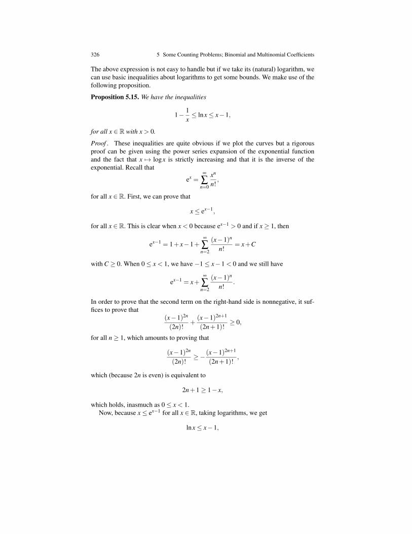
326 5 Some Counting Problems; Binomial and Multinomial Coefficients
The above expression is not easy to handle but if we take its (natural) logarithm, wecan use basic inequalities about logarithms to get some bounds. We make use of thefollowing proposition.
Proposition 5.15. We have the inequalities
1− 1x≤ lnx≤ x−1,
for all x ∈ R with x > 0.
Proof . These inequalities are quite obvious if we plot the curves but a rigorousproof can be given using the power series expansion of the exponential functionand the fact that x 7→ logx is strictly increasing and that it is the inverse of theexponential. Recall that
ex =∞
∑n=0
xn
n!,
for all x ∈ R. First, we can prove that
x≤ ex−1,
for all x ∈ R. This is clear when x < 0 because ex−1 > 0 and if x≥ 1, then
ex−1 = 1+ x−1+∞
∑n=2
(x−1)n
n!= x+C
with C ≥ 0. When 0≤ x < 1, we have −1≤ x−1 < 0 and we still have
ex−1 = x+∞
∑n=2
(x−1)n
n!.
In order to prove that the second term on the right-hand side is nonnegative, it suf-fices to prove that
(x−1)2n
(2n)!+
(x−1)2n+1
(2n+1)!≥ 0,
for all n≥ 1, which amounts to proving that
(x−1)2n
(2n)!≥− (x−1)2n+1
(2n+1)!,
which (because 2n is even) is equivalent to
2n+1≥ 1− x,
which holds, inasmuch as 0≤ x < 1.Now, because x≤ ex−1 for all x ∈ R, taking logarithms, we get
lnx≤ x−1,
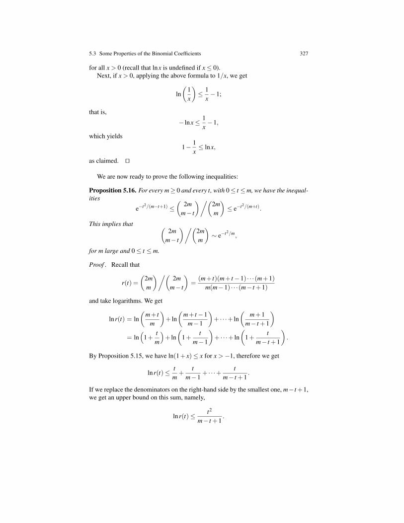
5.3 Some Properties of the Binomial Coefficients 327
for all x > 0 (recall that lnx is undefined if x≤ 0).Next, if x > 0, applying the above formula to 1/x, we get
ln(
1x
)≤ 1
x−1;
that is,
− lnx≤ 1x−1,
which yields
1− 1x≤ lnx,
as claimed. ut
We are now ready to prove the following inequalities:
Proposition 5.16. For every m≥ 0 and every t, with 0≤ t ≤m, we have the inequal-ities
e−t2/(m−t+1) ≤(
2mm− t
)/(2mm
)≤ e−t2/(m+t).
This implies that (2m
m− t
)/(2mm
)∼ e−t2/m,
for m large and 0≤ t ≤ m.
Proof . Recall that
r(t) =(
2mm
)/(2m
m− t
)=
(m+ t)(m+ t−1) · · ·(m+1)m(m−1) · · ·(m− t +1)
and take logarithms. We get
lnr(t) = ln(
m+ tm
)+ ln
(m+ t−1
m−1
)+ · · ·+ ln
(m+1
m− t +1
)= ln
(1+
tm
)+ ln
(1+
tm−1
)+ · · ·+ ln
(1+
tm− t +1
).
By Proposition 5.15, we have ln(1+ x)≤ x for x >−1, therefore we get
lnr(t)≤ tm+
tm−1
+ · · ·+ tm− t +1
.
If we replace the denominators on the right-hand side by the smallest one, m− t+1,we get an upper bound on this sum, namely,
lnr(t)≤ t2
m− t +1.
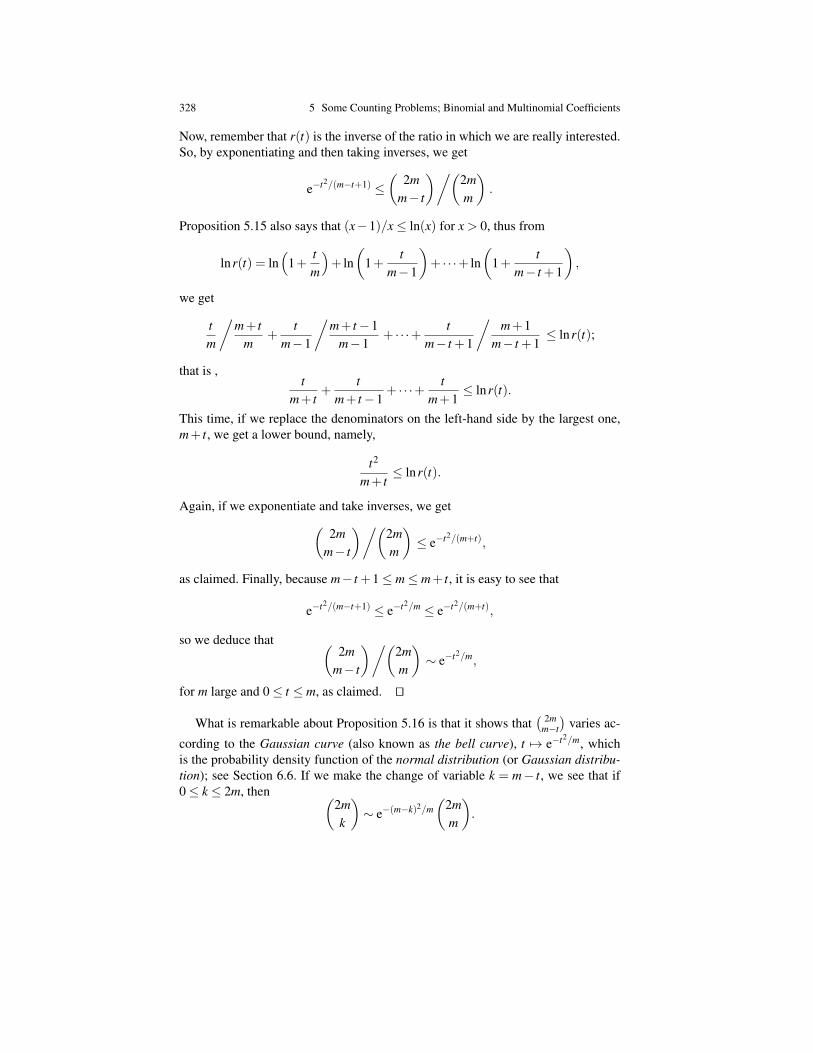
328 5 Some Counting Problems; Binomial and Multinomial Coefficients
Now, remember that r(t) is the inverse of the ratio in which we are really interested.So, by exponentiating and then taking inverses, we get
e−t2/(m−t+1) ≤(
2mm− t
)/(2mm
).
Proposition 5.15 also says that (x−1)/x≤ ln(x) for x > 0, thus from
lnr(t) = ln(
1+tm
)+ ln
(1+
tm−1
)+ · · ·+ ln
(1+
tm− t +1
),
we get
tm
/m+ t
m+
tm−1
/m+ t−1
m−1+ · · ·+ t
m− t +1
/m+1
m− t +1≤ lnr(t);
that is ,t
m+ t+
tm+ t−1
+ · · ·+ tm+1
≤ lnr(t).
This time, if we replace the denominators on the left-hand side by the largest one,m+ t, we get a lower bound, namely,
t2
m+ t≤ lnr(t).
Again, if we exponentiate and take inverses, we get(2m
m− t
)/(2mm
)≤ e−t2/(m+t),
as claimed. Finally, because m− t +1≤ m≤ m+ t, it is easy to see that
e−t2/(m−t+1) ≤ e−t2/m ≤ e−t2/(m+t),
so we deduce that (2m
m− t
)/(2mm
)∼ e−t2/m,
for m large and 0≤ t ≤ m, as claimed. ut
What is remarkable about Proposition 5.16 is that it shows that( 2m
m−t
)varies ac-
cording to the Gaussian curve (also known as the bell curve), t 7→ e−t2/m, whichis the probability density function of the normal distribution (or Gaussian distribu-tion); see Section 6.6. If we make the change of variable k = m− t, we see that if0≤ k ≤ 2m, then (
2mk
)∼ e−(m−k)2/m
(2mm
).

5.3 Some Properties of the Binomial Coefficients 329
If we plot this curve, we observe that it reaches its maximum for k = m and that itdecays very quickly as k varies away from m. It is an interesting exercise to plot abar chart of the binomial coefficients and the above curve together, say for m = 50.One will find that the bell curve is an excellent fit.
Given some number c > 1, it sometimes desirable to find for which values of tdoes the inequality (
2mm
)/(2m
m− t
)> c
hold. This question can be answered using Proposition 5.16.
Proposition 5.17. For every constant c > 1 and every natural number m≥ 0, if√m lnc+ lnc≤ t ≤ m, then (
2mm
)/(2m
m− t
)> c
and if 0≤ t ≤√
m lnc− lnc≤ m, then(2mm
)/(2m
m− t
)≤ c.
The proof uses the inequalities of Proposition 5.16 and is left as an exercise (seeProblem 5.28). As an example, if m = 1000 and c = 100, we have(
1000500
)/(1000
500− (500− k)
)> 100
or equivalently (1000
k
)/(1000500
)<
1100
when 500− k ≥√
500ln100+ ln100, that is, when
k ≤ 447.4.
It is also possible to give an upper on the partial sum(2m0
)+
(2m1
)+ · · ·+
(2m
k−1
),
with 0 ≤ k ≤ m in terms of the ratio c =(2m
k
)/(2mm
). The following proposition is
taken from Lovasz, Pelikan, and Vesztergombi [5].
Proposition 5.18. For any natural numbers m and k with 0≤ k ≤ m, if we letc =
(2mk
)/(2mm
), then we have
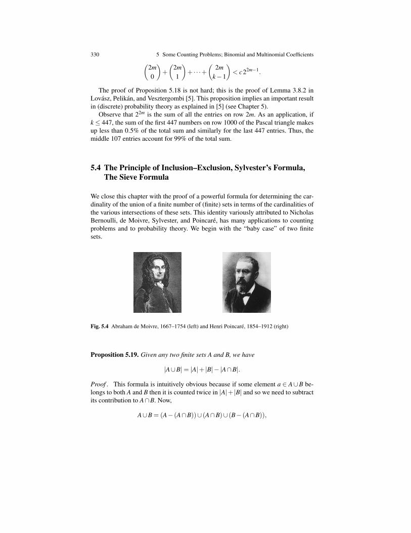
330 5 Some Counting Problems; Binomial and Multinomial Coefficients(2m0
)+
(2m1
)+ · · ·+
(2m
k−1
)< c22m−1.
The proof of Proposition 5.18 is not hard; this is the proof of Lemma 3.8.2 inLovasz, Pelikan, and Vesztergombi [5]. This proposition implies an important resultin (discrete) probability theory as explained in [5] (see Chapter 5).
Observe that 22m is the sum of all the entries on row 2m. As an application, ifk ≤ 447, the sum of the first 447 numbers on row 1000 of the Pascal triangle makesup less than 0.5% of the total sum and similarly for the last 447 entries. Thus, themiddle 107 entries account for 99% of the total sum.
5.4 The Principle of Inclusion–Exclusion, Sylvester’s Formula,The Sieve Formula
We close this chapter with the proof of a powerful formula for determining the car-dinality of the union of a finite number of (finite) sets in terms of the cardinalities ofthe various intersections of these sets. This identity variously attributed to NicholasBernoulli, de Moivre, Sylvester, and Poincare, has many applications to countingproblems and to probability theory. We begin with the “baby case” of two finitesets.
Fig. 5.4 Abraham de Moivre, 1667–1754 (left) and Henri Poincare, 1854–1912 (right)
Proposition 5.19. Given any two finite sets A and B, we have
|A∪B|= |A|+ |B|− |A∩B|.
Proof . This formula is intuitively obvious because if some element a ∈ A∪B be-longs to both A and B then it is counted twice in |A|+ |B| and so we need to subtractits contribution to A∩B. Now,
A∪B = (A− (A∩B))∪ (A∩B)∪ (B− (A∩B)),

5.4 The Principle of Inclusion–Exclusion 331
where the three sets on the right-hand side are pairwise disjoint. If we let a = |A|,b = |B|, and c = |A∩B|, then it is clear that
|A− (A∩B)| = a− c
|B− (A∩B)| = b− c,
so we get
|A∪B| = |A− (A∩B)|+ |A∩B|+ |B− (A∩B)|= a− c+ c+b− c = a+b− c
= |A|+ |B|− |A∩B|,
as desired. One can also give a proof by induction on n = |A∪B|. ut
We generalize the formula of Proposition 5.19 to any finite collection of finitesets, A1, . . . ,An. A moment of reflection shows that when n = 3, we have
|A∪B∪C|= |A|+ |B|+ |C|− |A∩B|− |A∩C|− |B∩C|+ |A∩B∩C|.
One of the obstacles in generalizing the above formula to n sets is purely notational.We need a way of denoting arbitrary intersections of sets belonging to a family ofsets indexed by 1, . . . ,n. We can do this by using indices ranging over subsetsof 1, . . . ,n, as opposed to indices ranging over integers. So, for example, for anynonempty subset I ⊆ 1, . . . ,n, the expression
⋂i∈I Ai denotes the intersection of
all the subsets whose index i belongs to I.
Theorem 5.1. (Principle of Inclusion–Exclusion) For any finite sequence A1, . . . ,An, of n≥ 2 subsets of a finite set X, we have∣∣∣∣∣ n⋃
k=1
Ak
∣∣∣∣∣= ∑I⊆1,...,n
I 6= /0
(−1)(|I|−1)
∣∣∣∣∣⋂i∈I
Ai
∣∣∣∣∣ .Proof . We proceed by induction on n≥ 2. The base case, n = 2, is exactly Propo-sition 5.19. Let us now consider the induction step. We can write
n+1⋃k=1
Ak =
(n⋃
k=1
Ak
)∪An+1
and so, by Proposition 5.19, we have∣∣∣∣∣n+1⋃k=1
Ak
∣∣∣∣∣ =∣∣∣∣∣(
n⋃k=1
Ak
)∪An+1
∣∣∣∣∣=
∣∣∣∣∣ n⋃k=1
Ak
∣∣∣∣∣+ |An+1|−∣∣∣∣∣(
n⋃k=1
Ak
)∩An+1
∣∣∣∣∣ .
332 5 Some Counting Problems; Binomial and Multinomial Coefficients
We can apply the induction hypothesis to the first term and we get∣∣∣∣∣ n⋃k=1
Ak
∣∣∣∣∣= ∑J⊆1,...,n
J 6= /0
(−1)(|J|−1)
∣∣∣∣∣⋂j∈J
A j
∣∣∣∣∣ .Using distributivity of intersection over union, we have(
n⋃k=1
Ak
)∩An+1=
n⋃k=1
(Ak ∩An+1).
Again, we can apply the induction hypothesis and obtain
−∣∣∣∣∣ n⋃k=1
(Ak ∩An+1)
∣∣∣∣∣ = − ∑J⊆1,...,n
J 6= /0
(−1)(|J|−1)
∣∣∣∣∣⋂j∈J
(A j ∩An+1)
∣∣∣∣∣= ∑
J⊆1,...,nJ 6= /0
(−1)|J|
∣∣∣∣∣∣ ⋂j∈J∪n+1
A j
∣∣∣∣∣∣= ∑
J⊆1,...,nJ 6= /0
(−1)(|J∪n+1|−1)
∣∣∣∣∣∣ ⋂j∈J∪n+1
A j
∣∣∣∣∣∣ .Putting all this together, we get∣∣∣∣∣n+1⋃
k=1
Ak
∣∣∣∣∣ = ∑J⊆1,...,n
J 6= /0
(−1)(|J|−1)
∣∣∣∣∣⋂j∈J
A j
∣∣∣∣∣+ |An+1|
+ ∑J⊆1,...,n
J 6= /0
(−1)(|J∪n+1|−1)
∣∣∣∣∣∣ ⋂j∈J∪n+1
A j
∣∣∣∣∣∣= ∑
J⊆1,...,n+1J 6= /0,n+1/∈J
(−1)(|J|−1)
∣∣∣∣∣⋂j∈J
A j
∣∣∣∣∣+ ∑J⊆1,...,n+1
n+1∈J
(−1)(|J|−1)
∣∣∣∣∣⋂j∈J
A j
∣∣∣∣∣= ∑
I⊆1,...,n+1I 6= /0
(−1)(|I|−1)
∣∣∣∣∣⋂i∈I
Ai
∣∣∣∣∣ ,establishing the induction hypothesis and finishing the proof. ut

5.4 The Principle of Inclusion–Exclusion 333
As an application of the inclusion–exclusion principle, let us prove the formulafor counting the number of surjections from 1, . . . ,n to 1, . . . , p, with p ≤ n,given in Proposition 5.7.
Recall that the total number of functions from 1, . . . ,n to 1, . . . , p is pn. Thetrick is to count the number of functions that are not surjective. Any such functionhas the property that its image misses one element from 1, . . . , p. So, if we let
Ai = f : 1, . . . ,n→ 1, . . . , p | i /∈ Im( f ),
we need to count |A1 ∪ ·· · ∪Ap|. But, we can easily do this using the inclusion–exclusion principle. Indeed, for any nonempty subset I of 1, . . . , p, with |I| = k,the functions in
⋂i∈I Ai are exactly the functions whose range misses I. But, these
are exactly the functions from 1, . . . ,n to 1, . . . , p−I and there are (p−k)n suchfunctions. Thus, ∣∣∣∣∣⋂
i∈I
Ai
∣∣∣∣∣= (p− k)n.
As there are(p
k
)subsets I ⊆ 1, . . . , p with |I| = k, the contribution of all k-fold
intersections to the inclusion–exclusion principle is(pk
)(p− k)n.
Note that A1 ∩ ·· · ∩Ap = /0, because functions have a nonempty image. Therefore,the inclusion–exclusion principle yields
|A1∪·· ·∪Ap|=p−1
∑k=1
(−1)k−1(
pk
)(p− k)n,
and so, the number of surjections Sn p is
Sn p = pn−|A1∪·· ·∪Ap|= pn−p−1
∑k=1
(−1)k−1(
pk
)(p− k)n
=p
∑k=0
(−1)k(
pk
)(p− k)n
= pn−(
p1
)(p−1)n +
(p2
)(p−2)n + · · ·+(−1)p−1
(p
p−1
),
which is indeed the formula of Proposition 5.7.Another amusing application of the inclusion–exclusion principle is the formula
giving the number pn of permutations of 1, . . . ,n that leave no element fixed (i.e.,f (i) 6= i, for all i ∈ 1, . . . ,n). Such permutations are often called derangements.We get
334 5 Some Counting Problems; Binomial and Multinomial Coefficients
pn = n!−(
n1
)(n−1)!+ · · ·+(−1)k
(nk
)(n− k)!+ · · ·+(−1)n
(nn
)= n!
(1− 1
1!+
12!
+ · · ·+ (−1)k
k!+ · · ·+ (−1)n
n!
).
Remark: We know (using the series expansion for ex in which we set x =−1) that
1e= 1− 1
1!+
12!
+ · · ·+ (−1)k
k!+ · · · .
Consequently, the factor of n! in the above formula for pn is the sum of the firstn+1 terms of 1/e and so,
limn→∞
pn
n!=
1e.
It turns out that the series for 1/e converges very rapidly, so pn ≈ n!/e. The ratiopn/n! has an interesting interpretation in terms of probabilities. Assume n personsgo to a restaurant (or to the theatre, etc.) and that they all check their coats. Unfor-tunately, the clerk loses all the coat tags. Then pn/n! is the probability that nobodywill get her or his own coat back. As we just explained, this probability is roughly1/e≈ 1/3, a surprisingly large number.
We can also count the number pn,r of permutations that leave r elements fixed;that is, f (i) = i for r elments i ∈ 1, . . . ,n, with 0≤ r ≤ n. We can pick
(nr
)subsets
of r elements that remain fixed, and the remaining n− r elements must all move, sowe have
pn,r =
(nr
)pn−r,
with p0 = 1. Thus, we have
pn,r =n−r
∑k=0
(−1)k(
nr
)(n− r
k
)(n− r− k)!
=n!r!
(n−r
∑k=0
(−1)k
k!
).
As a consequence,
limn→∞
pn,r
n!=
1r!e
.
The inclusion–exclusion principle can be easily generalized in a useful way asfollows. Given a finite set X , let m be any given function m : X → R+ and for anynonempty subset A⊆ X , set
m(A) = ∑a∈A
m(a),
5.4 The Principle of Inclusion–Exclusion 335
with the convention that m( /0) = 0 (recall that R+ = x ∈ R | x ≥ 0). For any x ∈X , the number m(x) is called the weight (or measure) of x and the quantity m(A)is often called the measure of the set A. For example, if m(x) = 1 for all x ∈ A,then m(A) = |A|, the cardinality of A, which is the special case that we have beenconsidering. For any two subsets A,B⊆ X , it is obvious that
m(A∪B) = m(A)+m(B)−m(A∩B)
m(X−A) = m(X)−m(A)
m(A∪B) = m(A∩B)
m(A∩B) = m(A∪B),
where A = X−A. Then, we have the following version of Theorem 5.1.
Theorem 5.2. (Principle of Inclusion–Exclusion, Version 2) Given any measurefunction m : X → R+, for any finite sequence A1, . . . ,An, of n ≥ 2 subsets of a fi-nite set X, we have
m
(n⋃
k=1
Ak
)= ∑
I⊆1,...,nI 6= /0
(−1)(|I|−1) m
(⋂i∈I
Ai
).
Proof . The proof is obtained from the proof of Theorem 5.1 by changing every-where any expression of the form |B| to m(B). ut
A useful corollary of Theorem 5.2 often known as Sylvester’s formula is thefollowing.
Fig. 5.5 James Joseph Sylvester, 1814–1897
Theorem 5.3. (Sylvester’s Formula) Given any measure m : X → R+, for any finitesequence A1, . . . ,An of n ≥ 2 subsets of a finite set X, the measure of the set ofelements of X that do not belong to any of the sets Ai is given by
m
(n⋂
k=1
Ak
)= m(X)+ ∑
I⊆1,...,nI 6= /0
(−1)|I|m
(⋂i∈I
Ai
).

336 5 Some Counting Problems; Binomial and Multinomial Coefficients
Proof . Observe thatn⋂
k=1
Ak = X−n⋃
k=1
Ak.
Consequently, using Theorem 5.2, we get
m
(n⋂
k=1
Ak
)= m
(X−
n⋃k=1
Ak
)
= m(X)−m
(n⋃
k=1
Ak
)
= m(X)− ∑I⊆1,...,n
I 6= /0
(−1)(|I|−1) m
(⋂i∈I
Ai
)
= m(X)+ ∑I⊆1,...,n
I 6= /0
(−1)|I|m
(⋂i∈I
Ai
),
establishing Sylvester’s formula. ut
Note that if we use the convention that when the index set I is empty then⋂i∈ /0
Ai = X ,
hence the term m(X) can be included in the above sum by removing the conditionthat I 6= /0 and this version of Sylvester’s formula is written:
m
(n⋂
k=1
Ak
)= ∑
I⊆1,...,n(−1)|I|m
(⋂i∈I
Ai
).
Sometimes, it is also convenient to regroup terms involving subsets I having thesame cardinality, and another way to state Sylvester’s formula is as follows.
m
(n⋂
k=1
Ak
)=
n
∑k=0
(−1)k∑
I⊆1,...,n|I|=k
m
(⋂i∈I
Ai
). (Sylvester’s Formula)
Sylvester’s formula can be used to give a quick proof for the formula for theEuler φ -function (or totient), which is defined as follows. For every positive integern, define φ(n) as the number of integers m ∈ 1, . . . ,n, such that m is relativelyprime to n (gcd(m,n) = 1). Observe that φ(1) = 1. Then, for any integer n ≥ 2, ifthe prime factorization of n is
n = pk11 · · · pkr
r ,
5.4 The Principle of Inclusion–Exclusion 337
where p1 < · · ·< pr are primes and ki ≥ 1, we have
φ(n) = n−r
∑i=1
npi
+r
∑1≤i< j≤r
npi p j−·· ·= n
r
∏i=1
(1− 1
pi
).
In order to obtain the above formula, let X = 1,2, . . . ,n, for each i with 1 ≤i ≤ r, set Ai to be the set of positive integers not divisible by pi, and for any i, letm(i) = 1.
As another application of Sylvester’s formula, let us prove the formula
n
∑i=0
(−1)i(
ni
)(m+n− i
k− i
)=
(mk
)if k ≤ m
0 if k > m.
To obtain a combinatorial proof of the above formula, let Y = y1, . . . ,yn be aset of n blue balls, and let Z = z1, . . . ,zm be a set of m red balls.
How many subsets of Y ∪Z of size k can we form consisting of red balls only?Clearly, the expression on the right hand side is the answer. We can also useSylvester’s formula to obtain the left hand side. Indeed, let X = Y ∪ Z, set Ai tobe the collection of all k-subsets of X containing yi, and let m(yi) = m(z j) = 1. Weleave it as an exercise to show that Sylvester’s formula yields the left hand side.
Finally, Sylvester’s formula can be generalized to a formula usually known as the“sieve formula.”
Theorem 5.4. (Sieve Formula) Given any measure m : X → R+ for any finite se-quence A1, . . . ,An of n≥ 2 subsets of a finite set X, the measure of the set of elementsof X that belong to exactly p of the sets Ai (0≤ p≤ n) is given by
T pn =
n
∑k=p
(−1)k−p(
kp
)∑
I⊆1,...,n|I|=k
m
(⋂i∈I
Ai
).
Proof . Observe that the set of elements of X that belong to exactly p of the sets Ai(with 0≤ p≤ n) is given by the expression
⋃I⊆1,...,n|I|=p
⋂i∈I
Ai∩⋂j/∈I
A j
.
For any subset I ⊆ 1, . . . ,n, if we apply Sylvester’s formula to X =⋂
i∈I Ai and tothe subsets A j ∩
⋂i∈I Ai for which j 6∈ I (i.e., j ∈ 1, . . . ,n− I), we get
m
⋂i∈I
Ai∩⋂j/∈I
A j
= ∑J⊆1,...,n
I⊆J
(−1)|J|−|I|m
(⋂j∈J
A j
).
Hence,

338 5 Some Counting Problems; Binomial and Multinomial Coefficients
T pn = ∑
I⊆1,...,n|I|=p
m
⋂i∈I
Ai∩⋂j/∈I
A j
= ∑
I⊆1,...,n|I|=p
∑J⊆1,...,n
I⊆J
(−1)|J|−|I|m
(⋂j∈J
A j
)
= ∑J⊆1,...,n|J|≥p
∑I⊆J|I|=p
(−1)|J|−|I|m
(⋂j∈J
A j
)
=n
∑k=p
(−1)k−p(
kp
)∑
J⊆1,...,n|J|=k
m
(⋂j∈J
A j
),
establishing the sieve formula. ut
Observe that Sylvester’s formula is the special case of the sieve formula for whichp = 0. The inclusion–exclusion principle (and its relatives) plays an important rolein combinatorics and probability theory as the reader may verify by consulting anytext on combinatorics.
5.5 Mobius Inversion Formula
There are situations, for example in the theory of error-correcting codes, where thefollowing situation arises: we have two functions f ,g : N+→R defined on the pos-itive natural numbers, and f and g are related by the equation
g(n) = ∑d|n
f (d), n ∈ N+,
where d | n means that d divides n (that is, n = kd, for some k ∈N). Then, there is afunction µ , the Mobius function, such that f is given in terms of g by the equation
f (n) = ∑d|n
µ(d)g(
nd
), n ∈ N+,
Such a formula is known as Mobius inversion.Roughly speaking, the Mobius function tests whether a positive integer is square-
free. A positive integer n is squarefree if it is not divisible by a square d2, with d ∈N,and d > 1. For example, n = 18 is not squarefree since it is divisible by 9 = 32. Onthe other hand, 15 = 3 ·5 is squarefree. If n≥ 2 is a positive integer and if
n = pk11 · · · pkr
r
5.5 Mobius Inversion Formula 339
is its prime factorization, where p1 < · · · < pr are primes and ki ≥ 1, then n issquarefree iff k1 = · · · = kr = 1. The Mobius function is the function µ : N+ →−1,0,1 defined as follows:
µ(n) =
1 if n = 1(−1)r if k1 = · · ·= kr = 1 in the prime factorization of n0 if n is not squarefree.
A crucial property of the function µ is stated in the following lemma, whose proofuses the formula for the alternating sum of the binomial coefficients that we obtainedin Section 5.3 (b).
Proposition 5.20. For every integer n ∈ N+, we have
∑d|n
µ(d) =
1 if n = 10 if n≥ 2.
Proof . The case where n= 1 is clear. Otherwise, if we write the prime factorizationof n as
n = pk11 · · · pkr
r ,
then by definition of µ , only the squarefree divisors contribute to the sum ∑d|n µ(d),and these correspond to the subsets of p1, . . . , pr (where /0 yields 1). Since thereare(r
i
)subsets I of size i, and since for each I,
µ
(∏I∈I
pi
)= (−1)i,
we get
∑d|n
µ(d) =r
∑i=0
(ri
)(−1)i.
However, ∑ri=0(r
i
)(−1)i = (1−1)r = 0, which concludes the proof. ut
Remark: Note that the Euler φ -function is also given by
φ(n) = ∑d|n
µ(d)nd.
Here is the famous Mobius inversion formula.
Theorem 5.5. (Mobius inversion formula) Let f ,g : N+→ R be any two functionsdefined on the positive natural numbers, and assume that f and g are related by theequation
g(n) = ∑d|n
f (d), n ∈ N+.
Then, f is given in terms of g by the equation

340 5 Some Counting Problems; Binomial and Multinomial Coefficients
f (n) = ∑d|n
µ(d)g(
nd
), n ∈ N+.
Proof . The proof consists in pushing and interchanging summations around, and itis not very illuminating. For any divisor d of n, the quotient n/d is also a divisor ofn, and conversely, so
∑d|n
µ(d)g(
nd
)= ∑
d|nµ
(nd
)g(d)
= ∑d|n
µ
(nd
)∑d′|d
f (d′).
Now, if d | n, then n = dd1 and if d′ | d, then d = d′d2, so n = d′d1d2. A moment ofreflexion(!) shows that
∑d|n
µ
(nd
)∑d′|d
f (d′) = ∑d′|n
f (d′) ∑m|(n/d′)
µ(m)
= f (n),
since by Proposition 5.20, we have
∑m|(n/d′)
µ(m) = 0,
unless d′ = n, in which case the sum has value 1. ut
Remark: A beautiful application of the Mobius inversion formula is the fact thatfor every finite field Fq of order q, for every integer n≥ 1, there is some irreduciblepolynomial of degee n with coefficients in Fq. This is a crucial fact in the theoryof error-correcting codes. In fact, if I (n,q) is the number of monic irreduciblepolynomials of degree n over Fq, then the following recurrence equation holds (seeCameron [2], Section 4.7 ):
qn = ∑d|n
dI (d,q).
By the Mobius inversion formula,
I (n,q) =1n ∑
d|nµ(d)q
nd .
For n = 1,2,3,4, we have
5.6 Summary 341
I (1,q) = q
I (2,q) =q(q−1)
2
I (3,q) =q(q−1)(q+1)
3
I (4,q) =q2(q−1)(q+1)
4.
Now, it is not hard to see that∣∣∣∣∣ ∑d|n,d 6=1
µ(d)qnd
∣∣∣∣∣≤ ∑d|n,d 6=1
qnd < qn,
which shows that I (n,q)> 0.Other interesting applications of the Mobius inversion formula are given in Gra-
ham, Knuth, and Patashnik [4] (Section 4.9). Mobius functions and the Mobiusinversion formula can be generalized to the more general setting of locally finiteposets; see Berge [1] and Stanley [7].
A classical reference on combinatorics is Berge [1]; a more recent one isCameron [2]; more advanced references are van Lint and Wilson [8] and Stanley[7]. Another great (but deceptively tough) reference covering discrete mathematicsand including a lot of combinatorics is Graham, Knuth, and Patashnik [4]. Conwayand Guy [3] is another beautiful book that presents many fascinating and intriguinggeometric and combinatorial properties of numbers in a very untertaining manner.For readers interested in geometry with a combinatriol flavor, Matousek [6] is adelightful (but more advanced) reference.
We are now ready to study special kinds of relations: partial orders and equiva-lence relations.
5.6 Summary
This chapter provided a very brief and elementary introduction to combinatorics.To be more precise, we considered various counting problems, such as countingthe number of permutations of a finite set, the number of functions from one set toanother, the number of injections from one set to another, the number of surjectionsfrom one set to another, the number of subsets of size k in a finite set of size n and thenumber of partitions of a set of size n into p blocks. This led us to the binomial (andthe multinomial) coefficients and various properties of these very special numbers.We also presented various formulae for determining the size of the union of a finitecollection of sets in terms of various intersections of these sets. We discussed theprinciple of inclusion–exclusion (PIE), Sylvester’s formula, and the sieve formula.
• We review the notion of a permutation and the factorial function (n 7→ n!).
342 5 Some Counting Problems; Binomial and Multinomial Coefficients
• We show that a set of size n has n! permutations.• We show that if A has m elements and B has n elements, then BA (the set of
functions from A to B) has nm elements.• We state Stirling’s formula, as an estimation of the factorial function.• We defined the “big oh” notation, the “big Ω” notation, the “big Θ” notation,
and the “little oh” notation.• We give recurrence relations for computing the number of subsets of size k
of a set of size n (the “Pascal recurrence relations”); these are the binomialcoefficients
(nk
).
• We give an explicit formula for(n
k
)and we prove the binomial formula (ex-
pressing (a+b)n in terms of the monomials an−kbk).• We define the falling factorial and introduce the Stirling numbers of the first
kind, s(n,k).• We give a formula for the number of injections from a finite set into another
finite set.• We state a formula for the number of surjections Sn p from a finite set of n
elements onto another finite set of p elements.• We relate the Sn p to the Stirling numbers of the second kind
np
that count the
number of partitions of a set of n elements into p disjoint blocks.• We define the bell numbers, which count the number of partitions of a finite set.• We define the multinomial coefficients
( nk1,...,km
)and give an explicit formula for
these numbers.• We prove the multinomial formula (expressing (a1 + · · ·+am)
n).• We count the number of multisets with n elements formed from a set of m
elements.• We prove some useful identities about the binomial coefficients summarized in
Table 5.2.• We estimate the value of the central (and largest) binomial coefficient
(2mm
)on
row 2m.• We give bounds for the ratio
( 2mm−t
)/(2mm
)and show that it is approximately
e−t2/m.• We prove the formula for the principle of inclusion–exclusion.• We apply this formula to derive a formula for Sn p.• We define derangements as permutations that leave no element fixed and give a
formula for counting them.• We generalize slightly the inclusion–exclusion principle by allowing finite sets
with weights (defining a measure on the set).• We prove Sylvester’s formula.• We prove the sieve formula.• We define the Mobius function and prove the Mobius inversion formula.
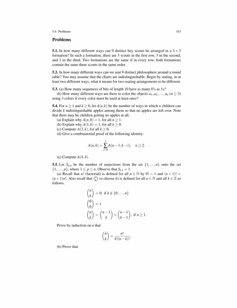
5.6 Problems 343
Problems
5.1. In how many different ways can 9 distinct boy scouts be arranged in a 3× 3formation? In such a formation, there are 3 scouts in the first row, 3 in the second,and 3 in the third. Two formations are the same if in every row, both formationscontain the same three scouts in the same order.
5.2. In how many different ways can we seat 9 distinct philosophers around a roundtable? You may assume that the chairs are indistinguishable. Begin by stating, in atleast two different ways, what it means for two seating arrangements to be different.
5.3. (a) How many sequences of bits of length 10 have as many 0’s as 1s?(b) How many different ways are there to color the objects a1,a2, . . . ,an (n≥ 3)
using 3 colors if every color must be used at least once?
5.4. For n≥ 1 and k ≥ 0, let A(n,k) be the number of ways in which n children candivide k indistinguishable apples among them so that no apples are left over. Notethat there may be children getting no apples at all.
(a) Explain why A(n,0) = 1, for all n≥ 1.(b) Explain why A(1,k) = 1, for all k ≥ 0.(c) Compute A(2,k), for all k ≥ 0.(d) Give a combinatorial proof of the following identity:
A(n,k) =k
∑i=0
A(n−1,k− i), n≥ 2.
(e) Compute A(4,4).
5.5. Let Sn p be the number of surjections from the set 1, . . . ,n onto the set1, . . . , p, where 1≤ p≤ n. Observe that Sn1 = 1.
(a) Recall that n! (factorial) is defined for all n ∈ N by 0! = 1 and (n+ 1)! =(n+1)n!. Also recall that
(nk
)(n choose k) is defined for all n ∈ N and all k ∈ Z as
follows. (nk
)= 0, if k /∈ 0, . . . ,n(
00
)= 1(
nk
)=
(n−1
k
)+
(n−1k−1
), if n≥ 1.
Prove by induction on n that (nk
)=
n!k!(n− k)!
.
(b) Prove that

344 5 Some Counting Problems; Binomial and Multinomial Coefficients
n
∑k=0
(nk
)= 2n (n≥ 0) and
n
∑k=0
(−1)k(
nk
)= 0 (n≥ 1).
Hint. Use the binomial formula. For all a,b ∈ R and all n≥ 0,
(a+b)n =n
∑k=0
(nk
)an−kbk.
(c) Prove that
pn = Sn p +
(p1
)Sn p−1 +
(p2
)Sn p−2 + · · ·+
(p
p−1
).
(d) For all p≥ 1 and all i,k, with 0≤ i≤ k ≤ p, prove that(pi
)(p− ik− i
)=
(ki
)(pk
).
Use the above to prove that(p0
)(pk
)−(
p1
)(p−1k−1
)+ · · ·+(−1)k
(pk
)(p− k
0
)= 0.
(e) Prove that
Sn p = pn−(
p1
)(p−1)n +
(p2
)(p−2)n + · · ·+(−1)p−1
(p
p−1
).
Hint. Write all p equations given by (c) for 1,2, . . . , p−1, p, multiply both sides ofthe equation involving (p− k)n by (−1)k
(pk
), add up both sides of these equations,
and use (b) to simplify the sum on the right-hand side.
5.6. (a) Let Sn p be the number of surjections from a set of n elements onto a set ofp elements, with 1≤ p≤ n. Prove that
Sn p = p(Sn−1 p−1 +Sn−1 p).
Hint. Adapt the proof of Pascal’s recurrence formula.(b) Prove that
Sn+1n =n(n+1)!
2and
Sn+2n =n(3n+1)(n+2)!
24.
Hint. First, show that Snn = n!.(c) Let Pn p be the number of partitions of a set of n elements into p blocks
(equivalence classes), with 1≤ p≤ n. Note that Pn p, is usually denoted by
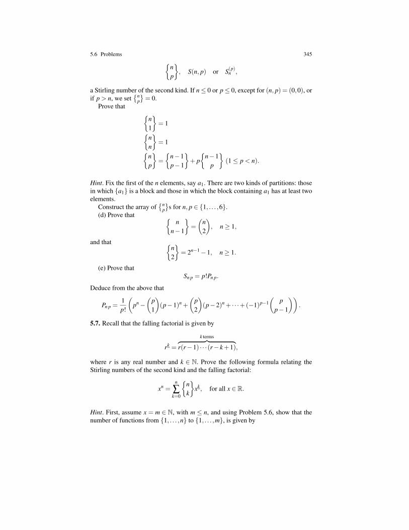
5.6 Problems 345np
, S(n, p) or S(p)
n ,
a Stirling number of the second kind. If n≤ 0 or p≤ 0, except for (n, p) = (0,0), orif p > n, we set
np
= 0.
Prove that n1
= 1
nn
= 1
np
=
n−1p−1
+ p
n−1p
(1≤ p < n).
Hint. Fix the first of the n elements, say a1. There are two kinds of partitions: thosein which a1 is a block and those in which the block containing a1 has at least twoelements.
Construct the array ofn
p
s for n, p ∈ 1, . . . ,6.
(d) Prove that n
n−1
=
(n2
), n≥ 1,
and that n2
= 2n−1−1, n≥ 1.
(e) Prove thatSn p = p!Pn p.
Deduce from the above that
Pn p =1p!
(pn−
(p1
)(p−1)n +
(p2
)(p−2)n + · · ·+(−1)p−1
(p
p−1
)).
5.7. Recall that the falling factorial is given by
rk =
k terms︷ ︸︸ ︷r(r−1) · · ·(r− k+1),
where r is any real number and k ∈ N. Prove the following formula relating theStirling numbers of the second kind and the falling factorial:
xn =n
∑k=0
nk
xk, for all x ∈ R.
Hint. First, assume x = m ∈ N, with m ≤ n, and using Problem 5.6, show that thenumber of functions from 1, . . . ,n to 1, . . . ,m, is given by
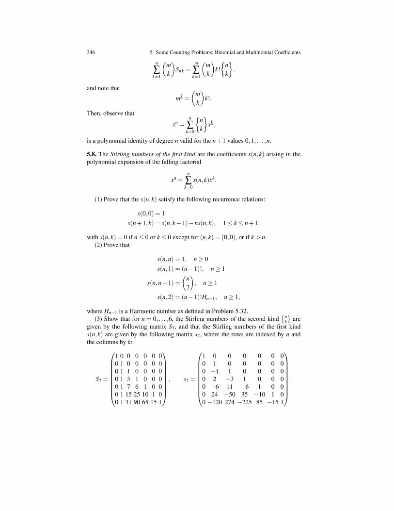
346 5 Some Counting Problems; Binomial and Multinomial Coefficients
n
∑k=1
(mk
)Snk =
m
∑k=1
(mk
)k!
nk
,
and note that
mk =
(mk
)k!.
Then, observe that
xn =n
∑k=0
nk
xk,
is a polynomial identity of degree n valid for the n+1 values 0,1, . . . ,n.
5.8. The Stirling numbers of the first kind are the coefficients s(n,k) arising in thepolynomial expansion of the falling factorial
xn =n
∑k=0
s(n,k)xk.
(1) Prove that the s(n,k) satisfy the following recurrence relations:
s(0,0) = 1s(n+1,k) = s(n,k−1)−ns(n,k), 1≤ k ≤ n+1,
with s(n,k) = 0 if n≤ 0 or k ≤ 0 except for (n,k) = (0,0), or if k > n.(2) Prove that
s(n,n) = 1, n≥ 0s(n,1) = (n−1)!, n≥ 1
s(n,n−1) =(
n2
), n≥ 1
s(n,2) = (n−1)!Hn−1, n≥ 1,
where Hn−1 is a Harmonic number as defined in Problem 5.32.(3) Show that for n = 0, . . . ,6, the Stirling numbers of the second kind
nk
are
given by the following matrix S7, and that the Stirling numbers of the first kinds(n,k) are given by the following matrix s7, where the rows are indexed by n andthe columns by k:
S7 =
1 0 0 0 0 0 00 1 0 0 0 0 00 1 1 0 0 0 00 1 3 1 0 0 00 1 7 6 1 0 00 1 15 25 10 1 00 1 31 90 65 15 1
, s7 =
1 0 0 0 0 0 00 1 0 0 0 0 00 −1 1 0 0 0 00 2 −3 1 0 0 00 −6 11 −6 1 0 00 24 −50 35 −10 1 00 −120 274 −225 85 −15 1
.
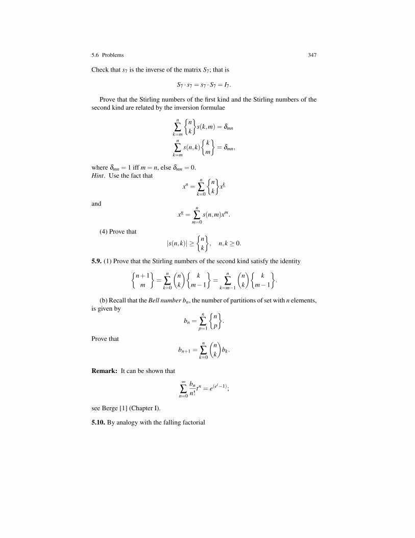
5.6 Problems 347
Check that s7 is the inverse of the matrix S7; that is
S7 · s7 = s7 ·S7 = I7.
Prove that the Stirling numbers of the first kind and the Stirling numbers of thesecond kind are related by the inversion formulae
n
∑k=m
nk
s(k,m) = δmn
n
∑k=m
s(n,k)
km
= δmn,
where δmn = 1 iff m = n, else δmn = 0.Hint. Use the fact that
xn =n
∑k=0
nk
xk
and
xn =n
∑m=0
s(n,m)xm.
(4) Prove that
|s(n,k)| ≥
nk
, n,k ≥ 0.
5.9. (1) Prove that the Stirling numbers of the second kind satisfy the identityn+1
m
=
n
∑k=0
(nk
)k
m−1
=
n
∑k=m−1
(nk
)k
m−1
.
(b) Recall that the Bell number bn, the number of partitions of set with n elements,is given by
bn =n
∑p=1
np
.
Prove that
bn+1 =n
∑k=0
(nk
)bk.
Remark: It can be shown that
∞
∑n=0
bn
n!tn = e(e
t−1);
see Berge [1] (Chapter I).
5.10. By analogy with the falling factorial
348 5 Some Counting Problems; Binomial and Multinomial Coefficients
rk =
k terms︷ ︸︸ ︷r(r−1) · · ·(r− k+1),
where r is any real number and k ∈ N, we can define the rising factorial
rk =
k terms︷ ︸︸ ︷r(r+1) · · ·(r+ k−1) .
We define the signless Stirling numbers of the first kind c(n,k), by
c(n,k) = (−1)n−ks(n,k),
where the s(n,k) are the (signed) Stirling numbers of the first kind. Observe thatc(n,k)≥ 0.
(1) Prove that the c(n,k) satisfy the following recurrence relations:
c(0,0) = 1c(n+1,k) = c(n,k−1)+nc(n,k), 1≤ k ≤ n+1,
with c(n,k) = 0 if n≤ 0 or k ≤ 0 except for (n,k) = (0,0), or if k > n.(2) Prove that
rn =n
∑k=0
c(n,k)rk;
that is, the c(n,k) are the coefficients of the polynomial rn.(3) Prove that the falling and the rising factorials are related as follows:
rn = (−1)n(−r)n.
5.11. In Problem 3.15, we defined a k-cycle (or cyclic permutation of order k) asa permutation σ : [n]→ [n] such that for some sequence (i1, i2, . . . , ik) of distinctelements of [n] with 2≤ k ≤ n,
σ(i1) = i2,σ(i2) = i3, . . . ,σ(ik−1) = ik,σ(ik) = i1
and σ( j) = j for all j ∈ [n]−i1, . . . , ik. The set i1, i2, . . . , ik is called the domainof the cyclic permutation. Then, we proved that for every permutation π : [n]→ [n],if π is not the identity, then π can be written as the composition
π = σ1 · · · σs
of cyclic permutations σ j with disjoint domains. Furthermore, the cyclic permuta-tions σ j are uniquely determined by the nontrivial orbits of Rπ (defined in Problem3.15), and an element m ∈ [n] is a fixed point of π iff m is not in the domain of anycycle σ j.
In the above definition of a k-cycle, we assumed that k ≥ 2, but in order to countthe number of permutations with i cycles, it is necessary to allow 1-cycles to account
5.6 Problems 349
for the fixed points of permutations. Consequently, we define a 1-cycle as any sin-gleton subset j of [n], and we call j the domain of the 1-cycle. As permutations,1-cycles all correspond to the identity permutation, but for the purpose of countingthe cycles of a permutation π , it is convenient to distinguish among the 1-cycles de-pending on which particular fixed point of π is singled out. Then the main result ofProblem 3.15 can be formulated as follows: every permutation π can be written in aunique way (up to order of the cycles) as the composition of k-cycles with disjointdomains
π = σ1 · · · σs σ j1 · · · σ jt ,
where σ1, . . . ,σs are k-cycles with k ≥ 2, and σ j1 , . . . ,σ jt are copies of the identitypermutation corresponding to the fixed points of π (π( jm) = jm for m = 1, . . . , t).
(i) Prove that the number c(n, i) of permutations of n elements consisting of ex-actly i cycles satisfies the following recurrence:
c(0,0) = 1c(n+1, i) = c(n, i−1)+nc(n, i), 1≤ i≤ n+1
c(0,n) = 0 n≥ 1c(n,0) = 0 n≥ 1.
(ii) Conclude that the signless Stirling numbers of the first kind count the numberof permutations of n elements with exactly i cycles.
(iii) Prove thatn
∑i=0
c(n, i) = n!, n ∈ N.
(iv) Consider all permutations π of [n] that can be written as a composition ofcycles, with λ1 cycles of length 1, λ2 cycles of length 2, ..., λk cycles of length k,where 1 ·λ1 +2 ·λ2 + · · ·+k ·λk = n. Prove that the number of such permutations isgiven by
h(λ1,λ2, . . . ,λk) =n!
1λ1 ·λ1! ·2λ2 ·λ2! · · ·kλk ·λk!,
a formula known as Cauchy’s formula.
5.12. The Fibonacci numbers Fn are defined recursively as follows.
F0 = 0F1 = 1
Fn+2 = Fn+1 +Fn, n≥ 0.
For example, 0,1,1,2,3,5,8,13,21,34,55, . . . are the first 11 Fibonacci numbers.Prove that
Fn+1 =
(n0
)+
(n−1
1
)+
(n−2
2
)+ · · ·+
(0n
).
350 5 Some Counting Problems; Binomial and Multinomial Coefficients
Hint. Use complete induction. Also, consider the two cases, n even and n odd.
5.13. Given any natural number, n ≥ 1, let pn denote the number of permutationsf : 1, . . . ,n→ 1, . . . ,n that leave no element fixed, that is, such that f (i) 6= i, forall i ∈ 1, . . . ,n. Such permutations are sometimes called derangements. Note thatp1 = 0 and set p0 = 1.
(a) Prove that
n! = pn +
(n1
)pn−1 +
(n2
)pn−2 + · · ·+
(nn
).
Hint. For every permutation f : 1, . . . ,n→ 1, . . . ,n, let
Fix( f ) = i ∈ 1, . . . ,n | f (i) = i
be the set of elements left fixed by f . Prove that there are pn−k permutations associ-ated with any fixed set Fix( f ) of cardinality k.
(b) Prove that
pn = n!(
1− 11!
+12!
+ · · ·+ (−1)k
k!+ · · ·+ (−1)n
n!
)= n!−
(n1
)(n−1)!+
(n2
)(n−2)!+ · · ·+(−1)n.
Hint. Use the same method as in Problem 5.5.Conclude from (b) that
limn→∞
pn
n!=
1e.
Hint. Recall that
ex = 1+x1!
+x2
2!+ · · ·+ xn
n!+ · · · .
Remark: The ratio pn/n! has an interesting interpretation in terms of probabili-ties. Assume n persons go to a restaurant (or to the theatre, etc.) and that they allcherk their coats. Unfortunately, the cleck loses all the coat tags. Then, pn/n! is theprobability that nobody will get her or his own coat back.
(c) Prove thatpn = npn−1 +(−1)n,
for all n≥ 1, with p0 = 1.Note that n! is defined by n! = n(n−1)!. So, pn is a sort of “weird factorial” with
a strange corrective term (−1)n.
5.14. Consider a sequence of n ≥ 2 items (not necessarily distinct), and assumethat m of them are (indistinguishable and) defective, the remaining n−m beingfunctional (also indistinguishable).
5.6 Problems 351
(1) Prove that the number of sequences of n items such that no two defectiveobjects are next to each other is (
n−m+1m
).
Hint. Let x1 be the number of items to the left of the first defective object, x2 thenumber of items between the first two defective objects, and so on. The list of itemsis described by the sequence
x1 0 x2 0 . . . xm 0 xm+1.
Observe that there will be a functional item between any pair of defectives iff xi > 0,for i = 2, . . . ,m.
(2) Assume n ≥ 3m−2. Prove that the number of sequences where each pair ofdefective items is separated by at least 2 functional items is(
n−2m+2m
).
5.15. Consider the integers 1,2, . . . ,n. For any any r ≥ 2 such that n≥ 2r−1, provethat the number of subsequences (x1, . . . ,xr) of 1,2, . . . ,n such that xi 6= xi+1 fori = 1, . . . ,r−1, is (
n− r+1r
).
Hint. Define y1, . . . ,yr+1 such that y1 = x1, yi = xi− xi−1− 1 for i = 2, . . . ,r, andyr+1 = n− xr−1, and observe that the yi must be positive solutions of the equation
y1 + · · ·+ yr+1 = n− r+2.
5.16. For all k,n ≥ 1, prove that the number of sequences (A1, . . . ,Ak) of (possiblyempty) subsets Ai ⊆ 1, . . . ,n such that
k⋃i=1
Ai = 1, . . . ,n,
is(2k−1)n.
Hint. Reduce this to counting the number of certain kinds of matrices with 0,1-entries.
5.17. Prove that if m+ p≥ n and m,n, p≥ 0, then(m+ p
n
)=
m
∑k=0
(mk
)(p
n− k
).
352 5 Some Counting Problems; Binomial and Multinomial Coefficients
Hint. Observe that(m+p
n
)is the coefficient of am+p−nbn in (a + b)m+p = (a +
b)m(a+b)p.Show that the above implies that if n≥ p, then(
m+ pn
)=
(m
n− p
)(pp
)+
(m
n− p+1
)(p
p−1
)+
(m
n− p+2
)(p
p−2
)+ · · ·+
(mn
)(p0
)and if n≤ p then(
m+ pn
)=
(m0
)(pn
)+
(m1
)(p
n−1
)+
(m2
)(p
n−2
)+ · · ·+
(mn
)(p0
).
5.18. Give combinatorial proofs for the following identities:(2nn
)= 2(
n2
)+n2 (a)
(m+n
r
)=
r
∑k=0
(mk
)(n
r− k
). (b)
5.19. Prove that (0m
)+
(1m
)+ · · ·+
(nm
)=
(n+1m+1
),
for all m,n ∈ N with 0≤ m≤ n.
5.20. Prove that(m0
)+
(m+1
1
)+ · · ·+
(m+n
n
)=
(m+n+1
n
).
5.21. Prove thatm
∑k=0
(−1)k(
nk
)= (−1)m
(n−1
m
),
if 0≤ m≤ n.
5.22. (1) Prove that (rk
)= (−1)k
(k− r−1
k
),
where r ∈ R and k ∈ Z (negating the upper index).(2) Use (1) and the identity of Problem 5.20 to prove that
m
∑k=0
(−1)k(
nk
)= (−1)m
(n−1
m
),
if 0≤ m≤ n.
5.6 Problems 353
5.23. Prove thatn
∑k=0
(nk
)(km
)= 2n−m
(mk
),
where 0≤ m≤ n.
5.24. Prove that
(1+ x)−12 = 1+
∞
∑k=1
(−1)k 1 ·3 ·5 · · ·(2k−1)2 ·4 ·6 · · ·2k
xk
= 1+∞
∑k=1
(−1)k(2k)!(k!)222k xk
= 1+∞
∑k=1
(−1)k
22k
(2kk
)xk
if |x|< 1.
5.25. Prove that
ln(1+ x)≤ x− x2
2+
x3
3,
for all x≥−1.
5.26. If n = 2m+1, prove that(2m+1
m
)∼√
2m+12πm(m+1)
(1+
12m
)m(1− 1
2(m+1)
)m+1
22m+1,
for m large and so, (2m+1
m
)∼√
2m+12πm(m+1)
22m+1,
for m large.
5.27. If n = 2m+1, prove that
e−t(t+1)/(m+1−t) ≤(
2m+1m− t
)/(2m+1
m
)≤ e−t(t+1)/(m+1+t)
with 0≤ t ≤ m. Deduce from this that(2m+1
k
)/(2m+1
m
)∼ e1/(4(m+1)) e−(2m+1−2k)2/(4(m+1)),
for m large and 0≤ k ≤ 2m+1.
5.28. Prove Proposition 5.17.

354 5 Some Counting Problems; Binomial and Multinomial Coefficients
Hint. First, show that the function
t 7→ t2
m+ t
is strictly increasing for t ≥ 0.
5.29. (1) Prove that
1−√
1−4x2x
= 1+∞
∑k=1
1k+1
(2kk
)xk.
(2) The numbers
Cn =1
n+1
(2nn
),
are known as the Catalan numbers (n≥ 0). The Catalan numbers are the solution ofmany counting problems in combinatorics. The Catalan sequence begins with
1, 1, 2, 5, 14, 42, 132, 429, 1430, 4862, 16796, . . . .
Prove that
Cn =
(2nn
)−(
2nn−1
)=
12n+1
(2n+1
n
).
(3) Prove that C0 = 1 and that
Cn+1 =2(2n+1)
n+2Cn.
(4) Prove that Cn is the number of ways a convex polygon with n+2 sides can besubdivided into triangles (triangulated) by connecting vertices of the polygon with(nonintersecting) line segments.Hint. Observe that any triangulation of a convex polygon with n+2 sides has n−1edges in addition to the sides of the polygon and thus, a total of 2n+1 edges. Provethat
(4n+2)Cn = (n+2)Cn+1.
(5) Prove that Cn is the number of full binary trees with n+1 leaves (a full binarytree is a tree in which every node has degree 0 or 2).
5.30. Which of the following expressions is the number of partitions of a set withn≥ 1 elements into two disjoint blocks:
(1) 2n−2 (2) 2n−1−1.
Justify your answer.
5.31. (1) If X is a finite set, prove that any function m : 2X → R+ such that, for allsubsets A,B of X , if A∩B = /0, then
5.6 Problems 355
m(A∪B) = m(A)+m(B), (∗)
induces a measure on X . This means that the function m′ : X → R+ given by
m′(x) = m(x), x ∈ X ,
gives m back, in the sense that for every subset A of X ,
m(A) = ∑x∈A
m′(x) = ∑x∈A
m(x).
Hint. First, prove that m( /0) = 0. Then, generalize (∗) to finite families of pairwisedisjoint subsets.
Show that m is monotonic, which means that for any two subsets A,B of X ifA⊆ B, then m(A)≤ m(B).
(2) Given any sequence A1, . . . ,An of subsets of a finite set X , for any measure mon X , prove that
m( n⋃
k=1
Ak
)= ∑
I⊆1,...,nI 6= /0
(−1)(|I|−1)m(⋂
i∈I
Ai
),
and
m( n⋂
k=1
Ak
)= ∑
I⊆1,...,nI 6= /0
(−1)(|I|−1)m(⋃
i∈I
Ai
).
5.32. Let Hn, called the nth harmonic number, be given by
Hn = 1+12+
13+ · · ·+ 1
n,
with n≥ 1.(a) Prove that Hn /∈N for all n≥ 2; that is, Hn is not a whole number for all n≥ 2.
Hint. First, prove that every sequence 1,2,3, . . . ,n, with n ≥ 2, contains a uniquenumber of the form 2kq, with k ≥ 1 as big as possible and q odd (q = 1 is possible),which means that for every other number of the form 2k′q′, with 2k′q′ 6= 2kq, 1 ≤2k′q′ ≤ n, k′ ≥ 1 and q′ odd, we must have k′ < k. Then, prove that the numerator ofHn is odd and that the denominator of Hn is even, for all n≥ 2.
(b) Prove that
H1 +H2 + · · ·+Hn = (n+1)(Hn+1−1) = (n+1)Hn−n.
(c) Prove thatln(n+1)≤ Hn,
for all n≥ 1.Hint. Use the fact that
356 5 Some Counting Problems; Binomial and Multinomial Coefficients
ln(1+ x)≤ x for all x >−1,
that
ln(n+1) = ln(n)+ ln(
1+1n
),
and compute the sumn
∑k=1
(1k− ln
(1+
1k
)).
Prove thatln(n)+
1n≤ Hn.
(d) Prove that
Hn ≤ ln(n+1)+12
n
∑k=1
1k2 = ln(n)+ ln
(1+
1n
)+
12
n
∑k=1
1k2 .
Hint. Use the fact that
ln(1+ x)≥ x− x2
2for all x, where 0≤ x≤ 1 (in fact, for all x≥ 0), and compute the sum
n
∑k=1
(ln(
1+1k
)− 1
k+
12k2
).
Show thatn
∑k=1
1k2 ≤ 2− 1
n,
and deduce thatHn ≤ 1+ ln(n)+
12n
.
Remark: Actually,∞
∑k=1
1k2 =
π2
6≈ 1.645,
and this can be used to prove that
Hn ≤ 1+ ln(n).
Indeed, prove that for n≥ 6,
ln(
1+1n
)+
π2
12≤ 1,
and that Hn ≤ 1+ ln(n) for n = 1, . . . ,5.
5.6 Problems 357
(e) It is known that ln(1 + x) is given by the following convergent series for|x|< 1,
ln(1+ x) = x− x2
2+
x3
3+ · · ·+(−1)n+1 xn
n+ · · · .
Deduce from this that
ln(
xx−1
)=
1x+
12x2 +
13x3 + · · ·+ 1
nxn + · · · .
for all x with |x|> 1.Let
H(r)n =
n
∑k=1
1kr .
If r > 1, it is known that each H(r)n converges to a limit denoted H(r)
∞ or ζ (r), whereζ is Riemann’s zeta function given by
ζ (r) =∞
∑k=1
1kr ,
for all r > 1.
Fig. 5.6 G. F. Bernhard Riemann, 1826–1866
Prove that
ln(n) =n
∑k=2
(1k+
12k2 +
13k3 + · · ·+ 1
mkm + · · ·)
= (Hn−1)+12(H(2)
n −1)+13(H(3)
n −1)+ · · ·+ 1m(H(m)
n −1)+ · · ·
and therefore,
Hn− ln(n) = 1− 12(H(2)
n −1)− 13(H(3)
n −1)−·· ·− 1m(H(m)
n −1)−·· · .
Remark: The right-hand side has the limit
358 5 Some Counting Problems; Binomial and Multinomial Coefficients
γ = 1− 12(ζ (2)−1)− 1
3(ζ (3)−1)−·· ·− 1
m(ζ (m)−1)−·· ·
known as Euler’s constant (or the Euler–Mascheroni number).
Fig. 5.7 Leonhard Euler, 1707–1783 (left) and Jacob Bernoulli, 1654–1705 (right)
It is known thatγ = 0.577215664901 · · ·
but we don’t even know whether γ is irrational! It can be shown that
Hn = ln(n)+ γ +1
2n− 1
12n2 +εn
120n4 ,
with 0 < εn < 1.
5.33. The purpose of this problem is to derive a formula for the sum
Sk(n) = 1k +22 +3k + · · ·+nk
in terms of a polynomial in n (where k,n≥ 1 and n≥ 0, with the understanding thatthis sum is 0 when n = 0). Such a formula was derived by Jacob Bernoulli (1654–1705) and is expressed in terms of certain numbers now called Bernoulli numbers.
The Bernoulli numbers Bk are defined inductively by solving some equationslisted below,
B0 = 1B2−2B1 +1 = B2
B3−3B2 +3B1−1 = B3
B4−4B3 +6B2−4B1 +1 = B4
B5−5B4 +10B3−10B2 +5B1−1 = B5
and, in general,k
∑i=0
(ki
)(−1)iBk−i = Bk, k ≥ 2.

5.6 Problems 359
Because B1, . . . ,Bk−2 are known inductively, this equation can be used to computeBk−1.
Remark: It should be noted that there is more than one definition of the Bernoullinumbers. There are two main versions that differ in the choice of B1:
1. B1 = 12
2. B1 =− 12 .
The first version is closer to Bernoulli’s original definition and we find it moreconvenient for stating the identity for Sk(n) but the second version is probably usedmore often and has its own advantages.
(a) Prove that the first 14 Bernoulli numbers are the numbers listed below:
n 0 1 2 3 4 5 6 7 8 9 10 11 12 13 14
Bn 1 12
16 0 −1
30 0 142 0 −1
30 0 566 0 −691
2730 0 76
Observe two patterns:
1. All Bernoulli numbers B2k+1, with k ≥ 1, appear to be zero.2. The signs of the Bernoulli numbers Bn, alternate for n≥ 2.
The above facts are indeed true but not so easy to prove from the defining equations.However, they follow fairly easily from the fact that the generating function of thenumbers
Bk
k!can be computed explicitly in terms of the exponential function.
(b) Prove thatz
1− e−z =∞
∑k=0
Bk zk
k!.
Hint. Expand z/(1− e−z) into a power series
z1− e−z =
∞
∑k=0
bkzk
k!
near 0, multiply both sides by 1−e−z, and equate the coefficients of zk+1; from this,prove that bk = Bk for all k ≥ 0.
Remark: If we define B1 =− 12 , then we get
zez−1
=∞
∑k=0
Bk zk
k!.
(c) Prove that B2k+1 = 0, for all k ≥ 1.Hint. Observe that

360 5 Some Counting Problems; Binomial and Multinomial Coefficients
z1− e−z −
z2=
z(ez +1)2(ez−1)
= 1+∞
∑k=2
Bk zk
k!
is an even function (which means that it has the same value when we change z to−z).
(d) Define the Bernoulli polynomial Bk(x) by
Bk(x) =k
∑i=0
(ki
)xk−iBi,
for every k ≥ 0. Prove that
Bk+1(n)−Bk+1(n−1) = (k+1)nk,
for all k ≥ 0 and all n≥ 1. Deduce from the above identities that
Sk(n) =1
k+1(Bk+1(n)−Bk+1(0)) =
1k+1
k
∑i=0
(k+1
i
)nk+1−iBi,
an identity often known as Bernoulli’s formula.Hint. Expand (n−1)k+1−i using the binomial formula and use the fact that(
mi
)(m− i
j
)=
(m
i+ j
)(i+ j
i
).
Remark: If we assume that B1 =− 12 , then
Bk+1(n+1)−Bk+1(n) = (k+1)nk.
Find explicit formulae for S4(n) and S5(n).
Extra Credit. It is reported that Euler computed the first 30 Bernoulli numbers.Prove that
B20 =−174611
330, B32 =
−7709321041217510
.
What does the prime 37 have to do with the numerator of B32?
Remark: Because
z1− e−z −
z2=
z(ez +1)2(ez−1)
=z2
ez/2 + e−z/2
ez/2− e−z/2 =z2
coth( z
2
),
where coth is the hyperbolic tangent function given by
coth(z) =coshzsinhz
,
with
5.6 Problems 361
coshz =ez + e−z
2, sinhz =
ez− e−z
2.
It follows that
zcothz =2z
1− e−2z − z =∞
∑k=0
B2k (2z)2k
(2k)!=
∞
∑k=0
4kB2k z2k
(2k)!.
If we use the fact that
sinz =−i sinh iz, cosz = coshiz,
we deduce that cotz = cosz/sinz = i coth iz, which yields
zcotz =∞
∑k=0
(−4)kB2k z2k
(2k)!.
Now, Euler found the remarkable formula
zcotz = 1−2∞
∑k=1
z2
k2π2− z2 .
By expanding the right-hand side of the above formula in powers of z2 and equatingthe coefficients of z2k in both series for z cotz, we get the amazing formula:
ζ (2k) = (−1)k−1 22k−1π2k
(2k)!B2k,
for all k ≥ 1, where ζ (r) is Riemann’s zeta function given by
ζ (r) =∞
∑n=1
1nr ,
for all r > 1. Therefore, we get
B2k = ζ (2k)(−1)k−1 (2k)!22k−1π2k = (−1)k−12(2k)!
∞
∑n=1
1(2πn)2k ,
a formula due to due to Euler. This formula shows that the signs of the B2k alternatefor all k ≥ 1. Using Stirling’s formula, it also shows that
|B2k| ∼ 4√
πk(
kπe
)2k
so B2k tends to infinity rather quickly when k goes to infinity.
5.34. The purpose of this problem is to derive a recurrence formula for the sum
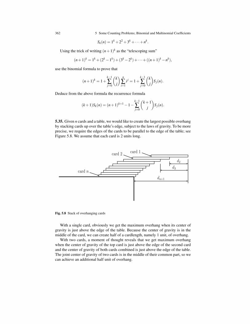
362 5 Some Counting Problems; Binomial and Multinomial Coefficients
Sk(n) = 1k +22 +3k + · · ·+nk.
Using the trick of writing (n+1)k as the “telescoping sum”
(n+1)k = 1k +(2k−1k)+(3k−2k)+ · · ·+((n+1)k−nk),
use the binomial formula to prove that
(n+1)k = 1+k−1
∑j=0
(kj
) n
∑i=1
i j = 1+k−1
∑j=0
(kj
)S j(n).
Deduce from the above formula the recurrence formula
(k+1)Sk(n) = (n+1)k+1−1−k−1
∑j=0
(k+1
j
)S j(n).
5.35. Given n cards and a table, we would like to create the largest possible overhangby stacking cards up over the table’s edge, subject to the laws of gravity. To be moreprecise, we require the edges of the cards to be parallel to the edge of the table; seeFigure 5.8. We assume that each card is 2 units long.
1
d2
d3
dn+1
card 1card 2
card n
Fig. 5.8 Stack of overhanging cards
With a single card, obviously we get the maximum overhang when its center ofgravity is just above the edge of the table. Because the center of gravity is in themiddle of the card, we can create half of a cardlength, namely 1 unit, of overhang.
With two cards, a moment of thought reveals that we get maximum overhangwhen the center of gravity of the top card is just above the edge of the second cardand the center of gravity of both cards combined is just above the edge of the table.The joint center of gravity of two cards is in the middle of their common part, so wecan achieve an additional half unit of overhang.

5.6 Problems 363
Given n cards, we find that we place the cards so that the center of gravity ofthe top k cards lies just above the edge of the (k+ 1)st card (which supports thesetop k cards). The table plays the role of the (n + 1)st card. We can express thiscondition by defining the distance dk from the extreme edge of the topmost cardto the corresponding edge of the kth card from the top (see Figure 5.8). Note thatd1 = 0. In order for dk+1 to be the center of gravity of the first k cards, we must have
dk+1 =(d1 +1)+(d2 +2)+ · · ·+(dk +1)
k,
for 1 ≤ k ≤ n. This is because the center of gravity of k objects having respectiveweights w1, . . . ,wk and having respective centers of gravity at positions x1, . . . ,xk isat position
w1x1 +w2x2 + · · ·+wkxk
w1 +w2 + · · ·+wk.
Prove that the equations defining the dk+1 imply that
dk+1 = dk +1k,
and thus, deduce that
dk+1 = Hk = 1+12+
13+ · · ·+ 1
k,
the kth Harmonic number (see Problem 5.32). Conclude that the total overhang withn cards is Hn.
Prove that it only takes four cards to achieve an overhang of one cardlength. Whatkind of overhang (in terms of cardlengths) is achieved with 52 cards? (See the endof Problem 5.32.)
5.36. Consider n≥ 2 lines in the plane. We say that these lines are in general posi-tion iff no two of them are parallel and no three pass through the same point. Provethat n lines in general position divide the plane into
n(n+1)2
+1
regions.
5.37. (A deceptive induction, after Conway and Guy [3]) Place n distinct pointson a circle and draw the line segments joining all pairs of these points. These linesegments determine some regions inside the circle as shown in Figure 5.9 for fivepoints. Assuming that the points are in general position, which means that no morethan two line segments pass through any point inside the circle, we would like tocompute the number of regions inside the circle. These regions are convex and theirboundaries are line segments or possibly one circular arc.
If we look at the first five circles in Figure 5.10, we see that the number of regionsis
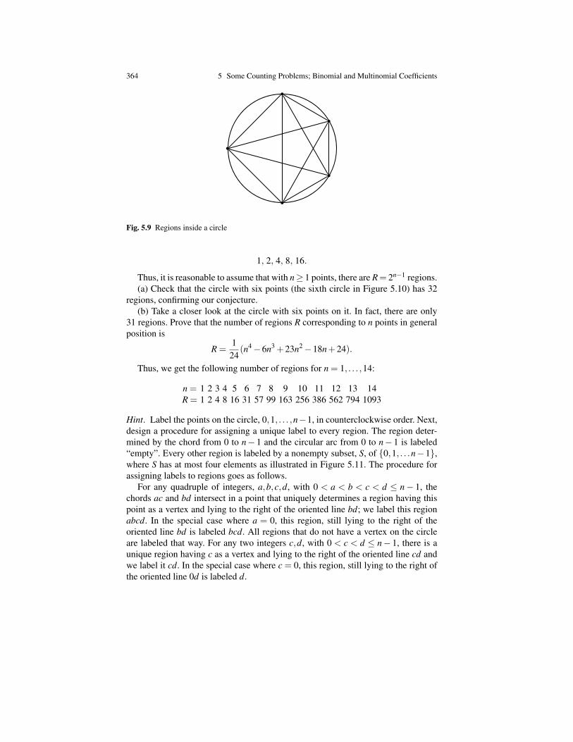
364 5 Some Counting Problems; Binomial and Multinomial Coefficients
1
Fig. 5.9 Regions inside a circle
1, 2, 4, 8, 16.
Thus, it is reasonable to assume that with n≥ 1 points, there are R= 2n−1 regions.(a) Check that the circle with six points (the sixth circle in Figure 5.10) has 32
regions, confirming our conjecture.(b) Take a closer look at the circle with six points on it. In fact, there are only
31 regions. Prove that the number of regions R corresponding to n points in generalposition is
R =124
(n4−6n3 +23n2−18n+24).
Thus, we get the following number of regions for n = 1, . . . ,14:
n = 1 2 3 4 5 6 7 8 9 10 11 12 13 14R = 1 2 4 8 16 31 57 99 163 256 386 562 794 1093
Hint. Label the points on the circle, 0,1, . . . ,n−1, in counterclockwise order. Next,design a procedure for assigning a unique label to every region. The region deter-mined by the chord from 0 to n− 1 and the circular arc from 0 to n− 1 is labeled“empty”. Every other region is labeled by a nonempty subset, S, of 0,1, . . .n−1,where S has at most four elements as illustrated in Figure 5.11. The procedure forassigning labels to regions goes as follows.
For any quadruple of integers, a,b,c,d, with 0 < a < b < c < d ≤ n− 1, thechords ac and bd intersect in a point that uniquely determines a region having thispoint as a vertex and lying to the right of the oriented line bd; we label this regionabcd. In the special case where a = 0, this region, still lying to the right of theoriented line bd is labeled bcd. All regions that do not have a vertex on the circleare labeled that way. For any two integers c,d, with 0 < c < d ≤ n− 1, there is aunique region having c as a vertex and lying to the right of the oriented line cd andwe label it cd. In the special case where c = 0, this region, still lying to the right ofthe oriented line 0d is labeled d.
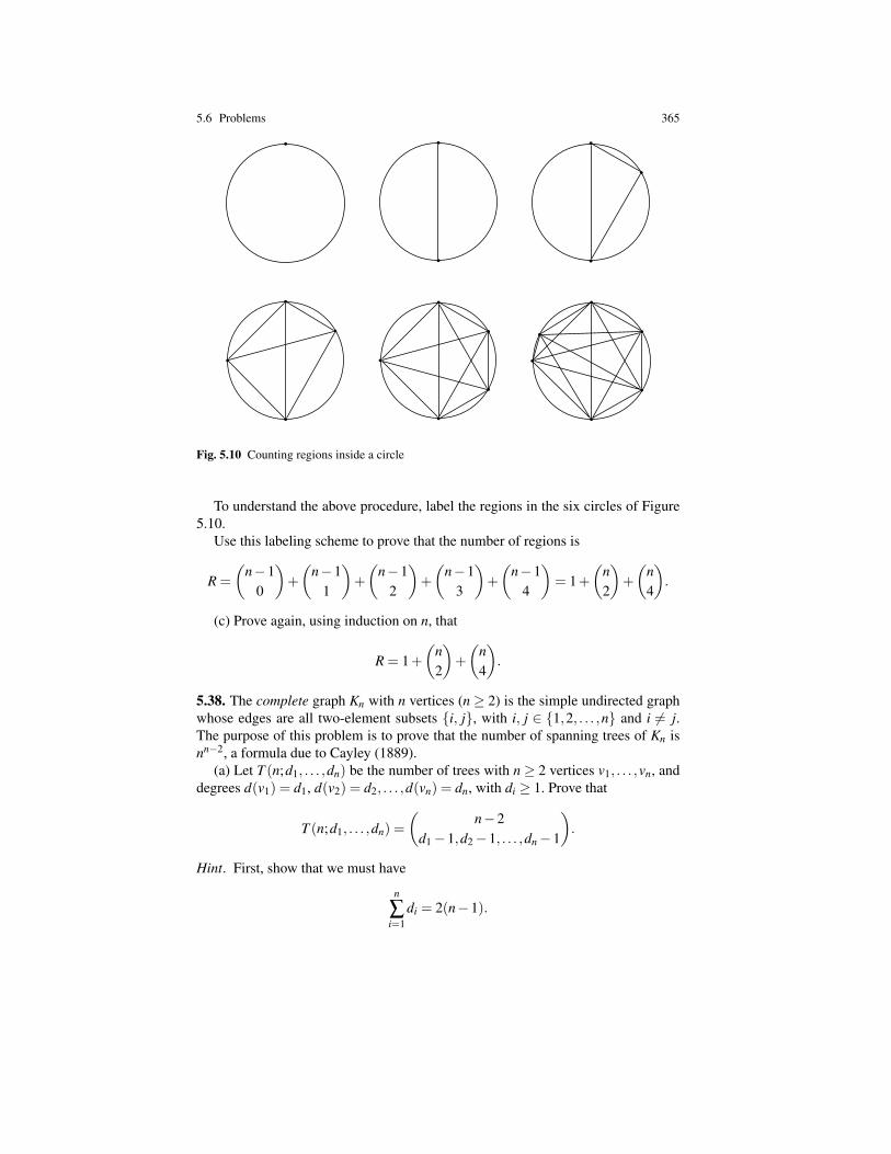
5.6 Problems 365
1 1 1
1 1 1
Fig. 5.10 Counting regions inside a circle
To understand the above procedure, label the regions in the six circles of Figure5.10.
Use this labeling scheme to prove that the number of regions is
R =
(n−1
0
)+
(n−1
1
)+
(n−1
2
)+
(n−1
3
)+
(n−1
4
)= 1+
(n2
)+
(n4
).
(c) Prove again, using induction on n, that
R = 1+(
n2
)+
(n4
).
5.38. The complete graph Kn with n vertices (n≥ 2) is the simple undirected graphwhose edges are all two-element subsets i, j, with i, j ∈ 1,2, . . . ,n and i 6= j.The purpose of this problem is to prove that the number of spanning trees of Kn isnn−2, a formula due to Cayley (1889).
(a) Let T (n;d1, . . . ,dn) be the number of trees with n≥ 2 vertices v1, . . . ,vn, anddegrees d(v1) = d1, d(v2) = d2, . . . ,d(vn) = dn, with di ≥ 1. Prove that
T (n;d1, . . . ,dn) =
(n−2
d1−1,d2−1, . . . ,dn−1
).
Hint. First, show that we must have
n
∑i=1
di = 2(n−1).
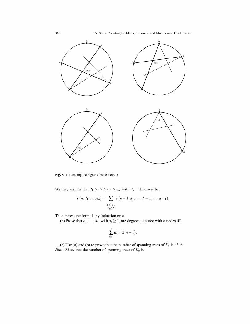
366 5 Some Counting Problems; Binomial and Multinomial Coefficients
1
0
a
b
c
d
abcd
1
0
b
c
d
bcd1
0
c
d
cd
1
0
d
d
Fig. 5.11 Labeling the regions inside a circle
We may assume that d1 ≥ d2 ≥ ·· · ≥ dn, with dn = 1. Prove that
T (n;d1, . . . ,dn) = ∑i
1≤i≤ndi≥2
T (n−1;d1, . . . ,di−1, . . . ,dn−1).
Then, prove the formula by induction on n.(b) Prove that d1, . . . ,dn, with di ≥ 1, are degrees of a tree with n nodes iff
n
∑i=1
di = 2(n−1).
(c) Use (a) and (b) to prove that the number of spanning trees of Kn is nn−2.Hint. Show that the number of spanning trees of Kn is
References 367
∑d1,...,dn≥1
d1+···+dn=2(n−1)
(n−2
d1−1,d2−1, . . . ,dn−1
)
and use the multinomial formula.
References
1. Claude Berge. Principles of Combinatorics. New York: Academic Press, first edition, 1971.2. J. Cameron, Peter. Combinatorics: Topics, Techniques, Algorithms. Cambridge, UK: Cam-
bridge University Press, first edition, 1994.3. John H. Conway and Richard K. Guy, The Book of Numbers. Copernicus, New York:
Springer-Verlag, first edition, 1996.4. Ronald L. Graham, Donald E. Knuth, and Oren Patashnik. Concrete Mathematics: A Foun-
dation For Computer Science. Reading, MA: Addison Wesley, second edition, 1994.5. L. Lovasz, J. Pelikan, and K. Vesztergombi. Discrete Mathematics. Elementary and Beyond.
Undergraduate Texts in Mathematics. New York: Springer, first edition, 2003.6. Jiri Matousek. Lectures on Discrete Geometry. GTM No. 212. New York: Springer Verlag,
first edition, 2002.7. Richard P. Stanley. Enumerative Combinatorics, Vol. I. Cambridge Studies in Advanced
Mathematics, No. 49. Cambridge UK: Cambridge University Press, first edition, 1997.8. J.H. van Lint and R.M. Wilson. A Course in Combinatorics. Cambridge UK: Cambridge
University Press, second edition, 2001.


Chapter 6An Introduction to Discrete Probability
6.1 Sample Space, Outcomes, Events, Probability
Roughly speaking, probability theory deals with experiments whose outcome arenot predictable with certainty. We often call such experiments random experiments.They are subject to chance. Using a mathematical theory of probability, we may beable to calculate the likelihood of some event.
In the introduction to his classical book [1] (first published in 1888), JosephBertrand (1822–1900) writes (translated from French to English):
“How dare we talk about the laws of chance (in French: le hasard)? Isn’t chancethe antithesis of any law? In rejecting this definition, I will not propose anyalternative. On a vaguely defined subject, one can reason with authority. ...”
Of course, Bertrand’s words are supposed to provoke the reader. But it does seemparadoxical that anyone could claim to have a precise theory about chance! It is notmy intention to engage in a philosophical discussion about the nature of chance.Instead, I will try to explain how it is possible to build some mathematical tools thatcan be used to reason rigorously about phenomema that are subject to chance. Thesetools belong to probability theory. These days, many fields in computer sciencesuch as machine learning, cryptography, computational linguistics, computer vision,robotics, and of course algorithms, rely a lot on probability theory. These fields arealso a great source of new problems that stimulate the discovery of new methodsand new theories in probability theory.
Although this is an oversimplification that ignores many important contributors,one might say that the development of probability theory has gone through four eraswhose key figures are: Pierre de Fermat and Blaise Pascal, Pierre–Simon Laplace,and Andrey Kolmogorov. Of course, Gauss should be added to the list; he mademajor contributions to nearly every area of mathematics and physics during his life-time. To be fair, Jacob Bernoulli, Abraham de Moivre, Pafnuty Chebyshev, Alek-sandr Lyapunov, Andrei Markov, Emile Borel, and Paul Levy should also be addedto the list.
369
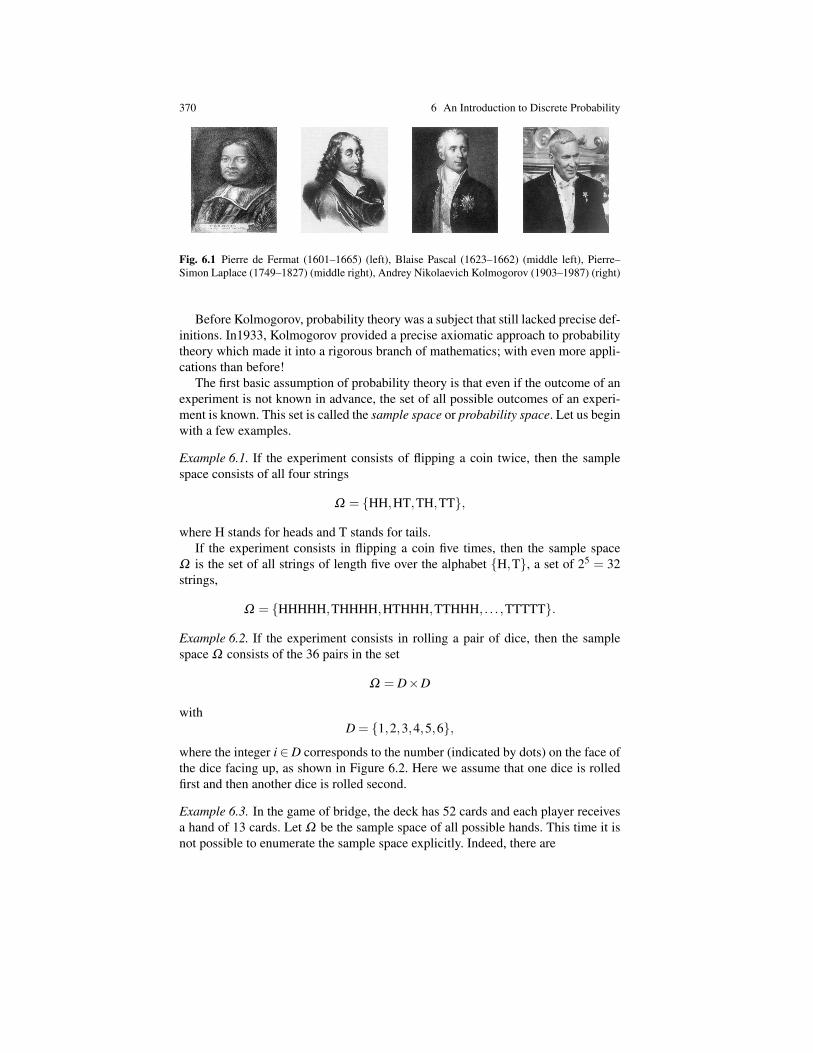
370 6 An Introduction to Discrete Probability
Fig. 6.1 Pierre de Fermat (1601–1665) (left), Blaise Pascal (1623–1662) (middle left), Pierre–Simon Laplace (1749–1827) (middle right), Andrey Nikolaevich Kolmogorov (1903–1987) (right)
Before Kolmogorov, probability theory was a subject that still lacked precise def-initions. In1933, Kolmogorov provided a precise axiomatic approach to probabilitytheory which made it into a rigorous branch of mathematics; with even more appli-cations than before!
The first basic assumption of probability theory is that even if the outcome of anexperiment is not known in advance, the set of all possible outcomes of an experi-ment is known. This set is called the sample space or probability space. Let us beginwith a few examples.
Example 6.1. If the experiment consists of flipping a coin twice, then the samplespace consists of all four strings
Ω = HH,HT,TH,TT,
where H stands for heads and T stands for tails.If the experiment consists in flipping a coin five times, then the sample space
Ω is the set of all strings of length five over the alphabet H,T, a set of 25 = 32strings,
Ω = HHHHH,THHHH,HTHHH,TTHHH, . . . ,TTTTT.
Example 6.2. If the experiment consists in rolling a pair of dice, then the samplespace Ω consists of the 36 pairs in the set
Ω = D×D
withD = 1,2,3,4,5,6,
where the integer i ∈D corresponds to the number (indicated by dots) on the face ofthe dice facing up, as shown in Figure 6.2. Here we assume that one dice is rolledfirst and then another dice is rolled second.
Example 6.3. In the game of bridge, the deck has 52 cards and each player receivesa hand of 13 cards. Let Ω be the sample space of all possible hands. This time it isnot possible to enumerate the sample space explicitly. Indeed, there are

6.1 Sample Space, Outcomes, Events, Probability 371
Fig. 6.2 Two dice
(5213
)=
52!13! ·39!
=52 ·51 ·50 · · ·4013 ·12 · · · ·2 ·1 = 635,013,559,600
different hands, a huge number.
Each member of a sample space is called an outcome or an elementary event.Typically, we are interested in experiments consisting of a set of outcomes. Forexample, in Example 6.1 where we flip a coin five times, the event that exactly oneof the coins shows heads is
A = HTTTT,THTTT,TTHTT,TTTHT,TTTTH.
The event A consists of five outcomes. In Example 6.3, the event that we get “dou-bles” when we roll two dice, namely that each dice shows the same value is,
B = (1,1),(2,2),(3,3),(4,4),(5,5),(6,6),
an event consisting of 6 outcomes.The second basic assumption of probability theory is that every outcome ω of
a sample space Ω is assigned some probability Pr(ω). Intuitively, Pr(ω) is theprobabilty that the outcome ω may occur. It is convenient to normalize probabilites,so we require that
0≤ Pr(ω)≤ 1.
If Ω is finite, we also require that
∑ω∈Ω
Pr(ω) = 1.
The function Pr is often called a probability distribution on Ω . Indeed, it distributesthe probability of 1 among the outomes ω .
In many cases, we assume that the probably distribution is uniform, which meansthat every outcome has the same probability.
For example, if we assume that our coins are “fair,” then when we flip a coin fivetimes, since each outcome in Ω is equally likely, the probability of each outcomeω ∈Ω is
Pr(ω) =1
32.

372 6 An Introduction to Discrete Probability
If we assume that our dice are “fair,” namely that each of the six possibilities for aparticular dice has probability 1/6 , then each of the 36 rolls ω ∈Ω has probability
Pr(ω) =1
36.
We can also consider “loaded dice” in which there is a different distribution ofprobabilities. For example, let
Pr1(1) = Pr1(6) =14
Pr1(2) = Pr1(3) = Pr1(4) = Pr1(5) =18.
These probabilities add up to 1, so Pr1 is a probability distribution on D. We canassign probabilities to the elements of Ω = D×D by the rule
Pr11(d,d′) = Pr1(d)Pr1(d′).
We can easily check that∑
ω∈Ω
Pr11(ω) = 1,
so Pr11 is indeed a probability distribution on Ω . For example, we get
Pr11(6,3) = Pr1(6)Pr1(3) =14· 1
8=
132
.
Let us summarize all this with the following definition.
Definition 6.1. A finite discrete probability space (or finite discrete sample space)is a finite set Ω of outcomes or elementary events ω ∈ Ω , together with a functionPr : Ω → R, called probability measure (or probability distribution) satisfying thefollowing properties:
0≤ Pr(ω)≤ 1 for all ω ∈Ω .
∑ω∈Ω
Pr(ω) = 1.
An event is any subset A of Ω . The probability of an event A is defined as
Pr(A) = ∑ω∈A
Pr(ω).
Definition 6.1 immediately implies that
Pr( /0) = 0Pr(Ω) = 1.

6.1 Sample Space, Outcomes, Events, Probability 373
For another example, if we consider the event
A = HTTTT,THTTT,TTHTT,TTTHT,TTTTH
that in flipping a coin five times, heads turns up exactly once, the probability of thisevent is
Pr(A) =5
32.
If we use the probability distribution Pr on the sample space Ω of pairs of dice, theprobability of the event of having doubles
B = (1,1),(2,2),(3,3),(4,4),(5,5),(6,6),
isPr(B) = 6 · 1
36=
16.
However, using the probability distribution Pr11, we obtain
Pr11(B) =116
+1
64+
164
+1
64+
164
+1
16=
316
>1
16.
Loading the dice makes the event “having doubles” more probable.It should be noted that a definition slightly more general than Definition 6.1 is
needed if we want to allow Ω to be infinite. In this case, the following definition isused.
Definition 6.2. A discrete probability space (or discrete sample space) is a triple(Ω ,F ,Pr) consisting of:
1. A nonempty countably infinite set Ω of outcomes or elementary events.2. The set F of all subsets of Ω , called the set of events.3. A function Pr : F →R, called probability measure (or probability distribution)
satisfying the following properties:
a. (positivity)0≤ Pr(A)≤ 1 for all A ∈F .
b. (normalization)Pr(Ω) = 1.
c. (additivity and continuity)For any sequence of pairwise disjoint events E1,E2, . . . ,Ei, . . . in F (whichmeans that Ei∩E j = /0 for all i 6= j), we have
Pr
(∞⋃
i=1
Ei
)=
∞
∑i=1
Pr(Ei).
The main thing to observe is that Pr is now defined directly on events, sinceevents may be infinite. The third axiom of a probability measure implies that
374 6 An Introduction to Discrete Probability
Pr( /0) = 0.
The notion of a discrete probability space is sufficient to deal with most problemsthat a computer scientist or an engineer will ever encounter. However, there arecertain problems for which it is necessary to assume that the family F of eventsis a proper subset of the power set of Ω . In this case, F is called the family ofmeasurable events, and F has certain closure properties that make it a σ -algebra(also called a σ -field). Some problems even require Ω to be uncountably infinite. Inthis case, we drop the word discrete from discrete probability space.
Remark: A σ -algebra is a nonempty family F of subsets of Ω satisfying the fol-lowing properties:
1. /0 ∈F .2. For every subset A⊆Ω , if A ∈F then A ∈F .3. For every countable family (Ai)i≥1 of subsets Ai ∈F , we have
⋃i≥1 Ai ∈F .
Note that every σ -algebra is a Boolean algebra (see Section 7.11, Definition 7.14),but the closure property (3) is very strong and adds spice to the story.
In this chapter, we deal mostly with finite discrete probability spaces, and occa-sionally with discrete probability spaces with a countably infinite sample space. Inthis latter case, we always assume that F = 2Ω , and for notational simplicity weomit F (that is, we write (Ω ,Pr) instead of (Ω ,F ,Pr)).
Because events are subsets of the sample space Ω , they can be combined usingthe set operations, union, intersection, and complementation. If the sample spaceΩ is finite, the definition for the probability Pr(A) of an event A ⊆ Ω given inDefinition 6.1 shows that if A,B are two disjoint events (this means that A∩B = /0),then
Pr(A∪B) = Pr(A)+Pr(B).
More generally, if A1, . . . ,An are any pairwise disjoint events, then
Pr(A1∪·· ·∪An) = Pr(A1)+ · · ·+Pr(An).
It is natural to ask whether the probabilities Pr(A∪B), Pr(A∩B) and Pr(A) canbe expressed in terms of Pr(A) and Pr(B), for any two events A,B ∈ Ω . In the firstand the third case, we have the following simple answer.
Proposition 6.1. Given any (finite) discrete probability space (Ω ,Pr), for any twoevents A,B⊆Ω , we have
Pr(A∪B) = Pr(A)+Pr(B)−Pr(A∩B)
Pr(A) = 1−Pr(A).
Furthermore, if A⊆ B, then Pr(A)≤ Pr(B).
Proof . Observe that we can write A∪B as the following union of pairwise disjointsubsets:

6.1 Sample Space, Outcomes, Events, Probability 375
A∪B = (A∩B)∪ (A−B)∪ (B−A).
Then, using the observation made just before Proposition 6.1, since we have the dis-joint unions A = (A∩B)∪ (A−B) and B = (A∩B)∪ (B−A), using the disjointnessof the various subsets, we have
Pr(A∪B) = Pr(A∩B)+Pr(A−B)+Pr(B−A)
Pr(A) = Pr(A∩B)+Pr(A−B)
Pr(B) = Pr(A∩B)+Pr(B−A),
and from these we obtain
Pr(A∪B) = Pr(A)+Pr(B)−Pr(A∩B).
The equation Pr(A) = 1−Pr(A) follows from the fact that A∩A = /0 and A∪A = Ω ,so
1 = Pr(Ω) = Pr(A)+Pr(A).
If A ⊆ B, then A∩B = A, so B = (A∩B)∪ (B−A) = A∪ (B−A), and since A andB−A are disjoint, we get
Pr(B) = Pr(A)+Pr(B−A).
Since probabilities are nonegative, the above implies that Pr(A)≤ Pr(B). ut
Remark: Proposition 6.1 still holds when Ω is infinite as a consequence of axioms(a)–(c) of a probability measure. Also, the equation
Pr(A∪B) = Pr(A)+Pr(B)−Pr(A∩B)
can be generalized to any sequence of n events. In fact, we already showed this asthe Principle of Inclusion–Exclusion, Version 2 (Theorem 5.2).
The following proposition expresses a certain form of continuity of the functionPr.
Proposition 6.2. Given any probability space (Ω ,F ,Pr) (discrete or not), for anysequence of events (Ai)i≥1, if Ai ⊆ Ai+1 for all i≥ 1, then
Pr
( ∞⋃i=1
Ai
)= lim
n7→∞Pr(An).
Proof . The trick is to express⋃
∞i=1 Ai as a union of pairwise disjoint events. Indeed,
we have
∞⋃i=1
Ai = A1∪ (A2−A1)∪ (A3−A2)∪·· ·∪ (Ai+1−Ai)∪·· · ,
so by property (c) of a probability measure
376 6 An Introduction to Discrete Probability
Pr
( ∞⋃i=1
Ai
)= Pr
(A1∪
∞⋃i=1
(Ai+1−Ai)
)= Pr(A1)+
∞
∑i=1
Pr(Ai+1−Ai)
= Pr(A1)+ limn7→∞
n−1
∑i=1
Pr(Ai+1−Ai)
= limn7→∞
Pr(An),
as claimed.
We leave it as an exercise to prove that if Ai+1 ⊆ Ai for all i≥ 1, then
Pr
( ∞⋂i=1
Ai
)= lim
n7→∞Pr(An).
In general, the probability Pr(A∩B) of the event A∩B cannot be expressed in asimple way in terms of Pr(A) and Pr(B). However, in many cases we observe thatPr(A∩B) = Pr(A)Pr(B). If this holds, we say that A and B are independent.
Definition 6.3. Given a discrete probability space (Ω ,Pr), two events A and B areindependent if
Pr(A∩B) = Pr(A)Pr(B).
Two events are dependent if they are not independent.
For example, in the sample space of 5 coin flips, we have the events
A = HHw | w ∈ H,T3∪HTw | w ∈ H,T3,
the event in which the first flip is H, and
B = HHw | w ∈ H,T3∪THw | w ∈ H,T3,
the event in which the second flip is H. Since A and B contain 16 outcomes, we have
Pr(A) = Pr(B) =1632
=12.
The intersection of A and B is
A∩B = HHw | w ∈ H,T3,
the event in which the first two flips are H, and since A∩B contains 8 outcomes, wehave
Pr(A∩B) =8
32=
14.
Since
6.1 Sample Space, Outcomes, Events, Probability 377
Pr(A∩B) =14
andPr(A)Pr(B) =
12· 1
2=
14,
we see that A and B are independent events. On the other hand, if we consider theevents
A = TTTTT,HHTTTand
B = TTTTT,HTTTT,we have
Pr(A) = Pr(B) =2
32=
116
,
and sinceA∩B = TTTTT,
we havePr(A∩B) =
132
.
It follows thatPr(A)Pr(B) =
116· 1
16=
1256
,
butPr(A∩B) =
132
,
so A and B are not independent.
Example 6.4. We close this section with a classical problem in probability known asthe birthday problem. Consider n < 365 individuals and assume for simplicity thatnobody was born on February 29. In this problem, the sample space is the set ofall 365n possible choices of birthdays for n individuals, and let us assume that theyare all equally likely. This is equivalent to assuming that each of the 365 days ofthe year is an equally likely birthday for each individual, and that the assignmentsof birthdays to distinct people are independent. Note that this does not take twinsinto account! What is the probability that two (or more) individuals have the samebirthday?
To solve this problem, it is easier to compute the probability that no two individ-uals have the same birthday. We can choose n distinct birthdays in
(365n
)ways, and
these can be assigned to n people in n! ways, so there are(365
n
)n! = 365 ·364 · · ·(365−n+1)
configurations where no two people have the same birthday. There are 365n possiblechoices of birthdays, so the probabilty that no two people have the same birthday is
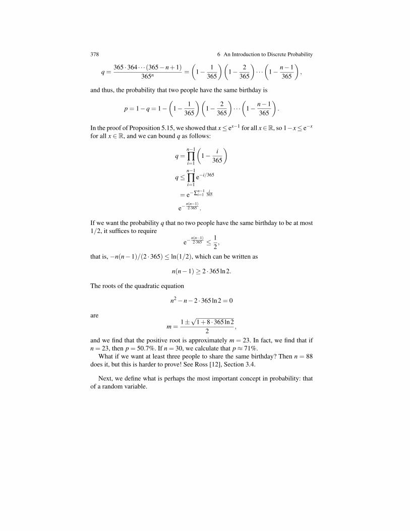
378 6 An Introduction to Discrete Probability
q =365 ·364 · · ·(365−n+1)
365n =
(1− 1
365
)(1− 2
365
)· · ·(
1− n−1365
),
and thus, the probability that two people have the same birthday is
p = 1−q = 1−(
1− 1365
)(1− 2
365
)· · ·(
1− n−1365
).
In the proof of Proposition 5.15, we showed that x≤ ex−1 for all x∈R, so 1−x≤ e−x
for all x ∈ R, and we can bound q as follows:
q =n−1
∏i=1
(1− i
365
)q≤
n−1
∏i=1
e−i/365
= e−∑n−1i=1
i365
e−n(n−1)2·365 .
If we want the probability q that no two people have the same birthday to be at most1/2, it suffices to require
e−n(n−1)2·365 ≤ 1
2,
that is, −n(n−1)/(2 ·365)≤ ln(1/2), which can be written as
n(n−1)≥ 2 ·365ln2.
The roots of the quadratic equation
n2−n−2 ·365ln2 = 0
are
m =1±√
1+8 ·365ln22
,
and we find that the positive root is approximately m = 23. In fact, we find that ifn = 23, then p = 50.7%. If n = 30, we calculate that p≈ 71%.
What if we want at least three people to share the same birthday? Then n = 88does it, but this is harder to prove! See Ross [12], Section 3.4.
Next, we define what is perhaps the most important concept in probability: thatof a random variable.
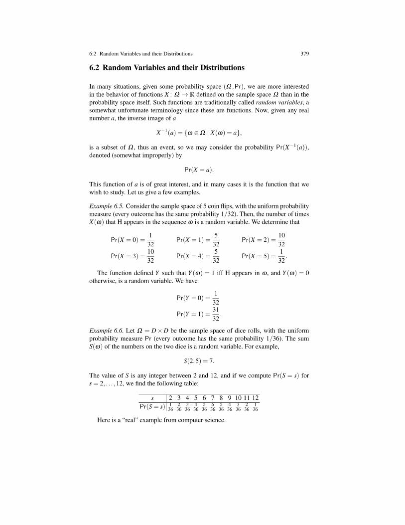
6.2 Random Variables and their Distributions 379
6.2 Random Variables and their Distributions
In many situations, given some probability space (Ω ,Pr), we are more interestedin the behavior of functions X : Ω → R defined on the sample space Ω than in theprobability space itself. Such functions are traditionally called random variables, asomewhat unfortunate terminology since these are functions. Now, given any realnumber a, the inverse image of a
X−1(a) = ω ∈Ω | X(ω) = a,
is a subset of Ω , thus an event, so we may consider the probability Pr(X−1(a)),denoted (somewhat improperly) by
Pr(X = a).
This function of a is of great interest, and in many cases it is the function that wewish to study. Let us give a few examples.
Example 6.5. Consider the sample space of 5 coin flips, with the uniform probabilitymeasure (every outcome has the same probability 1/32). Then, the number of timesX(ω) that H appears in the sequence ω is a random variable. We determine that
Pr(X = 0) =1
32Pr(X = 1) =
532
Pr(X = 2) =1032
Pr(X = 3) =1032
Pr(X = 4) =5
32Pr(X = 5) =
132
.
The function defined Y such that Y (ω) = 1 iff H appears in ω , and Y (ω) = 0otherwise, is a random variable. We have
Pr(Y = 0) =132
Pr(Y = 1) =3132
.
Example 6.6. Let Ω = D×D be the sample space of dice rolls, with the uniformprobability measure Pr (every outcome has the same probability 1/36). The sumS(ω) of the numbers on the two dice is a random variable. For example,
S(2,5) = 7.
The value of S is any integer between 2 and 12, and if we compute Pr(S = s) fors = 2, . . . ,12, we find the following table:
s 2 3 4 5 6 7 8 9 10 11 12Pr(S = s) 1
36236
336
436
536
636
536
436
336
236
136
Here is a “real” example from computer science.
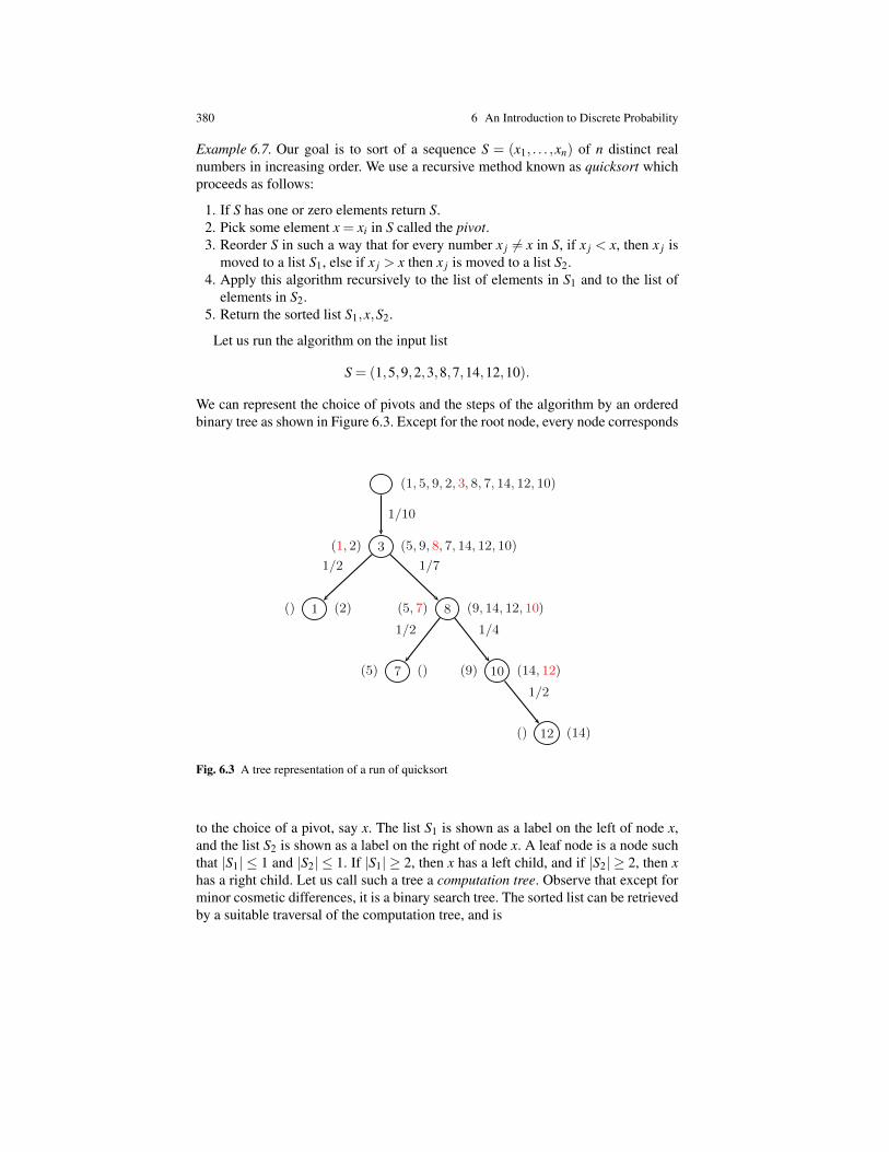
380 6 An Introduction to Discrete Probability
Example 6.7. Our goal is to sort of a sequence S = (x1, . . . ,xn) of n distinct realnumbers in increasing order. We use a recursive method known as quicksort whichproceeds as follows:
1. If S has one or zero elements return S.2. Pick some element x = xi in S called the pivot.3. Reorder S in such a way that for every number x j 6= x in S, if x j < x, then x j is
moved to a list S1, else if x j > x then x j is moved to a list S2.4. Apply this algorithm recursively to the list of elements in S1 and to the list of
elements in S2.5. Return the sorted list S1,x,S2.
Let us run the algorithm on the input list
S = (1,5,9,2,3,8,7,14,12,10).
We can represent the choice of pivots and the steps of the algorithm by an orderedbinary tree as shown in Figure 6.3. Except for the root node, every node corresponds
3
1 8
7 10
12
1/10
1/2 1/7
1/2 1/4
1/2
(1, 5, 9, 2, 3, 8, 7, 14, 12, 10)
(5, 9, 8, 7, 14, 12, 10)(1, 2)
(2)() (9, 14, 12, 10)(5, 7)
()(5) (14, 12)(9)
(14)()
Fig. 6.3 A tree representation of a run of quicksort
to the choice of a pivot, say x. The list S1 is shown as a label on the left of node x,and the list S2 is shown as a label on the right of node x. A leaf node is a node suchthat |S1| ≤ 1 and |S2| ≤ 1. If |S1| ≥ 2, then x has a left child, and if |S2| ≥ 2, then xhas a right child. Let us call such a tree a computation tree. Observe that except forminor cosmetic differences, it is a binary search tree. The sorted list can be retrievedby a suitable traversal of the computation tree, and is

6.2 Random Variables and their Distributions 381
(1,2,3,5,7,8,9,10,12,14).
If you run this algorithm on a few more examples, you will realize that the choiceof pivots greatly influences how many comparisons are needed. If the pivot is chosenat each step so that the size of the lists S1 and S2 is roughly the same, then the numberof comparisons is small compared to n, in fact O(n lnn). On the other hand, with apoor choice of pivot, the number of comparisons can be as bad as n(n−1)/2.
In order to have a good “average performance,” one can randomize this algorithmby assuming that each pivot is chosen at random. What this means is that wheneverit is necessary to pick a pivot from some list Y , some procedure is called and thisprocedure returns some element chosen at random from Y . How exactly this done isan interesting topic in itself but we will not go into this. Let us just say that the pivotcan be produced by a random number generator, or by spinning a wheel containingthe numbers in Y on it, or by rolling a dice with as many faces as the numbers in Y .What we do assume is that the probability distribution that a number is chosen froma list Y is uniform, and that successive choices of pivots are independent. How dowe model this as a probability space?
Here is a way to do it. Use the computation trees defined above! Simply addto every edge the probability that one of the element of the corresponding list, sayY , was chosen uniformly, namely 1/|Y |. So, given an input list S of length n, thesample space Ω is the set of all computation trees T with root label S. We assigna probability to the trees T in Ω as follows: If n = 0,1, then there is a single treeand its probability is 1. If n≥ 2, for every leaf of T , multiply the probabilities alongthe path from the root to that leaf and then add up the probabilities assigned tothese leaves. This is Pr(T ). We leave it as an exercise to prove that the sum of theprobabilities of all the trees in Ω is equal to 1.
A random variable of great interest on (Ω ,Pr) is the number X of comparisonsperformed by the algorithm. To analyse the average running time of this algorithm,it is necessary to determine when the first (or the last) element of a sequence
Y = (yi, . . . ,y j)
is chosen as a pivot. To carry out the analysis further requires the notion of expecta-tion that has not yet been defined. See Example 6.23 for a complete analysis.
Let us now give an official definition of a random variable.
Definition 6.4. Given a (finite) discrete probability space (Ω ,Pr), a random vari-able is any function X : Ω → R. For any real number a ∈ R, we define Pr(X = a)as the probability
Pr(X = a) = Pr(X−1(a)) = Pr(ω ∈Ω | X(ω) = a),
and Pr(X ≤ a) as the probability
Pr(X ≤ a) = Pr(X−1((−∞,a])) = Pr(ω ∈Ω | X(ω)≤ a).

382 6 An Introduction to Discrete Probability
The function f : R→ [0,1] given by
f (a) = Pr(X = a), a ∈ R
is the probability mass function of X , and the function F : R→ [0,1] given by
F(a) = Pr(X ≤ a), a ∈ R
is the cumulative distribution function of X .
The term probability mass function is abbreviated as p.m.f , and cumulative dis-tribution function is abbreviated as c.d.f . It is unfortunate and confusing that boththe probability mass function and the cumulative distribution function are often ab-breviated as distribution function.
The probability mass function f for the sum S of the numbers on two dice fromExample 6.6 is shown in Figure 6.4, and the corresponding cumulative distributionfunction F is shown in Figure 6.5.
Fig. 6.4 The probability mass function for the sum of the numbers on two dice
If Ω is finite, then f only takes finitely many nonzero values; it is very discontin-uous! The c.d.f F of S shown in Figure 6.5 has jumps (steps). Observe that the sizeof the jump at every value a is equal to f (a) = Pr(S = a).
The cumulative distribution function F has the following properties:
1. We havelim
x 7→−∞F(x) = 0, lim
x 7→∞F(x) = 1.
2. It is monotonic nondecreasing, which means that if a≤ b, then F(a)≤ F(b).3. It is piecewise constant with jumps, but it is right-continuous, which means that
limh>0,h7→0 F(a+h) = F(a).
For any a ∈ R, because F is nondecreasing, we can define F(a−) by
F(a−) = limh↓0
F(a−h) = limh>0,h7→0
F(a−h).
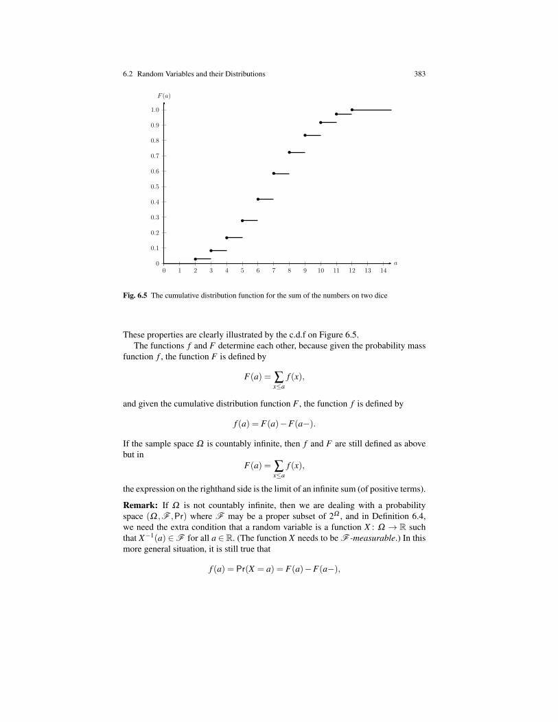
6.2 Random Variables and their Distributions 383
0
0.1
0.2
0.3
0.4
0.5
0.6
0.7
0.8
0.9
1.0
0 1 2 3 4 5 6 7 8 9 10 11 12 13 14a
F (a)
Fig. 6.5 The cumulative distribution function for the sum of the numbers on two dice
These properties are clearly illustrated by the c.d.f on Figure 6.5.The functions f and F determine each other, because given the probability mass
function f , the function F is defined by
F(a) = ∑x≤a
f (x),
and given the cumulative distribution function F , the function f is defined by
f (a) = F(a)−F(a−).
If the sample space Ω is countably infinite, then f and F are still defined as abovebut in
F(a) = ∑x≤a
f (x),
the expression on the righthand side is the limit of an infinite sum (of positive terms).
Remark: If Ω is not countably infinite, then we are dealing with a probabilityspace (Ω ,F ,Pr) where F may be a proper subset of 2Ω , and in Definition 6.4,we need the extra condition that a random variable is a function X : Ω → R suchthat X−1(a) ∈F for all a ∈R. (The function X needs to be F -measurable.) In thismore general situation, it is still true that
f (a) = Pr(X = a) = F(a)−F(a−),
384 6 An Introduction to Discrete Probability
but F cannot generally be recovered from f . If the c.d.f F of a random variable Xcan be expressed as
F(x) =∫ x
−∞
f (y)dy,
for some nonnegative (Lebesgue) integrable function f , then we say that F and Xare absolutely continuous (please, don’t ask me what type of integral!). The functionf is called a probability density function of X (for short, p.d.f ).
In this case, F is continuous, but more is true. The function F is uniformly con-tinuous, and it is differentiable almost everywhere, which means that the set of inputvalues for which it is not differentiable is a set of (Lebesgue) measure zero. Further-more, F ′ = f almost everywhere.
Random variables whose distributions can be expressed as above in terms of adensity function are often called continuous random variables. In contrast with thediscrete case, if X is a continuous random variable, then
Pr(X = x) = 0 for all x ∈ R.
As a consequence, some of the definitions given in the discrete case in terms of theprobabilities Pr(X = x), for example Definition 6.7, become trivial. These defini-tions need to be modifed; replacing Pr(X = x) by Pr(X ≤ x) usually works.
In the general case where the cdf F of a random variable X has discontinuities,we say that X is a discrete random variable if X(ω) 6= 0 for at most countably manyω ∈ Ω . Equivalently, the image of X is finite or countably infinite. In this case, themass function of X is well defined, and it can be viewed as a discrete version of adensity function.
In the discrete setting where the sample space Ω is finite, it is usually moreconvenient to use the probability mass function f , and to abuse language and call itthe distribution of X .
Example 6.8. Suppose we flip a coin n times, but this time, the coin is not necessarilyfair, so the probability of landing heads is p and the probability of landing tailsis 1− p. The sample space Ω is the set of strings of length n over the alphabetH,T. Assume that the coin flips are independent, so that the probability of anevent ω ∈ Ω is obtained by replacing H by p and T by 1− p in ω . Then, let X bethe random variable defined such that X(ω) is the number of heads in ω . For any iwith 0≤ i≤ n, since there are
(ni
)subsets with i elements, and since the probability
of a sequence ω with i occurrences of H is pi(1− p)n−i, we see that the distributionof X (mass function) is given by
f (i) =(
ni
)pi(1− p)n−i, i = 0, . . . ,n,
and 0 otherwise. This is an example of a binomial distribution.
Example 6.9. As in Example 6.8, assume that we flip a biased coin, where the prob-ability of landing heads is p and the probability of landing tails is 1− p. However,

6.2 Random Variables and their Distributions 385
this time, we flip our coin any finite number of times (not a fixed number), and weare interested in the event that heads first turns up. The sample space Ω is the infiniteset of strings over the alphabet H,T of the form
Ω = H,TH,TTH, . . . , TnH, . . . ,.
Assume that the coin flips are independent, so that the probability of an event ω ∈Ω
is obtained by replacing H by p and T by 1− p in ω . Then, let X be the randomvariable defined such that X(ω) = n iff |ω| = n, else 0. In other words, X is thenumber of trials until we obtain a success. Then, it is clear that
f (n) = (1− p)n−1 p, n≥ 1.
and 0 otherwise. This is an example of a geometric distribution.
The process in which we flip a coin n times is an example of a process in whichwe perform n independent trials, each of which results in success of failure (suchtrials that result exactly two outcomes, success or failure, are known as Bernoulli tri-als). Such processes are named after Jacob Bernoulli, a very significant contributorto probability theory after Fermat and Pascal.
Fig. 6.6 Jacob (Jacques) Bernoulli (1654–1705)
Example 6.10. Let us go back to Example 6.8, but assume that n is large and thatthe probability p of success is small, which means that we can write np = λ with λ
of “moderate” size. Let us show that we can approximate the distribution f of X inan interesting way. Indeed, for every nonnegative integer i, we can write
f (i) =(
ni
)pi(1− p)n−i
=n!
i!(n− i)!
(λ
n
)i (1− λ
n
)n−i
=n(n−1) · · ·(n− i+1)
niλ i
i!
(1− λ
n
)n(1− λ
n
)−i
.
Now, for n large and λ moderate, we have
386 6 An Introduction to Discrete Probability(1− λ
n
)n
≈ e−λ
(1− λ
n
)−i
≈ 1n(n−1) · · ·(n− i+1)
ni ≈ 1,
so we obtain
f (i)≈ e−λ λ i
i!, i ∈ N.
The above is called a Poisson distribution with parameter λ . It is named after theFrench mathematician Simeon Denis Poisson.
Fig. 6.7 Simeon Denis Poisson (1781–1840)
It turns out that quite a few random variables occurring in real life obey thePoisson probability law (by this, we mean that their distribution is the Poisson dis-tribution). Here are a few examples:
1. The number of misprints on a page (or a group of pages) in a book.2. The number of people in a community whose age is over a hundred.3. The number of wrong telephone numbers that are dialed in a day.4. The number of customers entering a post office each day.5. The number of vacancies occurring in a year in the federal judicial system.
As we will see later on, the Poisson distribution has some nice mathematicalproperties, and the so-called Poisson paradigm which consists in approximating thedistribution of some process by a Poisson distribution is quite useful.
6.3 Conditional Probability and Independence
In general, the occurrence of some event B changes the probability that anotherevent A occurs. It is then natural to consider the probability denoted Pr(A | B) thatif an event B occurs, then A occurs. As in logic, if B does not occur not much can besaid, so we assume that Pr(B) 6= 0.
Definition 6.5. Given a discrete probability space (Ω ,Pr), for any two events A andB, if Pr(B) 6= 0, then we define the conditional probability Pr(A | B) that A occursgiven that B occurs as
6.3 Conditional Probability and Independence 387
Pr(A | B) = Pr(A∩B)Pr(B)
.
Example 6.11. Suppose we roll two fair dice. What is the conditional probabilitythat the sum of the numbers on the dice exceeds 6, given that the first shows 3? Tosolve this problem, let
B = (3, j) | 1≤ j ≤ 6be the event that the first dice shows 3, and
A = (i, j) | i+ j ≥ 7,1≤ i, j ≤ 6
be the event that the total exceeds 6. We have
A∩B = (3,4),(3,5),(3,6),
so we get
Pr(A | B) = Pr(A∩B)Pr(B)
=336
/6
36=
12.
The next example is perhaps a little more surprising.
Example 6.12. A family has two children. What is the probability that both are boys,given at least one is a boy?
There are four possible combinations of sexes, so the sample space is
Ω = GG,GB,BG,BB,
and we assume a uniform probability measure (each outcome has probability 1/4).Introduce the events
B = GB,BG,BBof having at least one boy, and
A = BBof having two boys. We get
A∩B = BB,and so
Pr(A | B) = Pr(A∩B)Pr(B)
=14
/34=
13.
Contrary to the popular belief that Pr(A | B) = 1/2, it is actually equal to 1/3. Now,consider the question: what is the probability that both are boys given that the firstchild is a boy? The answer to this question is indeed 1/2.
The next example is known as the “Monty Hall Problem,” a standard example ofevery introduction to probability theory.
Example 6.13. On the old television game Let’s make a deal, a contestant is pre-sented with a choice of three (closed) doors. Behind exactly one door is a terrific
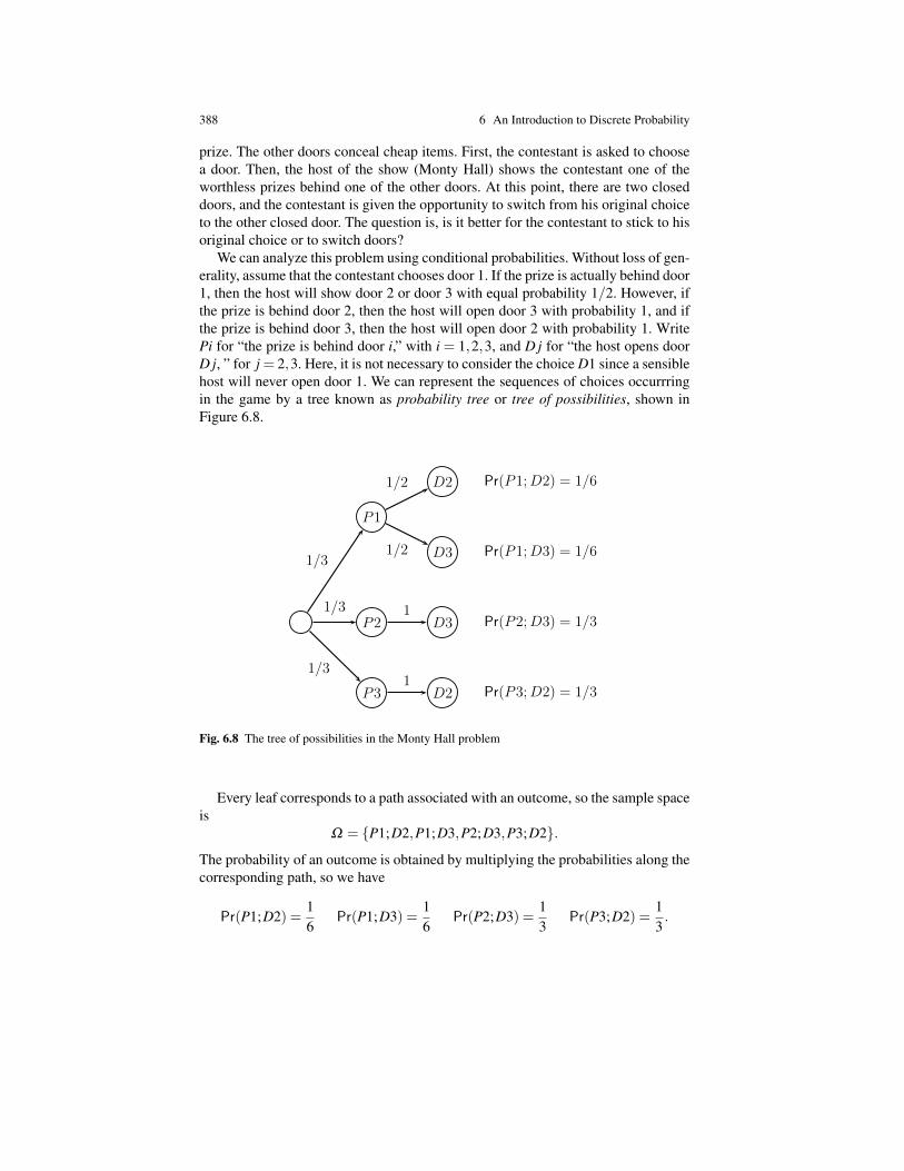
388 6 An Introduction to Discrete Probability
prize. The other doors conceal cheap items. First, the contestant is asked to choosea door. Then, the host of the show (Monty Hall) shows the contestant one of theworthless prizes behind one of the other doors. At this point, there are two closeddoors, and the contestant is given the opportunity to switch from his original choiceto the other closed door. The question is, is it better for the contestant to stick to hisoriginal choice or to switch doors?
We can analyze this problem using conditional probabilities. Without loss of gen-erality, assume that the contestant chooses door 1. If the prize is actually behind door1, then the host will show door 2 or door 3 with equal probability 1/2. However, ifthe prize is behind door 2, then the host will open door 3 with probability 1, and ifthe prize is behind door 3, then the host will open door 2 with probability 1. WritePi for “the prize is behind door i,” with i = 1,2,3, and D j for “the host opens doorD j, ” for j = 2,3. Here, it is not necessary to consider the choice D1 since a sensiblehost will never open door 1. We can represent the sequences of choices occurrringin the game by a tree known as probability tree or tree of possibilities, shown inFigure 6.8.
P1
P2
P3
D2
D3
D3
D2
1/3
1/3
1/3
1/2
1/2
1
1
Pr(P1; D2) = 1/6
Pr(P1; D3) = 1/6
Pr(P2; D3) = 1/3
Pr(P3; D2) = 1/3
Fig. 6.8 The tree of possibilities in the Monty Hall problem
Every leaf corresponds to a path associated with an outcome, so the sample spaceis
Ω = P1;D2,P1;D3,P2;D3,P3;D2.The probability of an outcome is obtained by multiplying the probabilities along thecorresponding path, so we have
Pr(P1;D2) =16
Pr(P1;D3) =16
Pr(P2;D3) =13
Pr(P3;D2) =13.
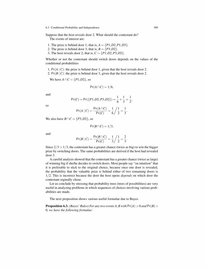
6.3 Conditional Probability and Independence 389
Suppose that the host reveals door 2. What should the contestant do?The events of interest are:
1. The prize is behind door 1; that is, A = P1;D2,P1;D3.2. The prize is behind door 3; that is, B = P3;D2.3. The host reveals door 2; that is, C = P1;D2,P3;D2.
Whether or not the contestant should switch doors depends on the values of theconditional probabilities
1. Pr(A |C): the prize is behind door 1, given that the host reveals door 2.2. Pr(B |C): the prize is behind door 3, given that the host reveals door 2.
We have A∩C = P1;D2, so
Pr(A∩C) = 1/6,
andPr(C) = Pr(P1;D2,P3;D2) = 1
6+
13=
12,
so
Pr(A |C) =Pr(A∩C)
Pr(C)=
16
/12=
13.
We also have B∩C = P3;D2, so
Pr(B∩C) = 1/3,
and
Pr(B |C) =Pr(B∩C)
Pr(C)=
13
/12=
23.
Since 2/3 > 1/3, the contestant has a greater chance (twice as big) to win the biggerprize by switching doors. The same probabilities are derived if the host had revealeddoor 3.
A careful analysis showed that the contestant has a greater chance (twice as large)of winning big if she/he decides to switch doors. Most people say “on intuition” thatit is preferable to stick to the original choice, because once one door is revealed,the probability that the valuable prize is behind either of two remaining doors is1/2. This is incorrect because the door the host opens depends on which door thecontestant orginally chose.
Let us conclude by stressing that probability trees (trees of possibilities) are veryuseful in analyzing problems in which sequences of choices involving various prob-abilities are made.
The next proposition shows various useful formulae due to Bayes.
Proposition 6.3. (Bayes’ Rules) For any two events A,B with Pr(A)> 0 and Pr(B)>0, we have the following formulae:
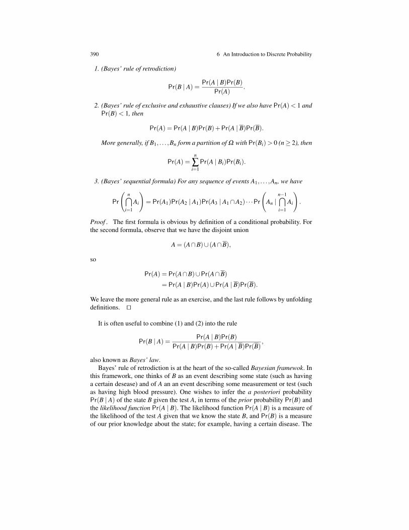
390 6 An Introduction to Discrete Probability
1. (Bayes’ rule of retrodiction)
Pr(B | A) = Pr(A | B)Pr(B)Pr(A)
.
2. (Bayes’ rule of exclusive and exhaustive clauses) If we also have Pr(A)< 1 andPr(B)< 1, then
Pr(A) = Pr(A | B)Pr(B)+Pr(A | B)Pr(B).
More generally, if B1, . . . ,Bn form a partition of Ω with Pr(Bi)> 0 (n≥ 2), then
Pr(A) =n
∑i=1
Pr(A | Bi)Pr(Bi).
3. (Bayes’ sequential formula) For any sequence of events A1, . . . ,An, we have
Pr
(n⋂
i=1
Ai
)= Pr(A1)Pr(A2 | A1)Pr(A3 | A1∩A2) · · ·Pr
(An |
n−1⋂i=1
Ai
).
Proof . The first formula is obvious by definition of a conditional probability. Forthe second formula, observe that we have the disjoint union
A = (A∩B)∪ (A∩B),
so
Pr(A) = Pr(A∩B)∪Pr(A∩B)
= Pr(A | B)Pr(A)∪Pr(A | B)Pr(B).
We leave the more general rule as an exercise, and the last rule follows by unfoldingdefinitions. ut
It is often useful to combine (1) and (2) into the rule
Pr(B | A) = Pr(A | B)Pr(B)Pr(A | B)Pr(B)+Pr(A | B)Pr(B) ,
also known as Bayes’ law.Bayes’ rule of retrodiction is at the heart of the so-called Bayesian framewok. In
this framework, one thinks of B as an event describing some state (such as havinga certain desease) and of A an an event describing some measurement or test (suchas having high blood pressure). One wishes to infer the a posteriori probabilityPr(B | A) of the state B given the test A, in terms of the prior probability Pr(B) andthe likelihood function Pr(A | B). The likelihood function Pr(A | B) is a measure ofthe likelihood of the test A given that we know the state B, and Pr(B) is a measureof our prior knowledge about the state; for example, having a certain disease. The
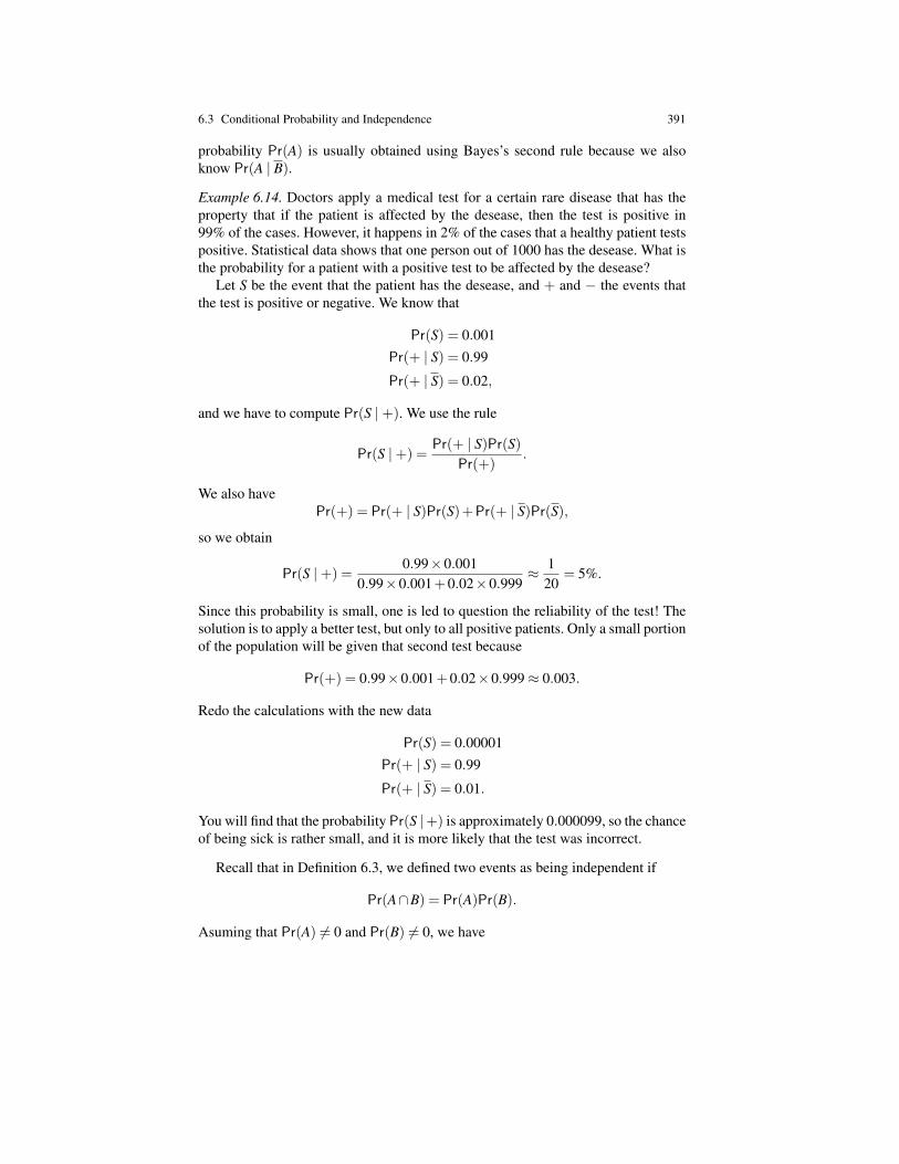
6.3 Conditional Probability and Independence 391
probability Pr(A) is usually obtained using Bayes’s second rule because we alsoknow Pr(A | B).
Example 6.14. Doctors apply a medical test for a certain rare disease that has theproperty that if the patient is affected by the desease, then the test is positive in99% of the cases. However, it happens in 2% of the cases that a healthy patient testspositive. Statistical data shows that one person out of 1000 has the desease. What isthe probability for a patient with a positive test to be affected by the desease?
Let S be the event that the patient has the desease, and + and − the events thatthe test is positive or negative. We know that
Pr(S) = 0.001Pr(+ | S) = 0.99
Pr(+ | S) = 0.02,
and we have to compute Pr(S |+). We use the rule
Pr(S |+) =Pr(+ | S)Pr(S)
Pr(+).
We also havePr(+) = Pr(+ | S)Pr(S)+Pr(+ | S)Pr(S),
so we obtain
Pr(S |+) =0.99×0.001
0.99×0.001+0.02×0.999≈ 1
20= 5%.
Since this probability is small, one is led to question the reliability of the test! Thesolution is to apply a better test, but only to all positive patients. Only a small portionof the population will be given that second test because
Pr(+) = 0.99×0.001+0.02×0.999≈ 0.003.
Redo the calculations with the new data
Pr(S) = 0.00001Pr(+ | S) = 0.99
Pr(+ | S) = 0.01.
You will find that the probability Pr(S |+) is approximately 0.000099, so the chanceof being sick is rather small, and it is more likely that the test was incorrect.
Recall that in Definition 6.3, we defined two events as being independent if
Pr(A∩B) = Pr(A)Pr(B).
Asuming that Pr(A) 6= 0 and Pr(B) 6= 0, we have

392 6 An Introduction to Discrete Probability
Pr(A∩B) = Pr(A | B)Pr(B) = Pr(B | A)Pr(A),
so we get the following proposition.
Proposition 6.4. For any two events A,B such that Pr(A) 6= 0 and Pr(B) 6= 0, thefollowing statements are equivalent:
1. Pr(A∩B) = Pr(A)Pr(B); that is, A and B are independent.2. Pr(B | A) = Pr(B).3. Pr(A | B) = Pr(A).
Remark: For a fixed event B with Pr(B) > 0, the function A 7→ Pr(A | B) satisfiesthe axioms of a probability measure stated in Definition 6.2. This is shown in Ross[11] (Section 3.5), among other references.
The examples where we flip a coin n times or roll two dice n times are examplesof indendent repeated trials. They suggest the following definition.
Definition 6.6. Given two discrete probability spaces (Ω1,Pr1) and (Ω2,Pr2), wedefine their product space as the probability space (Ω1×Ω2,Pr), where Pr is givenby
Pr(ω1,ω2) = Pr1(ω1)Pr2(Ω2), ω1 ∈Ω1,ω2 ∈Ω2.
There is an obvious generalization for n discrete probability spaces. In particular, forany discrete probability space (Ω ,Pr) and any integer n≥ 1, we define the productspace (Ω n,Pr), with
Pr(ω1, . . . ,ωn) = Pr(ω1) · · ·Pr(ωn), ωi ∈Ω , i = 1, . . . ,n.
The fact that the probability measure on the product space is defined as a prod-uct of the probability measures of its components captures the independence of thetrials.
Remark: The product of two probability spaces (Ω1,F1,Pr1) and (Ω2,F2,Pr2)can also be defined, but F1×F2 is not a σ -algebra in general, so some seriouswork needs to be done.
The notion of independence also applies to random variables. Given two randomvariables X and Y on the same (discrete) probability space, it is useful to considertheir joint distribution (really joint mass function) fX ,Y given by
fX ,Y (a,b) = Pr(X = a and Y = b) = Pr(ω ∈Ω | (X(ω) = a)∧ (Y (ω) = b)),
for any two reals a,b ∈ R.
Definition 6.7. Two random variables X and Y defined on the same discrete proba-bility space are independent if
Pr(X = a and Y = b) = Pr(X = a)Pr(Y = b), for all a,b ∈ R.
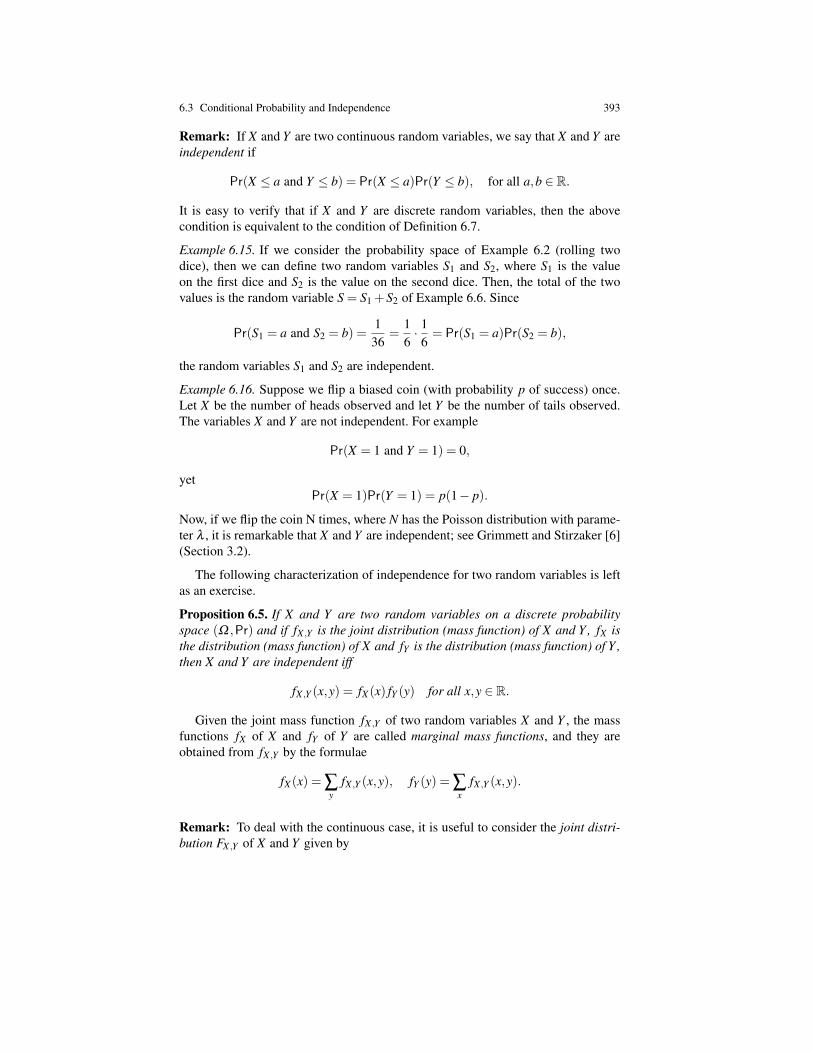
6.3 Conditional Probability and Independence 393
Remark: If X and Y are two continuous random variables, we say that X and Y areindependent if
Pr(X ≤ a and Y ≤ b) = Pr(X ≤ a)Pr(Y ≤ b), for all a,b ∈ R.
It is easy to verify that if X and Y are discrete random variables, then the abovecondition is equivalent to the condition of Definition 6.7.
Example 6.15. If we consider the probability space of Example 6.2 (rolling twodice), then we can define two random variables S1 and S2, where S1 is the valueon the first dice and S2 is the value on the second dice. Then, the total of the twovalues is the random variable S = S1 +S2 of Example 6.6. Since
Pr(S1 = a and S2 = b) =136
=16· 1
6= Pr(S1 = a)Pr(S2 = b),
the random variables S1 and S2 are independent.
Example 6.16. Suppose we flip a biased coin (with probability p of success) once.Let X be the number of heads observed and let Y be the number of tails observed.The variables X and Y are not independent. For example
Pr(X = 1 and Y = 1) = 0,
yetPr(X = 1)Pr(Y = 1) = p(1− p).
Now, if we flip the coin N times, where N has the Poisson distribution with parame-ter λ , it is remarkable that X and Y are independent; see Grimmett and Stirzaker [6](Section 3.2).
The following characterization of independence for two random variables is leftas an exercise.
Proposition 6.5. If X and Y are two random variables on a discrete probabilityspace (Ω ,Pr) and if fX ,Y is the joint distribution (mass function) of X and Y , fX isthe distribution (mass function) of X and fY is the distribution (mass function) of Y ,then X and Y are independent iff
fX ,Y (x,y) = fX (x) fY (y) for all x,y ∈ R.
Given the joint mass function fX ,Y of two random variables X and Y , the massfunctions fX of X and fY of Y are called marginal mass functions, and they areobtained from fX ,Y by the formulae
fX (x) = ∑y
fX ,Y (x,y), fY (y) = ∑x
fX ,Y (x,y).
Remark: To deal with the continuous case, it is useful to consider the joint distri-bution FX ,Y of X and Y given by
394 6 An Introduction to Discrete Probability
FX ,Y (a,b) = Pr(X ≤ a and Y ≤ b) = Pr(ω ∈Ω | (X(ω)≤ a)∧ (Y (ω)≤ b)),
for any two reals a,b ∈ R. We say that X and Y are jointly continuous with jointdensity function fX ,Y if
FX ,Y (x,y) =∫ x
−∞
∫ y
−∞
fX ,Y (u,v)dudv, for all x,y ∈ R
for some nonnegative integrable function fX ,Y . The marginal density functions fXof X and fY of Y are defined by
fX (x) =∫
∞
−∞
fX ,Y (x,y)dy, fY (y) =∫
∞
−∞
fX ,Y (x,y)dx.
They correspond to the marginal distribution functions FX of X and FY of Y givenby
FX (x) = Pr(X ≤ x) = FX ,Y (x,∞), FY (y) = Pr(Y ≤ y) = FX ,Y (∞,y).
Then, it can be shown that X and Y are independent iff
FX ,Y (x,y) = FX (x)FY (y) for all x,y ∈ R,
which, for continuous variables, is equivalent to
fX ,Y (x,y) = fX (x) fY (y) for all x,y ∈ R.
We now turn to one of the most important concepts about random variables, theirmean (or expectation).
6.4 Expectation of a Random Variable
In order to understand the behavior of a random variable, we may want to look atits “average” value. But the notion of average in ambiguous, as there are differentkinds of averages that we might want to consider. Among these, we have
1. the mean: the sum of the values divided by the number of values.2. the median: the middle value (numerically).3. the mode: the value that occurs most often.
For example, the mean of the sequence (3,1,4,1,5) is 2.8; the median is 3, and themode is 1.
Given a random variable X , if we consider a sequence of values X(ω1),X(ω2), . . .,X(ωn), each value X(ω j) = a j has a certain probability Pr(X = a j) of occurringwhich may differ depending on j, so the usual mean
6.4 Expectation of a Random Variable 395
X(ω1)+X(ω2)+ · · ·+X(ωn)
n=
a1 + · · ·+an
n
may not capture well the “average” of the random variable X . A better solution is touse a weighted average, where the weights are probabilities. If we write a j = X(ω j),we can define the mean of X as the quantity
a1Pr(X = a1)+a2Pr(X = a2)+ · · ·+anPr(X = an).
Definition 6.8. Given a discrete probability space (Ω ,Pr), for any random variableX , the mean value or expected value or expectation1 of X is the number E(X) definedas
E(X) = ∑x∈X(Ω)
x ·Pr(X = x) = ∑x| f (x)>0
x f (x),
where X(Ω) denotes the image of the function X and where f is the probabilitymass function of X . Because Ω is finite, we can also write
E(X) = ∑ω∈Ω
X(ω)Pr(ω).
In this setting, the median of X is defined as the set of elements x ∈ X(Ω) suchthat
Pr(X ≤ x)≥ 12
and Pr(X ≥ x)≥ 12.
Remark: If Ω is countably infinite, then the expectation E(X), if it exists, is givenby
E(X) = ∑x| f (x)>0
x f (x),
provided that the above sum converges absolutely (that is, the partial sums of abso-lute values converge). If we have a probability space (X ,F ,Pr) with Ω uncountableand if X is absolutely continuous so that it has a density function f , then the expec-tation of X is given by the integral
E(X) =∫ +∞
−∞
x f (x)dx.
It is even possible to define the expectation of a random variable that is not neces-sarily absolutely continuous using its cumulative density function F as
E(X) =∫ +∞
−∞
xdF(x),
where the above integral is the Lebesgue–Stieljes integal, but this is way beyond thescope of this book.
1 It is amusing that in French, the word for expectation is esperance mathematique. There is hopefor mathematics!

396 6 An Introduction to Discrete Probability
Observe that if X is a constant random variable (that is, X(ω) = c for all ω ∈Ω
for some constant c), then
E(X) = ∑ω∈Ω
X(ω)Pr(ω) = c ∑ω∈Ω
Pr(ω) = cPr(Ω) = c,
since Pr(Ω) = 1. The mean of a constant random variable is itself (as it should be!).
Example 6.17. Consider the sum S of the values on the dice from Example 6.6. Theexpectation of S is
E(S) = 2 · 136
+3 · 236
+ · · ·+6 · 536
+7 · 636
+8 · 536
+ · · ·+12 · 136
= 7.
Example 6.18. Suppose we flip a biased coin once (with probability p of landingheads). If X is the random variable given by X(H) = 1 and X(T) = 0, the expectationof X is
E(X) = 1 ·Pr(X = 1)+0 ·Pr(X = 0) = 1 ·P+0 · (1− p) = p.
Example 6.19. Consider the binomial distribution of Example 6.8, where the ran-dom variable X counts the number of tails (success) in a sequence of n trials. Let uscompute E(X). Since the mass function is given by
f (i) =(
ni
)pi(1− p)n−i, i = 0, . . . ,n,
we have
E(X) =n
∑i=0
i f (i) =n
∑i=0
i(
ni
)pi(1− p)n−i.
We use a trick from analysis to compute this sum. Recall from the binomial theoremthat
(1+ x)n =n
∑i=0
(ni
)xi.
If we take derivatives on both sides, we get
n(1+ x)n−1 =n
∑i=0
i(
ni
)xi−1,
and by multiplying both sides by x,
nx(1+ x)n−1 =n
∑i=0
i(
ni
)xi.
Now, if we set x = p/q, since p+q = 1, we get

6.4 Expectation of a Random Variable 397
n
∑i=0
i(
ni
)pi(1− p)n−i = np,
and soE(X) = np.
It should be observed that the expectation of a random variable may be infinite.For example, if X is a random variable whose probability mass function f is givenby
f (k) =1
k(k+1), k = 1,2, . . . ,
then ∑k∈N−0 f (k) = 1, since
∞
∑k=1
1k(k+1)
=∞
∑k=1
(1k− 1
k+1
)= lim
k 7→∞
(1− 1
k+1
)= 1,
butE(X) = ∑
k∈N−0k f (k) = ∑
k∈N−0
1k+1
= ∞.
A crucial property of expectation that often allows simplifications in computingthe expectation of a random variable is its linearity.
Proposition 6.6. (Linearity of Expectation) Given two random variables on a dis-crete probability space, for any real number λ , we have
E(X +Y ) = E(X)+E(Y )
E(λX) = λE(X).
Proof . We have
E(X +Y ) = ∑z
z ·Pr(X +Y = z)
= ∑x
∑y(x+ y) ·Pr(X = x and Y = y)
= ∑x
∑y
x ·Pr(X = x and Y = y)+∑x
∑y
y ·Pr(X = x and Y = y)
= ∑x
∑y
x ·Pr(X = x and Y = y)+∑y
∑x
y ·Pr(X = x and Y = y)
= ∑x
x∑yPr(X = x and Y = y)+∑
yy∑
xPr(X = x and Y = y).
Now, the events Ax = x | X = x form a partition of Ω , which implies that
∑yPr(X = x and Y = y) = Pr(X = x).
Similarly the events By = y | Y = y form a partition of Ω , which implies that
398 6 An Introduction to Discrete Probability
∑xPr(X = x and Y = y) = Pr(Y = y).
By substitution, we obtain
E(X +Y ) = ∑x
x ·Pr(X = x)+∑y
y ·Pr(Y = y),
proving that E(X +Y ) = E(X)+E(Y ). When Ω is countably infinite, we can per-mute the indices x and y due to absolute convergence.
For the second equation, if λ 6= 0, we have
E(λX) = ∑x
x ·Pr(λX = x)
= λ ∑x
xλ·Pr(X = x/λ )
= λ ∑x
y ·Pr(X = y)
= λE(X).
as claimed. If λ = 0, the equation is trivial. ut
By a trivial induction, we obtain that for any finite number of random variablesX1, . . . ,Xn, we have
E
( n
∑I=1
Xi
)=
n
∑I=1
E(Xi).
It is also important to realize that the above equation holds even if the Xi are notindependent.
Here is an example showing how the linearity of expectation can simplify calcu-lations. Let us go back to Example 6.19. Define n random variables X1, . . . ,Xn suchthat Xi(ω) = 1 iff the ith flip yields heads, otherwise Xi(ω) = 0. Clearly, the numberX of heads in the sequence is
X = X1 + · · ·+Xn.
However, we saw in Example 6.18 that E(Xi) = p, and since
E(X) = E(X1)+ · · ·+E(Xn),
we getE(X) = np.
The above example suggests the definition of indicator function, which turns outto be quite handy.
Definition 6.9. Given a discrete probability space with sample space Ω , for anyevent A, the indicator function (or indicator variable) of A is the random variable IAdefined such that
6.4 Expectation of a Random Variable 399
IA(ω) =1 if ω ∈ A
0 if ω /∈ A.
The main property of the indicator function IA is that its expectation is equal tothe probabilty Pr(A) of the event A. Indeed,
E(IA) = ∑ω∈Ω
IA(ω)Pr(ω)
= ∑ω∈A
Pr(ω)
= Pr(A).
This fact with the linearity of expectation is often used to compute the expectationof a random variable, by expressing it as a sum of indicator variables. We will seehow this method is used to compute the expectation of the number of comparisons inquicksort. But first, we use this method to find the expected number of fixed pointsof a random permutation.
Example 6.20. For any integer n ≥ 1, let Ω be the set of all n! permutations of1, . . . ,n, and give Ω the uniform probabilty measure; that is, for every permutationπ , let
Pr(π) =1n!.
We say that these are random permutations. A fixed point of a permutation π is anyinteger k such that π(k) = k. Let X be the random variable such that X(π) is thenumber of fixed points of the permutation π . Let us find the expectation of X . To dothis, for every k, let Xk be the random variable defined so that Xk(π) = 1 iff π(k) = k,and 0 otherwise. Clearly,
X = X1 + · · ·+Xn,
and sinceE(X) = E(X1)+ · · ·+E(Xn),
we just have to compute E(Xk). But, Xk is an indicator variable, so
E(Xk) = Pr(Xk = 1).
Now, there are (n−1)! permutations that leave k fixed, so Pr(X = 1) = 1/n. There-fore,
E(X) = E(X1)+ · · ·+E(Xn) = n · 1n= 1.
On average, a random permutation has one fixed point.
If X is a random variable on a discrete probability space Ω (possibly countablyinfinite), for any function g : R→ R, the composition g X is a random variabledefined by
(gX)(ω) = g(X(ω)), ω ∈Ω .
This random variable is usually denoted by g(X).

400 6 An Introduction to Discrete Probability
Given two random variables X and Y , if ϕ and ψ are two functions, we leave itas an exercise to prove that if X and Y are independent, then so are ϕ(X) and ψ(Y ).
Altough computing its mass function in terms of the mass function f of X can bevery difficult, there is a nice way to compute its expectation.
Proposition 6.7. If X is a random variable on a discrete probability space Ω , forany function g : R→ R, the expectation E(g(X)) of g(X) (if it exists) is given by
E(g(X)) = ∑x
g(x) f (x),
where f is the mass function of X.
Proof . We have
E(g(X)) = ∑y
y ·Pr(gX = y)
= ∑y
y ·Pr(ω ∈Ω | g(X(ω)) = y)
= ∑y
y∑xPr(ω ∈Ω | g(x) = y, X(ω) = x)
= ∑y
∑x,g(x)=y
y ·Pr(ω ∈Ω , | X(ω) = x)
= ∑y
∑x,g(x)=y
g(x) ·Pr(X = x)
= ∑x
g(x) ·Pr(X = x)
= ∑x
g(x) f (x),
as claimed.
The cases g(X) = Xk, g(X) = zX , and g(X) = etX (for some given reals z and t)are of particular interest.
Given two random variables X and Y on a discrete probability space Ω , for anyfunction g : R×R→ R, then g(X ,Y ) is a random variable and it is easy to showthat E(g(X ,Y )) (if it exists) is given by
E(g(X ,Y )) = ∑x,y
g(x,y) fX ,Y (x,y),
where fX ,Y is the joint mass function of X and Y .
Example 6.21. Consider the random variable X of Example 6.19 counting the num-ber of heads in a sequence of coin flips of length n, but this time, let us try to computeE(Xk), for k ≥ 2. We have
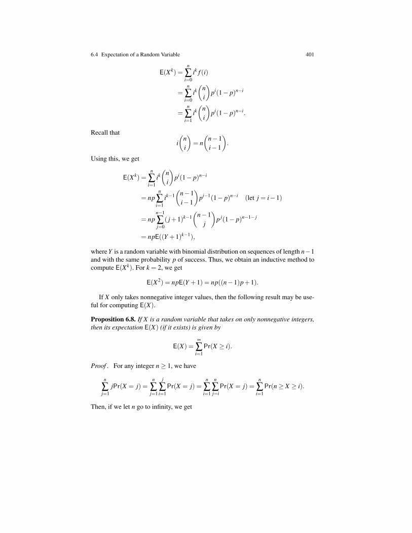
6.4 Expectation of a Random Variable 401
E(Xk) =n
∑i=0
ik f (i)
=n
∑i=0
ik(
ni
)pi(1− p)n−i
=n
∑i=1
ik(
ni
)pi(1− p)n−i.
Recall that
i(
ni
)= n(
n−1i−1
).
Using this, we get
E(Xk) =n
∑i=1
ik(
ni
)pi(1− p)n−i
= npn
∑i=1
ik−1(
n−1i−1
)pi−1(1− p)n−i (let j = i−1)
= npn−1
∑j=0
( j+1)k−1(
n−1j
)p j(1− p)n−1− j
= npE((Y +1)k−1),
where Y is a random variable with binomial distribution on sequences of length n−1and with the same probability p of success. Thus, we obtain an inductive method tocompute E(Xk). For k = 2, we get
E(X2) = npE(Y +1) = np((n−1)p+1).
If X only takes nonnegative integer values, then the following result may be use-ful for computing E(X).
Proposition 6.8. If X is a random variable that takes on only nonnegative integers,then its expectation E(X) (if it exists) is given by
E(X) =∞
∑i=1
Pr(X ≥ i).
Proof . For any integer n≥ 1, we have
n
∑j=1
jPr(X = j) =n
∑j=1
j
∑i=1
Pr(X = j) =n
∑i=1
n
∑j=i
Pr(X = j) =n
∑i=1
Pr(n≥ X ≥ i).
Then, if we let n go to infinity, we get
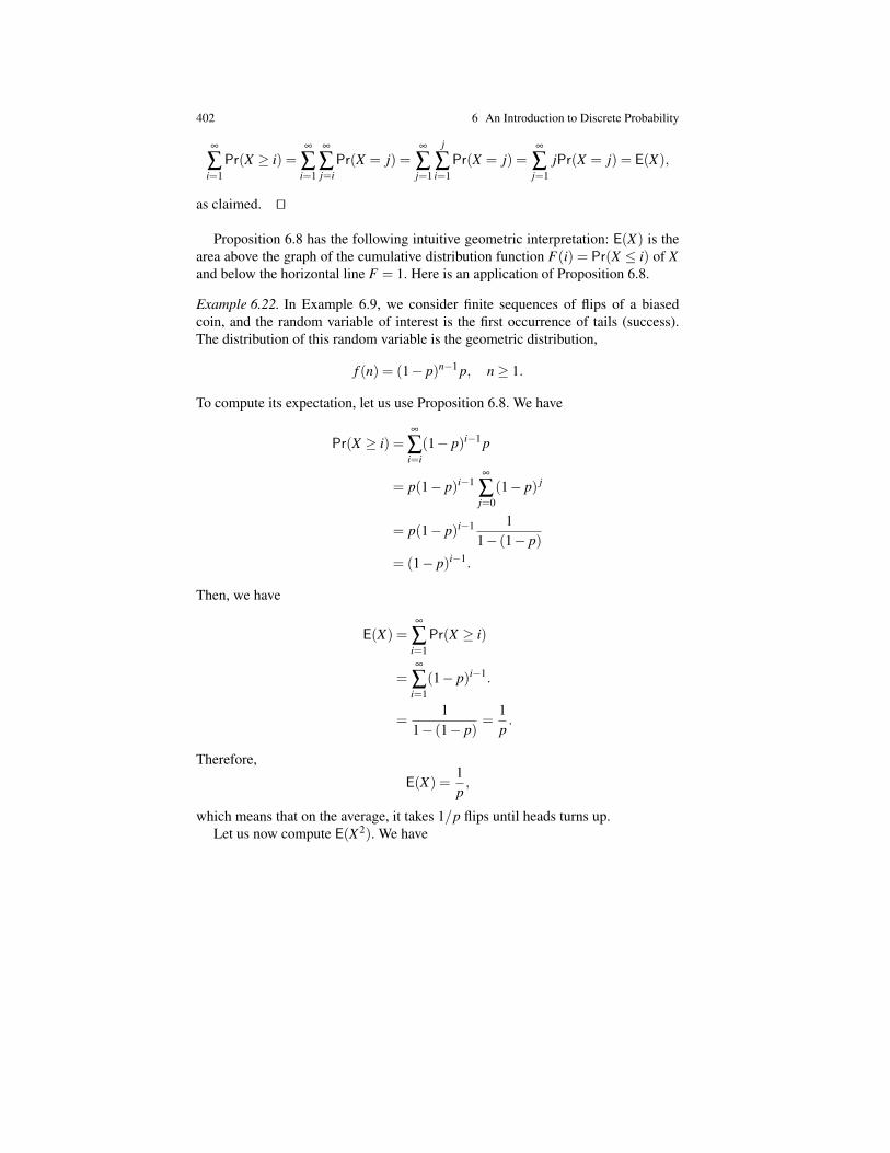
402 6 An Introduction to Discrete Probability
∞
∑i=1
Pr(X ≥ i) =∞
∑i=1
∞
∑j=i
Pr(X = j) =∞
∑j=1
j
∑i=1
Pr(X = j) =∞
∑j=1
jPr(X = j) = E(X),
as claimed. ut
Proposition 6.8 has the following intuitive geometric interpretation: E(X) is thearea above the graph of the cumulative distribution function F(i) = Pr(X ≤ i) of Xand below the horizontal line F = 1. Here is an application of Proposition 6.8.
Example 6.22. In Example 6.9, we consider finite sequences of flips of a biasedcoin, and the random variable of interest is the first occurrence of tails (success).The distribution of this random variable is the geometric distribution,
f (n) = (1− p)n−1 p, n≥ 1.
To compute its expectation, let us use Proposition 6.8. We have
Pr(X ≥ i) =∞
∑i=i
(1− p)i−1 p
= p(1− p)i−1∞
∑j=0
(1− p) j
= p(1− p)i−1 11− (1− p)
= (1− p)i−1.
Then, we have
E(X) =∞
∑i=1
Pr(X ≥ i)
=∞
∑i=1
(1− p)i−1.
=1
1− (1− p)=
1p.
Therefore,
E(X) =1p,
which means that on the average, it takes 1/p flips until heads turns up.Let us now compute E(X2). We have
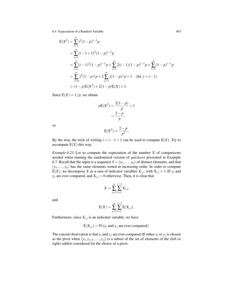
6.4 Expectation of a Random Variable 403
E(X2) =∞
∑i=1
i2(1− p)i−1 p
=∞
∑i=1
(i−1+1)2(1− p)i−1 p
=∞
∑i=1
(i−1)2(1− p)i−1 p+∞
∑i=1
2(i−1)(1− p)i−1 p+∞
∑i=1
(1− p)i−1 p
=∞
∑j=0
j2(1− p) j p+2∞
∑j=1
j(1− p) j p+1 (let j = i−1)
= (1− p)E(X2)+2(1− p)E(X)+1.
Since E(X) = 1/p, we obtain
pE(X2) =2(1− p)
p+1
=2− p
p,
soE(X2) =
2− pp2 .
By the way, the trick of writing i = i− 1+ 1 can be used to compute E(X). Try torecompute E(X) this way.
Example 6.23. Let us compute the expectation of the number X of comparisonsneeded when running the randomized version of quicksort presented in Example6.7. Recall that the input is a sequence S = (x1, . . . ,xn) of distinct elements, and that(y1, . . . ,yn) has the same elements sorted in increasing order. In order to computeE(X), we decompose X as a sum of indicator variables Xi, j, with Xi, j = 1 iff yi andy j are ever compared, and Xi, j = 0 otherwise. Then, it is clear that
X =n
∑j=2
j−1
∑i=1
Xi, j,
and
E(X) =n
∑j=2
j−1
∑i=1
E(Xi, j).
Furthermore, since Xi, j is an indicator variable, we have
E(Xi, j) = Pr(yi and y j are ever compared).
The crucial observation is that yi and y j are ever compared iff either yi or y j is chosenas the pivot when yi,yi+1, . . . ,y j is a subset of the set of elements of the (left orright) sublist considered for the choice of a pivot.
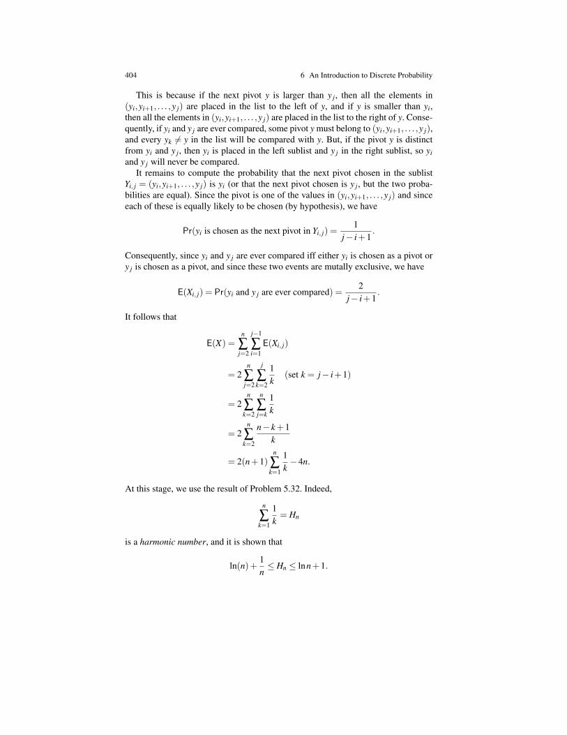
404 6 An Introduction to Discrete Probability
This is because if the next pivot y is larger than y j, then all the elements in(yi,yi+1, . . . ,y j) are placed in the list to the left of y, and if y is smaller than yi,then all the elements in (yi,yi+1, . . . ,y j) are placed in the list to the right of y. Conse-quently, if yi and y j are ever compared, some pivot y must belong to (yi,yi+1, . . . ,y j),and every yk 6= y in the list will be compared with y. But, if the pivot y is distinctfrom yi and y j, then yi is placed in the left sublist and y j in the right sublist, so yiand y j will never be compared.
It remains to compute the probability that the next pivot chosen in the sublistYi, j = (yi,yi+1, . . . ,y j) is yi (or that the next pivot chosen is y j, but the two proba-bilities are equal). Since the pivot is one of the values in (yi,yi+1, . . . ,y j) and sinceeach of these is equally likely to be chosen (by hypothesis), we have
Pr(yi is chosen as the next pivot in Yi, j) =1
j− i+1.
Consequently, since yi and y j are ever compared iff either yi is chosen as a pivot ory j is chosen as a pivot, and since these two events are mutally exclusive, we have
E(Xi, j) = Pr(yi and y j are ever compared) =2
j− i+1.
It follows that
E(X) =n
∑j=2
j−1
∑i=1
E(Xi, j)
= 2n
∑j=2
j
∑k=2
1k
(set k = j− i+1)
= 2n
∑k=2
n
∑j=k
1k
= 2n
∑k=2
n− k+1k
= 2(n+1)n
∑k=1
1k−4n.
At this stage, we use the result of Problem 5.32. Indeed,
n
∑k=1
1k= Hn
is a harmonic number, and it is shown that
ln(n)+1n≤ Hn ≤ lnn+1.

6.4 Expectation of a Random Variable 405
Therefore, Hn = lnn+Θ(1), which shows that
E(X) = 2n ln+Θ(n).
Therefore, the expected number of comparisons made by the randomized version ofquicksort is 2n lnn+Θ(n).
Example 6.24. If X is a random variable with Poisson distribution with parameter λ
(see Example 6.10), let us show that its expectation is
E(X) = λ .
Recall that a Poisson distribution is given by
f (i) = e−λ λ i
i!, i ∈ N,
so we have
E(X) =∞
∑i=0
ie−λ λ i
i!
= λe−λ∞
∑i=1
λ i−1
(i−1)!
= λe−λ∞
∑j=0
λ j
j!(let j = i−1)
= λe−λ eλ = λ ,
as claimed. This is consistent with the fact that the expectation of a random variablewith a binomial distribution is np, under the Poisson approximation where λ = np.We leave it as an exercise to prove that
E(X2) = λ (λ +1).
Alhough in general E(XY ) 6= E(X)E(Y ), this is true for independent random vari-ables.
Proposition 6.9. If two random variables X and Y on the same discrete probabilityspace are independent, then
E(XY ) = E(X)E(Y ).
Proof . We have

406 6 An Introduction to Discrete Probability
E(XY ) = ∑ω∈Ω
X(ω)Y (ω)Pr(ω)
= ∑x
∑y
xy ·Pr(X = x and Y = y)
= ∑x
∑y
xy ·Pr(X = x)Pr(Y = y)
=
(∑x
x ·Pr(X = x))(
∑y
y ·Pr(Y = y))
= E(X)E(Y ),
as claimed. Note that the independence of X and Y was used in going from line 2 toline 3. ut
In Example 6.15 (rolling two dice), we defined the random variables S1 and S2,where S1 is the value on the first dice and S2 is the value on the second dice. Wealso showed that S1 and S2 are independent. If we consider the random variableP = S1S2, then we have
E(P) = E(S1)E(S2) =72· 7
2=
494,
since E(S1) = E(S2) = 7/2, as we easily determine since all probabilities are equalto 1/6. On the other hand, S and P are not independent (check it).
6.5 Variance, Standard Deviation, Chebyshev’s Inequality
The mean (expectation) E(X) of a random variable X gives some useful informationabout it, but it does not say how X is spread. Another quantity, the variance Var(X),measure the spread of the distribution by finding the “average” of the square differ-ence (X−E(X))2, namely
Var(X) = E(X−E(X))2.
Note that computing E(X−E(X)) yields no information since
E(X−E(X)) = E(X)−E(E(X)) = E(X)−E(X) = 0.
Definition 6.10. Given a discrete probability space (Ω ,Pr), for any random variableX , the variance Var(X) of X (if it exists) is defined as
Var(X) = E(X−E(X))2.
The expectation E(X) of a random variable X is often denoted by µ . The varianceis also denoted V(X), for instance, in Graham, Knuth and Patashnik [5]).
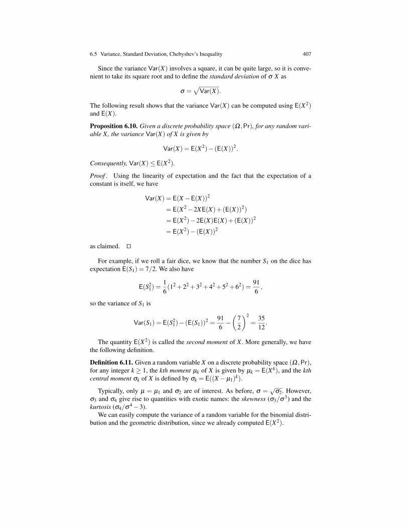
6.5 Variance, Standard Deviation, Chebyshev’s Inequality 407
Since the variance Var(X) involves a square, it can be quite large, so it is conve-nient to take its square root and to define the standard deviation of σ X as
σ =√Var(X).
The following result shows that the variance Var(X) can be computed using E(X2)and E(X).
Proposition 6.10. Given a discrete probability space (Ω ,Pr), for any random vari-able X, the variance Var(X) of X is given by
Var(X) = E(X2)− (E(X))2.
Consequently, Var(X)≤ E(X2).
Proof . Using the linearity of expectation and the fact that the expectation of aconstant is itself, we have
Var(X) = E(X−E(X))2
= E(X2−2XE(X)+(E(X))2)
= E(X2)−2E(X)E(X)+(E(X))2
= E(X2)− (E(X))2
as claimed. ut
For example, if we roll a fair dice, we know that the number S1 on the dice hasexpectation E(S1) = 7/2. We also have
E(S21) =
16(12 +22 +32 +42 +52 +62) =
916,
so the variance of S1 is
Var(S1) = E(S21)− (E(S1))
2 =916−(
72
)2
=3512
.
The quantity E(X2) is called the second moment of X . More generally, we havethe following definition.
Definition 6.11. Given a random variable X on a discrete probability space (Ω ,Pr),for any integer k ≥ 1, the kth moment µk of X is given by µk = E(Xk), and the kthcentral moment σk of X is defined by σk = E((X−µ1)
k).
Typically, only µ = µ1 and σ2 are of interest. As before, σ =√
σ2. However,σ3 and σ4 give rise to quantities with exotic names: the skewness (σ3/σ3) and thekurtosis (σ4/σ4−3).
We can easily compute the variance of a random variable for the binomial distri-bution and the geometric distribution, since we already computed E(X2).
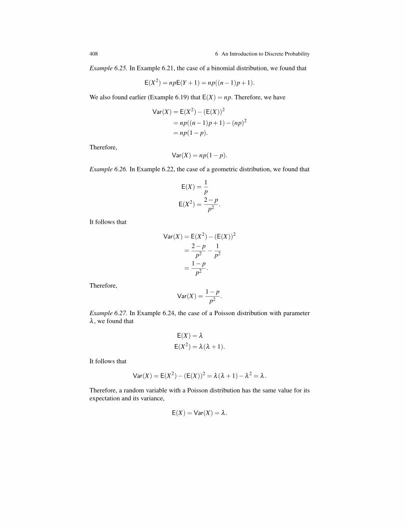
408 6 An Introduction to Discrete Probability
Example 6.25. In Example 6.21, the case of a binomial distribution, we found that
E(X2) = npE(Y +1) = np((n−1)p+1).
We also found earlier (Example 6.19) that E(X) = np. Therefore, we have
Var(X) = E(X2)− (E(X))2
= np((n−1)p+1)− (np)2
= np(1− p).
Therefore,Var(X) = np(1− p).
Example 6.26. In Example 6.22, the case of a geometric distribution, we found that
E(X) =1p
E(X2) =2− p
p2 .
It follows that
Var(X) = E(X2)− (E(X))2
=2− p
p2 −1p2
=1− p
p2 .
Therefore,
Var(X) =1− p
p2 .
Example 6.27. In Example 6.24, the case of a Poisson distribution with parameterλ , we found that
E(X) = λ
E(X2) = λ (λ +1).
It follows that
Var(X) = E(X2)− (E(X))2 = λ (λ +1)−λ2 = λ .
Therefore, a random variable with a Poisson distribution has the same value for itsexpectation and its variance,
E(X) = Var(X) = λ .
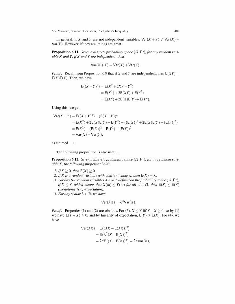
6.5 Variance, Standard Deviation, Chebyshev’s Inequality 409
In general, if X and Y are not independent variables, Var(X +Y ) 6= Var(X) +Var(Y ). However, if they are, things are great!
Proposition 6.11. Given a discrete probability space (Ω ,Pr), for any random vari-able X and Y , if X and Y are independent, then
Var(X +Y ) = Var(X)+Var(Y ).
Proof . Recall from Proposition 6.9 that if X and Y are independent, then E(XY ) =E(X)E(Y ). Then, we have
E((X +Y )2) = E(X2 +2XY +Y 2)
= E(X2)+2E(XY )+E(Y 2)
= E(X2)+2E(X)E(Y )+E(Y 2).
Using this, we get
Var(X +Y ) = E((X +Y )2)− (E(X +Y ))2
= E(X2)+2E(X)E(Y )+E(Y 2)− ((E(X))2 +2E(X)E(Y )+(E(Y ))2)
= E(X2)− (E(X))2 +E(Y 2)− (E(Y ))2
= Var(X)+Var(Y ),
as claimed. ut
The following proposition is also useful.
Proposition 6.12. Given a discrete probability space (Ω ,Pr), for any random vari-able X, the following properties hold:
1. If X ≥ 0, then E(X)≥ 0.2. If X is a random variable with constant value λ , then E(X) = λ .3. For any two random variables X and Y defined on the probablity space (Ω ,Pr),
if X ≤ Y , which means that X(ω) ≤ Y (ω) for all ω ∈ Ω , then E(X) ≤ E(Y )(monotonicity of expectation).
4. For any scalar λ ∈ R, we have
Var(λX) = λ2Var(X).
Proof . Properties (1) and (2) are obvious. For (3), X ≤ Y iff Y −X ≥ 0, so by (1)we have E(Y −X) ≥ 0, and by linearity of expectation, E(Y ) ≥ E(X). For (4), wehave
Var(λX) = E((λX−E(λX))2)
= E(λ
2(X−E(X))2)= λ
2E((X−E(X))2)= λ
2Var(X),

410 6 An Introduction to Discrete Probability
as claimed. ut
Property (4) shows that unlike expectation, the variance is not linear (althoughfor independent random variables, Var(X +Y ) = Var(X)+Var(Y ). This also holdsin the more general case of uncorrelated random variables; see Proposition 6.13below).
As an application of Proposition 6.11, if we consider the event of rolling twodice, since we showed that the random variables S1 and S2 are independent, we cancompute the variance of their sum S = S1 +S2 and we get
Var(S) = Var(S1)+Var(S2) =3512
+3512
=356.
Recall that E(S) = 7.Here is an application of geometrically distributed random variables.
Example 6.28. Suppose there are m different types of coupons (or perhaps, the kindsof cards that kids like to collect), and that each time one obtains a coupon, it isequally likely to be any of these types. Let X denote the number of coupons oneneeds to collect in order to have at least one of each type. What is the expectedvalue E(X) of X? This problem is usually called a coupon collecting problem.
The trick is to introduce the random variables Xi, where Xi is the number ofadditional coupons needed, after i distinct types have been collected, until anothernew type is obtained, for i = 0,1, . . . ,m−1. Clearly,
X =m−1
∑i=0
Xi,
and each Xi has a geometric distribution, where each trial has probability of successpi = (m− i)/m. We know (see Example 6.22,) that
E(Xi) =1pi
=m
m− i.
Consequently,
E(X) =m−1
∑i=0
E(Xi) =m−1
∑i=0
mm− i
= mm
∑i=1
1i.
Once again, the harmonic number
Hm =m
∑k=1
1k
shows up! Since Hn = lnn+Θ(1), we obtain
E(X) = m lnm+Θ(m).

6.5 Variance, Standard Deviation, Chebyshev’s Inequality 411
For example, if m = 50, then ln50 = 3.912, and m lnm ≈ 196. If m = 100, thenln100 = 4.6052, and m lnm ≈ 461. If the coupons are expensive, one begins to seewhy the company makes money!
It turns out that using a little bit of analysis, we can compute the variance of X .This is because it is easy to check that the Xi are independent, so
Var(X) =m−1
∑i=0
Var(Xi).
From Example 6.22, we have
Var(Xi) =1− pi
p2i
=
(1− m− i
m
)/m2
(m− i)2 =mi
(m− i)2 .
It follows that
Var(X) =m−1
∑i=0
Var(Xi) = mm
∑i=1
i(m− i)2 .
To compute this sum, write
m−1
∑i=0
i(m− i)2 =
m−1
∑i=0
m(m− i)2 −
m−1
∑i=0
m− i(m− i)2
=m−1
∑i=0
m(m− i)2 −
m−1
∑i=0
1(m− i)
= mm
∑j=1
1j2 −
m
∑j=1
1j.
Now, it is well known from analysis that
limm7→∞
m
∑j=1
1j2 =
π2
6,
so we get
Var(X) =m2π2
6+Θ(m lnm).
Let us go back to the example about fixed points of random permutations (Ex-ample 6.20). We found that the expectation of the number of fixed points is µ = 1.The reader should compute the standard deviation. The difficulty is that the ran-dom variables Xk are not independent, (for every permutation π , we have Xk(π) = 1iff π(k) = k, and 0 otherwise). You will find that σ = 1. If you get stuck, look atGraham, Knuth and Patashnik [5], Chapter 8.
If X and Y are not independent, we still have
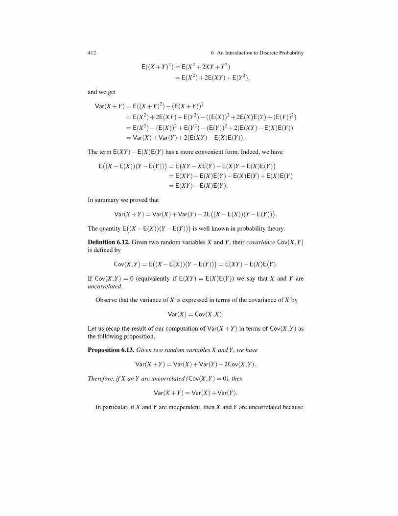
412 6 An Introduction to Discrete Probability
E((X +Y )2) = E(X2 +2XY +Y 2)
= E(X2)+2E(XY )+E(Y 2),
and we get
Var(X +Y ) = E((X +Y )2)− (E(X +Y ))2
= E(X2)+2E(XY )+E(Y 2)− ((E(X))2 +2E(X)E(Y )+(E(Y ))2)
= E(X2)− (E(X))2 +E(Y 2)− (E(Y ))2 +2(E(XY )−E(X)E(Y ))
= Var(X)+Var(Y )+2(E(XY )−E(X)E(Y )).
The term E(XY )−E(X)E(Y ) has a more convenient form. Indeed, we have
E((X−E(X))(Y −E(Y ))
)= E
(XY −XE(Y )−E(X)Y +E(X)E(Y )
)= E(XY )−E(X)E(Y )−E(X)E(Y )+E(X)E(Y )
= E(XY )−E(X)E(Y ).
In summary we proved that
Var(X +Y ) = Var(X)+Var(Y )+2E((X−E(X))(Y −E(Y ))
).
The quantity E((X−E(X))(Y −E(Y ))
)is well known in probability theory.
Definition 6.12. Given two random variables X and Y , their covariance Cov(X ,Y )is defined by
Cov(X ,Y ) = E((X−E(X))(Y −E(Y ))
)= E(XY )−E(X)E(Y ).
If Cov(X ,Y ) = 0 (equivalently if E(XY ) = E(X)E(Y )) we say that X and Y areuncorrelated.
Observe that the variance of X is expressed in terms of the covariance of X by
Var(X) = Cov(X ,X).
Let us recap the result of our computation of Var(X +Y ) in terms of Cov(X ,Y ) asthe following proposition.
Proposition 6.13. Given two random variables X and Y , we have
Var(X +Y ) = Var(X)+Var(Y )+2Cov(X ,Y ).
Therefore, if X an Y are uncorrelated (Cov(X ,Y ) = 0), then
Var(X +Y ) = Var(X)+Var(Y ).
In particular, if X and Y are independent, then X and Y are uncorrelated because
6.5 Variance, Standard Deviation, Chebyshev’s Inequality 413
Cov(X ,Y ) = E(XY )−E(X)E(Y ) = E(X)E(Y )−E(X)E(Y ) = 0.
This yields another proof of Proposition 6.11.However, beware that Cov(X ,Y ) = 0 does not necessarily imply that X and Y are
independent. For example, let X and Y be the random variables defined on −1,0,1by
Pr(X = 0) = Pr(X = 1) = Pr(X =−1) =13,
andY =
0 if X 6= 01 if X = 0 .
Since XY = 0, we have E(XY ) = 0, and since we also have E(X) = 0, we have
Cov(X ,Y ) = E(XY )−E(X)E(Y ) = 0.
However, the reader will check easily that X and Y are not independent.A better measure of independence is given by the correlation coefficient ρ(X ,Y )
of X and Y , given by
ρ(X ,Y ) =Cov(X ,Y )√
Var(X)√
Var(Y ),
provided that Var(X) 6= 0 and Var(Y ) 6= 0. It turns out that |ρ(X ,Y )| ≤ 1, which isshown using the Cauchy–Schwarz inequality.
Proposition 6.14. (Cauchy–Schwarz inequality) For any two random variables Xand Y on a discrete probability space Ω , we have
|E(XY )| ≤√
E(X2)√
E(Y 2).
Equality is achieved if and only if there exist some α,β ∈ R (not both zero) suchthat E((αX +βY )2) = 0.
Proof . This is a standard argument involving a quadratic equation. For any λ ∈ R,define the function T (λ ) by
T (λ ) = E((X +λY )2).
We get
T (λ ) = E(X2 +2λXY +λ2Y 2)
= E(X2)+2λE(XY )+λ2E(Y 2).
Since E((X+λY )2)≥ 0, we have T (λ )≥ 0 for all λ ∈R. If E(Y 2)= 0, then we musthave E(XY ) = 0, since otherwise we could choose λ so that E(X2)+2λE(XY )< 0.In this case, the inequality is trivial. If E(Y 2) > 0, then for T (λ ) to be nonnegativethe quadratic equation
414 6 An Introduction to Discrete Probability
E(X2)+2λE(XY )+λ2E(Y 2) = 0
should have at most one real root, which is equivalent to the well-known condition
4(E(XY ))2−4E(X2)E(Y 2)≤ 0,
which is equivalent to
|E(XY )| ≤√
E(X2)√
E(Y 2),
as claimed. If (E(XY ))2 = E(X2)E(Y 2), then either E(Y 2) = 0, and then with α =0,β = 1, we have E((αX +βY )2) = 0, or E(Y 2) > 0, in which case the quadraticequation
E(X2)+2λE(XY )+λ2E(Y 2) = 0
has a unique real root λ0, so we have E((X +λ0Y )2) = 0.Conversely, if E((αX +βY )2) = 0 for some α,β ∈ R, then either E(Y 2) = 0, in
which case we showed that we also have E(XY ) = 0, or the quadratic equation hassome real root, so we must have (E(XY ))2−E(X2)E(Y 2) = 0. In both cases, wehave (E(XY ))2 = E(X2)E(Y 2). ut
It can be shown that for any random variable Z, if E(Z2) = 0, then Pr(Z = 0) =1; see Grimmett and Stirzaker [6] (Chapter 3, Problem 3.11.2). In fact, this is aconsequence of Proposition 6.2 and Chebyshev’s Inequality (see below), as shownin Ross [11] (Section 8.2, Proposition 2.3). It follows that if equality is achieved inthe Cauchy–Schwarz inequality, then there are some reals α,β (not both zero) suchthat Pr(αX +βY = 0) = 1; in other words, X and Y are dependent with probability1. If we apply the Cauchy-Schwarz inequality to the random variables X−E(X) andY −E(Y ), we obtain the following result.
Proposition 6.15. For any two random variables X and Y on a discrete probabilityspace, we have
|ρ(X ,Y )| ≤ 1,
with equality iff there are some real numbers α,β ,γ (with α,β not both zero) suchthat Pr(αX +βY = γ) = 1.
As emphasized by Graham, Knuth and Patashnik [5], the variance plays a keyrole in an inquality due to Chebyshev (published in 1867) that tells us that a randomvariable will rarely be far from its mean E(X) if its variance Var(X) is small.
Proposition 6.16. (Chebyshev’s Inequality) If X is any random variable, for everyα > 0, we have
Pr((X−E(X))2 ≥ α
)≤ Var(X)
α
Proof . We follow Knuth. We have
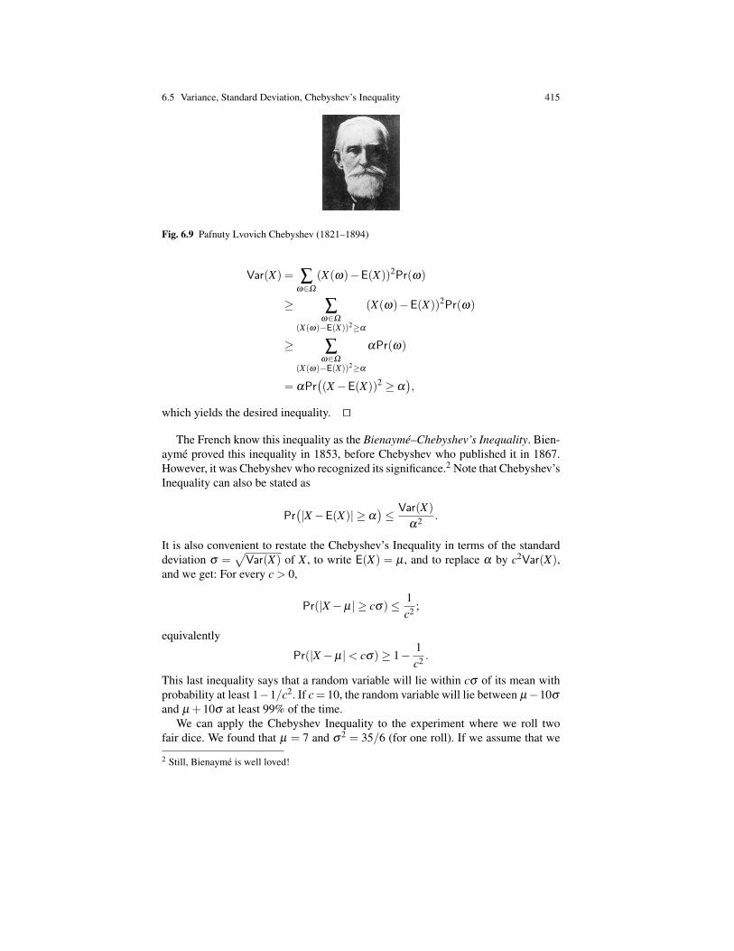
6.5 Variance, Standard Deviation, Chebyshev’s Inequality 415
Fig. 6.9 Pafnuty Lvovich Chebyshev (1821–1894)
Var(X) = ∑ω∈Ω
(X(ω)−E(X))2Pr(ω)
≥ ∑ω∈Ω
(X(ω)−E(X))2≥α
(X(ω)−E(X))2Pr(ω)
≥ ∑ω∈Ω
(X(ω)−E(X))2≥α
αPr(ω)
= αPr((X−E(X))2 ≥ α
),
which yields the desired inequality. ut
The French know this inequality as the Bienayme–Chebyshev’s Inequality. Bien-ayme proved this inequality in 1853, before Chebyshev who published it in 1867.However, it was Chebyshev who recognized its significance.2 Note that Chebyshev’sInequality can also be stated as
Pr(|X−E(X)| ≥ α
)≤ Var(X)
α2 .
It is also convenient to restate the Chebyshev’s Inequality in terms of the standarddeviation σ =
√Var(X) of X , to write E(X) = µ , and to replace α by c2Var(X),
and we get: For every c > 0,
Pr(|X−µ| ≥ cσ)≤ 1c2 ;
equivalently
Pr(|X−µ|< cσ)≥ 1− 1c2 .
This last inequality says that a random variable will lie within cσ of its mean withprobability at least 1−1/c2. If c= 10, the random variable will lie between µ−10σ
and µ +10σ at least 99% of the time.We can apply the Chebyshev Inequality to the experiment where we roll two
fair dice. We found that µ = 7 and σ2 = 35/6 (for one roll). If we assume that we
2 Still, Bienayme is well loved!

416 6 An Introduction to Discrete Probability
perform n independent trials, then the total value of the n rolls has expecation 7nand the variance if 35n/6. It follows that the sum will be between
7n−10
√35n
6and 7n+10
√35n
6
at least 99% of the time. If n = 106 (a million rolls), then the total value will bebetween 6.976 million and 7.024 million more than 99% of the time.
Another interesting consequence of the Chebyshev’s Inequality is this. Supposewe have a random variable X on some discrete probability space (Ω ,Pr). For any n,we can form the product space (Ω n,Pr) as explained in Definition 6.6, with
Pr(ω1, . . . ,ωn) = Pr(ω1) · · ·Pr(ωn), ωi ∈Ω , i = 1, . . . ,n.
Then, we define the random variable Xk on the product space by
Xk(ω1, . . . ,ωn) = X(ωk).
It is easy to see that the Xk are independent. Consider the random variable
S = X1 + · · ·+Xn.
We can think of S as taking n independent “samples” from Ω and adding them to-gether. By our previous discussion, S has mean nµ and standard deviation σ
√n,
where µ is the mean of X and σ is its standard deviation. The Chebyshev’s Inequal-ity implies that the average
X1 + · · ·+Xn
n
will lie between σ −10σ/√
n and σ +10σ/√
n at least 99% of the time. This im-plies that if we choose n large enough, then the average of n samples will almostalways be very near the expected value µ = E(X).
This concludes our elementary introduction to discrete probability. The readershould now be well prepared to move on to Grimmett and Stirzaker [6] or Venkatesh[14]. Among the references listed at the end of this chapter, let us mention the clas-sical volumes by Feller [3, 4], and Shiryaev [13].
The next three sections are devoted to more advanced topics and are optional.
6.6 Limit Theorems; A Glimpse
The behavior of the average sum of n independent samples described at the end ofSection 6.5 is an example of a weak law of large numbers. A precise formulationof such a result is shown below. A version of this result was first shown by JacobBernoulli and was published by his nephew Nicholas in 1713. Bernoulli did not have
6.6 Limit Theorems; A Glimpse 417
Chebyshev’s Inequality at this disposal (since Chebyshev Inequality was proved in1867), and he had to resort to a very ingenious proof.
Fig. 6.10 Jacob (Jacques) Bernoulli (1654–1705)
Theorem 6.1. (Weak Law of Large Numbers (“Bernoulli’s Theorem”)) Let X1,X2,. . . ,Xn, . . . be a sequence of random variables. Assume that they are independent,that they all have the same distribution, and let µ be their common mean and σ2 betheir common variance (we assume that both exist). Then, for every ε > 0,
limn7→∞
Pr
(∣∣∣∣X1 + · · ·+Xn
n−µ
∣∣∣∣≥ ε
)= 0.
Proof . As earlier,
E
(X1 + · · ·+Xn
n
)= µ
and because the Xi are independent,
Var
(X1 + · · ·+Xn
n
)=
σ2
n.
Then, we apply Chebyshev’s Inequality and we obtain
Pr
(∣∣∣∣X1 + · · ·+Xn
n−µ
∣∣∣∣≥ ε
)≤ σ2
nε2 ,
which proves the result. ut
The locution independent and identically distributed random variables is oftenused to say that some random variables are independent and have the same distribu-tion. This locution is abbreviated as i.i.d. Probability books are replete with i.i.d.’s
Another remarkable limit theorem has to do with the limit of the distribution ofthe random variable
X1 + · · ·+Xn−nµ
σ√
n,
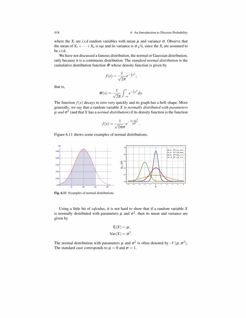
418 6 An Introduction to Discrete Probability
where the Xi are i.i.d random variables with mean µ and variance σ . Observe thatthe mean of X1 + · · ·+Xn is nµ and its variance is σ
√n, since the Xi are assumed to
be i.i.d.We have not discussed a famous distribution, the normal or Gaussian distribution,
only because it is a continuous distribution. The standard normal distribution is thecumulative distribution function Φ whose density function is given by
f (x) =1√2π
e−12 x2
;
that is,
Φ(x) =1√2π
∫ x
−∞
e−12 y2
dy.
The function f (x) decays to zero very quickly and its graph has a bell–shape. Moregenerally, we say that a random variable X is normally distributed with parametersµ and σ2 (and that X has a normal distribution) if its density function is the function
f (x) =1√
2πσe−
(x−µ)2
2σ2 .
Figure 6.11 shows some examples of normal distributions.
Fig. 6.11 Examples of normal distributions
Using a little bit of calculus, it is not hard to show that if a random variable Xis normally distributed with parameters µ and σ2, then its mean and variance aregiven by
E(X) = µ,
Var(X) = σ2.
The normal distribution with parameters µ and σ2 is often denoted by N (µ,σ2).The standard case corresponds to µ = 0 and σ = 1.
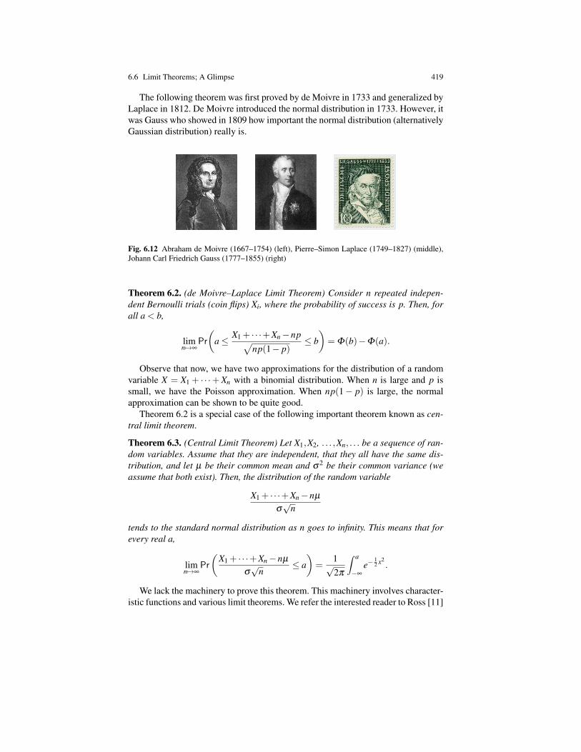
6.6 Limit Theorems; A Glimpse 419
The following theorem was first proved by de Moivre in 1733 and generalized byLaplace in 1812. De Moivre introduced the normal distribution in 1733. However, itwas Gauss who showed in 1809 how important the normal distribution (alternativelyGaussian distribution) really is.
Fig. 6.12 Abraham de Moivre (1667–1754) (left), Pierre–Simon Laplace (1749–1827) (middle),Johann Carl Friedrich Gauss (1777–1855) (right)
Theorem 6.2. (de Moivre–Laplace Limit Theorem) Consider n repeated indepen-dent Bernoulli trials (coin flips) Xi, where the probability of success is p. Then, forall a < b,
limn7→∞
Pr
(a≤ X1 + · · ·+Xn−np√
np(1− p)≤ b)= Φ(b)−Φ(a).
Observe that now, we have two approximations for the distribution of a randomvariable X = X1 + · · ·+Xn with a binomial distribution. When n is large and p issmall, we have the Poisson approximation. When np(1− p) is large, the normalapproximation can be shown to be quite good.
Theorem 6.2 is a special case of the following important theorem known as cen-tral limit theorem.
Theorem 6.3. (Central Limit Theorem) Let X1,X2, . . . ,Xn, . . . be a sequence of ran-dom variables. Assume that they are independent, that they all have the same dis-tribution, and let µ be their common mean and σ2 be their common variance (weassume that both exist). Then, the distribution of the random variable
X1 + · · ·+Xn−nµ
σ√
n
tends to the standard normal distribution as n goes to infinity. This means that forevery real a,
limn7→∞
Pr
(X1 + · · ·+Xn−nµ
σ√
n≤ a)=
1√2π
∫ a
−∞
e−12 x2
.
We lack the machinery to prove this theorem. This machinery involves character-istic functions and various limit theorems. We refer the interested reader to Ross [11]

420 6 An Introduction to Discrete Probability
(Chapter 8), Grimmett and Stirzaker [6] (Chapter 5), Venkatesh [14], and Shiryaev[13] (Chapter III).
The central limit theorem was originally stated and proved by Laplace butLaplace’s proof was not entirely rigorous. Laplace expanded a great deal of effortsin estimating sums of the form
∑k
k≤np+x√
np(1−p)
(nk
)pk(1− p)n−k
using Stirling’s formula.Reading Laplace’s classical treatise [7, 8] is an amazing experience. The intro-
duction to Volume I is 164 pages long! Among other things, it contains some inter-esting philosophical remarks about the role of probability theory, for example on thereliability of the testimony of witnesses. It is definitely worth reading. The secondpart of Volume I is devoted to the theory of generating functions, and Volume IIto probability theory proper. Laplace’s treatise was written before 1812, and eventhough the factorial notation was introduced in 1808, Laplace does not use it, whichmakes for complicated expressions. The exposition is clear, but it is difficult to readthis treatise because definitions and theorems are not clearly delineated. A versionof the central limit theorem is proved in Volume II, Chapter III; page 306 containsa key formula involving the Gaussian distribution, although Laplace does not referto it by any name (not even as normal distribution). Anybody will be struck by theelegance and beauty of the typesetting. Lyapunov gave the first rigorous proof of thecentral limit theorem around 1901.
Fig. 6.13 Pierre–Simon Laplace (1749–1827) (left), Aleksandr Mikhailovich Lyapunov (1857-1918) (right)
The following example from Ross [11] illustrates how the central limit theoremcan be used.
Example 6.29. An astronomer is interested in measuring the distance, in light-years,from his observatory to a distant star. Although the astronomer has a measuring tech-nique, he knows that, because of changing atmospheric conditions and normal error,each time a measurement is made it will not be the exact distance, but merely an ap-proximation. As a result, the astronomer plans to make a series of measurements
6.6 Limit Theorems; A Glimpse 421
and then use the average value of these measurements as his estimated value of theactual distance.
If the astronomer believes that the values of the measurements are independentand identically distributed random variables having a common mean d and a com-mon variance 4 (light-years), how many measurements need he make to be reason-ably sure that his estimated distance is accurrate to within ±0.5 light-years?
Suppose that the astronomer makes n observations, and let X1, . . . ,Xn be the nmeasurements. By the central limit theorem, the random variable
Zn =X1 + · · ·+Xn−nd
2√
n
has approximately a normal distribution. Hence,
Pr
(−1
2≤ X1 + · · ·+Xn
n≤ 1
2
)= Pr
(−1
2
√n
2≤ Zn ≤
12
√n
2
)≈Φ
(√n
4
)−Φ
(−√
n4
)= 2Φ
(√n
4
)−1.
If the astronomer wants to be 95% certain that his estimated value is accurrate towithin 0.5 light year, he should make n∗ measurements, where n∗ is given by
2Φ
(√n∗
4
)−1 = 0.95,
that is,
Φ
(√n∗
4
)= 0.975.
Using tables for the values of the function Φ , we find that√
n∗
4= 1.96,
which yieldsn∗ ≈ 61.47.
Since n should be an integer, the astronomer should make 62 observations.The above analysis relies on the assumption that the distribution of Zn is well
approximated by the normal distribution. If we are concerned about this point, wecan use Chebyshev’s inequality. If we write
Sn =X1 + · · ·+Xn−nd
2,
we have
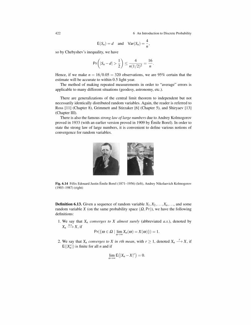
422 6 An Introduction to Discrete Probability
E(Sn) = d and Var(Sn) =4n,
so by Chebyshev’s inequality, we have
Pr
(|Sn−d|> 1
2
)≤ 4
n(1/2)2 =16n.
Hence, if we make n = 16/0.05 = 320 observations, we are 95% certain that theestimate will be accurate to within 0.5 light year.
The method of making repeated measurements in order to “average” errors isapplicable to many different situations (geodesy, astronomy, etc.).
There are generalizations of the central limit theorem to independent but notnecessarily identically distributed random variables. Again, the reader is referred toRoss [11] (Chapter 8), Grimmett and Stirzaker [6] (Chapter 5), and Shiryaev [13](Chapter III).
There is also the famous strong law of large numbers due to Andrey Kolmogorovproved in 1933 (with an earlier version proved in 1909 by Emile Borel). In order tostate the strong law of large numbers, it is convenient to define various notions ofconvergence for random variables.
Fig. 6.14 Felix Edouard Justin Emile Borel (1871–1956) (left), Andrey Nikolaevich Kolmogorov(1903–1987) (right)
Definition 6.13. Given a sequence of random variable X1,X2, . . . ,Xn, . . ., and somerandom variable X (on the same probability space (Ω ,Pr)), we have the followingdefinitions:
1. We say that Xn converges to X almost surely (abbreviated a.s.), denoted byXn
a.s.−→ X , ifPr(ω ∈Ω | lim
n7→∞Xn(ω) = X(ω)) = 1.
2. We say that Xn converges to X in rth mean, with r ≥ 1, denoted Xnr−→ X , if
E(|X rn |) is finite for all n and if
limn7→∞
E(|Xn−X |r
)= 0.
6.6 Limit Theorems; A Glimpse 423
3. We say that Xn converges to X in probability, denoted XnP−→ X , if for every
ε > 0,limn 7→∞
Pr(|Xn−X |> ε) = 0.
4. We say that Xn converges to X in distribution, denoted XnD−→ X , if
limn7→∞
Pr(Xn ≤ x) = Pr(X ≤ x),
for every x ∈ R for which F(x) = Pr(X ≤ x) is continuous.
Convergence of type (1) is also called convergence almost everywhere or conver-gence with probability 1. Almost sure convergence can be stated as the fact that theset
ω ∈Ω | Xn(ω) does not converge to X(ω)of outcomes for which convergence fails has probability 0.
It can be shown that both convergence almost surely and convergence in rthmean imply convergence in probability, which implies convergence in distribution.All converses are false. Neither convergence almost surely nor convergence in rthmean imply the other. For proofs, Interested readers should consult Grimmett andStirzaker [6] (Chapter 7) and Shiryaev [13] (Chapter III).
Observe that the convergence of the weak law of large numbers is convergencein probability, and the convergence of the central limit theorem is convergence indistribution.
The following beautiful result was obtained by Kolmogorov (1933).
Theorem 6.4. (Strong Law of Large Numbers, Kolmogorov) Let X1,X2, . . . ,Xn, . . .be a sequence of random variables. Assume that they are independent, that they allhave the same distribution, and let µ be their common mean and E(X2
1 ) be theircommon second moment (we assume that both exist). Then,
X1 + · · ·+Xn
n
converges almost surely and in mean square to µ = E(X1).
The proof is beyond the scope of this book. Interested readers should consultGrimmett and Stirzaker [6] (Chapter 7), Venkatesh [14], and Shiryaev [13] (ChapterIII). Fairly accessible proofs under the additional assumption that E(X4
1 ) exists canbe found in Bremaud [2], and Ross [11].
Actually, for almost sure convergence, the assumption that E(X21 ) exists is re-
dundant provided that E(|X1|) exists, in which case µ = E(|X1|), but the proof takessome work; see Bremaud [2] (Chapter 1, Section 8.4) and Grimmett and Stirzaker[6] (Chapter 7). There are generalizations of the strong law of large numbers wherethe independence assumption on the Xn is relaxed, but again, this is beyond thescope of this book.

424 6 An Introduction to Discrete Probability
6.7 Generating Functions; A Glimpse
If a random variables X on some discrete probability space (Ω ,Pr) takes nonnega-tive integer values, then we can define its probability generating function (for shortpgf ) GX (z) as
GX (z) = ∑k≥0
Pr(X = k)zk,
which can also be expressed as
GX (z) = ∑ω∈Ω
Pr(ω)zX(ω) = E(zX ).
ThereforeGX (z) = E(zX ).
Note thatGX (1) = ∑
ω∈Ω
Pr(ω) = 1,
so the radius of convergence of the power series GX (z) is at least 1. The nicestproperty about pgf’s is that they usually simplify the computation of the mean andvariance. For example, we have
E(X) = ∑k≥0
kPr(X = k)
= ∑k≥0
Pr(X = k) · kzk−1∣∣z=1
= G′X (1).
Similarly,
E(X2) = ∑k≥0
k2Pr(X = k)
= ∑k≥0
Pr(X = k) · (k(k−1)zk−2 + kzk−1)∣∣z=1
= G′′X (1)+G′X (1).
Therefore, we have
E(X) = G′X (1)
Var(X) = G′′X (1)+G′X (1)− (G′1(1))2.
Remark: The above results assume that G′X (1) and G′′X (1) are well defined, whichis the case if the radius of convergence of the power series GX (z) is greater than 1.If the radius of convergence of GX (z) is equal to 1 and if limz↑1 G′X (z) exists, then
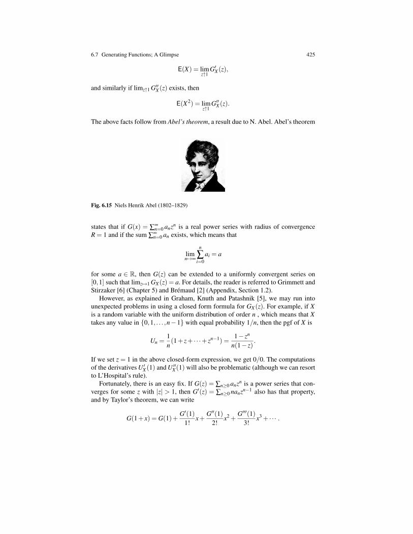
6.7 Generating Functions; A Glimpse 425
E(X) = limz↑1
G′X (z),
and similarly if limz↑1 G′′X (z) exists, then
E(X2) = limz↑1
G′′X (z).
The above facts follow from Abel’s theorem, a result due to N. Abel. Abel’s theorem
Fig. 6.15 Niels Henrik Abel (1802–1829)
states that if G(x) = ∑∞n=0 anzn is a real power series with radius of convergence
R = 1 and if the sum ∑∞n=0 an exists, which means that
limn7→∞
n
∑i=0
ai = a
for some a ∈ R, then G(z) can be extended to a uniformly convergent series on[0,1] such that limz 7→1 GX (z) = a. For details, the reader is referred to Grimmett andStirzaker [6] (Chapter 5) and Bremaud [2] (Appendix, Section 1.2).
However, as explained in Graham, Knuth and Patashnik [5], we may run intounexpected problems in using a closed form formula for GX (z). For example, if Xis a random variable with the uniform distribution of order n , which means that Xtakes any value in 0,1, . . . ,n−1 with equal probability 1/n, then the pgf of X is
Un =1n(1+ z+ · · ·+ zn−1) =
1− zn
n(1− z).
If we set z = 1 in the above closed-form expression, we get 0/0. The computationsof the derivatives U ′X (1) and U ′′X (1) will also be problematic (although we can resortto L’Hospital’s rule).
Fortunately, there is an easy fix. If G(z) = ∑n≥0 anzn is a power series that con-verges for some z with |z| > 1, then G′(z) = ∑n≥0 nanzn−1 also has that property,and by Taylor’s theorem, we can write
G(1+ x) = G(1)+G′(1)
1!x+
G′′(1)2!
x2 +G′′′(1)
3!x3 + · · · .

426 6 An Introduction to Discrete Probability
It follows that all derivatives of G(z) at z = 1 appear as coefficients when G(1+ x)is expanded in powers of x. For example, we have
Un(1+ x) =(1+ x)n−1
nx
=1n
(n1
)+
1n
(n2
)x+
1n
(n3
)x2 + · · ·+ 1
n
(nn
)xn−1.
It follows that
Un(1) = 1; U ′n(1) =n−1
2; U ′′n (1) =
(n−1)(n−2)3
;
Then, we find that the mean is given by
µ =n−1
2
and the variance by
σ2 =U ′′n (1)+U ′n(1)− (U ′n(1))
2 =n2−1
12.
Another nice fact about pgf’s is that the pdf of the sum X +Y of two indepen-dent variables X and Y is the product their pgf’s. This is because if X and Y areindependent, then
Pr(X +Y = n) =n
∑k=0
Pr(X = k and Y = n− k)
=n
∑k=0
Pr(X = k)Pr(Y = n− k),
a convolution! Therefore, if X and Y are independent, then
GX+Y (z) = GX (z)GY (z).
If we flip a biased coin where the probability of tails is p, then the pgf for thenumber of heads after one flip is
H(z) = 1− p+ pz.
If we make n independent flips, then the pgf of the number of heads is
H(z)n = (1− p+ pz)n.
This allows us to rederive the formulae for the mean and the variance. We get
µ = (Hn(z)′(1) = nH ′(1) = np,
6.7 Generating Functions; A Glimpse 427
andσ
2 = n(H ′′(1)+H ′(1)− (H ′(1))2) = n(0+ p− p2) = np(1− p).
If we flip a biased coin repeatedly until heads first turns up, we saw that therandom variable X that gives the number of trials n until the first occurrence of tailshas the geometric distribution f (n) = (1− p)n−1 p. It follows that the pgf of X is
GX (z) = pz+(1− p)pz2 + · · ·+(1− p)n−1 pzn + · · ·= pz1− (1− p)z
.
Since we are assuming that these trials are independent, the random variables thattell us that m heads are obtained has pgf
GX (z) =(
pz1− (1− p)z
)m
= pmzm∑k
(m+ k−1
k
)((1− p)z)k
= ∑j
(j−1j−m
)pm(1− p) j−mzk.
An an exercise, the reader should check that the pgf of a Poisson distribution withparameter λ is
GX (z) = eλ (z−1).
More examples of the use of pgf can be found in Graham, Knuth and Patashnik[5].
Another interesting generating function is the moment generating function MX (t).It is defined as follows: for any t ∈ R,
MX (t) = E(etX ) = ∑x
etx f (x),
where f (x) is the mass function of X . If X is a continuous random variable withdensity function f , then
MX (t) =∫
∞
−∞
etx f (x)dx.
The main problem with the moment generating function is that it is not alwaysdefined for all t ∈ R. If MX (t) converges absolutely on some open interval (−r,r)with r > 0, then its nth derivative for t = 0 is given by
M(n)(0) = ∑x
xnetx f (x)∣∣t=0 = ∑
xxn f (x) = E(Xn).
Therefore, the moments of X are all defined and given by
E(Xn) = M(n)(0).
Within the radius of convergence of MX (t), we have the Taylor expansion
428 6 An Introduction to Discrete Probability
MX (t) =∞
∑k=0
E(Xk)
k!tk.
This shows that MX (t) is the exponential generating function of the sequence of mo-ments (E(Xn)); see Graham, Knuth and Patashnik [5]. If X is a continuous randomvariable, then the function MX (−t) is the Laplace transform of the density functionf .
Furthermore, if X and Y are independent, then E(XY ) = E(X)E(Y ), so we have
E((X +Y )n)= n
∑k=0
(nk
)E(XkY n−k) =
n
∑k=0
(nk
)E(X)kE(Y )n−k,
and since
MX+Y (t) = ∑n
E((X +Y )n
)n!
tn
=1n!
(n
∑k=0
(nk
)E(X)kE(Y )n−k
)tn
= ∑n
E(X)k
k!E(Y )n−k
(n− k)!tn
= ∑n
E(Xk)
k!E(Y n−k)
(n− k)!tn.
But, this last term is the coefficient of tn in MX (t)MY (t). Therefore, as in the case ofpgf’s, if X and Y are independent, then
MX+Y (t) = MX (t)MY (t).
Another way to prove the above equation is to use the fact that if X and Y areindependent random variables, then so are etX and etY for any fixed real t. Then,
E(et(X+Y )) = E(etX etY ) = E(etX )E(etY ).
Remark: If the random variable X takes nonnegative integer values, then it is easyto see that
MX (t) = GX (et),
where GX is the generating function of X , so MX is defined over some openinterval (−r,r) with r > 0 and MX (t) > 0 on this interval. Then, the functionKX (t) = lnMX (t) is well defined, and it has a Taylor expansion
KX (t) =κ1
1!t +
κ2
2!t2 +
κ3
3!t3 + · · ·+ κn
n!tn + · · · . (∗)
The numbers κn are called the cumulants of X . Since
6.7 Generating Functions; A Glimpse 429
MX (t) =∞
∑n=0
µn
n!tn,
where µn = E(En) is the nth moment of X , by taking exponentials on both sides of(∗), we get relations between the cumulants and the moments, namely:
κ1 = µ1
κ2 = µ2−µ21
κ3 = µ3−3µ1µ2 +2µ31
κ4 = µ4−4µ1µ4 +12µ21 µ2−3µ
22 −6µ
41
...
Notice that κ1 is the mean and κ2 is the variance of X . Thus, it appears that thecumulants are the natural generalization of the mean and variance. Furthermore, be-cause logs are taken, all cumulants of the sum of two independent random variablesare additive, just as the mean and variance. This property makes cumulants moreimportant than moments.
The third generating function associtaed with a random variable X , and the mostimportant, is the characteristic function ϕX (t), defined by
ϕX (t) = E(eitX ) = E(cos tX)+ iE(sin tX),
for all t ∈ R. If f is the mass function of X , we have
ϕX (t) = ∑x
eitx f (x) = ∑x
cos(tx) f (x)+ i∑x
sin(tx) f (x),
a complex function of the real variable t. The “innocent” insertion of i in the expo-nent has the effect that |eitX |= 1, so ϕX (t) is defined for all t ∈ R.
If X is a continuous random variable with density function f , then
ϕX (t) =∫
∞
−∞
eitx f (x)dx.
Up to sign and to a change of variable, ϕX (t) is basically the Fourier transform off . Traditionally the Fourier transform f of f is given by
f (t) =∫
∞
−∞
e−2πitx f (x)dx.
Next, we summarize some of the most important properties of ϕX without proofs.Details can be found in Grimmett and Stirzaker [6] (Chapter 5).
The characteristic function ϕX of a random variable satisfies the following prop-erties:
1. ϕX (0) = 1, |ϕX (t)| ≤ 1.

430 6 An Introduction to Discrete Probability
2. ϕX is uniformly continuous on R.3. If ϕ(n) exists, then E(|Ek|) is finite if k is even, and E(|Ek−1|) is finite if k is
odd.4. If X and Y are independent, then
ϕX+Y (t) = ϕX (t)ϕY (t).
The proof is essentially the same as the one we gave for the moment generatingfunction, modulo powers of i.
5. If X is a random variable, for any two reals a,b,
ϕaX+b(t) = eitbϕX (at).
Given two random variables X and Y , their joint characteristic function ϕX ,Y (x,y)is defined by
ϕX ,Y (x,y) = E(eixX eiyY ).
Then, X and Y are independent iff
ϕX ,Y (x,y) = ϕX (x)ϕY (y) for all x,y ∈ R.
In general, if all the moments µn = E(Xn) of a random variable X are defined,these moments do not uniquely define the distibution F of X . There are examples ofdistinct distributions F (for X) and G (for Y ) such that E(Xn) = E(Y n) for all n; seeGrimmett and Stirzaker [6] (Chapter 5).
However, if the moment generating function of X is defined on some open inter-val (−r,r) with r > 0, then MX (t) defines the distribution F of X uniquely.
The reason is that in this case, the characteristic function ϕX is holomorphicon the strip |Im(z)| < r, and then MX can extended to that strip to a holomorphicfunction such that ϕX (t) = MX (it). Furthermore, the characteristic function ϕX de-termines the distribution F of X uniquely. This is a rather deep result which is ba-sically a version of Fourier inversion. If X is a continuous random variable withdensity function f , then
f (x) =1
2π
∫∞
−∞
e−itxϕX (t)dt,
for every x for which f is differentiable.If the distribution F is not given as above, it is still possible to prove the following
result (see Grimmett and Stirzaker [6] (Chapter 5)):
Theorem 6.5. Two random variables X and Y have the same characteristic functioniff they have the same distribution.
As a corollary, if the moment generating functions MX and MY are defined onsome interval (−r,r) with r > 0 and if MX = MY , then X and Y have the samedistribution. In computer science, this condition seems to be always satisfied.
If X is a discrete random variable that takes integer values, then

6.8 Chernoff Bounds 431
f (k) =1
2π
∫π
−π
e−itkϕX (t)dt;
see Grimmett and Stirzaker [6] (Chapter 5, Exercise 4).There are also some useful continuity theorems which can be found in Grimmett
and Stirzaker [6] (Chapter 5). In the next section, we use the moment generatingfunction to obtain bounds on tail distributions.
6.8 Chernoff Bounds
Given a random variable X , it is often desirable to have information about proba-bilities of the form Pr(X ≥ a) (for some real a). In particular, it may be useful toknow how quickly such a probability goes to zero as a becomes large (in absolutevalue). Such probabilities are called tail distributions. It turns out that the momentgenerating function MX (if it exists) yields some useful bounds by applying a verysimple inequality to MX known as Markov’s inequality and due to the mathematicianAndrei Markov, a major contributor to probability theory (the inventor of Markovchains).
Fig. 6.16 Andrei Andreyevich Markov (1856–1922)
Proposition 6.17. (Markov’s Inequality) Let X be a random variable and assumethat X is nonnegative. Then, for every a > 0, we have
Pr(X ≥ a)≤ E(X)
a.
Proof . Let Ia be the random variable defined so that
Ia =1 if X ≥ a
0 otherwise.
Since X ≥ 0, we have
Ia ≤Xa. (∗)
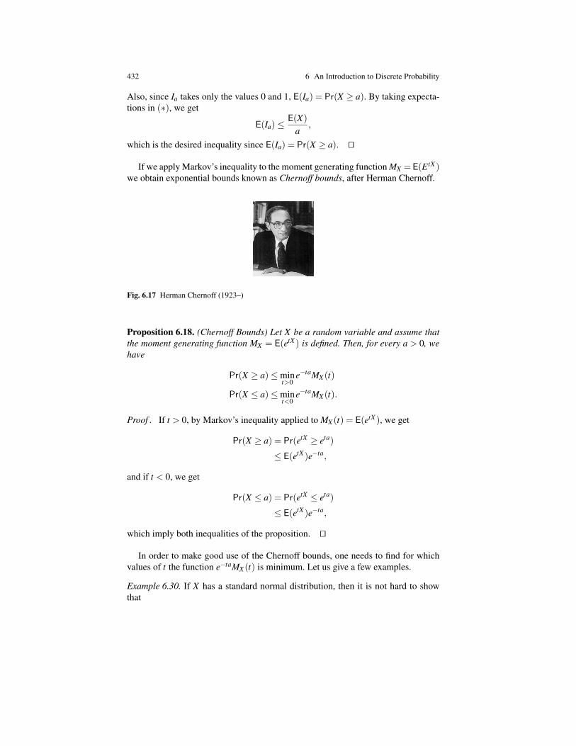
432 6 An Introduction to Discrete Probability
Also, since Ia takes only the values 0 and 1, E(Ia) = Pr(X ≥ a). By taking expecta-tions in (∗), we get
E(Ia)≤E(X)
a,
which is the desired inequality since E(Ia) = Pr(X ≥ a). ut
If we apply Markov’s inequality to the moment generating function MX =E(EtX )we obtain exponential bounds known as Chernoff bounds, after Herman Chernoff.
Fig. 6.17 Herman Chernoff (1923–)
Proposition 6.18. (Chernoff Bounds) Let X be a random variable and assume thatthe moment generating function MX = E(etX ) is defined. Then, for every a > 0, wehave
Pr(X ≥ a)≤mint>0
e−taMX (t)
Pr(X ≤ a)≤mint<0
e−taMX (t).
Proof . If t > 0, by Markov’s inequality applied to MX (t) = E(etX ), we get
Pr(X ≥ a) = Pr(etX ≥ eta)
≤ E(etX )e−ta,
and if t < 0, we get
Pr(X ≤ a) = Pr(etX ≤ eta)
≤ E(etX )e−ta,
which imply both inequalities of the proposition. ut
In order to make good use of the Chernoff bounds, one needs to find for whichvalues of t the function e−taMX (t) is minimum. Let us give a few examples.
Example 6.30. If X has a standard normal distribution, then it is not hard to showthat

6.8 Chernoff Bounds 433
M(t) = et2/2.
Consequently, for any a > 0 and all t > 0, we get
Pr(X ≥ a)≤ e−taet2/2.
The value t that minimizes et2/2−ta is the value that minimizes t2/2− ta, namelyt = a. Thus, for a > 0, we have
Pr(X ≥ a)≤ e−a2/2.
Similarly, for a < 0, we obtain
Pr(X ≤ a)≤ e−a2/2.
The function on the right hand side decays to zero very quickly.
Example 6.31. Let us now consider a random variable X with a Poisson distributionwith parameter λ . It is not hard to show that
M(t) = eλ (et−1).
Applying the Chernoff bound, for any nonnegative integer k and all t > 0, we get
Pr(X ≥ k)≤ eλ (et−1)e−kt .
Using calculus, we can show that the function on the right hand side has a minimumwhen λ (et −1)− kt is minimum, and this is when et = k/λ . If k > λ and if we letet = k/λ in the Chernoff bound, we obtain
Pr(X ≥ k)≤ eλ (k/λ−1)(
λ
k
)k
,
which is equivalent to
Pr(X ≥ k)≤ e−λ (eλ )k
kk .
Our third example is taken from Mitzenmacher and Upfal [10] (Chapter 4).
Example 6.32. Suppose we have a sequence of n random variables X1,X2, . . . ,Xn,such that each Xi is a Bernoulli variable (with value 0 or 1) with probability ofsuccess pi, and assume that these variables are independent. Such sequences areoften called Poisson trials. We wish to apply the Chernoff bounds to the randomvariable
X = X1 + · · ·+Xn.
We have
µ = E(X) =n
∑i=1
E(Xi) =n
∑i=1
pi.

434 6 An Introduction to Discrete Probability
The moment generating function of Xi is given by
MXi(t) = E(etXi)
= piet +(1− pi)
= 1+ pi(et −1).
Using the fact that 1+ x≤ ex for all x ∈ R, we obtain the bound
MXi(t)≤ epi(et−1).
Since the Xi are independent, we know from Section 6.7 that
MX (t) =n
∏i=1
MXi(t)
≤n
∏i=1
epi(et−1)
= e∑ni=1 pi(et−1)
= eµ(et−1).
Therefore,MX (t)≤ eµ(et−1) for all t.
The next step is to apply the Chernoff bounds. Using a little bit of calculus, weobtain the following result proved in Mitzenmacher and Upfal [10] (Chapter 4).
Proposition 6.19. Given n independent Bernoulli variables X1, . . . ,Xn with successprobability pi, if we let µ = ∑
ni=1 pi and X = X1 + · · ·+Xn, then for any δ such that
0 < δ < 1, we have
Pr(|X−µ| ≥ δ µ)≤ 2e−µδ2
3 .
An an application, if the Xi are independent flips of a fair coin (pi = 1/2), thenµ = n/2, and by picking δ = 6lnn
n , it is easy to show that
Pr
(∣∣∣∣X− n2
∣∣∣∣≥ 12
√6n lnn
)≤ 2e−
µδ23 =
2n.
This shows that the concentrations of the number of heads around the mean n/2is very tight. Most of the time, the deviations from the mean are of the orderO(√
n lnn). Another simple calculation using the Chernoff bounds shows that
Pr
(∣∣∣∣X− n2
∣∣∣∣≥ n4
)≤ 2e−
n24 .
This is a much better bound than the bound provided by the Chebyshev inequality:

6.8 Chernoff Bounds 435
Pr
(∣∣∣∣X− n2
∣∣∣∣≥ n4
)≤ 4
n.
Ross [11] and Mitzenmacher and Upfal [10] consider the situation where a gam-bler is equally likely to win or lose one unit on every play. Assuming that theserandom variables Xi are independent, and that
Pr(Xi = 1) = Pr(Xi =−1) =12,
let Sn = ∑ni=1 Xi be the gamblers’s winning after n plays. It is easy that to see that
the moment generating function of Xi is
MXi(t) =et + e−t
2.
Using a little bit of calculus, one finds that
MXi(t)≤ et22 .
Since the Xi are independent, we obtain
MSn(t) =n
∏i=1
MXi(t) = (MXi(t))n ≤ e
nt22 , t > 0.
The Chernoff bound yields
Pr(Sn ≥ a)≤ ent22 −ta, t > 0.
The minimum is achieved for t = a/n, and assuming that a > 0, we get
P(Sn ≥ a)≤ e−a22n , a > 0.
For example, if a = 6, we get
Pr(S10 ≥ 6)≤ e−3620 ≈ 0.1653.
We leave it as exercise to prove that
Pr(Sn ≥ 6) = Pr(gambler wins at least 8 of the first 10 games) =56
1024≈ 0.0547.
Other examples of the use of Chernoff bounds can be found in Mitzenmacherand Upfal [10] and Ross [12]. There are also inequalities giving a lower bound onthe probability Pr(X > 0), where X is a nonnegative random variable; see Ross [12](Chapter 3), which contains other techniques to find bounds on probabilities, andthe Poisson paradigm. Probabilistic methods also play a major role in Motwani andRaghavan [9].
436 6 An Introduction to Discrete Probability
6.9 Summary
This chapter provides an introduction to discrete probability theory. We define prob-ability spaces (finite and countably infinite) and quickly get to random variables. Weemphasize that random variables are more important that their underlying probabil-ity spaces. Notions such as expectation and variance help us to analyze the behaviorof random variables even if their distributions are not known precisely. We give anumber of examples of computations of expectations, including the coupon collec-tor problem and a randomized version of quicksort.
The last three sections of this chapter contain more advanced material and areoptional. The topics of these optional sections are generating functions (includingthe moment generating function and the characteristic function), the limit theorems(weak law of lage numbers, central limit theorem, and strong law of large numbers),and Chernoff bounds.
• We define: a finite discrete probability space (or finite discrete sample space),outcomes (or elementary events), and events.
• a probability measure (or probability distribution) on a sample space.• a discrete probability space.• a σ -algebra.• independent events.• We discuss the birthday problem.• We give examples of random variables.• We present a randomized version of the quicksort algorithm.• We define: random variables, and their probability mass functions and cumula-
tive distribution functions.• absolutely continuous random variables and their probability density functions.• We give examples of: the binomial distribution.• the geometric distribution.• We show how the Poisson distribution arises as the limit of a binomial distribu-
tion when n is large and p is small.• We define a conditional probability.• We present the “Monty Hall Problem.”• We introduce probablity trees (or trees of possibilities).• We prove several of Bayes’ rules.• We define: the product of probability spaces.• independent random variables.• the joint mass function of two random variables, and the marginal mass func-
tions.• the expectation (or expected value, or mean) E(X) = µ of a random variable X .• We prove the linearity of expectation.• We introduce indicator functions (indicator variables).• We define functions of a random variables.• We compute the expected value of the number of comparsions in the random-
ized version of quicksort.
References 437
• We define the variance Var(X) of a random variable X and the standard devia-tion σ of X by σ =
√Var(X).
• We prove that Var(X) = E(X2)− (E(X))2.• We define the moments and the central moments of a random variable.• We prove that if X and Y are uncorrelated random variables, then Var(X +Y ) =
Var(X)+Var(Y ); in particular, this equation holds if X and Y are independent.• We prove: the Cauchy-Schwarz inequality for discrete random variables.• Cheybyshev’s inequality and give some of its applications.
The next three sections are optional.
• We state the weak law of large numbers (Bernoulli’s theorem).• We define the normal distribution (or Gaussian distribution).• We sate the central limit theorem and present an application.• We define various notions of convergence, including almost sure convergence
and convergence in probability.• We state Kolmogorov’s strong law of large numbers.• For a random variable that takes nonnegative integer values, we define the prob-
ability generating function, GX (z) = E(zX ). We show how the derivatives of GXat z = 1 can be used to compute the mean µ and the variance of X .
• If X and Y are independent random variables, then GX+Y = GX GY .• We define the moment generating function MX (t) = E(etX ) and show that
M(n)X (0) = E(Xn).
• If X and Y are independent random variables, then MX+Y = MX MY .• We define: the cumulants of X .• the characteristic function ϕX (t) = E(eitX ) of X and discuss some of its proper-
ties. Unlike the moment generating function, ϕX is defined for all t ∈ R.• If X and Y are independent random variables, then ϕX+Y = ϕX ϕY . The distribu-
tion of a random variable is uniquely determined by its characteristic function.• We prove: Markov’s inequality.• the general Chernoff bounds in terms of the moment generating function.• We compute Chernoff bound for various distributions, including normal and
Poisson.• We obtain Chernoff bounds for Poisson trials (independent Bernoulli trials with
success probablity pi).
Problems
References
1. Joseph Bertrand. Calcul des Probabilites. New York, NY: Chelsea Publishing Company,third edition, 1907.
2. Pierre Bremaud. Markov Chains, Gibbs Fields, Monte Carlo Simulations, and Queues. TAMNo. 31. New York, NY: Springer, third edition, 2001.
438 6 An Introduction to Discrete Probability
3. William Feller. An Introduction to Probability Theory and its Applications, Vol. 1 . NewYork, NY: Wiley, third edition, 1968.
4. William Feller. An Introduction to Probability Theory and its Applications, Vol. 2 . NewYork, NY: Wiley, second edition, 1971.
5. Ronald L. Graham, Donald E. Knuth, and Oren Patashnik. Concrete Mathematics: A Foun-dation For Computer Science. Reading, MA: Addison Wesley, second edition, 1994.
6. Geoffrey Grimmett and David Stirzaker. Probability and Random Processes. Oxford, UK:Oxford University Press, third edition, 2001.
7. Pierre–Simon Laplace. Theorie Analytique des Probabilites, Volume I. Paris, France: EditionsJacques Gabay, third edition, 1820.
8. Pierre–Simon Laplace. Theorie Analytique des Probabilites, Volume II. Paris, France: Edi-tions Jacques Gabay, third edition, 1820.
9. Rajeev Motwani and Prabhakar Raghavan. Randomized Algorithms. Cambridge, UK: Cam-bridge University Press, first edition, 1995.
10. Michael Mitzenmacher and Eli Upfal. Probability and Computing. Randomized Algorithmsand Probabilistic Analysis. Cambridge, UK: Cambridge University Press, first edition, 2005.
11. Sheldon Ross. A First Course in Probability. Upper Saddle River, NJ: Pearson Prentice Hall,eighth edition, 2010.
12. Sheldon Ross. Probability Models for Computer Science. San Diego, CA: Har-court/Academic Press, first edition, 2002.
13. Albert Nikolaevich Shiryaev. Probability. GTM No. 95 . New York, NY: Springer, secondedition, 1995.
14. Santosh S. Venkatesh. The Theory of Probability: Explorations and Applications. Cambridge,UK: Cambridge University Press, first edition, 2012.
Chapter 7Partial Orders, Lattices, Well-FoundedOrderings, Unique Prime Factorization in Z andGCDs, Fibonacci and Lucas Numbers, PublicKey Cryptography and RSA, DistributiveLattices, Boolean Algebras, Heyting Algebras
7.1 Partial Orders
There are two main kinds of relations that play a very important role in mathematicsand computer science:
1. Partial orders2. Equivalence relations
Equivalence relations were studied in Section 3.9. In this section and the nextfew ones, we define partial orders and investigate some of their properties. As weshow, the ability to use induction is intimately related to a very special property ofpartial orders known as well-foundedness.
Intuitively, the notion of order among elements of a set X captures the fact thatsome elements are bigger than others, perhaps more important, or perhaps that theycarry more information. For example, we are all familiar with the natural ordering≤ of the integers
· · · ,−3≤−2≤−1≤ 0≤ 1≤ 2≤ 3≤ ·· · ,
the ordering of the rationals (where
p1
q1≤ p2
q2iff
p2q1− p1q2
q1q2≥ 0,
i.e., p2q1− p1q2 ≥ 0 if q1q2 > 0 else p2q1− p1q2 ≤ 0 if q1q2 < 0), and the orderingof the real numbers. In all of the above orderings, note that for any two numbers aand b, either a≤ b or b≤ a. We say that such orderings are total orderings.
A natural example of an ordering that is not total is provided by the subset or-dering. Given a set X , we can order the subsets of X by the subset relation: A ⊆ B,where A,B are any subsets of X . For example, if X = a,b,c, we have a⊆ a,b.However, note that neither a is a subset of b,c nor b,c is a subset of a. Wesay that a and b,c are incomparable. Now, not all relations are partial orders, sowhich properties characterize partial orders? Our next definition gives us the answer.
439

440 7 Partial Orders, GCDs, RSA, Lattices
Definition 7.1. A binary relation≤ on a set X is a partial order (or partial ordering)iff it is reflexive, transitive, and antisymmetric; that is:
(1) (Reflexivity): a≤ a, for all a ∈ X .(2) (Transitivity): If a≤ b and b≤ c, then a≤ c, for all a,b,c ∈ X .(3) (Antisymmetry): If a≤ b and b≤ a, then a = b, for all a,b ∈ X .
A partial order is a total order (ordering) (or linear order (ordering)) iff for alla,b ∈ X , either a ≤ b or b ≤ a. When neither a ≤ b nor b ≤ a, we say that a and bare incomparable. A subset, C ⊆ X , is a chain iff ≤ induces a total order on C (so,for all a,b ∈C, either a≤ b or b≤ a). A subset, C ⊆ X , is an antichain iff any twodistinct elements in C are incomparable. The strict order (ordering) < associatedwith ≤ is the relation defined by: a < b iff a≤ b and a 6= b. If ≤ is a partial order onX , we say that the pair 〈X ,≤〉 is a partially ordered set or for short, a poset.
Remark: Observe that if < is the strict order associated with a partial order≤, then< is transitive and antireflexive, which means that
(4) a 6< a, for all a ∈ X .
Conversely, let < be a relation on X and assume that < is transitive and antireflexive.Then, we can define the relation≤ so that a≤ b iff a = b or a < b. It is easy to checkthat ≤ is a partial order and that the strict order associated with ≤ is our originalrelation, <.
The concept of antichain is the version for posets of the notion of independent (orstable) set in a graph (usually undirected) introduced in Problem 4.17 and definedofficially in Definition 8.20.
Given a poset 〈X ,≤〉, by abuse of notation we often refer to 〈X ,≤〉 as the posetX , the partial order ≤ being implicit. If confusion may arise, for example, when weare dealing with several posets, we denote the partial order on X by ≤X .
Here are a few examples of partial orders.
1. The subset ordering. We leave it to the reader to check that the subset relation⊆ on a set X is indeed a partial order. For example, if A⊆ B and B⊆ A, whereA,B ⊆ X , then A = B, because these assumptions are exactly those needed bythe extensionality axiom.
2. The natural order on N. Although we all know what the ordering of the naturalnumbers is, we should realize that if we stick to our axiomatic presentationwhere we defined the natural numbers as sets that belong to every inductive set(see Definition 2.11), then we haven’t yet defined this ordering. However, thisis easy to do because the natural numbers are sets. For any m,n ∈ N, definem≤ n as m = n or m ∈ n. Then, it is not hard to check that this relation is a totalorder. (Actually, some of the details are a bit tedious and require induction; seeEnderton [6], Chapter 4.)
3. Orderings on strings. Let Σ = a1, . . . ,an be an alphabet. The prefix, suffix,and substring relations defined in Section 3.15 are easily seen to be partial or-ders. However, these orderings are not total. It is sometimes desirable to have a
7.1 Partial Orders 441
total order on strings and, fortunately, the lexicographic order (also called dic-tionnary order) achieves this goal. In order to define the lexicographic orderwe assume that the symbols in Σ are totally ordered, a1 < a2 < · · ·< an. Then,given any two strings u,v ∈ Σ ∗ we set
u v
if v = uy, for some y ∈ Σ ∗, orif u = xaiy, v = xa jz,and ai < a j, for some x,y,z ∈ Σ ∗.
In other words, either u is a prefix of v or else u and v share a common prefixx, and then there is a differing symbol, ai in u and a j in v, with ai < a j. It isfairly tedious to prove that the lexicographic order is a partial order. Moreover,the lexicographic order is a total order.
4. The divisibility order on N. Let us begin by defining divisibility in Z. Givenany two integers, a,b ∈ Z, with b 6= 0, we say that b divides a (a is a multipleof b) iff a = bq for some q ∈ Z. Such a q is called the quotient of a and b.Most number theory books use the notation b | a to express that b divides a. Forexample, 4 | 12 because 12 = 4 · 3 and 7 | −21 because −21 = 7 · (−3) but 3does not divide 16 because 16 is not an integer multiple of 3.We leave the verification that the divisibility relation is reflexive and transitiveas an easy exercise. What about antisymmetry? So, assume that b | a and a | b(thus, a,b 6= 0). This means that there exist q1,q2 ∈ Z so that
a = bq1 and b = aq2.
From the above, we deduce that b = bq1q2; that is,
b(1−q1q2) = 0.
As b 6= 0, we conclude thatq1q2 = 1.
Now, let us restrict ourselves to N+ = N−0, so that a,b ≥ 1. It follows thatq1,q2 ∈ N and in this case, q1q2 = 1 is only possible iff q1 = q2 = 1. There-fore, a = b and the divisibility relation is indeed a partial order on N+. Why isdivisibility not a partial order on Z−0?
Given a poset 〈X ≤〉, if X is finite then there is a convenient way to describe thepartial order≤ on X using a graph. In preparation for that, we need a few preliminarynotions.
Consider an arbitrary poset 〈X ≤〉 (not necessarily finite). Given any elementa ∈ X , the following situations are of interest.
1. For no b ∈ X do we have b < a. We say that a is a minimal element (of X).2. There is some b ∈ X so that b < a and there is no c ∈ X so that b < c < a. We
say that b is an immediate predecessor of a.3. For no b ∈ X do we have a < b. We say that a is a maximal element (of X).
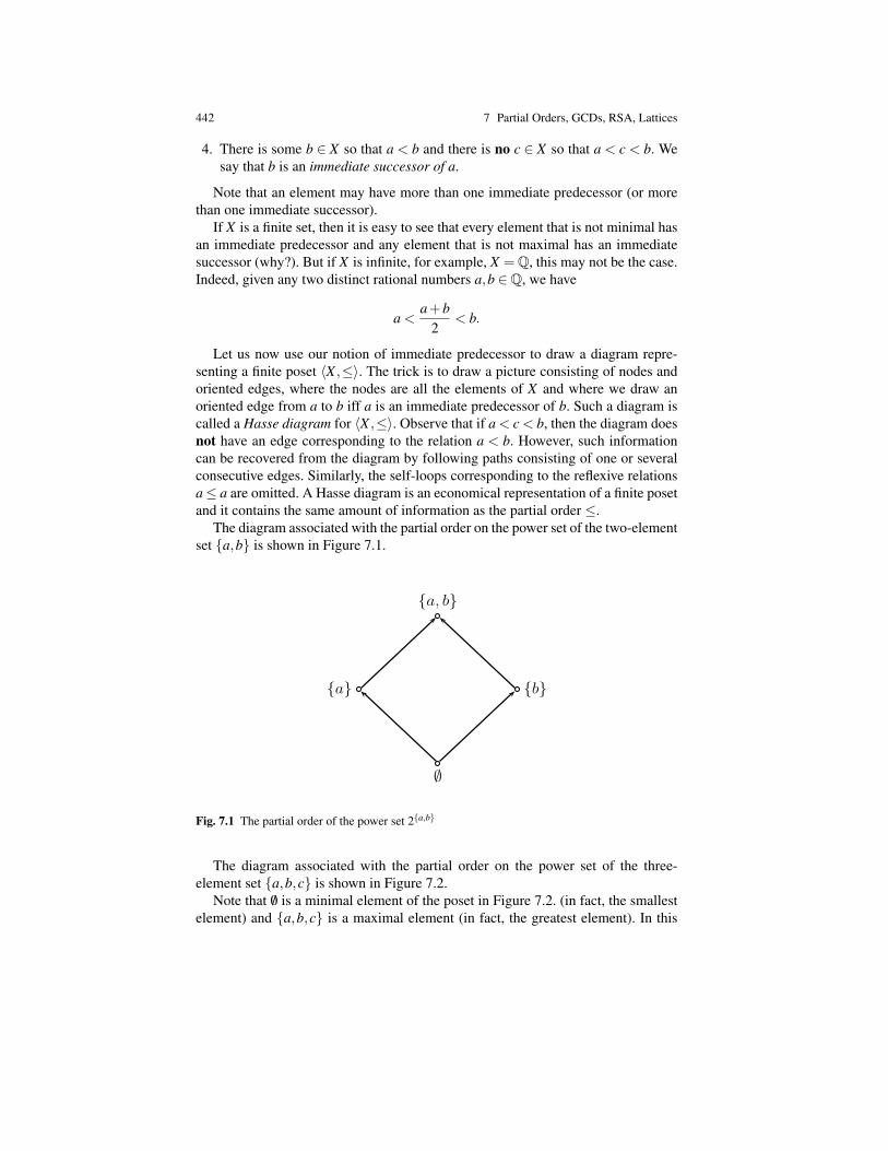
442 7 Partial Orders, GCDs, RSA, Lattices
4. There is some b ∈ X so that a < b and there is no c ∈ X so that a < c < b. Wesay that b is an immediate successor of a.
Note that an element may have more than one immediate predecessor (or morethan one immediate successor).
If X is a finite set, then it is easy to see that every element that is not minimal hasan immediate predecessor and any element that is not maximal has an immediatesuccessor (why?). But if X is infinite, for example, X =Q, this may not be the case.Indeed, given any two distinct rational numbers a,b ∈Q, we have
a <a+b
2< b.
Let us now use our notion of immediate predecessor to draw a diagram repre-senting a finite poset 〈X ,≤〉. The trick is to draw a picture consisting of nodes andoriented edges, where the nodes are all the elements of X and where we draw anoriented edge from a to b iff a is an immediate predecessor of b. Such a diagram iscalled a Hasse diagram for 〈X ,≤〉. Observe that if a < c < b, then the diagram doesnot have an edge corresponding to the relation a < b. However, such informationcan be recovered from the diagram by following paths consisting of one or severalconsecutive edges. Similarly, the self-loops corresponding to the reflexive relationsa≤ a are omitted. A Hasse diagram is an economical representation of a finite posetand it contains the same amount of information as the partial order ≤.
The diagram associated with the partial order on the power set of the two-elementset a,b is shown in Figure 7.1.
1
!
a b
a, b
Fig. 7.1 The partial order of the power set 2a,b
The diagram associated with the partial order on the power set of the three-element set a,b,c is shown in Figure 7.2.
Note that /0 is a minimal element of the poset in Figure 7.2. (in fact, the smallestelement) and a,b,c is a maximal element (in fact, the greatest element). In this

7.1 Partial Orders 443
1
!
a b c
b, c a, c a, b
a, b, c
Fig. 7.2 The partial order of the power set 2a,b,c
example, there is a unique minimal (respectively, maximal) element. A less trivialexample with multiple minimal and maximal elements is obtained by deleting /0 anda,b,c and is shown in Figure 7.3.
1
a b c
b, c a, c a, b
Fig. 7.3 Minimal and maximal elements in a poset
Given a poset 〈X ,≤〉, observe that if there is some element m ∈ X so that m≤ xfor all x ∈ X , then m is unique. Indeed, if m′ is another element so that m′ ≤ x for allx∈ X , then if we set x = m′ in the first case, we get m≤m′ and if we set x = m in thesecond case, we get m′ ≤ m, from which we deduce that m = m′, as claimed. Suchan element m, is called the smallest or the least element of X . Similarly, an elementb ∈ X , so that x ≤ b for all x ∈ X is unique and is called the greatest or the largestelement of X .
We summarize some of our previous definitions and introduce a few more usefulconcepts in the following.

444 7 Partial Orders, GCDs, RSA, Lattices
Definition 7.2. Let 〈X ,≤〉 be a poset and let A⊆ X be any subset of X . An elementb ∈ X is a lower bound of A iff b ≤ a for all a ∈ A. An element m ∈ X is an upperbound of A iff a ≤ m for all a ∈ A. An element b ∈ X is the least element of A iffb ∈ A and b ≤ a for all a ∈ A. An element m ∈ X is the greatest element of A iffm ∈ A and a ≤ m for all a ∈ A. An element b ∈ A is minimal in A iff a < b for noa ∈ A, or equivalently, if for all a ∈ A, a≤ b implies that a = b. An element m ∈ A ismaximal in A iff m < a for no a ∈ A, or equivalently, if for all a ∈ A, m≤ a impliesthat a = m. An element b ∈ X is the greatest lower bound of A iff the set of lowerbounds of A is nonempty and if b is the greatest element of this set. An elementm ∈ X is the least upper bound of A iff the set of upper bounds of A is nonemptyand if m is the least element of this set.
Remarks:
1. If b is a lower bound of A (or m is an upper bound of A), then b (or m) may notbelong to A.
2. The least element of A is a lower bound of A that also belongs to A and thegreatest element of A is an upper bound of A that also belongs to A. The leastelement of a subset A is also called the minimum of A, and greatest elementof a subset A is also called the maximum of A, When A = X , the least elementis often denoted ⊥, sometimes 0, and the greatest element is often denoted >,sometimes 1.
3. Minimal or maximal elements of A belong to A but they are not necessarilyunique.
The greatest lower bound (or the least upper bound) of A may not belong to A.We use the notation
∧A for the greatest lower bound of A and the notation
∨A for
the least upper bound of A. In computer science, some people also use⊔
A insteadof∨
A and the symbol⊔
upside down instead of∧
. When A = a,b, we write a∧bfor
∧a,b and a∨ b for∨a,b. The element a∧ b is called the meet of a and b
and a∨ b is the join of a and b. (Some computer scientists use au b for a∧ b andatb for a∨b.)
Observe that if it exists,∧
/0 = >, the greatest element of X and if its exists,∨/0 =⊥, the least element of X . Also, if it exists,
∧X =⊥ and if it exists,
∨X =>.
The reader should look at the posets in Figures 7.2 and 7.3 for examples of theabove notions.
For the sake of completeness, we state the following fundamental result known asZorn’s lemma even though it is unlikely that we use it in this course. Zorn’s lemmaturns out to be equivalent to the axiom of choice. For details and a proof, the readeris referred to Suppes [16] or Enderton [6].
Theorem 7.1. (Zorn’s Lemma) Given a poset 〈X ,≤〉, if every nonempty chain in Xhas an upper bound, then X has some maximal element.
When we deal with posets, it is useful to use functions that are order preservingas defined next.
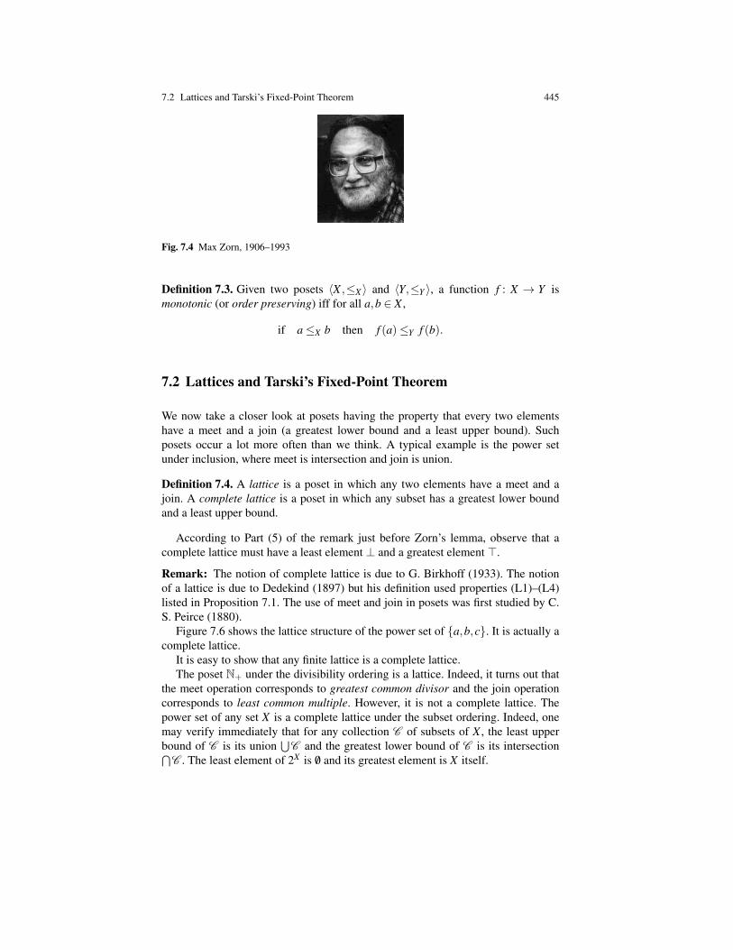
7.2 Lattices and Tarski’s Fixed-Point Theorem 445
Fig. 7.4 Max Zorn, 1906–1993
Definition 7.3. Given two posets 〈X ,≤X 〉 and 〈Y,≤Y 〉, a function f : X → Y ismonotonic (or order preserving) iff for all a,b ∈ X ,
if a≤X b then f (a)≤Y f (b).
7.2 Lattices and Tarski’s Fixed-Point Theorem
We now take a closer look at posets having the property that every two elementshave a meet and a join (a greatest lower bound and a least upper bound). Suchposets occur a lot more often than we think. A typical example is the power setunder inclusion, where meet is intersection and join is union.
Definition 7.4. A lattice is a poset in which any two elements have a meet and ajoin. A complete lattice is a poset in which any subset has a greatest lower boundand a least upper bound.
According to Part (5) of the remark just before Zorn’s lemma, observe that acomplete lattice must have a least element ⊥ and a greatest element >.
Remark: The notion of complete lattice is due to G. Birkhoff (1933). The notionof a lattice is due to Dedekind (1897) but his definition used properties (L1)–(L4)listed in Proposition 7.1. The use of meet and join in posets was first studied by C.S. Peirce (1880).
Figure 7.6 shows the lattice structure of the power set of a,b,c. It is actually acomplete lattice.
It is easy to show that any finite lattice is a complete lattice.The poset N+ under the divisibility ordering is a lattice. Indeed, it turns out that
the meet operation corresponds to greatest common divisor and the join operationcorresponds to least common multiple. However, it is not a complete lattice. Thepower set of any set X is a complete lattice under the subset ordering. Indeed, onemay verify immediately that for any collection C of subsets of X , the least upperbound of C is its union
⋃C and the greatest lower bound of C is its intersection⋂
C . The least element of 2X is /0 and its greatest element is X itself.
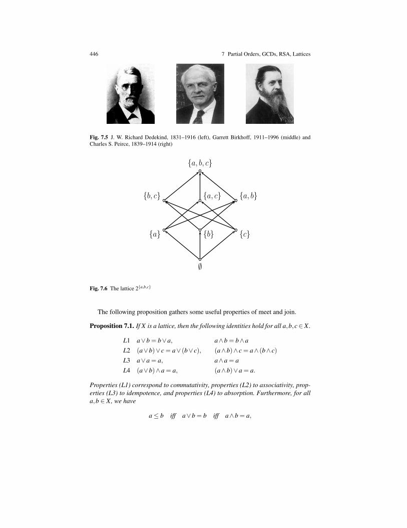
446 7 Partial Orders, GCDs, RSA, Lattices
Fig. 7.5 J. W. Richard Dedekind, 1831–1916 (left), Garrett Birkhoff, 1911–1996 (middle) andCharles S. Peirce, 1839–1914 (right)
1
!
a b c
b, c a, c a, b
a, b, c
Fig. 7.6 The lattice 2a,b,c
The following proposition gathers some useful properties of meet and join.
Proposition 7.1. If X is a lattice, then the following identities hold for all a,b,c∈X.
L1 a∨b = b∨a, a∧b = b∧a
L2 (a∨b)∨ c = a∨ (b∨ c), (a∧b)∧ c = a∧ (b∧ c)
L3 a∨a = a, a∧a = a
L4 (a∨b)∧a = a, (a∧b)∨a = a.
Properties (L1) correspond to commutativity, properties (L2) to associativity, prop-erties (L3) to idempotence, and properties (L4) to absorption. Furthermore, for alla,b ∈ X, we have
a≤ b iff a∨b = b iff a∧b = a,

7.2 Lattices and Tarski’s Fixed-Point Theorem 447
called consistency.
Proof . The proof is left as an exercise to the reader. ut
Properties (L1)–(L4) are algebraic identities that were found by Dedekind (1897).A pretty symmetry reveals itself in these identities: they all come in pairs, one in-volving ∧, the other involving ∨. A useful consequence of this symmetry is duality,namely, that each equation derivable from (L1)–(L4) has a dual statement obtainedby exchanging the symbols ∧ and ∨. What is even more interesting is that it is pos-sible to use these properties to define lattices. Indeed, if X is a set together withtwo operations ∧ and ∨ satisfying (L1)–(L4), we can define the relation a ≤ b bya∨ b = b and then show that ≤ is a partial order such that ∧ and ∨ are the corre-sponding meet and join. The first step is to show that
a∨b = b iff a∧b = a.
If a∨b = b, then substituting b for a∨b in (L4), namely
(a∨b)∧a = a,
we getb∧a = a,
which, by (L1), yieldsa∧b = a,
as desired. Conversely, if a∧b = a, then by (L1) we have b∧a = a, and substitutinga for b∧a in the instance of (L4) where a and b are switched, namely
(b∧a)∨b = b,
we geta∨b = b,
as claimed. Therefore, we can define a≤ b as a∨b = b or equivalently as a∧b = a.After a little work, we obtain the following proposition.
Proposition 7.2. Let X be a set together with two operations ∧ and ∨ satisfying theaxioms (L1)–(L4) of Proposition 7.1. If we define the relation≤ by a≤ b iff a∨b= b(equivalently, a∧b = a), then≤ is a partial order and (X ,≤) is a lattice whose meetand join agree with the original operations ∧ and ∨.
The following proposition shows that the existence of arbitrary least upperbounds (or arbitrary greatest lower bounds) is already enough ensure that a posetis a complete lattice.
Proposition 7.3. Let 〈X ,≤〉 be a poset. If X has a greatest element >, and if everynonempty subset A of X has a greatest lower bound
∧A, then X is a complete lattice.
Dually, if X has a least element ⊥ and if every nonempty subset A of X has a leastupper bound
∨A, then X is a complete lattice
448 7 Partial Orders, GCDs, RSA, Lattices
Proof . Assume X has a greatest element > and that every nonempty subset A ofX has a greatest lower bound,
∧A. We need to show that any subset S of X has a
least upper bound. As X has a greatest element >, the set U of upper bounds of Sis nonempty and so, m =
∧U exists. We claim that
∧U =
∨S (i.e., m is the least
upper bound of S). First, note that every element of S is a lower bound of U becauseU is the set of upper bounds of S. As m =
∧U is the greatest lower bound of U ,
we deduce that s≤ m for all s ∈ S (i.e., m is an upper bound of S). Next, if b is anyupper bound for S, then b ∈U and as m is a lower bound of U (the greatest one), wehave m≤ b (i.e., m is the least upper bound of S). The other statement is proved byduality. ut
We are now going to prove a remarkable result due to A. Tarski (discovered in1942, published in 1955). A special case (for power sets) was proved by B. Knaster(1928). First, we define fixed points.
Fig. 7.7 Alferd Tarski, 1902–1983
Definition 7.5. Let 〈X ,≤〉 be a poset and let f : X → X be a function. An elementx ∈ X is a fixed point of f (sometimes spelled fixpoint) iff
f (x) = x.
An element, x ∈ X , is a least (respectively, greatest) fixed point of f if it is a fixedpoint of f and if x≤ y (resp. y≤ x) for every fixed point y of f .
Fixed points play an important role in certain areas of mathematics (e.g., topol-ogy, differential equations) and also in economics because they tend to capture thenotion of stability or equilibrium.
We now prove the following pretty theorem due to Tarski and then immediatelyproceed to use it to give a very short proof of the Schroder–Bernstein theorem (The-orem 3.9).
Theorem 7.2. (Tarski’s Fixed-Point Theorem) Let 〈X ,≤〉 be a complete lattice andlet f : X → X be any monotonic function. Then, the set F of fixed points of f is acomplete lattice. In particular, f has a least fixed point,
7.2 Lattices and Tarski’s Fixed-Point Theorem 449
xmin =∧x ∈ X | f (x)≤ x
and a greatest fixed point
xmax =∨x ∈ X | x≤ f (x).
Proof . We proceed in three steps.Step 1. We prove that xmax is the largest fixed point of f .Because xmax is an upper bound of A = x ∈ X | x ≤ f (x) (the smallest one),
we have x ≤ xmax for all x ∈ A. By monotonicity of f , we get f (x) ≤ f (xmax) andbecause x ∈ A, we deduce
x≤ f (x)≤ f (xmax) for all x ∈ A,
which shows that f (xmax) is an upper bound of A. As xmax is the least upper boundof A, we get
xmax ≤ f (xmax). (∗)Again, by monotonicity, from the above inequality, we get
f (xmax)≤ f ( f (xmax)),
which shows that f (xmax) ∈ A. As xmax is an upper bound of A, we deduce that
f (xmax)≤ xmax. (∗∗)
But then, (∗) and (∗∗) yieldf (xmax) = xmax,
which shows that xmax is a fixed point of f . If x is any fixed point of f , that is, iff (x) = x, we also have x ≤ f (x); that is, x ∈ A. As xmax is the least upper bound ofA, we have x≤ xmax, which proves that xmax is the greatest fixed point of f .
Step 2. We prove that xmin is the least fixed point of f .This proof is dual to the proof given in Step 1.Step 3. We know that the set of fixed points F of f has a least element and a
greatest element, so by Proposition 7.3, it is enough to prove that any nonemptysubset S⊆ F has a greatest lower bound. If we let
I = x ∈ X | x≤ s for all s ∈ S and x≤ f (x),
then we claim that a =∨
I is a fixed point of f and that it is the greatest lower boundof S.
The proof that a =∨
I is a fixed point of f is analogous to the proof used in Step1. Because a is an upper bound of I, we have x≤ a for all x ∈ I. By monotonicity off and the fact that x ∈ I, we get
x≤ f (x)≤ f (a).
450 7 Partial Orders, GCDs, RSA, Lattices
Thus, f (a) is an upper bound of I and so, as a is the least upper bound of I, we have
a≤ f (a). (†)
By monotonicity of f , we get f (a)≤ f ( f (a)). Now, to claim that f (a) ∈ I, we needto check that f (a) is a lower bound of S. However, by definition of I, every elementof S is an upper bound of I and because a is the least upper bound of I, we musthave a ≤ s for all s ∈ S; that is, a is a lower bound of S. By monotonicity of f andthe fact that S is a set of fixed points, we get
f (a)≤ f (s) = s, for all s ∈ S,
which shows that f (a) is a lower bound of S and thus, f (a) ∈ I, as contended. As ais an upper bound of I and f (a) ∈ I, we must have
f (a)≤ a, (††)
and together with (†), we conclude that f (a) = a; that is, a is a fixed point of f .We already proved that a is a lower bound of S thus it only remains to show that
if x is any fixed point of f and x is a lower bound of S, then x ≤ a. But, if x is anyfixed point of f then x ≤ f (x) and because x is also a lower bound of S, then x ∈ I.As a is an upper bound of I, we do get x≤ a. ut
It should be noted that the least upper bounds and the greatest lower bounds inF do not necessarily agree with those in X . In technical terms, F is generally not asublattice of X .
Now, as promised, we use Tarski’s fixed-point theorem to prove the Schroder–Bernstein theorem.
Theorem 3.9 Given any two sets A and B, if there is an injection from A to Band an injection from B to A, then there is a bijection between A and B.Proof . Let f : A→ B and g : B→ A be two injections. We define the functionϕ : 2A→ 2A by
ϕ(S) = A−g(B− f (S)),
for any S ⊆ A. Because of the two complementations, it is easy to check that ϕ ismonotonic (check it). As 2A is a complete lattice, by Tarski’s fixed point theorem,the function ϕ has a fixed point; that is, there is some subset C ⊆ A so that
C = A−g(B− f (C)).
By taking the complement of C in A, we get
A−C = g(B− f (C)).
Now, as f and g are injections, the restricted functions f C : C→ f (C) andg (B− f (C)) : (B− f (C))→ (A−C) are bijections. Using these functions, wedefine the function h : A→ B as follows.
7.3 Well-Founded Orderings and Complete Induction 451
h(a) =
f (a) if a ∈C(g (B− f (C))−1(a) if a /∈C.
The reader may check that h is indeed a bijection. ut
The above proof is probably the shortest known proof of the Schroder–Bernsteintheorem because it uses Tarski’s fixed-point theorem, a powerful result. If one lookscarefully at the proof, one realizes that there are two crucial ingredients:
1. The set C is closed under g f ; that is, g f (C)⊆C.2. A−C ⊆ g(B).
Using these observations, it is possible to give a proof that circumvents the useof Tarski’s theorem. Such a proof is given in Enderton [6], Chapter 6, and we give asketch of this proof below.
Define a sequence of subsets Cn of A by recursion as follows.
C0 = A−g(B)
Cn+1 = (g f )(Cn),
and setC =
⋃n≥0
Cn.
Clearly, A−C ⊆ g(B) and because direct images preserve unions, (g f )(C) ⊆C.The definition of h is similar to the one used in our proof:
h(a) =
f (a) if a ∈C(g (A−C))−1(a) if a /∈C.
When a /∈C, that is, a ∈ A−C, as A−C ⊆ g(B) and g is injective, g−1(a) is indeedwell-defined. As f and g are injective, so is g−1 on A−C. So, to check that h is in-jective, it is enough to prove that f (a) = g−1(b) with a ∈C and b /∈C is impossible.However, if f (a) = g−1(b), then (g f )(a) = b. Because (g f )(C)⊆C and a ∈C,we get b = (g f )(a) ∈C, yet b /∈C, a contradiction. It is not hard to verify that h issurjective and therefore, h is a bijection between A and B. ut
The classical reference on lattices is Birkhoff [1]. We highly recommend thisbeautiful book (but it is not easy reading).
We now turn to special properties of partial orders having to do with induction.
7.3 Well-Founded Orderings and Complete Induction
Have you ever wondered why induction on N actually “works”? The answer, ofcourse, is that N was defined in such a way that, by Theorem 2.4, it is the “smallest”inductive set. But this is not a very illuminating answer. The key point is that everynonempty subset of N has a least element. This fact is intuitively clear inasmuch

452 7 Partial Orders, GCDs, RSA, Lattices
as if we had some nonempty subset of N with no smallest element, then we couldconstruct an infinite strictly decreasing sequence, k0 > k1 > · · ·> kn > · · · . But thisis absurd, as such a sequence would eventually run into 0 and stop. It turns out thatthe deep reason why induction “works” on a poset is indeed that the poset orderinghas a very special property and this leads us to the following definition.
Definition 7.6. Given a poset 〈X ,≤〉 we say that ≤ is a well-order (well-ordering)and that X is well-ordered by ≤ iff every nonempty subset of X has a least element.
When X is nonempty, if we pick any two-element subset a,b of X , because thesubset a,b must have a least element, we see that either a ≤ b or b ≤ a; that is,every well-order is a total order. First, let us confirm that N is indeed well-ordered.
Theorem 7.3. (Well-Ordering of N) The set of natural numbers N is well-ordered.
Proof . Not surprisingly we use induction, but we have to be a little shrewd. Let Abe any nonempty subset of N. We prove by contradiction that A has a least element.So, suppose A does not have a least element and let P(m) be the predicate
P(m)≡ (∀k ∈ N)(k < m⇒ k /∈ A),
which says that no natural number strictly smaller than m is in A. We prove byinduction on m that P(m) holds. But then, the fact that P(m) holds for all m showsthat A = /0, a contradiction.
Let us now prove P(m) by induction. The base case P(0) holds trivially. Next,assume P(m) holds; we want to prove that P(m+ 1) holds. Pick any k < m+ 1.Then, either
(1) k < m, in which case, by the induction hypothesis, k /∈ A; or(2) k = m. By the induction hypothesis, P(m) holds. Now, if m were in A, as P(m)
holds no k < m would belong to A and m would be the least element of A,contradicting the assumption that A has no least element. Therefore, m /∈ A.
Thus in both cases we proved that if k <m+1, then k /∈A, establishing the inductionhypothesis. This concludes the induction and the proof of Theorem 7.3. ut
Theorem 7.3 yields another induction principle which is often more flexible thanour original induction principle. This principle, called complete induction (or some-times strong induction), was already encountered in Section 3.3. It turns out that itis a special case of induction on a well-ordered set but it does not hurt to review itin the special case of the natural ordering on N. Recall that N+ = N−0.Complete Induction Principle on N.In order to prove that a predicate P(n) holds for all n ∈ N it is enough to prove that
(1) P(0) holds (the base case).(2) For every m ∈ N+, if (∀k ∈ N)(k < m⇒ P(k)) then P(m).

7.3 Well-Founded Orderings and Complete Induction 453
As a formula, complete induction is stated as
P(0)∧ (∀m ∈ N+)[(∀k ∈ N)(k < m⇒ P(k))⇒ P(m)]⇒ (∀n ∈ N)P(n).
The difference between ordinary induction and complete induction is that in com-plete induction, the induction hypothesis (∀k∈N)(k <m⇒P(k)) assumes that P(k)holds for all k < m and not just for m−1 (as in ordinary induction), in order to de-duce P(m). This gives us more proving power as we have more knowledge in orderto prove P(m).
We have many occasions to use complete induction but let us first check that itis a valid principle. Even though we already sketched how the validity of completeinduction is a consequence of the (ordinary) induction principle (Version 3) on Nin Section 3.3 and we soon give a more general proof of the validity of completeinduction for a well-ordering, we feel that it is helpful to give the proof in the caseof N as a warm-up.
Theorem 7.4. The complete induction principle for N is valid.
Proof . Let P(n) be a predicate on N and assume that P(n) satisfies Conditions (1)and (2) of complete induction as stated above. We proceed by contradiction. So,assume that P(n) fails for some n ∈ N. If so, the set
F = n ∈ N | P(n) = false
is nonempty. By Theorem 7.3, the set A has a least element m and thus
P(m) = false.
Now, we can’t have m = 0, as we assumed that P(0) holds (by (1)) and because mis the least element for which P(m) = false, we must have
P(k) = true for all k < m.
But, this is exactly the premise in (2) and as we assumed that (2) holds, we deducethat
P(m) = true,
contradicting the fact that we already know that P(m) = false. Therefore, P(n) musthold for all n ∈ N. ut
Remark: In our statement of the principle of complete induction, we singled outthe base case (1), and consequently we stated the induction step (2) for every m ∈N+, excluding the case m = 0, which is already covered by the base case. It is alsopossible to state the principle of complete induction in a more concise fashion asfollows.
(∀m ∈ N)[(∀k ∈ N)(k < m⇒ P(k))⇒ P(m)]⇒ (∀n ∈ N)P(n).
454 7 Partial Orders, GCDs, RSA, Lattices
In the above formula, observe that when m = 0, which is now allowed, the premise(∀k ∈ N)(k < m⇒ P(k)) of the implication within the brackets is trivially true andso, P(0) must still be established. In the end, exactly the same amount of work isrequired but some people prefer the second more concise version of the principleof complete induction. We feel that it would be easier for the reader to make thetransition from ordinary induction to complete induction if we make explicit thefact that the base case must be established.
Let us illustrate the use of the complete induction principle by proving that everynatural number factors as a product of primes. Recall that for any two natural num-bers, a,b ∈ N with b 6= 0, we say that b divides a iff a = bq, for some q ∈ N. In thiscase, we say that a is divisible by b and that b is a factor of a. Then, we say that anatural number p∈N is a prime number (for short, a prime) if p≥ 2 and if p is onlydivisible by itself and by 1. Any prime number but 2 must be odd but the converseis false. For example, 2,3,5,7,11,13,17 are prime numbers, but 9 is not. There areinfinitely many prime numbers but to prove this, we need the following theorem.
Theorem 7.5. Every natural number n≥ 2 can be factored as a product of primes;that is, n can be written as a product n = pm1
1 · · · pmkk , where the pis are pairwise
distinct prime numbers and mi ≥ 1 (1≤ i≤ k).
Proof . We proceed by complete induction on n≥ 2. The base case, n = 2 is trivial,inasmuch as 2 is prime.
Consider any n > 2 and assume that the induction hypothesis holds; that is, everym with 2≤ m < n can be factored as a product of primes. There are two cases.
(a) The number n is prime. Then, we are done.(b) The number n is not a prime. In this case, n factors as n = n1n2, where
2 ≤ n1,n2 < n. By the induction hypothesis, n1 has some prime factorizationand so does n2. If p1, . . . , pk is the union of all the primes occurring in thesefactorizations of n1 and n2, we can write
n1 = pi11 · · · p
ikk and n2 = p j1
1 · · · pjkk ,
where ih, jh ≥ 0 and, in fact, ih + jh ≥ 1, for 1≤ h≤ k. Consequently, n factorsas the product of primes,
n = pi1+ j11 · · · pik+ jk
k ,
with ih + jh ≥ 1, establishing the induction hypothesis. ut
For example, 21 = 31 ·71, 98 = 21 ·72, and 396 = 22 ·33 ·11.
Remark: The prime factorization of a natural number is unique up to permutationof the primes p1, . . . , pk but this requires the Euclidean division lemma. However,we can prove right away that there are infinitely primes.
Theorem 7.6. Given any natural number n≥ 1 there is a prime number p such thatp > n. Consequently, there are infinitely many primes.

7.3 Well-Founded Orderings and Complete Induction 455
Proof . Let m = n!+1. If m is prime, we are done. Otherwise, by Theorem 7.5, thenumber m has a prime decomposition. We claim that p > n for every prime p in thisdecomposition. If not, 2 ≤ p ≤ n and then p would divide both n!+ 1 and n!, so pwould divide 1, a contradiction. ut
As an application of Theorem 7.3, we prove the Euclidean division lemma forthe integers.
Theorem 7.7. (Euclidean Division Lemma for Z) Given any two integers a,b ∈ Z,with b 6= 0, there is some unique integer q ∈ Z (the quotient) and some uniquenatural number r ∈ N (the remainder or residue), so that
a = bq+ r with 0≤ r < |b|.
Proof . First, let us prove the existence of q and r with the required condition on r.We claim that if we show existence in the special case where a,b ∈ N (with b 6= 0),then we can prove existence in the general case. There are four cases:
1. If a,b ∈ N, with b 6= 0, then we are done.2. If a≥ 0 and b < 0, then −b > 0, so we know that there exist q,r with
a = (−b)q+ r with 0≤ r ≤−b−1.
Then,a = b(−q)+ r with 0≤ r ≤ |b|−1.
3. If a < 0 and b > 0, then −a > 0, so we know that there exist q,r with
−a = bq+ r with 0≤ r ≤ b−1.
Then,a = b(−q)− r with 0≤ r ≤ b−1.
If r = 0, we are done. Otherwise, 1≤ r≤ b−1, which implies 1≤ b−r≤ b−1,so we get
a = b(−q)−b+b− r = b(−(q+1))+b− r with 0≤ b− r ≤ b−1.
4. If a < 0 and b < 0, then −a > 0 and −b > 0, so we know that there exist q,rwith
−a = (−b)q+ r with 0≤ r ≤−b−1.
Then,a = bq− r with 0≤ r ≤−b−1.
If r = 0, we are done. Otherwise, 1≤ r ≤−b−1, which implies 1≤−b− r ≤−b−1, so we get
a = bq+b−b− r = b(q+1)+(−b− r) with 0≤−b− r ≤ |b|−1.
456 7 Partial Orders, GCDs, RSA, Lattices
We are now reduced to proving the existence of q and r when a,b ∈ N with b 6= 0.Consider the set
R = a−bq ∈ N | q ∈ N.Note that a ∈ R by setting q = 0, because a ∈ N. Therefore, R is nonempty. ByTheorem 7.3, the nonempty set R has a least element r. We claim that r ≤ b−1 (ofcourse, r ≥ 0 as R⊆N). If not, then r ≥ b, and so r−b≥ 0. As r ∈ R, there is someq ∈ N with r = a−bq. But now, we have
r−b = a−bq−b = a−b(q+1)
and as r−b≥ 0, we see that r−b ∈ R with r−b < r (because b 6= 0), contradictingthe minimality of r. Therefore, 0≤ r ≤ b−1, proving the existence of q and r withthe required condition on r.
We now go back to the general case where a,b ∈ Z with b 6= 0 and we proveuniqueness of q and r (with the required condition on r). So, assume that
a = bq1 + r1 = bq2 + r2 with 0≤ r1 ≤ |b|−1 and 0≤ r2 ≤ |b|−1.
Now, as 0 ≤ r1 ≤ |b| − 1 and 0 ≤ r2 ≤ |b| − 1, we have |r1− r2| < |b|, and frombq1 + r1 = bq2 + r2, we get
b(q2−q1) = r1− r2,
which yields|b||q2−q1|= |r1− r2|.
Because |r1− r2|< |b|, we must have r1 = r2. Then, from b(q2−q1) = r1− r2 = 0,as b 6= 0, we get q1 = q2, which concludes the proof. ut
For example, 12 = 5 · 2+ 2, 200 = 5 · 40+ 0, and 42823 = 6409× 6+ 4369.The remainder r in the Euclidean division, a = bq+ r, of a by b, is usually denoteda mod b.
We now show that complete induction holds for a very broad class of partialorders called well-founded orderings that subsume well-orderings.
Definition 7.7. Given a poset 〈X ,≤〉, we say that ≤ is a well-founded ordering (or-der) and that X is well founded iff X has no infinite strictly decreasing sequencex0 > x1 > x2 > · · ·> xn > xn+1 > · · · .
The following property of well-founded sets is fundamental.
Proposition 7.4. A poset 〈X ,≤〉 is well founded iff every nonempty subset of X hasa minimal element.
Proof . First, assume that every nonempty subset of X has a minimal element. Ifwe had an infinite strictly decreasing sequence, x0 > x1 > x2 > · · ·> xn > · · · , thenthe set A = xn would have no minimal element, a contradiction. Therefore, X iswell founded.
7.3 Well-Founded Orderings and Complete Induction 457
Now, assume that X is well founded. We prove that A has a minimal elementby contradiction. So, let A be some nonempty subset of X and suppose A has nominimal element. This means that for every a ∈ A, there is some b ∈ A with a > b.Using the axiom of choice (graph version), there is some function g : A→ A withthe property that
a > g(a), for all a ∈ A.
Inasmuch as A is nonempty, we can pick some element, say a ∈ A. By the recursionTheorem (Theorem 3.1), there is a unique function f : N→ A so that
f (0) = a,
f (n+1) = g( f (n)) for all n ∈ N.
But then, f defines an infinite sequence xn with xn = f (n), so that xn > xn+1 forall n ∈ N, contradicting the fact that X is well founded. ut
So, the seemingly weaker condition that there is no infinite strictly decreasingsequence in X is equivalent to the fact that every nonempty subset of X has a minimalelement. If X is a total order, any minimal element is actually a least element and sowe get the following.
Corollary 7.1. A poset, 〈X ,≤〉, is well-ordered iff ≤ is total and X is well founded.
Note that the notion of a well-founded set is more general than that of a well-ordered set, because a well-founded set is not necessarily totally ordered.
Remark: Suppose we can prove some property P by ordinary induction on N.Then, I claim that P can also be proved by complete induction on N. To see this,observe first that the base step is identical. Also, for all m ∈ N+, the implication
(∀k ∈ N)(k < m⇒ P(k))⇒ P(m−1)
holds and because the induction step (in ordinary induction) consists in proving forall m ∈ N+ that
P(m−1)⇒ P(m)
holds, from this implication and the previous implication we deduce that for allm ∈ N+, the implication
(∀k ∈ N)(k < m⇒ P(k))⇒ P(m)
holds, which is exactly the induction step of the complete induction method. So, wesee that complete induction on N subsumes ordinary induction on N. The converseis also true but we leave it as a fun exercise. But now, by Theorem 7.3 (ordinary)induction on N implies that N is well-ordered and by Theorem 7.4, the fact thatN is well-ordered implies complete induction on N. We just showed that completeinduction on N implies (ordinary) induction on N, therefore we conclude that allthree are equivalent; that is,
458 7 Partial Orders, GCDs, RSA, Lattices
(ordinary) induction on N is validiff
complete induction on N is validiff
N is well-ordered.
These equivalences justify our earlier claim that the ability to do induction hingeson some key property of the ordering, in this case, that it is a well-ordering.
We finally come to the principle of complete induction (also called transfiniteinduction or structural induction), which, as we prove, is valid for all well-foundedsets. Every well-ordered set is also well-founded, thus complete induction is a verygeneral induction method.
Let (X ,≤) be a well-founded poset and let P be a predicate on X (i.e., a functionP : X →true, false).Principle of Complete Induction on a Well-Founded Set.To prove that a property P holds for all z ∈ X , it suffices to show that, for everyx ∈ X ,
(∗) If x is minimal or P(y) holds for all y < x,(∗∗) Then P(x) holds.
The statement (∗) is called the induction hypothesis, and the implicationfor all x, (∗) implies (∗∗) is called the induction step. Formally, the induction
principle can be stated as:
(∀x ∈ X)[(∀y ∈ X)(y < x⇒ P(y))⇒ P(x)]⇒ (∀z ∈ X)P(z) (CI)
Note that if x is minimal, then there is no y ∈ X such that y < x, and(∀y ∈ X)(y < x⇒ P(y)) is true. Hence, we must show that P(x) holds for everyminimal element x. These cases are called the base cases.
Complete induction is not valid for arbitrary posets (see the problems) but holdsfor well-founded sets as shown in the following theorem.
Theorem 7.8. The principle of complete induction holds for every well-founded set.
Proof . We proceed by contradiction. Assume that (CI) is false. Then,
(∀x ∈ X)[(∀y ∈ X)(y < x⇒ P(y))⇒ P(x)] (1)
holds and(∀z ∈ X)P(z) (2)
is false, that is, there is some z ∈ X so that
P(z) = false.
Hence, the subset F of X defined by
F = x ∈ X | P(x) = false
7.3 Well-Founded Orderings and Complete Induction 459
is nonempty. Because X is well founded, by Proposition 7.4, F has some minimalelement b. Because (1) holds for all x ∈ X , letting x = b, we see that
[(∀y ∈ X)(y < b⇒ P(y))⇒ P(b)] (3)
holds. If b is also minimal in X , then there is no y ∈ X such that y < b and so,
(∀y ∈ X)(y < b⇒ P(y))
holds trivially and (3) implies that P(b)= true, which contradicts the fact that b∈F .Otherwise, for every y ∈ X such that y < b, P(y) = true, because otherwise y wouldbelong to F and b would not be minimal. But then,
(∀y ∈ X)(y < b⇒ P(y))
also holds and (3) implies that P(b) = true, contradicting the fact that b∈ F . Hence,complete induction is valid for well-founded sets. ut
As an illustration of well-founded sets, we define the lexicographic ordering onpairs. Given a partially ordered set 〈X ,≤〉, the lexicographic ordering << on X×Xinduced by ≤ is defined as follows. For all x,y,x′,y′ ∈ X ,
(x,y)<< (x′,y′) iff either
x = x′ and y = y′ orx < x′ orx = x′ and y < y′.
We leave it as an exercise to check that << is indeed a partial order on X ×X .The following proposition is useful.
Proposition 7.5. If 〈X ,≤〉 is a well-founded set, then the lexicographic ordering<< on X×X is also well-founded.
Proof . We proceed by contradiction. Assume that there is an infinite decreasingsequence (〈xi,yi〉)i in X×X . Then, either,
(1) There is an infinite number of distinct xi, or(2) There is only a finite number of distinct xi.
In case (1), the subsequence consisting of these distinct elements forms a de-creasing sequence in X , contradicting the fact that ≤ is well-founded. In case (2),there is some k such that xi = xi+1, for all i≥ k. By definition of <<, the sequence(yi)i≥k is a decreasing sequence in X , contradicting the fact that ≤ is well-founded.Hence, << is well-founded on X×X . ut
As an illustration of the principle of complete induction, consider the followingexample in which it is shown that a function defined recursively is a total function.
460 7 Partial Orders, GCDs, RSA, Lattices
Example (Ackermann’s Function) The following function, A : N× N → N,known as Ackermann’s function is well known in recursive function theory for itsextraordinary rate of growth. It is defined recursively as follows.
A(x,y) = if x = 0 then y+1else if y = 0 then A(x−1,1)else A(x−1,A(x,y−1)).
We wish to prove that A is a total function. We proceed by complete inductionover the lexicographic ordering on N×N.
1. The base case is x = 0, y = 0. In this case, because A(0,y) = y+1, A(0,0) isdefined and equal to 1.
2. The induction hypothesis is that for any (m,n), A(m′,n′) is defined for all(m′,n′)<< (m,n), with (m,n) 6= (m′,n′).
3. For the induction step, we have three cases:
a. If m = 0, because A(0,y) = y+1, A(0,n) is defined and equal to n+1.b. If m 6= 0 and n = 0, because (m−1,1)<< (m,0) and (m−1,1) 6= (m,0),
by the induction hypothesis, A(m−1,1) is defined, and so A(m,0) is de-fined because it is equal to A(m−1,1).
c. If m 6= 0 and n 6= 0, because (m,n−1)<< (m,n) and (m,n−1) 6= (m,n),by the induction hypothesis, A(m,n−1) is defined. Because (m−1,y)<<(m,z) and (m−1,y) 6= (m,z) no matter what y and z are,(m−1,A(m,n−1)) << (m,n) and (m−1,A(m,n−1)) 6= (m,n), and bythe induction hypothesis, A(m−1,A(m,n−1)) is defined. But this is pre-cisely A(m,n), and so A(m,n) is defined. This concludes the inductionstep.
Hence, A(x,y) is defined for all x,y≥ 0. ut
7.4 Unique Prime Factorization in Z and GCDs
In the previous section, we proved that every natural number n≥ 2 can be factored asa product of primes numbers. In this section, we use the Euclidean division lemmato prove that such a factorization is unique. For this, we need to introduce greatestcommon divisors (gcds) and prove some of their properties.
In this section, it is convenient to allow 0 to be a divisor. So, given any twointegers, a,b ∈ Z, we say that b divides a and that a is a multiple of b iff a = bq,for some q ∈ Z. Contrary to our previous definition, b = 0 is allowed as a divisor.However, this changes very little because if 0 divides a, then a = 0q = 0; that is, theonly integer divisible by 0 is 0. The notation b | a is usually used to denote that bdivides a. For example, 3 | 21 because 21 = 2 · 7, 5 | −20 because −20 = 5 · (−4)but 3 does not divide 20.

7.4 Unique Prime Factorization in Z and GCDs 461
We begin by introducing a very important notion in algebra, that of an ideal dueto Richard Dedekind, and prove a fundamental property of the ideals of Z.
Fig. 7.8 Richard Dedekind, 1831–1916
Definition 7.8. An ideal of Z is any nonempty subset I of Z satisfying the followingtwo properties.
(ID1) If a,b ∈ I, then b−a ∈ I.(ID2) If a ∈ I, then ak ∈ I for every k ∈ Z.
An ideal I is a principal ideal if there is some a ∈ I, called a generator, such thatI = ak | k ∈ Z. The equality I = ak | k ∈ Z is also written as I = aZ or asI= (a). The ideal I= (0) = 0 is called the null ideal.
Note that if I is an ideal, then I=Z iff 1∈ I. Because by definition, an ideal I isnonempty, there is some a ∈ I, and by (ID1) we get 0 = a−a ∈ I. Then, for everya ∈ I, since 0 ∈ I, by (ID1) we get −a ∈ I.
Theorem 7.9. Every ideal I of Z is a principal ideal; that is, I = mZ for someunique m ∈ N, with m > 0 iff I 6= (0).
Proof . Note that I= (0) iff I= 0Z and the theorem holds in this case. So, assumethat I 6= (0). Then, our previous observation that −a ∈ I for every a ∈ I impliesthat some positive integer belongs to I and so, the set I∩N+ is nonempty. As N iswell ordered, this set has a smallest element, say m > 0. We claim that I= mZ.
As m ∈ I, by (ID2), mZ ⊆ I. Conversely, pick any n ∈ I. By the Euclideandivision lemma, there are unique q∈Z and r ∈N so that n=mq+r, with 0≤ r <m.If r > 0, because m ∈ I, by (ID2), mq ∈ I, and by (ID1), we get r = n−mq ∈ I.Yet r < m, contradicting the minimality of m. Therefore, r = 0, so n = mq ∈ mZ,establishing that I ⊆ mZ and thus, I = mZ, as claimed. As to uniqueness, clearly(0) 6= mZ if m 6= 0, so assume mZ= m′Z, with m > 0 and m′ > 0. Then, m dividesm′ and m′ divides m, but we already proved earlier that this implies m = m′. ut
Theorem 7.9 is often phrased: Z is a principal ideal domain, for short, a PID.Note that the natural number m such that I= mZ is a divisor of every element in I.
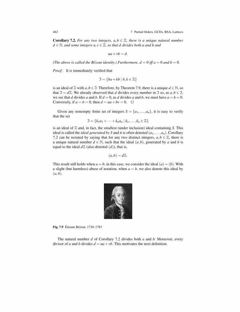
462 7 Partial Orders, GCDs, RSA, Lattices
Corollary 7.2. For any two integers, a,b ∈ Z, there is a unique natural numberd ∈ N, and some integers u,v ∈ Z, so that d divides both a and b and
ua+ vb = d.
(The above is called the Bezout identity.) Furthermore, d = 0 iff a = 0 and b = 0.
Proof . It is immediately verified that
I= ha+ kb | h,k ∈ Z
is an ideal of Z with a,b∈ I. Therefore, by Theorem 7.9, there is a unique d ∈N, sothat I = dZ. We already observed that d divides every number in I so, as a,b ∈ I,we see that d divides a and b. If d = 0, as d divides a and b, we must have a = b = 0.Conversely, if a = b = 0, then d = ua+bv = 0. ut
Given any nonempty finite set of integers S = a1, . . . ,an, it is easy to verifythat the set
I= k1a1 + · · ·+ knan | k1, . . . ,kn ∈ Zis an ideal of Z and, in fact, the smallest (under inclusion) ideal containing S. Thisideal is called the ideal generated by S and it is often denoted (a1, . . . ,an). Corollary7.2 can be restated by saying that for any two distinct integers, a,b ∈ Z, there isa unique natural number d ∈ N, such that the ideal (a,b), generated by a and b isequal to the ideal dZ (also denoted (d)), that is,
(a,b) = dZ.
This result still holds when a = b; in this case, we consider the ideal (a) = (b). Witha slight (but harmless) abuse of notation, when a = b, we also denote this ideal by(a,b).
Fig. 7.9 Etienne Bezout, 1730–1783
The natural number d of Corollary 7.2 divides both a and b. Moreover, everydivisor of a and b divides d = ua+ vb. This motivates the next definition.

7.4 Unique Prime Factorization in Z and GCDs 463
Definition 7.9. Given any two integers a,b ∈ Z, an integer d ∈ Z is a greatest com-mon divisor of a and b (for short, a gcd of a and b) if d divides a and b and, forany integer, h ∈ Z, if h divides a and b, then h divides d. We say that a and b arerelatively prime if 1 is a gcd of a and b.
Remarks:
1. If a = b = 0 then any integer d ∈ Z is a divisor of 0. In particular, 0 divides0. According to Definition 7.9, this implies gcd(0,0) = 0. The ideal generatedby 0 is the trivial ideal (0), so gcd(0,0) = 0 is equal to the generator of thezero ideal, (0).If a 6= 0 or b 6= 0, then the ideal (a,b), generated by a and b is not the zeroideal and there is a unique integer, d > 0, such that
(a,b) = dZ.
For any gcd d′, of a and b, because d divides a and b we see that d must divided′. As d′ also divides a and b, the number d′ must also divide d. Thus, d = d′q′
and d′ = dq for some q,q′ ∈ Z and so, d = dqq′ which implies qq′ = 1 (inas-much as d 6= 0). Therefore, d′ = ±d. So, according to the above definition,when (a,b) 6= (0), gcds are not unique. However, exactly one of d′ or −d′
is positive and equal to the positive generator d, of the ideal (a,b). We referto this positive gcd as “the” gcd of a and b and write d = gcd(a,b). Observethat gcd(a,b) = gcd(b,a). For example, gcd(20,8) = 4, gcd(1000,50) = 50,gcd(42823,6409) = 17, and gcd(5,16) = 1.
2. Another notation commonly found for gcd(a,b) is (a,b), but this is confusingbecause (a,b) also denotes the ideal generated by a and b.
3. Observe that if d = gcd(a,b) 6= 0, then d is indeed the largest positive commondivisor of a and b because every divisor of a and b must divide d. However,we did not use this property as one of the conditions for being a gcd becausesuch a condition does not generalize to other rings where a total order is notavailable. Another minor reason is that if we had used in the definition of agcd the condition that gcd(a,b) should be the largest common divisor of a andb, as every integer divides 0, gcd(0,0) would be undefined.
4. If a = 0 and b > 0, then the ideal (0,b), generated by 0 and b, is equal to theideal (b) = bZ, which implies gcd(0,b) = b and similarly, if a > 0 and b = 0,then gcd(a,0) = a.
Let p ∈ N be a prime number. Then, note that for any other integer n, if p doesnot divide n, then gcd(p,n) = 1, as the only divisors of p are 1 and p.
Proposition 7.6. Given any two integers a,b ∈ Z a natural number d ∈ N is thegreatest common divisor of a and b iff d divides a and b and if there are someintegers, u,v ∈ Z, so that
ua+ vb = d. (Bezout identity)
In particular, a and b are relatively prime iff there are some integers u,v∈Z, so that
464 7 Partial Orders, GCDs, RSA, Lattices
ua+ vb = 1. (Bezout identity)
Proof . We already observed that half of Proposition 7.6 holds, namely if d ∈ Ndivides a and b and if there are some integers u,v ∈ Z so that ua+ vb = d, then d isthe gcd of a and b. Conversely, assume that d = gcd(a,b). If d = 0, then a = b = 0and the proposition holds trivially. So, assume d > 0, in which case (a,b) 6= (0). ByCorollary 7.2, there is a unique m ∈N with m > 0 that divides a and b and there aresome integers u,v ∈ Z so that
ua+ vb = m.
But now m is also the (positive) gcd of a and b, so d = m and our proposition holds.Now, a and b are relatively prime iff gcd(a,b) = 1 in which case the condition thatd = 1 divides a and b is trivial. ut
The gcd of two natural numbers can be found using a method involving Euclideandivision and so can the numbers u and v (see Problems 7.18 and 7.19). This methodis based on the following simple observation.
Proposition 7.7. If a,b are any two positive integers with a≥ b, then for every k∈Z,
gcd(a,b) = gcd(b,a− kb).
In particular,gcd(a,b) = gcd(b,a−b) = gcd(b,a+b),
and if a = bq+ r is the result of performing the Euclidean division of a by b, with0≤ r < b, then
gcd(a,b) = gcd(b,r).
Proof . We claim that(a,b) = (b,a− kb),
where (a,b) is the ideal generated by a and b and (b,a− kb) is the ideal generatedby b and a− kb. Recall that
(a,b) = k1a+ k2b | k1,k2 ∈ Z,
and similarly for (b,a− kb). Because a = a− kb+ kb, we have a ∈ (b,a− kb), so(a,b)⊆ (b,a−kb). Conversely, we have a−kb ∈ (a,b) and so, (b,a−kb)⊆ (a,b).Therefore, (a,b) = (b,a− kb), as claimed. But then, (a,b) = (b,a− kb) = dZ for aunique positive integer d > 0, and we know that
gcd(a,b) = gcd(b,a− kb) = d,
as claimed. The next two equations correspond to k = 1 and k = −1. When a =bq+ r, we have r = a−bq, so the previous result applies with k = q. ut
Using the fact that gcd(a,0) = a, we have the following algorithm for finding thegcd of two natural numbers a,b, with (a,b) 6= (0,0).

7.4 Unique Prime Factorization in Z and GCDs 465
Euclidean Algorithm for Finding the gcd.The input consists of two natural numbers m,n, with (m,n) 6= (0,0).
begina := m; b := n;if a < b then
t := b; b := a; a := t; (swap a and b)while b 6= 0 do
r := a mod b; (divide a by b to obtain the remainder r)a := b; b := r
endwhile;gcd(m,n) := a
end
In order to prove the correctness of the above algorithm, we need to prove twofacts:
1. The algorithm always terminates.2. When the algorithm exits the while loop, the current value of a is indeed
gcd(m,n).
The termination of the algorithm follows by induction on minm,n. Withoutloss of generality, we may assume that m ≥ n. If n = 0, then b = 0, the body ofthe while loop is not even entered and the algorithm stops. If n > 0, then b > 0,we divide m by n, obtaining m = qn+ r, with 0 ≤ r < n and we set a to n and bto r. Because r < n, we have minn,r = r < n = minm,n, and by the inductionhypothesis, the algorithm terminates.
The correctness of the algorithm is an immediate consequence of Proposition7.7. During any round through the while loop, the invariant gcd(a,b) = gcd(m,n) ispreserved, and when we exit the while loop, we have
a = gcd(a,0) = gcd(m,n),
which proves that the current value of a when the algorithm stops is indeedgcd(m,n).
Let us run the above algorithm for m = 42823 and n = 6409. There are fivedivision steps:
42823 = 6409×6+43696409 = 4369×1+20404369 = 2040×2+2892040 = 289×7+17
289 = 17×17+0,
so we find that
466 7 Partial Orders, GCDs, RSA, Lattices
gcd(42823,6409) = 17.
You should also use your computation to find numbers x,y so that
42823x+6409y = 17.
Check that x =−22 and y = 147 work.The complexity of the Euclidean algorithm to compute the gcd of two natural
numbers is quite interesting and has a long history. It turns out that Gabriel Lamepublished a paper in 1844 in which he proved that if m > n > 0, then the number ofdivisions needed by the algorithm is bounded by 5δ +1, where δ is the number ofdigits in n. For this, Lame realized that the maximum number of steps is achieved bytaking m and n to be two consecutive Fibonacci numbers (see Section 7.6). Dupre, ina paper published in 1845, improved the upper bound to 4.785δ +1, also making useof the Fibonacci numbers. Using a variant of Euclidean division allowing negativeremainders, in a paper published in 1841, Binet gave an algorithm with an evenbetter bound: (10/3)δ +1. For more on these bounds, see Problems 7.18, 7.20, and7.51. (It should observed that Binet, Lame, and Dupre do not count the last divisionstep, so the term +1 is not present in their upper bounds.)
The Euclidean algorithm can be easily adapted to also compute two integers, xand y, such that
mx+ny = gcd(m,n);
see Problem 7.18. Such an algorithm is called the extended Euclidean algorithm.Another version of an algorithm for computing x and y is given in Problem 7.19.
What can be easily shown is the following proposition.
Proposition 7.8. The number of divisions made by the Euclidean algorithm for gcdapplied to two positive integers m,n, with m > n, is at most log2 m+ log2 n.
Proof . We claim that during every round through the while loop, we have
br <12
ab.
Indeed, as a≥ b, we have a = bq+ r, with q≥ 1 and 0≤ r < b, so a≥ b+ r > 2r,and thus
br <12
ab,
as claimed. But then, if the algorithm requires k divisions, we get
0 <12k mn,
which yields mn≥ 2k and by taking logarithms, k ≤ log2 m+ log2 n. ut
The exact role played by the Fibonacci numbers in figuring out the complexityof the Euclidean algorithm for gcd is explored in Problem 7.51.
7.4 Unique Prime Factorization in Z and GCDs 467
We now return to Proposition 7.6 as it implies a very crucial property of divisi-bility in any PID.
Proposition 7.9. (Euclid’s lemma) Let a,b,c∈Z be any integers. If a divides bc anda is relatively prime to b, then a divides c.
Proof . From Proposition 7.6, a and b are relatively prime iff there exist some inte-gers u,v ∈ Z such that
ua+ vb = 1.
Then, we haveuac+ vbc = c,
and because a divides bc, it divides both uac and vbc and so, a divides c. ut
Fig. 7.10 Euclid of Alexandria, about 325 BC–about 265 BC
In particular, if p is a prime number and if p divides ab, where a,b ∈ Z arenonzero, then either p divides a or p divides b because if p does not divide a, by aprevious remark, then p and a are relatively prime, so Proposition 7.9 implies thatp divides c.
Proposition 7.10. Let a,b1, . . . ,bm ∈ Z be any integers. If a and bi are relativelyprime for all i, with 1≤ i≤ m, then a and b1 · · ·bm are relatively prime.
Proof . We proceed by induction on m. The case m = 1 is trivial. Let c = b2 · · ·bm.By the induction hypothesis, a and c are relatively prime. Let d be the gcd of a andb1c. We claim that d is relatively prime to b1. Otherwise, d and b1 would have somegcd d1 6= 1 which would divide both a and b1, contradicting the fact that a and b1 arerelatively prime. Now, by Proposition 7.9, d divides b1c and d and b1 are relativelyprime, thus d divides c = b2 · · ·bm. But then, d is a divisor of a and c, and becausea and c are relatively prime, d = 1, which means that a and b1 · · ·bm are relativelyprime. ut
One of the main applications of the Euclidean algorithm is to find the inverse ofa number in modular arithmetic, an essential step in the RSA algorithm, the first andstill widely used algorithm for public-key cryptography.
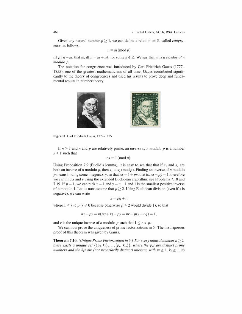
468 7 Partial Orders, GCDs, RSA, Lattices
Given any natural number p ≥ 1, we can define a relation on Z, called congru-ence, as follows.
n≡ m (mod p)
iff p | n−m; that is, iff n = m+ pk, for some k ∈ Z. We say that m is a residue of nmodulo p.
The notation for congruence was introduced by Carl Friedrich Gauss (1777–1855), one of the greatest mathematicians of all time. Gauss contributed signifi-cantly to the theory of congruences and used his results to prove deep and funda-mental results in number theory.
Fig. 7.11 Carl Friedrich Gauss, 1777–1855
If n ≥ 1 and n and p are relatively prime, an inverse of n modulo p is a numbers≥ 1 such that
ns≡ 1 (mod p).
Using Proposition 7.9 (Euclid’s lemma), it is easy to see that that if s1 and s2 areboth an inverse of n modulo p, then s1 ≡ s2 (mod p). Finding an inverse of n modulop means finding some integers x,y, so that nx= 1+ py, that is, nx− py= 1, thereforewe can find x and y using the extended Euclidean algorithm; see Problems 7.18 and7.19. If p = 1, we can pick x = 1 and y = n−1 and 1 is the smallest positive inverseof n modulo 1. Let us now assume that p≥ 2. Using Euclidean division (even if x isnegative), we can write
x = pq+ r,
where 1≤ r < p (r 6= 0 because otherwise p≥ 2 would divide 1), so that
nx− py = n(pq+ r)− py = nr− p(y−nq) = 1,
and r is the unique inverse of n modulo p such that 1≤ r < p.We can now prove the uniqueness of prime factorizations in N. The first rigorous
proof of this theorem was given by Gauss.
Theorem 7.10. (Unique Prime Factorization in N) For every natural number a≥ 2,there exists a unique set 〈p1,k1〉, . . . ,〈pm,km〉, where the pis are distinct primenumbers and the kis are (not necessarily distinct) integers, with m ≥ 1, ki ≥ 1, so
7.4 Unique Prime Factorization in Z and GCDs 469
thata = pk1
1 · · · pkmm .
Proof . The existence of such a factorization has already been proved in Theorem7.5.
Let us now prove uniqueness. Assume that
a = pk11 · · · pkm
m and a = qh11 · · ·qhn
n .
Thus, we havepk1
1 · · · pkmm = qh1
1 · · ·qhnn .
We prove that m= n, pi = qi, and hi = ki, for all i, with 1≤ i≤ n. The proof proceedsby induction on h1 + · · ·+hn.
If h1 + · · ·+hn = 1, then n = 1 and h1 = 1. Then,
pk11 · · · pkm
m = q1,
and because q1 and the pi are prime numbers, we must have m = 1 and p1 = q1 (aprime is only divisible by 1 or itself).
If h1 + · · ·+hn ≥ 2, because h1 ≥ 1, we have
pk11 · · · pkm
m = q1q,
withq = qh1−1
1 · · ·qhnn ,
where (h1−1)+ · · ·+hn ≥ 1 (and qh1−11 = 1 if h1 = 1). Now, if q1 is not equal to any
of the pi, by a previous remark, q1 and pi are relatively prime, and by Proposition7.10, q1 and pk1
1 · · · pkmm are relatively prime. But this contradicts the fact that q1
divides pk11 · · · pkm
m . Thus, q1 is equal to one of the pi. Without loss of generality, wecan assume that q1 = p1. Then, as q1 6= 0, we get
pk1−11 · · · pkm
m = qh1−11 · · ·qhn
n ,
where pk1−11 = 1 if k1 = 1, and qh1−1
1 = 1 if h1 = 1. Now, (h1− 1) + · · ·+ hn <h1 + · · ·+ hn, and we can apply the induction hypothesis to conclude that m = n,pi = qi and hi = ki, with 1≤ i≤ n. ut
Theorem 7.10 is a basic but very important result of number theory and it hasmany applications. It also reveals the importance of the primes as the building blocksof all numbers.
Remark: Theorem 7.10 also applies to any nonzero integer a ∈ Z−−1,+1, byadding a suitable sign in front of the prime factorization. That is, we have a uniqueprime factorization of the form
a =±pk11 · · · pkm
m .

470 7 Partial Orders, GCDs, RSA, Lattices
Theorem 7.10 shows that Z is a unique factorization domain, for short, a UFD.Such rings play an important role because every nonzero element that is not a unit(i.e., which is not invertible) has a unique factorization (up to some unit factor) intoso-called irreducible elements which generalize the primes.
Readers who would like to learn more about number theory are strongly advisedto read Silverman’s delightful and very “friendly” introductory text [15]. Anotherexcellent but more advanced text is Davenport [3] and an even more comprehensivebook (and a classic) is Niven, Zuckerman, and Montgomery [12]. For those inter-ested in the history of number theory (up to Gauss), we highly recommend Weil[17], a fascinating book (but no easy reading).
In the next section, we give a beautiful application of the pigeonhole principle tonumber theory due to Dirichlet (1805–1949).
7.5 Dirichlet’s Diophantine Approximation Theorem
The pigeonhole principle (see Section 3.11) was apparently first stated explicitly byDirichlet in 1834. Dirichlet used the pigeonhole principle (under the name Schub-fachschluß) to prove a fundamental theorem about the approximation of irrationalnumbers by fractions (rational numbers). The proof is such a beautiful illustration
Fig. 7.12 Johan Peter Gustav Lejeune Dirichlet, 1805–1859
of the use of the pigeonhole principle that we can’t resist presenting it. Recall that areal number α ∈ R is irrational iff it cannot be written as a fraction p/q ∈Q.
Theorem 7.11. (Dirichlet) For every positive irrational number α > 0, there areinfinitely many pairs of positive integers, (x,y), such that gcd(x,y) = 1 and
|x− yα|< 1y.
Proof . Pick any positive integer m such that m≥ 1/α , and consider the numbers
0, α, 2α, 3α, · · · ,mα.

7.5 Dirichlet’s Diophantine Approximation Theorem 471
We can write each number in the above list as the sum of a whole number (a naturalnumber) and a decimal real part, between 0 and 1, say
0 = N0 +F0
α = N1 +F1
2α = N2 +F2
3α = N3 +F3
...mα = Nm +Fm,
with N0 = F0 = 0, Ni ∈ N, and 0 ≤ Fi < 1, for i = 1, . . . ,m. Observe that there arem+1 numbers F0, . . . ,Fm. Consider the m “boxes” consisting of the intervals
t ∈ R∣∣∣∣ i
m≤ t <
i+1m
, 0≤ i≤ m−1.
There are m+1 numbers Fi, and only m intervals, thus by the pigeonhole principle,two of these numbers must be in the same interval, say Fi and Fj, for i < j. As
im≤ Fi,Fj <
i+1m
,
we must have|Fi−Fj|<
1m
and because iα = Ni +Fi and jα = N j +Fj, we conclude that
|iα−Ni− ( jα−N j)|<1m
;
that is,
|N j−Ni− ( j− i)α|< 1m.
Note that 1≤ j− i≤ m and so, if N j−Ni = 0, then
α <1
( j− i)m≤ 1
m,
which contradicts the hypothesis m ≥ 1/α . Therefore, x = N j −Ni > 0 and y =j− i > 0 are positive integers such that y≤ m and
|x− yα|< 1m.
If gcd(x,y) = d > 1, then write x = dx′, y = dy′, and divide both sides of the aboveinequality by d to obtain
472 7 Partial Orders, GCDs, RSA, Lattices
|x′− y′α|< 1md
<1m
with gcd(x′,y′) = 1 and y′ < m. In either case, we proved that there exists a pair ofpositive integers (x,y), with y≤ m and gcd(x,y) = 1 such that
|x− yα|< 1m.
However, y≤ m, so we also have
|x− yα|< 1m≤ 1
y,
as desired.Suppose that there are only finitely many pairs (x,y) satisfying gcd(x,y) = 1 and
|x− yα|< 1y.
In this case, there are finitely many values for |x− yα| and thus, the minimal valueof |x− yα| is achieved for some (x0,y0). Furthermore, as α is irrational, we have0 < |x0− y0α|. However, if we pick m large enough, we can find (x,y) such thatgcd(x,y) = 1 and
|x− yα|< 1m
< |x0− y0α|,
contradicting the minimality of |x0−y0α|. Therefore, there are infinitely many pairs(x,y), satisfying the theorem. ut
Note that Theorem 7.11 yields rational approximations for α , because after divi-sion by y, we get ∣∣∣∣xy −α
∣∣∣∣< 1y2 .
For example,355113
= 3.1415929204,
a good approximation ofπ = 3.1415926535 . . .
The fraction10399333102
= 3.1415926530
is even better.
Remark: Actually, Dirichlet proved his approximation theorem for irrational num-bers of the form
√D, where D is a positive integer that is not a perfect square, but
a trivial modification of his proof applies to any (positive) irrational number. Oneshould consult Dirichlet’s original proof in Dirichlet [5], Supplement VIII. This

7.6 Fibonacci and Lucas Numbers; Mersenne Primes 473
book was actually written by R. Dedekind in 1863 based on Dirichlet’s lectures,after Dirichlet’s death. It is considered as one of the most important mathematicsbook of the nineteenth century and it is a model of exposition for its clarity.
Theorem 7.11 only gives a brute-force method for finding x and y, namely, giveny, we pick x to be the integer closest to yα . There are better ways for finding rationalapproximations based on continued fractions; see Silverman [15], Davenport [3], orNiven, Zuckerman, and Montgomery [12].
It should also be noted that Dirichlet made another clever use of the pigeonholeprinciple to prove that the equation (known as Pell’s equation)
x2−Dy2 = 1,
where D is a positive integer that is not a perfect square, has some solution (x,y),where x and y are positive integers. Such equations had been considered by Fermataround the 1640s and long before that by the Indian mathematicians, Brahmagupta(598–670) and Bhaskaracharya (1114–1185). Surprisingly, the solution with thesmallest x can be very large. For example, the smallest (positive) solution of
x2−61y2 = 1
is (x1,y1) = (1766319049,226153980).It can also be shown that Pell’s equation has infinitely many solutions (in pos-
itive integers) and that these solutions can be expressed in terms of the smallestsolution. For more on Pell’s equation, see Silverman [15] and Niven, Zuckerman,and Montgomery [12].
We now take a well-deserved break from partial orders and take a look at Fi-bonacci and Lucas numbers.
7.6 Fibonacci and Lucas Numbers; Mersenne Primes
We have encountered the Fibonacci numbers (after Leonardo Fibonacci, also knownas Leonardo of Pisa, 1170–1250) in Section 3.3. These numbers show up unex-pectedly in many places, including algorithm design and analysis, for example, Fi-bonacci heaps. The Lucas numbers (after Edouard Lucas, 1842–1891) are closelyrelated to the Fibonacci numbers. Both arise as special instances of the recurrencerelation
un+2 = un+1 +un, n≥ 0,
where u0 and u1 are some given initial values.The Fibonacci sequence (Fn) arises for u0 = 0 and u1 = 1 and the Lucas sequence
(Ln) for u0 = 2 and u1 = 1. These two sequences turn out to be intimately related andthey satisfy many remarkable identities. The Lucas numbers play a role in testingfor primality of certain kinds of numbers of the form 2p− 1, where p is a prime,
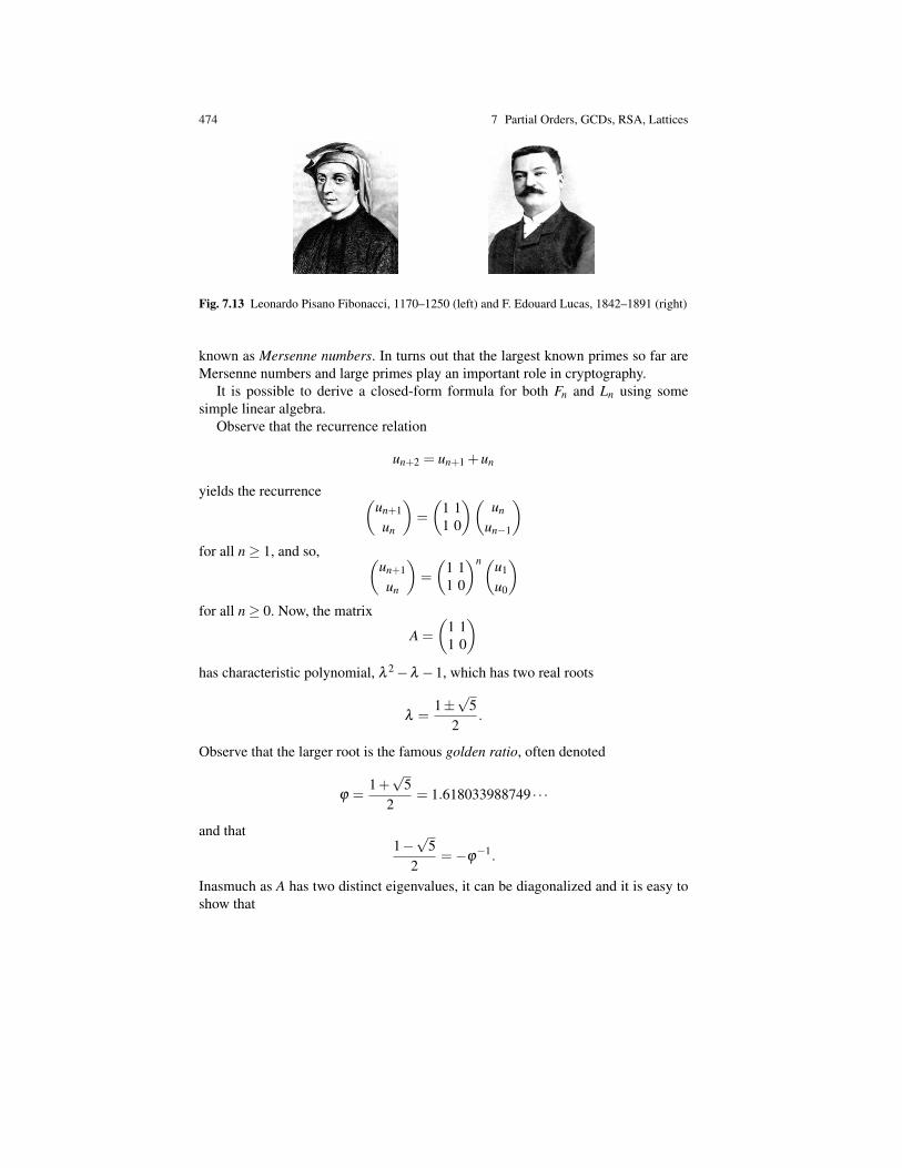
474 7 Partial Orders, GCDs, RSA, Lattices
Fig. 7.13 Leonardo Pisano Fibonacci, 1170–1250 (left) and F. Edouard Lucas, 1842–1891 (right)
known as Mersenne numbers. In turns out that the largest known primes so far areMersenne numbers and large primes play an important role in cryptography.
It is possible to derive a closed-form formula for both Fn and Ln using somesimple linear algebra.
Observe that the recurrence relation
un+2 = un+1 +un
yields the recurrence (un+1
un
)=
(1 11 0
)(un
un−1
)for all n≥ 1, and so, (
un+1
un
)=
(1 11 0
)n(u1
u0
)for all n≥ 0. Now, the matrix
A =
(1 11 0
)has characteristic polynomial, λ 2−λ −1, which has two real roots
λ =1±√
52
.
Observe that the larger root is the famous golden ratio, often denoted
ϕ =1+√
52
= 1.618033988749 · · ·
and that1−√
52
=−ϕ−1.
Inasmuch as A has two distinct eigenvalues, it can be diagonalized and it is easy toshow that

7.6 Fibonacci and Lucas Numbers; Mersenne Primes 475
A =
(1 11 0
)=
1√5
(ϕ −ϕ−1
1 1
)(ϕ 00 −ϕ−1
)(1 ϕ−1
−1 ϕ
).
It follows that (un+1
un
)=
1√5
(ϕ −ϕ−1
1 1
)((ϕ−1u0 +u1)ϕ
n
(ϕu0−u1)(−ϕ−1)n
),
and so,
un =1√5
((ϕ−1u0 +u1)ϕ
n +(ϕu0−u1)(−ϕ−1)n),
for all n≥ 0.For the Fibonacci sequence, u0 = 0 and u1 = 1, so
Fn =1√5
(ϕ
n− (−ϕ−1)n)= 1√
5
[(1+√
52
)n
−(
1−√
52
)n],
a formula established by Jacques Binet (1786–1856) in 1843 and already known toEuler, Daniel Bernoulli, and de Moivre. Because
ϕ−1√
5=
√5−1
2√
5<
12,
we see that Fn is the closest integer to ϕn/√
5 and that
Fn =
⌊ϕn√
5+
12
⌋.
It is also easy to see thatFn+1 = ϕFn +(−ϕ
−1)n,
which shows that the ratio Fn+1/Fn approaches ϕ as n goes to infinity.For the Lucas sequence, u0 = 2 and u1 = 1, so
ϕ−1u0 +u1 = 2
(√
5−1)2
+1 =√
5,
ϕu0−u1 = 2(1+√
5)2
−1 =√
5
and we get
Ln = ϕn +(−ϕ
−1)n =
(1+√
52
)n
+
(1−√
52
)n
.
Because
ϕ−1 =
√5−12
< 0.62

476 7 Partial Orders, GCDs, RSA, Lattices
it follows that Ln is the closest integer to ϕn.When u0 = u1, because ϕ−ϕ−1 = 1, we get
un =u0√
5
(ϕ
n+1− (−ϕ−1)n+1);
that is,un = u0Fn+1.
Therefore, from now on, we assume that u0 6= u1. It is easy to prove the followingby induction.
Proposition 7.11. The following identities hold.
F20 +F2
1 + · · ·+F2n = FnFn+1
F0 +F1 + · · ·+Fn = Fn+2−1F2 +F4 + · · ·+F2n = F2n+1−1
F1 +F3 + · · ·+F2n+1 = F2n+2n
∑k=0
kFk = nFn+2−Fn+3 +2
for all n≥ 0 (with the third sum interpreted as F0 for n = 0).
Following Knuth (see [7]), the third and fourth identities yield the identity
F(n mod 2)+2 + · · ·+Fn−2 +Fn = Fn+1−1,
for all n≥ 2.The above can be used to prove the Zeckendorf representation of the natural
numbers (see Knuth [7], Chapter 6).
Proposition 7.12. (Zeckendorf’s Representation) Every natural number n ∈ N withn > 0, has a unique representation of the form
n = Fk1 +Fk2 + · · ·+Fkr ,
with ki ≥ ki+1 +2 for i = 1, . . . ,r−1 and kr ≥ 2.
For example,
30 = 21+8+1= F8 +F6 +F2
and
1000000 = 832040+121393+46368+144+55= F30 +F26 +F24 +F12 +F10.

7.6 Fibonacci and Lucas Numbers; Mersenne Primes 477
The fact thatFn+1 = ϕFn +(−ϕ
−1)n
and the Zeckendorf representation lead to an amusing method for converting be-tween kilometers and miles (see [7], Section 6.6). Indeed, ϕ is nearly the number ofkilometers in a mile (the exact number is 1.609344 and ϕ = 1.618033). It followsthat a distance of Fn+1 kilometers is very nearly a distance of Fn miles,
Thus, to convert a distance d expressed in kilometers into a distance expressedin miles, first find the Zeckendorf representation of d and then shift each Fki in thisrepresentation to Fki−1. For example,
30 = 21+8+1 = F8 +F6 +F2
so the corresponding distance in miles is
F7 +F6 +F1 = 13+5+1 = 19.
The “exact” distance in miles is 18.64 miles.We can prove two simple formulas for obtaining the Lucas numbers from the
Fibonacci numbers and vice-versa:
Proposition 7.13. The following identities hold:
Ln = Fn−1 +Fn+1
5Fn = Ln−1 +Ln+1,
for all n≥ 1.
The Fibonacci sequence begins with0,1,1,2,3,5,8,13,21,34,55,89,144,233,377,610
and the Lucas sequence begins with2,1,3,4,7,11,18,29,47,76,123,199,322,521,843,1364.Notice that Ln = Fn−1 +Fn+1 is equivalent to
2Fn+1 = Fn +Ln.
It can also be shown thatF2n = FnLn,
for all n≥ 1.The proof proceeds by induction but one finds that it is necessary to prove an
auxiliary fact.
Proposition 7.14. For any fixed k ≥ 1 and all n≥ 0, we have
Fn+k = FkFn+1 +Fk−1Fn.
The reader can also prove that

478 7 Partial Orders, GCDs, RSA, Lattices
LnLn+2 = L2n+1 +5(−1)n
L2n = L2n−2(−1)n
L2n+1 = LnLn+1− (−1)n
L2n = 5F2
n +4(−1)n.
Using the matrix representation derived earlier, the following can be shown.
Proposition 7.15. The sequence given by the recurrence
un+2 = un+1 +un
satisfies the equation:
un+1un−1−u2n = (−1)n−1(u2
0 +u0u1−u21).
For the Fibonacci sequence, where u0 = 0 and u1 = 1, we get the Cassini identity(after Jean-Dominique Cassini, also known as Giovanni Domenico Cassini, 1625–1712),
Fn+1Fn−1−F2n = (−1)n, n≥ 1.
The above identity is a special case of Catalan’s identity,
Fn+rFn−r−F2n = (−1)n−r+1F2
r , n≥ r,
due to Eugene Catalan (1814–1894).
Fig. 7.14 Jean-Dominique Cassini, 1748–1845 (left) and Eugene Charles Catalan, 1814–1984(right)
For the Lucas numbers, where u0 = 2 and u1 = 1 we get
Ln+1Ln−1−L2n = 5(−1)n−1, n≥ 1.
In general, we have
ukun+1 +uk−1un = u1un+k +u0un+k−1,
for all k ≥ 1 and all n≥ 0.
7.6 Fibonacci and Lucas Numbers; Mersenne Primes 479
For the Fibonacci sequence, where u0 = 0 and u1 = 1, we just re-proved theidentity
Fn+k = FkFn+1 +Fk−1Fn.
For the Lucas sequence, where u0 = 2 and u1 = 1, we get
LkLn+1 +Lk−1Ln = Ln+k +2Ln+k−1
= Ln+k +Ln+k−1 +Ln+k−1
= Ln+k+1 +Ln+k−1
= 5Fn+k;
that is,LkLn+1 +Lk−1Ln = Ln+k+1 +Ln+k−1 = 5Fn+k,
for all k ≥ 1 and all n≥ 0.The identity
Fn+k = FkFn+1 +Fk−1Fn
plays a key role in the proof of various divisibility properties of the Fibonacci num-bers. Here are two such properties.
Proposition 7.16. The following properties hold.
1. Fn divides Fmn, for all m,n≥ 1.2. gcd(Fm,Fn) = Fgcd(m,n), for all m,n≥ 1.
An interesting consequence of this divisibility property is that if Fn is a primeand n > 4, then n must be a prime. Indeed, if n≥ 5 and n is not prime, then n = pqfor some integers p,q (possibly equal) with p≥ 2 and q≥ 3, so Fq divides Fpq = Fnand becaue q≥ 3, Fq ≥ 2 and Fn is not prime. For n = 4, F4 = 3 is prime. However,there are prime numbers n ≥ 5 such that Fn is not prime, for example, n = 19, asF19 = 4181 = 37×113 is not prime.
The gcd identity can also be used to prove that for all m,n with 2 < n < m, if Fndivides Fm, then n divides m, which provides a converse of our earlier divisibilityproperty.
The formulae
2Fm+n = FmLn +FnLm
2Lm+n = LmLn +5FmFn
are also easily established using the explicit formulae for Fn and Ln in terms of ϕ
and ϕ−1.The Fibonacci sequence and the Lucas sequence contain primes but it is unknown
whether they contain infinitely many primes. Here are some facts about Fibonacciand Lucas primes taken from The Little Book of Bigger Primes , by Paulo Riben-boim [13].
As we proved earlier, if Fn is a prime and n 6= 4, then n must be a prime but theconverse is false. For example,

480 7 Partial Orders, GCDs, RSA, Lattices
F3,F4,F5,F7,F11,F13,F17,F23
are prime but F19 = 4181 = 37× 113 is not a prime. One of the largest prime Fi-bonacci numbers is F81839. This number has 17,103 digits. Concerning the Lucasnumbers, we prove shortly that if Ln is an odd prime and n is not a power of 2, thenn is a prime. Again, the converse is false. For example,
L0,L2,L4,L5,L7,L8,L11,L13,L16,L17,L19,L31
are prime but L23 = 64079 = 139×461 is not a prime. Similarly, L32 = 4870847 =1087×4481 is not prime. One of the largest Lucas primes is L51169.
Generally, divisibility properties of the Lucas numbers are not easy to prove be-cause there is no simple formula for Lm+n in terms of other Lks. Nevertheless, wecan prove that if n,k ≥ 1 and k is odd, then Ln divides Lkn. This is not necessarilytrue if k is even. For example, L4 = 7 and L8 = 47 are prime. The trick is that whenk is odd, the binomial expansion of Lk
n = (ϕn +(−ϕ−1)n)k has an even number ofterms and these terms can be paired up. Indeed, if k is odd, say k = 2h+1, we havethe formula
L2h+1n = L(2h+1)n +
(2h+1
1
)(−1)nL(2h−1)n +
(2h+1
2
)(−1)2nL(2h−3)n + · · ·
+
(2h+1
h
)(−1)hnLn.
By induction on h, we see that Ln divides L(2h+1)n for all h ≥ 0. Consequently, ifn ≥ 2 is not prime and not a power of 2, then either n = 2iq for some odd integer,q≥ 3, and some i≥ 1 and thus, L2i ≥ 3 divides Ln, or n = pq for some odd integers(possibly equal), p≥ 3 and q≥ 3, and so, Lp ≥ 4 (and Lq ≥ 4) divides Ln. Therefore,if Ln is an odd prime (so n 6= 1, because L1 = 1) then either n is a power of 2 or n isprime.
Remark: When k is even, say k = 2h, the “middle term,”(2h
h
)(−1)hn, in the bino-
mial expansion of L2hn = (ϕn +(−ϕ−1)n)2h stands alone, so we get
L2hn = L2hn +
(2h1
)(−1)nL(2h−2)n +
(2h2
)(−1)2nL(2h−4)n + · · ·
+
(2h
h−1
)(−1)(h−1)nL2n +
(2hh
)(−1)hn.
Unfortunately, the above formula seems of little use to prove that L2hn is divisibleby Ln. Note that the last term is always even inasmuch as(
2hh
)=
(2h)!h!h!
=2hh
(2h−1)!(h−1)!h!
= 2(
2h−1h
).
It should also be noted that not every sequence (un) given by the recurrence

7.6 Fibonacci and Lucas Numbers; Mersenne Primes 481
un+2 = un+1 +un
and with gcd(u0,u1) = 1 contains a prime number. According to Ribenboim [13],Graham found an example in 1964 but it turned out to be incorrect. Later, Knuthgave correct sequences (see Concrete Mathematics [7], Chapter 6), one of whichbegan with
u0 = 62638280004239857u1 = 49463435743205655.
We just studied some properties of the sequences arising from the recurrencerelation
un+2 = un+1 +un.
Lucas investigated the properties of the more general recurrence relation
un+2 = Pun+1−Qun,
where P,Q ∈ Z are any integers with P2−4Q 6= 0, in two seminal papers publishedin 1878.
We can prove some of the basic results about these Lucas sequences quite easilyusing the matrix method that we used before. The recurrence relation
un+2 = Pun+1−Qun
yields the recurrence (un+1
un
)=
(P −Q1 0
)(un
un−1
)for all n≥ 1, and so, (
un+1
un
)=
(P −Q1 0
)n(u1
u0
)for all n≥ 0. The matrix
A =
(P −Q1 0
)has the characteristic polynomial −(P− λ )λ +Q = λ 2−Pλ +Q, which has thediscriminant D = P2− 4Q. If we assume that P2− 4Q 6= 0, the polynomial λ 2−Pλ +Q has two distinct roots:
α =P+√
D2
, β =P−√
D2
.
Obviously,
482 7 Partial Orders, GCDs, RSA, Lattices
α +β = P
αβ = Q
α−β =√
D.
The matrix A can be diagonalized as
A =
(P −Q1 0
)=
1α−β
(α β
1 1
)(α 00 β
)(1 −β
−1 α
).
Thus, we get (un+1
un
)=
1α−β
(α β
1 1
)((−βu0 +u1)α
n
(αu0−u1)β n
)and so,
un =1
α−β
((−βu0 +u1)α
n +(αu0−u1)βn).
Actually, the above formula holds for n = 0 only if α 6= 0 and β 6= 0, that is, iffQ 6= 0. If Q = 0, then either α = 0 or β = 0, in which case the formula still holds ifwe assume that 00 = 1.
For u0 = 0 and u1 = 1, we get a generalization of the Fibonacci numbers,
Un =αn−β n
α−β
and for u0 = 2 and u1 = P, because
−βu0 +u1 =−2β +P =−2β +α +β = α−β
andαu0−u1 = 2α−P = 2α− (α +β ) = α−β ,
we get a generalization of the Lucas numbers,
Vn = αn +β
n.
The orginal Fibonacci and Lucas numbers correspond to P = 1 and Q =−1. Thevectors
(01
)and
(2P
)are linearly independent, therefore every sequence arising from
the recurrence relationun+2 = Pun+1−Qun
is a unique linear combination of the sequences (Un) and (Vn).It is possible to prove the following generalization of the Cassini identity.
Proposition 7.17. The sequence defined by the recurrence
un+2 = Pun+1−Qun
(with P2−4Q 6= 0) satisfies the identity:
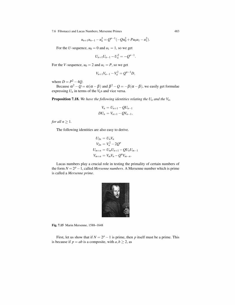
7.6 Fibonacci and Lucas Numbers; Mersenne Primes 483
un+1un−1−u2n = Qn−1(−Qu2
0 +Pu0u1−u21).
For the U-sequence, u0 = 0 and u1 = 1, so we get
Un+1Un−1−U2n =−Qn−1.
For the V -sequence, u0 = 2 and u1 = P, so we get
Vn+1Vn−1−V 2n = Qn−1D,
where D = P2−4Q.Because α2−Q = α(α−β ) and β 2−Q =−β (α−β ), we easily get formulae
expressing Un in terms of the Vks and vice versa.
Proposition 7.18. We have the following identities relating the Un and the Vn,
Vn = Un+1−QUn−1
DUn = Vn+1−QVn−1,
for all n≥ 1.
The following identities are also easy to derive.
U2n = UnVn
V2n = V 2n −2Qn
Um+n = UmUn+1−QUnUm−1
Vm+n = VmVn−QnVm−n.
Lucas numbers play a crucial role in testing the primality of certain numbers ofthe form N = 2p−1, called Mersenne numbers. A Mersenne number which is primeis called a Mersenne prime.
Fig. 7.15 Marin Mersenne, 1588–1648
First, let us show that if N = 2p−1 is prime, then p itself must be a prime. Thisis because if p = ab is a composite, with a,b≥ 2, as

484 7 Partial Orders, GCDs, RSA, Lattices
2p−1 = 2ab−1 = (2a−1)(1+2a +22a + · · ·+2(b−1)a),
then 2a−1 > 1 divides 2p−1, a contradiction.For p = 2,3,5,7 we see that 3 = 22− 1, 7 = 23− 1, 31 = 25− 1, 127 = 27− 1
are indeed prime.However, the condition that the exponent p be prime is not sufficient for N =
2p−1 to be prime, because for p= 11, we have 211−1= 2047= 23×89. Mersenne(1588–1648) stated in 1644 that N = 2p−1 is prime when
p = 2,3,5,7,13,17,19,31,67,127,257.
Mersenne was wrong about p = 67 and p = 257, and he missed p = 61,89, and 107.Euler showed that 231−1 was indeed prime in 1772 and at that time, it was knownthat 2p−1 is indeed prime for p = 2,3,5,7,13,17,19,31.
Then came Lucas. In 1876, Lucas, proved that 2127− 1 was prime. Lucas cameup with a method for testing whether a Mersenne number is prime, later rigorouslyproved correct by Lehmer, and known as the Lucas–Lehmer test. This test does notrequire the actual computation of N = 2p−1 but it requires an efficient method forsquaring large numbers (less that N) and a way of computing the residue modulo2p−1 just using p.
A version of the Lucas–Lehmer test uses the Lucas sequence given by the recur-rence
Vn+2 = 2Vn+1 +2Vn,
starting from V0 = V1 = 2. This corresponds to P = 2 and Q = −2. In this case,D = 12 and it is easy to see that α = 1+
√3, β = 1−
√3, so
Vn = (1+√
3)n +(1−√
3)n.
This sequence starts with2,2,8,20,56, . . . .
Here is the first version of the Lucas–Lehmer test for primality of a Mersenne num-ber.
Fig. 7.16 Derrick Henry Lehmer, 1905–1991

7.6 Fibonacci and Lucas Numbers; Mersenne Primes 485
Theorem 7.12. Lucas–Lehmer test (Version 1) The number N = 2p−1 is prime forany odd prime p iff N divides V2p−1 .
A proof of the Lucas–Lehmer test can be found in The Little Book of BiggerPrimes [13]. Shorter proofs exist and are available on the Web but they requiresome knowledge of algebraic number theory. The most accessible proof that we areaware of (it only uses the quadratic reciprocity law) is given in Volume 2 of Knuth[8]; see Section 4.5.4. Note that the test does not apply to p = 2 because 3 = 22−1does not divide V2 = 8 but that’s not a problem.
The numbers V2p−1 get large very quickly but if we observe that
V2n =V 2n −2(−2)n,
we may want to consider the sequence Sn, given by
Sn+1 = S2n−2,
starting with S0 = 4. This sequence starts with
4,14,194,37643,1416317954, . . . .
Then, it turns out thatV2k = Sk−122k−1
,
for all k ≥ 1. It is also easy to see that
Sk = (2+√
3)2k+(2−
√3)2k
.
Now, N = 2p−1 is prime iff N divides V2p−1 iff N = 2p−1 divides Sp−222p−2iff
N divides Sp−2 (because if N divides 22p−2, then N is not prime).
Thus, we obtain an improved version of the Lucas–Lehmer test for primality ofa Mersenne number.
Theorem 7.13. Lucas–Lehmer test (Version 2) The number, N = 2p−1, is prime forany odd prime p iff
Sp−2 ≡ 0 (mod N).
The test does not apply to p = 2 because 3 = 22− 1 does not divide S0 = 4 butthat’s not a problem.
The above test can be performed by computing a sequence of residues mod N,using the recurrence Sn+1 = S2
n−2, starting from 4.As of January 2009, only 46 Mersenne primes were known. The largest one was
found in August 2008 by mathematicians at UCLA. This is
M46 = 243112609−1,
and it has 12,978,189 digits. It is an open problem whether there are infinitely manyMersenne primes.
486 7 Partial Orders, GCDs, RSA, Lattices
Going back to the second version of the Lucas–Lehmer test, because we arecomputing the sequence of Sks modulo N, the squares being computed never exceedN2 = 22p. There is also a clever way of computing n mod 2p− 1 without actuallyperforming divisions if we express n in binary. This is because
n≡ (n mod 2p)+ bn/2pc (mod 2p−1).
But now, if n is expressed in binary, (n mod 2p) consists of the p rightmost(least significant) bits of n and bn/2pc consists of the bits remaining as the headof the string obtained by deleting the rightmost p bits of n. Thus, we can computethe remainder modulo 2p− 1 by repeating this process until at most p bits remain.Observe that if n is a multiple of 2p−1, the algorithm will produce 2p−1 in binaryas opposed to 0 but this exception can be handled easily. For example,
916 mod 25−1 = 11100101002 (mod 25−1)= 101002 +111002 (mod 25−1)= 1100002 (mod 25−1)= 100002 +12 (mod 25−1)= 100012 (mod 25−1)= 100012
= 17.
The Lucas–Lehmer test applied to N = 127 = 27−1 yields the following steps,if we denote Sk mod 2p−1 by rk.r0 = 4,r1 = 42−2 = 14 (mod 127); that is, r1 = 14.r2 = 142−2 = 194 (mod 127); that is, r2 = 67.r3 = 672−2 = 4487 (mod 127); that is, r3 = 42.r4 = 422−2 = 1762 (mod 127); that is, r4 = 111.r5 = 1112−2 = 12319 (mod 127); that is, r5 = 0.
As r5 = 0, the Lucas–Lehmer test confirms that N = 127= 27−1 is indeed prime.
7.7 Public Key Cryptography; The RSA System
Ever since written communication was used, people have been interested in tryingto conceal the content of their messages from their adversaries. This has led to thedevelopment of techniques of secret communication, a science known as cryptogra-phy.
The basic situation is that one party, A, say Albert, wants to send a messageto another party, J, say Julia. However, there is a danger that some ill-intentionedthird party, Machiavelli, may intercept the message and learn things that he is not
7.7 Public Key Cryptography; The RSA System 487
supposed to know about and as a result, do evil things. The original message, un-derstandable to all parties, is known as the plain text. To protect the content of themessage, Albert encrypts his message. When Julia receives the encrypted message,she must decrypt it in order to be able to read it. Both Albert and Julia share someinformation that Machiavelli does not have, a key. Without a key, Machiavelli, isincapable of decrypting the message and thus, to do harm.
There are many schemes for generating keys to encrypt and decrypt messages.We are going to describe a method involving public and private keys known asthe RSA Cryptosystem, named after its inventors, Ronald Rivest, Adi Shamir, andLeonard Adleman (1978), based on ideas by Diffie and Hellman (1976). We highlyrecommend reading the orginal paper by Rivest, Shamir, and Adleman [14]. It isbeautifully written and easy to follow. A very clear, but concise exposition can alsobe found in Koblitz [9]. An encyclopedic coverage of cryptography can be found inMenezes, van Oorschot, and Vanstone’s Handbook [11].
The RSA system is widely used in practice, for example in SSL (Secure SocketLayer), which in turn is used in https (secure http). Any time you visit a “secure site”on the Internet (to read e-mail or to order merchandise), your computer generates apublic key and a private key for you and uses them to make sure that your credit cardnumber and other personal data remain secret. Interestingly, although one mightthink that the mathematics behind such a scheme is very advanced and complicated,this is not so. In fact, little more than the material of Section 7.4 is needed. Therefore,in this section, we are going to explain the basics of RSA.
The first step is to convert the plain text of characters into an integer. This canbe done easily by assigning distinct integers to the distinct characters, for example,by converting each character to its ASCII code. From now on, we assume that thisconversion has been performed.
The next and more subtle step is to use modular arithmetic. We pick a (large)positive integer m and perform arithmetic modulo m. Let us explain this step inmore detail.
Recall that for all a,b∈Z, we write a≡ b(mod m) iff a−b= km, for some k∈Z,and we say that a and b are congruent modulo m. We already know that congruenceis an equivalence relation but it also satisfies the following properties.
Proposition 7.19. For any positive integer m, for all a1,a2,b1,b2 ∈ Z, the followingproperties hold. If a1 ≡ b1 (mod m) and a2 ≡ b2 (mod m), then
(1) a1 +a2 ≡ b1 +b2 (mod m).(2) a1−a2 ≡ b1−b2 (mod m).(3) a1a2 ≡ b1b2 (mod m).
Proof . We only check (3), leaving (1) and (2) as easy exercises. Because a1 ≡b1 (mod m) and a2 ≡ b2 (mod m), we have a1 = b1 + k1m and a2 = b2 + k2m, forsome k1,k2 ∈ Z, and so
a1a2 = (b1 + k1m)(b2 + k2m) = b1b2 +(b1k2 + k1b2 + k1mk2)m,

488 7 Partial Orders, GCDs, RSA, Lattices
which means that a1a2 ≡ b1b2 (mod m). A more elegant proof consists in observingthat
a1a2−b1b2 = a1(a2−b2)+(a1−b1)b2
= (a1k2 + k1b2)m,
as claimed. ut
Proposition 7.19 allows us to define addition, subtraction, and multiplication onequivalence classes modulo m. If we denote by Z/mZ the set of equivalence classesmodulo m and if we write a for the equivalence class of a, then we define
a+b = a+b
a−b = a−b
ab = ab.
The above make sense because a+b does not depend on the representatives cho-sen in the equivalence classes a and b, and similarly for a−b and ab. Of course,each equivalence class a contains a unique representative from the set of remainders0,1, . . . ,m−1, modulo m, so the above operations are completely determined bym×m tables. Using the arithmetic operations of Z/mZ is called modular arithmetic.
For an arbitrary m, the set Z/mZ is an algebraic structure known as a ring. Ad-dition and subtraction behave as in Z but multiplication is stranger. For example,when m = 6,
2 ·3 = 03 ·4 = 0,
inasmuch as 2 ·3= 6≡ 0(mod6), and 3 ·4= 12≡ 0(mod6). Therefore, it is not truethat every nonzero element has a multiplicative inverse. However, we know fromSection 7.4 that a nonzero integer a has a multiplicative inverse iff gcd(a,m) = 1(use the Bezout identity). For example,
5 ·5 = 1,
because 5 ·5 = 25≡ 1 (mod 6).As a consequence, when m is a prime number, every nonzero element not divisi-
ble by m has a multiplicative inverse. In this case, Z/mZ is more like Q; it is a finitefield. However, note that in Z/mZ we have
1+1+ · · ·+1︸ ︷︷ ︸m times
= 0
(because m≡ 0 (mod m)), a phenomenom that does not happen in Q (or R).
7.7 Public Key Cryptography; The RSA System 489
The RSA method uses modular arithmetic. One of the main ingredients of publickey cryptography is that one should use an encryption function, f : Z/mZ→Z/mZ,which is easy to compute (i.e., can be computed efficiently) but such that its inversef−1 is practically impossible to compute unless one has special additional informa-tion. Such functions are usually referred to as trapdoor one-way functions. Remark-ably, exponentiation modulo m, that is, the function, x 7→ xe mod m, is a trapdoorone-way function for suitably chosen m and e.
Thus, we claim the following.
(1) Computing xe mod m can be done efficiently .(2) Finding x such that
xe ≡ y (mod m)
with 0 ≤ x,y ≤ m− 1, is hard, unless one has extra information about m. Thefunction that finds an eth root modulo m is sometimes called a discrete loga-rithm.
We explain shortly how to compute xe mod m efficiently using the square andmultiply method also known as repeated squaring.
As to the second claim, actually, no proof has been given yet that this function isa one-way function but, so far, this has not been refuted either.
Now, what’s the trick to make it a trapdoor function?What we do is to pick two distinct large prime numbers, p and q (say over 200
decimal digits), which are “sufficiently random” and we let
m = pq.
Next, we pick a random e, with 1 < e < (p−1)(q−1), relatively prime to(p−1)(q−1).
Because gcd(e,(p− 1)(q− 1)) = 1, we know from the discussion just beforeTheorem 7.10 that there is some d with 1 < d < (p− 1)(q− 1), such that ed ≡1 (mod (p−1)(q−1)).
Then, we claim that to find x such that
xe ≡ y (mod m),
we simply compute yd mod m, and this can be done easily, as we claimed earlier.The reason why the above “works” is that
xed ≡ x (mod m), (∗)
for all x ∈ Z, which we prove later.
Setting up RSAIn, summary to set up RSA for Albert (A) to receive encrypted messages, performthe following steps.
1. Albert generates two distinct large and sufficiently random primes, pA and qA.They are kept secret.
490 7 Partial Orders, GCDs, RSA, Lattices
2. Albert computes mA = pAqA. This number called the modulus will be madepublic.
3. Albert picks at random some eA, with 1 < eA < (pA−1)(qA−1), so thatgcd(eA,(pA−1)(qA−1)) = 1. The number eA is called the encryption key andit will also be public.
4. Albert computes the inverse, dA = e−1A modulo mA, of eA. This number is kept
secret. The pair (dA,mA) is Albert’s private key and dA is called the decryptionkey.
5. Albert publishes the pair (eA,mA) as his public key.
Encrypting a MessageNow, if Julia wants to send a message, x, to Albert, she proceeds as follows. First,she splits x into chunks, x1, . . . ,xk, each of length at most mA−1, if necessary (again,I assume that x has been converted to an integer in a preliminary step). Then shelooks up Albert’s public key (eA,mA) and she computes
yi = EA(xi) = xeAi mod mA,
for i = 1, . . . ,k. Finally, she sends the sequence y1, . . . ,yk to Albert. This encryptedmessage is known as the cyphertext. The function EA is Albert’s encryption function.
Decrypting a MessageIn order to decrypt the message y1, . . . ,yk that Julia sent him, Albert uses his privatekey (dA,mA) to compute each
xi = DA(yi) = ydAi mod mA,
and this yields the sequence x1, . . . ,xk. The function DA is Albert’s decryption func-tion.
Similarly, in order for Julia to receive encrypted messages, she must set her ownpublic key (eJ ,mJ) and private key (dJ ,mJ) by picking two distinct primes pJ andqJ and eJ , as explained earlier.
The beauty of the scheme is that the sender only needs to know the public key ofthe recipient to send a message but an eavesdropper is unable to decrypt the encodedmessage unless he somehow gets his hands on the secret key of the receiver.
Let us give a concrete illustration of the RSA scheme using an example borrowedfrom Silverman [15] (Chapter 18). We write messages using only the 26 upper-caseletters A, B, . . . , Z, encoded as the integers A = 11, B = 12, . . . , Z = 36. It would bemore convenient to have assigned a number to represent a blank space but to keepthings as simple as possible we do not do that.
Say Albert picks the two primes pA = 12553 and qA = 13007, so that mA =pAqA = 163,276,871 and (pA−1)(qA−1) = 163,251,312. Albert also picks eA =79921, relatively prime to (pA − 1)(qA − 1) and then finds the inverse dA, of eAmodulo (pA−1)(qA−1) using the extended Euclidean algorithm (more details aregiven in Section 7.9) which turns out to be dA = 145,604,785. One can check that

7.7 Public Key Cryptography; The RSA System 491
145,604,785 ·79921−71282 ·163,251,312 = 1,
which confirms that dA is indeed the inverse of eA modulo 163,251,312.Now, assume that Albert receives the following message, broken in chunks of at
most nine digits, because mA = 163,276,871 has nine digits.
145387828 47164891 152020614 27279275 35356191.
Albert decrypts the above messages using his private key (dA,mA), where dA =145,604,785, using the repeated squaring method (described in Section 7.9) andfinds that
145387828145,604,785 ≡ 30182523 (mod 163,276,871)
47164891145,604,785 ≡ 26292524 (mod 163,276,871)
152020614145,604,785 ≡ 19291924 (mod 163,276,871)
27279275145,604,785 ≡ 30282531 (mod 163,276,871)
35356191145,604,785 ≡ 122215 (mod 163,276,871)
which yields the message
30182523 26292524 19291924 30282531 122215,
and finally, translating each two-digit numeric code to its corresponding character,to the message
T H O M P S O N I S I N T R O U B L E
or, in more readable format
Thompson is in trouble
It would be instructive to encrypt the decoded message
30182523 26292524 19291924 30282531 122215
using the public key eA = 79921. If everything goes well, we should get our originalmessage
145387828 47164891 152020614 27279275 35356191
back.Let us now explain in more detail how the RSA system works and why it is
correct.

492 7 Partial Orders, GCDs, RSA, Lattices
7.8 Correctness of The RSA System
We begin by proving the correctness of the inversion formula (∗). For this, we needa classical result known as Fermat’s little theorem.
Fig. 7.17 Pierre de Fermat, 1601–1665
This result was first stated by Fermat in 1640 but apparently no proof was pub-lished at the time and the first known proof was given by Leibnitz (1646–1716).This is basically the proof suggested in Problem 7.14. A different proof was givenby Ivory in 1806 and this is the proof that we give here. It has the advantage that itcan be easily generalized to Euler’s version (1760) of Fermat’s little theorem.
Theorem 7.14. (Fermat’s Little Theorem) If p is any prime number, then the follow-ing two equivalent properties hold.
(1) For every integer, a ∈ Z, if a is not divisible by p, then we have
ap−1 ≡ 1 (mod p).
(2) For every integer, a ∈ Z, we have
ap ≡ a (mod p).
Proof . (1) Consider the integers
a, 2a, 3a, . . . ,(p−1)a
and letr1, r2, r3, . . . ,rp−1
be the sequence of remainders of the division of the numbers in the first sequenceby p. Because gcd(a, p) = 1, none of the numbers in the first sequence is divisibleby p, so 1 ≤ ri ≤ p−1, for i = 1, . . . , p−1. We claim that these remainders are all
7.8 Correctness of The RSA System 493
distinct. If not, then say ri = r j, with 1≤ i < j ≤ p−1. But then, because
ai≡ ri (mod p)
anda j ≡ r j (mod p),
we deduce thata j−ai≡ r j− ri (mod p),
and because ri = r j, we get,
a( j− i)≡ 0 (mod p).
This means that p divides a( j− i), but gcd(a, p) = 1 so, by Euclid’s lemma (Propo-sition 7.9), p must divide j− i. However 1≤ j− i < p−1, so we get a contradictionand the remainders are indeed all distinct.
There are p− 1 distinct remainders and they are all nonzero, therefore we musthave
r1,r2, . . . ,rp−1= 1,2, . . . , p−1.Using Property (3) of congruences (see Proposition 7.19), we get
a ·2a ·3a · · ·(p−1)a≡ 1 ·2 ·3 · · ·(p−1) (mod p);
that is,(ap−1−1) · (p−1)!≡ 0 (mod p).
Again, p divides (ap−1−1) · (p−1)!, but because p is relatively prime to (p−1)!,it must divide ap−1−1, as claimed.
(2) If gcd(a, p) = 1, we proved in (1) that
ap−1 ≡ 1 (mod p),
from which we getap ≡ a (mod p),
because a ≡ a (mod p). If a is divisible by p, then a ≡ 0 (mod p), which impliesap ≡ 0 (mod p), and thus, that
ap ≡ a (mod p).
Therefore, (2) holds for all a ∈ Z and we just proved that (1) implies (2). Finally,if (2) holds and if gcd(a, p) = 1, as p divides ap− a = a(ap−1− 1), it must divideap−1−1, which shows that (1) holds and so, (2) implies (1). ut
It is now easy to establish the correctness of RSA.
Proposition 7.20. For any two distinct prime numbers p and q, if e and d are anytwo positive integers such that

494 7 Partial Orders, GCDs, RSA, Lattices
1. 1 < e,d < (p−1)(q−1),2. ed ≡ 1 (mod (p−1)(q−1)),
then for every x ∈ Z we have
xed ≡ x (mod pq).
Proof . Because p and q are two distinct prime numbers, by Euclid’s lemma it isenough to prove that both p and q divide xed − x. We show that xed − x is divisibleby p, the proof of divisibility by q being similar.
By condition (2), we have
ed = 1+(p−1)(q−1)k,
with k ≥ 1, inasmuch as 1 < e,d < (p− 1)(q− 1). Thus, if we write h = (q− 1)k,we have h≥ 1 and
xed− x ≡ x1+(p−1)h− x (mod p)
≡ x((xp−1)h−1) (mod p)
≡ x(xp−1−1)((xp−1)h−1 +(xp−1)h−2 + · · ·+1) (mod p)
≡ (xp− x)((xp−1)h−1 +(xp−1)h−2 + · · ·+1) (mod p)
≡ 0 (mod p),
because xp− x≡ 0 (mod p), by Fermat’s little theorem. ut
Remark: Of course, Proposition 7.20 holds if we allow e = d = 1, but this not in-teresting for encryption. The number (p− 1)(q− 1) turns out to be the number ofpositive integers less than pq that are relatively prime to pq. For any arbitrary posi-tive integer, m, the number of positive integers less than m that are relatively primeto m is given by the Euler φ function (or Euler totient), denoted φ (see Problems7.23 and 7.27 or Niven, Zuckerman, and Montgomery [12], Section 2.1, for basicproperties of φ ).
Fermat’s little theorem can be generalized to what is known as Euler’s formula(see Problem 7.23): For every integer a, if gcd(a,m) = 1, then
aφ(m) ≡ 1 (mod m).
Because φ(pq) = (p−1)(q−1), when gcd(x,φ(pq)) = 1, Proposition 7.20 followsfrom Euler’s formula. However, that argument does not show that Proposition 7.20holds when gcd(x,φ(pq))> 1 and a special argument is required in this case.
It can be shown that if we replace pq by a positive integer m that is square-free(does not contain a square factor) and if we assume that e and d are chosen so that1 < e,d < φ(m) and ed ≡ 1 (mod φ(m)), then
xed ≡ x (mod m)
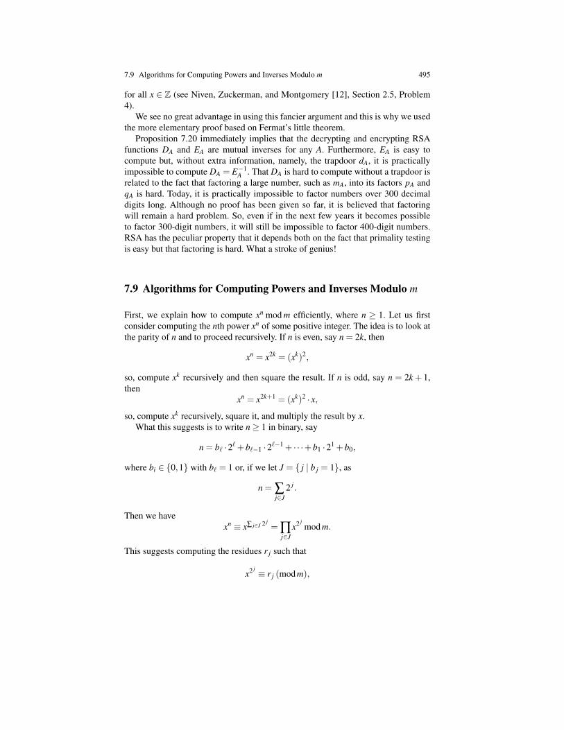
7.9 Algorithms for Computing Powers and Inverses Modulo m 495
for all x ∈ Z (see Niven, Zuckerman, and Montgomery [12], Section 2.5, Problem4).
We see no great advantage in using this fancier argument and this is why we usedthe more elementary proof based on Fermat’s little theorem.
Proposition 7.20 immediately implies that the decrypting and encrypting RSAfunctions DA and EA are mutual inverses for any A. Furthermore, EA is easy tocompute but, without extra information, namely, the trapdoor dA, it is practicallyimpossible to compute DA = E−1
A . That DA is hard to compute without a trapdoor isrelated to the fact that factoring a large number, such as mA, into its factors pA andqA is hard. Today, it is practically impossible to factor numbers over 300 decimaldigits long. Although no proof has been given so far, it is believed that factoringwill remain a hard problem. So, even if in the next few years it becomes possibleto factor 300-digit numbers, it will still be impossible to factor 400-digit numbers.RSA has the peculiar property that it depends both on the fact that primality testingis easy but that factoring is hard. What a stroke of genius!
7.9 Algorithms for Computing Powers and Inverses Modulo m
First, we explain how to compute xn mod m efficiently, where n ≥ 1. Let us firstconsider computing the nth power xn of some positive integer. The idea is to look atthe parity of n and to proceed recursively. If n is even, say n = 2k, then
xn = x2k = (xk)2,
so, compute xk recursively and then square the result. If n is odd, say n = 2k+ 1,then
xn = x2k+1 = (xk)2 · x,so, compute xk recursively, square it, and multiply the result by x.
What this suggests is to write n≥ 1 in binary, say
n = b` ·2`+b`−1 ·2`−1 + · · ·+b1 ·21 +b0,
where bi ∈ 0,1 with b` = 1 or, if we let J = j | b j = 1, as
n = ∑j∈J
2 j.
Then we havexn ≡ x∑ j∈J 2 j
= ∏j∈J
x2 jmod m.
This suggests computing the residues r j such that
x2 j ≡ r j (mod m),

496 7 Partial Orders, GCDs, RSA, Lattices
because then,xn ≡∏
j∈Jr j (mod m),
where we can compute this latter product modulo m two terms at a time.For example, say we want to compute 999179 mod 1763. First, we observe that
179 = 27 +25 +24 +21 +1,
and we compute the powers modulo 1763:
99921 ≡ 143 (mod 1763)
99922 ≡ 1432 ≡ 1056 (mod 1763)
99923 ≡ 10562 ≡ 920 (mod 1763)
99924 ≡ 9202 ≡ 160 (mod 1763)
99925 ≡ 1602 ≡ 918 (mod 1763)
99926 ≡ 9182 ≡ 10 (mod 1763)
99927 ≡ 102 ≡ 100 (mod 1763).
Consequently,
999179 ≡ 999 ·143 ·160 ·918 ·100 (mod 1763)≡ 54 ·160 ·918 ·100 (mod 1763)
≡ 1588 ·918 ·100 (mod 1763)≡ 1546 ·100 (mod 1763)≡ 1219 (mod 1763),
and we find that999179 ≡ 1219 (mod 1763).
Of course, it would be impossible to exponentiate 999179 first and then reduce mod-ulo 1763. As we can see, the number of multiplications needed is O(log2 n), whichis quite good.
The above method can be implemented without actually converting n to base 2. Ifn is even, say n= 2k, then n/2= k and if n is odd, say n= 2k+1, then (n−1)/2= k,so we have a way of dropping the unit digit in the binary expansion of n and shiftingthe remaining digits one place to the right without explicitly computing this binaryexpansion. Here is an algorithm for computing xn mod m, with n ≥ 1, using therepeated squaring method.
An Algorithm to Compute xn mod m Using Repeated Squaring
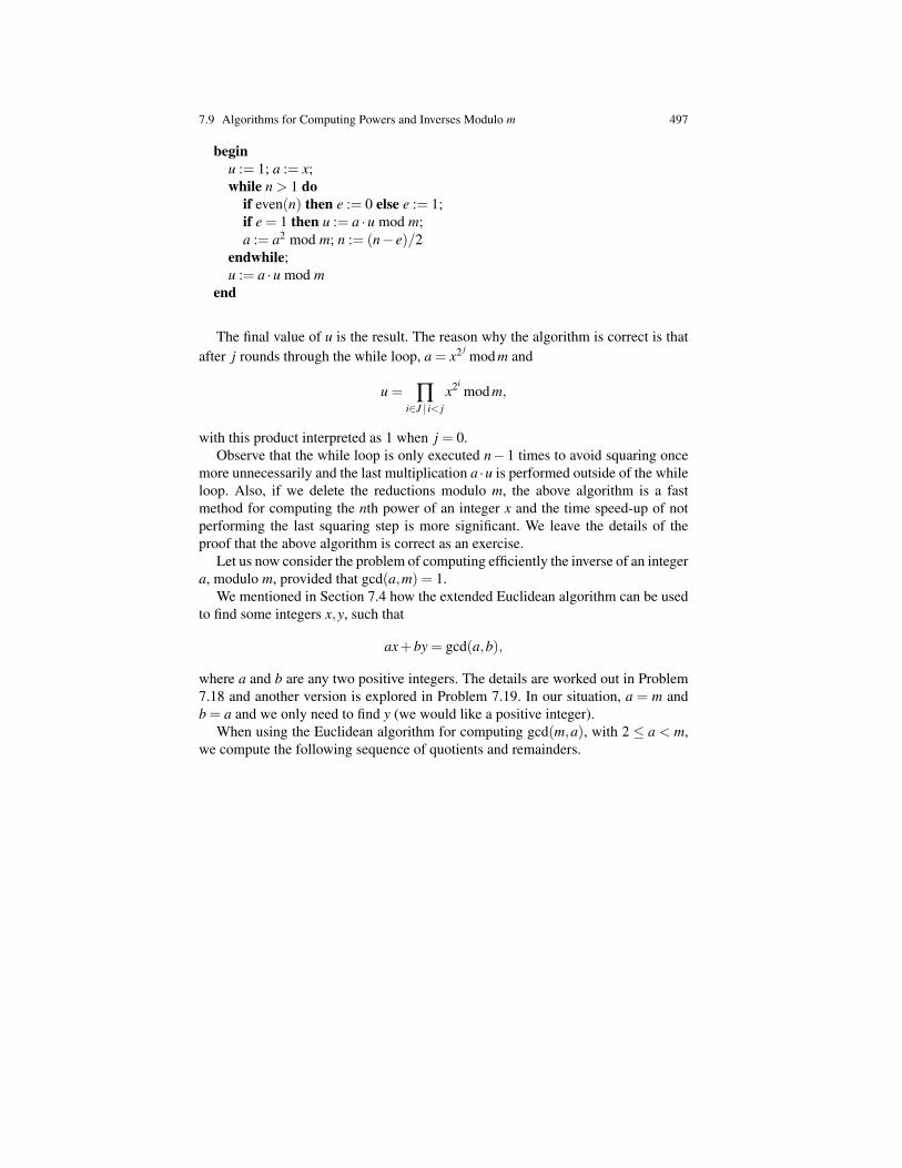
7.9 Algorithms for Computing Powers and Inverses Modulo m 497
beginu := 1; a := x;while n > 1 do
if even(n) then e := 0 else e := 1;if e = 1 then u := a ·u mod m;a := a2 mod m; n := (n− e)/2
endwhile;u := a ·u mod m
end
The final value of u is the result. The reason why the algorithm is correct is thatafter j rounds through the while loop, a = x2 j
mod m and
u = ∏i∈J | i< j
x2imod m,
with this product interpreted as 1 when j = 0.Observe that the while loop is only executed n−1 times to avoid squaring once
more unnecessarily and the last multiplication a ·u is performed outside of the whileloop. Also, if we delete the reductions modulo m, the above algorithm is a fastmethod for computing the nth power of an integer x and the time speed-up of notperforming the last squaring step is more significant. We leave the details of theproof that the above algorithm is correct as an exercise.
Let us now consider the problem of computing efficiently the inverse of an integera, modulo m, provided that gcd(a,m) = 1.
We mentioned in Section 7.4 how the extended Euclidean algorithm can be usedto find some integers x,y, such that
ax+by = gcd(a,b),
where a and b are any two positive integers. The details are worked out in Problem7.18 and another version is explored in Problem 7.19. In our situation, a = m andb = a and we only need to find y (we would like a positive integer).
When using the Euclidean algorithm for computing gcd(m,a), with 2 ≤ a < m,we compute the following sequence of quotients and remainders.

498 7 Partial Orders, GCDs, RSA, Lattices
m = aq1 + r1
a = r1q2 + r2
r1 = r2q3 + r3
...rk−1 = rkqk+1 + rk+1
...rn−3 = rn−2qn−1 + rn−1
rn−2 = rn−1qn +0,
with n≥ 3, 0< r1 < b, qk ≥ 1, for k = 1, . . . ,n, and 0< rk+1 < rk, for k = 1, . . . ,n−2.Observe that rn = 0. If n = 2, we have just two divisions,
m = aq1 + r1
a = r1q2 +0,
with 0 < r1 < b, q1,q2 ≥ 1, and r2 = 0. Thus, it is convenient to set r−1 = m andr0 = a.
In Problem 7.18, it is shown that if we set
x−1 = 1y−1 = 0
x0 = 0y0 = 1
xi+1 = xi−1− xiqi+1
yi+1 = yi−1− yiqi+1,
for i = 0, . . . ,n−2, then
mxn−1 +ayn−1 = gcd(m,a) = rn−1,
and so, if gcd(m,a) = 1, then rn−1 = 1 and we have
ayn−1 ≡ 1 (mod m).
Now, yn−1 may be greater than m or negative but we already know how to deal withthat from the discussion just before Theorem 7.10. This suggests reducing modulom during the recurrence and we are led to the following recurrence.
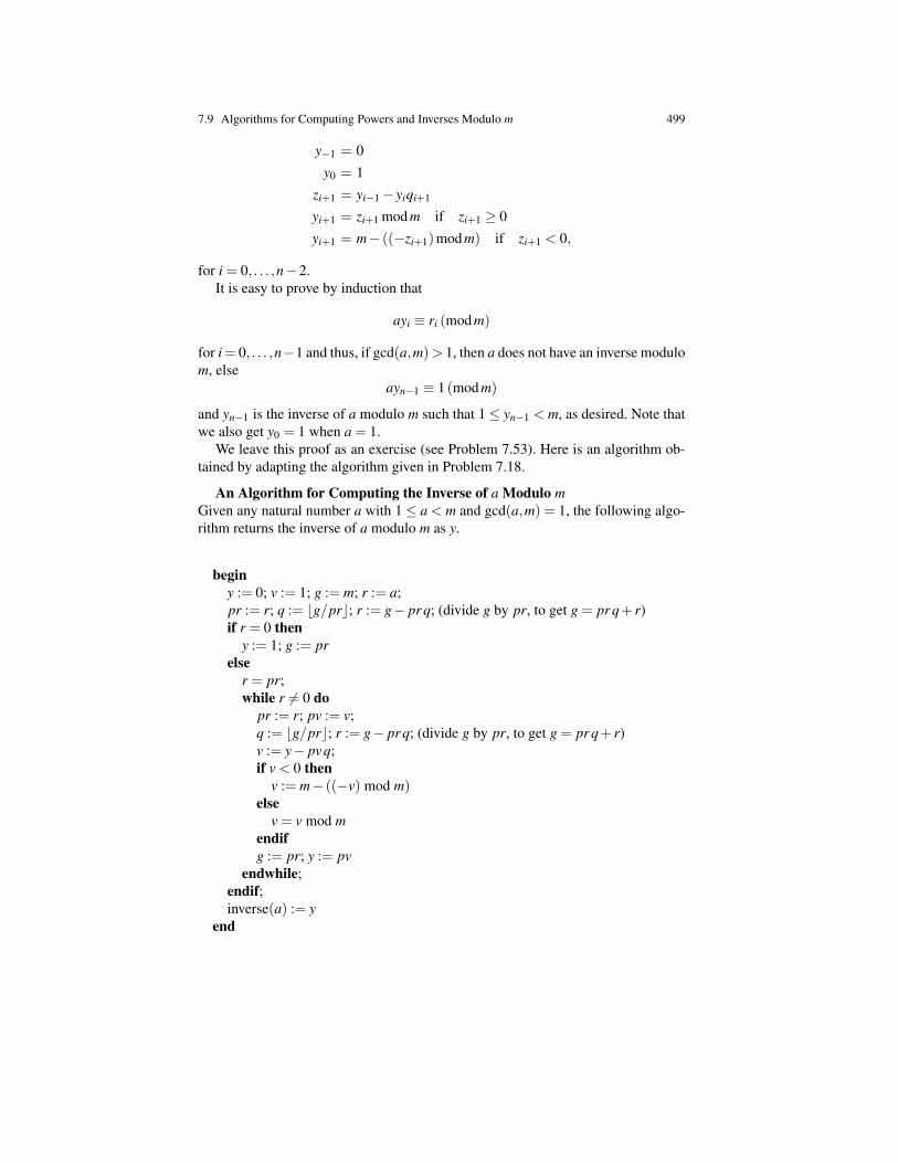
7.9 Algorithms for Computing Powers and Inverses Modulo m 499
y−1 = 0y0 = 1
zi+1 = yi−1− yiqi+1
yi+1 = zi+1 mod m if zi+1 ≥ 0yi+1 = m− ((−zi+1)mod m) if zi+1 < 0,
for i = 0, . . . ,n−2.It is easy to prove by induction that
ayi ≡ ri (mod m)
for i= 0, . . . ,n−1 and thus, if gcd(a,m)> 1, then a does not have an inverse modulom, else
ayn−1 ≡ 1 (mod m)
and yn−1 is the inverse of a modulo m such that 1≤ yn−1 < m, as desired. Note thatwe also get y0 = 1 when a = 1.
We leave this proof as an exercise (see Problem 7.53). Here is an algorithm ob-tained by adapting the algorithm given in Problem 7.18.
An Algorithm for Computing the Inverse of a Modulo mGiven any natural number a with 1≤ a < m and gcd(a,m) = 1, the following algo-rithm returns the inverse of a modulo m as y.
beginy := 0; v := 1; g := m; r := a;pr := r; q := bg/prc; r := g− pr q; (divide g by pr, to get g = pr q+ r)if r = 0 then
y := 1; g := prelse
r = pr;while r 6= 0 do
pr := r; pv := v;q := bg/prc; r := g− pr q; (divide g by pr, to get g = pr q+ r)v := y− pvq;if v < 0 then
v := m− ((−v) mod m)else
v = v mod mendifg := pr; y := pv
endwhile;endif;inverse(a) := y
end

500 7 Partial Orders, GCDs, RSA, Lattices
For example, we used the above algorithm to find that dA = 145,604,785 is theinverse of eA = 79921 modulo (pA−1)(qA−1) = 163,251,312.
The remaining issues are how to choose large random prime numbers p,q, andhow to find a random number e, which is relatively prime to (p−1)(q−1). For this,we rely on a deep result of number theory known as the prime number theorem.
7.10 Finding Large Primes; Signatures; Safety of RSA
Roughly speaking, the prime number theorem ensures that the density of primes ishigh enough to guarantee that there are many primes with a large specified numberof digits. The relevant function is the prime counting function π(n).
Definition 7.10. The prime counting function π is the function defined so that
π(n) = number of prime numbers p, such that p≤ n,
for every natural number n ∈ N.
Obviously, π(0) = π(1) = 0. We have π(10) = 4 because the primes no greaterthan 10 are 2,3,5,7 and π(20) = 8 because the primes no greater than 20 are2,3,5,7,11,13, 17,19. The growth of the function π was studied by Legendre,Gauss,Chebyshev, and Riemann between 1808 and 1859. By then, it was conjec-tured that
π(n)∼ nln(n)
,
for n large, which means that
limn7→∞
π(n)/
nln(n)
= 1.
However, a rigorous proof was not found until 1896. Indeed, in 1896, Jacques
Fig. 7.18 Pafnuty Lvovich Chebyshev, 1821–1894 (left), Jacques Salomon Hadamard, 1865–1963(middle), and Charles Jean de la Vallee Poussin, 1866–1962 (right)
7.10 Finding Large Primes; Signatures; Safety of RSA 501
Hadamard and Charles de la Vallee-Poussin independendly gave a proof of this“most wanted theorem,” using methods from complex analysis. These proofs are dif-ficult and although more elementary proofs were given later, in particular by Erdosand Selberg (1949), those proofs are still quite hard. Thus, we content ourselveswith a statement of the theorem.
Fig. 7.19 Paul Erdos, 1913–1996 (left), Atle Selberg, 1917–2007 (right)
Theorem 7.15. (Prime Number Theorem) For n large, the number of primes π(n)no larger than n is approximately equal to n/ ln(n), which means that
limn7→∞
π(n)/
nln(n)
= 1.
For a rather detailed account of the history of the prime number theorem (forshort, PNT), we refer the reader to Ribenboim [13] (Chapter 4).
As an illustration of the use of the PNT, we can estimate the number of primeswith 200 decimal digits. Indeed this is the difference of the number of primes up to10200 minus the number of primes up to 10199, which is approximately
10200
200ln10− 10199
199ln10≈ 1.95 ·10197.
Thus, we see that there is a huge number of primes with 200 decimal digits. Thenumber of natural numbers with 200 digits is 10200 − 10199 = 9 · 10199, thus theproportion of 200-digit numbers that are prime is
1.95 ·10197
9 ·10199 ≈ 1460
.
Consequently, among the natural numbers with 200 digits, roughly one in every 460is a prime.
Beware that the above argument is not entirely rigorous because the primenumber theorem only yields an approximation of π(n) but sharper estimates
can be used to say how large n should be to guarantee a prescribed error on theprobability, say 1%.
502 7 Partial Orders, GCDs, RSA, Lattices
The implication of the above fact is that if we wish to find a random prime with200 digits, we pick at random some natural number with 200 digits and test whetherit is prime. If this number is not prime, then we discard it and try again, and so on.On the average, after 460 trials, a prime should pop up,
This leads us the question: How do we test for primality?Primality testing has also been studied for a long time. Remarkably, Fermat’s
little theorem yields a test for nonprimality. Indeed, if p > 1 fails to divide ap−1−1for some natural number a, where 2 ≤ a ≤ p− 1, then p cannot be a prime. Thesimplest a to try is a= 2. From a practical point of view, we can compute ap−1 mod pusing the method of repeated squaring and check whether the remainder is 1.
But what if p fails the Fermat test? Unfortunately, there are natural numbers p,such that p divides 2p−1−1 and yet, p is composite. For example p = 341 = 11 ·31is such a number.
Actually, 2340 being quite big, how do we check that 2340−1 is divisible by 341?We just have to show that 2340 − 1 is divisible by 11 and by 31. We can use
Fermat’s little theorem. Because 11 is prime, we know that 11 divides 210−1. But,
2340−1 = (210)34−1 = (210−1)((210)33 +(210)32 + · · ·+1),
so 2340−1 is also divisible by 11.As to divisibility by 31, observe that 31 = 25−1, and
2340−1 = (25)68−1 = (25−1)((25)67 +(25)66 + · · ·+1),
so 2340−1 is also divisible by 31.A number p that is not a prime but behaves like a prime in the sense that p
divides 2p−1− 1, is called a pseudo-prime. Unfortunately, the Fermat test gives a“false positive” for pseudo-primes.
Rather than simply testing whether 2p−1− 1 is divisible by p, we can also trywhether 3p−1−1 is divisible by p and whether 5p−1−1 is divisible by p, and so on.
Unfortunately, there are composite natural numbers p, such that p divides ap−1−1, for all positive natural numbers a with gcd(a, p) = 1. Such numbers are known asCarmichael numbers. The smallest Carmichael number is p = 561 = 3 ·11 ·17. Thereader should try proving that, in fact, a560−1 is divisible by 561 for every positivenatural number a, such that gcd(a,561) = 1, using the technique that we used toprove that 341 divides 2340−1.
It turns out that there are infinitely many Carmichael numbers. Again, for a thor-ough introduction to primality testing, pseudo-primes, Carmichael numbers, andmore, we highly recommend Ribenboim [13] (Chapter 2). An excellent (but moreterse) account is also given in Koblitz [9] (Chapter V).
Still, what do we do about the problem of false positives? The key is to switch toprobabilistic methods. Indeed, if we can design a method that is guaranteed to give afalse positive with probablity less than 0.5, then we can repeat this test for randomlychosen as and reduce the probability of false positive considerably. For example,if we repeat the experiment 100 times, the probability of false positive is less than2−100 < 10−30. This is probably less than the probability of hardware failure.
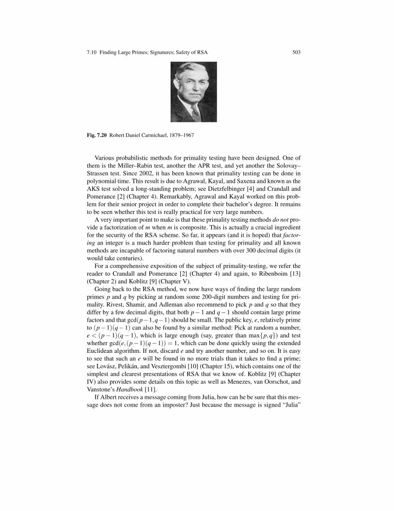
7.10 Finding Large Primes; Signatures; Safety of RSA 503
Fig. 7.20 Robert Daniel Carmichael, 1879–1967
Various probabilistic methods for primality testing have been designed. One ofthem is the Miller–Rabin test, another the APR test, and yet another the Solovay–Strassen test. Since 2002, it has been known that primality testing can be done inpolynomial time. This result is due to Agrawal, Kayal, and Saxena and known as theAKS test solved a long-standing problem; see Dietzfelbinger [4] and Crandall andPomerance [2] (Chapter 4). Remarkably, Agrawal and Kayal worked on this prob-lem for their senior project in order to complete their bachelor’s degree. It remainsto be seen whether this test is really practical for very large numbers.
A very important point to make is that these primality testing methods do not pro-vide a factorization of m when m is composite. This is actually a crucial ingredientfor the security of the RSA scheme. So far, it appears (and it is hoped) that factor-ing an integer is a much harder problem than testing for primality and all knownmethods are incapable of factoring natural numbers with over 300 decimal digits (itwould take centuries).
For a comprehensive exposition of the subject of primality-testing, we refer thereader to Crandall and Pomerance [2] (Chapter 4) and again, to Ribenboim [13](Chapter 2) and Koblitz [9] (Chapter V).
Going back to the RSA method, we now have ways of finding the large randomprimes p and q by picking at random some 200-digit numbers and testing for pri-mality. Rivest, Shamir, and Adleman also recommend to pick p and q so that theydiffer by a few decimal digits, that both p−1 and q−1 should contain large primefactors and that gcd(p−1,q−1) should be small. The public key, e, relatively primeto (p−1)(q−1) can also be found by a similar method: Pick at random a number,e < (p− 1)(q− 1), which is large enough (say, greater than maxp,q) and testwhether gcd(e,(p−1)(q−1)) = 1, which can be done quickly using the extendedEuclidean algorithm. If not, discard e and try another number, and so on. It is easyto see that such an e will be found in no more trials than it takes to find a prime;see Lovasz, Pelikan, and Vesztergombi [10] (Chapter 15), which contains one of thesimplest and clearest presentations of RSA that we know of. Koblitz [9] (ChapterIV) also provides some details on this topic as well as Menezes, van Oorschot, andVanstone’s Handbook [11].
If Albert receives a message coming from Julia, how can he be sure that this mes-sage does not come from an imposter? Just because the message is signed “Julia”

504 7 Partial Orders, GCDs, RSA, Lattices
does not mean that it comes from Julia; it could have been sent by someone elsepretending to be Julia, inasmuch as all that is needed to send a message to Albertis Albert’s public key, which is known to everybody. This leads us to the issue ofsignatures.
There are various schemes for adding a signature to an encrypted message toensure that the sender of a message is really who he or she claims to be (with a highdegree of confidence). The trick is to make use of the the sender’s keys. We proposetwo scenarios.
1. The sender, Julia, encrypts the message x to be sent with her own private key,(dJ ,mJ), creating the message DJ(x) = y1. Then, Julia adds her signature, “Ju-lia”, at the end of the message y1, encrypts the message “y1 Julia” using Albert’spublic key, (eA,mA), creating the message y2 = EA(y1 Julia), and finally sendsthe message y2 to Albert.When Albert receives the encrypted message y2 claiming to come from Julia,first he decrypts the message using his private key (dA,mA). He will see an en-crypted message, DA(y2) = y1 Julia, with the legible signature, Julia. He willthen delete the signature from this message and decrypt the message y1 usingJulia’s public key (eJ ,mJ), getting x = EJ(y1). Albert will know whether some-one else faked this message if the result is garbage. Indeed, only Julia could haveencrypted the original message x with her private key, which is only known toher. An eavesdropper who is pretending to be Julia would not know Julia’s pri-vate key and so, would not have encrypted the original message to be sent usingJulia’s secret key.
2. The sender, Julia, first adds her signature, “Julia”, to the message x to be sentand then, she encrypts the message “x Julia” with Albert’s public key (eA,mA),creating the message y1 = EA(x Julia). Julia also encrypts the original messagex using her private key (dJ ,mJ) creating the message y2 = DJ(x), and finallyshe sends the pair of messages (y1,y2).When Albert receives a pair of messages (y1,y2), claiming to have been sent byJulia, first Albert decrypts y1 using his private key (dA,mA), getting the messageDA(y1) = x Julia. Albert finds the signature, Julia, and then decrypts y2 usingJulia’s public key (eJ ,mJ), getting the message x′=EJ(y2). If x= x′, then Alberthas serious assurance that the sender is indeed Julia and not an imposter.
The last topic that we would like to discuss is the security of the RSA scheme.This is a difficult issue and many researchers have worked on it. As we remarkedearlier, the security of RSA hinges on the fact that factoring is hard. It has beenshown that if one has a method for breaking the RSA scheme (namely, to find thesecret key d), then there is a probabilistic method for finding the factors p and q,of m = pq (see Koblitz [9], Chapter IV, Section 2, or Menezes, van Oorschot, andVanstone [11], Section 8.2.2). If p and q are chosen to be large enough, factoringm = pq will be practically impossible and so it is unlikely that RSA can be cracked.However, there may be other attacks and, at present, there is no proof that RSA isfully secure.
7.11 Distributive Lattices, Boolean Algebras, Heyting Algebras 505
Observe that because m = pq is known to everybody, if somehow one can learnN = (p− 1)(q− 1), then p and q can be recovered. Indeed N = (p− 1)(q− 1) =pq− (p+q)+1 = m− (p+q)+1 and so,
pq = m
p+q = m−N +1,
and p and q are the roots of the quadratic equation
X2− (m−N +1)X +m = 0.
Thus, a line of attack is to try to find the value of (p− 1)(q− 1). For more on thesecurity of RSA, see Menezes, van Oorschot, and Vanstone’s Handbook [11].
7.11 Distributive Lattices, Boolean Algebras, Heyting Algebras
If we go back to one of our favorite examples of a lattice, namely, the power set2X of some set X , we observe that it is more than a lattice. For example, if we lookat Figure 7.6, we can check that the two identities D1 and D2 stated in the nextdefinition hold.
Definition 7.11. We say that a lattice X is a distributive lattice if (D1) and (D2)hold:
D1 a∧ (b∨ c) = (a∧b)∨ (a∧ c)
D2 a∨ (b∧ c) = (a∨b)∧ (a∨ c).
Remark: Not every lattice is distributive but many lattices of interest are distribu-tive.
It is a bit surprising that in a lattice (D1) and (D2) are actually equivalent, as wenow show. Suppose (D1) holds, then
(a∨b)∧ (a∨ c) = ((a∨b)∧a)∨ ((a∨b)∧ c) (D1)= a∨ ((a∨b)∧ c) (L4)= a∨ ((c∧ (a∨b)) (L1)= a∨ ((c∧a)∨ (c∧b)) (D1)= a∨ ((a∧ c)∨ (b∧ c)) (L1)= (a∨ (a∧ c))∨ (b∧ c) (L2)= ((a∧ c)∨a)∨ (b∧ c) (L1)= a∨ (b∧ c) (L4)
which is (D2). Dually, (D2) implies (D1).
506 7 Partial Orders, GCDs, RSA, Lattices
The reader should prove that every totally ordered poset is a distributive lattice.The lattice N+ = N−0 under the divisibility ordering also turns out to be a dis-tributive lattice.
Another useful fact about distributivity is that in any lattice
a∧ (b∨ c)≥ (a∧b)∨ (a∧ c).
This is because in any lattice, a∧ (b∨ c)≥ a∧b and a∧ (b∨ c)≥ a∧ c. Therefore,in order to establish distributivity in a lattice it suffices to show that
a∧ (b∨ c)≤ (a∧b)∨ (a∧ c).
Another important property of distributive lattices is the following.
Proposition 7.21. In a distributive lattice X, if z∧ x = z∧ y and z∨ x = z∨ y, thenx = y (for all x,y,z ∈ X).
Proof . We have
x = (x∨ z)∧ x (L4)= x∧ (z∨ x) (L1)= x∧ (z∨ y)
= (x∧ z)∨ (x∧ y) (D1)
= (z∧ x)∨ (x∧ y) (L1)= (z∧ y)∨ (x∧ y)
= (y∧ z)∨ (y∧ x) (L1)= y∧ (z∨ x) (D1)= y∧ (z∨ y)
= (y∨ z)∧ y (L1)= y; (L4)
that is, x = y, as claimed. ut
The power set lattice has yet some additional properties having to do with com-plementation. First, the power lattice 2X has a least element 0 = /0 and a greatestelement, 1 = X . If a lattice X has a least element 0 and a greatest element 1, thefollowing properties are clear: For all a ∈ X , we have
a∧0 = 0 a∨0 = a
a∧1 = a a∨1 = 1.
More important, for any subset A ⊆ X we have the complement A of A in X ,which satisfies the identities:
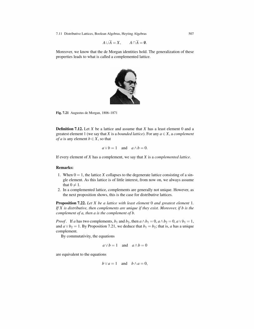
7.11 Distributive Lattices, Boolean Algebras, Heyting Algebras 507
A∪A = X , A∩A = /0.
Moreover, we know that the de Morgan identities hold. The generalization of theseproperties leads to what is called a complemented lattice.
Fig. 7.21 Augustus de Morgan, 1806–1871
Definition 7.12. Let X be a lattice and assume that X has a least element 0 and agreatest element 1 (we say that X is a bounded lattice). For any a∈ X , a complementof a is any element b ∈ X , so that
a∨b = 1 and a∧b = 0.
If every element of X has a complement, we say that X is a complemented lattice.
Remarks:
1. When 0 = 1, the lattice X collapses to the degenerate lattice consisting of a sin-gle element. As this lattice is of little interest, from now on, we always assumethat 0 6= 1.
2. In a complemented lattice, complements are generally not unique. However, asthe next proposition shows, this is the case for distributive lattices.
Proposition 7.22. Let X be a lattice with least element 0 and greatest element 1.If X is distributive, then complements are unique if they exist. Moreover, if b is thecomplement of a, then a is the complement of b.
Proof . If a has two complements, b1 and b2, then a∧b1 = 0, a∧b2 = 0, a∨b1 = 1,and a∨b2 = 1. By Proposition 7.21, we deduce that b1 = b2; that is, a has a uniquecomplement.
By commutativity, the equations
a∨b = 1 and a∧b = 0
are equivalent to the equations
b∨a = 1 and b∧a = 0,
508 7 Partial Orders, GCDs, RSA, Lattices
which shows that a is indeed a complement of b. By uniqueness, a is the complementof b. ut
In view of Proposition 7.22, if X is a complemented distributive lattice, we denotethe complement of any element, a ∈ X , by a. We have the identities
a∨a = 1a∧a = 0
a = a.
We also have the following proposition about the de Morgan laws.
Proposition 7.23. Let X be a lattice with least element 0 and greatest element 1. IfX is distributive and complemented, then the de Morgan laws hold:
a∨b = a∧b
a∧b = a∨b.
Proof . We prove thata∨b = a∧b,
leaving the dual identity as an easy exercise. Using the uniqueness of complements,it is enough to check that a∧ b works, that is, satisfies the conditions of Definition7.12. For the first condition, we have
(a∨b)∨ (a∧b) = ((a∨b)∨a)∧ ((a∨b)∨b)
= (a∨ (b∨a))∧ (a∨ (b∨b))
= (a∨ (a∨b))∧ (a∨1)= ((a∨a)∨b)∧1= (1∨b)∧1= 1∧1 = 1.
For the second condition, we have
(a∨b)∧ (a∧b) = (a∧ (a∧b))∨ (b∧ (a∧b))
= ((a∧a)∧b)∨ (b∧ (b∧a))
= (0∧b)∨ ((b∧b)∧a)
= 0∨ (0∧a)
= 0∨0 = 0.
ut
All this leads to the definition of a Boolean lattice.
Definition 7.13. A Boolean lattice is a lattice with a least element 0, a greatest ele-ment 1, and which is distributive and complemented.
7.11 Distributive Lattices, Boolean Algebras, Heyting Algebras 509
Of course, every power set is a Boolean lattice, but there are Boolean latticesthat are not power sets. Putting together what we have done, we see that a Booleanlattice is a set X with two special elements, 0, 1, and three operations ∧, ∨, anda 7→ a satisfying the axioms stated in the following.
Proposition 7.24. If X is a Boolean lattice, then the following equations hold for alla,b,c ∈ X.
L1 a∨b = b∨a, a∧b = b∧a
L2 (a∨b)∨ c = a∨ (b∨ c), (a∧b)∧ c = a∧ (b∧ c)
L3 a∨a = a, a∧a = a
L4 (a∨b)∧a = a, (a∧b)∨a = a
D1-D2 a∧ (b∨ c) = (a∧b)∨ (a∧ c), a∨ (b∧ c) = (a∨b)∧ (a∨ c)
LE a∨0 = a, a∧0 = 0GE a∨1 = 1, a∧1 = a
C a∨a = 1, a∧a = 0I a = a
dM a∨b = a∧b, a∧b = a∨b.
Conversely, if X is a set together with two special elements 0, 1, and three operations∧, ∨, and a 7→ a satisfying the axioms above, then it is a Boolean lattice under theordering given by a≤ b iff a∨b = b.
In view of Proposition 7.24, we make the following definition.
Definition 7.14. A set X together with two special elements 0, 1 and three opera-tions ∧, ∨, and a 7→ a satisfying the axioms of Proposition 7.24 is called a Booleanalgebra.
Proposition 7.24 shows that the notions of a Boolean lattice and of a Boolean al-gebra are equivalent. The first one is order-theoretic and the second one is algebraic.
Remarks:
1. As the name indicates, Boolean algebras were invented by G. Boole (1854).One of the first comprehensive accounts is due to E. Schroder (1890–1895).
2. The axioms for Boolean algebras given in Proposition 7.24 are not independent.There is a set of independent axioms known as the Huntington axioms (1933).
Let p be any integer with p ≥ 2. Under the division ordering, it turns out thatthe set Div(p) of divisors of p is a distributive lattice. In general not every integerk ∈Div(p) has a complement but when it does k = p/k. It can be shown that Div(p)is a Boolean algebra iff p is not divisible by any square integer (an integer of theform m2, with m > 1).
Classical logic is also a rich source of Boolean algebras. Indeed, it is easy toshow that logical equivalence is an equivalence relation and, as homework prob-lems, you have shown (with great pain) that all the axioms of Proposition 7.24 are
510 7 Partial Orders, GCDs, RSA, Lattices
Fig. 7.22 George Boole, 1815–1864 (left) and Ernst Schroder 1841–1902 (right)
provable equivalences (where ∨ is disjunction and ∧ is conjunction, P = ¬P; i.e.,negation, 0 =⊥ and 1 = >) (see Problems 2.8, 2.18, 2.28). Furthermore, again, ashomework problems (see Problems 2.18–2.20), you have shown that logical equiv-alence is compatible with ∨,∧,¬ in the following sense. If P1 ≡ Q1 and P2 ≡ Q2,then
(P1∨P2) ≡ (Q1∨Q2)
(P1∧P2) ≡ (Q1∧Q2)
¬P1 ≡ ¬Q1.
Consequently, for any set T of propositions we can define the relation ≡T by
P≡T Q iff T ` P≡ Q,
that is, iff P ≡ Q is provable from T (as explained in Section 2.11). Clearly, ≡T isan equivalence relation on propositions and so, we can define the operations ∨,∧,and on the set of equivalence classes BT of propositions as follows.
[P]∨ [Q] = [P∨Q]
[P]∧ [Q] = [P∧Q]
[P] = [¬P].
We also let 0 = [⊥] and 1 = [>]. Then, we get the Boolean algebra BT called theLindenbaum algebra of T .
It also turns out that Boolean algebras are just what’s needed to give truth-valuesemantics to classical logic. Let B be any Boolean algebra. A truth assignment is anyfunction v from the set PS = P1,P2, . . . of propositional symbols to B. Then, wecan recursively evaluate the truth value PB[v] in B of any proposition P with respectto the truth assignment v as follows.

7.11 Distributive Lattices, Boolean Algebras, Heyting Algebras 511
(Pi)B[v] = v(P)
⊥B [v] = 0>B[v] = 1
(P∨Q)B[v] = PB[v]∨PB[v]
(P∧Q)B[v] = PB[v]∧PB[v]
(¬P)B[v] = P[v]B.
In the equations above, on the right-hand side, ∨ and ∧ are the lattice operations ofthe Boolean algebra B. We say that a proposition P is valid in the Boolean algebraB (or B-valid) if PB[v] = 1 for all truth assignments v. We say that P is (classically)valid if P is B-valid in all Boolean algebras B. It can be shown that every provableproposition is valid. This property is called soundness. Conversely, if P is valid, thenit is provable. This second property is called completeness. Actually completenessholds in a much stronger sense: If a proposition is valid in the two-element Booleanalgebra 0,1, then it is provable.
One might wonder if there are certain kinds of algebras similar to Boolean alge-bras well suited for intuitionistic logic. The answer is yes: such algebras are calledHeyting algebras.
Fig. 7.23 Arend Heyting, 1898–1980
In our study of intuitionistic logic, we learned that negation is not a primaryconnective but instead it is defined in terms of implication by ¬P = P⇒⊥. Thissuggests adding to the two lattice operations ∨ and ∧ a new operation→, that willbehave like⇒. The trick is, what kind of axioms should we require on→ to “cap-ture” the properties of intuitionistic logic? Now, if X is a lattice with 0 and 1, givenany two elements a,b ∈ X , experience shows that a→ b should be the largest ele-ment c, such that c∧a≤ b. This leads to
Definition 7.15. A lattice X with 0 and 1 is a Heyting lattice iff it has a third binaryoperation→ such that
c∧a≤ b iff c≤ (a→ b)
for all a,b,c ∈ X . We define the negation (or pseudo-complement) of a asa = (a→ 0).
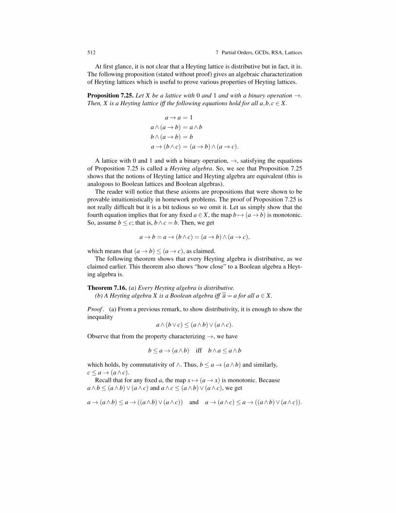
512 7 Partial Orders, GCDs, RSA, Lattices
At first glance, it is not clear that a Heyting lattice is distributive but in fact, it is.The following proposition (stated without proof) gives an algebraic characterizationof Heyting lattices which is useful to prove various properties of Heyting lattices.
Proposition 7.25. Let X be a lattice with 0 and 1 and with a binary operation →.Then, X is a Heyting lattice iff the following equations hold for all a,b,c ∈ X.
a→ a = 1a∧ (a→ b) = a∧b
b∧ (a→ b) = b
a→ (b∧ c) = (a→ b)∧ (a→ c).
A lattice with 0 and 1 and with a binary operation, →, satisfying the equationsof Proposition 7.25 is called a Heyting algebra. So, we see that Proposition 7.25shows that the notions of Heyting lattice and Heyting algebra are equivalent (this isanalogous to Boolean lattices and Boolean algebras).
The reader will notice that these axioms are propositions that were shown to beprovable intuitionistically in homework problems. The proof of Proposition 7.25 isnot really difficult but it is a bit tedious so we omit it. Let us simply show that thefourth equation implies that for any fixed a∈ X , the map b 7→ (a→ b) is monotonic.So, assume b≤ c; that is, b∧ c = b. Then, we get
a→ b = a→ (b∧ c) = (a→ b)∧ (a→ c),
which means that (a→ b)≤ (a→ c), as claimed.The following theorem shows that every Heyting algebra is distributive, as we
claimed earlier. This theorem also shows “how close” to a Boolean algebra a Heyt-ing algebra is.
Theorem 7.16. (a) Every Heyting algebra is distributive.(b) A Heyting algebra X is a Boolean algebra iff a = a for all a ∈ X.
Proof . (a) From a previous remark, to show distributivity, it is enough to show theinequality
a∧ (b∨ c)≤ (a∧b)∨ (a∧ c).
Observe that from the property characterizing→, we have
b≤ a→ (a∧b) iff b∧a≤ a∧b
which holds, by commutativity of ∧. Thus, b≤ a→ (a∧b) and similarly,c≤ a→ (a∧ c).
Recall that for any fixed a, the map x 7→ (a→ x) is monotonic. Becausea∧b≤ (a∧b)∨ (a∧ c) and a∧ c≤ (a∧b)∨ (a∧ c), we get
a→ (a∧b)≤ a→ ((a∧b)∨ (a∧c)) and a→ (a∧c)≤ a→ ((a∧b)∨ (a∧c)).
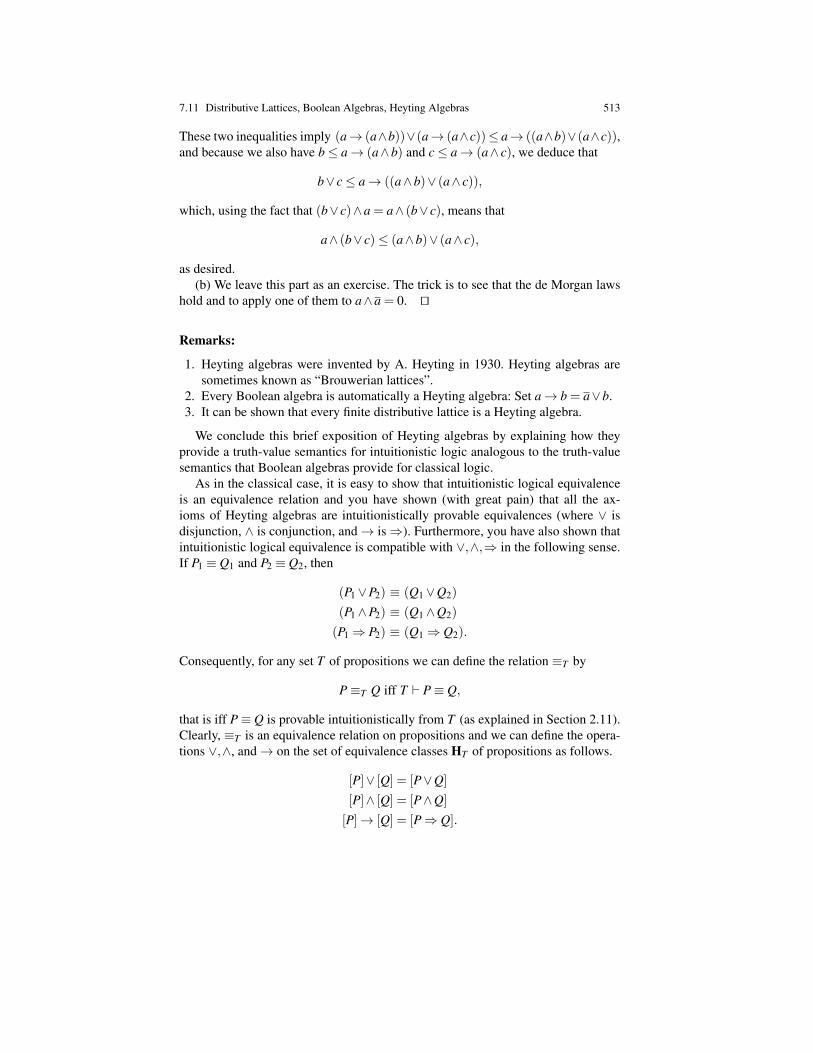
7.11 Distributive Lattices, Boolean Algebras, Heyting Algebras 513
These two inequalities imply (a→ (a∧b))∨(a→ (a∧c))≤ a→ ((a∧b)∨(a∧c)),and because we also have b≤ a→ (a∧b) and c≤ a→ (a∧ c), we deduce that
b∨ c≤ a→ ((a∧b)∨ (a∧ c)),
which, using the fact that (b∨ c)∧a = a∧ (b∨ c), means that
a∧ (b∨ c)≤ (a∧b)∨ (a∧ c),
as desired.(b) We leave this part as an exercise. The trick is to see that the de Morgan laws
hold and to apply one of them to a∧a = 0. ut
Remarks:
1. Heyting algebras were invented by A. Heyting in 1930. Heyting algebras aresometimes known as “Brouwerian lattices”.
2. Every Boolean algebra is automatically a Heyting algebra: Set a→ b = a∨b.3. It can be shown that every finite distributive lattice is a Heyting algebra.
We conclude this brief exposition of Heyting algebras by explaining how theyprovide a truth-value semantics for intuitionistic logic analogous to the truth-valuesemantics that Boolean algebras provide for classical logic.
As in the classical case, it is easy to show that intuitionistic logical equivalenceis an equivalence relation and you have shown (with great pain) that all the ax-ioms of Heyting algebras are intuitionistically provable equivalences (where ∨ isdisjunction, ∧ is conjunction, and→ is⇒). Furthermore, you have also shown thatintuitionistic logical equivalence is compatible with ∨,∧,⇒ in the following sense.If P1 ≡ Q1 and P2 ≡ Q2, then
(P1∨P2) ≡ (Q1∨Q2)
(P1∧P2) ≡ (Q1∧Q2)
(P1⇒ P2) ≡ (Q1⇒ Q2).
Consequently, for any set T of propositions we can define the relation ≡T by
P≡T Q iff T ` P≡ Q,
that is iff P≡ Q is provable intuitionistically from T (as explained in Section 2.11).Clearly, ≡T is an equivalence relation on propositions and we can define the opera-tions ∨,∧, and→ on the set of equivalence classes HT of propositions as follows.
[P]∨ [Q] = [P∨Q]
[P]∧ [Q] = [P∧Q]
[P]→ [Q] = [P⇒ Q].
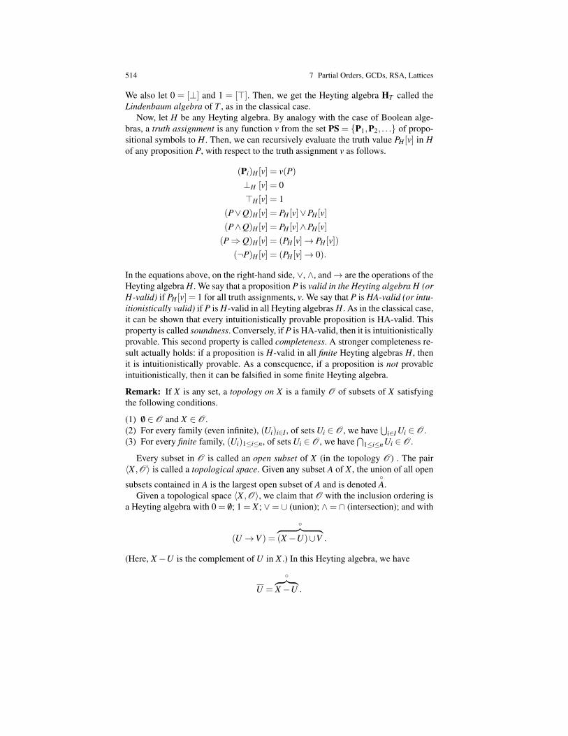
514 7 Partial Orders, GCDs, RSA, Lattices
We also let 0 = [⊥] and 1 = [>]. Then, we get the Heyting algebra HT called theLindenbaum algebra of T , as in the classical case.
Now, let H be any Heyting algebra. By analogy with the case of Boolean alge-bras, a truth assignment is any function v from the set PS = P1,P2, . . . of propo-sitional symbols to H. Then, we can recursively evaluate the truth value PH [v] in Hof any proposition P, with respect to the truth assignment v as follows.
(Pi)H [v] = v(P)
⊥H [v] = 0>H [v] = 1
(P∨Q)H [v] = PH [v]∨PH [v]
(P∧Q)H [v] = PH [v]∧PH [v]
(P⇒ Q)H [v] = (PH [v]→ PH [v])
(¬P)H [v] = (PH [v]→ 0).
In the equations above, on the right-hand side, ∨, ∧, and→ are the operations of theHeyting algebra H. We say that a proposition P is valid in the Heyting algebra H (orH-valid) if PH [v] = 1 for all truth assignments, v. We say that P is HA-valid (or intu-itionistically valid) if P is H-valid in all Heyting algebras H. As in the classical case,it can be shown that every intuitionistically provable proposition is HA-valid. Thisproperty is called soundness. Conversely, if P is HA-valid, then it is intuitionisticallyprovable. This second property is called completeness. A stronger completeness re-sult actually holds: if a proposition is H-valid in all finite Heyting algebras H, thenit is intuitionistically provable. As a consequence, if a proposition is not provableintuitionistically, then it can be falsified in some finite Heyting algebra.
Remark: If X is any set, a topology on X is a family O of subsets of X satisfyingthe following conditions.
(1) /0 ∈ O and X ∈ O .(2) For every family (even infinite), (Ui)i∈I , of sets Ui ∈ O , we have
⋃i∈I Ui ∈ O .
(3) For every finite family, (Ui)1≤i≤n, of sets Ui ∈ O , we have⋂
1≤i≤n Ui ∈ O .
Every subset in O is called an open subset of X (in the topology O) . The pair〈X ,O〉 is called a topological space. Given any subset A of X , the union of all open
subsets contained in A is the largest open subset of A and is denotedA.
Given a topological space 〈X ,O〉, we claim that O with the inclusion ordering isa Heyting algebra with 0 = /0; 1 = X ; ∨= ∪ (union); ∧= ∩ (intersection); and with
(U →V ) =
︷ ︸︸ ︷(X−U)∪V .
(Here, X−U is the complement of U in X .) In this Heyting algebra, we have
U =
︷ ︸︸ ︷X−U .

7.12 Summary 515
Because X −U is usually not open, we generally have U 6= U . Therefore, we seethat topology yields another supply of Heyting algebras.
7.12 Summary
In this chapter, we introduce partial orders and we study some of their main prop-erties. The ability to use induction to prove properties of the elements of a par-tially ordered set is related to a property known as well-foundedness. We investigatequite thoroughly induction principles valid for well-ordered sets and, more gener-ally, well-founded sets. As an application, we prove the unique prime factorizationtheorem for the integers. Section 7.6 on Fibonacci and Lucas numbers and the useof Lucas numbers to test a Mersenne number for primality should be viewed as alovely illustration of complete induction and as an incentive for the reader to take adeeper look into the fascinating and mysterious world of prime numbers and moregenerally, number theory. Section 7.7 on public key cryptography and the RSA sys-tem is a wonderful application of the notions presented in Section 7.4, gcd andversions of Euclid’s algorithm, and another excellent motivation for delving furtherinto number theory. An excellent introduction to the theory of prime numbers with acomputational emphasis is Crandall and Pomerance [2] and a delightful and remark-ably clear introduction to number theory can be found in Silverman [15]. We alsoinvestigate the properties of partially ordered sets where the partial order has someextra properties. For example, we briefly study lattices, complete lattices, Booleanalgebras, and Heyting algebras. Regarding complete lattices, we prove a beautifultheorem due to Tarski (Tarski’s fixed-point theorem) and use it to give a very shortproof of the Schroder–Bernstein theorem (Theorem 3.9).
• We begin with the definition of a partial order.• Next, we define total orders, chains, strict orders, and posets.• We define a minimal element, an immediate predecessor, a maximal element,
and an immediate successor.• We define the Hasse diagram of a poset.• We define a lower bound, and upper bound, a least element, a greatest element,
a greatest lower bound, and a least upper bound.• We define a meet and a join.• We state Zorn’s lemma.• We define monotonic functions.• We define lattices and complete lattices.• We prove some basic properties of lattices and introduce duality.• We define fixed points as well as least and greatest fixed points.• We state and prove Tarski’s fixed-point theorem.• As a consequence of Tarski’s fixed-point theorem we give a short proof of the
Schroder–Bernstein theorem (Theorem 3.9).• We define a well order and show that N is well ordered.
516 7 Partial Orders, GCDs, RSA, Lattices
• We revisit complete induction on N and prove its validity.• We define prime numbers and we apply complete induction to prove that every
natural number n≥ 2 can be factored as a product of primes.• We prove that there are infinitely many primes.• We use the fact that N is well ordered to prove the correctness of Euclidean
division.• We define well-founded orderings.• We characterize well-founded orderings in terms of minimal elements.• We define the principle of complete induction on a well-founded set and prove
its validity.• We define the lexicographic ordering on pairs.• We give the example of Ackermann’s function and prove that it is a total func-
tion.• We define divisibility on Z (the integers).• We define ideals and prime ideals of Z.• We prove that every ideal of Z is a principal ideal.• We prove the Bezout identity.• We define greatest common divisors (gcds) and relatively prime numbers.• We characterize gcds in terms of the Bezout identity.• We describe the Euclidean algorithm for computing the gcd and prove its cor-
rectness.• We prove Euclid’s lemma.• We prove unique prime factorization in N.• We prove Dirichlet’s diophantine approximation theorem, a great application of
the pigeonhole principle• We define the Fibonacci numbers Fn and the Lucas numbers Ln, and investigate
some of their properties, including explicit formulae for Fn and Ln.• We state the Zeckendorf representation of natural numbers in terms of Fibonacci
numbers.• We give various versions of the Cassini identity• We define a generalization of the Fibonacci and the Lucas numbers and state
some of their properties.• We define Mersenne numbers and Mersenne primes.• We state two versions of the Lucas–Lehmer test to check whether a Mersenne
number is a prime.• We introduce some basic notions of cryptography: encryption, decryption, and
keys.• We define modular arithmetic in Z/mZ.• We define the notion of a trapdoor one-way function.• We claim that exponentiation modulo m is a trapdoor one-way function; its in-
verse is the discrete logarithm.• We explain how to set up the RSA scheme; we describe public keys and private
keys.• We describe the procedure to encrypt a message using RSA and the procedure
to decrypt a message using RSA.
7.12 Problems 517
• We prove Fermat’s little theorem.• We prove the correctness of the RSA scheme.• We describe an algorithm for computing xn mod m using repeated squaring and
give an example.• We give an explicit example of an RSA scheme and an explicit example of the
decryption of a message.• We explain how to modify the extended Euclidean algorithm to find the inverse
of an integer a modulo m (assuming gcd(a,m) = 1).• We define the prime counting function, π(n), and state the prime number theo-
rem (or PNT).• We use the PNT to estimate the proportion of primes among positive integers
with 200 decimal digits (1/460).• We discuss briefly primality testing and the Fermat test.• We define pseudo-prime numbers and Carmichael numbers.• We mention probabilistic methods for primality testing.• We stress that factoring integers is a hard problem, whereas primality testing is
much easier and in theory, can be done in polynomial time.• We discuss briefly scenarios for signatures.• We briefly discuss the security of RSA, which hinges on the fact that factoring
is hard.• We define distributive lattices and prove some properties about them.• We define complemented lattices and prove some properties about them.• We define Boolean lattices, state some of their properties, and define Boolean
algebras.• We discuss the Boolean-valued semantics of classical logic.• We define the Lindenbaum algebra of a set of propositions.• We define Heyting lattices and prove some properties about them and define
Heyting algebras.• We show that every Heyting algebra is distributive and characterize when a
Heyting algebra is a Boolean algebra.• We discuss the semantics of intuitionistic logic in terms of Heyting algebras
(HA-validity).• We conclude with the definition of a topological space and show how the open
sets form a Heyting algebra.
Problems
7.1. Give a proof for Proposition 7.1.
7.2. Give a proof for Proposition 7.2.
7.3. Draw the Hasse diagram of all the (positive) divisors of 60, where the partialordering is the division ordering (i.e., a ≤ b iff a divides b). Does every pair ofelements have a meet and a join?

518 7 Partial Orders, GCDs, RSA, Lattices
7.4. Check that the lexicographic ordering on strings is indeed a total order.
7.5. Check that the function ϕ : 2A → 2A used in the proof of Theorem 3.9, is in-deed monotonic. Check that the function h : A→ B constructed during the proof ofTheorem 3.9, is indeed a bijection.
7.6. Give an example of a poset in which complete induction fails.
7.7. Prove that the lexicographic ordering << on pairs is indeed a partial order.
7.8. Prove that the setI= ha+ kb | h,k ∈ Z
used in the proof of Corollary 7.2 is indeed an ideal.
7.9. Prove by complete induction that
un = 3(3n−2n)
is the solution of the recurrence relations:
u0 = 0u1 = 3
un+2 = 5un+1−6un,
for all n≥ 0.
7.10. Consider the recurrence relation
un+2 = 3un+1−2un.
For u0 = 0 and u1 = 1, we obtain the sequence (Un) and for u0 = 2 and u1 = 3, weobtain the sequence (Vn).
(1) Prove that
Un = 2n−1Vn = 2n +1,
for all n≥ 0.(2) Prove that if Un is a prime number, then n must be a prime number.
Hint. Use the fact that
2ab−1 = (2a−1)(1+2a +22a + · · ·+2(b−1)a).
Remark: The numbers of the form 2p−1, where p is prime are known as Mersennenumbers. It is an open problem whether there are infinitely many Mersenne primes.
7.12 Problems 519
(3) Prove that if Vn is a prime number, then n must be a power of 2; that is, n= 2m,for some natural number m.Hint. Use the fact that
a2k+1 +1 = (a+1)(a2k−a2k−1 +a2k−2 + · · ·+a2−a+1).
Remark: The numbers of the form 22m+1 are known as Fermat numbers. It is an
open problem whether there are infinitely many Fermat primes.
7.11. Find the smallest natural number n such that the remainder of the division ofn by k is k−1, for k = 2,3,4, . . . ,10.
7.12. Prove that if z is a real zero of a polynomial equation of the form
zn +an−1zn−1 + · · ·+a1z+a0 = 0,
where a0,a1, . . . ,an−1 are integers and z is not an integer, then z must be irrational.
7.13. Prove that for every integer k ≥ 2 there is some natural number n so that the kconsecutive numbers, n+1, . . . ,n+ k, are all composite (not prime).Hint. Consider sequences starting with (k+1)!+2.
7.14. Let p be any prime number. (1) Prove that for every k, with 1≤ k≤ p−1, theprime p divides
(pk
).
Hint. Observe that
k(
pk
)= p(
p−1k−1
).
(2) Prove that for every natural number a, if p is prime then p divides ap−a.Hint. Use induction on a.
Deduce Fermat’s little theorem: For any prime p and any natural number a, if pdoes not divide a, then p divides ap−1−1.
7.15. If one wants to prove a property P(n) of the natural numbers, rather than usinginduction, it is sometimes more convenient to use the method of proof by smallestcounterexample. This is a method that proceeds by contradiction as follows.
1. If P is false, then we know from Theorem 7.3 that there is a smallest k ∈N suchthat P(k) is false; this k is the smallest counterexample.
2. Next, we prove that k 6= 0. This is usually easy and it is a kind of basis step.3. Because k 6= 0, the number k− 1 is a natural number and P(k− 1) must hold
because k is the smallest counterexample. Then, use this fact and the fact thatP(k) is false to derive a contradiction.
Use the method of proof by smallest counterexample to prove that every naturalnumber is either odd or even.
7.16. Prove that for any two positive natural numbers a and m, if gcd(a,m)> 1, then
am−1 6≡ 1 (mod m).
520 7 Partial Orders, GCDs, RSA, Lattices
7.17. Let a,b be any two positive integers. (1) Prove that if a is even and b odd, then
gcd(a,b) = gcd(a
2,b).
(2) Prove that if both a and b are even, then
gcd(a,b) = 2gcd(
a2,
b2
).
7.18. Let a,b be any two positive integers and assume a ≥ b. When using the Eu-clidean alorithm for computing the gcd, we compute the following sequence of quo-tients and remainders.
a = bq1 + r1
b = r1q2 + r2
r1 = r2q3 + r3
...rk−1 = rkqk+1 + rk+1
...rn−3 = rn−2qn−1 + rn−1
rn−2 = rn−1qn +0,
with n≥ 3, 0< r1 < b, qk ≥ 1, for k = 1, . . . ,n, and 0< rk+1 < rk, for k = 1, . . . ,n−2.Observe that rn = 0.
If n = 1, we have a single division,
a = bq1 +0,
with r1 = 0 and q1 ≥ 1 and if n = 2, we have two divisions,
a = bq1 + r1
b = r1q2 +0
with 0 < r1 < b, q1,q2 ≥ 1 and r2 = 0. Thus, it is convenient to set r−1 = a andr0 = b, so that the first two divisions are also written as
r−1 = r0q1 + r1
r0 = r1q2 + r2.
(1) Prove (using Proposition 7.7) that rn−1 = gcd(a,b).(2) Next, we prove that some integers x,y such that
ax+by = gcd(a,b) = rn−1
7.12 Problems 521
can be found as follows:If n = 1, then a = bq1 and r0 = b, so we set x = 1 and y =−(q1−1).If n≥ 2, we define the sequence (xi,yi) for i = 0, . . . ,n−1, so that
x0 = 0, y0 = 1, x1 = 1, y1 =−q1
and, if n≥ 3, then
xi+1 = xi−1− xiqi+1, yi+1 = yi−1− yiqi+1,
for i = 1, . . . ,n−2.Prove that if n≥ 2, then
axi +byi = ri,
for i = 0, . . . ,n−1 (recall that r0 = b) and thus, that
axn−1 +byn−1 = gcd(a,b) = rn−1.
(3) When n≥ 2, if we set x−1 = 1 and y−1 = 0 in addition to x0 = 0 and y0 = 1,then prove that the recurrence relations
xi+1 = xi−1− xiqi+1, yi+1 = yi−1− yiqi+1,
are valid for i = 0, . . . ,n−2.
Remark: Observe that ri+1 is given by the formula
ri+1 = ri−1− riqi+1.
Thus, the three sequences, (ri), (xi), and (yi) all use the same recurrence relation,
wi+1 = wi−1−wiqi+1,
but they have different initial conditions: The sequence ri starts with r−1 = a,r0 = b,the sequence xi starts with x−1 = 1,x0 = 0, and the sequence yi starts with y−1 =0,y0 = 1.
(4) Consider the following version of the gcd algorithm that also computes inte-gers x,y, so that
mx+ny = gcd(m,n),
where m and n are positive integers.Extended Euclidean Algorithm
beginx := 1; y := 0; u := 0; v := 1; g := m; r := n;if m < n then
t := g; g := r; r := t; (swap g and r)pr := r; q := bg/prc; r := g− pr q; (divide g by r, to get g = pr q+ r)
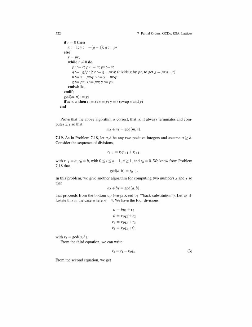
522 7 Partial Orders, GCDs, RSA, Lattices
if r = 0 thenx := 1; y :=−(q−1); g := pr
elser = pr;while r 6= 0 do
pr := r; pu := u; pv := v;q := bg/prc; r := g− pr q; (divide g by pr, to get g = pr q+ r)u := x− puq; v := y− pvq;g := pr; x := pu; y := pv
endwhile;endif;gcd(m,n) := g;if m < n then t := x; x = y; y = t (swap x and y)
end
Prove that the above algorithm is correct, that is, it always terminates and com-putes x,y so that
mx+ny = gcd(m,n),
7.19. As in Problem 7.18, let a,b be any two positive integers and assume a ≥ b.Consider the sequence of divisions,
ri−1 = riqi+1 + ri+1,
with r−1 = a, r0 = b, with 0≤ i≤ n−1, n≥ 1, and rn = 0. We know from Problem7.18 that
gcd(a,b) = rn−1.
In this problem, we give another algorithm for computing two numbers x and y sothat
ax+by = gcd(a,b),
that proceeds from the bottom up (we proceed by “‘back-substitution”). Let us il-lustate this in the case where n = 4. We have the four divisions:
a = bq1 + r1
b = r1q2 + r2
r1 = r2q3 + r3
r2 = r3q3 +0,
with r3 = gcd(a,b).From the third equation, we can write
r3 = r1− r2q3. (3)
From the second equation, we get
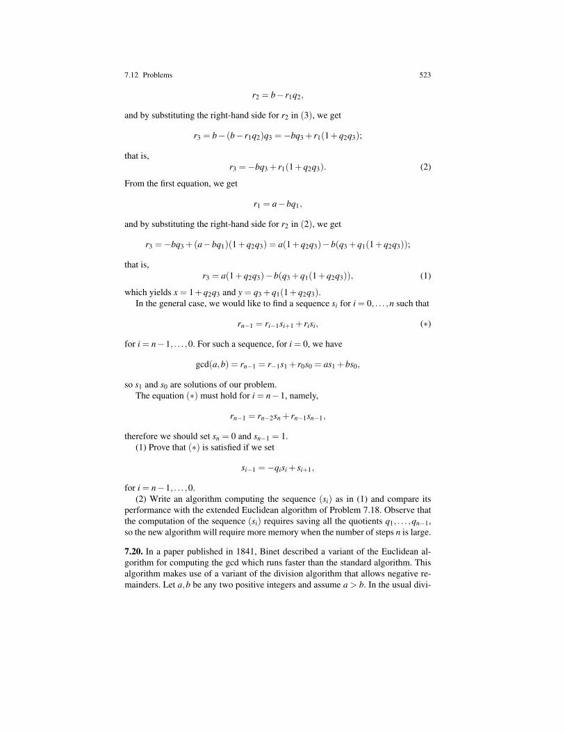
7.12 Problems 523
r2 = b− r1q2,
and by substituting the right-hand side for r2 in (3), we get
r3 = b− (b− r1q2)q3 =−bq3 + r1(1+q2q3);
that is,r3 =−bq3 + r1(1+q2q3). (2)
From the first equation, we get
r1 = a−bq1,
and by substituting the right-hand side for r2 in (2), we get
r3 =−bq3 +(a−bq1)(1+q2q3) = a(1+q2q3)−b(q3 +q1(1+q2q3));
that is,r3 = a(1+q2q3)−b(q3 +q1(1+q2q3)), (1)
which yields x = 1+q2q3 and y = q3 +q1(1+q2q3).In the general case, we would like to find a sequence si for i = 0, . . . ,n such that
rn−1 = ri−1si+1 + risi, (∗)
for i = n−1, . . . ,0. For such a sequence, for i = 0, we have
gcd(a,b) = rn−1 = r−1s1 + r0s0 = as1 +bs0,
so s1 and s0 are solutions of our problem.The equation (∗) must hold for i = n−1, namely,
rn−1 = rn−2sn + rn−1sn−1,
therefore we should set sn = 0 and sn−1 = 1.(1) Prove that (∗) is satisfied if we set
si−1 =−qisi + si+1,
for i = n−1, . . . ,0.(2) Write an algorithm computing the sequence (si) as in (1) and compare its
performance with the extended Euclidean algorithm of Problem 7.18. Observe thatthe computation of the sequence (si) requires saving all the quotients q1, . . . ,qn−1,so the new algorithm will require more memory when the number of steps n is large.
7.20. In a paper published in 1841, Binet described a variant of the Euclidean al-gorithm for computing the gcd which runs faster than the standard algorithm. Thisalgorithm makes use of a variant of the division algorithm that allows negative re-mainders. Let a,b be any two positive integers and assume a > b. In the usual divi-
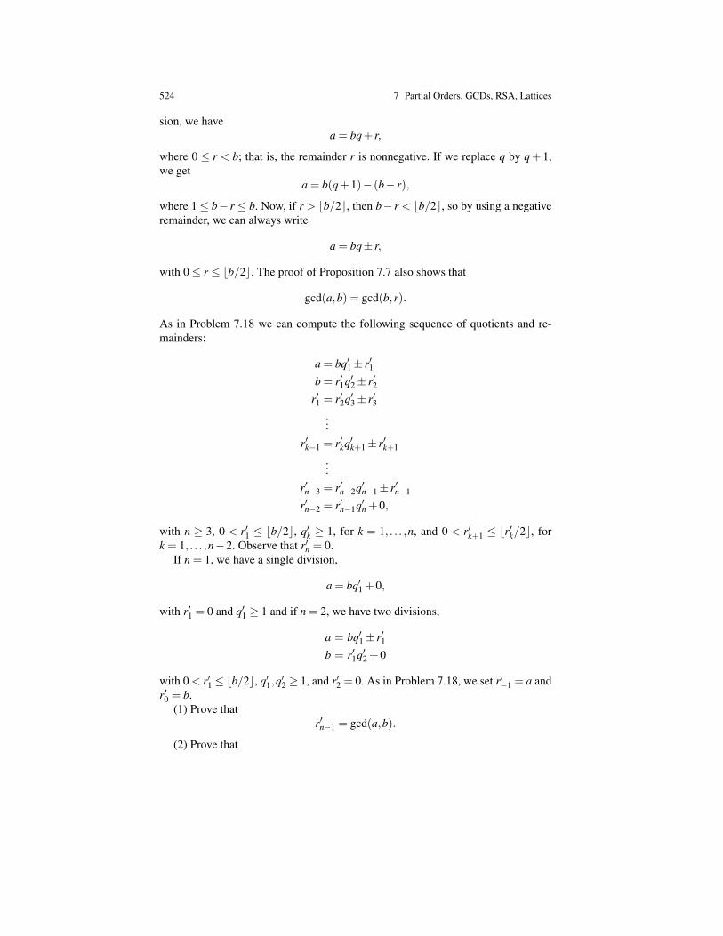
524 7 Partial Orders, GCDs, RSA, Lattices
sion, we havea = bq+ r,
where 0 ≤ r < b; that is, the remainder r is nonnegative. If we replace q by q+ 1,we get
a = b(q+1)− (b− r),
where 1≤ b− r ≤ b. Now, if r > bb/2c, then b− r < bb/2c, so by using a negativeremainder, we can always write
a = bq± r,
with 0≤ r ≤ bb/2c. The proof of Proposition 7.7 also shows that
gcd(a,b) = gcd(b,r).
As in Problem 7.18 we can compute the following sequence of quotients and re-mainders:
a = bq′1± r′1b = r′1q′2± r′2
r′1 = r′2q′3± r′3...
r′k−1 = r′kq′k+1± r′k+1
...r′n−3 = r′n−2q′n−1± r′n−1
r′n−2 = r′n−1q′n +0,
with n ≥ 3, 0 < r′1 ≤ bb/2c, q′k ≥ 1, for k = 1, . . . ,n, and 0 < r′k+1 ≤ br′k/2c, fork = 1, . . . ,n−2. Observe that r′n = 0.
If n = 1, we have a single division,
a = bq′1 +0,
with r′1 = 0 and q′1 ≥ 1 and if n = 2, we have two divisions,
a = bq′1± r′1b = r′1q′2 +0
with 0 < r′1 ≤ bb/2c, q′1,q′2 ≥ 1, and r′2 = 0. As in Problem 7.18, we set r′−1 = a and
r′0 = b.(1) Prove that
r′n−1 = gcd(a,b).
(2) Prove that
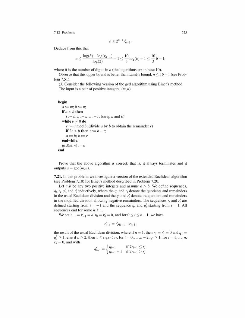
7.12 Problems 525
b≥ 2n−1r′n−1.
Deduce from this that
n≤ log(b)− log(rn−1)
log(2)+1≤ 10
3log(b)+1≤ 10
3δ +1,
where δ is the number of digits in b (the logarithms are in base 10).Observe that this upper bound is better than Lame’s bound, n≤ 5δ +1 (see Prob-
lem 7.51).(3) Consider the following version of the gcd algorithm using Binet’s method.The input is a pair of positive integers, (m,n).
begina := m; b := n;if a < b then
t := b; b := a; a := t; (swap a and b)while b 6= 0 do
r := a mod b; (divide a by b to obtain the remainder r)if 2r > b then r := b− r;a := b; b := r
endwhile;gcd(m,n) := a
end
Prove that the above algorithm is correct; that is, it always terminates and itoutputs a = gcd(m,n).
7.21. In this problem, we investigate a version of the extended Euclidean algorithm(see Problem 7.18) for Binet’s method described in Problem 7.20.
Let a,b be any two positive integers and assume a > b. We define sequences,qi,ri,q′i, and r′i inductively, where the qi and ri denote the quotients and remaindersin the usual Euclidean division and the q′i and r′i denote the quotient and remaindersin the modified division allowing negative remainders. The sequences ri and r′i aredefined starting from i = −1 and the sequence qi and q′i starting from i = 1. Allsequences end for some n≥ 1.
We set r−1 = r′−1 = a,r0 = r′0 = b, and for 0≤ i≤ n−1, we have
r′i−1 = r′iqi+1 + ri+1,
the result of the usual Euclidean division, where if n = 1, then r1 = r′1 = 0 and q1 =q′1 ≥ 1, else if n≥ 2, then 1≤ ri+1 < ri, for i = 0, . . . ,n−2, qi ≥ 1, for i = 1, . . . ,n,rn = 0, and with
q′i+1 =
qi+1 if 2ri+1 ≤ r′iqi+1 +1 if 2ri+1 > r′i

526 7 Partial Orders, GCDs, RSA, Lattices
and
r′i+1 =
ri+1 if 2ri+1 ≤ r′ir′i− ri+1 if 2ri+1 > r′i,
for i = 0, . . . ,n−1.(1) Check that
r′i−1 =
r′iq′i+1 + r′i+1 if 2ri+1 ≤ r′i
r′iq′i+1− r′i+1 if 2ri+1 > r′i
and prove thatr′n−1 = gcd(a,b).
(2) If n≥ 2, define the sequences, xi and yi inductively as follows:x−1 = 1,x0 = 0, y−1 = 0,y0 = 1,
xi+1 =
xi−1− xiq′i+1 if 2ri+1 ≤ r′ixiq′i+1− xi−1 if 2ri+1 > r′i
and
yi+1 =
yi−1− yiq′i+1 if 2ri+1 ≤ r′iyiq′i+1− yi−1 if 2ri+1 > r′i,
for i = 0, . . . ,n−2.Prove that if n≥ 2, then
axi +byi = r′i,
for i =−1, . . . ,n−1 and thus,
axn−1 +byn−1 = gcd(a,b) = r′n−1.
(3) Design an algorithm combining the algorithms proposed in Problems 7.18and 7.20.
7.22. (1) Let m1,m2 be any two positive natural numbers and assume that m1 andm2 are relatively prime.
Prove that for any pair of integers a1,a2 there is some integer x such that thefollowing two congruences hold simultaneously.
x ≡ a1 (mod m1)
x ≡ a2 (mod m2).
Furthermore, prove that if x and y are any two solutions of the above system, thenx≡ y (mod m1m2), so x is unique if we also require that 0≤ x < m1m2.Hint. By the Bezout identity (Proposition 7.6), there exist some integers, y1,y2, sothat
m1y1 +m2y2 = 1.
Prove that x = a1m2y2 + a2m1y1 = a1(1− m1y1) + a2m1y1 = a1m2y2 + a2(1−m2y2) works. For the second part, prove that if m1 and m2 both divide b and ifgcd(m1,m2) = 1, then m1m2 divides b.
7.12 Problems 527
(2) Let m1,m2, . . . ,mn be any n≥ 2 positive natural numbers and assume that themi are pairwise relatively prime, which means that mi and mi are relatively primefor all i 6= j.
Prove that for any n integers a1,a2, . . . ,an, there is some integer x such that thefollowing n congruences hold simultaneously.
x≡ a1 (mod m1)
x≡ a2 (mod m2)
...x≡ an (mod mn).
Furthermore, prove that if x and y are any two solutions of the above system, thenx≡ y(modm), where m = m1m2 · · ·mn, so x is unique if we also require that 0≤ x <m. The above result is known as the Chinese remainder theorem.Hint. Use induction on n. First, prove that m1 and m2 · · ·mn are relatively prime(because the mi are pairwise relatively prime). By (1), there exists some z1 so that
z1 ≡ 1 (mod m1)
z1 ≡ 0 (mod m2 · · ·mn).
By the induction hypothesis, there exists z2, . . . ,zn, so that
zi ≡ 1 (mod mi)
zi ≡ 0 (mod m j)
for all i = 2, . . . ,n and all j 6= i, with 2≤ j ≤ n; show that
x = a1z1 +a2z2 + · · ·+anzn
works.(3) Let m = m1 · · ·mn and let Mi = m/mi = ∏
nj=1, j 6=i m j, for i = 1, . . . ,n. As in
(2), we know that mi and Mi are relatively prime, thus by Bezout (or the extendedEuclidean algorithm), we can find some integers ui,vi so that
miui +Mivi = 1,
for i = 1, . . . ,n. If we let zi = Mivi = mvi/mi, then prove that
x = a1z1 + · · ·+anzn
is a solution of the system of congruences.
7.23. The Euler φ -function (or totient) is defined as follows. For every positive in-teger m, φ(m) is the number of integers, n ∈ 1, . . . ,m, such that m is relativelyprime to n. Observe that φ(1) = 1.
528 7 Partial Orders, GCDs, RSA, Lattices
(1) Prove the following fact. For every positive integer a, if a and m are relativelyprime, then
aφ(m) ≡ 1 (mod m);
that is, m divides aφ(m)−1.Hint. Let s1, . . . ,sk be the integers, si ∈ 1, . . . ,m, such that si is relatively primeto m (k = φ(m)). Let r1, . . . ,rk be the remainders of the divisions of s1a,s2a, . . . ,skaby m (so, sia = mqi + ri, with 0≤ ri < m).
(i) Prove that gcd(ri,m) = 1, for i = 1, . . . ,k.(ii) Prove that ri 6= r j whenever i 6= j, so that
r1, . . . ,rk= s1, . . . ,sk.
Use (i) and (ii) to prove that
aks1 · · ·sk ≡ s1 · · ·sk (mod m)
and use this to conclude that
aφ(m) ≡ 1 (mod m).
(2) Prove that if p is prime, then φ(p) = p−1 and thus, Fermat’s little theoremis a special case of (1).
7.24. Prove that if p is a prime, then for every integer x we have x2 ≡ 1 (mod p) iffx≡±1 (mod p).
7.25. For any two positive integers a,m prove that gcd(a,m) = 1 iff there is someinteger x so that ax≡ 1 (mod m).
7.26. Prove that if p is a prime, then
(p−1)!≡−1 (mod p).
This result is known as Wilson’s theorem.Hint. The cases p = 2 and p = 3 are easily checked, so assume p ≥ 5. Considerany integer a, with 1 ≤ a ≤ p− 1. Show that gcd(a, p) = 1. Then, by the result ofProblem 7.25, there is a unique integer a such that 1≤ a≤ p−1 and aa≡ 1(mod p).Furthermore, a is the unique integer such that 1 ≤ a ≤ p− 1 and aa ≡ 1 (mod p).Thus, the numbers in 1, . . . , p− 1 come in pairs a,a such that aa ≡ 1 (mod p).However, one must be careful because it may happen that a = a, which is equivalentto a2 ≡ 1 (mod p). By Problem 7.24, this happens iff a ≡ ±1 (mod p), iff a = 1 ora = p−1. By pairing residues modulo p, prove that
p−2
∏a=2
a≡ 1 (mod p)
and use this to prove that

7.12 Problems 529
(p−1)!≡−1 (mod p).
7.27. Let φ be the Euler-φ function defined in Problem 7.23.(1) Prove that for every prime p and any integer k ≥ 1 we have
φ(pk) = pk−1(p−1).(2) Prove that for any two positive integers m1,m2, if gcd(m1,m2) = 1, then
φ(m1m2) = φ(m1)φ(m2).
Hint. For any integer m≥ 1, let
R(m) = n ∈ 1, . . . ,m | gcd(m,n) = 1.
Let m = m1m2. For every n ∈R(m), if a1 is the remainder of the division of n bym1 and similarly if a2 is the remainder of the division of n by m2, then prove thatgcd(a1,m1) = 1 and gcd(a2,m2) = 1. Consequently, we get a function θ : R(m)→R(m1)×R(m1), given by θ(n) = (a1,a2).
Prove that for every pair (a1,a2) ∈R(m1)×R(m1), there is a unique n ∈R(m),so that θ(n) = (a1,a2) (Use the Chinese remainder theorem; see Problem 7.22).Conclude that θ is a bijection. Use the bijection θ to prove that
φ(m1m2) = φ(m1)φ(m2).
(3) Use (1) and (2) to prove that for every integer n ≥ 2, if n = pk11 · · · pkr
r is theprime factorization of n, then
φ(n) = pk1−11 · · · pkr−1
r (p1−1) · · ·(pr−1) = n(
1− 1p1
)· · ·(
1− 1pr
).
7.28. Prove that the function, f : N×N→ N, given by
f (m,n) = 2m(2n+1)−1
is a bijection.
7.29. Let S = a1, . . . ,an be any nonempty set of n positive natural numbers. Provethat there is a nonempty subset of S whose sum is divisible by n.Hint. Consider the numbers, b1 = a1, b2 = a1 +a2, . . . , bn = a1 +a2 + · · ·+an.
7.30. Establish the formula
A =
(1 11 0
)=
1√5
(ϕ −ϕ−1
1 1
)(ϕ 00 −ϕ−1
)(1 ϕ−1
−1 ϕ
)with ϕ = (1+
√5)/2 given in Section 7.6 and use it to prove that(un+1
un
)=
1√5
(ϕ −ϕ−1
1 1
)((ϕ−1u0 +u1)ϕ
n
(ϕu0−u1)(−ϕ−1)n
).
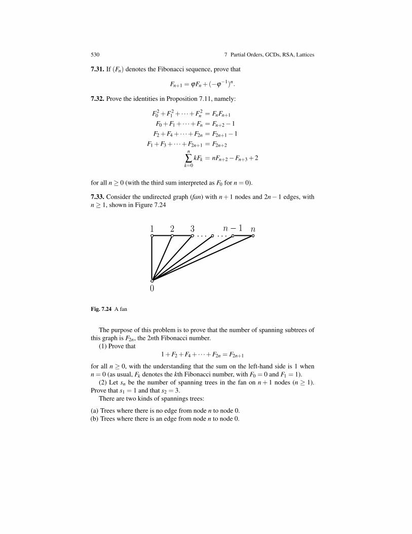
530 7 Partial Orders, GCDs, RSA, Lattices
7.31. If (Fn) denotes the Fibonacci sequence, prove that
Fn+1 = ϕFn +(−ϕ−1)n.
7.32. Prove the identities in Proposition 7.11, namely:
F20 +F2
1 + · · ·+F2n = FnFn+1
F0 +F1 + · · ·+Fn = Fn+2−1F2 +F4 + · · ·+F2n = F2n+1−1
F1 +F3 + · · ·+F2n+1 = F2n+2n
∑k=0
kFk = nFn+2−Fn+3 +2
for all n≥ 0 (with the third sum interpreted as F0 for n = 0).
7.33. Consider the undirected graph (fan) with n+ 1 nodes and 2n− 1 edges, withn≥ 1, shown in Figure 7.24
1
1 2 3 n ! 1 n
0
· · · · · ·
Fig. 7.24 A fan
The purpose of this problem is to prove that the number of spanning subtrees ofthis graph is F2n, the 2nth Fibonacci number.
(1) Prove that1+F2 +F4 + · · ·+F2n = F2n+1
for all n ≥ 0, with the understanding that the sum on the left-hand side is 1 whenn = 0 (as usual, Fk denotes the kth Fibonacci number, with F0 = 0 and F1 = 1).
(2) Let sn be the number of spanning trees in the fan on n+ 1 nodes (n ≥ 1).Prove that s1 = 1 and that s2 = 3.
There are two kinds of spannings trees:
(a) Trees where there is no edge from node n to node 0.(b) Trees where there is an edge from node n to node 0.
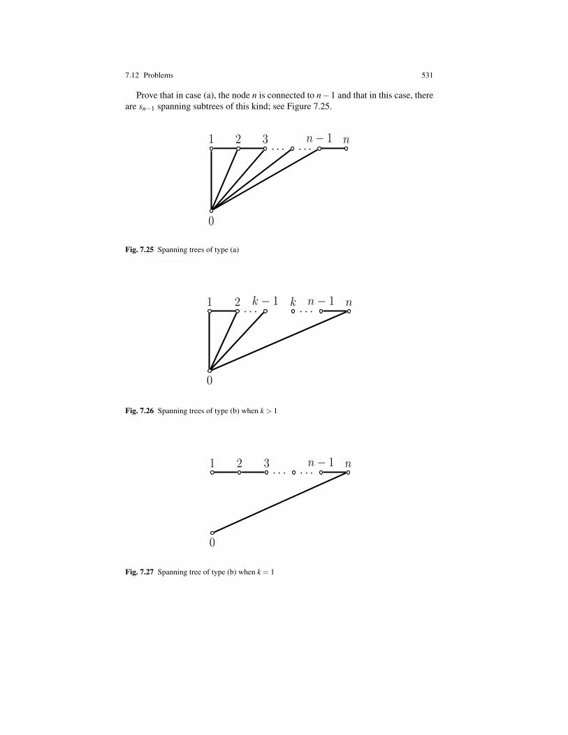
7.12 Problems 531
Prove that in case (a), the node n is connected to n−1 and that in this case, thereare sn−1 spanning subtrees of this kind; see Figure 7.25.
1
1 2 3 n ! 1 n
0
· · · · · ·
Fig. 7.25 Spanning trees of type (a)
1
1 2 k ! 1 k n ! 1 n
0
· · ·· · ·
Fig. 7.26 Spanning trees of type (b) when k > 1
1
1 2 3 n ! 1 n
0
· · · · · ·
Fig. 7.27 Spanning tree of type (b) when k = 1

532 7 Partial Orders, GCDs, RSA, Lattices
Observe that in case (b), there is some k ≤ n such that the edges between thenodes n,n− 1, . . . ,k are in the tree but the edge from k to k− 1 is not in the treeand that none of the edges from 0 to any node in n−1, . . . ,k are in this tree; seeFigure 7.26.
Furthermore, prove that if k = 1, then there is a single tree of this kind (see Figure7.27) and if k > 1, then there are
sn−1 + sn−2 + · · ·+ s1
trees of this kind.(3) Deduce from (2) that
sn = sn−1 + sn−1 + sn−2 + · · ·+ s1 +1,
with s1 = 1. Use (1) to prove that
sn = F2n,
for all n≥ 1.
7.34. Prove the Zeckendorf representation of natural numbers, that is, Proposition7.12.Hint. For the existence part, prove by induction on k ≥ 2 that a decomposition ofthe required type exists for all n ≤ Fk (with n ≥ 1). For the uniqueness part, firstprove that
F(n mod 2)+2 + · · ·+Fn−2 +Fn = Fn+1−1,
for all n≥ 2.
7.35. Prove Proposition 7.13 giving identities relating the Fibonacci numbers andthe Lucas numbers:
Ln = Fn−1 +Fn+1
5Fn = Ln−1 +Ln+1,
for all n≥ 1.
7.36. Prove Proposition 7.14; that is, for any fixed k ≥ 1 and all n≥ 0, we have
Fn+k = FkFn+1 +Fk−1Fn.
Use the above to prove thatF2n = FnLn,
for all n≥ 1.
7.37. Prove the following identities.
7.12 Problems 533
LnLn+2 = L2n+1 +5(−1)n
L2n = L2n−2(−1)n
L2n+1 = LnLn+1− (−1)n
L2n = 5F2
n +4(−1)n.
7.38. (a) Prove Proposition 7.15; that is,
un+1un−1−u2n = (−1)n−1(u2
0 +u0u1−u21).
(b) Prove the Catalan identity,
Fn+rFn−r−F2n = (−1)n−r+1F2
r , n≥ r.
7.39. Prove that any sequence defined by the recurrence
un+2 = un+1 +un
satisfies the following equation,
ukun+1 +uk−1un = u1un+k +u0un+k−1,
for all k ≥ 1 and all n≥ 0.
7.40. Prove Proposition 7.16; that is,
1. Fn divides Fmn, for all m,n≥ 1.2. gcd(Fm,Fn) = Fgcd(m,n), for all m,n≥ 1.
Hint. For the first statement, use induction on m ≥ 1. To prove the second statete-ment, first prove that
gcd(Fn,Fn+1) = 1
for all n≥ 1. Then, prove that
gcd(Fm,Fn) = gcd(Fm−n,Fn).
7.41. Prove the formulae
2Fm+n = FmLn +FnLm
2Lm+n = LmLn +5FmFn.
7.42. Prove that
L2h+1n = L(2h+1)n +
(2h+1
1
)(−1)nL(2h−1)n +
(2h+1
2
)(−1)2nL(2h−3)n + · · ·
+
(2h+1
h
)(−1)hnLn.
534 7 Partial Orders, GCDs, RSA, Lattices
7.43. Prove that
A =
(P −Q1 0
)=
1α−β
(α β
1 1
)(α 00 β
)(1 −β
−1 α
),
where
α =P+√
D2
, β =P−√
D2
and then prove that(un+1
un
)=
1α−β
(α β
1 1
)((−βu0 +u1)α
n
(αu0−u1)β n
).
7.44. Prove Proposition 7.17; that is, the sequence defined by the recurrence
un+2 = Pun+1−Qun
(with P2−4Q 6= 0) satisfies the identity:
un+1un−1−u2n = Qn−1(−Qu2
0 +Pu0u1−u21).
7.45. Prove the following identities relating the Un and the Vn;
Vn = Un+1−QUn−1
DUn = Vn+1−QVn−1,
for all n≥ 1. Then, prove that
U2n = UnVn
V2n = V 2n −2Qn
Um+n = UmUn+1−QUnUm−1
Vm+n = VmVn−QnVm−n.
7.46. Consider the recurrence
Vn+2 = 2Vn+1 +2Vn,
starting from V0 =V1 = 2. Prove that
Vn = (1+√
3)n +(1−√
3)n.
7.47. Consider the sequence Sn given by
Sn+1 = S2n−2,
starting with S0 = 4. Prove that
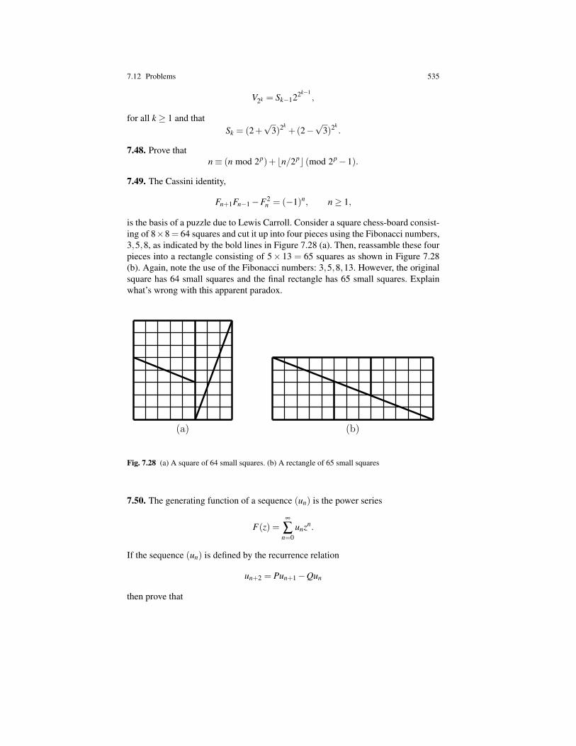
7.12 Problems 535
V2k = Sk−122k−1,
for all k ≥ 1 and thatSk = (2+
√3)2k
+(2−√
3)2k.
7.48. Prove thatn≡ (n mod 2p)+ bn/2pc (mod 2p−1).
7.49. The Cassini identity,
Fn+1Fn−1−F2n = (−1)n, n≥ 1,
is the basis of a puzzle due to Lewis Carroll. Consider a square chess-board consist-ing of 8×8 = 64 squares and cut it up into four pieces using the Fibonacci numbers,3,5,8, as indicated by the bold lines in Figure 7.28 (a). Then, reassamble these fourpieces into a rectangle consisting of 5× 13 = 65 squares as shown in Figure 7.28(b). Again, note the use of the Fibonacci numbers: 3,5,8,13. However, the originalsquare has 64 small squares and the final rectangle has 65 small squares. Explainwhat’s wrong with this apparent paradox.
1
(a) (b)
Fig. 7.28 (a) A square of 64 small squares. (b) A rectangle of 65 small squares
7.50. The generating function of a sequence (un) is the power series
F(z) =∞
∑n=0
unzn.
If the sequence (un) is defined by the recurrence relation
un+2 = Pun+1−Qun
then prove that
536 7 Partial Orders, GCDs, RSA, Lattices
F(z) =u0 +(u1−Pu0)z
1−Pz+Qz2 .
For the Fibonacci-style sequence u0 = 0, u1 = 1, so we have
FFib(z) =z
1−Pz+Qz2
and for the Lucas-style sequence u0 = 2, u1 = 1, so we have
FLuc(z) =2+(1−2P)z1−Pz+Qz2 .
If Q 6= 0, prove that
F(z) =1
α−β
(−βu0 +u1
1−αz+
αu0−u1
1−β z
).
Prove that the above formula for F(z) yields, again,
un =1
α−β
((−βu0 +u1)α
n +(αu0−u1)βn).
Prove that the above formula is still valid for Q= 0, provided we assume that 00 = 1.
7.51. (1) Prove that the Euclidean algorithm for gcd applied to two consecutive Fi-bonacci numbers Fn and Fn+1 (with n≥ 2) requires n−1 divisions.
(2) Prove that the Euclidean algorithm for gcd applied to two consecutive Lucasnumbers Ln and Ln+1 (with n≥ 1) requires n divisions.
(3) Prove that if a > b ≥ 1 and if the Euclidean algorithm for gcd applied to aand b requires n divisions, then a≥ Fn+2 and b≥ Fn+1.
(4) Using the explicit formula for Fn+1 and by taking logarithms in base 10, use(3) to prove that
n < 4.785δ +1,
where δ is the number of digits in b (Dupre’s bound). This is slightly better thanLame’s bound, n≤ 5δ +1.
7.52. (1) Prove the correctness of the algorithm for computing xn mod m using re-peated squaring.
(2) Use your algorithm to check that the message sent to Albert has been de-crypted correctly and then encrypt the decrypted message and check that it is iden-tical to the original message.
7.53. Recall the recurrence relations given in Section 7.7 to compute the inversemodulo m of an integer a such that 1≤ a < m and gcd(m,a) = 1:
7.12 Problems 537
y−1 = 0y0 = 1
zi+1 = yi−1− yiqi+1
yi+1 = zi+1 mod m if zi+1 ≥ 0yi+1 = m− ((−zi+1)mod m) if zi+1 < 0,
for i = 0, . . . ,n−2.(1) Prove by induction that
ayi ≡ ri (mod m)
for i = 0, . . . ,n−1 and thus, that
ayn−1 ≡ 1 (mod m),
with 1≤ yn−1 < m, as desired.(2) Prove the correctness of the algorithm for computing the inverse of an element
modulo m proposed in Section 7.7.(3) Design a faster version of this algorithm using “Binet’s trick” (see Problem
7.20 and Problem 7.21).
7.54. Prove that a560− 1 is divisible by 561 for every positive natural number, a,such that gcd(a,561) = 1.Hint. Because 561= 3 ·11 ·17, it is enough to prove that 3 | (a560−1) for all positiveintegers a such that a is not a multiple of 3, that 11 | (a560−1) for all positive integersa such that a is not a multiple of 11, and that 17 | (a560−1) for all positive integersa such that a is not a multiple of 17.
7.55. Prove that 161038 divides 2161038−2, yet 2161037 ≡ 80520 (mod 161038).This example shows that it would be undesirable to define a pseudo-prime as a
positive natural number n that divides 2n−2.
7.56. (a) Consider the sequence defined recursively as follows.
U0 = 0U1 = 2
Un+2 = 6Un+1−Un, n≥ 0.
Prove the following identity,
Un+2Un =U2n+1−4,
for all n≥ 0.(b) Consider the sequence defined recursively as follows:
538 7 Partial Orders, GCDs, RSA, Lattices
V0 = 1V1 = 3
Vn+2 = 6Vn+1−Vn, n≥ 0.
Prove the following identity,
Vn+2Vn =V 2n+1 +8,
for all n≥ 0.(c) Prove that
V 2n −2U2
n = 1,
for all n≥ 0.Hint. Use (a) and (b). You may also want to prove by simultaneous induction that
V 2n −2U2
n = 1VnVn−1−2UnUn−1 = 3,
for all n≥ 1.
7.57. Consider the sequences (Un) and (Vn), given by the recurrence relations
U0 = 0V0 = 1U1 = y1
V1 = x1
Un+2 = 2x1Un+1−Un
Vn+2 = 2x1Vn+1−Vn,
for any two positive integers x1,y1.(1) If x1 and y1 are solutions of the (Pell) equation
x2−dy2 = 1,
where d is a positive integer that is not a perfect square, then prove that
V 2n −dU2
n = 1VnVn−1−dUnUn−1 = x1,
for all n≥ 1.(2) Verify that
Un =(x1 + y1
√d)n− (x1− y1
√d)n
2√
d
Vn =(x1 + y1
√d)n +(x1− y1
√d)n
2.
References 539
Deduce from this thatVn +Un
√d = (x1 + y1
√d)n.
(3) Prove that the Uns and Vns also satisfy the following simultaneous recurrencerelations:
Un+1 = x1Un + y1Vn
Vn+1 = dy1Un + x1Vn,
for all n≥ 0. Use the above to prove that
Vn+1 +Un+1√
d = (Vn +Un√
d)(x1 + y1√
d)
Vn+1−Un+1√
d = (Vn−Un√
d)(x1− y1√
d)
for all n≥ 0 and then that
Vn +Un√
d = (x1 + y1√
d)n
Vn−Un√
d = (x1− y1√
d)n
for all n ≥ 0. Use the above to give another proof of the formulae for Un and Vn in(2).
Remark: It can be shown that Pell’s equation,
x2−dy2 = 1,
where d is not a perfect square, always has solutions in positive integers. If (x1,y1) isthe solution with smallest x1 > 0, then every solution is of the form (Vn,Un), whereUn and Vn are defined in (1). Curiously, the “smallest solution” (x1,y1) can involvesome very large numbers. For example, it can be shown that the smallest positivesolution of
x2−61y2 = 1
is (x1,y1) = (1766319049,226153980).
7.58. Prove that every totally ordered poset is a distributive lattice. Prove that thelattice N+ under the divisibility ordering is a distributive lattice.
7.59. Prove part (b) of Proposition 7.16.
7.60. Prove that every finite distributive lattice is a Heyting algebra.
References
1. Garrett Birkhoff. Lattice Theory. Colloquium Publications, Vol. XXV. Providence, RI: AMS,third edition, 1973.
540 7 Partial Orders, GCDs, RSA, Lattices
2. Richard Crandall and Carl Pomerance. Prime Numbers. A Computational Perspective. NewYork: Springer, second edition, 2005.
3. H. Davenport. The Higher Arithmetic. An Introduction to the Theory of Numbers. Cambridge,UK: Cambridge University Press, eighth edition, 2008.
4. Martin Dietzfelbinger. Primality Testing in Polynomial Time: From Randomized Algorithmsto “Primes Is in P”. LNCS No. 3000. New York: Springer Verlag, first edition, 2004.
5. Peter Gustav Lejeune Dirichlet. Lectures on Number Theory, volume 16 of History of Math-ematics. Providence, RI: AMS, first edition, 1999.
6. Herbert B. Enderton. Elements of Set Theory. New York: Academic Press, first edition, 1977.7. Ronald L. Graham, Donald E. Knuth, and Oren Patashnik. Concrete Mathematics: A Foun-
dation For Computer Science. Reading, MA: Addison Wesley, second edition, 1994.8. Donald E. Knuth. The Art of Computer Programming, Volume 2: Seminumerical Algorithms.
Reading, MA: Addison Wesley, third edition, 1997.9. Neal Koblitz. A Course in Number Theory and Cryptography. GTM No. 114. New York:
Springer Verlag, second edition, 1994.10. L. Lovasz, J. Pelikan, and K. Vesztergombi. Discrete Mathematics. Elementary and Beyond.
Undergraduate Texts in Mathematics. New York: Springer, first edition, 2003.11. Alfred J. Menezes, Paul C. van Oorschot, and Scott A. Vanstone. Handbook of Applied
Cryptography. Boca Raton, FL: CRC Press, fifth edition, 2001.12. Ivan Niven, Herbert S. Zuckerman, and Hugh L. Montgomery. An Introduction to the Theory
of Numbers. New York: Wiley, fifth edition, 1991.13. Paulo Ribenboim. The Little Book of Bigger Primes. New York: Springer-Verlag, second
edition, 2004.14. R.L. Rivest, A. Shamir, and L. Adleman. A method for obtaining digital signatures and
public-key cryptosystems. Communications of the ACM, 21(2):120–126, 1978.15. Joseph H. Silverman. A Friendly Introduction to Number Theory. Upper Saddle River, NJ:
Prentice Hall, third edition, 2006.16. Patrick Suppes. Axiomatic Set Theory. New York: Dover, first edition, 1972.17. Andre Weil. Number Theory. An Approach Through History from Hammurapi to Legendre.
Boston: Birkhauser, first edition, 1987.
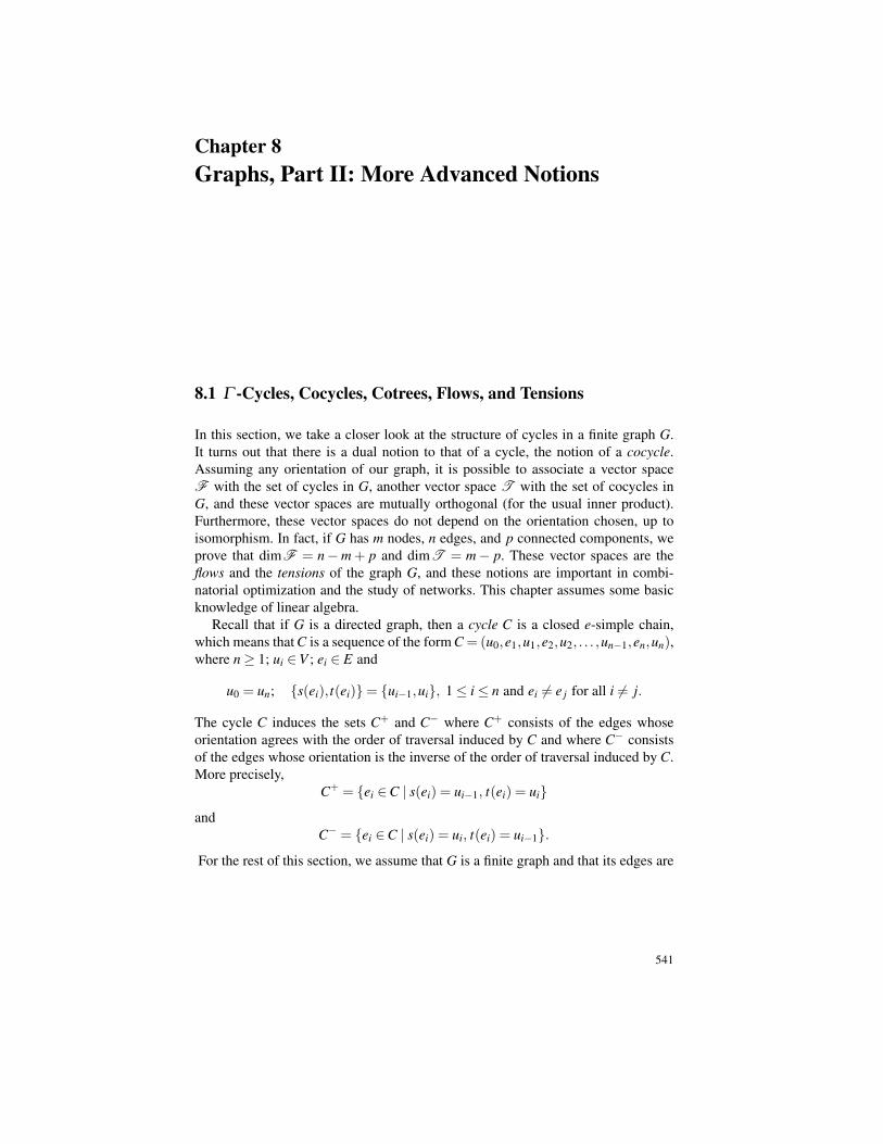
Chapter 8Graphs, Part II: More Advanced Notions
8.1 Γ -Cycles, Cocycles, Cotrees, Flows, and Tensions
In this section, we take a closer look at the structure of cycles in a finite graph G.It turns out that there is a dual notion to that of a cycle, the notion of a cocycle.Assuming any orientation of our graph, it is possible to associate a vector spaceF with the set of cycles in G, another vector space T with the set of cocycles inG, and these vector spaces are mutually orthogonal (for the usual inner product).Furthermore, these vector spaces do not depend on the orientation chosen, up toisomorphism. In fact, if G has m nodes, n edges, and p connected components, weprove that dimF = n−m+ p and dimT = m− p. These vector spaces are theflows and the tensions of the graph G, and these notions are important in combi-natorial optimization and the study of networks. This chapter assumes some basicknowledge of linear algebra.
Recall that if G is a directed graph, then a cycle C is a closed e-simple chain,which means that C is a sequence of the form C = (u0,e1,u1,e2,u2, . . . ,un−1,en,un),where n≥ 1; ui ∈V ; ei ∈ E and
u0 = un; s(ei), t(ei)= ui−1,ui, 1≤ i≤ n and ei 6= e j for all i 6= j.
The cycle C induces the sets C+ and C− where C+ consists of the edges whoseorientation agrees with the order of traversal induced by C and where C− consistsof the edges whose orientation is the inverse of the order of traversal induced by C.More precisely,
C+ = ei ∈C | s(ei) = ui−1, t(ei) = uiand
C− = ei ∈C | s(ei) = ui, t(ei) = ui−1.For the rest of this section, we assume that G is a finite graph and that its edges are
541
542 8 Graphs, Part II: More Advanced Notions
1
v4
v5
v1 v2
v3
e1
e7
e2 e3 e4
e5
e6
Fig. 8.1 Graph G8
named, e1, . . . ,en1.
Definition 8.1. Given any finite directed graph G with n edges, with every cycle Cis associated a representative vector γ(C) ∈ Rn, defined so that for every i, with1≤ i≤ n,
γ(C)i =
+1 if ei ∈C+
−1 if ei ∈C−
0 if ei /∈C.
For example, if G = G8 is the graph of Figure 8.1, the cycle
C = (v3,e7,v4,e6,v5,e5,v2,e1,v1,e2,v3)
corresponds to the vector
γ(C) = (−1,1,0,0,−1,−1,1).
Observe that distinct cycles may yield the same representative vector unless they aresimple cycles. For example, the cycles
C1 = (v2,e5,v5,e6,v4,e4,v2,e1,v1,e2,v3,e3,v2)
andC2 = (v2,e1,v1,e2,v3,e3,v2,e5,v5,e6,v4,e4,v2)
yield the same representative vector
γ = (−1,1,1,1,1,1,0).
In order to obtain a bijection between representative vectors and “cycles”, weintroduce the notion of a “Γ -cycle” (some authors redefine the notion of cycle andcall “cycle” what we call a Γ -cycle, but we find this practice confusing).
1 We use boldface notation for the edges in E in order to avoid confusion with the edges occurringin a cycle or in a chain; those are denoted in italic.
8.1 Γ -Cycles, Cocycles, Cotrees, Flows, and Tensions 543
Definition 8.2. Given a finite directed graph G = (V,E,s, t), a Γ -cycle is any setof edges Γ = Γ + ∪Γ− such that there is some cycle C in G with Γ + = C+ andΓ− =C−; we say that the cycle C induces the Γ -cycle, Γ . The representative vectorγ(Γ ) (for short, γ) associated with Γ is the vector γ(C) from Definition 8.1, whereC is any cycle inducing Γ . We say that a Γ -cycle Γ is a Γ -circuit iff either Γ + = /0or Γ− = /0 and that Γ is simple iff Γ arises from a simple cycle.
Remarks:
1. Given a Γ -cycle Γ = Γ + ∪Γ− we have the subgraphs G+ = (V,Γ +,s, t) andG− = (V,Γ−,s, t). Then, for every u ∈V , we have
d+G+(u)−d−G+(u)−d+
G−(u)+d−G−(u) = 0.
2. If Γ is a simple Γ -cycle, then every vertex of the graph (V,Γ ,s, t) has degree 0or 2.
3. When the context is clear and no confusion may arise, we often drop the “Γ ” inΓ -cycle and simply use the term “cycle”.
Proposition 8.1. If G is any finite directed graph, then any Γ -cycle Γ is the disjointunion of simple Γ -cycles.
Proof . This is an immediate consequence of Proposition 4.6. ut
Corollary 8.1. If G is any finite directed graph, then any Γ -cycle Γ is simple iff itis minimal, that is, if there is no Γ -cycle Γ ′ such that Γ ′ ⊆ Γ and Γ ′ 6= Γ .
We now consider a concept that turns out to be dual to the notion of Γ -cycle.
Definition 8.3. Let G be a finite directed graph G = (V,E,s, t) with n edges. For anysubset of nodes Y ⊆V , define the sets of edges Ω+(Y ) and Ω−(Y ) by
Ω+(Y ) = e ∈ E | s(e) ∈ Y, t(e) /∈ Y
Ω−(Y ) = e ∈ E | s(e) /∈ Y, t(e) ∈ Y
Ω(Y ) = Ω+(Y )∪Ω
−(Y ).
Any set Ω of edges of the form Ω = Ω(Y ), for some set of nodes Y ⊆ V , is calleda cocycle (or cutset). With every cocycle Ω we associate the representative vectorω(Ω) ∈ Rn defined so that
ω(Ω)i =
+1 if ei ∈Ω+
−1 if ei ∈Ω−
0 if ei /∈Ω ,
with 1≤ i≤ n. We also write ω(Y ) for ω(Ω) when Ω = Ω(Y ). If either Ω+(Y ) = /0or Ω−(Y ) = /0, then Ω is called a cocircuit and a simple cocycle (or bond) is aminimal cocycle (i.e., there is no cocycle Ω ′ such that Ω ′ ⊆Ω and Ω ′ 6= Ω ).
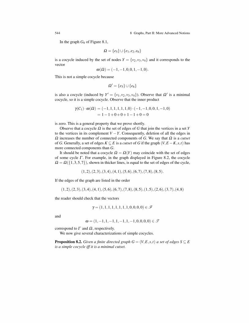
544 8 Graphs, Part II: More Advanced Notions
In the graph G8 of Figure 8.1,
Ω = e5∪e1,e2,e6
is a cocycle induced by the set of nodes Y = v2,v3,v4 and it corresponds to thevector
ω(Ω) = (−1,−1,0,0,1,−1,0).
This is not a simple cocycle because
Ω′ = e5∪e6
is also a cocycle (induced by Y ′ = v1,v2,v3,v4). Observe that Ω ′ is a minimalcocycle, so it is a simple cocycle. Observe that the inner product
γ(C1) ·ω(Ω) = (−1,1,1,1,1,1,0) · (−1,−1,0,0,1,−1,0)= 1−1+0+0+1−1+0 = 0
is zero. This is a general property that we prove shortly.Observe that a cocycle Ω is the set of edges of G that join the vertices in a set Y
to the vertices in its complement V −Y . Consequently, deletion of all the edges inΩ increases the number of connected components of G. We say that Ω is a cutsetof G. Generally, a set of edges K ⊆ E is a cutset of G if the graph (V,E−K,s, t) hasmore connected components than G.
It should be noted that a cocycle Ω = Ω(Y ) may coincide with the set of edgesof some cycle Γ . For example, in the graph displayed in Figure 8.2, the cocycleΩ = Ω(1,3,5,7), shown in thicker lines, is equal to the set of edges of the cycle,
(1,2),(2,3),(3,4),(4,1),(5,6),(6,7),(7,8),(8,5).
If the edges of the graph are listed in the order
(1,2),(2,3),(3,4),(4,1),(5,6),(6,7),(7,8),(8,5),(1,5),(2,6),(3,7),(4,8)
the reader should check that the vectors
γ = (1,1,1,1,1,1,1,1,0,0,0,0) ∈F
andω = (1,−1,1,−1,1,−1,1,−1,0,0,0,0) ∈T
correspond to Γ and Ω , respectively.We now give several characterizations of simple cocycles.
Proposition 8.2. Given a finite directed graph G = (V,E,s, t) a set of edges S ⊆ Eis a simple cocycle iff it is a minimal cutset.

8.1 Γ -Cycles, Cocycles, Cotrees, Flows, and Tensions 545
1
1 2
34
5 6
78
Fig. 8.2 A cocycle Ω equal to the edge set of a cycle Γ
Proof . We already observed that every cocycle is a cutset. Furthermore, we claimthat every cutset contains a cocyle. To prove this, it is enough to consider a minimalcutset S and to prove the following satement.
Claim. Any minimal cutset S is the set of edges of G that join two nonempty setsof vertices Y1 and Y2 such that
(i) Y1∩Y2 = /0.(ii) Y1∪Y2 =C, some connected component of G.
(iii) The subgraphs GY1 and GY2 , induced by Y1 and Y2 are connected.
Indeed, if S is a minimal cutset, it disconnects a unique connected component ofG, say C. Let C1, . . . ,Ck be the connected components of the graph C−S, obtainedfrom C by deleting the edges in S. Adding any edge e ∈ S to C− S must connecttwo components of C because otherwise S−e would disconnect C, contradictingthe minimality of C. Furthermore, k = 2, because otherwise, again, S−e woulddisconnect C. Then, if Y1 is the set of nodes of C1 and Y2 is the set of nodes of C2, itis clear that the claim holds.
Now, if S is a minimal cutset, the above argument shows that S contains a cocyleand this cocycle must be simple (i.e., minimal as a cocycle) as it is a cutset. Con-versely, if S is a simple cocycle (i.e., minimal as a cocycle), it must be a minimalcutset because otherwise, S would contain a strictly smaller cutset which would thencontain a cocycle strictly contained in S. ut
Proposition 8.3. Given a finite directed graph G = (V,E,s, t) a set of edges S⊆ E isa simple cocycle iff S is the set of edges of G that join two nonempty sets of verticesY1 and Y2 such that
(i) Y1∩Y2 = /0.(ii) Y1∪Y2 =C, some connected component of G.
(iii) The subgraphs GY1 and GY2 , induced by Y1 and Y2 are connected.
546 8 Graphs, Part II: More Advanced Notions
Proof . It is clear that if S satisfies (i)–(iii), then S is a minimal cutset and by Propo-sition 8.3, it is a simple cocycle.
Let us first assume that G is connected and that S=Ω(Y ) is a simple cocycle; thatis, is minimal as a cocycle. If we let Y1 = Y and Y2 = X −Y1, it is clear that (i) and(ii) are satisfied. If GY1 or GY2 is not connected, then if Z is a connected componentof one of these two graphs, we see that Ω(Z) is a cocycle strictly contained inS = Ω(Y1), a contradiction. Therefore, (iii) also holds. If G is not connected, as S isa minimal cocycle it is a minimal cutset, and so it is contained in some connectedcomponent C of G and we apply the above argument to C. ut
The following proposition is the analogue of Proposition 8.1 for cocycles.
Proposition 8.4. Given a finite directed graph G = (V,E,s, t), every cocycle Ω =Ω(Y ) is the disjoint union of simple cocycles.
Proof . We give two proofs.Proof 1: (Claude Berge) Let Y1, . . . ,Yk be the connected components of the subgraphof G induced by Y . Then, it is obvious that
Ω(Y ) = Ω(Y1)∪·· ·∪Ω(Yk),
where the Ω(Yi) are pairwise disjoint. So, it is enough to show that each Ω(Yi) isthe union of disjoint simple cycles.
Let C be the connected component of G that contains Yi and let C1, . . . ,Cm bethe connected components of the subgraph C−Y , obtained from C by deleting thenodes in Yi and the edges incident to these nodes. Observe that the set of edges thatare deleted when the nodes in Yi are deleted is the union of Ω(Yi) and the edges ofthe connected subgraph induced by Yi. As a consequence, we see that
Ω(Yi) = Ω(C1)∪·· ·∪Ω(Cm),
where Ω(Ck) is the set of edges joining Ck and nodes from Yi in the connectedsubgraph induced by the nodes in Yi∪
⋃j 6=k C j. By Proposition 8.3, the set Ω(Ck) is
a simple cocycle and it is clear that the sets Ω(Ck) are pairwise disjoint inasmuchas the Ck are disjoint.Proof 2: (Michel Sakarovitch) Let Ω = Ω(Y ) be a cocycle in G. Now, Ω is acutset and we can pick some minimal cocycle Ω1 = Ω(Z) contained in Ω . Weproceed by induction on |Ω −Ω1|. If Ω = Ω1, we are done. Otherwise, we claimthat E1 = Ω −Ω1 is a cutset in G. If not, let e be any edge in E1; we may assumethat a = s(e) ∈Y and b = t(e) ∈V −Y . As E1 is not a cutset, there is a chain C froma to b in (V,E−E1,s, t) and as Ω is a cutset, this chain must contain some edge e′ inΩ , so C =C1(x,e′,y)C2, where C1 is a chain from a to x and C2 is a chain from y tob. Then, because C has its edges in E−E1 and E1 = Ω−Ω1, we must have e′ ∈Ω1.We may assume that x = s(e′) ∈ Z and y = t(e′) ∈ V −Z. But, we have the chainCR
1 (a,e,b)CR2 joining x and y in (V,E−Ω1), a contradiction. Therefore, E1 is indeed
a cutset of G. Now, there is some minimal cocycle Ω2 contained in E1. If Ω2 = E1,
8.1 Γ -Cycles, Cocycles, Cotrees, Flows, and Tensions 547
we are done. Otherwise, if we let E2 = E1−Ω2, we can show as we just did that E2is a cutset of G with |E2|< |E1. Thus, we finish the proof by applying the inductionhypothesis to E2. ut
We now prove the key property of orthogonality between cycles and cocycles.
Proposition 8.5. Given any finite directed graph G = (V,E,s, t), if γ = γ(C) is therepresentative vector of any Γ -cycle Γ = Γ (C) and ω = ω(Y ) is the representativevector of any cocycle, Ω = Ω(Y ), then
γ ·ω =n
∑i=1
γiωi = 0;
that is, γ and ω are orthogonal. (Here, |E|= n.)
Proof . Recall that Γ =C+∪C−, where C is a cycle in G, say
C = (u0,e1,u1, . . . ,uk−1,ek,uk), with uk = u0.
Then, by definition, we see that
γ ·ω = |C+∩Ω+(Y )|− |C+∩Ω
−(Y )|− |C−∩Ω+(Y )|+ |C−∩Ω
−(Y )|. (∗)
As we traverse the cycle C, when we traverse the edge ei between ui−1 and ui (1 ≤i≤ k), we note that
ei ∈ (C+∩Ω+(Y ))∪ (C−∩Ω
−(Y )) iff ui−1 ∈ Y, ui ∈V −Y
ei ∈ (C+∩Ω−(Y ))∪ (C−∩Ω
+(Y )) iff ui−1 ∈V −Y, ui ∈ Y.
In other words, every time we traverse an edge coming out from Y , its contributionto (∗) is +1 and every time we traverse an edge coming into Y its contribution to(∗) is −1. After traversing the cycle C entirely, we must have come out from Y asmany times as we came into Y , so these contributions must cancel out. ut.
Note that Proposition 8.5 implies that |Γ ∩Ω | is even.
Definition 8.4. Given any finite digraph G = (V,E,s, t), where E = e1, . . . ,en, thesubspace F (G) of Rn spanned by all vectors γ(Γ ), where Γ is any Γ -cycle, is calledthe cycle space of G or flow space of G and the subspace T (G) of Rn spanned by allvectors ω(Ω), where Ω is any cocycle, is called the cocycle space of G or tensionspace of G (or cut space of G).
When no confusion is possible, we write F for F (G) and T for T (G). Thus, Fis the space consisting of all linear combinations ∑
ki=1 αiγi of representative vectors
of Γ -cycles γi, and T is the the space consisting of all linear combinations ∑ki=1 αiωi
of representative vectors of cocycles ωi with αi ∈ R. Proposition 8.5 says that thespaces F and T are mutually orthogonal. Observe that Rn is isomorphic to the vec-tor space of functions f : E→R. Consequently, a vector f = ( f1, . . . , fn) ∈Rn may
548 8 Graphs, Part II: More Advanced Notions
be viewed as a function from E = e1, . . . ,en to R and it is sometimes convenientto write f (ei) instead of fi.
Remark: The seemingly odd terminology “flow space” and “tension space” is ex-plained later.
Our next goal is be to determine the dimensions of F and T in terms of thenumber of edges, the number of nodes, and the number of connected components ofG, and to give a convenient method for finding bases of F and T . For this, we usespanning trees and their dual, cotrees. But first, we need a crucial theorem that alsoplays an important role in the theory of flows in networks.
Theorem 8.1. (Arc Coloring Lemma; Minty [1960]) Let G = (V,E,s, t) be a finitedirected graph and assume that the edges of G are colored either in black, red, orgreen. Pick any edge e and color it black. Then, exactly one of two possibilities mayoccur:
(1) There is a simple cycle containing e whose edges are only red or black with allthe black edges oriented in the same direction.
(2) There is a simple cocycle containing e whose edges are only green or black withall the black edges oriented in the same direction.
Proof . Let a= s(e) and b= t(e). Apply the following procedure for marking nodes.
Intitially, only b is marked.while there is some marked node x and some unmarked node y with
either a black edge, e′, with (x,y) = (s(e′), t(e′)) ora red edge, e′, with (x,y) = s(e′), t(e′)then mark y; arc(y) = e′
endwhile
When the marking algorithm stops, exactly one of the following two cases oc-curs.
(i) Node a has been marked. Let e′ = arc(a) be the edge that caused a to be markedand let x be the other endpoint of e′. If x = b, we found a simple cycle satisfying(i). If not, let e′′ = arc(x) and let y be the other endpoint of e′′ and continue inthe same manner. This procedure will stop with b and yields the chain C from bto a along which nodes have been marked. This chain must be simple becauseevery edge in it was used once to mark some node (check that the set of edgesused for the marking is a tree). If we add the edge e to the chain C, we obtain asimple cycle Γ whose edges are colored black or red and with all edges coloredblack oriented in the same direction due to the marking scheme. It is impossibleto have a cocycle whose edges are colored black or green containing e becauseit would have been impossible to conduct the marking through this cocycle anda would not have been marked.

8.1 Γ -Cycles, Cocycles, Cotrees, Flows, and Tensions 549
(ii) Node a has not been marked. Let Y be the set of unmarked nodes. The set Ω(Y )is a cocycle whose edges are colored green or black containing e with all blackedges in Ω+(Y ). This cocycle is the disjoint of simple cocycles (by Proposition8.4) and one of these simple cocycles contains e. If a cycle with black or rededges containing e with all black edges oriented in the same direction existed,then a would have been marked, a contradiction. ut
Corollary 8.2. Every edge of a finite directed graph G belongs either to a simplecircuit or to a simple cocircuit but not both.
Proof . Color all edges black and apply Theorem 8.1. ut
Although Minty’s theorem looks more like an amusing fact than a deep result,it is actually a rather powerful theorem. For example, we show in Section 8.4 thatMinty’s theorem can be used to prove the “hard part” of the max-flow min-cut the-orem (Theorem 8.7), an important theorem that has many applications. Here are afew more applications of Theorem 8.1.
Proposition 8.6. Let G be a finite connected directed graph with at least one edge.Then, the following conditions are equivalent.
(i) G is strongly connected.(ii) Every edge belongs to some circuit.
(iii) G has no cocircuit.
Proof . (i) =⇒ (ii). If x and y are the endpoints of any edge e in G, as G is stronglyconnected, there is a simple path from y to x and thus, a simple circuit through e.
(ii) =⇒ (iii). This follows from Corollary 8.2.(iii) =⇒ (i). Assume that G is not strongly connected and let Y ′ and Y ′′ be two
strongly connected components linked by some edge e and let a = s(e) and b =t(e), with a ∈ Y ′ and b ∈ Y ′′. The edge e does not belong to any circuit becauseotherwise a and b would belong to the same strongly connected component. Thus,by Corollary 8.2, the edge e should belong to some cocircuit, a contradiction. ut
In order to determine the dimension of the cycle space T , we use spanning trees.Let us assume that G is connected because otherwise the same reasoning applies tothe connected components of G. If T is any spanning tree of G, we know fromTheorem 4.2, Part (4), that adding any edge e ∈ E−T (called a chord of T ) createsa (unique) cycle. We show shortly that the vectors associated with these cycles forma basis of the cycle space. We can find a basis of the cocycle space by consideringsets of edges of the form E−T , where T is a spanning tree. Such sets of edges arecalled cotrees.
Definition 8.5. Let G be a finite directed connected graph G = (V,E,s, t). A span-ning subgraph (V,K,s, t) is a cotree iff (V,E−K,s, t) is a spanning tree.

550 8 Graphs, Part II: More Advanced Notions
Cotrees are characterized in the following proposition.
Proposition 8.7. Let G be a finite directed connected graph G = (V,E,s, t). If E ispartitioned into two subsets T and K (i.e., T ∪K = E; T ∩K = /0; T,K 6= /0), thenthe following conditions ar equivalent.
(1) (V,T,s, t) is tree.(2) (V,K,s, t) is a cotree.(3) (V,K,s, t) contains no simple cocycles of G and upon addition of any edge e∈ T ,
it does contain a simple cocycle of G.
Proof . By definition of a cotree, (1) and (2) are equivalent, so we prove the equiv-alence of (1) and (3).
(1) =⇒ (3). We claim that (V,K,s, t) contains no simple cocycles of G. Other-wise, K would contain some simple cocycle Γ (A) of G and then no chain in the tree(V,T,s, t) would connect A and V −E, a contradiction.
Next, for any edge e∈ T , observe that (V,T−e,s, t) has two connected compo-nents, say A and B and then Ω(A) is a simple cocycle contained in (V,K∪e,s, t)(in fact, it is easy to see that it is the only one). Therefore, (3) holds
(3) =⇒ (1). We need to prove that (V,T,s, t) is a tree. First, we show that(V,T,s, t) has no cycles. Let e ∈ T be any edge; color e black; color all edges inT −e red; color all edges in K = E−T green. By (3), by adding e to K, we finda simple cocycle of black or green edges that contained e. Thus, there is no cycle ofred or black edges containing e. As e is arbitrary, there are no cycles in T .
Finally, we prove that (V,T,s, t) is connected. Pick any edge e ∈ K and colorit black; color edges in T red; color edges in K −e green. Because G has nococycle of black and green edges containing e, there is a cycle of black or red edgescontaining e. Therefore, T ∪e has a cycle, which means that there is a path fromany two nodes in T . ut
We are now ready for the main theorem of this section.
Theorem 8.2. Let G be a finite directed graph G=(V,E,s, t), and assume that |E|=n, |V | = m and that G has p connected components. Then, the cycle space F andthe cocycle space T are subspaces of Rn of dimensions dimF = n−m+ p anddimT = m− p and T = F⊥ is the orthogonal complement of F . Furthermore, ifC1, . . . ,Cp are the connected components of G, bases of F and T can be found asfollows.
(1) Let T1, . . . ,Tp, be any spanning trees in C1, . . . ,Cp. For each spanning tree Tiform all the simple cycles Γi,e obtained by adding any chord e ∈ Ci− Ti to Ti.Then, the vectors γi,e = γ(Γi,e) form a basis of F .
(2) For any spanning tree Ti as above, let Ki =Ci−Ti be the corresponding cotree.For every edge e ∈ Ti (called a twig), there is a unique simple cocycle Ωi,e con-tained in Ki∪e. Then, the vectors ωi,e = ω(Ωi,e) form a basis of T .

8.1 Γ -Cycles, Cocycles, Cotrees, Flows, and Tensions 551
Proof . We know from Proposition 8.5 that F and T are orthogonal. Thus,
dimF +dimT ≤ n.
Let us follow the procedure specified in (1). Let Ci = (Ei,Vi), be the ith connectedcomponent of G and let ni = |Ei| and |Vi| = mi, so that n1 + · · ·+ np = n and m1 +· · ·+mp = m. For any spanning tree Ti for Ci, recall that Ti has mi−1 edges and so,|Ei−Ti|= ni−mi +1. If ei,1, . . . ,ei,ni−mi+1 are the edges in Ei−Ti, then the vectors
γi,ei,1 , . . . ,γi,ei,mi
must be linearly independent, because γi,ei, j = γ(Γi,ei, j) and the simple cycle Γi,ei, j
contains the edge ei, j that none of the other Γi,ei,k contain for k 6= j. So, we get
(n1−m1 +1)+ · · ·+(np−mp +1) = n−m+ p≤ dimF .
Let us now follow the procedure specified in (2). For every spanning tree Ti letei,1, . . . ,ei,mi−1 be the edges in Ti. We know from Proposition 8.7 that adding anyedge ei, j to Ci−Ti determines a unique simple cocycle Ωi,ei, j containing ei, j and thevectors
ωi,ei,1 , . . . ,ωi,ei,mi−1
must be linearly independent because the simple cocycle Ωi,ei, j contains the edgeei, j that none of the other Ωi,ei,k contain for k 6= j. So, we get
(m1−1)+ · · ·+(mp−1) = m− p≤ dimT .
But then, n ≤ dimF +dimT and inasmuch as we also have dimF +dimT ≤ n,we get
dimF = n−m+ p and dimT = m− p.
The vectors produced in (1) and (2) are linearly independent and in each case, theirnumber is equal to the dimension of the space to which they belong, therefore theyare bases of these spaces. ut
Because dimF = n−m+ p and dimT = m− p do not depend on the orien-tation of G, we conclude that the spaces F and T are uniquely determined by G,independently of the orientation of G, up to isomorphism. The number n−m+ p iscalled the cyclomatic number of G and m− p is called the cocyclomatic number ofG.
Remarks:
1. Some authors, including Harary [15] and Diestel [9], define the vector spacesF and T over the two-element field, F2 = 0,1. The same dimensions areobtained for F and T and F and T still orthogonal. On the other hand, be-cause 1+1 = 0, some interesting phenomena happen. For example, orientationis irrelevant, the sum of two cycles (or cocycles) is their symmetric difference,and the space F ∩T is not necessarily reduced to the trivial space (0). The
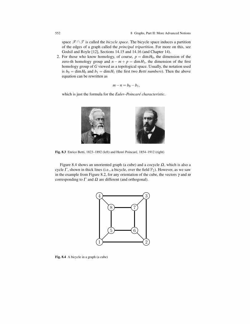
552 8 Graphs, Part II: More Advanced Notions
space F ∩T is called the bicycle space. The bicycle space induces a partitionof the edges of a graph called the principal tripartition. For more on this, seeGodsil and Royle [12], Sections 14.15 and 14.16 (and Chapter 14).
2. For those who know homology, of course, p = dimH0, the dimension of thezero-th homology group and n−m + p = dimH1, the dimension of the firsthomology group of G viewed as a topological space. Usually, the notation usedis b0 = dimH0 and b1 = dimH1 (the first two Betti numbers). Then the aboveequation can be rewritten as
m−n = b0−b1,
which is just the formula for the Euler–Poincare characteristic.
Fig. 8.3 Enrico Betti, 1823–1892 (left) and Henri Poincare, 1854–1912 (right)
Figure 8.4 shows an unoriented graph (a cube) and a cocycle Ω , which is also acycle Γ , shown in thick lines (i.e., a bicycle, over the field F2). However, as we sawin the example from Figure 8.2, for any orientation of the cube, the vectors γ and ω
corresponding to Γ and Ω are different (and orthogonal).
1
1 2
34
5 6
78
Fig. 8.4 A bicycle in a graph (a cube)

8.1 Γ -Cycles, Cocycles, Cotrees, Flows, and Tensions 553
Let us illustrate the procedures for constructing bases of F and T on the graphG8. Figure 8.5 shows a spanning tree T and a cotree K for G8.
We have n= 7;m= 5; p= 1, and so, dimF = 7−5+1= 3 and dimT = 5−1=4. If we successively add the edges e2, e6, and e7 to the spanning tree T , we get thethree simple cycles shown in Figure 8.6 with thicker lines.
If we successively add the edges e1, e3, e4, and e5 to the cotree K, we get the foursimple cocycles shown in Figures 8.7 and 8.8 with thicker lines.
Given any node v ∈ V in a graph G for simplicity of notation let us denotethe cocycle Ω(v) by Ω(v). Similarly, we write Ω+(v) for Ω+(v); Ω−(v) forΩ−(v), and similarly for the the vectors ω(v), and so on. It turns our thatvectors of the form ω(v) generate the cocycle space and this has important conse-quences.
Proposition 8.8. Given any finite directed graph G = (V,E,s, t) for every cocycleΩ = Ω(Y ) we have
ω(Y ) = ∑v∈Y
ω(v).
Consequently, the vectors of the form ω(v), with v ∈V , generate the cocycle spaceT .
Proof . For any edge e ∈ E if a = s(e) and b = t(e), observe that
ω(v)e =
+1 if v = a−1 if v = b0 if v 6= a,b.
As a consequence, if we evaluate ∑v∈Y ω(v), we find that(∑v∈Y
ω(v)
)e
=
+1 if a ∈ Y and b ∈V −Y−1 if a ∈V −Y and b ∈ Y0 if a,b ∈ Y or a,b ∈V −Y ,
which is exactly ω(Y )v. ut
1
v4
v5
v1 v2
v3
e1
e7
e2 e3 e4
e5
e6
G8 :
v4
v5
v1 v2
v3
e1
e3 e4
e5
T :
v4
v5
v1 v2
v3e7
e2
e6
K :
Fig. 8.5 Graph G8; A spanning tree, T ; a cotree, K
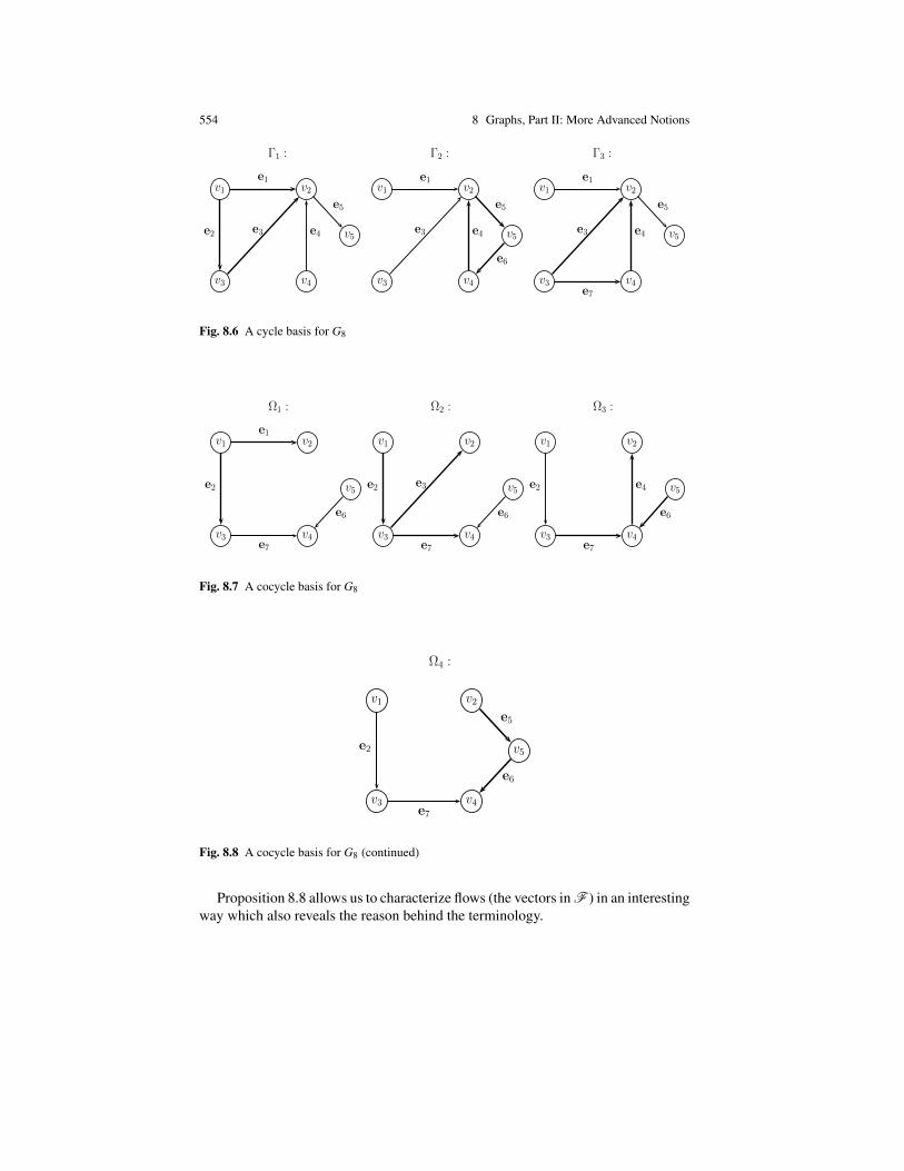
554 8 Graphs, Part II: More Advanced Notions
1
v4
v5
v1 v2
v3
e1
e2 e3 e4
e5
!1 :
v4
v5
v1 v2
v3
e1
e3 e4
e5
e6
!2 :
v4
v5
v1 v2
v3
e1
e7
e3 e4
e5
!3 :
Fig. 8.6 A cycle basis for G8
1
v4
v5
v1 v2
v3
e1
e7
e2
e6
!1 :
v4
v5
v1 v2
v3e7
e2 e3
e6
!2 :
v4
v5
v1 v2
v3e7
e2 e4
e6
!3 :
Fig. 8.7 A cocycle basis for G8
1
v4
v5
v1 v2
v3e7
e2
e5
e6
!4 :
Fig. 8.8 A cocycle basis for G8 (continued)
Proposition 8.8 allows us to characterize flows (the vectors in F ) in an interestingway which also reveals the reason behind the terminology.
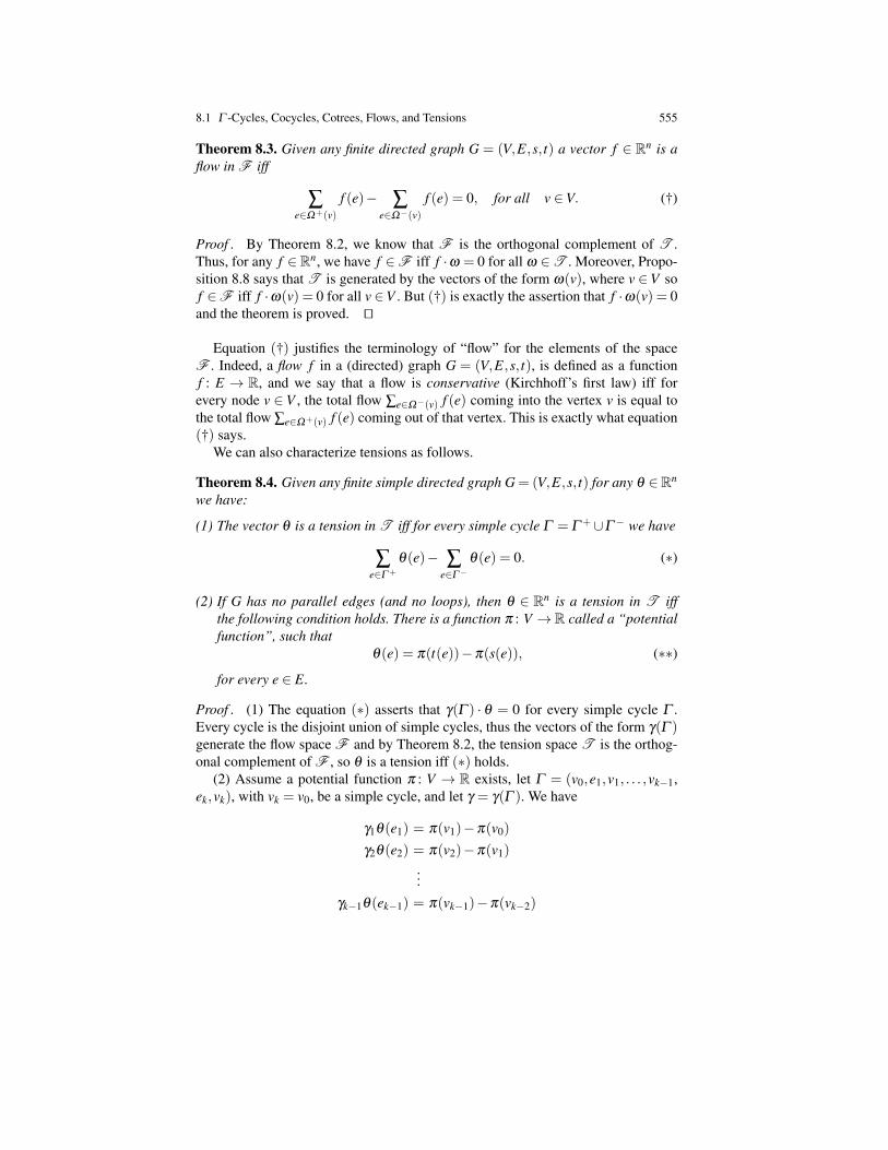
8.1 Γ -Cycles, Cocycles, Cotrees, Flows, and Tensions 555
Theorem 8.3. Given any finite directed graph G = (V,E,s, t) a vector f ∈ Rn is aflow in F iff
∑e∈Ω+(v)
f (e)− ∑e∈Ω−(v)
f (e) = 0, for all v ∈V. (†)
Proof . By Theorem 8.2, we know that F is the orthogonal complement of T .Thus, for any f ∈Rn, we have f ∈F iff f ·ω = 0 for all ω ∈T . Moreover, Propo-sition 8.8 says that T is generated by the vectors of the form ω(v), where v ∈V sof ∈F iff f ·ω(v) = 0 for all v ∈V . But (†) is exactly the assertion that f ·ω(v) = 0and the theorem is proved. ut
Equation (†) justifies the terminology of “flow” for the elements of the spaceF . Indeed, a flow f in a (directed) graph G = (V,E,s, t), is defined as a functionf : E → R, and we say that a flow is conservative (Kirchhoff’s first law) iff forevery node v ∈ V , the total flow ∑e∈Ω−(v) f (e) coming into the vertex v is equal tothe total flow ∑e∈Ω+(v) f (e) coming out of that vertex. This is exactly what equation(†) says.
We can also characterize tensions as follows.
Theorem 8.4. Given any finite simple directed graph G = (V,E,s, t) for any θ ∈Rn
we have:
(1) The vector θ is a tension in T iff for every simple cycle Γ = Γ +∪Γ− we have
∑e∈Γ+
θ(e)− ∑e∈Γ−
θ(e) = 0. (∗)
(2) If G has no parallel edges (and no loops), then θ ∈ Rn is a tension in T iffthe following condition holds. There is a function π : V →R called a “potentialfunction”, such that
θ(e) = π(t(e))−π(s(e)), (∗∗)for every e ∈ E.
Proof . (1) The equation (∗) asserts that γ(Γ ) · θ = 0 for every simple cycle Γ .Every cycle is the disjoint union of simple cycles, thus the vectors of the form γ(Γ )generate the flow space F and by Theorem 8.2, the tension space T is the orthog-onal complement of F , so θ is a tension iff (∗) holds.
(2) Assume a potential function π : V → R exists, let Γ = (v0,e1,v1, . . . ,vk−1,ek,vk), with vk = v0, be a simple cycle, and let γ = γ(Γ ). We have
γ1θ(e1) = π(v1)−π(v0)
γ2θ(e2) = π(v2)−π(v1)
...γk−1θ(ek−1) = π(vk−1)−π(vk−2)
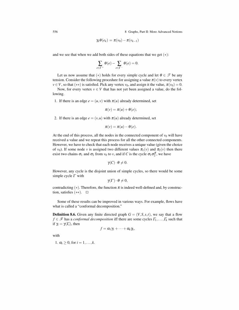
556 8 Graphs, Part II: More Advanced Notions
γkθ(ek) = π(v0)−π(vk−1)
and we see that when we add both sides of these equations that we get (∗):
∑e∈Γ+
θ(e)− ∑e∈Γ−
θ(e) = 0.
Let us now assume that (∗) holds for every simple cycle and let θ ∈ T be anytension. Consider the following procedure for assigning a value π(v) to every vertexv∈V , so that (∗∗) is satisfied. Pick any vertex v0, and assign it the value, π(v0) = 0.
Now, for every vertex v ∈ V that has not yet been assigned a value, do the fol-lowing.
1. If there is an edge e = (u,v) with π(u) already determined, set
π(v) = π(u)+θ(e);
2. If there is an edge e = (v,u) with π(u) already determined, set
π(v) = π(u)−θ(e).
At the end of this process, all the nodes in the connected component of v0 will havereceived a value and we repeat this process for all the other connected components.However, we have to check that each node receives a unique value (given the choiceof v0). If some node v is assigned two different values π1(v) and π2(v) then thereexist two chains σ1 and σ2 from v0 to v, and if C is the cycle σ1σR
2 , we have
γ(C) ·θ 6= 0.
However, any cycle is the disjoint union of simple cycles, so there would be somesimple cycle Γ with
γ(Γ ) ·θ 6= 0,
contradicting (∗). Therefore, the function π is indeed well-defined and, by construc-tion, satisfies (∗∗). ut
Some of these results can be improved in various ways. For example, flows havewhat is called a “conformal decomposition.”
Definition 8.6. Given any finite directed graph G = (V,S,s, t), we say that a flowf ∈F has a conformal decomposition iff there are some cycles Γ1, . . . ,Γk such thatif γi = γ(Γi), then
f = α1γ1 + · · ·+αkγk,
with
1. αi ≥ 0, for i = 1, . . . ,k.
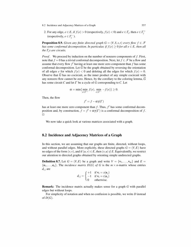
8.2 Incidence and Adjacency Matrices of a Graph 557
2. For any edge, e∈ E, if f (e)> 0 (respectively, f (e)< 0) and e∈Γj, then e∈Γ+j
(respectively, e ∈ Γ−j ).
Proposition 8.9. Given any finite directed graph G = (V,S,s, t) every flow f ∈Fhas some conformal decomposition. In particular, if f (e)≥ 0 for all e ∈ E, then allthe Γjs are circuits.
Proof . We proceed by induction on the number of nonzero components of f . First,note that f = 0 has a trivial conformal decomposition. Next, let f ∈F be a flow andassume that every flow f ′ having at least one more zero component than f has someconformal decomposition. Let G be the graph obtained by reversing the orientationof all edges e for which f (e) < 0 and deleting all the edges for which f (e) = 0.Observe that G has no cocircuit, as the inner product of any simple cocircuit withany nonzero flow cannot be zero. Hence, by the corollary to the coloring lemma, Ghas some circuit C and let Γ be a cycle of G corresponding to C. Let
α = minmine∈Γ+
f (e), mine∈Γ−
− f (e) ≥ 0.
Then, the flowf ′ = f −αγ(Γ )
has at least one more zero component than f . Thus, f ′ has some conformal decom-position and, by construction, f = f ′+αγ(Γ ) is a conformal decomposition of f .ut
We now take a quick look at various matrices associated with a graph.
8.2 Incidence and Adjacency Matrices of a Graph
In this section, we are assuming that our graphs are finite, directed, without loops,and without parallel edges. More explicitly, these directed graphs G = (V,E) haveno edges of the form (v,v), and if (u,v)∈E, then (v,u) /∈E. Equivalentlly, we restrictour attention to directed graphs obtained by orienting simple undirected graphs.
Definition 8.7. Let G = (V,E) be a graph and write V = v1, . . . ,vm and E =e1, . . . ,en. The incidence matrix D(G) of G is the m× n-matrix whose entriesdi j are
di j =
+1 if vi = s(e j)−1 if vi = t(e j)0 otherwise.
Remark: The incidence matrix actually makes sense for a graph G with paralleledges but without loops.
For simplicity of notation and when no confusion is possible, we write D insteadof D(G).
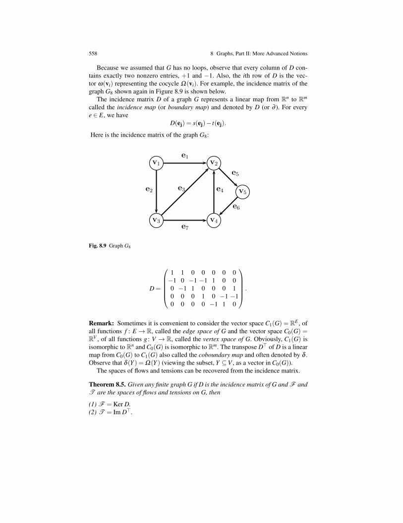
558 8 Graphs, Part II: More Advanced Notions
Because we assumed that G has no loops, observe that every column of D con-tains exactly two nonzero entries, +1 and −1. Also, the ith row of D is the vec-tor ω(vi) representing the cocycle Ω(vi). For example, the incidence matrix of thegraph G8 shown again in Figure 8.9 is shown below.
The incidence matrix D of a graph G represents a linear map from Rn to Rm
called the incidence map (or boundary map) and denoted by D (or ∂ ). For everye ∈ E, we have
D(ej) = s(ej)− t(ej).
Here is the incidence matrix of the graph G8:
1
v4
v5
v1 v2
v3
e1
e7
e2 e3 e4
e5
e6
Fig. 8.9 Graph G8
D =
1 1 0 0 0 0 0−1 0 −1 −1 1 0 00 −1 1 0 0 0 10 0 0 1 0 −1 −10 0 0 0 −1 1 0
.
Remark: Sometimes it is convenient to consider the vector space C1(G) = RE , ofall functions f : E → R, called the edge space of G and the vector space C0(G) =RV , of all functions g : V → R, called the vertex space of G. Obviously, C1(G) isisomorphic to Rn and C0(G) is isomorphic to Rm. The transpose D> of D is a linearmap from C0(G) to C1(G) also called the coboundary map and often denoted by δ .Observe that δ (Y ) = Ω(Y ) (viewing the subset, Y ⊆V , as a vector in C0(G)).
The spaces of flows and tensions can be recovered from the incidence matrix.
Theorem 8.5. Given any finite graph G if D is the incidence matrix of G and F andT are the spaces of flows and tensions on G, then
(1) F = Ker D.(2) T = Im D>.
8.2 Incidence and Adjacency Matrices of a Graph 559
Futhermore, if G has p connected components and m nodes, then
rankD = m− p.
Proof . We already observed that the ith row of D is the vector ω(vi) and we knowfrom Theorem 8.3 that F is exactly the set of vectors orthogonal to all vectors ofthe form ω(vi). Now, for any f ∈ Rn,
D f =
ω(v1) · f...
ω(vm) · f
,
and so, F =Ker D. The vectors ω(vi) generate T , therefore the rows of D generateT ; that is, T = Im D>.
From Theorem 8.2, we know that
dimT = m− p
and inasmuch as we just proved that T = Im D>, we get
rankD = rankD> = m− p,
which proves the last part of our theorem. ut
Corollary 8.3. For any graph G = (V,E,s, t) if |V | = m, |E| = n and G has p con-nected components, then the incidence matrix D of G has rank n (i.e., the columnsof D are linearly independent) iff F = (0) iff n = m− p.
Proof . By Theorem 8.3, we have rankD = m− p. So, rankD = n iff n = m− p iffn−m+ p = 0 iff F = (0) (because dimF = n−m+ p). ut
The incidence matrix of a graph has another interesting property observed byPoincare. First, let us define a variant of triangular matrices.
Definition 8.8. An n× n (real or complex) matrix A = (ai j) is said to be pseudo-triangular and nonsingular iff either
(i) n = 1 and a11 6= 0.(ii) n≥ 2 and A has some row, say k, with a unique nonzero entry ahk such that the
submatrix B obtained by deleting the hth row and the kth column from A is alsopseudo-triangular and nonsingular.
It is easy to see that a matrix defined as in Definition 8.8 can be transformed intoa usual triangular matrix by permutation of its columns.
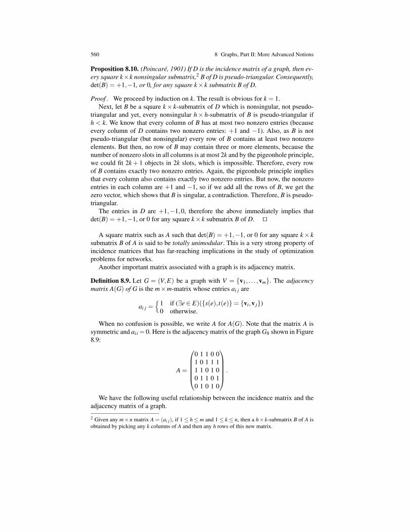
560 8 Graphs, Part II: More Advanced Notions
Proposition 8.10. (Poincare, 1901) If D is the incidence matrix of a graph, then ev-ery square k×k nonsingular submatrix,2 B of D is pseudo-triangular. Consequently,det(B) = +1,−1, or 0, for any square k× k submatrix B of D.
Proof . We proceed by induction on k. The result is obvious for k = 1.Next, let B be a square k× k-submatrix of D which is nonsingular, not pseudo-
triangular and yet, every nonsingular h× h-submatrix of B is pseudo-triangular ifh < k. We know that every column of B has at most two nonzero entries (becauseevery column of D contains two nonzero entries: +1 and −1). Also, as B is notpseudo-triangular (but nonsingular) every row of B contains at least two nonzeroelements. But then, no row of B may contain three or more elements, because thenumber of nonzero slots in all columns is at most 2k and by the pigeonhole principle,we could fit 2k+ 1 objects in 2k slots, which is impossible. Therefore, every rowof B contains exactly two nonzero entries. Again, the pigeonhole principle impliesthat every column also contains exactly two nonzero entries. But now, the nonzeroentries in each column are +1 and −1, so if we add all the rows of B, we get thezero vector, which shows that B is singular, a contradiction. Therefore, B is pseudo-triangular.
The entries in D are +1,−1,0, therefore the above immediately implies thatdet(B) = +1,−1, or 0 for any square k× k submatrix B of D. ut
A square matrix such as A such that det(B) = +1,−1, or 0 for any square k× ksubmatrix B of A is said to be totally unimodular. This is a very strong property ofincidence matrices that has far-reaching implications in the study of optimizationproblems for networks.
Another important matrix associated with a graph is its adjacency matrix.
Definition 8.9. Let G = (V,E) be a graph with V = v1, . . . ,vm. The adjacencymatrix A(G) of G is the m×m-matrix whose entries ai j are
ai j =
1 if (∃e ∈ E)(s(e), t(e)= vi,v j)0 otherwise.
When no confusion is possible, we write A for A(G). Note that the matrix A issymmetric and ai i = 0. Here is the adjacency matrix of the graph G8 shown in Figure8.9:
A =
0 1 1 0 01 0 1 1 11 1 0 1 00 1 1 0 10 1 0 1 0
.
We have the following useful relationship between the incidence matrix and theadjacency matrix of a graph.
2 Given any m×n matrix A = (ai j), if 1≤ h≤ m and 1≤ k ≤ n, then a h× k-submatrix B of A isobtained by picking any k columns of A and then any h rows of this new matrix.
8.2 Incidence and Adjacency Matrices of a Graph 561
Proposition 8.11. Given any graph G, if D is the incidence matrix of G, A is theadjacency matrix of G, and ∆ is the diagonal matrix such that ∆i i = d(vi), thedegree of node vi, then
DD> = ∆ −A.
Consequently, DD> is independent of the orientation of the underlying undirectedgraph of G, and ∆ −A is symmetric positive, semidefinite; that is, the eigenvaluesof ∆ −A are real and nonnegative.
Proof . It is well known that DD>i j is the inner product of the ith row di, and the jthrow d j of D. If i = j, then as
di k =
+1 if s(ek) = vi−1 if t(ek) = vi0 otherwise
we see that di · di = d(vi). If i 6= j, then di · d j 6= 0 iff there is some edge ek withs(ek) = vi and t(ek) = v j or vice-versa (which are mutually exclusive cases, byhypothesis on our graphs), in which case, di ·d j =−1. Therefore,
DD> = ∆ −A,
as claimed. Now, DD> is obviously symmetric and it is well known that its eigen-values are nonnegative (e.g., see Gallier [11], Chapter 12). ut
Remarks:
1. The matrix L = DD> = ∆ −A, is known as the Laplacian (matrix) of the graph,G. Another common notation for the matrix DD> is Q. The columns of D con-tain exactly the two nonzero entries, +1 and −1, thus we see that the vector 1,defined such that 1i = 1, is an eigenvector for the eigenvalue 0.
2. If G is connected, then D has rank m−1, so the rank of DD> is also m−1 andthe other eigenvalues of DD> besides 0 are strictly positive. The smallest pos-itive eigenvalue of L = DD> has some remarkable properties. There is an areaof graph theory overlapping (linear) algebra, called spectral graph theory thatinvestigates the properties of graphs in terms of the eigenvalues of its Laplacianmatrix but this is beyond the scope of this book. Some good references for al-gebraic graph theory include Biggs [3], Godsil and Royle [12], and Chung [6]for spectral graph theory.One of the classical and surprising results in algebraic graph theory is a formulathat gives the number of spanning trees τ(G) of a connected graph G in termsof its Laplacian L = DD>. If J denotes the square matrix whose entries are all1s and if adjL denotes the adjoint matrix of L (the transpose of the matrix ofcofactors of L), that is, the matrix given by
(adjL)i j = (−1)i+ j detL( j, i),

562 8 Graphs, Part II: More Advanced Notions
where L( j, i) is the matrix obtained by deleting the jth row and the ith columnof L, then we have
adjL = τ(G)J.
We also haveτ(G) = m−2 det(J+L),
where m is the number of nodes of G.3. As we already observed, the incidence matrix also makes sense for graphs with
parallel edges and no loops. But now, in order for the equation DD> = ∆ −A tohold, we need to define A differently. We still have the same definition as beforefor the incidence matrix but we can define the new matrix A such that
Ai j = |e ∈ E | s(e), t(e)= vi,v j|;
that is, Ai j is the total number of edges between vi and v j and between v j andvi. Then, we can check that
DD> = ∆ −A .
4. There are also versions of the adjacency matrix and of the incidence matrix forundirected graphs. In this case, D is no longer totally unimodular.
8.3 Eulerian and Hamiltonian Cycles
In this short section, we discuss two classical problems that go back to the verybeginning of graph theory. These problems have to do with the existence of certainkinds of cycles in graphs. These problems come in two flavors depending on whetherthe graphs are directed but there are only minor differences between the two versionsand traditionally the focus is on undirected graphs.
The first problem goes back to Euler and is usually known as the Konigsbergbridge problem. In 1736, the town of Konigsberg had seven bridges joining fourareas of land. Euler was asked whether it were possible to find a cycle that crossedevery bridge exactly once (and returned to the starting point).
The graph shown in Figure 8.11 models the Konigsberg bridge problem. Thenodes A,B,C,D correspond to four areas of land in Konigsberg and the edges to theseven bridges joining these areas of land.
In fact, the problem is unsolvable, as shown by Euler, because some nodes donot have an even degree. We now define the problem precisely and give a completesolution.
Definition 8.10. Given a finite undirected graph G = (V,E) (respectively, a directedgraph G = (V,E,s, t)) a Euler cycle (or Euler tour), (respectively, a Euler circuit) isa cycle in G that passes through every node and every edge (exactly once); (respec-tively, a circuit in G that passes through every node and every edge (exactly once)).

8.3 Eulerian and Hamiltonian Cycles 563
Fig. 8.10 Leonhard Euler, 1707–1783
1
B
A
C
D
Fig. 8.11 The seven bridges of Konigsberg and a graph modeling the Konigsberg bridge problem
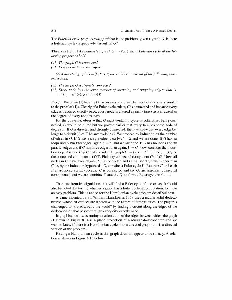
564 8 Graphs, Part II: More Advanced Notions
The Eulerian cycle (resp. circuit) problem is the problem: given a graph G, is therea Eulerian cycle (respectively, circuit) in G?
Theorem 8.6. (1) An undirected graph G = (V,E) has a Eulerian cycle iff the fol-lowing properties hold.
(a1) The graph G is connected.(b1) Every node has even degree.
(2) A directed graph G = (V,E,s, t) has a Eulerian circuit iff the following prop-erties hold.
(a2) The graph G is strongly connected.(b2) Every node has the same number of incoming and outgoing edges; that is,
d+(v) = d−(v), for all v ∈V.
Proof . We prove (1) leaving (2) as an easy exercise (the proof of (2) is very similarto the proof of (1)). Clearly, if a Euler cycle exists, G is connected and because everyedge is traversed exactly once, every node is entered as many times as it is exited sothe degree of every node is even.
For the converse, observe that G must contain a cycle as otherwise, being con-nected, G would be a tree but we proved earlier that every tree has some node ofdegree 1. (If G is directed and strongly connected, then we know that every edge be-longs to a circuit.) Let Γ be any cycle in G. We proceed by induction on the numberof edges in G. If G has a single edge, clearly Γ = G and we are done. If G has noloops and G has two edges, again Γ = G and we are done. If G has no loops and noparallel edges and if G has three edges, then again, Γ = G. Now, consider the induc-tion step. Assume Γ 6= G and consider the graph G′ = (V,E−Γ ). Let G1, . . . ,Gp bethe connected components of G′. Pick any connected component Gi of G′. Now, allnodes in Gi have even degree, Gi is connected and Gi has strictly fewer edges thanG so, by the induction hypothesis, Gi contains a Euler cycle Γi. But then Γ and eachΓi share some vertex (because G is connected and the Gi are maximal connectedcomponents) and we can combine Γ and the Γis to form a Euler cycle in G. ut
There are iterative algorithms that will find a Euler cycle if one exists. It shouldalso be noted that testing whether a graph has a Euler cycle is computationally quitean easy problem. This is not so for the Hamiltonian cycle problem described next.
A game invented by Sir William Hamilton in 1859 uses a regular solid dodeca-hedron whose 20 vertices are labeled with the names of famous cities. The player ischallenged to “travel around the world” by finding a circuit along the edges of thedodecahedron that passes through every city exactly once.
In graphical terms, assuming an orientation of the edges between cities, the graphD shown in Figure 8.14 is a plane projection of a regular dodecahedron and wewant to know if there is a Hamiltonian cycle in this directed graph (this is a directedversion of the problem).
Finding a Hamiltonian cycle in this graph does not appear to be so easy. A solu-tion is shown in Figure 8.15 below.

8.3 Eulerian and Hamiltonian Cycles 565
Fig. 8.12 William Hamilton, 1805–1865
Fig. 8.13 A Voyage Round the World Game and Icosian Game (Hamilton)
1
Fig. 8.14 A tour “around the world”
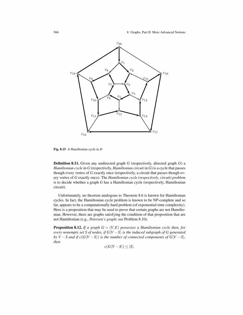
566 8 Graphs, Part II: More Advanced Notions
1
v18v17
v11v12 v13
v10v6
v5
v4
v14
v19
v9
v8
v7 v3
v2
v15
v16
v1
v20
Fig. 8.15 A Hamiltonian cycle in D
Definition 8.11. Given any undirected graph G (respectively, directed graph G) aHamiltonian cycle in G (respectively, Hamiltonian circuit in G) is a cycle that passesthough every vertex of G exactly once (respectively, a circuit that passes though ev-ery vertex of G exactly once). The Hamiltonian cycle (respectively, circuit) problemis to decide whether a graph G has a Hamiltonian cycle (respectively, Hamiltoniancircuit).
Unfortunately, no theorem analogous to Theorem 8.6 is known for Hamiltoniancycles. In fact, the Hamiltonian cycle problem is known to be NP-complete and sofar, appears to be a computationally hard problem (of exponential time complexity).Here is a proposition that may be used to prove that certain graphs are not Hamilto-nian. However, there are graphs satisfying the condition of that proposition that arenot Hamiltonian (e.g., Petersen’s graph; see Problem 8.10).
Proposition 8.12. If a graph G = (V,E) possesses a Hamiltonian cycle then, forevery nonempty set S of nodes, if G〈V −S〉 is the induced subgraph of G generatedby V − S and if c(G〈V − S〉) is the number of connected components of G〈V − S〉,then
c(G〈V −S〉)≤ |S|.
8.4 Network Flow Problems; The Max-Flow Min-Cut Theorem 567
Proof . Let Γ be a Hamiltonian cycle in G and let G be the graph G = (V,Γ ). If wedelete k vertices we can’t cut a cycle into more than k pieces and so
c(G〈V −S〉)≤ |S|.
However, we also have
c(G〈V −S〉)≤ c(G〈V −S〉),
which proves the proposition. ut
8.4 Network Flow Problems; The Max-Flow Min-Cut Theorem
The network flow problem is a perfect example of a problem that is important prac-tically but also theoretically because in both cases it has unexpected applications. Inthis section, we solve the network flow problem using some of the notions from Sec-tion 8.1. First, let us describe the kinds of graphs that we are dealing with, usuallycalled networks (or transportation networks or flow networks).
Definition 8.12. A network (or flow network) is a quadruple N = (G,c,vs,st), whereG is a finite digraph G = (V,E,s, t) without loops, c : E → R+ is a function calleda capacity function assigning a capacity c(e) > 0 (or cost or weight) to every edgee ∈ E, and vs,vt ∈ V are two (distinct) distinguished nodes.3 Moreover, we assumethat there are no edges coming into vs (d−G (vs) = 0), which is called the source andthat there are no outgoing edges from vt (d+
G (vt) = 0), which is called the terminal(or sink).
An example of a network is shown in Figure 8.16 with the capacity of each edgewithin parentheses.
Intuitively, we can think of the edges of a network as conduits for fluid, or wiresfor electricity, or highways for vehicle, and so on, and the capacity of each edge isthe maximum amount of “flow” that can pass through that edge. The purpose of anetwork is to carry “flow”, defined as follows.
Definition 8.13. Given a network N = (G,c,vs,vt) a flow in N is a function f : E→R such that the following conditions hold.
(1) (Conservation of flow)
∑t(e)=v
f (e) = ∑s(e)=v
f (e), for all v ∈V −vs,vt
3 Most books use the notation s and t for vs and vt . Sorry, s and t are already used in the definitionof a digraph.
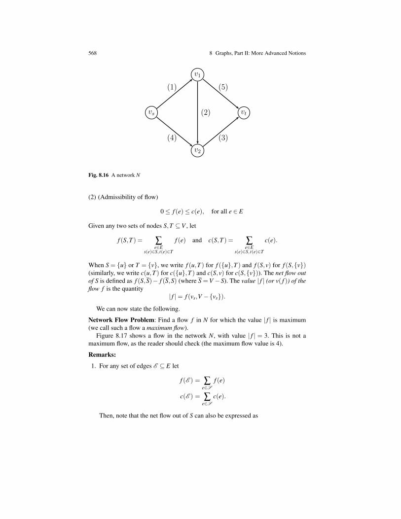
568 8 Graphs, Part II: More Advanced Notions
1
vs
v1
v2
vt
(1)
(4)
(5)
(3)
(2)
Fig. 8.16 A network N
(2) (Admissibility of flow)
0≤ f (e)≤ c(e), for all e ∈ E
Given any two sets of nodes S,T ⊆V , let
f (S,T ) = ∑e∈E
s(e)∈S, t(e)∈T
f (e) and c(S,T ) = ∑e∈E
s(e)∈S, t(e)∈T
c(e).
When S = u or T = v, we write f (u,T ) for f (u,T ) and f (S,v) for f (S,v)(similarly, we write c(u,T ) for c(u,T ) and c(S,v) for c(S,v)). The net flow outof S is defined as f (S,S)− f (S,S) (where S =V −S). The value | f | (or v( f )) of theflow f is the quantity
| f |= f (vs,V −vs).We can now state the following.
Network Flow Problem: Find a flow f in N for which the value | f | is maximum(we call such a flow a maximum flow).
Figure 8.17 shows a flow in the network N, with value | f | = 3. This is not amaximum flow, as the reader should check (the maximum flow value is 4).
Remarks:
1. For any set of edges E ⊆ E let
f (E ) = ∑e∈S
f (e)
c(E ) = ∑e∈S
c(e).
Then, note that the net flow out of S can also be expressed as
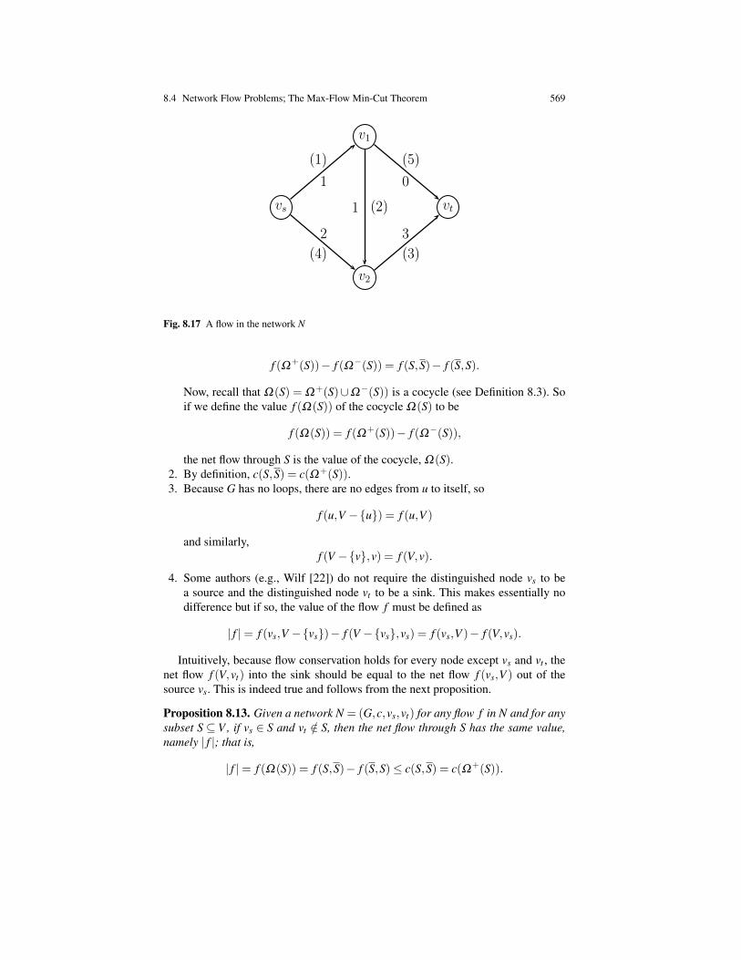
8.4 Network Flow Problems; The Max-Flow Min-Cut Theorem 569
1
vs
v1
v2
vt
(1)
(4)
(5)
(3)
(2)
1
2
0
3
1
Fig. 8.17 A flow in the network N
f (Ω+(S))− f (Ω−(S)) = f (S,S)− f (S,S).
Now, recall that Ω(S) = Ω+(S)∪Ω−(S)) is a cocycle (see Definition 8.3). Soif we define the value f (Ω(S)) of the cocycle Ω(S) to be
f (Ω(S)) = f (Ω+(S))− f (Ω−(S)),
the net flow through S is the value of the cocycle, Ω(S).2. By definition, c(S,S) = c(Ω+(S)).3. Because G has no loops, there are no edges from u to itself, so
f (u,V −u) = f (u,V )
and similarly,f (V −v,v) = f (V,v).
4. Some authors (e.g., Wilf [22]) do not require the distinguished node vs to bea source and the distinguished node vt to be a sink. This makes essentially nodifference but if so, the value of the flow f must be defined as
| f |= f (vs,V −vs)− f (V −vs,vs) = f (vs,V )− f (V,vs).
Intuitively, because flow conservation holds for every node except vs and vt , thenet flow f (V,vt) into the sink should be equal to the net flow f (vs,V ) out of thesource vs. This is indeed true and follows from the next proposition.
Proposition 8.13. Given a network N = (G,c,vs,vt) for any flow f in N and for anysubset S ⊆ V , if vs ∈ S and vt /∈ S, then the net flow through S has the same value,namely | f |; that is,
| f |= f (Ω(S)) = f (S,S)− f (S,S)≤ c(S,S) = c(Ω+(S)).

570 8 Graphs, Part II: More Advanced Notions
In particular,| f |= f (vs,V ) = f (V,vt).
Proof . Recall that | f |= f (vs,V ). Now, for any node v ∈ S−vs, because v 6= vt ,the equation
∑t(e)=v
f (e) = ∑s(e)=v
f (e)
holds and we see that
| f | = f (vs,V ) = ∑v∈S
( ∑s(e)=v
f (e)− ∑t(e)=v
f (e))
= ∑v∈S
( f (v,V )− f (V,v)) = f (S,V )− f (V,S).
However, V = S∪S, so
| f | = f (S,V )− f (V,S)
= f (S,S∪S)− f (S∪S,S)
= f (S,S)+ f (S,S)− f (S,S)− f (S,S)
= f (S,S)− f (S,S),
as claimed. The capacity of every edge is nonnegative, thus it is obvious that
| f |= f (S,S)− f (S,S)≤ f (S,S)≤ c(S,S) = c(Ω+(S)),
inasmuch as a flow is admissible. Finally, if we set S =V −vt, we get
f (S,S)− f (S,S) = f (V,vt)
and so, | f |= f (vs,V ) = f (V,vt). ut
Proposition 8.13 shows that the sets of edges Ω+(S) with vs ∈ S and vt /∈ S, playa very special role. Indeed, as a corollary of Proposition 8.13, we see that the valueof any flow in N is bounded by the capacity c(Ω+(S)) of the set Ω+(S) for any Swith vs ∈ S and vt /∈ S. This suggests the following definition.
Definition 8.14. Given a network N = (G,c,vs,vt), a cut separating vs and vt , forshort a vs-vt -cut, is any subset of edges C = Ω+(W ), where W is a subset of V withvs ∈W and vt /∈W . The capacity of a vs-vt -cut, C , is
c(C ) = c(Ω+(W )) = ∑e∈Ω+(W )
c(e).
Remark: Some authors, including Papadimitriou and Steiglitz [18] and Wilf [22],define a vs-vt -cut as a pair (W,W ), where W is a subset of V with with vs ∈W andvt /∈W . This definition is clearly equivalent to our definition above, which is due to

8.4 Network Flow Problems; The Max-Flow Min-Cut Theorem 571
Sakarovitch [21]. We have a slight prerefence for Definition 8.14 because it placesthe emphasis on edges as opposed to nodes. Indeed, the intuition behind vs-vt -cutsis that any flow from vs to vt must pass through some edge of any vs-vt -cut. Thus,it is not surprising that the capacity of vs-vt -cuts places a restriction on how muchflow can be sent from vs to vt .
We can rephrase Proposition 8.13 as follows.
Proposition 8.14. The maximum value of any flow f in the network N is boundedby the minimum capacity c(C ) of any vs-vt -cut C in N; that is,
max | f | ≤minc(C ).
Proposition 8.14 is half of the so-called max-flow min-cut theorem. The other halfof this theorem says that the above inequality is indeed an equality. That is, there isactually some vs-vt -cut C whose capacity c(C ) is the maximum value of the flowin N.
A vs-vt -cut of minimum capacity is called a minimum vs-vt -cut, for short, a min-imum cut.
An example of a minimum cut is shown in Figure 8.18, where
C = Ω+(vs,v2) = (vsv1),(v2vt),
these two edges being shown as thicker lines. The capacity of this cut is 4 and amaximum flow is also shown in Figure 8.18.
1
vs
v1
v2
vt
(1)
(4)
(5)
(3)
(2)
1
3
1
3
0
Fig. 8.18 A maximum flow and a minimum cut in the network N
What we intend to do next is to prove the celebrated “max-flow, min-cut theorem”(due to Ford and Fulkerson, 1957) and then to give an algorithm (also due to Fordand Fulkerson) for finding a maximum flow, provided some reasonable assumptionson the capacity function. In preparation for this, we present a handy trick (foundboth in Berge [1] and Sakarovitch [21]); the return edge.
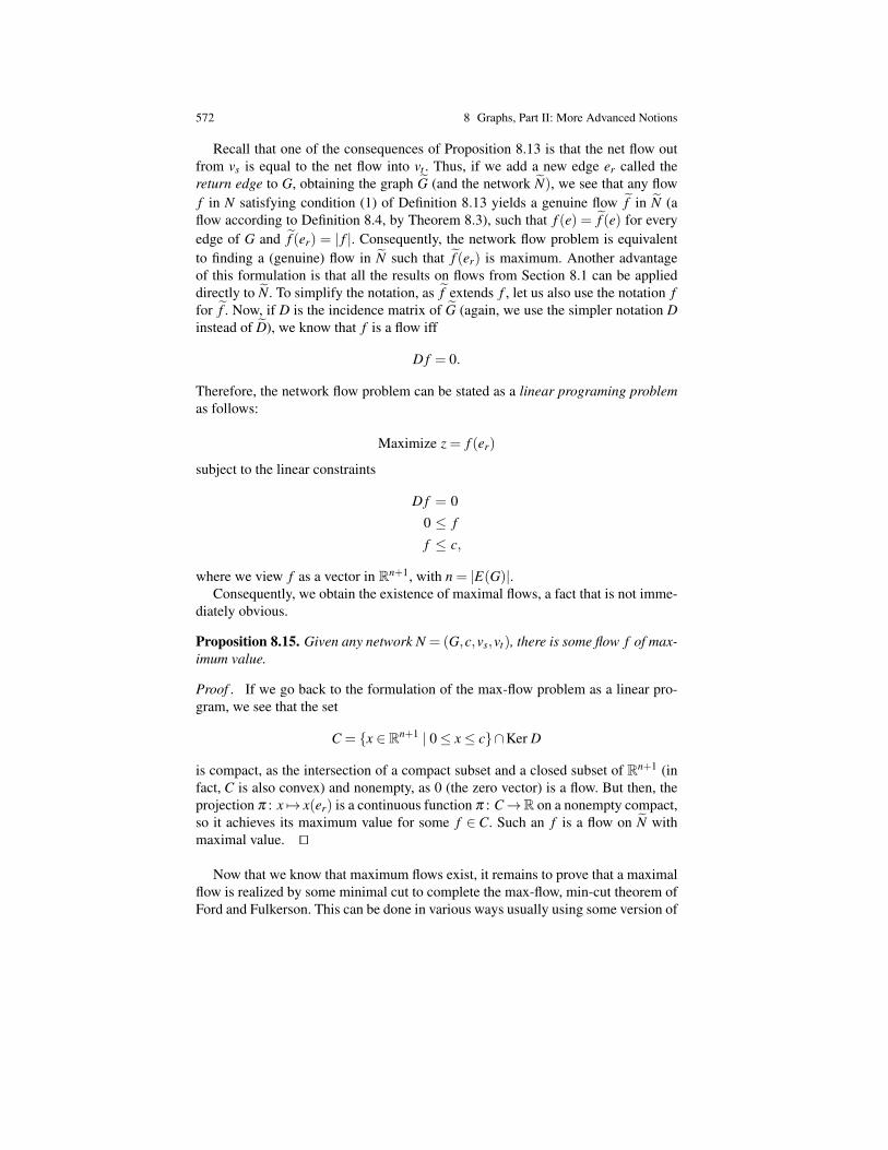
572 8 Graphs, Part II: More Advanced Notions
Recall that one of the consequences of Proposition 8.13 is that the net flow outfrom vs is equal to the net flow into vt . Thus, if we add a new edge er called thereturn edge to G, obtaining the graph G (and the network N), we see that any flowf in N satisfying condition (1) of Definition 8.13 yields a genuine flow f in N (aflow according to Definition 8.4, by Theorem 8.3), such that f (e) = f (e) for everyedge of G and f (er) = | f |. Consequently, the network flow problem is equivalentto finding a (genuine) flow in N such that f (er) is maximum. Another advantageof this formulation is that all the results on flows from Section 8.1 can be applieddirectly to N. To simplify the notation, as f extends f , let us also use the notation ffor f . Now, if D is the incidence matrix of G (again, we use the simpler notation Dinstead of D), we know that f is a flow iff
D f = 0.
Therefore, the network flow problem can be stated as a linear programing problemas follows:
Maximize z = f (er)
subject to the linear constraints
D f = 00 ≤ f
f ≤ c,
where we view f as a vector in Rn+1, with n = |E(G)|.Consequently, we obtain the existence of maximal flows, a fact that is not imme-
diately obvious.
Proposition 8.15. Given any network N = (G,c,vs,vt), there is some flow f of max-imum value.
Proof . If we go back to the formulation of the max-flow problem as a linear pro-gram, we see that the set
C = x ∈ Rn+1 | 0≤ x≤ c∩Ker D
is compact, as the intersection of a compact subset and a closed subset of Rn+1 (infact, C is also convex) and nonempty, as 0 (the zero vector) is a flow. But then, theprojection π : x 7→ x(er) is a continuous function π : C→R on a nonempty compact,so it achieves its maximum value for some f ∈ C. Such an f is a flow on N withmaximal value. ut
Now that we know that maximum flows exist, it remains to prove that a maximalflow is realized by some minimal cut to complete the max-flow, min-cut theorem ofFord and Fulkerson. This can be done in various ways usually using some version of

8.4 Network Flow Problems; The Max-Flow Min-Cut Theorem 573
an algorithm due to Ford and Fulkerson. Such proofs can be found in Papadimitriouand Steiglitz [18], Wilf [22], Cameron [5], and Sakarovitch [21].
Fig. 8.19 Delbert Ray Fulkerson, 1924–1976
Sakarovitch makes the interesting observation (given as an exercise) that the arccoloring lemma due to Minty (Theorem 8.1) yields a simple proof of the part of themax-flow, min-cut theorem that we seek to establish. (See [21], Chapter 4, Exercise1, page 105.) Therefore, we choose to present such a proof because it is ratheroriginal and quite elegant.
Theorem 8.7. (Max-Flow, Min-Cut Theorem (Ford and Fulkerson)) For any net-work N = (G,c,vs,vt), the maximum value | f | of any flow f in N is equal to theminimum capacity c(C ) of any vs-vt -cut C in N.
Proof . By Proposition 8.14, we already have half of our theorem. By Proposition8.15, we know that some maximum flow, say f , exists. It remains to show that thereis some vs-vt -cut C such that | f |= c(C ).
We proceed as follows.Form the graph G = (V,E ∪er,s, t) from G = (V,E,s, t), with s(er) = vt and
t(er)= vs. Then, form the graph, G=(V, E, s, t), whose edges are defined as follows.
(a) er ∈ E; s(er) = s(er), t(er) = t(er).(b) If e ∈ E and 0 < f (e)< c(e), then e ∈ E; s(e) = s(e), t(e) = t(e).(c) If e ∈ E and f (e) = 0, then e ∈ E; s(e) = s(e), t(e) = t(e).(d) If e ∈ E and f (e) = c(e), then e ∈ E, with s(e) = t(e) and t(e) = s(e).
In order to apply Minty’s theorem, we color all edges constructed in (a), (c), and(d) in black and all edges constructed in (b) in red and we pick er as the distinguishededge. Now, apply Minty’s lemma. We have two possibilities:
1. There is a simple cycle Γ in G, with all black edges oriented the same way.Because er is coming into vs, the direction of the cycle is from vs to vt , soer ∈ Γ +. This implies that all edges of type (d), e ∈ E, have an orientationconsistent with the direction of the cycle. Now, Γ is also a cycle in G and, inG, each edge e ∈ E with f (e) = c(e) is oriented in the inverse direction of thecycle; that is, e ∈ Γ− in G. Also, all edges of type (c), e ∈ E, with f (e) = 0, are
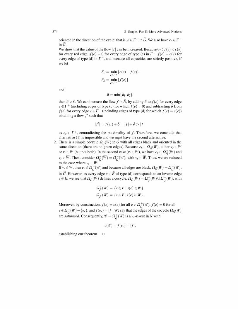
574 8 Graphs, Part II: More Advanced Notions
oriented in the direction of the cycle; that is, e∈Γ + in G. We also have er ∈Γ +
in G.We show that the value of the flow | f | can be increased. Because 0< f (e)< c(e)for every red edge, f (e) = 0 for every edge of type (c) in Γ +, f (e) = c(e) forevery edge of type (d) in Γ−, and because all capacities are strictly positive, ifwe let
δ1 = mine∈Γ+c(e)− f (e)
δ2 = mine∈Γ− f (e)
andδ = minδ1,δ2,
then δ > 0. We can increase the flow f in N, by adding δ to f (e) for every edgee ∈ Γ + (including edges of type (c) for which f (e) = 0) and subtracting δ fromf (e) for every edge e ∈ Γ− (including edges of type (d) for which f (e) = c(e))obtaining a flow f ′ such that
| f ′|= f (er)+δ = | f |+δ > | f |,
as er ∈ Γ +, contradicting the maximality of f . Therefore, we conclude thatalternative (1) is impossible and we must have the second alternative.
2. There is a simple cocycle ΩG(W ) in G with all edges black and oriented in thesame direction (there are no green edges). Because er ∈ ΩG(W ), either vs ∈Wor vt ∈W (but not both). In the second case (vt ∈W ), we have er ∈Ω
+
G(W ) and
vs ∈W . Then, consider Ω+
G(W ) = Ω
−G(W ), with vs ∈W . Thus, we are reduced
to the case where vs ∈W .If vs ∈W , then er ∈Ω
−G(W ) and because all edges are black, ΩG(W ) =Ω
−G(W ),
in G. However, as every edge e ∈ E of type (d) corresponds to an inverse edgee ∈ E, we see that ΩG(W ) defines a cocycle, ΩG(W ) = Ω
+
G(W )∪Ω
−G(W ), with
Ω+
G(W ) = e ∈ E | s(e) ∈W
Ω−G(W ) = e ∈ E | t(e) ∈W.
Moreover, by construction, f (e) = c(e) for all e ∈Ω+
G(W ), f (e) = 0 for all
e∈Ω−G(W )−er, and f (er)= | f |. We say that the edges of the cocycle ΩG(W )
are saturated. Consequently, C = Ω+
G(W ) is a vs-vt -cut in N with
c(C ) = f (er) = | f |,
establishing our theorem. ut
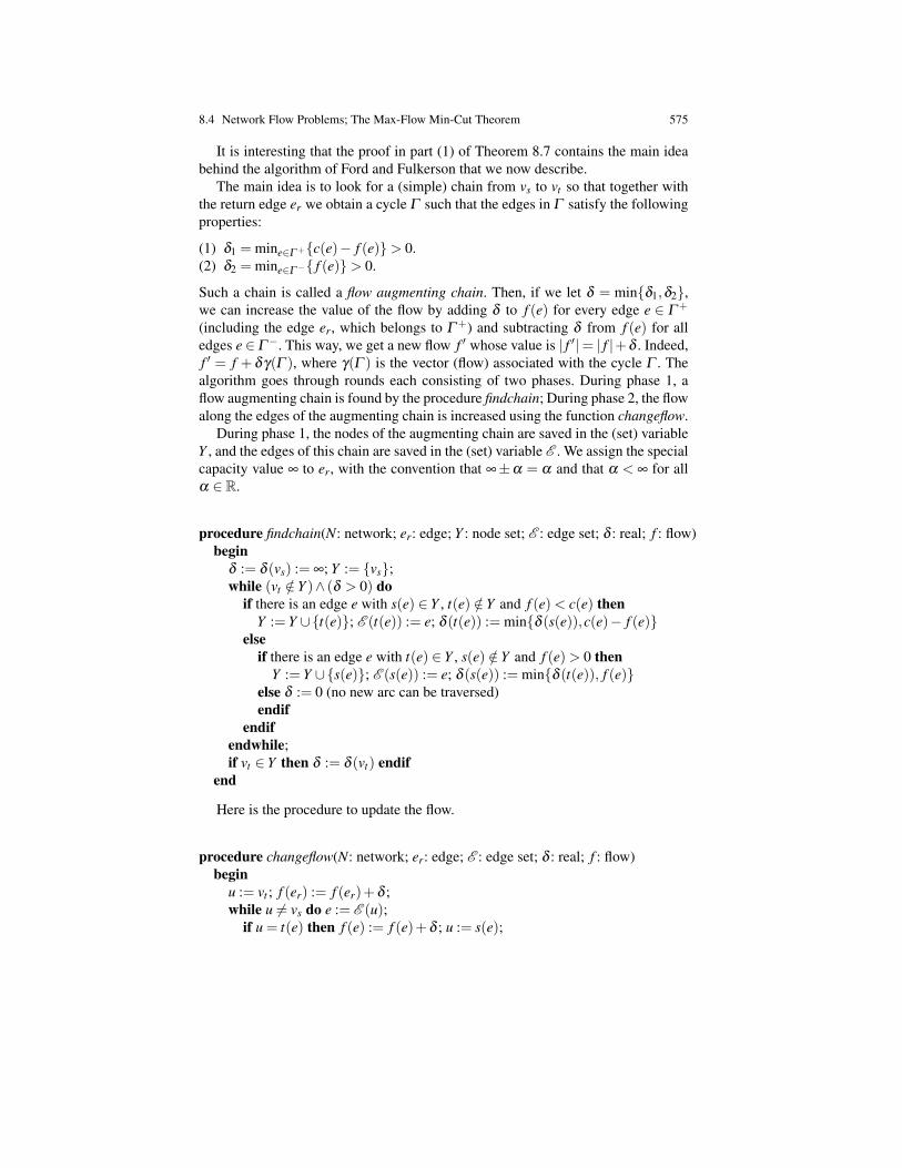
8.4 Network Flow Problems; The Max-Flow Min-Cut Theorem 575
It is interesting that the proof in part (1) of Theorem 8.7 contains the main ideabehind the algorithm of Ford and Fulkerson that we now describe.
The main idea is to look for a (simple) chain from vs to vt so that together withthe return edge er we obtain a cycle Γ such that the edges in Γ satisfy the followingproperties:
(1) δ1 = mine∈Γ+c(e)− f (e)> 0.(2) δ2 = mine∈Γ− f (e)> 0.
Such a chain is called a flow augmenting chain. Then, if we let δ = minδ1,δ2,we can increase the value of the flow by adding δ to f (e) for every edge e ∈ Γ +
(including the edge er, which belongs to Γ +) and subtracting δ from f (e) for alledges e ∈ Γ−. This way, we get a new flow f ′ whose value is | f ′|= | f |+δ . Indeed,f ′ = f + δγ(Γ ), where γ(Γ ) is the vector (flow) associated with the cycle Γ . Thealgorithm goes through rounds each consisting of two phases. During phase 1, aflow augmenting chain is found by the procedure findchain; During phase 2, the flowalong the edges of the augmenting chain is increased using the function changeflow.
During phase 1, the nodes of the augmenting chain are saved in the (set) variableY , and the edges of this chain are saved in the (set) variable E . We assign the specialcapacity value ∞ to er, with the convention that ∞±α = α and that α < ∞ for allα ∈ R.
procedure findchain(N: network; er: edge; Y : node set; E : edge set; δ : real; f : flow)begin
δ := δ (vs) := ∞; Y := vs;while (vt /∈ Y )∧ (δ > 0) do
if there is an edge e with s(e) ∈ Y , t(e) /∈ Y and f (e)< c(e) thenY := Y ∪t(e); E (t(e)) := e; δ (t(e)) := minδ (s(e)),c(e)− f (e)
elseif there is an edge e with t(e) ∈ Y , s(e) /∈ Y and f (e)> 0 then
Y := Y ∪s(e); E (s(e)) := e; δ (s(e)) := minδ (t(e)), f (e)else δ := 0 (no new arc can be traversed)endif
endifendwhile;if vt ∈ Y then δ := δ (vt) endif
end
Here is the procedure to update the flow.
procedure changeflow(N: network; er: edge; E : edge set; δ : real; f : flow)begin
u := vt ; f (er) := f (er)+δ ;while u 6= vs do e := E (u);
if u = t(e) then f (e) := f (e)+δ ; u := s(e);
576 8 Graphs, Part II: More Advanced Notions
else f (e) := f (e)−δ ; u = t(e)endif
endwhileend
Finally, the algorithm maxflow is given below.
procedure maxflow(N: network; er: edge; Y : set of nodes; E : set of edges; f : flow)begin
for each e ∈ E do f (e) := 0 enfdor;repeat until δ = 0
findchain(N,er,Y,E ,δ , f );if δ > 0 then
changeflow(N,er,E ,δ , f )endif
endrepeatend
The reader should run the algorithm maxflow on the network of Figure 8.16to verify that the maximum flow shown in Figure 8.18 is indeed found, withY = vs,v2 when the algorithm stops.
The correctness of the algorithm maxflow is easy to prove.
Theorem 8.8. If the algorithm maxflow terminates and during the last round throughfindchain the node vt is not marked, then the flow f returned by the algorithm is amaximum flow.
Proof . Observe that if Y is the set of nodes returned when maxflow halts, thenvs ∈ Y , vt /∈ Y , and
1. If e ∈ Ω+(Y ), then f (e) = c(e), as otherwise, procedure findchain would haveadded t(e) to Y .
2. If e ∈ Ω−(Y ), then f (e) = 0, as otherwise, procedure findchain would haveadded s(e) to Y .
But then, as in the end of the proof of Theorem 8.7, we see that the edges of thecocycle Ω(Y ) are saturated and we know that Ω+(Y ) is a minimal cut and that| f |= c(Ω+(Y )) is maximal. ut
We still have to show that the algorithm terminates but there is a catch. Indeed,the version of the Ford and Fulkerson algorithm that we just presented may notterminate if the capacities are irrational. Moreover, in the limit, the flow found bythe algorithm may not be maximum. An example of this bad behavior due to Fordand Fulkerson is reproduced in Wilf [22] (Chapter 3, Section 5). However, we canprove the following termination result which, for all practical purposes, is goodenough, because only rational numbers can be stored by a computer.
8.4 Network Flow Problems; The Max-Flow Min-Cut Theorem 577
Theorem 8.9. Given a network N if all the capacities are multiples of some num-ber λ then the algorithm, maxflow, always terminates. In particular, the algorithmmaxflow always terminates if the capacities are rational (or integral).
Proof . The number δ will always be a multiple of λ , so f (er) will increase by atleast λ during each iteration. Thus, eventually, the value of a minimal cut, which isa multiple of λ , will be reached. ut
If all the capacities are integers, an easy induction yields the following useful andnontrivial proposition.
Proposition 8.16. Given a network N if all the capacities are integers, then the al-gorithm maxflow outputs a maximum flow f : E → N such that the flow in everyedge is an integer.
Remark: Proposition 8.16 only asserts that some maximum flow is of the formf : E → N. In general, there is more than one maximum flow and other maximumflows may not have integer values on all edges.
Theorem 8.9 is good news but it is also bad news from the point of view ofcomplexity. Indeed, the present version of the Ford and Fulkerson algorithm has arunning time that depends on capacities and so, it can be very bad.
There are various ways of getting around this difficulty to find algorithms thatdo not depend on capacities and quite a few researchers have studied this problem.An excellent discussion of the progress in network flow algorithms can be found inWilf [22] (Chapter 3).
A fairly simple modification of the Ford and Fulkerson algorithm consists inlooking for flow augmenting chains of shortest length. To explain this algorithm weneed the concept of residual network, which is a useful tool in any case. Given a net-work N = (G,c,s, t) and given any flow f , the residual network N f = (G f ,c f ,v f ,vt)is defined as follows.
1. Vf =V .2. For every edge, e∈ E, if f (e)< c(e), then e+ ∈ E f , s f (e+) = s(e), t f (e+) = t(e)
and c f (e+) = c(e)− f (e); the edge e+ is called a forward edge.3. For every edge, e ∈ E, if f (e) > 0, then e− ∈ E f , s f (e−) = t(e), t f (e−) = s(e)
and c f (e−) = f (e); the edge e− is called a backward edge because it has theinverse orientation of the original edge, e ∈ E.
The capacity c f (eε) of an edge eε ∈E f (with ε =±) is usually called the residualcapacity of eε . Observe that the same edge e in G, will give rise to two edges e+
and e− (with the same set of endpoints but with opposite orientations) in G f if0 < f (e) < c(e). Thus, G f has at most twice as many edges as G. Also, note thatevery edge e ∈ E which is saturated (i.e., for which f (e) = c(e)), does not survivein G f .
Observe that there is a one-to-one correspondence between (simple) flow aug-menting chains in the original graph G and (simple) flow augmenting paths in G f .

578 8 Graphs, Part II: More Advanced Notions
Furthermore, in order to check that a simple path π from vs to vt in G f is a flowaugmenting path, all we have to do is to compute
c f (π) = mineε∈πc f (eε),
the bottleneck of the path π . Then, as before, we can update the flow f in N to getthe new flow f ′ by setting
f ′(e) = f (e)+ c f (π), if e+ ∈ π
f ′(e) = f (e)− c f (π) if e− ∈ π,
f ′(e) = f (e) if e ∈ E and eε /∈ π,
for every edge e ∈ E. Note that the function fπ : E→ R, defined by
fπ(e) = c f (π), if e+ ∈ π
fπ(e) =−c f (π) if e− ∈ π,
fπ(e) = 0 if e ∈ E and eε /∈ π,
is a flow in N with | fπ |= c f (π) and f ′= f + fπ is a flow in N, with | f ′|= | f |+c f (π)(same reasoning as before). Now, we can repeat this process. Compute the newresidual graph N f ′ from N and f ′, update the flow f ′ to get the new flow f ′′ in N,and so on.
The same reasoning as before shows that if we obtain a residual graph with noflow augmenting path from vs to vt , then a maximum flow has been found.
It should be noted that a poor choice of augmenting paths may cause the algo-rithm to perform a lot more steps than necessary. For example, if we consider thenetwork shown in Figure 8.20, and if we pick the flow augmenting paths in theresidual graphs to be alternatively (vs,v1,v2,vt) and (vs,v2,v1,vt), at each step, weonly increase the flow by 1, so it will take 200 steps to find a maximum flow.
One of the main advantages of using residual graphs is that they make it con-venient to look for better strategies for picking flow augmenting paths. For exam-ple, we can choose a simple flow augmenting path of shortest length (e.g., usingbreadth-first search). Then, it can be shown that this revised algorithm terminatesin O(|V | · |E|) steps (see Cormen et al. [7], Section 26.2, and Sakarovitch [21],Chapter 4, Exercise 5). Edmonds and Karp designed an algorithm running in timeO(|E| · |V |2) based on this idea (1972), see [7], Section 26.2. Another way of se-lecting “good” augmenting paths, the scaling max-flow algorithm, is described inKleinberg and Tardos [16] (see Section 7.3).
Here is an illustration of this faster algorithm, starting with the network N shownin Figure 8.16. The sequence of residual network construction and flow augmenta-tion steps is shown in Figures 8.21–8.23. During the first two rounds, the augmentedpath chosen is shown in thicker lines. In the third and final round, there is no pathfrom vs to vt in the residual graph, indicating that a maximum flow has been found.
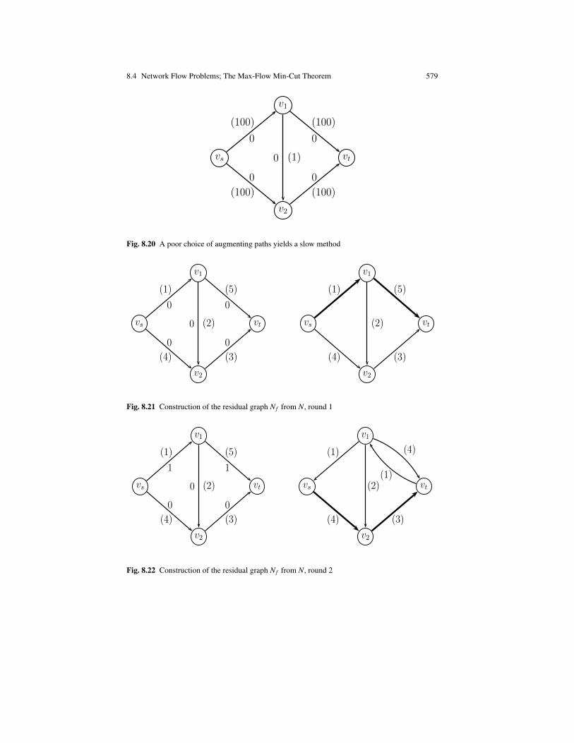
8.4 Network Flow Problems; The Max-Flow Min-Cut Theorem 579
1
vs
v1
v2
vt
(100)
(100)
(100)
(100)
(1)
0
0
0
0
0
Fig. 8.20 A poor choice of augmenting paths yields a slow method
1
vs
v1
v2
vt
(1)
(4)
(5)
(3)
(2)
0
0
0
0
0 vs
v1
v2
vt
(1)
(4)
(5)
(3)
(2)
Fig. 8.21 Construction of the residual graph N f from N, round 1
1
vs
v1
v2
vt
(1)
(4)
(5)
(3)
(2)
1
0
1
0
0 vs
v1
v2
vt
(1)
(4)
(4)
(1)
(3)
(2)
Fig. 8.22 Construction of the residual graph N f from N, round 2

580 8 Graphs, Part II: More Advanced Notions
1
vs
v1
v2
vt
(1)
(4)
(5)
(3)
(2)
1
3
1
3
0 vs
v1
v2
vt
(1)
(1)
(3)
(4)
(1)
(3)
(2)
Fig. 8.23 Construction of the residual graph N f from N, round 3
Another idea originally due to Dinic (1970) is to use layered networks; see Wilf[22] (Sections 3.6–3.7) and Papadimitriou and Steiglitz [18] (Chapter 9). An algo-rithm using layered networks running in time O(V 3) is given in the two referencesabove. There are yet other faster algorithms, for instance “preflow-push algorithms”also called “preflow-push relabel algorithms,” originally due to Goldberg. A preflowis a function f : E→ R that satisfies Condition (2) of Definition 8.13 but which, in-stead of satisfying Condition (1), satisfies the inequality
(1′) (Nonnegativity of net flow)
∑s(e)=v
f (e)≥ ∑t(e)=v
f (e) for all v ∈V −vs,vt;
that is, the net flow out of v is nonnegative. Now, the principle of all methods usingpreflows is to augment a preflow until it becomes a maximum flow. In order to dothis, a labeling algorithm assigning a height is used. Algorithms of this type arediscussed in Cormen et al. [7], Sections 26.4 and 26.5 and in Kleinberg and Tardos[16], Section 7.4.
The max-flow, min-cut theorem (Theorem 8.7) is a surprisingly powerful theo-rem in the sense that it can be used to prove a number of other results whose originalproof is sometimes quite hard. Among these results, let us mention the maximummatching problem in a bipartite graph, discussed in Wilf [22] (Sections 3.8), Cor-men et al. [7] (Section 26.3), Kleinberg and Tardos [16] (Section 7.5), and Cameron[5] (Chapter 11, Section 10), finding the edge connectivity of a graph, discussed inWilf [22] (Sections 3.8), and a beautiful theorem of Menger on edge-disjoint pathsand Hall’s Marriage Theorem, both discussed in Cameron [5] (Chapter 11, Section10). More problems that can be solved effectively using flow algorithms, includingimage segmentation, are discussed in Sections 7.6–7.13 of Kleinberg and Tardos[16]. We only mention one of Menger’s theorems, as it is particularly elegant.

8.4 Network Flow Problems; The Max-Flow Min-Cut Theorem 581
Fig. 8.24 Karl Menger, 1902–1985
Theorem 8.10. (Menger) Given any finite digraph G for any two nodes vs and vt ,the maximum number of pairwise edge-disjoint paths from vs to vt is equal to thethe minimum number of edges in a vs-vt -separating set. (A a vs-vt -separating set inG is a set of edges C such every path from vs to vt uses some edge in C.)
It is also possible to generalize the basic flow problem in which our flows f havethe property that 0 ≤ f (e) ≤ c(e) for every edge e ∈ E, to channeled flows. Thisgeneralization consists in adding another capacity function b : E → R, relaxing thecondition that c(e) > 0 for all e ∈ E, and in allowing flows such that condition (2)of Definition 8.13 is replaced by the following.
(2′) (Admissibility of flow)
b(e)≤ f (e)≤ c(e), for all e ∈ E
Now, the “flow” f = 0 is no longer necessarily admissible and the channeled flowproblem does not always have a solution. However, it is possible to characterizewhen it has a solution.
Theorem 8.11. (Hoffman) A network N = (G,b,c,vs,vt) has a channeled flow iff forevery cocycle Ω(Y ) of G we have
∑e∈Ω−(Y )
b(e)≤ ∑e∈Ω+(Y )
c(e). (†)
Observe that the necessity of the condition of Theorem 8.11 is an immediateconsequence of Proposition 8.5. That it is sufficient can be proved by modifyingthe algorithm maxflow or its version using residual networks. The principle of thismethod is to start with a flow f in N that does not necessarily satisfy Condition (2′)and to gradually convert it to an admissible flow in N (if one exists) by applyingthe method for finding a maximum flow to a modified version N of N in which thecapacities have been adjusted so that f is an admissible flow in N. Now, if a flowf in N does not satisfy Condition (2′), then there are some offending edges e forwhich either f (e) < b(e) or f (e) > c(e). The new method makes sure that at theend of every (successful) round through the basic maxflow algorithm applied to themodified network N some offending edge of N is no longer offending.
582 8 Graphs, Part II: More Advanced Notions
Let f be a flow in N and assume that e is an offending edge (i.e., eitherf (e) < b(e) or f (e) > c(e)). Then, we construct the network N( f , e) as follows.The capacity functions b and c are given by
b(e) =
b(e) if b(e)≤ f (e)f (e) if f (e)< b(e)
and
c(e) =
c(e) if f (e)≤ c(e)f (e) if f (e)> c(e).
We also add one new edge er to N whose endpoints and capacities are determinedby:
1. If f (e)> c(e), then s(er) = t(e), t(er) = s(e), b(er) = 0 and c(er) = f (e)−c(e).2. If f (e)< b(e), then s(er)= s(e), t(er)= t(e), b(er)= 0 and c(er)= b(e)− f (e).
Now, observe that the original flow f in N extended so that f (er) = 0 is a chan-neled flow in N( f , e) (i.e., Conditions (1) and (2′) are satisfied). Starting from thenew network N( f , e) apply the max-flow algorithm, say using residual graphs, withthe following small change in 2.
1. For every edge e∈ E, if f (e)< c(e), then e+ ∈ E f , s f (e+) = s(e), t f (e+) = t(e)and c f (e+) = c(e)− f (e); the edge e+ is called a forward edge.
2. For every edge e∈ E, if f (e)> b(e), then e− ∈ E f , s f (e−) = t(e), t f (e−) = s(e)and c f (e−) = f (e)− b(e); the edge e− is called a backward edge.
Now, we consider augmenting paths from t(er) to s(er). For any such simple pathπ in N( f , e) f , as before we compute
c f (π) = mineε∈πc f (eε),
the bottleneck of the path π , and we say that π is a flow augmenting path iff c f (π)>
0. Then, we can update the flow f in N( f , e) to get the new flow f ′ by setting
f ′(e) = f (e)+ c f (π) if e− ∈ π,
f ′(e) = f (e)− c f (π) if e− ∈ π,
f ′(e) = f (e) if e ∈ E and eε /∈ π,
for every edge e ∈ E.We run the flow augmenting path procedure on N( f , e) and f until it terminates
with a maximum flow f . If we recall that the offending edge is e, then there are fourcases:
1. f (e)> c(e).
a. When the max-flow algorithm terminates, f (er) = c(er) = f (e)− c(e). Ifso, define f as follows.
8.4 Network Flow Problems; The Max-Flow Min-Cut Theorem 583
f (e) =
f (e)− f (er) if e = ef (e) if e 6= e.
(∗)
It is clear that f is a flow in N and f (e) = c(e) (there are no simple pathsfrom t(e) to s(e)). But then, e is not an offending edge for f , so we repeatthe procedure of constructing the modified network, etc.
b. When the max-flow algorithm terminates, f (er) < c(er). The flow f de-fined in (∗) above, is still a flow but the max-flow algorithm must haveterminated with a residual graph with no flow augmenting path from s(e)to t(e). Then, there is a set of nodes Y with s(e)∈Y and t(e) /∈Y . Moreover,the way the max-flow algorithm is designed implies that
f (e)> c(e)
f (e) = c(e)≥ c(e) if e ∈Ω+(Y )−e
f (e) = b(e)≤ b(e) if e ∈Ω−(Y ).
As f also satisfies (∗) above, we conclude that the cocycle condition (†)of Theorem 8.11 fails for Ω(Y ).
2. f (e)< b(e).
a. When the max-flow algorithm terminates, f (er) = c(er) = b(e)− f (e). Ifso, define f as follows.
f (e) =
f (e)+ f (er) if e = ef (e) if e 6= e.
(∗∗)
It is clear that f is a flow in N and f (e) = b(e) (there are no simple pathsfrom s(e) to t(e)). But then, e is not an offending edge for f , so we repeatthe procedure of constructing the modified network, and so on.
b. When the max-flow algorithm terminates, f (er) < c(er). The flow f de-fined in (∗∗) above is still a flow but the max-flow algorithm must haveterminated with a residual graph with no flow augmenting path from t(e)to s(e). Then, as in the case where f (e) > c(e), there is a set of nodes Ywith s(e) ∈Y and t(e) /∈Y and it is easy to show that the cocycle condition(†) of Theorem 8.11 fails for Ω(Y ).
Therefore, if the algorithm does not fail during every round through the max-flowalgorithm applied to the modified network N, which, as we observed, is the case ifCondition (†) holds, then a channeled flow f will be produced and this flow will bea maximum flow. This proves the converse of Theorem 8.11.
The max-flow, min-cut theorem can also be generalized to channeled flows asfollows.
584 8 Graphs, Part II: More Advanced Notions
Theorem 8.12. For any network N = (G,b,c,vs,vt), if a flow exists in N, then themaximum value | f | of any flow f in N is equal to the minimum capacity c(Ω(Y )) =c(Ω+(Y ))−b(Ω−(Y )) of any vs-vt -cocycle in N (this means that vs ∈Y and vr /∈Y ).
If the capacity functions b and c have the property that b(e)< 0 and c(e)> 0 forall e ∈ E, then the condition of Theorem 8.11 is trivially satisfied. Furthermore, inthis case, the flow f = 0 is admissible, Proposition 8.15 holds, and we can applydirectly the construction of the residual network N f described above.
A variation of our last problem appears in Cormen et al. [7] (Chapter 26). In thisversion, the underlying graph G of the network N, is assumed to have no paralleledges (and no loops), so that every edge e can be identified with the pair (u,v) of itsendpoints (so, E ⊆ V ×V ). A flow f in N is a function f : V ×V → R, where it isnot necessarily the case that f (u,v)≥ 0 for all (u,v), but there is a capacity functionc : V ×V → R such that c(u,v)≥ 0, for all (u,v) ∈V ×V and it is required that
f (v,u) = − f (u,v) andf (u,v) ≤ c(u,v),
for all (u,v) ∈V ×V . Moreover, in view of the skew symmetry condition ( f (v,u) =− f (u,v)), the equations of conservation of flow are written as
∑(u,v)∈E
f (u,v) = 0,
for all u 6= vs,vt .We can reduce this last version of the flow problem to our previous setting by
noticing that in view of skew symmetry, the capacity conditions are equivalent tohaving capacity functions b′ and c′, defined such that
b′(u,v) = −c(v,u)
c′(u,v) = c(u,v),
for every (u,v) ∈ E and f must satisfy
b′(u,v)≤ f (u,v)≤ c′(u,v),
for all (u,v) ∈ E. However, we must also have f (v,u) = − f (u,v), which is an ad-ditional constraint in case G has both edges (u,v) and (v,u). This point may be alittle confusing because in our previous setting, f (u,v) and f (v,u) are independentvalues. However, this new problem is solved essentially as the previous one. Theconstruction of the residual graph is identical to the previous case and so is the flowaugmentation procedure along a simple path, except that we force fπ(v,u)= fπ(u,v)to hold during this step. For details, the reader is referred to Cormen et al. [7], Chap-ter 26.
More could be said about flow problems but we believe that we have covered thebasics satisfactorily and we refer the reader to the various references mentioned inthis section for more on this topic.
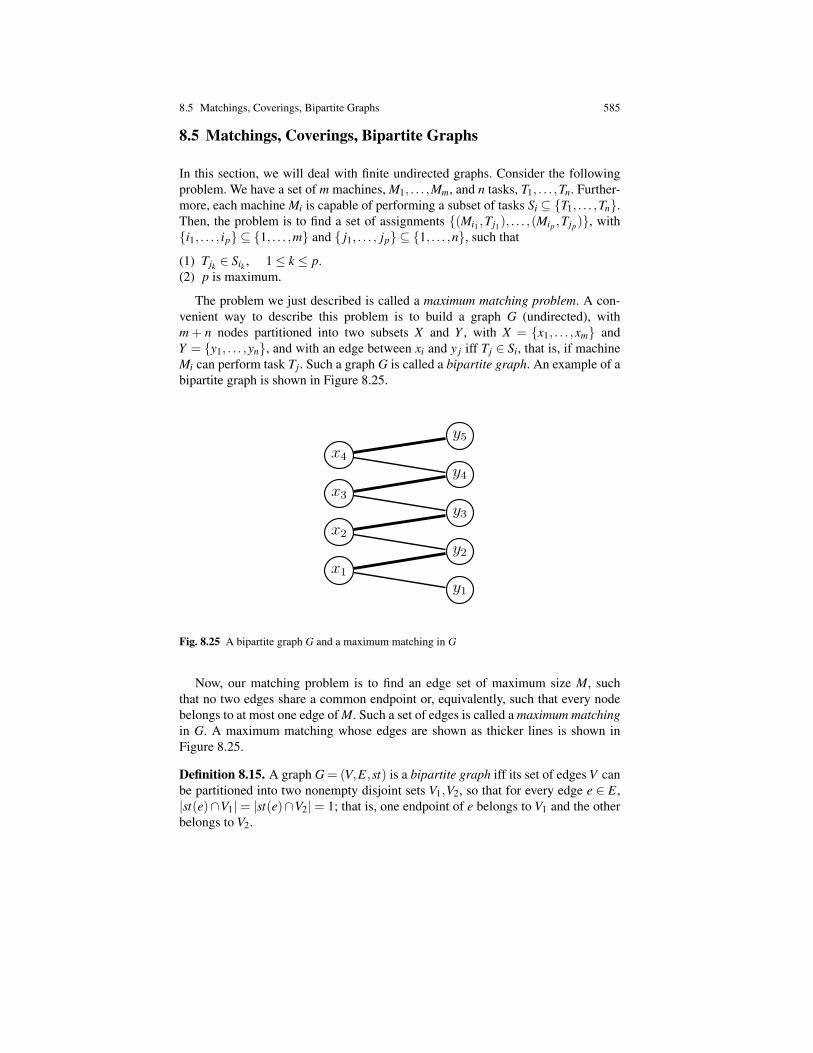
8.5 Matchings, Coverings, Bipartite Graphs 585
8.5 Matchings, Coverings, Bipartite Graphs
In this section, we will deal with finite undirected graphs. Consider the followingproblem. We have a set of m machines, M1, . . . ,Mm, and n tasks, T1, . . . ,Tn. Further-more, each machine Mi is capable of performing a subset of tasks Si ⊆ T1, . . . ,Tn.Then, the problem is to find a set of assignments (Mi1 ,Tj1), . . . ,(Mip ,Tjp), withi1, . . . , ip ⊆ 1, . . . ,m and j1, . . . , jp ⊆ 1, . . . ,n, such that
(1) Tjk ∈ Sik , 1≤ k ≤ p.(2) p is maximum.
The problem we just described is called a maximum matching problem. A con-venient way to describe this problem is to build a graph G (undirected), withm + n nodes partitioned into two subsets X and Y , with X = x1, . . . ,xm andY = y1, . . . ,yn, and with an edge between xi and y j iff Tj ∈ Si, that is, if machineMi can perform task Tj. Such a graph G is called a bipartite graph. An example of abipartite graph is shown in Figure 8.25.
1
x1
x2
x3
x4
y1
y2
y3
y4
y5
Fig. 8.25 A bipartite graph G and a maximum matching in G
Now, our matching problem is to find an edge set of maximum size M, suchthat no two edges share a common endpoint or, equivalently, such that every nodebelongs to at most one edge of M. Such a set of edges is called a maximum matchingin G. A maximum matching whose edges are shown as thicker lines is shown inFigure 8.25.
Definition 8.15. A graph G = (V,E,st) is a bipartite graph iff its set of edges V canbe partitioned into two nonempty disjoint sets V1,V2, so that for every edge e ∈ E,|st(e)∩V1|= |st(e)∩V2|= 1; that is, one endpoint of e belongs to V1 and the otherbelongs to V2.
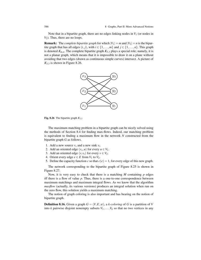
586 8 Graphs, Part II: More Advanced Notions
Note that in a bipartite graph, there are no edges linking nodes in V1 (or nodes inV2). Thus, there are no loops.
Remark: The complete bipartite graph for which |V1|=m and |V2|= n is the bipar-tite graph that has all edges (i, j), with i ∈ 1, . . . ,m and j ∈ 1, . . . ,n. This graphis denoted Km,n. The complete bipartite graph K3,3 plays a special role; namely, it isnot a planar graph, which means that it is impossible to draw it on a plane withoutavoiding that two edges (drawn as continuous simple curves) intersect. A picture ofK3,3 is shown in Figure 8.26.
1
x1
x2
x3
y1
y2
y3
Fig. 8.26 The bipartite graph K3,3
The maximum matching problem in a bipartite graph can be nicely solved usingthe methods of Section 8.4 for finding max-flows. Indeed, our matching problemis equivalent to finding a maximum flow in the network N constructed from thebipartite graph G as follows.
1. Add a new source vs and a new sink vt .2. Add an oriented edge (vs,u) for every u ∈V1.3. Add an oriented edge (v,vt) for every v ∈V2.4. Orient every edge e ∈ E from V1 to V2.5. Define the capacity function c so that c(e) = 1, for every edge of this new graph.
The network corresponding to the bipartite graph of Figure 8.25 is shown inFigure 8.27.
Now, it is very easy to check that there is a matching M containing p edgesiff there is a flow of value p. Thus, there is a one-to-one correspondence betweenmaximum matchings and maximum integral flows. As we know that the algorithmmaxflow (actually, its various versions) produces an integral solution when run onthe zero flow, this solution yields a maximum matching.
The notion of graph coloring is also important and has bearing on the notion ofbipartite graph.
Definition 8.16. Given a graph G = (V,E,st), a k-coloring of G is a partition of Vinto k pairwise disjoint nonempty subsets V1, . . . ,Vk so that no two vertices in any
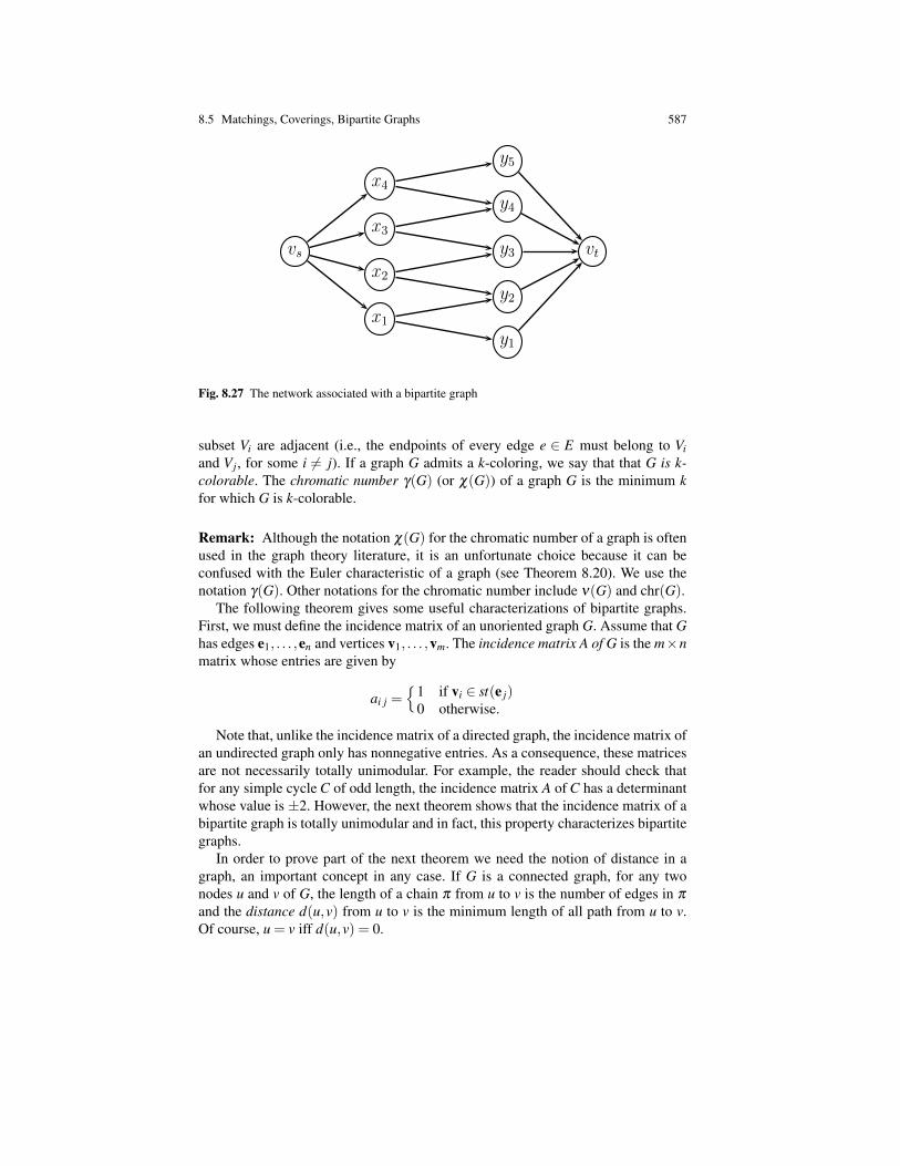
8.5 Matchings, Coverings, Bipartite Graphs 587
1
vs vt
x1
x2
x3
x4
y1
y2
y3
y4
y5
Fig. 8.27 The network associated with a bipartite graph
subset Vi are adjacent (i.e., the endpoints of every edge e ∈ E must belong to Viand Vj, for some i 6= j). If a graph G admits a k-coloring, we say that that G is k-colorable. The chromatic number γ(G) (or χ(G)) of a graph G is the minimum kfor which G is k-colorable.
Remark: Although the notation χ(G) for the chromatic number of a graph is oftenused in the graph theory literature, it is an unfortunate choice because it can beconfused with the Euler characteristic of a graph (see Theorem 8.20). We use thenotation γ(G). Other notations for the chromatic number include ν(G) and chr(G).
The following theorem gives some useful characterizations of bipartite graphs.First, we must define the incidence matrix of an unoriented graph G. Assume that Ghas edges e1, . . . ,en and vertices v1, . . . ,vm. The incidence matrix A of G is the m×nmatrix whose entries are given by
ai j =
1 if vi ∈ st(e j)0 otherwise.
Note that, unlike the incidence matrix of a directed graph, the incidence matrix ofan undirected graph only has nonnegative entries. As a consequence, these matricesare not necessarily totally unimodular. For example, the reader should check thatfor any simple cycle C of odd length, the incidence matrix A of C has a determinantwhose value is ±2. However, the next theorem shows that the incidence matrix of abipartite graph is totally unimodular and in fact, this property characterizes bipartitegraphs.
In order to prove part of the next theorem we need the notion of distance in agraph, an important concept in any case. If G is a connected graph, for any twonodes u and v of G, the length of a chain π from u to v is the number of edges in π
and the distance d(u,v) from u to v is the minimum length of all path from u to v.Of course, u = v iff d(u,v) = 0.
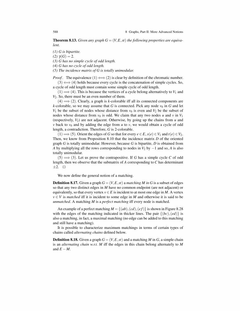
588 8 Graphs, Part II: More Advanced Notions
Theorem 8.13. Given any graph G = (V,E,st) the following properties are equiva-lent.
(1) G is bipartite.(2) γ(G) = 2.(3) G has no simple cycle of odd length.(4) G has no cycle of odd length.(5) The incidence matrix of G is totally unimodular.
Proof . The equivalence (1)⇐⇒ (2) is clear by definition of the chromatic number.(3)⇐⇒ (4) holds because every cycle is the concatenation of simple cycles. So,
a cycle of odd length must contain some simple cycle of odd length.(1) =⇒ (4). This is because the vertices of a cycle belong alternatively to V1 and
V2. So, there must be an even number of them.(4) =⇒ (2). Clearly, a graph is k-colorable iff all its connected components are
k-colorable, so we may assume that G is connected. Pick any node v0 in G and letV1 be the subset of nodes whose distance from v0 is even and V2 be the subset ofnodes whose distance from v0 is odd. We claim that any two nodes u and v in V1(respectively, V2) are not adjacent. Otherwise, by going up the chains from u andv back to v0 and by adding the edge from u to v, we would obtain a cycle of oddlength, a contradiction. Therefore, G is 2-colorable.
(1) =⇒ (5). Orient the edges of G so that for every e∈ E, s(e)∈V1 and t(e)∈V2.Then, we know from Proposition 8.10 that the incidence matrix D of the orientedgraph G is totally unimodular. However, because G is bipartite, D is obtained fromA by multiplying all the rows corresponding to nodes in V2 by −1 and so, A is alsototally unimodular.
(5) =⇒ (3). Let us prove the contrapositive. If G has a simple cycle C of oddlength, then we observe that the submatrix of A corresponding to C has determinant±2. ut
We now define the general notion of a matching.
Definition 8.17. Given a graph G = (V,E,st) a matching M in G is a subset of edgesso that any two distinct edges in M have no common endpoint (are not adjacent) orequivalently, so that every vertex v∈E is incident to at most one edge in M. A vertexv ∈ V is matched iff it is incident to some edge in M and otherwise it is said to beunmatched. A matching M is a perfect matching iff every node is matched.
An example of a perfect matching M = (ab),(cd),(e f ) is shown in Figure 8.28with the edges of the matching indicated in thicker lines. The pair (bc),(ed) isalso a matching, in fact, a maximal matching (no edge can be added to this matchingand still have a matching).
It is possible to characterize maximum matchings in terms of certain types ofchains called alternating chains defined below.
Definition 8.18. Given a graph G= (V,E,st) and a matching M in G, a simple chainis an alternating chain w.r.t. M iff the edges in this chain belong alternately to Mand E−M.
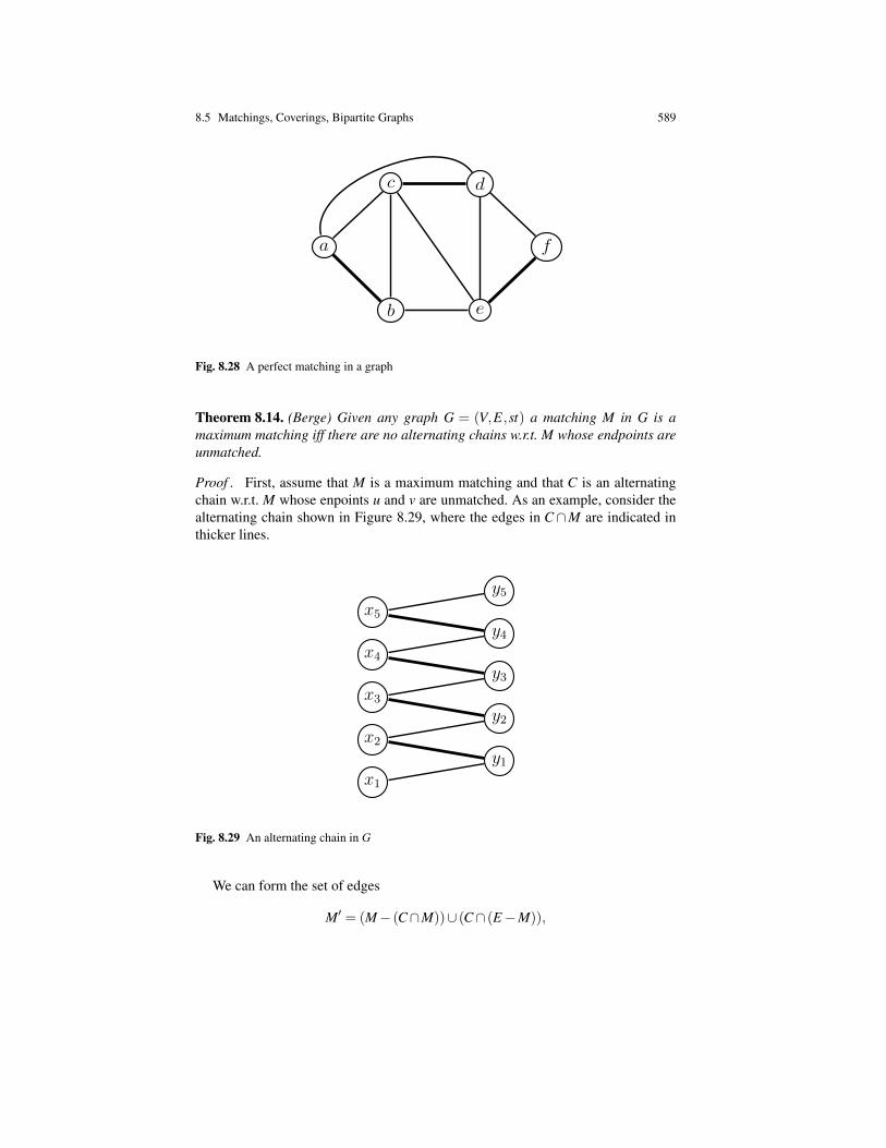
8.5 Matchings, Coverings, Bipartite Graphs 589
1
a
c
b
d
e
f
Fig. 8.28 A perfect matching in a graph
Theorem 8.14. (Berge) Given any graph G = (V,E,st) a matching M in G is amaximum matching iff there are no alternating chains w.r.t. M whose endpoints areunmatched.
Proof . First, assume that M is a maximum matching and that C is an alternatingchain w.r.t. M whose enpoints u and v are unmatched. As an example, consider thealternating chain shown in Figure 8.29, where the edges in C∩M are indicated inthicker lines.
1
x1
x2
x3
x4
x5
y1
y2
y3
y4
y5
Fig. 8.29 An alternating chain in G
We can form the set of edges
M′ = (M− (C∩M))∪ (C∩ (E−M)),
590 8 Graphs, Part II: More Advanced Notions
which consists in deleting the edges in M from C and adding the edges from C notin M. It is immediately verified that M′ is still a matching but |M′| = |M|+ 1 (seeFigure 8.29), contradicting the fact that M is a maximum matching. Therefore, thereare no alternating chains w.r.t. M whose endpoints are unmatched.
Conversely, assume that G has no alternating chains w.r.t. M whose endpointsare unmatched and let M′ be another matching with |M′| > |M| (i.e., M is not amaximum matching). Consider the spanning subgraph H of G, whose set of edgesis
(M−M′)∪ (M′−M).
As M and M′ are matchings, the connected components of H are either isolatedvertices, or simple cycles of even length, or simple chains, and in these last twocases, the edges in these cycles or chains belong alternately to M and M′; this isbecause dH(u)≤ 2 for every vertex u∈V and if dH(u) = 2, then u is adjacent to oneedge in M and one edge in M′.
Now, H must possess a connected component that is a chain C whose endpointsare in M′, as otherwise we would have |M′| ≤ |M|, contradicting the assumption|M′| > |M|. However, C is an alternating chain w.r.t. M whose endpoints are un-matched, a contradiction. ut
A notion closely related to the concept of a matching but, in some sense, dual, isthe notion of a line cover.
Definition 8.19. Given any graph G = (V,E,st) without loops or isolated vertices, aline cover (or line covering) of G is a set of edges C ⊆ E so that every vertex u ∈Vis incident to some edge in C . A minimum line cover C is a line cover of minimumsize.
The maximum matching M in the graph of Figure 8.28 is also a minimum linecover. The set (ab),(bc),(de),(e f ) is also a line cover but it is not minimum,although minimal. The relationship between maximum matchings and minimumline covers is given by the following theorem.
Theorem 8.15. Given any graph G = (V,E,st) without loops or isolated vertices,with |V | = n, let M be a maximum matching and let C be a minimum line cover.Then, the following properties hold.
(1) If we associate with every unmatched vertex of V some edge incident to thisvertex and add all such edges to M, then we obtain a minimum line cover, CM .
(2) Every maximum matching M′ of the spanning subgraph (V,C ) is a maximummatching of G.
(3) |M|+ |C |= n.
Proof . It is clear that CM is a line cover. As the number of vertices unmatched byM is n−2|M| (as each edge in M matches exactly two vertices), we have
|CM|= |M|+n−2|M|= n−|M|. (∗)

8.5 Matchings, Coverings, Bipartite Graphs 591
Furthermore, as C is a minimum line cover, the spanning subgraph (V,C ) does notcontain any cycle or chain of length greater than or equal to 2. Consequently, eachedge e ∈ C −M′ corresponds to a single vertex unmatched by M′. Thus,
|C |− |M′|= n−2|M′|;
that is,|C |= n−|M′|. (∗∗)
As M is a maximum matching of G,
|M′| ≤ |M|
and so, using (∗) and (∗∗), we get
|CM|= n−|M| ≤ n−|M′|= |C |;
that is, |CM| ≤ |C |. However, C is a minimum matching, so |C | ≤ |CM|, whichproves that
|C |= |CM|.The last equation proves the remaining claims. ut
There are also notions analogous to matchings and line covers but applying tovertices instead of edges.
Definition 8.20. Let G = (V,E,st) be any graph. A set U ⊆V of nodes is indepen-dent (or stable) iff no two nodes in U are adjacent (there is no edge having thesenodes as endpoints). A maximum independent set is an independent set of maximumsize. A set U ⊆V of nodes is a point cover (or vertex cover or transversal) iff everyedge of E is incident to some node in U . A minimum point cover is a point coverof minimum size.
For example, a,b,c,d, f is a point cover of the graph of Figure 8.28. The fol-lowing simple proposition holds.
Proposition 8.17. Let G = (V,E,st) be any graph, U be any independent set, C beany line cover, U be any point cover, and M be any matching. Then, we have thefollowing inequalities.
(1) |U | ≤ |C |.(2) |M| ≤ |U |.(3) U is an independent set of nodes iff V −U is a point cover.
Proof . (1) Because U is an independent set of nodes, every edge in C is incidentwith at most one vertex in U , so |U | ≤ |C |.
(2) Because M is a matching, every vertex in U is incident to at most one edgein M, so |M| ≤ |U |.
(3) Clear from the definitions. ut
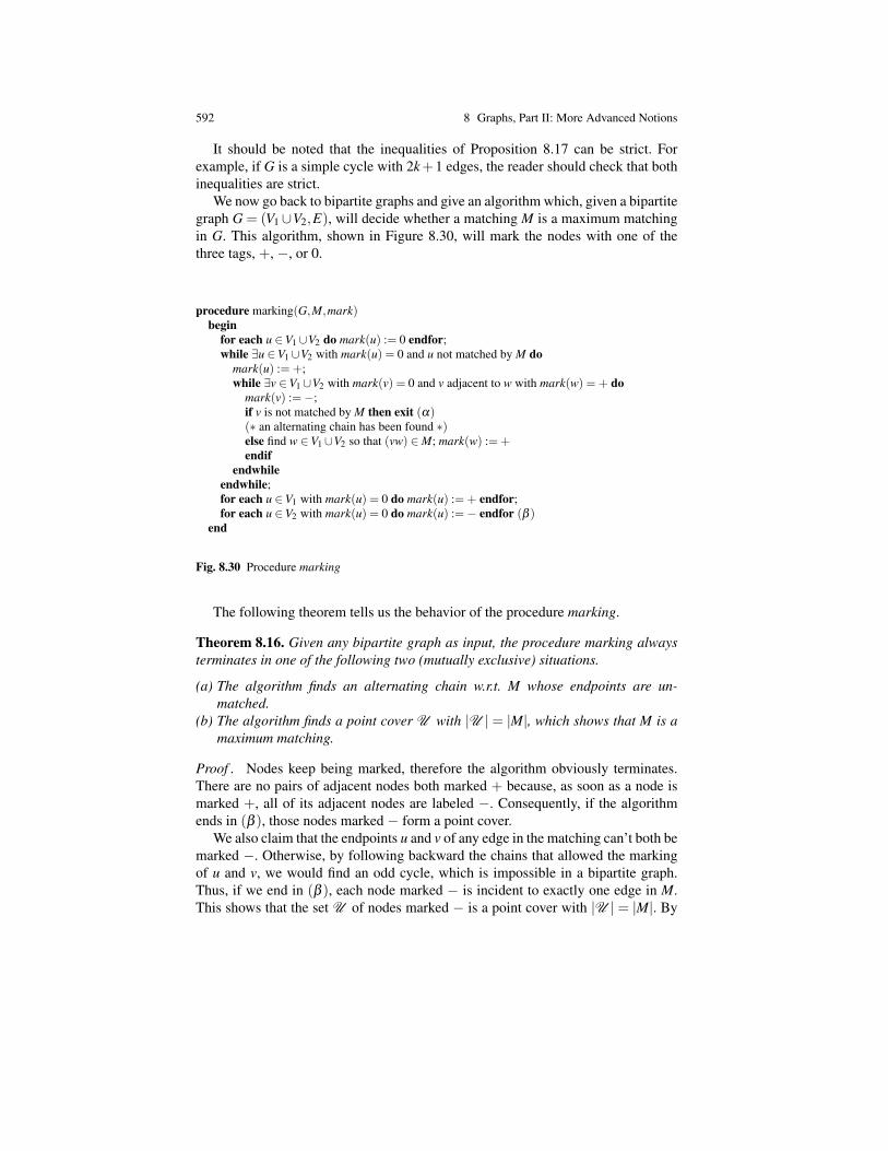
592 8 Graphs, Part II: More Advanced Notions
It should be noted that the inequalities of Proposition 8.17 can be strict. Forexample, if G is a simple cycle with 2k+1 edges, the reader should check that bothinequalities are strict.
We now go back to bipartite graphs and give an algorithm which, given a bipartitegraph G = (V1∪V2,E), will decide whether a matching M is a maximum matchingin G. This algorithm, shown in Figure 8.30, will mark the nodes with one of thethree tags, +, −, or 0.
procedure marking(G,M,mark)begin
for each u ∈V1∪V2 do mark(u) := 0 endfor;while ∃u ∈V1∪V2 with mark(u) = 0 and u not matched by M do
mark(u) :=+;while ∃v ∈V1∪V2 with mark(v) = 0 and v adjacent to w with mark(w) = + do
mark(v) :=−;if v is not matched by M then exit (α)(∗ an alternating chain has been found ∗)else find w ∈V1∪V2 so that (vw) ∈M; mark(w) :=+endif
endwhileendwhile;for each u ∈V1 with mark(u) = 0 do mark(u) :=+ endfor;for each u ∈V2 with mark(u) = 0 do mark(u) :=− endfor (β )
end
Fig. 8.30 Procedure marking
The following theorem tells us the behavior of the procedure marking.
Theorem 8.16. Given any bipartite graph as input, the procedure marking alwaysterminates in one of the following two (mutually exclusive) situations.
(a) The algorithm finds an alternating chain w.r.t. M whose endpoints are un-matched.
(b) The algorithm finds a point cover U with |U | = |M|, which shows that M is amaximum matching.
Proof . Nodes keep being marked, therefore the algorithm obviously terminates.There are no pairs of adjacent nodes both marked + because, as soon as a node ismarked +, all of its adjacent nodes are labeled −. Consequently, if the algorithmends in (β ), those nodes marked − form a point cover.
We also claim that the endpoints u and v of any edge in the matching can’t both bemarked −. Otherwise, by following backward the chains that allowed the markingof u and v, we would find an odd cycle, which is impossible in a bipartite graph.Thus, if we end in (β ), each node marked − is incident to exactly one edge in M.This shows that the set U of nodes marked − is a point cover with |U | = |M|. By

8.5 Matchings, Coverings, Bipartite Graphs 593
Proposition 8.17, we see that U is a minimum point cover and that M is a maximummatching.
If the algorithm ends in (α), by tracing the chain starting from the unmatchednode u, marked − back to the node marked + causing u to be marked, and so on,we find an alternating chain w.r.t. M whose endpoints are not matched. ut
The following important corollaries follow immediately from Theorem 8.16.
Corollary 8.4. In a bipartite graph, the size of a minimum point cover is equal tothe size of maximum matching.
Corollary 8.5. In a bipartite graph, the size of a maximum independent set is equalto the size of a minimum line cover.
Proof . We know from Proposition 8.17 that the complement of a point cover is anindependent set. Consequently, by Corollary 8.4, the size of a maximum indepen-dent set is n−|M|, where M is a maximum matching and n is the number of verticesin G. Now, from Theorem 8.15 (3), for any maximum matching M and any minimalline cover C we have |M|+ |C |= n and so, the size of a maximum independent setis equal to the size of a minimal line cover. ut
We can derive more classical theorems from the above results.Given any graph G = (V,E,st) for any subset of nodes U ⊆V , let
NG(U) = v ∈V −U | (∃u ∈U)(∃e ∈ E)(st(e) = u,v),
be the set of neighbours of U , that is, the set of vertices not in U and adjacent tovertices in U .
Theorem 8.17. (Konig (1931)) For any bipartite graph G= (V1∪V2,E,st) the max-imum size of a matching is given by
minU⊆V1
(|V1−U |+ |NG(U)|).
Proof . This theorem follows from Corollary 8.4 if we can show that every mini-mum point cover is of the form (V1−U)∪NG(U), for some subset U of V1. However,a moment of reflection shows that this is indeed the case. ut
Theorem 8.17 implies another classical result:
Theorem 8.18. (Konig–Hall) For any bipartite graph G = (V1∪V2,E,st) there is amatching M such that all nodes in V1 are matched iff
|NG(U)| ≥ |U | for all U ⊆V1.
Proof . By Theorem 8.17, there is a matching M in G with |M|= |V1| iff
|V1|= minU⊆V1
(|V1−U |+ |NG(U)|) = minU⊆V1
(|V1|+ |NG(U)|− |U |),
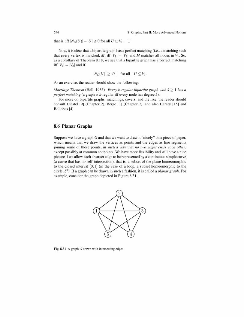
594 8 Graphs, Part II: More Advanced Notions
that is, iff |NG(U)|− |U | ≥ 0 for all U ⊆V1. ut
Now, it is clear that a bipartite graph has a perfect matching (i.e., a matching suchthat every vertex is matched, M, iff |V1| = |V2| and M matches all nodes in V1. So,as a corollary of Theorem 8.18, we see that a bipartite graph has a perfect matchingiff |V1|= |V2| and if
|NG(U)| ≥ |U | for all U ⊆V1.
As an exercise, the reader should show the following.
Marriage Theorem (Hall, 1935) Every k-regular bipartite graph with k ≥ 1 has aperfect matching (a graph is k-regular iff every node has degree k).
For more on bipartite graphs, matchings, covers, and the like, the reader shouldconsult Diestel [9] (Chapter 2), Berge [1] (Chapter 7), and also Harary [15] andBollobas [4].
8.6 Planar Graphs
Suppose we have a graph G and that we want to draw it “nicely” on a piece of paper,which means that we draw the vertices as points and the edges as line segmentsjoining some of these points, in such a way that no two edges cross each other,except possibly at common endpoints. We have more flexibility and still have a nicepicture if we allow each abstract edge to be represented by a continuous simple curve(a curve that has no self-intersection), that is, a subset of the plane homeomorphicto the closed interval [0,1] (in the case of a loop, a subset homeomorphic to thecircle, S1). If a graph can be drawn in such a fashion, it is called a planar graph. Forexample, consider the graph depicted in Figure 8.31.
1
1
5 4
3
2
Fig. 8.31 A graph G drawn with intersecting edges
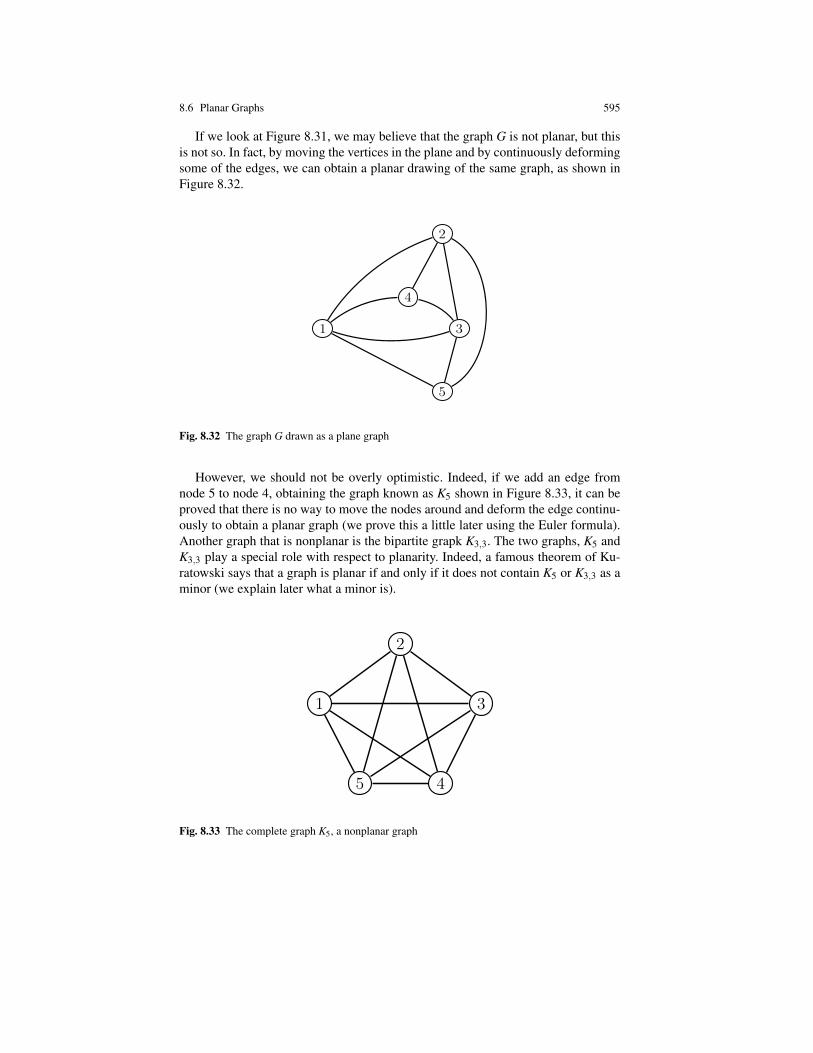
8.6 Planar Graphs 595
If we look at Figure 8.31, we may believe that the graph G is not planar, but thisis not so. In fact, by moving the vertices in the plane and by continuously deformingsome of the edges, we can obtain a planar drawing of the same graph, as shown inFigure 8.32.
1
1
5
4
3
2
Fig. 8.32 The graph G drawn as a plane graph
However, we should not be overly optimistic. Indeed, if we add an edge fromnode 5 to node 4, obtaining the graph known as K5 shown in Figure 8.33, it can beproved that there is no way to move the nodes around and deform the edge continu-ously to obtain a planar graph (we prove this a little later using the Euler formula).Another graph that is nonplanar is the bipartite grapk K3,3. The two graphs, K5 andK3,3 play a special role with respect to planarity. Indeed, a famous theorem of Ku-ratowski says that a graph is planar if and only if it does not contain K5 or K3,3 as aminor (we explain later what a minor is).
1
1
5 4
3
2
Fig. 8.33 The complete graph K5, a nonplanar graph
596 8 Graphs, Part II: More Advanced Notions
Remark: Given n vertices, say 1, . . . ,n, the graph whose edges are all subsetsi, j, with i, j ∈ 1, . . . ,n and i 6= j, is the complete graph on n vertices and isdenoted by Kn (but Diestel uses the notation Kn).
In order to give a precise definition of a planar graph, let us review quicklysome basic notions about curves. A simple curve (or Jordan curve) is any injec-tive continuous function, γ : [0,1]→ R2. Because [0,1] is compact and γ is con-tinuous, it is well known that the inverse f−1 : γ([0,1])→ [0,1] of f is also con-tinuous. So, γ is a homeomorphism between [0,1] and its image γ([0,1]). Witha slight abuse of language we also call the image γ([0,1]) of γ a simple curve.This image is a connected and compact subset of R2. The points a = γ(0) andb = γ(1) are called the boundaries or endpoints of γ (and γ([0,1])). The open subsetγ([0,1])−γ(0),γ(1) is called the interior of γ([0,1]) and is denoted
γ . A con-
tinuous function γ : [0,1]→ R2 such that γ(0) = γ(1) and γ is injective on [0,1) iscalled a simple closed curve or simple loop or closed Jordan curve. Again, by abuseof language, we call the image γ([0,1]) of γ a simple closed curve, and so on. Equiv-alently, if S1 = (x,y) ∈ R2 | x2 + y2 = 1 is the unit circle in R2, a simple closedcurve is any subset of R2 homeomorphic to S1. In this case, we call γ(0) = γ(1) theboundary or base point of γ . The open subset γ([0,1])−γ(0) is called the interiorof γ([0,1]) and is also denoted
γ .
Remark: The notions of simple curve and simple closed curve also make sense ifwe replace R2 by any topological space X , in particular, a surface (In this case, asimple (closed) curve is a continuous injective function γ : [0,1]→ X etc.).
We can now define plane graphs as follows.
Definition 8.21. A plane graph is a pair G = (V,E), where V is a finite set of pointsin R2, E is a finite set of simple curves, and closed simple curves in R2, called edgesand loops, respectively, and satisfying the following properties.
(i) The endpoints of every edge in E are vertices in V and the base point of everyloop is a vertex in V .
(ii) The interior of every edge contains no vertex and the interiors of any two distinctedges are disjoint. Equivalently, every edge contains no vertex except for itsboundaries (base point in the case of a loop) and any two distinct edges intersectonly at common boundary points.
We say that G is a simple plane graph if it has no loops and if different edges havedifferent sets of endpoints
Obviously, a plane graph G = (V,E) defines an “abstract graph” G = (V,E,st)such that
(a) For every simple curve γ ,
st(γ) = γ(0),γ(1).
(b) For every simple closed curve γ ,
st(γ) = γ(0).

8.6 Planar Graphs 597
For simplicity of notation, we usually write G for both the plane graph and theabstract graph associated with G .
Definition 8.22. Given an abstract graph G, we say that G is a planar graph iff thereis some plane graph G and an isomorphism ϕ : G→ G between G and the abstractgraph associated with G . We call ϕ an embedding of G in the plane or a planarembedding of G.
Remarks:
1. If G is a simple planar graph, then by a theorem of Fary, G can be drawn as aplane graph in such a way that the edges are straight line segments (see Grossand Tucker [13], Section 1.6).
2. In view of the remark just before Definition 8.21, given any topological spaceX for instance, a surface, we can define a graph on X as a pair (V,E) where Vis a finite set of points in X and E is a finite set of simple (closed) curves on Xsatisfying the conditions of Definition 8.21.
3. Recall the stereographic projection (from the north pole), σN : (S2−N)→R2, from the sphere, S2 = (x,y,z) ∈ R3 | x2 + y2 + z2 = 1 onto the equatorialplane, z = 0, with N = (0,0,1) (the north pole), given by
σN(x,y,z) =(
x1− z
,y
1− z
).
We know that σN is a homeomorphism, so if ϕ is a planar embedding of a graphG into the plane, then σ
−1N ϕ is an embedding of G into the sphere. Conversely,
if ψ is an embedding of G into the sphere, then σN ψ is a planar embedding ofG. Therefore, a graph can be embedded in the plane iff it can be embedded inthe sphere. One of the nice features of embedding in the sphere is that the sphereis compact (closed and bounded), so the faces (see below) of a graph embeddedin the sphere are all bounded.
4. The ability to embed a graph in a surface other than the sphere broadens theclass of graphs that can be drawn without pairs of intersecting edges (except atendpoints). For example, it is possible to embed K5 and K3,3 (which are knownnot to be planar) into a torus (try it). It can be shown that for every (finite)graph G there is some surface X such that G can be embedded in X . Intuitively,whenever two edges cross on a sphere, by lifting one of the two edges a little bitand adding a “handle” on which the lifted edge lies we can avoid the crossing.An excellent reference on the topic of graphs on surfaces is Gross and Tucker[13].
One of the new ingredients of plane graphs is that the notion of a face makessense. Given any nonempty open subset Ω of the plane R2, we say that two pointsa,b ∈Ω are arcwise connected4 iff there is a simple curve γ such that γ(0) = a and
4 In topology, a space is connected iff it cannot be expressed as the union of two nonempty disjointopen subsets. For open subsets of Rn, connectedness is equivalent to arc connectedness. So it islegitimate to use the term connected.
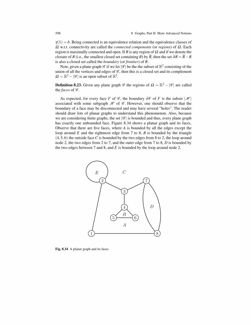
598 8 Graphs, Part II: More Advanced Notions
γ(1) = b. Being connected is an equivalence relation and the equivalence classes ofΩ w.r.t. connectivity are called the connected components (or regions) of Ω . Eachregion is maximally connected and open. If R is any region of Ω and if we denote theclosure of R (i.e., the smallest closed set containing R) by R, then the set ∂R = R−Ris also a closed set called the boundary (or frontier) of R.
Now, given a plane graph G if we let |G | be the the subset of R2 consisting of theunion of all the vertices and edges of G , then this is a closed set and its complementΩ = R2−|G | is an open subset of R2.
Definition 8.23. Given any plane graph G the regions of Ω = R2− |G | are calledthe faces of G .
As expected, for every face F of G , the boundary ∂F of F is the subset |H |associated with some subgraph H of G . However, one should observe that theboundary of a face may be disconnected and may have several “holes”. The readershould draw lots of planar graphs to understand this phenomenon. Also, becausewe are considering finite graphs, the set |G | is bounded and thus, every plane graphhas exactly one unbounded face. Figure 8.34 shows a planar graph and its faces.Observe that there are five faces, where A is bounded by all the edges except theloop around E and the rightmost edge from 7 to 8, B is bounded by the triangle(4,5,6) the outside face C is bounded by the two edges from 8 to 2, the loop aroundnode 2, the two edges from 2 to 7, and the outer edge from 7 to 8, D is bounded bythe two edges between 7 and 8, and E is bounded by the loop around node 2.
1
1
2
3
4
5 6
7
8
A
B
C
D
E
Fig. 8.34 A planar graph and its faces
8.6 Planar Graphs 599
Remarks:
1. Using (inverse) stereographic projection, we see that all the faces of a graphembedded in the sphere are bounded.
2. If a graph G is embedded in a surface S, then the notion of face still makes sense.Indeed, the faces of G are the regions of the open set Ω = S−|G|.
Actually, one should be careful (as usual) not to rely too much on intuition whendealing with planar graphs. Although certain facts seem obvious, they may turn outto be false after closer scrutiny and when they are true, they may be quite hard toprove. One of the best examples of an “obvious” statement whose proof is much lesstrivial than one might expect is the Jordan curve theorem which is actually neededto justify certain “obvious” facts about faces of plane graphs.
Fig. 8.35 Camille Jordan, 1838–1922
Theorem 8.19. (Jordan Curve Theorem) Given any closed simple curve γ in R, thecomplement R2− γ([0,1]), of γ([0,1]) consists of exactly two regions both havingγ([0,1]) as boundary.
Proof . There are several proofs all using machinery (such as homology or differen-tial topology) beyond the scope of these notes. A proof using the notion of windingnumber is given in Guillemin and Pollack [14] (Chapter 2, Section 5) and anotherproof using homology can be found in Munkres [17] (Chapter 4, Section 36). ut
Using Theorem 8.19, the following properties can be proved.
Proposition 8.18. Let G = (V,E) be any plane graph and let e ∈ E be any edge ofG . Then the following properties hold.
(1) For any face F of G , either e⊆ ∂F or ∂F ∩ e= /0.(2) If e lies on a cycle C of G , then e lies on the boundary of exactly two faces of G
and these are contained in distinct faces of C.(3) If e lies on no cycle, then e lies on the boundary of exactly one face of G .
Proof . See Diestel [9], Section 4.2. ut
As corollaries, we also have the following.
600 8 Graphs, Part II: More Advanced Notions
Proposition 8.19. Let G = (V,E) be any plane graph and let F be any face of G .Then, the boundary ∂F of F is a subgraph of G (more accurately, ∂F = |H |, forsome subgraph H of G ).
Proposition 8.20. Every plane forest has a single face.
One of the main theorems about planar graphs is the so-called Euler formula.
Theorem 8.20. (Euler’s formula) Let G be any connected planar graph with n0 ver-tices, n1 edges, and n2 faces. Then, we have
n0−n1 +n2 = 2.
Proof . We proceed by induction on n1. If n1 = 0, the formula is trivially true, asn0 = n2 = 1. Assume the theorem holds for any n1 < n and let G be a connectedplanar graph with n edges. If G has no cycle, then as it is connected, it is a tree,n0 = n+ 1 and n2 = 1, so n0− n1 + n2 = n+ 1− n+ 1 = 2, as desired. Otherwise,let e be some edge of G belonging to a cycle. Consider the graph G′ = (V,E−e);it is still a connected planar graph. Therefore, by the induction hypothesis,
n0− (n1−1)+n′2 = 2.
However, by Proposition 8.18, as e lies on exactly two faces of G, we deduce thatn2 = n′2 +1. Consequently
2 = n0− (n1−1)+n′2 = n0−n1 +1+n2−1 = n0−n1 +n2,
establishing the induction hypothesis. ut
Remarks:
1. Euler’s formula was already known to Descartes in 1640 but the first proof bygiven by Euler in 1752. Poincare generalized it to higher-dimensional polytopes.
2. The numbers n0, n1, and n2 are often denoted by nv, ne, and n f (v for vertex, efor edge and f for face).
3. The quantity n0 − n1 + n2 is called the Euler–Poincare characteristic of thegraph G and it is usually denoted by χG.
4. If a connected graph G is embedded in a surface (orientable) S, then we stillhave an Euler formula of the form
n0−n1 +n2 = χ(S) = 2−2g,
where χ(S) is a number depending only on the surface S, called the Euler–Poincare characteristic of the surface and g is called the genus of the surface.It turns out that g ≥ 0 is the number of “handles” that need to be glued to thesurface of a sphere to get a homeomorphic copy of the surface S. For more onthis fascinating subject, see Gross and Tucker [13].
8.6 Planar Graphs 601
Fig. 8.36 Rene Descartes, 1596–1650 (left) and Leonhard Euler, 1707–1783 (right)
It is really remarkable that the quantity n0− n1 + n2 is independent of the waya planar graph is drawn on a sphere (or in the plane). A neat application of Euler’sformula is the proof that there are only five regular convex polyhedra (the so-calledplatonic solids). Such a proof can be found in many places, for instance, Berger [2]and Cromwell [8]. It is easy to generalize Euler’s formula to planar graphs that arenot necessarily connected.
Theorem 8.21. Let G be any planar graph with n0 vertices, n1 edges, n2 faces, andc connected components. Then, we have
n0−n1 +n2 = c+1.
Proof . Reduce the proof of Theorem 8.21 to the proof of Theorem 8.20 by addingvertices and edges between connected components to make G connected. Detailsare left as an exercise. ut
Using the Euler formula we can now prove rigorously that K5 and K3,3 are notplanar graphs. For this, we need the following fact.
Proposition 8.21. If G is any simple, connected, plane graph with n1 ≥ 3 edges andn2 faces, then
2n1 ≥ 3n2.
Proof . Let F(G) be the set of faces of G. Because G is connected, by Proposition8.18 (2), every edge belongs to exactly two faces. Thus, if sF is the number of sidesof a face F of G, we have
∑F∈F(G)
sF = 2n1.
Furthermore, as G has no loops, no parallel edges, and n0 ≥ 3, every face has at leastthree sides; that is, sF ≥ 3. It follows that
2n1 = ∑F∈F(G)
sF ≥ 3n2,
as claimed. ut

602 8 Graphs, Part II: More Advanced Notions
The proof of Proposition 8.21 shows that the crucial constant on the right-handside of the inequality is the the minimum length of all cycles in G. This number iscalled the girth of the graph G. The girth of a graph with a loop is 1 and the girthof a graph with parallel edges is 2. The girth of a tree is undefined (or infinite).Therefore, we actually proved the next proposition.
Proposition 8.22. If G is any connected plane graph with n1 edges and n2 faces andG is not a tree, then
2n1 ≥ girth(G)n2.
Corollary 8.6. If G is any simple, connected, plane graph with n≥ 3 nodes then Ghas at most 3n−6 edges and 2n−4 faces.
Proof . By Proposition 8.21, we have 2n1 ≥ 3n2, where n1 is the number of edgesand n2 is the number of faces. So, n2 ≤ 2
3 n1 and by Euler’s formula
n−n1 +n2 = 2,
we get
n−n1 +23
n1 ≥ 2;
that is,
n− 13
n1 ≥ 2,
namely n1 ≤ 3n−6. Using n2 ≤ 23 n1, we get n2 ≤ 2n−4. ut
Corollary 8.7. The graphs K5 and K3,3 are not planar.
Proof . We proceed by contradiction. First, consider K5. We have n0 = 5 and K5has n1 = 10 edges. On the other hand, by Corollary 8.6, K5 should have at most3×5−6 = 15−6 = 9 edges, which is absurd.
Next, consider K3,3. We have n0 = 6 and K3,3 has n1 = 9 edges. By the Eulerformula, we should have
n2 = 9−6+2 = 5.
Now, as K3,3 is bipartite, it does not contain any cycle of odd length, and so eachface has at least four sides, which implies that
2n1 ≥ 4n2
(because the girth of K3,3 is 4.) So, we should have
18 = 2 ·9≥ 4 ·5 = 20,
which is absurd. ut
Another important property of simple planar graph is the following.

8.6 Planar Graphs 603
Proposition 8.23. If G is any simple planar graph, then there is a vertex u such thatdG(u)≤ 5.
Proof . If the property holds for any connected component of G, then it holds forG, so we may assume that G is connected. We already know from Proposition 8.21that 2n1 ≥ 3n2; that is,
n2 ≤23
n1. (∗)
If dG(u)≥ 6 for every vertex u, as ∑u∈V dG(u) = 2n1, then 6n0 ≤ 2n1; that is, n0 ≤n1/3. By Euler’s formula, we would have
n2 = n1−n0 +2≥ n1−13
n1 +2 >23
n1,
contradicting (∗). ut
Remarkably, Proposition 8.23 is the key ingredient in the proof that every planargraph is 5-colorable.
Theorem 8.22. (5-Color Theorem) Every planar graph G is 5-colorable.
Proof . Clearly, parallel edges and loops play no role in finding a coloring of thevertices of G, so we may assume that G is a simple graph. Also, the property isclear for graphs with less than 5 vertices. We proceed by induction on the numberof vertices m. By Proposition 8.23, the graph G has some vertex u0 with dG(u)≤ 5.By the induction hypothesis, we can color the subgraph G′ induced by V −u0with 5 colors. If d(u0)< 5, we can color u0 with one of the colors not used to colorthe nodes adjacent to u0 (at most 4) and we are done. So, assume dG(u0) = 5 andlet v1, . . . ,v5 be the nodes adjacent to u0 and encountered in this order when werotate counterclockwise around u0 (see Figure 8.37). If v1, . . . ,v5 are not coloredwith different colors, again, we are done.
Otherwise, by the induction hypothesis, let X1, . . . ,X5 be a coloring of G′ and,by renaming the Xis if necessary, assume that vi ∈ Xi, for i = 1, . . . ,5. There are twocases.
(1) There is no chain from v1 to v3 whose nodes belong alternately to X1 and X2.If so, v1 and v3 must belong to different connected components of the subgraphH ′ of G′ induced by X1 ∪X2. Then, we can permute the colors 1 and 3 in theconnected component of H ′ that contains v3 and color u0 with color 3.
(2) There is a chain from v1 to v3 whose nodes belong alternately to X1 and X2. Inthis case, as G is a planar graph, there can’t be any chain from v2 to v4 whosenodes belong alternately to X2 and X4. So, v2 and v4 do not belong to the sameconnected component of the subgraph H ′′ of G′ induced by X2∪X4. But then, wecan permute the colors 2 and 4 in the connected component of H ′′ that containsv4 and color u0 with color 4. ut

604 8 Graphs, Part II: More Advanced Notions
1
v2
v3 v4
v5
v1
u0
Fig. 8.37 The five nodes adjacent to u0
Theorem 8.22 raises a very famous problem known as the four-color problem:Can every planar graph be colored with four colors?
This question was apparently first raised by Francis Guthrie in 1850, commu-nicated to De Morgan by Guthrie’s brother Frederick in 1852, and brought to theattention of a wider public by Cayley in 1878. In the next hundred years, several in-correct proofs were proposed and this problem became known as the four-color con-jecture. Finally, in 1977, Appel and Haken gave the first “proof” of the four-colorconjecture. However, this proof was somewhat controversial for various reasons,one of the reasons being that it relies on a computer program for checking a largenumber of unavoidable configurations. Appel and Haken subsequently publisheda 741-page paper correcting a number of errors and addressing various criticisms.More recently (1997) a much shorter proof, still relying on a computer program, buta lot easier to check (including the computer part of it) has been given by Robert-son, Sanders, Seymour, and Thomas [19]. For more on the four-color problem, seeDiestel [9], Chapter 5, and the references given there.
Let us now go back to Kuratowski’s criterion for nonplanarity. For this it is usefulto introduce the notion of edge contraction in a graph.
Definition 8.24. Let G = (V,E,st) be any graph and let e be any edge of G. Thegraph obtained by contracting the edge e into a new vertex ve is the graph G/e =(V ′,E ′,st ′) with V ′ = (V − st(e))∪ ve, where ve is a new node (ve /∈ V ); E ′ =E−e; and with
st ′(e′) =
st(e′) if st(e′)∩ st(e) = /0ve if st(e′) = st(e)u,ve if st(e′)∩ st(e) = z and st(e′) = u,z with u 6= zve if st(e′) = x or st(e′) = y with st(e) = x,y.
If G is a simple graph, then we need to eliminate parallel edges and loops. In, thiscase, e = x,y and G/e = (V ′,E ′,st) is defined so that V ′ = (V −x,y)∪ve,where ve is a new node and
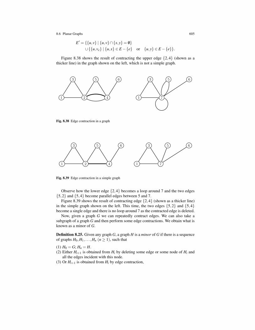
8.6 Planar Graphs 605
E ′ = u,v | u,v∩x,y= /0∪u,ve | u,x ∈ E−e or u,y ∈ E−e.
Figure 8.38 shows the result of contracting the upper edge 2,4 (shown as athicker line) in the graph shown on the left, which is not a simple graph.
1
1 2
3
4
5 6
1 7
3 5 6
Fig. 8.38 Edge contraction in a graph
1
1 2
3
4
5 6
1 7
3 5 6
Fig. 8.39 Edge contraction in a simple graph
Observe how the lower edge 2,4 becomes a loop around 7 and the two edges5,2 and 5,4 become parallel edges between 5 and 7.
Figure 8.39 shows the result of contracting edge 2,4 (shown as a thicker line)in the simple graph shown on the left. This time, the two edges 5,2 and 5,4become a single edge and there is no loop around 7 as the contracted edge is deleted.
Now, given a graph G we can repeatedly contract edges. We can also take asubgraph of a graph G and then perform some edge contractions. We obtain what isknown as a minor of G.
Definition 8.25. Given any graph G, a graph H is a minor of G if there is a sequenceof graphs H0,H1, . . . ,Hn (n≥ 1), such that
(1) H0 = G; Hn = H.(2) Either Hi+1 is obtained from Hi by deleting some edge or some node of Hi and
all the edges incident with this node.(3) Or Hi+1 is obtained from Hi by edge contraction,

606 8 Graphs, Part II: More Advanced Notions
with 0 ≤ i ≤ n− 1. If G is a simple graph, we require that edge contractions be ofthe second type described in Definition 8.24, so that H is a simple graph.
It is easily shown that the minor relation is a partial order on graphs (and sim-ple graphs). Now, the following remarkable theorem originally due to Kuratowskicharacterizes planarity in terms of the notion of minor:
Fig. 8.40 Kazimierz Kuratowski, 1896–1980
Theorem 8.23. (Kuratowski, 1930) For any graph G, the following assertions areequivalent.
(1) G is planar.(2) G contains neither K5 nor K3,3 as a minor.
Proof . The proof is quite involved. The first step is to prove the theorem for 3-connected graphs. (A graph, G = (V,E), is h-connected iff |V | > h and iff everygraph obtained by deleting any set S⊆V of nodes with |S|< h and the edges incidentto these node is still connected. So, a 1-connected graph is just a connected graph.)We refer the reader to Diestel [9], Section 4.4, for a complete proof. ut
Another way to state Kuratowski’s theorem involves edge subdivision, an oper-ation of independent interest. Given a graph G = (V,E,st) possibly with loops andparallel edges, the result of subdividing an edge e consists in creating a new vertexve, deleting the edge e, and adding two new edges from ve to the old endpoints of e(possibly the same point). Formally, we have the following definition.
Definition 8.26. Given any graph G = (V,E,st) for any edge e ∈ E, the result ofsubdividing the edge e is the graph G′ = (V ∪ve,(E−e)∪e1,e2,st ′), whereve is a new vertex and e1,e2 are new edges, st ′(e′) = st(e′) for all e′ ∈ E−e andif st(e) = u,v (u = v is possible), then st ′(e1) = ve,u and st ′(e2) = ve,v. Ifa graph G′ is obtained from a graph G by a sequence of edge subdivisions, we saythat G′ is a subdivision of G.
Observe that by repeatedly subdividing edges, any graph can be transformed intoa simple graph. Given two graphs G and H, we say that G and H are homeomorphic

8.6 Planar Graphs 607
1
Fig. 8.41 Two homeomorphic graphs
iff they have respective subdivisions G′ and H ′ that are isomorphic graphs. The ideais that homeomorphic graphs “look the same,” viewed as topological spaces. Figure8.41 shows an example of two homeomorphic graphs.
A graph H that has a subdivision H ′, which is a subgraph of some graph G, iscalled a topological minor of G. Then, it is not hard to show (see Diestel [9], Chapter4, or Gross and Tucker [13], Chapter 1) that Kuratowski’s theorem is equivalent tothe statement
A graph G is planar iff it does not contain any subgraph homeomorphic to eitherK5 or K3,3 or, equivalently, if it has has neither K5 nor K3,3 as a topological minor.
Another somewhat surprising characterization of planarity involving the conceptof cycle space over F2 (see Definition 8.4 and the Remarks after Theorem 8.2) anddue to MacLane is the following.
Fig. 8.42 Saunders Mac Lane, 1909–2005
Theorem 8.24. (MacLane, 1937) A graph G is planar iff its cycle space F over F2has a basis such that every edge of G belongs to at most two cycles of this basis.
Proof . See Diestel [9], Section 4.4. ut
We conclude this section on planarity with a brief discussion of the dual graphof a plane graph, a notion originally due to Poincare. Duality can be generalizedto simplicial complexes and relates Voronoi diagrams and Delaunay triangulations,two very important tools in computational geometry.
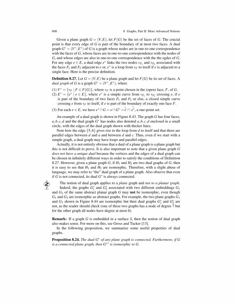
608 8 Graphs, Part II: More Advanced Notions
Given a plane graph G = (V,E), let F(G) be the set of faces of G. The crucialpoint is that every edge of G is part of the boundary of at most two faces. A dualgraph G∗ = (V ∗,E∗) of G is a graph whose nodes are in one-to-one correspondencewith the faces of G, whose faces are in one-to-one correspondence with the nodes ofG, and whose edges are also in one-to-one correspondence with the the egdes of G.For any edge e ∈ E, a dual edge e∗ links the two nodes vF1 and vF2 associated withthe faces F1 and F2 adjacent to e or, e∗ is a loop from vF to itself if e is adjacent to asingle face. Here is the precise definition.
Definition 8.27. Let G = (V,E) be a plane graph and let F(G) be its set of faces. Adual graph of G is a graph G∗ = (V ∗,E∗), where
(1) V ∗ = vF | F ∈ F(G), where vF is a point chosen in the (open) face, F , of G.(2) E∗ = e∗ | e ∈ E, where e∗ is a simple curve from vF1 to vF2 crossing e, if e
is part of the boundary of two faces F1 and F2 or else, a closed simple curvecrossing e from vF to itself, if e is part of the boundary of exactly one face F .
(3) For each e ∈ E, we have e∗∩G = e∩G∗ =e ∩
e∗, a one-point set.
An example of a dual graph is shown in Figure 8.43. The graph G has four faces,a,b,c,d and the dual graph G∗ has nodes also denoted a,b,c,d enclosed in a smallcircle, with the edges of the dual graph shown with thicker lines.
Note how the edge 5,6 gives rise to the loop from d to itself and that there areparallel edges between d and a and between d and c. Thus, even if we start with asimple graph, a dual graph may have loops and parallel edges.
Actually, it is not entirely obvious that a dual of a plane graph is a plane graph butthis is not difficult to prove. It is also important to note that a given plane graph Gdoes not have a unique dual because the vertices and the edges of a dual graph canbe chosen in infinitely different ways in order to satisfy the conditions of Definition8.27. However, given a plane graph G, if H1 and H2 are two dual graphs of G, thenit is easy to see that H1 and H2 are isomorphic. Therefore, with a slight abuse oflanguage, we may refer to “the” dual graph of a plane graph. Also observe that evenif G is not connected, its dual G∗ is always connected.
The notion of dual graph applies to a plane graph and not to a planar graph.Indeed, the graphs G∗1 and G∗2 associated with two different embeddings G1
and G2 of the same abstract planar graph G may not be isomorphic, even thoughG1 and G2 are isomorphic as abstract graphs. For example, the two plane graphs G1and G2 shown in Figure 8.44 are isomorphic but their dual graphs G∗1 and G∗2 arenot, as the reader should check (one of these two graphs has a node of degree 7 butfor the other graph all nodes have degree at most 6).
Remark: If a graph G is embedded in a surface S, then the notion of dual graphalso makes sense. For more on this, see Gross and Tucker [13].
In the following proposition, we summarize some useful properties of dualgraphs.
Proposition 8.24. The dual G∗ of any plane graph is connected. Furthermore, if Gis a connected plane graph, then G∗∗ is isomorphic to G.

8.6 Planar Graphs 609
1
1
2
3
4
5
66
a
b
c
d
Fig. 8.43 A graph and its dual graph
1
1 2
3 4
5
6 1
2
3 4
5
6
Fig. 8.44 Two isomorphic plane graphs whose dual graphs are not isomorphic
Proof . Left as an exercise. ut
With a slight abuse of notation we often write G∗∗ = G (when G is connected). Aplane graph G whose dual G∗ is equal to G (i.e., isomorphic to G) is called self-dual.For example, the plane graph shown in Figure 8.45 (the projection of a tetrahedronon the plane) is self-dual.
The duality of plane graphs is also reflected algebraically as a duality betweentheir cycle spaces and their cut spaces (over F2).
Proposition 8.25. If G is any connected plane graph G, then the following proper-ties hold.
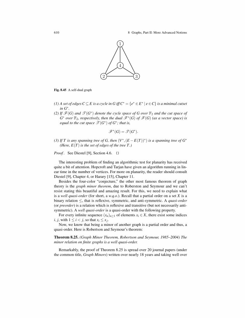
610 8 Graphs, Part II: More Advanced Notions
1
1
2 3
4
Fig. 8.45 A self-dual graph
(1) A set of edges C⊆ E is a cycle in G iff C∗ = e∗ ∈ E∗ | e∈C is a minimal cutsetin G∗.
(2) If F (G) and T (G∗) denote the cycle space of G over F2 and the cut space ofG∗ over F2, respectively, then the dual F ∗(G) of F (G) (as a vector space) isequal to the cut space T (G∗) of G∗; that is,
F ∗(G) = T (G∗).
(3) If T is any spanning tree of G, then (V ∗,(E−E(T ))∗) is a spanning tree of G∗
(Here, E(T ) is the set of edges of the tree T .)
Proof . See Diestel [9], Section 4.6. ut
The interesting problem of finding an algorithmic test for planarity has receivedquite a bit of attention. Hopcroft and Tarjan have given an algorithm running in lin-ear time in the number of vertices. For more on planarity, the reader should consultDiestel [9], Chapter 4, or Harary [15], Chapter 11.
Besides the four-color “conjecture,” the other most famous theorem of graphtheory is the graph minor theorem, due to Roberston and Seymour and we can’tresist stating this beautiful and amazing result. For this, we need to explain whatis a well quasi-order (for short, a w.q.o.). Recall that a partial order on a set X is abinary relation ≤, that is reflexive, symmetric, and anti-symmetric. A quasi-order(or preorder) is a relation which is reflexive and transitive (but not necessarily anti-symmetric). A well quasi-order is a quasi-order with the following property.
For every infinite sequence (xn)n≥1 of elements xi ∈ X , there exist some indicesi, j, with 1≤ i < j, so that xi ≤ x j.
Now, we know that being a minor of another graph is a partial order and thus, aquasi-order. Here is Robertson and Seymour’s theorem:
Theorem 8.25. (Graph Minor Theorem, Robertson and Seymour, 1985–2004) Theminor relation on finite graphs is a well quasi-order.
Remarkably, the proof of Theorem 8.25 is spread over 20 journal papers (underthe common title, Graph Minors) written over nearly 18 years and taking well over
8.7 Summary 611
Fig. 8.46 Paul D. Seymour, 1950– (left) and G Neil Robertson, 1938– (right)
500 pages! Many original techniques had to be invented to come up with this proof,one of which is a careful study of the conditions under which a graph can be em-bedded in a surface and a “Kuratowski-type” criterion based on a finite family of“forbidden graphs.” The interested reader is urged to consult Chapter 12 of Diestel[9] and the references given there.
A precursor of the graph minor theorem is a theorem of Kruskal (1960) thatapplies to trees. Although much easier to prove than the graph minor theorem, theproof fo Kruskal’s theorem is very ingenious. It turns out that there are also someinteresting connections between Kruskal’s theorem and proof theory, due to HarveyFriedman. A survey on this topic can be found in Gallier [10].
8.7 Summary
This chapter delves more deeply into graph theory. We begin by defining two fun-damental vector spaces associated with a finite directed graph G, the cycle spaceor flow space F (G), and the cocycle space or tension space (or cut space) T (G).These spaces turn out to be orthogonal. We explain how to find bases of these spacesin terms of spanning trees and cotrees and we determine the dimensions of thesespaces in terms of the number of edges, the number of vertices, and the numberof connected components of the graph. A pretty lemma known as the arc coloringlemma (due to Minty) plays a crucial role in the above presentation which is heavilyinspired by Berge [1] and Sakarovitch [20]. We discuss the incidence matrix and theadjacency matrix of a graph and explain how the spaces of flows and tensions canbe recovered from the incidence matrix. We also define the Laplacian of a graph.Next, we discuss briefly Eulerian and Hamiltonian cycles. We devote a long sectionto flow problems and in particular to the max-flow min-cut theorem and some of itsvariants. The proof of the max-flow min-cut theorem uses the arc-coloring lemmain an interesting way, as indicated by Sakarovitch [20]. Matchings, coverings, andbipartite graphs are briefly treated. We conclude this chapter with a discussion ofplanar graphs. Finally, we mention two of the most famous theorems of graph the-

612 8 Graphs, Part II: More Advanced Notions
ory: the four color-conjecture (now theorem, or is it?) and the graph minor theorem,due to Robertson and Seymour.
• We define the representative vector of a cycle and then the notion of Γ -cycle Γ ,representative vector of a Γ -cycle γ(Γ ), a Γ -circuit, and a simple Γ -cycle.
• Next, we define a cocycle (or cutset) Ω , its representative vector ω(Ω), a co-circuit, and a simple cocycle.
• We define a cutset.• We prove several characterizations of simple cocycles.• We prove the fundamental fact that the representative vectors of Γ -cycles and
cocycles are orthogonal.• We define the cycle space or flow space F (G), and the cocycle space or tension
space (or cut space), T (G).• We prove a crucial technical result: the arc coloring lemma (due to Minty).• We derive various consequences of the arc-coloring lemma, including the fact
that every edge of a finite digraph either belongs to a simple circuit or a simplecocircuit but not both.
• We define a cotree and give a useful characterization of them.• We prove the main theorem of Section 8.1 (Theorem 8.2), namely, we compute
the dimensions of the spaces F (G) and T (G), and we explain how to computebases of these spaces in terms of spanning trees and cotrees.
• We define the cyclomatic number and the cocyclomatic number of a (di)graph.• We remark that the dimension of F (G) is the dimension of the first homol-
ogy group of the graph and that the Euler–Poincare characteristic formula is aconsequence of the formulae for the dimensions of F (G) and T (G).
• We give some useful characterizations of flows and tensions.• We define the incidence matrix D(G) of a directed graph G (without parallel
edges or loops).• We characterize F (G) and T (G) in terms of the incidence matrix.• We prove a theorem of Poincare about nonsingular submatrices of D which
shows that D is totally unimodular.• We define the adjacency matrix A(G) of a graph.• We prove that DD> = ∆ −A, where ∆ is the diagonal matrix consisting of the
degrees of the vertices.• We define DD> as the Laplacian of the graph.• The study of the matrix DD>, especially its eigenvalues, is an active area of
research called spectral graph theory.• We define an Euler cycle and an Euler circuit.• We prove a simple characterization of the existence of an Euler cycle (or an
Euler circuit).• We define a Hamiltonian cycle and a Hamiltonian circuit.• We mention that the Hamiltonian cycle problem is NP-complete.• We define a network (or flow network), a digraph together with a capacity func-
tion (or cost function).• We define the notion of flow, of value of a flow, and state the network flow
problem.

8.7 Summary 613
• We define the notion of vs-vt -cut and of capacity of a vs-vt -cut.• We prove a basic result relating the maximum value of a flow to the minimum
capacity of a vs-vt -cut.• We define a minimum vs-vt -cut or minimum cut.• We prove that in any network there is a flow of maximum value.• We prove the celebrated max-flow min-cut theorem due to Ford and Fulkerson
using the arc coloring lemma.• We define a flow augmenting chain.• We describe the algorithm maxflow and prove its correctness (provided that it
terminates).• We give a sufficient condition for the termination of the algorithm maxflow (all
the capacities are multiples of some given number).• The above criterion implies termination of maxflow if all the capacities are inte-
gers and that the algorithm will output some maximum flow with integer capac-ities.
• In order to improve the complexity of the algorithm maxflow we define a resid-ual network.
• We briefly discuss faster algorithms for finding a maximum flow. We define apreflow and mention “preflow-push relabel algorithms.”
• We present a few applications of the max-flow min-cut theorem, such as a the-orem due to Menger on edge-disjoint paths.
• We discuss channeled flows and state a theorem due to Hoffman that character-izes when a channeled flow exists.
• We define a bottleneck and give an algorithm for finding a channeled flow.• We state a max-flow min-cut theorem for channeled flows.• We conclude with a discussion of a variation of the max flow problem consid-
ered in Cormen et al. [7] (Chapter 26).• We define a bipartite graph and a maximum matching.• We define the complete bipartite graphs, Km,n.• We explain how the maxflow algorithm can be used to find a maximum match-
ing.• We define a k-coloring of a graph, when a graph is k-colorable and the chromatic
number of a graph.• We define the incidence matrix of a nonoriented graph and we characterize a
bipartite graph in terms of its incidence matrix.• We define a matching in a graph, a matched vertex, and a perfect matching.• We define an alternating chain.• We characterize a maximal matching in terms of alternating chains.• We define a line cover and a minimum line cover.• We prove a relationship between maximum matchings and minimum line cov-
ers.• We define an independent (or stable) set of nodes and a maximum independent
set.• We define a point cover (or transversal) and a minimum point cover.
614 8 Graphs, Part II: More Advanced Notions
• We go back to bipartite graphs and describe a marking procedure that decideswhether a matching is a maximum matching.
• As a corollary, we derive some properties of minimum point covers, maximummatchings, maximum independent sets, and minimum line covers in a bipartitegraph.
• We also derive two classical theorems about matchings in a bipartite graph dueto Konig and Konig–Hall and we state the marriage theorem (due to Hall).
• We introduce the notion of a planar graph.• We define the complete graph on n vertices Kn.• We define a Jordan curve (or a simple curve), endpoints (or boundaries) of a
simple curve, a simple loop or closed Jordan curve, a base point and the interiorof a closed Jordan curve.
• We define rigorously a plane graph and a simple plane graph.• We define a planar graph and a planar embedding.• We define the stereographic projection onto the sphere. A graph can be embed-
ded in the plane iff it can be embedded in the sphere.• We mention the possibility of embedding a graph into a surface.• We define the connected components (or regions) of an open subset of the plane
as well as its boundary.• We define the faces of plane graph.• We state the Jordan curve theorem• We prove Euler’s formula for connected planar graphs and talk about the Euler–
Poincare characteristic of a planar graph.• We generalize Euler’s formula to planar graphs that are not necessarily con-
nected.• We define the girth of a graph and prove an inequality involving the girth for
connected planar graphs.• As a consequence, we prove that K5 and K3,3 are not planar.• We prove that every planar graph is 5-colorable.• We mention the four-color conjecture.• We define edge contraction and define a minor of a graph.• We state Kuratowski’s theorem characterizing planarity of a graph in terms of
K3 and K3,3.• We define edge subdivision and state another version of Kuratowski’s theorem
in terms of minors.• We state MacLane’s criterion for planarity of a graph in terms of a property of
its cycle space over F2.• We define the dual graph of a plane graph and state some results relating the
dual and the bidual of a graph to the original graph.• We define a self-dual graph.• We state a theorem relating the flow and tension spaces of a plane graph and its
dual.• We conclude with a discussion of the graph minor theorem.• We define a quasi-order and a well quasi-order.• We state the graph minor theorem due to Robertson and Seymour.
8.7 Problems 615
Problems
8.1. Recall from Problem 4.14 that an undirected graph G is h-connected (h ≥ 1)iff the result of deleting any h− 1 vertices and the edges adjacent to these verticesdoes not disconnect G. Prove that if G is an undirected graph and G is 2-connected,then there is an orientation of the edges of G for which G (as an oriented graph) isstrongly connected.
8.2. Given a directed graph G = (V,E,s, t) prove that a necessary and sufficientcondition for a subset of edges E ′ ⊆ E to be a cocycle of G is that it is possible tocolor the vertices of G with two colors so that:
1. The endpoints of every edge in E ′ have different colors.2. The endpoints of every edge in E−E ′ have the same color.
Under which condition do the edges of the graph consitute a cocycle? If the graphis connected (as an undirected graph), under which condition is E ′ a simple cocycle?
8.3. Prove that if G is a strongly connected graph, then its flow space F (G) has abasis consisting of representative vectors of circuits.Hint. Use induction on the number of vertices.
8.4. Prove that if the graph G has no circuit, then its tension space T (G) has a basisconsisting of representative vectors of cocircuits.Hint. Use induction on the number of vertices.
8.5. Let V be a subspace of Rn. The support of a vector v ∈V is defined by
S(v) = i ∈ 1, . . . ,n | vi 6= 0.
A vector v ∈V is said to be elementary iff it has minimal support, which means thatfor any v′ ∈V , if S(v′)⊆ S(v) and S(v′) 6= S(v), then v′ = 0.
(a) Prove that if any two elementary vectors of V have the same support, thenthey are collinear.
(b) Let f be an elementary vector in the flow space F (G) of G (respectively, τ
be an elementary vector in the tension space, T (G), of G). Prove that
f = λγ (respectively, τ = µω),
with λ ,µ ∈ R and γ (respectively, ω) is the representative vector of a simple cycle(respectively, of a simple cocycle) of G.
(c) For any m×n matrix, A, let V be the subspace given by
V = x ∈ Rn | Ax = 0.
Prove that the following conditions are equivalent.
(i) A is totally unimodular.(ii) For every elementary vector x ∈V , whenever xi 6= 0 and x j 6= 0, then |xi|= |x j|.
616 8 Graphs, Part II: More Advanced Notions
8.6. Given two m×m matrices with entries either 0 or 1, define A+B as the matrixwhose (i, j)th entry is the Boolean sum ai j ∨bi j and AB as the matrix whose (i, j)thentry is given by
(ai1∧b1 j)∨ (ai2∧b2 j)∨·· ·∨ (aim∧bm j);
that is, interpret 0 as false, 1 as true, + as or and · as and.(i) Prove that
Aki j =
1 iff there is a path of length k from vi to v j0 otherwise.
(ii) LetBk = A+A2 + · · ·+Ak.
Prove that there is some k0 so that
Bn+k0 = Bk0 ,
for all n≥ 1. Describe the graph associated with Bk0 .
8.7. Let G be an undirected graph known to have an Euler cycle. The principle ofFleury’s algorithm for finding an Euler cycle in G is the following.
1. Pick some vertex v as starting point and set k = 1.2. Pick as the kth edge in the cycle being constructed an edge e adjacent to v whose
deletion does not disconnect G. Update G by deleting edge e and the endpointof e different from v and set k := k+1.
Prove that if G has an Euler cycle, then the above algorithm outputs an Eulercycle.
8.8. Recall that Km denotes the (undirected) complete graph on m vertices.(a) For which values of m does Km contain an Euler cycle?Recall that Km,n denotes the (undirected) complete bipartite graph on m+n ver-
tices.(b) For which values of m and n does Km,n contain an Euler cycle?
8.9. Prove that the graph shown in Figure 8.47 has no Hamiltonian.
8.10. Prove that the graph shown in Figure 8.48 and known as Petersen’s graphsatisfies the conditions of Proposition 8.12, yet this graph has no Hamiltonian.
8.11. Prove that if G is a simple undirected graph with n vertices and if n ≥ 3 andthe degree of every vertex is at least n/2, then G is Hamiltonian (this is known asDirac’s Theorem).
8.12. Find a minimum cut separating vs and vt in the network shown in Figure 8.49:
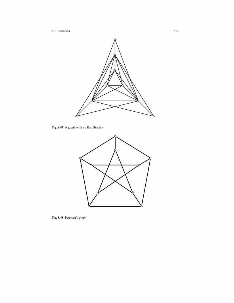
8.7 Problems 617
1
Fig. 8.47 A graph with no Hamiltonian
1
Fig. 8.48 Petersen’s graph
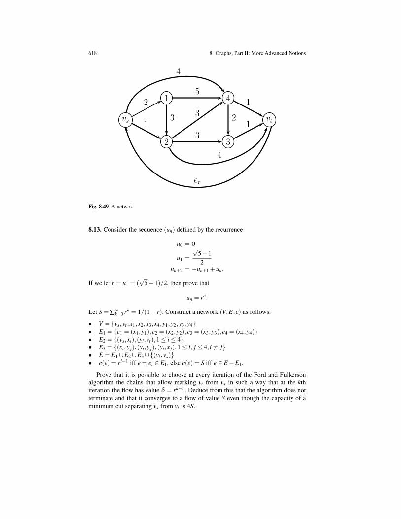
618 8 Graphs, Part II: More Advanced Notions
1
vs
1
2 3
4
vt1
2
3
3
5
3 2
1
1
4
4
er
Fig. 8.49 A netwok
8.13. Consider the sequence (un) defined by the recurrence
u0 = 0
u1 =
√5−12
un+2 = −un+1 +un.
If we let r = u1 = (√
5−1)/2, then prove that
un = rn.
Let S = ∑∞k=0 rn = 1/(1− r). Construct a network (V,E,c) as follows.
• V = vs,vt ,x1,x2,x3,x4,y1,y2,y3,y4• E1 = e1 = (x1,y1),e2 = (x2,y2),e3 = (x3,y3),e4 = (x4,y4)• E2 = (vs,xi),(yi,vt),1≤ i≤ 4• E3 = (xi,y j),(yi,y j),(yi,x j),1≤ i, j ≤ 4, i 6= j• E = E1∪E2∪E3∪(vt ,vs)• c(e) = ri−1 iff e = ei ∈ E1, else c(e) = S iff e ∈ E−E1.
Prove that it is possible to choose at every iteration of the Ford and Fulkersonalgorithm the chains that allow marking vt from vs in such a way that at the kthiteration the flow has value δ = rk−1. Deduce from this that the algorithm does notterminate and that it converges to a flow of value S even though the capacity of aminimum cut separating vs from vt is 4S.
8.7 Problems 619
8.14. Let E = e1, . . . ,em be a finite set and let S = S1, . . . ,Sn be a family of finitesubsets of E. A set T = ei1 , . . . ,ein of distinct elements of E is a transversal for S(also called a system of distinct representatives for S) iff
ei j ∈ S j, j = 1, . . . ,n.
Hall’s theorem states that the family S has a transversal iff for every subset I ⊆1, . . . ,n we have
|I| ≤∣∣∣∣∣⋃i∈I
Si
∣∣∣∣∣ .(a) Prove that the above condition is necessary.
(b) Associate a bipartite graph with S and T and use Theorem 8.18 to prove thatthe above condition is indeed sufficient.
8.15. Let G be a directed graph without any self-loops or any cicuits (G is acyclic).Two vertices u,v, are independent (or incomparable) iff they do not belong to anypath in G. A set of paths (possibly consisting of a single vertex) covers G iff everyvertex belongs to one of these paths.
Dilworth’s theorem states that in an acyclic directed graph, there is some setof pairwise independent vertices (an antichain) and a covering family of pairwise(vertex-)disjoint paths whose cardinalities are the same.
Two independent vertices can’t belong to the same path, thus it is clear that thecardinality of any antichain is smaller than or equal to the cardinality of a path cover.Therefore, in Dilworth’s theorem, the antichain has maximum size and the coveringfamily of paths has minimum size.
Given a directed acyclic graph G = (V,E) as above, we construct an undirectedbipartite graph H = (V1∪V2,EH) such that:
• There are bijections, hi : Vi→V , for i = 1,2.• There is an edge, (v1,v2) ∈ EH , iff there is a path from h1(v1) to h2(v2) in G.
(a) Prove that for every matching U of H there is a family C of paths covering Gso that |C |+ |U |= |V |.
(b) Use (a) to prove Dilworth’s theorem.
8.16. Let G = (V,E) be an undirected graph and pick vs,vt ∈V .(a) Prove that the maximum number of pairwise edge-disjoint chains from vs to
vt is equal to the minimum number of edges whose deletion yields a graph in whichvs and vt belong to disjoint connected components.
(b) Prove that the maximum number of pairwise (intermediate vertex)-disjointchains from vs to vt is equal to the minimum number of vertices in a subset U of Vso that in the subgraph induced by V −U , the vertices vs and vt belong to disjointconnected components.
Remark: The results stated in (a) and (b) are due to Menger.
620 8 Graphs, Part II: More Advanced Notions
8.17. Let G = (V,E) be any undirected graph. A subset U ⊆ V is a clique iff thesubgraph induced by U is complete.
Prove that the cardinality of any matching is at most the number of cliques neededto cover all the vertices in G.
8.18. Given a graph G = (V,E) for any subset of vertices S ⊆ V let p(S) be thenumber of connected components of the subgraph of G induced by V −S having anodd number of vertices.
(a) Prove that if there is some S⊆V such that p(S)> |S|, then G does not admita perfect matching.
(b) From now on, we assume that G satisfies the condition
p(S)≤ |S|, for all S⊆V (C)
Prove that if Condition (C) holds, then G has an even number of vertices (setS = /0) and that |S| and p(S) have the same parity. Prove that if the condition
p(S)< |S|, for all S⊆V (C’)
is satisfied, then there is a perfect matching in G containing any given edge of G(use induction of the number of vertices).
(c) Assume that Condition (C) holds but that Condition (C’) does not hold andlet S be maximal so that p(S) = |S|.
Prove that the subgraph of G induced by V − S does not have any connectedcomponent with an even number of vertices.
Prove that there cannot exist a family of k connected components of the subgraphof G induced by V −S connected to a subset T of S with |T |< k. Deduce from thisusing the theorem of Konig–Hall (Theorem 8.18) that it is possible to assign a vertexof S to each connected component of the subgraph induced by V −S.
Prove that if Condition (C) holds, then G admits a perfect matching. (This is atheorem due to Tutte.)
8.19. The chromatic index of a graph G is the minimum number of colors so that wecan color the edges of G in such a way that any two adjacent edges have differentcolors. A simple unoriented graph whose vertices all have degree 3 is called a cubicgraph.
(a) Prove that every cubic graph has an even number of vertices. What is thenumber of edges of a cubic graph with 2k vertices? Prove that for all k ≥ 1, there isat least some cubic graph with 2k vertices.
(b) Let G be a cubic bipartite graph with 2k vertices. What is the number ofvertices in each of the two disjoint classes of vertices making G bipartite? Provethat all k ≥ 1; there is at least some cubic bipartite graph with 2k vertices.
(c) Prove that the chromatic index of Petersen’s graph (see Problem 8.10) is atleast four.
(d) Prove that if the chromatic index of a cubic graph G = (V,E) is equal to three,then
8.7 Problems 621
(i) G admits a perfect matching, E ′ ⊆ E.(ii) Every connected component of the partial graph induced by E−E ′ has an even
number of vertices.
Prove that if Conditions (i) and (ii) above hold, then the chromatic index of G isequal to three.
(e) Prove that a necessary and sufficient condition for a cubic graph G to have achromatic index equal to three is that G possesses a family of disjoint even cyclessuch that every vertex of G belongs to one and only one of these cycles.
(f) Prove that Petersen’s graph is the cubic graph of chromatic index 4 with theminimum number of vertices.
8.20. Let G = (V1∪V2,E) be a regular bipartite graph, which means that the degreeof each vertex is equal to some given k ≥ 1 (where V1 and V2 are the two disjointclasses of nodes making G bipartite).
(a) Prove that |V1|= |V2|.(b) Prove that it is possible to color the edges of G with k colors in such a way
that any two edges colored identically are not adjacent.
8.21. Prove that if a graph G has the property that for G itself and for all of its partialsubgraphs, the cardinality of a minimum point cover is equal to the cardinality of amaximum matching (or, equivalently, the cardinality of a maximum independent setis equal to the cardinality of a minimum line cover), then G is bipartite.
8.22. Let G = (V1 ∪V2,E) be a bipartite graph such that every vertex has degreeat least 1. Let us also assume that no maximum matching is a perfect matching. Asubset A⊆V1 is called a basis iff there is a matching of G that matches every nodeof V1 and if A is maximal for this property.
Prove that if A is any basis, then for every v′ /∈ A we can find some v′′ ∈ A so that
(A∪v′)−v′′
is also a basis.(b) Prove that all bases have the same cardinality.Assume some function l : V1 → R+ is given. Design an algorithm (similar to
Kruskal’s algorithm) to find a basis of maximum weight, that is, a basis A, so thatthe sum of the weights of the vertices in A is maximum. Justify the correctness ofthis algorithm.
8.23. Prove that every undirected graph can be embedded in R3 in such a way thatall edges are line segments.
8.24. A finite set T of triangles in the plane is a triangulation of a region of theplane iff whenever two triangles in T intersect, then their intersection is either acommon edge or a common vertex. A triangulation in the plane defines an obviousplane graph.
Prove that the subgraph of the dual of a triangulation induced by the verticescorresponding to the bounded faces of the triangulation is a forest (a set of disjointtrees).

622 8 Graphs, Part II: More Advanced Notions
8.25. Let G = (V,E) be a connected planar graph and set
χG = v− e+ f ,
where v is the number of vertices, e is the number of edges, and f is the number offaces.
(a) Prove that if G is a triangle, then χG = 2.(b) Explain precisely how χG changes under the following operations:
1. Deletion of an edge e belonging to the boundary of G.2. Contraction of an edge e that is a bridge of G.3. Contraction of an edge e having at least some endpoint of degree 2.
Use (a) and (b) to prove Euler’s formula: χG = 2.
8.26. Prove that every simple planar graph with at least four vertices possesses atleast four vertices of degree at most 5.
8.27. A simple planar graph is said to be maximal iff adding some edge to it yieldsa nonplanar graph. Prove that if G is a maximal simple planar graph, then:
(a) G is 3-connected.(b) The boundary of every face of G is a cycle of length 3.(c) G has 3v−6 edges (where |V |= v).
8.28. Prove Proposition 8.24.
8.29. Assume G = (V,E) is a connected plane graph. For any dual graph G∗ =(V ∗,E∗) of G, prove that
|V ∗| = |E|− |V |+2|V | = |E∗|− |V ∗|+2.
Prove that G is a dual of G∗.
8.30. Let G = (V,E) be a finite planar graph with v = |V | and e = |E| and set
ρ = 2e/v, ρ∗ = 2e/ f .
(a) Use Euler’s formula (v− e+ f = 2) to express e,v, f in terms of ρ and ρ∗.Prove that
(ρ−2)(ρ∗−2)< 4.
(b) Use (a) to prove that if G is a simple graph, then G has some vertex of degreeat most 5.
(c) Prove that there are exactly five regular convex polyhedra in R3 and describethem precisely (including their number of vertices, edges, and faces).
(d) Prove that there are exactly three ways of tiling the plane with regular poly-gons.

References 623
References
1. Claude Berge. Graphs and Hypergraphs. Amsterdam: Elsevier North-Holland, first edition,1973.
2. Marcel Berger. Geometrie 1. Nathan, 1990. English edition: Geometry 1, Universitext, NewYork: Springer Verlag.
3. Norman Biggs. Algebraic Graph Theory, volume 67 of Cambridge Tracts in Mathematics.Cambridge, UK: Cambridge University Press, first edition, 1974.
4. Bela Bollobas. Modern Graph Theory. GTM No. 184. New York: Springer Verlag, firstedition, 1998.
5. J. Cameron, Peter. Combinatorics: Topics, Techniques, Algorithms. Cambridge, UK: Cam-bridge University Press, first edition, 1994.
6. Fan R. K. Chung. Spectral Graph Theory, vol. 92 of Regional Conference Series in Mathe-matics. Providence, RI: AMS, first edition, 1997.
7. H. Cormen, Thomas, E. Leiserson, Charles, L. Rivest, Ronald, and Clifford Stein. Introduc-tion to Algorithms. Cambridge, MA: MIT Press, second edition, 2001.
8. Peter Cromwell. Polyhedra. Cambridge, UK: Cambridge University Press, first edition, 1994.9. Reinhard Diestel. Graph Theory. GTM No. 173. New York: Springer Verlag, third edition,
2005.10. Jean Gallier. What’s so Special about Kruskal’s Theorem and the Ordinal Γ0? Annals of Pure
and Applied Logic, 53:199–260, 1991.11. Jean H. Gallier. Geometric Methods and Applications, for Computer Science and Engineer-
ing. TAM, Vol. 38. New York: Springer, first edition, 2000.12. Chris Godsil and Gordon Royle. Algebraic Graph Theory. GTM No. 207. New York:
Springer Verlag, first edition, 2001.13. Jonathan L. Gross, and Thomas W. Tucker. Topological Graph Theory. New York: Dover,
first edition, 2001.14. Victor Guillemin and Alan Pollack. Differential Topology. Englewood Cliffs, NJ: Prentice
Hall, first edition, 1974.15. Frank Harary. Graph Theory. Reading, MA: Addison Wesley, first edition, 1971.16. Jon Kleinberg and Eva Tardos. Algorithm Design. Reading, MA: Addison Wesley, first
edition, 2006.17. James R. Munkres. Elements of Algebraic Topology. Reading, MA: Addison-Wesley, first
edition, 1984.18. Christos H. Papadimitriou and Kenneth Steiglitz. Combinatorial Optimization. Algorithms
and Complexity. New York: Dover, first edition, 1998.19. N. Robertson, D. Sanders, P.D. Seymour and R. Thomas. The four-color theorem. J. Combin.
Theory B, 70:2-44, 1997.20. Michel Sakarovitch. Optimisation Combinatoire, Methodes mathematiques et algorith-
miques. Graphes et Programmation Lineaire. Paris: Hermann, first edition, 1984.21. Michel Sakarovitch. Optimisation Combinatoire, Methodes mathematiques et algorith-
miques. Programmation Discrete. Paris: Hermann, first edition, 1984.22. Herbert S. Wilf. Algorithms and Complexity. Wellesley, MA: A K Peters, second edition,
2002.


Symbol Index
CG, 253(0,1), 224(Ai)i∈I , 218(G,b,c,vs,vt), 581(G,c), 286(G,c,vs,st), 567(V,E), 246(V,E,s, t), 244, 545, 549, 567(V,E,st), 263(V,K,s, t), 549(W,ϕ), 94(Ω ,F ,Pr), 373(a+b)n, 306(a+b)r , 307(a), 461(a,b), 462(a1 + · · ·+am)
n, 314(dA,mA), 490(eA,mA), 490( f v, f e), 247(u,e1 · · ·en,v), 249(u0,e1,u1,e2,u2, . . . ,un−1,en,un), 261(xn), 218(xn)n∈N, 2180, 98, 5061, 5062A, 42, 124, 233<, 440=, 98A−B, 39, 125A≈ B, 191A∩B, 39A∪B, 39, 123A≺ B, 191A B, 191A
f−→ B, 160A×B×C, 157
A×B, 156A, 560A(G), 560A∩B, 125A⊂ B, 38, 123A⊆ B, 38, 123A+, 40, 123, 128AA, 233A1×A2×·· ·×An, 157BA, 160, 298Bk, 358Bk(x), 360C(u), 254C+, 541C−, 541Ce, 286Ce(G), 290Cn, 354D, 228, 557D(G), 557DD>, 561DA, 490EA, 490F(a−), 383Fn, 166, 229, 322, 349, 473G/e, 604G〈V ′〉, 258G∗, 608GX (z), 424G f , 577Hn, 355, 363J(m,n), 191, 226K, 226K5, 602, 606, 607KX (t), 428Kn, 265, 365, 596K3,3, 602, 606, 607
625

626 Symbol Index
Km,n, 586L, 226, 561Lg, 232Ln, 473MX (t), 427Mn, 485NG(U), 593N f , 577O(g), 299P(τ1, . . . ,τn), 98P[τ/t], 100P[τ1/t1, . . . ,τn/tn], 99P[u/t], 100P≡ Q, 98P⇒ Q, 3, 52, 98P∧Q, 3, 52, 98P∨Q, 3, 52, 98Pn, 230Pn p, 344Q, 561R⊆ A×B, 157R(r,s), 265RS, 169R∗, 188R+, 188Rn, 188R−1, 176R f , 232S, 98S(v), 615S1, 596S2, 597Sn(0), 111Sk(n), 358, 360, 362Sn p, 309, 333, 343Tn, 230X/R, 184X+(u), 254X−(u), 254[0,1], 205, 224[0,1]× [0,1], 205[V ]2, 263[n], 177, 191[x], 184, 253[x]R, 184, 253Cov(X ,Y ), 412∆ , 58, 561∆n, 164e, 299e−t2/(m−t+1), 327Γ , 57, 58, 543Γ (C), 542Γ ,P, 56, 57Γ ,Px, 58
Γ +, 543Γ−, 543Im( f ), 158Ω , 543Ω(Y ), 543Ω(g), 299Ω+(W ), 570Ω+(Y ), 543Ω−(Y ), 543Ωe, 286Φ(x), 418Π , 58Π(R), 186Pr, 372Pr(A), 372Pr(A | B, 387Pr(X = a), 381Pr(X ≤ a), 382Pr(ω), 372Σ , 215Θ(g), 300Var(X), 406ℵ0, 200≈, 191⋂
, 42, 126⋂X , 42, 126⋂i∈I Ai, 219⋃, 42, 126⋃X , 42, 126⋃i∈I Ai, 218∨A, 444∧A, 444(2m
m
), 327( n
k1,...,km
), 310, 311(n
k
), 302, 303, 343(r
k
), 305
∩, 39, 125χ(G), 587χ(S), 600χA, 193χG, 600, 169cosh, 360coth, 360∪, 39, 123δ (G), 294det, 560, 561det(B), 560/0, 38, 122ε(G), 294≡, 4, 22, 53, 73≡T , 510, 513≡ f , 184, 187

Symbol Index 627
∃, 3, 32, 52, 96, 100∃tP, 98∀, 3, 32, 52, 96, 100∀tP, 98γ , 358γ(G), 587γ(Γ ), 543→, 177idA, 157I, 461⇒, 3, 29, 51, 52, 57, 69, 90∈, 37, 121, 122, 130Z, 25, 86A, 514κn, 428〈A,R,B〉, 157〈X ,≤〉, 440〈a,b〉, 156〈a1, . . . ,an〉, 157∧, 3, 29, 52, 70, 90≤, 440bxc, 226∨, 3, 29, 52, 70, 90ϕ(u) : PS→ BOOL, 94c : E→ R+, 567f : A→ B, 158f : G1→ G2, 247, 267F2, 551, 607BOOL, 29, 90BT , 510CS, 97FS, 98HT , 514L, 97PS, 10, 57, 98ei, 541, 557false, 3, 29, 52, 59, 90true, 3, 29, 52, 59, 90vi, 557dom(R), 157dom( f ), 158graph( f ), 158range(R), 157range( f ), 158Aut(A), 235Equiv(X), 187Part(X), 187Prov, 155adj, 561card(A), 200dim, 541, 550–552, 559gcd, 463–466, 470, 479, 489, 490, 492, 494,
497, 499, 502gcd(a,b), 463, 497
girth(G), 602mod, 184, 185, 456, 468, 485, 487, 489, 490,
492, 494–496, 499pred, 114µ , 339µk, 407N, 25, 86N+, 441¬, 3, 29, 52, 71, 90¬P, 3, 52, 98ω(Ω), 543⊕, 141A, 125G, 295a, 508, 511x, 184xR, 184, 253∂F , 598∂R, 598⊥, 3, 52, 71, 98E(X), 395E(X2), 402E(Xk), 407E(eitX ), 429E(etX ), 427E(g(X)), 400φ , 494, 529φ(pq) = (p−1)(q−1), 494π , 191π(n), 500≺, 191, 191, 205, 441∏i∈I Ai, 219Q, 26, 87R, 26, 87R+, 335, 181ρ , 622ρ∗, 622→, 511C , 570D , 56, 57D1[D2/x], 116F , 541, 547, 550, 555, 558F (G), 547N G⇒,∧,∨,⊥
c , 72N G⇒,∧,∨,⊥
i , 73, 95N G⇒,∧,∨,⊥
m , 73N G⇒,∨,∧,⊥,∀,∃
c , 101N G⇒,∨,∧,⊥,∀,∃
i , 101N G⇒m , 66N (µ,σ2), 418N ⇒,∧,∨,⊥
c , 72

628 Symbol Index
N ⇒,∧,∨,⊥i , 72, 95
N ⇒,∧,∨,⊥m , 72
N ⇒,∨,∧,⊥,∀,∃c , 101
N ⇒,∨,∧,⊥,∀,∃i , 101
N ⇒m , 58
P(A), 42, 124R(Π), 186T , 541, 547, 550, 555, 558T (G), 547P1, . . . ,Pm→ Q1, . . . ,Qn, 144Γ → P, 66, 72Γ → ∆ , 144σN , 227, 597σS, 227σk, 407sinh, 360√
2, 27, 88D−→, 423P−→, 423
a.s.−→, 422r−→, 422np
, 309, 344
⊂, 38, 123⊆, 38, 123τ(G), 561τ1 = τ2, 98τN , 227τS, 227×, 156>, 3, 52, 98, 140ϕ , 474ϕX (t), 429G, 257CG, 262ζ , 357, 361a,b, 123a, 123x | x /∈ x, 121x ∈ A | P, 124a < b, 440a = bq+ r, 455a≤ b, 440a | b, 460a << b, 459a mod b, 456a ∈ A, 37, 122a∧b, 447a∨b, 447a /∈ A, 37, 122a→ b, 511ab, 28, 89addm, 172bn, 310
c(S,T ), 568c(S,v), 568c(T ), 286c(E ), 568c(n,k), 348c(u,T ), 568d(G), 294d+(v), 564d−(v), 564dA, 490dG(u), 247, 265d+
G (u), 247d−G (u), 247eA, 490er , 572f = 〈A,G,B〉, 158f (A), 182f (S,T ), 568f (S,v), 568f (E ), 568f (τ1, . . . ,τn), 98f (a), 158f (u,T ), 568f : A → B, 177f−1, 175f−1(B), 182f−1(b), 160, 180g, 600g f , 170g A, 181m(A), 335mA = pAqA, 490mA, 490multm, 172n≡ m (mod p), 468n!, 154, 177, 297, 299, 343n+, 128nn−2, 365n0−n1 +n2, 600, 601o(g), 300p(S), 620pA, 489pn, 333, 350pr1, 156, 160pr2, 156, 160pri, 219qA, 489rk, 348rk, 305s(e), 244s(k, i), 305t(e), 244uCGv, 253uCGv, 262
Symbol Index 629
u · v, 216ua+ vb = d, 462uv, 216vs, 567vt , 567x 7→ f (x), 153x2−dy2 = 1, 539xe mod m, 489
xn mod m, 495|A|, 200|M|, 217|π|, 249|G |, 598| f |, 568, 584|u|, 216


Index
5-color theorem, 603Γ -circuit, 543, 612Γ -cycle, 543, 612∃-elimination, 100∃-introduction, 100∀-elimination, 100∀-introduction, 100⇒-elimination rule, 55, 58, 69, 135⇒-introduction rule, 55, 57, 69λ -calculus, 117∧-elimination rule, 70∧-introduction rule, 70, 135∨-elimination rule, 70, 135∨-introduction rule, 70¬-elimination rule, 71, 135¬-introduction rule, 71, 78¬¬-elimination rule, 79⊥-elimination rule, 71, 79σ -algebra, 374e-simple, 249, 291, 541
chain, 261, 292graph, 265path, 249
h-connected, 294, 606, 615k-ary tree, 281k-colorable, 587k-coloring, 586, 613k-cycle, 224, 348n-tuples, 157vs-vt -cut, 570, 613“big oh” notation, 299“big omega” notation, 299“big theta” notation, 299“little oh” notation, 300
A Voyage Round the World Game, 564Abel’s theorem, 425
Abel, N., 425absolutely continuous, 384absorption, 446
identity, 322absurdity, 3, 52absurdum, 3, 52Ackermann’s function, 460, 516acyclic, 269adjacency matrix, 560, 612adjacent, 246
edges, 246nodes, 246, 291
adjoint matrix, 561Adleman, L., 487AKS test, 503algorithm, 254
to compute the SCCs, 254alphabet, 33, 97, 215alternating chains, 588, 592, 613ancestor, 272And–Elim, 15And–Intro, 15Andrews, P., 50, 118antecedent, 55antichain, 440, 619antireflexive, 440antiroot, 271, 292antisymmetric, 440antisymmetry, 440Appel and Haken, 604APR test, 503arborescence, 271, 292
with antiroot, 271with root, 271
arc coloring lemma, 548, 573, 611, 612arcs, 243, 244, 263arcwise connected, 597
631
632 Index
articulation point, 294associative, 170, 216associativity, 24, 41, 47, 83, 125, 138, 223, 446assumption, 6, 53atomic propositions, 10, 57auxiliary lemmas, 11, 25, 60, 85, 117axiom of choice, 129, 180, 201, 203, 220
graph version, 180product version, 219
axiom of infinity, 127, 128, 133axioms, 1, 7, 49, 54, 57, 69, 145
of separation, 124of set theory, 122
Bezout identity, 462, 464, 516Bezout, E., 462backward edge, 577, 582base
cases, 458point, 596, 614step, 162
bases, 550, 612basis, 550, 621
of the cocycle space, 550of the cycle space, 550
Bayes, 389rule, 389
Bayesian framewok, 390bell curve, 328Bell numbers, 309, 342, 347Bell, E., 309Berge, C., 242, 546, 589Bernays, P., 120Bernoulli
numbers, 358, 360polynomial, 360trial, 385
Bernoulli’s formula, 360Bernoulli, D., 475Bernoulli, J., 358, 385Bernoulli, N., 330Bernstein, F., 203Bertrand, J., 369Betti numbers, 552Betti, E., 552bicycle space, 552Bienayme, J., 415bijection, 190bijective, 177, 220
function, 177binary
heap, 284relation, 157search tree, 282, 380
binary-search-tree property, 282Binet, J., 299, 466, 475, 523, 525, 537binomial, 302
coefficients, 302, 303, 318, 342generalized, 306
distribution, 384formula, 306, 342heaps, 282, 285theorem, 306
Newton’s generalized, 307trees, 282
bipartite graph, 585, 592, 613Birkhoff, G., 445, 451block, 185, 220Bollobas, B., 242bond, 543Boole, G., 509Boolean
algebra, 509, 517lattice, 508, 517
Borel, E., 204, 422bottleneck, 582, 613bound variable, 32, 96boundaries, 246boundary, 246, 596, 598, 614
map, 558bounded lattice, 507bridge, 267, 292
in a graph, 267Brouwer, L., 75BST, 282
c.d.f, 382canonical projection, 184, 220Cantor’s theorem, 192Cantor, G., 121, 191, 203capacity, 567, 612
function, 567, 612of a vs-vt -cut, 570, 613
capture of variables, 99cardinal, 200
number, 128, 200cardinal comparability, 205, 221cardinality, 200, 221
of a finite multiset, 217of a finite set, 200
Carmichael numbers, 502, 517Cartesian product, 156Cassini identity, 478, 516Cassini, J.D., 478Catalan numbers, 354Catalan’s identity, 478, 533Catalan, E., 478Cauchy’s formula, 349
Index 633
Cauchy, A., 349Cauchy–Schwarz inequality, 413Cayley, A., 296, 365central limit theorem, 419chain, 261, 264, 269, 292, 440, 515, 541
in a graph, 261channeled flows, 581, 613characteristic function, 193, 221, 429Chazelle, B., 286Chebyshev’s Inequality, 414Chebyshev, P., 414, 500Chernoff Bounds, 432Chernoff, H., 432child, 272children, 272Chinese remainder theorem, 527choice function, 203chord, 549chromatic
index, 620number, 587, 613
Chung, F., 561Church’s theorem, 115, 132, 155Church, A., 115, 117circuit, 255, 291classical logic, 73, 509classical propositional logic, 23clique, 295
number, 295closed, 56
chain, 261, 264Jordan curve, 596, 614path, 249, 291
coboundary map, 558cocircuit, 543, 549, 612cocycle, 541, 543, 612
space, 547, 611, 612of G, 547
cocyclomatic number, 551, 612codomain, 158coin problem, 195coloring, 586combinatorics, 297, 338, 341commutativity, 446complement, 125, 507
of a graph, 295of a set, 40
complemented lattice, 507, 517complete
bipartite graph, 586, 613graph, 265, 292, 296, 365, 596, 614induction, 166, 452, 458, 516lattice, 445, 448, 515
complete induction principle
for N, 166, 220, 452on a well-founded set, 458, 516
completeness, 30, 31, 45, 92, 93, 96, 119, 132,511, 514
complexity, 1, 49theory, 118
composite, 6composition, 169, 220
of functions, 170of partial functions, 170of relations, 169
compound statement, 3, 52comprehension axioms, 124compression, 207computability, 154computation, 50, 117computing the inverse of a modulo m, 499concatenation, 216
of paths, 252, 291conclusion, 7conditional probability, 386conformal decomposition, 556congruence, 468
modulo p, 184, 185congruent, 487conjunction, 2, 3, 51, 52connected, 253, 269
components, 262, 292, 598, 614graph, 262, 292nodes, 262strongly, 253
consistency, 30, 45, 92, 115, 119, 132, 447constant symbols, 33, 97constructivists, 76constructivity, 75context, 67continued fractions, 473convergence
almost surely, 422in rth mean, 422in distribution, 423in probability, 423
converse, 176, 220of a relation, 176
Conway, J., 165, 363correlation coefficient, 413correspondence, 157cost, 285, 567
function, 285of set of edges, 286
cotree, 549, 612countable, 191
set, 191, 202counterexample, 31, 45, 93, 96, 119, 132
634 Index
counting problems, 297, 341coupon collecting problem, 410covariance, 412cross-product, 156cross-section, 180cryptography, 486, 516cubic graph, 620cumulant, 428cumulative distribution function, 382Curry, H., 117Curry–Howard isomorphism, 117, 132cut separating vs and vt , 570cut space, 547, 611, 612
of G, 547cut-elimination theorem, 117cutset, 543, 544, 612cycle, 262, 269, 292, 541
in a graph, 262in a permutation, 224, 348space, 547, 607, 611, 612
of G, 547cyclic permutation, 224, 348cyclomatic number, 551, 612cyphertext, 490
DAGs, 258de la Vallee Poussin, C., 501de Moivre, A., 330, 419, 475de Morgan laws, 18, 23, 45, 46, 81, 125, 131,
133, 507for quantifiers, 36, 104
de Morgan, A., 507decision problem, 115decrypt, 487, 516decryption, 516
function, 490key, 490
Dedekind, R., 203, 445, 447, 461, 473deduction, 1, 7, 45, 49, 53, 131, 146
tree, 58, 67, 72, 73, 101definition, 5degree, 265, 291, 292
average, 294minimum, 294of a node, 247, 265
denumerable, 191set, 191
depth, 272derangements, 333, 342, 350derivation, 1, 49descendent, 272diagonal argument, 192Diestel, R., 243, 265, 551difference
of multisets, 218digraph, 244, 271, 291Dilworth’s theorem, 619dimension, 550, 612
of the cocycle space, 550, 612of the cycle space, 550, 612
Dirac’s theorem, 616direct image, 182, 220
of a subset, 182directed
acyclic graph, 258graph, 244, 291
Dirichlet’s box principle, 195, 470Dirichlet’s diophantine approximation
theorem, 470, 516Dirichlet, J., 195, 470discharge, 55discharged, 56, 60, 67, 72, 131discrete
logarithm, 489, 516random variable, 384
disjoint sets, 39disjunction, 2, 3, 51, 52distance, 587distribution function, 382distributive lattice, 505, 512, 517distributivity, 23, 41, 47, 83, 125, 138divides, 460divisibility, 441, 454, 516
ordering, 441divisible, 454division, 455divisor, 5domain, 153, 157, 220
of a cylic permutation, 224, 348of a partial function, 153of a relation, 157
dominated, 191dominates, 221double-negation
elimination, 79, 131rule, 76, 131translation, 108
dual graph, 608, 614duality, 447, 515Dupre, A., 466, 536dynamic logic, 120
edgecolorings, 265connectivity, 580contraction, 290, 292, 604, 614space, 558subdivision, 606, 614
Index 635
edge-simple, 249chain, 261graph, 265path, 249
edges, 243, 244, 263, 596eigenvariable, 101
restriction, 132elementary
path, 249vector, 615
embedding, 597empty, 38, 122
function, 160relation, 157set, 38, 122, 133set axiom, 122string, 216
encrypt, 487, 516encryption, 516
function, 490key, 490
Enderton, H., 121, 130, 171, 200, 204, 205,440, 451
endnode, 263endpoint, 244, 263, 292, 596
in a graph, 270equality predicate, 98equation, 98equatorial plane, 227equinumerous, 191, 221equivalence, 253
class, 184, 220classes, 253logical, 4, 22, 53, 73, 509relation, 183, 220, 253, 439, 510
Equivalence–Intro, 22Erdos and Szekeres, 198Erdos, P., 501Euclid, 467Euclid’s lemma, 467, 516Euclidean algorithm
for finding the gcd, 465Euclidean division lemma for Z, 455Euler
φ function, 336, 494, 527, 529circuit, 563, 612cycle, 563, 612, 616totient, 336, 494, 527, 529tour, 563, 612
Euler’sconstant, 358formula, 494, 600, 614
Euler, L., 336, 358, 360, 361, 475, 492, 527,562
Euler–Mascheroni number, 358Euler–Poincare characteristic, 552, 600, 612,
614Eulerian
circuit problem, 563cycle problem, 563
even, 5, 60, 111, 133, 247function, 360
event, 372elementary, 372, 373
exclusive or, 141Exist–Elim, 34Exist–Intro, 34expectation, 395expected value, 395exponential generating function, 428exponentiation modulo m, 489, 516extended Euclidean algorithm, 466, 521extensionality, 38extensionality axiom, 38, 122extention, 181
of a function, 181
faces, 598, 614factor, 454factorial, 154, 297, 303, 341, 343
function, 297factoring, 503, 517falling
factorial, 305, 342, 345power, 305
falsity, 3, 52falsum, 3, 52family, 218
of sets, 218fan, 530faulty induction proof, 167Fermat
numbers, 519test, 502
Fermat’s little theorem, 492, 494, 517, 519,528
Fermat, P., 369, 492Fibonacci
numbers, 166, 168, 220, 322, 349, 466, 473,477, 516, 530
prime, 480sequence, 166, 229, 473
Fibonacci, L., 166, 473fibre, 160, 181field, 488finite, 191, 221
graph, 244multiset, 217

636 Index
set, 191, 200, 202tree, 96
first projection, 156, 160first-order, 97
classical logic, 101formulae, 98intuitionistic logic, 101language, 97logic, 46, 132structures, 119theories, 132theory, 109variables, 98
fixed point, 224, 399, 448, 515of a permutation, 225, 349
fixpoint, 448Fleury’s algorithm, 616floor function, 226flow, 567, 612
augmenting chain, 575, 613network, 567, 612space, 547, 611, 612
of G, 547flows, 541, 555, 558
conservative, 555Forall–Elim, 34Forall–Intro, 33Ford and Fulkerson, 573, 613
algorithm, 575forest, 269, 292formula, 33forward edge, 577four-color
conjecture, 604, 614problem, 604
Fourier transform, 429Fourier, J., 429Fraenkel, A., 120free variable, 32, 97Frobenius number, 197Frobenius, F., 197frontier, 598function, 153, 219
operator, 33, 97symbols, 33, 97with domain A, 158
functional, 158, 220graph, 295relation, 158
Godel’s completeness theorem, 119, 132Godel’s incompleteness theorem, 110, 132Godel, K., 108Gallier, J., 31, 51, 93, 99, 109, 118, 119, 611
Gauss, C.F., 369, 419, 468, 500Gaussian
curve, 328distribution, 328, 418, 419
GB, 120gcd, 28, 89, 463, 464, 479, 516, 525general position, 363generating function, 535generator, 461Gentzen
sequent, 66, 72, 144sequent-calculus, 144system, 131
Gentzen, G., 54, 66, 108, 116, 144genus, 600geometric distribution, 385Girard, J.Y., 109, 120girth, 602, 614Glivenko, V., 109golden ratio, 474Gorn, Saul, 274, 281Gowers, T., 24, 51, 84graph, 155, 220, 241, 244, 263, 291, 541
k-colorable, 587, 613bipartite, 585, 613cubic, 620directed, 241, 243–245, 271, 291minor, 605, 614of a function, 155, 158, 169of a partial function, 158planar, 594self-dual, 609, 614theory, 241undirected, 241, 260, 263, 267, 292weighted, 285
graph minor theorem, 610, 612, 614greatest
common divisor, 445, 463, 516element, 443, 444, 515fixed point, 448, 515lower bound, 444, 515
Guy, R., 363
HA-valid, 514, 517Haar
basis, 210transform, 207wavelets, 212
Hadamard, J., 501Hall’s
marriage theorem, 580theorem, 619
Hall, P., 594Halmos, P., 121
Index 637
Hamilton, W., 564Hamiltonian
circuit, 564, 612circuit problem, 566cycle, 564, 612cycle problem, 566
hanldes, 600Harary, F., 242, 551harmonic, 355
numbers, 355, 363, 404, 410Hasse diagram, 442, 515, 517heap, 284
property, 284Heegner number, 168height, 272, 580Heyting
algebra, 511, 512, 515, 517lattice, 511, 517
Heyting, A., 511Hilbert curve, 206Hilbert’s space-filling curve, 221Hilbert, D., 54, 122, 205homeomorphic, 607
graphs, 607homology group, 552homomorphism, 247, 291, 292
of directed graphs, 247of undirected graphs, 267
Howard, W., 117hyperbolic tangent, 360hypotheses, 1, 6, 49, 53
i.i.d., 417ideal, 461, 516, 518
generated by S, 462principal, 461
idempotence, 446identity
homomorphism, 248relation, 157, 184
if and only if, 4, 53iff, 4, 53image, 158, 182
of a function, 158of a subset, 182of an element, 158
immediatepredecessor, 441, 515successor, 272, 442, 515
implication, 2, 3, 45, 51, 52, 131introduction, 55
Implication–Elim, 7Implication–Intro, 7implicational logic, 57
incidencemap, 558matrix, 557, 587, 612, 613
incident, 246nodes, 291to a node, 246to an arc, 246
inclusion function, 187inclusion–exclusion, 330incomparable, 440inconsistent, 78indegree, 247independence number, 295independent, 591, 613
events, 392random variables, 392, 393set, 295, 440set of nodes, 591
index set, 218indexed families, 218indicator
function, 398variable, 398
induced subgraph, 292induction, 26, 87, 451
axiom, 110hypothesis, 162, 458step, 162, 458
induction principle, 43, 129for N, 43, 46, 129, 133, 161, 220
inductive, 43, 128set, 43, 128, 133, 451
inference rules, 2, 45, 51, 54, 131, 145for the quantifiers, 100for the quantifiers in Gentzen-sequent style,
101infinite, 190, 191, 221, 223
intersections, 42, 126sequence, 218set, 191, 200, 203, 204
injectionsnumber of, 308
injective, 174, 177, 220function, 174, 177graph, 295
injectivity, 177inner half-degree, 247, 291inorder tree walk, 282input domain, 153, 158integer, 25, 86interior, 596, 614intersection, 39, 125, 133
of a family, 218of sets, 39, 125

638 Index
intuitionistic logic, 72, 80intuitionistically
provable, 73, 101valid, 95
intuitionists, 76inverse, 176, 220, 248, 488
image, 160, 182, 220of a subset, 182
modulo p, 468of a relation, 176
invertible, 175, 220function, 175
irrational, 26, 27, 87, 88, 470number, 26, 87
irreducible element, 470isolated vertices, 245isomorphism, 248, 291, 292
of graphs, 248of undirected graphs, 267
join, 187, 444, 445, 515joint
characteristic function, 430density function, 394distribution, 392, 393mass function, 392
jointly continuous, 394Jordan
curve, 596, 614Jordan curve theorem, 599, 614Jordan, C., 599
Konig’s theorem, 593Konig–Hall’s theorem, 593Konigsberg bridge problem, 562key, 282, 487, 516Kleene, S., 118Kleinberg, J., 578, 580Knaster, B., 448Knuth, D., 310, 322, 481Koblitz, N., 487, 502Kolmogorov, A., 108, 369, 422Kripke, 80
models, 80, 94, 119, 132semantics, 80, 94
Kripke, S., 94Kruskal’s algorithm, 289, 292, 295Kruskal, J., 286Kuratowski
criterion for nonplanarity, 606, 607, 614Kuratowski, K., 156, 222, 606
Levy, P., 369labeling function, 275, 281
Lame, G., 466, 525, 536language, 217Laplace, P.-S., 369, 419Laplacian, 561, 612
matrix, 561, 612largest
element, 443lattice, 445, 515law of the excluded middle, 76, 131layered networks, 580leaf, 270, 292
in a graph, 270least
common multiple, 445element, 443, 444, 515fixed point, 448, 515upper bound, 444, 515
Lebesgue, H., 384, 395left inverse, 173, 178, 220left subtree, 277Lehmer, D., 484lemniscate of Bernoulli, 161length, 216
of a chain, 261, 264of a path, 249of a string, 216
Lewis Carroll, 535puzzle, 535
lexicographic ordering, 441, 516on pairs, 459
likelihood function, 390Lindenbaum algebra, 510, 514, 517line
cover, 590, 613covering, 590
linearalgebra, 474, 541logic, 120order, 440ordering, 440programing, 572
problem, 572Linearity
of Expectation, 397logarithms, 326logic
classical, 72, 80, 101intuitionistic, 72, 73, 101, 511, 513mathematical, 50
logicalconnectives, 2, 51equivalence, 22, 73formula, 3, 52language, 33, 97

Index 639
loop, 243, 245, 263, 596lower bound, 444, 515Lucas
generalized sequences, 481numbers, 473, 477, 516prime, 480sequence, 473
Lucas, E., 473, 481Lucas–Lehmer test, 484, 485, 516Lyapunov, A., 420
Mobius function, 338, 339Mobius inversion, 338
formula, 339MacLane, S., 607, 614map, 160maps a to b, 160marginal
density functions, 394distribution functions, 394mass functions, 393
Markov’s inequality, 431Markov, A., 431marriage theorem, 594, 614matched, 588
vertex, 588, 613matching, 588, 613mathematical, 1, 49max-flow min-cut theorem, 571, 573, 611, 613max-heap-property, 284maximal, 444
element, 441, 444, 515matching, 613weight spanning tree, 286, 292
maximum, 444flow, 568independent set, 591, 593, 613matching, 585, 590, 592, 593, 613matching problem, 580, 585
mean, 394value, 395
measurable, 374, 383event, 374
measure, 335of a set, 335zero, 384
median, 394, 395meet, 187, 444, 445, 515Menger, K., 580, 613Mersenne
numbers, 474, 483, 485, 516, 518prime, 483, 516
Mersenne, M., 483Miller–Rabin test, 503
min-heap-property, 284minimal, 444
cutset, 544element, 441, 444, 456, 515line cover, 590, 613logic, 58, 72weight spanning tree, 286, 292
minimum, 444vs-vt -cut, 571, 613cut, 571, 613line cover, 590, 593point cover, 591, 593, 613
minor, 605, 614mode, 394modular arithmetic, 487, 488, 516modulus, 490modus ponens, 7, 25, 55, 58, 69, 85moment, 407
central, 407second , 407
monotonic, 445, 515nondecreasing, 382
Monty Hall Problem, 387morphism, 247
of directed graphs, 247of undirected graphs, 267
multigraph, 264multinomial, 310
coefficients, 310, 313, 342formula, 314, 342, 367
multiple, 5, 441, 460multiplicity, 217multiresolution analysis, 208multiset, 56, 67, 217, 221, 316multivalued function, 154
naturaldeduction, 23, 131deduction system, 50, 54, 131numbers, 25, 86, 128, 133, 151
negating the upper index, 323, 352negation, 2, 3, 51, 52Negation–Elim, 11Negation–Intro, 11net flow out of S, 568network, 567, 612network flow problem, 568, 612node label, 275, 281nodes, 243, 244, 263, 291nonconstructive proofs, 28, 37, 80, 89, 104nonlogical symbols, 97normal distribution, 328, 418normalization step, 116NP-complete, 92, 566, 612
640 Index
NP-completeness, 132null
chain, 261, 264ideal, 461path, 249string, 216
numbereven, 5, 10, 60odd, 5, 10, 60
OBT, 278odd, 5, 60, 111, 133, 247offending edges, 581one-to-one, 177
function, 177one-way streets, 241onto, 177
function, 177open
chain, 261, 264path, 249, 291subset, 514unit disc, 228
Or–Elim, 17Or–Intro, 17orbit, 224, 348order, 244, 440
of a graph, 244order preserving, 445ordered
binary tree, 275, 278pair, 156, 220
of nodes, 263partitions, 310
ordering, 439, 440, 515on N, 440on strings, 440
ordinal, 200orientation, 241
of the edges, 241origin, 244orthogonal, 547, 612
complement, 550orthogonality, 547outcome, 372, 373outedegree, 246outer half-degree, 246, 291output domain, 153, 158overhang, 362
largest possible, 362
p.d.f, 384p.m.f, 382PA, 110
pair, 156pairing axiom, 123Papadimitriou, C., 570parallel
arc, 243edges, 245, 263summation formula, 321
parent, 272partial
function, 153, 158, 219graph, 258, 292order, 439, 440, 515ordering, 440subgraph, 259, 292
partially ordered set, 440partition, 185, 220Pascal’s
recurrence formula, 303, 344triangle, 303, 314
Pascal, B., 303, 369path, 241, 249
in a directed graph, 249Peano arithmetic, 98, 110, 132, 143Peano, G., 110, 205Peirce’s law, 83, 93, 140Peirce, C.S., 445Pell’s equation, 473, 539pentatope numbers, 230perfect matching, 588, 613permutation, 177, 224, 297, 341, 348, 350Perp–Elim, 12Petersen’s graph, 566, 616pgf, 424PID, 461pigeonhole principle, 193, 203, 221, 470, 516
for finite sets, 194generalized, 199
plain text, 487planar, 594
embedding, 597, 614graph, 594, 597, 602, 608, 614
plane graph, 596, 608, 614platonic solids, 601PNT, 501, 517Pochhammer symbol, 305Poincare, H., 330, 552, 560, 607point cover, 591, 613Poisson
distribution, 386trials, 433
Poisson, D., 386pole, 226
north, 226south, 226
Index 641
poset, 440, 442, 515positional tree, 276potential function, 555power set, 42, 124, 133, 193, 233power set axiom, 124Prawitz, D., 54, 117predicate, 5
symbols, 33, 97terms, 33, 97, 98
prefix, 217preflow, 580, 613preflow-push
relabel algorithms, 580algorithms, 580
preimage, 160, 182, 220of a subset, 182
premise, 7premises, 1, 6, 45, 49, 53, 56, 131
closed, 56discharged, 56, 58
prenex-form, 143preorder, 610Prim’s algorithm, 290, 292Prim, R., 286, 290primality testing, 502, 503, 517prime, 6, 167, 454, 463
counting function, 500, 517decomposition, 454number, 167, 454, 516
prime number theorem, 501, 517primitive recursion, 171principal ideal, 461, 516
domain, 461principal tripartition, 552principle, 1, 49
of proof by contradiction, 50of the excluded middle, 76reasoning, 1, 49
principle of inclusion–exclusion, 331, 335, 342private keys, 487, 490, 516probabilistic methods, 502, 517probability, 369
a posteriori, 390conditional, 386density function, 384distribution, 372, 373function, 372, 373generating function, 424mass function, 382prior, 390space, 372, 373theory, 369tree, 388
probability space
discrete, 372finite, 372
product of a family, 219of sets, 219, 221
product space, 392projection, 184
function, 219proof, 1, 7, 49, 130, 131, 146
by smallest counterexample, 519by-contrapositive rule, 45, 83, 131checkers, 1, 50classical, 50, 131constructive, 50, 76, 80, 131direct, 6formal, 2, 24, 50, 84indirect, 6informal, 2, 24, 50, 84intuitionistic, 131mathematical, 1, 49minimal, 68nonconstructive, 28, 37, 45, 80, 89, 104,
131, 132normalization, 66, 93, 116, 117, 132principles, 51rules, 2, 51, 54substitution, 66system, 2, 51, 54template, 6templates, 1, 45tree, 58, 67, 72, 73, 101
proof–by–cases, 17, 74proof–by–contradiction, 45, 131
for negated propositions, 14rule, 12, 71
Proof–By–Contradiction Principle, 12proof–by–contrapositive, 22
principle, 22proper, 217
prefix, 217subset, 38, 123substring, 217suffix, 217
property of the natural numbers, 161propositional
intuitionistic logic, 73logic, 45, 131minimal logic, 73symbols, 10, 57, 98
propositions, 3, 10, 52, 57atomic, 10, 57
provability, 53provable, 73
in classical logic, 101pseudo-circuit, 256
642 Index
pseudo-complement, 511pseudo-cycle, 263pseudo-prime, 502, 517, 537pseudo-triangular, 559pseudograph, 264public keys, 487, 490, 516
cryptosystems, 487pullback, 182push-forward, 182
quantified formulae, 98quantifier
existential, 32universal, 32
quantifiers, 2, 31, 51, 96quasi-order, 610, 614quasi-strongly connected, 295quicksort, 380, 403quotient, 441, 455
of X by R, 184of X modulo R, 184set, 184, 220
RAA, 12, 45, 71, 78–80, 131Ramsey numbers, 265, 266, 292Ramsey’s theorem, 265, 292random, 369
permutation, 399variable, 381
range, 157, 220of a relation, 157
rank, 98rational, 26, 87
number, 26, 87real, 26, 87
number, 26, 87recursion, 220recursion theorem, 171, 203, 457recursive definition, 171reduced graph, 257, 291reductio ad absurdum rule, 12, 71reduction step, 116refinement, 187, 221refines, 187reflexive, 183, 253, 440
closure, 188, 221reflexive and transitive closure, 188, 221reflexivity, 184, 253, 440regions, 363, 598, 614
inside a circle, 363regular, 247, 621
graph, 247regularity axioms, 129relation, 157, 219, 439
relative complement, 39, 125, 133relatively prime, 28, 89, 463, 516remainder, 455repeated squaring, 489, 496, 517, 536replacement axioms, 129representative vector, 542, 543, 612residual
capacity, 577network, 577, 613
residue, 455modulo p, 468
restriction, 181, 220of a function, 181
retraction, 181, 220of an injection, 181
return edge, 571, 572Ribenboim, P., 479, 501, 502Riemann’s zeta function, 357, 361Riemann, B., 357, 500right inverse, 174, 178, 220right subtree, 277right-continuous, 382ring, 488rising
factorial, 348Rivest, R., 487Roberson, N., 610, 614root, 271, 275, 292rooted
ordered tree, 281tree, 271, 292
rotations, 284RSA, 467, 487, 489, 516
correctness, 493, 517cryptosystem, 487scheme, 489, 516security, 504, 517signature schemes, 504signatures, 517
rules, 1, 49, 57logical, 1, 49, 130of logic, 1, 49
Russell’s paradox, 121, 133, 192Russell, B., 121, 127
Sakarovitch, M., 242, 546sample space, 372, 373SAT, 92satisfiability, 132
problem, 92, 132satisfiable, 91saturated, 577
node, 577scaling max-flow algorithm, 578
Index 643
SCC, 253, 291Schroder, E., 204, 509Schroder–Bernstein theorem, 204, 221, 448,
450, 515Schur, I., 197second projection, 156, 160section, 180, 220
of a surjection, 180Selberg, A., 501self-dual, 609, 614self-loop, 245, 263semantics, 29, 90
of classical logic, 510, 517of intuitionistic logic, 513, 517truth-value, 29, 45, 90, 132
sequence, 218sequents, 66, 131, 144
Gentzen, 66set, 37, 122
of integers, 4of natural numbers, 4of nodes, 263of worlds, 94theory, 115, 120
Seymour, P., 610, 614Shamir, A., 487sibblings, 272Sierpinski, W., 205sieve formula, 337, 342Silverman, J., 470, 473simple, 245, 291
Γ -cycle, 543, 612chain, 261, 265, 292circuit, 255, 291closed curve, 596cocycle, 543–545, 612curve, 596, 614cycle, 263, 292graph, 245, 263, 291loop, 596, 614path, 249plane graph, 596, 614
singleton set, 123sink, 567smallest
element, 443equivalence relation, 189
Solovay–Strassen test, 503soundness, 30, 31, 45, 92, 93, 95, 119, 132,
511, 514source, 244, 567
function, 244space-filling, 205
curves, 205
functions, 205spanning
subgraph, 258, 292tree, 270, 366, 550, 561, 612
spectral graph theory, 561, 612squarefree, 338stable, 591, 613
set, 440set of nodes, 591
standarddeviation, 407normal distribution, 418
standard model, 114statements, 2, 51
atomic, 2, 51compound, 2, 51
Statman, R., 118Steiglitz, K., 570stereographic projection, 227, 597, 614Stirling numbers, 309
of the first kind, 305, 342, 346signless, 348, 349
of the second kind, 309, 342, 345, 347Stirling’s formula, 298, 325, 342, 361Stirling, J., 298, 309strict order, 440, 515strictly dominated, 191string, 215, 216, 221
over an alphabet, 216strong
induction, 166, 452normalization, 117, 132
strong law of large numbers, 423strongly connected, 253, 291, 549
components, 253, 291directed graph, 253nodes, 253
structural induction, 279, 458principle, 279
subdivision, 606subgraph, 258, 292
induced , 258submultiset, 218subpath, 252subsequence, 198
decreasing, 198increasing, 198
subset, 38, 123axioms, 124, 133ordering, 440
substitution, 33, 99substring, 217suffix, 217Suppes, P., 121
644 Index
support, 615of as vector, 615
surjectionsnumber of, 309, 333, 343
surjective, 175, 177, 220function, 175, 177
surjectivity, 177Sylvester’s formula, 335, 342Sylvester, J., 330, 335symbols, 215symmetric, 183, 253
closure, 189symmetry, 184, 253
identity, 304
tail distributions, 431Takeuti, G., 96Tardos, E., 578, 580target, 244
function, 244Tarjan, R., 255Tarski’s fixed-point theorem, 448, 515Tarski, A., 204, 448tautology, 30, 45, 91, 132temporal logic, 120tension space, 547, 611, 612
of G, 547tensions, 541, 555, 558terminal, 567terms, 33, 97, 98tetrahedral numbers, 230theorem provers, 1, 50, 116theory, 109
of computation, 116of equality, 109
topological space, 514, 517topology, 514total
function, 158order, 440, 452, 515ordering, 440
totally unimodular, 560, 612, 615trail, 249transfinite induction, 458transitive, 183, 253, 440
closure, 188, 221set, 150
transitivity, 184, 253, 440transposition, 225transversal, 591, 613, 619trapdoor, 489
one-way functions, 489, 516travel around the world, 564tree, 56, 269, 292
address, 275, 281domain, 275, 281of possibilities, 388
trial, 265triangular numbers, 164, 229triangulation, 621trinomial revision, 322triples, 157triplets, 157truth, 3, 29, 52, 53, 90
assignment, 510, 514tables, 29, 30, 45, 90, 91, 132value, 29, 90
of a proposition, 29, 90truth-value semantics, 45, 132truth-values semantics, 510, 513, 517Turing machines, 116Turing, A., 115, 116twig, 550
UFD, 470umatched
vertex, 588uncorrelated random variables, 412undecidability, 115
of the decision problem, 115, 132of the halting problem, 116of the Post correspondence problem, 116
undirected graph, 260, 263union, 39, 123, 133
of a family, 218of multisets, 218of sets, 39, 123
union axiom, 123, 126unique factorization domain, 470unique prime factorization in N, 468, 516unmatched, 588unsatisfiability, 132unsatisfiable, 91upper bound, 444, 515upper summation formula, 319
valency, 265valid, 30, 91
classically, 511in a Heyting algebra, 514intuitionistically, 514
validity, 45, 132problem, 92, 132
value of a flow, 568, 612van Dalen, D., 31, 51, 80, 93, 94, 96, 99, 119Vandermonde convolution, 323variables
bound, 46, 132
Index 645
free, 46, 132variance, 406vertex
cover, 591space, 558
vertices, 244, 263, 291VNB, 120von Neumann, J., 120, 128, 151
w.q.o., 610walk, 249, 261, 264, 291
in a graph, 261wavelets, 207weak law of large numbers, 417weakening rule, 62weight, 285, 335, 342, 567
function, 285of a set of edges, 286
weighted graph, 285, 292Weil, A., 470well
ordered set, 452
ordering, 452quasi-order, 610, 614
well-founded, 456order, 456orderings, 456, 516
well-order, 452, 515well-ordering
of N, 44, 452theorem, 205
Wiener, N., 156Wilf, H., 569, 576Wilson’s theorem, 528witness, 103
property, 103
Zeckendorf representation, 476, 516, 532Zermelo, E., 120Zermelo–Fraenkel set theory, 120, 130, 132ZF, 120, 130, 132Zorn’s lemma, 204, 221, 444, 515Zorn, M., 204, 444