discrete minimal surfaces using p-hex meshes · 2017-06-17 · discrete minimal surfaces using...
TRANSCRIPT
Discrete Minimal Surfaces
using P-Hex Meshes
Diplomarbeit
zur Erlangung des akademischen Grades
Diplom-Mathematikerin
vorgelegt von: Jill Bucher
Matrikel-Nr.: 4182388
Email: [email protected]
Fachbereich: Mathematik & Informatik
Betreuer: Prof. Dr. Polthier
Abgabe: 26. Juli 2011
Contents
1. Introduction 3
2. Smooth Surfaces 6
2.1. Curvatures . . . . . . . . . . . . . . . . . . . . . . . . . 6
2.2. Curvature related surface types . . . . . . . . . . . . . . 7
2.2.1. Developable Surfaces . . . . . . . . . . . . . . . 7
2.2.2. Minimal Surfaces . . . . . . . . . . . . . . . . . 8
3. Polyhedral Surfaces 10
3.1. Triangular meshes . . . . . . . . . . . . . . . . . . . . . 10
3.2. Planar quad meshes (PQ meshes) . . . . . . . . . . . . 11
3.3. Planar hex meshes (P-Hex meshes) . . . . . . . . . . . 12
4. O�set Surfaces 14
4.1. Parallel meshes . . . . . . . . . . . . . . . . . . . . . . 14
4.2. O�set meshes . . . . . . . . . . . . . . . . . . . . . . . 15
4.3. Gauss image meshes . . . . . . . . . . . . . . . . . . . 15
4.4. O�set types and related Gauss images . . . . . . . . . . 16
4.4.1. Vertex o�sets . . . . . . . . . . . . . . . . . . . 16
4.4.2. Edge o�sets . . . . . . . . . . . . . . . . . . . . 16
4.4.3. Face o�sets . . . . . . . . . . . . . . . . . . . . 17
5. P-Hex Mesh Computations 19
5.1. Triangle to Hex: Tangent and Dupin duality . . . . . . . 20
5.1.1. Tangent duality . . . . . . . . . . . . . . . . . . 21
5.1.2. Dupin duality . . . . . . . . . . . . . . . . . . . 21
5.1.3. Getting the right shape . . . . . . . . . . . . . . 23
5.1.4. Computation and optimization . . . . . . . . . . 24
5.2. Quad to Hex: Conjugate curves as input . . . . . . . . . 27
5.2.1. Creating the initial hex mesh . . . . . . . . . . . 27
5.2.2. Perturbation . . . . . . . . . . . . . . . . . . . 27
5.3. Conformal Hex . . . . . . . . . . . . . . . . . . . . . . 28
5.3.1. Conformal polygons . . . . . . . . . . . . . . . . 28
5.3.2. Conformal surfaces . . . . . . . . . . . . . . . . 29
1
Contents
5.3.3. Dual constructions . . . . . . . . . . . . . . . . 30
6. O�setting P-Hex meshes 33
6.1. Constant vertex distance . . . . . . . . . . . . . . . . . 33
6.2. Constant edge distance . . . . . . . . . . . . . . . . . . 34
6.3. Constant face distance . . . . . . . . . . . . . . . . . . 34
7. Discrete Minimal Surfaces 36
7.1. Vanishing mean curvature . . . . . . . . . . . . . . . . . 36
7.1.1. Curvature . . . . . . . . . . . . . . . . . . . . . 37
7.1.1.1. Smooth case . . . . . . . . . . . . . . 37
7.1.1.2. Discrete case . . . . . . . . . . . . . . 38
7.1.2. Zero mean curvature . . . . . . . . . . . . . . . 40
7.2. Creating discrete hexagonal minimal surfaces . . . . . . 41
7.2.1. Hexagonal Gauss image via conformal hexagons 41
7.2.2. Hexagonal Gauss image via spacial hex centers . 44
8. Conclusion 47
A. Zusammenfassung 49
B. References 51
B.1. Books and Articles . . . . . . . . . . . . . . . . . . . . 51
B.2. Images . . . . . . . . . . . . . . . . . . . . . . . . . . . 52
2
Chapter 1.
Introduction
Mathematics has always played an important role in other sciences. In
recent years, a new area of application is developing from challenges posed
by modern day architecture. Over the last couple of years the architectural
design process has changed. The designs are using less typical forms and
structures and more free and smooth shapes, which leads to the so-
called freeform surfaces. They often appear as roof structures or within
interesting facade solutions. There are also layered constructions, mainly
using glass and steel, that lead to a good view of the underlying structure
of the building. Because of that, the actual realization of a construction
is becoming a way of design itself.
The need for new ways of design led to a new research area called
architectural geometry, where geometry is used to help solve architectural
problems. The main interests for the architectural design process are
- creative design of freeform surfaces (roof or otherwise)
- aesthetic design supported by the underlying structure; [PLBW07,
PSW08]
- o�set possibilities; [PSW08]
- light-weight structures
- cost-e�cient materials; [Mue09]
Manufacturing costs increase dramatically, when trying to realize those
new designs as smooth as possible. From the architectural point of view
that means, in order to reduce costs, a freeform surface should be ap-
proximated by a surface with easy to built parts. Those so-called discrete
surfaces should also support the aesthetics of the structure. Hexagonal
structures often appear in nature, as e.g. honeycombs or the skeletons of
radiolaria. Since those structures are highly harmonious and symmetric,
they are especially appealing to the human eye; [WLY+08].
3
Chapter 1. Introduction
Motivated by those circumstances, the following thesis will deal with
discrete minimal surfaces using P-Hex meshes. The thesis will consist of
two parts. In the �rst part we will transform the architectural needs into
geometric counterparts (chapter 2 - 4). The second part will then deal
with less architectural applications and more with the actual mathemat-
ical realization, which can e.g. be used as a basis for new architectural
software solutions (chapter 5 - 7).
To create a discrete version of a smooth architectural freeform surface,
it is necessary to �rst analyze the given smooth surface. Chapter �2 will
therefore focus on properties of smooth surfaces.
To create a freeform surface, it would be useful to start with just a
boundary curve of the desired surface. Given that boundary curve, it is
possible to create a minimal surface within. Minimal surfaces are visually
appealing and also minimize surface area. They are structurally stable
and reduce weight and material due to their minimality. Thus, two of the
architectural interests are already ful�lled. Minimal surfaces are therefore
a good choice when modeling freeform surfaces. As a result, we will con-
centrate on them instead of general freeform surfaces. They will �rst be
introduced in �2.2.2 as curvature related smooth surfaces.
As mentioned above, realizing smooth freeform surfaces is very cost
intensive. Using segmentations to approximate smooth surfaces leads
to the theory of polyhedral surfaces and their representation by meshes.
Chapter �3 we will compare the three relevant mesh types: triangular
meshes, planar quad meshes and planar hex meshes.
The possibility of constructing parallel surfaces, like o�set surfaces,
should already be considered while developing the structure. In chapter
�4 we will introduce discrete o�sets and will analyze the three mesh types
with regard to their o�set properties.
After we stated superiority of P-Hex meshes for building constructions
and chose minimal surfaces as representation for cost-e�cient freeform
surfaces, we will then go into more detail on how to generate P-Hex
meshes (chapter �5) and their o�sets (chapter �6), as well as construct-
ing discrete minimal surfaces using P-Hex meshes (chapter �7).
We will present three di�erent approaches to generate P-Hex meshes.
The �rst one uses triangles as starting point, whereas the second one
4
Chapter 1. Introduction
uses quads. The last one already starts with hexagons.
Knowing how to generate polyhedral surfaces based on P-Hex meshes,
chapter �6 will be focusing on the creation of their o�sets.
In chapter �7 we will demonstrate a process of developing discrete
hexagonal minimal surfaces. We will start by deriving discrete analogues
of the smooth curvature de�nitions to de�ne vanishing mean curvature
for the discrete setting. At the end of this chapter we will describe two
methods of creating discrete minimal surfaces using P-Hex meshes.
5

Chapter 2.
Smooth Surfaces
2.1. Curvatures
Figure 2.1.: Normal planes for principal
curvatures; [7]
The following curvature de�nition
will be a geometric interpretation.
It will be used to give a ba-
sic understanding of the terms
necessary for the following chap-
ters. A more precise descrip-
tion can be found later in chap-
ter �7 about discrete minimal sur-
faces.
For a smooth surface S one can
easily de�ne a unit normal vector at
every point p ∈ S of the surface. A
plane that contains p and its normal vector, the so-called normal plane,
intersects with the surfaces in a plane curve (see Fig. 2.1). The curva-
ture of this curve depends on the chosen normal plane. For each normal
plane the normal curvature is measured by the radius r of the osculating
circle (tangent to p). The normal curvature κ then is κ = 1r. For each
point, the minimal and maximal curvatures κmin and κmax are called the
principal curvatures for that point. Those principal curvatures form a
network, the so-called network of principal curvature lines.
In addition to this general curvature de�nition, there are two curvature
values that describe the surfaces properties at each point in more detail.
They are constructed from the principal curvatures as follows: the Gaus-
sian curvature K is de�ned as K = κmin ·κmax and the mean curvature
H is de�ned as H = κmin+κmax2
.
6

Chapter 2. Smooth Surfaces
2.2. Curvature related surface types
Given those curvature de�nitions it is possible to de�ne surface types
which are related to those curvatures. Surfaces with vanishing Gauss
curvature will be described in �2.2.1 about developable surfaces, and sur-
faces with vanishing mean curvature, the so-called minimal surfaces, will
be described in �2.2.2.
2.2.1. Developable Surfaces
Surfaces with a Gaussian curvature of zero everywhere are the so-called
developable surfaces. A smooth developable surface φ is the envelope of
a one-parameter family of planes. Each of these planes touch the surface
along a straight line, a so-called ruling. There are three main types: Either
the rulings are parallel (φ is a cylindrical surface), or they pass through a
�xed point s (φ is a cone with vertex s), or they are tangents of a space
curve r (φ is a tangent surface and r is its singular curve).
Figure 2.2.: Types of developable surfaces:(left to right) cylinder, cone,tangent of a space curve; [7]
Developable surfaces have a special property: They can be mapped
into the plane without distortion. This is of interest not only for metal
based industries but also for architecture. The architect Frank O. Gehry
often uses developable surfaces for his design, for instance for the Walt
Disney Concert Hall in Los Angeles shown in Fig. 2.3.
Figure 2.3.: Developable surfaces used in Frank O. Gehry's constructionof the Walt Disney Concert Hall in Los Angeles; [7]
7
Chapter 2. Smooth Surfaces
Our main focus will, however, not be on surfaces with vanishing Gauss
curvature, but on such with vanishing mean curvature. We will therefore
not go into more detail about developable surfaces and their creation or
application.
2.2.2. Minimal Surfaces
A special case of the surfaces with constant mean curvature (cmc-surfaces)
are those, with mean curvature H = 0 everywhere. Those surfaces are
the so-called minimal surfaces. They are named after their property of lo-
cally minimizing surface area for a given boundary curve, i.e. if one would
slightly change the form of the surface, its surface area would increase.
Soap �lm experiments done by the Belgian physicist Joseph Plateau led
to the question of a general existence of such minimal surfaces for any
given boundary curve, known as the Plateau Problem.
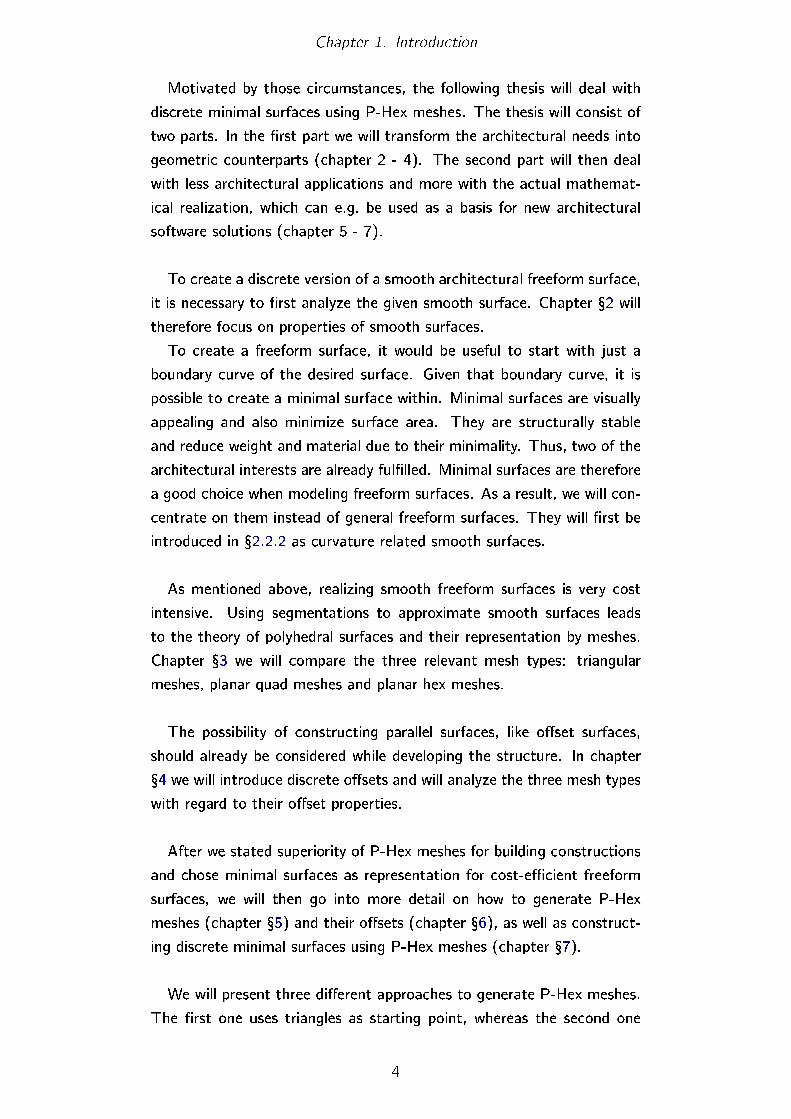
Soap �lms. Soap �lms can be used to visualize a minimal surface: They
appear, when you insert a metal curve into a basin with soap-water, such
that it is completely covered in soap-water and then carefully remove it
from the basin. The metal curve will then be the boundary curve of a
soap �lm surface. If the curve is non-planar like in Fig. 2.4, so is the
resulting minimal surface.
Figure 2.4.: Minimal surfaces as soap �lms; [3]
Those surfaces are formed due to the di�erent energies, like bending
energies, that in�uence the soap �lm. The surface displays a state of
equilibrium. If one would manually distort the surface at a point, it would
return to the equilibrium. As it turns out, the soap �lm surface also has
minimal surface area with regard to all other surfaces possible with the
given boundary curve, i.e. even slight perturbations in very small local
areas of the surface will lead to a larger surface area. Hence the name
minimal surface.
8
Chapter 2. Smooth Surfaces
Even though one might get a better feel for minimal surfaces by study-
ing the behavior of soap �lms, in general, when you want to create a
minimal surface build from other materials, you are left without the help
of e.g. bending energies or gravitation. For a given boundary curve, a sur-
face we choose will not magically transform itself into a minimal surface.
More information about the surface properties of minimal surfaces are
necessary. This relevant information is provided by the mean curvature
H (see �7.1).
From an architectural point of view smooth surfaces are just the begin-
ning of the design process. A physical realization of such surfaces would
not only be time consuming, but also extremely expensive. The smooth
surface therefore should be transformed into a discrete surface, preferably
into a polyhedral surface.
9
Chapter 3.
Polyhedral Surfaces
A discrete surface, i.e. a segmentation of a smooth surface into panels,
is represented by a so-called mesh. A mesh consists basically of a list of
vertices (or nodes), edges that connect two vertices and faces that are
bounded by edges. The actual mesh combinatorics contains the informa-
tion which vertices belong to common edges and faces [PLBW07]. For
a polyhedral surface all faces of the surface are planar.
To gain more insight into polyhedral surfaces, a closer look on di�er-
ent mesh types will be useful. From the well-known problem of tiling the
plane, we know that if only congruent copies of regular polygons were
allowed, there are only three types of tiling possible: equilateral triangles,
squares and regular hexagons. Allowing a�ne transformations leads to
other tilings with congruent copies of the three types. For a tiling of a
surface, [WLY+08] name those three types as the most promising candi-
dates, though in general, the property of the identical shape will get lost
due to the surface curvature.
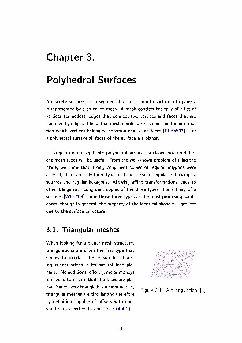
3.1. Triangular meshes
Figure 3.1.: A triangulation; [1]
When looking for a planar mesh structure,
triangulations are often the �rst type that
comes to mind. The reason for choos-
ing triangulations is its natural face pla-
narity. No additional e�ort (time or money)
is needed to ensure that the faces are pla-
nar. Since every triangle has a circumcircle,
triangular meshes are circular and therefore
by de�nition capable of o�sets with con-
stant vertex-vertex distance (see �4.4.1).
10
Chapter 3. Polyhedral Surfaces
Triangulations are well studied and can not only be found in many
building constructions, but also in renderings for the movie and games
businesses. The physical realization of a triangulation, however, is highly
ine�cient. There are high costs in manufacturing triangle faces, since it
only poorly �lls its bounding box.
Another disadvantage is the fact, that for a triangulation typically 6
faces meet in one vertex or node (less on the boundary). This so-called
high node complexity leads to higher costs when producing e.g. the needed
underlying beam structures.
A likely torsion in the nodes might also add signi�cant costs to the
manufacturing of those nodes. Torsion means the absence of a com-
mon node axis of the principal planes of incoming beams. For architec-
tural purposes as in glass-steel-constructions, triangulations compared to
e.g. quad meshes lead to less light and more weight due to the extensive
beam structure necessary.
Even though triangulations might not be the best choice for a modern
polyhedral surface, especially one with an intended physical realization, it
might still be a useful starting point for the construction of other mesh
types, like planar hex meshes (see �5.1).
3.2. Planar quad meshes (PQ meshes)
A planar quad mesh (or PQ mesh) is, as the name suggests, a quad mesh
with planar faces. The typical node complexity of a PQ mesh is 4, since 4
faces meet in one vertex. The complexity can be smaller at the boundary.
A single row of planar quad faces is called a PQ strip and is the simplest
form of a PQ mesh. Those PQ strips are the discrete analogue of smooth
developable surfaces (see �2.2.1). Complexer PQ meshes are a network
of PQ strips.
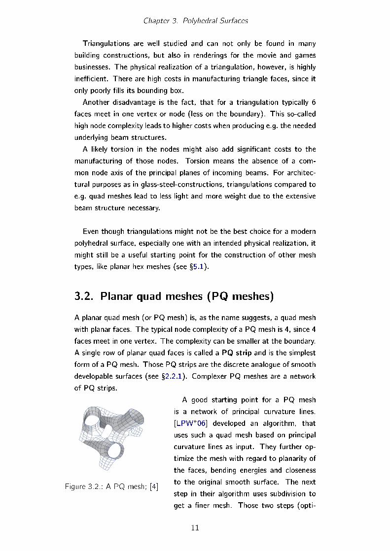
Figure 3.2.: A PQ mesh; [4]
A good starting point for a PQ mesh
is a network of principal curvature lines.
[LPW+06] developed an algorithm, that
uses such a quad mesh based on principal
curvature lines as input. They further op-
timize the mesh with regard to planarity of
the faces, bending energies and closeness
to the original smooth surface. The next
step in their algorithm uses subdivision to
get a �ner mesh. Those two steps (opti-
11
Chapter 3. Polyhedral Surfaces
mization and subdivision) alternate until the mesh ful�lls their expecta-
tions. The general PQ algorithm, however, only generates quad meshes
with planar faces. For additional properties like e.g. computing conical
meshes (see �4.4.3), the optimization step needs additional conditions
that express the conical feature.
A quad mesh can also be a good choice to create a P-Hex mesh from
(see �5.2).
3.3. Planar hex meshes (P-Hex meshes)
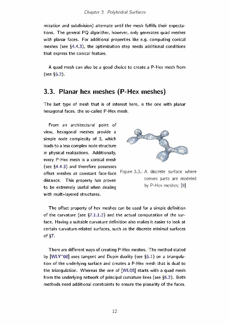
The last type of mesh that is of interest here, is the one with planar
hexagonal faces, the so-called P-Hex mesh.
Figure 3.3.: A discrete surface where
convex parts are modeled
by P-Hex meshes; [9]
From an architectural point of
view, hexagonal meshes provide a
simple node complexity of 3, which
leads to a less complex node structure
in physical realizations. Additionally,
every P-Hex mesh is a conical mesh
(see �4.4.3) and therefore possesses
o�set meshes at constant face-face
distance. This property has proven
to be extremely useful when dealing
with multi-layered structures.
The o�set property of hex meshes can be used for a simple de�nition
of the curvature (see �7.1.1.2) and the actual computation of the sur-
face. Having a suitable curvature de�nition also makes it easier to look at
certain curvature-related surfaces, such as the discrete minimal surfaces
of �7.
There are di�erent ways of creating P-Hex meshes. The method stated
by [WLY+08] uses tangent and Dupin duality (see �5.1) on a triangula-
tion of the underlying surface and creates a P-Hex mesh that is dual to
the triangulation. Whereas the one of [WL08] starts with a quad mesh
from the underlying network of principal curvature lines (see �5.2). Both
methods need additional constraints to ensure the planarity of the faces.
12
Chapter 3. Polyhedral Surfaces
Even though each method results in a P-Hex mesh, they propose a
di�erent view on hex meshes, due to their di�erent starting point (like
a triangulation or a quad mesh). Those approaches may not be equally
useful and therefore need to be carefully chosen with regard to the in-
tended outcome, i.e. additional properties that the desired P-Hex mesh
should possess. The method chosen also depends on the structure of the
underlying surface, since some methods are not able to deal with every
type of surface.
For the rest of this thesis the main mesh type focus will be on P-Hex
meshes, due to their interesting properties useful for current architec-
tural challenges. The other types and their properties might frequently
resurface, e.g. when dealing with the creation of P-Hex meshes. Chapter
�7 about discrete minimal surfaces will also use P-Hex meshes as their
polyhedral representation.
13
Chapter 4.
O�set Surfaces
In general, for a polyhedral surface it is possible to de�ne parallel meshes.
Those are meshes that possess the same combinatorics as the original
mesh and whose edges are parallel to the corresponding edges of the
original mesh. A more advanced form of a parallel mesh is the o�set
mesh: a mesh which is not only parallel to a given mesh, but also at
a constant distance to the original mesh. The distance can be de�ned
between corresponding vertices, edges or faces. This leads to three types
of o�set meshes: vertex o�sets, edge o�sets and face o�sets.
We will start by describing parallel meshes in general and then de�ne
o�set meshes and a special type of o�set meshes: the discrete Gauss
image meshes, which are meshes covering the unit sphere.
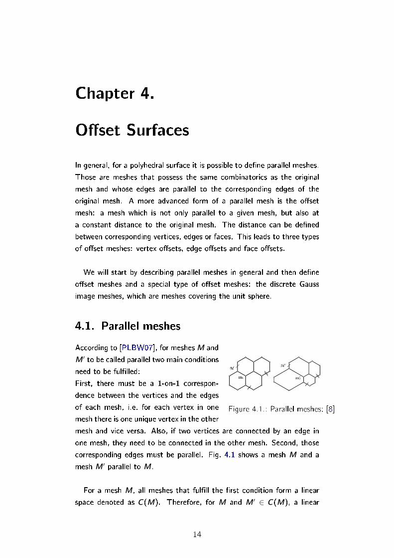
4.1. Parallel meshes
Figure 4.1.: Parallel meshes; [8]
According to [PLBW07], for meshesM and
M ′ to be called parallel two main conditions
need to be ful�lled:
First, there must be a 1-on-1 correspon-
dence between the vertices and the edges
of each mesh, i.e. for each vertex in one
mesh there is one unique vertex in the other
mesh and vice versa. Also, if two vertices are connected by an edge in
one mesh, they need to be connected in the other mesh. Second, those
corresponding edges must be parallel. Fig. 4.1 shows a mesh M and a
mesh M ′ parallel to M.
For a mesh M, all meshes that ful�ll the �rst condition form a linear
space denoted as C(M). Therefore, for M and M ′ ∈ C(M), a linear
14
Chapter 4. O�set Surfaces
combination of both can be de�ned (vertex-wise) and the resulting mesh
is again an element of C(M).
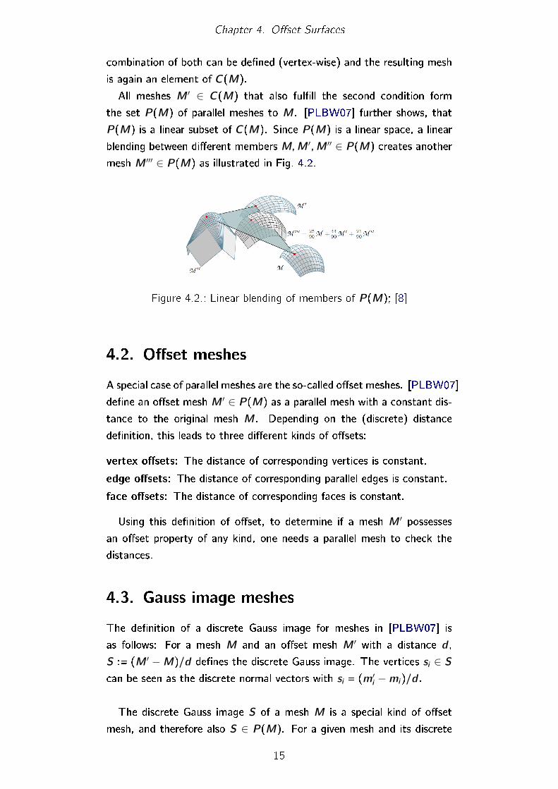
All meshes M ′ ∈ C(M) that also ful�ll the second condition form
the set P (M) of parallel meshes to M. [PLBW07] further shows, that
P (M) is a linear subset of C(M). Since P (M) is a linear space, a linear
blending between di�erent members M,M ′,M ′′ ∈ P (M) creates another
mesh M ′′′ ∈ P (M) as illustrated in Fig. 4.2.
Figure 4.2.: Linear blending of members of P (M); [8]
4.2. O�set meshes
A special case of parallel meshes are the so-called o�set meshes. [PLBW07]
de�ne an o�set mesh M ′ ∈ P (M) as a parallel mesh with a constant dis-
tance to the original mesh M. Depending on the (discrete) distance
de�nition, this leads to three di�erent kinds of o�sets:
vertex o�sets: The distance of corresponding vertices is constant.
edge o�sets: The distance of corresponding parallel edges is constant.
face o�sets: The distance of corresponding faces is constant.
Using this de�nition of o�set, to determine if a mesh M ′ possesses
an o�set property of any kind, one needs a parallel mesh to check the
distances.
4.3. Gauss image meshes
The de�nition of a discrete Gauss image for meshes in [PLBW07] is
as follows: For a mesh M and an o�set mesh M ′ with a distance d ,
S := (M ′ −M)/d de�nes the discrete Gauss image. The vertices si ∈ Scan be seen as the discrete normal vectors with si = (m′i −mi)/d .
The discrete Gauss image S of a mesh M is a special kind of o�set
mesh, and therefore also S ∈ P (M). For a given mesh and its discrete
15
Chapter 4. O�set Surfaces
Gauss image, it is easy to produce o�set surfaces for every distance d.
The discrete Gauss image represents the normal vectors of the surface,
so M + dS =M∗ with M∗ ∈ P (M) for all d.
The Gauss image mesh can be used not only to create o�sets of M,
but also for every other meshM ′ ∈ P (M). Therefore all meshes in P (M)
are of the same o�set type, since there is only one Gauss image mesh for
all of them.
4.4. O�set types and related Gauss images
Connections between the o�set type and the behavior of the Gauss image
mesh are stated by [PLBW07]. In their setting,M,M ′ are parallel meshes
with distance d and S = (M ′ −M)/d is the corresponding Gauss image
mesh. The connections are the following:
4.4.1. Vertex o�sets
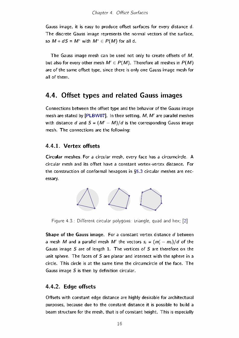
Circular meshes. For a circular mesh, every face has a circumcircle. A
circular mesh and its o�set have a constant vertex-vertex distance. For
the construction of conformal hexagons in �5.3 circular meshes are nec-
essary.
Figure 4.3.: Di�erent circular polygons: triangle, quad and hex; [2]
Shape of the Gauss image. For a constant vertex distance d between
a mesh M and a parallel mesh M ′ the vectors si = (m′i − mi)/d of the
Gauss image S are of length 1. The vertices of S are therefore on the
unit sphere. The faces of S are planar and intersect with the sphere in a
circle. This circle is at the same time the circumcircle of the face. The
Gauss image S is then by de�nition circular.
4.4.2. Edge o�sets
O�sets with constant edge distance are highly desirable for architectural
purposes, because due to the constant distance it is possible to build a
beam structure for the mesh, that is of constant height. This is especially
16
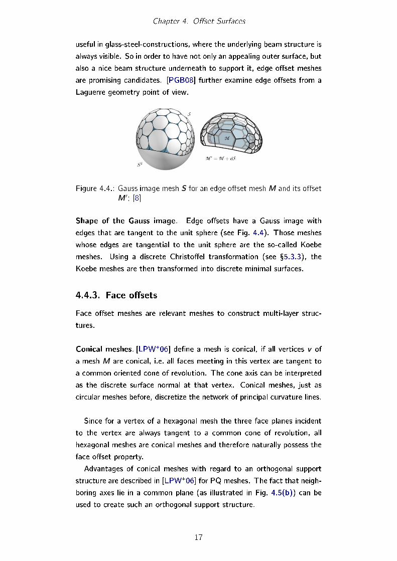
Chapter 4. O�set Surfaces
useful in glass-steel-constructions, where the underlying beam structure is
always visible. So in order to have not only an appealing outer surface, but
also a nice beam structure underneath to support it, edge o�set meshes
are promising candidates. [PGB08] further examine edge o�sets from a
Laguerre geometry point of view.
Figure 4.4.: Gauss image mesh S for an edge o�set meshM and its o�setM ′; [8]
Shape of the Gauss image. Edge o�sets have a Gauss image with
edges that are tangent to the unit sphere (see Fig. 4.4). Those meshes
whose edges are tangential to the unit sphere are the so-called Koebe
meshes. Using a discrete Christo�el transformation (see �5.3.3), the
Koebe meshes are then transformed into discrete minimal surfaces.
4.4.3. Face o�sets
Face o�set meshes are relevant meshes to construct multi-layer struc-
tures.
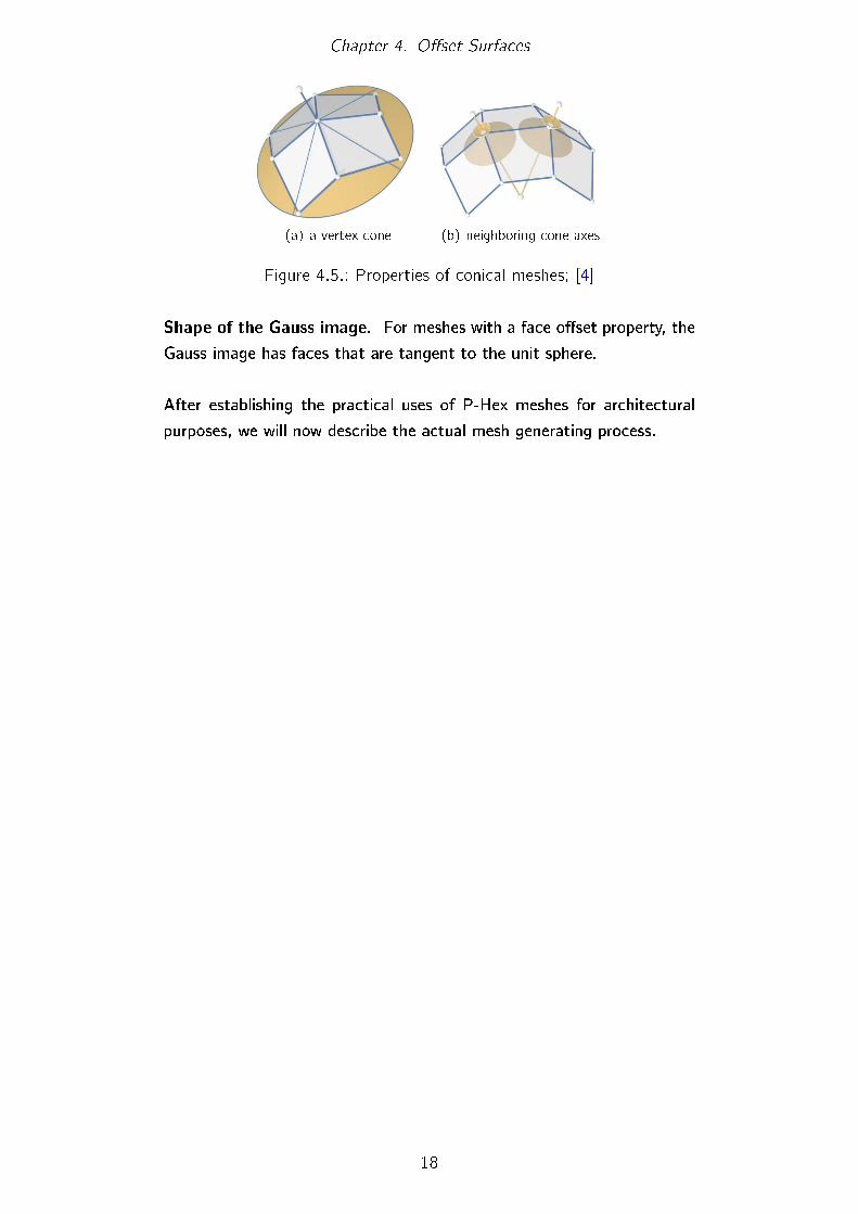
Conical meshes. [LPW+06] de�ne a mesh is conical, if all vertices v of
a mesh M are conical, i.e. all faces meeting in this vertex are tangent to
a common oriented cone of revolution. The cone axis can be interpreted
as the discrete surface normal at that vertex. Conical meshes, just as
circular meshes before, discretize the network of principal curvature lines.
Since for a vertex of a hexagonal mesh the three face planes incident
to the vertex are always tangent to a common cone of revolution, all
hexagonal meshes are conical meshes and therefore naturally possess the
face o�set property.
Advantages of conical meshes with regard to an orthogonal support
structure are described in [LPW+06] for PQ meshes. The fact that neigh-
boring axes lie in a common plane (as illustrated in Fig. 4.5(b)) can be
used to create such an orthogonal support structure.
17
Chapter 4. O�set Surfaces
(a) a vertex cone (b) neighboring cone axes
Figure 4.5.: Properties of conical meshes; [4]
Shape of the Gauss image. For meshes with a face o�set property, the
Gauss image has faces that are tangent to the unit sphere.
After establishing the practical uses of P-Hex meshes for architectural
purposes, we will now describe the actual mesh generating process.
18
Chapter 5.
P-Hex Mesh Computations
Over the last couple of years di�erent ways of creating a P-Hex mesh
have been established and used. The following overview is according to
[WL08].
Stereographic projection. The stereographic projection method starts
in a 2D setting. An extended Voronoi diagram, a so-called power diagram,
of a set of 2D points is mapped onto an ellipsoid using stereographic pro-
jection. This leads to a polyhedral surface. If the power diagram consists
of hexagonal faces, the resulting polyhedral surface will be a P-Hex mesh
approximating the ellipsoid. A huge disadvantage of this method is its re-
striction to the ellipsoid. It is therefore not possible to approximate e.g. a
hyperboloid of one sheet or a more general freeform surface instead of
the ellipsoid.
Projective duality. A di�erent approach of computing a P-Hex mesh
(proposed by [WL08]) uses a triangulation to generate the desired mesh.
The basic idea is to start by computing the dual of a given surface.
This duality maps a plane not passing through the origin, in the form
ax + by + cz + 1 = 0 in primal space, to a point (a, b, c)T in dual space.
During the next step a regular triangulation of the dual surface is com-
puted. In the �nal step, this triangulation is mapped to a P-Hex mesh
approximating the original surface.
There are, however, some problems with this approach, e.g. possi-
ble high metric distortion or singular points on the dual surfaces due to
parabolic points on the original surface. Projective duality, in general,
does not provide a one-on-one correspondence between the points of the
original surface and those of the dual surface. Additionally, this method
cannot be used to approximate a freeform surface. Even with the restric-
tion to only convex freeform surfaces, the method might still produce
19
Chapter 5. P-Hex Mesh Computations
faces with self-intersection.
Gaussian sphere. This method of computing a P-Hex mesh starts with
a freeform surface and uses the supporting function over the Gaussian
sphere of the surface. This supporting function basically is the composi-
tion of the duality and the spherical inversion with respect to S2. This
piecewise linear supporting function leads to a P-Hex mesh approximat-
ing the original freeform surface. Since this method also uses projective
duality, the same problems as for the plain projective duality method arise.
Parallel meshes. This method was developed out of the o�set theory
for mesh surfaces. It can be used to develop P-Hex meshes for simple
surfaces, like a surface path with K > 0 everywhere or K < 0 everywhere.
A major restriction of this method is, however, that a P-Hex mesh is al-
ready needed to begin with, in order to create a new one parallel to the
given mesh. Even then, this method may still produce faces with self-
intersection.
The disadvantages of these methods lead to the two basic attributes de-
sirable in a method of computing P-Hex meshes: generality and validity.
Generality in this context means, that there is no restriction as to what
type of region (elliptic, hyperbolic, parabolic) can or cannot be computed
by the method. The validity property basically ensures faces with no self-
intersection.
The following three approaches will present methods of computing a
P-Hex mesh with respect to generality and validity: In 2008 [WLY+08]
proposed a way that starts with a triangulation and develops a P-Hex
mesh using di�erent types of duality (see �5.1). In the same year [WL08]
described an additional way of getting a P-Hex mesh by starting with a
quad mesh generated from the network of conjugate curvature lines of
the underlying surface (see �5.2). The third way will be described in �5.3
and uses conformal meshes as stated by [Mue09] in 2009.
5.1. Triangle to Hex: Tangent and Dupin
duality
This approach uses of two types of dualities: tangent duality and Dupin
duality. The tangent duality describes the correspondence between a
20
Chapter 5. P-Hex Mesh Computations
triangular mesh and a P-Hex mesh. The Dupin duality will be used to
analyze the local properties of the tangent duality in more detail.
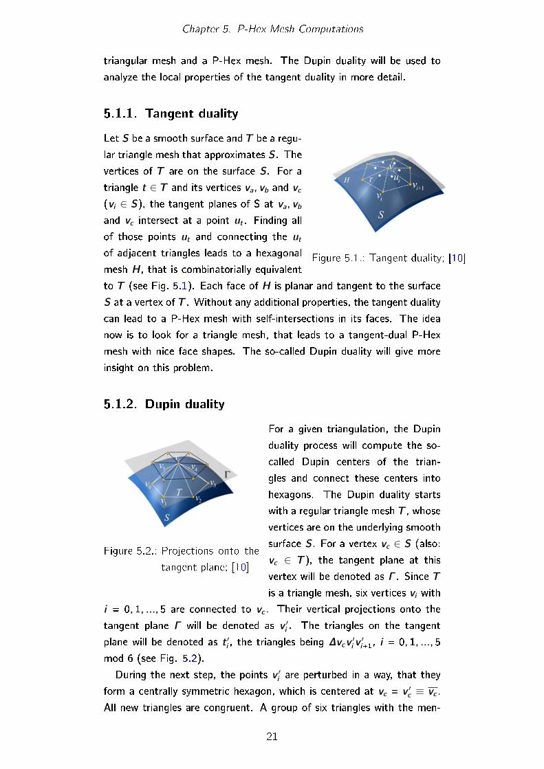
5.1.1. Tangent duality
Figure 5.1.: Tangent duality; [10]
Let S be a smooth surface and T be a regu-
lar triangle mesh that approximates S. The
vertices of T are on the surface S. For a
triangle t ∈ T and its vertices va, vb and vc
(vi ∈ S), the tangent planes of S at va, vb
and vc intersect at a point ut . Finding all
of those points ut and connecting the ut
of adjacent triangles leads to a hexagonal
mesh H, that is combinatorially equivalent
to T (see Fig. 5.1). Each face of H is planar and tangent to the surface
S at a vertex of T . Without any additional properties, the tangent duality
can lead to a P-Hex mesh with self-intersections in its faces. The idea
now is to look for a triangle mesh, that leads to a tangent-dual P-Hex
mesh with nice face shapes. The so-called Dupin duality will give more
insight on this problem.
5.1.2. Dupin duality
Figure 5.2.: Projections onto the
tangent plane; [10]
For a given triangulation, the Dupin
duality process will compute the so-
called Dupin centers of the trian-
gles and connect these centers into
hexagons. The Dupin duality starts
with a regular triangle mesh T , whose
vertices are on the underlying smooth
surface S. For a vertex vc ∈ S (also:
vc ∈ T ), the tangent plane at this
vertex will be denoted as Γ . Since T
is a triangle mesh, six vertices vi with
i = 0, 1, ..., 5 are connected to vc . Their vertical projections onto the
tangent plane Γ will be denoted as v ′i . The triangles on the tangent
plane will be denoted as t ′i , the triangles being ∆vcv′i v′i+1, i = 0, 1, ..., 5
mod 6 (see Fig. 5.2).
During the next step, the points v ′i are perturbed in a way, that they
form a centrally symmetric hexagon, which is centered at vc = v′c ≡ vc .
All new triangles are congruent. A group of six triangles with the men-
21
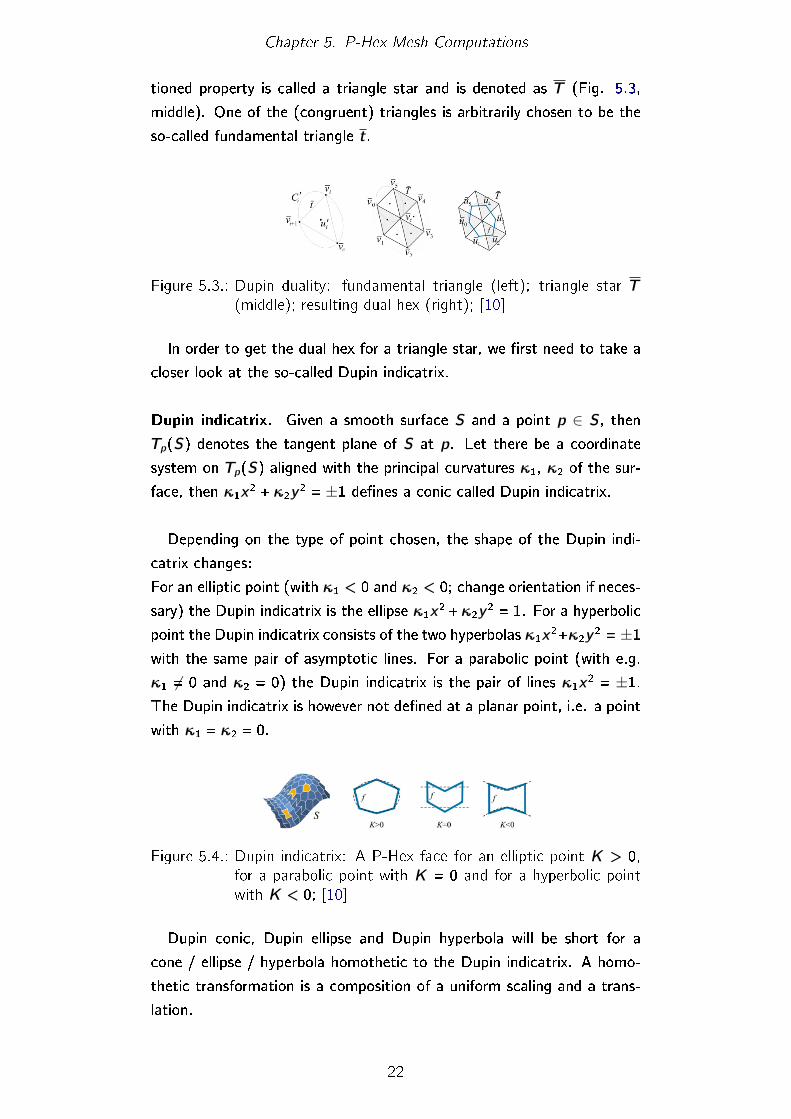
Chapter 5. P-Hex Mesh Computations
tioned property is called a triangle star and is denoted as T (Fig. 5.3,
middle). One of the (congruent) triangles is arbitrarily chosen to be the
so-called fundamental triangle t.
Figure 5.3.: Dupin duality: fundamental triangle (left); triangle star T(middle); resulting dual hex (right); [10]
In order to get the dual hex for a triangle star, we �rst need to take a
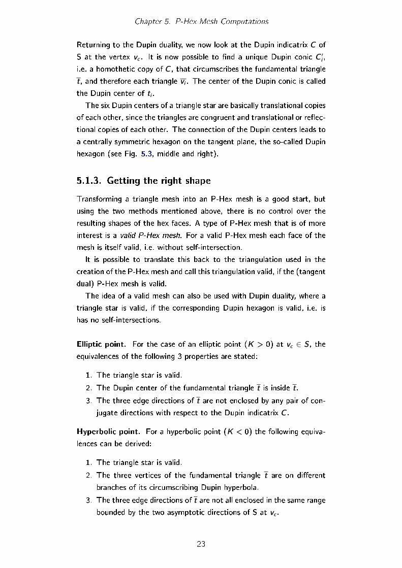
closer look at the so-called Dupin indicatrix.
Dupin indicatrix. Given a smooth surface S and a point p ∈ S, thenTp(S) denotes the tangent plane of S at p. Let there be a coordinate
system on Tp(S) aligned with the principal curvatures κ1, κ2 of the sur-
face, then κ1x2 + κ2y
2 = ±1 de�nes a conic called Dupin indicatrix.
Depending on the type of point chosen, the shape of the Dupin indi-
catrix changes:
For an elliptic point (with κ1 < 0 and κ2 < 0; change orientation if neces-
sary) the Dupin indicatrix is the ellipse κ1x2 +κ2y
2 = 1. For a hyperbolic
point the Dupin indicatrix consists of the two hyperbolas κ1x2+κ2y
2 = ±1with the same pair of asymptotic lines. For a parabolic point (with e.g.
κ1 6= 0 and κ2 = 0) the Dupin indicatrix is the pair of lines κ1x2 = ±1.
The Dupin indicatrix is however not de�ned at a planar point, i.e. a point
with κ1 = κ2 = 0.
Figure 5.4.: Dupin indicatrix: A P-Hex face for an elliptic point K > 0,for a parabolic point with K = 0 and for a hyperbolic pointwith K < 0; [10]
Dupin conic, Dupin ellipse and Dupin hyperbola will be short for a
cone / ellipse / hyperbola homothetic to the Dupin indicatrix. A homo-
thetic transformation is a composition of a uniform scaling and a trans-
lation.
22
Chapter 5. P-Hex Mesh Computations
Returning to the Dupin duality, we now look at the Dupin indicatrix C of
S at the vertex vc . It is now possible to �nd a unique Dupin conic C ′i ,
i.e. a homothetic copy of C, that circumscribes the fundamental triangle
t, and therefore each triangle vi . The center of the Dupin conic is called
the Dupin center of ti .
The six Dupin centers of a triangle star are basically translational copies
of each other, since the triangles are congruent and translational or re�ec-
tional copies of each other. The connection of the Dupin centers leads to
a centrally symmetric hexagon on the tangent plane, the so-called Dupin
hexagon (see Fig. 5.3, middle and right).
5.1.3. Getting the right shape
Transforming a triangle mesh into an P-Hex mesh is a good start, but
using the two methods mentioned above, there is no control over the
resulting shapes of the hex faces. A type of P-Hex mesh that is of more
interest is a valid P-Hex mesh. For a valid P-Hex mesh each face of the
mesh is itself valid, i.e. without self-intersection.
It is possible to translate this back to the triangulation used in the
creation of the P-Hex mesh and call this triangulation valid, if the (tangent
dual) P-Hex mesh is valid.
The idea of a valid mesh can also be used with Dupin duality, where a
triangle star is valid, if the corresponding Dupin hexagon is valid, i.e. is
has no self-intersections.
Elliptic point. For the case of an elliptic point (K > 0) at vc ∈ S, theequivalences of the following 3 properties are stated:
1. The triangle star is valid.
2. The Dupin center of the fundamental triangle t is inside t.
3. The three edge directions of t are not enclosed by any pair of con-
jugate directions with respect to the Dupin indicatrix C.
Hyperbolic point. For a hyperbolic point (K < 0) the following equiva-
lences can be derived:
1. The triangle star is valid.
2. The three vertices of the fundamental triangle t are on di�erent
branches of its circumscribing Dupin hyperbola.
3. The three edge directions of t are not all enclosed in the same range
bounded by the two asymptotic directions of S at vc .
23
Chapter 5. P-Hex Mesh Computations
The approach as described so far makes use of a valid triangulation to
produce a valid P-Hex mesh that has no self-intersections. Additionally,
one would like to have not only a valid P-Hex mesh, but also a valid P-Hex
mesh with nice face shapes.
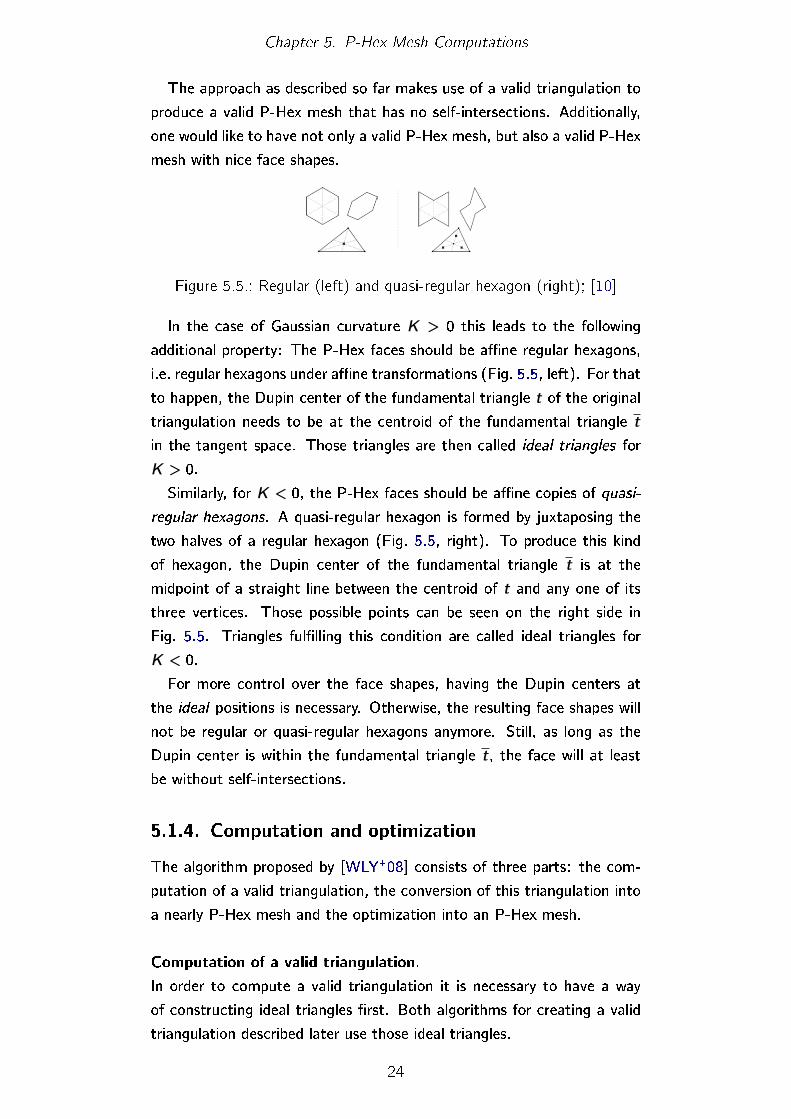
Figure 5.5.: Regular (left) and quasi-regular hexagon (right); [10]
In the case of Gaussian curvature K > 0 this leads to the following
additional property: The P-Hex faces should be a�ne regular hexagons,
i.e. regular hexagons under a�ne transformations (Fig. 5.5, left). For that
to happen, the Dupin center of the fundamental triangle t of the original
triangulation needs to be at the centroid of the fundamental triangle t
in the tangent space. Those triangles are then called ideal triangles for
K > 0.
Similarly, for K < 0, the P-Hex faces should be a�ne copies of quasi-
regular hexagons. A quasi-regular hexagon is formed by juxtaposing the
two halves of a regular hexagon (Fig. 5.5, right). To produce this kind
of hexagon, the Dupin center of the fundamental triangle t is at the
midpoint of a straight line between the centroid of t and any one of its
three vertices. Those possible points can be seen on the right side in
Fig. 5.5. Triangles ful�lling this condition are called ideal triangles for
K < 0.
For more control over the face shapes, having the Dupin centers at
the ideal positions is necessary. Otherwise, the resulting face shapes will
not be regular or quasi-regular hexagons anymore. Still, as long as the
Dupin center is within the fundamental triangle t, the face will at least
be without self-intersections.
5.1.4. Computation and optimization
The algorithm proposed by [WLY+08] consists of three parts: the com-
putation of a valid triangulation, the conversion of this triangulation into
a nearly P-Hex mesh and the optimization into an P-Hex mesh.
Computation of a valid triangulation.
In order to compute a valid triangulation it is necessary to have a way
of constructing ideal triangles �rst. Both algorithms for creating a valid
triangulation described later use those ideal triangles.
24
Chapter 5. P-Hex Mesh Computations
Since the term ideal triangle depends on the Gaussian curvature K, the
computation of an ideal triangle di�ers slightly for K > 0 and for K < 0.
We will look at the case K > 0 �rst.
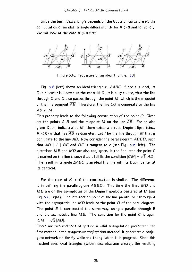
Figure 5.6.: Properties of an ideal triangle; [10]
Fig. 5.6 (left) shows an ideal triangle t: ∆ABC. Since t is ideal, its
Dupin center is located at the centroid O. It is easy to see, that the line
through C and O also passes through the point M, which is the midpoint
of the line segment AB. Therefore, the line CO is conjugate to the line
AB at M.
This property leads to the following construction of the point C: Given
are the points A,B and the midpoint M on the line AB. For an also
given Dupin indicatrix at M, there exists a unique Dupin ellipse (since
K < 0) e that has AB as diameter. Let l be the line through M that is
conjugate to the line AB. Now consider the parallelogram ABED, such
that AD ‖ l ‖ BE and DE is tangent to e (see Fig. 5.6, left). The
directions ME and MD are also conjugate. In the �nal step the point C
is marked on the line l , such that it ful�lls the condition |CM| =√3 |AD|.
The resulting triangle ∆ABC is an ideal triangle with its Dupin center at
its centroid.
For the case of K < 0 the construction is similar. The di�erence
is in de�ning the parallelogram ABED. This time the lines MD and
ME are on the asymptotes of the Dupin hyperbola centered at M (see
Fig. 5.6, right). The intersection point of the line parallel to l through A
with the asymptotic line MD leads to the point D of the parallelogram.
The point E is constructed the same way, using a parallel through B
and the asymptotic line ME. The condition for the point C is again
|CM| =√3 |AD|.
There are two methods of getting a valid triangulation presented: the
�rst method is the progressive conjugation method. It generates a conju-
gate network on-the-�y while the triangulation is in progress. Since this
method uses ideal triangles (within discretization errors), the resulting
25
Chapter 5. P-Hex Mesh Computations
P-Hex faces are nearly a�ne hexagons or quasi-regular hexagons.
The second method is the pre-speci�ed conjugation method. It adjusts
some disadvantages of the former one with regard to width and orienta-
tion of the triangle layers. Here there are two conjugate direction �elds
already speci�ed.
Creation of a nearly P-Hex mesh.
This step creates a nearly P-Hex mesh by determining and then connect-
ing the Dupin centers of the triangles. The actual algorithm consists of
4 main parts.
The �rst part is a parabolic region detection. If the triangle is in a
parabolic region, the Dupin center of that triangle is set manually to the
centroid of the triangle.
The next part determines the Dupin center of a triangle that is not
in a parabolic region. For each vertex vi in ∆v1v2v3 the other two are
projected onto the plane Γi , which is determined by vi and its normal Ni .
Next the Dupin conic Ci is computed on Γi , so that it passes through vi
and the projections of the other two vertices. The center ui of this Dupin
conic represents the Dupin center for vi .
The third part computes the Dupin center u for the triangle as the
average of the three vertex Dupin centers: u = (u1 + u2 + u3)/3.
The fourth and last part connects the Dupin centers ui of all triangles
to a hexagonal mesh H0 by using a simple mesh-duality technique. The
resulting mesh H0 is nearly planar.
Optimization to create a P-Hex mesh.
The hexagonal mesh H0 created in the step before is a good initial mesh
for the following optimization. To achieve planarity of a face, the volumes
of all 4-point subsets of vertices of the face must be zero. The term
vol(ui , uj , uk , ul) denotes the volume of a tetrahedron (ui , uj , uk , ul). The
planarity constraints for each hex-face fi is de�ned as
F (fi) :=
5∑i=0
vol2(ui , ui+1, ui+2, ui+3) = 0
with indices modulo 6. Additionally, there will be some conditions regard-
ing the distance to the input mesh and to the underlying surface. The
resulting function will be minimized using the Gauss-Newton method.
This optimization step is very fast, since the input mesh is already close
to a P-Hex mesh.
26
Chapter 5. P-Hex Mesh Computations
5.2. Quad to Hex: Conjugate curves as input
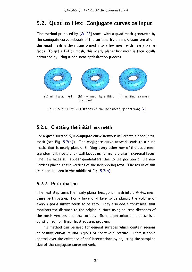
The method proposed by [WL08] starts with a quad mesh generated by
the conjugate curve network of the surface. By a simple transformation,
this quad mesh is then transformed into a hex mesh with nearly planar
faces. To get a P-Hex mesh, this nearly planar hex mesh is then locally
perturbed by using a nonlinear optimization process.
(a) initial quad mesh (b) hex mesh by shiftingquad mesh
(c) resulting hex mesh
Figure 5.7.: Di�erent stages of the hex mesh generation; [9]
5.2.1. Creating the initial hex mesh
For a given surface S, a conjugate curve network will create a good initial
mesh (see Fig. 5.7(a)). The conjugate curve network leads to a quad
mesh, that is nearly planar. Shifting every other row of the quad mesh
transforms it into a brick-wall layout using nearly planar hexagonal faces.
The new faces still appear quadrilateral due to the position of the new
vertices placed at the vertices of the neighboring rows. The result of this
step can be seen in the middle of Fig. 5.7(b).
5.2.2. Perturbation
The next step turns the nearly planar hexagonal mesh into a P-Hex mesh
using perturbation. For a hexagonal face to be planar, the volume of
every 4-point subset needs to be zero. They also add a constraint, that
monitors the distance to the original surface using squared distances of
the mesh vertices and the surface. So the perturbation process is a
constrained non-linear least squares problem.
This method can be used for general surfaces which contain regions
of positive curvature and regions of negative curvature. There is some
control over the existence of self-intersections by adjusting the sampling
size of the conjugate curve network.
27
Chapter 5. P-Hex Mesh Computations
Unfortunately, this method only produces approximately planar hex
meshes due to the optimization process.
5.3. Conformal Hex
With a view on the parallel meshes in �4.1 and more speci�c the o�set
meshes mentioned in �4.2, we know that there is a connection between
circular meshes and meshes with a vertex o�set property. In this chap-
ter about conformal hexagons, we will take a close look on the circular
property.
5.3.1. Conformal polygons
We know, that a polygon is called circular, if it possesses a circumcircle. A
type of polygon closely related to the circular polygon is the quasi-circular
polygon. It is a polygon, that is parallel to a circular polygon, i.e. they
have the same combinatorics and their edges are parallel.
To determine if a polygon is circular, the computation of the cross-
ratio (for quads) or the more general multi-ratio (for polygons with an
even number of vertices larger than 4) have proven to be very useful.
Cross-Ratio. The cross-ratio of a quadrilateral zi = (z0, z1, z2, z3) with
z0, . . . , z3 ∈ C is de�ned as
cr(z0, z1, z2, z3) =(z0 − z1)(z2 − z3)(z1 − z2)(z3 − z0)
The cross-ratio is Moebius invariant. An important connection between
the properties of the quad and the cross-ratio is the fact, that a quad is
circular if and only if the cross-ratio is real.
Multi-Ratio. An extension of the cross-ratio is the multi-ratio for poly-
gons with an even number of vertices. For a polygon zi with n vertices,
the multi-ratio can be de�ned as
q(z0, . . . , zn−1) =(z0 − z1)(z2 − z3) . . . (zn−1 − zn)(z1 − z2)(z3 − z4) . . . (zn − z0)
The multi-ratio is also Moebius invariant. If the multi-ratio is real, then
the polygon is quasi-circular, and vice versa. Similar to the cross-ratio we
get a quasi-circular polygon, if and only if the multi-ratio is real.
28
Chapter 5. P-Hex Mesh Computations
In order to compute conformal hexagons, we will now narrow our view
from arbitrary polygons (with even number of vertices) to hexagons.
Conformal hexagon. A hexagon zi = (z0, . . . , z5) is a conformal hexagon,
if and only if the cross-ratios of the two quads (z0, z1, z2, z3) and (z0, z5, z4, z3)
ful�ll
cr(z0, z1, z2, z3) = −1
2= cr(z0, z5, z4, z3).
So for a conformal hexagon, the cross-ratio of the quads is not only real,
it is always equal to −12. A conformal hexagonal mesh is then de�ned as
mesh where each face is a conformal hexagon. Next we will look at the
multi-ratio for conformal hexagons.
Multi-Ratio of a conformal hexagon. For the multi-ratio of a hexagon
we get:
q(z0, z1, z2, z3, z4, z5) =(z0 − z1)(z2 − z3)(z4 − z5)(z1 − z2)(z3 − z4)(z5 − z0)
=(z0 − z1)(z2 − z3)(z1 − z2)(z3 − z0)
·(z3 − z0)(z4 − z5)(z3 − z4)(z5 − z0)
= cr(z0, z1, z2, z3) · (−1) ·1
cr(z0, z5, z4, z3)
= −1
2· (−1) · (−
1
2)−1
= −1
So, for a conformal hexagon, both quads are circular due to their real
cross-ratio, and the hexagon itself is quasi-circular due to its real multi-
ratio.
5.3.2. Conformal surfaces
This section will describe conformal surfaces and their construction in
more detail.
Discrete conformal (hexagonal) surface. A discrete conformal (hex)
surface is a mesh that consists of conformal hexagons (i.e. hexagons
(z1, . . . , z5) with cr(z0, z1, z2, z3) = cr(z0, z5, z4, z3) = −1/2). Since the
multi-ratio of a conformal hexagon is −1, each face of a conformal surface
is quasi-circular and the surface itself possesses the vertex-o�set property.
29
Chapter 5. P-Hex Mesh Computations
A discrete conformal surface can be seen as a discrete analogue of a
smooth conformal parametrized surface.
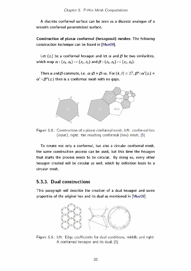
Construction of planar conformal (hexagonal) meshes. The following
construction technique can be found in [Mue09].
Let (zi) be a conformal hexagon and let α and β be two similarities,
which map α : (z4, z5) 7→ (z2, z1) and β : (z3, z4) 7→ (z1, z0).
Then α and β commute, i.e. α◦β = β◦α. For (k, l) ∈ Z2, βk◦αl(zi) =αl ◦ βk(zi) then is a conformal mesh with no gaps.
Figure 5.8.: Construction of a planar conformal mesh; left: conformal hex(input); right: the resulting conformal (hex) mesh; [5]
To create not only a conformal, but also a circular conformal mesh,
the same construction process can be used, but this time the hexagon
that starts the process needs to be circular. By doing so, every other
hexagon created will be circular as well, which by de�nition leads to a
circular mesh.
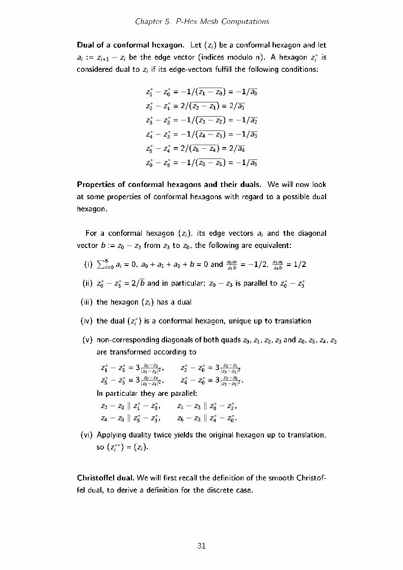
5.3.3. Dual constructions
This paragraph will describe the creation of a dual hexagon and some
properties of the original hex and its dual as mentioned in [Mue09].
Figure 5.9.: left: Edge coe�cients for dual conditions; middle and right:A conformal hexagon and its dual; [5]
30
Chapter 5. P-Hex Mesh Computations
Dual of a conformal hexagon. Let (zi) be a conformal hexagon and let
ai := zi+1 − zi be the edge vector (indices modulo n). A hexagon z∗i is
considered dual to zi if its edge-vectors ful�ll the following conditions:
z∗1 − z∗0 = −1/(z1 − z0) = −1/a0z∗2 − z∗1 = 2/(z2 − z1) = 2/a1
z∗3 − z∗2 = −1/(z3 − z2) = −1/a2z∗4 − z∗3 = −1/(z4 − z3) = −1/a3z∗5 − z∗4 = 2/(z5 − z4) = 2/a4
z∗0 − z∗5 = −1/(z0 − z5) = −1/a5
Properties of conformal hexagons and their duals. We will now look
at some properties of conformal hexagons with regard to a possible dual
hexagon.
For a conformal hexagon (zi), its edge vectors ai and the diagonal
vector b := z0 − z3 from z3 to z0, the following are equivalent:
(i)∑5
i=0 ai = 0, a0 + a1 + a2 + b = 0 and a0a2a1b
= −1/2, a3a5a4b
= 1/2
(ii) z∗0 − z∗3 = 2/b and in particular: z0 − z3 is parallel to z∗0 − z∗3
(iii) the hexagon (zi) has a dual
(iv) the dual (z∗i ) is a conformal hexagon, unique up to translation
(v) non-corresponding diagonals of both quads z0, z1, z2, z3 and z0, z5, z4, z3
are transformed according to
z∗1 − z∗3 = 3 z0−z2|z0−z2|2 , z∗2 − z∗0 = 3 z3−z1
|z3−z1|2
z∗5 − z∗3 = 3 z0−z4|z0−z4|2 , z∗4 − z∗0 = 3 z3−z5
|z3−z5|2 .
In particular they are parallel:
z2 − z0 ‖ z∗1 − z∗3 , z1 − z3 ‖ z∗0 − z∗2 ,z4 − z0 ‖ z∗5 − z∗3 , z5 − z3 ‖ z∗4 − z∗0 .
(vi) Applying duality twice yields the original hexagon up to translation,
so (z∗∗i ) = (zi).
Christo�el dual. We will �rst recall the de�nition of the smooth Christof-
fel dual, to derive a de�nition for the discrete case.
31
Chapter 5. P-Hex Mesh Computations
Smooth Christo�el dual. Let f be an isothermic parametrization. Then
the Christo�el dual f ∗, de�ned by the formulas
f ∗x =fx|fx |2
and f ∗y = −fy|fy |2
exists and is isothermic again.
The dual f ∗ is a minimal surface if and only if f is a sphere.
Discrete Christo�el dual property. Similar to the smooth case, a prop-
erty of the discrete Christo�el dual is the following: A discrete surface
is a discrete hexagonal minimal surface, if it is the dual of a conformal
mesh covering the unit sphere.
This property already states to some extent the construction process
described further in �7.2.1: During this construction process we �rst cre-
ate a conformal mesh covering the unit sphere and then construct its dual,
which by the de�nition above will then be a discrete hexagonal minimal
surface.
After dealing with the general computation of P-Hex meshes, we will now
provide information about how to gain an o�set of a P-Hex mesh.
32
Chapter 6.
O�setting P-Hex meshes
Since there are three types of o�sets possible, we will give an idea for a
creation method for each type.
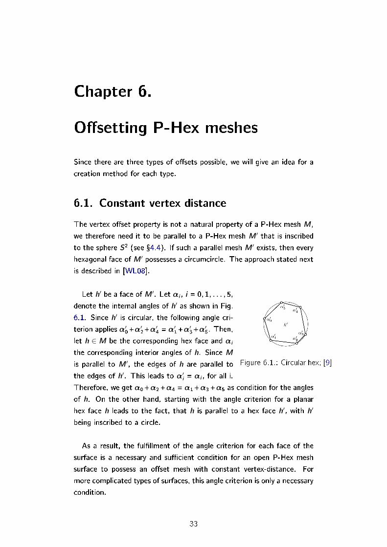
6.1. Constant vertex distance
The vertex o�set property is not a natural property of a P-Hex mesh M,
we therefore need it to be parallel to a P-Hex mesh M ′ that is inscribed
to the sphere S2 (see �4.4). If such a parallel mesh M ′ exists, then every
hexagonal face ofM ′ possesses a circumcircle. The approach stated next
is described in [WL08].
Figure 6.1.: Circular hex; [9]
Let h′ be a face of M ′. Let αi , i = 0, 1, . . . , 5,
denote the internal angles of h′ as shown in Fig.
6.1. Since h′ is circular, the following angle cri-
terion applies α′0+α′2+α
′4 = α
′1+α
′3+α
′5. Then,
let h ∈M be the corresponding hex face and αi
the corresponding interior angles of h. Since M
is parallel to M ′, the edges of h are parallel to
the edges of h′. This leads to α′i = αi , for all i.
Therefore, we get α0+α2+α4 = α1+α3+α5 as condition for the angles
of h. On the other hand, starting with the angle criterion for a planar
hex face h leads to the fact, that h is parallel to a hex face h′, with h′
being inscribed to a circle.
As a result, the ful�llment of the angle criterion for each face of the
surface is a necessary and su�cient condition for an open P-Hex mesh
surface to possess an o�set mesh with constant vertex-distance. For
more complicated types of surfaces, this angle criterion is only a necessary
condition.
33
Chapter 6. O�setting P-Hex meshes
6.2. Constant edge distance
The following method of creating a hexagonal edge o�set mesh (EO
mesh) was proposed by [PLBW07]. It uses a Koebe polyhedron as start-
ing point.
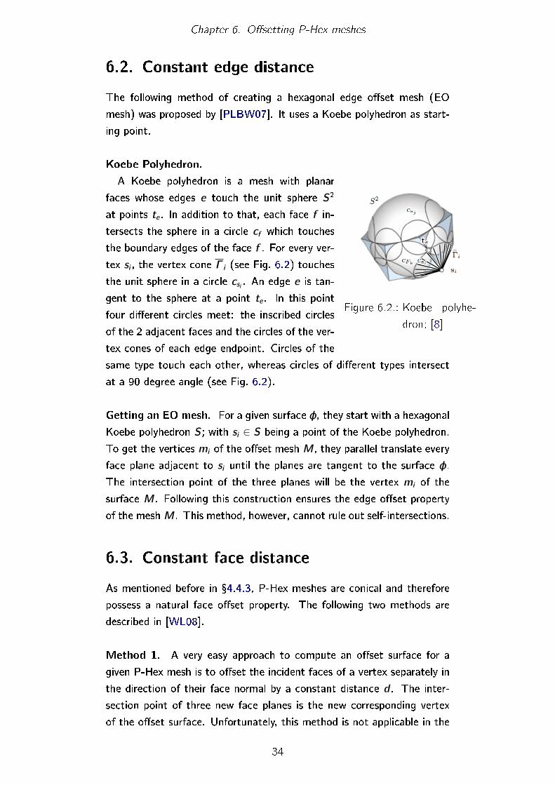
Koebe Polyhedron.
Figure 6.2.: Koebe polyhe-
dron; [8]
A Koebe polyhedron is a mesh with planar
faces whose edges e touch the unit sphere S2
at points te . In addition to that, each face f in-
tersects the sphere in a circle cf which touches
the boundary edges of the face f . For every ver-
tex si , the vertex cone Γ i (see Fig. 6.2) touches
the unit sphere in a circle csi . An edge e is tan-
gent to the sphere at a point te . In this point
four di�erent circles meet: the inscribed circles
of the 2 adjacent faces and the circles of the ver-
tex cones of each edge endpoint. Circles of the
same type touch each other, whereas circles of di�erent types intersect
at a 90 degree angle (see Fig. 6.2).
Getting an EO mesh. For a given surface φ, they start with a hexagonal
Koebe polyhedron S; with si ∈ S being a point of the Koebe polyhedron.
To get the vertices mi of the o�set mesh M, they parallel translate every
face plane adjacent to si until the planes are tangent to the surface φ.
The intersection point of the three planes will be the vertex mi of the
surface M. Following this construction ensures the edge o�set property
of the meshM. This method, however, cannot rule out self-intersections.
6.3. Constant face distance
As mentioned before in �4.4.3, P-Hex meshes are conical and therefore
possess a natural face o�set property. The following two methods are
described in [WL08].
Method 1. A very easy approach to compute an o�set surface for a
given P-Hex mesh is to o�set the incident faces of a vertex separately in
the direction of their face normal by a constant distance d . The inter-
section point of three new face planes is the new corresponding vertex
of the o�set surface. Unfortunately, this method is not applicable in the
34
Chapter 6. O�setting P-Hex meshes
case of three co-planar faces and will be numerically unstable when they
are nearly co-planar.
Method 2. This next method will take the interior angles of the faces at a
vertex of the mesh into consideration when computing the vertex normal.
Let M be a P-Hex mesh, v ∈ M a vertex and let fi with i = 0, 1, 2 be
the faces incident at v . The corresponding vertex of the o�set surface
(at distance d) will be denoted as vd (with vd ∈Md). Let Ni be the unit
normal vectors of the faces fi . Let θi be the internal angle of fi at v . The
vertex normal of v will then be computed as follows:
Nv =
2∑i=0
(tanβi + tan γi)Ni
where βi =12(θi + θi+1 − θi−1) and γi =
12(θi + θi−1 − θi+1), i = 0, 1, 2
mod (3). With this formula, the vertex vd can be determined by inter-
secting the line p(t) = v + tNv with any of the o�set planes of the faces.
After we established the discrete o�set capabilities of P-Hex meshes, we
can now use an analogue of smooth curvature de�nitions from o�set
properties to de�ne discrete curvatures and therefore discrete minimal
surfaces.
35
Chapter 7.
Discrete Minimal Surfaces
Smooth minimal surfaces are de�ned as surfaces with vanishing mean
curvature. If we want to de�ne a similar version for the discrete case,
we �rst need to de�ne the curvatures of a discrete surface. The idea
of transforming the smooth curvature de�nitions into discrete ones is a
promising approach, but it is important to realize, that the equivalence of
the smooth curvature de�nitions might not translate accordingly. There-
fore a discrete realization of a smooth minimal surface might not be
minimal, depending on the mesh and the curvature de�nition used for
the realization. It is therefore a goal of the discrete minimal surface the-
ory, to �nd representations that ful�ll more than just one de�nition; see
[PBCW07].
First we will present de�nitions of discrete curvatures and discrete min-
imal surfaces, which will not be restricted to any speci�c mesh or o�-
set type. In the second part, we will concentrate on di�erent creation
methods for discrete minimal surfaces based on P-Hex meshes.
7.1. Vanishing mean curvature
An important value of a surface with regard to minimal surfaces is the
mean curvature. This section will broaden the basic de�nitions necessary
for the smooth case as stated in �2.1 and then demonstrate, how to
translate those into the discrete case. Two di�erent approaches for the
discrete curvature de�nitions will be described.
36
Chapter 7. Discrete Minimal Surfaces
7.1.1. Curvature
7.1.1.1. Smooth case
The following de�nitions for the smooth case are translated versions of
the ones in [Küh05].
Surface patch. Let U ⊂ R2 be open. A parametrized surface patch is
an immersion of the kind f : U → R3, (u1, u2) 7→ f (u1, u2). The map f is
called parametrization, the elements of U are called parameter and their
images are called points or vertices.
Tangent plane. The map f is an immersion. The vectors ∂f∂u
and ∂f∂v
are therefore linearly independent and span the so-called tangent plane
Tuf for u ∈ U. Its orthogonal complement is the one-dimensional normal
space.
First fundamental form. The �rst fundamental form I of a surface
patch is de�ned as I(X, Y ) := 〈X, Y 〉 with X, Y ∈ Tuf .
Gauss map. Let S2 be the unit sphere. Then, for a surface patch
f : U → R3, the Gauss map ν : U → S2 is de�ned as
ν(u1, u2) :=
∂f∂u1× ∂f
∂u2∥∥∥ ∂f∂u1× ∂f
∂u2
∥∥∥ν(u1, u2) represents the unit normal vector placed at the origin of the
surrounding space.
Weingarten map. The map L := −Dν ◦ (Df )−1, with its point-wise
de�nition Lu := −(Dν|u) ◦ (Df |u)−1 : Tuf → Tuf is called Weingarten
map. For every parameter u, this is a linear endomorphism of the tangent
plane in f (u). The map L is independent of the parametrization and is
self-adjoint with regard to the �rst fundamental form I.
Second fundamental form. Let f : U → R3 and ν : U → S2, L be the
Weingarten map and X, Y tangent vectors. Then II(X, Y ) := I(LX, Y )
is called the second fundamental form.
37
Chapter 7. Discrete Minimal Surfaces
Principal curvatures. Let X ∈ Tuf be a unit normal vector. X is called
principal curvature direction of f, if one of the two equivalent conditions
is ful�lled:
(i) II(X,X) has a stationary value for all X with I(X,X) = 1
(ii) X is eigenvector of L. The eigenvalue λ with (LX = λX) is called
principal curvature.
Gauss and mean curvature. Using the principal curvature de�nition we
stated above, we get the following de�nitions:
(i) The determinate K = det(L) = κ1 · κ2 is the Gauss curvature of f.(ii) The value H = 1
2tr(L) = 1
2(κ1 + κ2) is the mean curvature of f.
Those curvatures also appear within a formula that describes the varia-
tion of surface area when passing from a surface φ to an o�set surface φd .
A point x ∈ φ is moved to x+dn(x), where n is the �eld of unit normal
vectors. Then, using Steiner's formula, the change in surface area can
be described as
area(φd) =
∫φ
(1− 2dH(x) + d2K(x))dx,
where K and H denote the Gauss and mean curvature, respectively.
7.1.1.2. Discrete case
Contrary to the smooth case, �nding a suitable curvature de�nition for a
mesh is not as easy. Depending on the chosen part of the mesh (e.g. edges
or faces), di�erent de�nitions of curvature are possible. We will �rst recall
the de�nition of the Gauss image mesh and then de�ne the mixed area of
two parallel polygon. Using those, we will derive the discrete curvatures
related to faces and to edges.
Gauss image mesh and discrete surface variation. The Gauss im-
age mesh de�ned in �4.3 can be interpreted as the discrete analogue of
the smooth Gauss map. Similar to the smooth case, for a mesh M one
can de�ne an o�set mesh Md = M + dS, where the Gauss image mesh
σ(M) = S provides the normal vectors.
38
Chapter 7. Discrete Minimal Surfaces
Using the same construction for the variation of surface area as for a
smooth surface, [PLBW07] propose a similar de�nition for a meshM and
its o�set Md :
area(Md) =∑F
(1− 2dHF + d2KF )area(F ), F: faces of M .
Within this formula, HF denotes the discrete mean curvature and KF the
discrete Gauss curvature of a face F . To describe HF and KF using face
properties, we will now introduce the so-called mixed area of two parallel
polygons, as described by [BPW09].
Mixed area of parallel polygons. For a polygon P = (p0, . . . , pn−1) the
oriented area can be described using Leibniz' sector formula. The area
then is computed as
area(P ) =1
2
∑0≤i<n
det(pi , pi+1)
with indices modulo n. The so de�ned area(P ) is a quadratic form and
its associated symmetric bilinear form area(P,Q) is de�ned as
area(λP + µQ) = λ2area(P ) + 2λµ · area(P,Q) + µ2area(Q).
Using this de�nition for a face F of the mesh M and its corresponding
face F d ∈Md of the o�set mesh at distance d, we get:
area(F d) = area(F + dσ(F ))
= area(F ) + 2d · area(F, σ(F )) + d2area(σ(F ))
The term area(F, σ(F )) is called mixed area of F and σ(F ).
Face curvatures. Comparing the formula for the area of an o�set face
using mixed areas with the one for the variation of surface area, we get
the following connection between the discrete curvatures and the mixed
area of a face and its o�set face:
area(F d) = (1− 2dHf + d2KF ) · area(F )
= area(F ) + 2d · area(F, σ(F )) + d2area(σ(F ))
= (1 + 2darea(F, σ(F ))
area(F )+ d2area(σ(F ))
area(F )) · area(F )
39

Chapter 7. Discrete Minimal Surfaces
This leads to the following discrete curvature de�nitions:
HF = −area(F, σ(F ))
area(F )
KF =area(σ(F ))
area(F )
The de�nitions for the discrete Gauss and mean curvature are similar to
the smooth case. Not only is the Gauss curvature de�ned as the quotient
of areas of the Gauss image and the original surface, but also principal
curvatures can be de�ned for most faces, such that HF = (κ1,F +κ2,F )/2
and KF = κ1,F · κ2,F (see �7.1.1.1).
Edge curvatures. A di�erent approach is the one proposed by [BPW09],
where the curvature terms are not associated with the faces of the mesh,
but with the edges. Hence the name.
In the edge curvature de�nition the edge vectors are interpreted as
tangent vectors. Let m be a discrete surface with combinatorics (V,E,F).
For an edge (i , j) ∈ E the edge mimj of the mesh is parallel to its corre-
sponding edge sisj of the Gauss image mesh. The edge curvature κe for
an edge e = (i , j) ∈ E is then de�ned as: sj − si = κi j(mj −mi).
For a quadrilateral mesh, it is nonetheless possible to determine the
curvatures associated with the face, i.e. the Gauss and the mean curva-
ture. As stated by [BPW09], the face curvatures can be computed as
follows:
HF =κ01κ23 − κ12κ30
κ01 + κ23 − κ12 − κ30KF =
κ01κ12κ23κ30κ01 + κ23 − κ12 − κ30
(1
κ12+
1
κ30−
1
κ01−
1
κ23)
7.1.2. Zero mean curvature
In the smooth setting, a minimal surface can be de�ned as follows:
Necessary condition for a smooth minimal surface. Let f : U → R3
be a surface patch, U ⊂ R2 open, U compact with boundary ∂U. For the
surface area of f to be smaller than or equal to the surface area of all
normal variations of the type
fε : U → R3 with fε|∂U = f |∂U ′
40

Chapter 7. Discrete Minimal Surfaces
a necessary condition is a vanishing mean curvature H on U, everywhere;
[Küh05].
Using the smooth case de�nition as a model, the de�nition for a dis-
crete minimal surface would be to have zero (discrete) mean curvature
everywhere.
In the approach of [PLBW07], zero mean curvature everywhere is
equivalent to vanishing mixed area for all faces of the mesh and their
corresponding faces of the o�set mesh. Figure 7.1 shows an example of
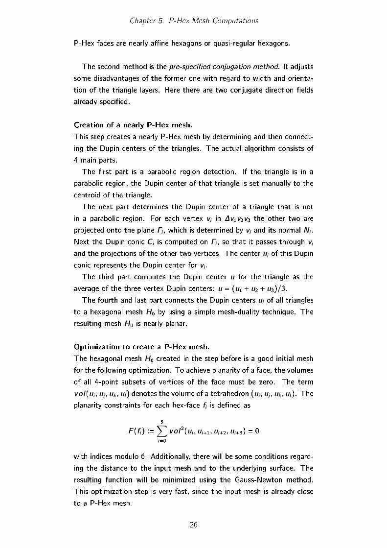
two parallel hexagons with vanishing mixed area.
Figure 7.1.: Parallel hexagons with vanishing mixed area; [6]
The edge curvature approach would state a condition for the edges to
ensure zero mean curvature. Since the edge curvature approach is used
for quadrilateral meshes and our main focus is on hexagonal meshes, we
will not go into more detail about edge curvatures.
7.2. Creating discrete hexagonal minimal
surfaces
We will describe two di�erent ways of creating a hexagonal minimal sur-
face. The �rst one is restricted to conformal hexagonal meshes, whereas
the second one uses non-convex hexagonal meshes.
7.2.1. Hexagonal Gauss image via conformal hexagons
The method for creating discrete minimal surfaces using conformal hexagons
was established by [Mue09]. A discrete (hexagonal) minimal surface is
de�ned to be the dual of a conformal mesh covering the unit sphere. The
process starts with a conformal parametrization of a part of the plane
and uses stereographic projection to create the Gauss image mesh. The
Christo�el dual from this newfound Gauss image is then, by de�nition, a
discrete hexagonal minimal surface.
41

Chapter 7. Discrete Minimal Surfaces
The resulting discrete minimal surfaces of this method are dependent
on the used conformal parametrization and do not approximate an under-
lying smooth surface.
[Mue09] explains through di�erent examples the relation between the
input hex mesh and the resulting discrete hexagonal minimal surface. We
will now describe the basic setting that is necessary for the following
examples: All examples described here start with a circular hexagonal
conformal mesh in C and use the approach described above to retrieve a
discrete hexagonal minimal surface.
The creation of the conformal hexagonal mesh is done as described in
�5.3.2. After that, a point z ∈ C is chosen, such that α(z) 6= z 6= β(z).The mesh αm−n ◦β2n(z) with (m, n) ∈ Z2 is called a derived quad mesh.
This quad mesh represents a discrete parametrization of the original con-
formal hexagonal mesh.
Three di�erent cases regarding the similarities can be distinguished:
(i) Both similarities are translations.
(ii) α is a rotation and β is a dilation with the same �xed point.
(iii) Both, α and β are similarities with the same �xed point, but di�erent
from a pure translation, rotation or dilation.
The derived quad mesh (with (m, n) ∈ Z2) can be of the following
forms depending on the similarity case:
(i) m + in ; (ii) ea(m+in) ; (iii) e(a+ib)(m+in).
Each case number relates to the appropriate case of similarities. Having
those three cases, the meshes discretize the following mappings: z 7→ z ,
z 7→ eaz and z 7→ e(a+ib)z . Next we will give an example for each type.
Case 1: z 7→ z .
In this case the conformal hexagonal mesh consists of regular hexagons.
The resulting discrete minimal surface via Christo�el duality of the Gauss
image is the discrete Enneper's surface. Fig. 7.2 shows the regular hexag-
onal mesh on the left. The middle image represents the Gauss image
mesh created by stereographic projection. And the right image displays
the resulting discrete hexagonal minimal surface.
42

Chapter 7. Discrete Minimal Surfaces
Figure 7.2.: Case 1: the initial mesh (left), the corresponding Gauss im-age (middle) and the resulting discrete Enneper's surface(right); [5]
Case 2: z 7→ eaz .
In case 2 the hexagonal mesh in the beginning is not created from a regular
hexagon anymore, but a symmetric hexagon that is Moebius equivalent
to a regular hexagon. Applying the similarities of this case to the hexagon
leads to a circular conformal mesh with rotational symmetry. This time,
the resulting discrete minimal surface is a discrete catenoid. Fig. 7.3
shows the di�erent stages of this case.
Figure 7.3.: Case 2: the initial mesh (left), the corresponding Gauss im-age (middle) and the resulting discrete catenoid (right); [5]
Case 3: z 7→ e(a+ib)z .
For the last case, the starting hexagon can be of arbitrary shape, which
is not regular but Moebius equivalent to a regular hexagon. Applying the
appropriate similarities can lead to di�erent discrete minimal surfaces,
depending on the choice of a. For a ∈ R, it leads again to a catenoid.
For a ∈ iR this process generates a helicoid. For the helicoid shown in
Fig. 7.5 the choice is a = i .
Figure 7.4.: Case 3: the initial mesh (left) and the corresponding Gaussimage (right); [5]
43
Chapter 7. Discrete Minimal Surfaces
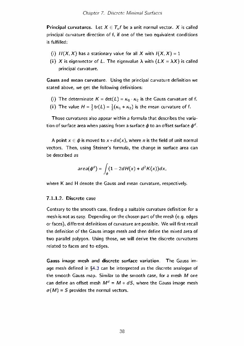
Figure 7.5.: Case 3: the resulting discrete helicoid; [5]
7.2.2. Hexagonal Gauss image via spacial hex centers
The following method to create a discrete hexagonal minimal surface
stated by [MW00] also uses Christo�el duality.
Christo�el duality. The Christo�el duality for this context is described in
[MW00], and states that the faces of a polyhedral surface and its parallel
Gauss image have vanishing mixed area. They state, that for two par-
allel quadrilaterals to have vanishing mixed area, the non-corresponding
diagonals must also be parallel. They later use this proposition also for
hexagons, by splitting a hexagon into two quads and applying the propo-
sition for each quad separately.
The method. Starting with an isothermic curvature line parametrization
of a smooth minimal surface (for Fig. 7.6 and Fig. 7.7 this would be a
smooth Enneper's surface), the parameter domain will be tiled with non-
convex hexagons. Mapping those hexagons onto the surface using the
given parametrization leads to a hex mesh with non-planar faces inscribed
to the surface. The centers of the planar hexagons are determined and
then mapped using the parametrization, which leads to points that can
be considered as the centers of the spacial hexagons.
During the next step, we construct the Gauss image using those spacial
hex centers. For each one, the tangent plane to the smooth surface is be
parallel translated to touch the unit sphere. The vertices of the discrete
Gauss image are represented by the intersection points of the di�erent
tangent planes. This procedure leads to a face o�set property of the
resulting mesh.
To gain a vertex or edge o�set property, this process changes, since
then the vertices or edges, respectively, need to be inscribed (for a vertex
o�set) or tangent (for an edge o�set) to the sphere.
44
Chapter 7. Discrete Minimal Surfaces
By using optimization during the �nal step, the non-planar hex mesh
is transformed into the Christo�el dual of the discrete Gauss image. The
optimization ensures for one, that corresponding faces of the Gauss image
and the new mesh have vanishing mixed areas. It also ensures parallelity
of corresponding edges. The optimization process itself is done by mini-
mizing a quadratic function.
(a) Gauss image Σ1 (b) Discrete Enneper's surfaceΦ1
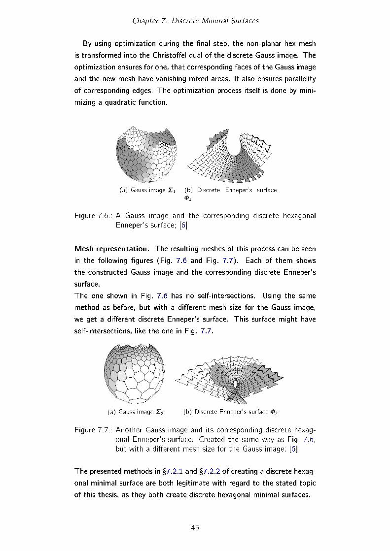
Figure 7.6.: A Gauss image and the corresponding discrete hexagonalEnneper's surface; [6]
Mesh representation. The resulting meshes of this process can be seen
in the following �gures (Fig. 7.6 and Fig. 7.7). Each of them shows
the constructed Gauss image and the corresponding discrete Enneper's
surface.
The one shown in Fig. 7.6 has no self-intersections. Using the same
method as before, but with a di�erent mesh size for the Gauss image,
we get a di�erent discrete Enneper's surface. This surface might have
self-intersections, like the one in Fig. 7.7.
(a) Gauss image Σ2 (b) Discrete Enneper's surface Φ2
Figure 7.7.: Another Gauss image and its corresponding discrete hexag-onal Enneper's surface. Created the same way as Fig. 7.6,but with a di�erent mesh size for the Gauss image; [6]
The presented methods in �7.2.1 and �7.2.2 of creating a discrete hexag-
onal minimal surface are both legitimate with regard to the stated topic
of this thesis, as they both create discrete hexagonal minimal surfaces.
45

Chapter 7. Discrete Minimal Surfaces
The �rst method only works with three types of meshes, which lead to
3 pre-de�ned minimal surface types: discrete Enneper's surfaces, discrete
catenoids or discrete helicoids. All three surface types are not particularly
useful for architectural purposes. The second method, however, is ca-
pable of approximating any kind of smooth minimal surface. It therefore
provides more �exibility for an architectural design using minimal surfaces.
46
Chapter 8.
Conclusion
In the last chapter, we have demonstrated a process of developing a dis-
crete hexagonal minimal surface that approximates a given minimal sur-
face. It is therefore possible to start an architectural design by creating
a suitable boundary curve and then compute a matching smooth minimal
surface for it. Applying the method described in �7.2.2 then produces an
approximation of the given surface by a discrete minimal surface using
P-Hex meshes.
Those resulting surfaces ful�ll most of the main interests of an archi-
tectural design process stated in the introduction: They provide a useful
segmentation into planar parts which reduces production costs. In addi-
tion to that, they are equipped with a natural o�set property, which can
be used to construct multi-layered surfaces with constant face distances.
Due to having the smallest node complexity, their supporting beam struc-
ture is less complicated to realize than for other mesh types. The use
of minimal surfaces leads to a reduced amount of construction materials
and is therefore very cost-e�cient.
So far, only a few of already existing architectural problems have been
dealt with using geometry. It is, e.g. di�cult to construct a discrete
minimal surface without a given boundary curve. Also designs with singu-
larities still pose problems for some of the existing computation methods.
In addition, more architectural parameters need to be incorporated during
the creation of polyhedral surfaces, like for instance issues regarding the
statics or the stability of the resulting surface.
With the increasing demands from new and more challenging architec-
tural designs, even more problems will arise and will further the mathe-
matical research.
47

Chapter 8. Conclusion
The existing results and the problems stated are still on a theoretical
level. To make those results more accessible and applicable for architects,
a software implementation is required.
As a consequence, the interface between the three sciences math, ar-
chitecture and computer science will gain momentum. Those new de-
velopments call for a more interdisciplinary approach currently underrep-
resented in existing research programs. To ensure a rich knowledge ex-
change, the need for people with a background in all three sciences is
increasing.
48
Appendix A.
Zusammenfassung
Entwicklungen der modernen Architektur weg von herkömmlichen For-
men und Verfahren hin zu einem deutlich freieren Gestalten sogenan-
nter Freiform�ächen haben ein neues Anwendungsfeld in der Mathematik,
spezieller der Geometrie, ins Leben gerufen. Das Feld der Architektur-
Geometrie beschäftigt sich mit geometrischen Konstrukten und Proble-
men, die mit der Herstellung von Freiform�ächen zusammenhängen.
Im Rahmen dieser Diplomarbeit habe ich mich mit der diskreten Real-
isierung von glatten Flächen, insbesondere von Minimal�ächen, beschäftigt
und ihre Nützlichkeit im Zusammenhang mit architektonischen Freiform-
�ächen dargestellt. Dazu wurden im ersten Teil der Arbeit notwendige
Begri�e und Eigenschaften wie z. B. Krümmung oder O�sets von Flächen
erläutert. Im zweiten Teil wurden dann explizit Verfahren beschrieben, mit
denen man die gewünschten Formen mathematisch erzeugen kann.
Kapitel �2 beschreibt grundlegende Eigenschaften glatter Flächen und
stellt Minimal�ächen als Flächen mit verschwindender mittlerer Krüm-
mung vor. Minimal�ächen gelten als harmonisch und visuell ansprechend.
Da sich für eine beliebige geschlossene Randkurve immer eine passende
Minimal�äche �nden lässt, eignen sie sich als Grundlage für ästhetische
Freiform�ächen in der Architektur, da man bereits aus einer Randkurve
eine ansprechende Fläche erzeugen kann.
Eine physikalische Umsetzung dieser glatten Freiform�ächen ist häu-
�g mit sehr groÿem Aufwand und hohen Kosten verbunden. Nutzt man
die glatte Freiform�äche jedoch als Ausgangspunkt für eine Zerlegung in
kostengünstigere Teile, so lassen sich damit ähnlich ansprechende For-
men realisieren. Kapitel �3 beschreibt daher unterschiedliche Netzstruk-
turen (sogenannte Meshes) für eine solche Zerlegung und nennt Vor- und
49
Appendix A. Zusammenfassung
Nachteile der unterschiedlichen Typen.
Um mehrschichtige Konstruktionen ermöglichen zu können, werden in
Kapitel �4 parallele Meshes und insbesondere O�sets betrachtet. Waren
Flächen-O�sets im glatten Fall noch eindeutig, so ergeben sich für den
diskreten Fall unterschiedliche Arten auf Grund von drei verschiedenen
Abstandsbegri�en. Der Abstand im diskreten Fall kann zwischen Knoten,
zwischen Kanten oder zwischen Flächen bestimmt werden. Daraus ergeben
sich auch die entsprechenden O�set-Typen: O�sets mit konstantem Ab-
stand zwischen den Knoten, den Kanten oder den Flächen.
Das Kapitel �5 beschreibt die Erzeugung von P-Hex Meshes auf drei
unterschiedlichen Wegen. Obwohl P-Hex Meshes auf Grund ihres Aufbaus
bereits eine Flächen-O�set-Eigenschaft besitzen, ist es auch möglich die
anderen beiden O�set-Typen mit P-Hex Meshes zu realisieren. Kapitel
�6 beschreibt die Herstellung aller drei O�set-Typen für P-Hex Meshes.
Im Kapitel �7 werden die bis dahin entwickelten Verfahren genutzt und
erweitert, um diskrete Minimal�ächen für P-Hex Meshes zu erzeugen.
Eine diskrete Minimal�äche wurde analog zum glatten Fall als eine Fläche
mit verschwindender mittlerer Krümmung de�niert. Daher bedurfte es
zunächst einer De�nition der diskreten mittleren Krümmung und damit
auch eines allgemeinen Krümmungsbegri�s für den diskreten Fall.
Im weiteren Verlauf des Kapitels wurden dann zwei unterschiedliche
Verfahren genannt, um diskrete Minimal�ächen mit P-Hex Meshes zu
erzeugen. Das erste Verfahren benötigt zwar keine glatte Minimal�äche,
schränkt jedoch die resultierenden diskreten Minimal�ächen auf Variatio-
nen der Enneper Fläche, des Katenoids und des Helicoids ein. Das zweite
Verfahren ermöglicht hingegen die Annährung einer beliebig vorgegebe-
nen glatten Minimal�äche. Im Zusammenhang mit Architektur ist daher
das zweite Verfahren besser geeignet.
Die in dieser Arbeit beschriebenen Erfolge in der Zusammenarbeit zwis-
chen Architektur und Mathematik sind bisher häu�g noch auf theoretis-
che Ebene. Für einen stärkeren praktischen Nutzen aus dieser Forschung
bedarf es einer geschickten Umsetzung der Theorie in eine für den Ar-
chitekten leicht nutzbare Form. Das Gebiet der Architektur-Geometrie
bietet daher nicht nur für Architekten und Mathematiker Potential, son-
dern auch für Informatiker, die an einer praktikablen Software-Umsetzung
maÿgeblich beteiligt sein werden.
50
Appendix B.
References
B.1. Books and Articles
[BPW09] Alexander I. Bobenko, Helmut Pottmann, and Johannes Wall-
ner. A curvature theory for discrete surfaces based on mesh
parallelity. Mathematische Annalen, 348(1):1�24, December
2009. 39, 40
[Küh05] Wolfgang Kühnel. Di�erential Geometrie - Kurven, Flächen,
Mannigfaltigkeiten. Friedr. Vieweg & Sohn Verlag / GWV
Fachverlage GmbH, Wiesbaden, 2005. 37, 41
[LPW+06] Yang Liu, Helmut Pottmann, Johannes Wallner, Yong-Liang
Yang, and Wenping Wang. Geometric modeling with coni-
cal meshes and developablesurfaces. ACM Trans. Graphics,
25(3):681�689, 2006. Proc. SIGGRAPH. 11, 17
[Mue09] Christian Mueller. Conformal hexagonal meshes. Geom. Ded-
icata (2011), pages 1�22, 2009. 3, 20, 30, 41, 42
[MW00] Christian Müller and Johannes Wallner. Oriented mixed area
and discrete minimal surfaces. pages 1�19, 2000. 44
[PBCW07] Helmut Pottmann, Sigrid Brell-Cokcan, and Johannes Wall-
ner. Discrete surfaces for architectural design. Curves and
Surface Design: Avignon 2006, pages 213�234, 2007. 36
[PGB08] H. Pottmann, P. Grohs, and B. Blaschitz. Edge o�set meshes
in laguerre geometry. Geometry Preprint 190, Vienna Univer-
sity of Technology, July 2008. 17
[PLBW07] Helmut Pottmann, Yang Liu, Johannes Wallnerand Alexan-
der Bobenko, and Wenping Wang. Geometry of multi-layer
51

Appendix B. References
freeform structures for architecture. ACM Trans. Graphics,
26(3), 2007. Proc. SIGGRAPH. 3, 10, 14, 15, 16, 34, 39, 41
[PSW08] Helmut Pottmann, Alexander Schiftner, and Johannes Wall-
ner. Geometry of architectural freeform structures. Int. Math.
Nachr., 209:15�28, 2008. 3
[WL08] Wenping Wang and Yang Liu. A note on planar hexago-
nal meshes. Information Processing Letters, 105(5):206�211,
February 2008. 12, 19, 20, 27, 33, 34
[WLY+08] Wenping Wang, Yang Liu, Dongming Yan, Bin Chan, Ruotian
Ling, and Feng Sun. Hexagonal Meshes with Planar Faces,
2008. 3, 10, 12, 20, 24
B.2. Images
[1] Triangulation. http://60.251.192.207/online/Mesh/MM_Ch05_
HTML/5-11-5.files/image005a.png; url last checked on 2011-
07-24. 10
[2] Jill Bucher. Di�erent circular polygons, 2011. 16
[3] Georg Glaeser. Geometrie und ihre Anwendungen in Kunst, Natur
und Technik. Elsevier GmbH, München; Spektrum Akademischer
Verlag, 2007. 8
[4] Yang Liu, Helmut Pottmann, Johannes Wallner, Yong-Liang Yang,
and Wenping Wang. Geometric modeling with conical meshes and
developablesurfaces. ACM Trans. Graphics, 25(3):681�689, 2006.
Proc. SIGGRAPH. 11, 18
[5] Christian Müller. Conformal hexagonal meshes. Geom. Dedicata
(2011), pages 1�22, 2009. 30, 43, 44
[6] Christian Müller and Johannes Wallner. Oriented mixed area and
discrete minimal surfaces. pages 1�19, 2000. 41, 45
[7] Helmut Pottmann, Andreas Asperl, Martin Hofer, and Axel Kilian.
Architectural Geometry. Bentley Institute Press, 2007. 6, 7
[8] Helmut Pottmann, Yang Liu, Johannes Wallnerand Alexander
Bobenko, and Wenping Wang. Geometry of multi-layer freeform
structures for architecture. ACM Trans. Graphics, 26(3), 2007.
Proc. SIGGRAPH. 14, 15, 17, 34
52
Appendix B. References
[9] Wenping Wang and Yang Liu. A note on planar hexagonal meshes.
Information Processing Letters, 105(5):206�211, February 2008.
12, 27, 33
[10] Wenping Wang, Yang Liu, Dongming Yan, Bin Chan, Ruotian Ling,
and Feng Sun. Hexagonal meshes with planar faces. 2008. 21, 22,
24, 25
53
Eidesstattliche Erklärung
Hiermit versichere ich, dass ich die vorliegende Diplomarbeit selbstständig
verfasst und keine anderen als die angegebenen Quellen und Hilfsmit-
tel benutzt habe; alle Ausführungen, die anderen Schriften wörtlich oder
sinngemäÿ entnommen wurden, kenntlich gemacht sind und die Arbeit
in gleicher oder ähnlicher Fassung noch nicht Bestandteil einer Studien-
oder Prüfungsleistung war.
Berlin, den 25.07.2011
Unterschrift: