discrete optimization models - fiuweb.eng.fiu.edu/leet/or_1/chap11_2011.pdf · discrete...
TRANSCRIPT
11/15/2011
1
Chapter 11
Discrete Optimization Models
11.1 Lumpy Linear Programs and
Fixed Charges
• Lumpy linear problems add ―either/or‖ constraints or
objective functions to what is otherwise a linear
programs.
ILP Modeling of All-or-Nothing Requirements
• All-or-nothing variable requirements of the form
xj = 0 or uj
Can be modeled by substituting xj = uj yj , with new
discrete variable yj = 0 or 1. [11.1]
• The new yj can be interpreted as the fraction of limit uj
chosen.
11/15/2011
2
Swedish Steel Blending
Example
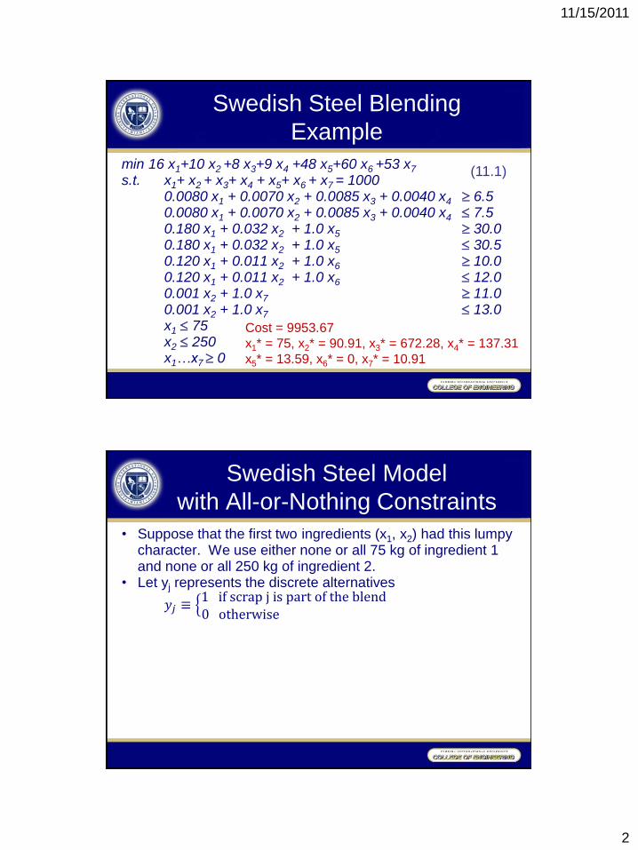
min 16 x1+10 x2 +8 x3+9 x4 +48 x5+60 x6 +53 x7 s.t. x1+ x2 + x3+ x4 + x5+ x6 + x7 = 1000 0.0080 x1 + 0.0070 x2 + 0.0085 x3 + 0.0040 x4 6.5
0.0080 x1 + 0.0070 x2 + 0.0085 x3 + 0.0040 x4 7.5 0.180 x1 + 0.032 x2 + 1.0 x5 30.0 0.180 x1 + 0.032 x2 + 1.0 x5 30.5 0.120 x1 + 0.011 x2 + 1.0 x6 10.0 0.120 x1 + 0.011 x2 + 1.0 x6 12.0 0.001 x2 + 1.0 x7 11.0 0.001 x2 + 1.0 x7 13.0 x1 75 x2 250 x1…x7 0
(11.1)
Cost = 9953.67
x1* = 75, x2* = 90.91, x3* = 672.28, x4* = 137.31
x5* = 13.59, x6* = 0, x7* = 10.91
Swedish Steel Model
with All-or-Nothing Constraints
• Suppose that the first two ingredients (x1, x2) had this lumpy character. We use either none or all 75 kg of ingredient 1 and none or all 250 kg of ingredient 2.
• Let yj represents the discrete alternatives
𝑦𝑗 ≡ 1 if scrap j is part of the blend0 otherwise
11/15/2011
3
Swedish Steel Model
with All-or-Nothing Constraints
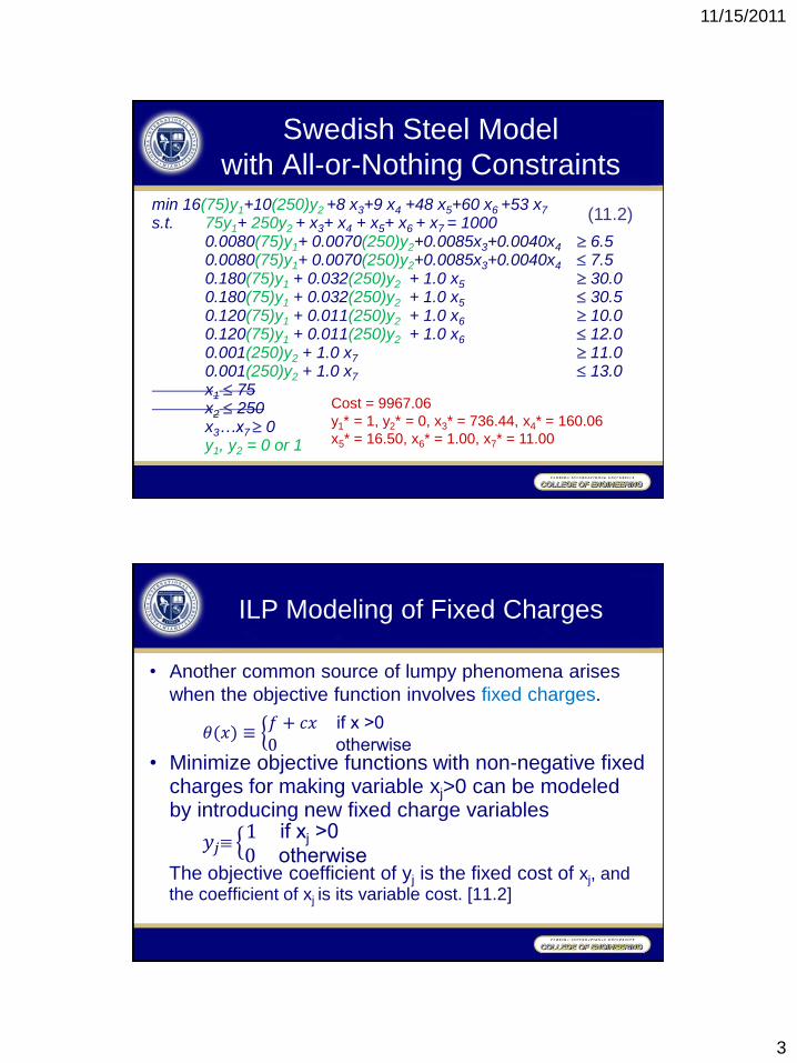
min 16(75)y1+10(250)y2 +8 x3+9 x4 +48 x5+60 x6 +53 x7 s.t. 75y1+ 250y2 + x3+ x4 + x5+ x6 + x7 = 1000 0.0080(75)y1+ 0.0070(250)y2+0.0085x3+0.0040x4 6.5
0.0080(75)y1+ 0.0070(250)y2+0.0085x3+0.0040x4 7.5 0.180(75)y1 + 0.032(250)y2 + 1.0 x5 30.0 0.180(75)y1 + 0.032(250)y2 + 1.0 x5 30.5 0.120(75)y1 + 0.011(250)y2 + 1.0 x6 10.0 0.120(75)y1 + 0.011(250)y2 + 1.0 x6 12.0 0.001(250)y2 + 1.0 x7 11.0 0.001(250)y2 + 1.0 x7 13.0 x1 75 x2 250 x3…x7 0 y1, y2 = 0 or 1
(11.2)
Cost = 9967.06
y1* = 1, y2* = 0, x3* = 736.44, x4* = 160.06
x5* = 16.50, x6* = 1.00, x7* = 11.00
ILP Modeling of Fixed Charges
• Another common source of lumpy phenomena arises
when the objective function involves fixed charges.
𝜃(𝑥) ≡ 𝑓 + 𝑐𝑥 if x >0 0 otherwise
• Minimize objective functions with non-negative fixed charges for making variable xj>0 can be modeled by introducing new fixed charge variables
𝑦𝑗 1 if xj >0 0 otherwise
The objective coefficient of yj is the fixed cost of xj, and the coefficient of xj is its variable cost. [11.2]
11/15/2011
4
ILP Modeling of Fixed Charges
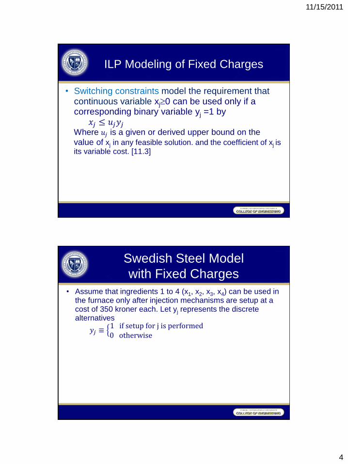
• Switching constraints model the requirement that continuous variable xj0 can be used only if a corresponding binary variable yj =1 by
𝑥𝑗 ≤ 𝑢𝑗𝑦𝑗 Where 𝑢𝑗 is a given or derived upper bound on the
value of xj in any feasible solution. and the coefficient of xj is its variable cost. [11.3]
Swedish Steel Model
with Fixed Charges
• Assume that ingredients 1 to 4 (x1, x2, x3, x4) can be used in the furnace only after injection mechanisms are setup at a cost of 350 kroner each. Let yj represents the discrete alternatives
𝑦𝑗 ≡ 1 if setup for j is performed0 otherwise
11/15/2011
5
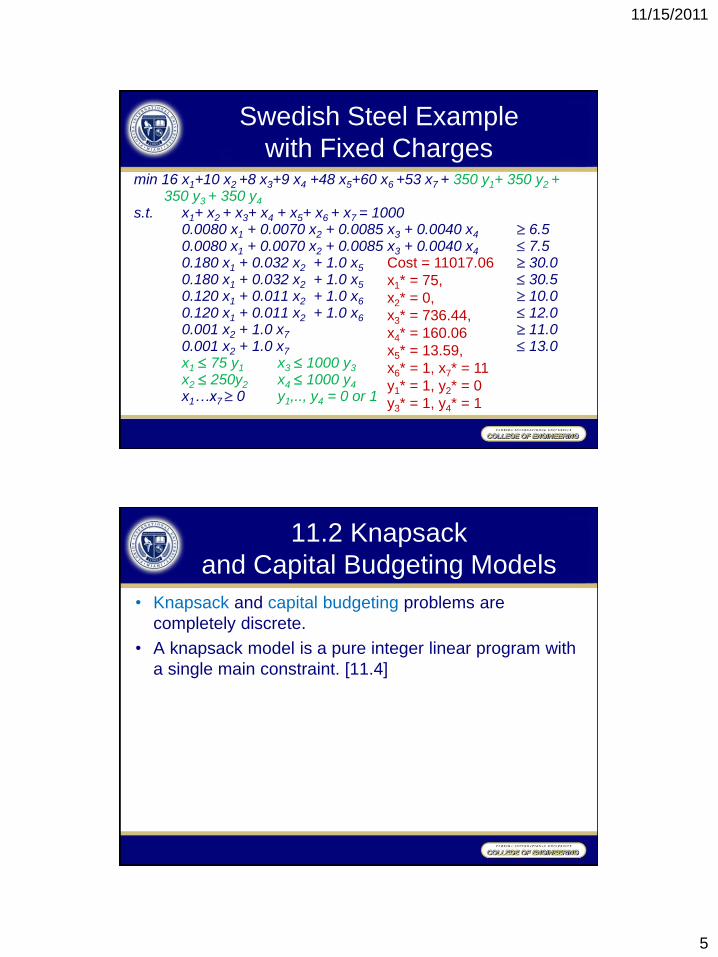
Swedish Steel Example
with Fixed Charges min 16 x1+10 x2 +8 x3+9 x4 +48 x5+60 x6 +53 x7 + 350 y1+ 350 y2 +
350 y3 + 350 y4 s.t. x1+ x2 + x3+ x4 + x5+ x6 + x7 = 1000 0.0080 x1 + 0.0070 x2 + 0.0085 x3 + 0.0040 x4 6.5
0.0080 x1 + 0.0070 x2 + 0.0085 x3 + 0.0040 x4 7.5 0.180 x1 + 0.032 x2 + 1.0 x5 30.0 0.180 x1 + 0.032 x2 + 1.0 x5 30.5 0.120 x1 + 0.011 x2 + 1.0 x6 10.0 0.120 x1 + 0.011 x2 + 1.0 x6 12.0 0.001 x2 + 1.0 x7 11.0 0.001 x2 + 1.0 x7 13.0 x1 75 y1 x3 1000 y3
x2 250y2 x4 1000 y4
x1…x7 0 y1,.., y4 = 0 or 1
Cost = 11017.06
x1* = 75,
x2* = 0,
x3* = 736.44,
x4* = 160.06
x5* = 13.59,
x6* = 1, x7* = 11
y1* = 1, y2* = 0
y3* = 1, y4* = 1
11.2 Knapsack
and Capital Budgeting Models
• Knapsack and capital budgeting problems are
completely discrete.
• A knapsack model is a pure integer linear program with
a single main constraint. [11.4]
11/15/2011
6
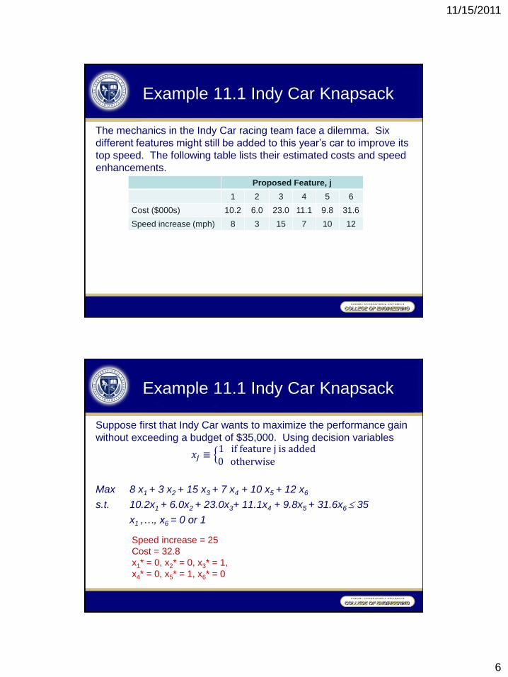
Example 11.1 Indy Car Knapsack
The mechanics in the Indy Car racing team face a dilemma. Six
different features might still be added to this year’s car to improve its
top speed. The following table lists their estimated costs and speed
enhancements.
Proposed Feature, j
1 2 3 4 5 6
Cost ($000s) 10.2 6.0 23.0 11.1 9.8 31.6
Speed increase (mph) 8 3 15 7 10 12
Example 11.1 Indy Car Knapsack
Suppose first that Indy Car wants to maximize the performance gain
without exceeding a budget of $35,000. Using decision variables
𝑥𝑗 ≡ 1 if feature j is added0 otherwise
Max 8 x1 + 3 x2 + 15 x3 + 7 x4 + 10 x5 + 12 x6
s.t. 10.2x1 + 6.0x2 + 23.0x3+ 11.1x4 + 9.8x5 + 31.6x6 35
x1 ,…, x6 = 0 or 1
Speed increase = 25
Cost = 32.8
x1* = 0, x2* = 0, x3* = 1,
x4* = 0, x5* = 1, x6* = 0

11/15/2011
7
Example 11.1 Indy Car Knapsack
Suppose now that the Indy Car team decides they simply must
increase speed by 30 miles per hour to have any chance of winning
the next race. Ignoring the budget, they wish to find the minimum
cost way to achieve at least that much performance.
Min 10.2x1 + 6.0x2 + 23.0x3+ 11.1x4 + 9.8x5 + 31.6x6
s.t. 8 x1 + 3 x2 + 15 x3 + 7 x4 + 10 x5 + 12 x6 30
x1 ,…, x6 = 0 or 1
Cost = 43.0
Speed increase = 33
x1* = 1, x2* = 0, x3* = 1,
x4* = 0, x5* = 1, x6* = 0
Capital Budgeting Models
• The typical maximize form of a knapsack problem has a
single main constraint enforcing a budget.
• Capital budgeting models (or multi-dimensional
knapsack) select a maximum value collection of project,
investments, and so on, subject to limitations on
budgets or other resources consumed. [11.5]
11/15/2011
8
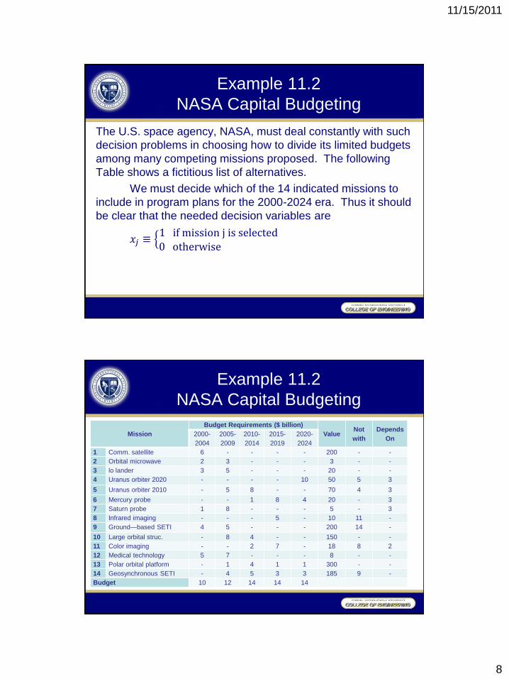
Example 11.2
NASA Capital Budgeting
The U.S. space agency, NASA, must deal constantly with such
decision problems in choosing how to divide its limited budgets
among many competing missions proposed. The following
Table shows a fictitious list of alternatives.
We must decide which of the 14 indicated missions to
include in program plans for the 2000-2024 era. Thus it should
be clear that the needed decision variables are
𝑥𝑗 ≡ 1 if mission j is selected0 otherwise
Example 11.2
NASA Capital Budgeting
Mission
Budget Requirements ($ billion)
Value Not
with
Depends
On 2000-
2004
2005-
2009
2010-
2014
2015-
2019
2020-
2024
1 Comm. satellite 6 - - - - 200 - -
2 Orbital microwave 2 3 - - - 3 - -
3 lo lander 3 5 - - - 20 - -
4 Uranus orbiter 2020 - - - - 10 50 5 3
5 Uranus orbiter 2010 - 5 8 - - 70 4 3
6 Mercury probe - - 1 8 4 20 - 3
7 Saturn probe 1 8 - - - 5 - 3
8 Infrared imaging - - - 5 - 10 11 -
9 Ground—based SETI 4 5 - - - 200 14 -
10 Large orbital struc. - 8 4 - - 150 - -
11 Color imaging - - 2 7 - 18 8 2
12 Medical technology 5 7 - - - 8 - -
13 Polar orbital platform - 1 4 1 1 300 - -
14 Geosynchronous SETI - 4 5 3 3 185 9 -
Budget 10 12 14 14 14

11/15/2011
9
Capital Budgeting Models
• Budget constraints limit the total funds or other resources
consumed by selected projects, investments, and so on, in
each time period not to exceed the amount available. [11.6]
6x1 + 2x2 + 3x3 + 1x7 + 4x9 + 5x12 10
3x2 + 5x3 + 5x5 + 8x7 + 5x9 + 8x10 + 7x12 + 1x13 + 4x14 12
8x5 + 1x6 + 4x10 + 2x11 + 4x13 + 5x14 14
8x6 + 5x8 + 7x11 + 1x13 + 3x14 14
10x4 + 4x6 + 1x13 + 3x14 14
Capital Budgeting Models
• Mutually exclusiveness
conditions allowing at
most one of a set of
choices are modeled by 𝑥𝑗 ≤ 1 constraints
summing over each
choice set. [11.7]
x4 + x5 1
x8 + x11 1
x9 + x14 1
• Dependence of choice j
on choice i can be
enforced on
corresponding binary
variables by constraint
𝑥𝑗 ≤ 𝑥𝑖 [11.8]
x11 x2
x4 x3
x5 x3
x6 x3
x7 x3

11/15/2011
10
NASA Example Model
max 200x1+3x2 +20x3+50x4 +70x5+20 x6 +5x7+10x8+200x9 +150x10+18x11 +8x12 +300x13+185x14
s.t. 6x1 + 2x2 + 3x3 + 1x7 + 4x9 + 5x12 10
3x2 + 5x3 + 5x5 + 8x7 + 5x9 + 8x10 + 7x12 + 1x13 + 4x14 12
8x5 + 1x6 + 4x10 + 2x11 + 4x13 + 5x14 14
8x6 + 5x8 + 7x11 + 1x13 + 3x14 14
10x4 + 4x6 + 1x13 + 3x14 14
x4 + x5 1
x8 + x11 1
x9 + x14 1
xi = 0 or 1 j=1,…,14
(11.7)
x11 x2
x4 x3
x5 x3
x6 x3
x7 x3
x1* = x3* = x4* = x8*
= x13* = x14* =1
Value = 765
11.3 Set Packing, Covering,
and Partitioning Models
• Set covering constraints requiring that at least one
member of sub-collection J belongs to a solution are
expressed [11.9]
𝑥𝑗 ≥ 1
𝑗∈𝐽
• Set packing constraints requiring that at most one
member of sub-collection J belongs to a solution are
expressed [11.10]
𝑥𝑗 ≤ 1
𝑗∈𝐽

11/15/2011
11
11.3 Set Packing, Covering,
and Partitioning Models
• Set partitioning constraints requiring that exactly one
member of sub-collection J belongs to a solution are
expressed [11.11]
𝑥𝑗 = 1
𝑗∈𝐽
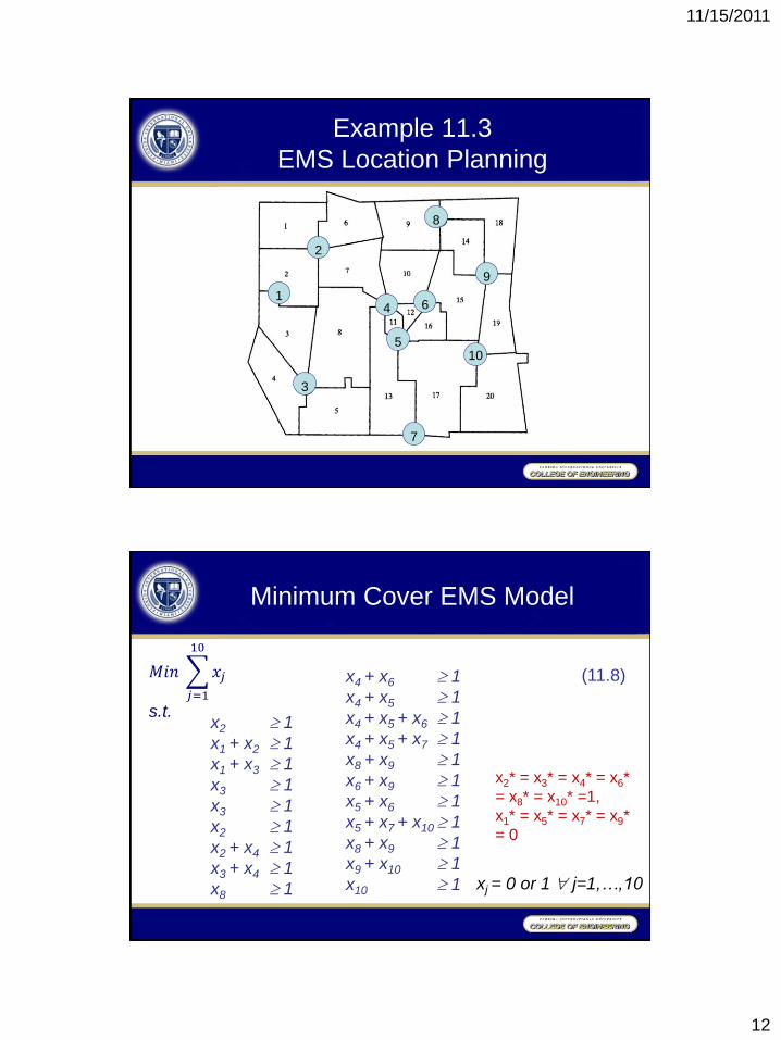
Example 11.3
EMS Location Planning
Austin, Texas undertook a study of the positioning of its
emergency medical service (EMS) vehicles. That city was divided
into service districts needing EMS services, and vehicle stations
selected from a list of alternatives so that as much of the population
as possible would experience a quick response to calls for help.
Our city is divided into 20 service districts that we wish to
serve from some combination of the 10 indicated possibilities for
EMS stations. Each station can provide service to all adjacent
districts. For example, station 2 could service districts 1. 2. 6, and 7.
Main decision variables are
𝑥𝑗 ≡ 1 if location j is selected0 otherwise
11/15/2011
12
Example 11.3
EMS Location Planning
1
2
3
4
5
6
7
8
9
10
Minimum Cover EMS Model
𝑀𝑖𝑛 𝑥𝑗
10
𝑗=1
s.t.
(11.8)
x2 1
x1 + x2 1
x1 + x3 1
x3 1
x3 1
x2 1
x2 + x4 1
x3 + x4 1
x8 1 xj = 0 or 1 j=1,…,10
x4 + x6 1
x4 + x5 1
x4 + x5 + x6 1
x4 + x5 + x7 1
x8 + x9 1
x6 + x9 1
x5 + x6 1
x5 + x7 + x10 1
x8 + x9 1
x9 + x10 1
x10 1
x2* = x3* = x4* = x6*
= x8* = x10* =1,
x1* = x5* = x7* = x9*
= 0
11/15/2011
13
Example 11.3
EMS Location Planning
with Maximum Coverage
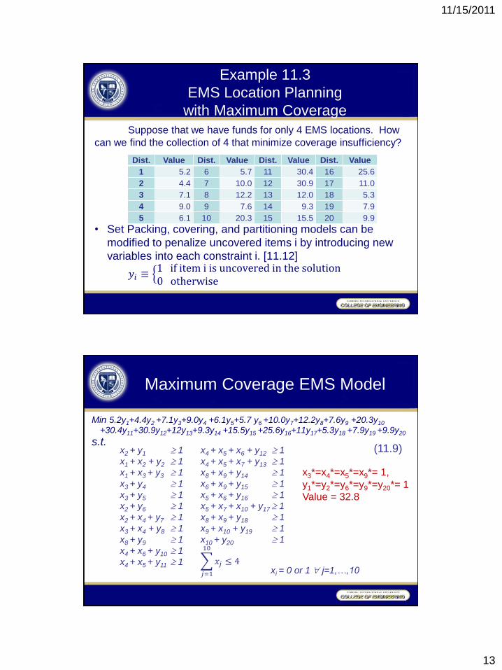
Suppose that we have funds for only 4 EMS locations. How
can we find the collection of 4 that minimize coverage insufficiency?
• Set Packing, covering, and partitioning models can be
modified to penalize uncovered items i by introducing new
variables into each constraint i. [11.12]
𝑦𝑖 ≡ 1 if item i is uncovered in the solution0 otherwise
Dist. Value Dist. Value Dist. Value Dist. Value
1 5.2 6 5.7 11 30.4 16 25.6
2 4.4 7 10.0 12 30.9 17 11.0
3 7.1 8 12.2 13 12.0 18 5.3
4 9.0 9 7.6 14 9.3 19 7.9
5 6.1 10 20.3 15 15.5 20 9.9
Maximum Coverage EMS Model
Min 5.2y1+4.4y2 +7.1y3+9.0y4 +6.1y5+5.7 y6 +10.0y7+12.2y8+7.6y9 +20.3y10
+30.4y11+30.9y12+12y13+9.3y14 +15.5y15 +25.6y16+11y17+5.3y18 +7.9y19 +9.9y20
s.t.
(11.9) x2 + y1 1
x1 + x2 + y2 1
x1 + x3 + y3 1
x3 + y4 1
x3 + y5 1
x2 + y6 1
x2 + x4 + y7 1
x3 + x4 + y8 1
x8 + y9 1
x4 + x6 + y10 1
x4 + x5 + y11 1 xi = 0 or 1 j=1,…,10
x4 + x5 + x6 + y12 1
x4 + x5 + x7 + y13 1
x8 + x9 + y14 1
x6 + x9 + y15 1
x5 + x6 + y16 1
x5 + x7 + x10 + y17 1
x8 + x9 + y18 1
x9 + x10 + y19 1
x10 + y20 1
𝑥𝑗 ≤ 4
10
𝑗=1
x3*=x4*=x5*=x9*= 1,
y1*=y2*=y6*=y9*=y20*= 1
Value = 32.8

11/15/2011
14
Column Generation Models
• Column generation approaches deal with complex
combinatorial problems by first enumerating a
sequence of columns representing viable solutions to
parts of the problem, and then solving a set of
partitioning (or covering or packing) model to select an
optimal collection of these alternatives fulfilling all
problem requirements. [11.13]
Example 11.4
AA Crew Scheduling
A classic application of column generation arises in the
enormously complex problem of scheduling crews for airlines. For
example, American Airlines reports spending over $1.3 billion per
year on salaries, benefits, and travel expenses of air crews. Careful
scheduling or crew pairing can produce enormous savings.
Figure 11.2 illustrates a (tiny) sequence of flights to be
crewed in our fictitious case. Each pairing is a sequence of flights to
be covered by a single crew over a 2- to 3-day period. It must begin
and end in the base city where the crew resides.
In real applications, intricate government and union rules
regulate exactly which sequences of flights constitute a reasonable
pairing. Complex software is employed to generate a list such as
that of Table 11.3. Here we simply allow all closed sequences of 3 or
4 flights in Figure 11.2.
Pairing

11/15/2011
15
Example 11.4
AA Crew Scheduling
MIA
CHI
CHR
DFW
101
402
203
204
305 406
407
308
310
109
211
212
j Flight Sequence Cost
1 101-203-406-308 2900
2 101-203-407 2700
3 101-204-305-407 2600
4 101-204-308 3000
5 203-406-310 2600
6 203-407-109 3150
7 204-305-407-109 2550
8 204-308-109 2500
9 305-407-109-212 2600
10 308-109-212 2050
11 402-204-305 2400
12 402-204-310-211 3600
13 406-308-109-211 2550
14 406-310-211 2650
15 407-109-211 2350
Example 11.4
AA Crew Scheduling
Pairing costs are equally complex. On duty crews are
guaranteed pay for minimum periods, regardless of the part of that
time they are actually flying. If the pairing requires overnight stays
away from home, hotel and other expenses are added. Values for
our illustration are shown in Table 11.3.
The decision variables are defined as
𝑥𝑗 ≡ 1 if pairing j is selected0 otherwise
11/15/2011
16
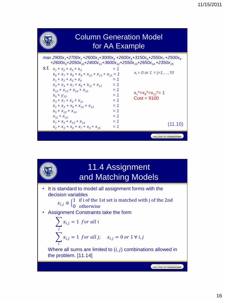
Column Generation Model
for AA Example
max 2900x1+2700x2 +2600x3+3000x4 +2600x5+3150x6+2550x7 +2500x8
+2600x9+2050x10+2400x11+3600x12+2550x13+2650x14 +2350x15
s.t.
(11.10)
x1 + x2 + x3 + x4 = 1
x6 + x7 + x8 + x9 + x10 + x13 + x15 = 1
x1 + x2 + x5 + x6 = 1
x3 + x4 + x7 + x8 + x11 + x12 = 1
x12 + x13 + x14 + x15 = 1
x9 + y10 = 1
x3 + x7 + x9 + x11 = 1
x1 + x4 + x8 + x10 + x13 = 1
x5 + x12 + x14 = 1
x11 + x12 = 1
x1 + x5 + x13 + x14 = 1
x2 + x3 + x6 + x7 + x9 + x15 = 1
xi = 0 or 1 j=1,…,10
x1*=x9*=x12*= 1
Cost = 9100
• It is standard to model all assignment forms with the
decision variables
𝑥𝑖,𝑗 ≡ 1 if i of the 1st set is matched with j of the 2nd0 otherwise
• Assignment Constraints take the form
𝑥𝑖,𝑗 = 1 𝑓𝑜𝑟 𝑎𝑙𝑙 𝑖
𝑗
𝑥𝑖,𝑗 = 1 𝑓𝑜𝑟 𝑎𝑙𝑙 𝑗; 𝑥𝑖,𝑗 = 0 𝑜𝑟 1 ∀ 𝑖, 𝑗
𝑖
Where all sums are limited to (𝑖, 𝑗) combinations allowed in
the problem. [11.14]
11.4 Assignment
and Matching Models

11/15/2011
17
CAM Linear Assignment Example
Revisited
CAM model in Section 10.5 illustrates one assignment case.
The following table repeats total transportation, queuing, and processing
time for 8 pending jobs on 10 workstations to which they might next be
routed. Each workstation can accommodate only one job at a time. We
want to find a minimum total time routing.
Job, i Next Workstation, j
j=1 j=2 j=3 j=4 j=5 j=6 j=7 j=8 j=9 j=10
i=1 8 23 5
i=2 4 12 15
i=3 20 13 6 8
i=4 19 10
i=5 8 12 16
i=6 14 8 3
i=7 6 27 12
i=8 5 15 32
CAM Linear Assignment Model
min 8x1,1+23x1,3 +5x1,9+4x2,2 +12x2,4+15x2,5+20x3,3 +13x3,5 +6x3,6+8x3,8
+19x4,5 +10x4,6 +8x5,4+12x5,7+16x5,10+14x6,1+8x6,7 +3x6,9
+6x7,2+27x7,8+12x7,10 +5x8,2+15x8,3 +32x8,8
s.t.
(11.11)
x1,1 + x1,3 + x1,9 = 1
x2,2 + x2,4 + x2,5 = 1
⋮ x10,1 + x10,2 + x10,3 + x10,4 + x10,5 + x10,6
+ x10,7 + x10,8 + x10,9 + x10,10 = 1
Xi,j = 0 or 1 i=1,…,10; j=1,…,10
x1,1*=x2,2*=x3,8*=x4,6*=
x5,4*=x6,9*=x7,10*=x8,3*= 1
Total Time = 68 x1,1 + x6,1 + x9,1 + x10,1 = 1
x2,2 + x7,2 + x8,2 + x9,2 + x10,2 = 1
⋮ x5,10 + x7,10 + x9,10 + x10,10 = 1
11/15/2011
18
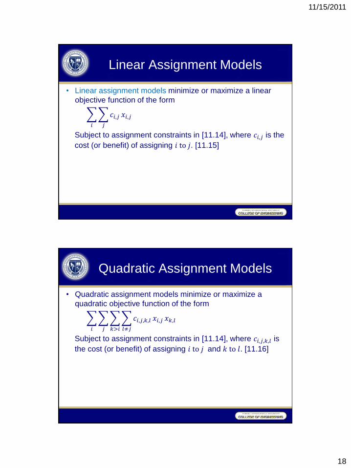
• Linear assignment models minimize or maximize a linear
objective function of the form
𝑐𝑖,𝑗𝑗
𝑥𝑖,𝑗
𝑖
Subject to assignment constraints in [11.14], where 𝑐𝑖,𝑗 is the
cost (or benefit) of assigning 𝑖 to 𝑗. [11.15]
Linear Assignment Models
• Quadratic assignment models minimize or maximize a
quadratic objective function of the form
𝑐𝑖,𝑗,𝑘,𝑙𝑙≠𝑗𝑘>𝑖
𝑥𝑖,𝑗
𝑗
𝑥𝑘,𝑙
𝑖
Subject to assignment constraints in [11.14], where 𝑐𝑖,𝑗,𝑘,𝑙 is
the cost (or benefit) of assigning 𝑖 to 𝑗 and 𝑘 to 𝑙. [11.16]
Quadratic Assignment Models
11/15/2011
19
Example 11.5
Mall Layout Quadratic Assignment
Some of the most common cases producing quadratic
assignment models arise in facility layout. We are given a collection
of machines, offices, departments, stores, and so on, to arrange
within a facility, and a set of locations within which they must fit. The
problem is to decide which unit to assign to each location.
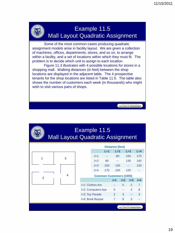
Figure 11.3 illustrates with 4 possible locations for stores in a
shopping mall. Walking distances (in feet) between the shop
locations are displayed in the adjacent table. The 4 prospective
tenants for the shop locations are listed in Table 11.5. The table also
shows the number of customers each week (in thousands) who might
wish to visit various pairs of shops.
Example 11.5
Mall Layout Quadratic Assignment
1
2
3
4
L=1 L=2 L=3 L=4
J=1 -- 80 150 170
J=2 80 -- 130 100
J=3 150 130 -- 120
J=4 170 100 120 --
Distance (feet)
Common Customers (1000)
i=1 i=2 i=3 i=4
i=1: Clothes Are -- 5 2 7
i=2: Computers Aye 5 -- 3 8
i=3: Toy Parade 2 3 -- 3
i=4: Book Bazaar 7 8 3 --
11/15/2011
20
Example 11.5
Mall Layout Quadratic Assignment
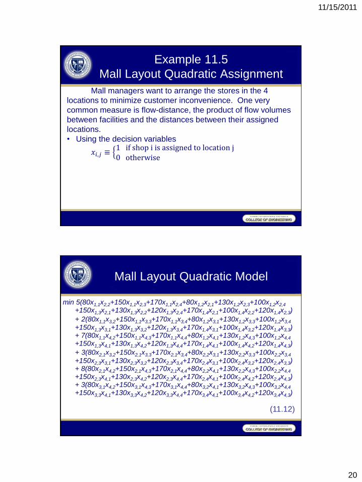
Mall managers want to arrange the stores in the 4
locations to minimize customer inconvenience. One very
common measure is flow-distance, the product of flow volumes
between facilities and the distances between their assigned
locations.
• Using the decision variables
𝑥𝑖,𝑗 ≡ 1 if shop i is assigned to location j0 otherwise
Mall Layout Quadratic Model
min 5(80x1,1x2,2+150x1,1x2,3+170x1,1x2,4+80x1,2x2,1+130x1,2x2,3+100x1,2x2,4
+150x1,3x2,1+130x1,3x2,2+120x1,3x2,4+170x1,4x2,1+100x1,4x2,2+120x1,4x2,3)
+ 2(80x1,1x3,2+150x1,1x3,3+170x1,1x3,4+80x1,2x3,1+130x1,2x3,3+100x1,2x3,4
+150x1,3x3,1+130x1,3x3,2+120x1,3x3,4+170x1,4x3,1+100x1,4x3,2+120x1,4x3,3)
+ 7(80x1,1x4,2+150x1,1x4,3+170x1,1x4,4+80x1,2x4,1+130x1,2x4,3+100x1,2x4,4
+150x1,3x4,1+130x1,3x4,2+120x1,3x4,4+170x1,4x4,1+100x1,4x4,2+120x1,4x4,3)
+ 3(80x2,1x3,2+150x2,1x3,3+170x2,1x3,4+80x2,2x3,1+130x2,2x3,3+100x2,2x3,4
+150x2,3x3,1+130x2,3x3,2+120x2,3x3,4+170x2,4x3,1+100x2,4x3,2+120x2,4x3,3)
+ 8(80x2,1x4,2+150x2,1x4,3+170x2,1x4,4+80x2,2x4,1+130x2,2x4,3+100x2,2x4,4
+150x2,3x4,1+130x2,3x4,2+120x2,3x4,4+170x2,4x4,1+100x2,4x4,2+120x2,4x4,3)
+ 3(80x3,1x4,2+150x3,1x4,3+170x3,1x4,4+80x3,2x4,1+130x3,2x4,3+100x3,2x4,4
+150x3,3x4,1+130x3,3x4,2+120x3,3x4,4+170x3,4x4,1+100x3,4x4,2+120x3,4x4,3)
(11.12)
11/15/2011
21
Mall Layout Quadratic Model
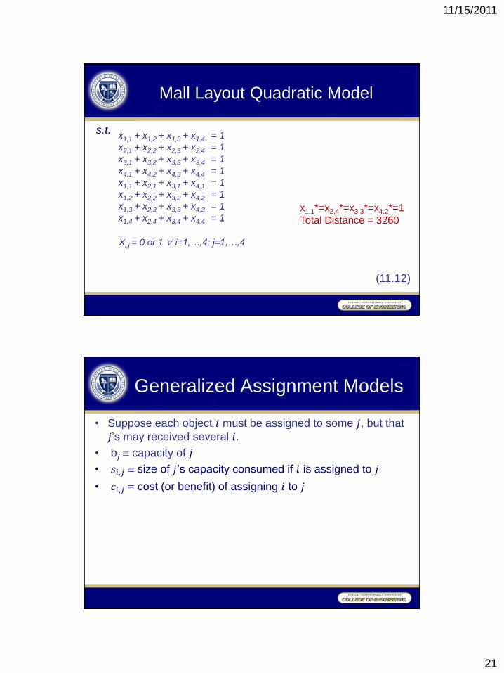
s.t.
(11.12)
x1,1 + x1,2 + x1,3 + x1,4 = 1
x2,1 + x2,2 + x2,3 + x2,4 = 1
x3,1 + x3,2 + x3,3 + x3,4 = 1
x4,1 + x4,2 + x4,3 + x4,4 = 1
x1,1 + x2,1 + x3,1 + x4,1 = 1
x1,2 + x2,2 + x3,2 + x4,2 = 1
x1,3 + x2,3 + x3,3 + x4,3 = 1
x1,4 + x2,4 + x3,4 + x4,4 = 1
Xi,j = 0 or 1 i=1,…,4; j=1,…,4
x1,1*=x2,4*=x3,3*=x4,2*=1
Total Distance = 3260
• Suppose each object 𝑖 must be assigned to some 𝑗, but that
𝑗’s may received several 𝑖.
• b𝑗 capacity of 𝑗
• 𝑠𝑖,𝑗 size of 𝑗’s capacity consumed if 𝑖 is assigned to 𝑗
• 𝑐𝑖,𝑗 cost (or benefit) of assigning 𝑖 to 𝑗
Generalized Assignment Models

11/15/2011
22
• Generalized assignment models, which encompass cases
where allocation of 𝑖 to 𝑗 requires fixed size 𝑠𝑖,𝑗 within
capacity b𝑗 have the form
min𝑜𝑟 𝑚𝑎𝑥 𝑐𝑖,𝑗𝑗
𝑥𝑖,𝑗
𝑖
s.t. 𝑥𝑖,𝑗 = 1 𝑓𝑜𝑟 𝑎𝑙𝑙 𝑖𝑗
𝑥𝑖,𝑗 = 1 𝑓𝑜𝑟 𝑎𝑙𝑙 𝑗; 𝑥𝑖,𝑗 = 0 𝑜𝑟 1 ∀ 𝑖, 𝑗𝑖
Here 𝑐𝑖,𝑗 is the cost (or benefit) of assigning 𝑖 to 𝑗 and all
sums are limited to (𝑖,𝑗) combinations allowed in the
problem. [11.17]
Generalized Assignment Models
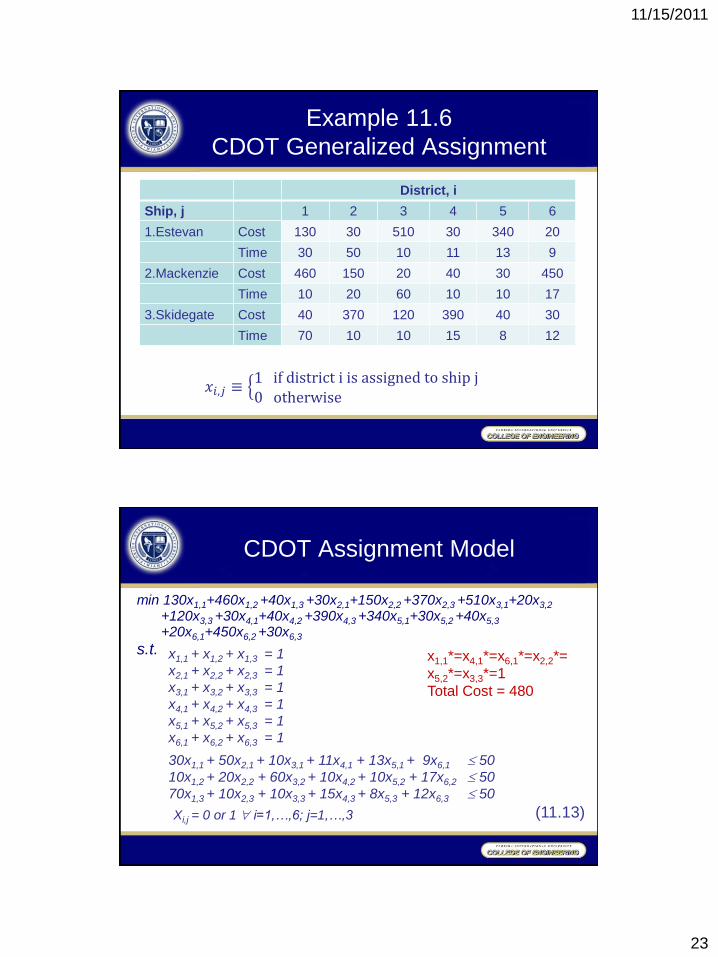
Example 11.6
CDOT Generalized Assignment
The Canadian Department of Transportation encountered a problem
of the generalized assignment form when reviewing their allocation of coast
guard ships on Canada’s Pacific coast. The ships maintain such
navigational aids as lighthouses and buoys. Each of the districts along the
coast is assigned to one of a smaller number of coast guard ships. Since
the ships have different home bases and different equipment and operating
costs, the time and cost for assigning any district varies considerably among
the ships. The task is to find a minimum cost assignment.
Table 11.6 shows data for our (fictitious) version of the problem.
Three ships-the Estevan, the Mackenzie, and the Skidegate--are available to
serve 6 districts. Entries in the table show the number of weeks each ship
would require to maintain aides in each district, together with the annual cost
(in thousands of Canadian dollars). Each ship is available SG weeks per
year.
11/15/2011
23
Example 11.6
CDOT Generalized Assignment
District, i
Ship, j 1 2 3 4 5 6
1.Estevan Cost 130 30 510 30 340 20
Time 30 50 10 11 13 9
2.Mackenzie Cost 460 150 20 40 30 450
Time 10 20 60 10 10 17
3.Skidegate Cost 40 370 120 390 40 30
Time 70 10 10 15 8 12
𝑥𝑖,𝑗 ≡ 1 if district i is assigned to ship j0 otherwise
CDOT Assignment Model
min 130x1,1+460x1,2 +40x1,3 +30x2,1+150x2,2 +370x2,3 +510x3,1+20x3,2
+120x3,3 +30x4,1+40x4,2 +390x4,3 +340x5,1+30x5,2 +40x5,3
+20x6,1+450x6,2 +30x6,3
s.t.
(11.13)
x1,1 + x1,2 + x1,3 = 1
x2,1 + x2,2 + x2,3 = 1
x3,1 + x3,2 + x3,3 = 1
x4,1 + x4,2 + x4,3 = 1
x5,1 + x5,2 + x5,3 = 1
x6,1 + x6,2 + x6,3 = 1
Xi,j = 0 or 1 i=1,…,6; j=1,…,3
x1,1*=x4,1*=x6,1*=x2,2*=
x5,2*=x3,3*=1
Total Cost = 480
30x1,1 + 50x2,1 + 10x3,1 + 11x4,1 + 13x5,1 + 9x6,1 50
10x1,2 + 20x2,2 + 60x3,2 + 10x4,2 + 10x5,2 + 17x6,2 50
70x1,3 + 10x2,3 + 10x3,3 + 15x4,3 + 8x5,3 + 12x6,3 50
11/15/2011
24
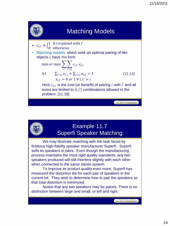
• 𝑥𝑖,𝑖` ≡ 1 if 𝑖 is paired with 𝑖`0 otherwise
• Matching models, which seek an optimal pairing of like
objects 𝑖, have the form
min𝑜𝑟 𝑚𝑎𝑥 𝑐𝑖,𝑖`𝑖`>𝑖
𝑥𝑖,𝑖`
𝑖
s.t. 𝑥𝑖`,𝑖 + 𝑥𝑖,𝑖`𝑖`>𝑖𝑖`<𝑖 = 1
𝑥𝑖,𝑖` = 0 𝑜𝑟 1 ∀ 𝑖, 𝑖` > 𝑖
Here 𝑐𝑖,𝑖` is the cost (or benefit) of pairing 𝑖 with 𝑖` and all
sums are limited to (𝑖,𝑖`) combinations allowed in the
problem. [11.18]
Matching Models
(11.14)
Example 11.7
Superfi Speaker Matching
We may illustrate matching with the task faced by
fictitious high-fidelity speaker manufacturer Superfi. Superfi
sells its speakers in pairs. Even though the manufacturing
process maintains the most rigid quality standards, any two
speakers produced will still interfere slightly with each other
when connected to the same stereo system.
To improve its product quality even more, Superfi has
measured the distortion dw for each pair of speakers in the
current lot. They wish to determine how to pair the speakers so
that total distortion is minimized.
Notice that any two speakers may be paired. There is no
distinction between large and small, or left and right.
11/15/2011
25
Tractability of Assignment and
Matching Models
• Linear assignment models are highly tractable because they
can be viewed as network flow problems, and thus as special
cases of linear programming. Even more efficient special-
purpose algorithms exist. [11.19]
• It is very difficult to compute global optima in quadratic
assignment models because the nonlinear objective function
precludes even the ILP method of Sections 12.2 to 12.5.
Improving search heuristics like those of Sections 12.6 and
12.7 are usually applied. [11.20]
Tractability of Assignment and
Matching Models
• Generalized assignment models, which are ILPs, can be
solved in moderate size by the methods of Sections 12.2 to
12.5. Still, they are far less tractable than the linear
assignment case. [11.21]
• Matching models are more difficult to solve than linear
assignment case but efficient special-purpose algorithms are
known that can solve quite large instances. [11.22]
11/15/2011
26
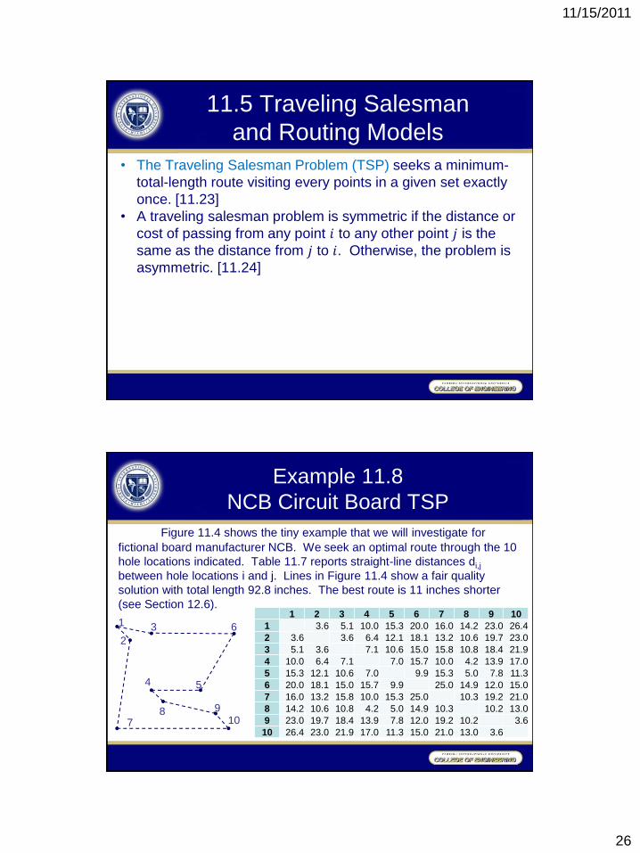
• The Traveling Salesman Problem (TSP) seeks a minimum-
total-length route visiting every points in a given set exactly
once. [11.23]
• A traveling salesman problem is symmetric if the distance or
cost of passing from any point 𝑖 to any other point 𝑗 is the
same as the distance from 𝑗 to 𝑖. Otherwise, the problem is
asymmetric. [11.24]
11.5 Traveling Salesman
and Routing Models
Example 11.8
NCB Circuit Board TSP
Figure 11.4 shows the tiny example that we will investigate for
fictional board manufacturer NCB. We seek an optimal route through the 10
hole locations indicated. Table 11.7 reports straight-line distances di,j
between hole locations i and j. Lines in Figure 11.4 show a fair quality
solution with total length 92.8 inches. The best route is 11 inches shorter
(see Section 12.6). 1 2 3 4 5 6 7 8 9 10
1 3.6 5.1 10.0 15.3 20.0 16.0 14.2 23.0 26.4
2 3.6 3.6 6.4 12.1 18.1 13.2 10.6 19.7 23.0
3 5.1 3.6 7.1 10.6 15.0 15.8 10.8 18.4 21.9
4 10.0 6.4 7.1 7.0 15.7 10.0 4.2 13.9 17.0
5 15.3 12.1 10.6 7.0 9.9 15.3 5.0 7.8 11.3
6 20.0 18.1 15.0 15.7 9.9 25.0 14.9 12.0 15.0
7 16.0 13.2 15.8 10.0 15.3 25.0 10.3 19.2 21.0
8 14.2 10.6 10.8 4.2 5.0 14.9 10.3 10.2 13.0
9 23.0 19.7 18.4 13.9 7.8 12.0 19.2 10.2 3.6
10 26.4 23.0 21.9 17.0 11.3 15.0 21.0 13.0 3.6
1
2
3
4 5
6
7 8 9
10

11/15/2011
27
• Most ILP models of the symmetric case employ decision
variables, 𝑖 < 𝑗
𝑥𝑖,𝑗 ≡ 1 if the route includes a leg between i and j0 otherwise
• Total length of a route can be calculated by
𝑑𝑖,𝑗
𝑗>𝑖
𝑥𝑖,𝑗
𝑖
• Constraints for symmetric TSP
𝑥𝑗,𝑖 +
𝑗<𝑖
𝑥𝑖,𝑗 = 2 𝑓𝑜𝑟 𝑎𝑙𝑙 𝑖
𝑗>𝑖
Formulating the Symmetric TSP
(11.15)
(11.16)
• Definition of subtours
S proper subset of points/cities to
be routed
• Subtour elimination constraints
𝑥𝑖,𝑗 +
𝑖∉𝑆𝑖∈𝑆
𝑥𝑖,𝑗 ≥ 2
𝑖∈𝑆𝑖∉𝑆
• Number of legs between points in S
and points not in S must be at least 2.
Subtours
(11.17)
1
2
3
4 5
6
7
8 9
10
11/15/2011
28
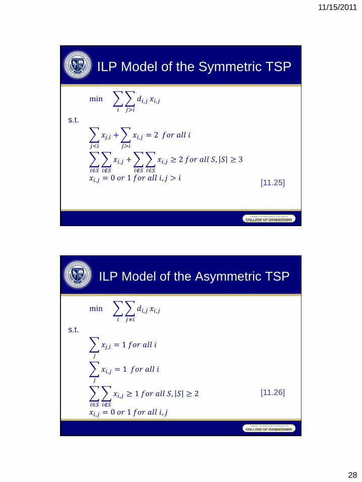
min 𝑑𝑖,𝑗
𝑗>𝑖
𝑥𝑖,𝑗
𝑖
s.t.
𝑥𝑗,𝑖 +
𝑗<𝑖
𝑥𝑖,𝑗 = 2 𝑓𝑜𝑟 𝑎𝑙𝑙 𝑖
𝑗>𝑖
𝑥𝑖,𝑗 +
𝑖∉𝑆𝑖∈𝑆
𝑥𝑖,𝑗 ≥ 2 𝑓𝑜𝑟 𝑎𝑙𝑙 𝑆, 𝑆 ≥ 3
𝑖∈𝑆𝑖∉𝑆
𝑥𝑖,𝑗 = 0 𝑜𝑟 1 𝑓𝑜𝑟 𝑎𝑙𝑙 𝑖, 𝑗 > 𝑖
ILP Model of the Symmetric TSP
[11.25]
min 𝑑𝑖,𝑗
𝑗≠𝑖
𝑥𝑖,𝑗
𝑖
s.t.
𝑥𝑗,𝑖 = 1 𝑓𝑜𝑟 𝑎𝑙𝑙 𝑖
𝑗
𝑥𝑖,𝑗 = 1 𝑓𝑜𝑟 𝑎𝑙𝑙 𝑖
𝑗
𝑥𝑖,𝑗 ≥ 1 𝑓𝑜𝑟 𝑎𝑙𝑙 𝑆, 𝑆 ≥ 2
𝑖∉𝑆𝑖∈𝑆
𝑥𝑖,𝑗 = 0 𝑜𝑟 1 𝑓𝑜𝑟 𝑎𝑙𝑙 𝑖, 𝑗
ILP Model of the Asymmetric TSP
[11.26]
11/15/2011
29
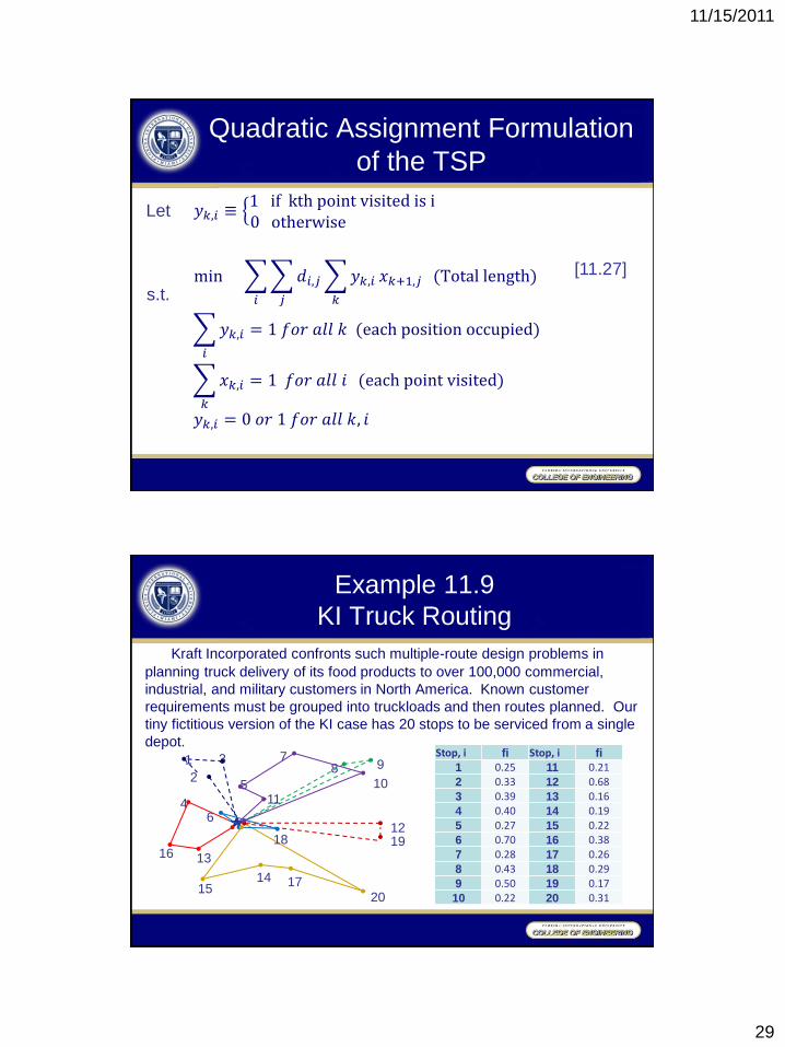
𝑦𝑘,𝑖 ≡ 1 if kth point visited is i0 otherwise
min 𝑑𝑖,𝑗
𝑗
𝑦𝑘,𝑖
𝑘
𝑥𝑘+1,𝑗
𝑖
(Total length)
𝑦𝑘,𝑖 = 1 𝑓𝑜𝑟 𝑎𝑙𝑙 𝑘 (each position occupied)
𝑖
𝑥𝑘,𝑖 = 1 𝑓𝑜𝑟 𝑎𝑙𝑙 𝑖
𝑘
(each point visited)
𝑦𝑘,𝑖 = 0 𝑜𝑟 1 𝑓𝑜𝑟 𝑎𝑙𝑙 𝑘, 𝑖
Quadratic Assignment Formulation
of the TSP
[11.27]
s.t.
Let
Example 11.9
KI Truck Routing
Kraft Incorporated confronts such multiple-route design problems in
planning truck delivery of its food products to over 100,000 commercial,
industrial, and military customers in North America. Known customer
requirements must be grouped into truckloads and then routes planned. Our
tiny fictitious version of the KI case has 20 stops to be serviced from a single
depot.
Stop, i fi Stop, i fi
1 0.25 11 0.21
2 0.33 12 0.68
3 0.39 13 0.16
4 0.40 14 0.19
5 0.27 15 0.22
6 0.70 16 0.38
7 0.28 17 0.26
8 0.43 18 0.29
9 0.50 19 0.17
10 0.22 20 0.31
1
2
3
4
5
6
7 8 9
12 19 18
16 13
11
10
15 14 17
20

11/15/2011
30
Example 11.9
KI Truck Routing
1
2
3
4
5
6
7
8 9
12
19 18
16 13
11
10
15
14 17
20
𝑧𝑖,𝑗 ≡ 1 if stop i is assigned to route j0 otherwise
min 𝜃𝑗
7
𝑗=1
(𝒛)
𝑧𝑖,𝑗 = 1 𝑓𝑜𝑟 𝑎𝑙𝑙 𝑖 = 1,… , 20 (each i to some j)
7
𝑗=1
𝑓𝑖𝑧𝑖,𝑗 ≤ 1 𝑓𝑜𝑟 𝑎𝑙𝑙 𝑖 = 1,… , 7 (truck capacities)
20
𝑖=1
𝑧𝑖,𝑗 = 0 𝑜𝑟 1 𝑓𝑜𝑟 𝑎𝑙𝑙 𝑖, 𝑗
KI Truck Routing Example Model
s.t.
Let
(11.18)
11/15/2011
31
𝜃𝑗(𝒛) ≡ length of the best route through stops assigned to truck j
by decision vector z
• Routing problems are characteristically difficult to represent
concisely in optimization models. [11.28]
KI Truck Routing Example Model
• Fixed charges can be modeled with new binary variables
and switching constraints. Facility Location and Network
Design are common cases of fixed charges.
Facility Location Models
• Facility/plant/warehouse location models choose which of a
proposed list of facilities to open in order to service specified
customer demands at minimum total cost. [11.29]
11.6 Facility Location and
Network Design Models
11/15/2011
32
Example 11.10
Tmark Facilities Location
AT&T has confronted many facility location problems in recommending
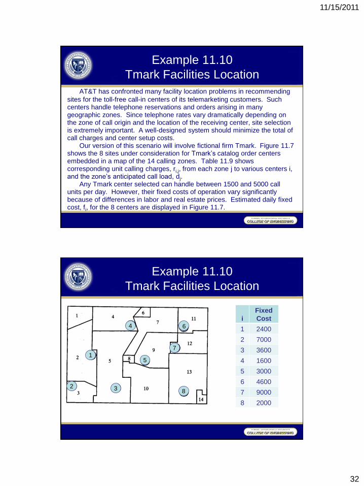
sites for the toll-free call-in centers of its telemarketing customers. Such centers handle telephone reservations and orders arising in many geographic zones. Since telephone rates vary dramatically depending on the zone of call origin and the location of the receiving center, site selection is extremely important. A well-designed system should minimize the total of call charges and center setup costs. Our version of this scenario will involve fictional firm Tmark. Figure 11.7 shows the 8 sites under consideration for Tmark’s catalog order centers embedded in a map of the 14 calling zones. Table 11.9 shows corresponding unit calling charges, ri,j, from each zone j to various centers i, and the zone’s anticipated call load, dj. Any Tmark center selected can handle between 1500 and 5000 call units per day. However, their fixed costs of operation vary significantly because of differences in labor and real estate prices. Estimated daily fixed cost, fi, for the 8 centers are displayed in Figure 11.7.
Example 11.10
Tmark Facilities Location
1
2 3
4
5
6
7
8
i
Fixed
Cost
1 2400
2 7000
3 3600
4 1600
5 3000
6 4600
7 9000
8 2000
11/15/2011
33
Example 11.10
Tmark Facilities Location
Zone
j
Possible Center Location, i Call
Demand 1 2 3 4 5 6 7 8
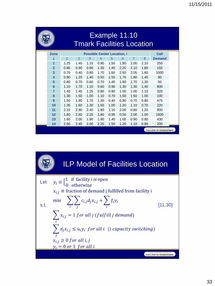
1 1.25 1.40 1.10 0.90 1.50 1.90 2.00 2.10 250
2 0.80 0.90 0.90 1.30 1.40 2.20 2.10 1.80 150
3 0.70 0.40 0.80 1.70 1.60 2.50 2.05 1.60 1000
4 0.90 1.20 1.40 0.50 1.55 1.70 1.80 1.40 80
5 0.80 0.70 0.60 0.70 1.45 1.80 1.70 1.30 50
6 1.10 1.70 1.10 0.60 0.90 1.30 1.30 1.40 800
7 1.40 1.40 1.25 0.80 0.80 1.00 1.00 1.10 325
8 1.30 1.50 1.00 1.10 0.70 1.50 1.50 1.00 100
9 1.50 1.90 1.70 1.30 0.40 0.80 0.70 0.80 475
10 1.35 1.60 1.30 1.50 1.00 1.20 1.10 0.70 220
11 2.10 2.90 2.40 1.90 1.10 2.00 0.80 1.20 900
12 1.80 2.60 2.20 1.80 0.95 0.50 2.00 1.00 1500
13 1.60 2.00 1.90 1.90 1.40 1.00 0.90 0.80 430
14 2.00 2.40 2.00 2.20 1.50 1.20 1.10 0.80 200
𝑦𝑖 ≡ 1 if facility i is open0 otherwise
𝑥𝑖,𝑗 ≡ fraction of demand j fulfilled from facility i
min 𝑐𝑖,𝑗𝑑𝑗𝑥𝑖,𝑗
𝑗
+ 𝑓𝑖𝑦𝑖
𝑖𝑖
𝑥𝑖,𝑗 = 1 𝑓𝑜𝑟 𝑎𝑙𝑙 𝑗 (𝑓𝑢𝑙𝑓𝑖𝑙𝑙 𝑗 𝑑𝑒𝑚𝑎𝑛𝑑)
𝑖
𝑑𝑗𝑥𝑖,𝑗 ≤ 𝑢𝑖𝑦𝑖 𝑓𝑜𝑟 𝑎𝑙𝑙 𝑖
𝑗
(𝑖 𝑐𝑎𝑝𝑎𝑐𝑖𝑡𝑦 𝑠𝑤𝑖𝑡𝑐𝑖𝑛𝑔)
𝑥𝑖,𝑗 ≥ 0 𝑓𝑜𝑟 𝑎𝑙𝑙 𝑖, 𝑗
𝑦𝑖 = 0 𝑜𝑟 1 𝑓𝑜𝑟 𝑎𝑙𝑙 𝑖
ILP Model of Facilities Location
[11.30] s.t.
Let
11/15/2011
34
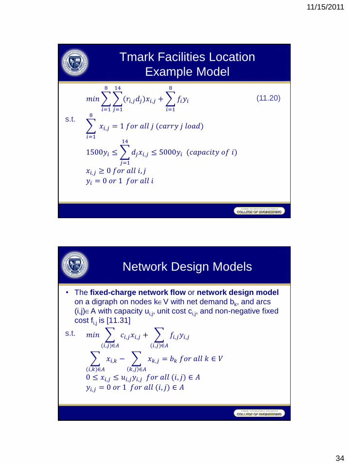
𝑚𝑖𝑛 (𝑟𝑖,𝑗𝑑𝑗)𝑥𝑖,𝑗
14
𝑗=1
+ 𝑓𝑖𝑦𝑖
8
𝑖=1
8
𝑖=1
𝑥𝑖,𝑗
8
𝑖=1
= 1 𝑓𝑜𝑟 𝑎𝑙𝑙 𝑗 (𝑐𝑎𝑟𝑟𝑦 𝑗 𝑙𝑜𝑎𝑑)
1500𝑦𝑖 ≤ 𝑑𝑗𝑥𝑖,𝑗 ≤ 5000𝑦𝑖 (𝑐𝑎𝑝𝑎𝑐𝑖𝑡𝑦 𝑜𝑓 𝑖)
14
𝑗=1
𝑥𝑖,𝑗 ≥ 0 𝑓𝑜𝑟 𝑎𝑙𝑙 𝑖, 𝑗
𝑦𝑖 = 0 𝑜𝑟 1 𝑓𝑜𝑟 𝑎𝑙𝑙 𝑖
Tmark Facilities Location
Example Model
(11.20)
s.t.
• The fixed-charge network flow or network design model
on a digraph on nodes kV with net demand bk, and arcs
(i,j)A with capacity ui,j, unit cost ci,j, and non-negative fixed
cost fi,j is [11.31]
𝑚𝑖𝑛 𝑐𝑖,𝑗𝑥𝑖,𝑗
(𝑖,𝑗)∈𝐴
+ 𝑓𝑖,𝑗𝑦𝑖,𝑗
(𝑖,𝑗)∈𝐴
𝑥𝑖,𝑘 − 𝑥𝑘,𝑗
𝑘,𝑗 ∈𝐴
= 𝑏𝑘 𝑓𝑜𝑟 𝑎𝑙𝑙 𝑘 ∈ 𝑉
(𝑖,𝑘)∈𝐴
0 ≤ 𝑥𝑖,𝑗 ≤ 𝑢𝑖,𝑗𝑦𝑖,𝑗 𝑓𝑜𝑟 𝑎𝑙𝑙 (𝑖, 𝑗) ∈ 𝐴
𝑦𝑖,𝑗 = 0 𝑜𝑟 1 𝑓𝑜𝑟 𝑎𝑙𝑙 (𝑖, 𝑗) ∈ 𝐴
Network Design Models
s.t.

11/15/2011
35
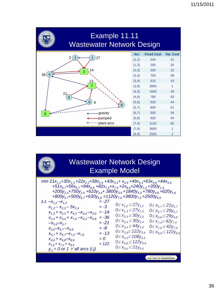
Example 11.11
Wastewater Network Design
Network design applications may involve telecommunications,
electricity, water, gas, coal slurry, or any other substance that flows in a network. We illustrate with an application involving regional wastewater (sewer) networks. As new areas develop around major cities, entire networks of collector sewers and treatment plants must be constructed to service growing population. Figure 11.8 displays our particular (fictional) instance. Nodes 1 to 8 of the network represent population centers where smaller sewers feed into the main regional network, and locations where treatment plants might be built. Wastewater loads are roughly proportional to population, so the inflows indicated at nodes represent population units (in thousands).
Example 11.11
Wastewater Network Design
Arcs joining nodes 1 to 8 show possible routes for main collector
sewers. Most follow the topology in gravity flow, but one pumped line (4. 3) is included. A large part of the construction cost for either type of line is fixed: right-of-way acquisition, trenching, and so on. Still, the cost of a line also grows with the number of population units carried, because greater flows imply larger-diameter pipes. The table in Figure 11.8 shows the fixed and variable cost for each arc in thousand of dollars. Treatment plant costs actually occur at nodes—here nodes 3, 7, and 8. Figure 11.8 illustrates, however, that such costs can be modeled on arcs by introducing an artificial ―supersink" node 9. Costs shown for arcs (3, 9), (7. 9), and (8, 9) capture the fixed and variable expense of plant construction as flows depart the network.
11/15/2011
36
Example 11.11
Wastewater Network Design Arc Fixed Cost Var. Cost
(1,2) 240 21
(1,3) 350 30
(2,3) 200 22
(2,4) 750 58
(3,4) 610 43
(3,9) 3800 1
(4,3) 1840 49
(4,8) 780 63
(5,6) 620 44
(5,7) 800 51
(6,7) 500 56
(6,8) 630 94
(7,4) 1120 82
(7,9) 3800 1
(8,9) 2500 2
1 2
3 4
5
6 9
7
8
27 3
14
36
13
21
8
gravity
pumped
plant arcs
Wastewater Network Design
Example Model
min 21x1,2+30x1,3 +22x2,3+58x2,4 +43x3,4+ x3,9 +49x4,3+63x4,8 +44x5,6 +51x5,7+56x6,7 +94x6,8 +82x7,4+x7,9 +2x8,9+240y1,2 +350y1,3
+200y2,3+750y2,4 +610y3,4+ 3800y3,9 +1840y4,3 +780y4,8 +620y5,6 +800y5,7+500y6,7 +630y6,8 +1120y7,4 +3800y7,9 +2500y8,9
s.t. –x1,2 –x1,3 = -27
x1,2 – x2,3 – 5x2,4 = -3
x1,3 + x2,3 + x4,3 –x3,4 –x3,9 = -14
x2,4 + x3,4 + x7,4 –x4,3 –x4,8 = -36
–x5,6–x5,7 = -21
x5,6–x6,7 –x6,8 = -8
x5,7 + x6,7–x7,4 –x7,9 = -13
x4,8 + x6,8–x8,9 = 0 x3,9 + x7,9 + x8,9 = 122
yi,j = 0 or 1 all arcs (i,j)
0 x1,2 27y1,2
0 x1,3 27y1,3
0 x2,3 30y2,3
0 x2,4 30y2,4
0 x3,4 44y3,4
0 x3,9 122y3,9
0 x4,3 108y4,3
0 x4,8 122y4,8
0 x5,6 21y5,6
0 x5,7 21y5,7
0 x6,7 29y6,7
0 x6,8 29y6,8
0 x7,4 42y7,4
0 x7,9 42y7,9
0 x8,9 122y8,9
11/15/2011
37
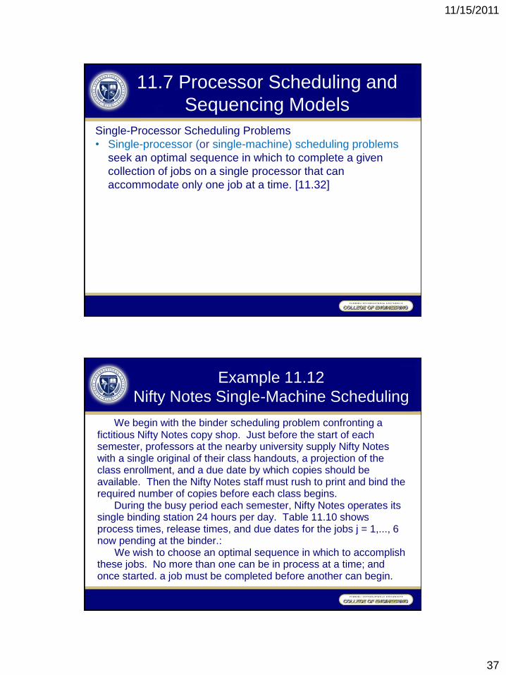
Single-Processor Scheduling Problems
• Single-processor (or single-machine) scheduling problems
seek an optimal sequence in which to complete a given
collection of jobs on a single processor that can
accommodate only one job at a time. [11.32]
11.7 Processor Scheduling and
Sequencing Models
Example 11.12
Nifty Notes Single-Machine Scheduling
We begin with the binder scheduling problem confronting a fictitious Nifty Notes copy shop. Just before the start of each semester, professors at the nearby university supply Nifty Notes with a single original of their class handouts, a projection of the class enrollment, and a due date by which copies should be available. Then the Nifty Notes staff must rush to print and bind the required number of copies before each class begins. During the busy period each semester, Nifty Notes operates its single binding station 24 hours per day. Table 11.10 shows process times, release times, and due dates for the jobs j = 1,..., 6 now pending at the binder.: We wish to choose an optimal sequence in which to accomplish these jobs. No more than one can be in process at a time; and once started. a job must be completed before another can begin.

11/15/2011
38
Example 11.12
Nifty Notes Single-Machine Scheduling
pj estimated process time (in hours) job j will require to bind rj release time (hour) at which job j has/will become available
for processing (relative to time 0 = now) dj = due date (hour) by which job j should be completed (relative
to time 0 = now) Notice that two jobs are already late (dj < 0).
Binder Job, j
1 2 3 4 5 6
Process time, pj 12 8 3 10 4 18
Release time, rj -20 -15 -12 -10 -3 2
Due date, dj 10 2 72 -8 -6 60
• A set of (continuous) decision variables in processor
scheduling models usually determines either the start or the
completion time(s) of each job on the processor(s) it
requires. [11.33]
• xj time binding starts for job j (relative to time 0 = now)
• Constraints on the starting time:
xj max {0, rj}
• Completion time:
(Start time) + (Process time) = (Completion time)
Time Decision Variables
(11.22)
11/15/2011
39
• The central issue in processor scheduling is that only one
job should be in progress on any processor at any time.
• For a pair of jobs j and j’ that might conflict on a processor,
the appropriate conflict constraint is either (11.23)
(start time of j) + (process time of j) (start time of j’), or
(start time of j’) + (process time of j’) (start time of j)
• Conflict avoidance requirement can be modeled explicitly
with the aid of additional disjunctive variables.
• A set of (discrete) disjunctive variables in processor
scheduling models usually determines the sequence in
which jobs are started on processors by specifying whether
each job j is scheduled before or after each other j’ with
which it might conflict. [11.34]
Conflict Constraints and
Disjunctive Variables
• A processor scheduling model with job start time xj and
process time pj can prevent conflicts between jobs j and j’
with disjunctive constraint pairs
xj + pj xj’ + M(1 – yj,j’)
xj’ + pj’ xj + Myj,j’
Where M is a large positive constant, and binary disjunctive
variable yj,j’=1when j is schedule before j’ on the processor
and =0 if j’ is first. [11.35]
Conflict Constraints and
Disjunctive Variables
11/15/2011
40
• Due dates in processor scheduling models are usually
handled as goals to be reflected in the objective function
rather than as explicit constraints. Dates that must be met
are termed deadlines to distinguish. [11.36]
Handling of Due Dates
• Denoting the start time of job j=1,…, n by xj, the process
time by pj, the release time by rj and the due date by dj,
processor scheduling objective functions often minimize one
of the following: [11.37]
• Maximum completion time (makespan) maxj{xj + pj}
Mean completion time (makespan) (1/n)j(xj + pj)
• Maximum flow time maxj{xj + pj - rj}
Mean flow time (1/n)j(xj + pj - rj)
• Maximum lateness maxj{xj + pj - dj}
Mean lateness (1/n)j(xj + pj - dj)
• Maximum tardiness maxj{max[0, xj + pj – dj]}
Mean tardiness (1/n)j(max{0, xj + pj – dj})
Processor Scheduling
Objective Functions
11/15/2011
41
• When any of the minmax objective are being optimized, the
problem is an integer non-linear program (INLP).
• Any of the min max objectives can be linearized by
introducing a new decision variable f to represent the
objective function value, then minimizing f subject to new
constraints of the form f each element in the maximize set.
A similar construction can model tardiness by introducing
new non-negative tardiness variables for each job and
adding constraints keeping each tardiness variable the
corresponding lateness. [11.38]
ILP Formulation of
Minmax Scheduling Objective
• The mean completion time, mean flow time, and mean
lateness scheduling objective functions are equivalent in the
sense that an optimal schedule for one is also optimal for
the others. [11.39]
• An optimal schedule for the maximum lateness objective
function is also optimal for maximum tardiness. [11.40]
Equivalences among
Scheduling Objective Functions

11/15/2011
42
• Job shop scheduling problems seek an optimal schedule for
a given collection of jobs, each of which requires a known
sequence of processors that can accommodate only one job
at a time. [11.41]
Job Shop Scheduling
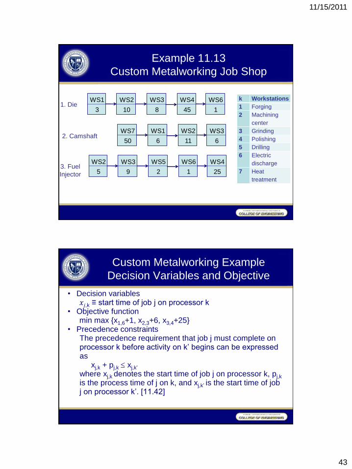
Example 11.13
Custom Metalworking Job Shop
We illustrate job shop scheduling with a fictitious Custom Metalworking company which fabricates prototype metal parts for a nearby engine manufacturer. Figure 11.9 provides details on the 3 jobs waiting to be scheduled. First is a die requiring work on a sequence of 5 workstations: 1 (forging), then 2 (machining), then 3 (grinding), then 4 (polishing), and finally, 6 (electric discharge cutting). Job 2 is a cam shaft requiring 4 stations, and job 3 a fuel injector requiring 5 steps. Numbers in boxes indicate process times Pj,k process time (in minutes) of job j on processor k For example, job 1 requires 45 minutes at polishing workstation 4. Any of the objective function forms in [11.37] could be appropriate for Custom Metalworking’s scheduling. We will assume that the company wants to complete all 3 jobs as soon as possible (minimize maximum completion), so that workers can leave for a holiday.
11/15/2011
43
Example 11.13
Custom Metalworking Job Shop
WS1
3
WS2
10
WS3
8
WS4
45
WS6
1 1. Die
WS7
50
WS1
6
WS2
11
WS3
6 2. Camshaft
WS2
5
WS3
9
WS5
2
WS6
1
WS4
25 3. Fuel
Injector
k Workstations
1 Forging
2 Machining
center
3 Grinding
4 Polishing
5 Drilling
6 Electric
discharge
7 Heat
treatment
Custom Metalworking Example
Decision Variables and Objective
• Decision variables 𝑥𝑗,k ≡ start time of job j on processor k • Objective function min max {x1,6+1, x2,3+6, x3,4+25} • Precedence constraints
The precedence requirement that job j must complete on processor k before activity on k’ begins can be expressed as xj,k + pj,k xj,k’
where xj,k denotes the start time of job j on processor k, pj,k
is the process time of j on k, and xj,k’ is the start time of job j on processor k’. [11.42]

11/15/2011
44
Custom Metalworking Example
Decision Variables and Objective
𝑦𝑗,𝑗′ ,𝑘 ≡ 1 if j is scheduled before job j′ on processor k0 otherwise
• Job shop models can prevent conflicts between jobs by introducing new disjunctive variables yj,j’,k and constraint pair xj,k + pj,k xj,k’ + M (1 - yj,j’,k ) xj’,k + pj’,k xj,k + M yj,j’,k ) For each j, j’ that both require any processor k. Here xj,k
denotes the start time of job j on processor k, pj,k is the process time, M is a large positive constant, and binary yj,j’,k =1 when j is scheduled before j’ on k, and =0 if j’ is first. [11.43]
Custom Metalworking Example Model
min max {x1,6+1, x2,3+6, x3,4+25} s.t. x1,1 +3 x1,2
x1,2 +10 x1,3
x1,3 +8 x1,4
x1,4 +45 x1,6
x2,7 +50 x2,1
x2,1 +6 x2,2
x2,2 +11 x2,3
x3,2 +5 x3,3
x3,3 +9 x3,5
x3,5 +2 x3,6
x3,6 +1 x3,4
x1,1 +3 x2,1+M(1-y1,2,1) x2,1 +6 x1,1+My1,2,1
x1,2 +10 x2,2 +M(1-y1,2,2)
x2,2 +11 x1,2 +My1,2,2
x1,2 +10 x3,2 +M(1-y1,3,2)
x3,2 +5 x1,2 +My1,3,2
x2,2 +11 x3,2 +M(1-y2,3,2)
x3,2 +5 x1,2 +My2,3,2)
x1,3 +8 x2,3 +M(1-y1,2,3)
x2,3 +6 x1,3 +My1,2,3)
x1,3 +8 x3,3 +M(1-y1,3,3)
x3,3 +9 x1,3 +My1,3,3)
x2,3 +6 x3,3+M(1-y2,3,3) x3,3 +9 x2,3+My2,3,3
x1,4 +45 x3,4 +M(1-y1,3,4)
x3,4 +25 x1,4 +My1,3,4
x1,6 +1 x3,6 +M(1-y1,3,6)
x3,6 +1 x1,6 +My1,3,6
xj,k 0
yj,j’,k = 0 or 1