CONTRIBUTED RESEARCH ARTICLE 84

Discrete Time Markov Chains with Rby Giorgio Alfredo Spedicato

Abstract The markovchain package aims to provide S4 classes and methods to easily handle DiscreteTime Markov Chains (DTMCs), filling the gap with what is currently available in the CRAN repository.In this work, I provide an exhaustive description of the main functions included in the package, aswell as hands-on examples.

Introduction

DTMCs are a notable class of stochastic processes. Although their basic theory is not overly complex,they are extremely effective to model categorical data sequences (Ching et al., 2008). To illustrate, no-table applications can be found in linguistic (see Markov’s original paper Markov (1907)), informationtheory (Google original algorithm is based on Markov Chains theory, Lawrence Page et al. (1999)),medicine (transition across HIV severity states, Craig and Sendi (2002)), economics and sociology(Jones (1997) shows an application of Markov Chains to model social mobility).

The markovchain package (Spedicato, Giorgio Alfredo, 2016) provides an efficient tool to create,manage and analyse Markov Chains (MCs). Some of the main features include the possibility to:validate the input transition matrix, plot the transition matrix as a graph diagram, perform structuralanalysis of DTMCs (e.g. classification of transition matrices and states, analysis of the stationarydistribution, etc . . . ), perform statistical inference (such as fitting transition matrices from variousinput data, simulating stochastic processes trajectories from a given DTMC, etc..). The author believesthat no R package provides a unified infrastructure to easily manage DTMCs as markovchain does atthe time this paper is being drafted.

The package targets data scientists using DTMC, Academia members, supporting faculty instruc-tors, as well as students of undergraduate courses on Stochastic Processes.

The paper will be organized as follows: Section 2.2 gives a brief overview on R packages andalternative software that provide similar functionalities, Section 2.3 reviews DTMC basic theory,Section 2.4 discusses the package design and structure, Section 2.5 shows how to create and manipulatehomogeneous DTMCs, Section 2.6 and Section 2.7 respectively present the functions created to performstructural analysis, and statistical inference on DTMCs. A brief overview of the functionalities writtento deal with non - homogeneous discrete dime Markov chains (NHDTMCs) is provided in Section2.8. A discussion on numerical reliability and computational performance is provided in Section 2.9.Finally, Section 2.10 draws final conclusions and briefly discusses future potential developments of thepackage.

Analysis of existing DTMC-related software

As reviewed later in more details, a DTMC is defined by a stochastic matrix known as transition matrix(TM), which is a square matrix satisfying Equation 1.{

Pij ∈ [0, 1] ∀i, j∑i Pij = 1 (1)

Although defining a stochastic matrix is trivial in any mathematical or statistical software, a DTMCdedicated infrastructure can provide object oriented programmed methods to verify the validity of theinput data (i.e. if the input matrix is a stochastic one) , as well as to perform structural analysis onDTMC objects.

Various packages mention MCs - related models in the CRAN repository, whereby a few of themwill be now reviewed. The clickstream package (Scholz, 2016), on CRAN since 2014, aims to modelwebsites click stream using higher order Markov Chains. It provides a MarkovChain S4 class that issimilar to the markovchain class. Further, DTMCPack (Nicholson, William, 2013) and MTCM (Bessi,Alessandro, 2015) also work with DTMCs but provide even more limited functions: the first onefocuses on creating simulations from a given DTMC, whilst the second contains only one function forestimating the underlying transition matrix for a given categorical sequence. Moreover, none of themappears to have been updated since 2015. The coverage of functionalities provided by markovchainpackage for analysing DTMCs appears to be more complete than the above mentioned packages, sincenone of them provides methods for importing or coercing transition matrices from other objects, suchas R matrices or data.frames. Furthermore, markovchain is the only package providing a quickgraph plotting facility for DTMC objects. The same applies when considering the functionalities used

The R Journal Vol. 9/2, December 2017 ISSN 2073-4859

CONTRIBUTED RESEARCH ARTICLE 85

to perform structural analysis of transition matrices and to fit DTMCs from various kind of input data.More interestingly, the FuzzyStatProb package (Pablo J. Villacorta and José L. Verdegay, 2016) givesan alternative approach for estimating the parameters of DTMCs using "fuzzy logic".

This review voluntarily omits discussing packages that are not specifically focused on DTMC.Nonetheless, the depmixS4 (Visser and Speekenbrink, 2010) and the HMM (Himmelmann, 2010)packages deal with Hidden Markov Models (HMMs). In addition, the number of R packages focusedon the estimation of statistical models using the Markov Chain Monte Carlo simulation approachis sensibly bigger. Finally, the msm (Jackson, 2011), heemod (Antoine Filipovi et al., 2017) and theTPmsm packages (Artur Araújo et al., 2014) focus on health applications of multi - state analysis usingdifferent kinds of models, including Markov-related ones among them.

Finally, among other well known software used in Mathematics and Statistics, only Mathematica(Wolfram Research, Inc., 2013) provides routines specifically written to deal with Markov processesat the author’s knowledge. Nevertheless, the analysis of DTMCs could be easily handled within theMatlab programming language (MATLAB, 2017) due to its well known linear algebra capabilities.

Review of underlying theory

In this section a brief review of the theory of DTMCs is presented. Readers willing to dive deeper caninspect Cassandras (1993) and Grinstead and Snell (2012).

A DTMC is a stochastic process whose domain is a discrete set of states, {s1, s2, . . . , sk}. Thechain starts in a generic state at time zero and moves from a state to another by steps. Let pij be theprobability that a chain currently in state si moves to state sj at the next step. The key characteristicof DTMC processes is that pij does not depend upon the previous state in the chain. The probabilitypij for a (finite) DTMC is defined by a transition matrix previously introduced (see Equation 1). It isalso possible to define the TM by column, under the constraint that the sum of the elements in eachcolumn is 1.

To illustrate, a few toy - examples on transition matrices are now presented; the "Land of Oz"weather Matrix, Kemeny et al. (1974). Equation 2 shows the transition probability between (R)ainy,(N)ice and (S)now weathers.

R N SR 0.5 0.25 0.25N 0.5 0 0.5S 0.25 0.25 0.5

(2)

Further, the Mathematica Matrix 3, taken from the Mathematica 9 Computer Algebra Systemmanual (Wolfram Research, Inc., 2013), that will be used when discussing the analysis the structuralproprieties of DTMCs, is as follows:

A B C DA 0.5 0.5 0 0B 0.5 0.5 0 0C 0.25 0.25 0.25 0.25D 0 0 0 1

(3)

Simple operations on TMs allow to understand structural proprieties of DTMCs. For example, then− th power of P is a matrix whose entries represent the probabilities that a DTMC in state si at time twill be in state sj at time t + n. In particular, if ut is the probability vector for time t (that is, a vectorwhose j− th entries represent the probability that the chain will be in the j− th state at time t), thenthe distribution of the chain at time t + n is given by un = u ∗ Pn. Main properties of Markov chainsare now presented.

A state si is reachable from state sj if ∃n→ pnij > 0. If the inverse is also true then si and sj are said

to communicate . For each MC, there always exists a unique decomposition of the state space into asequence of disjoint subsets in which all the states within each subset communicate. Each subset isknown as a communicating class of the MC. It is possible to link this decomposition to graph theory,since the communicating classes represent the strongly connected components of the graph underlyingthe transition matrix (Jarvis and Shier, 1999).

A state sj of a DTMC is said to be absorbing if it is impossible to leave it, meaning pjj = 1. Anabsorbing Markov chain is a chain that contains at least one absorbing state which can be reached, notnecessarily in a single step. Non - absorbing states of an absorbing MC are defined as transient states .In addition, states that can be visited more than once by the MC are known as recurrent states .

If a DTMC contains r ≥ 1 absorbing states, it is possible to re-arrange their order by separating

The R Journal Vol. 9/2, December 2017 ISSN 2073-4859

CONTRIBUTED RESEARCH ARTICLE 86

transient and absorbing states such that the t transient states come before the r absorbing ones. Suchre-arranged matrix is said to be in canonical form (see Equation 4), where its composition can berepresented by sub - matrices. (

Qt,t Rt,r0r,t Ir,r

)(4)

Such matrices are: Q (a t-square sub - matrix containing the transition probabilities across transientstates), R (a nonzero t-by-r matrix containing transition probabilities from non-absorbing to absorbingstates), 0 ( an r-by-t zero matrix), and Ir (an r-by-r identity matrix). It is possible to use these matricesto calculate various structural proprieties of the DTMC. Since limn→∞ Qn = 0, it can be shown that inevery absorbing matrix the probability to be eventually absorbed is 1, regardless of the state where theMC is initiated.

Further, in Equation 5 the fundamental matrix is presented, where the generic nij entry expressesthe expected number of times the process will transit in state sj, given that it started in state si. Also,the i-th entry of vector t = N ∗ 1, being 1 a t-sized vector of ones, expresses the expected number ofsteps before an absorbing DTMC, started in state si, is absorbed. The bij entries of matrix B = N ∗ Rare the probabilities that a DTMC started in state si will eventually be absorbed in state sj. Finally, theprobability of visiting the transient state j when starting from the transient state i is the hij entry of thematrix H = (N − It) ∗ N−1

dg , being dg the diagonal operator.

N = (I −Q)− 1 = I + ∑i=0,1,...,∞

Qi (5)

A DTMC is said to be ergodic if there exist a number N such that it is possible to reach every statein at most N steps. If Pn > 0 for some n, then P is a regular DTMC.

Fixed row vectors w, also known as steady state vectors , are vectors such that wP = w. Mathemat-ically, they correspond to eigenvectors associated to unitary eigenvalues of the TM. It can be shownthat limn→∞ v ∗ Pn = w and that limn→∞ Pn = W, where v is a generic stochastic vector and w is amatrix where all rows are w.

The mean first passage time mij is the expected the number of steps needed to reach state sj startingfrom state si, where mii = 0 by convention. For ergodic MCs, ri is the mean recurrence time, that is theexpected number of steps to return to si from si. It is possible to prove that ri =

1wi

, where wi is the i-thentry of w. Further, let D be a diagonal matrix, in which the diagonal elements come from ri, and let Cbe a matrix filled with ones. It is then possible to get the mean first passage matrix M from Equation 6.

(I − P) = C−M (6)

Let Z = (I − P + M)−1 be the fundamental matrix for an ergodic MC. It is possible to write mij asa function of Z and w, as Equation 7 shows.

mij =zjj − zij

wj(7)

A further topic in structural analysis of irreducible DTMCs is periodicity. The period of a state si,denoted as d (i), is the greatest common divisor of n for which pn

ii > 0. If the period is 1, the state isaperiodic, while if the period is greater than 2, the state is periodic; all states in the same class sharethe same period.

Given a generic DTMC, it is possible to simulate stochastic trajectories following the underlyingMC from the TM. Given an initial state s(t) = j, the s(t + 1) state is sampled from the multinomialdistribution whose probabilities are expressed by the j-th row. The sampled state indicates from whichrow the probabilities to sample s(t + 2) are taken from. Also, given a sample sequence, it is possible toestimate the TM of the underlying DTMC. Equation 8 shows the maximum likelihood estimator (MLE)

of the TM pij entry, being the nij elements the number of sequences(

Xt = si, Xt+1 = sj

)counted in

the sample, that is:

pMLEij =

nijk∑

u=1niu

. (8)

Equation 10 shows asymptotic confidence intervals for pij. The bootstrap approach allows todefine non - parametric ones.

The R Journal Vol. 9/2, December 2017 ISSN 2073-4859

CONTRIBUTED RESEARCH ARTICLE 87

LowerEndpointij = pij − 1.96 ∗ SEij (9)

UpperEndpointij = pij + 1.96 ∗ SEij (10)

The mode of the Xt+1 conditional distribution given Xt = sj represents the prediction from a givenDTMC and the current chain state Xt = sj.

In conclusion, the markovchain package allows to perform statistical analysis on NHDTMCs, inthe special case where they can be treated as sequential lists of DTMCs.

Implementation design and details

The markovchain package has been originally written in "native" R. Most functions have been thereforeported in Rcpp (Eddelbuettel, Dirk, 2013) since 2015, yielding sensible improvements in computationaltime. Other dependencies of markovchain are: igraph Csardi, Gabor and Nepusz, Tamas (2006),matlab Roebuck (2014), Matrix Bates and Maechler (2016) and expm Goulet et al. (2015) ( for operationon matrices ), and the method package for defining S4 classes.

Homogeneous DTMCs are defined by a dedicated S4 class, "markovchain". Such class is definedby the following slots:

1. states: a character vector, listing the states for which transition probabilities are defined.

2. byrow: a logical variable, indicating whether transition probabilities are shown by row or bycolumn.

3. transitionMatrix: a matrix variable defining the TM.

4. name: an optional character variable to name the DTMC.

A "markovchain" S4 class has been designed based on Chambers, J.M. (2008) suggestions. Forexample, a S4 setValidity method checks the coherence of any newly created markovchain object, byverifying that either the rows or columns of the transition matrix sum to one, and that all elements arebounded between 0 and 1.Another S4 class,"markovchainList", has been created for handling non - homogeneous DTMCs.Finally, the package provides functions and S4 to analyse continuous MCs, as well as higher orderMCs, although their discussion is beyond the scope of this paper.

Three vignettes documents the markovchain package. The first one broadly describes the func-tionalities of the package and it also presents real - world applications of DTMCs using the package.The second one, written using knit and rmarkdown, is a beamer presentation that quickly introducesthe key functionalities of the package. The third one presents experimental functions for higher orderand multivariate MCs. Finally, the www.github.com/spedygiorgio/markovchain GitHub page hoststhe package’s wiki as well as its development version.

Creating and manipulating markovchain objects

The package is loaded within R as follows:

library("markovchain")

Creating a markovchain object is easy, and can be done with provided code.

#using "long" approach for mcWeather

weatherStates <- c("rainy", "nice", "sunny")weatherMatrix <- matrix(data = c(0.50, 0.25, 0.25,0.5, 0.0, 0.5, 0.25, 0.25, 0.5), byrow = TRUE,nrow = 3,dimnames = list(weatherStates, weatherStates))mcWeather <- new("markovchain", states = weatherStates,byrow = TRUE, transitionMatrix = weatherMatrix,name = "Weather")

#using "quick" approach on Mathematica's DTMC

mathematicaMatr <- matrix(c(1/2, 1/2, 0, 0, 1/2, 1/2,

The R Journal Vol. 9/2, December 2017 ISSN 2073-4859

CONTRIBUTED RESEARCH ARTICLE 88

0, 0, 1/4, 1/4, 1/4, 1/4, 0, 0, 0, 1),byrow=TRUE, nrow=4)mathematicaMc<-as(mathematicaMatr, "markovchain")

#both are markovchain objectsis(mcWeather,"markovchain")[1] TRUEis(mathematicaMc,"markovchain")[1] TRUE

Commenting on the code snippet, the first part shows the “standard” approach to create amarkovchain, by calling the new S4 method, while the second part shows the “quick” method, bycoercing a matrix object into a markovchain one.

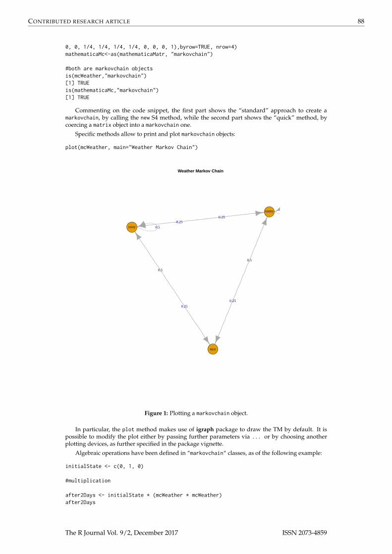
Specific methods allow to print and plot markovchain objects:

plot(mcWeather, main="Weather Markov Chain")

Weather Markov Chain

0.5

0.25

0.25

0.5

0.5

0.25

0.25

rainy

nice

sunny

Figure 1: Plotting a markovchain object.

In particular, the plot method makes use of igraph package to draw the TM by default. It ispossible to modify the plot either by passing further parameters via ... or by choosing anotherplotting devices, as further specified in the package vignette.

Algebraic operations have been defined in "markovchain" classes, as of the following example:

initialState <- c(0, 1, 0)

#multiplication

after2Days <- initialState * (mcWeather * mcWeather)after2Days

The R Journal Vol. 9/2, December 2017 ISSN 2073-4859

CONTRIBUTED RESEARCH ARTICLE 89

rainy nice sunny[1,] 0.375 0.25 0.375

in which multiplications by vectors and exponentiation are intuitively performed, making easy tofind the distribution of states at the n-th step.

A power operator also exists, ^, and it is based on the expm package (Goulet et al., 2015), providingefficient matrix exponentiation.

#after two days (by square power)

mcWeather^2

Weather^2A 3 - dimensional discrete MC defined by the following states:rainy, nice, sunnyThe transition matrix (by rows) is defined as follows:

rainy nice sunnyrainy 0.4375 0.1875 0.3750nice 0.3750 0.2500 0.3750sunny 0.3750 0.1875 0.437

Finally, logical operators have been defined as well.

#logical equality and inequalitymcWeather==mcWeather[1] TRUEmcWeather!=mathematicaMc[1] TRUE

Both the algebraic and logical operators have been defined by overriding standard R operators,providing a more concise and "natural" code, which can bring the advantage of being more appealingto a novice user, by executing certain operations on TM in an efficient way. Such approach has beenstressed in both the class help file and the package vignette code to make the final user fully aware ofany potential drawbacks of such choice.

Various convenience S4 methods have been defined to easily manipulate and manage markovchainobjects. In the following examples, some of the implemented methods in the "markovchain" class arepresented, allowing to: get and set names, return the MC dimension, transpose the transition matrix,and directly access the transition probabilities.

#some markovchain specific methods

#namingname(mcWeather)[1] "Weather"

name(mathematicaMc) <- "Mathematica Markov Chain"#list of defined statesstates(mcWeather)[1] "rainy" "nice" "sunny"

#the dimensiondim(mcWeather)[1] 3

#transpose operatort(mcWeather)

Unnamed Markov chainA 3 - dimensional discrete Markov Chain defined by the following states:rainy, nice, sunnyThe transition matrix (by cols) is defined as follows:

rainy nice sunnyrainy 0.50 0.5 0.25nice 0.25 0.0 0.25

The R Journal Vol. 9/2, December 2017 ISSN 2073-4859

CONTRIBUTED RESEARCH ARTICLE 90

sunny 0.25 0.5 0.50

#two ways to get transition probabilitiestransitionProbability(mcWeather, "nice", "sunny")[1] 0.5mcWeather[2,3][1] 0.5

Finally, coerce methods allow to both import and export markovchain classes. Following, a briefexample on how to transform a markovchain object into a data.frame one.

#exporting to data.frame and matrix

as(mcWeather, "data.frame")t0 t1 prob

1 rainy rainy 0.502 rainy nice 0.253 rainy sunny 0.254 nice rainy 0.505 nice nice 0.006 nice sunny 0.507 sunny rainy 0.258 sunny nice 0.259 sunny sunny 0.50

Structural properties of finite Markov chains

The markovchain package embeds functions to analyse the structural proprieties of DTMC. For exam-ple, it is possible to find the stationary distribution, as well as classify the states. Feres, Renaldo (2007)and Montgomery, James (2009) provide a full description of the algorithms underlying these functions,whilst a more theoretical perspective can be found in Brémaud, Pierre (1999). The Mathematica MCwill be used to illustrate such features.

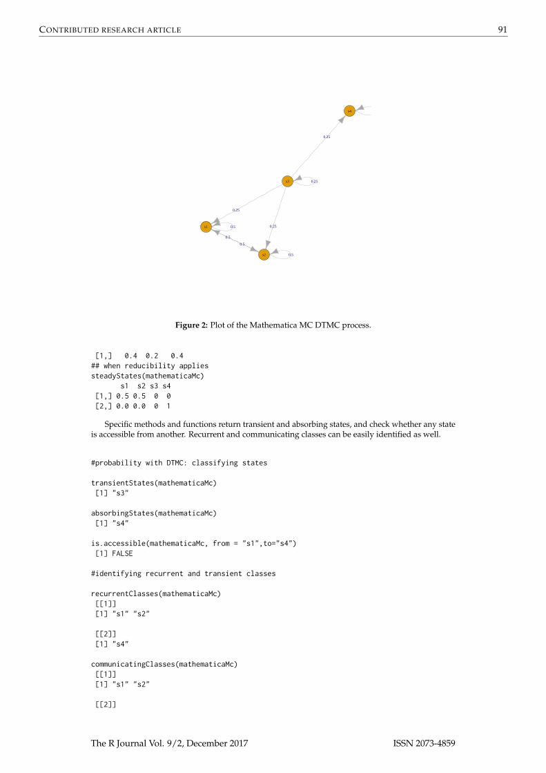
The summary method provides an overview of the structural properties of the DTMC processunderlying the markovchain object.

#plotting and summarizingplot(mathematicaMc)

summary(mathematicaMc)Mathematica Markov Chain Markov chain that is composed by:Closed classes:s1 s2s4Recurrent classes:{s1,s2},{s4}Transient classes:{s3}The Markov chain is not irreducibleThe absorbing states are: s4

In the above example, closed and transient classes are identified, irreducibility checks are executed,and a list of absorbing states is returned. Further, it is known that a finite MC has at least onesteady-state distribution, and the steadyStates method can be used to obtain it. To illustrate, for themcWeather matrix there exist a one - dimensional solution, since the underlying TM is irreducible. Ahigher dimensional solution is given when the irreducibility property does not hold, as of the secondexample.

#probability with DTMC: stationary distribution## when the TM is irreducibilesteadyStates(mcWeather)

rainy nice sunny

The R Journal Vol. 9/2, December 2017 ISSN 2073-4859

CONTRIBUTED RESEARCH ARTICLE 91

0.5

0.5

0.25

0.5

0.5

0.25

0.25

0.25

s1

s2

s3

s4

Figure 2: Plot of the Mathematica MC DTMC process.

[1,] 0.4 0.2 0.4## when reducibility appliessteadyStates(mathematicaMc)

s1 s2 s3 s4[1,] 0.5 0.5 0 0[2,] 0.0 0.0 0 1

Specific methods and functions return transient and absorbing states, and check whether any stateis accessible from another. Recurrent and communicating classes can be easily identified as well.

#probability with DTMC: classifying states

transientStates(mathematicaMc)[1] "s3"

absorbingStates(mathematicaMc)[1] "s4"

is.accessible(mathematicaMc, from = "s1",to="s4")[1] FALSE

#identifying recurrent and transient classes

recurrentClasses(mathematicaMc)[[1]][1] "s1" "s2"

[[2]][1] "s4"

communicatingClasses(mathematicaMc)[[1]][1] "s1" "s2"

[[2]]

The R Journal Vol. 9/2, December 2017 ISSN 2073-4859

CONTRIBUTED RESEARCH ARTICLE 92

[1] "s3"

[[3]][1] "s4"

The communicating classes are the strongly connected components of the graph underlying theDTMC. It is possible to convert a markovchain object into an igraph one, in order to use igraph’spackage clustering function to identify the strongly connected components as the following exampledisplays:

library(igraph)#converting to igraph

mathematica.igraph<-as(mathematicaMc,"igraph")

#finding and formatting the clustersSCC <- clusters(mathematica.igraph, mode="strong")V(mathematica.igraph)$color <- rainbow(SCC$no)[SCC$membership]

#plottingplot(mathematica.igraph, mark.groups = split(1:vcount(mathematica.igraph), SCC$membership),main="Communicating classes - strongly connected components")

Communicating classes − strongly connected components

s1

s2

s3

s4

Figure 3: The communicating classes are the strongly connected components of the graph underlyingthe DTMC.

The three distinct clusters identified with different colors by the igraph package match withthe partition of the transition matrix into communicating classes given by markovchain package’scommunicatingClasses function.

We now illustrate the Canonical Form and the Fundamental Matrix concepts using anotherexample taken from classical theory: The Flipping Coin problem. Specifically, consider repeatedlyflipping a fair coin until the sequence (heads, tails, heads) appears; it is possible to model such processusing a DTMC with four states: “E” empty initial sequence, “H” head, “HT” head followed by tail,“HTH” head followed by tail and head.

# Flipping Coin Problem

The R Journal Vol. 9/2, December 2017 ISSN 2073-4859

CONTRIBUTED RESEARCH ARTICLE 93

## defining the matrix

flippingMatr <- matrix(0, nrow=4, ncol=4)flippingMatr[1,1:2] <- 0.5flippingMatr[2,2:3] <- 0.5flippingMatr[3,c(1,4)] <- 0.5flippingMatr[4,4] <- 1rownames(flippingMatr) <-colnames(flippingMatr) <- c("E","H","HT","HTH")

## creating the corresponding DTMCflippingMc <- as(flippingMatr,"markovchain")

The following function returns the Q, R, and I matrices by properly combining functions andmethods from the markovchain package.

#function to extract matrices

extractMatrices <- function(mcObj) {

require(matlab)mcObj <- canonicForm(object = mcObj)

#get the indices of transient and absorbing

transIdx <- which(states(mcObj) %in% transientStates(mcObj))absIdx <- which(states(mcObj) %in% absorbingStates(mcObj))

#get the Q, R and I matrices

Q <- as.matrix(mcObj@transitionMatrix[transIdx,transIdx])R <- as.matrix(mcObj@transitionMatrix[transIdx,absIdx])I <- as.matrix(mcObj@transitionMatrix[absIdx, absIdx])

#get the fundamental matrix

N <- solve(eye(size(Q)) - Q)

#computing final absorbion probabilities

NR <- N %*% R

#returnout <- list(canonicalForm = mcObj,Q = Q,R = R,I = I,N=N,NR=NR

)return(out)

}

The expected number of visits to transient state j starting from state i can be found in the corre-sponding entries of the fundamental matrix N = (It −Q)−1. Therefore, the fundamental matrix forthe above DTMC is:

#decompose the matrix

flipping.Dec <- extractMatrices(mcObj = flippingMc)

The R Journal Vol. 9/2, December 2017 ISSN 2073-4859

CONTRIBUTED RESEARCH ARTICLE 94

flipping.Fund <- flipping.Dec$N

#showing the fundamental matrix

flipping.Fund

E H HTE 4 4 2H 2 4 2HT 2 2 2

#expected number of steps before being absorbed

flipping.Fund%*%c(1,1,1)

[,1]E 10H 8HT 6

#calculating B matrix#the probability to being absorbed in HTH state as a function of the starting transient state

flipping.B <- flipping.Fund%*%flipping.Dec$Rflipping.B

[,1]E 1H 1HT 1

#calculating H, probability of visiting transient state j starting in transient state i

flipping.H <- (flipping.Fund - matlab::eye(ncol(flipping.Fund))) * solve(diag(diag(flipping.Fund)))flipping.H

E H HTE 0.75 0.00 0.0H 0.00 0.75 0.0HT 0.00 0.00 0.5

The calculated fundamental matrix shows that the number of times the chain is in state HT, startingfrom state H is two. Also, the N ∗ 1 vector indicates that if the chains starts in HT, the expected numberof steps before being absorbed is eight. Since there is only one absorbing state, HTH, the probabilityto be absorbed in HTH is one, whichever the starting transient state is. Also, matrix H shows that theprobability that a chain in state H will eventually visit again state H is 0.75.

It is possible to compute the distribution of first passage time, as the code that follows shows:

#first passage time

fptMc <- new("markovchain", transitionMatrix=matrix(c(0, 1/2, 1/2,1/2,0, 1/2,1/2, 1/2, 0), byrow = TRUE,ncol=3), name="FistPassageTimeExample", states=c("a" ,"b","c"))

firstPassage(fptMc,state = "a",5)

The R Journal Vol. 9/2, December 2017 ISSN 2073-4859

CONTRIBUTED RESEARCH ARTICLE 95

a b c1 0.0000 0.50000 0.500002 0.5000 0.25000 0.250003 0.2500 0.12500 0.125004 0.1250 0.06250 0.062505 0.0625 0.03125 0.03125

The output of firstPassage function shows that the probability that the first hit of state "b" occursat the second step is 0.25.

Periodicity analysis is shown in the following last example, in which the output shows that theDTMC has a period of 2.

#defining a toy - model matrix for periodicity

periodicMc<-as(matrix(c(0,1,1,0),nrow=2),"markovchain")periodicMc

Unnamed Markov chainA 2 - dimensional discrete Markov Chain defined by the following states:s1, s2The transition matrix (by rows) is defined as follows:

s1 s2s1 0 1s2 1 0

#computing periodicity

period(periodicMc)

[1] 2

Statistical inference using markovchain package

Statistical analysis functions allow to estimate a DTMC from data and to simulate a DTMC, and canbe done through the rmarkovchain function:

weathersOfDays <- rmarkovchain(n = 30, object = mcWeather, t0 = "sunny")weathersOfDays

[1] "sunny" "sunny" "rainy" "rainy" "rainy" "nice" "rainy" "rainy"[9] "rainy" "rainy" "nice" "rainy" "rainy" "nice" "sunny" "nice"

[17] "rainy" "rainy" "sunny" "rainy" "rainy" "rainy" "sunny" "rainy"[25] "sunny" "sunny" "sunny" "sunny" "sunny" "rainy"

The code shown above simulates 30 observations from the weather DTMC previously introduced.

Next, the function createSequenceMatrix is used to obtain the sequence matrix , that is the empiri-cal transition matrix between the preceding and subsequent state, for a given sequence, whilst thefunction markovchainFit fits DTMCs. We will exemplify the use of such functions on the rain dataset (recorded daily rainfall volume in Alofi island) bundled within the package.

#loading the Alofi's rain data set

data(rain)rain$rain[1:10]

The R Journal Vol. 9/2, December 2017 ISSN 2073-4859

CONTRIBUTED RESEARCH ARTICLE 96

[1] "6+" "1-5" "1-5" "1-5" "1-5" "1-5" "1-5" "6+" "6+" "6+"

#obtaining the empirical transition matrix

createSequenceMatrix(stringchar = rain$rain)

0 1-5 6+0 362 126 601-5 136 90 686+ 50 79 124

#fitting the DTMC by MLE

alofiMcFitMle <- markovchainFit(data = rain$rain, method = "mle", name = "Alofi")alofiMcFitMle

$estimateAlofiA 3 - dimensional discrete Markov Chain defined by the following states:0, 1-5, 6+The transition matrix (by rows) is defined as follows:

0 1-5 6+0 0.6605839 0.2299270 0.10948911-5 0.4625850 0.3061224 0.23129256+ 0.1976285 0.3122530 0.4901186

$standardError0 1-5 6+

0 0.03471952 0.02048353 0.014134981-5 0.03966634 0.03226814 0.028048346+ 0.02794888 0.03513120 0.04401395

$confidenceInterval$confidenceInterval$confidenceLevel[1] 0.95

$confidenceInterval$lowerEndpointMatrix0 1-5 6+

0 0.6034754 0.1962346 0.086239091-5 0.3973397 0.2530461 0.185157116+ 0.1516566 0.2544673 0.41772208

$confidenceInterval$upperEndpointMatrix0 1-5 6+

0 0.7176925 0.2636194 0.13273901-5 0.5278304 0.3591988 0.27742796+ 0.2436003 0.3700387 0.5625151

$logLikelihood[1] -1040.419

Clearly, the markovchainFit function returns not only the pointwise estimate of the transitionmatrix, but also its standard error and confidence intervals. MLE estimates are provided by default,but a bootstrap one Efron, B. (1979) can also be obtained as the following code shows.

The R Journal Vol. 9/2, December 2017 ISSN 2073-4859

CONTRIBUTED RESEARCH ARTICLE 97

#estimating Alofi TM

alofiMcFitBoot <- markovchainFit(data = rain$rain, method = "bootstrap",name = "Alofi",nboot=100)

#point estimate of the TM

alofiMcFitBoot$estimate

AlofiA 3 - dimensional discrete Markov Chain defined by the following states:0, 1-5, 6+The transition matrix (by rows) is defined as follows:

0 1-5 6+0 0.6605457 0.2314278 0.10802641-5 0.4646651 0.3071925 0.22814246+ 0.1976978 0.3115299 0.4907723

#95 CIs

alofiMcFitBoot$standardError

0 1-5 6+0 0.001957644 0.001793261 0.0013189231-5 0.002733252 0.002712275 0.0022738456+ 0.002647255 0.002949244 0.003075143

Subsequently, the three-days forward predictions from alofiMcFitMle object are generated, as-suming that the last two days were "1-5" and "6+" respectively. Clearly only the last state matters for aMC stochastic process.

#obtain a prediction

predict(object = alofiMcFitMle$estimate, newdata = c("1-5", "6+"),n.ahead = 3)

[1] "6+" "6+" "6+"

#obtain a prediction changing t-2 state

predict(object = alofiMcFitMle$estimate, newdata = c("0", "6+"),n.ahead = 3)

[1] "6+" "6+" "6+"

Non homogeneous Markov chains

Non homogeneous DTMCs (NHDTMCs) can be handled using the "markovchainList" S4 class, whichconsists in a list of markovchain objects.

#define three DTMC

The R Journal Vol. 9/2, December 2017 ISSN 2073-4859

CONTRIBUTED RESEARCH ARTICLE 98

matr1<-matrix(c(0.2,.8,.4,.6),byrow=TRUE,ncol=2);mc1<-as(matr1, "markovchain")matr2<-matrix(c(0.1,.9,.2,.8),byrow=TRUE,ncol=2);mc2<-as(matr2, "markovchain")matr3<-matrix(c(0.5,.5,.2,.8),byrow=TRUE,ncol=2);mc3<-as(matr2, "markovchain")

#create the markovchainList to store NHDTMCs

mcList<-new("markovchainList", markovchains=list(mc1,mc2,mc3), name="My McList")mcList

My McList list of Markov chain(s)Markovchain 1Unnamed Markov chainA 2 - dimensional discrete Markov Chain defined by the following states:s1, s2The transition matrix (by rows) is defined as follows:

s1 s2s1 0.2 0.8s2 0.4 0.6

Markovchain 2Unnamed Markov chainA 2 - dimensional discrete Markov Chain defined by the following states:s1, s2The transition matrix (by rows) is defined as follows:

s1 s2s1 0.1 0.9s2 0.2 0.8

Markovchain 3Unnamed Markov chainA 2 - dimensional discrete Markov Chain defined by the following states:s1, s2The transition matrix (by rows) is defined as follows:

s1 s2s1 0.1 0.9s2 0.2 0.8

The example above shows that creating a markovchainList S4 object is very simple. Moreover, thermarkovchain function also works on objects from the "markovchainList" class.

#simulating a NHDTMC

mysim<-rmarkovchain(n=100, object=mcList,include.t0=TRUE,what="matrix")head(mysim,n = 10)

[,1] [,2] [,3] [,4][1,] "s2" "s2" "s2" "s2"[2,] "s2" "s1" "s2" "s2"[3,] "s2" "s1" "s2" "s2"[4,] "s2" "s1" "s2" "s2"[5,] "s2" "s2" "s1" "s2"[6,] "s1" "s2" "s2" "s1"[7,] "s1" "s2" "s2" "s2"[8,] "s1" "s2" "s2" "s2"[9,] "s2" "s2" "s2" "s1"

[10,] "s1" "s1" "s2" "s2"

Finally, it is possible to infer a non - homogeneous sequence of DTMC, that is a markovchainListobject from a given matrix, where each row represents a single trajectory and each column stands for adifferent period.

The R Journal Vol. 9/2, December 2017 ISSN 2073-4859

CONTRIBUTED RESEARCH ARTICLE 99

#using holson data set

data(holson)head(holson,n = 3)

id time1 time2 time3 time4 time5 time6 time7 time8 time9 time10 time111 1 1 1 1 1 1 1 1 1 1 1 12 2 1 1 1 1 1 1 1 1 1 1 13 3 1 1 1 1 1 1 1 1 1 1 1

#fitting a NHDTMCs on holson data set

nhmcFit<-markovchainListFit(holson[,2:12])

#showing estimated DTMC for time 1 -> time 2 transitions

nhmcFit$estimate[[1]]

time1A 3 - dimensional discrete Markov Chain defined by the following states:1, 2, 3The transition matrix (by rows) is defined as follows:

1 2 31 0.94609164 0.05390836 0.00000002 0.26356589 0.62790698 0.10852713 0.02325581 0.18604651 0.7906977

#showing estimated DTMC for time 2 -> time 3 transitions

nhmcFit$estimate[[2]]

time2A 3 - dimensional discrete Markov Chain defined by the following states:1, 2, 3The transition matrix (by rows) is defined as follows:

1 2 31 0.9323410 0.0676590 0.00000002 0.2551724 0.5103448 0.23448283 0.0000000 0.0862069 0.9137931

Numerical reliability and computational performance

Numerical reliability

Finding the stationary distribution is a computational - intensive task that could raise numerical issues.The markovchain package relies on the R linear algebra facilities (built on LAPACK routines) whenthe eigen function is called to find the stationary distribution. An initial analysis of the numericalstability of the markovchain matrix computation has been performed estimating the error rate whencalculating the stationary distribution on a large sample of simulated DTMC of a given size k (rangeset between 2 and 32). Initially, dense matrices were simulated. The following algorithm was used fora given k:

1. generate N random k-sized DTMCs, where each row r has been independently sampled from aDirichlet distribution, r ∼ Dir(α). The Dirichlet parameters’ vector, α is itself assumed to followan Uniform distribution (sampled independently for each row).

2. try to compute the steady - state distribution for the simulated DTMC.

The R Journal Vol. 9/2, December 2017 ISSN 2073-4859

CONTRIBUTED RESEARCH ARTICLE 100

3. calculate the success rate as the relative frequency of previous step non - failures at size k .

5 10 15 20 25 30

0.2

0.4

0.6

0.8

1.0

Steady state computation success rate

matrix sixe

succ

ess

rate

0.99 1 1 1 0.990.990.980.97

0.950.94

0.910.89

0.860.83

0.79

0.75

0.71

0.65

0.61

0.57

0.52

0.48

0.43

0.38

0.34

0.31

0.26

0.220.2

0.160.14

Figure 4: Steady state computation success rate.

The figure shown above displays the success rate observed by TM size. The success rate is higherthan 95% for matrices no greater than 10 unit, then it decreases markedly and becomes lower than 50%for matrices bigger then 22. A deeper analysis allowed to identify that the failure reason was due toinaccuracy in the Dirichlet sampling function (row sums numerically different from zero). The TMsimulation process was therefore revised normalizing the sum of each row to be numerically equal toone. The experiment was repeated at 23, 24, . . . , 28 TM sizes (wider matrices were not tested due tocomputational timing issues). The observed success rate was always 100% for the sampled TM sizes.

The first example deserves few more words, even if it does not demonstrate any shortcomingsin the computational part of the package. Instead, it shows how easy it is to analyze numerically -incorrect TMs as the size of the problems dealt with increases. Various posts have been raised on thistopic on the package Github address since the package was published on CRAN.

0 50 100 150 200 250

0.88

0.90

0.92

0.94

0.96

0.98

1.00

Steady state computation success rate − sparse matrices

matrix sixe

succ

ess

rate

0.88

0.99

1 1 1 1

Figure 5: Steady state computation success rate, sparse matrices.

A final test has been performed using TMs with a sparsity factor of 75%. The observed success rateis 100% for matrices wider than 25, inexplicably lower (around 90%) for smaller matrices matrices.

The previous examples are clearly far to exhaustively assess the numerical reliability of theimplemented algorithms that would require an much deeper analysis and beyond the scope of

The R Journal Vol. 9/2, December 2017 ISSN 2073-4859

CONTRIBUTED RESEARCH ARTICLE 101

the paper. In fact, the numerical reliability is likely to be significantly affected by particular TMstructures. Nevertheless they can provide an initial insight about the dimension of the problemsthat the markovchain R package can "safely" handle. The R code used to generate the numericalreliability assessment herewith discussed is available in the "reliability.R" file within the demo folderof markovchain R package.

Computational performance

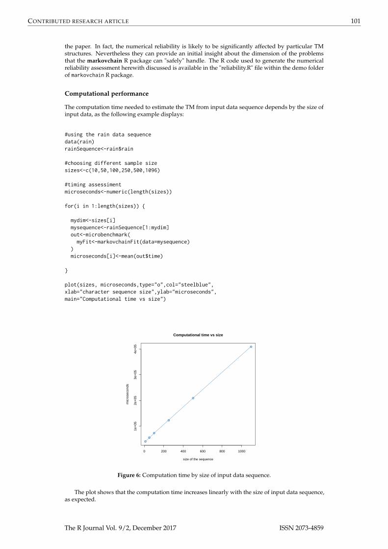
The computation time needed to estimate the TM from input data sequence depends by the size ofinput data, as the following example displays:

#using the rain data sequencedata(rain)rainSequence<-rain$rain

#choosing different sample sizesizes<-c(10,50,100,250,500,1096)

#timing assessimentmicroseconds<-numeric(length(sizes))

for(i in 1:length(sizes)) {

mydim<-sizes[i]mysequence<-rainSequence[1:mydim]out<-microbenchmark(myFit<-markovchainFit(data=mysequence)

)microseconds[i]<-mean(out$time)

}

plot(sizes, microseconds,type="o",col="steelblue",xlab="character sequence size",ylab="microseconds",main="Computational time vs size")

●

●

●

●

●

●

0 200 400 600 800 1000

1e+

052e

+05

3e+

054e

+05

Computational time vs size

size of the sequence

mic

rose

cond

s

Figure 6: Computation time by size of input data sequence.

The plot shows that the computation time increases linearly with the size of input data sequence,as expected.

The R Journal Vol. 9/2, December 2017 ISSN 2073-4859

CONTRIBUTED RESEARCH ARTICLE 102

The last numeric example presented in the section discussing NHDTMCs shows the computationaladvantages of rewriting the kernel of core functions using Rcpp and RcppParallel snippets generatedby (Allaire et al., 2016). The rmarkovchain function allows the final user to choose whether to use theC++ implementation and a parallel backend, by setting the boolean parameters useRcpp and parallelrespectively.

microbenchmark(rmarkovchain(n=100,object=nhmcFit$estimate,what = "matrix",useRCpp = F),rmarkovchain(n=100,object=nhmcFit$estimate,what = "matrix",useRCpp = T,parallel = F),rmarkovchain(n=100,object=nhmcFit$estimate,what = "matrix",useRCpp = T,parallel = T))

The omitted output of the code snippet shown above demonstrates that the joint use of Rcpp andRcppParallel fastens the simulations around 10x with respect to the pure R sequential implementation.

Conclusions, discussion and acknowledgements

The markovchain package has been designed in order to make common operations on DTMCs aseasy as possible for statisticians. The package allows to create, manipulate, import and export DTMCs.Further, the author believes that the current version of the package fully satisfies standard needs suchas inference of underlying TM from empirical data, and states classification of a given DTMC.

The author believes that no other R package provides a set of classes, methods, and functions aswide as the one provided in markovchain, as of May 2017.

The package’s main vignette gives a complete descriptions of its capabilities, including bayesianestimation, statistical tests, classes and methods for continuous time MCs. Also, a separate vignettedescribes the functions designed to deal with higher order and multivariate MCs, and should still beconsidered experimental. In fact, such techniques are generally less used than standard DTMCs, andconsequently much less literature, applied examples, and coded algorithms are available.

Clearly, an expanded version of the package’s capabilities in that area is expected to be re-leased in the future. Current development efforts target optimizing computation speed and reli-ability, and increasing the analysis capabilities regarding statistical inference. Rewriting core func-tions using Rcpp gave a major boost in terms of computing speed, as exemplified in previous sec-tions. Moreover, the rewriting of the internal core parts of the code affected many functions, suchas markovchainFit and markovchainFitList. Feedbacks provided by the users of the package athttps://github.com/spedygiorgio/markovchain/issues have been extremely useful for improvingthe package. To illustrate, bugs due to numerical issues have been found when analyzing relativelybig MCs and have led to revising the steadyStates function to be computationally more robust. Aknown limitation of the package is the lack of a deep assessment of the performance of the package’sroutines for a relatively large TM. In fact, improving the numerical reliability of the package for largeDTMCs is an area on which efforts will be certainly allocated in the near future. At this regard, theimplementation of numerical methods methods shown in Stewart (1994) will be explored.

Finally, the package has been available on CRAN since Summer 2013. Notably, it has been granteda funding slot in both 2015, 2016 and 2017 Google Summer of Code (GSOC) editions. In particular,during 2015 GSOC a material part of R code has been ported in Rcpp coding, yielding considerablefastening in computational time. The author is extremely grateful to Tae Seung Kang, Sai BhargavYalamanchi and Deepak Yadav for their contribution in improving the package. A special thankshould be given to the RJournal referees for their constructive comments.

Giorgio Alfredo SpedicatoUnipolSai AssicurazioniPiazza della Costituzione 2Bologna 40128, Italyspedicato_giorgio@yahoo.it

Bibliography

J. Allaire, R. Francois, K. Ushey, G. Vandenbrouck, M. Geelnard, and Intel. RcppParallel: ParallelProgramming Tools for Rcpp, 2016. URL https://CRAN.R-project.org/package=RcppParallel. Rpackage version 4.3.20. [p102]

The R Journal Vol. 9/2, December 2017 ISSN 2073-4859

CONTRIBUTED RESEARCH ARTICLE 103

Antoine Filipovi, C., Pierucci, Kevin, Zarca, and Isabelle Durand-Zaleski. Markov models for healtheconomic evaluation: The r package heemod. ArXiv e-prints, 2017. URL https://pierucci.org/heemod. R package version 0.9.0. [p85]

Artur Araújo, Luís Meira-Machado, and Javier Roca-Pardiñas. TPmsm: Estimation of the transitionprobabilities in 3-state models. Journal of Statistical Software, 62(4):1–29, 2014. URL http://www.jstatsoft.org/v62/i04/. [p85]

D. Bates and M. Maechler. Matrix: Sparse and Dense Matrix Classes and Methods, 2016. URL http://CRAN.R-project.org/package=Matrix. R package version 1.2-6. [p87]

Bessi, Alessandro. MCTM: Markov Chains Transition Matrices, 2015. URL http://CRAN.R-project.org/package=MCTM. R package version 1.0. [p84]

Brémaud, Pierre. Discrete-Time Markov Models. Springer-Verlag, 1999. [p90]

C. G. Cassandras. Discrete Event Systems: Modeling and Performance Analysis. CRC, 1993. [p85]

Chambers, J.M. Software for Data Analysis: Programming with R. Statistics and computing. Springer-Verlag, 2008. ISBN 9780387759357. [p87]

W.-K. Ching, M. K. Ng, and E. S. Fung. Higher-order multivariate markov chains and their applications.Linear Algebra and its Applications, 428(2):492–507, 2008. [p84]

B. A. Craig and P. P. Sendi. Estimation of the transition matrix of a discrete-time markov chain. HealthEconomics, 11(1), 2002. [p84]

Csardi, Gabor and Nepusz, Tamas. The igraph software package for complex network research.InterJournal, Complex Systems:1695, 2006. URL http://igraph.sf.net. [p87]

Eddelbuettel, Dirk. Seamless R and C++ Integration with Rcpp. Springer-Verlag, New York, 2013. ISBN978-1-4614-6867-7. [p87]

Efron, B. Bootstrap methods: Another look at the jackknife. Ann. Statist., 7(1):1–26, 1979. URLhttp://dx.doi.org/10.1214/aos/1176344552. [p96]

Feres, Renaldo. Notes for math 450 matlab listings for markov chains, 2007. URL http://www.math.wustl.edu/~feres/Math450Lect04.pdf. [p90]

V. Goulet, C. Dutang, M. Maechler, D. Firth, M. Shapira, M. Stadelmann, and expm-developers@lists.R-forge.R-project.org. Expm: Matrix Exponential, 2015. URL http://CRAN.R-project.org/package=expm. R package version 0.999-0. [p87, 89]

C. M. Grinstead and J. L. Snell. Introduction to Probability. American Mathematical Soc., 2012. [p85]

L. Himmelmann. HMM: HMM - Hidden Markov Models, 2010. URL https://CRAN.R-project.org/package=HMM. R package version 1.0. [p85]

C. H. Jackson. Multi-state models for panel data: The msm package for r. Journal of Statistical Software,38(8):1–29, 2011. URL http://www.jstatsoft.org/v38/i08/. [p85]

J. Jarvis and D. R. Shier. Graph-theoretic analysis of finite markov chains. Applied mathematical modeling:a multidisciplinary approach, 1999. [p85]

C. I. Jones. On the evolution of the world income distribution. Available at SSRN 59412, 1997. [p84]

J. G. Kemeny, J. L. Snell, and G. L. Thompson. Finite mathematics. DC Murdoch, Linear Algebra forUndergraduates, 1974. [p85]

Lawrence Page, Sergey Brin, Rajeev Motwani, and Terry Winograd. The pagerank citation ranking:Bringing order to the web. Technical Report 1999-66, Stanford InfoLab, 1999. URL http://ilpubs.stanford.edu:8090/422/. Previous number = SIDL-WP-1999-0120. [p84]

A. A. Markov. Issledovanie zamechatel nogo sluchaya zavisimyh ispytanij. Izvestiya Akademii Nauk,SPb, VI seriya, 1(93):61–80, 1907. [p84]

MATLAB. Version 9.2.0 (R2017a). The MathWorks Inc., Natick, Massachusetts, 2017. [p85]

Montgomery, James. Communication classes, 2009. URL http://www.ssc.wisc.edu/~jmontgom/commclasses.pdf. [p90]

The R Journal Vol. 9/2, December 2017 ISSN 2073-4859

CONTRIBUTED RESEARCH ARTICLE 104

Nicholson, William. DTMCPack: Suite of Functions Related to Discrete-Time Discrete-State Markov Chains,2013. URL http://CRAN.R-project.org/package=DTMCPack. R package version 0.1-2. [p84]

Pablo J. Villacorta and José L. Verdegay. FuzzyStatProb: An r package for the estimation of fuzzystationary probabilities from a sequence of observations of an unknown Markov chain. Journal ofStatistical Software, 71(8):1–27, 2016. URL https://doi.org/10.18637/jss.v071.i08. [p85]

P. Roebuck. Matlab: MATLAB Emulation Package, 2014. URL http://CRAN.R-project.org/package=matlab. R package version 1.0.2. [p87]

M. Scholz. The R package clickstream: Analyzing clickstream data with markov chains. Journal ofStatistical Software, 74(4):1–17, 2016. URL https://doi.org/10.18637/jss.v074.i04. [p84]

Spedicato, Giorgio Alfredo. markovchain: An R Package to Easily Handle Discrete Markov Chains, 2016.R package version 0.6.5. [p84]

W. J. Stewart. Introduction to the Numerical Solutions of Markov Chains. Princeton Univ. Press, 1994.[p102]

I. Visser and M. Speekenbrink. depmixS4: An r package for hidden markov models. Journal ofStatistical Software, 36(7):1–21, 2010. URL http://www.jstatsoft.org/v36/i07/. [p85]

Wolfram Research, Inc. Mathematica. Wolfram Research, Inc., ninth edition, 2013. [p85]

The R Journal Vol. 9/2, December 2017 ISSN 2073-4859