discrete-time signals & systems -...
TRANSCRIPT
Discrete-time Signals & SystemsFrequency Analysis of Discrete-Time Signals
S Wongsa
11
S Wongsa
Dept. of Control Systems and Instrumentation Engineering,
KMUTT
Overview
Discrete-time processing of continuous-time signals
Time & Frequency Domain
Sampling Theorem
Aliasing
Frequency Analysis of Discrete-Time Signals
22
DTFT
DFT
Frequency Analysis of Discrete-Time Signals
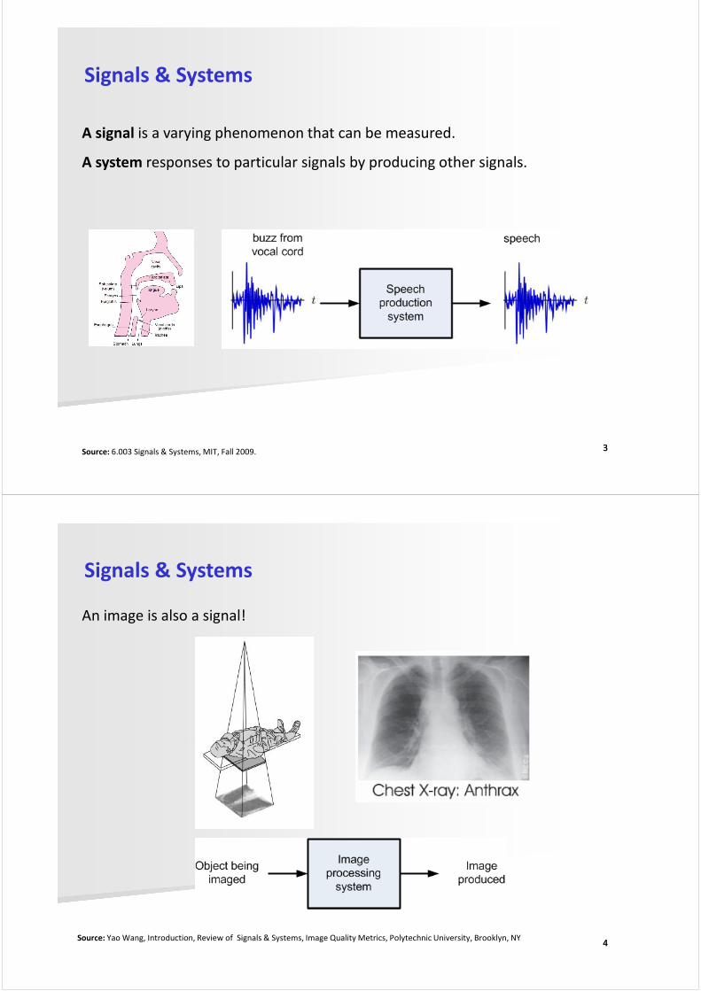
Signals & Systems
A signal is a varying phenomenon that can be measured.
A system responses to particular signals by producing other signals.
33Source: 6.003 Signals & Systems, MIT, Fall 2009.
Signals & Systems
An image is also a signal!
44Source: Yao Wang, Introduction, Review of Signals & Systems, Image Quality Metrics, Polytechnic University, Brooklyn, NY
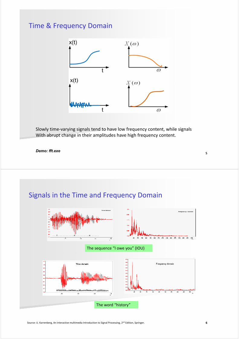
Time & Frequency Domain
55
Slowly time-varying signals tend to have low frequency content, while signals
With abrupt change in their amplitudes have high frequency content.
Demo: fft.exe
Signals in the Time and Frequency Domain
The sequence “I owe you” (IOU)
66Source: U. Karrenberg, An interactive multimedia Introduction to Signal Processing, 2nd Edition, Springer.
The word “history”
Signals in the Time and Frequency Domain
77
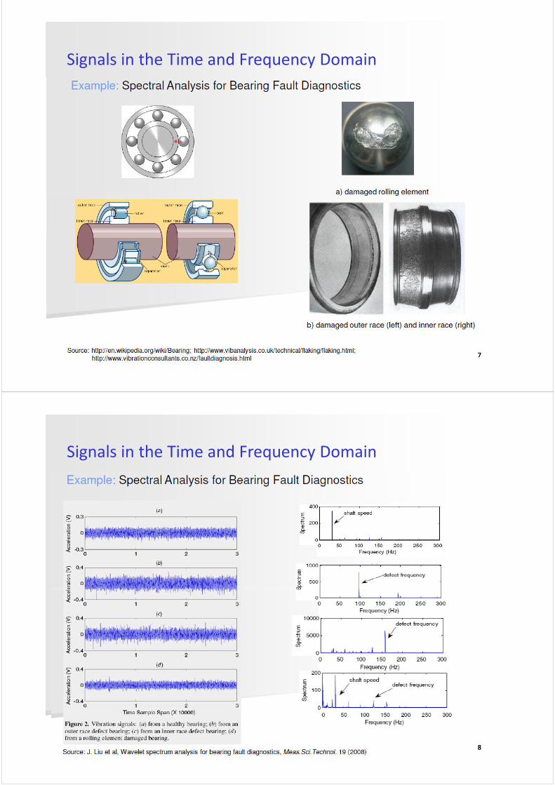
Signals in the Time and Frequency Domain
88
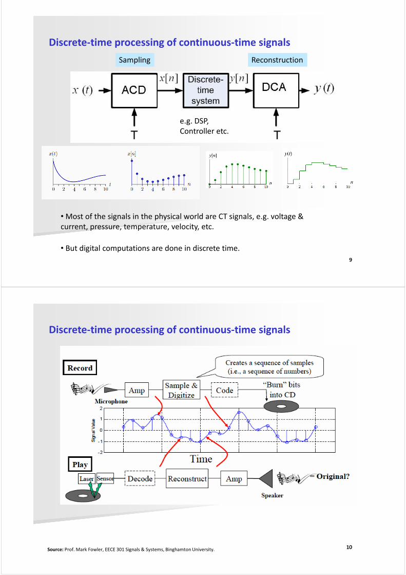
Discrete-time processing of continuous-time signals
Sampling Reconstruction
e.g. DSP,
Controller etc.
99
• Most of the signals in the physical world are CT signals, e.g. voltage &
current, pressure, temperature, velocity, etc.
• But digital computations are done in discrete time.
Discrete-time processing of continuous-time signals
1010Source: Prof. Mark Fowler, EECE 301 Signals & Systems, Binghamton University.
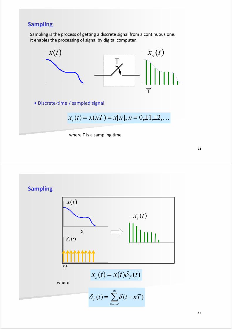
Sampling
Sampling is the process of getting a discrete signal from a continuous one.
It enables the processing of signal by digital computer.
T
)(tx )(txs
1111
• Discrete-time / sampled signal
K,2,1,0 ],[)()( ±±=== nnxnTxtxs
T
where T is a sampling time.
Sampling
)(tx
)(txs
)(tTδX
1212
)()()( ttxtx Ts δ=where
∑∞
−∞=
−=n
T nTtt )()( δδ
T
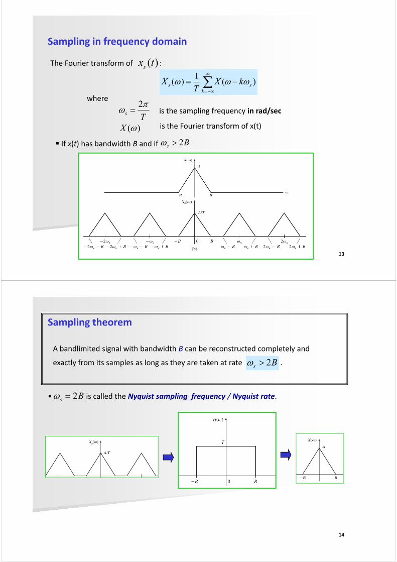
Sampling in frequency domain
The Fourier transform of : )(txs
∑∞
−∞=
−=k
ss kXT
X )(1
)( ωωω
where
Ts
πω
2= is the sampling frequency in rad/sec
If x(t) has bandwidth B and if B2>ω
)(ωX is the Fourier transform of x(t)
1313
If x(t) has bandwidth B and if Bs 2>ω
Sampling theorem
A bandlimited signal with bandwidth B can be reconstructed completely and
exactly from its samples as long as they are taken at rate .Bs 2>ω
• is called the Nyquist sampling frequency / Nyquist rate.Bs 2=ω
1414
Aliasing
Q : What if the signal is not bandlimited nor is the sampling frequency greater
than the Nyquist sampling frequency?
A : The high frequency components of x(t) will be transposed to low-frequency
components, leading to a phenomenon called aliasing.
1515
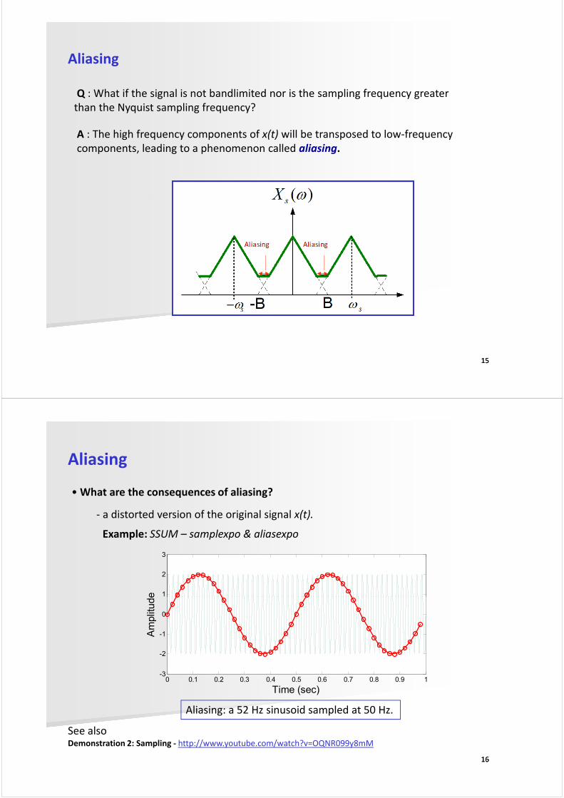
Aliasing
• What are the consequences of aliasing?
- a distorted version of the original signal x(t).
Example: SSUM – samplexpo & aliasexpo
1
2
3
Amplitude
1616
See also Demonstration 2: Sampling - http://www.youtube.com/watch?v=OQNR099y8mM
0 0.1 0.2 0.3 0.4 0.5 0.6 0.7 0.8 0.9 1-3
-2
-1
0
1
Time (sec)
Amplitude
Aliasing: a 52 Hz sinusoid sampled at 50 Hz.
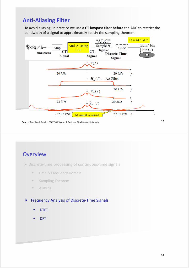
Anti-Aliasing Filter
To avoid aliasing, in practice we use a CT lowpass filter before the ADC to restrict the
bandwidth of a signal to approximately satisfy the sampling theorem.
Fs = 44.1 kHz
1717Source: Prof. Mark Fowler, EECE 301 Signals & Systems, Binghamton University.
Overview
Discrete-time processing of continuous-time signals
Time & Frequency Domain
Sampling Theorem
Aliasing
Frequency Analysis of Discrete-Time Signals
1818
DTFT
DFT
Frequency Analysis of Discrete-Time Signals
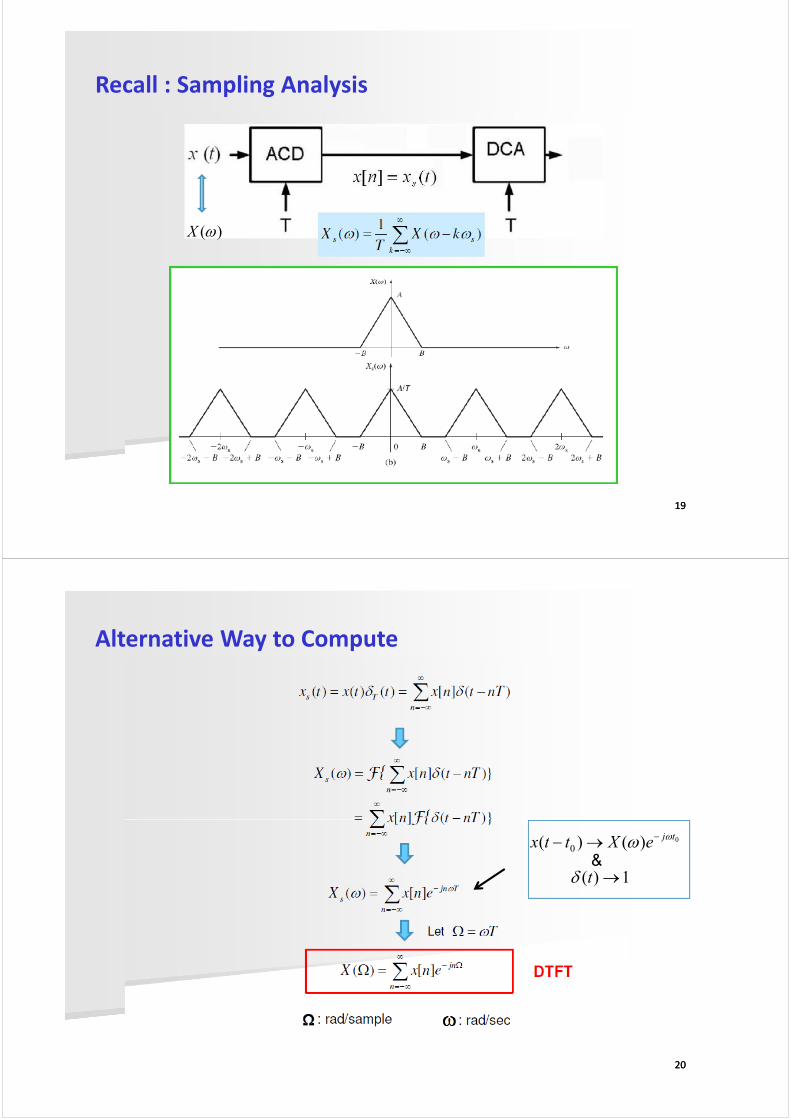
Recall : Sampling Analysis
)(ωX
1919
Alternative Way to Compute
0)()(tj
eXttxωω −→−
2020
0)()( 0
tjeXttx
ωω −→−
1)( →tδ&
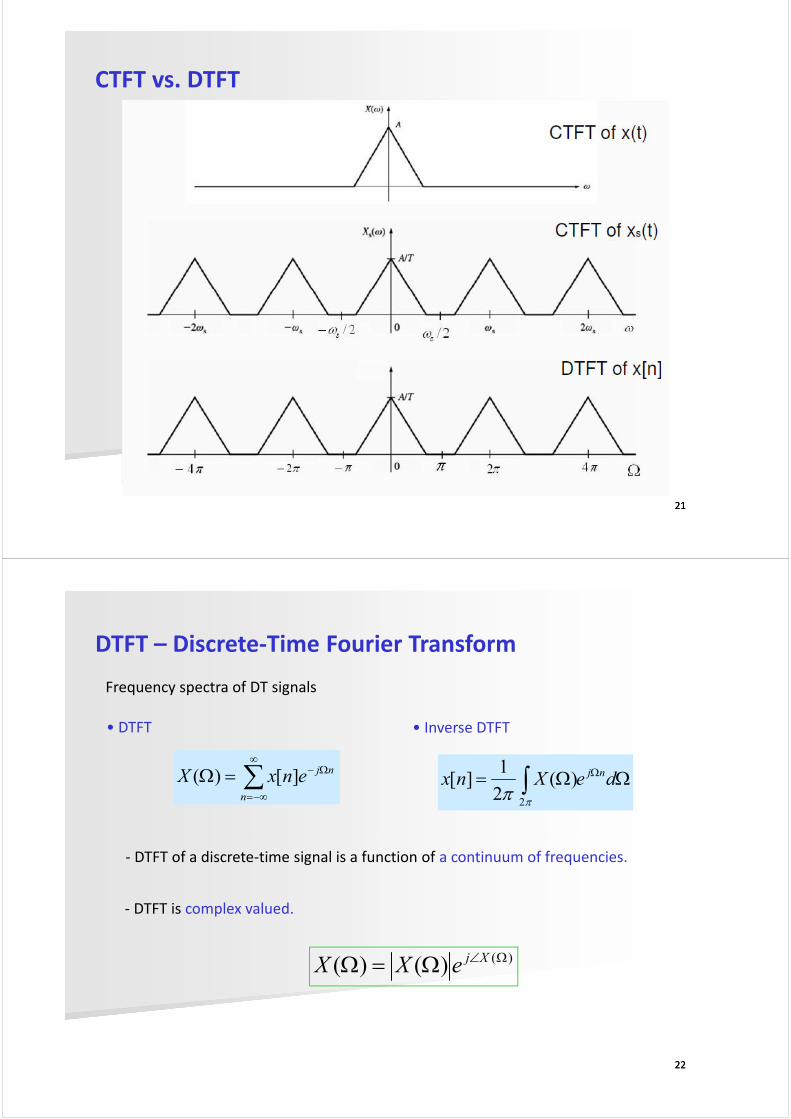
CTFT vs. DTFT
2121
DTFT – Discrete-Time Fourier Transform
Frequency spectra of DT signals
• DTFT
∑∞
−∞=
Ω−=Ωn
njenxX ][)(
• Inverse DTFT
ΩΩ= Ω∫ deXnx nj
ππ2
)(2
1][
2222
- DTFT of a discrete-time signal is a function of a continuum of frequencies.
- DTFT is complex valued.
)()()( Ω∠Ω=Ω XjeXX

DTFT – Discrete-Time Fourier Transform
Periodicity: DTFT is a periodic function of Ωwith period of 2π.
Symmetry: By replacing Ω by -Ω we can see that
)(][)( Ω==Ω− ∑∞
Ω XenxX nj
2323
)(][)( Ω==Ω− ∑−∞=
Ω XenxXn
nj
Even symmetry of |X(Ω)|
Odd symmetry of ∠X(Ω)
It is sufficient to consider the DTFT over only Ω=[0 π].
DTFT
EXAMPLE: DTFT of an exponential function
][5.0][ nunx n= n
n
j
n
njn eeX )5.0(5.0)(00
∑∑∞
=
Ω−∞
=
Ω− ==Ω
r
rrr
qqq
qn
n
−−
=+
=∑
1
1212
1
+Ω−−=Ω
qjeX
)5.0(1lim)(
12
2424
Ω−∞→ −−
=Ωjq
e
eX
5.01
)5.0(1lim)(
2
Ω−−=Ω
jeX
5.01
1)(
π/ΩNB: Normalized frequency = radians/unit time
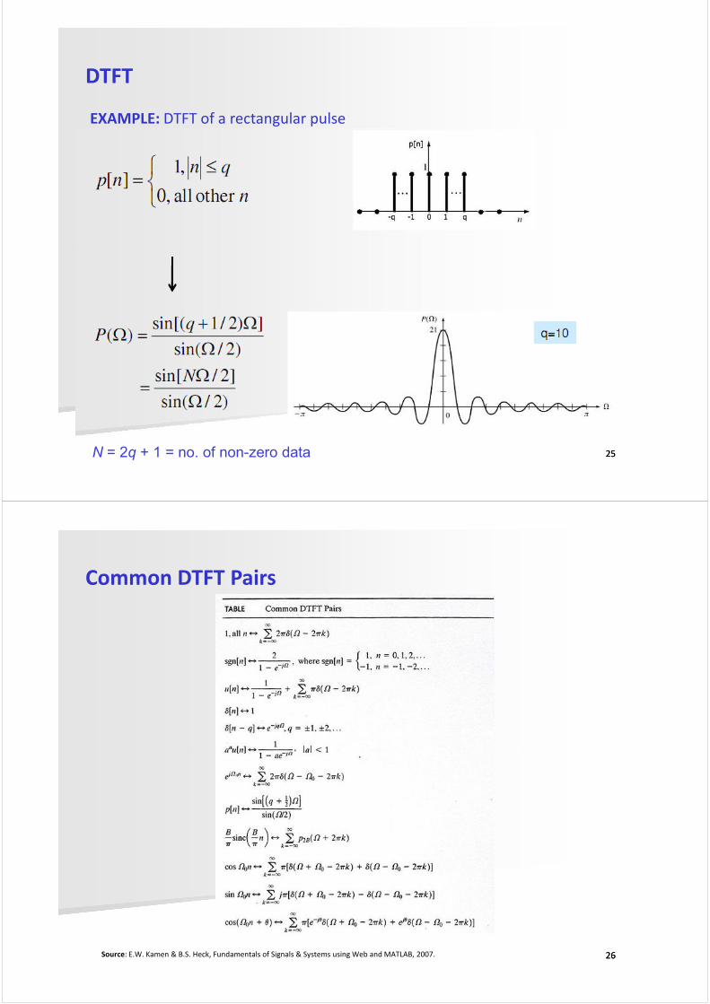
DTFT
EXAMPLE: DTFT of a rectangular pulse
2525N = 2q + 1 = no. of non-zero data
Common DTFT Pairs
2626Source: E.W. Kamen & B.S. Heck, Fundamentals of Signals & Systems using Web and MATLAB, 2007.
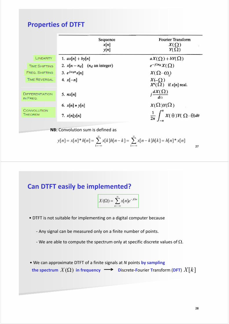
Properties of DTFT
2727
NB: Convolution sum is defined as
][*][][][][][][*][][ nxnhkhknxknhkxnhnxnykk
=−=−== ∑∑∞
−∞=
∞
−∞=
Can DTFT easily be implemented?
• DTFT is not suitable for implementing on a digital computer because
- Any signal can be measured only on a finite number of points.
- We are able to compute the spectrum only at specific discrete values of Ω.
∑∞
−∞=
Ω−=Ωn
njenxX ][)(
2828
- We are able to compute the spectrum only at specific discrete values of Ω.
• We can approximate DTFT of a finite signals at N points by sampling
the spectrum in frequency Discrete-Fourier Transform (DFT))(ΩX ][kX
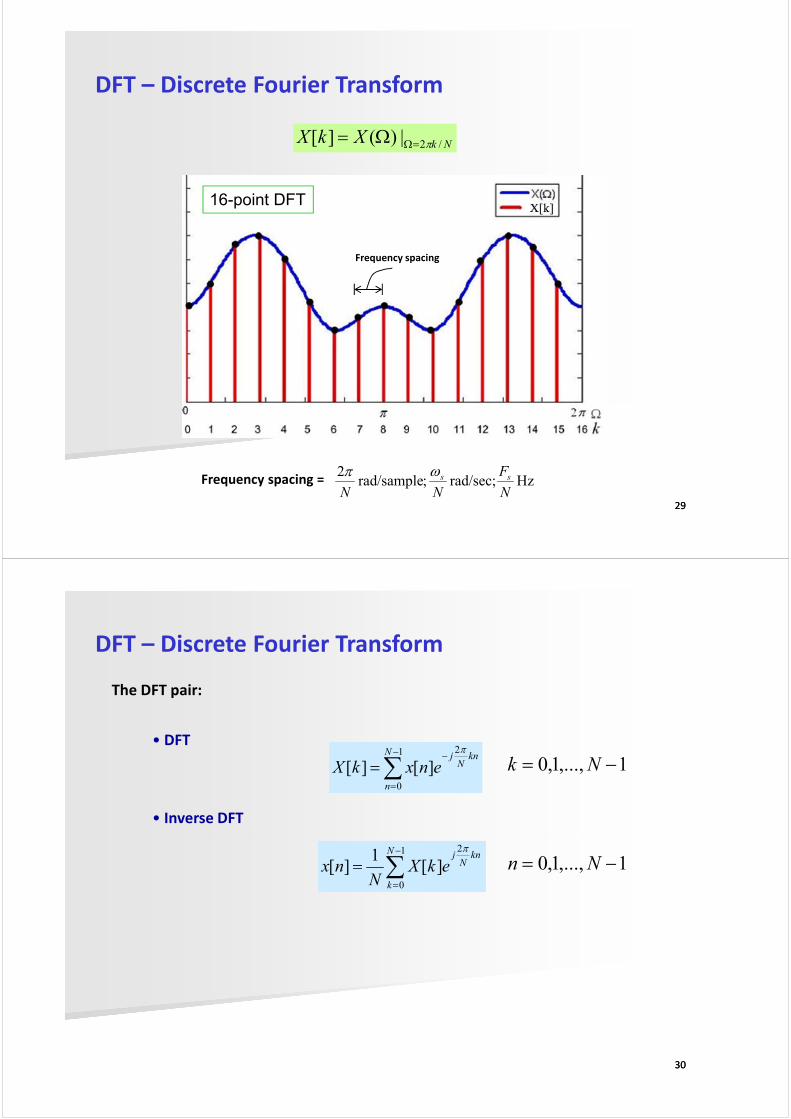
DFT – Discrete Fourier Transform
NkXkX /2|)(][ π=ΩΩ=
16-point DFT
Frequency spacing
2929
Hz rad/sec; ;rad/sample 2
N
F
NN
ssωπFrequency spacing =
DFT – Discrete Fourier Transform
The DFT pair:
• DFT
∑−
=
−=
1
0
2
][][N
n
knNj
enxkX
π
• Inverse DFT
1,...,1,0 −= Nk
3030
∑−
=
=1
0
2
][1
][N
k
knNj
ekXN
nx
π
1,...,1,0 −= Nn
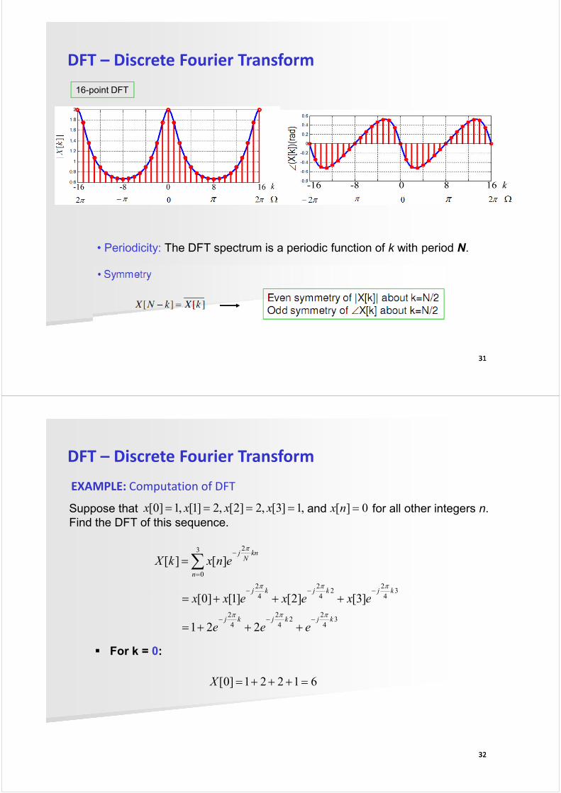
DFT – Discrete Fourier Transform
16-point DFT
3131
• Periodicity: The DFT spectrum is a periodic function of k with period N.
DFT – Discrete Fourier Transform
EXAMPLE: Computation of DFT
Suppose that and for all other integers n.
Find the DFT of this sequence.
,1]3[,2]2[,2]1[,1]0[ ==== xxxx 0][ =nx
34
22
4
2
4
2
3
0
2
]3[]2[]1[]0[
][][
kjkjkj
n
knNj
exexexx
enxkX
πππ
π
−−−
=
−
+++=
=∑
3232
34
22
4
2
4
2
34
244
221
]3[]2[]1[]0[
kjkjkj
kjkjkj
eee
exexexx
πππ−−−
−−−
+++=
+++=
For k = 0:
61221 ]0[ =+++=X
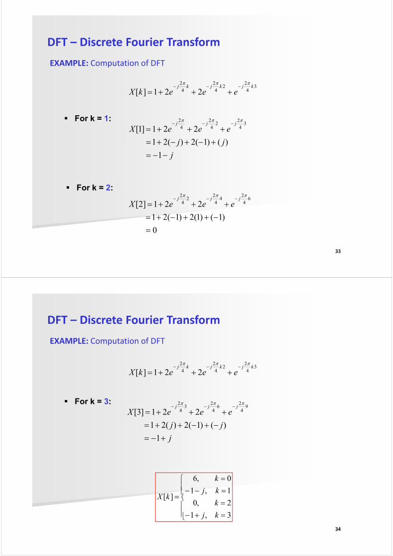
DFT – Discrete Fourier Transform
EXAMPLE: Computation of DFT
34
22
4
2
4
2
221 ][kjkjkj
eeekXπππ
−−−+++=
For k = 1:
jj
eeeXjjj
+−+−+=
+++=−−−
)()1(2)(21
221]1[3
4
22
4
2
4
2 πππ
3333
j
jj
−−=
+−+−+=
1
)()1(2)(21
For k = 2:
0
)1()1(2)1(21
221]2[6
4
24
4
22
4
2
=
−++−+=
+++=−−−
πππjjj
eeeX
DFT – Discrete Fourier Transform
EXAMPLE: Computation of DFT
34
22
4
2
4
2
221 ][kjkjkj
eeekXπππ
−−−+++=
For k = 3:
eeeXjjj
+++=−−−
221]3[9
4
26
4
23
4
2 πππ
3434
j
jj
eeeX
+−=
−+−++=
+++=
1
)()1(2)(21
221]3[
=+−
=
=−−
=
=
3,1
2,0
1,1
0,6
][
kj
k
kj
k
kX
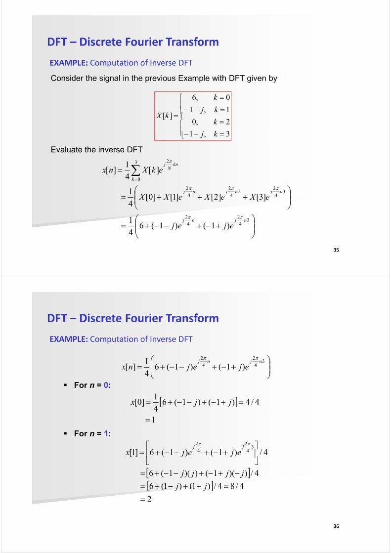
DFT – Discrete Fourier Transform
EXAMPLE: Computation of Inverse DFT
=+−
=
=−−
=
=
3,1
2,0
1,1
0,6
][
kj
k
kj
k
kX
Consider the signal in the previous Example with DFT given by
3535
=+− 3,1 kj
Evaluate the inverse DFT
+−+−−+=
+++=
= ∑=
34
2
4
2
34
22
4
2
4
2
3
0
2
)1()1(6 4
1
]3[]2[]1[]0[4
1
][4
1][
njnj
njnjnj
k
knNj
ejej
eXeXeXX
ekXnx
ππ
πππ
π
DFT – Discrete Fourier Transform
EXAMPLE: Computation of Inverse DFT
+−+−−+=
34
2
4
2
)1()1(64
1 ][
njnj
ejejnxππ
For n = 0:
[ ] 4/4)1()1(6 4
1]0[
=
=+−+−−+= jjx
3636
1 =
For n = 1:
[ ][ ]2
4/84/)1()1(6
4/))(1())(1(6
4/)1()1(6 ]1[3
4
2
4
2
=
=++−+=
−+−+−−+=
+−+−−+=
jj
jjjj
ejejxjj
ππ
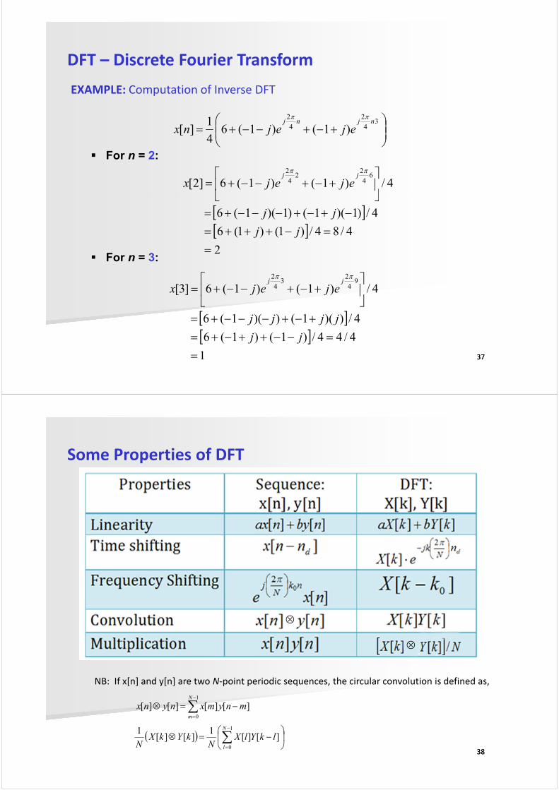
DFT – Discrete Fourier Transform
EXAMPLE: Computation of Inverse DFT
+−+−−+=
34
2
4
2
)1()1(64
1 ][
njnj
ejejnx
ππ
For n = 2:
4/)1()1(6 ]2[6
4
22
4
2
+−+−−+= ejejx
jjππ
3737
For n = 3:
[ ][ ]1
4/44/)1()1(6
4/))(1())(1(6
4/)1()1(6 ]3[9
4
23
4
2
=
=−−++−+=
+−+−−−+=
+−+−−+=
jj
jjjj
ejejxjj
ππ
[ ][ ]2
4/84/)1()1(6
4/)1)(1()1)(1(6
=
=−+++=
−+−+−−−+=
jj
jj
Some Properties of DFT
3838
NB: If x[n] and y[n] are two N-point periodic sequences, the circular convolution is defined as,
∑−
=
−=⊗1
0
][][][][N
m
mnymxnynx
( )
−=⊗ ∑
−
=
1
0
][][1
][][1 N
l
lkYlXN
kYkXN
⊗
⊗
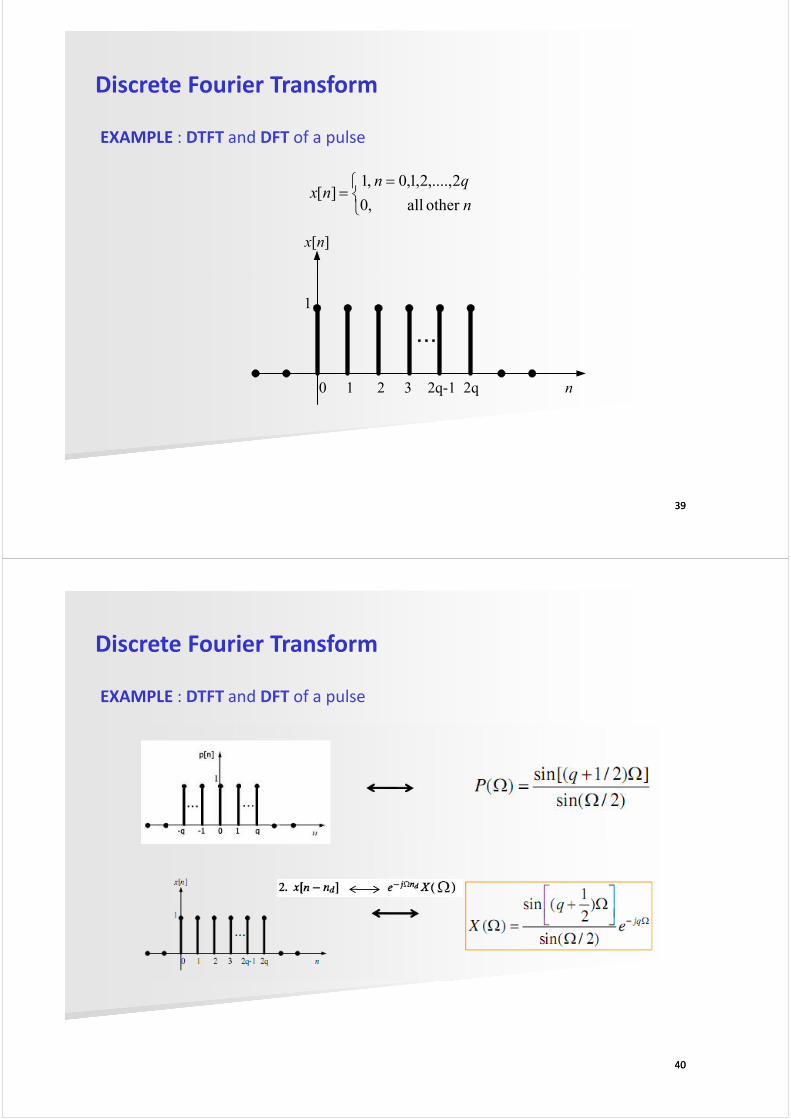
Discrete Fourier Transform
=
=n
qnnx
other all ,0
2,....,2,1,0 ,1][
x[n]
EXAMPLE : DTFT and DFT of a pulse
3939
...
0 1 2 3 2q-1 2q n
1
Discrete Fourier Transform
EXAMPLE : DTFT and DFT of a pulse
4040
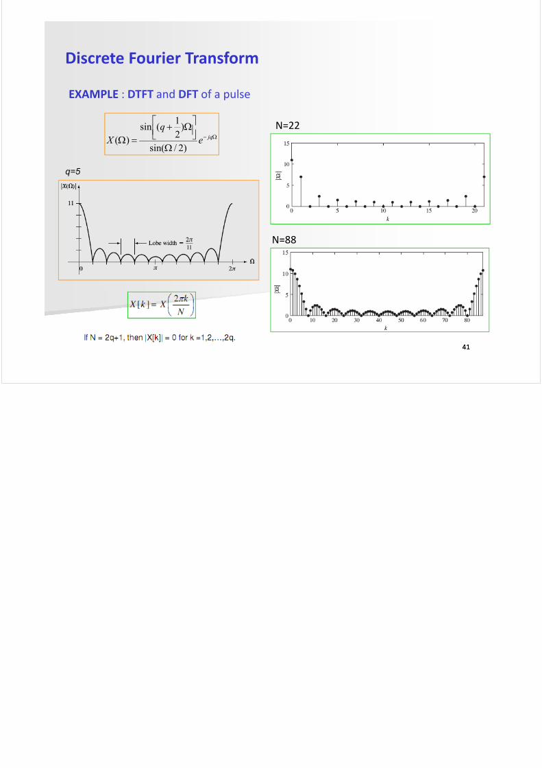
Discrete Fourier Transform
EXAMPLE : DTFT and DFT of a pulse
N=22Ω−
Ω
Ω+=Ω jqe
q
X)2/sin(
)2
1(sin
)(
q=5
4141
N=88