Discrimination in Auctions for Renewable Energy Support:

Three Theoretically Equivalent but Practically Different

Concepts

Karl-Martin Ehrhart1,1, Marie-Christin Haufe1,1, Jan Kreiss1,1,

aTakon GmbH, GermanybKarlsruhe Institute of Technology (KIT), Germany

Abstract

The design of auctions for renewable energy support becomes more complex by the in-

tegration of different types of bidder into the same auction. This particularly applies to

auctions in which bidders with asymmetric cost structures participate, e.g., bidders with

different technologies in technology-neutral auctions or bidders from different countries

in cross-border auctions. In order to privilege specific bidder groups and to control the

allocation, discriminatory elements are included into the auction design. We analyze

the three most applied discriminatory instruments: a minimum quota or a bonus for

a bidder class to be privileged or different maximum prices for different bidder classes.

Typically, these instruments discriminate stronger bidders (with lower costs) in favor of

weaker bidders (with higher costs). We show that all three instruments can reduce the

support costs in comparison to free competition by applying the principle of monopolis-

tic third-degree price discrimination. Moreover, we prove that the three instruments are

theoretically equivalent: every auction outcome that can be reached by one instrument

can also be reached by the others including the outcome with minimal support costs.

However, there are crucial differences concerning the practical application, particularly

∗Corresponding authorEmail addresses: ehrhart@kit.edu (Karl-Martin Ehrhart), haufe@takon.com (Marie-Christin

Haufe), kreiss@takon.com (Jan Kreiss)

1

with respect to the robustness to misestimations of the cost structures. We show that

the combination of the instruments helps to avoid costly errors. Finally, we illustrate

our analyses by an example.

1. Introduction

Competitive bidding processes are globally becoming the instrument of choice re-

garding the promotion of renewable energies (RE). Auctions have proven to reduce the

costs of RE support, increase efficiency, and control the RE expansion in order to reach

the respective targets (Wigand et al, 2016). Therefore, the European Commission re-

quires its member states from 2017 on to conduct auctions for RE support (European

Commission, 2014). Moreover, the European Commission also proposes to conduct

auctions that are open to multiple RE technologies. This requirement is based on the

assumption that multi-technology auctions increase efficiency and reduce support costs

even further.1 Multi-technology auctions have been implemented, e.g., in the United

Kingdom (Department for Business, Energy & Industrial Strategy, 2017), Spain (Min-

isterio de Energia, Turismo y Agenda Digital, 2017a), the Netherlands (Minister van

Economische Zaken, 2015) or Mexico (Centro Nacional de Control de Energia, 2017).

Denmark and Germany conducted auctions for large PV installations that were open

to bidders from both countries (Kitzing and Wendring, 2016).

Although there is a vast consensus about the use of auctions for RE support, national

governments pursue different targets with their auctions, particularly with respect to the

type of costs that are aimed to be minimized (Kreiss et al, 2017). There are arguments

to address only support costs or only generation costs or also to include integration costs

(Joskow, 2011; Ueckerdt et al, 2013). Most commonly, the minimization of support costs

1Concerns about windfall profits are sometimes cited as arguments against auctions with heteroge-nous types of bidders, e.g., multi-technology auctions (Held et al, 2006).

2

is the stated primary goal and main reason for RE auctions, e.g., in the United Kingdom

(Department of Energy and Climate Change, 2011), in Mexico (Centro Nacional de

Control de Energia, 2017) and in California (Public Utilities Commission of the State

of California, 2010) it is explicitly stated that the auctions should minimize the costs of

RE support. The definition of auction goals in other countries and even the statement

of the European Commission can be interpreted so that the support costs are (one

of) the most important target (European Commission, 2014; Ministerio de Energia,

Turismo y Agenda Digital, 2017b). That is, the minimization of support costs attracts

particular attentions when designing auctions for RE support.

Auctions for RE support also include discriminatory design elements to privilege

specific bidder groups and to control the allocation. The focus of this paper is to

analyze different discriminatory instruments and their effects on the auction outcome,

particularly on support costs. The considered instruments are minimum or maximum

quotas, maximum prices (i.e., reservation prices), and boni or mali for different bidder

classes. All these instruments have been implemented in auctions for RE support:

different maximum prices in the multi-technology auction in the Netherlands (Minister

van Economische Zaken, 2015), a bonus depending on the location in the German

auction for onshore wind (Deutscher Bundestag, 2016) and quotas that depend on the

availability in the Californian auctions (Public Utilities Commission of the State of

California, 2010).

The implementation of discriminatory instruments is often not only intensified by

the minimization of the support costs but also by other criteria, e.g., grid and system

integration, mixture of different RE technologies, regional distribution of RE, or actor

diversity (Kreiss et al, 2017). Also in the context of such criteria, it is important to

understand the effects of the discriminatory instruments on the auction outcome and

the support costs.

3

The effects of discriminatory instruments implemented in markets and especially in

auctions have been theoretically analyzed in a general context by, e.g., Schmalensee

(1981), Varian (1989), Myerson (1981), Bulow and Roberts (1989), and McAfee and

McMillan (1989). This paper goes one step further with a detailed analysis of the three

discriminatory instruments for the actual application of RE auctions.

We show that each instrument (quota, bonus, maximum price) can reduce the sup-

port costs for RE sources, and we derive optimality conditions (w.r.t. support cost

minimization) for each instrument and prove that the instruments are theoretically

equivalent: every auction outcome (including support costs) that can be implemented

by a specific parameterization of one instrument can also be reached by the two other

(correspondingly parameterized) instruments.

However, with respect to the application in practice, there are crucial differences

between the instruments, which have to be taken into account when deciding on their

implementation and calibration. This particularly refers to the robustness of the desired

effects of discrimination and the risk and magnitude of undesired effects that may be

caused by a wrong calibration, e.g., due to misestimation of the absolute and relative

strength of the different bidder classes that are treated differently in the auction. This is

also of particular interest in the above mentioned cases with additional or other targets

than the minimization of support costs.

This paper transfers microeconomic theory to a dynamic environment of increasing

importance. It helps to understand the effects that different discriminatory instru-

ments have on bidding behavior and the auction outcome. Since auctions for RE sup-

port become increasingly relevant and more and more auctions are opened for several

technologies or participants from different countries, the relevance of this topic also

increases.

In Section 2 we introduce the framework of our theoretic analysis of auctions for RE

4

support. The discriminatory instruments of a quota, maximum price, and a bonus are

analyzed in Sections 2.1, 2.2, and 2.3. An illustrating example is provided in Section

2.4. The results of our analyses are compared and discussed regarding the practical

implementation in Section 3. We summarize in Section 4.

2. Model

Consider a procurement auction for RE support with a fixed demand D for a specific

good (e.g., capacity [MW] or energy [MWh per year]). The supply side is modeled by

single-project bidders each offering the same volume share that sum up to the total

supply. The bidders have independent and private project costs for producing an unit

of the good. The ascending order of private project costs is given by the marginal cost

function MC(x) with MC(0) > 0 and MC ′(x) = dMC(x)dx

> 0 for all x ≥ 0. That is, if

x is delivered by the projects with the lowest costs, MC(x) are the highest marginal

costs among these projects. The lowest total costs C(x) for delivering x are given by

the cumulated marginal costs, C(x) =∫ x0MC(z)dz. In the context of RE, MC(x) are

the levelized costs of electricity (LCOE) at x, i.e., the net present value of the total life

cycle costs per unit of generated electricity of the RE source which would be ranked in

the ascending order at x (Short et al, 1995). Hence, C(x) are the aggregated LCOE for

delivering x of all RE sources with LCOE lower than or equal to MC(x).

There are two disjoint classes of bidders (e.g., two different technologies): low-

cost bidders (L) and high-cost bidders (H). The two bidder classes L and H are

characterized by different marginal cost functions MCL and MCH with

MCL(x) < MCH(x) for all x ≥ 0. (1)

That is, the marginal costs and total costs for delivering any volume x are lower for

5

the low-cost bidders than for the high-cost bidders. In the context of RE, this means

that the high-cost bidders need higher support for delivering a certain volume x than

the low-cost bidders. According to IRENA (2015), different RE sources in different

countries and different years have significantly different cost structures. This means,

costs to supply RE in a specific country and year are lower for one technology than for

another. However, the overall costs might be minimized utilizing both technologies2.

In the auction, the uniform price rule is applied and the uniform price is determined

by the lowest rejected bid.3 Bidders simultaneously submit their bids for the monetary

support for their projects. In this auction, a bidder’s optimal bidding strategy (weakly

dominant strategy) is to bid the support that exactly covers his costs (Weber, 1983).

Therefore, the supply functions SL(p) and SH(p) of the low-cost and high-cost bidders

are given by

SL(p) = MC−1L (p) and SH(p) = MC−1H (p) (2)

and increase in the price p. From (1) follows

SL(p) > SH(p) for all p ≥MCL(0) . (3)

Thus, in free competition, the market clearing price p∗ is determined by

SL(p∗) + SH(p∗) = D , (4)

where the supply of the low-cost bidders exceeds the supply of the high-cost bidders:

2Even though the marginal costs for every demand x are lower for one technology, there are demandsy and y with y > y so that the marginal costs for the lower cost technology for demand y are higherthan for the higher cost technology and the lower demand y, i.e., MCH(y) < MCL(y)

3Since the marginal cost functions and, thus, the supply functions are continuous, there is nodifference between the price rule of the lowest rejected bid and the price rule of the highest acceptedbid, which is more common in practice.

6

SL(p∗) > SH(p∗) ≥ 0. The auctioneer’s total costs amount to K(p∗) = p∗D, i.e., the

overall costs of all support payments to the awarded RE projects.

The elasticities of supply of the two bidder classes L and H are defined as

εi(p) =S ′i(p)

Si(p)p with S ′i(p) =

dSi(p)

dp, i ∈ {L,H} . (5)

Additional to (1), we state the following assumptions.

Assumption 1.

(i) The elasticities of supply εL(p) and εH(p) are non-increasing in p.

(ii) SH(p∗) > 0 and εL(p∗) < εH(p∗) at the market clearing price p∗ of free competi-

tion.

Assumption (i) is a standard economic assumption and also supported by the RE

literature (de Vries et al, 2007; Hoefnagels et al, 2011; Brown et al, 2016). Assumption

(ii) is more context sensitive: the high-cost bidders at least gain a small share in a non-

discriminatory auction.4 Since this share is smaller than that of the low-cost bidders,

it is reasonable to assume that the high-cost bidders’ price elasticity of supply at p∗ is

higher than that of the low-cost bidders.

In the following, we analyze and compare three commonly discussed and imple-

mented instruments of discrimination. First, a quota is granted to the high-cost bid-

ders in order to guarantee a certain minimum amount delivered by them. Second, a

maximum (reservation) price for the low-cost bidders is set, which the low-cost bidders

4In case that the bidder classes are distinguished by their technology, there are examples of regionswhere one technology is much less costly than the other so that the high-cost bidders never have achance to be awarded in a non-discriminatory auction. This, for example applies to North Dakota(Brown et al, 2016) or to Norway (Hoefnagels et al, 2011), where wind energy is much less costly thanPV. However, there are many examples where wind and solar are both awarded in multi-technologyauctions, e.g. Mexico (IRENA, 2017), or are awarded in separate auctions but at similar price levels,e.g. in Germany (Bundesnetzagentur, 2017a,b).

7

must not exceed with their bids. Third, the high-cost bidders receive a bonus in form

of an additional payment in case of award. All three forms of discrimination induce a

(supply) volume shift from the low-cost to the high-cost bidders (by always covering

the total auction volume D) involving a respective price change. Moreover, all three

forms of discrimination necessarily involve different prices pL and pH for the awarded

low-cost and the awarded high-cost bidders.

In our analyses, we consider the total support costs

K(pL, pH) = pLSL(pL) + pHSH(pH) (6)

which depend on the prices pL and pH and the corresponding supply volumes SL(pL)

and SH(pH) with SL(pL) + SH(pH) = D.

2.1. Quota

Consider a minimum quota Q < D (sometimes referred to as minimum contingent)

for the high-cost bidders.5 The quota guarantees that the high-cost bidder group will

at least supply Q. Thus, the low-cost bidders’ supply never exceeds D−Q. The quota

only becomes effective if Q > SH(p∗), i.e., the high-cost bidders would not reach Q in

free competition. If the quota becomes effective, each bidder class gets its own uniform

award price pL and pH , which are given by

pL = MCL(D −Q) and pH = MCH(Q) . (7)

The volume shift

q = max{Q− SH(p∗), 0} (8)

5Analogously, we could consider a maximum quota for the low-cost bidders.

8

from the low-cost bidders to the high-cost bidders, induced by the quota Q, increases

the award price for the high-cost bidders and decreases the award price for the low-cost

bidders compared to free competition, pH < p∗ < pL, if q > 0. The volume shift q and

the price difference both effect the support costs. First, we investigate the effects by

starting at q = 0, which corresponds to the situation of an ineffective quota.

Lemma 1. Consider a procurement auction with uniform pricing, fixed demand D,

two bidder classes L and H and a minimum quota Q for the high-cost bidders H. The

support costs decrease when the quota becomes effective, i.e., q = max{Q − SH(p∗), 0}

becomes positive.

Lemma 1, whose proof is presented in Appendix Appendix A, states that the auc-

tioneer can reduce costs by limiting the low-cost bidders. This is due to the properties

of the elasticities of supply. If the high-cost bidders’ elasticity of supply exceeds that

of the low-cost bidders at the free competition price p∗, then the relative price change

(savings) induced by a marginal (negative) volume change for the low-cost bidder group

is greater than the relative price change (costs increase) induced by a marginal (posi-

tive) volume shift of the high-cost bidders. In other words, higher prices for the (few)

high-cost bidders increase the overall cost less than the overall cost reduction through

lower prices for the (many) low-cost bidders. Consequently, the auctioneer can reduce

the support costs by implementing a quota that leads to q > 0. Based on this result,

we prove the existence of an optimal quota and its uniqueness.

Proposition 1. There exists an unique quota Q > SH(p∗) that minimizes the support

costs. The optimal quota Q together with the award prices pL and pH are determined

by Q = SH(pH), SL(pL) + SH(pH) = D and

pH − pL =SL(pL)

S ′L(pL)− SH(pH)

S ′H(pH).

9

The proof is presented in Appendix Appendix B. The price difference pH − pL

between high-cost and low-cost bidders that is induced by the optimal quota is also

referred to in the literature. McAfee and McMillan (1989) show that this applies to

international auction where domestic and foreign companies compete. Both results are

based on the principle of monopolistic third degree price discrimination (Schmalensee,

1981; Varian, 1989). The monopolist discriminates different classes to absorb the differ-

ent spending power. In the context of auctions for RE support, the auctioneer absorbs

profits from the low-cost bidders and reduces the bidder rent at the expense of an in-

efficient outcome. The total support decreases as long as the elasticity of supply of the

high-cost bidders is larger than that of the low-cost bidders.

That is, the auctioneer not only has an incentive to implement a quota under men-

tioned conditions to reduce his costs but there also exists an optimal quota that mini-

mizes the expected support costs.

2.2. Maximum Price

The next discriminatory instrument is a reservation price r in form of a maximum

price for the low-cost bidders: low-cost bidders may not submit bids higher than r.

The maximum price does not have an effect on bidding behavior and, thus, incentive

compatibility holds: the bidders of both classes bid their true costs, except for the

low-cost bidders with higher individual costs than r, who do not participate.

The maximum price becomes effective if r < p∗, i.e., the maximum price is lower than

the uniform award price in free competition. Then, by (2), the low-cost-bidders receive

a smaller volume SL(r) < SL(p∗) and a lower price r < p∗ than in free competition

and, by (4), the high-cost bidders receive a higher volume and, by (2), a higher price.

That is, the maximum price induces a volume shift from the low-cost bidders to the

high-cost bidders and a higher price pH for the high-cost bidders than the price pL = r

for the low-cost bidders. These effects are equivalent to the effects of a volume shift (8)

10

induced by a quota Q > SH(p∗), as derived in Section 2.1.

Corollary 1. Consider a procurement auction with uniform pricing, fixed demand D,

two bidder classes L and H and a maximum price r for the low-cost bidders L.

(i) The support costs decrease when the maximum price r becomes effective, i.e., r−p∗

becomes negative.

(ii) There exists an unique maximum price r > 0 that minimizes the support costs.

The optimal maximum price r together with the award price pH for the high-cost

bidders is determined by SL(r) + SH(pH) = D and

pH − r =SL(r)

S ′L(r)− SH(pH)

S ′H(pH).

2.3. Bonus

First, we consider a bonus in form of an additional monetary payment to the awarded

high-cost bidders.6 Let b > 0 denote the bonus that is added to the award price p for

the awarded high-cost bidders.

Incentive compatibility holds in the sense that the low-cost bidders bid their true

costs and the high-cost bidders reduce their their bid by exactly the bonus b (Thiel,

1988). Thus, all bidders receive their costs if the award price equals their bid. However,

the awarded low-cost bidders receive pL = p, while the awarded high-cost bidders receive

pH = p+ b = pL + b.

The higher price pH for the high-cost bidders leads to a corresponding supply in-

crease for these bidders described by (2). Together with the analysis in Section 2.1,

this directly implies the following. First, implementing a bonus b > 0 for the high-cost

6Analogously, we could consider a malus for the low-cost bidders in form of a deduction on theaward price.

11

bidders is equivalent to a volume shift (8) from the low-cost bidders to the high-cost

bidders that is induced by a quota Q > SH(p∗). Second, the bonus that fulfills the

condition in Proposition 1, minimizes the support costs. We can state the following

result.

Corollary 2. Consider a procurement auction with uniform pricing, fixed demand D,

two bidder classes L and H and a bonus b for the high-cost bidders H.

(i) The support costs decrease when the bonus b becomes positive.

(ii) There exists an unique bonus b > 0 that minimizes the support costs. The optimal

bonus b together with the award price p is determined by SL(p) + SH(p + b) = D

and

b =SL(p)

S ′L(p)− SH(p+ b)

S ′H(p+ b).

The second bonus type is the so-called bid bonus, which reduces the high-cost

bidders’ bids by b. This reduction is only relevant in competition and does not apply

to the award price of the high-cost bidders. The bid bonus “strengthens” the bids

of the high-cost bidders and, thus, increase their chance of being awarded. Incentive

compatibility holds for both bidder classes, i.e., all bidders bid their true costs. Due

to the bid bonus, the supply of the high-cost bidders SH(pH) and their award price pH

are higher than in the free competition case, while the reverse holds for the low-cost

bidders. Since the argumentation is the same as for the monetary bonus, Corollary 2

also applies to the bid bonus.

2.4. Example

The following example illustrates the principle of functionality of the three discrim-

inatory instruments Q, bonus b and maximum price r. In our example, we assume

that the marginal costs of the bidders in class i ∈ {L,H} are uniformly distributed

12

over the interval [ai, bi] with aH > aL > 0, bH > bL, and bL > aH . We first assume

bH − aH = bL − aL and the same number of bidders in the two classes. This leads to

linear marginal cost functions of the form

MCi(x) =x

m+ ai (9)

for x ∈ [0,m(bi− ai)] with m > 0. The number of bidders is represented by m, i.e., the

inverse of the gradient of the marginal cost function, which, by assumption, is the same

in the two classes. Thus, the marginal cost functions are parallel shifts of each other.

Translated to a practical application this means that there are as many low-cost bidders

as high-cost bidders, however, there is a structural price difference (aH − aL) between

the two groups. Thus, the condition of lower costs for every quantity is fulfilled. By

(2), the supply functions for i ∈ {L,H} are

Si(p) =

0 for p < ai

m(p− ai) for p ≥ ai.

(10)

with

S ′i(p) =dSi(p)

dp= m. (11)

for p > aH , which holds by Assumption 1 (ii). By (5), the elasticity of supply is

εi(p) =S ′i(p)

Si(p)p =

p

p− ai, (12)

which is non-increasing for all p ≥ 0,

dεi(p)

dp= − ai

(p− ai)2< 0 for all p 6= ai .

13

Since aH > aL, εH(p) > εL(p) for all p > aH . In free competition, the uniform award

price p∗ is determined by the market clearing condition (4) and (10):

p∗ =D

2m+aL + aH

2.

This leads to

SH(p∗) = m(p∗ − aH) =D

2− m

2(aH − aL) ,

SL(p∗) = m(p∗ − aL) =D

2+m

2(aH − aL) .

That is, both bidder classes receive one half of the total demand plus/minus a spread

that depends on the difference (aH − aL) and the gradient m. Part (ii) of Assumption

1 requires

D

m> aH − aL . (13)

The total support costs are

K(p∗) = KL(p∗) +KH(p∗) = p∗SL(p∗) + p∗SH(p∗) = p∗m(2p∗ − aL − aH) (14)

= Dp∗ =D

2

(D

m+ aL + aH

). (15)

In Figure 1, the individual support costs KL(p∗) and KH(p∗) are visualized by the areas

p∗SL(p∗) and p∗SH(p∗). Clearly, the low-cost bidders receive a larger payment as they

supply more.

We now consider the optimal quota Q, bonus b, and maximum price r. According

to Proposition 1 and Corollary 1 and 2, optimal values of discriminatory instruments

14

SH(p∗) SL(p

∗)

p∗

Price

Quantity

MCH

MCL

Figure 1: Illustration of the example with free competition.

are determined by the price difference

pH − pL =SL(pL)

S ′L(pL)− SH(pH)

S ′H(pH)= (pL − aL)− (pH − aH) ,

which directly determines the optimal bonus b:

pH − pL =aH − aL

2= b . (16)

Applying (4), the relationship between the free competition price p∗ and the prices pH

and pL under the optimal discriminatory instruments is given by

SL(p∗) + SH(p∗) = SL(pL) + SH(pH) = D ,

⇒ 2p∗ = pH + pL .

15

With (16), we get

pH = p∗ + aH−aL4

=D

2m+

3aH + aL4

, (17)

pL = p∗ − aH−aL4

=D

2m+

3aL + aH4

= r , (18)

which also determines the optimal maximum price r.

The price increase for the high-cost bidders is equal to the price reduction for the

low-cost bidders7. By (10), (17) and (18), the supply volumes and the optimal quota

Q are

SH(pH) = m(p∗ − 3aH+aL

4

)=D

2− m

4(aH − aL) = Q , (19)

SL(pL) = m(p∗ − 3aL+aH

4

)=D

2+m

4(aH − aL) = D − Q . (20)

With (19) and (20), the volume shift q = Q− SH(p∗) from the low-cost bidders to the

high-cost bidders is

q = m

(p∗ − 3aH + aL

4

)−m(p∗ − aH) =

m

4(aH − aL) . (21)

Comparing the total support costs K(pL, pH) under the optimal quota Q, bonus b

and maximum price r with K(p∗) in free competition (14) yields

K(pL, pH) = pHSH(pH) + pLSL(pL)

=

(p∗ +

aH − aL4

)m

(p∗ − 3aH + aL

4

)+

(p∗ − aH − aL

4

)m

(p∗ − 3aL + aH

4

)= K(p∗)− m

8(aH − aL)2 < K(p∗) .

7This equality is caused by the characteristics of the example because the marginal cost curves ofboth classes are parallel shifts of each other. This equality does not necessarily hold for other marginalcost curves.

16

The support costs K(pL, pH) are lower than K(p∗) by m8

(aH − aL)2. In Figure

2, the individual support costs are visualized by the areas pHSH(pH) and pLSL(pL).

Compared to Figure 1, the sum of the two areas, i.e., the total support costs, is smaller.

Although the price increase for the high-cost bidders is equal to the price reduction

for the low-cost bidders, the overall costs for the auctioneer decrease as the number of

bidders for which the price increases is lower than the number of bidders for which the

price decreases.

Q = SH(pH) SL(pL)

r = pL

pH

Price

Quantity

MCH

MCL

b

Price

Quantity

MCH

MCL

Figure 2: Illustration of the example with optimal discriminatory instruments Q, b and r.

3. Assessment and Practical Application of the Instruments

We proved that the implementation of a quota, a bonus, or a maximum price to

discriminate the low-cost bidders in favor of the high-cost bidders reduces the overall

support costs compared to a non-discriminatory auction. The three instruments are

considered theoretically equivalent because all outcomes (including the same support

cost minimum) that can be achieved by one instrument can also be achieved by the

17

others. Moreover, the three instruments have in common that a “too aggressive” level

of discrimination may reverse the effect and increase the support costs even above the

level of a non-discriminatory auction. However, there are differences concerning the

practical implementations. In the following, we compare the three instruments with

respect to their robustness to misestimations. In Section 3.3, we extend the example of

Section 2.4 by including uncertainties regarding the marginal cost functions.

3.1. Robustness to Misestimations

As the exact number and strength of the bidders and thus their cost functions are

usually unknown to the auctioneer, he has to calibrate the discriminatory instruments

according to his beliefs and estimations. In the following, we analyze and compare

the effects of misestimations, particularly on support costs, under the three different

instruments.

Generally, a too low minimum quota for the high-cost bidders or a too high max-

imum price for the low-cost bidders may not have any effect, while a bonus is always

effective.

For a more detailed analysis, we first consider the case that the auctioneer overes-

timates the costs of the high-cost bidders, i.e., the high-cost bidders are stronger than

expected. Then, a quota does not have a negative effect because it is calibrated to

high-cost bidders which are assumed to be weaker than they actually are. The same

holds for the maximum price. In both cases, the calibration of the instrument is not

optimal, but the costs are weakly lower than in free competition. A bonus, however,

might over-privilege the high-cost bidders and, thus, increases the costs compared to

free competition. This effect becomes stronger if the anticipated high-cost bidders are

even stronger than the anticipated low-cost bidders. In this case, a quota or maximum

price are ineffective, whereas a bonus discriminates in favor of the stronger bidders and,

thus, increase the support costs.

18

Second, if the high-cost bidders’ costs are underestimated, the negative effect of

a bonus is lower than the negative effect of a quota or of a maximum price. The

bonus might not be sufficient for enough high-cost bidders to be awarded. The quota

and maximum price, however, will lead to an inappropriate share of awarded high-cost

bidders.

As a matter of course, the arguments in the last two paragraphs analogously hold

if the costs of the low-cost bidders are overestimated or underestimated. We also

discuss these two cases in the example in Section 3.3. In this section, we also analyze

the effects of a wrong estimation of the size of a bidder class, i.e., the number of

bidders within a class. In this case, a bonus is more robust to misestiamations than

a quota or a maximum price, as long as the general cost difference between the two

classes is estimated correctly. Under quota and maximum price, the negative effect of

misestiamations is stronger if the the number of high-cost bidders is overestimated than

the other way round.

3.2. Combination of Discriminatory Instruments

The combination of discriminatory instruments can increase the robustness to mis-

estimations. A good example is the combination of a bid bonus and a maximum quota:

the high-cost bidders are privileged by a bid bonus, which, however, is only applied to

a limited number of high cost bidders – those with the lowest bids. This number is

determined by the maximum quota. Hence, the quota restricts the number of privileged

bidders. In this way, the quota protects the auctioneer from excessive costs in case he

overestimated the number or he strength of high-cost bidders.

This application reveals an important different between the monetary bonus and

the bid bonus. As pointed out in Section 2.3, the two bonus types are to be considered

equivalent if the bidders know that they will be privileged by the bonus. However, this

is not the case here because the high-cost bidders do not know this when submitting

19

their bid. Since a bid bonus has no impact on the optimal bid (i.e., bidding the true

cost), whereas a monetary bonus induces bidders to reduce their bid by the bonus, the

bid bonus is the right choice for this application.

The combination of a bid bonus and a quota increases the the robustness to mis-

estimations compared to the two instruments alone as it combines their advantages

and lessen their disadvantages. The effectiveness of the discriminatory instrument is

guaranteed, while possible negative side-effects are limited. This also applies to other

combinations. Thus, the advantages of discriminatory instruments in auctions with dif-

ferent bidder classes can be utilized without further information regarding the bidders’

strength and number.

These considerations particularly apply to cases in which the implementation of

discriminatory instruments is also guided by other targets than the minimization of

support costs, such as grid and system integration, mixture of different RE technolo-

gies, regional distribution of RE, or actor diversity (Kreiss et al, 2017). Here, the

considerations about the combination of instruments can help to keep costs low and to

project against “unpleasant surprises.”

3.3. Illustrative Example of Consequences of Misestimations

In this section we illustrate the effects and implications of misestimations by means

of the example of Section 2.4.

First, we examine the case in which the auctioneer does not correctly estimate the

relation between the number of high-cost bidders and the number low-cost bidders. In

line with our assumptions in Section 2.4, we model the relation between the number

bidders by introducing parameter λ into the marginal cost function (9) of the high-cost

bidders,

MCλH(x) =

λ

mx+ aH (22)

20

for x ∈ [0, mλ

(bH − aH)] with MCH(x) ∈ [aH , bH ] and λ > 0. Since we consider only

two classes, it is sufficient to only change the marginal cost function of one class.

Thus, the low-cost bidders’ marginal cost function (9) remains MCL(x) = xm

+ aL with

MCL(x) ∈ [aL, bL] for x ∈ [0,m(bL − aL)].

In the following we assume that the auctioneer estimates λ = 1 as in the example

in Section 2.4. Thus, every actual λ 6= 1 refers to a situation in which the auctioneer’s

estimate is wrong. For λ > 1 there are less and for λ < 1 there are more high-cost

bidders than the auctioneer expects.8 The actual supply function yields

SλH(p) =

0 for p < aH ,

mλ

(p− aH) for p ≥ aH .

(23)

Note, by (12), the elasticity of supply εi(p) = pp−ai does not depend on λ, which is due

to the linear supply function.

In the the free competition case, the equilibrium price and the supply volumes are

pλ =D

m

λ

λ+ 1+λaL + aHλ+ 1

,

SλH(pλ) =D

λ+ 1− m

λ+ 1(aH − aL) , (24)

SL(pλ) =Dλ

λ+ 1+

m

λ+ 1(aH − aL) ,

which yields the total support costs

Kλ(pλ) = Dpλ =λ

λ+ 1D

(D

m+ aL +

aHλ

). (25)

That is, the price and the support costs decrease in λ.

8The combination of the parameters λ, aH , aL, bH , bL is assumed to be such that the curves of thetwo classes do not intersect in the considered interval.

21

Second, we also consider the case in which the auctioneer does not correctly estimate

the general relation between the strength of the two classes, given by the difference

between aH and aL.

In the following, we investigates the effects of misestimations of λ and aH − aL on

the calibration of the discriminatory instruments and the support costs.

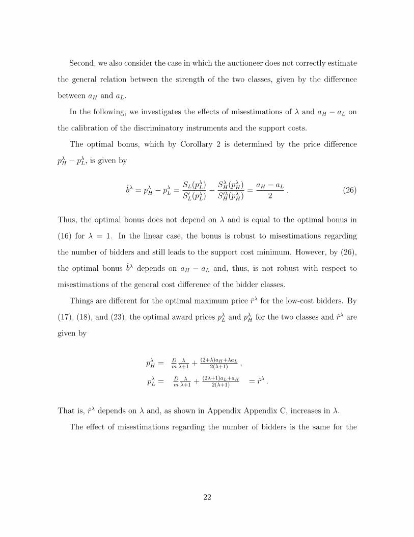
The optimal bonus, which by Corollary 2 is determined by the price difference

pλH − pλL, is given by

bλ = pλH − pλL =SL(pλL)

S ′L(pλL)− SλH(pλH)

S ′λH (pλH)=aH − aL

2. (26)

Thus, the optimal bonus does not depend on λ and is equal to the optimal bonus in

(16) for λ = 1. In the linear case, the bonus is robust to misestimations regarding

the number of bidders and still leads to the support cost minimum. However, by (26),

the optimal bonus bλ depends on aH − aL and, thus, is not robust with respect to

misestimations of the general cost difference of the bidder classes.

Things are different for the optimal maximum price rλ for the low-cost bidders. By

(17), (18), and (23), the optimal award prices pλL and pλH for the two classes and rλ are

given by

pλH = Dm

λλ+1

+ (2+λ)aH+λaL2(λ+1)

,

pλL = Dm

λλ+1

+ (2λ+1)aL+aH2(λ+1)

= rλ .

That is, rλ depends on λ and, as shown in Appendix Appendix C, increases in λ.

The effect of misestimations regarding the number of bidders is the same for the

22

optimal quota Qλ, which with (19), (20), and (23) is determined by

SλH(pλH) = Dλ+1− m

2(λ+1)(aH − aL) = Qλ , (27)

SL(pλL) = Dλλ+1

+ m2(λ+1)

(aH − aL) = D − Qλ .

The optimal quota Qλ depends on λ and, as shown in Appendix Appendix C, decreases

in λ.

Hence, the implementation of the maximum price r yields the same result as the

implementation of Q. That is, a misestimation regarding λ has the same effect if either

a quota or a maximum price is implemented.

Misestimations of the difference aH − aL have the same effect for the optimal maxi-

mum price rλ and the optimal quota Qλ. The volume shift induced by both instruments

qλ =m

2(λ+ 1)(aH − aL) ,

which is given by the difference between (27) and (25) and which depends on λ and

aH−aL. Hence, maximum price and quota are also not robust regarding misestimations

of the general relation between the strength of the bidder classes.

If the auctioneer implements the quota Q, which in this case is equivalent to the

implementation of the maximum price r, the support costs depend on the misestimation

of λ. To see this, consider Kλ(Q), i.e., the support costs depending on a quota Q:

Kλ(Q) = (D − Q) ·MCL(D − Q) + Q ·MCλH(Q) ≥ Kλ(Qλ) . (28)

The equality only holds for λ = 1. If λ 6= 1, the costs Kλ(Q) of the non-optimal quota

Q are higher than the costs Kλ(Qλ) of the optimal quota Qλ and, as shown in Appendix

Appendix C, the difference Kλ(Q)−Kλ(Qλ) increases in |λ− 1|.

23

For λ < 1, Kλ(Qλ) ≤ Kλ(Q) ≤ Kλ(0). That is, discrimination through Q or r still

leads to lower costs than in the free competition case with Q = 0 although the auction-

eer wrongly estimates the relation of the bidder classes (see Appendix Appendix C).

This does not hold for λ > 1. In this case, Kλ(Q) > Kλ(0) is possible, i.e., the imple-

mentation of a non-optimal quota or maximum price leads to higher costs than in the

free competition case without discrimination.

As shown before, the bonus b is (more) robust to wrong estimation of λ. In the

linear model, the optimal bonus does not depend on λ but only on aH −aL. The key to

design a discriminatory auction robust to misestimations of λ is to achieve the optimal

cost difference (26) which is always fulfilled through the optimal bonus.

Q D − Q

r

pλ

H

pH

pλH

Price

Quantity

MCH

MCL

MCλ

H

MCλ

H

Figure 3: Illustration of the extended example with a quota Q and λ < 1 < λ.

Figure 3 illustrates the effect of either the implementation of Q or r on the basis of

different misestimations of λ. The optimal price difference pH − r is only implemented

if the relation of the number of high-cost bidders and low-cost bidders is estimated

correctly. For λ < 1 the price difference is lower than pH − r and, thus, there is

24

potential for further cost reductions. For λ > 1 it is possible that the costs are even

higher than in the free competition case.

4. Conclusion

It is a general trend in the expanded implementation of auctions for RE support to

open the auctions to either multiple technologies or to bidders from several countries.

The corresponding buzzwords are “technology-neutral” and “cross-border” auctions.

As a consequence, designing the auction becomes more complex and more stakeholders

express their opinion and try to shift the design parameters in their favor. Obviously,

the argumentation that more competition always reduces prices falls short. The most

discussed topics regarding more open auction formats for RE support are dynamic

efficiency, integration costs and windfall profits.

We contribute to this discussion by transferring general microeconomic principles

to the RE auction applications. We showed how three different discriminatory auction

design elements – a quota, a bonus and a maximum price – can be implemented in

auctions for RE support and what their implications are. We proved for each instrument

that the discrimination of the stronger bidders in favor of the weaker bidders reduces the

overall support costs. Moreover, to formulate it the other way round, if the introduction

of a discriminatory instrument does not reduce the support costs, then there is no sense

in conducting a non-discriminatory, multi-technology auction because only the strong

technology would be awarded.

Additionally, we proved that the support cost minimum can be achieved by each

of the three instruments if implemented in the optimal way. However, the optimal

implementation of a quota, a bonus, or a maximum price requires information regarding

the cost distribution of the different bidder groups. Depending on the availability of

this information the three instruments vary regarding their robustness.

25

That is, if the auctioneer aims to minimize the support costs, the auction design

should include discriminatory elements. Note, however, that this cost reduction is

at the expense of efficiency. While the effective discrimination reduces the overall

support costs, the awarded bidders are not necessarily those with the lowest generation

costs. This conflict between support cost minimization and efficiency highlights the

importance for the auctioneer to be aware of his targets and their priority.

There is no panacea for designing the “right” auction for the promotion of RE

sources. The design has to be adapted to the target and the current market and

technological developments, possibly including discriminatory instruments.

Appendix A. Proof of Lemma 1

Proof. Let ∆(q) denote the change in the support costs induced by q compared to free

competition, which by (6) and (7) is

∆(q) = MCL(SL(p∗)− q) · (SL(p∗)− q) +MCH(SH(p∗) + q) · (SH(p∗) + q)−K(p∗) .

Differentiating ∆(q) with respect to q, denoted by ∆′(q), yields

∆′(q) = −MC ′L(SL(p∗)− q)(SL(p∗)− q)−MCL(SL(p∗)− q)

+MC ′H(SH(p∗) + q)(SH(p∗) + q) +MCH(SH(p∗) + q) .

Starting with an ineffective quota, q = 0, to prove that the costs decrease when the

quota becomes effective, we have to show that

∆′(0) = −MCL(SL(p∗))−SL(p∗)MC ′L(SL(p∗))+MCH(SH(p∗))+SH(p∗)MC ′H(SH(p∗)) < 0 ,

26

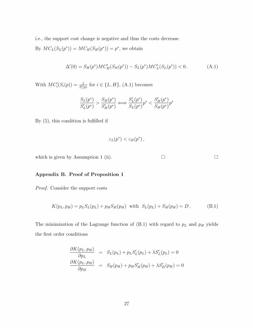
i.e., the support cost change is negative and thus the costs decrease.

By MCL(SL(p∗)) = MCH(SH(p∗)) = p∗, we obtain

∆′(0) = SH(p∗)MC ′H(SH(p∗))− SL(p∗)MC ′L(SL(p∗)) < 0 . (A.1)

With MC ′i(Si(p)) = 1S′i(p)

for i ∈ {L,H}, (A.1) becomes

SL(p∗)

S ′L(p∗)>SH(p∗)

S ′H(p∗)⇐⇒ S ′L(p∗)

SL(p∗)p∗ <

S ′H(p∗)

SH(p∗)p∗

By (5), this condition is fulfilled if

εL(p∗) < εH(p∗) ,

which is given by Assumption 1 (ii).

Appendix B. Proof of Proposition 1

Proof. Consider the support costs

K(pL, pH) = pLSL(pL) + pHSH(pH) with SL(pL) + SH(pH) = D . (B.1)

The minimization of the Lagrange function of (B.1) with regard to pL and pH yields

the first order conditions

∂K(pL, pH)

∂pL= SL(pL) + pLS

′L(pL) + λS ′L(pL) = 0

∂K(pL, pH)

∂pH= SH(pH) + pHS

′H(pH) + λS ′H(pH) = 0

27

which lead to the condition

pH − pL =SL(pL)

S ′L(pL)− SH(pH)

S ′H(pH). (B.2)

For Q ≤ SH(p∗), pH = pL = p∗ and, thus, the left-hand side of (B.2) is zero. Q > SH(p∗)

implies pH > p∗ > pL. With an increasing Q, pH increases and pL decreases and, thus,

the left-hand side of (B.2) increases. (5) and Assumption 1 (ii)imply that the right-

hand side of (B.2) is positive at p∗ which demonstrates that the optimality condition

(B.2) does not hold for an ineffective quota, e.g. Q ≤ SH(p∗. By Assumption 1 (i),

εH(pH) does not increase and εL(pL) does not decrease if pH increases and pL decreases.

Thus, with (5), the right-hand side of (B.2) decreases. Since the left-hand side of (B.2)

increases with an increasing quota Q and the right-hand side of (B.2) decreases, there

exist a unique Q that fulfills (B.2). Together with Lemma 1, that an increasing quota

Q above SH(p∗) reduces the support costs, Q is the unique cost minimum.

Appendix C. Additional Calculations for the Extended Example in Section

3.3

To show that the equilibrium price pλ increases if there are less high-cost bidders

than expected, i.e., λ > 1, we calculate

pλ − p∗ =λ− 1

(λ+ 1)2

(D

m+ aL + aH

)

where (Dm

+ aL + aH) > 0 due to (13) and λ−1(λ+1)2

is greater than zero for λ > 1 and

negative for λ < 1. Therefore, the equilibrium price increases for an increasing λ.

As a direct result, also the support costs Kλ(pλ) are greater than K(p∗) if there are

less high-costs bidders and vice versa with more high-cost bidders.

To prove that the implementation of a quota Q in a case where λ 6= 0 is not optimal,

28

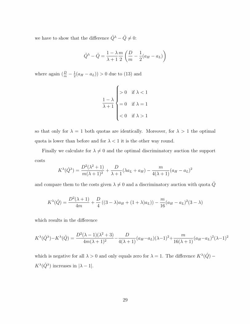
we have to show that the difference Qλ − Q 6= 0:

Qλ − Q =1− λλ+ 1

m

2

(D

m− 1

2(aH − aL)

)

where again (Dm− 1

2(aH − aL)) > 0 due to (13) and

1− λλ+ 1

> 0 if λ < 1

= 0 if λ = 1

< 0 if λ > 1

so that only for λ = 1 both quotas are identically. Moreover, for λ > 1 the optimal

quota is lower than before and for λ < 1 it is the other way round.

Finally we calculate for λ 6= 0 and the optimal discriminatory auction the support

costs

Kλ(Qλ) =D2(λ2 + 1)

m(λ+ 1)2+

D

λ+ 1(λaL + aH)− m

4(λ+ 1)(aH − aL)2

and compare them to the costs given λ 6= 0 and a discriminatory auction with quota Q

Kλ(Q) =D2(λ+ 1)

4m+D

4((3− λ)aH + (1 + λ)aL))− m

16(aH − aL)2(3− λ)

which results in the difference

Kλ(Qλ)−Kλ(Q) =D2(λ− 1)(λ2 + 3)

4m(λ+ 1)2− D

4(λ+ 1)(aH−aL)(λ−1)2+

m

16(λ+ 1)(aH−aL)2(λ−1)2

which is negative for all λ > 0 and only equals zero for λ = 1. The difference Kλ(Q)−

Kλ(Qλ) increases in |λ− 1|.

29

References

Brown A, Beiter P, Heimiller D, Davidson C, Denholm P, Melius J, Lopez A, Hettinger

D, Mulcahy D, Porro G (2016) Estimating Renewable Energy Economic Potential

in the United States: Methodology and Initial Results. Tech. Rep. NREL/TP-6A20-

64503, National Renewable Energy Laboratory (NREL), URL http://www.nrel.

gov/docs/fy15osti/64503.pdf, Accessed: 23.11.2017

Bulow J, Roberts J (1989) The Simple Economics of Optimal Auctions. Journal of

Political Economy 97(5):1060–1090

Bundesnetzagentur (2017a) Ergebnisse der EEG Ausschreibung fur Solaran-

lagen vom 01. Juni 2017. Tech. rep., Bundesnetzagentur fur Elektrizitat,

Gas, Telekommunikation, Post und Eisenbahnen, URL https://www.

bundesnetzagentur.de/SharedDocs/Downloads/DE/Sachgebiete/Energie/

Unternehmen_Institutionen/Ausschreibungen_2017/Hintergrundpapiere/

Hintergrundpapier_01_06_2017.pdf?__blob=publicationFile&v=6, Accessed:

23.11.2017

Bundesnetzagentur (2017b) Ergebnisse der EEG Ausschreibung fur Windenergiean-

lagen an Land vom 01. Mai 2017. Tech. rep., Bundesnetzagentur fur Elek-

trizitat, Gas, Telekommunikation, Post und Eisenbahnen, URL https://www.

bundesnetzagentur.de/SharedDocs/Downloads/DE/Sachgebiete/Energie/

Unternehmen_Institutionen/Ausschreibungen_2017/Hintergrundpapiere/

Hintergrundpapier_OnShore_01_05_2017.pdf?__blob=publicationFile&v=2,

Accessed: 23.11.2017

Centro Nacional de Control de Energia (2017) Bases de Licitacion de la Sub-

asta de Largo Plazo SLP-1/2017. URL http://www.cenace.gob.mx/Docs/

30

MercadoOperacion/Subastas/2017/07%20Bases%20Licitacion%20SLP2017%

20v08%2005%202017.zip, Accessed: 19.01.2018

Department for Business, Energy & Industrial Strategy (2017) FiT Contract for Dif-

ference Standard Terms and Conditions. URL https://www.gov.uk/government/

uploads/system/uploads/attachment_data/file/590368/FINAL_draft_CFD_

-_Standard_Conditions_-_Amendments_Feb_2017_-_tracked.pdf, Accessed:

25.01.2018

Department of Energy and Climate Change (2011) Planning our electric fu-

ture: a White Paper for secure, affordable and low-carbon electricity.

White paper, URL https://www.gov.uk/government/uploads/system/uploads/

attachment_data/file/48129/2176-emr-white-paper.pdf, Accessed: 18.01.2018

Deutscher Bundestag (2016) Gesetz zur Einfuhrung von Ausschreibungen fur Strom

aus erneuerbaren Energien und zu weiteren anderungen des Rechts der erneuerbaren

Energien. URL https://dipbt.bundestag.de/dip21/brd/2016/0355-16.pdf, Ac-

cessed: 23.11.2017

European Commission (2014) Guidelines on State aid for environmental protec-

tion and energy 2014-2020 (2014/C 200/01). URL http://eur-lex.europa.eu/

legal-content/EN/TXT/?uri=CELEX:52014XC0628(01), Accessed: 23.11.2017

Held A, Ragwitz M, Haas R (2006) On the Success of Policy Strategies for the Promo-

tion of Electricity from Renewable Energy Sources in the EU. Energy & Environment

17(6):849–868, DOI 10.1260/095830506779398849

Hoefnagels R, Junginger M, Panzer C, Resch G, Held A (2011)

Long Term Potentials and Costs of RES. D10 report, RE-

31

Shaping, URL http://www.reshaping-res-policy.eu/downloads/D10_

Long-term-potentials-and-cost-of-RES.pdf, Accessed: 23.11.2017

IRENA (2015) Renewable Power Generation Costs in 2014. Tech. rep., International

Renewable Energy Agency, URL https://www.irena.org/DocumentDownloads/

Publications/IRENA_RE_Power_Costs_2014_report.pdf, Accessed: 23.11.2017

IRENA (2017) Renewable Energy Auctions: Analysing 2016. Tech. rep., International

Renewable Energy Agency, URL http://www.irena.org/DocumentDownloads/

Publications/IRENA_Renewable_Energy_Auctions_2017.pdf, Accessed:

23.11.2017

Joskow PL (2011) Comparing the costs of intermittent and dispatchable electricity

generating technologies. The American Economic Review 101(3):238–241

Kitzing L, Wendring P (2016) Cross-border auctions for solar PV -

the first of a kind. URL http://auresproject.eu/publications/

cross-border-auctions-solar-pv-the-first-of-a-kind, Accessed: 22.01.2018

Kreiss J, Ehrhart KM, Haufe MC, Soysal ER (2017) Different cost perspectives

for renewable energy support: Assessment of technology-neutral and discrim-

inatory auctions. Forthcomming URL http://games.econ.kit.edu/downloads/

TNandDiscriminatoryREAuctions__KrEhHaSR.pdf, Accessed: 22.01.2018

McAfee R, McMillan J (1989) Government procurement and international trade. Jour-

nal of International Economics 26(3):291 – 308, DOI 10.1016/0022-1996(89)90005-6

Minister van Economische Zaken (2015) Besluit stimulering duurzame energieproduc-

tie. URL http://wetten.overheid.nl/jci1.3:c:BWBR0022735&z=2015-05-30&g=

2015-05-30, Accessed: 25.01.2018

32

Ministerio de Energia, Turismo y Agenda Digital (2017a) Real Decreto 359/2017. Bo-

letin Oficial del Estado, Num. 78, Sec. III. Pag. 25504, URL https://www.boe.es/

buscar/doc.php?id=BOE-A-2017-3639, Accessed: 23.01.2018

Ministerio de Energia, Turismo y Agenda Digital (2017b) Real Decreto 650/2017. Bo-

letin Oficial del Estado, Num. 144, Sec. III. Pag. 50550, URL http://www.boe.es/

boe/dias/2017/06/17/pdfs/BOE-A-2017-6940.pdf, Accessed: 29.01.2018

Myerson RB (1981) Optimal auction design. Mathematics of Operations Research

6(1):58–73, DOI 10.1287/moor.6.1.58

Public Utilities Commission of the State of California (2010) Decision adopting the Re-

newable Auction Mechanism. URL http://docs.cpuc.ca.gov/word_pdf/FINAL_

DECISION/128432.pdf, Accessed: 23.11.2017

Schmalensee R (1981) Output and Welfare Implications of Monopolistic Third-Degree

Price Discrimination. The American Economic Review 71(1):242–247

Short W, Packey DJ, Holt T (1995) A Manual for the Economic Evaluation of Energy

Efficiency and Renewable Energy Technologies. Tech. rep., National Renewable En-

ergy Laboratory (NREL), URL http://www.nrel.gov/docs/legosti/old/5173.

pdf, Accessed: 23.11.2017

Thiel SE (1988) Multidimensional auctions. Economics Letters 28(1):37 – 40, DOI

https://doi.org/10.1016/0165-1765(88)90068-7

Ueckerdt F, Hirth L, Luderer G, Edenhofer O (2013) System LCOE: What are the costs

of variable renewables? Energy 63:61 – 75, DOI 10.1016/j.energy.2013.10.072

Varian HR (1989) Chapter 10 Price discrimination. In: Handbook of Industrial Orga-

nization, vol 1, Elsevier, pp 597 – 654, DOI 10.1016/S1573-448X(89)01013-7

33

de Vries BJ, van Vuuren DP, Hoogwijk MM (2007) Renewable energy sources: Their

global potential for the first-half of the 21st century at a global level: An integrated

approach. Energy Policy 35(4):2590 – 2610, DOI 10.1016/j.enpol.2006.09.002

Weber RJ (1983) Multiple-Object Auctions. In: Shubik M, Stark RM, Engelbrecht-

Wiggans R (eds) Auctions, Bidding, and Contracting: Uses and Theory, New York

University Press, chap Issues in Theory of Auctions, pp 165–191

Wigand F, Forster S, Amazo A, Tiedemann S (2016) Auctions for Renewable Energy

Support: Lessons Learnt from International Experiences. Reseaarch report, AU-

RES, URL http://auresproject.eu/sites/aures.eu/files/media/documents/

aures_wp4_synthesis_report.pdf, accessed: 23.11.2017

34