NPAFC

Doc. No.2lL

Rev. No.

Discrimination Of Thermally-Marked Otoliths From Unmarked Specimens By Machine Learning Of Texture Characteristics

By

S. Hickinbothaml, P. Hagen2

, E.Hancock1, and J. Austinl

1 University of York, Heslington, York UK YOl 5DD.

2 Alaska Department ofFish and Game, P.O. Box 25526 Juneau, Alaska 99821-5526

Submitted to the NORTH PACIFIC ANADROMOUS FISH COMMISSION

by the UNITED ST ATES PARTY

October 1998

This paper may be cited in the following manner: Hikinbotharn, S., P. Hagen, E. Hancock, J. Austin. 1998. Discrimination of thermally-marked otoliths from unmarked specimens by machine learning of texture characteristics. (NPAFC Doc. 371). 13p. Alaska Dept. Fish and Game, Juneau Alaska. 99801-5526

Discrimination of thermally-marked otoliths from unmarked specimens by machine learning of texture characteristics

Simon J. Hickinbotham1, Peter Hagen2 , Edwin R. Hancockl and James Austin l

1: University of York, Heslington, York YOl 5DD, UK. sjh@minster.york.ac.uk

2: Alaska Department of Fish and Game, Juneau, Alaska 99802-5526, USA.

Abstract

\Ve adopt a novel approach to detecting thermal marks using techniques that are being developed for texture discrimination in computer vision. This provides a more natural framework for thermal mark detection than the line detector schemes that are commonly proposed because the detection and inter-mark distance measurement are combined in a single filtering step. We decompose the image into a multi-channel representation using a bank of Gabor filters that has been previously tuned to discriminate thermal marks. We learn the pattern of filter responses by using the Expectation - Maximisation algorithm of Dempster, Laird and Rubin to fit a mixture Gaussian model to the data. We arrive at a hard classification of the data by assigning different components of the model to foreground or background classes. The approach is evaluated by examining test samples containing a mixture of known otoliths from thermally marked hatchery and wild pink salmon fry from Prince William Sound, Alaska. The advantages and disadvantages of computer vision in this application are considered.

1. INTRODUCTION

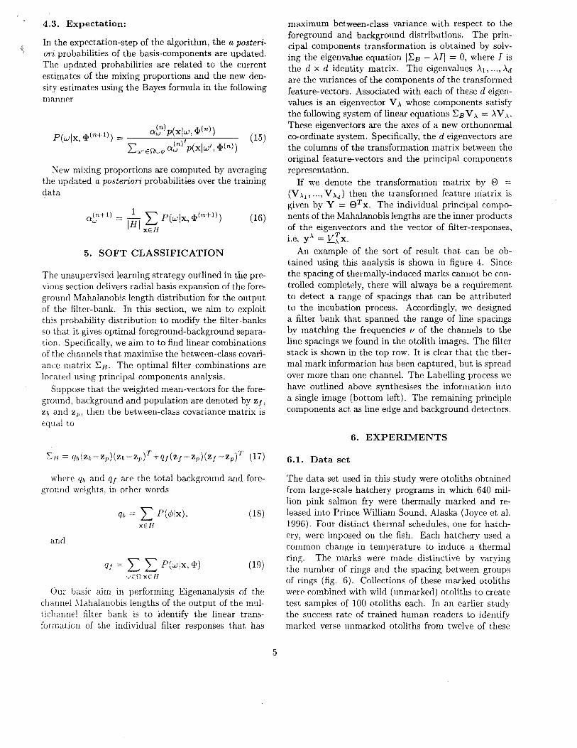
Thermal marking of otoliths is a method by which tem­perature manipulations during early growth are used to induce a set of patterns into the otolith microstructure of hatchery fish (Volk et al., 1990). These patterns (see figure 1) can be recovered in otoliths of adult salmon captured in commercial fisheries and the information is being used to help manage mix-stock fisheries (Ha­gen et al.. 1995). Readers identify thermal marks by examining example patterns in otoliths from a sample of marked fish collected prior to release and then look for those patterns in otoliths of the adults of unknown origin, A good thermal mark contains contrast and fre­quency characteristics that allow it to stand out from background patterns and 'noise' in wild stocks otoliths.

As with many such tasks which involve identifying patterns ill biological samples, the human vision sys­tell! ami decision making process is not easily emulated with lIlachine vision approaches (Glaseby and Horgan,

However by examining the pattern characteris­tics that allow a thermal marks to be recognised as dis­tinnin'. we can recognise opportunities to help semi­autolllate the process and help improve the ability to make thermal patterns. This paper presents the first

1

step towards applying advanced image analysis meth­ods to the task of identifying thermal marks using tech­niques developed for texture analysis in the computer vision research community.

The texture of an image is not an easy characteris­tic to measure or to define (Pratt, 1991). In essence texture analysis attempts to quantify repetitive struc­tures within two-dimensional arrays of variation. A relatively new approach to examine otoliths and other biological structures that grow by accretion, is to pro­cess the image through a bank of Gabor filters (Hick­inbotham et al., 1996). This is often referred to as the multi-channel filtering approach. The basic idea is to represent quite intricate grey-scale appearance using the response pattern of a high-dimensional filter bank. These filter banks are designed so that the channels are distributed over representative scales, orientations and feature symmetries. In this application domain, Gabor filters are the obvious choice, since they can be tuned to respond to line textures of particular spacing. The image can be decomposed into a set of sub-images, each of which can be tuned to respond to different fea­hIres in the image (Jain and Farrokhnia, 1991). The task then is to examine the channel responses to obtain a meaningful classification of the pixels in the original

image. For our purposes, the filters can be tuned to re­spond to spacings of lines that match those formed in the thermal marking process. In this context, we can think of otolith images as examples of line textures, i.e. a texture in which the dominant pattern is formed by approximately concentric lines.

The aims of this paper are to introduce texture anal­ysis methodologies to the application domain of detec­tion of thermally-marked otoliths, and to give a de­tailed example of the experiments we have carried out to develop a more dedicated application. The first of these aims will be met by an introduction to Gabor filter banks, methods of tuning filters to respond to target textures and examination of the pixel-labelling process. The second aim of this paper will be met ,by describing a statistical methodology for learning combinations of channel filters for feature characterisa­tion. The learning procedure is non-linear and is based on the Expectation-Maximisation (EM) algorithm of Dempster, Laird and Rubin (Dempster et al., 1977). The EM algorithm uses Bayesian probability theory to fit a model to data by iteratively recalculating the parameters of the model's components and their prior probabilities.

We commence from a similar starting point to that of Bregler and Malik (Bregler and Malik, 1996), by adopting the EM algorithm as a learning engine. How­ever, our methodology differs in a number of important respects.

In the first instance we commence by performing channel balancing so as to ensure that each of the com­ponents of the filter bank has an equal noise through­put. This is effected by computing the variance­covariance matrix for the filter kernels. The ele­ments of the matrix are the auto-correlations and cross­correlations of the individual kernels in the filter-bank. 'Cnder the assumption that the image is subjected tq additiye Gaussian noise of zero mean, the noise­response of the filter bank follows a multivariate normal distribution which is characterised by the Mahalanobis length of the integrated channel-vector. This channel noise model provides a background probability distri­bution.

In order to model the unknown foreground feature distribution for the channel responses, we adopt a radial-basis distribution. The basic idea is to fit a se­ries of Gaussian basis functions to the residue of the probability distribution when the background process is subtracted. The parameterised distribution is used to compute a posteriori feature probabilities in the ex­pectation step of the learning process.

Finally, once the a posteriori feature probabilities are to hand they' may be used to project out the optimal

2

set of channel combinations for the foreground or target features. Here we use the between class covariance ma­trix as a foreground-background separation measure. We project out linear filter combinations by applying principal components analysis to the between class co­variance matrix.

The outline of this paper is as follows. Section 2 discusses how to use Gabor filter banks as line texture discriminators. Section 3 reviews methods of synthe­sising multichannel feature representations into mean­ingful segmentations. An experimental eyaluation of a method to detect thermally marked otoliths is de­scribed in section 4, and results are presented and dis­cussed in section 5. Concluding remarks can be found in section 6.

2. THE MULTICHANNEL GABOR FILTER BANK

Although it wasn't realized at the time, the first indi­cation that Gabor filters could be used in vision came with the work of Hubel and Wiesel in 1962 (Hubel and Wiesel, 1962). They described the neural inputs to cells of the visual cortex that were arranged in elon­gated areas of excitation and inhibition. Although they suggested that this was a localised tuning of cells to specific frequencies in the image, the connection with the Gabor function was not realised for nearly twenty years. The connection was finally made simultaneously by Daugman (Daugman, 1980) and Marcelja (Marcelja, 1980), which sparked a surge of interest in the use of Gabor filters in machine vision that has continued to this day.

We can develop a model of an image in which the 2D signal is represented in terms of the magnitude, phase and orientation of a set of sinusoids in that image. The whole image can be represented in terms of these sinusoids by it's Fast Fourier Transform (FFT). The basis of using Gabor functions as filters is that they can be used to pick out locally dominant sinusoids in the image. The problem then is selecting a combination of sinusoids that are capable of discriminating the target texture from other image features

Gabor filters are calculated by taking the product of a Gaussian window and a complex sinusoid. The Gaussian window controls the region of influence that the filtering process uses in calculating it's response. The frequency and orientation of the sinusoid is tuned to match the features that are to be discriminated.

If i and j denote the spatial co-ordinates, then Ga­bor functions with horizontal orientation having spatial width (Ji and (Jj, and frequency v are as follows

C",tT.o(i,j) = exp -- ;. + ; cos [21!'vi] [

1 ( '2 '2)] 2 a i aj

(1)

[ 1 ( '2 '2)] S",tT,o(i,j)=exp -2 :t+~] sin [21!'vi] (2)

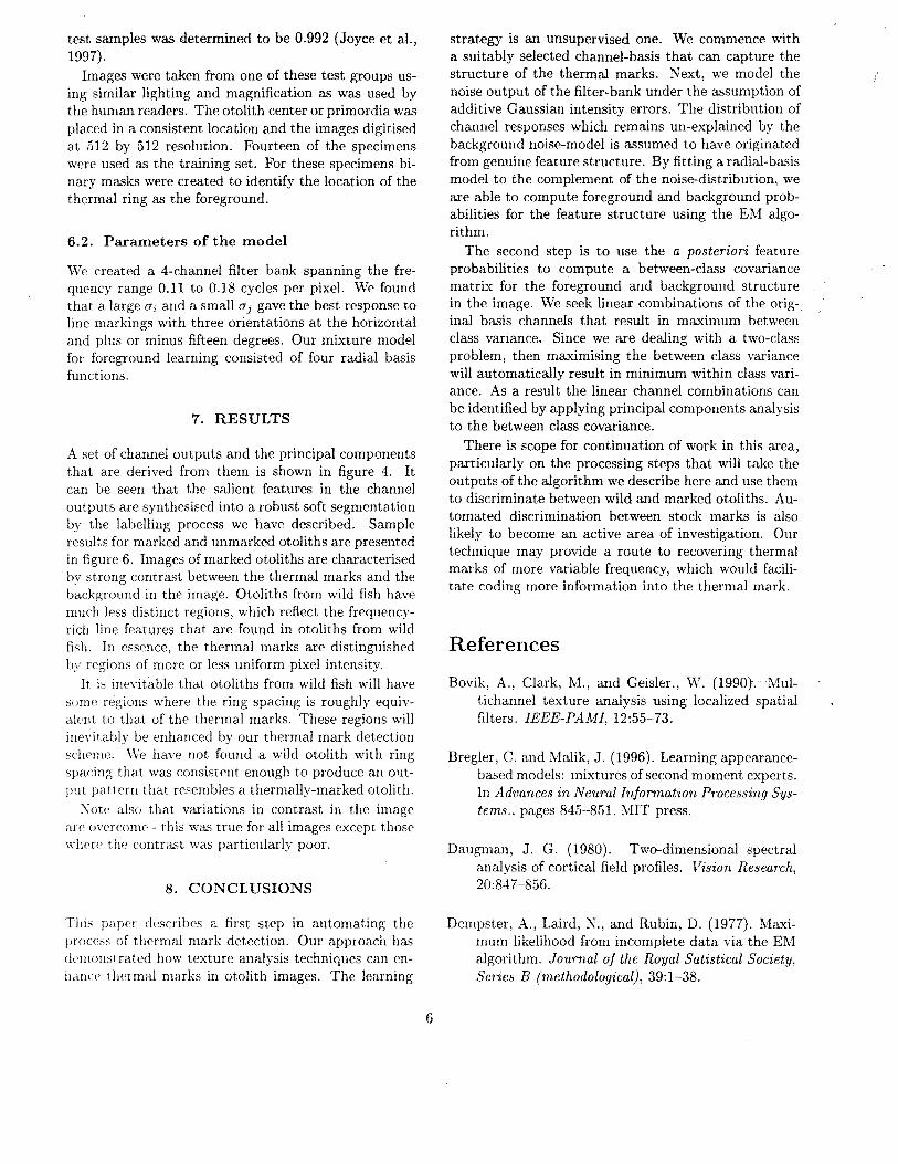
Since it is of even symmetry, the cosine-phase Ga­bor kernel C",tT,o(i, j) operates as a line-enhancement operator. The sine-phase kernel, on the other hand, is appropriate to edge-detection. In this application, a is fixed and three orientations () are used. For the sake of shorthand convenience, we write the image and fil­ter pixel lattices as A, C",1i and S",o respectively. An image F is filtered by Fourier convolution (denoted by the symbol 0) with C",II and S",o. In order to obtain a uniform response to a line texture pattern, the "texture energy" of the filter pair is calculated as

J 2 2 EII,II = (A 0 CII,o) + (A 0 S",o) (3)

Since we intend to recognise thermal marks regard­less of orientation, we take the modulus of the oriented Texture energy responses to form a single channel W ,,:

15°

L E~o (4) 11=-15°

This filter-bank is composed of filters of a range of frequencies to form the image vector

x=

where d is the number of channels in the filter bank. From here on we refer to an individual pixel vector as x. since calculations will be carried out on all pixels indexed i, j ill the chanllel stack X.

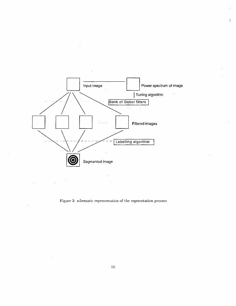
The overall aim of texture analysis in computer vi­SiOll is to segregate an image into meaningful regions of separate textures. This is achieved by what is known a" a labelling process. whereby every pixel in an image is a:;sil!;llt'd a value that indicates which of a number of

in t Itt' image the pixel belongs to. The process i~ illustrated in figure 3. There are three major stages to all\' texture st'gmentation algorithm. The first stage is the s('l('ction and tuning of the filters that are to be applied to the image. This has often been a very ad hoc affair. bur. recent work (Tan, 1995; Bovik et aI.,

3

1990) has demonstrated methods of identifying candi­date filter banks by examination of the Fourier power spectrum of the image under consideration. Automa­tion of this process by fuzzy clustering (Hickinbotham et aI., 1996) has enabled tuning of filters to be car­ried out unsupervised. However, since thermal marks produce features of more or less constant spacing, the range of pertinent frequencies in the otolith images can be easily determined empirically by manual examina­tion of the Fourier power spectra of a subset of the images.

The resulting multichannel representation of the fea­tures in the image is an expansion of each pixel in the image into a vector of values corresponding to strength of a particular feature that particular pixel location. In this example, we arrive at a channel stack that contains information about the dominant frequencies at a par­ticular location. These frequencies correspond to the line spacing of the thermal marks on the otoliths. A high response indicates that the presence of a thermal mark at that particular image location is likely. We thus arrive at a much more controllable representation of the features in the image.

3. CHANNEL COMBINATION

The final process is to resolve the pixel vectors into a label for each pixel. This is the most difficult part of the process and has given rise to a wide range of methodologies.

One of the key issues that raises itself when a multi­channel feature or object representation is used is that of how to learn the pattern of filter responses. The literature here is relatively sparse. Most of the work which exploits neural network architectures adopts the working model that the recognition process should be trained from a few examples and that the generalisation properties of the network should be exploited to accom­modate variable object appearance (Rao and Ballard, 1997). An example of a more principled approach is Bregler and Maliks (Bregler and Malik, 1996) use of the expectation-maximisation (Dempster et al. , 1977) al­gorithm to learn the channel mixing proportions. This procedure has been demonstrated to work effectively on relatively noise-free and uncluttered imagery.

3.1. Background

Our statistical modelling of the filter-bank output com­mences by considering the image background class ¢. Here we assume that the filters are being applied to locally uniform image regions containing no significant features or structure. We further assume that the uni­form structure less regions are subject to additive Gaus-

sian noise with zero mean. Since the filter responses are obtained in a linear fashion from the noisy image data, then the channel response vector x follows a mul­tivariate Gaussian with zero mean. In other words, the probability density function for the background distri­bution of channel-vectors is the distribution

( I ) 1 1 [1 T -1 ] P X ¢ = ~ exp - -x I:q, X (27r) V 1I:q,1 2

(6)

Where I:q, is the covariance matrix of the channel­vectors, equivalent to the expectation value of XXT

and xT I:;lx is the Mahalanobis length of x. This noise distribution will be used to model the background con­tributions in our training data.

3.2. Foreground

The statistical modelling of the foreground distribu­tion of Mahalanobis length for feature detection has proved to be an extremely elusive task. For instance, attempts at modelling the distribution of edge-gradient for automatic control of the Canny hysteresis thresh­olds have confined their attention to the background or noise process (Voorhees and Poggio, 1987; Hancock and Kittler, 1990) . In this paper our aim is to use the background model to assist in learning the channel structure of the foreground. Specifically, we augment the Gaussian background model with a radial basis ex­pansion to which we use to parameterise foreground structure. We distinguish between the different basis kernels by assigning them a label w . The complete set of foreground kernels is denoted by the set n. The kernel indexed w has mean Mahalanobis length flw and mixing proportion Q w . The basis functions are as­sumed to have a radial structure. In other words, the channel covariance matrix is diagonal with identical el­ements and is of the .form I:w = a~I where I is the . identity matrix. With these ingredients the basis ker­nel indexed w is

1 exp[-~(X-fl fI:-1(x-fl)] aw 2 ---.: w -w

(7) when' <1>..; represents the set of basis parameters for

t he kernel indexed w:

(8)

Finally. the radial-basis approximation of the fore­ground is

p(xln) = L Q..;p(xlw, <1» (9) wEll

4

The complete model of the filter outputs can then be expressed as follows

p(x) = Qq,p(xl¢) + L Qwp(xlw, <1» (10) wEll

4. LEARNING

In this section we outline our learning algorithm. This is based on the EM algorithm. The idea is to iterate be­tween expectation and maximisation steps to learn the parameters of the foreground radial-basis expansion.

4.1. Objective Measure:

Stated succinctly, we use the foreground radial basis expansion to model the distribution of channel-vectors which remains unexplained by the background process. In order to capture this process in a statistical frame­work we measure the Kullback divergence between the component basis kernels and the complement of the background distribution. The quantity of interest is

K(<I>(nH)I<I>(n») = L L P(wlx, <I>(n») In p~(--,xl_<I>-;-(n-,-H.,..:-») xEH wEll 1 - p(xl¢)

(ll) where H is the set of Mahalanobis lengths of each

data point making up the image. The basic aim is minimise K( <I>(n+l) 1<I>(n») with respect to the mixing proportions, mean channel-vectors and radial covari­ance parameters for the set of basis functions. The solution to this problem is well-known and is furnished by the EM algorithm (Jordan and Jacob, 1994).

4.2. Maximisation:

In the maximisation step we aim to recover maximum likelihood basis-parameters which satisfy the condition

<I>(nH) = argmax K(<I>I<I>(n») (12) q.

At iteration n of the algorithm, the position of the basis-function indexed w is given by

(nH) _ LXEH(l - P(xl¢))P(wlx, <I>(n») flw - LXEH P(wlx, <I>(n»)

(13)

The corresponding basis-function width is equal to

4.3. Expectation:

In the expectation-step of the algorithm, the a posteri­ori probabilities of the basis-components are updated. The updated probabilities are related to the current estimates of the mixing proportions and the new den­sity estimates using the Bayes formula in the following manner

(n) (I <p(n») P(wlx, <p(nH») = a w p x ~' (15)

Lw'EOU¢ aSn) p(xlwl

, <p(n»)

New mixing proportions are computed by averaging the updated a posteriori probabilities over the training data

aSnH ) = I~I L P(wlx, <p(n+l») (16) xEH

5. SOFT CLASSIFICATION

The unsupervised learning strategy outlined in the pre­vious section delivers radial basis expansion of the fore­ground Mahalanobis length distribution for the output of the filter-bank. In this section, we aim to exploit this probability distribution to modify the filter-banks so that it gives optimal foreground-background separa­tion. Specifically, we aim to to find linear combinations of the channels that maximise the between-class covari­ance matrix :B B. The optimal filter combinations are located using principal components analysis.

Suppose that the weighted mean-vectors for the fore­ground, background and population are denoted by z" Zb and zP' then the between-class covariance matrix is equal to

where qb and q, are the total background and fore­ground weights, in other words

qb = L P(1)lx), (18) xEH

and

q, L L P(wlx, <p) (19) wEn xEH

Our basic aim in performing Eigenanalysis of the channel :\lahalanobis lengths of the output of the mul­tichannel filter bank is to identify the linear trans­formation of the individual filter responses that has

5

maximum between-class variance with respect to the foreground and background distributions. The prin­cipal components transformation is obtained by solv­ing the eigenvalue equation I:BB - All = 0, where I is the d x d identity matrix. The eigenvalues AI, ... , Ad are the variances of the components of the transformed feature-vectors. Associated with each of these d eigen­values is an eigenvector V A whose components satisfy the following system of linear equations :BB V A = AVA. These eigenvectors are the axes of a new orthonormal co-ordinate system. Specifically, the d eigenvectors are the columns of the transformation matrix between the original feature-vectors and the principal components representation.

If we denote the transformation matrix by e = (V AI' ... , V Ad) then the transformed feature matrix is given by Y = eT x. The individual principal compo­nents of the Mahalanobis lengths are the inner products of the eigenvectors and the vector of filter-responses, i.e. yA = vT x.

An example of the sort of result that can be ob­tained using this analysis is shown in figure 4. Since the spacing of thermally-induced marks cannot be con­trolled completely, there will always be a requirement to detect a range of spacings that can be attributed to the incubation process. Accordingly, we designed a filter bank that spanned the range of line spacings by matching the frequencies v of the channels to the line spacings we found in the otolith images. The filter stack is shown in the top row. It is clear that the ther~ mal mark information has been captured, but is spread over more than one channel. The Labelling process we have outlined above synthesises the information into a single image (bottom left). The remaining principle components act as line edge and background detectors.

6. EXPERIMENTS

6.1. Data set

The data set used in this study were otoliths obtained from large-scale hatchery programs in which 640 mil­lion pink salmon fry were thermally marked and re­leased into Prince William Sound, Alaska (Joyce et al. 1996). Four distinct thermal schedules, one for hatch­ery, were imposed on the fish. Each hatchery used a common change in temperature to induce a thermal ring. The marks were made distinctive by varying the number of rings and the spacing between groups of rings (fig. 6). Collections of these marked otoliths were combined with wild (unmarked) otoliths to create test samples of 100 otoliths each. In an earlier study the success rate of trained human readers to identify marked verse unmarked otoliths from twelve of these

test samples was determined to be 0.992 (Joyce et al., 1997).

Images were taken from one of these test groups us­ing similar lighting and magnification as was used by the human readers. The otolith center or primordia was placed in a consistent location and the images digitised at 512 by 512 resolution. Fourteen of the specimens were used as the training set. For these specimens bi­nary masks were created to identify the location of the thermal ring as the foreground.

6.2. Parameters of the model

We created a 4-channel filter bank spanning the fre­quency range 0.11 to 0.18 cycles per pixel. We found that a large ai and a small aj gave the best response to line markings with three orientations at the horizontal and plus or minus fifteen degrees. Our mixture model for foreground learning consisted of four radial basis functions.

7. RESULTS

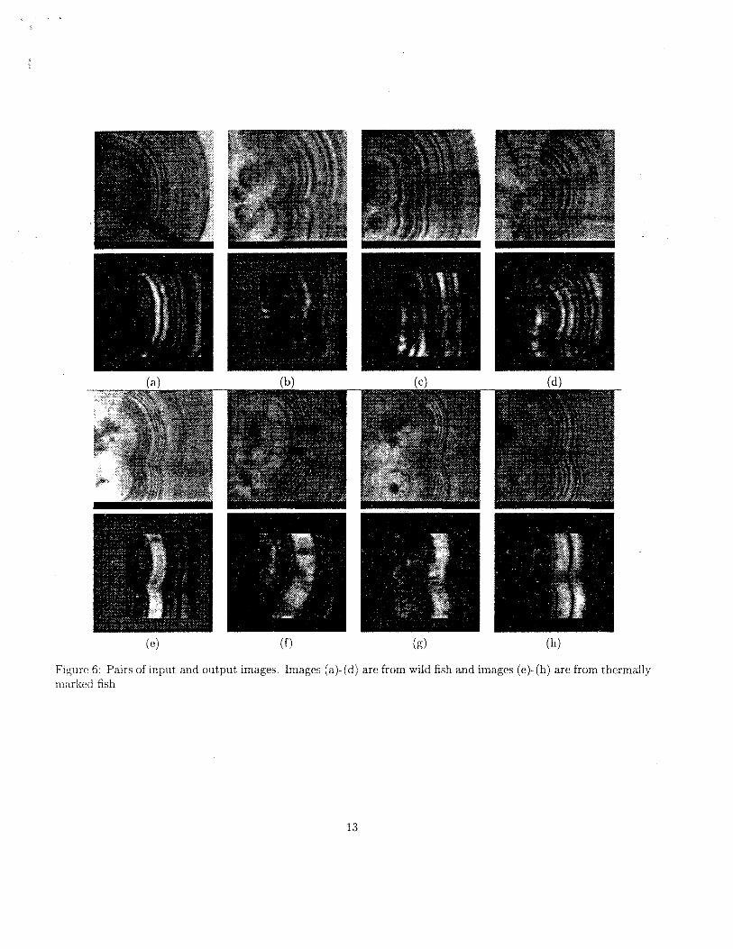
A set of channel outputs and the principal components that are derived from them is shown in figure 4. It can be seen that the salient features in the channel outputs are synthesised into a robust soft segmentation by the labelling process we have described. Sample results for marked and unmarked otoliths are presented in figure 6. Images of marked otoliths are characterised by strong contrast between the thermal marks and the background in the image. Otoliths from wild fish have much less distinct regions, which reflect the frequency­rich line features that are found in otoliths from wild fish. In essence, the thermal marks are distinguished by regions of more or less uniform pixel intensity.

It is ine\'itable that otoliths from wild fish will have SOIJj(' regions where the ring spacing is roughly equiv­alent to that of the thermal marks. These regions will inevitably be enhanced by our thermal mark detection scheme. We have not found a wild otolith with ring spacing that was consistent enough to produce an out­put pattern that resembles a thermally-marked otolith.

:\ote also that variations in contrast in the image are overcome - this was true for all images except those w hert' t he contrast was particularly poor.

8. CONCLUSIONS

This papPI' describes a first step in automating the process of thermal mark detection. Our approach has d('!llOllstrated how texture analysis techniques can en­hanc(' thermal marks in otolith images. The learning

6

strategy is an unsupervised one. We commence with a suitably selected channel-basis that can capture the structure of the thermal marks. Next, we model the noise output of the filter-bank under the assumption of additive Gaussian intensity errors. The distribution of channel responses which remains un-explained by the background noise-model is assumed to have originated from genuine feature structure. By fitting a radial-basis model to the complement of the noise-distribution, we are able to compute foreground and background prob­abilities for the feature structure using the EM algo­rithm.

The second step is to use the a posteriori feature probabilities to compute a between-class covariance matrix for the foreground and background structure in the image. We seek linear combinations of the orig­inal basis channels that result in maximum between class variance. Since we are dealing with a two-class problem, then maximising the between class variance will automatically result in minimum within class vari­ance. As a result the linear channel combinations can be identified by applying principal components analysis to the between class covariance.

There is scope for continuation of work in this area, particularly on the processing steps that will take the outputs of the algorithm we describe here and use them to discriminate between wild and marked otoliths. Au­tomated discrimination between stock marks is also likely to become an active area of investigation. Our technique may provide a route to recovering thermal marks of more variable frequency, which would facili­tate coding more information into the thermal mark.

References

Bovik, A., Clark, M., and Geisler., W. (1990). Mul­tichannel texture analysis using localized spatial filters. IEEE-PAMI, 12:55-73.

Bregler, C. and Malik, J. (1996). Learning appearance­based models: mixtures of second moment experts. In Advances in Neural Information Processing Sys­tems., pages 845--851. MIT press.

Daugman, J. G. (1980). Two-dimensional spectral analysis of cortical field profiles. Vision Research, 20:847-856.

Dempster, A., Laird, N., and Rubin, D. (1977). Maxi­mum likelihood from incomplete data via the EM algorithm. Journal of the Royal Satistical Society, Series B (methodological), 39:1-38.

Glaseby, C. and Horgan, G. (1995). Image analysis for the biological sciences. John Wiley and Sons, New York.

Hagen, P., Munk, K., Alen, B. V., and White, B. (1995). Thermal mark technology for inseason fish­eries management: a case study. Alaska Fishery Research Bulletien, 2(2):143-155.

Hancock, E. and Kittler, J. (1990). edge labelling using dictionary-based relaxation. IEEE PAMI, 12:165-181.

Hickinbotham, S., Hancock, E., and Austin, J. (1996). Segmenting modulated line textures with S-Gabor filters. In Proceedings of the IEEE International Conference on Image Processing, pages 149-152. IEEE.

Hubel, D. and Wiesel, T. (1962). Receptive fields, binocular interaction and functional architecture in the eat's visual cortex. Journal of Physiology, 160:106-154.

Jain, A. and Farrokhnia, F. (1991). Unsupervised tex­ture segmentation using Gabor filters. Pattern Recognition, 24:1167-1186.

Jordan. ~f. 1. and Jacob, R. A. (1994). Hierarchical mixtures of experts and the em algorithm. Neural Computation, 6: 181-.

Joyce. T.) Evans, D., and Munk, K. (1997). Otolith marking of pink salmon in prince william sound hatcheries, 1996, exxon valdez oil spill restora­tion project annual report (restoration project 96188). Technical report, Alaska Department of Fish and Game, Commercial Fisheries Manage­lIlent and Development Division, Cordova, Alaska.

IVIarcelja, S. (1980). Mathematical description of the responses of simple cortical cells. Journal of the Optical Society of America, 70:1297-1300.

Pratt, W. (1991). Digital image processing. John Wiley and Sons, I\ew York, second edition.

Rao, R. P. I\. and Ballard, D. H. (1997). Dynamic model of visual recognition predicts neural re­sponse properties in the visual cortex. Neural Computation. 9:721··763.

Tall. T. (1995). Texture edge detection by mod­elling visual cortical channels. Pattern Recogni­tum. 28:1283-1298.

\'olk. E.) Schroder, S., and Fresh, K. (1990). Induce­lllent of unique otolith banding patterns as a prac­tical means to mass-mark juvenile pacific salmon.

7

In American Fisheries Society Symposium 7, pages 203-215.

Voorhees, H. and Poggio, T. (1987). Detecting textons and texture boundaries in natural images. In Pro­ceedings of the First International Conference on Computer Vision, pages 250-258. Computer Soci­ety Press.

6 U !l U

" [) :} IJ 2 0 1 0 Q 0

SPEEL 1911) BY

~---J-~ Figure 1: Thermal marking of a salmon otolith. The bottom plot shows the temperature fluctuations that induce the ring pattern in the otolith.

8

Figure 2: A cosine Gabor filter, of horizontal orientation. The filter acts as a template for the sort of patterns it i~ tUlled to respond to, regardless of position in the image.

9

D Input image D Power spectrum of image

I Tuning algorithm 7\·- - - -jSank of Gabor filters

DDD D Filtered images

--\-/---- -- -1 Labelling algorithm

I @) I Segmented Image

Figure 3: schematic representation of the segmentation process

10

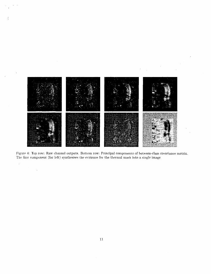
Figure 4: Top row: Raw channel outputs. Bottom row: Principal components of between-class covariance matrix. The first component (far left) synthesises the evidence for the thermal mark into a single image

11

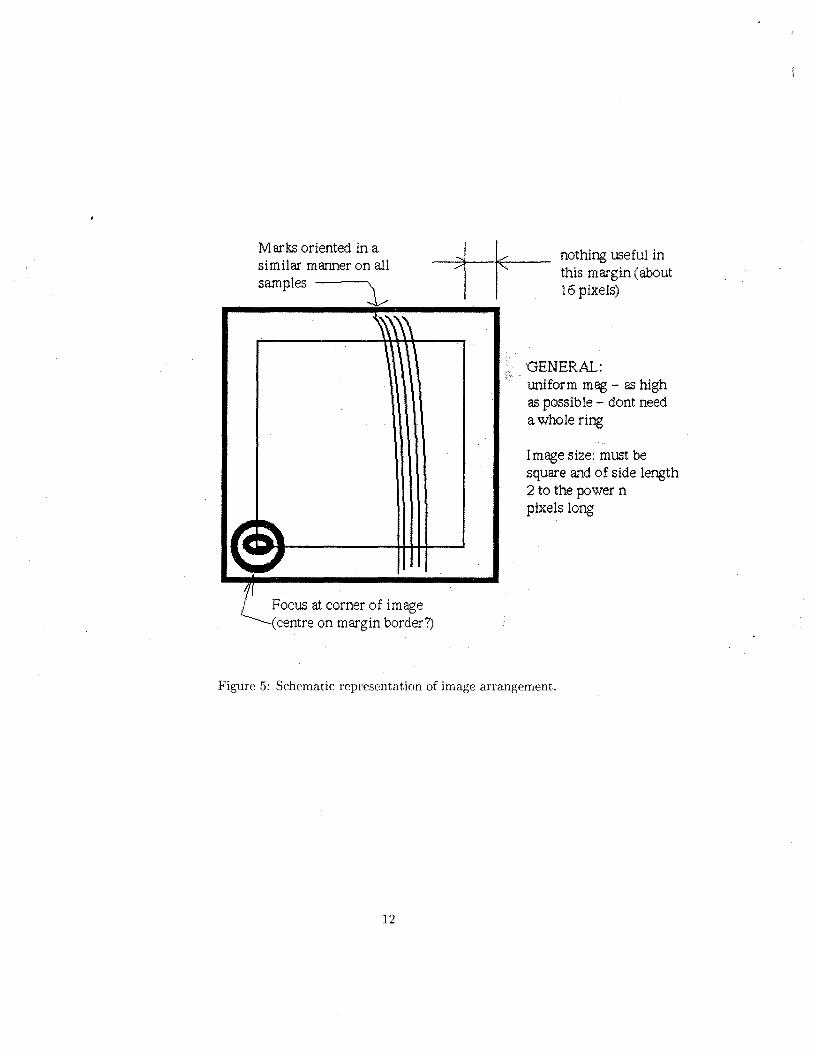
Marks oriented in a similar manner on all samples

Focus at corner of image centre on margin border?)

nothing useful in this margin (about 16 pixels)

'GENERAL: uniform mag - as high as possible - dont need a whole ring

I mage size: must be square and of side length 2 to the power n pixels long

Figure 5: Schematic representation of image arrangement.

12

(e) (f) (g) (h)

Figure 6: Pairs of input and output images. Images (a)-(d) are from wild fish and images (e)-(h) are from thermally marked fish

13