University of Central Florida University of Central Florida

STARS STARS

Electronic Theses and Dissertations, 2004-2019

2007

Discussion On Effective Restoration Of Oral Speech Using Voice Discussion On Effective Restoration Of Oral Speech Using Voice

Conversion Techniques Based On Gaussian Mixture Modeling Conversion Techniques Based On Gaussian Mixture Modeling

Gustavo Alverio University of Central Florida

Part of the Electrical and Electronics Commons

Find similar works at: https://stars.library.ucf.edu/etd

University of Central Florida Libraries http://library.ucf.edu

This Masters Thesis (Open Access) is brought to you for free and open access by STARS. It has been accepted for

inclusion in Electronic Theses and Dissertations, 2004-2019 by an authorized administrator of STARS. For more

information, please contact STARS@ucf.edu.

STARS Citation STARS Citation Alverio, Gustavo, "Discussion On Effective Restoration Of Oral Speech Using Voice Conversion Techniques Based On Gaussian Mixture Modeling" (2007). Electronic Theses and Dissertations, 2004-2019. 3060. https://stars.library.ucf.edu/etd/3060

DISCUSSION ON EFFECTIVE RESTORATION OF ORAL SPEECH USING VOICE CONVERSION TECHNIQUES BASED ON

GAUSSIAN MIXTURE MODELING

by

GUSTAVO ALVERIO B.S.E.E. University of Central Florida, 2005

A thesis submitted in partial fulfillment of the requirements for the degree of Master of Science

in the School of Electrical Engineering and Computer Science in the College of Engineering and Computer Science

at the University of Central Florida Orlando, Florida

Summer Term 2007

Major Professor: Wasfy B. Mikhael

ii

ABSTRACT

Today’s world consists of many ways to communicate information. One of

the most effective ways to communicate is through the use of speech.

Unfortunately many loose the ability to converse. This in turn leads to a large

negative psychological impact. In addition, skills such as lecturing and singing

must now be restored via other methods.

The usage of text-to-speech synthesis has been a popular resolution of

restoring the capability to use oral speech. Text to speech synthesizers convert

text into speech. Although text to speech systems are useful, they only allow for

few default voice selections that do not represent that of the user. In order to

achieve total restoration, voice conversion must be introduced.

Voice conversion is a method that adjusts a source voice to sound like a

target voice. Voice conversion consists of a training and converting process.

The training process is conducted by composing a speech corpus to be spoken

by both source and target voice. The speech corpus should encompass a variety

of speech sounds. Once training is finished, the conversion function is employed

to transform the source voice into the target voice. Effectively, voice conversion

allows for a speaker to sound like any other person. Therefore, voice conversion

can be applied to alter the voice output of a text to speech system to produce the

target voice.

iii

The thesis investigates how one approach, specifically the usage of voice

conversion using Gaussian mixture modeling, can be applied to alter the voice

output of a text to speech synthesis system. Researchers found that acceptable

results can be obtained from using these methods. Although voice conversion

and text to speech synthesis are effective in restoring voice, a sample of the

speaker before voice loss must be used during the training process. Therefore it

is vital that voice samples are made to combat voice loss.

iv

ACKNOWLEDGMENTS

I would like to give special thanks to my advisor Dr. Wasfy Mikhael for his

perseverance in assisting me throughout my graduate career, and never

doubting my ability to finish. I wish to also give thanks to Dr. Alexander Kain of

the Center for Spoken Language Understanding for providing the breakthrough

opportunity in beginning my research. I would like to attach importance to the

Electrical Engineering department, and AT&T Labs for their tools in allowing me

to complete my work. Last but not least, I thank my family and friends for their

never-ending support during the study of this thesis.

v

TABLE OF CONTENTS

LIST OF FIGURES .............................................................................................viii

LIST OF TABLES ................................................................................................. x

LIST OF ACRONYMS ..........................................................................................xi

CHAPTER 1: INTRODUCTION........................................................................... 1

1.1 Motivation.................................................................................................... 1

1.2 Fundamentals of Speech ............................................................................ 3

1.2.1 The Levels of Speech........................................................................... 4

1.2.2 Source Filter Model .............................................................................. 5

1.2.3 Graphical Interpretations of Speech Signals ........................................ 8

1.3 Organization of Thesis .............................................................................. 10

CHAPTER 2: VOICE CONVERSION SYSTEMS .............................................. 12

2.1 Phases of Voice Conversion ..................................................................... 12

2.1.1 Training .............................................................................................. 13

2.1.2 Converting .......................................................................................... 14

2.2 Varieties of Voice Conversion Systems .................................................... 14

2.2.1 Voice Conversion Using Vector Quantization..................................... 15

2.2.2 Voice Conversion Using Artificial Neural Networks ............................ 17

2.3 Applying Voice Conversion to Text To Speech Synthesis......................... 18

CHAPTER 3: TEXT TO SPEECH SYNTHESIS ................................................ 20

vi

3.1 From Mechanical to Electrical Speech Synthesizers ................................ 20

3.2 Concatenated Synthesis ........................................................................... 24

3.3 Challenges Encountered........................................................................... 26

3.4 Advantages of Synthesizers...................................................................... 27

CHAPTER 4: VOICE CONVERSION USING GAUSSIAN MIXTURE MODELING

........................................................................................................................... 29

4.1 Gaussian Mixture Models.......................................................................... 29

4.2 Choosing GMM for Conversion................................................................. 31

4.3 Establishing the Features for Training ...................................................... 34

4.3.1 The Bark Scale................................................................................... 34

4.3.2 LSF Computation ............................................................................... 36

4.4 Mapping Using GMM ................................................................................ 40

4.5 Developing the Conversion Function for Vocal Tract Conversion ............. 42

4.6 Converting the Fundamental Frequency F0.............................................. 44

4.6.1 Defining F0 ......................................................................................... 45

4.6.2 Extracting F0 ...................................................................................... 46

4.7 Rendering the Converted Speech............................................................. 48

CHAPTER 5: EVALUATIONS ........................................................................... 50

5.1 Subjective Measures of Voice Conversion Processes .............................. 50

5.1.1 Vector Quantization Results ............................................................... 51

5.1.2 Voice Conversion using Least Squares GMM .................................... 53

5.1.3 Results of GMM Conversion of Joint Space ....................................... 57

vii

5.2 Objective Measure of Voice Conversion Processes ................................. 59

5.2.1 Results of using Neural Networks in voice conversion ....................... 60

5.2.2 VQ Objective Results ......................................................................... 62

5.2.3 GMM Using Least Squares Objective Results.................................... 62

5.2.4 Joint Density GMM Voice Conversion Results ................................... 64

5.2.5 Pitch Contour Prediction..................................................................... 65

CHAPTER 6: DISCUSSIONS............................................................................ 67

6.1 Introducing the Method to Solve Current Problems .................................. 67

6.2 Challenges Encountered........................................................................... 70

6.3 Future work ............................................................................................... 71

CHAPTER 7: CONCLUSIONS .......................................................................... 74

REFERENCES................................................................................................... 76

viii

LIST OF FIGURES

Figure 1: Linear system of the Source Filter model. ............................................ 6

Figure 2: The linear system representation of (a) the LPC process and (b) the

Source Filter model.................................................................................... 7

Figure 3: Time waveform representation of speech............................................. 8

Figure 4: Fourier transforms of [a] (top) and [ʃ] (bottom) from the French word

baluchon [1]. .............................................................................................. 9

Figure 5: Spectrogram of the spoken phrase “taa baa baa.” ............................. 10

Figure 6: Flow diagram of voice conversion with phase indication. ................... 13

Figure 7: Training of voice conversion using vector quantization. ..................... 16

Figure 8: Conversion phase using vector quantization. ..................................... 17

Figure 9: Wheatstone’s design of the von Kempelen talking machine [11]......... 22

Figure 10: Texas Instruments’ Speak & Spell popularized text to speech

systems.................................................................................................... 24

Figure 11: The processes in text to speech transcription. ................................. 25

Figure 12: The clustering of data points using GMM with prior probabilities...... 30

Figure 13: Distortion between converted and target data (stars) and converted

and source data (circles) for different sizes of (a) GMM and (b) VQ method

[17]........................................................................................................... 32

Figure 14: Magnitude response of )(zP and )(zQ [25]. ..................................... 40

ix

Figure 15: The mapping of the joint speaker acoustic space through GMM [29].

................................................................................................................. 42

Figure 16: The excitation for a typical voiced sound [25]................................... 45

Figure 17: The excitation for a typical unvoiced sound [25]. .............................. 46

Figure 18: The voiced waveform with periodic traits [32]. .................................. 47

Figure 19: The autocorrelation values of Figure 18 [32]. ................................... 47

Figure 20: Normalized cepstrum of the voiced /i/ in “we were” [33]. .................. 48

Figure 21: Manipulating the F0 by means of PSOLA techniques [10]. .............. 49

Figure 22: Space representation of listening test results for male to female

conversion using VQ [8]........................................................................... 52

Figure 23: Opinion test results of source speaker GMM with the Least Squares

technique [28]. ......................................................................................... 56

Figure 24: Formant sequence of /a/ to /e/ for transformation of source (top), and

the target speaker (bottom) [9]................................................................. 61

Figure 25: Spectral distortion measures as a function of mixture number of

converted and target spectral envelope [28]. ........................................... 63

Figure 26: Spectral envelope of source (dotted), converted(dashed), and

target(solid) using 128 mixtures [28]. ....................................................... 64

Figure 27: Normalized error for Least Squares and Joint Density GMM voice

conversion [6]. ......................................................................................... 65

Figure 28: The overall voice restorer. ................................................................ 68

x

LIST OF TABLES

Table 1: Properties of LSFs. .............................................................................. 34

Table 2: Corresponding frequencies of Bark values. ......................................... 35

Table 3: Experiment 1 tests for male to female VQ conversion. ........................ 52

Table 4: ABX evaluated results for male to male VQ conversion. ..................... 53

Table 5: Training sets for LSF Joint GMM conversion....................................... 58

Table 6: Subjective results of Joint GMM conversion. ....................................... 58

Table 7: Formant percentage error before and after neural network conversion.

................................................................................................................. 60

Table 8: Spectral distortions of the VQ method. ................................................ 62

Table 9: Pitch contour prediction errors............................................................. 66

xi

LIST OF ACRONYMS

EM Expectation Maximization

F0 Fundamental frequency

FFT Fast Fourier Transform

GMM Gaussian Mixture Model

LPC Linear Predictive Coding

LSF Line Spectral Frequencies

PSOLA Pitch Synchronous Overlap and Add

MATLAB MATrix LABoratory program

MOS Mean Opinion Scores

TTS Text To Speech

VODER Voice Operating Demonstrator

VQ Vector Quantization

1

CHAPTER 1: INTRODUCTION

Restoration of speech involves many aspects of the science and

engineering fields. Topics to study in the restoration process include speech

science, statistics, and signal processing. Speech science provides the

knowledge of the formation of voice. Statistics help to model the characterization

of spectral features. Also, signal processing provides the techniques to produce

voices using mathematics. When combining the knowledge of these areas, the

complexity of voice restoration can be fully understood and solved.

1.1 Motivation

A fast effective method to express ideas and knowledge is through the use

of oral speech. The actor can use his or her voice to help explain the story that

people are watching. The salesperson describes the product to the purchaser

orally. The singer belts the lyrics of the song with its powerful vocals. All are

common examples of when people use their verbal skills. Now consider the

following examples. An actor perishes before the completion of the animated

television series or movie that he/she was starring. Laryngitis affects a

telemarketer shortly before the start of the workday. The singer finds out that

soon he or she will undergo throat surgery, with unavoidable damage to oral

communication.

2

Each of these scenarios involve one similar problem; that each person

loses the ability to communicate vocally. What makes this problem even more

complex is that without oral speech, each person must now rely on other means

to maintain their previous occupations. Unfortunately however, what other

means do they have to continue normality? How do the producers continue with

the movie without their leading actor? Will the telemarketer suffer slow sales

now that speech can no longer be used? Can the singer preserve his or her

flourishing singing career?

One possible solution to restoring the voices in people is by employing

text to speech synthesis. Text to speech synthesis enables an oral presentation

of text. These synthesizers follow grammatical rules to produce the vocal sound

equivalent of the text being “read”. The sounds are created from recording

human sound pronunciations. Each sound is then concatenated together to

produce the word orally. Sound recording however is a lengthy and precise

procedure. In addition, the overall output yields a foreign voice unlike that of

people whom have lost their voice.

Therefore, text to speech synthesis cannot solely be used to resolve the

examples stated. Instead, by integrating a text to speech synthesizer along with

voice conversion, the overall system will achieve the voice that was lost. In

essence, voice conversion implies that one voice is modified to sound like a

different voice. By identifying the parameters of any voice, those parameters can

be altered to mimic the voice of the people in the aforementioned examples. If

3

voice conversion techniques are integrated, it will help allow the producers to

premiere their movie to the public audience, guarantee a profit for the

telemarketer’s earnings, and enable the singer to record multi-platinum songs.

Although the concept is fundamentally simplistic, human speech is

unfortunately complex, resulting in fairly intricate methodology. The complexity

arises because people speak with varying dialects of the same language,

accents, and at times even alter their own pronunciation of the same sound.

These complexities in human speech presents added challenges for voice

conversion techniques.

These challenges require further studying in speech processing.

Numerous institutions are providing proposals for research in voice conversion

because of the benefit it can impart on millions of people. The increase in grants

for voice conversion research requires a demand for more students. Students

seeking a rich and substantial graduate thesis can be greatly rewarded by

focusing their studies in the field of speech processing in voice conversion.

1.2 Fundamentals of Speech

In order to understand the techniques discussed in this thesis, the

fundamentals of speech must first be introduced. Speech can be broken down to

various levels such as the acoustic, phonetic, phonological, morphological,

syntactic, semantic, and pragmatic as defined in [1]. The most mentioned levels

will be the acoustic, phonetic, and phonological. Topics such as the source filter

4

model and graphical interpretations of speech are also fully analyzed to provide

additional solid comprehension of the terms and techniques used for the thesis

study. The section on the Source Filter model will provide answers to questions

such as how speech is produced, and how can speech be modeled. Finally a

section on graphical interpretations of speech signals will allow the reader to

understand how to read the graphs provided throughout the thesis.

1.2.1 The Levels of Speech

The acoustic level defines the speech to be developed when the

articulatory system experiences a change in air pressure, and is comprised of

three aspects, the fundamental frequency, intensity and the spectral energy

distribution which signifies the pitch, loudness, and timbre respectively. These

three aspects are obtained when transforming the speech signal into an electrical

signal using a microphone. After attaining the electrical signal, digital signal

processing techniques can then be used to extract the three traits.

The phonetic level begins the introduction of the phonetic alphabet. The

phonetic alphabet represents pronunciation breakdowns for various sounds.

Each language has a unique phonetic alphabet. The phonological level then

interprets the phonetic alphabet to phonemes. Phonemes represent a functional

unit of speech. This is the level that bridges the phonetics to higher-level

linguistics. The combination of phonemes can then be interpreted to the

morphological level, where words can be formed and studied based on stems

5

and affixes. Syntax restricts the formulations of sentences. The syntax level

helps to reduce the number of sentences possible. The semantic level is an

additional level to help shape a meaningful sentence. This level is needed

because the syntax is not an acceptable criterion for languages. Semantics is

the study of how words are related to one another. Pragmatics is an area that

encompasses presuppositions and indirect speech acts.

The levels strongly associated with this thesis are the acoustic, phonetic,

and phonological. These levels help describe the sounds that allow for speech

development. The other levels only constitute the comprehension of speech,

which is controlled by the input of the user, and therefore does not need to be

studied further.

1.2.2 Source Filter Model

Speech is the result of airflow, vibrations of the vocal cords, and blockage

of the airflow due to the mouth. Organically, the airflow provides the excitation

needed for the vocal cords to shape the excitation into a phoneme. This results

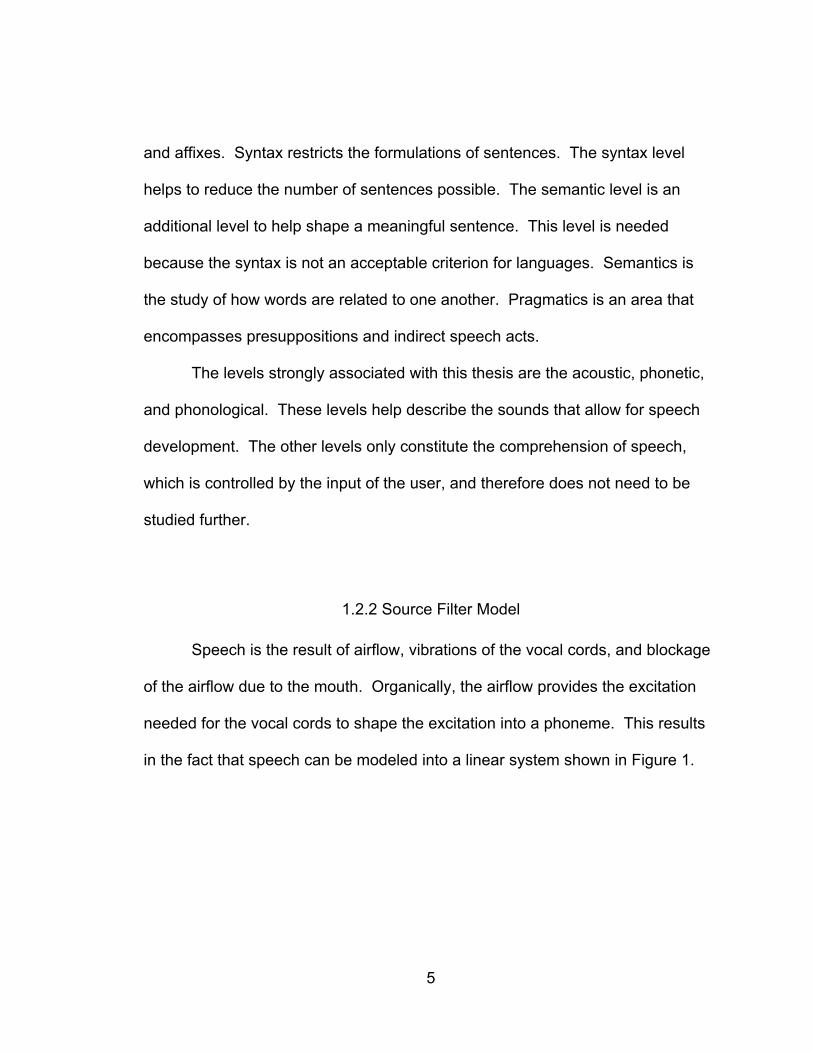
in the fact that speech can be modeled into a linear system shown in Figure 1.

6

Figure 1: Linear system of the Source Filter model.

The method of looking at speech as two distinct parts that can be

separated is known as the Source Filter model of speech [2]. The Source Filter

model consists of the transfer function and the excitation. The transfer function

contains the vocal tract. The excitation contains the pitch and sound. The

excitation, or the source, can either be voiced or unvoiced. Voiced sounds

include vowels and indicate a vibration in the vocal cords. Unvoiced sounds

mimic noise and have no oscillatory components. Examples of unvoiced

phonemes include /p/, /t/, and /k/.

In order to apply the Source Filter model, first assume that the n th sample

of speech is predicted by the past p samples such that

.)()(ˆ1∑=

−=p

ii insans (1)

Then an error signal can define the error between the actual and predicted

signals. This error can be expressed as

.)()()(ˆ)()(1∑=

−−=−=p

ii insansnsnsnε (2)

Voiced sounds

Unvoiced Sounds

Vocal tract

Output speech

7

The goal is to minimize the error signal, so that the predicted signal matches the

actual signal. The task of minimizing )(nε is to find the ia s, which can be done

using an autocorrelation or covariance method. Now the error signal defined in

(2) can be found. Next the z -transform of (2) is taken to produce

.)()(1)()()()(11

zAzSzazSzzSazSzEp

i

ii

p

i

ii =⎥

⎦

⎤⎢⎣

⎡−=−= ∑∑

=

−

=

− (3)

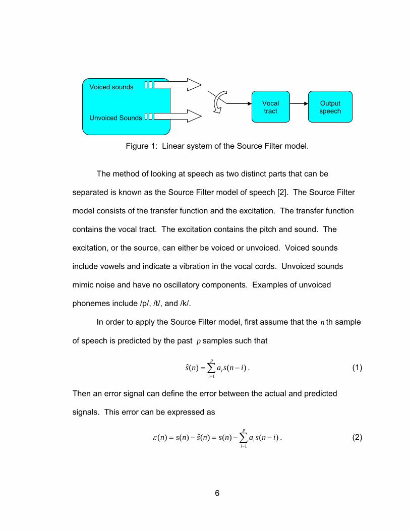
The results of (3) produces two linear systems that describe the Linear Prediction

Coding (LPC) process and the Source Filter model shown in Figure 2a and

Figure 2b respectively.

Figure 2: The linear system representation of (a) the LPC process and (b) the

Source Filter model.

Speech signals can be encoded using LPC based on the Source Filter

model. LPC is used to analyze speech signals )(ns by first estimating the

formants with the filter )(zA [3]. The formants are the peaks of the spectral

)(nε )(1zA )(ns

)(ns

)(zA )(nε

(a)

(b)

8

envelopes of which pertain to the vocal tract filter indicated by )(

1zA

. Then the

effects of the formants are removed to estimate the source signal )(nε . The

remaining signal is also called the residue.

The formants can be determined from the speech signal that is described

by Equation 1 is called a linear predictor, hence the term Linear Prediction

Coding. The coefficients ia of the linear predictor characterize the formants of

the spectral envelope. These coefficients are estimated by reducing the mean-

squared error of Equation 2.

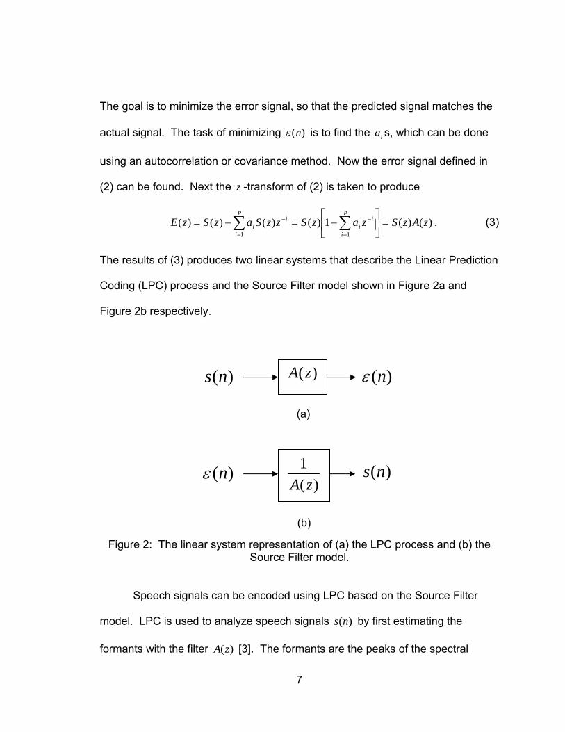
1.2.3 Graphical Interpretations of Speech Signals

There are two basic waveforms to represent speech signals. Figure 3

represents a time waveform of a speech signal. The horizontal axis indicates

time while the vertical axis indicates amplitude of the signal, which can be

inferred as the loudness. The only visible information that can be extracted from

this type of graph is when silences and spoken speech occurs.

Figure 3: Time waveform representation of speech.

9

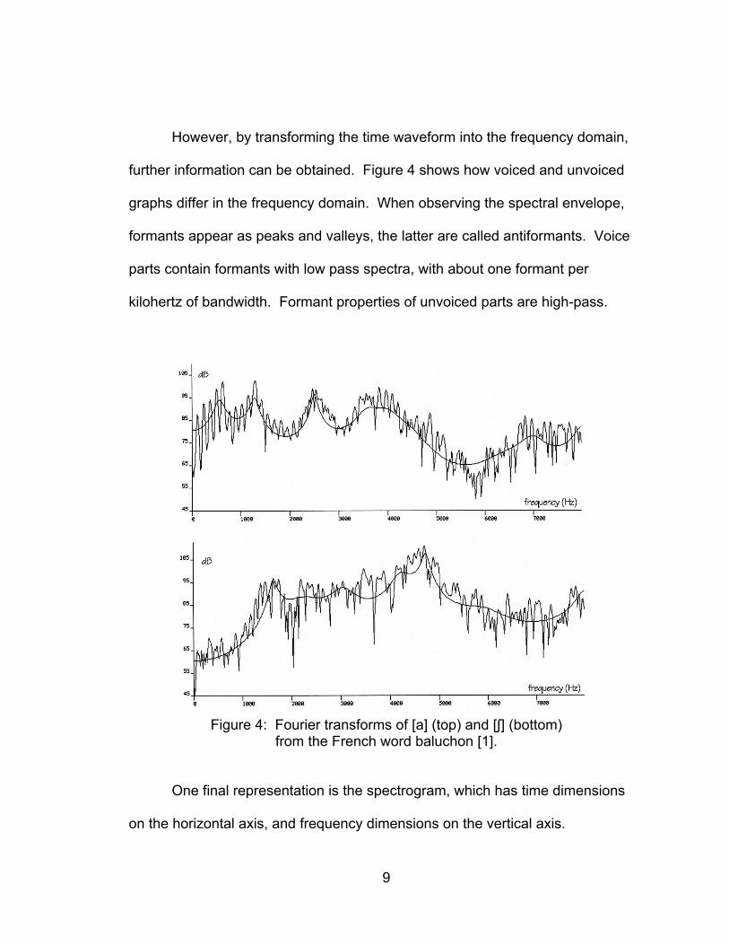
However, by transforming the time waveform into the frequency domain,

further information can be obtained. Figure 4 shows how voiced and unvoiced

graphs differ in the frequency domain. When observing the spectral envelope,

formants appear as peaks and valleys, the latter are called antiformants. Voice

parts contain formants with low pass spectra, with about one formant per

kilohertz of bandwidth. Formant properties of unvoiced parts are high-pass.

Figure 4: Fourier transforms of [a] (top) and [ʃ] (bottom)

from the French word baluchon [1].

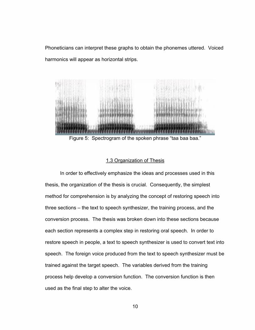
One final representation is the spectrogram, which has time dimensions

on the horizontal axis, and frequency dimensions on the vertical axis.

10

Phoneticians can interpret these graphs to obtain the phonemes uttered. Voiced

harmonics will appear as horizontal strips.

Figure 5: Spectrogram of the spoken phrase “taa baa baa.”

1.3 Organization of Thesis

In order to effectively emphasize the ideas and processes used in this

thesis, the organization of the thesis is crucial. Consequently, the simplest

method for comprehension is by analyzing the concept of restoring speech into

three sections – the text to speech synthesizer, the training process, and the

conversion process. The thesis was broken down into these sections because

each section represents a complex step in restoring oral speech. In order to

restore speech in people, a text to speech synthesizer is used to convert text into

speech. The foreign voice produced from the text to speech synthesizer must be

trained against the target speech. The variables derived from the training

process help develop a conversion function. The conversion function is then

used as the final step to alter the voice.

11

Chapter 2 is used to familiarize the reader about voice conversion before

covering the training and conversion sections. The first section, the text to

speech synthesis, is exclusively discussed in Chapter 3. Chapter 3 will examine

in-depth the science behind text to speech synthesis. Chapter 4 begins the

explanation of the theory of the final two sections, the training and converting

process. Evaluations of the results from studies are addressed in Chapter 5.

Chapter 6 provides a discussion on the restoration of voice with future ideas and

problems confronted.

12

CHAPTER 2: VOICE CONVERSION SYSTEMS

Voice conversions systems can provide for many beneficial solutions to

current voice loss problems. Unlike voice modification, where speech sounds

are simply transformed to create a unique sound, voice conversion is created

from a specific set of changes required to mimic the voice of another. These

changes mostly are based on the spectral mapping methods between a source

and target speaker. Conversion systems can differ based on their statistical

mapping and their conversion function. Some conversion systems use mapping

codebooks, discrete transformation functions, artificial neural networks, Gaussian

mixture models (GMM), or a combination of some of them [4].

2.1 Phases of Voice Conversion

The basic objective of all voice conversion systems is to modify the source

speaker so that it is perceived to sound like a target speaker [5]. In order to

execute the proper modification, the voice conversion system must follow specific

phases. Each voice conversion system has two key phases, a training phase

and a conversion phase. Figure 6 represents a flow chart of the typical voice

conversion system.

13

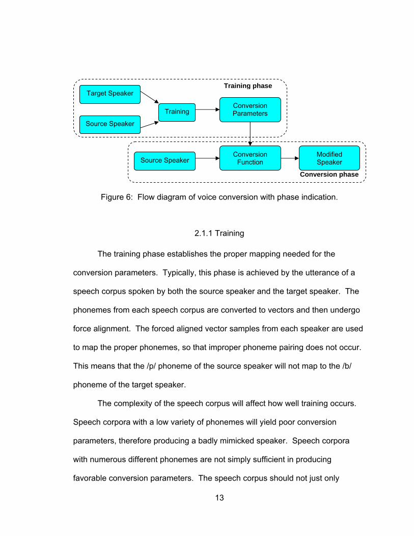
Figure 6: Flow diagram of voice conversion with phase indication.

2.1.1 Training

The training phase establishes the proper mapping needed for the

conversion parameters. Typically, this phase is achieved by the utterance of a

speech corpus spoken by both the source speaker and the target speaker. The

phonemes from each speech corpus are converted to vectors and then undergo

force alignment. The forced aligned vector samples from each speaker are used

to map the proper phonemes, so that improper phoneme pairing does not occur.

This means that the /p/ phoneme of the source speaker will not map to the /b/

phoneme of the target speaker.

The complexity of the speech corpus will affect how well training occurs.

Speech corpora with a low variety of phonemes will yield poor conversion

parameters, therefore producing a badly mimicked speaker. Speech corpora

with numerous different phonemes are not simply sufficient in producing

favorable conversion parameters. The speech corpus should not just only

Source Speaker

Target Speaker

Training Conversion Parameters

Source Speaker Conversion

Function Modified Speaker

Training phase

Conversion phase

14

include many different phonemes, but repetition of phonemes that can help mold

an affective copy of the target speaker.

2.1.2 Converting

The conversion parameters computed during the training process are

used to develop the conversion function. The goal of the conversion function is

to minimize the mean squared error between the target speaker and the modified

speaker based on the source speaker. The conversion function can be

implemented using mapping codebooks, dynamic frequency warping, neural

networks, and Gaussian mixture modeling [6]. Depending on the method used,

the vectors of the source are inputted into the function for conversion. The

predicted target vectors indicate the spectral parameters of the new voice. The

pitch of the speaker’s residual is adjusted to match the target speaker’s pitch in

average value and variance. Both the spectral parameters and the modified

residual are then convolved to form the new modified voice [7].

2.2 Varieties of Voice Conversion Systems

The training process can be completed using various methods. One

method is called the vector quantization method. Vector quantization is a

method to lower the dimensional space by using codebooks. The source and

target speaker vectors are converted to codebooks that carry all acoustical traits

15

of each speaker. Now, instead of mapping the speakers, the codebooks are

mapped [8]. The other method employs artificial neural networks to perform the

mapping [9]. This method uses the formants for transformation. The method of

using Gaussian mixture models will be discussed in detail in Chapter 4.

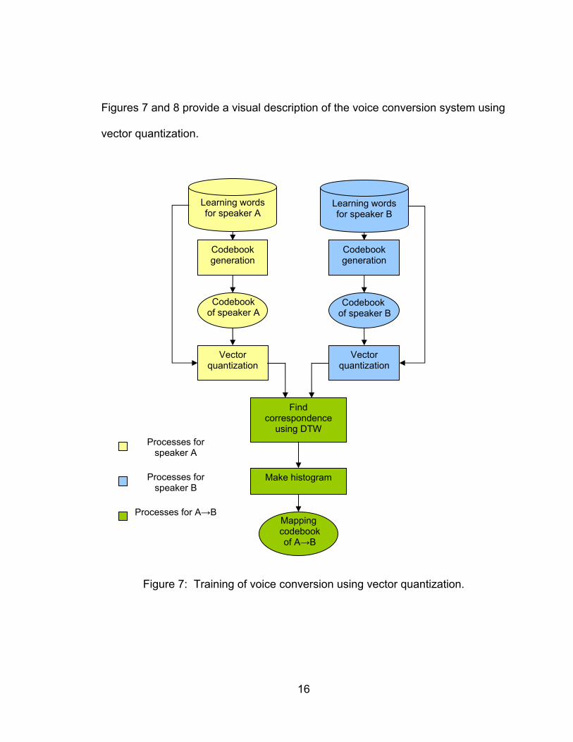
2.2.1 Voice Conversion Using Vector Quantization

The vector quantized method maps the spectral parameters, the pitch

frequencies, and the power values. The spectral parameters are mapped first by

having each speech corpus vector quantized (coded) by words. Then the

correspondence of the same words are determined using dynamic time warping

– a method of force alignment. All correspondences are accumulated into a

histogram which acts as the weighting function for the mapping codebooks. The

mapping codebooks are defined as a linear combination of the target vector.

The pitch frequencies and the power values are mapped similarly to the

spectral parameters except that one, both pitch frequencies and power values

are scalar quantized, and two, pitch frequencies use the maximum occurrence in

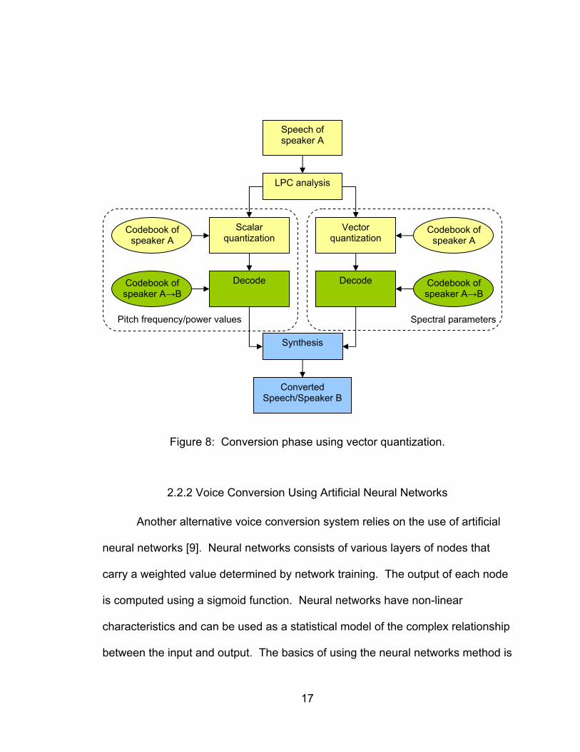
the histogram for the mapping codebook. The conversion phase using vector

quantization first begins with the utterance of the source speaker. The voice is

analyzed using LPC. The spectrum parameters and pitch frequencies/power

values obtained are vector quantized and scalar quantized respectively using the

target codebooks generated during training. The decoding is carried out by using

the mapping codebooks to ultimately produce the voice of the target speaker.

16

Figures 7 and 8 provide a visual description of the voice conversion system using

vector quantization.

Figure 7: Training of voice conversion using vector quantization.

Processes for speaker B

Codebook generation

Vector quantization

Learning words for speaker B

Learning words for speaker A

Codebook generation

Vector quantization

Find correspondence

using DTW

Make histogram

Codebook of speaker A

Codebook of speaker B

Mapping codebook of A→B

Processes for speaker A

Processes for A→B

17

Figure 8: Conversion phase using vector quantization.

2.2.2 Voice Conversion Using Artificial Neural Networks

Another alternative voice conversion system relies on the use of artificial

neural networks [9]. Neural networks consists of various layers of nodes that

carry a weighted value determined by network training. The output of each node

is computed using a sigmoid function. Neural networks have non-linear

characteristics and can be used as a statistical model of the complex relationship

between the input and output. The basics of using the neural networks method is

Pitch frequency/power values

Decode Decode

Synthesis

Converted Speech/Speaker B

LPC analysis

Scalar quantization

Speech of speaker A

Vector quantization

Codebook of speaker A

Codebook of speaker A→B

Codebook of speaker A→B

Codebook of speaker A

Spectral parameters

18

that a feed forward neural network is trained using the back propagation method

to yield a function that transforms the formants of the source speaker to those of

the target speaker.

For the study in [9], the results indicated that the transformation of the

vocal tract between two speakers is not linear. Because of its nonlinear

properties, the neural network was proposed for formant transformation. In order

to train the neural network, a discrete set of points on the mapping function is

used. If the set of points are correctly identified, the network will learn a

continuous mapping function that can even transform input parameters that were

not originally used for training. The properties of neural networks also avoid the

use of large codebooks. The neural network described consists of one input

layer with three nodes, two hidden layers of eight nodes each, and a three node

output layer. The basic algorithm for training consists of using the three formant

values of the source as input. Then the desired outputs are the formants

extracted by the corresponding target. The weights are computed using the back

propagation method. This three step process is repeated until the weights

converge.

2.3 Applying Voice Conversion to Text To Speech Synthesis

The knowledge gained from voice conversion can be applied to text to

speech synthesis for a solution to voice loss. If the source speaker is that of the

output of the text to speech software, then the text to speech software will utter

19

phrases in the same voice as the target speaker. Therefore, the text to speech

software can be used to produce the voice of the target speaker assuming that

training can be done with a sample of the target speaker. Another additional

feature of using a text to speech system as the source output is that the user will

no longer be dependant on others for speech production. Instead, the user can

type the desired message in the text to speech.

20

CHAPTER 3: TEXT TO SPEECH SYNTHESIS

Origins of synthesizers were adapted from mechanical to electrical means.

It is important to note the specific type of system discussed in this thesis. Most

agree that text to speech synthesizers are mostly focused on the ability to

automatically produce new sentences electrically, regardless of the language [1].

Text to speech synthesizers may vary according to their linguistic formalisms.

Like many new advances in technology, text to speech synthesis has its share of

challenges. Fortunately, there are many advantages of using this type of

technology.

3.1 From Mechanical to Electrical Speech Synthesizers

Speech synthesizers have come a long way since the early versions. The

history of synthesizers for speech began in 1779 when Russian Professor

Christian Kratzenstein made a mechanical apparatus to produce the vowels /a/,

/e/, /i/, /o/, and /u/ artificially [10]. These mechanical designs acted much like

musical instruments. The acoustic resonators were activated by blowing into the

vibrating reeds. These reeds function similarly to instruments such as clarinets,

saxophones, bassoons, and oboes. Kratzenstein helped pave the way for further

studies into mechanical speech production.

21

Following Kratzenstein’s inventions, Wolfgang von Kempelen introduced

the “Acoustic-Mechanical Speech Machine.” This invention took the artificial

vowel apparatus a step further. Instead of producing single phoneme sounds,

von Kempelen’s machine allowed for some sound combinations. Von

Kempelen’s machine was composed of a pressure chamber to act as the lungs,

a vibrating reed to mimic the vibrations of the vocal cords, and a leather tube to

portray the vocal tract.

Much like Kratzenstein’s machine, von Kempelen’s machine required

human stimulus for operation. Unlike Kratzenstein’s machine, the air for the

system was provided by the compression of the bellows. Bending the leather

tube would allow different vowels to be produced. Consonants were achieved by

finger constriction of the four passages. Plosives sounds were generated using

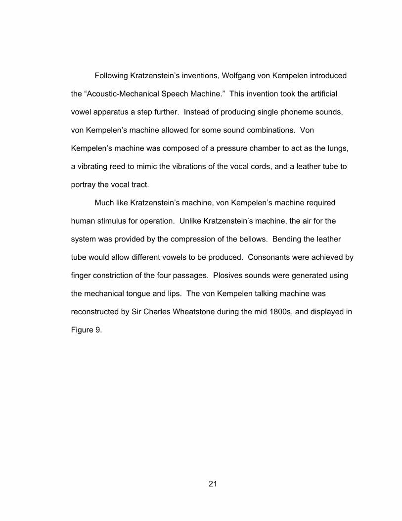
the mechanical tongue and lips. The von Kempelen talking machine was

reconstructed by Sir Charles Wheatstone during the mid 1800s, and displayed in

Figure 9.

22

Figure 9: Wheatstone’s design of the von Kempelen talking machine [11].

It is interesting to note that much more precise human involvement is

required when using the von Kempelen method [11]. The right upper arm

operated the bellows while the nostril openings, reed bypass, and whistle levers

were controlled with the right hand. The left hand controlled the leather tube.

Von Kempelen stated that 19 consonants sound could be produced by the

machine, although the quality of the voice may depend on who was listening.

Through the study of the machine, von Kempelen theorized that the vocal tract

was the main source of acoustics, which contradicted the previous belief that the

larynx was the main source.

Scientists started electrical synthesis during the 1930s in hopes of

performing automatic synthesis. The first advancement of electrical synthesizers

is considered to be the Voice Operating Demonstrator, or VODER [12].

23

Introduced by Homer Dudley, the synthesizer required skillful tact much like the

von Kempelen machine.

The next major advancement of electrical synthesis was in 1960 when

speech analysis and synthesis techniques were divided into system and signal

approaches referred to in [13], with the latter approach focusing on reproducing

the speech signal. The system approach is also termed articulatory synthesis,

while the signal approach is termed terminal-analogue synthesis. The signal

approach helped give berth to the formant and linear predictive synthesizers.

Articulatory synthesizers were first introduced in 1958, with a full scale text to

speech system for English developed by Noriko Umeda in 1968 based on this

type of synthesis [14]. With the development by Umeda, commercial text to

speech synthesis became a popular area of research. The 1970s and 80s

provided the first integrated circuit based on formant synthesis.

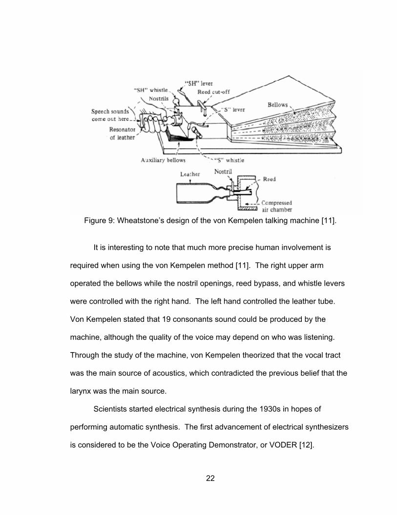
A popular invention came about during 1980 under the title of Speak &

Spell from Texas Instruments, imaged in Figure 10. This electronic reading aid

for children is based on the linear prediction method of speech synthesis.

24

Figure 10: Texas Instruments’ Speak & Spell popularized text to speech

systems.

3.2 Concatenated Synthesis

Most typical systems use concatenative processes that consist of

combining an assortment of sounds to create the equivalent translation from text

to vocals. The concatenation provided during transcription is diverse. Some

systems concatenate phonemes while other systems concatenate whole words.

The functionality of the synthesizers relies greatly on the databases

provided for concatenation. Synthesizers used in airports require a verbalization

of the time and date. These systems therefore must be able to speak numbers

and months. Therefore a rather small database is required for this type of utility.

However, reading e-mails, which is one use of text to speech systems, will result

in an extremely large database.

25

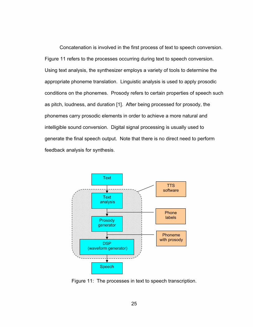
Concatenation is involved in the first process of text to speech conversion.

Figure 11 refers to the processes occurring during text to speech conversion.

Using text analysis, the synthesizer employs a variety of tools to determine the

appropriate phoneme translation. Linguistic analysis is used to apply prosodic

conditions on the phonemes. Prosody refers to certain properties of speech such

as pitch, loudness, and duration [1]. After being processed for prosody, the

phonemes carry prosodic elements in order to achieve a more natural and

intelligible sound conversion. Digital signal processing is usually used to

generate the final speech output. Note that there is no direct need to perform

feedback analysis for synthesis.

Figure 11: The processes in text to speech transcription.

Text

Text analysis

Prosody generator

DSP (waveform generator)

Speech

Phone labels

Phoneme with prosody

TTS software

26

3.3 Challenges Encountered

There are many challenges for text to speech systems. As high quality

text to speech synthesis became more and more popular, researchers began to

analyze the impact in society of such technologies. As noted in [15], the

“Acceptance of a new technology by the mass market is almost always a function

of utility, usability, and choice. This is particularly true when using a technology

to supply information where the former mechanism has been a human.” The

main importance of utility refers to financial cost of using and producing such

systems. Certain text to speech systems require large databases and complex

modeling that can increase cost production. The usability is also a challenge.

Although speech is intelligible, it is still limited to the lack of emotional emphasis.

Stereotypical views of synthesizers are that they sound robotic and overall are

inefficient to be introduced into societal practices.

Another challenge to text to speech synthesis is pronunciation, which

occurs when the system is “reading.” Although some languages, like Spanish,

contain regular pronunciation rules, other languages, like English, contain many

irregular pronunciations. For example, the English pronunciation of the phoneme

/f/ will differ when referring to the word “of,” in which the /f/ is pronounced more

like /v/. These irregular pronunciations can also be discovered in the alternate

spelling of “fish” as “ghoti.” The /gh/ indicates the ending of the word “tough,” the

/o/ is pronounced similarly to the /o/ in “women,” and finally the /ti/ is spoken like

in the word “fiction.”

27

Pronunciation of numbers is also problematic. There are various ways to

pronounce the numbers 3421. While the simple synthesis of “three four two one”

may be practical for reading social security numbers or sequence of numbers, it

is simply not practical for all occasions. One occasion can refer to the “number

three thousand four hundred twenty-one,” while another may need to imply the

address of a house such as “thirty-four twenty-one.”

Other pronunciation hazards are common in the form of abbreviations and

acronyms. Some abbreviations such as the units for inches (in.) form a word in

itself, relying on the system to know the correct understanding of when the

proper pronunciation must be used. Acronyms cause databases to become

greatly complex. As in the case of the pronunciation of the virus AIDS, it is

simply pronounced as the word “aids,” not by the pronunciation of the letters “A,”

“I,” “D,” and “S.”

A large amount of improper pronunciations arise from proper names.

These words never have common pronunciation rules. Therefore it is often

difficult for synthesizers to produce a proper translation of a proper name

correctly. Such type of words would increase the complexity of the databases.

3.4 Advantages of Synthesizers

Aside from the challenges discussed, text to speech systems can have

positive impacts. Areas greatly affected by such technologies include

telecommunications, education, and disabled assistance.

28

A large number of telephone calls will require very little human to human

interaction. Applying TTS software to telecommunication services makes it

possible to relay information such as movie times, weather emergencies, and

bank account data. Currently such systems do exists. Companies that employ

TTS software include AMC theaters, Bank of America, and the National

Hurricane Center.

The educational field can also benefit from TTS software. The education

field impacts everyone including young children to senior citizens. Examples of

uses include using it as an aide for pronunciation of words for beginning readers.

Also, it can be provided as an aide for the assimilation of a new language.

As pertaining to the focus of this thesis, TTS software can help the

disabled. Voice disabled patients are not the only ones that can benefit. TTS

software coupled with optical character recognition systems (OCR) can give the

blind access to vast amounts of written information previously not accessible.

29

CHAPTER 4: VOICE CONVERSION USING GAUSSIAN MIXTURE MODELING

The main focus of this section is the theoretical explanation of the

Gaussian Mixture Model (GMM) for voice conversion. A background of GMM is

provided to explain the reasons for choosing the GMM method. The

establishment of the features extracted from the speech is provided next.

Mathematical explanations of the mapping technique are discussed, followed by

the technical developments of the conversion function. This chapter will provide

mathematical expressions to prompt the reader into the theoretical aspects of

GMM voice conversion.

4.1 Gaussian Mixture Models

The description of a mixture of distributions is any convex combination

described in [16] by

∑∑==

≥≥=k

iii

k

iii kppfp

11,1,0,1, (4)

where if denotes any type of distribution and ip denotes the prior probability of

class i . When applied to Gaussian Mixture Models (GMMs), the distribution is a

normal distribution with mean vector μ and covariance matrix Σ , and expressed

as ),;( ΣμxN . A Gaussian distribution is a bell-shaped curve and are popular

30

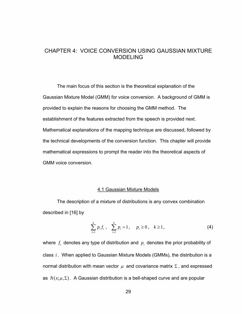
statistical models used for data processing. Basically, GMMs are used by mixing

Gaussian distributions with varying means and variances to produce a unique

contour with varying peaks. GMM can be used to cluster the spectral distribution

for voice conversion. Each cluster will contain its own centroid, or mean. The

spread of the cluster is considered the variance. Therefore, each cluster exhibits

the qualities of a Gaussian distribution with a centroid μ and a spread Σ . Figure

12 shows how data points are classified by GMM.

Figure 12: The clustering of data points using GMM with prior probabilities.

31

The figure provides much insight in GMM. The number of clusters refer

the number of mixtures, often denoted by Q . The number of mixtures can only

be determined by the user, and not by the algorithm. As one can deduce, the

more mixtures involved, the more precise the classification, resulting in

minimization of errors.

4.2 Choosing GMM for Conversion

As discussed in [17], the GMM method was shown to be more efficient

and robust than previously known techniques based on vector quantization (VQ).

This is first shown in the comparison of relative spectral distortion of both

methods shown in Figure 13. Relative spectral distortion refers to the average

quadratic spectral distortion of the mean squared error normalized by the initial

distortion between both source and target speaker.

32

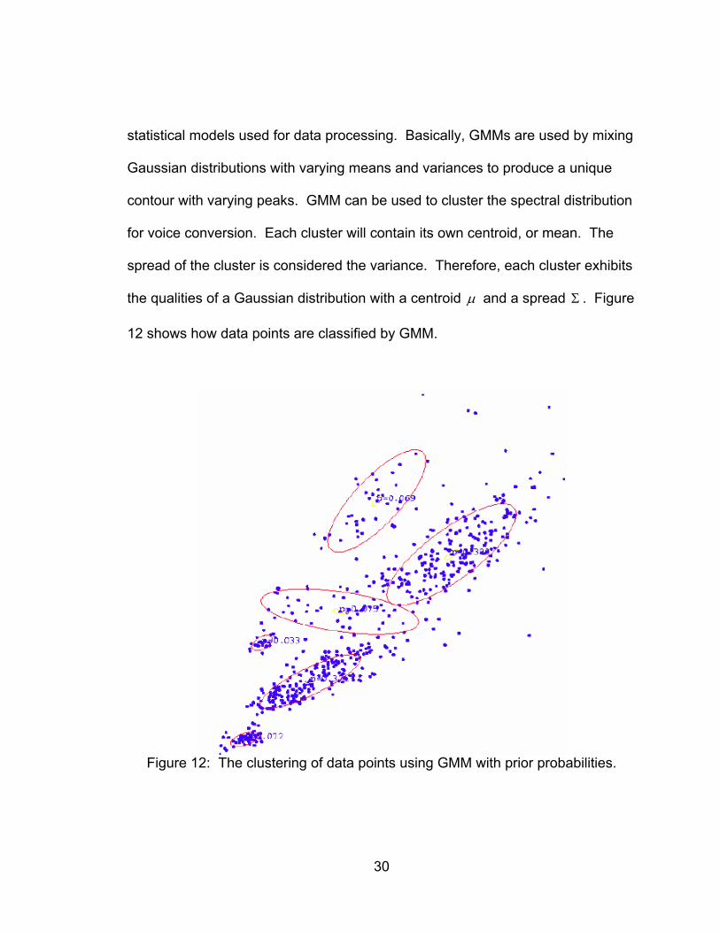
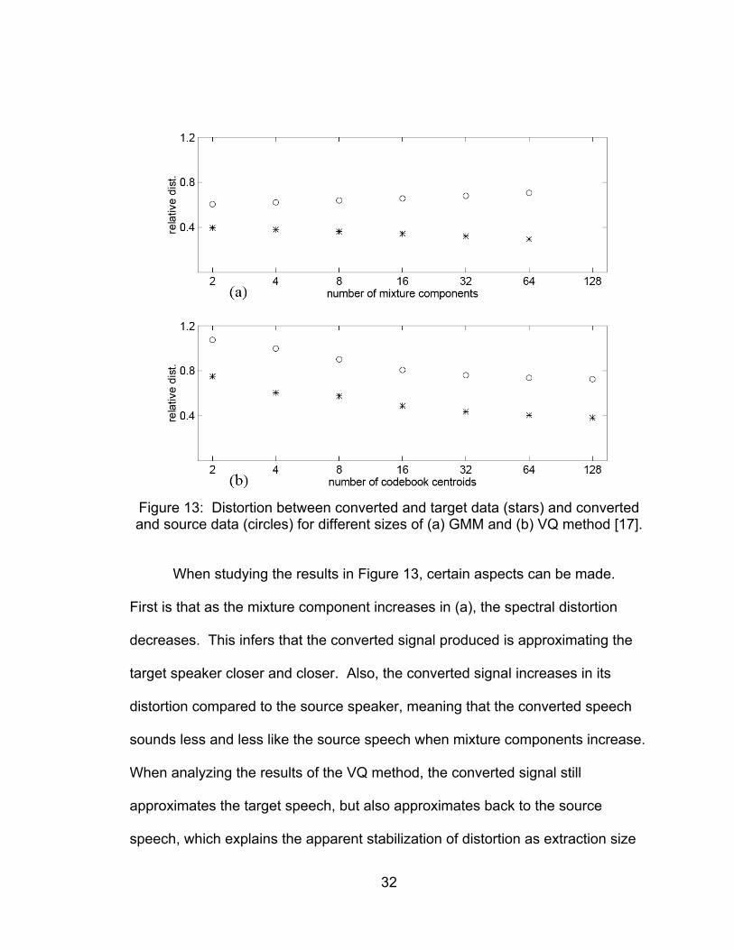
Figure 13: Distortion between converted and target data (stars) and converted and source data (circles) for different sizes of (a) GMM and (b) VQ method [17].

When studying the results in Figure 13, certain aspects can be made.

First is that as the mixture component increases in (a), the spectral distortion

decreases. This infers that the converted signal produced is approximating the

target speaker closer and closer. Also, the converted signal increases in its

distortion compared to the source speaker, meaning that the converted speech

sounds less and less like the source speech when mixture components increase.

When analyzing the results of the VQ method, the converted signal still

approximates the target speech, but also approximates back to the source

speech, which explains the apparent stabilization of distortion as extraction size

33

increases. Also inferred from the results are that distortion values are much

greater in the case of the VQ method where a codebook size of 512 vectors

produced a distortion 17% higher than using a mixture component of 64 for the

GMM method.

The advantages of using the GMM method include soft clustering and

continuous transform. Soft clustering refers to the characteristics of the mixture

of Gaussian densities. The mixture model allows for “smooth” transitions of the

spectral parameters’ classifications. This characteristic avoids the unnatural

discontinuities in the VQ method caused by the vector jumps of classes,

providing improved synthesis quality. The characteristic of a continuous

transform reduces the unwanted spectral distortions observed by the VQ method

because the GMM method considers each class a cluster instead of a single

vector. No further studies of VQ methods have resolved the problems of

discontinuities in using the VQ version as well as the GMM version does.

Additionally, the amount of assistance of the GMM method helped to

determine the selection as well. Since not as many studies were able to be

found referring to other various methods of voice conversion, the choices for the

thesis selection was limited. Studies of [5], [6], [7], and [18] provided greater

learning materials for voice conversion than those found for other methods.

34

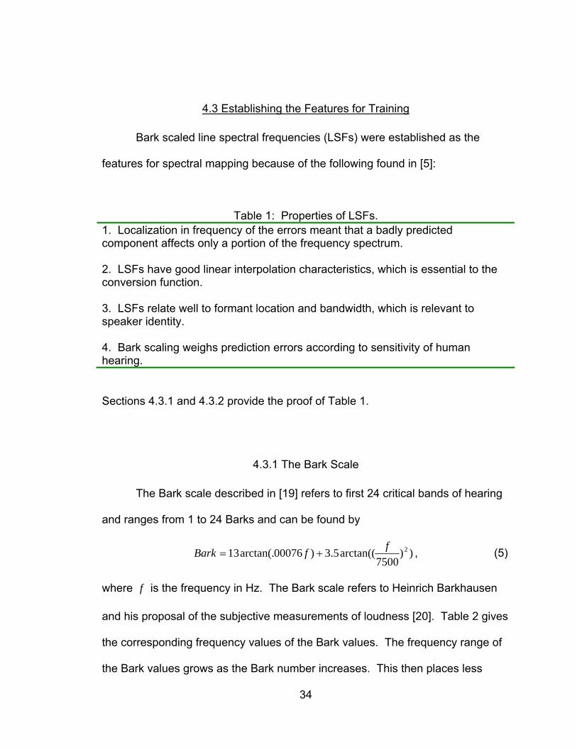
4.3 Establishing the Features for Training

Bark scaled line spectral frequencies (LSFs) were established as the

features for spectral mapping because of the following found in [5]:

Table 1: Properties of LSFs. 1. Localization in frequency of the errors meant that a badly predicted component affects only a portion of the frequency spectrum. 2. LSFs have good linear interpolation characteristics, which is essential to the conversion function. 3. LSFs relate well to formant location and bandwidth, which is relevant to speaker identity. 4. Bark scaling weighs prediction errors according to sensitivity of human hearing.

Sections 4.3.1 and 4.3.2 provide the proof of Table 1.

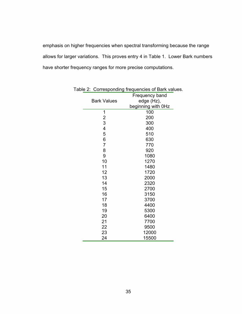
4.3.1 The Bark Scale

The Bark scale described in [19] refers to first 24 critical bands of hearing

and ranges from 1 to 24 Barks and can be found by

))7500

arctan((5.3)00076arctan(.13 2ffBark += , (5)

where f is the frequency in Hz. The Bark scale refers to Heinrich Barkhausen

and his proposal of the subjective measurements of loudness [20]. Table 2 gives

the corresponding frequency values of the Bark values. The frequency range of

the Bark values grows as the Bark number increases. This then places less

35

emphasis on higher frequencies when spectral transforming because the range

allows for larger variations. This proves entry 4 in Table 1. Lower Bark numbers

have shorter frequency ranges for more precise computations.

Table 2: Corresponding frequencies of Bark values.

Bark Values Frequency band

edge (Hz), beginning with 0Hz

1 100 2 200 3 300 4 400 5 510 6 630 7 770 8 920 9 1080 10 1270 11 1480 12 1720 13 2000 14 2320 15 2700 16 3150 17 3700 18 4400 19 5300 20 6400 21 7700 22 9500 23 12000 24 15500

36

In order to convert to a Bark scale, the LPC process is used to estimate

the vocal tract filter )(

1zA

. In [21], an all pass warped bilinear transform is used

to only affect the phase of the vocal tract filter with the mapping of

111

1~)( −−

−

−

↔=−−

= zzz

zzBa λλ . (6)

Equation 6 implies that each unit delay is substituted with the warped bilinear

1~ −z , effectively transforming the z -domain into the modified z~ -domain. While

aB is 1, the phase is calculated to be

.)cos(1

)sin(arctan2~⎟⎟⎠

⎞⎜⎜⎝

⎛−

+=ωλ

ωλωω (7)

The warping factor λ is found to be .76 for Bark scaling in [19]. Therefore if the

LSFs using the original z -domain were calculated from the spectrum, then

Equation 7 will convert the z -domain LSFs to the Bark scaled LSFs.

4.3.2 LSF Computation

Remember that the LPC technique requires )(zA to be in the form of

MM

M

m

mmM zfzfzfzF −−

=

− −−−=−= ∑ L11

011)( . (8)

In order for the filter )(

1zA

characterized by the vocal tract to be stable, the poles

must be inside the unit circle in the z -domain [22]. Therefore, the zeros of )(zA

must lie inside the z -domain unit circle. The goal of LSFs is to find a

37

representation of the zeros that lie on the unit circle. This is first done by finding

the corresponding palindromic and antipalindromic equivalent of Equation 8

noted by )(zP and )(zQ respectively.

In [23], a polynomial with degree M can be defined as “palindromic” when

mMm ff −= , (9)

and “antipalindromic” if

mMm ff −−= . (10)

Properties of these types of polynomials include that the product of two

palindromic or antipalindromic polynomials is palindromic. The product of a

palindromic and antipalindromic polynomial gives an antipalindromic polynomial.

The next step is to prove that polynomials with zeros on the unit circle are

either palindromic or antipalindromic. It is easy to see that 1+x and 1−x are

palindromic and antipalindromic respectively. Now consider a second order

polynomial with complex conjugate zeros on the unit circle,

.)cos(21

1)1)(1()(

21

211

11

−−

−−−−−

−−−

+−=

+−−=

−−=

zzzeezeze

zezezTiiii

ii

φ

φφφφ

φφ

(11)

Equation 11 is palindromic because of the condition in (9), and due to the

properties of palindromics, any polynomial that has k complex conjugate pairs

on the unit circle will be the product of k palindromic polynomials, resulting in a

palindromic polynomial. Further, when (11) is multiplied by 1+x or 1−x , the

result is a palindromic or antipalindromic polynomial respectively.

38

Now that )(zP and )(zQ have been proven to contain zeros lying on the

unit circle, Equation 8 for )(zA can be written as the sum of a palindromic )(zP

and antipalindromic )(zQ [24]. That is

))()((21)( zQzPzAM += , (12)

where

)()()( 1)1( −+−+= zAzzAzP MM

M (13)

and

)()()( 1)1( −+−−= zAzzAzQ MM

M . (14)

Notice that )(zP and )(zQ are of the order 1+M , and follow (9) and (10)

respectively.

From [25], combining (13) and (14) by the factorization of Equation 11

yields a set of equations such that

∏−=

−−− +−+=1,,3,1

211 )cos21()1()(Mi

i zzzzPL

θ (15)

and

∏=

−−− +−−=Mi

i zzzzQ,,4,2

211 )cos21()1()(L

θ , (16)

whenever M is even, and

∏=

−− +−=Mi

i zzzP,,3,1

21 )cos21()(L

θ (17)

and

∏−=

−−−− +−+−=1,,4,2

2111 )cos21()1)(1()(Mi

i zzzzzQL

θ , (18)

39

for the case when M is odd.

Solving for the iθ s using Equation 8 yields the values used for the LSFs,

and follows from (17) and (18) that

πθθθθ <<<<<< − MM 1210 L . (19)

Notice that the values alternate between the )(zP and )(zQ zeros.

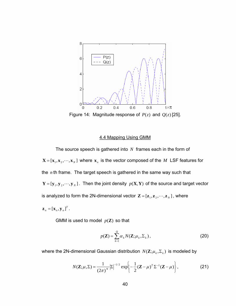
Figure 14 shows the magnitude response of a typical )(zP and )(zQ

solution set for 12=M . Since the vocal tract filter )(

1zA

can be expressed by

Equation 12, any badly predicted component is localized in frequency thereby

proving entry 1 in Table 1. Also due to Equation 12, it has been experimentally

found in [1] that 2

21 θθ + is a good frequency indicator of formants, thus proving

entry 3 in Table 1. Finally, entry 2 from Table 1 can be proven because LSFs

represent the same physical interpretation, which can be further explained in

[26].

40

Figure 14: Magnitude response of )(zP and )(zQ [25].

4.4 Mapping Using GMM

The source speech is gathered into N frames each in the form of

],,,[ 21 NxxxX L= where nx is the vector composed of the M LSF features for

the n th frame. The target speech is gathered in the same way such that

],,,[ 21 NyyyY L= . Then the joint density ),( YXp of the source and target vector

is analyzed to form the 2N-dimensional vector ],,,[ 21 NzzzZ L= , where

Tnnn ],[ yxz = .

GMM is used to model )(Zp so that

∑=

Σ=Q

kkkk Np

1

),;()( μα ZZ , (20)

where the 2N-dimensional Gaussian distribution ),;( kkN ΣμZ is modeled by

⎭⎬⎫

⎩⎨⎧ −Σ−−Σ=Σ −− )()(

21exp

)2(1),;( 12/1 μμπ

μ ZZZ TNN , (21)

41

with ⎥⎦

⎤⎢⎣

⎡= Y

X

k

kk μ

μμ and ⎥

⎦

⎤⎢⎣

⎡

ΣΣΣΣ

=Σ YYYX

XYXX

kk

kkk .

The parameters ),,( Σμα can be obtained by the Expectation

Maximization (EM) algorithm [27]. The EM algorithm first initiates values for the

parameters. Then the following formulas

∑=

=N

nnkk Cp

N 1

)|(1* zα (22)

∑∑

=

== N

n nk

nN

n nkk

Cp

Cp

1

1

)|(

)|(*

z

zzμ (23)

2

1

12

*)|(

)|(* kN

n nk

N

n nnkk

Cp

zCpμ−=Σ

∑∑

=

=

z

z (24)

where 2nz refers to an arbitrary element of nz and

∑ =

Σ

Σ= Q

j jjnj

kknknk

NN

Cp1

),;(),;(

)|(μα

μα

zz

z (25)

can be used to estimate the maximum likelihood of the parameters ),,( Σμα .

Equations 22, 23, and 24 are the newly estimated parameters calculated from

the old parameters through Equation 25. Equation 25 also describes the

conditional probability that a given vector nz belongs to class kC and is derived

from the application of Bayes’ rule [28].

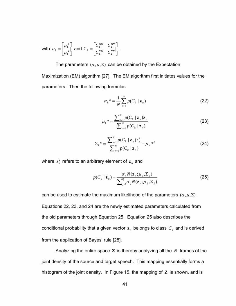
Analyzing the entire space Z is thereby analyzing all the N frames of the

joint density of the source and target speech. This mapping essentially forms a

histogram of the joint density. In Figure 15, the mapping of Z is shown, and is

42

read very much like a topographical map. The horizontal axis indicates the

M features of the source, while the vertical axis indicates those of the target

speaker. All the data from all frames is depicted in the figure. The various colors

on the plot is used to label the class of the data point. Then, the class forms the

generated Gaussian distribution. The final forms a 3d mixture Gaussian curve

for the distribution of )(Zp and visually similar to that of a mountain range with

various peaks and valleys.

Figure 15: The mapping of the joint speaker acoustic space through GMM [29].

4.5 Developing the Conversion Function for Vocal Tract Conversion

The goal of the conversion function is to minimize the mean squared error

]))([( 2XY FEmse −=ε , (26)

where E is expectation. If )(XF is assumed to be a non-linear function, then

Equation 26 can be solved using conditional expectation [30] such that

43

.)(]|))([(

]]|))([([]))([(2

22

∫∞

∞−=−=

−=−

dxxfFE

gEEFE

XxXXY

XXYXY (27)

Since the term inside the integral in (27) is always positive, then the problem is

simply a matter of minimizing that term. The result is that the function that

minimizes the mean squared error is the conditional expectation, and is often

called the regression curve. Therefore the regression curve for the joint

Gaussian case will be

]|[)( XYX EF = . (28)

To find this, it is known that

),;(

),;,(),;|( ||XXX

YXYXXYXY

XXYXY

ΣΣ

=Σμμμ

NNN , (29)

resolving into the following expression for the conditional Gaussian distribution

( )

)1(2

)1(21exp

),;|(2

,

2,

YXYY

YXXX

YX

YYYX

XYXY

ρπ

μμρ

μ−Σ

⎪⎭

⎪⎬⎫

⎪⎩

⎪⎨⎧

⎥⎦

⎤⎢⎣

⎡−−

ΣΣ

−Σ−

−

=ΣN , (30)

and

YYYY

YX

YXΣΣ

Σ=,ρ . (31)

From Equation 30 the expected value for the conditional distribution is found to

be linear and of the form

( ) YXXX

YX

XXY μμ +−ΣΣ

=]|[E . (32)

44

The result of Equation 32 is applied to Gaussian mixtures by the weighting term

of the probability the vector nx belongs to a class kC . The final conversion

function is developed into

( ) ⎥⎦

⎤⎢⎣

⎡+−

ΣΣ

= ∑=

YXXX

YX

XXX kkk

kQ

kkCpF μμ)|()(

1

, (33)

where

∑ =

Σ

Σ= Q

j jjj

kkkk

NN

Cp1

),;(),;(

)|(XXX

XXX

XX

Xμα

μα. (34)

4.6 Converting the Fundamental Frequency F0

Recall the Source Filter model for speech is composed of the excitation

signal )(nε and the vocal tract filter )(/1 zA . In order to execute a successful

conversion, both of these components are converted to resemble the target

speaker. The vocal tract filter parameters were converted as discussed in

Section 4.5. The excitation is now the only parameter that must be converted

before obtaining the final converted speech. To do this, the source speaker’s

fundamental frequency (F0) is scaled to match on average the target speaker’s

F0. The following expression,

tts

ss

t ff μσ

σμ

+−

= 00 , (35)

was used to convert to the source F0 to the projected target F0 [31]. The mean

and standard deviations were calculated on all the F0 from the voiced frames in

45

the speech. The F0 can be found using a variety of techniques such as the

autocorrelation method and the cepstrum method.

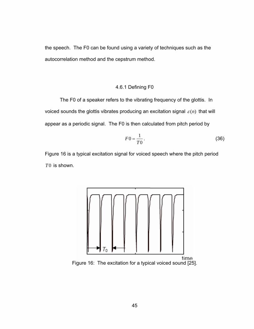
4.6.1 Defining F0

The F0 of a speaker refers to the vibrating frequency of the glottis. In

voiced sounds the glottis vibrates producing an excitation signal )(nε that will

appear as a periodic signal. The F0 is then calculated from pitch period by

0

10T

F = . (36)

Figure 16 is a typical excitation signal for voiced speech where the pitch period

0T is shown.

Figure 16: The excitation for a typical voiced sound [25].

46

The excitation signal for an unvoiced sound appears as noise with no

periodic characteristics. Since there is no period for unvoiced sounds, it has no

F0. Figure 17 shows the signal )(nε for an unvoiced sound.

Figure 17: The excitation for a typical unvoiced sound [25].

The F0 varies from person to person. In females, F0 ranges from 120 to 500 Hz,

while the range varies from 50 to 250 Hz in men [32].

4.6.2 Extracting F0

The Autocorrelation method is a popular technique for finding the F0 in

voiced segments. If the F0 is to be estimated from )(ns and the frame that ends

at time instant m with a frame length of T , then the autocorrelation is defined by

∑+−=

−=m

Tmn

nsnsR1

)()()( ττ , (37)

where τ is the time lag in samples [32]. Equation 36 reflects the similarity

between the frame that starts at time instant 1+−= Tmn to m to the time shifted

version. The value for τ that yields the largest value of the autocorrelation is

determined to be the pitch period. Figure 18 and Figure 19 show the speech

waveform of a voiced sound with the autocorrelation respectively, where the

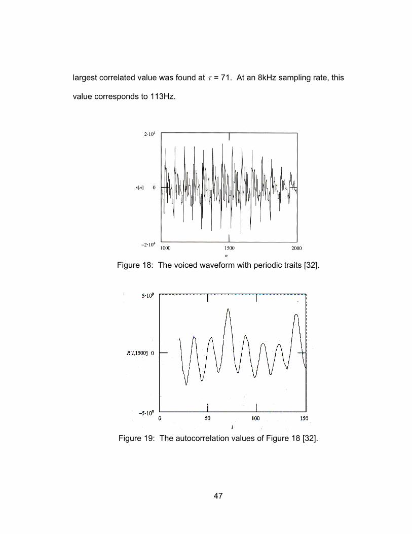
47

largest correlated value was found at τ = 71. At an 8kHz sampling rate, this

value corresponds to 113Hz.

Figure 18: The voiced waveform with periodic traits [32].

Figure 19: The autocorrelation values of Figure 18 [32].

48

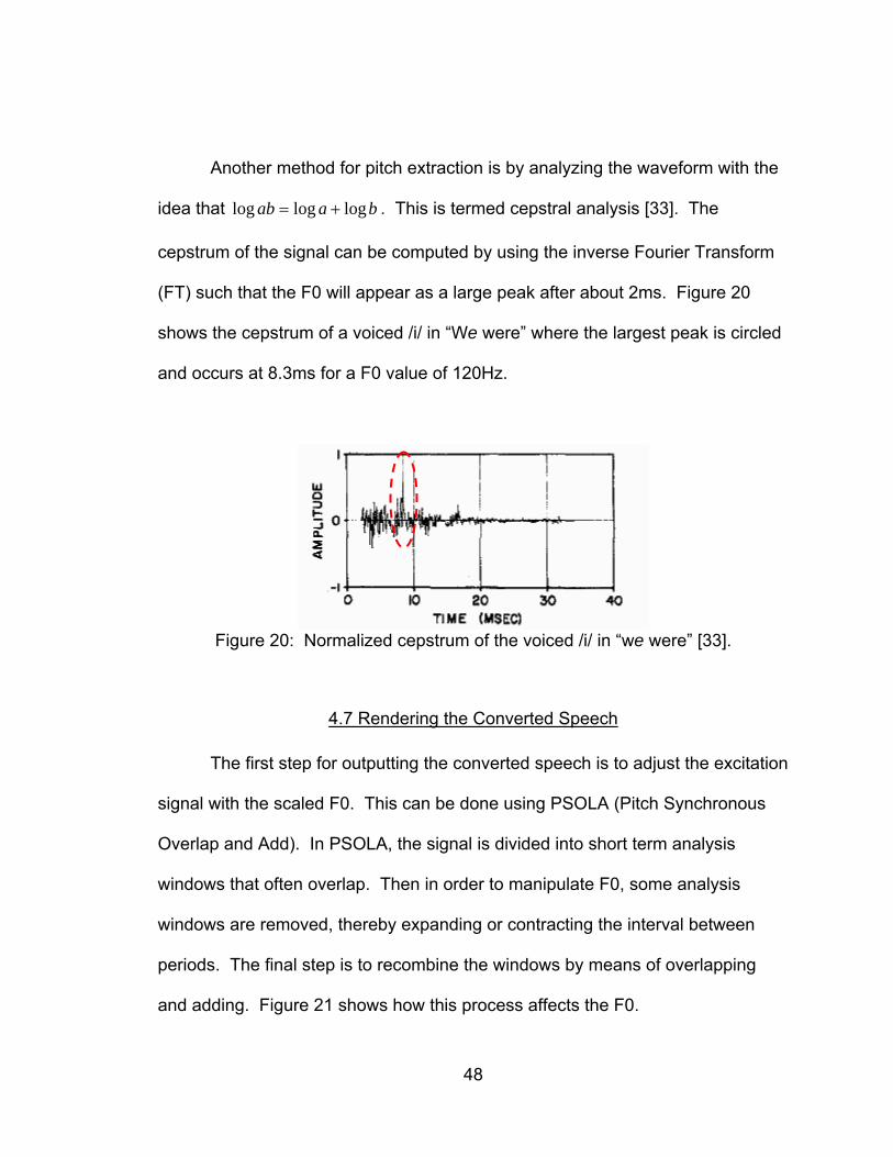
Another method for pitch extraction is by analyzing the waveform with the

idea that baab logloglog += . This is termed cepstral analysis [33]. The

cepstrum of the signal can be computed by using the inverse Fourier Transform

(FT) such that the F0 will appear as a large peak after about 2ms. Figure 20

shows the cepstrum of a voiced /i/ in “We were” where the largest peak is circled

and occurs at 8.3ms for a F0 value of 120Hz.

Figure 20: Normalized cepstrum of the voiced /i/ in “we were” [33].

4.7 Rendering the Converted Speech

The first step for outputting the converted speech is to adjust the excitation

signal with the scaled F0. This can be done using PSOLA (Pitch Synchronous

Overlap and Add). In PSOLA, the signal is divided into short term analysis

windows that often overlap. Then in order to manipulate F0, some analysis

windows are removed, thereby expanding or contracting the interval between

periods. The final step is to recombine the windows by means of overlapping

and adding. Figure 21 shows how this process affects the F0.

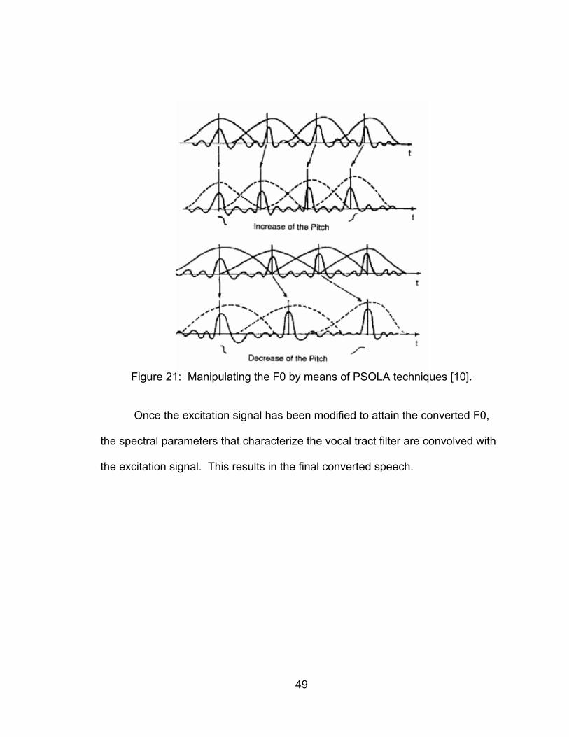
49

Figure 21: Manipulating the F0 by means of PSOLA techniques [10].

Once the excitation signal has been modified to attain the converted F0,

the spectral parameters that characterize the vocal tract filter are convolved with

the excitation signal. This results in the final converted speech.

50

CHAPTER 5: EVALUATIONS

In this Chapter, the various methods for evaluating the different voice

conversion systems in current production is discussed. There are many ways

that these types of tests can be carried out. These methods are mostly broken

down into subjective tests and objective tests. Subjective tests are evaluated by

people listening to various sound files to determine the effectiveness of the voice

converter. Some examples of subjective tests are the ABX test and mean

opinion score (MOS) tests. Since these tests rely on opinions, other means for

testing must be experimented in order to eliminate any biased effects. Therefore

objective tests are also staged to provide additional evaluations. Objective

results are mathematical measures for interpretation of the converted speech.

Typical examples of objective tests include error tests and spectral distortion

measures. The following results are obtained from various types of voice

converters.

5.1 Subjective Measures of Voice Conversion Processes

The subjective measures for various voice conversion methods are

provided to help develop a better understanding of the need for increased

studies. Listening tests can be executed through a variety of experimental

conditions. ABX tests are a common method for listening tests. The main

51

response of this question is “is X closer to A or B?” where A and B are treated as

a control and variable respectively and X is used to measure the closeness to A

or B.

Other common measures are mean opinion scores or MOS. In MOS

experiments, the subject is told to give their opinion on the condition based on a

numeric scale, usually from one to five. The subject must be given an example

of a specific opinion in order to execute these tests. Then the average of the

responses is taken to indicate the success (or failure) of the experiment.

5.1.1 Vector Quantization Results

Recall the description of the VQ method in Section 2.2.1 based on [8].

The training size was 100 words. The codebook size for the spectrum

parameters was 256, with a 12th order LPC analysis. The two experiments that

will be mentioned evaluate the male to female and male to male conversion

performance. The first experiment helps to examine the contribution of the pitch

and spectral parameters to speech individuality through a pair comparing test.

Two different words were used as speech pairs for five different conversions

resulting in a possible combination of 40 tests. Twelve subjects were given the

tests in a soundproof room. The subjects were asked to rate the similarity of

each pair of words according to “similar,” “slightly similar,” “difficult to decide,”

“slightly dissimilar,” and “dissimilar.” Table 3 gives the descriptions of the five

experimental conditions.

52

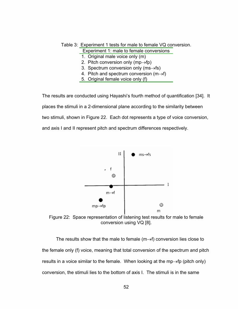
Table 3: Experiment 1 tests for male to female VQ conversion. Experiment 1: male to female conversions 1. Original male voice only (m) 2. Pitch conversion only (mp→fp) 3. Spectrum conversion only (ms→fs) 4. Pitch and spectrum conversion (m→f) 5. Original female voice only (f)

The results are conducted using Hayashi’s fourth method of quantification [34]. It

places the stimuli in a 2-dimensional plane according to the similarity between

two stimuli, shown in Figure 22. Each dot represents a type of voice conversion,

and axis I and II represent pitch and spectrum differences respectively.

Figure 22: Space representation of listening test results for male to female

conversion using VQ [8].

The results show that the male to female (m→f) conversion lies close to

the female only (f) voice, meaning that total conversion of the spectrum and pitch

results in a voice similar to the female. When looking at the mp→fp (pitch only)

conversion, the stimuli lies to the bottom of axis I. The stimuli is in the same

53

bottom half as the male only voice meaning that pitch only conversion is not

efficient for voice conversion. The same can be said about the spectrum only

(ms→fs) conversion. Therefore, it is favorable to convert both the spectrum and

pitch.

The second experiment is of the ABX form with the each ABX question

designed to evaluate the conversion between two male speakers. Four words

were included with each ABX question being comprised of three different words

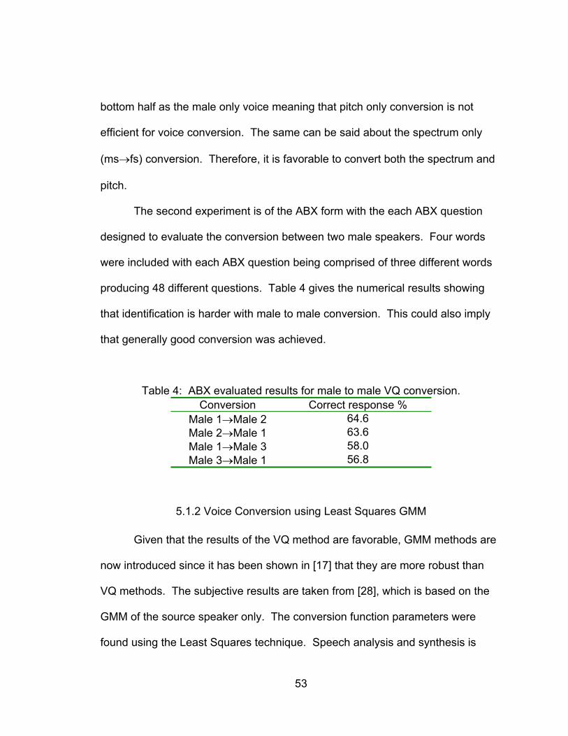
producing 48 different questions. Table 4 gives the numerical results showing

that identification is harder with male to male conversion. This could also imply

that generally good conversion was achieved.

Table 4: ABX evaluated results for male to male VQ conversion. Conversion Correct response %

Male 1→Male 2 64.6 Male 2→Male 1 63.6 Male 1→Male 3 58.0 Male 3→Male 1 56.8

5.1.2 Voice Conversion using Least Squares GMM

Given that the results of the VQ method are favorable, GMM methods are

now introduced since it has been shown in [17] that they are more robust than

VQ methods. The subjective results are taken from [28], which is based on the

GMM of the source speaker only. The conversion function parameters were

found using the Least Squares technique. Speech analysis and synthesis is

54

performed using the Harmonic plus Noise Model (HNM) where the speech signal

is the effect of composing the sum of a purely harmonic signal and of a

modulated noise [35].

The conversion function is applied to the spectral envelopes of the

harmonic aspects of the signal because the noise part was found to be less

stringent to the individuality of the speaker. Overall, the process converts the

harmonics (voiced frames) using the conversion function, and the noise

(unvoiced frames) by a corrective filter that models the difference between the

average noise spectra between the target and source.

The features extracted from the voiced frames used for conversion were

computed from the amplitudes of the harmonics by the discrete regularized

cepstrum method based on a warped frequency scale. The feature order used

for extraction from the voiced frame was 20. Conversion was done between two

male voices provided by the Centre National d’Etudes des Telecommunications

based on phonemes in the French language. About 20,000 training vectors were

used for the training process resulting in 3.5 minutes of voiced speech.

The demonstration of success of the method is performed through two

useful listening tests. The first is the standard ABX test. In this case, X was one

of three types of conversions – pitch only and GMM using mixtures of 16 and 64

with full conversions each. A or B is an uttered sentence by the source or target

speaker consisting of the same words. X is a different sentence uttered, and

subjects were asked to identify whether A or B is closest to X. The pitch only

55

conversion found that only 18% of listeners made a correct identification. The

GMM full conversion method with 16 mixtures provided a dramatically increased

percentage of identification with 83% of correct responses. Increasing the

mixture to 64 yielded a slight increase of 88%. An additional ABX response was

formed where A, B, and X uttered the same sentences and applied to GMM full

conversion with 64 mixtures. In this study, 97% were able to identify the correct

response.

The second study is based on the MOS test, where subjects were asked

to rate the overall performance based on a zero to nine scale with zero meaning

“identical” and nine meaning “very different.” Pairs of speech utterances were

used along with all combinations of original speaker, target speaker, “pitch

modified” speaker, and converted speaker using 16 and 64 GMM mixtures. Each

speech pair uttered a different sentence. Subjects listened to the pair of speech

utterance based on a type of conversion. They were asked to rate the similarity

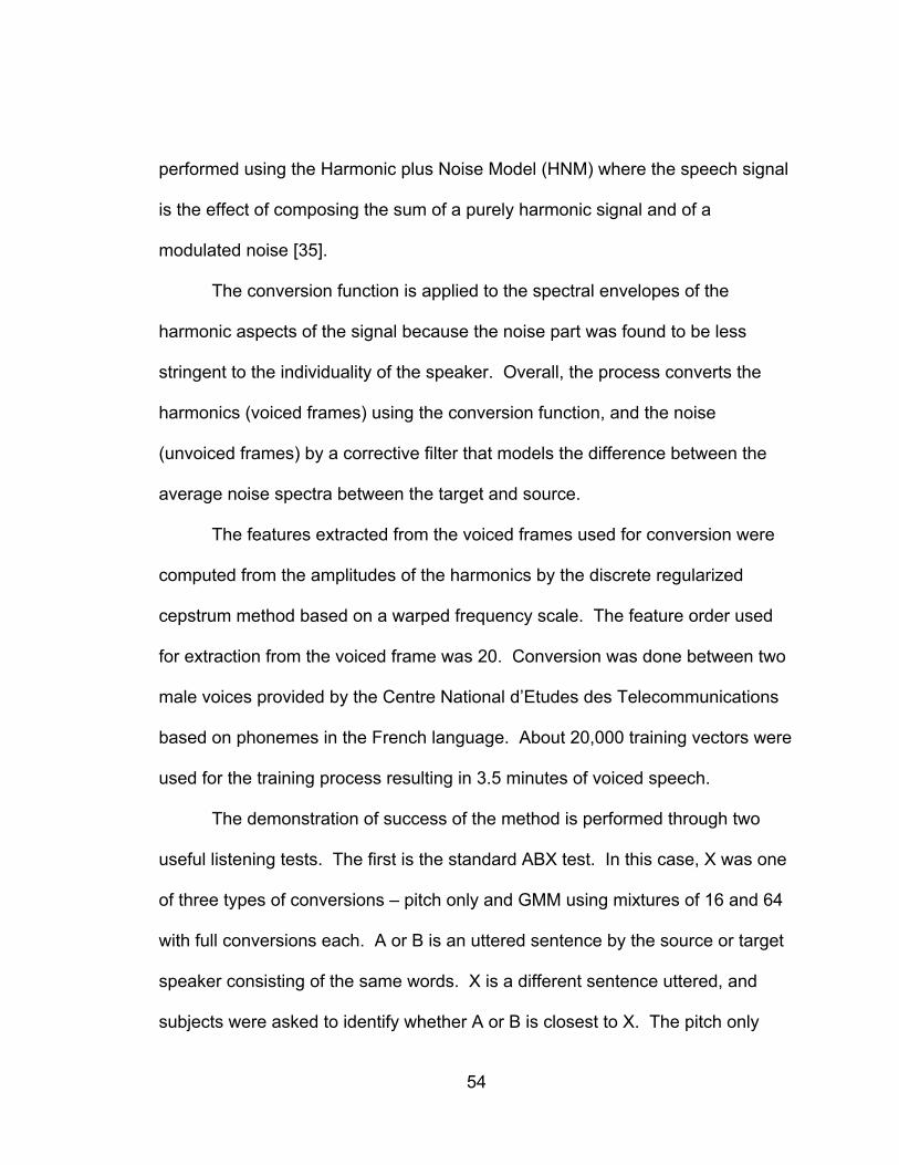
of what they heard. Figure 23 shows the results of the opinion test.

56

Figure 23: Opinion test results of source speaker GMM with the Least Squares

technique [28].

Each type of conversion is labeled as “TT” for target to target, “SS,”

source to source, “M2,” conversion of source using 64 GMM to target, “M1,”

conversion of source using 16 GMM to target, “PT,” source pitch conversion to

target, and “ST” for the source to target. To understand this, imagine one

sentence spoken by the source. In a “SS” question, a different second sentence

is uttered again by the source. Answers given by the subjects should be

relatively close to 0. The “x” in the plot refers to the median value with the lines

referring to the mean absolute deviation of the responses for the type of

combination.

The figure shows that the pitch only method lies relatively close with the

source to target combination. Since “ST” refers to one sentence being uttered by

57

the source, and the other sentence being spoken by the target, responses should

be in the 9 range. This again shows that only changing the pitch is not sufficient

enough for conversion. Using GMM conversion helps the source sound more

like the target speaker. As in agreement with the results of the ABX test, with 64

GMM allowing for a more similar sounding result than 16 GMM.

5.1.3 Results of GMM Conversion of Joint Space

This method of voice conversion is done in [6], and is an expansion of [28]

where instead of modeling only the source speaker distribution using GMM, the

joint of the source and target is used. The theory is that the joint density should

lead to a more judicious allocation of mixtures for the regression.

In [8], two male and a female speaker were selected from the Oregon

Graduate Institute diphone database [36]. The training sets were constructed by

performing a binary split VQ on all vectors of the source speaker database. The

vectors are composed of 16th ordered Bark scaled LSFs extracted from the

frames of each diphone. Diphones whose vectors were closest to one or more

codewords of the VQ procedure were included in the training set. Training set All

consists of all the possible diphones in the database. A GMM distribution with 1,

2, 4, 8, and 16 mixtures was performed for each training set. The conversion

consisted of the spectral vectors followed by pitch modification. For subjective

tests, the mixture that gave the lowest error was used. Table 5 contains the

conditions for the three sets used for evaluations.

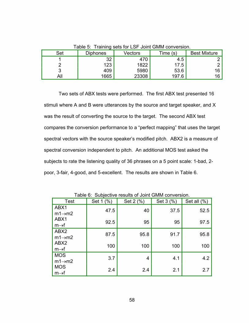
58

Table 5: Training sets for LSF Joint GMM conversion. Set Diphones Vectors Time (s) Best Mixture 1 32 470 4.5 22 123 1822 17.5 23 409 5980 53.6 16All 1665 23308 197.6 16

Two sets of ABX tests were performed. The first ABX test presented 16

stimuli where A and B were utterances by the source and target speaker, and X

was the result of converting the source to the target. The second ABX test

compares the conversion performance to a “perfect mapping” that uses the target

spectral vectors with the source speaker’s modified pitch. ABX2 is a measure of

spectral conversion independent to pitch. An additional MOS test asked the

subjects to rate the listening quality of 36 phrases on a 5 point scale: 1-bad, 2-

poor, 3-fair, 4-good, and 5-excellent. The results are shown in Table 6.

Table 6: Subjective results of Joint GMM conversion. Test Set 1 (%) Set 2 (%) Set 3 (%) Set all (%)

ABX1 m1→m2 47.5 40 37.5 52.5

ABX1 m→f 92.5 95 95 97.5

ABX2 m1→m2 87.5 95.8 91.7 95.8

ABX2 m→f 100 100 100 100

MOS m1→m2 3.7 4 4.1 4.2

MOS m→f 2.4 2.4 2.1 2.7

59

Interpreting the results, ABX1 for male to male conversion shows

comparable findings to Table 4. In fact, the researchers found that some

subjects felt there had been a third male speaker involved. However, the

listening quality for male to male conversion was favorable averaging above

“good.” The male to female conversion resulted in more correct responses which

shows the important role of pitch, but leads to a poorer listening quality compared

to male to male conversion. The average of listening quality in male to female

conversion is slightly below “fair.

In the second ABX test, subjects related the converted speech to the

“perfectly mapped” voice, which consists of the modified source pitch and the

original target spectral envelope, and showed that a strong spectral relationship

was formed. This means that when the residual is ignored, the spectral

conversion is quite successful. Therefore more research must be done in pitch

modification techniques (refer to Section 5.2.5).

5.2 Objective Measure of Voice Conversion Processes

Objective measures quantify the performance of the voice conversion.

Typical measures are based on relative spectral distortions. Relative spectral

distortion compares the distance between converted speech and the reference,

with that between source and reference [37]. Spectral distortions themselves

vary according to the differences in distances. Therefore in objective measures,

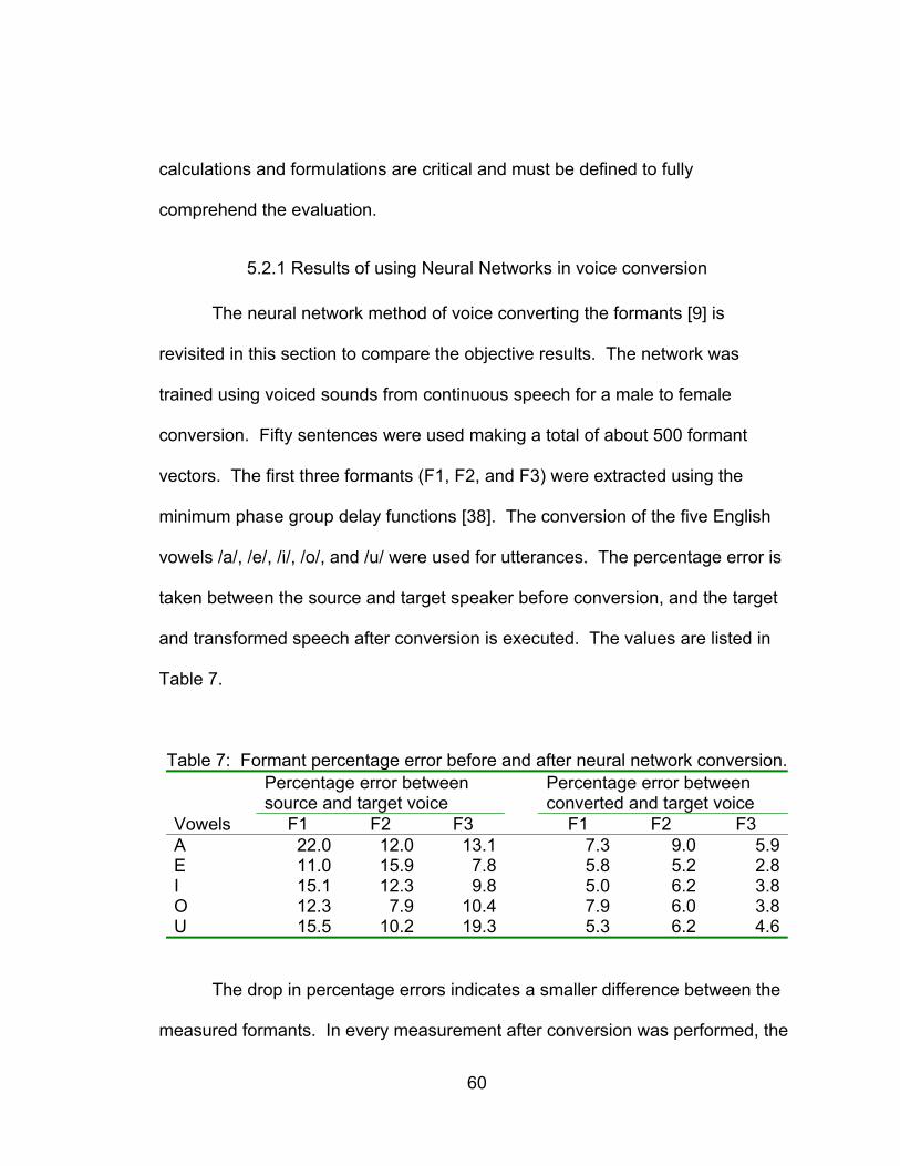
60

calculations and formulations are critical and must be defined to fully

comprehend the evaluation.

5.2.1 Results of using Neural Networks in voice conversion

The neural network method of voice converting the formants [9] is

revisited in this section to compare the objective results. The network was

trained using voiced sounds from continuous speech for a male to female

conversion. Fifty sentences were used making a total of about 500 formant

vectors. The first three formants (F1, F2, and F3) were extracted using the

minimum phase group delay functions [38]. The conversion of the five English

vowels /a/, /e/, /i/, /o/, and /u/ were used for utterances. The percentage error is

taken between the source and target speaker before conversion, and the target

and transformed speech after conversion is executed. The values are listed in

Table 7.

Table 7: Formant percentage error before and after neural network conversion. Percentage error between

source and target voice Percentage error between

converted and target voice Vowels F1 F2 F3 F1 F2 F3 A 22.0 12.0 13.1 7.3 9.0 5.9E 11.0 15.9 7.8 5.8 5.2 2.8I 15.1 12.3 9.8 5.0 6.2 3.8O 12.3 7.9 10.4 7.9 6.0 3.8U 15.5 10.2 19.3 5.3 6.2 4.6

The drop in percentage errors indicates a smaller difference between the

measured formants. In every measurement after conversion was performed, the

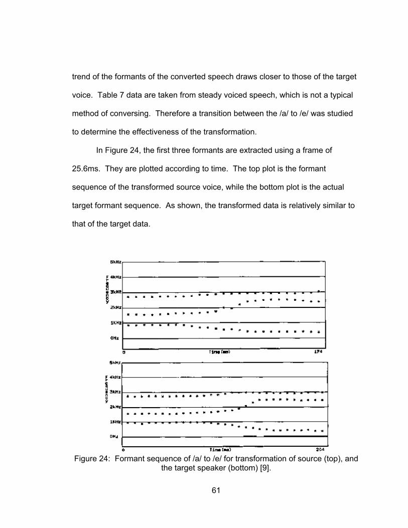
61

trend of the formants of the converted speech draws closer to those of the target

voice. Table 7 data are taken from steady voiced speech, which is not a typical

method of conversing. Therefore a transition between the /a/ to /e/ was studied

to determine the effectiveness of the transformation.

In Figure 24, the first three formants are extracted using a frame of

25.6ms. They are plotted according to time. The top plot is the formant

sequence of the transformed source voice, while the bottom plot is the actual

target formant sequence. As shown, the transformed data is relatively similar to

that of the target data.

Figure 24: Formant sequence of /a/ to /e/ for transformation of source (top), and

the target speaker (bottom) [9].

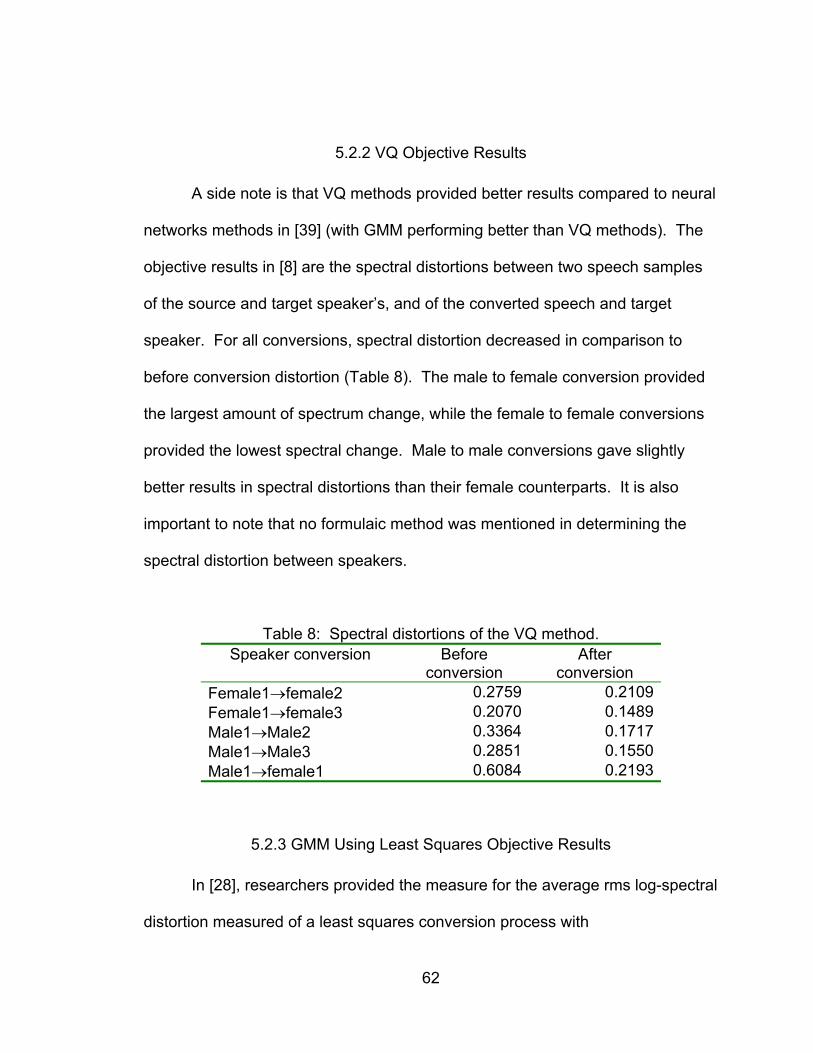
62

5.2.2 VQ Objective Results

A side note is that VQ methods provided better results compared to neural

networks methods in [39] (with GMM performing better than VQ methods). The

objective results in [8] are the spectral distortions between two speech samples

of the source and target speaker’s, and of the converted speech and target

speaker. For all conversions, spectral distortion decreased in comparison to

before conversion distortion (Table 8). The male to female conversion provided

the largest amount of spectrum change, while the female to female conversions

provided the lowest spectral change. Male to male conversions gave slightly

better results in spectral distortions than their female counterparts. It is also

important to note that no formulaic method was mentioned in determining the

spectral distortion between speakers.

Table 8: Spectral distortions of the VQ method. Speaker conversion Before

conversion After

conversion Female1→female2 0.2759 0.2109 Female1→female3 0.2070 0.1489 Male1→Male2 0.3364 0.1717 Male1→Male3 0.2851 0.1550 Male1→female1 0.6084 0.2193

5.2.3 GMM Using Least Squares Objective Results

In [28], researchers provided the measure for the average rms log-spectral

distortion measured of a least squares conversion process with

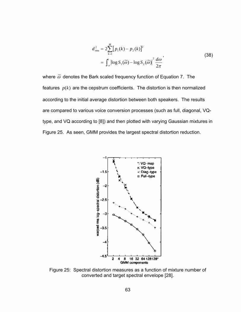
63

[ ]

πωωω

π

π 2)~(log)~(log

)()(2

2

21

1

221

2rms

dSS

kpkpdM

k

∫

∑

−

=

−=

−=, (38)

where ω~ denotes the Bark scaled frequency function of Equation 7. The

features )(kp are the cepstrum coefficients. The distortion is then normalized

according to the initial average distortion between both speakers. The results

are compared to various voice conversion processes (such as full, diagonal, VQ-

type, and VQ according to [8]) and then plotted with varying Gaussian mixtures in

Figure 25. As seen, GMM provides the largest spectral distortion reduction.

Figure 25: Spectral distortion measures as a function of mixture number of

converted and target spectral envelope [28].

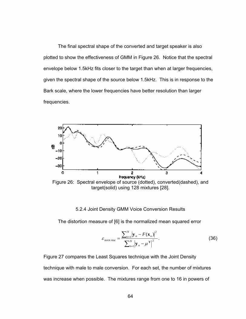
64

The final spectral shape of the converted and target speaker is also

plotted to show the effectiveness of GMM in Figure 26. Notice that the spectral

envelope below 1.5kHz fits closer to the target than when at larger frequencies,

given the spectral shape of the source below 1.5kHz. This is in response to the

Bark scale, where the lower frequencies have better resolution than larger

frequencies.

Figure 26: Spectral envelope of source (dotted), converted(dashed), and

target(solid) using 128 mixtures [28].

5.2.4 Joint Density GMM Voice Conversion Results

The distortion measure of [6] is the normalized mean squared error

∑∑

=

=

−

−=

N

n n

N

n nnmsenorm

F

1

21

2)(Yy

xy

με . (36)

Figure 27 compares the Least Squares technique with the Joint Density

technique with male to male conversion. For each set, the number of mixtures

was increase when possible. The mixtures range from one to 16 in powers of

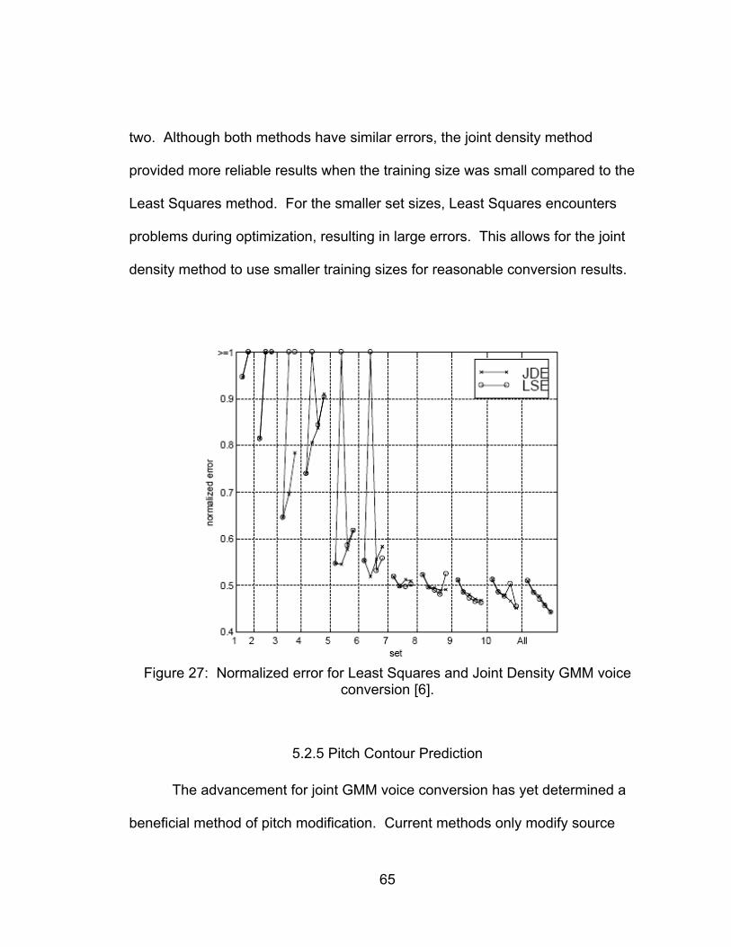
65

two. Although both methods have similar errors, the joint density method

provided more reliable results when the training size was small compared to the

Least Squares method. For the smaller set sizes, Least Squares encounters

problems during optimization, resulting in large errors. This allows for the joint

density method to use smaller training sizes for reasonable conversion results.

Figure 27: Normalized error for Least Squares and Joint Density GMM voice

conversion [6].

5.2.5 Pitch Contour Prediction

The advancement for joint GMM voice conversion has yet determined a

beneficial method of pitch modification. Current methods only modify source

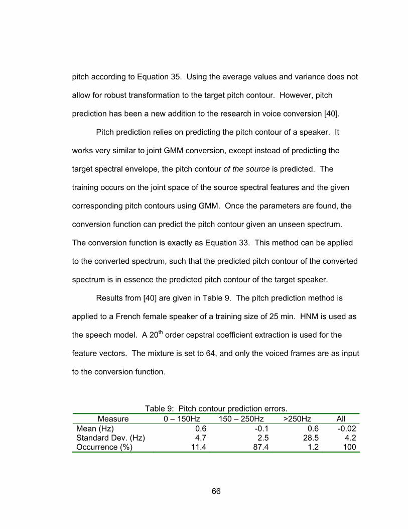
66

pitch according to Equation 35. Using the average values and variance does not

allow for robust transformation to the target pitch contour. However, pitch

prediction has been a new addition to the research in voice conversion [40].

Pitch prediction relies on predicting the pitch contour of a speaker. It

works very similar to joint GMM conversion, except instead of predicting the

target spectral envelope, the pitch contour of the source is predicted. The

training occurs on the joint space of the source spectral features and the given

corresponding pitch contours using GMM. Once the parameters are found, the

conversion function can predict the pitch contour given an unseen spectrum.

The conversion function is exactly as Equation 33. This method can be applied

to the converted spectrum, such that the predicted pitch contour of the converted

spectrum is in essence the predicted pitch contour of the target speaker.

Results from [40] are given in Table 9. The pitch prediction method is

applied to a French female speaker of a training size of 25 min. HNM is used as

the speech model. A 20th order cepstral coefficient extraction is used for the

feature vectors. The mixture is set to 64, and only the voiced frames are as input

to the conversion function.

Table 9: Pitch contour prediction errors. Measure 0 – 150Hz 150 – 250Hz >250Hz All

Mean (Hz) 0.6 -0.1 0.6 -0.02Standard Dev. (Hz) 4.7 2.5 28.5 4.2Occurrence (%) 11.4 87.4 1.2 100

67

CHAPTER 6: DISCUSSIONS

This section provides a brief analysis of the overall effect of using the

discussed techniques for the restoration of voice. Problems encountered and

implementation methods provide further insight into the thesis topic. A section on

future work may also assist in the motivation of expanding current research

projects focused in these similar areas of study.

6.1 Introducing the Method to Solve Current Problems

In order to apply this technique for current use, the overall systems will

depend on several processes. First, the text to speech synthesizer converts the

text into speech. Then the output of the synthesizer is used to provide the

source voice for the voice conversion process. The spectral parameters are

extracted from the conversion process to provide the signal processing for final

speech generation. A typical over all system will look like Figure 28.

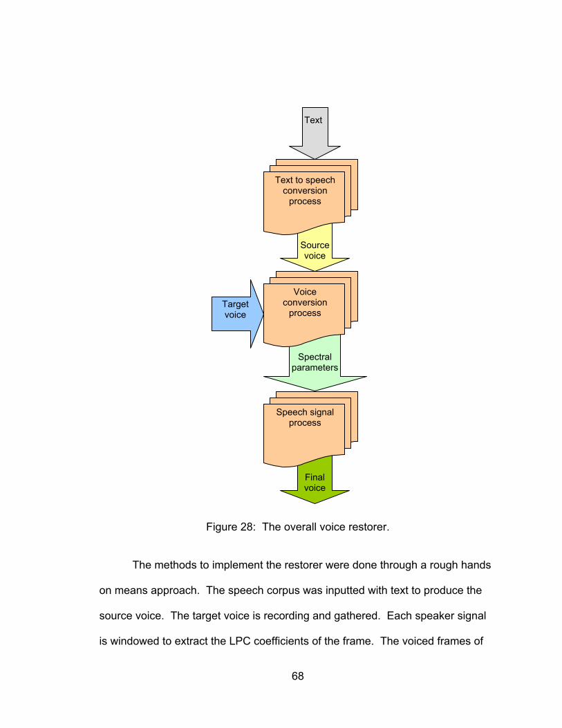
68

Figure 28: The overall voice restorer.

The methods to implement the restorer were done through a rough hands

on means approach. The speech corpus was inputted with text to produce the

source voice. The target voice is recording and gathered. Each speaker signal

is windowed to extract the LPC coefficients of the frame. The voiced frames of

Final voice

Spectral parameters

Source voice

Text to speech conversion

process

Text

Voice conversion

process Target voice

Speech signal process

69

both speakers are specially analyzed for pitch extraction. The LSFs are found

from the LPC, and converted to Bark scale. Features are then aligned by hand

according to phonemes. The EM algorithm is used to estimate the newly formed

joint density space. The conversion function is formed based on the EM

parameters and a linear regression. Then a desired converted sequence is

formed from the TTS system. The source sequence is processed similarly to

training to extract the LSF features. The converted features are found by

inputting the source features into the conversion function. The average and

variance of the pitch is found from the voiced frames, and applied to transform

the pitch of the inputted source sequence. The newly found spectral features

and the modified pitch are convolved to form the converted speech. The

disadvantages of using this type of method are that it is time consuming and

doesn’t really achieve the independent human interaction desired.

Instead it would be more efficient for the system to rely heavily on speech

recognition. By extracting the phonemes of the speech corpus using speech

recognition after synthesis, force alignment programs can also be preformed on

the corpus. This will ensure one to one matching of phonemes for training.

Then, the forced aligned speech corpus could be voice converting, producing the

final converted speech. This method allows for less human dependence besides

the text input required from the speaker.

Dynamic time warping algorithms allows for comparisons to be made

between speech corpora that are not aligned. Algorithms described in [41] can

70

be used to time warp the speech corpora. In order to recognize the speech,

programs such as Carnegie Mellon University’s SPHINX toolkit provided by the

CMU Speech Group (http://www.speech.cs.cmu.edu/sphinx/tutorial.html) can be

used. Both of the software used in conjunction allow for the training process for

voice conversion to begin. The voice conversion process itself cab be utilized in

MATLAB. The final step of using signal processing techniques to obtain the

converted speech still however produces programming challenges.

6.2 Challenges Encountered

Being able to allow independent signal processing for the final voice

output is still a challenge. Current methods require adjustments of the pitch

contour of the source speaker. During this phase of the restorer, the quality of

the voice is degraded. In order to improve the quality of the voice, studies such

as [29], begin by instantiating a speech corpus exclusively designed for voice

conversion.

Another challenge arises in the determination of the quality between

various voice conversion systems. Since voice conversion systems vary by the

methodology used to execute conversion, comparisons across systems are

difficult to conclude. Therefore a comparative assertion must be made in order to

advance the efforts of voice conversion systems. Baseline definitions can be

made in the speech corpus used for training software. Other baseline

71

discriminators can be made in the selection of using the appropriate source voice

for converting.

Potential abuse always surfaces with the advent of new technology. Since

the aim is to mimic the target speaker, identity issues evolve. Speech

recognition software is especially exposed to such abuse with no apparent

solution. However, companies that exploit the use of speech recognition use

verbal passwords to help avert stolen identities. Passwords are the first line

methods for preventing abuse of voice restorers.

6.3 Future work

Aspects of this thesis discussed methods of restoring voice. Voice

conversion techniques are relatively new, and have yet to become commonplace

in society. This allows for time to improve the current proposed systems to

develop a more reliable system. Easy changes such as stronger mapping

models and performing the restoration without human interaction, may help

provide better performance than that attained from the current restoration

process.

The first improvement can be executed during the mapping training

process. During this process, the speech corpora are mapped using Gaussian

mixture modeling. GMM on joint density allowed for a more judicious allocation

of mixtures components. As previously discussed, neural networks and vector

quantization are also realizable mapping methods. Instead of asking which

72

method is more functional, the focus should be when a certain method is more

functional. By asking this question, we can realize a system that uses multiple

mapping processes, and chooses the mapping process that provides the better

performance when analysis is completed.

Another area for improvement is to refurbish the system to allow self-

training. In the course of the training process, the speech corpora must be

phonetically aligned, a process called force-alignment. This is usually done by

hand. Force-aligning by hand meant that the user would have to splice the

speech corpus by phonemes and extract the time occurrences. Then the voice

files are examined and literally aligned using the time occurrences recorded.

Force aligning is a tedious process that can be easily substituted with speech

recognition techniques.

Using speech recognition software and dynamic time warping algorithms

can also force-align the speech corpora. The ability to force-align the speech

corpora without human interaction will be beneficial because the restoration

process can now be packaged into a single computer program. Combining the

process into a single program can simplify the usage of the restoration process

and helps achieve user-friendly status.

In addition, the computer program can now allow for multiple users. When

the training process becomes independent of human interaction, programmers

can allow for detection of different users. Sensing a different user will require a

training prompt. Once the new user enters the training prompt, they can now use

73

the voice restoration program when need be. What is more remarkable is that

this can allow organizations to compile training banks where anyone could have

their voice stored on file for voice restoration.

The amendments of multiple models and independent human interaction

vastly improve the quality and efficiency of the current restoration program.

Multiple models can help improve mapping and conversion variables.

Eliminating human interaction during the training process generates a single

computer program capable of detecting multiple users and instant training of

multiple voices. Since the current restoration process is in the form of a program,

the changes can easily be integrated in the software.

74

CHAPTER 7: CONCLUSIONS

The methods for restoration of voice were discussed in full detail. First,

the use of text to speech synthesis is introduced to provide as the source voice in

the system. The target speaker sample of the spoken speech corpus is then

used for training against the source voice. Once training is completed, the

conversion process begins by extracting the linear spectral frequencies of the

source and target voice. A Gaussian mixture model then is used to represent the

joint density of the source and target vectors. The parameters of the Gaussian

mixture model are used to construct the conversion function that will help

minimize the mean square error between the spectral parameters of the

converted source voice and that of the desired target voice. After obtaining the

final converted linear spectral frequencies, the pitch of the source speaker’s

residual is modified to match the average of the target speaker residual. Both

the modified residual and the linear spectral frequencies are convolved to

produce the final converted speech.

Results from objective and subjective tests indicate that reasonable

restoration can be achieved using a speech corpus of about one minute, and that

increasing the length of time of the speech corpus increases the quality of

restored speech. Speech corpora should include a variety of phonetic content

such as monophthongs, diphthongs, and fricatives. Future improvements to

75

these techniques can result in the employment of “voice banks” that will store

voice samples of spoken speech corpora by individuals whom wish to assure the

restoration of their voice. Streamlined programming will also help allow for

multiple users to access the voice restoration system.

In all, the process to restore voice can be easily achieved by

programmable means. Voice conversion techniques will allow for improvement

in the welfare of many that have lost or may loose their voice. The psychological

impacts of such a procedure are beneficial to the areas of science and

engineering.

76

REFERENCES

1. Dutoit, T. An Introduction to Text To Speech Synthesis. Kluwer Academic:

Dordrecht, 1997.

2. Myers, A.; Mikhael, W.; Ranganathan, R. “Text to Personalized Speech

Synthesis: Motivation, State of the Art, and Proposed Techniques.”

Publishing pending.

3. Rabiner, L. R. and Schafer, R. W. Digital Processing of Speech Signals.

Prentice-Hall, 1978.

4. Chen, Y.; Chu, M.; Chang, E.; Liu, J.; Liu, R. “Voice Conversion with

Smoothed GMM and MAP Adaptation.” Proceedings of Eurospeech, pp.

2413-16, 2003.

5. Kain, A. and Macon, M. “Text to Speech Voice Adaptation from Sparse

Training Data.” Proceedings of ICSLP, vol. 7, pp. 2847-50, November

1998.

6. Kain, A. and Macon, M. “Spectral Voice Conversion for Text to Speech

Synthesis.” Proceedings of ICASSP, vol. 1, pp. 285-288, May 1998.

7. Kain, A. and Macon, M. “Personalizing a Speech Synthesizer by Voice

Adaptation.” Third ESCA/COCOSDA International Speech Synthesis

Workshop, pp. 225-230, November 1998.

77

8. Abe, M.; Kuwabara, H.; Nakamura, S.; Shikano, K. “Voice Conversion

Through Vector Quantization.” Proceedings of ICASSP, pp. 655-658, April

1988.

9. Murthy, H.; Narendranath, M.; Rajendran, S.; Yegnanarayana.

“Transformation of Formants for Voice Conversion Using Artificial Neural

Networks.” Speech Communication, vol. 16, pp. 207-216, February 1995.

10. Lemmetty, S. “Review of Speech Synthesis Technology.” Master’s Thesis,

Helsinki University of Technology, 1999.

11. Flanagan, J. L. Speech Analysis, Synthesis, and Perception. Springer

Verlag: Berlin, 1972.

12. Dudley, H.; Riesz, R. R.; Watkins, S. A. “A Synthetic Speaker.” Journal of the

Franklin Institute, 227, pp. 739-764, 1939.

13. Lingaard, R. Electronic Synthesis of Speech. Cambridge University Press:

Cambridge, 1985.

14. Klatt, D. H. “Review of Text to Speech Conversion for English.” Journal

Acoustical Society of America, 82, 3, pp. 737-793, 1987.

15. Levinson, S. E.; Olive, J. P.; Tschirgi, J. S. “Speech Synthesis in

Telecommunications.” IEEE Communications Magazine, pp. 46-53, 1993.

16. Marin, J. M.; Mengersen, K.; Robert, C. P. “Bayesian Modelling and

Inference on Mixtures of Distributions.” Handbook of Statistics 25.

17. Cappe, O.; Stylianou, Y.; Moulines, E. “Statistical Methods for Voice Quality

Transformation.” Proceedings of Eurospeech, pp. 447-450, 1995.

78

18. Kain, A. and Macon, M. “Design and Evaluation of a Voice Conversion

Algorithm Based on Spectral Envelope Mapping and Residual Prediction.”

Proceedings of ICASSP, May 2001.

19. Abel, J. S. and Smith III, J. O. “Bark and ERB Bilinear Transforms.” IEEE

Transactions on Speech and Audio Processing, vol. 7, no. 6, pp. 697-708,

November 1995.

20. Zwicker, E. “Subdivision of the Audible Frequency Range into Critical

Bands.” The Journal of the Acoustical Society of America, 33, February

1961.

21. Harma, A. and Vaalgamaa, M. “Subjective Evaluation of LSF Quantization in

Conventional and Warped LP Based Audio Coding.” Proceedings of

EUSIPCO, 2000.

22. Antoniou, A. Digital Filters: Analysis, Design, and Applications. 2nd ed.

McGraw Hill: New York, 2000.

23. Stein, J. Y. “Line Spectral Pairs.” Digital Signal Processing: A Computer

Science Perspective. John Wiley & Sons, 2000.

24. Juang, B.H. and Soong, F. K. “Line Spectrum Pair and Speech

Compression.” Proceedings of ICASSP, vol. 1, pp. 1.10.1-4, 1984.

25. Park, S. “Linear Predictive Speech Processing.” Notes from Lecture, Texas

A&M University – Kingsville.

79

26. Paliwal, K. K. “Interpolation Properties of Linear Prediction Parametric

Representations.” Proceedings of Eurospeech, pp. 1029-32, September

1995.

27. Reynolds, D. A. and Rose, R. C. “Robust Text-Independent Speaker

Identification Using Gaussian Mixture Speaker Models.” IEEE

Transactions on Speech and Audio Processing, vol. 3, pp. 72-83, January

1995.

28. Cappe, O.; Moulines, E.; Stylianou, Y. “Continuous Probabilistic Transform

for Voice Conversion.” IEEE Transactions on Speech and Audio

Processing, vol. 6, no. 2, pp. 131-142, March 1998.

29. Shikano, K. “Voice Conversion Between Speakers, Languages and

Emotions.” Research Activities at Speech and Acoustic Laboratory,

NAIST, 2003.

30. Leon-Garcia, A. Probability and Random Processes for Electrical

Engineering. 2nd ed. Addison Wesley Longman: Reading, 1994.

31. Chappell, D. T. and Hansen, J. H. L. “Speaker-specific Pitch Contour

Modeling and Modification.” Proceedings of ICASSP, vol. 2, pp. 885-888,

May 1998.

32. Wai, C. C. Speech Coding Algorithms. Wiley-Interscience: Hoboken, 2003.

33. Markel, J. D. “The SIFT Algorithm for Fundamental Frequency Estimation.”

IEEE Trans. on Audio and Electroacoustics, vol. au-20, no. 5, pp. 367-

377, 1972.

80

34. Hayashi, C. “Recent Theoretical and Methodological Developments in

Multidimensional Scaling and its Related Methods in Japan.”

Behaviormetrika, no. 18.

35. Moulines, E.; Laroche, J.; Stylianou, Y. “High-quality Speech Modification

Based on a Harmonic + Noise Model.” Proceedings of Eurospeech,

September 1995.

36. Cronk, A.; Kain, A.; Macon, M.; Wouters, J. “OGIresLPC: Diphone

Synthesizer Using Residual-excited Linear Prediction.” Tech. Rep. CSE-

97-007, Department of Computer Science, Oregon Graduate Institute of

Science and Technology, Portland, OR, September 1997.

37. Bonafonte, A.; Höge, H.; Ney, H.; Sündermann, D. “Voice Conversion Using

Exclusively Unaligned Training Data.” Proceedings of SEPLN, July 2004.

38. Murthy, H. A. and Yegnanarayana, B. “Formant Extraction From Group

Delay Function.” Speech Communication, vol. 10, no. 3, pp. 209-221.

39. Baudoin, G. and Stylianou, Y. “On the Transformation of Speech Spectrum

for Voice Conversion.” Proceedings of ICSLP, pp. 1405-1408, 1996.

40. Chonavel, Thierry; En-Najjary, Taoufik; Rosec, Olivier. “A New Method for

Pitch Prediction from Spectral Envelope and its Application in Voice

Conversion.” Proceedings of Eurospeech, pp. 1753-56, 2003.

41. Myers, Cory S. “A Comparative Study of Several Dynamic Time Warping

Algorithms for Speech Recognition.” Master’s Thesis, Massachusetts

Institute of Technology, February 1980.