discussion on some interesting topics in graph theory

Chapter 7

L(2,1)-Labeling

&

Radio Labeling

123

Chapter 7. L(2,1)-Labeling and Radio labeling of graphs 124

7.1 Introduction

The unprecedented growth of different modes of communication provided the rea-

son for many real life problems. The allocation of radio channels or frequencies to radio

transmitters network is one such problem and it is the focus of our investigations. The

present chapter is aimed to discuss L(2,1)-labeling and Radio labeling of graphs.

7.2 Channel assignment problem

The channel assignment problem is the problem to assign a channel (non negative

integer) to each TV or radio transmitters located at various places such that communi-

cation do not interfere. This problem was first formulated as a graph coloring problem

by Hale[36] who introduced the notion of T-coloring of a graph.

In a graph model of this problem, the transmitters are represented by the vertices of a

graph; two vertices are very close if they are adjacent in the graph and close if they are

at distance two apart in the graph.

In a private communication with Griggs during 1988 Roberts proposed a variation of the

channel assignment problem in which close transmitters must receive different channels

and very close transmitters must receive channels that are at least two apart. Motivated

by this problem Griggs and Yeh[34] introduced L(2,1)-labeling which is defined as

follows.

7.3 L(2,1)- Labeling and L′(2,1)- Labeling

7.3.1 L(2,1)- Labeling and λ -number

For a graph G, L(2,1)-labeling (or distance two labeling) with span k is a function

f : V (G)−→ {0,1, . . . ,k} such that the following conditions are satisfied:


(1)| f (x)− f (y)| ≥ 2 if d(x,y) = 1

(2)| f (x)− f (y)| ≥ 1 if d(x,y) = 2

In otherwords the L(2,1)-labeling of a graph is an abstraction of assigning integer fre-

quencies to radio transmitters such that (1) Transmitters that are one unit of distance

apart receive frequencies that differ by at least two and (2) Transmitters that are two

units of distance apart receive frequencies that differ by at least one. The span of f is

the largest number in f (V ). The minimum span taken over all L(2,1)-labeling of G,

denoted as λ (G) is called the λ -number of G. The minimum label in L(2,1)-labeling

of G is assumed to be 0.

7.3.2 L′(2,1)-labeling and λ

′-number

An injective L(2,1)-labeling is called an L′(2,1)-labeling and the minimum span taken

over all such L′(2,1)-labeling is called λ

′-number of the graph.

7.3.3 Some existing results

• In [34] Griggs and Yeh have discussed L(2,1)-labeling for path, cycle, tree and

cube. They also derived the relation between λ−number and other graph invari-

ants of G such as chromatic number and the maximum degree. They have also

shown that determining λ− number of a graph is an NP-Complete problem, even

for graphs with diameter 2.

• Chang and Kuo [14] provided an algorithm to obtain λ (T ).

• Georges et al.[28, 83] have discussed L(2,1)-labeling of cartesian product of paths

and n-cube.

• Georges and Mauro[29] proved that the λ -number of every generalized Petersen

graph is bounded from above by 9.

• Kuo and Yan [50] have discussed L(2,1)-labeling of cartesian product of paths

and cycles.


• Vaidya and Bantva[69] have discussed L(2,1)-labeling of middle graphs.

• Vaidya and Bantava[70] have discussed L(2,1)-labeling of cacti.

• Jha et al.[41] have discussed L(2,1)-labeling of direct product of paths and cycles.

• Chiang [17] studied L(d,1)-labeling for d ≥ 2 on the cartesian product of cycle

and a path.

7.4 L(2,1)-Labeling in the Context of Some Graph Op-

erations

Theorem 7.4.1. λ (spl(Cn)) = 7. (where n > 3)

Proof. Let v′1, v

′2, . . . , v

′n be the duplicated vertices corresponding to v1, v2, . . . , vn of

cycle Cn.

To define f : V (spl(Cn))−→ N⋃{0} we consider following four cases.

Case 1: n≡ 0(mod 3) (where n > 5)

We label the vertices as follows.

f (vi) = 0, i = 3 j−2, 1≤ j ≤ n3

f (vi) = 2, i = 3 j−1, 1≤ j ≤ n3

f (vi) = 4, i = 3 j, 1≤ j ≤ n3

f (v′i) = 7, i = 3 j−2, 1≤ j ≤ n

3

f (v′i) = 6, i = 3 j−1, 1≤ j ≤ n

3

f (v′i) = 5, i = 3 j, 1≤ j ≤ n

3



f (vi) = 0, i = 3 j−2, 1≤ j ≤⌊n

3

⌋−1

f (vi) = 2, i = 3 j−1, 1≤ j ≤⌊n

3

⌋−1


f (vi) = 4, i = 3 j, 1≤ j ≤⌊n

3

⌋−1

f (vn−3) = 0, f (vn−2) = 3, f (vn−1) = 1, f (vn) = 4

f (v′i) = 7, i = 3 j−2, 1≤ j ≤

⌊n3

⌋−1

f (v′i) = 6, i = 3 j−1, 1≤ j ≤

⌊n3

⌋−1

f (v′i) = 5, i = 3 j, 1≤ j ≤

⌊n3

⌋−1

f (v′n−3) = 7, f (v

′n−2) = 7, f (v

′n−1) = 6, f (v

′n) = 5



f (vi) = 0, i = 3 j−2, 1≤ j ≤⌊n

3

⌋f (vi) = 2, i = 3 j−1, 1≤ j ≤

⌊n3

⌋f (vi) = 4, i = 3 j, 1≤ j ≤

⌊n3

⌋f (vn−1) = 1, f (vn) = 3

f (v′1) = 6, f (v

′n) = 7

f (v′i) = 6, i = 3 j−1, 1≤ j ≤

⌊n3

⌋f (v

′i) = 5, i = 3 j, 1≤ j ≤

⌊n3

⌋f (v

′i) = 7, i = 3 j+1, 1≤ j ≤

⌊n3

⌋Case 4: n = 4,5

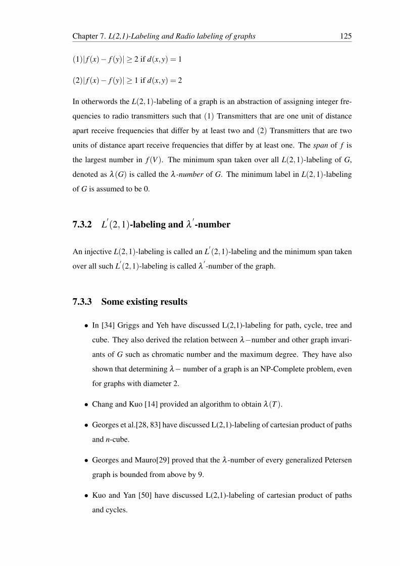
These cases are to be dealt separately. The L(2,1)-labeling for spl(Cn) when n = 4,5

are as shown in Figure 7.1

4

2

7 3

0

6

5

7

7 6

6

5

3

1 4

2

0

5

FIGURE 7.1: spl(C4),spl(C5) and its L(2,1)-labeling

Thus in all the possibilities R f = {0,1,2 . . . ,7} ⊂ N⋃{0}.

i.e. λ (spl(Cn)) = 7. �


Remark : The L(2,1)-labeling for spl(C3) is shown in Figure 7.2

Thus R f = {0,1,2 . . . ,6} ⊂ N⋃{0}.

6

65

0

24

FIGURE 7.2: spl(C3) and its L(2,1)-labeling

Illustration 7.4.2. Consider the graph spl(C6). The L(2,1)-labeling is as shown in

Figure 7.3.

0

2

4

0

2

4

7

6

5

7

6

5

FIGURE 7.3: spl(C6) and its L(2,1)-labeling

Theorem 7.4.3. λ′(spl(Cn)) = p− 1, where p is a total number vertices in spl(Cn)

(where n > 3).

Proof. Let v′1, v

′2, . . . , v

′n be the duplicated vertices corresponding to v1, v2, . . . , vn of

cycle Cn.

To define f : V (spl(Cn))−→ N⋃{0}, we consider following two cases.


Case 1: n > 5

f (vi) = 2i−7, 4≤ i≤ n

f (vi) = f (vn)+2i, 1≤ i≤ 3

f (v′i) = 2i−2, 1≤ i≤ n

Now label the vertices of C′n using the above defined pattern we have

R f = {0,1,2, . . . , p−1} ⊂ N⋃{0}

This implies that λ′(spl(Cn)) = p−1.

Case 2: n = 4,5 These cases to be dealt separately. The L′(2,1)-labeling for spl(Cn)

when n = 4,5 are as shown in the following Figure 7.4. �

1

0

7 2

6

4

5

5

9 3

7

1

4

8 2

6

0

3

FIGURE 7.4: spl(C4),spl(C5) and its L′(2,1)-labeling

Remark The L′(2,1)-labeling for spl(C3) is shown in the following Figure 7.5.

Thus R f = {0,1,2 . . . ,6} ⊂ N⋃{0}.

1

32

0

46

FIGURE 7.5: spl(C3) and its L′(2,1)-labeling


Illustration 7.4.4. Consider the graph spl(C6). The L′(2,1)-labeling is as shown in

Figure 7.6.

7

9

11

1

3

5

0

2

4

6

8

10

FIGURE 7.6: spl(C6) and its L′(2,1)-labeling

Theorem 7.4.5. Let C′n be the graph obtained by taking arbitrary supersubdivision of

each edge of cycle Cn then

1 For n even

λ (C′n) = ∆+2

2 For n odd

λ (C′n) =

∆+2; i f s+ t + r < ∆,

∆+3; i f s+ t + r = ∆,

s+ t + r+2; i f s+ t + r > ∆

where vk is a vertex with label 2,

s is number of subdivision between vk−2 and vk−1,

t is number of subdivision between vk−1 and vk,

r is number of subdivision between vk and vk+1,

∆ is the maximum degree of C′n.


Proof. Let v1, v2, . . . , vn be the vertices of cycle Cn. Let C′n be the graph obtained by

arbitrary super subdivision of cycle Cn.

It is obvious that for any two vertices vi and vi+2, N(vi)⋂

N(vi+2) = φ

To define f : V (C′n)−→ N

⋃{0}, we consider following two cases.

Case 1: n is even

f (v2i−1) = 0, 1≤ i≤ n2

f (v2i)= 1, 1≤ i≤ n2

If Pi j is the number of supersubdivisions between vi and v j then for the vertex v1,

|N(v1)| = P12 +Pn1. Without loss of generality we assume that v1 is the vertex with

maximum degree i.e. d(v1) = ∆. suppose u1,u2.....u∆ be the members of N(v1). We

label the vertices of N(v1) as follows.

f (ui) = 2+ i, 1≤ i≤ ∆

As N(v1)⋂

N(v3) = φ then it is possible to label the vertices of N(v3) using the vertex

labels of the members of N(v1) in accordance with the requirement for L(2,1)-labeling.

Extending this argument recursively upto N(vn−1) it is possible to label all the vertices

of C′n using the distinct numbers between 0 and ∆+2.

i.e. R f = {0,1,2, . . . ,∆+2} ⊂ N⋃{0}

Consequently λ (C′n) = ∆+2.

Case 2: n is odd

Let v1, v2, . . . , vn be the vertices of cycle Cn.

Without loss of generality we assume that v1 is a vertex with maximum degree and vk

be the vertex with minimum degree.

Define f (vk) = 2 and label the remaining vertices alternatively with labels 0 and 1 such

that f (v1) = 0. Then either f (vk−1) = 1 ; f (vk+1) = 0 OR f (vk−1) = 0 ; f (vk+1) = 1.

We assign labeling in such a way that f (vk−1) = 1 ; f (vk+1) = 0.

Now following the procedure adapted in case (1) it is possible to label all the vertices

except the vertices between vk−1 and vk. Label the vertices between vk−1 and vk using


the vertex labels of N(v1) except the labels which are used earlier to label the vertices

between vk−2, vk−1 and between vk, vk+1.

If there are p vertices u1,u2...up are left unlabeled between vk−1 and vk then label them

as follows,

f (ui)=max{labels of the vertices between vk−2 and vk−1, labels of the vertices between

vk and vk+1} + i, 1≤ i≤ p

Now if s is the number of subdivisions between vk−2 and vk−1

t is the number of subdivisions between vk−1 and vk

r is the number of subdivisions between vk and vk+1

then (1) R f = {0,1,2, . . . ,∆+2} ⊂ N⋃{0}, when s+ t + r < ∆

i.e. λ (C′n) = ∆+2

(2) R f = {0,1,2, . . . ,∆+3} ⊂ N⋃{0}, when s+ t + r = ∆

i.e. λ (C′n) = ∆+3

(3) R f = {0,1,2, . . . ,s+ t + r+2} ⊂ N⋃{0}, when s+ t + r > ∆

i.e. λ (C′n) = s+ t + r+2 �

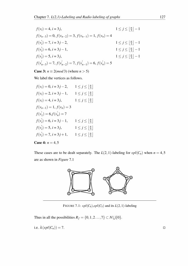
Illustration 7.4.6. Consider the graph C8. The L(2,1)-labeling of C′8 is shown in Figure

7.7.

345

6

5

67

0

1

1

0

1

0

1

0

78910

3

4

6

7

34

8

3

4

8

7

9

5

FIGURE 7.7: L(2,1)-labeling of C′8


Theorem 7.4.7. Let G′

be the graph obtained by taking arbitrary supersubdivision of

each edge of graph G with number of vertices n≥ 3 then λ′(G′) = p−1, where p is the

total number of vertices in G′.

Proof. Let v1, v2, . . . , vn be the vertices of any connected graph G and let G′

be the

graph obtained by taking arbitrary supersubdivision of G. Let uk be the vertices which

are used for arbitrary supersubdivision of the edge viv j where 1≤ i≤ n, 1≤ j ≤ n and

i < j. Here k is a total number of vertices used for arbitrary supersubdivision.

We define f : V (G′)−→ N

⋃{0} as

f (vi) = i−1, where 1≤ i≤ n

Now we label the vertices ui in the following order.

First we label the vertices between v1 and v1+ j, 1 ≤ j ≤ n then following the same

procedure for v2, v3,...vn

f (ui) = f (vn)+ i, 1≤ i≤ k

Now label the vertices of G′using the above defined pattern we have R f = {0,1,2, . . . , p−

1} ⊂ N⋃{0}

This implies that λ′(G′) = p−1. �

Illustration 7.4.8. Consider the graph P4 and its supersubdivision. The L′(2,1)-labeling

is as shown in Figure 7.8.

v1

v2 v3v41 2 30

4

5 8

6

12

11

10

9

7

FIGURE 7.8: L′(2,1)-labeling of P

′4


Theorem 7.4.9. Let C′n be the graph obtained by taking star of a cycle Cn then

λ (C′n) = 5.

Proof. Let v1, v2, . . . , vn be the vertices of cycle Cn and vi j be the vertices of cycle Cn

which are adjacent to the ith vertex of cycle Cn.

To define f : V (C′n)−→ N

⋃{0}, we consider following four cases.

Case 1: n≡ 0(mod 3)

f (vi) = 0, i = 3 j−2, 1≤ j ≤ n3

f (vi) = 2, i = 3 j−1, 1≤ j ≤ n3

f (vi) = 4, i = 3 j, 1≤ j ≤ n3

Now we label the vertices vi j of star of a cycle according to the label of f (vi).

(1) when f (vi) = 0, i = 3 j−2, 1≤ j ≤ n3

f (vik) = 3, k = 3p−2, 1≤ p≤ n3

f (vik) = 5, k = 3p−1, 1≤ p≤ n3

f (vik) = 1, k = 3p, 1≤ p≤ n3

(2) when f (vi) = 2, i = 3 j−1, 1≤ j ≤ n3

f (vik) = 5, k = 3p−2, 1≤ p≤ n3

f (vik) = 3, k = 3p−1, 1≤ p≤ n3

f (vik) = 1, k = 3p, 1≤ p≤ n3

(3) when f (vi) = 4, i = 3 j, 1≤ j ≤ n3

f (vik) = 1, k = 3p−2, 1≤ p≤ n3

f (vik) = 3, k = 3p−1, 1≤ p≤ n3

f (vik) = 5, k = 3p, 1≤ p≤ n3

Case 2: n≡ 1(mod 3)

f (vi) = 0, i = 3 j−2, 1≤ j ≤ bn3c

f (vi) = 2, i = 3 j−1, 1≤ j ≤ bn3c

f (vi) = 5, i = 3 j, 1≤ j ≤ bn3c

f (vn) = 3


Now we label the vertices of star of a cycle vi j according to label of f (vi).

(1) when f (vi) = 0, i = 3 j−2, 1≤ j ≤ bn3c

f (vik) = 4, k = 3p−2, 1≤ p≤ bn3c

f (vik) = 2, k = 3p−1, 1≤ p≤ bn3c

f (vik) = 0, k = 3p, 1≤ p≤ bn3c−1

f (vi(n−1)) = 5,

f (vin) = 1

(2) when f (vi) = 2, i = 3 j−1, 1≤ j ≤ bn3c

f (vik) = 4, k = 3p−2, 1≤ p≤ bn3c

f (vik) = 0, k = 3p−1, 1≤ p≤ bn3c

f (vik) = 2, k = 3p, 1≤ p≤ bn3c−1

f (vi(n−1)) = 3,

f (vin) = 1

(3) when f (vi) = 5, i = 3 j, 1≤ j ≤ bn3c

f (vik) = 1, k = 3p−2, 1≤ p≤ bn3c

f (vik) = 3, k = 3p−1, 1≤ p≤ bn3c

f (vik) = 5, k = 3p, 1≤ p≤ bn3c−1

f (vi(n−1)) = 0,

f (vin) = 4

(4) when f (vi) = 3, i = n

f (vik) = 1, k = 3p−2, 1≤ p≤ bn3c

f (vik) = 5, k = 3p−1, 1≤ p≤ bn3c

f (vik) = 3, k = 3p, 1≤ p≤ bn3c−1

f (vi(n−1)) = 0

f (vin) = 4


Case 3: n≡ 2(mod 3), n , 5

f (vi) = 1, i = 3 j−2, 1≤ j ≤ bn3c−1

f (vi) = 3, i = 3 j−1, 1≤ j ≤ bn3c−1

f (vi) = 5, i = 3 j, 1≤ j ≤ bn3c−1

f (vn−4) = 0, f (vn−3) = 2,

f (vn−2) = 5, f (vn−1) = 0, f (vn) = 4

Now we label the vertices vi j of star of a cycle according to the label of f (vi).

(1) when f (vi) = 1, i = 3 j−2, 1≤ j ≤ bn3c−1

f (vik) = 5, k = 3p−2, 1≤ p≤ bn3c

f (vik) = 3, k = 3p−1, 1≤ p≤ bn3c

f (vik) = 1, k = 3p, 1≤ p≤ bn3c

f (vi(n−1)) = 4,

f (vin) = 0

(2) when f (vi) = 3, i = 3 j−1, 1≤ j ≤ bn3c−1

f (vik) = 0, k = 3p−2, 1≤ p≤ bn3c

f (vik) = 2, k = 3p−1, 1≤ p≤ bn3c

f (vik) = 4, k = 3p, 1≤ p≤ bn3c

f (vi(n−1)) = 1,

f (vin) = 5

(3) when f (vi) = 5, i = 3 j, 1≤ j ≤ bn3c−1 and i = n−2

f (vik) = 1, k = 3p−2, 1≤ p≤ bn3c

f (vik) = 3, k = 3p−1, 1≤ p≤ bn3c

f (vik) = 5, k = 3p, 1≤ p≤ bn3c

f (vi(n−1)) = 2,

f (vin) = 4


(4) when f (vi) = 0, i = n−4,n−1

f (vik) = 3, k = 3p−2, 1≤ p≤ bn3c

f (vik) = 5, k = 3p−1, 1≤ p≤ bn3c

f (vik) = 1, k = 3p, 1≤ p≤ bn3c−1

f (vi(n−2)) = 2,

f (vi(n−1)) = 4,

f (vin) = 1

(5) when f (vi) = 2, i = n−3

f (vik) = 4, k = 3p−2, 1≤ p≤ bn3c

f (vik) = 0, k = 3p−1, 1≤ p≤ bn3c

f (vik) = 2, k = 3p, 1≤ p≤ bn3c

f (vi(n−1)) = 5,

f (vin) = 1

(6) when f (vi) = 4, i = n

f (vik) = 2, k = 3p−2, 1≤ p≤ bn3c

f (vik) = 0, k = 3p−1, 1≤ p≤ bn3c

f (vik) = 4, k = 3p, 1≤ p≤ bn3c

f (vi(n−1)) = 1,

f (vin) = 5

Case 4: n = 5 This case is to be dealt separately. The L(2,1)-labeling for the graph

obtained by taking star of the cycle C5 is shown in Figure 7.9 .


0

2

51

4

4 0

5

3

1

02

5

1

4

2

4

1

3

03

5

1

4

0

2

51

4

0

FIGURE 7.9: L(2,1)-labeling for star of cycle C5

Thus in all the possibilities we have λ (C′n) = 5 �

Illustration 7.4.10. Consider the graph C7, the L(2,1)-labeling is as shown in Figure

7.10.

42

5

1

4

4

0

2

4

5

1

4

0

2 4

0

3

1

4

0

24

0

3

1

1

53

1

5 0

4

1

35

1

3

0 4

1

3 5

1

30

4

2

02

5

02

5

3

2

0

FIGURE 7.10: L(2,1)-labeling for star of cycle C7


Theorem 7.4.11. Let G′be the graph obtained by taking star of a graph G then λ

′(G′) =

p−1, where p be the total number of vertices of G′.

Proof. Let v1, v2, . . . , vn be the vertices of any connected graph G. Let vi j be the vertices

of a graph which is adjacent to the ith vertex of graph G. By the definition of a star of a

graph the total number of vertices in a graph G′are n(n+1).

To define f : V (G′)−→ N

⋃{0}

f (vi1) = i−1, 1≤ i≤ n

for 1≤ i≤ n do the labeling as follows:

f (vi) = f (vni)+1

f (v1(i+1)) = f (vi)+1

f (v( j+1)(i+1)) = f (v j(i+1))+1, 1≤ j ≤ n−1

Thus λ′(G′) = p−1 = n2 +n−1 �

Illustration 7.4.12. Consider the star of a graph K4, the L′(2,1)-labeling is as shown in

Figure 7.11.

14 19

3 8

1318712

17 2

9 4

5 10

150

11 16

6 1

FIGURE 7.11: L′(2,1)-labeling for star of a complete graph K4


7.5 Radio labeling of graph

We have discussed the L(2,1)-labeling in previous section. Practically it has been

observed that the interference among channels might go beyond two levels. Radio la-

beling extends the number of interference level considered for L(2,1)-labeling from two

to the largest possible - the diameter of G. Motivated through the problem of channel

assignments to FM radio stations Chartrand et al.[15] introduced the concept of radio

labeling of graph as follows.

7.5.1 Radio labeling

A radio labeling of a graph G is an injective function f : V (G) −→ N ∪{0} such that

for every u,v ∈V

| f (u)− f (v)| ≥ diam(G)−d(u,v)+1

The span of f is the difference of the largest and the smallest channels used. That is,

max( f (u), f (v)), for every u,v ∈V

The radio number of G is defined as the minimum span of a radio labeling of G and

denoted as rn(G). In the survey of literature available on radio labeling we found that

only two types of problems are considered in this area till this date.

• To investigate bounds for the radio number of a graph.

• To completely determine the radio number of a graph.

7.5.2 Some existing results

• Chartrand et al.[15] and Liu and Zhu[52] have discussed the radio number for

paths and cycles.

• D.D-F Liu [53] has discuss radio number for trees.

• D.D-F.Liu and M.Xie[54] have discussed radio number of square of cycles.


• Mustapha et al.[47] have discussed radio k-labeling for cartesian products of

graphs.

• Sooryanarayana et al.[64] have discussed radio number of cube of a path.

7.6 Radio labeling for some cycle related graphs

Theorem 7.6.1. Let G be the cycle with chords then.'

i i

'i i

n 'i i

'i i

(k+2)(2k-1)+1+ (d - d ). n 0 (mod 4)

2k(k+2)+1+ (d - d ). n 2 (mod 4)

r (G)2k(k+1)+ (d - d ). n 1 (mod 4)

(k+2)(2k+1)+ (d - d ). n 3 (mod 4)

i

i

i

i

ì ºïï ºïï

£ íºï

ïï ºïî

å

å

å

å

Proof. Let Cn denote the cycle on n vertices and V (Cn) = {v0,v1 . . .vn−1} be such that

where vi is adjacent to vi+1 and vn−1 is adjacent to v0. We denote d = diam(Cn).

Here the radio labeling of a cycle Cn is given by the following two sequences.

• the distance gap sequence D = (d0,d1 . . .dn−2)

• the color gap sequence F = ( f0, f1 . . . fn−2)

The distance gap sequence in which each di ≤ d is a positive integer is used to generate

an ordering of the vertices of Cn. Let τ : {0,1, . . . ,n−1}−→{0,1, . . . ,n−1} be defined

as τ(0) = 0 and τ(i+ 1) = τ(i)+ di (mod n). Here τ is a corresponding permutation.

Let xi = vτ(i) for i = 0,1,2, . . .n− 1 then {x0,x1 . . .xn−1} is an ordering of the vertices

of Cn. Let us denote d(xi,xi+1) = di.

The color gap sequence is used to assign labels to the vertices of Cn. Let f be the la-

beling defined by f (x0) = 0 and for i ≥ 1, f (xi+1) = f (xi)+ fi. By definition of radio

labeling fi ≥ d− di + 1 for all i. We adopt the scheme for distance gap sequence and

color gap sequence reported in [52] and proceed as follows.


Case 1: n = 4k in this case diam(G) = 2k

Using the sequences given below we can generate the radio labeling of cycle Cn for

n≡ 0(mod 4)with minimum span.

The distance gap sequence is given by

di = 2k if i is even

= k if i≡ 1(mod 4)

= k+1 if i≡ 3(mod 4)

and the color gap sequence is given by

fi = 1 if i is even

= k+1 if i is odd

Then for i = 0,1,2, . . .k−1 we have the following permutation,

τ(4i) = 2ik+ i(mod n)

τ(4i+1) = (2i+2)k+ i(mod n)

τ(4i+2) = (2i+3)k+ i(mod n)

τ(4i+3) = (2i+1)k+ i(mod n)

Now we add chords in cycle Cn such that diameter of cycle remain unchanged. Label

the vertices of this newly obtained graph using above permutation. Suppose the new

distance between xi and xi+1 is d′i(xi,xi+1) then due to chords in the cycle it is obvious

that di ≥ d′i .

We define the color gap sequence as

f′i = fi +(di−d

′i), 0≤ i≤ n−2

So, that span f′for cycle with chords is

f′0 + f

′1 . . .+ f

′n−2 = f0 + f1 + f2 . . .+ fn−2 +∑(di−d

′i)

= rn(Cn)+∑(di−d′i)

=(k+2)(2k−1)+1+∑(di−d′i). 0≤ i≤ n−2

which is an upper bound for radio number for cycle with arbitrary number of chords

when n = 4k.

Case 2: n = 4k+2 in this case diam(G) = 2k+1

Using the sequences given below we can generate radio labeling of cycle Cn for


n≡ 2(mod 4) with minimum span.


di = 2k+1 if i is even

= k+1 if i is odd


fi = 1 if i is even

= k+1 if i is odd

Hence for i = 0,1, . . .2k, we have the following permutation,

τ(2i) = i(3k+2) (mod n)

τ(2i+1) = i(3k+2)+2k+1 (mod n)

Now we add chords in cycle Cn such that diameter of cycle remain unchanged. Label

the vertices of this newly obtained graph by using the above permutation. So, that span

f′for cycle with chords is

f′0 + f

′1 . . .+ f

′n−2 = f0 + f1 + f2 . . .+ fn−2 +∑(di−d

′i)


= 2k(k+2)+1+∑(di−d′i). 0≤ i≤ n−2

which is an upper bound for radio number for cycle with arbitrary number of chords.

when n = 4k+2

Case 3: n = 4k+1 in this case diam(G) = 2k

Using the sequences given below we can generate radio labeling of cycle Cn for n ≡

1(mod 4) with minimum span.


d4i = d4i+2 = 2k− i

d4i+1 = d4i+3 = k+1+ i


fi = 2k−di +1


Then we have

τ(2i) =i(3k+1) (mod n), 0≤ i≤ 2k

τ(4i+1) = 2(i+1)k (mod n), 0≤ i≤ k−1

τ(4i+3) = (2i+1)k (mod n), 0≤ i≤ k−1

Label the vertices of this newly obtained graph by using the above permutation. So, that

span of f′for cycle with chords is

f′0 + f

′1 . . .+ f

′n−2 = f0 + f1 + f2 . . .+ fn−2 +∑(di−d

′i)


= 2k(k+1)+∑(di−d′i). 0≤ i≤ n−2

which is an upper bound for radio number for cycle with arbitrary number of chords.

when n = 4k+1

Case 4: n = 4k+3 in this case diam(G) = 2k+1

Using the sequences below we can give radio labeling of cycle Cn for n ≡ 3(mod 4)

with minimum span.


d4i = d4i+2 = 2k+1− i

d4i+1 = k+1+ i

d4i+3 = k+2+ i


fi = 2k−di +2 if i . 3(mod 4)

= 2k−di +3 otherwise

Then we have the following permutation,

τ(4i) = 2i(k+1) (mod n) , 0≤ i≤ k

τ(4i+1) = (i+1)(2k+1) (mod n) , 0≤ i≤ k

τ(4i+2) = (2i−1)(k+1) (mod n) , 0≤ i≤ k

τ(4i+3) = i(2k+1)+ k (mod n), 0≤ i≤ k−1, 1≤ i≤ n−2

Label the vertices of this newly obtained graph by following the above permutation. So,

that span of f′for cycle with chords is


f′0 + f

′1 . . .+ f

′n−2 = f0 + f1 + f2 . . .+ fn−2 +∑(di−d

′i)


= (k+2)(2k+1)+∑(di−d′i)

which is an upper bound for radio number for cycle with arbitrary number of chords for

the cycle with chords.

Thus in all the possibilities we have obtained the upper bounds of the radio numbers. �

Illustration 7.6.2. Consider the graph C12 with 5 chords, the radio labeling is as shown

in Figure 7.12.

x00

42

27

6

38

17

243

25

10

32

21

x5

x8

x3

x6

x11 x

1

x4

x9

x2

x7

x10

ordinary labeling for cycle with chords

Radio labeling for cycle with chords for C12

FIGURE 7.12: ordinary and radio labeling for cycle with chords for C12

Theorem 7.6.3. Let G be n/2-petal graph then

rn(G)≤

3p2 +n

⌊n4

⌋−⌊n

8

⌋−2n−2

(p−1)+n⌊n

4

⌋−⌊n

8

⌋+2n

Proof. Let G be n/2-petal graph with v0,v1 . . .vn−1 vertices of degree 3 and v′1,v

′2 . . .v

′p

vertices of degree 2. Here vi is adjacent to vi+1 and vn−1 is adjacent to v0.


Case 1: n≡ 0(mod4) and diam(G) = bn/4c+2

First we label the vertices of degree 2. Let v′1,v

′2 . . .v

′p be the vertices on the petals

satisfying the order define by following distance sequence.

d′i = bn/4c+2 if i is even

= bn/4c+1 if i is odd

The color gap sequence for vertices on petals is defined as

f′i = 1 if i is even

= 2 if i is odd

Let v1 be the vertex on the cycle Cn such that d(v′p,v1) = bn/8c+1 = d(v

′p−1,v1)

then label v1 as f (v1) = f (v′p)+diam(G)−bn/8c

Now for the remaining vertices of degree 3 we use the permutation defined for the cycle

Cn in case 1 of Theorem 7.6.1.

and the color gap sequence for the same vertices is defined as

fi = bn/4c+2, 0≤i≤ n−2

Then span of f = 3p/2+nbn/4c−bn/8c−2n−2.

Which is an upperbound for the radio number of n/2-petal graph when n≡ 0(mod4).

Case 2: n≡ 2(mod4) and diam(G) = bn/4c+2

First we label the vertices of degree 2. Let v′1,v

′2 . . .v

′p be the vertices on the petals

satisfying the order define by following distance sequence.

d(v′i,v′i+1) = bn/4c+2

The color gap sequence for the vertices on the petals is defined as

f′i = 1,1≤ i≤ p

Let v1 be the vertex on the cycle Cn such that d(v′p,v1) = bn/8c+1 = d(v

′p−1,v1)

then label v1 as f (v1) = f (v′p)+diam(G)−bn/8c

Now for the remaining vertices of degree 3 we use the permutation defined for the cycle

Cn in case 2 of Theorem 7.6.1.

and the color gap sequence for the same vertices is defined as

fi = bn/4c+2, 0≤i≤ n−2

Then span of f = p−1+nbn/4c−bn/8c+2n.

Which is an upperbound for the radio number of n/2-petal graph when n ≡ 2(mod4).

�


Illustration 7.6.4. Consider the n/2-petal graph of C8. The radio labeling is shown in

Figure 7.13.

Ordinary labeling for n/2-petalgraph of C

x0

x1

x2x6

x3

x5

x0

x7x

2

x4

x1

x3

0

1

3

4

7

27

19

31

11

23

15

35

Radio labeling for n/2 - petal graph of C88

'

'

'

'

FIGURE 7.13: ordinary and radio labeling for a n/2-petal graph of C8

Theorem 7.6.5.

rn(spl(Cn)) =

2[(k+2)(2k−1)+1]+ k+1 n ≡ 0(mod 4)

2[2k(k+2)+1]+ k+1 n≡ 2(mod 4)

2[2k(k+1)] + k+1 n≡ 1(mod 4)

2[(k+2)(2k+1)]+ k+1 n≡ 3(mod 4)

Proof. Let v′1,v

′2,v

′3 . . .v

′n be the duplicated vertices corresponding to v1,v2,v3 . . .vn. As

d(vi,v j) = d(vi,v′j) and in order to obtain the labeling with minimum span we employ

twice the distance gap sequence, the color gap sequence and the permutation scheme

used in [52]. First we label the vertices of cycle and then their duplicated vertices.

Case 1: n≡ 4k(n > 4)then diam(G) = 2k

We first label the vertices v1,v2,v3 . . .vn as according to Case 1 of Theorem 7.6.1 and

then we label the vertices v′1,v

′2,v

′3 . . .v

′n as follows.

Define f (v′j) = f (vn−1)+ k+1 where v

′j be the vertex such that d(vn−1,v

′j) = k

Now with permutation scheme used in Case 1 of Theorem 7.6.1 for cycle n≡ 0(mod 4)

label the duplicated vertices starting from v′j.


Then rn(spl(Cn))= f0 + f1 + f2 . . .+ fn−2 +2k− k+1+ f′0 + f

′1 + · · ·+ f

′n−2

As fi = f′i , for i = 0,1,2 . . .n−2, then

rn(spl(Cn)) = 2 f0 +2 f1 +2 f2 . . .+2 fn−2 + k+1

= 2[(k+2)(2k−1)+1]+ k+1

Case 2: n≡ 4k+2(n > 6) then diam(G) = 2k+1

We first label the vertices v1,v2,v3 . . .vn according to Case 2 of Theorem 7.6.1 and then

we label the vertices v′1,v

′2,v

′3 . . .v

′n as follows.

Define f (v′j) = f (vn−1)+1 where v


′j) = k+1

Now with permutation for cycle n ≡ 2(mod 4) used in Case 2 of Theorem 7.6.1 label

the duplicated vertices starting from v′j.

Then rn(spl(Cn))= f0 + f1 + f2 . . .+ fn−2 +2k+1− k−1+1+ f′0 + f

′1 + · · ·+ f

′n−2


rn(spl(Cn)) =2 f0 +2 f1 +2 f2 . . .+2 fn−2 + k+1

= 2[2k(k+2)+1]+ k+1

Case 3: n≡ 4k+1(n > 5) then diam(G) = 2k

We first label the vertices v1,v2,v3 . . .vn as defined in Case 3 of Theorem 7.6.1. Now


′2,v

′3 . . .v

′n as follows.

Define f (v′j) = f (vn−1)+ k where v


′j) = k+1



Then rn(spl(Cn))= f0 + f1 + f2 . . .+ fn−2 +2k− k−1+1+ f′0 + f

′1 + · · ·+ f

′n−2


rn(spl(Cn)) =2 f0 +2 f1 +2 f2 . . .+2 fn−2 + k+1

= 2[2k(k+1)]+ k+1

Case 4: n≡ 4k+3(n > 3) then diam(G) = 2k+1

We first label the vertices v1,v2,v3 . . .vn as defined in Case 4 of Theorem 7.6.1. Now


′2,v

′3 . . .v

′n as follows.

v′j be the vertex such that d(vn−1,v

′j) = k+1

Define f (v′j) = f (vn−1)+ k+1 where v


′j) = k+1




Then rn(spl(Cn))= f0 + f1 + f2 . . .+ fn−2 +2k+1− k−1+1+ f′0 + f

′1 + · · ·+ f

′n−2


rn(spl(Cn)) =2 f0 +2 f1 +2 f2 . . .+2 fn−2 + k+1

= 2[(k+2)(2k+1)]+ k+1

Thus in all the four possibilities we have determined radio number of graph G under

consideration. �

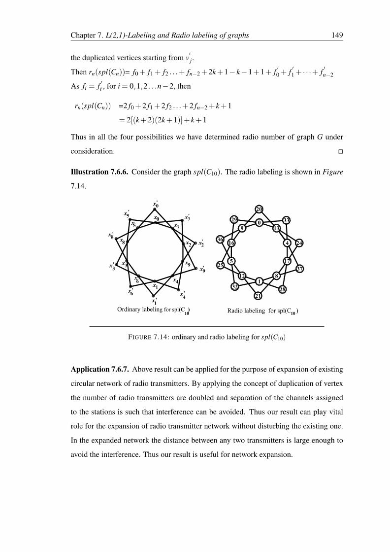
Illustration 7.6.6. Consider the graph spl(C10). The radio labeling is shown in Figure

7.14.

013

4

17

81

12

5

16

9

20

33

24

37

2821

32

25

36

29x

x

x

x

xx

x

x

xx

x

x

x

x x

xx

x

x

0

1

1

4

4

99

2

7

7

05

5

88

33

6

6

x2

'

'

'

'

'

'

'

'

'

'

Ordinary labeling for spl(C ) Radio labeling for spl(C )10 10

FIGURE 7.14: ordinary and radio labeling for spl(C10)

Application 7.6.7. Above result can be applied for the purpose of expansion of existing

circular network of radio transmitters. By applying the concept of duplication of vertex

the number of radio transmitters are doubled and separation of the channels assigned

to the stations is such that interference can be avoided. Thus our result can play vital

role for the expansion of radio transmitter network without disturbing the existing one.

In the expanded network the distance between any two transmitters is large enough to

avoid the interference. Thus our result is useful for network expansion.


Theorem 7.6.8. rn(M(Cn)) =

2(k+2)(2k−1)+n+3 n≡ 0(mod 4)

4k(k+2)+ k+n+3 n≡ 2(mod 4)

4k(k+1)+ k+n n≡ 1(mod 4)

2(k+2)(2k+1)+ k+n+1 n≡ 3(mod 4)

Proof. Let u1,u2, . . . ,un be the vertices of the cycle Cn and u′1,u

′2, . . . ,u

′n be the newly

inserted vertices corresponding to the edges of Cn to obtain M(Cn). In M(Cn) the diam-

eter is increased by 1.

Here d(ui,u j)≥ d(ui,u′j) for n≡ 0,2(mod 4) and d(ui,u j)= d(ui,u

′j) for n≡ 1,3(mod 4).

Through out the discussion first we label the vertices u1,u2, . . . ,un and then newly in-

serted vertices u′1,u

′2, . . . ,u

′n. For this purpose we will employ twice the permutation

scheme for respective cycle as in considered in Theorem 7.6.1.

Case 1: n≡ 4k in this case diam(M(Cn)) = 2k+1

The distance gap sequence to order the vertices of original cycle Cn is defined as follows

because fi + fi+1 ≤ f′i + f

′i+1, for all i


= k+1 if i≡ 1(mod 4)

= k+2 if i≡ 3(mod 4)

The color gap sequence is defined as follows

fi = 1 if i is even

= k+1 if i is odd

Let u′1 be the vertex on the inscribed cycle such that d(un,u

′1) = k+1 and f = k+1

The distance gap sequence to order the vertices of the inscribed cycle Cn is defined as

follows

di = 2k if i is even

= k if i≡ 1(mod 4)

= k+1 if i≡ 3(mod 4)


The color gap sequence is defined as follows


= k+2 if i≡ 1(mod 4)

= k+1 if i≡ 3(mod 4)

Thus in this case rn(M(Cn)) = 2(k+2)(2k−1)+n+3

Case 2: n = 4k+2 in this case diam(M(Cn)) = 2k+2



′i+1, for all i


= k+3 if i is odd


fi = 1 if i is even

= k+1 if i is odd


′1) = k+1 and f = k+2


followsdi = 2k+1 if i is even

= k+1 if i is odd



= k+2 if i is odd

Thus rn(M(Cn)) = 4k(k+2)+ k+n+3




′i+1, for all i

d4i = d4i+2 = 2k+1− i

d4i+1 = d4i+3 = k+2+ i


fi = (2k+1)−di +1


′1) = k+1 and f = k+1



follows

d4i = d4i+2 = 2k− i

d4i+1 = d4i+3 = k+1+ i


f′i = 2k−di +2

Thus in this case rn(M(Cn)) = 4k(k+1)+ k+n




′i+1, for all i

d4i = d4i+2 = 2k+2− i

d4i+1 = d4i+3 = k+2+ i


fi= 2k−di +3


′1) = k+2 and f = k+1

The distance gap sequence to order the vertices of inscribed cycle Cn is defined as fol-

lows

d4i = d4i+2 = 2k+1− i

d4i+1 = k+1+ i

d4i+3 = k+2+ i


f′i = 2k−di +3

Thus in this case rn(M(Cn)) = 2(k+2)(2k+1)+n

Thus the radio number is completely determined for the graph M(Cn). �


Illustration 7.6.9. consider the graph M(C8). The radio labeling is shown in Figure

7.15.

x0

x7

x2

x4

x1

x6

x3

x5

x0'

x7'

x2'

x4'

x1'

x6'x3

'

x5'

0

1

45

8

9

12

13

16

18

22

24

27

29

33

35

Ordinary labeling for M(C ) 8 Radio labeling for M(C ) 8

FIGURE 7.15: ordinary and radio labeling of M(C8)

Application 7.6.10. Above result is possibly useful for the expansion of existing radio

transmitters network. In the expanded network two newly installed nearby transmitters

are connected and interference is also avoided between them. Thus the radio labeling

described in above Theorem 7.6.8 is rigourously applicable to accomplish the task of

channel assignment for the feasible network.

7.6.11. The comparison between Radio numbers of Cn, spl(Cn) and M(Cn) is tabulated

in the following Table 1.

Table 1 Comparison of radio numbers of Cn , spl(Cn) and M(Cn)


7.7 Concluding Remarks and Scope of Further Research

The L(2,1)-labeling and the Radio labeling are the labelings which concern to

channel assignment problem. The lowest level of interference will make the enter-

tainment meaningful and enjoyable. The expansion of network is also demand of the

recent time. The investigations reported in this chapter will serve both of these pur-

poses. Our investigations can be applied for network expansion without disturbing the

existing network. To develop such results for various graph families is an open area of

research.

discussion on some interesting topics in graph theory

Documents