UNEMPLOYMENT AND REAL WAGES IN WEIMAR GERMANY

N. H. DIMSDALE, N. HORSEWOOD, and A. VAN RIEL

U N I V E R S I T Y O F O X F O R D

Discussion Papers in

Economic and Social History

Number 56, October 2004

U N I V E R S I T Y O F O X F O R D

Discussion Papers in Economic and Social History

1 Hans-Joachim Voth and Tim Leunig, Did Smallpox Reduce Height? Stature and the Stan-dard of Living in London, 1770–1873 (Nov. 1995)

2 Liam Brunt, Turning Water into Wine – New Methods of Calculating Farm Output and New Insights into Rising Crop Yields during the Agricultural Revolution (Dec. 1995)

3 Avner Offer, Between the Gift and the Market: the Economy of Regard (Jan. 1996)

4 Philip Grover, The Stroudwater Canal Company and its Role in the Mechanisation of the Gloucestershire Woollen Industry, 1779–1840 (March 1996)

5 Paul A. David, Real Income and Economic Welfare Growth in the Early Republic or, An-other Try at Getting the American Story Straight (March 1996)

6 Hans-Joachim Voth, How Long was the Working Day in London in the 1750s? Evidence from the Courtroom (April 1996)

7 James Foreman-Peck, ‘Technological Lock-in’ and the Power Source for the Motor Car (May 1996)

8 Hans-Joachim Voth, Labour Supply Decisions and Consumer Durables During the Indus-trial Revolution (June 1996)

9 Charles Feinstein, Conjectures and Contrivances: Economic Growth and the Standard of Living in Britain During the Industrial Revolution (July 1996)

10 Wayne Graham, The Randlord’s Bubble: South African Gold Mines and Stock Market Manipulation (August 1996)

11 Avner Offer, The American Automobile Frenzy of the 1950s (December 1996)

12 David M. Engstrom, The Economic Determinants of Ethnic Segregation in Post-War Britain (January 1997)

13 Norbert Paddags, The German Railways – The Economic and Political Feasibility of Fiscal Reforms During the Inflation of the Early 1920s (February 1997)

14 Cristiano A. Ristuccia, 1935 Sanctions against Italy: Would Coal and Crude Oil have made a Difference? (March 1997)

15 Tom Nicholas, Businessmen and Land Purchase in Late Nineteenth Century England (April 1997)

16 Ed Butchart, Unemployment and Non-Employment in Interwar Britain (May 1997)

17 Ilana Krausman Ben-Amos, Human Bonding: Parents and their Offspring in Early Modern England (June 1997)

18 Dan H. Andersen and Hans-Joachim Voth, The Grapes of War: Neutrality and Mediterra-nean Shipping under the Danish Flag, 1750–1802 (September 1997)

[Continued inside the back cover]

UNEMPLOYMENT AND REAL WAGES IN WEIMAR GERMANY

N. H. DIMSDALE The Queen’s College, Oxford

N. HORSEWOOD Department of Economics, University of Birmingham

A. VAN RIEL Social Policy, Netherlands Economic Institute, Rotterdam

Abstract This paper contributes to the debate on the causes of unemployment in interwar Ger-many. It applies the Layard-Nickell model of the labour market to interwar Germany, using a new quarterly data set. The basic model is extended to capture the effects of the tariff wage under the Weimar Republic and the Nazis. The estimated equations suggest that demand shocks, combined with nominal inertia in the labour market, were important in explaining unemployment. In addition real wage pressures due the political processes of wage determination were a major influence on unemployment. Negative demand shocks appear to have been initially domestic and to have started before the impact of the World Depression. Both negative developments on the demand side of the economy and pressures coming from the supply side raised unemployment in the slump. In the re-covery the wage policies of the Nazis and the revival of demand both contributed to the fall in unemployment. The mutual reinforcement of these factors may help to explain the severity of the interwar cycle in Germany. It also serves to emphasize the close connec-tion between political and economic processes in this important episode in macroeco-nomic history. JEL classification: N14, E24, E32

Keywords: Great Depression, Germany, real wages, unemployment

Acknowledgements: We acknowledge with gratitude the comments of Peter Temin and Joachim Voth on earlier drafts of the paper. We received helpful suggestions from participants in the Berlin Colloquium on Quantitative History held in September 2004 and in particular we thank Albrecht Ritschi for his encouragement.

Corresponding author with email address: <nicholas.dimsdale@queens.ox.ac.uk>

3

I. Introduction

Germany’s experience of the Great Depression was exceptionally severe. Between the summer of 1929 and early 1932, German unemployment rose from just under 1.3 million to over 6 million, corresponding to a rise in the unemployment rate from 4.5 per cent of the labour force to 24 per cent. Following a seasonal upswing in labour demand, reducing the level to 5.1 million in September 1932, unemployment again exceeded 6 million at the start of 1933.1 Over the same period real GDP, according to the latest estimates, declined at an annual rate of 8.3 per cent. Real weekly wages, having continued to rise up to early 1931, started a decline of 2.5 per cent per annum that lasted until mid 1935. In short the German slump was the most dramatic among major European economies.2

As the economic crisis unfolded, the first German Republic suffered the decline of its democratic institutions. As the country was ruled by a series minority cabinets and presi-dential decrees, the share of the vote at successive elections shifted in favour of the Com-munist and Nazi opposition parties, rising from 13 per cent under the last parliamentary coalition government in May 1928 to half of all valid votes cast in the last free elections of November 1932.3 On January 30 1933 the Reichspräsident, after an earlier refusal in 1932, appointed Adolf Hitler as the chancellor of a Nazi dominated coalition, setting the nation upon a path of totalitarian rule, warfare and racial persecution. Thus the dismal re-cord of the German economy in the interwar period holds a pivotal position in the analysis of the political demise of the Weimar Republic. Ranking among the world’s most dynamic economies in the years before World War I, Germany experienced successively inflation and severe deflation during the 1920s and the early 1930s. Both events undermined the al-ready questionable legitimacy of what has been called the improvised Republic and created the conditions for the emergence of political radicalization.4

Successive authors have differed in their assessment of the relevant mechanisms at work and on the extent to which the monetary and political events of the 1920s made Ger-many vulnerable to the impact of the Great Depression. Early studies of the Weimar decline did not emphasize the interaction of political and economic processes. A passing reference

1 For sources, see Data Appendix. 2 Quarterly estimates of GDP are from Ritschl (1999a). 3 Election statistics are from Falter et al. (1986). The connection between voting patterns and unem-ployment is explored in van Riel and Schram (1993). 4 Eschenberg (1984).

4

was made to the effects of the economic crisis in what was seen as a process of decline in democratic rule. Starting with Bracher (1954), this literature was mainly concerned with the constitutional arrangements of the post-World War I federal state and the vulnerability of its institutions to the erosion of parliamentary rule. The instability of successive coalitions was seen as a manifestation of an ill-adapted parliamentary system, threatened by economic turbulence and deep social divisions.5

The critical role of economic policy during the Depression was emphasized during the period when Keynesian views were dominant. The deflationary policies of Brüning were at-tacked by those arguing the case for fiscal expansion.6 The principal line of defence against this critique was that policy makers chose to subordinate fiscal policy to reparations policy with the aim of lifting the constraints on borrowing. There was also a natural prudence in German economic policy during the Great Depression in the light of the inflationary ex-periences of the early 1920s. Both these justifications for Weimar economic policy were put forward by Brüning in his memoirs (Brüning 1970).

The postwar consensus blamed the policy choices of the Brüning cabinet for the disas-trous economic and political outcome of the Weimar regime. As Balderston (1993) states: ‘received opinion up to 1979 viewed the slump in Germany as the result of a combination of monetary instability and policy inaptness’.7 This consensus was challenged by the Mu-nich historian Knut Borchardt [1979] (1991a), who related the structural weakness in Ger-many’s economic performance in the 1920s, based of Hoffman’s national income data,8 to the political difficulties of the Weimar Republic. He argued that there was a structural defi-ciency in the German economy, which was present before the onset of the slump and was related to weak productivity performance, increasing money wages and under investment. During the post inflation period wage increases based on institutionalized arbitration were claimed to have exceeded the growth of labour productivity, squeezing profits and discour-aging investment. Monetary restraint, rooted in reparations po licy under the Young Plan with its reliance upon the gold standard, severely restricted the freedom of action of Wei-mar governments as did the limited creditworthiness of the German state. According to this view, Brüning had no room for manoeuvre leaving no practical alternative to deflation.

5 Heiber (1966). 6 See Erbe (1958), Sanmann (1965). 7 Balderston (1993), pp. 4–5. 8 Borchardt (1991a), Hoffman et al. (1965).

5

Balderston (2002) has usefully distinguished between the Borchardt I hypothesis, which relates to the effects of labour market pressures on the Weimar economy, and the Bor-chardt II hypothesis, which questions whether there were any realistic alternatives to the policy of deflation in 1931.9 In this paper we are primarily interested in the first hypothesis, taking as our starting point Borchardt’s concise statement of the main issue:

Neither economic theory nor empirical evidence appears to me to have deliv-ered clear criteria for answering the question as to whether continuing unem-ployment was a case of weakness in demand or whether this was a case of classical real wage unemployment, or perhaps both factors played a part.10

Our aim in this paper is to seek to resolve this issue but we do not restrict ourselves to the late 1920s and analyse a sample running from 1926 to 1936. We use the model of the aggregate labour market developed by Layard and Nickell. It was proposed initially to ex-plain unemployment in postwar Britain in Layard and Nickell (1986) and this aim was ex-tended to a full analysis of the working of postwar labour markets in OECD countries in Layard, Nickell and Jackman (1991). The model was used to explain British interwar ex-perience in Dimsdale, Nickell and Horsewood (1989) and more recently has been applied to the Australian labour market in the interwar period in Dimsdale and Horsewood (2002). The model seeks to distinguish between the impact of demand- and supply-side factors on unemployment and so is well suited to responding to the issue which Borchardt has raised. It is also consistent with both bargaining and efficiency wage modelling of the labour mar-ket at the micro level. It should therefore be flexible enough to cope with the switch of re-gime from Weimar to the Nazis. We have extended the model to take account of the rela-tionship between the market wage and the contract or tariff wage. This enables us to exam-ine the role of political and economic factors in explaining wages, an issue raised by both Borchardt (1990, 1991b)11 and Balderston (1983).12

We are able to undertake this empirical work because of substantial improvements to the quarterly data for the interwar German economy, which are fully described in the Appendix. We are chiefly interested in the German slump, but as the sample covers the period 1926–36, we can also examine the factors explaining the initial stages of the recovery under the

9 Balderston (2002), pp. 70 and 93. 10 Borchardt (1991b), p. 175. 11Borchardt (1991b), pp. 181–2. 12 Balderston (1983), pp. 29–36.

6

Nazis. Specifically we hope to be able to explain the contribution of supply-side factors to raising real wages and unemployment in the slump as compared with the effects of adverse demand shocks. During the recovery, which took place under the Nazis, we aim to distin-guish between the impact of labour market policies and the effects of reflation. The paper is divided into nine sections. Section 2 reviews the ongoing discussion on the causes of the German slump. Section 3 outlines the Layard-Nickell model as adapted to model the labour market institutions set up under the Weimar Republic. Section 4 reviews the course of the main macroeconomic time series included in the model and outlines the econometric methodology. Section 5 reports the empirical results, followed by an analysis of the causes of unemployment in Section 6. Section 7 provides a diagrammatic representation of the model and Section 8 discusses its implications for the historical debate, followed by a brief conclusion.

7

II. Unemployment and the Borchardt Debate

There has been a continuing debate among economic historians over the causes of German unemployment. Some writers have placed heavy emphasis on demand factors in generating the boom of the late 1920s and the depression of the early 1930s, as well as economic re-covery under the Nazis. Contrary to this view, Borchardt has argued that supply-side factors, working through the real wage, contributed to the rise in unemployment under the Weimar Republic, in particular in the late1920s, Borchardt (1991b).13 In fact, the predominance of demand shocks in pushing the German economy into recession in 1929–32 is implicit in the conventional view that the German downturn arose from the interruption of capital flows from the United States. According to this school of thought the abrupt ending of ex-ternal finance forced a reduction in domestic spending, which pushed the economy into a slump, as argued by Schmidt (1924)14 and more recently by Sommariva and Tullio (1987).15

The timing of the downturn remains controversial. In an early paper Temin (1971) claimed that the level of domestic spending was falling well before the adverse shock to capital inflows. His view has been contested by Falkus (1975) and Balderston (1977). How-ever, Temin’s argument has received support from Ritschl (1999b), who provides evidence for a peaking of domestic demand in 1927–8. Both approaches emphasise demand factors, but differ over the role of internal and external forces. Eichengreen (1992)16 adopts a com-promise position on this issue. Since his thesis relates to the role of the gold standard in transmitting the U.S. recession internationally, he cannot deny the role of external forces acting on the German economy, while recognizing that other forces may also have been at work.

Among German economic historians, there has been a vigorous debate over the contri-bution which Keynesian policies might have made to counteracting the depression. This controversy was re-ignited by the Borchardt II hypothesis on the lack of feasibility of coun-tercyclical measures, which stimulated the discussion in von Kruedener (1990). Holtfre-

1313 Borchardt (1991b), p. 179, focuses upon the rise in real wages in the late 1920s. By contrast we are concerned with real wages over the full range of our sample. 14 Schmidt (1924), pp. 84–6. 15 Sommariva and Tullio (1987), pp. 172–6. 16 Eichengreen (1992), pp. 241–3. He states his position as: ‘I adhere to a modified variant of the con-ventional view’, p. 241 footnote.

8

rich17 put the case for both public expenditure and devaluation as ways of expanding de-mand. Borchardt 18 argued in response that such measures were not available to policy mak-ers because of political constraints. However, this debate accepts implicitly the importance of deficient demand, even if remedial measures were ruled out by political considerations.

The case for the importance of supply-side factors was implicit in the Borchardt I hy-pothesis. Upward pressure on wages was encouraged by the system of industrial relations introduced following the revolution of 1918. Under this system wages were set by the Zen-tralarbeitgemeinschaft on which both trade unions and employers were represented. Bor-chardt (1991b)19 notes that the new procedures did not work smoothly, particularly after the ending of the post World War I inflation and the stabilization of the currency in 1923/4, when old conflicts between trade unions and employers re-emerged. The breakdown of in-dustrial relations led to increasing reliance upon compulsory arbitration by the state to set-tle industrial disputes. This encouraged both sides of industry to advance their interests by putting pressure on the government. He suggests that these forces played a major role in weakening the Weimar regime through undermining its legitimacy. We are less concerned with the broader political issues and focus on the economic aspects of his thesis, in particu-lar the claim that the resulting level of real wages aggravated unemployment under the Weimar regime. Borchardt’s views have not gone unchallenged. Holfrerich20 has questioned his productivity calculations, but his results have been supported by Ritschl’s more recent work.21 Weisbrod22 has argued that the emphasis on the role of compulsory arbitration may be overstated, as noted by von Kruedener (1990).23 Nevertheless Borchardt has made a powerful case for the importance of the nexus between real wages and wage determining processes. He has restated a case made forcefully by Schacht (1931)24 in criticizing the damaging effects of labour relations under Weimar. He is also supported by other eco-nomic historians who have emphasized the importance of the labour market, such as Balder-

17 Holtfrerich (1990), pp. 63–79. 18 Borchardt (1990), pp. 99–151. 19 Borchardt (1991b), pp. 181–3. See also Petzina (1986), p. 43. 20 Holtfrerich (1984). 21 Ritschl (1990). 22 Weisbrod (1985). 23 von Kruedener (1990), introduction p xxv. 24 Schacht (1931), pp. 197–9.

9

ston (1993)25 and James (1986).26 The role of the contract or tariff wage in the determina-tion of weekly wages is crucial for Borchardt’s argument. The Layard Nickell model has proved to be extremely flexible in mode lling labour markets in a wide range of economies. Our aim in this paper is to adapt model so that it can be used to examine the impact of the tariff wage on real wages and unemployment under Weimar. In this way an important ele-ment of Borchardt’s supply side hypothesis can be tested. It is also necessary to examine whether the real tariff wage was determined by political or economic factors or some com-bination of the two. Borchardt emphasizes the role of political influences, while Balder-ston27 suggests that both economic and political elements played a part in determining the tariff wage. Broadberry and Ritschl (1995) have provided some empirical evidence showing that the demand for labour in interwar Germany was responsive to the real wage, as claimed by Borchardt. We shall be able to test this argument within a broader framework, which in-cludes demand-side shocks and the dynamics of wage adjustment. An advantage of the model is that it can be extended to model the working of country specific labour market in-stitutions, as shown for Australia in Dimsdale and Horsewood (2002). This flexibility is es-sential for modelling the German interwar labour market.

25 Balderston (1993), Chap. 2. 26 James (1986) Chap. 6. 27 Borchardt (1991b), pp. 181–2, Balderston (1993), pp. 42–3.

10

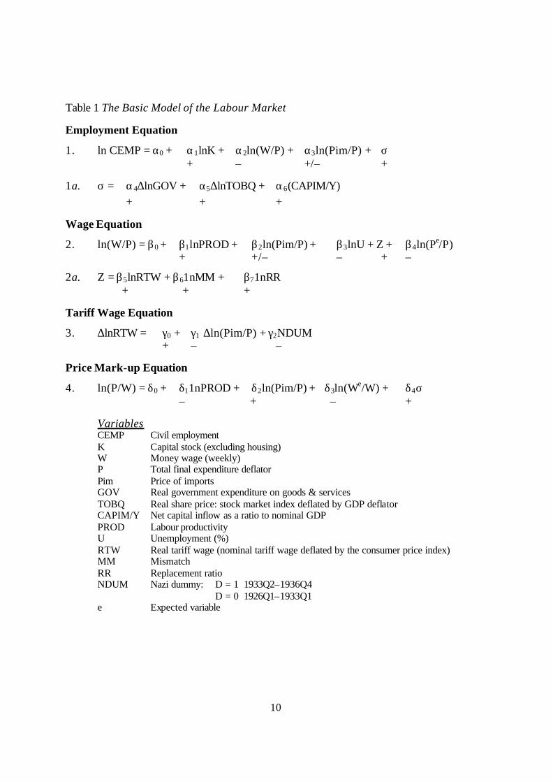
Table 1 The Basic Model of the Labour Market

Employment Equation

1. ln CEMP = α0 + α1lnK + α2ln(W/P) + α3ln(Pim/P) + σ + – +/– +

1a. σ = α4∆lnGOV + α5∆lnTOBQ + α6(CAPIM/Y) + + +

Wage Equation

2. ln(W/P) = β0 + β1lnPROD + β2ln(Pim/P) + β3lnU + Z + β4ln(Pe/P) + +/– – + –

2a. Z = β5lnRTW + β61nMM + β71nRR + + +

Tariff Wage Equation

3. ∆lnRTW = γ0 + γ1 ∆ln(Pim/P) + γ2NDUM + – –

Price Mark-up Equation

4. ln(P/W) = δ0 + δ11nPROD + δ2ln(Pim/P) + δ3ln(We/W) + δ4σ – + – +

Variables CEMP Civil employment K Capital stock (excluding housing) W Money wage (weekly) P Total final expenditure deflator Pim Price of imports GOV Real government expenditure on goods & services TOBQ Real share price: stock market index deflated by GDP deflator CAPIM/Y Net capital inflow as a ratio to nominal GDP PROD Labour productivity U Unemployment (%) RTW Real tariff wage (nominal tariff wage deflated by the consumer price index) MM Mismatch RR Replacement ratio NDUM Nazi dummy: D = 1 1933Q2–1936Q4 D = 0 1926Q1–1933Q1 e Expected variable

11

III. The Layard-Nickell Model of the Labour Market

The model of the labour market is derived from Layard and Nickell (1986) and Layard, Nickell and Jackman (1991). It consists of an employment equation, an equation for real wages and a price mark-up equation. The determination of the real wage and unemployment is the outcome of an interaction between the actions of wage setters, including trade unions and wage determining bodies, and the pricing policies of firms.

In the employment equation (Equation (1)), which, in common with the other equations of the model, is in log-linear form, employment is positively related to the capital stock and negatively to the real wage. The real wage is defined as the product wage which is relevant to the employment decisions of firms. The money wage is therefore deflated by the price of final output or TFE (total final expenditure) deflator. Employment also depends on the real price of imports that is the import price index deflated by the TFE deflator. The sign of the coefficient depends on whether imports are complementary or competitive with domestic output and employment. Imports of raw materials are likely to be complementary so that a rise in real import prices reduces employment. By contrast, imports of finished goods are likely to compete with domestic production so that the effect of a rise in real import prices on employment will be positive. The sign of the coefficient on real import prices is there-fore ambiguous, depending on the relative strength of these two factors.

Employment is affected by demand shocks, as well as the fundamental determinants, which have been discussed so far. These shocks are designated s and are shown in Equation (1a). A wide range of variables may be tested for inclusion as demand-side shocks. The variables on which we place most emphasis are the change in the real price of shares, de-fined as the share index deflated by the GDP deflator, the change in real government spend-ing on goods and services, and the ratio of capital inflow to nominal GDP. The first variable picks up the impact of the shifts in domestic business confidence. It uses the hypothesis of Ritschl (1999b) and Voth (2003), who both emphasize the importance of real share prices in the German recovery in the 1920s and their subsequent relapse from 1928. The change in real government expenditure allows the expansionary fiscal programme introduced under the Nazi regime to affect employment. The ratio of net capital i nflows to GDP is a measure of the impact of capital inflows on domestic activity and is unlogged as capital flows can be negative. The importance of capital flows has been emphasised by Ritchl (1998) and Bal-derston (1993).28 The demand variables enter in difference form because the structure of 28 Balderson (1993), pp. 212–14.

12

the model is bas ically neoclassical. The demand variables are grouped together as a single variable σ, where the weights attached to the individual components are estimated in the employment equation.

In the wage equation, Equation (2), the real wage, defined as the money wage deflated by the price of final output, is determined by both economic fundamentals, such as labour pro-ductivity and the unemployment, and the real tariff wage. The real wage is positively related to productivity as workers are offered higher real wages as labour productivity increases. Unemployment has a negative effect on the real wage, which reflects two distinct proc-esses. A higher level of employment strengthens the bargaining position of the labour force resulting in a higher real wage. In addition the wage setting policies of firms lead them to raise real wages to recruit more workers. This occurs on account of adverse selection in the labour market even in the absence of trade unions as shown in efficiency wage models of the labour market. Both collective bargaining and asymmetric information in the labour market can give rise to a positive relationship between employment and the real wage. Layard et al (1991).29 The real wage is also affected by mismatch and the replacement ratio. Mismatch occurs when unemployment is unequally distributed across industrial labour markets. There will be a higher degree of tightness in the aggregate labour market, when mismatch is greater at a given level of unemployment. The higher the replacement ratio, the greater is the incentive for workers to engage in search activity in labour markets. The real wage is therefore positively related to the replacement ratio in Equation (2). The real price of imports has a positive effect on the real wage as workers seek compensation for a rise in import prices by seeking a larger share of domestic output. An unexpected rise in prices reduces the real wage as workers are caught out by the price rise, while an unexpected fall in prices has the opposite effect.30 If money wages are sticky, there is more scope for un-foreseen price changes to affect the real wage. This effect is designated nominal inertia by Layard et al. (1991).31

There is a large literature which emphasizes the importance of the tariff wage in influ-encing labour market conditions under the Weimar Republic, which is reviewed by Balder-ston (1993)32 and noted by James (1986).33 We have taken account of this by including the

29 Layard et al.(1991) discuss wage bargaining pp. 83–143 and efficiency wages pp. 150–71. 30 This effect is picked up by Pe/P in the wage equation and similarly We/W in the price equation. 31 Layard et al.(1991), pp. 15–16. 32 Balderston (1993), pp. 18–48. 33 James (1986), pp. 204–13.

13

real tariff wage in the wage equation, where the nominal tariff wage is deflated by the con-sumer price index. We have then attempted to explain the determinants of the change in the tariff wage, which reflects a complex process of wage determination including compulsory state arbitration, as discussed in the literature.34 The real tariff wage, which enters into Equation (2), is explained by the tariff wage equation, Equation (3). Since this equation is in first differences a positive constant measures the upward pressure on the real wage due to the wage determining processes under the Weimar Republic. Under the Nazis the role of the tariff wage system was substantially altered, as noted by James (1986)35 and Bry (1960). It came to be used as a device to check the rise in the real wage by pegging the nominal tariff wage. This change of policy is modelled in our equation by a dummy variable for the Nazi era, which has an expected negative coefficient. The tariff wage equation also includes the change in the real price of imports prices, while the role of other economic variables, such as unemployment and mismatch, is also examined.

In the price equation, Equation (4), the price mark-up is negatively related to productiv-ity. This is part of the mechanism by which increased productivity is translated into higher real wages as wages rise more than prices. The mark-up is positively related to real import prices, since higher real import prices raise the gross margins of firms. Unexpected in-creases in money wages reduce the mark-up until firms have had time to adjust their pricing policies. There is scope for nominal inertia (We/W), due to price stickiness in response to unexpected changes in wages, to affect margins in the price equation. Finally demand pres-sure, s, using weights estimated from the employment equation, is included in the equation, since positive demand shocks may encourage firms to increase their mark-ups.

34 The process of wage determination is discussed in Balderston (1993), pp. 24–48. 35 James (1986), pp. 367–71.

14

It may be noted that the dependent variable for the price equation is the reciprocal of the

dependent variable for the wage equation. This arises because we are seeking to determine a point of intersection between a positively sloped wage equation and a horizontal or nega-tively sloped price mark-up equation.36 In the model equilibrium unemployment is the out-come of the price setting decisions of firms and wage determining processes in the labour market. The level of employment adjusts to bring the opposing forces into equilibrium.

CHARTS A

Chart A1: Percentage Unemployment

Chart A2: Civil Employment

Chart A3: Real Product Wage (W/P)

Chart A4: Real Tariff Wage (TW/CPI)

36 This equilibrium is shown in Fig. 1 (p. 32).

20,000

19,000

18,000

17,000

16,000

15,000

14,000

13,000 1925 1926 1927 1928 1929 1930 1931 1932 1933 1934 1935 1936 1937 1925 1926 1927 1928 1929 1930 1931 1932 1933 1934 1935 1936 1937

1925 1926 1927 1928 1929 1930 1931 1932 1933 1934 1935 1936 1937

.2

.15

.1

.05

.46

.45

.44

.43

.42

.41

.39

.38

.37

115

110

105

100

95

90

85

1925 1926 1927 1928 1929 1930 1931 1932 1933 1934 1935 1936 1937

15

Chart A5: Replacement Ratio

Chart A6: Real Price of Imports (IMPP/P)

Chart A7: Real Price of Shares (Share Price/Price GDP)

Chart A8: Capital Imports/GDP

.7

15

1925 1926 1927 1928 1929 1930 1931 1932 1933 1934 1935 1936 1937 1925 1926 1927 1928 1929 1930 1931 1932 1933 1934 1935 1936 1937

1925 1926 1927 1928 1929 1930 1931 1932 1933 1934 1935 1936 1937 1925 1926 1927 1928 1929 1930 1931 1932 1933 1934 1935 1936 1937

3.8

.75

3.7

.65

3.6

.55

3.5

.45

3.4

1.1

1

.9

.8

.7

.6

1.3

1.2

1.1

1

.9

.8

.7

.6

.5

15

10

5

0

–5

–10

16

Chart A9: Real Government Expenditure on Goods and Services

Chart A10: Annual Growth Rate of Real Tariff Rate

1925 1926 1927 1928 1929 1930 1931 1932 1933 1934 1935 1936 1937

1925 1926 1927 1928 1929 1930 1931 1932 1933 1934 1935 1936 1937

3000

2500

2000

1500

1000

12.5

10

7.5

5

2.5

0

–2.5

–5

17

IV. Variables and Methods

(a) The Main Variables of the Model

Before estimating the model we review the course of some of the principal variables, which are included in it. The quarterly data set covers the sample from the first quarter 1925 to the fourth quarter of 1936. The labour market series have been newly computed and details re-lating to their construction are set out in the Data Appendix.37 National income data have been drawn from Ritschl (1999a).

The initial set of variables relates to the labour market and the second set to the demand side variables, which could be included in the employment and price equations. Unemploy-ment shown in Chart A1 follows a gradually rising course until 1930, varying within a range of 5–10 per cent of the labour force. It then rises steeply, peaking at 25 per cent in 1932. From early in1932 there is a sustained decline, which reduces unemployment to the about the same level as at the beginning of the sample period. Civil employment, which is shown in Chart A2, follows a complementary course to the unemployment rate reaching a peak in 1928–9. The precise timing of the upper turning point of the Weimar boom is uncertain, since the various indicators peak at different times, as Borchardt (1991b)38 has noted. The severe decline in employment from 1929 to 1932 shows unambiguously the effect of the Great Depression, while the subsequent recovery shows up strongly in the employment data from 1932 to 1936. The model lays emphasis on the real product wage, defined as weekly earnings divided by the deflator for final expenditure. This series is plotted in Chart A3, which shows that the real wage increased throughout the boom of the late 1920s, as claimed by Borchardt (1991b),39 and continued to rise in the early stages of the slump. The real wage continued to grow in the downturn 1929–31 because the money wage was declining more slowly than the price of final output. From 1932 to 1934 the real wage fell as money wages were reduced more rapidly than prices, but after 1934 the real wage staged a mild re-covery. Chart A4 shows the real tariff or contract wage, defined as the tariff wage deflated by the consumer price index. The series increased sharply in the boom of the late 1920s, levelling off in 1930–31.There was a steep decline early in 1932, followed by a more grad- 37 The institutional background to the collection of the data used in this paper is discussed in Tooze (1999). 38 Borchardt (1991b), p. 172. 39 Borchardt (1991b), p. 183.

18

ual decline under the Nazi regime, when the real tariff wage was reduced by the deliberate policy of pegging the nominal tariff wage at a time of gently rising prices. The replacement ratio (the ratio of unemployment benefits to earnings) is plotted in Chart A5. The series rises strongly to 1927 and then falls steadily as benefits made available under the reformed unemployment scheme were progressively reduced as discussed in Balderston(1993).40 The real price of imports, defined as the price of imports deflated by the price of final output, is shown in Chart A6. It followed a downward trend, which gathered in pace during the depres-sion of 1929–32. This can be explained by the greater decline in the price of food and raw materials of which imports were largely composed compared to the price of final output.

We now turn to the demand-side variables which are included in s. These are the real price of shares, net capital inflow and real government expenditure on goods and services, The real price of shares or real Tobin Q, defined as the share index divided by the GDP de-flator, is shown in Chart A7. The real share price reached a peak in mid 1927, followed by a sharp decline to a low point in late 1931. There was then a sustained recovery to the end of 1936. The inflow of foreign capital, measured as a ratio to nominal GDP, reached a peak in 1928, before falling steeply to 1932, when there was a net outflow of capital, as shown in Chart A8. From 1932 until the end of the sample the balance was approximately zero. The last of the demand-side variables is real gove rnment expenditure on goods and services plotted in Chart A9. The series showed no clear trend before 1933, but followed a strong upward trend under the influence of Nazi policies from 1934 onwards.

Chart A10 shows the rate of change of the real tariff wage, which was positive under the Weimar Republic, prior to the severe measures taken by the Brüning government in late 1931. There were sharp reductions in 1932–3 and the decline continued under the Nazi pol-icy of pegging the nominal level of the tariff wage.

40 Balderston (1993), pp. 241–2.

19

(b) Econometric Methodology

Having set out a well-known model of the labour market, we estimate its parameters. The dynamic structure is determined using the general-to-specific methodology developed by Hendry and collaborators. The estimation is cons trained by a relatively short sample from 1925 Q4 to 1936 Q4. However a large amount of variability in the explanatory variables implies that the information contained in the sample is high so that the parameters of the model can be estimated effectively. This methodology has been proposed by Campos and Ericsson (1990) and has been applied to Australian interwar data in Dimsdale and Horse-wood (2002). A similar argument applies to our quarterly German data set.

Since a sample, which includes the Great Depression as well as a major change of politi-cal regime, is likely to be highly disturbed, we test the structural stability of our equations as far as a limited sample size permits. We remain within the methodology of structural modelling and do not use the VAR approach used by many researchers. Our aim is to esti-mate the parameters of a theoretical model and not to follow an atheoretical statistical pro-cedure such as a VAR.

20

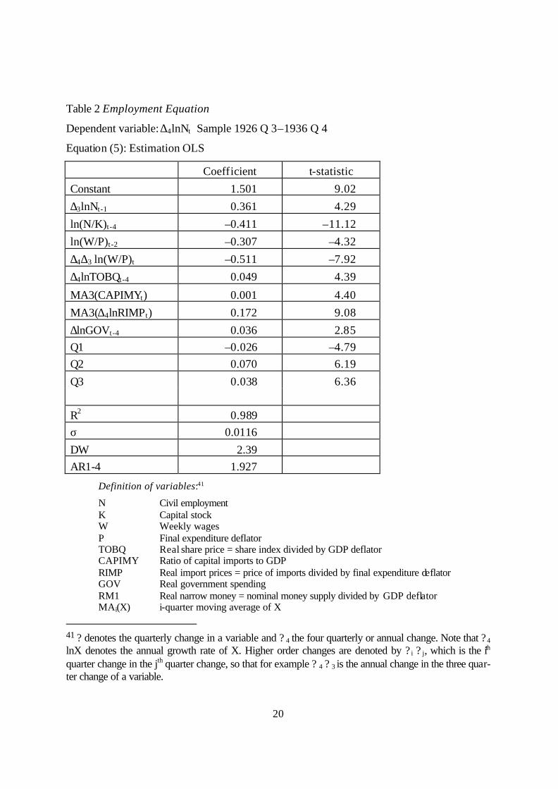
Table 2 Employment Equation

Dependent variable: ∆4lnNt Sample 1926 Q 3–1936 Q 4

Equation (5): Estimation OLS

Coefficient t-statistic Constant 1.501 9.02 ∆3lnNt -1 0.361 4.29 ln(N/K)t -4 –0.411 –11.12 ln(W/P)t -2 –0.307 –4.32 ∆4∆3 ln(W/P)t –0.511 –7.92 ∆4lnTOBQt -4 0.049 4.39

MA3(CAPIMYt) 0.001 4.40 MA3(∆4lnRIMPt) 0.172 9.08 ∆lnGOVt -4 0.036 2.85 Q1 –0.026 –4.79 Q2 0.070 6.19 Q3 0.038 6.36 R2 0.989 σ 0.0116

DW 2.39 AR1-4 1.927

Definition of variables:41

N Civil employment K Capital stock W Weekly wages P Final expenditure deflator TOBQ Real share price = share index divided by GDP deflator CAPIMY Ratio of capital imports to GDP RIMP Real import prices = price of imports divided by final expenditure deflator GOV Real government spending RM1 Real narrow money = nominal money supply divided by GDP deflator MAi(X) i-quarter moving average of X

41 ? denotes the quarterly change in a variable and ? 4 the four quarterly or annual change. Note that ? 4

lnX denotes the annual growth rate of X. Higher order changes are denoted by ? i ? j, which is the ith quarter change in the jth quarter change, so that for example ? 4 ? 3 is the annual change in the three quar-ter change of a variable.

21

Table 3 Wage Equation Dependent variable ∆4ln(W/P) t Sample 1927 Q1 – 1936 Q4 Equation (6): Estimation OLS

Coefficient t-stat Constant –1.994 –3.41 ln(W/P) t–4 –0.437 –3.61 ln(TW/Pcpi)t–4 0.328 2.74 lnPROD 0.095 7.73 D33Q1 0.036 3.73 lnRRt–4 0.059 2.22 ∆∆4lnRPIMPt 0.126 1.57 ∆4ln(TW/Pcpi)t 0.368 4.17 ∆2lnUt–2 –0.021 –2.48 lnUt–4 –0.046 –3.63 ∆4lnP t–4 –0.210 –3.27 Q1 0.003 0.69 Q2 –0.006 –1.62 Q3 0.002 0.43 R2 0.951 SE 0.0079 DW 2.140 AR(1–3) 1.316

Additional Variables

PROD 4 quarter moving average of hourly productivity TW/CPI Tariff wage deflated by consumer price index U Percentage unemployment RR Replacement ratio: unemployment benefits divided by average earnings

22

Table 4 Tariff Wage Equation Dependent variable ? ln (TW/CPI) t

Sample 1926 Q1 – 1936 Q4 : Estimation OLS Equation (7) Equation (8) Coefficient t-statistic Coefficient t-statistic Constant 0.007 2.06 NDUM –0.012 –3.42 –0.009 –2.71 D32q1 –0.050 –4.23 –0.047 –3.86 ∆2lnRPIMP –0.344 –4.36 –0.328 –3.97 Q1 0.001 0.25 0.006 1.41 Q2 0.007 1.47 0.015 3.74 Q3 –0.004 –0.88 0.003 0.69 R2 0.610 0.571 σ 0.011 0.012 DW 2.650 2.550

23

Table 5 Price Equation Dependent Variable ∆? 4 ln(P/W)t

Sample 1927 Q1–1936 Q4: Estimation OLS Equation (9) Coefficient t-stat Constant 0.068 2.62 ∆ln(P/W)t–4 –0.388 –3.89 ln(P/W) t–4 –0.085 –2.75 lnPROD –0.015 –1.75 ∆∆4lnWt –0.678 –7.58 ∆∆4lnWt–2 0.114 1.63 ∆2∆3lnRPIMPt–1 0.113 3.08 ∆2∆3lnRPIMPt–3 0.221 5.95 Q1 0.003 0.77 Q2 0.002 0.50 Q3 –0.002 –0.68 R2 0.841 SE 0.0077 DW 1.87 AR(1–3) 0.252

24

V. Empirical Results

(a) Employment Equation

The results of estimating the employment equation, Equation (5), are shown in Table 2. The equation is in equilibrium correction form and shows a short-run response of employment to the real wage with an elasticity of –0.307, which rises to –0.747 in the long run. This elasticity is comparable with that reported by Broadberry and Ritschl (1995). The real price of imports enters strongly in first differences of a moving average term. The annual growth rate in the real price of imports has a positive effect on employment, indicating that imports are on balance competitive with domestic output. There are also some dynamic effects in the real wage which are strongly significant. The variables which model demand shocks in the equation are the lagged annual change in the real price of shares (? 4ln TOBQ), the ratio of capital imports to GDP and lagged quarterly growth rate of real government spending on goods and services. Ritschl (1999b) argues that real share prices were an indicator of busi-ness confidence and had a powerful impact on investment. Since the series peaks in 1927, the implication is that the German downturn began well before the Wall Street crash. Voth (2003) puts forward a similar view on the role of the stock market.

Ritschl (1998) and Balderston (1993)42 have claimed that capital imports made a major contribution to the Weimar boom. The estimated equation points to the importance of both real share prices and capital inflows in explaining employment. It also finds a role for the proportional change in real government spending, which contributes to raising the demand for labour after 1932. Government spending follows an erratic course with large quarterly variations. The high variance of this variable could be reducing its significance in the em-ployment equation. Our estimates suggest that government expenditure had a positive im-pact on employment and was not fully offset through crowding out effects. To conclude, the employment equation yields well determined and plausible short and long-run elasticities for the real wage and confirms the significance of three sources of demand shocks.

(b) Wage Equation

The results of estimating the wage equation are shown in Table 3, where Equation (6) is in equilibrium-correction form. The real wage, defined as weekly earnings deflated by the

42 Balderston (1993), pp. 203–14.

25

price of final output, is positively related to productivity and the replacement ratio. Produc-tivity is measured hourly rather than quarterly to reduce cyclical effects. The real wage is negatively related to unemployment as expected. In additional the real wage was signifi-cantly affected by nominal inertia, represented by the annual rate of price inflation. This implies that that an increase in prices had a negative impact on the real wage as money wages responded with a lag to price changes. Similarly unexpected price declines tended to raise the real wage. This nominal inertia effect indicates a high degree of stickiness in money wages.Wage stickiness has been noted by Bry (1960)43 and could have been rein-forced by the wage determining arrangements under both the Weimar and Nazi regimes. Nominal inertia was also found to be important for interwar Britain by Dimsdale et al. (1989), where wages were chiefly determined by collective bargaining.

The real tariff wage is included in the wage equation to model the wage determining ar-rangements in interwar Germany. The importance of the tariff wage has been emphasized by writers, such as Balderston (1993), James (1986) and Borchardt (1991). The nominal tariff wage is deflated by the consumer price index, since the wage determining arrangements may be more focused on the real consumption wage than on the real product wage. The long-run coefficient of the real tariff wage in the wage equation is 0.650, indicating a pow-erful effect on real weekly earnings. This is not surprising in view of the high proportion of the labour force, which was subject to tariff wage agreements, as noted by Schacht (1931).44 In addition wages were influenced by more market related factors, such as the un-employment rate, productivity and the replacement ratio. These variables help to explain the gap between actual earnings and the minimum wages set by official bargaining procedures, which has been noted by James (1986).45 The wage equation serves to explain the wage drift, which James discusses. Finally there are several variables which enter the equation in dynamic form, such as the acceleration of real import prices and the change in the real tariff wage, while a dummy variable enters the equation for one quarter for data reasons. We in-cluded mismatch in the wage equation but did not find it to be significant.

43 Bry (1960), p. 158. 44 Schacht (1931), p. 198. 45 James (1986), p. 205.

26

(c) Tariff Wage Equation

Because of the need to include the real tariff wage in the wage equation, it is necessary to estimate an equation explaining this additional variable, which is not included in the basic Layard-Nickell model. We focus on explaining the change in the real tariff wage and the re-sults are shown in Table 4. Equation (7), which is our preferred equation, shows that the growth in the real tariff wage was negatively related to the second difference of real import prices. The negative sign indicates that the nominal tariff wage was not adjusted rapidly enough to compensate wage earners for changes in the real price of imports. The r emaining variables in the equation are measures of the effects of wage determining procedures, which were political in character. The positive constant indicates that there was upward pressure on the real tariff wage of 0.74 per cent per quarter under the Weimar government. Under the Nazis there was downward pressure on the real tariff wage of 0.46 per cent pe r quarter, which is calculated by adding the constant to the coefficient of the Nazi dummy. These re-sults accord with the accounts of the workings of the labour market under the Weimar Re-public, which emphasize the tendency for the outcome of wage determining processes to favour organized labour, James (1986)46 and Balderston (1993).47 It provides an explanation for Chart A10, which plots the quarterly rate of change of the real tariff wage. During the Weimar period there was upward pressure on the real tariff wage for reasons, which we have noted. By contrast under the Nazi regime the tariff wage was used as an instrument to keep down the real wage as shown in Chart A10. We also find a strongly significant dummy vari-able for first quarter 1932, which has a large negative coefficient. This may be interpreted as the consequence of the severe measures taken by the Brüning government to curb real wages in the depression under the Emergency Law of December 1931, discussed in Balder-ston (1993).48 It is notable that with the exception of import prices, economic variables, such as productivity growth and unemployment, did not affect the change in the tariff wage, which was apparently governed by non-economic factors. This result supports Borchardt’s contention that political factors were a major determinant of the course of tariff wages dur-ing the Weimar period. A similar argument applies to their Nazi successors, as noted by James (1986).49 46 James (1986), pp. 209–13. 47 Balderston (1993), pp. 43–3. 48 Balderston (1993), pp. 46–7. 49 James (1986), p. 368.

27

(d) The Price Equation

The estimation of the price-mark up leads to a relatively simple equation as shown in Equa-tion (9) in Table 5. It is estimated in equilibrium-correction form and indicates that the mark-up adjusts slowly, as shown by the small coefficient on the equilibrium correction term. The mark-up is negatively related to labour productivity, as expected on theoretical grounds. There is a significant dynamic term in the lagged annual change in wages. This im-plies nominal inertia, as unexpected wage changes affect the mark-up, which is reduced by an unexpected in increase in money wages. Real import prices enter in a dynamic form with a positive coefficient as higher import prices raise the mark-up of prices on wages. Most importantly, demand-side variables, which are included in s, do not enter the price equation, implying that the mark-up is not responsive to demand conditions. The prevalence of price fixing arrangements by cartels in interwar Germany, as noted by Petzina (1986),50 could help to explain this result. It also agrees with the results found by Dimsdale et al (1989) in estimating the price equation for interwar Britain, which in turn is supported the well-known study of the pricing behaviour of British firms by Hall and Hitch (1951). Price setting be-haviour in the two countries appears to have been similar in showing lack of response to demand conditions. Pricing setting therefore approximated to the normal cost hypothesis in which prices are set on the basis of a constant variable cost per unit plus a profit margin. This pricing procedure is examined by Layard and Nickell (1986) and is used extensively in Carlin and Soskice (1990). The terms for nominal ine rtia are of a higher order in the price equation than in the wage equation. This suggests a faster adjustment of prices in response to unexpected changes in wages than in wages in response to unexpected changes in prices. The marked difference in dynamic response to surprises in the wage and price equations helps to avert a potential problem of identification of the wage equation, which has been noted by Manning (1993).

(e) Parameter Constancy

In view of the change of regime during the sample period it is desirable to test for the sta-bility over time of the equations of the model. We report tests of parameter constancy over 8 quarters and 16 quarters for each of the structural equations of the model in Table 6. Each

50 Petzina (1986), p. 34.

28

equation shows parameter constancy over the forecast period. Constancy over the 16 quar-ter forecast implies that our equations are stable over the economic recovery and the change of political regime from Weimar to the Nazis. The equation for the change in the tariff wage Equation (7) is by definition not stable across a change of political regime and is therefore not tested. Table 6 Tests of Parameter Constancy Chow Break Tests 1935 Q1–1936 Q4 1933 Q1–1936 Q4 Employment Equation (5) F(8,21) 0.648 F(16,13) 1.050 Price Equation (9) F(8,21) 0.335 F(16,13) 0.830 Wage Equation (6) F(8,21) 1.495 F(16,13) 0.565

Actual and fitted values are shown for each of these equations in the charts below. Each equation tracks its dependent variable closely over a highly disturbed sample. Chart B4 shows that the quarterly change in the real tariff wage was generally positive under the Weimar Republic and negative under the Nazis. It can be seen that the impact of the Brüning measures of December 1931, modelled by a dummy variable for 1932 Q1, was powerful.

29

CHARTS B

Chart B1: Employment Equation Chart B2: Price Equation

1930 1935

Fitted D4LEWS

1930 1935

Fitted D4DLPW

.02

0

–.02

.1

0

–.1

30

Chart B3: Wage Equation

Chart B4: Tariff Wage Equation

Fitted DLRTWCPI

1925 1926 1927 1928 1929 1930 1931 1932 1933 1934 1935 1936 1937

.025

0

.02

1930 1935

Fitted D4LRWWR

.05

0

31

VI. The Analysis of Medium-Term Unemployment

The medium-term solution of the model for unemployment is obtained by solving out the lagged dependent variables in the Wage Equation (6) and the Price Equation (9) and setting the higher order dynamic terms equal to zero, but retaining all terms in nominal ine rtia. The long-run solutions for the wage and price equations are then combined to obtain the solu-tion for unemployment, as in Dimsdale et al . (1989). This is facilitated by the absence of s from the price equation. The Wage and Price Equations (6) and (9) become:

(10) ln (W/P) = –4.563 + 0.751 ln RTW + 0.217 ln PROD + 0.135 ln RR + 0.842 ? 4 ln RTW – 0.105 ln U – 0.481 ? 4 ln P

(11) ln (P/W) = 0.800 – 0.176 ln PROD – 7.976 ??4 ln W + 1.341 ??4 ln W

Eliminating the real wage by adding equations (10) and (11), we solve for unemployment to get equation (12):

(12) 0.105 ln U = –3.763 + 0.041 ln PROD + 0.751 ln RTW + 0.135 ln RR – 1.924 ? ln P + 3.368 ? ln RTW – 26.54 ? 2 ln W

For consistency annual differences ? 4 are expressed as quarterly differences ? with appro-priate adjustments of coefficients. The fundamental equation for unemployment is obtained by differencing Equation (12) and setting higher order terms equal to zero, so that ? 3 ln W = 0. The tariff wage equation Equation (7) is written:

(13) ? ln RTW = 0.0074 – 0.012 NDUM – 0.344 ? 2 ln RIMP

Differencing Equation (13) we note that ? 2 ln RTW = 0, since ? 3 ln RIMP= 0.

Taking the difference of Equation (12) and substituting for ? ln RTW from (13), gives the following equation, where ? ln U

UU∆

≈ :

(14) 0.105 UU/∆ = 0.041 ? ln PROD + 0.751 ? ln RTW + 0.135 ? ln RR – 1.924 ? 2 ln P

This equation is used for computing the determinants of medium term unemployment. It enables us to compute the impact of the explanatory variables on the change in unemploy-ment between selected benchmarks. These are selected to approximate to the downturn from 1928 to 1932 and the recovery from 1932 to 1936. The results of the calculations are shown in the table below.

32

Table 7 The Explanation of Unemployment

Effect of Change in Variable on Unemployment Rate (%) Tariff

Wage Replacement

Ratio Product-

ivity Price

Change Total Effect

1928–32 9.0 –5.0 0.3 6.7 11.0 1933–36 –10.0 2.0 0.8 –6.3 –13.5 Change in Unemployment Contribution of Variables % Predicted Actual Explanation

% Supply-

Side Demand-

Side 1928–32 11.0 17.4 63.2 39.1 60.9 1932–36 –13.5 –16.6 81.3 53.3 46.7 The upper part of Table 7 shows that in 1928–32 unemployment was raised by the increase in the real tariff wage, which was partly offset by the fall in the replacement ratio. The price change effect or nominal inertia raised unemployment due to a negative demand shock. In the recovery of 1932–6 the change in the real tariff wage reduced unemployment, while the change in the replacement ratio was less important than in the downturn. The change in prices reduced unemployment due to a positive demand shock.

The lower part of the table shows that the fundamental equation for unemployment, Equa-tion (14), explains 63 per cent of the rise in unemployment in the slump and 81 per cent in the upswing. The supply-side contribution is the sum of the effects on unemployment of changes in the real tariff wage, the replacement ratio and labour productivity. The impact of demand-side shocks is through nominal inertia. Both demand-side and supply-side variables are important in explaining changes in unemployment. The demand-side variable accounts for 60.9 per cent of the explained rise in unemployment 1928–32 and 46.7 per cent of the explained decline in unemployment 1932–6.

33

VII. Explaining Unemployment: A Diagrammatic Approach

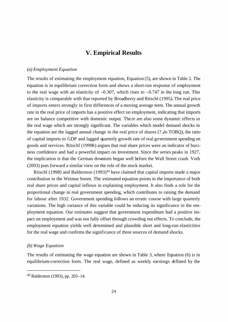
The explanation which the model provides of the course of unemployment can be illustrated by adapting diagrams used in Layard and Nickell (1986). In Figure 1 the labour demand function, D0, is negatively sloped with respect to the real wage, where employment is on the horizontal axis. It is subject to demand-side shocks which shift it to the right or to the left. The wage equation, W0, is positively sloped as a higher level of employment leads to greater tightness in the labour market. This strengthens the bargaining position of workers. It also prompts employers to offer higher wages to attract and motivate workers when there is asymmetric information in a competitive labour market. The wage function is shifted by a change in other variables in the wage equation, such as the replacement ratio and the real tariff wage. The price equation, P0, is horizontal, as the price-mark up does not vary with the level of employment as previously discussed. Equilibrium employment is shown at the in-tersection of all three relationships in Figure 1.

Under the Weimar Republic there was upward pressure on the wage function due to the processes for determining the real tariff wage, which shifted W0 to W1, so reducing the equilibrium level employment from E0 to E1. In the new equilibrium at E1 the real wage is unchanged as the price mark-up is horizontal. However during the adjustment process the real wage can rise as employment declines, as shown by the arrow in Figure 2. The impact of the depression was to shift the demand function D0 leftward to D1, so that the level of employment fell to E2. Thus the decline in employment was due partly to the shift to the left of the wage equation and partly to the leftward shift of the labour demand function. While the shift to the left of the wage function did not have a permanent effect on the real wage, there were dynamic effects shown by the arrow in Figure 2, which caused a temporary rise in the real wage.

During the contraction from 1928–32 both demand and supply-side factors were rai sing unemployment. The decline in the replacement ratio was tending to shift W0 to the right but this was more than offset by the upward pressure on the real wage due to the rise in the real tariff wage. Figure 2 shows that the decline in employment was due to both a fall in equilib-rium employment, largely on account of an increase in the real tariff wage, and a decline in employment relative to equilibrium employment, due to a negative demand shock.

34

Figure 1 W0

Real wage P D0 E0 Employment

Figure 2

W1

W0

Real wage P D0

D1 E2 E1 E0 Employment

35

Figure 3

W1

W2

Real wage P

D3

D2 E2 E3 E4 Employment During the recovery the contractionary forces were reversed. There was a positive demand shock shown in Figure 3 as shifting D2 to D3 and in addition the wage function shifted from W1 to W2, due to the reduction in the real tariff wage brought about by Nazi labour market policies. Equilibrium employment rose from E2 to E3, while actual employment rose fur-ther to E4 due to the expansionary fiscal policy of the Nazis. As the arrow in Figure 3 shows there was a temporary fall in the real wage during the process of adjustment. Thus demand and supply-side forces acted in a mutually reinforcing way in the both the recession and re-covery.

Two further points may be noted. First, while the initial period of expansion from 1926–8 is too short for our method of analysis, something can still be said about it. The wage curve was shifting to the left, as in Figure 2, due to upward pressure on the real tariff wage reducing equilibrium employment, while actual employment was rising due a positive de-mand shock on account of the Weimar boom. This implies that the economy was not in equilibrium. High employment could only be achieved by generating excess demand for la-bour, but this outcome was not sustainable, as Borchardt (1990)51 has argued. Secondly, the dummy variable for the first quarter of 1932 had a large negative effect on the real tariff wage. It models the consequences of the Emergency Decree of December 1931 in bringing 51 The unsustainability of the boom of the late 1920s is consistent with Borchardt’s view of the weak-nesses in the Weimar economy in the late 1920s, discussed in Borchardt (1990), pp. 126–37.

36

down the contractual wage. The real tariff wage was reduced with favourable effects on em-ployment as the reduction in the money wage was greater than the fall in prices. The Brün-ing wage cuts were followed by tentative policies for fiscal expansion under von Papen. Thus in its final stages the Weimar government was following policies which were condu-cive to recovery. These policies were continued by the Nazis through pegging the nominal tariff wage, while expanding aggregate demand. Policy was directed to both reducing the NAIRU and stimulating aggregate demand.

37

VIII. Relevance of the Model for German Economic History

The model which we have estimated is intended to be useful in shedding light a number of issues in German interwar economic history. The employment equation confirms that the demand for labour was sensitive to the real wage, which supports the results of ear-lier work by Broadberry and Ritschl (1995). However, in our model the real wage is en-dogenous and one must be cautious about concluding that excessive real wages were a cause of unemployment. Demand-side variables in the form of changes in real share prices, capital imports relative to GDP, and changes in government spending had a major effect on labour demand. The importance of real share prices in the employment equa-tion supports the contention of Ritschl (1999b) that this variable was indicative of busi-ness confidence. Voth (2003) finds a co-integrating relationship between investment and shares prices, which is consistent with the transmission mechanism between share prices and employment postulated in our model.52 The spike of real share prices in 1927–8 points to the contribution of domestic forces in precipitating the downturn be-fore the decline in exports and world trade in 1929. Net capital imports also play a ma-jor role, as argued by Ritschl (1998). Changes in government expenditure were found to be statistically significant and contributed to the recovery in the demand for labour un-der the Nazis from 1933 until the end of the sample period. This result suggests that a more expansionary fiscal policy could have raised employment in the slump, an issue which has been hotly disputed among German economic historians.53 Increased real im-port prices had a positive effect on employment, suggesting that home production was acting as a substitute for imports. The equation supports the view that the business cycle of the 1920s peaked in 1927–8 rather than 1929, since real share prices are more pow-erful than the effect of capital inflows. Hence Germany’s cycle of the late 1920s ap-pears to have an upper turning point generated by internal rather than external factors, as argued by Temin (1971) and Ritschl (1999b).

Turning to the two wage equations, we have modelled a two-tier model of the labour market in which both market forces and government intervention played a major role.

52 Voth (2001) reports a cointegrating relationship between the real interest rate and investment. We tried this variable in our employment equation and did not find it to be statistically significant unlike real share prices. Voth suggests that the real interest rate explains investment better than the real wage, which is a criticism of Borchardt’s wage pressure hypothesis. Our model is not subject to this criticism since the real wage enters into our labour demand equation and we do not model the im-pact of wage pressure on investment. In that respect our model differs from the process envisaged by Borchardt, which has been criticized by Voth. 53 See von Kruedener (1990), in particular the papers by Borchardt and Holtfrerich.

38

Balderston (1993)54 has proposed an informal model of this kind, which accords with our general approach. The most striking result which has emerged is that the market wage and the real tariff wage were determined by different factors. The market wage in-cludes economic fundamentals, such as productivity growth, the replacement ratio, real import prices and unemployment in addition to the real tariff wage. By contrast the real tariff wage was largely determined by incomes policy variables under both Weimar and Nazis. In that sense the tariff wage was a political wage. Real import prices are the only fundamental variables included in the tariff wage equation, since other economic vari-ables were found to be non-significant. The implication of this result is that the real tar-iff wage did not reflect economic fundamentals. It responded positively to upward pres-sure under the Weimar Republic. This effect was offset in the depression as a result of Brüning’s stringent wage reductions in December 1931. Under the Nazis the real tariff wage was reduced through the pegging of the nominal tariff wage, combined with a grad-ual rise in prices. Hence those writers who have argued that the determination of the tar-iff wage under the Weimar Republic was predominantly political are supported by our results. Borchardt (1990, 1991b)55 has advanced this view, whereas Balderston (1993)56 considers that the tariff wage reflected economic fundamentals through the bargaining processes. In view of the predominance of compulsory arbitration in major wage settle-ments, it is not surprising that political factors were dominant in resolving wage dis-putes. By contrast the market wage was responsive to economic variables, such as pro-ductivity, unemployment, mismatch and the replacement ratio. The difference between the market wage and the tariff wage was noted by James (1986)57 and our wage equation serves to support his view.

The wage equation shows strong evidence of nominal inertia, such that an unexpected increase in prices led to a reduction in the real wage. In the depression price declines had a positive effect on the real wage and this was an important factor contributing to a rising real wage in the early stages of the downturn. Nominal inertia was also found to be important in interwar Britain. However, in Germany there was a higher degree of wage stickiness in that real wages were affected by unexpected changes in the price level rather than in the rate of inflation. This form of wage inertia could be explained as a con-sequence of nominal wage contracts, which are noted by Balderston,58 and the pegging 54 Balderston (1993), Chap. 2. 55 Borchardt (1991b), pp. 181–2 and (1990), p. 146. Our results support his view that ‘The exis-tence of the wage drift does not refute the thesis of a forced increase [ in the real wage] in the 1920s brought about by trade unions and the system of public administration.’ 56 Balderston (1993), pp. 42–3. 57 James (1986), pp. 204–5. 58 Balderston (1983), pp. 24–6.

39

of the nominal tariff wage under the Nazis, as noted by both James59 and Bry.60 The rise in the market wage which occurred under the Nazis from 1934 is attributed to efficiency wage factors, which encouraged firms to bid for labour and to seek to provide incentives for the individual worker. This interpretation is consistent with the discussion of the la-bour market under the Nazis in Overy (1996), Mason (1966) and Siegal (1985). Siegal in particular describes the working of the labour market under the Nazis in which wages were set by employers to attract and motivate individual workers or small groups of workers. This could result in bonuses or incentive payments being paid which raised wages above the minimum rates specified in the tariff wage. Such behaviour is consistent with our finding of an upward movement in real wages under the Nazis and can be ex-plained by an efficiency wage model of the labour market.

59 James (1986), pp. 368–9. 60 Bry (1960).

40

IX Conclusion

The analysis of unemployment suggests that there was strong upward pressure on real wages under the Weimar Republic. This more than offset the effects of productivity growth on unemployment, which appear to have been negligible. During the Great De-pression there was a negative demand shock, which was communicated to the labour market by nominal inertia. On the supply-side the effect of the rising real tariff wage was partly offset by the decline in the replacement ratio. Thus both demand and supply-side influences reduced employment in the downturn. During the recovery of the 1930s nominal inertia played a major role in transmitting a large positive demand shock to the labour market. The impact of the Nazi policy of fixing the nominal tariff wage had a ma-jor effect on the real wage and on unemployment so that supply-side forces contributed to recovery. Unlike interwar Britain where demand shocks predominated in both slump and recovery, in Germany demand and supply-side forces reinforced each other in both phases of the cycle. This finding could help to explain both the severity of the downturn in Germany and the vigour of the recovery under the Nazis.

41

References

OFFICIAL PUBLICATIONS Statistisches Reichsamt (1927), Statistik des Deutschen Reichs, Band 402, Volks-,

Berufs- und Betriebszählung vom 16.Juni 1925, ‘Die berufliche und soziale Glied-erung der Bevölkerung des Deutschen Reichs’, Berlin.

Statistiches Reichsamt (1934), Statistik des Deutschen Reichs, Band 453, Volks-, Berufs- und Betriebszählung vom 16.Juni 1933, ‘Die berufliche und soziale Gliederung Der Bevölkerung des Deutschen Reichs’, Berlin.

Statistisches Reichamt (1924–1937), Wirtschaft und Statistisk, Berlin. Institut für Konjunkturforschung (1933, 1936), Konjunkturstatisches Handbuch, Ber-

lin. Institut für Konjunkturforschung (1933–7), Vierteljahreshefte zur Konjunkturfor-

schung, Berlin. Institut für Konjunkturforschung (1933–7), Wochenbericht zur Konjunkturforschung,

Berlin. Reichsarbeitsministerium (1924–37), Reichsarbeitsblatt, Berlin. ARTICLES AND BOOKS Balderston, T. (1977) ‘The German business cycle in the 1920s: A comment’, Economic

History Review 30, 159–61. Balderston, T. (1982), ‘The origins of economic instability in Germany 1924–1930:

market forces versus economic policy’, Vierteljahrschnift für Sozial- und Wirtschaftgeschichte, 69, 488–514.

Balderston, T. (1993), The Origins and Cause of the German Economic Crisis, 1923–1932 (Berlin).

Balderston, T. (2002), Economics and Politics in the Weimar Republic (Cambridge). Borchardt, K. (1991a), ‘Constraints and room for manoeuvre in the Great Depression of

the early Thirties: towards a revision of the received historical picture’, in K. Bor-chardt (ed.), Perspectives on Modern German Economic History and Policy (Cam-bridge; German orig. 1980).

Borchardt, K. (1991b), ‘The economic causes of the collapse of the Weimar Republic’, in K. Borchardt (ed.), Perspectives on Modern German Economic History (Cam-bridge; German orig. 1979).

Borchardt, K. (1990), ‘A decade of debate about Brüning’s economic policy’, in J. von Kruedener (ed.), Economic Crisis and Political Collapse: The Weimar Republic 1924–1933 (Oxford).

Borchardt, K. and Ritschl, A. (1992), ‘Could Brüning have done it? A Keynesian model of inter-war Germany, 1925–1938’, European Economic Review 36, 695–701.

42

Bowen, W.G. and Finegan, T.A. (1969). The Economics of Labor Force Participation (Princeton)

Bracher, K.D. (1954), Die Auflösung der Weimarer Republik. Zum Problem des Machtverfalls in der Demokratie (Villingen).

Broadberry, S.N. and Ritschl, A. (1995) ‘Real wages, productivity and unemployment in Britain and Germany during the 1920s’, Explorations in Economic History, 32, 327–49.

Brüning, H. (1970), Memoiren 1918–1934 (Stuttgart). Bry, G. (1960), Wages in Germany 1871–1945 (Princeton). Campos, J. and Ericsson, N.R. (1990), ‘Economic Modeling of Consumers’ Expenditure

in Venezuela’, Board of Governors of the Federal Reserve System, Washington, DC. Carlin, W. and Soskice, D. (1990), Macroeconomics and the Wage Bargain: A Modern

Approach to Employment, Inflation and the Exchange Rate (Oxford). Corbett, D. J. (1991), Unemployment in Interwar Germany, 1924–1938, unpublished

thesis, Harvard University. Dimsdale, N.H., Nickell, S.J. and Horsewood, N. (1989), ‘Real wages and unemploy-

ment in Britain during the 1930s’, Economic Journal, 99, 271–92. Dimsdale, N.H. and Horsewood, N. (2002), ‘The causes of unemployment in interwar

Australia’, Economic Record, 78, 388–405. Eichengreen, B. (1992), Golden Fetters: The Gold Standard and the Great Depres-

sion, 1919–1939 (Oxford). Eichengreen, B. (1994), ‘Perspectives on the Borchardt debate’, in C. Buchheim, M.

Hutter and H. James (eds.), Zerrissene Zwischenkreigszeit (Baden Baden), 177–203.

Erbe, R. (1958), Die Nationalsozialistische Wirtftshaftspolitik 1933–1939 im Lichte der modernen Theorie. (Zurich).

Eschenburg, T. (1984), Die Republik von Weimar. Beiträge zur Geschichte einer Im-provisierten Demokratie (Munich and Zurich).

Falkus, M.E. (1975), ‘The German business cycle in the 1920s’, Economic History Re-view, 28, 451–65.

Falter, J., Lindenberger, T. and Schumann, S. (1986), Wahlen und Abstimmungen in der WeimarerRepublik (Munich).

Galenson, W. and Zellner, A. (1957), ‘International Comparison of Unemployment’, in NBER, The Measurement and Behaviour of Unemployment (Princeton).

Hachtmann, R. (1988), ‘Lebenshaltungskosten und Reallöhne während des Dritten Reichs’, Vierteljahrschrift für Sozial- und Wirtschaftsgeschichte, 75, 32–73.

Hall, R.L. and Hitch, C.J. (1951), ‘Price Theory and Business Behaviour’, in Oxford Studies in the Price Mechanism, T. Wilson and P.W.S. Andrews (eds). (Oxford).

43

Hamann, H. (1945), ‘Das Lohnproblem im Landbau’, Weltwirtschaftliches Archiv 61, 193–213.

Heiber, H. (1966), Die Republik von Weimar (Munich). Helbich, W. J.(1962), Reparationen in Der Ära Brüning. Zur Bedeutung des Young

Plans für die Deutsche Politik (Berlin). Hoffman, W.G., Grumbach, F. and Hesse, H. (1965), Das Wachstum der deutschen

Wirtschaft der Mitte des 19 Jahrhunderts (Berlin). Holtfrerich, C.-L. (1984), ‘Zu hohe Löhne in der Weimarer Republik? Bemerkungen zur

Borchardt These’, Geschichte und Gesellschaft, 10, 122–41. Holtfrerich, C.-L. (1990), ‘Was the policy of deflation in Germany unavoidable?’, in

J. von Kruedener (ed.), Economic Crisis and Political Collapse: The Weimar Re-public 1924–1933 (Oxford).

James, H. (1986), The German Slump: Politics and Economics 1924–1935 (Oxford). James, H. (1990), ‘Economic Reasons for the Collapse of the Weimar Republic’, in

I. Kershaw (ed.), Weimar: Why did German Democracy Fail? (London). Layard, P.R.G., and Nickell, S.J. (1986), ‘Unemployment in Britain’, in C. Bean,

R. Layard and S. Nickell (eds.), The Rise in Unemployment (Oxford), 121–69. Layard, P.R.G., Nickell, S.J. and Jackman, R. (1991), Unemployment: Macroeconomic

Performance and the Labour Market (Oxford). Livchen, R. (1944), ‘Net Wages and Real Wages in Germany’, International Labour

Review, 40, 65–72. Lölhöffel, M. von (1974), ‘Zeitreihen für den Arbeitsmarkt. Lohnsatz, Beschäftigungs-

fälle, Arbeitskosten und Arbeitsstunden’, Ifo Studien, 20, 33–150. Manning, A. (1993). ‘Wage bargaining and the Phillips curve: the identification and

specification of aggregate wage equations’, Economic Journal 103, 98–118. Mason, T.W.(1966) ‘Labour in the Third Reich, 1933–1939’, Past & Present, 12, 112–

41. Müller, H.(1953), Nivellierung und Differenzierung der Arbeitseinkommen in

Deutschland seit 1925 (Berlin). Overy, R.J. (1996), The Nazi Economic Recovery 1932–38, 2nd ed. (London). Peukert, D.(1988), ‘The Weimar Republic Old and New Perspectives’, German History,

6, 133–44. Petzina, D. (1986), ‘The extent and cause of unemployment in the Weimar Republic’, in

P.D. Stachara (ed.), Unemployment in the Great Depression in Weimar German (London).

Reulecke, J. (1974), ‘Veränderungen des Arbeitskräftepotentials im Deutschen Reich 1900–1933’, in H. Mommsen, D. Petzina, and B. Weisbrod (eds.), Industrielles Sys-tem und Politische Entwicklung in der Weimarer Republik (Dusseldorf).

44

Riel, A. van and Shram, A. (1993), ‘Weimar economic decline, Nazi economic recovery and the stabilization of political dictatorship’, Journal of Economic History, 53, 71–105.

Ritschl, A. (1998), ‘Reparations transfers, the Borchardt hypothesis and the Great De-pression in Germany, 1929–32: A guided tour for hard-headed Keynesians’, Euro-pean Review of Economic History, 2, 49–72.

Ritschl, A. (1990), ‘Zu hohe Löhne in der Weimarer Republik? Eine Auseinandersetzung mit Holfrerichs Berechnungen zur Lohnposition der Arbeiterschaft 1925–1932’, Geschichte und Gesellschaft, 16, 375–402.

Ritschl, A. (1999a), Deutschlands Krise und Konjunktur, 1924–1934: Binnenkon-junktur, Auslands-verschuldung und Reparationsproblem zwischen Dawes-Plan und Transfersperre (Berlin).

Ritschl, A. (1999b), ‘Peter Temin on the onset of the Great Depression in Germany: A Reappraisal’, mimeo.

Ritschl, A. (1998), ‘Reparation transfers, the Borchardt hypothesis and the Great De-pression in Germany, 1929–32: A guided tour for hard-headed Keynesians’, Euro-pean Review of Economic History, 2, 49–72.

Sanmann, H. (1965), ‘Daten und Alternativen der Deutschen Wirtschafts- und Fi-nanzpolitik in der Ära Brüning’, Hamburger Jahrbuch für Wirtschafts- und Gesell-schaftspolitik, 10, 109–40.

Schacht, H. (1931), The End of Reparations: The Economic Consequences of the World War (ed.), G. Glasgow (London).

Schulze, H. (1942), Die Entwicklung der Landarbeiterlöhne, ihrer Kaufkraft und das Verhältnis zu den Industriearbeitlöhne. Dissertation, Institut für Agrarwesen und Agrarpolitik, Berlin.

Schmidt, C.T. (1934), German Business Cycles 1924–1933 (New York). Siegel, T. (1985), ‘Wage policy in the Third Reich’, Politics and Society, 14,

1–41. Sommariva, A. and Tullio, G. (1987), German Macroeconomic History, 1880–1979

(London). Stögbauer, C. (2001), ‘The radicalization of the German electorate: swinging to the right

and to the left in the twilight of the Weimar Republic’, European Review of Eco-nomic History, 5, 251–80.

Temin, P. (1971), ‘The beginning of the Depression in Germany’, Economic History Re-view, 24, 240–8.

Tooze, J.A. (1999) ‘Weimar’s statistical economics: Ernst Wagemann, The Reich’s Sta-tistical Office and The Institute for Business-Cycle Research’, Economic History Review, 24, 523–43.

45

Voth, H.-J. (1995), ‘Did high wages or high interest rates bring down the Weimar Re-public? A cointegration model of investment in Germany, 1925–1930’, Journal of Economic History, 55, 801–21.

Voth, H.-J. (2003), ‘With a bang, not a whimper: pricking Germany’s “stock market bub-ble” in 1927 and the slide into depression’, Journal of Economic History, 63, 65–99.

Weigart, O. (1934), Administration of Placement and Unemployment Insurance in Germany (New York).

Weisbrod, B. (1985), ‘Die Befreiung von den “Tarffesseln”. Deflationspolitik als Krisenstategie der Unternehmer in der Ära Brüning’, Geschichte und Gesellschaft, 11, 295–325.

Wermel, M. and Urban, R. (1949), ‘Arbeitslosenfürsorge und Arbeitlosenversicherung in Deutschland’, Neue Soziale Praxis, Heft 6/I–III.

46

Data Appendix Employment

The working population is taken from the occupational censuses (Berufszahlungen) held in 1925 and 1933. The IfK Handbuch reports monthly statistics on dependent employ-ment based on Health Insurance membership. Quarterly employment is obtained in the following way: the 1925 census data on employment was corrected for unemployment using information provided by labour exchanges. Published Health Insurance data are distorted by increasing coverage during the 1920s as noted by Ritschl (1991a). How-ever, changes between years are shown with a fixed coverage. From this data an index can be constructed which is linked to the absolute level of employment in later years, where the published data are no longer affected by changes in coverage. To adjust for the incomplete coverage of mandatory insurance, insurance data on dependent employment were raised to the level of the total for the census categories for Arbeiter, Angestellte and Beamte. Health Insurance data covered 92.3% of census wage and salary employ-ment in June 1925 and June 1933. Estimates for self employment and domestic servants were added by interpolating the census statistics using Health Insurance data.

Unemployment

The most appropriate measure of unemployment is the number of persons registered at labour exchanges who are seeking work, as pointed out by Balderston (1993). This is preferable to the adjusted trade union unemployment used by Galenson and Zellner (1957) and Peukert (1988). Data on labour markets, including statistics on job search, are given in the Reichsarbeitsblatt and Wirtschaft und Statistik but the number of un-employed registered at labour exchanges is not available until August 1929. In later years job search figures were corrected by the IfK to derive monthly unemployment fig-ures back to January 1924.

In the later Weimar years there is a problem of defining the level of unemployment. There is a difference between the total numbers registered as seeking work on 16 June 1933, the day of the occupational census, and those describing themselves as Erwerb-slos in the census returns. The difference is about 800,000 persons. It is treated here as evidence those who declared themselves to be without a job in the census but did not register at a labour exchange were discouraged workers or members of agricultural families not actively seeking work. This approach follows Balderston (1993) and Wei-gart (1934).

Consumer Prices

The official consumer price index is from Statische Jahrbuch für das Deutsche Reich, Wirtschaft und Statistik and the supplement to the IfK’s Wochenbericht. The expendi-ture weights used in combining the components of the index were based on a survey of household budgets made in 1907 adjusted to 1913–14 relative prices. The weights were

47

unchanged until autumn 1934, when a new set of weights was introduced based on a sur-vey of household budgets in 1927/8 with an increase in the number of items included from 67 to 116. The index was criticized by Livichen (1944) and Hachtmann (1988) for using inappropriate weights. Several inquiries were also made into household expendi-ture patterns between 1927/8 and 1937. Weights from these surveys were used in calcu-lating a revised consumer price index, but the difference with the official index was minimal. The official index has therefore been retained.

Import Prices

From January 1928 import prices are implicit in the monthly statements of nominal val-ues and their respective volumes in 1928 Reichmarks are given in the Konjunktursta-tistische Handbuch (1936), which continued in the Vierteljahresheft zur Konjunktur-forschung. For the period before 1928 both the 1933 and 1936 Handbuch report nomi-nal values for imports. Annual import and export values and volumes were obtained from Ritschl (1999a). The implicit annual import price series was interpolated using the Reichamt’s monthly wholesale price index. The resulting series was then linked to the previous series from 1928.

TFE Deflator

This is a combination of the import price series and the GDP deflator with weights given by the current value of imports and nominal GDP. Imports at current prices are from the Konjunkturstatistisches Handbuch and from the Wochenbericht towards the end of the period. Nominal GDP is from Ritschl(1999a).

Tariff wages

A weighted average of tariff wages for 15 branches of industry, postal services and rail-ways for years between 1925 and 1931is available in Reichsarbeitblatt II 1931 and Wirtschaft und Statistik 1931.61 From June 1931 the data is reported monthly and in detail. This can be linked to a series of revised data provided by the Reichamt. For the months up to December 1933 the series is available in Bry (1960) and it is continued in the A section supplements of Ifk’s Wochenbericht. The data include wages for skilled, semi-skilled and unskilled male workers and female workers. Employment weights are given in the Vierteljahershefte zur Statistik des Deutschen Reichs (1931) which en-ables an aggregate index to be computed.

Weekly Earnings

There is a lack of information on actual wages paid over a wide range of industries. Data is however available for average economy-wide wages and salaries. The basis for calcu-lation is the quarterly data on aggregate wage and salary sums which are given from 1925.1 to 1935.3 in the Konjunktur Statistische Handbuch (1936) and later estimates

61 Tariff wage data are assessed by Schulze (1942), Hamann (1945) and Müller (1970).

48

in the statistical supplements of the Wochenbericht (B section). Average earnings are divided by the index of wage and salary employment previously constructed. Weekly earnings are obtained by multiplying wage and salary employment by the 13 weeks in each quarter. In this we are using the method employed by von Lölhöffel (1974) in com-puting average annual earnings.

Productivity

This is defined as the ratio between real GDP and employment with the latter adjusted for hours worked per day and days per quarter. Data on the average number of hours worked per day and number of days worked each month in all industrial branches are given in the Konjunkturstatistisches Handbuch (1936) and in supplements to the Wochenbericht.

Replacement Ratio

The replacement rate is defined as the ratio of benefits paid for the initial period of un-employment to the average claimant to average earnings after taxes and social security deductions.

The first stage is the calculation of the tax wedge by adjusting wages for tax, social security payments and other deductions. Changes in taxes and social security contribu-tions are set out in Hachtman (1988) and calculations of deductions have been made by Livchen (1944), Bry (1960) and Corbett (1991). The main source is the special edition of Einzelschriften zur Statistik des Deutschen Reichs covering the period 1926–36 and detailed changes in premiums and taxes in the Reicharbeitsblatt and the Reichsgezets-blatt. From these sources a precise chronology of changes in deductions was con-structed to provide quarterly estimates. These deductions were applied to the series for average earnings. Average income and payroll taxes were calculated for a family of four persons with one earner receiving an average wage. Deductions are made for income tax, unemployment insurance, health insurance, disability insurance, poll tax and pensions. Nazi deductions, although nominally voluntary, are treated as being compulsory and in-clude contributions to the German Labour Front (DAF) and the Winter Relief Fund (Winterwerk).

The second stage is the calculation of benefits for the unemployed. Unemployment benefits are derived from monthly amounts spent on unemployment insurance and the corresponding number of claimants from Reichsarbeitsblatt II (nichtamtlicher Teil) and its statistical appendix. Unemployment data relate to the end of each month and the pool of unemployed is subject to inflows and outflows during each month. In making an esti-mate of the effective number of claimants it is assumed that inflows and outflows occur linearly over each month. The numbers leaving or entering the pool of unemployed are weighted by the number of days spent in unemployment to yield a measure of full dura-tion unemployed at the end of the month, which is added to the previous end of month total. Since transfer payments are monthly, wages are on the same basis for calculating

49

the replacement ratio. The maximum period for which benefits were paid at the initial rate varied, but a 26-week period defines the most relevant time span. The average com-pleted spell duration rises from a month in 1928 to a maximum of between 7 and 8 months in 1933, Corbett (1991). The inclusion of the subsequent lower Emergency Re-lief payments would make the calculated replacement rate dependent on the average du-ration of unemployment.

Mismatch

Mismatch is measured as the variance of unemployment across industries. It is repre-sented by the square of the coefficient of variation of unemployment by industry, fol-lowing Layard et al. (1991). Registered unemployment by industry is available from Au-gust 1929 for 28 categories of labour, including white collar workers. Before this date, the only data by industry, which is available is on job search. Data from which employed job seekers have been removed is provided by the IfK at an aggregate level. The ratio of unemployed job seekers to unemployed is about 80% in aggregate. This ratio of the two aggregate time series can be used to adjust the job search data to generate a series for unemployment disaggregated by industry. These are then related to the size of the blue collar labour force by industry according to the 1933 census. In doing so, the separate category of unemployment among white collar workers was deducted in proportion to the distribution of employment by sector by type of work (whether blue or white collar) in the 1933 census.

Other variables

GDP at constant prices, nominal GDP, business capital stock, government expenditure on goods and services, Tobin’s Q and net capital imports from Ritschl (1999a).

[Continued from inside front cover]

19 Liam Brunt, Nature or Nurture? Explaining English Wheat Yields in the Agricultural Revo-lution (Oct. 1997)

20 Paul A. David, Path Dependence and the Quest for Historical Economics: One More Cho-rus of the Ballad of QWERTY (Nov. 1997)

21 Hans-Joachim Voth, Time and Work in Eighteenth-Century London (Dec. 1997)

22 Tim Leunig, New Answers to Old Questions: Transport Costs and The Slow Adoption of Ring Spinning in Lancashire (Feb. 1998)

23 Paul A. David, From Keeping ‘Nature’s Secrets’ to the Institutionalization of ‘Open Sci-ence’ (July 2001)

24 Federico Varese and Meir Yaish, Altruism: The Importance of Being Asked. The Rescue of Jews in Nazi Europe (May 1998)

25 Avner Offer, Epidemics of Abundance: Overeating and Slimming in the USA and Britain since the 1950s (Nov. 1998)

26 David Stead, An Arduous and Unprofitable Undertaking: The Enclosure of Stanton Har-court, Oxfordshire (November 1998)

27 Oliver Grant, The Diffusion of the Herringbone Parlour: A Case Study in the History of Agricultural Technology (December 1998)

28 Antonia Taddei, London Clubs in the Late Nineteenth Century (April 1999)

29 Liam Brunt, Estimating English Wheat Production in the Industrial Revolution (June 1999)

30 Matthew Braham, Volunteers for Development: A Test of the Post-Materialism Hypothesis in Britain, c.1965–1987 (June 1999)

31 Paul A. David and Gavin Wright, General Purpose Technologies and Surges in Productiv-ity: Historical Reflections on the Future of the ICT Revolution (September 1999)

32 Liam Brunt, An Arbitrage Model of Crop Rotation (September 1999)

33 Paul A. David and Gavin Wright, Early Twentieth Century Productivity Growth Dynamics: An Inquiry into the Economic History of ‘Our Ignorance’ (October 1999)

34 Avner Offer, Economic Welfare Measurements and Human Well-Being (January 2000). Rev. version, March 2000.

35 Liam Brunt, ‘Where there’s Muck, There’s Brass’. The Market for Manure in the Indus-trial Revolution (February 2000).

36 Alasdair Crockett, Variations in Churchgoing Rates in England in 1851: Supply-Side Defi-ciency or Demand-Led Decline? (August 2000).

37 Martin West, State Intervention in English Education, 1833–1891: A Public Goods and Agency Approach (October 2000).

38 George Speight, Who Bought the Inter-War Semi? The Socio-Economic Characteristics of New-House Buyers in the 1930s (December 2000)

39 Peter Temin, A Market Economy in the Early Roman Empire (March 2001)

40 Michael Biggs, Positive Feedback in Collective Mobilization: The American Strike Wave of 1886 (April 2001)

41 Charles H. Feinstein and Mark Thomas, A Plea for Errors (July 2001)

42 Walter Eltis, Lord Overstone and the Establishment of British Nineteenth-Century Mone-tary Orthodoxy (December 2001)

43 A. B. Atkinson, Top Incomes in the United Kingdom over the Twentieth Century (February 2002)

44 Avner Offer, Why has the Public Sector Grown so Large in Market Societies? The Politi-cal Economy of Prudence in the UK, c.1870–2000 (March 2002)

45 Natàlia Mora Sitjà, Labour and Wages in Pre-Industrial Catalonia (May 2002)

46 Elaine S. Tan, ‘The Bull is Half the Herd’: Property Rights and Enclosures in England, 1750–1850 (June 2002)

47 Oliver Wavell Grant, Productivity in German Agriculture: Estimates of Agricultural Produc-tivity from Regional Accounts for 21 German Regions: 1880/4, 1893/7 and 1905/9 (Au-gust 2002)

48 Oliver Wavell Grant, Does Industrialization Push up Inequality? New Evidence on the Kuznets Cure from Nineteenth-Century Prussian Tax Statistics (September 2002)

49 Alexandre Debs, The Source of Walras’s Idealist Bias: A Review of Koppl’s Solution to the Walras Paradox (January 2003)

50 Robert Dryburgh, ‘Individual, Illegal, and Unjust Purposes’: Overseers, Incentives, and the Old Poor Law in Bolton, 1820–1837 (March 2003)

51 David R. Stead, Risk and Risk Management in English Agriculture, c.1750–1850 (October 2003)

52. Pablo Astorga, Ame R. Bergés, and Valpy FitzGerald, Productivity Growth in Latin America during the Twentieth Century (December 2003)

53. Teresa da Silva Lopes, Evolution of Corporate Governance in Global Industries: The Case of Multinationals in Alcoholic Beverages (February 2004)

54 Pablo Astorga, Ame R. Bergés, and Valpy FitzGerald, The Standard of Living in Latin Amer-ica during the Twentieth Century (March 2004)

55 Regina Grafe, Popish Habits vs. Nutritional Need: Fasting and Fish Consumption in Iberia in the Early Modern Period (May 2004)

56 Nicholas Dimsdale: Unemployment and Real Wages in Weimar Germany (October 2004)

University of Oxford Discussion Papers in

Economic and Social History

are edited by:

Robert Allen Nuffield College, Oxford, OX1 1NF

Jane Humphries

All Souls College, Oxford, OX1 4AL

Siobhan McAndrew Nuffield College, Oxford, OX1 1NF

Avner Offer

All Souls College, Oxford, OX1 4AL

Papers may be downloaded from http://www.nuff.ox.ac.uk/Economics/History/