Department of Economics University of Southampton Southampton SO17 1BJ UK

Discussion Papers in Economics and Econometrics 2000

This paper is available on our website http://www/soton.ac.uk/~econweb/dp/dp00.html

Creative Destruction and Policiesin a Vintage Model of Endogenous Growth

Xavier Mateos-PlanasDepartment of EconomicsUniversity of Southampton

High…eld SO17 1BJSouthampton, UK

E-Mail: fxmp@soton.ac.uk

Version 2.110 November 2000

Abstract

This paper extends a model of endogenous growth through the introduction of aproductivity-augmenting component of knowledge that makes new technologies moreproductive than older vintages. The paper characterizes equilibrium transitional andlong-run properties for the economy. The phenomenon of creative destruction, orobsolescence, of technologies underlies the growth process. In this set up, the growth-e¤ects of various policies are analyzed. These policies include vintage-speci…c subsi-dies to …rms that produce …nal output, a general lump-sum tax on …nal output …rms,and openness to trade with a less developed country. The results show the existenceof growth e¤ects that are absent in previous literature.

1

1 Introduction

Technological change and innovation involve the emergence of new products and technolo-

gies, along with the gradual displacement of old ones. Economic history provides many ex-

amples of this phenomenon that have been documented in, for example, Rosenberg (1982)

and Mokyr (1990). That the process of replacement of new goods and sectors for older ones

is a substantive ingredient of modern economic growth is not a new idea, having been …rst

expressed in Schumpeter (1942)’s celebrated notion of creative destruction. In this view,

economic progress is the cause as well as the consequence of the rise and decline of sectors

and …rms.

If innovation and obsolescence interact, then factors and policies that in‡uence the

intensity and pattern of the obsolescence process will have implications for economic growth.

For example, policies in the form of taxes and subsidies that are selective in terms of the

vintages targeted might alter the relative position of old and new sectors. In fact, policies

are often selective. A case in place is when declining pro…ts and employment in mature

sectors prompt a protective government response. Similarly, but with an opposite slant,

infant-industry policies seek to prop up new emergent economic activities.1

The aim of this paper is to investigate the implications of a variety of policy interven-

tions for growth and welfare in the presence of technological obsolescence. To that end,

two objectives will be pursued. The …rst is to gain an understanding of the features of an

economy undergoing the process of gradual replacement of new for old …rms and sectors.

This allows to take up the second objective which is to analyze, in this context, the conse-

quences of selective taxation and subsidies, lump-sun taxes, and openness to trade for the

process of growth.

This investigation is based on the analysis of a model that extends previous work on

endogenous growth theory. The model borrows its basic structure from Grossman and

Helpman (1991) so that privately conducted R&D is the engine of growth. The paper

1Selective policies have been documented in the fast-developing experiences of Korea, Singapore andTaiwan [see Young (1992) and Westphal (1990)]. In these cases, the government has been involved inchanneling credit to selected industries. Sector-speci…c policies are, in fact, a central theme in developmentpolicy [see, for example Kruger (1990), and Pack and Westphal (1986)]. Nonetheless, casual observationindicates that in developed countries targeted industrial policies are not rare either. There is the importantliterature on the political economy of trade protection that seeks to understand precisely why governmentsdeploy policies in favor of particular economic interests, which includes Hillman (1982), Tre‡er (1993),Grossman and Helpman (1994), and Maggi and Rodriguez-Clare (1998).

2

develops a version which incorporates obsolescence of technologies. More precisely, in order

to accomodate the existence of new sectors along with declining sectors or …rms, this paper

introduces a productivity augmenting component of knowledge that makes new technologies

more productive than older vintages. Whereas in Grossman and Helpman (1991) or, for that

matter, Romer (1990), there is symmetry across …rms, the present framework breaks the

symmetry in equilibrium outcomes. This new feature arises from a broader interpretation

of the nature and e¤ects of technological change. As in previous work, new designs for

consumption varieties are the purposeful outcome of commercial research. But it is also

assumed that commercial research generates as a by product knowledge that is useful in

the production of output. Speci…cally, each new design embodies the level of technology

existing at the time it is created. In this way, the distribution of productivity and output

levels over the range of existing varieties will not in general be symmetric. This view

produces obsolescence of existing technologies over time.

The paper characterizes equilibrium long-run properties for the economy. The econ-

omy approaches asymptotically a balanced growth path. The model exhibits transitional

dynamics which di¤ers from previous work in Grosmman and Helpman (1991). Starting

from a given initial level of productive knowledge the rate of innovation decreases over time

and approaches asymptotically a constant value. The behavior over the transition has a

simple explanation. When the measure of di¤erentiated goods produced is small relative

to the level of technology the pro…tability of innovation is high. As the economy evolves,

the measure of existing varieties rises faster than knowledge which reduces the relative

market advantage of innovators. The long-run growth rate of innovation in this economy is

compared with the one corresponding to the symmetric model in Grossman and Helpman

(1991). Under the present assumption that knowledge makes new goods more productive

than older varieties, the economy’s aggregate growth rate is higher. Two forces with op-

posite sign underlie this result. The introduction of new goods embodying the leading

technology erodes the pro…ts of existing …rms over time. Innovators expect more produc-

tive competitors to arrive in the future. On the other hand, however, new goods enjoy a

productivity advantage over existing ones. In this model this later e¤ect determines the

net positive e¤ect on the incentives for innovation. One can also characterize the dynamic

and static pro…les for employment, output and prices over existing vintages. Replacement

of old technologies is gradual and employment and pro…ts are higher in new vintages.

3

The equilibrium is suboptimal for exactly the same reasons as the economy without

vintage e¤ects. The market induces too little research. In this set up, I analyze the

growth-e¤ects of various policies that have a di¤erential impact on technologies at di¤erent

stages over their life-cycle. The major …nd is that policies may reduce or decrease the

innovation rate and growth by a¤ecting the intensity of the process of creative destruction

or obsolescence.

I analyze an ad-valorem subsidy to …nal-output …rms. When the subsidy favors produc-

tion of older vintages the long-run growth rate is reduced. On the other hand, a subsidy to

the more recent vintages is favorable to growth. The interpretation is that policies that am-

plify the destructive e¤ect of growth by widening the advantage of new over old technologies

are bene…cial to growth. I also explore the role of lump-sum taxation on the producers of

…nal goods. In the model without obsolescence, growth is unambiguously reduced because

pro…ts, and thus the value of innovating …rms, is reduced. In the present model, on the

contrary, pro…ts for any …rm are declining over time. A lump-sum tax will render old …rms

unpro…table. As the range of competing vintages in operation is narrowed, the pro…ts of

innovation may increase. Thus lump-sum taxation can be bene…cial for growth. A simi-

lar mechanism underlies the bene…cial e¤ects on growth from trade with a less developed

country.

This model is related to literature on endogenous growth. In that private R&D is the

engine of growth and there is horizontal product di¤erentiation, the paper relates to Romer

(1990) as well as to Grossman and Helpman (1991). In that the model introduces a notion

of vertical di¤erentiation it resembles Stokey (1988), Young (1991), and Aghion and Howitt

(1992). Other papers have managed to combine both vertical and horizontal di¤erentiation,

most remarkably Young (1993). The modeling strategy in Caballero and Ja¤e (1993)

and Lai (1998) is very close to the one in this paper. The emphasis and the questions

addressed set the present paper apart from those works. The model has scale e¤ects and is

subject to the objections by Jones (1995). The choice of model has been dictated uniquely

by simplicity though. The e¤ects on the incentives for R&D activities studied in this

paper should nevertheless carry over under Jones (1995)’s assumptions, as well as to an

appropriate version of Howitt (1999) model of growth without scale e¤ects. The economic

mechanisms emphasized in this paper resemble the bene…cial e¤ect of recessions in which

old sectors are destroyed, thereby fueling the expansion of new innovating industries. This

4

idea has been pursued in literature that includes Caballero and Hammour (1994).

Many papers to date have discussed the e¤ects of policies on growth. The main contri-

bution of this paper is to demonstrate in a simple model that the mere existence of vintage

e¤ects may be signi…cant to understand some of these e¤ects.

The rest of the paper is organized as follows. Section 2 describes the model. Section 3

characterizes the equilibrium of the economy and its welfare properties. Section 4 introduces

policies and analyzes their growth e¤ects. Section 5 concludes the paper.

2 The Model

The two inputs in the model are a primary factor denoted by h, and technology or knowl-

edge A. The technology input has two components. The …rst is disembodied (scienti…c or

engineering) knowledge useful in the production of further knowledge. The second com-

ponents consists of knowledge that is embodied in the production process of particular

consumption goods. There is a measure of existing di¤erentiated consumption-goods va-

rieties. The measure of varieties at a given point t in time is nt. Each variety is indexed

by i 2 [0; nt]. Varieties i such that i > nt are not available [i.e. not discovered] at time t.

The introduction of the embodied component of knowledge is the main distinctive feature

of the model which I proceed to set up more formally.

The productive side of the economy is composed of two sectors. A research and devel-

opment (R&D) sector and a consumption-goods sector. The R&D sector uses the primary

factor h and the existing level of disembodied knowledge At as inputs to produce designs for

new consumption varieties. The technology of the R&D …rms exhibits increasing returns

to scale in both inputs and is speci…ed as

_nt = ±hrtAt with _nt ¸ 0: (1)

Here ± is a productivity parameter in R&D and hrt denotes the amount of the primary

input h employed in research at time t. Additions to the stock of disembodied knowledge

result as a by-product or externality from the R&D activity that creates new goods. I

choose units so that,

_At = _nt: (2)

5

The second is the consumption-goods sector which is composed of the …rms that produce

di¤erentiated varieties. Each of these …rms uses the primary factor as an input to physically

produce a particular design brought about by the R&D sector. So, at any point t in time

there is an spectrum of …rms producing di¤erentiated goods. The technology of a …rm

producing a variety i 2 [0; nt] is given by a function which is linear in the amount of

primary factor employed there h(i)t,

Á(At(i))h(i)t: (3)

Here Á(:) is a non-decreasing function of the productivity knowledge embodied in the

production of this good. I assume it corresponds to the stock of knowledge existing at

the time the variety i was invented At(i) . The motivation for this assumption is the same

as for the external e¤ect on R&D. This way, knowledge has a productivity-augmenting

component which a¤ects consumption-goods’ technologies unequally.2 This point makes a

crucial di¤erence with respect to most of the previous R&D-growth literature.3

This speci…cation presumes the existence of di¤erences across between technologies used

by …rms of di¤erent vintages. It also implies that once a variety appears it is restricted to

be produced with a time-invariant technology [i.e. Á(At(i)) does not change over time] so

that no …rm is allowed to update its production function. Clearly, this is a very stylized

representation of a …rm’s dynamics. What really matters for the current purpose though

is the existence of a technological gap between new and old …rms. This feature would arise

endogenously under reasonable assumptions in a model where …rms are allowed to update

technology after their creation as in Parente (1994).

The consumption side is standard. The economy is populated by a …xed measure

(let it be 1) of identical in…nitely-lived agents. Each of them is endowed with h units of

the non-perishable primary factor which are supplied inelastically. So the endowment of

this input in the economy is constant over time. Preferences are de…ned over paths of

consumption of di¤erent varieties to the market. The preferences are represented by an

utility function mapping (fc(i)tgi2[0;1])t2[0;1] into reals. However for each t, only existing

2Young’s (1991) view of technological processes is very similar. There technological innovation is de…nedby the introduction of new and “more advanced” horizontally di¤erentiated goods that are producible withlower factor requirements. The model in Caballero and Ja¤e (1993) and Lai (1998) di¤erentiates goods bytheir quality in a similar way.

3The case Á(:) a constant is Romer (1990) or Grossman&Helpman (1991).

6

varieties can be consumed so that, without loss of generality, the choice set can be written

(fc(i)tgi2[0;nt ])t2[0;1]. We assume preferences are time-separable and that at each point in

time t all the di¤erentiated varieties are imperfect substitutes with constant elasticity of

substitution between any pair of goods. In particular, we adopt the CES speci…cation due

to Dixit-Stiglitz (1977) which has largely proved quite tractable and, because of imperfect

substitutability, accommodates increasing diversity in consumption,

�Z nt

0c(i)®t di

¸1=®with 0 < ® < 1: (4)

The elasticity of substitution is 1=(1 ¡ ®) which characterizes the preference for variety.

It is worth noting that concerning preferences all varieties are treated symmetrically. The

in…nite stream of current utilities is discounted and the intertemporal elasticity of substitu-

tion between the current utilities of any two periods is assumed to be constant. Preferences

are represented byZ 1

0e¡½t

1

1¡ ¾

�Z nt

0c(i)®t di

¸(1=®)(1¡¾)dt: (5)

The market structure is described as follows. The market for designs arising from the

R&D sector is competitive. Since the technology for R&D …rms exhibits increasing returns

to scale, the equilibrium must rely on some form of external e¤ect in R&D. The existing

stock of disembodied knowledge enters the R&D technology as an externality or spillover

e¤ect. Concerning …nal-goods markets, each innovator must purchase a design from the

research sector before commencing production. This constitutes a …xed cost which prevents

any rule of marginal-cost pricing from being supported in equilibrium. Then, some form

of imperfect competition must be invoked. Final-goods …rms behave as monopolististic

competitors. Also, embodied knowledge creates increasing returns in the production of

varieties. This is assumed to be an externality as well. The market for the primary input

is competitive so that both …nal-good and R&D …rms are wage takers in this market. The

structure of asset markets, which includes shares on …rms, is assumed to be complete.

Consumers can freely lend and borrow. Any producer of a particular variety …nances its

initial cost by issuing equity. Consumers can save in both …nancial assets yielding a return

rt and shares on the …rms in the economy.

7

3 Equilibrium

The equilibrium is de…ned as paths for prices, allocations of the primary input and con-

sumption vectors such that: consumers maximize utility; research and …nal-goods …rms

maximize pro…ts; all markets clear.

Consumer’s behavior is solved in two stages. First, at any point in time t, the level

of consumption expenditure must be allocated optimally among the existing set of vari-

eties so as to maximize current utility. Let Et denote consumption expenditure at time

t,R nt0 p(i)tc(i)tdi, where p(i)t is the price of variety i at time t.4 Then, given prices

fp(i)tgi2[0;nt ], the static problem consists of choosing fc(i)tgi2[0;nt ] that, by Eq. (4), maxi-

mizesR[0;nt] c(i)

®t di provided that Et =

R[0;nt ] p(i)tc(i)t holds. Given Et, the solution to this

problem yields a demand function for each variety:

c(i)t = Etp(i)¡µ¡1tR nt0 p(j)

¡µt dj

where µ ´ ®

1¡ ® > 0: (6)

Hence the indirect current-utility reads

Et

�Z nt

0p(i)¡µt di

¸1µ

: (7)

The second step in the consumer’s problem is the choice of paths of consumption and assets

so as to maximize the value of the discounted stream of current indirect utilities in Eq. (5).

Consumer’s holdings of assets consist of both …nancial assets yielding a return rt, and shares

on …rms. A no-arbitrage condition that requires that the consumer be indi¤erent between

…nancial assets and shares must be satis…ed at every point in time. Denote the value at t

of a …rm producing a variety born at ¿, i(¿), by V [i(¿ )]t. We assume that the value of a

…rm coincides with its fundamental value, that is to say, V [i(¿ )]t ´ R1t e¡

R s

trudu¼(i(¿ ))sds;

where ¼(i(¿ ))t is the pro…t of …rm i(¿) at time t. Then the no-arbitrage condition reads,

rtV [i(t)]t = ¼(i(t))t + _V [i(t)]t; (8)

where the dot notation denotes the derivative with respect to the time subscript only

[not t in i(t)]. The second right-hand side term is the gain/loss of a (given) …rm i(t).

4 I have implicitly assumed that p(i)t = 1 for i > nt .

8

The sum of the instantaneous pro…t and the capital gain/loss must equal the opportunity

cost on equity claims of the capital invested in …rm i(t), rtV [i(t)]t. Provided that this

condition holds and given the distribution of prices ffp(i)tgi2[0;nt ]gt2[0;1], the consumer

selects fEtgt2[0;1] and sequences of assets that maximizeR[0;1] e

¡½t (PtEt)1¡¾=(1¡ ¾)dtwith Pt ´ [

R[0;nt ] p(j)

¡µt dj]

1µ . The intertemporal budget constraint comes from consolidating

the period-by-period constraints:R10 e

¡R t

0r¿d¿ [wth ¡ Et]dt + W0 ¸ 0, where W0 is initial

wealth and wt is the competitive wage paid to the primary factor. The solution to the

consumer’s dynamic problem must satisfy the following di¤erential equation:

_EtEt=1¡ ¾¾

_PtPt+(rt ¡ ½)¾

: (9)

Research …rms sell new designs in a competitive market. As said before the technology

exhibits global increasing returns to scale. However, the aggregate nature of the external

e¤ect makes a a particular …rm face a constant returns production function in the primary

input. Denote the price of designs created at t by pAt. In any equilibrium pro…ts of engaging

in research must be non-positive, otherwise the demand of h by research …rms would be

in…nite. Then, the equilibrium condition is:

wt ¸ pAt±At with equality whenever _At > 0: (10)

Because of the linearity in hrt the size of R&D …rms remains undetermined. The allocation

of the primary input between R&D and consumption is pinned down by the …nal-goods

…rms’ behavior.

Each …rm producing a di¤erentiated variety maximizes current pro…ts at each period.

Each of them faces a demand function given by consumer’s optimal behavior in Eq. (6),

so that pro…ts at t of a …rm producing i are de…ned as,

¼(i)t = Etp(i)¡µ¡1tR AtA0 p(j)

¡µt dj

"p(i)t ¡ wt

Á(At(i))

#: (11)

Given that the e¤ect of the price choice of a particular producer on the integral is negligible,

pro…t maximization yields,

p(i)t =1 + µ

µ

wtÁ(At(i))

: (12)

9

That is, …rms set prices as a mark-up over unit cost. The mark-up is constant across …rms

but the unit cost depends on the productivity level given by Á(At(i)). The more productive

a …rm, the lower the price of the good. This is the source of assymetries in the economy’s

equilibrium. Using Eq. (12), pro…ts and quantities in Eq. (6) and (11) can be written in a

more convenient way as

¼(i)t = Et[Á(At(i))]µR[Á(At(j))]µdj

1

1 + µ; (13)

c(i)t = Et[Á(At(i))]

1+µ

R[Á(At(j))]µdj

1

wt

µ

1 + µ: (14)

The market clearing condition for the primary input reads

Z nt

0h(i)tdi + hrt = h; (15)

with …rm i’s demand of factor been given by,

h(i)t =c(i)tÁ(At(i))

(16)

An equilibrium condition for consumption-good …rms remains to be spelled out. Each

potential producer is a buyer in the market for designs which is competitive. Then the

price of any new design will be bid up until it equals the value of the pro…ts a monopolist

can extract or, in other words, the value of the …rm. Formally, in equilibrium, for a design

appeared at t, the following must hold:

V [i(t)]t = pAt; (17)

so that no …rm earns positive pro…ts in a long-term sense.

Throughout the paper I will assume that ¾ = 1. On the other hand, one can set

the time path for a nominal variable and measure prices against the chosen numeraire. I

choose pAt = 1. With these simpli…cations, conditions (8), (9), and (10) with (17) and (13)

specialize to

_EtEt= rt ¡ ½ (18)

wt ¸ ±At with equality whenever _At > 0; (19)

10

rt = ¼(i(t))t ¡ µÁ0(At)Á(At)

_At: (20)

Equation (20) deserves comment.5 This condition says that the current pro…t of a just

born …rm is higher than the interest rate by a term which depends upon the e¤ect of innova-

tion on the new entrants’ productivity. Firms earn di¤erent pro…ts and a consumer/investor

must account for the future returns on his shares. If new …rms are more productive, future

pro…ts for existing …rms will be decreasing over time. Hence, the required current return

on a new …rm must be higher than the interest rate in order to o¤set future losses which,

in turn, depend on the rate of technological change. Hence this term captures the idea of

creative destruction. In fact, condition (20) contains all the equilibrium consequences of

introducing vintage-speci…c technological change in production. The equilibrium for the

economy is completely described by equations (1), (2), (15),(16), (14), (19), (13), (18) and

(20).

From the law-of-motion of knowledge (1) with the market clearing condition (15), using

the factor demand functions (16) with (14), and the R&D equilibrium free-entry condition

(19), an equilibrium with positive innovation must satisfy the di¤erential equation,

_AtAt= ±h ¡ µ

1 + µ

EtAt: (21)

From the factor-market side, a higher ratio of consumption expenditure to knowledge

amounts to higher …rms’ demand for the primary input. The induced factor allocations

then tends to lower the innovation rate. It turns out that this equilibrium equation is iden-

tical to the one arising from the model with symmetric varieties in Grossman and Helpman

5The total di¤erential of the fundamental value of an innovator can be calculated as

dV [i(t)]tdt

= _V [i(t)]t +dV [i(t)]t

di(t)

di(t)

dt

= _V [i(t)]t +

�Z 1

t

e¡

R s

trudu d¼[i(t)]

di(t)dt

¸_At

= _V [i(t)]t + V [i(t)]tµÁ0(At)

Á(At)_At

= ¡¼[i(t)]t +

�rt + µ

Á0(At)

Á(At)_At

¸V [i(t)]t

where the third equality uses Eq. (13), and the fourth equality Eq. (8). The normalization of pAt = 1 andEq. (17) lead to Eq. (20).

11

(1991) [i.e. with Á(:) a constant]. Although the distribution of employment over vintages

is di¤erent, aggregating over production units yields the same allocation between research

and goods production for given Et=At.

The description of the equilibrium is completed by determining the equilibrium interest

rate in the intertemporal condition (18) by using the no-arbitrage condition (20) and the

expression for the …rm’s pro…ts (13). To proceed, the form of Á(:) must be speci…ed. I

assume a linear speci…cation and choose units so that

Á(A) = A: (22)

For notational convenience de…ne

¡(At; A0) ´ A1+µt

A1+µt ¡ A1+µ0

: (23)

where A0 denotes the level of knowledge that is embodied in the oldest technology in opera-

tion. The pro…ts for the producer of a just-born variety can be rewritten upon appropriate

change of variables under the integral in Eq. (13) as

¼(i(t))t =EtAt¡(At; A0); (24)

With this result to solve, the equilibrium interest rate in (20) which, substituted in (18),

delivers the second equilibrium equation

_EtEt=EtAt¡(At;A0)¡ µ

_AtAt

¡ ½: (25)

This equilibrium condition di¤ers from the one in the model where obsolescence is

absent for two reasons. The …rst right-hand side term, which is the pro…t rate of a new

…rm, reads (1=(1 + µ))Et=At¡(At; A0) with the ¡ term as above but letting µ = 0: The

second right-hand side term simply is absent if Á(:) is constant. Equations (21) and (23)

de…ne the equilibrium by a system of two di¤erential equations in A andE . Notice however

that the term ¡ introduces a lagged value for A so that the equilibrium can be viewed as a

di¤erential-di¤erence equation system where the state variable appears with a non-constant

lag. Observe that in an equilibrium with positive innovation ¡ falls over time towards 1.

12

3.1 Long-run growth

This section is concerned with the long-run behavior of the economy. In this model, because

…rms, irrespective of their age, set the selling price as a mark-up over the unit cost, pro…ts

are always non-negative. Thus no …rm is ever shut down. This implies that the oldest …rm

in operation is the one created at the beginning of times and, consequently, A0 is constant.

In an equilibrium with positive innovation the term ¡ declines monotonically towards its

lower bound and for arbitrarily large values of A it will be nearly constant and equal to

one. So although ¡ is never constant, ¡(At; A0) = 1 can be taken as an approximation to

long-run behavior. I assume that a positive constant-innovation rate equilibrium path does

exist. Existence issues and transitional dynamics will be studied later.

Assume that the economy attains a balanced growth path displaying a constant rate of

innovation _At=At. From the factor-market clearing equilibrium condition Eq. (21), we see

that E must grow at the same rate as A. We denote the common growth constant growth

rate °. In the long-run the pro…t rate of an innovator is constant too and so is the interest

rate. In these circumstances, the equilibrium equations(21) and (25) can be written

° = ±h¡ µ

1 + µ

E

A(26)

and

° =E

A¡ µ° ¡ ½: (27)

Whereas (26) is identical to the model with Á constant, Eq. (27) is not for the reasons

pointed in the discussion of Eq.(25). On one hand, the pro…t rate to the current innovator

is higher due to its productive advantage over existing vintages. However, the pace of

future innovations will reduce future pro…ts. On net, the …rst creative e¤ect dominates

the second destructive e¤ect, and so the addition of productivity vintage e¤ects enhances

innovation.6 The intuition is simple. Returns on new …rms are larger because innovators

enjoy a productivity advantage over existing …rms. Then consumers are more willing to

invest in new …rms. This creative e¤ect is captured by the …rst right hand side term in

Eq.(27) above which represents the pro…t rate for new innovators. It turns out that if Á is

constant, this term is smaller by a factor 1=(1+µ): There is however a countervailing force.

6For the symmetric case, which is exactly that in Grossman&Helpman (1991,Ch3), the balanced-equilibrium innovation rate reads, [1=(1 + µ)][±H ¡ µ½]

13

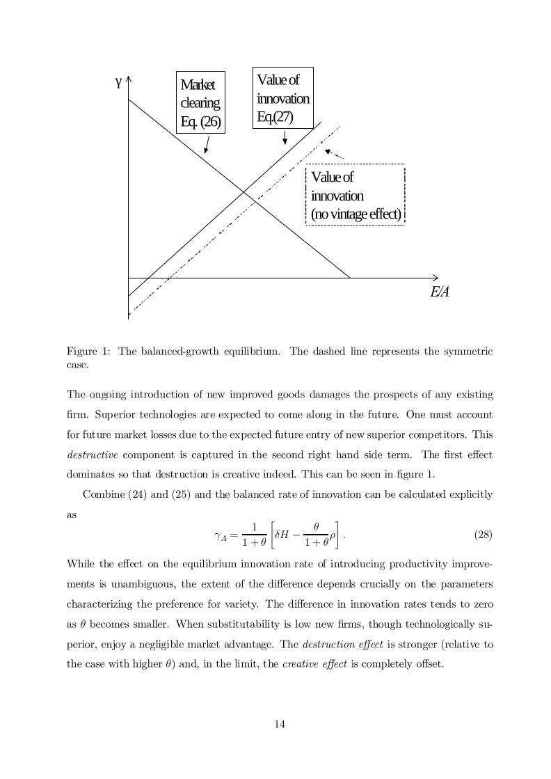
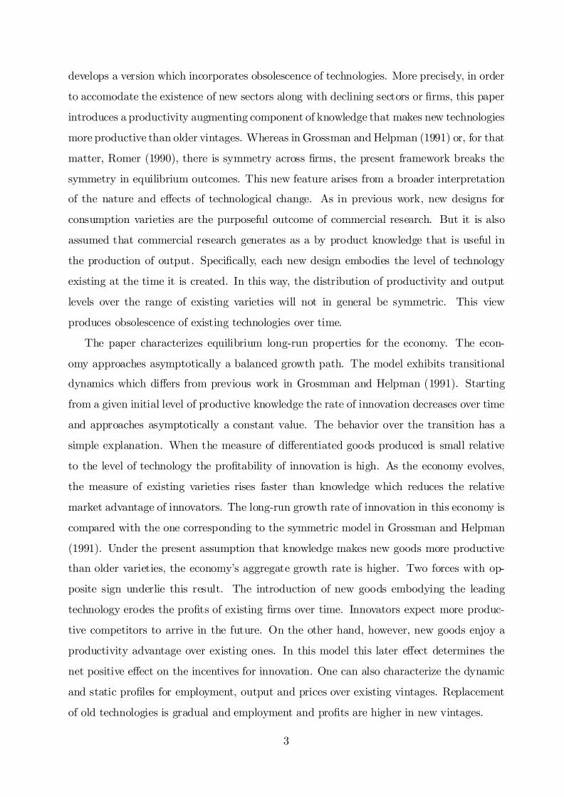
MarketclearingEq. (26)

Value ofinnovationEq.(27)

E/A

γ

Value ofinnovation(no vintage effect)

Figure 1: The balanced-growth equilibrium. The dashed line represents the symmetriccase.

The ongoing introduction of new improved goods damages the prospects of any existing

…rm. Superior technologies are expected to come along in the future. One must account

for future market losses due to the expected future entry of new superior competitors. This

destructive component is captured in the second right hand side term. The …rst e¤ect

dominates so that destruction is creative indeed. This can be seen in …gure 1.

Combine (24) and (25) and the balanced rate of innovation can be calculated explicitly

as

°A =1

1 + µ

"±H ¡ µ

1 + µ½

#: (28)

While the e¤ect on the equilibrium innovation rate of introducing productivity improve-

ments is unambiguous, the extent of the di¤erence depends crucially on the parameters

characterizing the preference for variety. The di¤erence in innovation rates tends to zero

as µ becomes smaller. When substitutability is low new …rms, though technologically su-

perior, enjoy a negligible market advantage. The destruction e¤ect is stronger (relative to

the case with higher µ) and, in the limit, the creative e¤ect is completely o¤set.

14

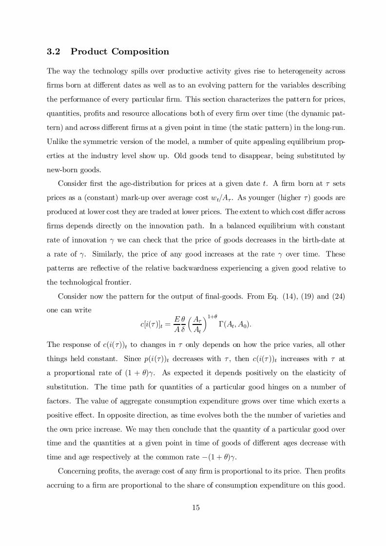
3.2 Product Composition

The way the technology spills over productive activity gives rise to heterogeneity across

…rms born at di¤erent dates as well as to an evolving pattern for the variables describing

the performance of every particular …rm. This section characterizes the pattern for prices,

quantities, pro…ts and resource allocations both of every …rm over time (the dynamic pat-

tern) and across di¤erent …rms at a given point in time (the static pattern) in the long-run.

Unlike the symmetric version of the model, a number of quite appealing equilibrium prop-

erties at the industry level show up. Old goods tend to disappear, being substituted by

new-born goods.

Consider …rst the age-distribution for prices at a given date t. A …rm born at ¿ sets

prices as a (constant) mark-up over average cost wt=A¿ . As younger (higher ¿) goods are

produced at lower cost they are traded at lower prices. The extent to which cost di¤er across

…rms depends directly on the innovation path. In a balanced equilibrium with constant

rate of innovation ° we can check that the price of goods decreases in the birth-date at

a rate of °. Similarly, the price of any good increases at the rate ° over time. These

patterns are re‡ective of the relative backwardness experiencing a given good relative to

the technological frontier.

Consider now the pattern for the output of …nal-goods. From Eq. (14), (19) and (24)

one can write

c[i(¿ )]t =E

A

µ

±

µA¿At

¶1+µ¡(At; A0):

The response of c(i(¿))t to changes in ¿ only depends on how the price varies, all other

things held constant. Since p(i(¿))t decreases with ¿ , then c(i(¿ ))t increases with ¿ at

a proportional rate of (1 + µ)°. As expected it depends positively on the elasticity of

substitution. The time path for quantities of a particular good hinges on a number of

factors. The value of aggregate consumption expenditure grows over time which exerts a

positive e¤ect. In opposite direction, as time evolves both the the number of varieties and

the own price increase. We may then conclude that the quantity of a particular good over

time and the quantities at a given point in time of goods of di¤erent ages decrease with

time and age respectively at the common rate ¡(1 + µ)°.Concerning pro…ts, the average cost of any …rm is proportional to its price. Then pro…ts

accruing to a …rm are proportional to the share of consumption expenditure on this good.

15

From (13), (19), and (23) the pro…t rate of a …rm can be written as

¼[i(¿ )]t =E

A

µA¿At

¶µ¡(At; A0):

So pro…ts fall with t and rise with ¿ at the rate ¡µ°A.

The economy is endowed with a …xed amount of primary factor. In a balanced equilib-

rium, the splitting of resources between research and …nal-goods is constant. It is interesting

to look now at the allocation of primary input among …rms. It results from the tension

between two forces. As already seen, younger …rms produce a larger quantity of good. On

the other hand they are more productive. We have that the …rst e¤ect dominates so that

more advanced …rms use a larger amount of primary factor. The quantity of employed

resources by individual …rms in Eq.(16) then decreases with the age of the …rms at a rate

¡µ°A.

Over time however for a particular …rm the demand of primary factor evolves according

to the demand for its product. Then employment in a …rm decreases over time at the same

rate as consumption does ¡(1 + µ)°A.

Going from individual …rms to age-groups of …rms, the distribution of input across

vintages ¿ is given by °c(¿ ). The lower the age of a set of …rms the higher the amount of

input employed there for two reasons: …rst each …rm individually uses a larger amount of

factor and, second, the number of …rms in that set is larger than in any other older set. It

is worth noting that the amount of primary factor employed by a new-born …rm decreases

over time. The whole set of forefront …rms at time t employs a constant amount °Ac(t) of

primary factor. Since the number of new …rms becomes larger, the amount employed by

any of them decreases at a rate ¡°.

3.3 Dynamics and existence

This subsection describes the dynamic adjustment of the economy that starts from an

initial level of knowledge A0. The analysis permits to identify existence conditions for the

type of long-run outcomes we have described above. Having de…ned z ´ E=A, it is useful

to rewrite the equations for equilibrium dynamics (21) and (25) as follows

° = ±h¡ µ

1 + µz

16

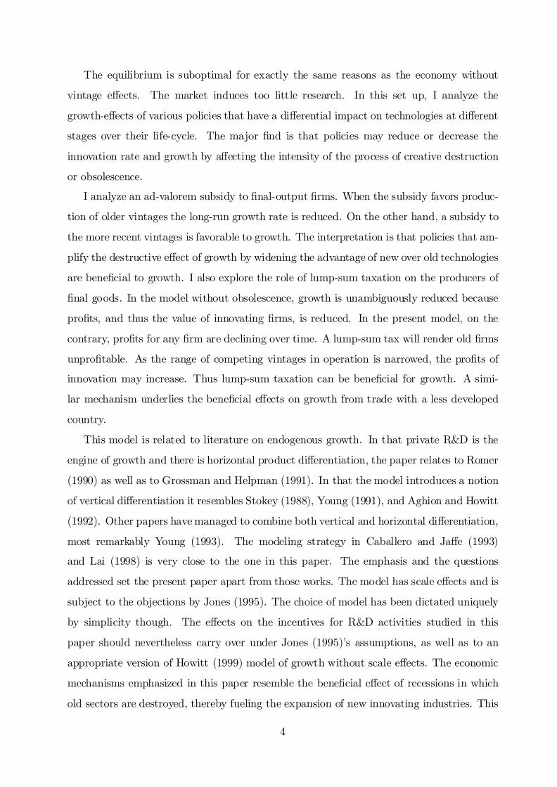
γ=0

∆z=0

At

z

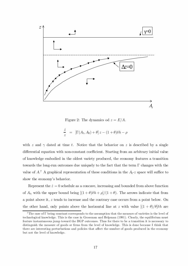
Figure 2: The dynamics od z = E=A.

_z

z= [¡(At; A0) + µ] z ¡ (1 + µ)±h¡ ½

with z and ° dated at time t. Notice that the behavior on z is described by a single

di¤erential equation with non-constant coe¢cient. Starting from an arbitrary initial value

of knowledge embodied in the oldest variety produced, the economy features a transition

towards the long-run outcomes due uniquely to the fact that the term ¡ changes with the

value of A.7 A graphical representation of these conditions in the At-z space will su¢ce to

show the economy’s behavior.

Represent the _z = 0 schedule as a concave, increasing and bounded from above function

of At; with the upper bound being [(1 + µ)±h+ ½]=(1 + µ). The arrows indicate that from

a point above it, z tends to increase and the contrary case occurs from a point below. On

the other hand, only points above the horizontal line at z with value [(1 + µ)=µ]±h are

7The case of ¡ being constant corresponds to the assumption that the measure of varieties is the level oftechnological knowledge. This is the case in Grossman and Helpman (1991). Clearly, the equilibrium mustfeature instantaneous jump toward the BGP outcomes. Thus for there to be a transition it is necessary todistinguish the measure of goods or …rms from the level of knowledge. This is done because I think thatthere are interesting perturbations and policies that a¤ect the number of goods produced in the economybut not the level of knowledge.

17

consistent with a path with positive innovation [i.e. increasing A over time]. It is simple to

see that, in the case this horizontal line falls below the upper bound for the _z = 0 schedule,

then for any choice of initial z we have that either A falls, or E attains negative values, or

innovation becomes zero in …nite time. Thus a necessary condition for positive innovation

to be sustainable is1 + µ

µ±h > ±h +

1

1 + µ½:

Under this condition the graphical analysis shows that we can …nd an initial value for z

such that the economy follows a path of perpetual growth. This path must be above _z = 0

approaching it as A grows. Thus consumption expenditure grows faster than knowledge

and the ratio between the two approaches the long-run value, which, consistently with out

interpretation, implies that the rate of pro…t on new goods decreases as the measure of

varieties produced increases. Accordingly the innovation rate declines monotonically to its

long-run value.

3.4 Welfare

The economy contains potential e¤ects for the edge between the market outcome and the

optimal social allocations. It is not hard to show however that the market equilibrium

di¤ers from the social optimum for the same reasons as in the economy without vintage

e¤ects. In particular, the static allocation of input across vintages is optimal. On the

other hand, the planner’s allocation of inputs to research exceeds the equilibrium one, thus

making research insu¢cient in equilibrium. But the wedge is determined by the standard

intertemporal spillover e¤ect. This can be seen by solving the planner’s optimal control

problem to …nd that the optimal growth rate exceeds the equilibrium growth rate by factor

1 + µ, just as in the symmetric version analyzed by Grossman and Helpman (1991). The

details of the argument are in appendix A. Market prices and interest rate re‡ect the

creative destruction behind obsolescence in a socially e¢cient way. Thus the same type of

R&D subsidy would be a …rst best policy.8 The next section will analyze other policies

that cannot typically be studied in models where goods are all symmetric.

8Lai (1998) discusses at length welfare e¤ects in a similar context. The present result suggests that thepresence of new welfare e¤ects is related to aspects of his model other than obsolescence.

18

4 Policies

The virtue of the model developed thus far is that clarity is preserved while incorporating

obsolescence and heterogeneity of …rms or sectors. This is interesting because this allows

the analysis of the growth e¤ects of policies that may have a di¤erential impact on dif-

ferent vintages. Selective subsidies are observed in practice. Subsidies are an instrument

that governments use to alleviate the loss of pro…ts and employment in certain …rms and

sectors. In other cases, this type of interventions are deployed to prop up new emergent

sectors. In the model, these policies bring about growth e¤ects by interfering the process

of creative destruction. Other policies such as lump-sum taxes and trade policies will also

have consequences for the allocation of resources to growth generating activities through a

similar channel.

4.1 Production Subsidies

Assume a a …rm i is subsidized at the rate ´(i)t, which may change over time. Given that

the demand of this good x(i)t is exactly as before pro…ts are

¼(i)t = x(i)t

"p(i)t(1 + ´(i)t)¡

wtÁ(At(i))

#

Pro…t maximization implies mark-up pricing on a variable cost wt=Á((At(i))(1 + ´(i)t))

which now includes the fact that a positive ad-valorem subsidy allows the …rm to sell at a

lower price. Assuming, as before, that Á(A) = A is given as in Eq. (22), the analogous to

Eq. (13) and (14) are, respectively,

c(i)t =EtAt

µ

1 + µ

1

±

(1 + ´(i)t)1+µA1+µt(i)R nt(1 + ´(j)t)µAµt(j)dj

and

¼(i)t = Et1

1 + µ

(1 + ´(i)t)1+µAµt(i)R nt(1 + ´(j)t)µAµt(j)dj

It is apparent that the market position and thus the value of a …rm will depend on the

overall distribution of subsidy rates over vintages. Certainly, most often subsidies are not

set for all the goods produced in the economy, but they are designed to protect speci…c

sectors or groups of producers. The details of the analysis are in appendix B.

19

4.1.1 Protection of declining sectors

For example, governments have used subsidies to help declining sectors. The target consists

of sectors that have experienced a long-process of job destruction and reduction in pro…t

rates. In terms of our model, the bene…ciaries of such a policy would be the oldest vintages.

Provided that this policy will certainly keep old …rms from declining too fast, we want to

asses the implications for the overall performance of the economy. To this end, assume that

´(i)t = ´ for i such that t(i) < t ¡ T , and ´(i)t = 0 otherwise. That is, all …rms aged T

and over bene…t from the constant subsidy. It is convenient to de…ne

¡s1(At) ´ A1+µt

(1 + ´)µhA1+µt¡T ¡ A1+µ0

i+

hA1+µt ¡ A1+µt¡T

i (29)

which, as ¡(:) in Eq.(23), re‡ects the competitiveness of the leading technology relative to

the whole set of existing …rms. In this case, the presence of ´ shows that older …rms are

now relatively more competitive thus reducing the edge of the state-of-the-art …rms. I will

focus on long-run balanced outcomes with constant innovation rate ° so the role of A0 can

safely be ignored. The expressions for quantities and pro…ts in Eq.(13) and (14) can now

be written as

c(i)t =EtAtµ1

±

ÃAt(i)At

!1+µ(1 + ´(i))1+µ¡s1(At) (30)

¼(i)t =EtAt

ÃAt(i)At

!µ(1 + ´(i))1+µ¡s1(At) (31)

This equations can be used to develop the two main equilibrium equations. As for the

derivation of Eq. (21), the block of conditions (1), (15), (16) and (19) now leads up to a

condition that re‡ects the market clearing allocation of the primary input to research

° = ±h ¡ µ

1 + µ

E

A

1 + e¡°(1+µ)T ((1 + ´)1+µ ¡ 1)1 + e¡°(1+µ)T(´1+µ ¡ 1) (32)

The second term on the right-hand side describes the allocation of inputs to the production

of consumption goods rather than research. The expression shows that the presence of the

20

subsidy increases the demand of inputs for …nal-good production and is detrimental to

research. This negative e¤ect is smaller the older the recipient …rms since those …rms

take up relatively fewer resources. Graphically, the negatively-sloped line in …gure 1 shifts

downwards.

The second condition is related to the equilibrium returns to innovation activities.

Again, just as for the derivation of Eq. (25), the set of conditions (18) and (8) permit

to derive the following

° =E

A

1 + e¡½T e¡°(1+µ)T ((1 + ´)1+µ ¡ 1)1 + e¡°(1+µ)T ((1 + ´)µ ¡ 1) ¡ µ° ¡ ½ (33)

The term accompanying E=A picks up the role of the subsidy for the returns to innovation.

The net sign of this e¤ect is ambiguous. On one hand, the subsidy increases the present

value of the …rm and thus the return to creating a new product. However, the subsidy also

increases the competitiveness of the rest of …rms which tends to erode the ‡ow of pro…ts.

The direct bene…ts occur in the future and are discounted, thus when discount is high or

the period to qualify for the subsidy, T , is long then the subsidy scheme is more likely to be

detrimental for the return to investment. In terms of …gure 1, the positively sloped curve

may shift either way.

In general equilibrium, nonetheless, the net e¤ect of subsidies is unambiguously negative

on growth. Combining the two above conditions Eq.(32) and (33) shows that the long-run

rate of innovation is smaller than when ´ = 0, and that it declines with the value of ´ and

with the value of T . Analytically, the equilibrium ° is determined by

1 + e¡½Te¡°(1+µ)T((1 + ´)1+µ ¡ 1)1 + e¡°(1+µ)T ((1 + ´)1+µ ¡ 1) =

(1 + µ)° + ½

±h¡ °µ

1 + µ:

The forces at work are as follows. On one hand, the value of …rms becomes higher

because the subsidy increases pro…ts from age T on. On the other hand, since subsidized

…rms increase their demand for inputs, there is less productive factor left for research. It

turns out that the e¤ect on the value of the …rms is small relative to the impact on the

demand for input by …rms. The reason is that the former is discounted since it occurs far

in the future. What is important to stress is that it is not the presence of subsidies per se

that reduces the allocation of resources to growth-generating activities, but its distribution

21

across …rms of di¤erent vintages. If all goods were subsidized [i.e. T = 0] then the subsidy

rate ´ would not have any bearing on equilibrium innovation.

4.1.2 Infant industry protection

The opposite case that subsidies are targeted at the newest …rms is considered next. I …nd

that such a scheme creates a wider advantage of innovators over the average existing …rm.

This produces a larger incentive for undertaking research. To make this case, assume that

at t there is a positive subsidy rate only for …rms born after t¡ T . Assume that ´(i)t = ´

for i such that t(i) > t ¡ T , and ´(i)t = 0 otherwise.

For this case, it is useful to de…ne

¡s2(At) ´ A1+µt

A1+µt¡T ¡ A1+µ0 + (1 + ´)µhA1+µt ¡ A1+µt¡T

i (34)

Again, this is re‡ective of the relative market position. The qualitative e¤ect of the subsidy

is as in ¡s1 as de…ned in Eq.(28) above, but here this subsidy improves the relative compet-

itiveness of younger rather than older vintages. The equilibrium expressions for quantities

and pro…ts in Eq. (30) and (31) also apply provided that ¡s1 is replaced by ¡s2. Proceeding

as in the previous cases, the market-clearing related condition leads to the expression

° = ±h¡ µ

1 + µ

E

A

(1 + ´)1+µ(1¡ e¡°(1+µ)T ) + e¡°(1+µ)t(1 + ´)µ(1¡ e¡°(1+µ)T ) + e¡°(1+µ)t (35)

which describes the incentives governing the allocation of inputs to research and …nal-

goods production. As before, for given E=A, the subsidy leads to less resources to research.

Graphically, the positive curve in …gure 1 shifts downwards. On the other hand, the study

of the return to innovations produces the other equilibrium equation

° =E

A

(1 + ´)1+µ(1 ¡ e¡½T e¡°(1+µ)T ) + e¡½T e¡°(1+µ)T(1 + ´)µ(1¡ e¡°(1+µ)T ) + e¡°(1+µ)T ¡ µ° ¡ ½ (36)

The e¤ect of ´ here is unambiguously positive. The innovator enjoys the subsidy edge right

from the start of its activity, and the drop in pro…t due to the future withdrawal of the

subsidy is discounted. Graphically, the negatively-sloped curve shifts upwards in …gure 1.

In general equilibrum, the direct impact on the pro…tability of research dominates so

22

that the subsidy increases the rate of innovation. This can be seen explicitly by combining

Eq.(35) and (36) to obtain

(1 + ´)1+µ ¡ e¡½T e¡°(1+µ)T ((1 + ´)1+µ ¡ 1)(1 + ´)1+µ ¡ e¡°(1+µ)T((1 + ´)1+µ ¡ 1) =

(1 + µ)° + ½

±h ¡ °µ

1 + µ:

Again, a subsidy that applies to everyone (T ! 1) has no growth e¤ect, showing the

importance of the selective character of this policy. Whereas the growth e¤ect is welfare

improving, this subsidy also produces a static distortion. To judge whether this policy is

bene…cial the dynamic bene…ts must be balance against the losses created by the distortion.

4.2 Lump-sum Taxes

Business taxation usually has an important lump-sum component. Here I assume there is

a …xed tax f collected of …rms producing consumption goods. Since a …rm’s gross pro…t

declines over time, this …xed tax per period will imply that current net pro…ts for some …rms

will become negative. At this point, any such a …rm will shut down and stop operating.

The …rms that will drop out of the produced set will be those aged T an above for some

T that has to be determined. More formally, Eq.(12) still characterizes the pricing rule of

a …rm i. Provided that the range of varieties is not …nite, following an analysis similar to

that in section 4.1 delivers the following equations for gross pro…t rates and quantities

c(i)t =EtAt

µ

±

ÃAt(i)At

!1+µ¡f(At; At¡T ) (37)

¼(i)t =EtAt

ÃAt(i)At

!µ¡f (At; At¡T) (38)

with

¡f(At; At¡T) ´ A1+µt

A1+µt ¡ A1+µt¡T=

1

1¡ e¡°(1+µ)T ; (39)

where the second equality uses the constant-growth assumption.

23

Now one can calculate the age T at which a …rm will be discontinued. To that end, set

¼(i(t))t+T =Et+TAt+T

ÃAtAt+T

!µ¡f (At+T ; At)¡ f = 0;

which, on a BGP with At+T = exp(°T)At and constant E=A delivers the relation between

f and T given ° and E=A

E

Ae¡°µT

1

1¡ e¡°(1+µ)T = f: (40)

One can show that the equation related to market clearing can be found by rearranging

(1), (15), (16) and (19) to yield the same equation (26) as in the model without policies,

which is reproduced again as

° = ±h¡ µ

1 + µ

E

A: (41)

The condition related to the return from innovations will be a¤ected though. Using

Eq.(8) and the normalization V [i(t)]t = 1 one can show that

r =EtAt¡(At; At¡T )¡ µ° ¡ µ° 1

rf

³1¡ e¡rT

´:

Comparing this with Eq.(20) with (22) reveals a number of e¤ects of the tax f on the

equilibrium return to innovations. The term ¡f(:) indicates that a new …rm will be more

pro…table since the range of competitors is narrowed as consequence of the tax. The last

term accounts for the negative e¤ects of the tax on the pro…ts …rms can produce. With

Eq.(18) and (38), the above expression leads to the other equilibrium equation

° =EtAt

1

1¡ e¡°(1+µ)T ¡ µ° ¡ µ° 1rf

³1 ¡ e¡(°+½)T

´¡ ½ (42)

Given the tax f, the balanced-growth equilibrium consists of values for T , ° and E=A

that satisfy Eq. (40), (41) and (42). As shown in appendix C, with a positive lump-sum

tax, the innovation rate will be higher than without the tax if and only if

µ°

° + ½(e°T ¡ e¡½T) < 1:

24

For T small enough, ° is higher than without f . Using the shut-down condition Eq.(40),

for every such a T , and the corresponding ° and E=A, a value of the tax f can be found

that generates this equilibrium. It can then be concluded that for large enough f growth

increases with a lump-sum tax.

This result stands in stark contrast with the one implied by the model without obsoles-

cence and symmetric goods of Grossman and Helpman (1991). In that case, a lump-sum

tax is unambiguously detrimental for growth through its negative e¤ect on pro…t rates.

4.3 Trade and Openness

In this section, it is considered the case that the economy engages in trade with a foreign

country that has a lower level of technological development. Formally, denote by ~At the level

of knowledge reached by this foreign partner at time t. The assumption is that At= ~At > 1.

Since the focus is on balanced-growth situations, I will assume that this gap is constant

over time so both countries are growing at the same rate. Therefore, it takes a constant

period T for the foreign country to catch up with the domestic country’s technology, so that

~At+T = At all t. This implies that At= ~At = exp(°T). I will further assume that the wage in

the foreign economy, ~w, is lower than that in the domestic economy w and that the gap is

such that all goods that are technologically feasible in the foreign country [i.e. i � ~A] will

be produced there. In other words, over time old varieties formerly produced domestically

will eventually be produced in the foreign country.9 This scenario thus captures the features

of the international product cycle studied by Vernon (1966) and Stokey (1991). Firms in

both countries operate under conditions of monopolistic competition, so the pricing rule

for goods will now be

p(i)t =1+ µ

µ

1

At(i)£

8><>:

wt i > ~At

~wt i � ~At

De…ne the term that represents the relative competitiveness of an innovator in the open

domestic country as follows.

¡o(At; ~At) ´ A1+µt³wt~wt

´µ( ~A1+µt ¡ A1+µ0 ) + (Aµt ¡ ~A1+µt )

=e°(1+µ)T

³wt~wt

´µ+ e°(1+µ)T ¡ 1

< 1;

9Mateos-Planas (1998) shows that this set of assumptions is consistent with the implications of a two-country general equilibrium model with imitation, rather than R&D, in the foreign country.

25

where the equality follows from the assumptions made about the technological gap, and the

inequality is from the assumption ~w < w. Observe that for the closed economy analyzed in

section 3, the balanced-growth value of ¡ in Eq. (23) is unity. This indicates that a domestic

innovator in the open economy faces …ercer competition from low-wage producers located

in the foreign country. On its own, that would tend to have a detrimental e¤ect on the

incentives to conduct research. The net e¤ect depends on a larger number of interactions.

To work out these e¤ects, start again with the relation related to clearing in the domestic

market for the primary input. This leads to

° = ±h ¡ µ

1 + µ

E

A¡o(At; ~At)

241 ¡

à ~AtAt

!1+µ35

= ±h ¡ µ

1 + µ

E

A¡o(At; ~At)(1¡ e¡°(1+µ)T)

Comparison with Eq.(26) corresponding to the closed economy indicates that in the open

economy foreign competition in the production of …nal goods frees resources for research.

In terms of …gure 1, the curve with negative slope shifts upwards with trade.

The second equilibrium condition that relates to the market value of innovation for the

open economy reads

° =E

A¡o(At; ~At)(1 ¡ e¡(r+°µ)T )¡ µ° ¡ ½:

This di¤ers from Eq.(27) that corresponds to the closed economy. As mentioned earlier,

trade with a low-wage country reduces current pro…ts as well as the lifetime span of an

innovating …rm in the high-wage domestic economy. Graphically, the curve with positive

slope in …gure 1 will shift downwards with openness. Combining the two last equations,

the net e¤ect of trade can be determined. It is convenient to de…ne

'(T; °) ´ 1 ¡ e¡°(1+µ)T1¡ e¡(½+(1+µ)°)T :

Then the equilibrium growth rate must satisfy

° =1

1 + µ'(T; °)

"±h¡ µ

1 + µ½'(T; °)

#;

26

which is to be compared with the closed-economy expression in Eq.(28). Since '(T; °) < 1,

growth for the open economy is higher. This outcome is driven by the diversion of resources

from …nal-goods production into research that occurs when foreign competition intensi…es

the process of economic obsolescence of existing domestic technologies.

5 Conclusions

This paper studies a model of growth where technological change has an embodied compo-

nent that makes new vintages of …rms more productive. The phenomenon of obsolescence

is a feature of the growth process whereby new sectors or …rms replace existing ones. The

transitional and long-run properties of the economy are investigated. The analysis identi…es

policies that have e¤ects on growth through their in‡uence on the course of the creative

destruction associated with the ongoing process of emergence and obsolescence of …rms and

sectors.

This paper shows that subsidies targeted at young innovative sectors or …rms will have a

positive growth e¤ect. On the contrary, subsidies aimed at older vintages will be detrimental

for growth. These growth e¤ects arise entirely from the selective nature of the policies. A

uniform non-selective subsidy would have no growth e¤ect. Similarly, a lump-sum tax on

…rms in the economy that forces the old less-pro…table …rms to shut down may have a

positive e¤ect on growth. It is interesting that, in the absence of obsolescence, a lump-sum

tax of the type analyzed here would reduce the growth rate unambiguously. The degree

of openness to international trade of a more developed economy with a less developed

partner will also be growth-enhancing for similar reasons. Foreign competition moves the

production with old technologies to the foreign country and releases resources for innovation

at home.

The main contribution of this paper is to demonstrate that, once obsolescence is ac-

counted for, new and potentially important growth-e¤ects of policies show up. The study

of these e¤ects necessarily demands a model that, like the one proposed in this paper,

accommodates heterogeneous …rms and sectors.

This paper stops short of producing a detailed welfare analysis of the policies considered.

In particular, selective subsidies to innovative sectors have a dynamic welfare bene…t but

produce a static loss. The net welfare e¤ects of this and other policies deserve to be

27

investigated in future work.

The model used in this paper is very stylized and is thus bound to have limitations.

The analytical simplicity of the model comes at the cost of sacri…cing the possibility of

relating the model to observable data on sectors and industries. But a more quantitatively

oriented approach would be required to assess the practical signi…cance of the e¤ects of the

policies considered in this paper. Such an approach would also be necessary to evaluate

the net welfare e¤ects of these policies.

28

References[1] Aghion, P. and P. Howitt. A Model of Growth Through Creative Destruction. Econo-

metrica, 60, 1992.

[2] Caballero R. J. and M. Hammour. The Cleansing E¤ect of Recessions. AmericanEconomic Review, 84, 5, December, 1994.

[3] Caballero R. J. and A. B. Ja¤e. How High Are the Giants’ Shoulders: an EmpiricalAssesment of Knowledge Spillovers and Creative Destruction in a Model of EconomicGrowth. NBER Macroeconomics Annual, 1993.

[4] Dixit, A. and J. Stglitz. Monopolistic Competition and Optimal Product Diversity.American Economic Review, 67, 1977.

[5] Grossman G. and E. Helpman. Protection for Sale. American Economic Review, 84,1994.

[6] Grossman G. M. and E. Helpman. Innovation and Growth in the Global Economy.M.I.T. Press, 1991.

[7] Hillman, A. L. . Declining Industries and Political SupportProtectionist Motives.American Economic Review, 72, 1982.

[8] Jones, C. I. R&D Models of Endogenous Growth. Journal of Political Economy, 103,1995.

[9] Howitt, P. Steady Endogenous Growth with Population and R&D Inputs Growing.Journal of Political Economy, 107, 1999.

[10] Krueger, A. O. Government Failures in Development. Journal of Economic Perspec-tives, 4, 3, 1990.

[11] Lai, E. Schumpeterian Growth with Gradual Product Obsolescence. Journal of Eco-nomic Growth, 3, 1998.

[12] Maggi, G. and E. Rodriguez-Clare. Import Penetration and the Politics of TradeProtection. NBER Working Paper 6711, 1998.

[13] Mateos-Planas, X. Trade, the Product Cycle, and the International Production Pat-tern. Mimeo, 1998.

[14] Mokyr, J. The Lever of Riches: Technological Creativity and Economic Progress,Oxford University Press, 1990.

[15] Pack, H. and L. E. Westphal. Industrial Strategy and Technological Change: Theoryversus Reality. Journal of Development Economics, 22, 1986.

[16] Parente, S. Technology Adoption, Learning-by-Doing and Economic Growth. Journalof Economic Theory, 63, 1994.

[17] Romer, P. Endogenous Technological Change. Journal of Political Economy, 98, 1990.

29

[18] Rosenberg, N. Inside the Black Box: Technology and Economics. Cambridge Univer-sity Press, 1982.

[19] Schumpeter, J. A. Capitalism, Socialism and Democracy, New York: Harper, 1942.

[20] N. Stokey. Learning by Doing and the Introduction of New Goods. Journal of PoliticalEconomy, 96, 1988.

[21] N.Stokey. The Volume and Composition of Trade Between Rich and Poor Countries.Rev Ec Studies, 1991.

[22] Tre‡er, D. "Trade Liberalization and te Theory of Endogenous Protection. Journalof Political Economy, 101, 1994.

[23] Vernon. International Investment and International Trade in the Product Cycle. Quar-terly Journal of Economics, 80, 1966.

[24] Westphal L. E.. Industrial Policy in an Export-Propelled Economy: Lessons fromSouth Korea’s Experience. Journal of Economic Perspectives, 4, 3, 1990.

[25] Young, A. Invention and Bounded Learning by Doing. Journal of Political Economy,101, 1993.

[26] Young, A. A Tale of Two Cities: Factor Accumulation and Technical Change inHong-Kong and Singapore. NBER Macroeoconomics Annual, 1992.

[27] Young, A. Learning by Doing and the Dynamic E¤ects of International Trade. Quar-terly Journal of Economics, 106, 1991.

30

A Welfare AnalysisThe planner’s static problem consists of maximizing

Z n

0c(j)®dj

subject to the constraint

hc =

Z n

0

c(j)

At(j)dj;

where hc denotes the amount of primary input available in the consumption good sector. Thesolution to this problem delivers the optimal allocation of this input across existing sectors at atime t:

c(i)t = hcA1+µt(i)

11+µ(A

1+µt ¡ A1+µ0 )

:

In the market equilibrium the same condition holds provided that there hc = (µ=(1 + µ))(h +(1=(1 + µ))(½=±)). This allows the computation of the indirect utility as

Z nt

0c(i)tdi = hµ=(1+µ)c At

µ1

1 + µ

¶1=(1+µ)= h®cAt(1 ¡ ®)®=(1¡®)

where the 2nd equality uses the de…nition of µ in Eq. (6). For the sake of comparison, in thesymmetric case the exponent on A is smaller (1 ¡ ®)=®.

The planner’s dynamic problem is the choice of the paths for A and hc that maximize therepresentative households utility. The Hamiltonian associated with this problem is

H = e½t log((1 ¡ hr)A1=®) + ¹(±hrA):

The solution on a BGP leads to the optimal

h¤r = h ¡ ®

±½ = h¡ µ

1 + µ

½

±:

The resulting optimal growth rate is

°¤ = ±(h¡ ®½

±):

Comparing with the market growth rate ° in Eq. (31) shows that °¤=° = 1=(1 ¡ ®). Thesame holds for the symmetric economy analyzed by Grossman and Helpman (1991).

B SubsidiesConsider production is subsidized at rates ´(i)t. As with the basic model, the equilibrium hastwo main relations. The …rst comes from market clearing that determines the amount of labor toR&D. This is still given by equations (1), (15), (16), and (19). The other relation follows fromthe equilibrium valuation of innovations. Again, this consists of equations (18) and (8) [or (20)].These relations are incomplete though. To close the model, one needs to determine the e¤ect ofthe subsidy on the amount of the di¤erentiated consumption goods and the pro…t rate.

Equation (6) still holds for the demand of each intermediate. If i is subsidized at the rate ´(i)then pro…ts are

¼(i)t = x(i)t

"p(i)t(1 + ´(i)t) ¡ wt

Á(At(i))

#

31

The FOC for pro…ts maximization becomes,

x(i)t[¡(1 + µ)(1 + ´(i)t) +wt

p(i)tÁ(At(i))(1 + µ) + (1 + ´(i)t)] = 0

implies mark-up pricing,

p(i)t =1 + µ

µ

1

1 + ´(i)t

wtÁ(At(i))

Assuming, as before, that Á(A) = A, the quantity produced and sold by the …rm is,

x(i)t = Etµ

1 + µ

1

wt

(1 + ´(i)t)1+µA1+µt(i)R nt(1 + ´(j)t)µAµt(j)dj

With this equations, the pro…t rate becomes

¼(i)t = Et1

1 + µ

(1 + ´(i)t)1+µAµt(i)R nt(1 + ´(j)t)µAµt(j)dj

Now the expressions for quantities and pro…ts can be used in the derivation of the two mainequilibrium equations. This will be done for the di¤erent types of policies separately.

Protection of declining sectorsAssume that ´(i)t = ´ for j such that t(i) < t ¡T , and ´(i)t = 0 otherwise. That is, all …rms

over age T bene…t from the constant subsidy. With ¡(At; A0) as de…ned in the main text Eq.(23)

¡(At) ´ A1+µt

(1 + ´)µhA1+µt¡T ¡ A1+µ0

i+

hA1+µt ¡ A1+µt¡T

i

We will focus on long-run balanced outcomes with constant innovation rate °. In this context

¡(At ! ¡1 =1

(1 + ´)µ¡e¡°(1+µ)T ¡ e¡°(1+µ)t

¢+1 ¡ e¡°(1+µ)T

From the abov expression for c(i),

c(i)t = Etµ

1 + µ

1

wt

(1 + ´(i))1+µA1+µt(i)

11+µ

n(1 + ´)µ

hA1+µt¡T ¡A1+µ0

i+

hA1+µt ¡ A1+µt¡T

io

= Etµ1

wt

(1 + ´i)1+µA1+µt(i)

(1 + ´)µhA1+µt¡T ¡A1+µ0

i+

hA1+µt ¡ A1+µt¡T

i

= Etµ1

wt

µAt(i)At

¶1+µ(1 + ´)1+µ¡(At)

We can recover the expression for pro…ts as,

¼(i)t =1

µ

wtAt(i)

x(i)t

= Et(1 + ´(i))1+µAµt(i)

(1 + ´)µhA1+µt¡T ¡A1+µ0

i+

hA1+µt ¡ A1+µt¡T

i

=EtAt

µAt(i)At

¶µ(1 + ´)1+µ¡(At)

32

Market clearingThe block of equilibrium equations (1), (15), (16), and (19) can now be developed. The

factor-market clearing condition (15)

hrt +

Z nth(i)tdi = H

with the law-of-motion of knowledge (1) with (2) , _AtAt1± = hrt, R&D equilibrium condition (19)

wt = ±At and factor demand functions (16) h(i)t = x(i)tAt(i)

, yield a condition for any equilibriumwith positive innovation. First,

Z nth(i)tdi = Etµ

1

wt¡(At)

µ1

At

¶1+µ

£(Z t¡T

Aµ¿ (1 + ´)1+µ _A¿d¿ + +

Z t

t¡TAµ¿ _A¿d¿

)

= Etµ1

wt¡(At)

µ1

At

¶1+µ 1

1 + µ

£n(1 + ´)1+µ

hA1+µt¡T ¡ A1+µ0

i+

hA1+µt ¡ A1+µt¡T

io

Using that w = ±A in Eq.(19), and considering long-run outcomes market clearing can beposed,

h = °1

±+

µ

1 + µ

1

±

EtAt

¡(At;A0)h(1 + ´)1+µ

³e¡°(1+µ)T ¡ e¡°(1+µ)t

´+ 1 ¡ e¡°(1+µ)T

i

For graphical representation we will use the BGP relation,

E

A=

±h¡ °

¡1£(1 + ´)1+µe¡°(1+µ)T + 1 ¡ e¡°(1+µ)T

¤ 1 + µ

µ

Market valuationThe other equilibrium equation analogous to Eq. (23) comes from the analysis of …rms’

valuation and the no-arbitrage condition. Letting V (¿)t denote the present (fundamental) valueof a …rm in cohort ¿ at time t. I …nd that

dV (t)tdt

= _V (t)t + °V (t)t + e¡R t+T

trudu¼(t)¡t+T ¡ e¡

R t+T

trudu¼(t)+t+T ;

with¼(t)+t+T = (1 + ´)1+µ¼(t)¡t+T;

and

¼(t)¡t+T =Et+TAt+T

µAt

At+T

¶µ¡(At+T):

We use the normalization:V (t)t = 1:

33

In a BGP with constant r and °

dV (t)tdt

= _V (t)t + µ° + e¡rT (¼(t)¡t+T ¡ ¼(t)+t+T ) =

= _V (t)t + µ° + e¡rTEt+TAt+T

µAt

At+T

¶µ¡(At+T )(1 ¡ (1 + ´)1+µ) = 0

With the no-arbitrage condition

r = ¼(t)t + _V (t)t

and the fact that

¼(t)t =EtAt

¡(At)

we get

r =EtAt

¡(At)¡ µ° + e¡rTEt+TAt+T

µAt

At+T

¶µ¡(At+T )((1 + ´)1+µ ¡ 1)

Finally, intertemporal optimality gives the behavior of consumption expenditures

_E

E= r ¡ ½;

so that in a BGP we have,

° =EtAt

¡(At)¡ µ° + e¡rTEt+TAt+T

µAt

At+T

¶µ¡(At+T )((1 + ´)1+µ ¡ 1) ¡ ½:

Or, rearranging,

(1 + µ)° =E

A¡1

h1 + e¡(r+°µ)T ((1 + ´)1+µ ¡ 1)

i¡ ½;

In the long-run consumption must grow at the same rate as knowledge and then r = ° + ½.Therefore, after rearranging, we get

E

A=

(1 + µ)° + ½

¡1[1 + e¡½T e¡°(1+µ)T ((1 + ´)1+µ ¡ 1)]

Balanced growth equilibriumCombining the two above conditions

1 + e¡½T e¡°(1+µ)T((1 + ´)1+µ ¡ 1)

1 + e¡°(1+µ)T ((1 + ´)1+µ ¡ 1)=

(1 + µ)° + ½

±h ¡°

µ

1 + µ:

Infant industry protectionTo make this case, we assume that there a positive subsidy rate only for …rms born after t¡T.

For this case, it is useful to rede…ne

¡(At) ´ A1+µt

A1+µt¡T ¡ A1+µ0 +(1 + ´)µhA1+µt ¡ A1+µt¡T

i

which along long-run balanced growth paths reads

34

¡1 =1

e¡°(1+µ)T + (1 + ´)µ(1 ¡ e¡°(1+µ)T )

Market clearingWith the de…niton of ¡(At;A0) in the text, market-clearing now requires,

h = °1

±+

µ

1 + µ

1

±

EtAt

¡(At)he¡°(1+µ)T + (1 + ´)1+µ(1 ¡ e¡°(1+µ)T )

i

which more conveniently can be written as,

E

A=

±h¡ °

¡1£(1 + ´)1+µ ¡ e¡°(1+µ)T ((1 + ´)1+µ ¡ 1)

¤ 1 + µ

µ

Market valuationOn the valuation side, normalizing value of innovations to one, we …nd that,

dV

dt= V 0

t + µ° + e¡rTE

A

µAt

At+T

¶µ¡1((1 + ´)1+µ ¡ 1) = 0:

Provided that ¼(t)t = (E=A)¡1(1 + ´)1+µ, the no-arbitrage condition r = ¼(t)t +V 0t implies

that

r = (E=A)¡1h(1 + ´)1+µ ¡ e¡rT e¡°µT((1 + ´)1+µ ¡ 1)

i¡ µ°:

Using that in BGP r = ° + ½ we arrive at

E

A=

(1 + µ)° + ½

¡1£(1 + ´)1+µ ¡ e¡½T e¡°(1+µ)T ((1 + ´)1+µ ¡ 1)

¤

Balanced growth equilibriumFrom the two long-run equilibrium equations we can study the determination of ° to determine

that larger ´ increases the rate of innovation. More explicitly,

(1 + ´)1+µ ¡ e¡½T e¡°(1+µ)T ((1 + ´)1+µ ¡ 1)

(1 + ´)1+µ ¡ e¡°(1+µ)T ((1 + ´)1+µ ¡ 1)=

(1 + µ)° + ½

±h¡ °

µ

1 + µ:

C Lump-sum taxationLet T denote the age of the oldest frim in operation. Following analysis similar to that in section3 delivers the following equations for gross pro…t rates and quantities

x(i)t =EtAt

µ

±

µAt(i)At

¶1+µ¡(At;At¡T )

¼(i)t =EtAt

µAt(i)At

¶µ¡(At;At¡T )

35

with

¡(At; At¡T ) ´ A1+µt

A1+µt ¡A1+µt¡T=

1

1 ¡ e¡°(1+µ)T

where the second equality uses the constant-growth assumption.Now one can calculate the age T at which a …rm will be discontinued. To that end, set

¼(i(t))t+T =Et+TAt+T

µAt

At+T

¶µ¡(At+T ;At) ¡ f = 0;

which, on a BGP with At+T = exp(°T)At and constant E=A delivers the relation between f andT given ° and E=A

E

Ae¡°µT

1

1 ¡ e¡°(1+µ)T= f:

One can show that the equation related to market clearing can be found by rearranging (1),(15), (16) and (19) to yield the same equation as in the model without policies,

° = ±h ¡ µ

1 + µ

E

A:

The condition related to the return from innovations will be a¤ected. Di¤erentiate the fun-damental value of the …rm to obtain

dV [i(t)]tdt

= _V [i(t)]t + µ°

Z t+T

te¡r(s¡t)[¼[i(t)]s + f ]ds

= _V [i(t)]t + µ°V [i(t)]t + µ°f(¡1=r)he¡r(s¡t)

it+Tt

= _V [i(t)]t + µ°V [i(t)]t + µ°f1

r

³1 ¡ e¡rT

´

Using Eq. (8) and the normalization V [i(t)]t = 1 constant it follows

r =EtAt

¡(At;At¡T ) ¡ µ° ¡ µ°1

rf

³1 ¡ e¡rT

´:

With Eq. (18) then

° =EtAt

¡(At;At¡T ) ¡ µ° ¡ µ°1

rf

³1 ¡ e¡(°+½)T

´¡ ½

=EtAt

1

1 ¡ e¡°(1+µ)T¡ µ° ¡ µ°

1

rf

³1 ¡ e¡(°+½)T

´¡ ½

Combine the market-clearing and the valuation conditions to substiture E=A out to obtain

(1 + µ)° + ½

(±h ¡°) 1+µµ=

1

1 ¡ e¡°(1+µ)T¡ µ° 1r f(1 ¡ e¡(°+½)T )

(±h¡ °)1+µµ

On the other hand, the shut-down condition with the market-clearing condition can be written as

f

(±h ¡°)1+µµ=

e¡°µT

1 ¡ e¡°(1+µ)T:

Combining the two last expressions gives an expression in ° and T

(1 + µ)° + ½

(±h ¡°)1+µµ=

1

1 ¡ e¡°(1+µ)T

�1 ¡ µ

°

° + ½e¡°µT (1 ¡ e¡(°+½)T )

¸

36

In the case without the tax f, the equilibrium ° is characterized by this equation when theleft-hand side is equal to 1. Therefore, under the lump-sum tax, the innovation rate will be higherif and only if

µ°

° + ½e¡°µT (1 ¡ e¡(°+½)T ) < e¡°(1+µ)T

or, after rearranging,µ

°

° + ½(e°T ¡ e¡½T ) < 1:

The left side is an incresing function of T , and for T small enough the inequality holds. It followsthat for T smaller than some value, ° is higher than without f . Using the shut-down condition, forevery such a T , and corresponding ° and E=A, an f can be found that generates this equilibrium.So the result is that there exist large enough values for f such that growth increases with alump-sum tax.

37