Discussion Papers in Economics

Department of Economics and Related Studies

University of York

Heslington

York, YO10 5DD

No. 14/12

Rational Addictive Behavior under Uncertainty

Zaifu Yang and Rong Zhang

Rational Addictive Behavior under Uncertainty1

Zaifu Yang2 and Rong Zhang3

Earlier version: May 2013

This version: July 2014

Abstract: We develop a new model of addictive behavior that takes as a

starting point the classic rational addiction model of Becker and Murphy, but

incorporates uncertainty. We model uncertainty through the Wiener stochastic

process. This process captures both random events such as anxiety, tensions

and environmental cues which can precipitate and exacerbate addictions, and

those sober and thought-provoking episodes that discourage addictions. We

derive closed-form expressions for optimal (and expected optimal) addictive

consumption and capital trajectories and examine their global and local prop-

erties. Our theory provides plausible explanations of several important patterns

of addictive behavior, and has novel implications for addiction control policy.

Keywords: Rational Addiction; Stochastic Control; Uncertainty

JEL classification: C61, D01 D11, I10, I18, K32

1 Introduction

Addiction to certain substances such as alcohol, tobacco, cocaine, marijuana, and heroin,

or activities like gambling, eating, sex, watching television, playing computer games, and

internet use, can be so powerful that it often has a dire effect on the lives of people involved.

According to the 2011 and 2012 World Health Organization reports on the harmful use of

alcohol and tobacco, these two addictive substances cause approximately 2.5 million and

5 million deaths respectively each year around the world. The number of people who are

dependent on alcohol, tobacco or other substances far exceeds the death toll. Alcohol use

1We thank each other’s institute for their hospitality during our research visits. We are very grateful

to Neil Rankin for his helpful comments and suggestions and to several friends for sharing with us their

experience of smoking and drinking. The usual disclaimer applies. Yang is partially supported by a grant

of the University of York and by the Alexander von Humboldt Foundation. Zhang is supported in part by

NCET-12-0588 and NSFC under Grant No. 71071172.2Z. Yang, Department of Economics and Related Studies, University of York, York, YO10 5DD, UK;

zaifu.yang@york.ac.uk.3R. Zhang, College of Economics and Business Administration, Chongqing University, Chongqing

400030, China; zhangrong@cqu.edu.cn.

1

is the world’s third biggest risk factor for disease and disability and is a causal factor in

60 types of diseases and injuries and a component cause in 200 others. It is also closely

associated with many serious social problems such as violence, child neglect and abuse,

and absenteeism in the workplace. Tobacco smoking alone kills even more than acquired

immune deficiency syndrome/human immunodeficiency virus (AIDS/HIV), malaria and

tuberculosis combined. Across the globe, 12% of all deaths amongst people aged 30 years

and above have been identified to be attributable to tobacco. In particular, tobacco smok-

ing accounts for 71% of all lung cancer deaths and 42% of all chronic obstructive pulmonary

disease. Both alcohol drinking and tobacco smoking contribute to family poverty whereby

money spent on them can take away a significant part of total household income that may

be necessary for the family’s use of other goods and services. A worrisome development

is that the consumption of alcohol and tobacco in developing countries is accelerating and

more and more women have also begun to smoke and drink as these countries become more

affluent and women also have more economic power. This trend is blindingly obvious in

China.4

Addiction has long been recognized as a fundamental and baffling problem for re-

searchers, social workers and governments.5 The primary goal of studying (harmful) ad-

diction is to try to understand its behavior and ultimately to explore its treatment and

methods of prevention. Among many theories and models developed so far stands out

Becker and Murphy (1988)’s theory of rational addiction (see e.g., Vuchinich and Heather

2003, West 2006, and Moss and Dyer 2010) as a classic economic analysis of addiction.

Addictive behavior for drinking, smoking, eating, gambling and others is habit-forming,

cannot be static and must be dynamic. The key symptoms of such behavior are tolerance,

withdrawal and reinforcement. Tolerance means that repeatedly using a substance or do-

ing an activity over time requires more and more of the substance or activity to achieve

the same level of satisfaction as the individual previously experienced. Withdrawal is a

negative state at which an individual will feel extremely uncomfortable when he reduces

or stops the consumption of a substance or an activity. For instance, typical alcohol with-

drawal symptoms include agitation, delirium tremens, and seizures. Reinforcement refers

4Although the number of smokers has been decreasing considerably in developed countries in the last

few decades due to governments’ legislations on cigarettes and unrelenting campaigns of concerned health

groups against tobacco, smoking is still a very serious health problem in some developed countries. A

recent BBC investigation by Peter Taylor (2014) states: “Though the (smoking) habit is slowly declining,

about one in five British adults still smoke. Smoking among 20 to 34-year-odds has actually increased in

the past few years. And though the tobacco industry insists it does not target children, every year 200,000

of those aged 11-15 start smoking.”5Surprisingly or not, even several academic journals including Addiction, Addictive Behaviors, The

American Journal on Addictions, Psychology of Addictive Behaviors, are entirely devoted to the study of

addiction. The sheer volume of research illuminates the immense importance of the subject.

2

to the type of behavior that the more an individual consumes a substance or partakes of

an activity today, the more he wants to do in the future.6 Becker and Murphy lay out a

dynamic economic model that not only captures these fundamental features of addiction,

but also gives sensible predictions about addictive behavior.

In their model, Becker and Murphy use a utility function to quantify the “benefit” or

“pleasure” from consuming an addictive good and a normal good. The utility function

depends both on the consumption level of the addictive good and the normal good and

on the addictive capital that has been accumulated so far. They impose first- and second-

order conditions on the utility function so that tolerance, withdrawal and reinforcement

are satisfied. The individual is assumed to be fully aware of the negative consequence of

consuming the addictive good and capable of weighing all options rationally and making a

consistent plan to maximize utility over his life time. Becker and Murphy use a quadratic

function to approximate the utility function and provide detailed analysis of the dynamic

aspects of addictive consumption. Their modeling of rational addiction has subsequently

become the standard approach to the study of consumption of addictive goods such as

tobacco, alcohol, cocaine, coffee and gambling and has also found strong and consistent

empirical support from a number of studies (see e.g., Becker, Grossman and Murphy 1991,

1994, Chaloupka 1991, Mobilia 1990, Keeler, Hu, Barnett and Manning 1993, Olekalns and

Bardsley 1996, Grossman and Chaloupka 1998, Grossman, Chaloupka, and Sirtalan 1998,

Suranovic, Goldfarb and Leonard 1999, Fenn, Antonovitz and Schroeter 2001, and Adda

and Cornaglia 2006).

The purpose of the current paper is to develop a new model of addictive behavior that

takes as its starting point the classic model of Becker and Murphy (1988), but incorporates a

crucial factor –uncertainty– into the model. Uncertainty is a fact of life and even more so for

addictive people. It is well-known that anxiety, insecurity and tension can precipitate and

worsen an addiction. This mental state is often caused by the interactions of genetic factors

with unpredictable and stressful events such as unemployment, death of a loved one, marital

breakup, and peer pressure. Also random events come from exposure to environmental

cues. As cases in point, sight of a cigarette advertisement can induce an irresistible impulse

to smoke; warm and sunny weather boosts the mood for sex, while cold and gloomy

weather dampens the mood for sex. Another unfortunate fact is that addicts of harmful

substances usually make their lives more unpredictable, because they can lose their jobs

more easily, their marriage can be less stable, and they are also more vulnerable to diseases

and accidents. Generally speaking, uncertainty exacerbates addiction; addiction reinforces

uncertainty. Vicious circles can arise in an addict’s life. Events that can precipitate

6Becker and Murphy (1993) develop an advertising model which also shares this feature of reinforcement,

that is, advertisements are complementary to consumption of the advertised good.

3

and aggravate addiction will be called harmful events, while events such as compelling

campaigns against drugs that can discourage addiction will be called beneficial events. Our

model accommodates both harmful and beneficial random events. We adopt the standard

Wiener stochastic process to capture uncertainty; see e.g., Mirrlees (1963), Merton (1969,

1971), and Black and Scholes (1973). More precisely, in contrast to Becker and Murphy’s

deterministic addiction capital accumulation process, we use the Wiener stochastic process

to describe how uncertainty influences the accumulation of addiction capital. In general

we show in Proposition 2 that addictive consumption will decrease as the price of the

addictive good increases. The incorporation of uncertainty entails simplification of some

parts of the model. Our analysis therefore focuses on the essential and tractable case where

the normal good is ignored or its consumption level is fixed. Surprisingly in this case closed-

form solutions can be obtained for optimal addictive consumption and capital trajectories

(Theorem 1). The explicit formulas reveal the complex evolutionary nature of addictive

behavior, which is determined by a host of factors including uncertain events, volatility

of shocks, the individual’s attitude towards risk, time preference, and addictive capital

depreciation rate. They enable us to derive both qualitative and quantitative properties of

the dynamics of addictive behavior and infer policy implications.

In our analysis, we explore a class of multivariate power utility functions that not

only capture three basic characteristics of addictive behavior –tolerance, withdrawal and

reinforcement–, but also are tractable and can thus facilitate the establishment of various

properties of the model. These utility functions are called addictive multivariate power

functions and admit meaningful and intuitive interpretations. For instance, in the case of

harmful addiction like smoking cigarettes the total utility value from addictive consumption

is always negative, whereas in the case of beneficial addiction such as music and jogging

(see Stigler and Becker 1977, Becker and Murphy 1988) the utility value from addictive

consumption will be positive. In the analysis of Becker and Murphy (1988) and several

subsequent studies, the quadratic utility function is used as an approximation near a steady

state. A major drawback of this approximation is that it is then extremely difficult to know

the global pattern of dynamic addictive behavior and sometimes even locally it may not

be a good approximation. Fortunately, the addictive multivariate power utility function

makes the approximation obsolete and meanwhile allows us to derive closed-form solutions

and obtain fresh insights into the evolution of addictive behavior and into policy issues,

and to establish both global and local properties of dynamic addictive behavior.

We shall also highlight several other results. For instance, it will be easy to understand

why anxiety and tension can precipitate an addiction. This is so because anxiety and

tension will make the individual more present-oriented, and the more present-oriented he

is, the more he will consume and thus become more addicted today rather than tomorrow.

4

It is shown in Proposition 4 that while on the one hand, the more volatile the situation an

individual faces, the more susceptible to change his addictive consumption will be, on the

other hand on average his addictive consumption will decrease and it shows a similar pat-

tern to normal goods. Our results indicate whether the individual’s addictive consumption

level will converge to zero, remain constant or go to infinity does not depend on his initial

state but on uncertainty and his personal parameters such as his attitude to risk, time pref-

erence and addictive capital depreciation rate. Our results also offer a natural explanation

of why cycles of binges and abstention attempts can occur and when cold turkey could be

used to end addiction. Binges refer to a phenomenon in which an individual sporadically

does too much of a particular activity, especially drinking or eating, in a short period of

time. One important policy implication of our analysis is that instead of harsh treatment

like going cold turkey, which can be extremely painful or sometimes even life-threatening,

there always exists soft treatment–a gradual and less painful process toward addiction ces-

sation. Another policy implication is that our theory allows a broad and flexible treatment

to promote abstention: soft treatment, harsh treatment, or a combination of both.

We conclude this introduction by briefly reviewing a number of related studies in the

literature. Orphnides and Zervos (1995) propose a discrete-time infinite horizon model of

rational addiction in which individuals have unknown addictive power. They stress the

informational role of experimentation and the importance of subjective beliefs and explain

why addicts may regret their past consumption decisions. Recently several important

behavioral models have been proposed. Laibson (2001) studies the choices of a rational

decision maker who has a cue-contingent habit formation like addiction. The model shows

why tastes and cravings can change rapidly from moment to moment and why the in-

dividual should actively try to avoid temptations. Gruber and Koszegi (2001) present

a model of addiction that uses hyperbolic discounting preferences and exhibits forward-

looking behavior. They also provide an empirical test for their model based on cigarette

consumption. Bernheim and Rangel (2004) introduce a model based on three premises:

addictive consumption is usually a mistake; experience with addictive substance sensitizes

the involved person to environmental cues that trigger mistaken usage; addicts are well

aware of their susceptibility to cue-triggered mistakes and try to respond wisely. They ex-

plore the model’s positive implications for typical patterns of addiction and public policy.

Compared with a large amount of empirical work on the venerable Becker-Murphy addic-

tion model, not much empirical work has been reported on these relatively new behavioral

addiction models. Our model follows most closely the model of Becker and Murphy (1988)

but goes beyond their model by incorporating uncertainty in a significant and insightful

way.

This paper proceeds as follows. Section 2 reviews the Becker-Murphy model and in-

5

troduces preliminaries. Section 3 contains the main results including the model under

uncertainty, closed-form solutions for optimal addictive consumption and capital trajec-

tories, and their basic properties. Section 4 analyzes the deterministic case and explores

policy implications. Section 5 concludes. Most of the proofs are deferred to the appendices.

2 Preliminaries

The great Chinese philosopher Confucius says: “One can gain new insight through re-

flecting on the past.” Let us begin by briefly reviewing the Becker-Murphy model. Despite

some criticisms7, it remains a natural model that does not only capture several fundamental

patterns of addictive behavior but also gives sensible predictions.

In the Becker-Murphy model, the utility of an individual at any moment t in time

depends on the consumption of a normal good z(t) and of an addictive good c(t). The

addictive good differs crucially from the normal good in that not only the current con-

sumption of the addictive good but also its accumulated consumption A(t) from the past

affect the individual’s utility. We can formally describe this utility function as

u(t) = u(c(t), A(t), z(t)), (1)

where c(t) and z(t) are the current consumption of the addictive good and the normal

good at time t respectively, and A(t) is called addictive capital at time t. A(t) is used as a

measure to reflect the accumulated effect of the past consumption of the addictive good.

The utility function u is assumed to be strictly concave of c, A, and z and to have second

partial derivatives for each of the arguments.

To explain and capture three fundamental addiction characteristics: tolerance, with-

drawal, and reinforcement, Becker and Murphy (1988) impose the following natural and

mild conditions on the utility function u:

uc > 0, ucc < 0. (2)

uA < 0, uAA < 0. (3)

ucA > 0. (4)

uz > 0, uzz < 0. (5)

Here (2) and (5) are most familiar, indicating that the marginal utilities of both addictive

good and normal good are positive and decreasing. It means that the more of either

good the higher utility the individual will get. The inequality (2) describes withdrawal

7See for instance Akerlof (1991, p.5). See also Winston (1980) and Schelling (1984) for different opinions

about the rational approach to addictions (Stigler and Becker 1977).

6

effect, implying that the individual’s utility would fall should the consumption of the

addictive good be reduced. The negative marginal utility of addictive capital A given by

(3) captures tolerance, saying that less cumulative past consumption of the addictive good

will enhance current utility. This assumption is markedly different from typical ones in

economic theory whose marginal utilities are assumed to be positive. Finally, inequality

(4) reflects reinforcement between current addictive consumption and addictive capital,

stating that past consumption will bolster current consumption. Reinforcement is also

called adjacent complementarity (see Ryder and Heal 1973, and Iannaccone 1986).

In the Becker-Murphy model, a rational addict makes a consistent plan to maximize

his utility over time when he chooses his consumption bundle each time. This decision

problem is formulated as

maxc(t),z(t)∞∫0

u(c(t), A(t), z(t)) exp(−ρt)dt

s.t. A(t) = c(t)− δA(t), A(0) = A0 > 0∞∫0

[z(t) + pc(t)c(t)] exp(−rt)dt ≤ R0.

(6)

Here the objective function is an accumulation of the individual’s utility over an infinite

lifetime and ρ is a constant rate of time preference. The first constraint describes the

addictive capital accumulation process, the parameter δ is the depreciation rate of the

addictive stock over time and A0 is the initial addictive stock. A(t) stands for the rate of

change over time in A. The second constraint is the individual’s budget constraint, r is

the constant interest rate, R0 is the discounted present value of lifetime income. The price

of the normal good is normalized to 1, and pc(t) is the price of the addictive good at time

t. The addict’s goal is to select a bundle of the normal good z(t) and the addictive good

c(t) each time t under the two constraints so as to maximize his lifetime utility.

In general, it is very difficult to obtain a closed form solution to a general optimal control

problem (see Kamien and Schwartz 1991, and Sethi and Thompson 2000). Unlike other

known optimal control problems, the problem (6) is especially hard to deal with due to its

peculiar, unique and complex nature of the constraints (3) and (4) on the utility function

u. The function u is too general to be tractable. In order to analyze the problem (6),

Becker and Murphy make use of the following quadratic function as an approximation of

the utility function u near a steady state

F (t) = αcc(t)− αAA(t)−αcc2c2(t)− αAA

2A2(t) + αcAc(t)A(t)− υpcc(t) (7)

where all parameters αc, αA, αcc, αAA, αcA, υ and pc are nonnegative. We will show that

using the function F greatly limits the scope of the results derived by Becker and Murphy.

To see this, by using formula (16) of Becker and Murphy (1988, p.678) we have

αAA < (ρ+ 2δ)αcA

7

Because u is assumed to be concave, F must be concave. It follows from the Hessian

matrix derived from F that αccαAA−α2cA ≥ 0. Then we have α2

cA ≤ αccαAA. If we assume

αAA ≥ αcc, then αcA ≤ αAA. To summarize the above discussion we have

Proposition 1 In order for the function F to satisfy the concavity assumption we must

have

αcA ≤ αAA ≤ (ρ+ 2δ)αcA

provided that αAA ≥ αcc.

This result indicates that if the depreciation rate δ and the time preference ρ are small,

the range for parameters to satisfy the inequality is very narrow.8 If (ρ + 2δ) < 1, the

quadratic function F becomes even incompatible with the basic assumption in the Becker-

Murphy model. If the time preference and the depreciation rate are treated not much

different from those in general consumption or investment problems, (ρ+2δ) < 1 seems to

be a reasonable benchmark (see Weitzman 2001). This demonstrates that the quadratic

function sometimes cannot be even used locally as an appropriate approximation.

3 Main Results

3.1 The Model under Uncertainty

Having the above preparations, we can now introduce the general rational addiction prob-

lem under uncertainty:

maxc(t),z(t) E{∫∞0u(A(t), c(t), z(t)) exp(−ρt)dt}

s.t. dA(t) = (c(t)− δA(t))dt+ σA(t)dv(t), A(0) = A0 > 0

W (t) = rW (t)− (z(t) + c(t)pc(t)), W (0) = W0

(8)

where all variables and parameters in (8) have the same meaning as in the basic problem

(6), except for v(t), σ, and W (t). W (t) is the wealth at time t; W0 is the initial wealth

which can be regarded as the discounted present value of a consumer’s lifetime income.9

W (t) is the rate of change over time in W . The key difference from the basic model (6) is

that a stochastic term σA(t)dv(t) is introduced here. v(t) is a standard Wiener process. σ

is an instantaneous volatility rate. The stochastic term is used to capture a host of random

events that join forces with the intentional addictive consumption to influence addiction

capital accumulation.

8It is also possible to give other results showing the limitation of using the quadratic function.9This budget constraint is essentially the same as the one in the problem (6).

8

In the following we discuss how to determine both the optimal path of the addictive

consumption and the optimal path of addictive capital. For the problem (8), the corre-

sponding Hamilton-Jacobi-Bellman (HJB) equation is given by (see Kamien and Schwartz,

1991, p.269)

ρJ = maxc,z

{u(A, c, z) + JA(c− δA) + JW [rW − (z + cpc)] +1

2σ2A2JAA}, (9)

where the parameter time t is omitted in every term and will be often ignored when no

confusion can arise. The first order conditions of (9) are

uc + JA − pcJW = 0, and uz − JW = 0. (10)

Recall that ucc = ∂2u∂c2

< 0 and uzz = ∂2u∂z2

< 0. Then uc and uz are strictly decreasing

functions with respect to c and z, respectively. So their inverse functions exist and can be

written as

c = u−1c (pcJW − JA), and z = u−1

z (JW ). (11)

From uz−JW = 0 of (10) and (5) we know JW > 0. Now we have the following simple but

basic observation saying that the fundamental economics law still holds under uncertainty.

Proposition 2 For the problem (8) the addictive consumption is a decreasing function of

its price pc, ceteris paribus.

Proof: Notice that because u−1c is a strictly decreasing function, we have ∂c

∂pcis negative.

That is to say, the addictive consumption c will decrease if its price pc increases. 2

When a model involves uncertainty, it is useful and often necessary to focus on essential

variables of the model by ignoring other nonessentials. To analyze the effect of uncertainty

on addictive behavior and obtain substantial insights into the problem (8), without loss of

much generality we shall assume that the normal good consumption is fixed, say, z = 0,

and the individual has a sufficient amount of income. Now the general problem (8) becomes

maxc(t) E{∫∞0u(A(t), c(t)) exp(−ρt)dt}

s.t. dA(t) = (c(t)− δA(t))dt+ σA(t)dv(t), A(0) = A0 > 0(12)

Because this is an autonomous stochastic optimal control problem with infinite time hori-

zon, we can assume that the value function is independent of time (see Kamien and

Schwartz 1991, p. 269). Thus by setting J = J(A), we have the HJB equation as fol-

lows

ρJ = maxc

{u(A, c) + JA(c− δA) +1

2σ2A2JAA}. (13)

9

The first order condition is

uc + JA = 0 (14)

Because ∂2u∂c2

< 0 and thus uc is a strictly decreasing function, the inverse function of uc

exists and can be given as

c = u−1c (−JA). (15)

Using (15) to substitute for c in (13) gives the HJB equation

ρJ = u(A, u−1c (−JA)) + JA(u

−1c (−JA)− δA) +

1

2σ2A2JAA. (16)

In order to derive a closed-form formula for both the optimal path of the addictive

consumption and the optimal path of the addictive capital, we shall explore the following

multivariate power utility function

u(A, c) = −Aβ

cα, β > α + 1, α > 0. (17)

We call this function the addictive multivariate power utility function, which resembles the

familiar Cobb-Douglas function but has a different requirement on parameters. It is easy

to calculate 1st and 2nd derivatives of this addictive utility function

uc = α Aβ

c(α+1) > 0, ucc = −α(α+ 1) Aβ

c(α+2) < 0

uA = −βAβ−1

cα< 0, uAA = −β(β − 1)A

β−2

cα< 0

ucA = αβAβ−1

cα+1 > 0.

The following simple result shows that the addictive multivariate power utility function

satisfies all the conditions (2), (3), (4), and (5) required for any addictive utility function.

More importantly, this utility function makes the use of an approximation like the quadratic

function F of (7) obsolete.

Proposition 3 If β > α + 1 > 1 and 0 < θ < 1, then for any given constant ν ≥ 0

the function u(A, c, z) = − Aβ

(c+ν)α+ zθ satisfies inequalities (2), (3), (4), and (5), and u is

strictly concave for A > 0, c > 0 and z ≥ 0.

3.2 Closed-Form Solutions

We shall derive an optimal solution to the problem (12) where the utility function u(A, c)

takes the form of (17). Now the maximization problem can be transformed into the mini-

mization problem:

minc(t) E{∫∞0

(A(t))β

(c(t))αexp(−ρt)dt}

s.t. dA(t) = (c(t)− δA(t))dt+ σA(t)dv(t), A(0) = A0 > 0.

10

Let J be the value function of the minimization problem. It is clear that J = −J . Then

the HJB equation becomes

ρJ = minc{A

β

cα+ JA(c− δA) +

1

2σ2A2JAA}. (18)

By first order condition, we have

c = (αAβ

JA)

11+α . (19)

Using (19) to substitute for c in (18) yields

ρJ = Aβ((αAβ

JA)

11+α )−α + JA((

αAβ

JA)

11+α − δA) +

1

2σ2A2JAA. (20)

Let us guess that the value function is of the following form

J(A) = aAγ, γ = 0.

Then we have

JA = aγAγ−1, JAA = aγ(γ − 1)Aγ−2.

Using these formulas in (20) results in

ρaAγ = Aβ((αAβ

aγAγ−1)

11+α )−α + aγAγ−1((

αAβ

aγAγ−1)

11+α − δA) +

1

2σ2A2aγ(γ − 1)Aγ−2

which can be rewritten as

ρaAγ = [(aγ

α)

α1+α + aγ(

α

aγ)

11+α ]A

β+αγ−α1+α − δaγAγ +

1

2σ2aγ(γ − 1)Aγ. (21)

We select parameter γ to make A’s power equal in every term of (21). Then we have

β + αγ − α

1 + α= γ.

Solving this equation gives γ = β − α. Replacing γ by β − α in (21) leads to

ρa = (a(β − α)

α)

α1+α + a(β − α)(

α

a(β − α))

11+α − δa(β − α) +

1

2σ2a(β − α)(β − α− 1).

It follows that

a = ((β−α

α)

α1+α + (β − α)

α1+αα

11+α

ρ+ δ(β − α)− 12σ2(β − α)(β − α− 1)

)1+α.

11

Replacing γ by β − α and the constant a by the above formula in J(A) = aAγ produces

an explicit value function10

J(A) = ((β−α

α)

α1+α + (β − α)

α1+αα

11+α

ρ+ δ(β − α)− 12σ2(β − α)(β − α− 1)

)1+αAβ−α

Differentiating both sides of this equation with respect to A gives

JA = (β − α)((β−α

α)

α1+α + (β − α)

α1+αα

11+α

ρ+ δ(β − α)− 12σ2(β − α)(β − α− 1)

)1+αAβ−α−1. (22)

−JA is the shadow price of addictive capital. Replacing JA by the above formula in (19),

we can obtain the expression of the optimal addictive consumption11

c(t) =α

1 + α[

ρ

β − α+ δ − 1

2σ2(β − α− 1)]A(t). (23)

Using this formula to substitute for c(t) in dA(t) = (c(t)− δA(t))dt+ σA(t)dv(t) yields

dA(t) = { α

1 + α[

ρ

β − α− 1

2σ2(β − α− 1)]− δ

1 + α}A(t)dt+ σA(t)dv(t), A(0) = A0.

Solving this stochastic differential equation gives

A(t) = A0 exp{[ α1+α

( ρβ−α − 1

2σ2(β − α− 1))− δ

1+α− σ2

2]t+ σv(t)}

= A0 exp((η − δ − σ2

2)t+ σv(t))

(24)

where η = α1+α

( ρβ−α + δ − 1

2σ2(β − α − 1)). Obviously, in order for the solution A(t) to

be meaningful (i.e., A(t) ≥ 0), η needs to be positive. Using A(t) in (23) we obtain the

optimal addictive consumption and its expectation

c(t) = A0η exp((η − δ − σ2

2)t+ σv(t)) (25)

E{c(t)} = A0η exp((η − δ)t) (26)

Observe that (24) and (25) have identical structures and (25) and (26) have rather similar

structures. (25) gives the optimal addictive consumption trajectory which is a geometric

Brownian motion, while (26) provides the expected optimal addictive consumption trajec-

tory which is a constant with respect to t. These two formulas will be used to analyze both

short-run and long-run addictive behavior. We are ready to present the following major

theorem which validates the optimality of the derived solutions and whose proof is given

in the Appendix C.

10Recall that J(A) = −J(A). So we can obtain the analytical results about the effect of different factors

on the total utility. Such results will be discussed in detail in the following sections.11See the derivation of (23) in the Appendix B.

12

Theorem 1 The formulas (24) and (25) are an optimal addictive capital trajectory and

an optimal addictive consumption trajectory to the problem (12), respectively.

It is worth mentioning that although many problems arising from physics, biology, eco-

nomics and engineering etc have been naturally formulated as stochastic (control) prob-

lems, only a very few closed-form solutions have been found; see Black and Scholes (1973)

for their remarkable option pricing formula and Merton (1971) for a well-known explicit

solution in a special case of his problem. The interested reader may refer to Fleming and

Soner (2006), and Yong and Zhou (1999) on stochastic control theory in detail.

3.3 Cycles of Binges and Abstention Attempts

Binges are very common in alcohol drinking, cigarette smoking, eating and some other

addictions. By binge we mean a short period of excessive indulgence in a good or an activity.

Knowing the harmful effect of addiction, addicts also often attempt to reduce or quit their

addictive consumption. We call this phenomenon abstention attempt. In fact cycles of

binges and abstention attempts, such as overeating and dieting, are a familiar addictive

behavioral pattern. Such cycles are usually irregular and are triggered by random events.

Our model is capable of capturing this important feature of dynamic addictive behavior. In

our model (12), random events are described by the standard Wiener process v(t), A(t) is a

state variable, and c(t) is a control variable. v(t) is a random variable and directly affects

the level of addictive capital A(t). The individual cannot directly control his addictive

capital A(t) but can influence it by choosing an appropriate addictive consumption c(t).

In the model, beneficial events plunge the addictive capital A(t) to (local) lows while

harmful events compel A(t) to jump to (local) highs.

Harmful random events include marital breakup, job loss, death of a loved one, and

other stressful events (Becker and Murphy 1988), and environmental cues (Goldstein 1994,

Laibson 2001, and Bernheim and Rangel 2004). Laibson (2001, p. 86) points out: “Such

cue-based motivational effects arise in a wide range of domains, including feeding, drug

use, sexual activity, social competition, aggression, and exercise/play.” Certain harmful

events can be happy occasions; for instance, friends gathering can create binge drinking

or smoking or eating. Harmful events can induce powerful or overwhelming cravings for

addictive consumption. In our model, this means that such events will instantly spur the

addictive capital to reach a peak. Because of adjacent complementarity, i.e., reinforcement,

between addictive capital and addictive consumption, the addict will immediately respond

with a large increase of addictive consumption in order to sustain his current utility.

Beneficial events can be the death of a friend caused by addiction, a lesson of good

counseling, compelling campaigns against drugs, reading of a good book on addiction

control, a piece of horrific news on addiction, and etc. Such events usually appear to be

13

sober or thought-provoking episodes. They can prompt addicts to have a strong desire

to reduce or quit their addictive consumption. In our model, these events will instantly

plummet the addictive capital to a bottom. Also because of reinforcement effect, addicts

will immediately reciprocate with a dramatic decrease of addictive consumption in order

to maintain their current utility levels.

In summary, irregular cycles of binges and abstention attempts fit well into our general

framework. Furthermore, it is easy to see from the formulas (24) and (25) that the dynamic

addictive consumption synchronizes with the movement of addictive capital. In fact, both

consumption c(t) and capital A(t) movements share the same pattern with only a constant

magnitude difference of η. The fluctuation of the Wiener process reflects the irregularity

of cycles of binges and abstention attempts.

3.4 Properties of the Solution and the Utility Function

We will now examine the closed-form solutions given by (25) and (26) in detail and see

how the parameters affect the addictive consumption and capital patterns. We will also

investigate several basic properties of the general addictive multiplicative utility function.

To obtain the optimal addictive consumption path we have used the utility function

u(A, c) = −Aβ

cα. Observe that −α reflects the elasticity e(c) = cuc

uof utility over addictive

consumption, and β is the elasticity e(A) = AuAu

of utility over addictive capital. Typi-

cally utility functions contain the same number of variables as the number of goods for

consumption. It is worth stressing here that although the utility function u(A, c) for the

rational addiction model contains two variables A and c, it only involves one commodity

c to consume. This means we need to adapt standard analysis to this context. As it is

well-known, the curvature of the utility function measures the individual’s attitude toward

risk. For the concave utility function u(A, c) the parameter β − α roughly reflects the

degree of concavity and might be called the degree of risk aversion. The bigger β − α is,

the more concave the utility function is, and the more risk averse the individual will be.

Let ψ = β − α. We now have the following property immediately from (26).

Proposition 4 The expected optimal addictive consumption is a decreasing function of

the level σ2 of uncertainty ceteris paribus, i.e., ∂E{c}∂σ2 < 0.

Proposition 4 tells that the level σ2 of uncertainty affects addictive consumption negatively

on average. The more volatile the less expected consumption.

Proposition 5 Both the optimal addictive consumption and the expected optimal ad-

dictive consumption are decreasing functions of the generalized degree ψ of risk aversion

ceteris paribus, i.e., ∂c∂ψ

< 0 and ∂E{c}∂ψ

< 0.

14

Proposition 5 shows that as individuals become more risk averse, they incline to be less

addicted to harmful substances.

Proposition 6 The optimal addictive consumption is an increasing function of the time

preference ρ, and the minus elasticity α of utility over addictive consumption, respectively,

but a decreasing function of the elasticity β of utility over addictive capital ceteris paribus,

i.e., ∂c∂ρ

> 0, ∂c∂α

> 0, ∂c∂β

< 0. The same conclusion holds on average, i.e., ∂E{c}∂ρ

> 0,∂E{c}∂α

> 0, ∂E{c}∂β

< 0.

In Proposition 6, the first formula ∂c∂ρ> 0 shows that even in the case of uncertainty present-

oriented individuals tend to be more addicted to harmful goods than future-oriented indi-

viduals. This is consistent with what Becker and Murphy (1988, p. 682) observe for the

case without uncertainty. The second formula ∂c∂α

> 0 indicates that individuals become

more willing to consume addictive goods as elasticity −α is decreasing. The reason for

this is that due to withdrawal effect individuals’ utility would increase should the addic-

tive consumption increase, because increasing α would reinforce withdrawal effect, it will

increase their demand for addictive goods. The third formula ∂c∂β< 0 suggests that as indi-

viduals’ elasticity β over addictive capital increases, they become less addicted to harmful

goods. This is because marginal utility over additive capital is negative, as elasticity β in-

creases, it will lower additive capital and as a result reduce addictive consumption because

of reinforcement effect. Observe that the two parameters α and β are opposing forces for

addictive consumption and are reflected in the degree of risk aversion β − α.

Proposition 7 The optimal addictive consumption is an increasing function of the

depreciation rate δ for small time t but will become a deceasing function of the depreciation

rate for large time t ceteris paribus, i.e., ∂c(t)∂δ

= A0

1+α(α − tη) exp((η − δ − σ2

2)t + σv(t)).

The same conclusion holds on average, i.e., ∂E{c(t)}∂δ

= A0

1+α(α− tη) exp(η − δ)t.

On the one hand, it is easy to see from (25) and (26) that other things being equal a

sufficiently high depreciation rate δ will drive addictive consumption to zero. On the other

hand, Proposition 7 indicates that the addictive consumption increases with depreciation

rate when time t is close to zero. These two conclusions appear to be contradictory.

However, they are not. The reason is that ∂c∂δ

> 0 holds true only when time t is near

zero or rather small, whereas ∂c∂δ

will become negative when time t is sufficiently large.

The former case is consistent with Becker and Murphy (1988, p.678) but the latter does

not appear in their model. If we look at the addiction consumption pattern both in short

run and in long run, it is possible that addictive consumption may first increase and then

decrease with time for sufficiently large depreciation rate. An increase in δ will reduce the

shadow price of addictive capital and thus increase addictive consumption; while a higher δ

15

will also decrease the addictive capital more quickly which may reduce the tolerance effect

and thus drop addictive consumption. The former force is stronger at the beginning stage,

but the later force will become stronger and stronger at later stage if the depreciate rate

is higher enough.

Proposition 8 The expected addictive consumption E{c(t)} will converge to zero as

time goes to infinity in the case of η− δ < 0, E{c(t)} will tend to infinity with time in the

case of η − δ > 0, and E{c(t)} = A0η for all t in the case of η = δ.

Proposition 8 manifests two contrasting long-run addictive consumption patterns. The

parameter η − δ could be used as an indictor of stability. The case of η − δ ≤ 0 indicates

that the dynamic behavior of addictive consumption is inherently stable in the sense that

no matter what the individual’s initial condition is, his addictive consumption and capital

will die out in the end. The opposite case is η − δ > 0 and shows that the individual’s

dynamic addictive behavior is unstable in the sense that no matter where he starts with, he

will become more and more addicted and will at last totally lose control of his appetite for

harmful goods. Observe that the indicator of stability η−δ = α1+α

( ρβ−α−

12σ2(β−α−1))− δ

1+α

is determined jointly by several basic factors α, β, δ, and σ. These factors add new elements

in explaining rational addictive behavior compared with Becker and Murphy (1988). They

mainly focus on the effect of initial addictive capital on the steady state of addictive capital.

When there is no uncertainty, i.e., σ2 = 0, we have c(t) = α1+α

( ρβ−α+δ)A0 exp[

11+α

( αρβ−α−

δ)t]. Then we have the following proposition for this deterministic case.

Proposition 9 If there is no uncertainty, then c(t) → 0 as t → ∞ for αρβ−α − δ < 0;

and c(t) → ∞ as t → ∞ for αρβ−α − δ > 0; and c(t) = A0

α1+α

( ρβ−α + δ)(> 0) for all t ≥ 0

when αρβ−α − δ = 0.

With respect to Proposition 9, the following several points are obvious. First, addictive

consumption will finally converge to zero if the depreciation rate δ is sufficiently high;

If the consumer dislikes risk very much, i.e., if β − α is large enough, then addictive

consumption will also finally converge to zero. However, individuals will become more

addicted to harmful goods as they become more impatient. So in the case of αρβ−α − δ > 0,

the individual becomes sufficiently impatient and thus intends to consume more addictive

good today. As a result, this will increase the addictive capital and on the other hand

reinforcement effect will induce the individual to consume more in the future. Therefore

as time goes to infinity, the addictive consumption can spiral out of control.

In Becker and Murphy (1998), they identify the basic conditions (2), (3), (4), and (5)

that an addictive utility function should satisfy. To analyze the dynamic behavior of the

addictive consumption c(t) and capital A(t) near a steady state, they used the quadratic

16

function as an approximation, because a concrete addictive function was not available at

that time. The use of the quadratic function, however, does not seem to be very satisfactory,

because the adjacent complementary condition can be violated by the quadratic function

itself, or before the state reaches the restricted ideal region. Our analysis dispenses with

this approximation and is global and valid for all c > 0 and A > 0.

To derive the optimal addictive consumption we have explored the utility function of

the form u(A, c) = −Aβ

cαwith β > α + 1 > 1, which is a special case of the multiplicative

separable function u(A, c) = f(A)g(c). We shall give two basic properties for this type of

addictive utility function and one property for a general harmful addictive utility function.

The first result says that if the addictive utility takes the form of u(A, c) = f(A)g(c)

and represents a harmful addiction, then the utility value must be negative. The negative

utility might be somehow surprising because many familiar utility functions typically take

only positive values.

Proposition 10 If the utility function u(A, c) = f(A)g(c) satisfies conditions (2), (3)

and (4), then u(A, c) < 0.

Proof: If u(A, c) = f(A)g(c) > 0, then we must have (i) f(A) > 0, g(c) > 0 or (ii)

f(A) < 0, g(c) < 0.

If (i) holds, then uA(A, c) = fA(A)g(c) < 0 by (3). Combining this with g(c) > 0, we

have fA(A) < 0. Notice further ucA = fA(A)gc(c) > 0 by (4). Then we have

gc(c) < 0 (27)

On the other hand, uc(A, c) = f(A)gc(c) > 0 by (2). Combining this with f(A) > 0 in (i)

we have gc(c) > 0. Obviously, gc(c) > 0 contradicts (27).

Similarly, if (ii) holds, then f(A) < 0. Thus we have gc(c) < 0 from uc(A, c) =

f(A)gc(c) > 0. Combining this with ucA = fA(A)gc(c) > 0, we have

fA(A) < 0 (28)

On the other hand, we have g(c) < 0 from (ii). Combining this with uA(A, c) = fA(A)g(c) <

0, we have fA(A) > 0 contradicts (28). In summary we have u(A, c) = f(A)g(c) < 0. 2

In contrast to harmful addiction, beneficial addiction means that the marginal utility

of addiction capital is positive (Becker and Murphy 1988, p.678), i.e., uA > 0 but all the

other conditions in (2), (3) and (4) remain unchanged. For instance, u(A, c) = Aβcα with

α > 0, β > 0, and α+ β < 1, is a beneficial addictive function. The following result shows

that the value of beneficial addictive utility is always positive.

Proposition 11 If the utility function u(A, c) = f(A)g(c) satisfies (2), (3) with uA > 0,

and (4), then u(A, c) > 0.

17

The last property concerns a general harmful addictive utility function saying that the

value of the utility function must be negative if the addictive capital is large enough.

Proposition 12 Under the condition of (3), limA→∞

u(c, A) = −∞ for any fixed addiction

consumption c = c.

Proof: It follows from (3) that ∂u(c,A)∂A

< 0 and ∂2u(c,A)∂A2 < 0 for any c > 0 and A > 0. If

we let u(c, A) = u(A) for c = c > 0 , then 0 > ∂u(c,A)∂A

= ∂u(A)∂A

= du(A)dA

and 0 > ∂2u(c,A)∂A2 =

∂∂A

(∂u(c,A)∂A

) = ∂∂A

(∂u(A)∂A

) = ∂2u(A)∂A2 = d2u(A)

dA2 . Let du(A)dA

= M(A). From d2u(A)dA2 < 0 we have

d2u(A)dA2 = d

dAdu(A)dA

= dM(A)dA

< 0. Let du(A)dA

|A0 = M(A0) = M0 and u(A0) = u0 for any fixed

A0. Then we have dM(A)dA

< 0, M(A0) = M0 < 0, which implies that M(A) < M0 for any

A > A0. Recall that du(A)dA

= M(A). So we have du(A)dA

< M0 for any A > A0. Combining

this with the initial condition u(A0) = u0 leads to u(A) < u0 +M0A. It is easy to see

that limA→∞

u(A) ≤ limA→∞

(u0 +M0A) = −∞. 2

This proposition indicates that it is impossible to construct a harmful addictive utility

function which admits only positive value for all c > 0 and A > 0.

4 On Dynamics of Addictions and Policy Implications

In this section we focus on the deterministic case, derive both qualitative and quantitative

properties of dynamic addictive behavior and explore policy implications. Whenever possi-

ble we also consider the effect of uncertainty. In the deterministic case, a rational addict’s

decision problem (12) becomes

maxc(t)∫∞0

− (A(t))β

(c(t))αexp(−ρt)dt

s.t. A(t) = c(t)− δA(t), A(0) = A0 > 0.(29)

We can use Pontryagin’s maximum principle to analyze its optimal solution. The Hamil-

tonian function of the problem is

H(t, A(t), c(t), λ(t)) = −(A(t))β

(c(t))α+ λ(t)(c(t)− δA(t)), (30)

where λ(t) is the co-state variable, which represents the marginal value of the addictive

capital. The ODE for λ(t) is

λ(t) = ρλ(t)− ∂H

∂A= (ρ+ δ)λ(t) +

βAβ−1

cα. (31)

The first order condition ∂H∂c

= 0 implies

λ(t) = −α Aβ

cα+1. (32)

18

It follows that

λ(t) =−αβAβ−1Ac+ α(α + 1)Aβ c

cα+2(33)

In the Appendix we prove that the following transversality condition is satisfied

limt→∞

λ(t)A(t)e−ρt = 0 (34)

Using A = c− δA and substituting (32) and (33) into (31) leads to

c =c2

α(α + 1)A[αβ

c(c− δA)− (ρ+ δ)

αA

c+ β] (35)

As shown in the Appendix, from the above equation we can directly derive the following

optimal solution of problem (29)

c(t) =α

1 + α(

ρ

β − α+ δ)A0 exp[

1

1 + α(αρ

β − α− δ)t]. (36)

Notice that this solution coincides with the one given by the general formula (25) for

σ = 0. To verify the optimality of this solution it is sufficient to prove the concavity of the

maximized Hamiltonian function with respect to A. It follows from (32) that

c = (αAβ

−λ)

1α+1 (37)

Substituting (37) into (30) yields the maximized Hamiltonian function

H0(t, A, λ) = − Aβα+1

( α−λ)

αα+1

+ λ[(α

−λ)

1α+1A

βα+1 − δA)] (38)

We have the following result with respect to the maximized Hamiltonian function.

Proposition 13 The maximized Hamiltonian function H0(t, A, λ) is concave in A for

every t.

4.1 General Patterns of Dynamic Addictive Behavior

We first study the qualitative properties of the dynamics of addictive behavior by the

phase diagram method, which permits us to visualize how both addictive consumption and

addictive capital evolve over time. For this purpose we can begin by examining the system

of differential equations c = 0 and A = 0, which are described in detail by

c2

α(α + 1)A[αβ

c(c− δA)− (ρ+ δ)

αA

c+ β] = 0 (39)

19

c− δA = 0 (40)

It follows that

c =α

β

βδ + ρ+ δ

1 + αA (41)

c = δA (42)

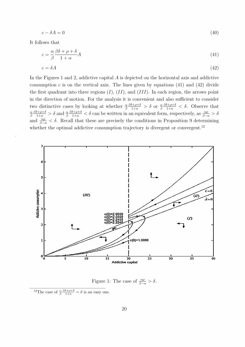
In the Figures 1 and 2, addictive capital A is depicted on the horizontal axis and addictive

consumption c is on the vertical axis. The lines given by equations (41) and (42) divide

the first quadrant into three regions (I), (II), and (III). In each region, the arrows point

in the direction of motion. For the analysis it is convenient and also sufficient to consider

two distinctive cases by looking at whether αββδ+ρ+δ1+α

> δ or αββδ+ρ+δ1+α

< δ. Observe thatαββδ+ρ+δ1+α

> δ and αββδ+ρ+δ1+α

< δ can be written in an equivalent form, respectively, as αρβ−α > δ

and αρβ−α < δ. Recall that these are precisely the conditions in Proposition 9 determining

whether the optimal addictive consumption trajectory is divergent or convergent.12

Figure 1: The case of αρβ−α > δ.

12The case of αβ

βδ+ρ+δ1+α = δ is an easy one.

20

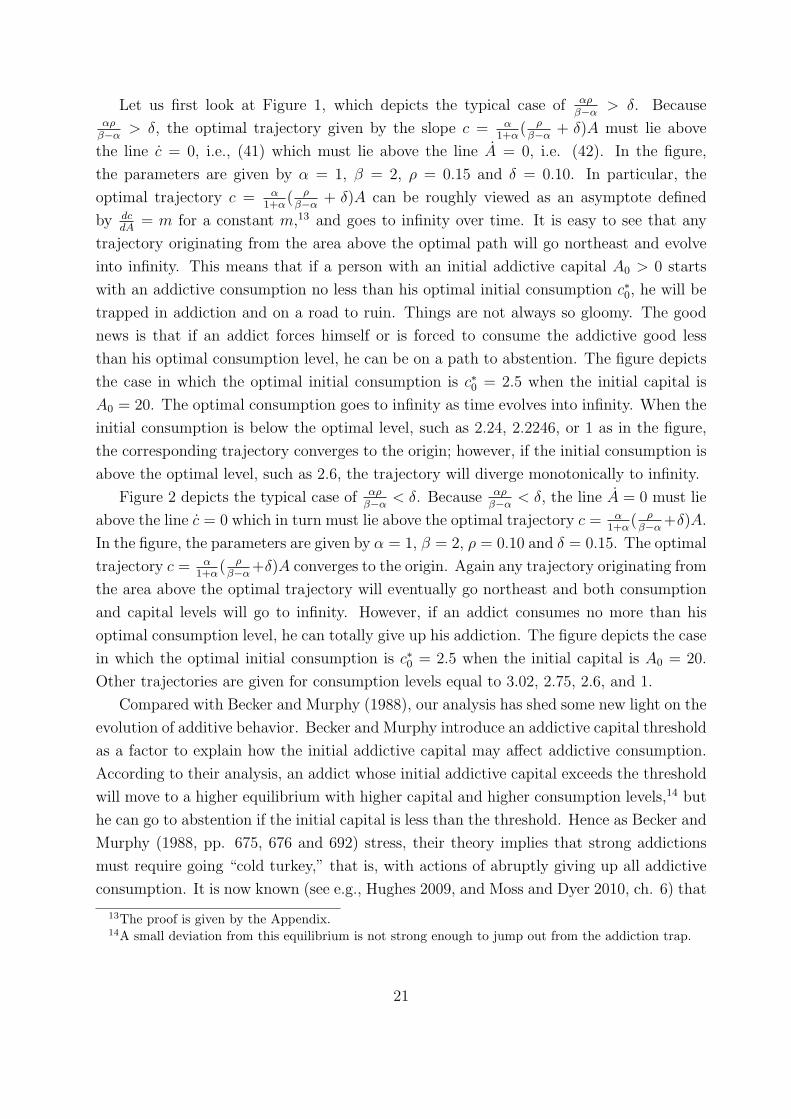
Let us first look at Figure 1, which depicts the typical case of αρβ−α > δ. Because

αρβ−α > δ, the optimal trajectory given by the slope c = α

1+α( ρβ−α + δ)A must lie above

the line c = 0, i.e., (41) which must lie above the line A = 0, i.e. (42). In the figure,

the parameters are given by α = 1, β = 2, ρ = 0.15 and δ = 0.10. In particular, the

optimal trajectory c = α1+α

( ρβ−α + δ)A can be roughly viewed as an asymptote defined

by dcdA

= m for a constant m,13 and goes to infinity over time. It is easy to see that any

trajectory originating from the area above the optimal path will go northeast and evolve

into infinity. This means that if a person with an initial addictive capital A0 > 0 starts

with an addictive consumption no less than his optimal initial consumption c∗0, he will be

trapped in addiction and on a road to ruin. Things are not always so gloomy. The good

news is that if an addict forces himself or is forced to consume the addictive good less

than his optimal consumption level, he can be on a path to abstention. The figure depicts

the case in which the optimal initial consumption is c∗0 = 2.5 when the initial capital is

A0 = 20. The optimal consumption goes to infinity as time evolves into infinity. When the

initial consumption is below the optimal level, such as 2.24, 2.2246, or 1 as in the figure,

the corresponding trajectory converges to the origin; however, if the initial consumption is

above the optimal level, such as 2.6, the trajectory will diverge monotonically to infinity.

Figure 2 depicts the typical case of αρβ−α < δ. Because αρ

β−α < δ, the line A = 0 must lie

above the line c = 0 which in turn must lie above the optimal trajectory c = α1+α

( ρβ−α+δ)A.

In the figure, the parameters are given by α = 1, β = 2, ρ = 0.10 and δ = 0.15. The optimal

trajectory c = α1+α

( ρβ−α+δ)A converges to the origin. Again any trajectory originating from

the area above the optimal trajectory will eventually go northeast and both consumption

and capital levels will go to infinity. However, if an addict consumes no more than his

optimal consumption level, he can totally give up his addiction. The figure depicts the case

in which the optimal initial consumption is c∗0 = 2.5 when the initial capital is A0 = 20.

Other trajectories are given for consumption levels equal to 3.02, 2.75, 2.6, and 1.

Compared with Becker and Murphy (1988), our analysis has shed some new light on the

evolution of additive behavior. Becker and Murphy introduce an addictive capital threshold

as a factor to explain how the initial addictive capital may affect addictive consumption.

According to their analysis, an addict whose initial addictive capital exceeds the threshold

will move to a higher equilibrium with higher capital and higher consumption levels,14 but

he can go to abstention if the initial capital is less than the threshold. Hence as Becker and

Murphy (1988, pp. 675, 676 and 692) stress, their theory implies that strong addictions

must require going “cold turkey,” that is, with actions of abruptly giving up all addictive

consumption. It is now known (see e.g., Hughes 2009, and Moss and Dyer 2010, ch. 6) that

13The proof is given by the Appendix.14A small deviation from this equilibrium is not strong enough to jump out from the addiction trap.

21

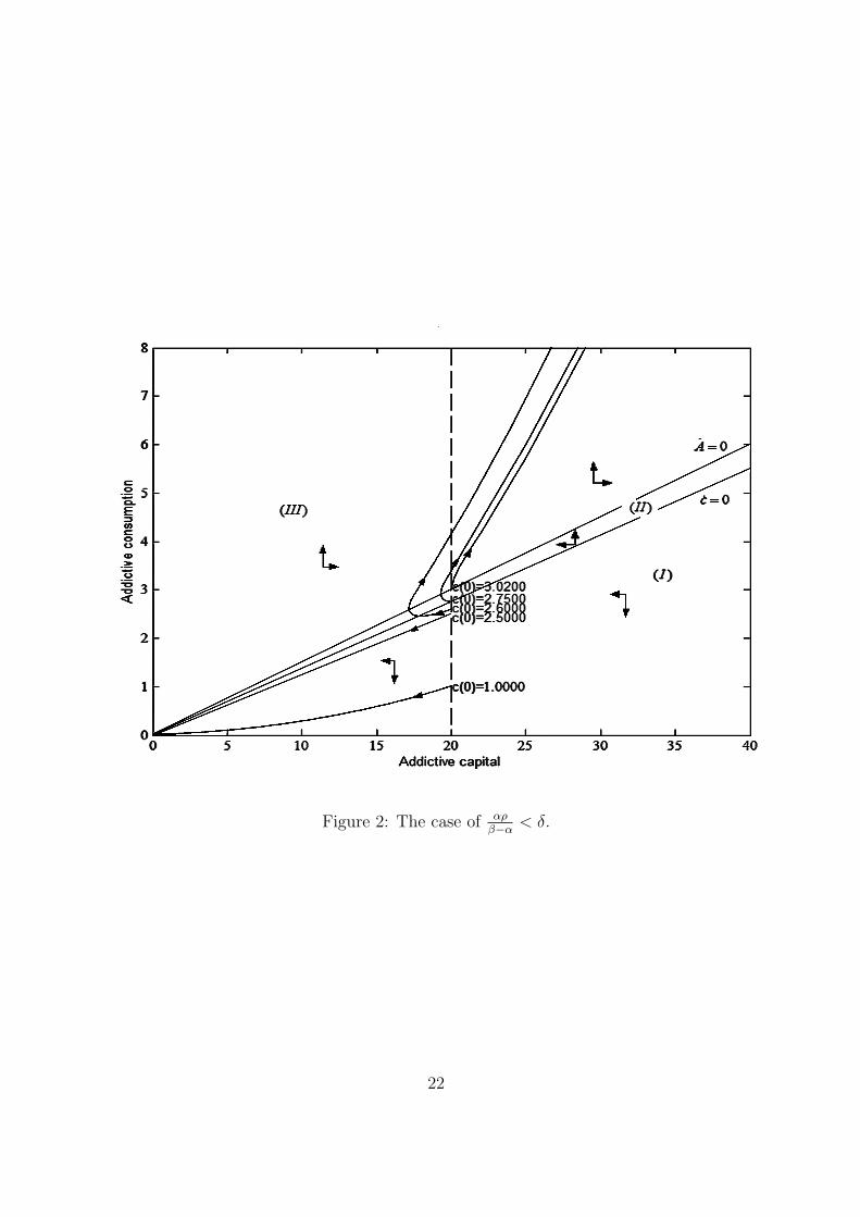
Figure 2: The case of αρβ−α < δ.

22

cold turkey is not an appropriate treatment for breaking certain addictions, because going

cold turkey can cause immense withdrawal syndrome potentially resulting in death. For

instance, treating alcoholics with this method can trigger life-threatening delirium tremens.

In general, going cold turkey, even if not life-threatening, can be still extremely unpleasant

or painful for most people, because of severe withdrawal effect. Notice that even if an

addict goes cold turkey meaning that he immediately quits or dramatically reduces his

addictive consumption, his addictive capital, however, cannot immediately disappear or

decrease substantially. Instead it will decrease only gradually, meaning that the painful

period might not be short.

Our analysis above offers fresh hope that there does exist a soft treatment-a less painful

but gradual reduction process for ending addiction, no matter how long or how seriously a

person has become addicted, as long as he has a will or is slightly forced to consume (even

just a little bit) less than his optimal addictive consumption level. Policy implications from

our analysis are that in order to achieve addiction abstention, one can use soft treatment,

or harsh treatment-cold turkey, or both. For instance, if a person has severe withdrawal

symptoms, he can initially use soft treatment until he reaches a tolerable level from which

cold turkey could be explored to terminate addictions once and for all. One caveat is that

our analysis in this section has so far ignored uncertainty. In stochastic environments, even

if a person currently stays in a safe zone, that is, his trajectory lies below his optimal path,

random events may easily trigger him to consume more than his optimal consumption

level and thus drive him into a dangerous zone. This suggests that addiction control is a

complex process and requires extreme caution and constant care in order to stop addiction

and prevent its relapse.

4.2 Analytical Solutions of ODE with General Initial Values

In this subsection we examine how initial addictive consumption c0 and capital A0 affect

evolution of addictive behavior. In the optimal control problem (29), c is a control variable

and A0 is the only given initial condition. The goal was to find the optimal consumption

path c(t) for all t ≥ 0. Now we ask a different but relevant question: given any initial

values c0 and A0, how c(t) and A(t) will evolve over time. To provide quantitative answers,

we need to solve the following system of ordinary differential equations (ODE):

c =c2

α(α + 1)A[αβ

c(c− δA)− (ρ+ δ)

αA

c+ β], c(0) = c0 (43)

A = c− δA, A(0) = A0 (44)

Let m1 =1

1+α(βδ + ρ+ δ)− δ and m2 =

β−αα

. Recall that η = α1+α

( ρβ−α + δ). Observe that

η = m1

m2. We can establish the following theorem whose proof is given in the Appendices I

23

and J.

Theorem 2 The solutions to (43) and (44) are

A(t) = A0[A0

c0em1t

1η+ em1t(A0

c0− 1

η)]

1m2 e−δt (45)

c(t) =1

1η+ em1t(A0

c0− 1

η)A(t) (46)

It is easy to verify that substituting c0 =α

1+α( ρβ−α+δ)A0 into (45) and (46) yields the same

optimal solution as given by (36). Let c∗0 denote the optimal consumption α1+α

( ρβ−α + δ)A0.

Using (45) and (46) we can derive the following two results.

Proposition 14 In the case of αρβ−α > δ, both the optimal addictive capital and optimal

addictive consumption are increasing functions of time, that is, A(t) and c(t) are given by

(45) and (46) with c0 = ηA0 > 0. The trajectories (A(t), c(t)) given by (45) and (46) with

c0 > ηA0 are also increasing functions of time and will finally diverge to infinity, whereas

the trajectories (A(t), c(t)) given by (45) and (46) with c0 < ηA0 will be decreasing after a

period of time and converge to the origin.

Proposition 15 In the case of αρβ−α < δ, both the optimal addictive capital and optimal

addictive consumption are decreasing functions of time and converge to the origin, that is,

A(t) and c(t) are given by (45) and (46) with c0 = ηA0 > 0. The trajectories (A(t), c(t))

given by (45) and (46) with c0 < ηA0 are also decreasing functions of time and will converge

to the origin, whereas the trajectories (A(t), c(t)) given by (45) and (46) with c0 > ηA0 will

be increasing after a period of time and finally diverge to infinity.

From (45) and (46), we can see that both A(t) and c(t) are positive for all t > 0 ifA0

c0− 1

η> 0. Notice that A0

c0− 1

η> 0 is equivalent to c0 < ηA0, i.e., the initial values are

inside the stable area characterized by the line of optimal solution c = ηA. What is the

property of trajectories originating above the line of c = ηA? From Figures 1 and 2, it

appears that the trajectories will diverge to infinity as t→ ∞. In fact, it is easy to calculate

from (45) and (46) that both A(t) and c(t) can rise to any substantially high level within

a relatively short period of time t∗ = − 1m1

ln εη+ε

(see the Appendix for its computation).

This means that once an addict enters the unstable zone, his addictive consumption can

easily spiral out of control. This phenomenon is consistent with behaviors of addicts of

many powerful substances such as opium and heroin.

We now investigate how initial values A0 and c0 influence a person’s total utility. By

substituting (45) and (46) into the objective function∫∞0

− (A(t))β

(c(t))αe−ρtdt, we obtain the total

value of utility

J(A0, c0) = −Aβ0

cα0

1 + α

ρ+ (β − α)δ

24

Proposition 16 For any 0 < c0 ≤ c∗0, we have ∂J(A0,c0)∂c0

=Aβ0cα+10

α(1+α)ρ+(β−α)δ > 0, ∂2J(A0,c0)

∂c0∂A0=

Aβ−10

cα+10

αβ(1+α)ρ+(β−α)δ > 0, and ∂J(A0,c0)

∂A0= −Aβ−1

0

cα0

β(1+α)ρ+(β−α)δ < 0

The first inequality says that the marginal utility of initial addictive consumption c0 is

positive. This means that a utility maximizer will try to raise his initial consumption c0

so as to increase his total utility J(A0, c0). The second inequality states that the marginal

utility of initial addictive consumption is an increasing function of initial capital A0. That

is, higher initial addictive capital A0 will induce the agent to consume more addictive good.

As a result, it will become more difficult to give up his addiction. For example, smoking is

harder to give up for those who have a long smoking history and a high addictive capital

than for those who have a short history and a low capital. The last inequality means that

the marginal utility of initial addictive capital A0 is negative. That is to say, the person

would be quite happy to reduce his initial capital, should it be possible for him to do so. We

should, however, keep in mind that an addict cannot directly control his addictive capital

being a state variable, and he can only influence his addictive capital by managing his

addictive consumption being a control variable. Because of the second relation, lowering

capital A0 will also lower consumption c0. The three inequalities give a mixed message

about addiction control. A final point is that even with the same initial addictive A0, the

difficulty of addiction control varies from person to person, because each person’s utility

depends on his personal factors α, β, ρ, and δ.

5 Conclusion

Addictions are fundamental and perplexing types of human behavior, and are extremely

difficult to model because of their unique and mysterious nature. In a path-breaking pa-

per, Becker and Murphy (1988) develop a general rational choice framework for studying

the dynamic behavior of addictive consumption. They model addictions in a determinis-

tic environment as habit formation by capturing three fundamental features of addictive

behavior: tolerance, withdrawal and reinforcement. The theoretical and empirical insights

provided by Becker and Murphy (1988) and many subsequent studies have considerably

advanced our understanding of addiction and also influenced decision makers on addiction

control policy.

The current paper has developed a more realistic rational addiction framework that not

only maintains the essential features of the Becker-Murphy model: tolerance, withdrawal

and reinforcement, but also takes a crucial factor –uncertainty– that addicts have to face

more often than nonaddicts do, into consideration. It is widely observed that random

events such as divorce, unemployment, death of a loved one, peer pressure, exposure to

25

environmental cues, etc, can precipitate and exacerbate an addiction, while sober and

thought-provoking events such as the death of a friend caused by addiction and compelling

campaigns against drugs, can discourage addiction. In our new framework uncertainty

is modeled through the Wiener stochastic process. Somewhat surprisingly we have been

able to derive closed-form expressions for both the optimal and expected optimal addictive

consumption and capital trajectories. These solutions enable us to derive both global and

local, qualitative and quantitative, properties of dynamic addictive behavior.

Our results explain several typical patterns of addictive behavior including cycles of

binges and abstention attempts, and also have novel implications for addiction control pol-

icy. For instance, in contrast to the theory of Becker and Murphy implying that cold turkey

must be used to terminate severe addictions, our theory offers an alternative approach-a

soft treatment. That is, we demonstrate that there always exists a gradual and less painful

process for ending addiction. We believe this insight is both important and practical for

policy implementation, because harsh treatment-like going cold turkey can be extremely

dangerous or even life-threatening. To achieve addiction abstention, our theory permits a

flexible and comprehensive approach: the use of soft treatment, or harsh treatment, or a

combination of both.

In our analysis, we have made good use of the addictive multivariate power utility

functions that not only capture three basic characteristics of addictive behavior: tolerance,

withdrawal and reinforcement, but also admit intuitive interpretations and facilitate the

analysis. Becker and Murphy (1988) first propose general conditions that meet the three

basic characteristics of addictive behavior and then use a quadratic utility function as an

approximation to carry out their analysis. In this way it is very difficult if not impossible

to derive global properties of dynamic addictive behavior. In fact, a number of subsequent

studies have also explored similar quadratic functions as an approximation. The great

advantage of the addictive multivariate power utility function is that it dispenses with the

approximation, admits natural and meaningful interpretations, and more importantly it

helps to achieve explicit solutions and therefore permits us to gain clear insights. Even in

the deterministic case, we also obtain substantial new results that go beyond the existing

ones.

The current study also leaves us with some open questions. For the purpose of treat-

ment and prevention of addiction, it would be a great advance if scientists could invent a

device or method to detect and gauge the level of addictive capital in the human body.

Recall that reinforcement, tolerance and withdrawal are part of the widely accepted and

observed syndrome of addiction. The rational models of Becker and Murphy and sub-

sequent researchers have well captured these fundamental features. It is our conjecture

that the ‘substance’ of the addictive capital should exist in an addictive human body. As

26

pointed out previously, because of the incorporation of uncertainty, we have ignored the

effect of a normal good in our analysis. It is, however, reasonable to expect that many

insights obtained in this article could carry over to the more general model with a normal

good. We believe that the analysis developed here for the basic model provides a useful and

necessary foundation for the study of the more general problem. How to solve the general

problem remains a challenge. Resolving this problem will yield a better understanding of

how pricing and/or taxing on the addictive good affects the addictive behavior.

References

[1] Adda, J., and Cornagia, F. “Taxes, cigarette consumption, and smoking intensity.”

American Economic Review 96 (2006), 1013-1028.

[2] Akerlof, G. A. “Procrastination and obedience.” (Papers and Proceedings) American

Economic Review 81 (1991), 1-19.

[3] Becker, G. S., and Murphy, K.M. “A theory of rational addiction.” Journal of Political

Economy 96 (1988), 675-700.

[4] Becker, G. S., and Murphy, K.M. “A simple theory of advertising as a good or a bad.”

Quarterly Journal of Economics CVIII (1988), 941-964.

[5] Becker, G. S., Grossman, M., and Murphy, K.M. “Rational addiction and the effect

of price on consumption.” (Papers and Proceedings) American Economic Review 81

(1991), 237-241.

[6] Becker, G. S., Grossman, M., and Murphy, K.M. “An empirical analysis of cigarette

addiction.” American Economic Review 84 (1994), 396-418.

[7] Bernheim, B.G., and Rangel, A. “Addiction and cue-triggered decision processes.”

American Economic Review 94 (2004), 1558-1590.

[8] Black, F., Scholes, M. “The pricing of options and corporate liabilities.” Journal of

Political Economy 81 (1973), 637-659.

[9] Carbone, J.C., Kverndokk, S., and Rogeberg, O. J. “Smoking, health, risk, and per-

ception.” Journal of Health Economics 24 (2005), 631-653.

[10] Chaloupka, F. “Rational addictive behavior and cigarette smoking.” Journal of Polit-

ical Economy 99 (1991), 722-742.

27

[11] Fenn, A.J., Antonovitz, F., and Schroeter, J. R. “Cigarettes and addiction information:

new evidence in support of the rational addiction model.” Economics Letters 72 (2001),

39-45.

[12] Fleming, W. H., Soner, H. M. Controlled Markov Processes and Viscosity Solutions,

2nd ed., Springer, New York, 2006.

[13] Goldstein, A. Addiction: From Biology to Drug Policy, 2nd ed., Oxford University

Press, New York, 2001.

[14] Grossman, M., and Chaloupka, F. “The demand for cocaine by young adults: a ratio-

nal addiction approach.” Journal of Health Economics 17 (1998), 427-474.

[15] Grossman, M., Chaloupka, F., and Sirtalan, I. “An empirical analysis of alcohol ad-

diction: results from the Monitoring the Future panels.” Economic Inquiry 36 (1998),

39-48.

[16] Gruber, J., and Koszegi, B. “Is addiction “rational”? theory and practice.” Quarterly

Journal of Economics 116 (2001), 1261-1303.

[17] Hughes, J. R. “Alcohol withdrawal seizures.” Epilepsy and Behavior 15 (2009), 92-97.

[18] Iannaccone, L. R. “Addiction and satiation.” Economics Letters 21 (1986), 95-99.

[19] Kamien, M. I., and Schwartz, N.L. Dynamic Otimization: The Calculus of Variations

and Optimal Control in Economics and Management. North-Holland, Amsterdam,

1991.

[20] Keeler, T.E., Hu, T., Barnett, P.G., and Manning, W.G.“Taxation, regulation, and

addiction: a demand function for cigarettes based on time-series evidence.” Journal

of Health Economics 12 (1993), 1-18.

[21] Laibson, D. “A cue-theory of consumption.” Quarterly Journal of Economics 116

(2001), 81-119.

[22] Merton, R.C. “Lifetime Portfolio Selection under Uncertainty: The Continuous-Time

Case.” The Review of Economics and Statistics 51 (1969), 247-257.

[23] Merton, R.C. “Optimum consumption and portfolio rules in a continuos-time model.”

Journal of Economic Theory 3 (1971), 373-413.

[24] Mirrlees, J. A. “Optimum Accumulation Under Uncertainty.” PhD Dissertation in

Economics, Cambridge University, 1963.

28

[25] Mobilia, P. An Economic Analysis of Addictive Behavior: The Case of Gambling, PhD

dissertation, City University of New York, 1990.

[26] Moss, A.C. and Dyer, K. R. Psychology of Addictive Behaviour, Palgrave MacMillan,

New York, 2010.

[27] Olekalns, N., and Bardsley, P. “Rational addiction to caffeine: an analysis of coffee

consumption.” Journal of Political Economy 104 (1996), 1100-1104.

[28] Orphanides, A., and Zervos, D. “Rational addiction with learning and regret.” Journal

of Political Economy 103 (1995), 739-758.

[29] Peele, S. The Meaning of Addiction: Compulsive Experience and Its Interpretation.

Lexington, Mass. 1985.

[30] Ryder, H. E. Jr., and Heal, G. M. “Optimum growth with intertemporally dependent

preferences.” Review of Economic Studies 40 (1973), 1-33.

[31] Schelling, T. C. “Self-command in practice, in policy, and in a theory of rational

choice.” (Papers and Proceedings) American Economic Review 74 (1984), 1-11.

[32] Sethi, S. P., and Thompson, G.L. Optimal Control Theory: Applications to Manage-

ment Science and Economics. Kluwer, 2nd Edition, 2000.

[33] Stigler, G.J., and Becker, G.S. “De Gustibus Non Est Disputandum.” American Eco-

nomic Review 67 (1977), 76-90.

[34] Suranovic, S. M., Goldfarb, R., and Leonard, T. C. “An economic theory of cigarette

addiction.” Journal of Health Economics 18 (1999), 1-29.

[35] Taylor, P. “Can the tobacco industry shed its ‘toxic brand’?”, May 29, 2014, BBC

report, http://www.bbc.co.uk/news/health-27546922.

[36] Vuchinich, R.V., and Heather, N. Choice, Behavioural Economics and Addiction, Perg-

amon, New York, eds, 2003.

[37] Weitzman, M. C. “Gamma discounting.” American Economic Review 91 (2001), 260-

271.

[38] West, R. Theory of Addiction, Blackwell, Oxford, 2006.

[39] Winston, G.C. “Addiction and backsliding: a theory of compulsive consumption.”

Journal of Economic Behavior and Organization 1 (1980), 295-324.

29

[40] World Health Organization. “Global status report on alcohol and health.”

http://www.who.int, 2011.

[41] World Health Organization. “WHO global report: mortality attributable to tobacco.”

http:// www.who.int, 2012.

[42] Yong, J. M., Zhou, X. Y. Stochastic Controls, Springer, New York, 1999.

Appendix

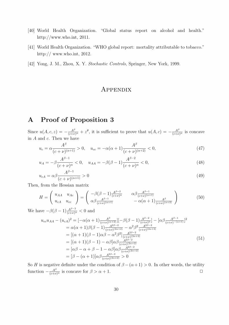
A Proof of Proposition 3

Since u(A, c, z) = − Aβ

(c+ν)α+ zθ, it is sufficient to prove that u(A, c) = − Aβ

(c+ν)αis concave

in A and c. Then we have

uc = αAβ

(c+ ν)(α+1)> 0, ucc = −α(α + 1)

Aβ

(c+ ν)(α+2)< 0, (47)

uA = −β Aβ−1

(c+ ν)α< 0, uAA = −β(β − 1)

Aβ−2

(c+ ν)α< 0, (48)

ucA = αβAβ−1

(c+ ν)(α+1)> 0 (49)

Then, from the Hessian matrix

H =

(uAA uAc

ucA ucc

)=

(−β(β − 1) Aβ−2

(c+ν)ααβ Aβ−1

(c+ν)(α+1)

αβ Aβ−1

(c+ν)(α+1) − α(α + 1) Aβ

(c+ν)(α+2)

)(50)

We have −β(β − 1) Aβ−2

(c+ν)α< 0 and

uccuAA − (ucA)2 = [−α(α + 1) Aβ

(c+ν)(α+2) ][−β(β − 1) Aβ−2

(c+ν)α]− [αβ Aβ−1

(c+ν)−(α+1) ]2

= α(α + 1)β(β − 1) A2β−2

(c+ν)(2α+2) − α2β2 A2β−2

(c+ν)(2α+2)

= [(α + 1)(β − 1)αβ − α2β2] A2β−2

(c+ν)(2α+2)

= [(α + 1)(β − 1)− αβ]αβ A2β−2

(c+ν)(2α+2)

= [αβ − α + β − 1− αβ]αβ A2β−2

(c+ν)(2α+2)

= [β − (α + 1)]αβ A2β−2

(c+ν)(2α+2) > 0

(51)

So H is negative definite under the condition of β− (α+1) > 0. In other words, the utility

function − Aβ

(c+ν)αis concave for β > α + 1. 2

30

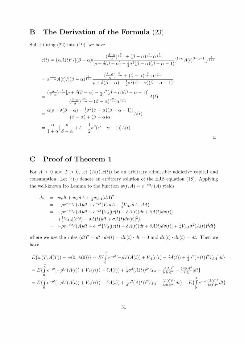
B The Derivation of the Formula (23)

Substituting (22) into (19), we have

c(t) = {αA(t)β/[(β − α)((β−α

α)

α1+α + (β − α)

α1+αα

11+α

ρ+ δ(β − α)− 12σ2(β − α)(β − α− 1)

)1+αA(t)β−α−1]}1

1+α

= α1

1+αA(t)/[(β − α)1

1+α(β−α

α)

α1+α + (β − α)

α1+αα

11+α

ρ+ δ(β − α)− 12σ2(β − α)(β − α− 1)

]

=( αβ−α)

11+α [ρ+ δ(β − α)− 1

2σ2(β − α)(β − α− 1)]

(β−αα

)α

1+α + (β − α)α

1+αα1

1+α

A(t)

=α[ρ+ δ(β − α)− 1

2σ2(β − α)(β − α− 1)]

(β − α) + (β − α)αA(t)

=α

1 + α[

ρ

β − α+ δ − 1

2σ2(β − α− 1)]A(t)

2

C Proof of Theorem 1

For A > 0 and T > 0, let (A(t), c(t)) be an arbitrary admissible addictive capital and

consumption. Let V (·) denote an arbitrary solution of the HJB equation (18). Applying

the well-known Ito Lemma to the function w(t, A) = e−ρtV (A) yields

dw = wtdt+ wAdA+ 12wAA(dA)

2

= −ρe−ρtV (A)dt+ e−ρt(VAdA+ 12VAAdA · dA)

= −ρe−ρtV (A)dt+ e−ρt{VA[(c(t)− δA(t))dt+ δA(t)dv(t)]

+12VAA[(c(t)− δA(t))dt+ σA(t)dv(t)]2}

= −ρe−ρtV (A)dt+ e−ρt{VA[(c(t)− δA(t))dt+ δA(t)dv(t)] + 12VAAσ

2(A(t))2dt}

where we use the rules (dt)2 = dt · dv(t) = dv(t) · dt = 0 and dv(t) · dv(t) = dt. Then we

have

E{w(T,A(T ))− w(0, A(0))} = E{T∫0

e−ρt[−ρV (A(t)) + VA(c(t)− δA(t)) + 12σ2(A(t))2VAA]dt}

= E{T∫0

e−ρt[−ρV (A(t)) + VA(c(t)− δA(t)) + 12σ2(A(t))2VAA + (A(t))β

(c(t))α− (A(t))β

(c(t))α]dt}

= E{T∫0

e−ρt[−ρV (A(t)) + VA(c(t)− δA(t)) + 12σ2(A(t))2VAA + (A(t))β

(c(t))α]dt} − E{

T∫0

e−ρt (A(t))β

(c(t))αdt}

31

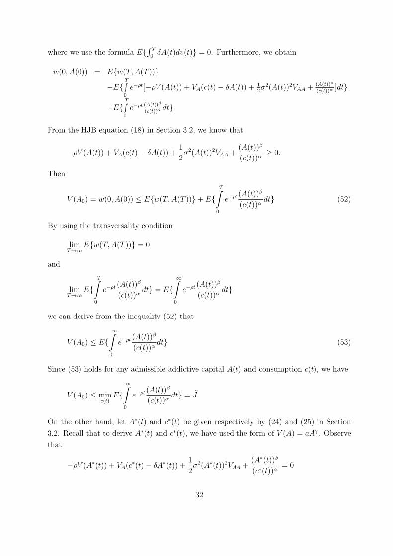
where we use the formula E{∫ T0δA(t)dv(t)} = 0. Furthermore, we obtain

w(0, A(0)) = E{w(T,A(T ))}

−E{T∫0

e−ρt[−ρV (A(t)) + VA(c(t)− δA(t)) + 12σ2(A(t))2VAA + (A(t))β

(c(t))α]dt}

+E{T∫0

e−ρt (A(t))β

(c(t))αdt}

From the HJB equation (18) in Section 3.2, we know that

−ρV (A(t)) + VA(c(t)− δA(t)) +1

2σ2(A(t))2VAA +

(A(t))β

(c(t))α≥ 0.

Then

V (A0) = w(0, A(0)) ≤ E{w(T,A(T ))}+ E{T∫

0

e−ρt(A(t))β

(c(t))αdt} (52)

By using the transversality condition

limT→∞

E{w(T,A(T ))} = 0

and

limT→∞

E{T∫

0

e−ρt(A(t))β

(c(t))αdt} = E{

∞∫0

e−ρt(A(t))β

(c(t))αdt}

we can derive from the inequality (52) that

V (A0) ≤ E{∞∫0

e−ρt(A(t))β

(c(t))αdt} (53)

Since (53) holds for any admissible addictive capital A(t) and consumption c(t), we have

V (A0) ≤ minc(t)

E{∞∫0

e−ρt(A(t))β

(c(t))αdt} = J

On the other hand, let A∗(t) and c∗(t) be given respectively by (24) and (25) in Section

3.2. Recall that to derive A∗(t) and c∗(t), we have used the form of V (A) = aAγ. Observe

that

−ρV (A∗(t)) + VA(c∗(t)− δA∗(t)) +

1

2σ2(A∗(t))2VAA +

(A∗(t))β

(c∗(t))α= 0

32

This means that the HJB equation is satisfied by (A(t), c(t)). Therefore,

V (A0) = w(0, A(0))

= E{w(T,A∗(T ))}+ E{T∫0

e−ρt (A∗(t))β

(c∗(t))αdt}

= E{e−ρTV (A∗(T ))}+ E{T∫0

e−ρt (A∗(t))β

(c∗(t))αdt}

It remains to show that limT→∞E{w(T,A∗(T ))} = 0. Notice that

limT→∞E{w(T,A∗(T ))} = limT→∞E{e−ρTaA∗(T )β−α}= limT→∞ aE{exp(−ρT )Aβ−α0 exp{[ α

1+α( ρβ−α − 1

2σ2(β − α− 1))

− δ1+α

− σ2

2]T + σv(T )}β−α}

= limT→∞ aAβ−α0 E{exp{−ρT + (β − α)[ α1+α

( ρβ−α

−12σ2(β − α− 1))− δ

1+α− σ2

2]T + σ(β − α)v(T )}}

= limT→∞ aAβ−α0 exp{−(β − α)[ ρ+δ1+α

+ α2(1+α)

σ2(β − α− 1)]T}= 0

Then we have

V (A0) = limT→∞E{T∫0

e−ρt (A∗(t))β

(c∗(t))αdt}

= E{∞∫0

e−ρt (A∗(t))β

(c∗(t))αdt}

≥ minE{∞∫0

e−ρt (A(t))β

(c(t))αdt}

= J

(54)

By (53) and (54), V (A0) = J . 2

D Proof of Proposition 5

We prove ∂c∂ψ

< 0. The same argument works for ∂E{c}∂ψ

< 0. Plugging ψ = β − α into c(t)

of (25) yields

c(t) = A0(β − ψ

1 + β − ψ)(ρ

ψ+ δ − 1

2σ2(ψ − 1))e{[(

β−ψ1+β−ψ )( ρ

ψ+δ− 1

2σ2(ψ−1))−δ−σ2

2]t+σv(t)}.

Then we have

∂c∂ψ

= A0[−1

(1+β−ψ)2 (ρψ+ δ − σ2

2(ψ − 1)) + β−ψ

1+β−ψ (−ρψ2 − σ2

2)](1 + ηt)e[(η−δ−

σ2

2)t+σv(t)]

= −A0[η

α(1+α)+ α

(1+α)2( ρ(β−α)2 +

σ2

2)](1 + ηt)e[(η−δ−

σ2

2)t+σv(t)]

< 0

as long as α > 0, η > 0 and t ≥ 0. 2

33

E The Optimal Solution of the Case of σ = 0

Consider the system of equations:

c =c

α(1 + α)A[αβ(c− δA)− α(ρ+ δ)A+ βc] (55)

A = c− δA, A(0) = A0 (56)

We guess the optimal addictive consumption is a linear function of addictive capital,

i.e. c(t) = ηA(t), where η is a positive constant to be determined. Substituting it into (56)

leads to

A = ηA− δA = (η − δ)A, A(0) = A0 (57)

Solving (57) for A(t) yields

A(t) = A0e(η−δ)t (58)

Then

c(t) = ηA(t) = ηA0e(η−δ)t (59)

Substituting (58) and (59) into RHS of (55) leads to

cα(1+α)A

[αβ(c− δA)− α(ρ+ δ)A+ βc]

= ηA0e(η−δ)t

α(1+α)A0e(η−δ)t[αβ(ηA0e

(η−δ)t − δA0e(η−δ)t)− α(ρ+ δ)A0e

(η−δ)t + βηA0e(η−δ)t]

= ηα(1+α)

[αβ(η − δ)− α(ρ+ δ) + βη]A0e(η−δ)t

(60)

Recall that c(t) = η(η − δ)A0e(η−δ)t by (58). Similarly, substituting it into LHS of (55)

gives

c(t) = η(η − δ)A0e(η−δ)t (61)

With the help of (55), (60), and (61), we have

η(η − δ)A0e(η−δ)t =

η

α(1 + α)[αβ(η − δ)− α(ρ+ δ) + βη]A0e

(η−δ)t (62)

34

From (62) we have

η = 1α(1+α)

[αβ(η − αβ)− α(ρ+ δ) + βη] + δ

= αβ+βα(1+α)

η − 1α(1+α)

[αβδ + α(ρ+ δ)] + δ

= βαη − 1

1+α(βδ + ρ+ δ) + δ

(63)

Then

(β

α− 1)η =

1

1 + α(βδ + ρ+ δ)− δ (64)

Solving for η in (64), we have

η = αβ−α [

11+α

(βδ + ρ+ δ)− δ] = αβ−α(

βδ1+α

+ ρ1+α

+ δ1+α

− δ)

= αβ−α(

βδ1+α

+ ρ1+α

− αδ1+α

)

= αβ−α [

(β−α)δ1+α

+ ρ1+α

]

= α1+α

( ρβ−α + δ)

(65)

Notice that η is identical to η if we set σ = 0 in the expression of η. In the meantime, it

is not hard to check the transversality condition limt→∞ λ(t)A(t)e−ρt = 0; see the following

Appendix.

By Proposition 13, the solution is a global optimal solution. 2

F Proof of the Transversality Condition (34)

Recall from (32) that

λ(t) = −α A(t)β

c(t)α+1(66)

Substituting (66) into limt→∞ λ(t)A(t)e−ρt leads to

limt→∞

λ(t)A(t)e−ρt = − limt→∞

αA(t)β

c(t)α+1A(t)e−ρt (67)

Substituting (58) and (59) into (67), we obtain

limt→∞

αA(t)β

c(t)α+1A(t)e−ρt = lim

t→∞αηα+1[A0e

(η−δ)t]β−αe−ρt (68)

35

Then

limt→∞ αηα+1[A0e(η−δ)t]β−αe−ρt = limt→∞ αηα+1Aβ−α0 e(β−α)(η−δ)te−ρt

= limt→∞ α[ α1+α

( ρβ−α + δ)]α+1Aβ−α0 e(β−α)[

α1+α

( ρβ−α+δ)−δ]te−ρt

= limt→∞ α[ α1+α

( ρβ−α + δ)]α+1Aβ−α0 e{

α1+α

[ρ+(β−α)δ]−(β−α)δ}te−ρt

= limt→∞ α[ α1+α

( ρβ−α + δ)]α+1Aβ−α0 e−

11+α

[ρ+(β−α)δ]t = 0

(69)

With the help of (67)-(69), we have limt→∞ λ(t)A(t)e−ρt = 0. 2

We also provide a second method of proving the above result. The method will be

referred in a later result.

From (67), we have

limt→∞

αA(t)β

c(t)α+1A(t)e−ρt = α lim

t→∞

A(t)β

c(t)αA(t)

c(t)e−ρt (70)

Combing this with (103) leads to

limt→∞

A(t)β

c(t)αA(t)

c(t)e−ρt = lim

t→∞Aβ−α0 (

A0

c0)αe−

11+α

[ρ+(β−α)δ]tA(t)

c(t)dt (71)

Substituting (97) into (71), we have

limt→∞Aβ−α0 (A0

c0)αe−

11+α

[ρ+(β−α)δ]t A(t)c(t)

= limt→∞Aβ−α0 (A0

c0)αe−

11+α

[ρ+(β−α)δ]t[ 1η+ em1t(A0

c0− 1

η)]

= limt→∞Aβ−α0 (A0

c0)αe−m1t[ 1

η+ em1t(A0

c0− 1

η)]

= limt→∞Aβ−α0 (A0

c0)α( 1

ηe−m1t + A0

c0− 1

η)

(72)

Obviously, c0 must be equal to ηA0, i.e.,A0

c0= 1

η, in order for the RHS of (72) to be

zero. 2

G Concavity of H0(t, A, λ)

The second order derivative of the maximized Hamiltonian function H0(t, λ, A) of (38) is

given by

∂H20

∂A2= −

βα+1

( βα+1

− 1)Aβα+1

−2

( α−λ)

αα+1

+ λ[(α

−λ)

1α+1

β

α + 1(

β

α + 1− 1)A

βα+1

−2] (73)

36

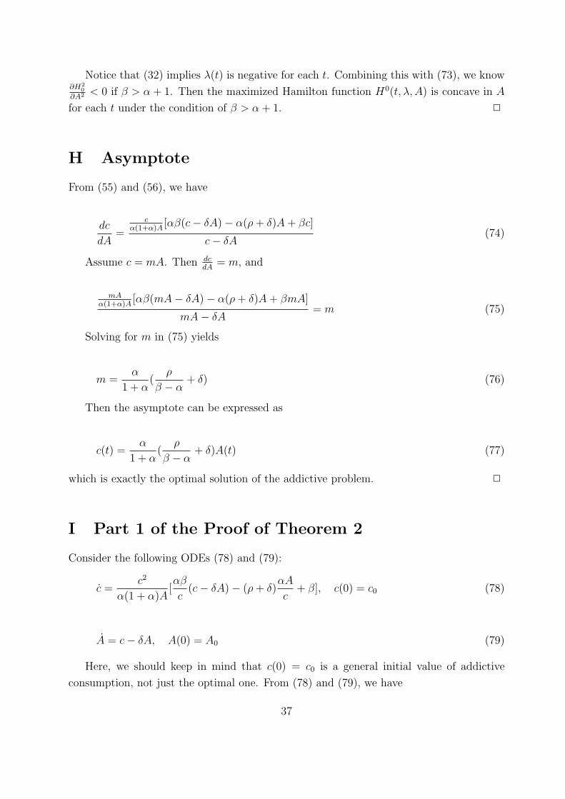
Notice that (32) implies λ(t) is negative for each t. Combining this with (73), we know∂H2

0

∂A2 < 0 if β > α + 1. Then the maximized Hamilton function H0(t, λ, A) is concave in A

for each t under the condition of β > α + 1. 2

H Asymptote

From (55) and (56), we have

dc

dA=

cα(1+α)A

[αβ(c− δA)− α(ρ+ δ)A+ βc]

c− δA(74)

Assume c = mA. Then dcdA

= m, and

mAα(1+α)A

[αβ(mA− δA)− α(ρ+ δ)A+ βmA]

mA− δA= m (75)

Solving for m in (75) yields

m =α

1 + α(

ρ

β − α+ δ) (76)

Then the asymptote can be expressed as

c(t) =α

1 + α(

ρ

β − α+ δ)A(t) (77)

which is exactly the optimal solution of the addictive problem. 2

I Part 1 of the Proof of Theorem 2

Consider the following ODEs (78) and (79):

c =c2

α(1 + α)A[αβ

c(c− δA)− (ρ+ δ)

αA

c+ β], c(0) = c0 (78)

A = c− δA, A(0) = A0 (79)

Here, we should keep in mind that c(0) = c0 is a general initial value of addictive

consumption, not just the optimal one. From (78) and (79), we have

37

cc= 1

α(1+α)cA[αβ(1− δA

c)− α(ρ+ δ)A

c+ β]

= 1α(1+α)

cA{αβ + β − [αβδ + α(ρ+ δ)]A

c}

= 1α(1+α)

{(αβ + β) cA− [αβδ + α(ρ+ δ)]}

= { 1α(1+α)

(αβ + β) cA− 1

α(1+α)[αβδ + α(ρ+ δ)]}

= [βαcA− 1

1+α(βδ + ρ+ δ)]

(80)

and

A

A=

c

A− δ (81)

Let c(t)A(t)

= y(t). Then we have c(t) = A(t)y(t) and cc= A

A+ y

y. Substituting them into

(80) and (81) leads to

y

y=β

αy − 1

1 + α(βδ + ρ+ δ)− A

A(82)

A

A= y − δ (83)

Substituting (83) into (82), we have

yy= β

αy − 1

1+α(βδ + ρ+ δ)− (y − δ)

= β−ααy + δ − 1

1+α(βδ + ρ+ δ)

(84)

Then

y = [δ − 1

1 + α(βδ + ρ+ δ)]y +

β − α

αy2 (85)

Notice that (85) is a Bernoulli equation. It can be changed into the following linear

ODE after a transformation of z(t) = 1y(t)

.

z = [1

1 + α(βδ + ρ+ δ)− δ]z − β − α

α(86)

Denote 11+α

(βδ + ρ+ δ)− δ and β−αα

by m1 and m2, respectively. Then (86) becomes

38

z = m1z −m2, z(0) = z0 (87)

Then its solution is

z(t) = em1t(z0 −∫ t

0

e−m1sm2ds) = em1t[z0 +m2

m1

(e−m1t − 1)] (88)

Notice the initial value z0 =1y(0)

= 1c(0)/A(0)

= A0

c0. Then

z(t) = em1t[A0

c0+m2

m1

(e−m1t − 1)] (89)

Then

c

A= y(t) =

1

z(t)=

1

em1t[A0

c0+ m2

m1(e−m1t − 1)]

(90)

Substituting (90) into (83) yields

A

A=

1

em1t[A0

c0+ m2

m1(e−m1t − 1)]

− δ (91)

Solving (91), we have (see the next Appendix for the computation detail)

A(t) = A0{em1t[1 + m2

m1/(A0

c0− m2

m1)]

em1t + m2

m1/(A0

c0− m2

m1)}

1m2 e−δt = A0{

A0

c0em1t

m2

m1+ em1t(A0

c0− m2

m1)}

1m2 e−δt (92)

If we let c0 = ηA0 =α

1+α( ρβ−α + δ)A0, i.e.,

A0

c0=

1α

1+α( ρβ−α + δ)

(93)

Noticing the definitions of m1 and m2, we have

m2

m1=

β−αα

11+α

(βδ+ρ+δ)−δ =β−αα

βδ+ρ+δ−(1+α)δ1+α

=β−αα

(β−α)δ+ρ1+α

= 1α

1+α(β−α)δ+ρβ−α

= 1α

1+α( ρβ−α+δ)

= 1η= A0

c0

(94)

39

Substituting (94) into (92) leads to

A(t) = A0(em1t)

1m2 e−δt = A0e

(η−δ)t (95)

Obviously, it is exactly the expression for the optimal addictive capital. By m2

m1= 1

η,

the general solution for addictive capital and (90) can be rewritten as

A(t) = A0[A0

c0em1t

1η+ em1t(A0

c0− 1

η)]

1m2 e−δt (96)

c(t)

A(t)=

1

em1t[A0

c0+ 1

η(e−m1t − 1)]

=1

1η+ em1t(A0

c0− 1

η)

(97)

Then

c(t) = A(t)c(t)

A(t)= A0[

A0

c0em1t

1η+ em1t(A0

c0− 1

η)]

1m2

11η+ em1t(A0

c0− 1

η)e−δt (98)

J Part II of the Proof of Theorem 2

Let lnA(t) = w(t). Then w(0) = w0 = lnA0,AA= w and (91) becomes

w =1

em1t[A(0)c(0)

+ m2

m1(e−m1t − 1)]

− δ (99)

Then

w(t) = w0 +t∫0

{ 1

em1s[A0c0

+m2m1

(e−m1s−1)]− δ}dt

= w0 +t∫0

1

em1s[A0c0

+m2m1

(e−m1s−1)]dt− δt

= w0 +t∫0

1

(A0c0

−m2m1

)em1s+m2m1

dt− δt

= w0 +t∫0

1h1em1s+h2

dt− δt

(100)

In the last line of (100), we have already assumed h1 =A0

c0− m2

m1and h2 =

m2

m1. Further,

let x(t) = em1t. Then t = 1m1

lnx and dt = 1m1

1xdx. Substituting them into (100) gives

40

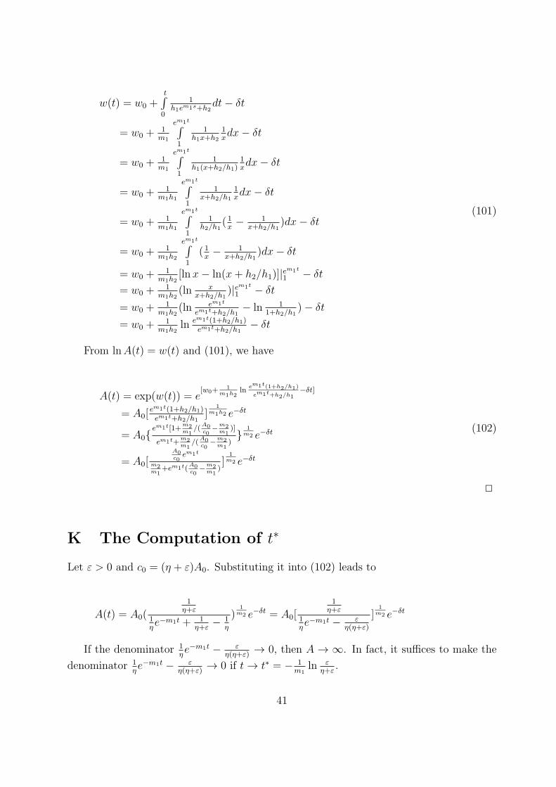
w(t) = w0 +t∫0

1h1em1s+h2

dt− δt

= w0 +1m1

em1t∫1

1h1x+h2

1xdx− δt

= w0 +1m1

em1t∫1

1h1(x+h2/h1)

1xdx− δt

= w0 +1

m1h1

em1t∫1

1x+h2/h1

1xdx− δt

= w0 +1

m1h1

em1t∫1

1h2/h1

( 1x− 1

x+h2/h1)dx− δt

= w0 +1

m1h2

em1t∫1

( 1x− 1

x+h2/h1)dx− δt

= w0 +1

m1h2[lnx− ln(x+ h2/h1)]|e

m1t

1 − δt

= w0 +1

m1h2(ln x

x+h2/h1)|em1t

1 − δt

= w0 +1

m1h2(ln em1t

em1t+h2/h1− ln 1

1+h2/h1)− δt

= w0 +1

m1h2ln em1t(1+h2/h1)

em1t+h2/h1− δt

(101)

From lnA(t) = w(t) and (101), we have

A(t) = exp(w(t)) = e[w0+

1m1h2

lnem1t(1+h2/h1)

em1t+h2/h1−δt]

= A0[em1t(1+h2/h1)em1t+h2/h1

]1

m1h2 e−δt

= A0{em1t[1+

m2m1

/(A0c0

−m2m1

)]

em1t+m2m1

/(A0c0

−m2m1

)}

1m2 e−δt

= A0[A0c0em1t

m2m1

+em1t(A0c0

−m2m1

)]

1m2 e−δt

(102)

2

K The Computation of t∗

Let ε > 0 and c0 = (η + ε)A0. Substituting it into (102) leads to

A(t) = A0(

1η+ε

1ηe−m1t + 1

η+ε− 1

η

)1m2 e−δt = A0[

1η+ε

1ηe−m1t − ε

η(η+ε)

]1m2 e−δt

If the denominator 1ηe−m1t − ε

η(η+ε)→ 0, then A → ∞. In fact, it suffices to make the

denominator 1ηe−m1t − ε

η(η+ε)→ 0 if t→ t∗ = − 1

m1ln ε

η+ε.

41

L Objective Value∞∫0

−Aβ

cαe−ρtdt =

∞∫0

−Aα

cαAβ−αe−ρtdt

= −∞∫0

[ 1η+ em1t(A0

c0− 1

η)]α{A0[

A0c0em1t

1η+em1t(

A0c0

− 1η)]

1m2 e−δt}β−αe−ρtdt

= −∞∫0

Aβ−α0 [ 1η+ em1t(A0

c0− 1

η)]α[

A0c0em1t

1η+em1t(

A0c0

− 1η)]β−αm2 e−[(β−α)δ+ρ]tdt

= −∞∫0

Aβ−α0 [ 1η+ em1t(A0

c0− 1

η)]α[

A0c0em1t

1η+em1t(

A0c0

− 1η)]αe−[(β−α)δ+ρ]tdt

= −∞∫0

Aβ−α0 (A0

c0em1t)αe−[(β−α)δ+ρ]tdt

= −Aβ−α0 (A0

c0)α

∞∫0

eαm1te−[(β−α)δ+ρ]tdt

= −Aβ−α0 (A0

c0)α

∞∫0

e{α

1+α[(β−α)δ+ρ]−(β−α)δ+ρ}tdt

= −Aβ−α0 (A0

c0)α

∞∫0

e−1

1+α[ρ+(β−α)δ]tdt

= −Aβ−α0 (A0

c0)α 1+α

ρ+(β−α)δ

(103)

Recall that A0

c0= 1

ηcorresponds to the optimal initial condition. Substituting it into (103)

leads to

−Aβ−α0 (A0

c0)α 1+α

ρ+(β−α)δ

= −Aβ−α0 ( 1η)α 1+α

ρ+(β−α)δ

= −Aβ−α0 [ 1α

1+α( ρβ−α+δ)

]α 1+αρ+(β−α)δ

= −Aβ−α0(1+α)1+α

[ρ+(β−α)δ][α( ρβ−α+δ)]

α

= −Aβ−α0 { (1+α)

[ρ+(β−α)δ]1

1+α [α( ρβ−α+δ)]

α1+α

}1+α

= −Aβ−α0 { (1+α)

[ρ+(β−α)δ]1

1+α [αρ+(β−α)δβ−α ]

α1+α

}1+α

= −Aβ−α0 { (1+α)

αα

1+α [ρ+(β−α)δ]1

1+α [ρ+(β−α)δ]

(β−α)α

1+α

α1+α

}1+α

= −Aβ−α0 { (1+α)(β−α)α

1+α

αα

1+α [ρ+(β−α)δ]}1+α

= −Aβ−α0 { (1+α)(β−αα

)α

1+α

[ρ+(β−α)δ] }1+α

= −Aβ−α0 { (β−αα

)α

1+α +α(β−αα

)α

1+α

[ρ+(β−α)δ] }1+α

= −Aβ−α0 { (β−αα

)α

1+α +(β−α)α

1+α α1

1+α

[ρ+(β−α)δ] }1+α

(104)

(104) is identical to the one obtained by HJB method if we set σ = 0.

42