Journal of Environmental Economics and Management, 64(2): 169-182. 2012.

Disentangling Preferences and Expectations in Stated Preference Analysis with Respondent

Uncertainty: The Case of Invasive Species Prevention

Bill Provencher, corresponding author Professor Department of Agricultural and Applied Economics University of Wisconsin, Madison 427 Lorch St. Madison, WI 53706 (608) 262-9494 rwproven@wisc.edu

David J. Lewis Assistant Professor Department of Economics University of Puget Sound 1500 N. Warner St. Tacoma, WA 98416 (253) 879-3553 djlewis@pugetsound.edu

Kathryn Anderson Graduate Student Department of Sociology University of Wisconsin, Madison 1710 University Ave., Room 287 Madison, WI 53706 (608) 890-0337 kganderson@wisc.edu

Running Title: Preferences and Expectations in Stated Preference Analysis

9/26/2011

1

Acknowledgements: We received outstanding advice from the manuscript’s referees. We thank

Eric Horsch, Steven Chambers, and Kate Zipp for research assistance. We thank seminar

participants at the AERE sessions in the 2009 AAEA annual meeting for helpful comments.

Funding was provided by the National Science Foundation via the Long Term Ecological

Research Network—North Temperate Lakes Site and the program in Coupled Human and

Natural Systems, and by the University of Wisconsin Sea Grant.

2

Abstract

Contingent valuation typically involves presenting the respondent with a choice to pay for a

program intended to improve future outcomes, such as a program to place parcels into

conservation easement, or a program to manage an invasive species. Deducing from these data

the value of the good (or bad) at the core of the program—the welfare gain generated by a parcel

of conserved land, for instance, or the loss incurred by a species invasion—often is not possible

because respondent preferences are conflated with their expectations about future environmental

outcomes in the absence of the program. This paper formally demonstrates this conundrum in

the context of a standard contingent valuation survey, and examines the use of additional survey

data to resolve it. The application is to the prevention of lake invasions by Eurasian

Watermilfoil (Myriophyllum spicatum), an invasive aquatic plant that is present in many lakes in

the northern U.S. and Canada and a possible threat to many more. Respondents are shoreline

property owners on lakes without Eurasian Watermilfoil. The estimated per-property welfare

loss of a lake invasion is $30,550 for one model and $23,614 for another, both of which are in

reasonable agreement with estimates obtained from a recent hedonic analysis of Eurasian

Watermilfoil invasions in the study area (Horsch and Lewis 2009), and from a companion

contingent valuation survey of shoreline property owners on already-invaded lakes.

Key Words: Stated preferences, expectations, respondent uncertainty, contingent valuation,

species invasions

3

I. Introduction

Well-designed stated preference surveys often present respondents with a choice to pay

for a program to avoid unfavorable events, or to induce favorable events. Asking respondents

about their willingness to pay for a program to affect an event, rather than directly asking their

willingness to pay for the outcome, is preferred as a matter of presenting a realistic valuation

scenario, thereby minimizing so-called “hypothetical bias”. So, for instance, rather than asking

respondents about their willingness to pay to prevent the extinction of a species, respondents are

asked about their willingness to pay for a particular program intended to assure the species is

preserved. Instances of such program-focused valuation studies abound in the contingent

valuation literature, and cannot be enumerated here, though a sampling pertaining to

environmental valuation over the years ranges from the reduction of old growth timber harvests

to preserve the northern spotted owl (Rubin et al.1991), to a phosphorus reduction program to

improve water clarity (Stumborg et al. 2001), to the preservation of urban open space (Kovacs

and Larson 2008).

Deducing from these data the value of the event that is the focus of the program can be

problematic because expressions of willingness to pay for the program are conflated with

expectations about future outcomes in the absence of the program. With reference to our species

preservation example, respondents might place a low value on a preservation program not

because they place a low value on the species, but rather because they don’t believe the species

will become extinct in the absence of the program. The analyst can account for this by explicitly

stating in the survey the outcome in the absence of the program (“Without the program, species

X will become extinct in the next 5 years”), but this likely is not sufficient when the respondent

has alternative beliefs about—or alternative conflicting information on—the counterfactual

4

outcome for the environmental good in question. Perhaps the most salient example is

environmental damage due to climate change. In a 2010 posting on its website, The Nature

Conservancy reports that only 18% of Americans “strongly believe that climate change is real,

human-caused and harmful”.1 Clearly a contingent valuation survey concerning a program to

mitigate a particular environmental damage due to climate change cannot rely on assertions in

the survey of the damage to unfold in the absence of the program.

In many instances the analyst may find it perfectly acceptable to estimate only the net

benefit of the program developed in the contingent valuation scenario, but often the “core good”

that is the focus of the program is the true subject of the valuation analysis, and extracting the

value of this good from the valuation of the program—obtaining a “portable” value, in other

words—is important in benefit transfer and understanding the welfare implications of changes in

environmental policies and programs. If the analyst is truly interested in the welfare gain

associated with an environmental good, or the welfare loss associated with an environmental

bad, then it is critical to understand the respondent’s judgment about the outcomes in the absence

of the program. Although we suspect that this issue is well understood by analysts engaged in

nonmarket valuation, we know of no attempts in the environmental economics literature to

explicitly disentangle expectations and preferences. In a review of the contingent valuation

method, Boyle (2003) observes, “Physical descriptions of changes in resource conditions

frequently are not available. In this case, contingent valuation questions often are framed to

value the policy change. With vague or nonexistent information on the resource change, survey

respondents are left to their own assumptions regarding what the policy change will accomplish”

1 http://www.nature.org/initiatives/climatechange/features/art26253.html. Available as of July 31, 2010. Results are based on The American Climate Values Survey, an ecoAmerica project conducted by SRIC-BI, and sponsored by the Alliance for Climate Protection, the Department of Conservation of the State of California, NRDC, and The Nature Conservancy.

5

(p. 117).2 He concludes, “This issue really has not been directly and extensively addressed in the

contingent valuation literature and deserves more consideration” (p. 118).

Disentangling expectations and preferences is the primary motivation for the large and

growing literature on the measurement of subjective probability distributions. Good recent

surveys of the literature are presented in Manski (2004), Hurd (2009), and Delavande, Gine, and

McKenzie (2011). Hurd (2009) observes,

“The objective of a theoretical or empirical investigation into intertemporal choice is to estimate preferences…However, such an investigation requires information about the probability distribution that the decision-maker used in coming to his or her choices because choice outcomes can be explained either by preferences or by subjective probability distributions (Manski 2004).” (pg. 544).

The primary contribution of this paper is to formally examine the conflation of

expectations and preferences in contingent valuation experiments, and to argue that without

additional information, separately identifying expectations and preferences requires strong

assumptions and is unlikely to generate estimates that are robust to the specification of the

willingness to pay (WTP) function. We show that additional survey data can resolve the

identification problem, and for a particular class of events that are common in contingent

valuation studies—binary events such as the extinction of a species, the preservation of a parcel

of land, the invasion of a lake by a non-native species, and so forth—this resolution is especially

clean and cheap (in terms of the data requirement), though it does require parametric

assumptions about how the respondent’s subjective probability of an event evolves over time.

The empirical application is the estimation of willingness to pay to prevent the invasion of

freshwater lakes by Eurasian Watermilfoil (Myriophyllum spicatum; hereafter simply “Milfoil”),

2 Broadly understood, a “physical description” of an environmental change includes the time profile of the change. So, for instance, whereas the presence/absence of an aquatic species invasion is well-defined and easily described, the timing of an invasion typically is not.

6

an exotic aquatic weed that is present in many northern lakes in the U.S. and Canada and a

possible threat to many more. Milfoil invasions have become a major environmental nuisance in

freshwater lakes, having been characterized as ‘‘among the most troublesome submersed aquatic

plants in North America’’ (Smith and Barko 1990, p. 55). The valuation exercise is applied to

households with shoreline property on lakes without Milfoil, and the elicitation format is a

referendum on a program to prevent a Milfoil invasion.

The most closely related papers in the valuation literature concern the effect on stated

preferences of the information presented to respondents. Kataria et al. (2012) examine stated

choice behavior when respondents do not agree with the information provided in the survey. The

authors state, “Our study belongs to a small but increasing bulk of the [choice experiment]

literature with the common objective to assess how subjective beliefs of the proposed scenario in

the survey effects the retrieved welfare estimates” . Other studies in this literature include

Adamowicz et al (1997), Tkac (1998), Blomquist and Whitehead (1998), Hoehn and Randall

(2002), De Shazo and Cameron (2005), and Burghart et al. (2007), among others. The analysis

presented in this paper differs from this literature in that the scenario presented to respondents

does not state the counterfactual outcome (that is, the outcome in the absence of the Milfoil

prevention program). Rather, we present the current rate of Milfoil invasions of lakes in the

study area and the consequences of an invasion, and query respondents about their belief about

the probability of an invasion on their lake in the next ten years. We then present a referendum

scenario for a program to prevent a Milfoil invasion on the respondent’s lake. The econometric

model of the choice experiment uses as data the respondent’s subjective probability of an

invasion in the absence of the program. In other words, we deal with subjective beliefs about the

counterfactual by directly incorporating those beliefs in the econometric model.

7

An additional contribution of this paper is that respondents are asked to report the

probability that they would vote “yes” on the referendum were it to actually occur. More

precisely, we ask respondents to choose from a complete set of probability categories (0-10%,

10-20%, etc.) and develop an econometric model that explicitly incorporates respondent

probabilities in the estimation of the willingness to pay function. This approach allows

respondents to directly express uncertainty in regard to their stated preferences. Other analyses

have incorporated respondent uncertainty in the valuation question by using follow-up questions

to a dichotomous yes/no question, including a continuous 0-100% certainty scale (Li and

Mattsson 1995); a 10-point scale where 10 is “very certain” (Champ et al. 1997; Champ and

Bishop 2001; Samnaliev et al. 2006; Blomquist et al. 2009); and a set of polychotomous

expressions of uncertainty, such as “probably sure”, “definitely sure”, etc. (Blumenschein et al.

1998; Evans et al. 2003). Another set of papers frames the initial valuation question to allow for

uncertainty, using the polychotomous choice format (Ready et al 1995, Welsh and Poe 1998), or

a 10-point certainty scale (Berrens et al. 2002).3 Our method of accounting for respondent

uncertainty is distinguished from the above analyses by directly eliciting, and econometrically

incorporating, respondents’ expressed probabilities of a “yes” vote on the referendum. This

approach avoids the strong assumptions necessary to map imprecise expressions of uncertainty

into probability space, either by direct re-coding (e.g. Champ et al. 1997) or by econometric

methods that impose the assumption that all respondents map the uncertainty scale into

probability space in the same way (e.g. Moore et al. 2010). Our method of eliciting probabilistic

responses is more closely related to the stochastic payment card approach developed by Wang

and Whittington (2005). The primary difference is that our approach asks respondents to

3 Berrens et al. (2002) actually split the sample, using the scale as the primary valuation question for part of the sample, and using it as a follow-up to a standard dichotomous choice question for the rest of a sample.

8

evaluate how they would vote in a referendum if the annual cost was $X, and follows with

another referendum question with a different annual cost, and explicitly accounts for the

categorical presentation of probabilities, while Wang and Whittington (2005) conducted a

payment card survey and require respondents to choose one of 11 probability levels (0% to 100%

by steps of 10%).

In the empirical application to shoreline property owners on lakes in northern Wisconsin,

we find that the annual welfare loss from an invasion is about $1800 per shoreline property (it

varies across model specifications). Importantly, our results illustrate the consequence of

conflating expectations and preferences, as the estimates of the annual willingness to pay for a

program to prevent milfoil invasions is approximately $570, significantly less than the estimated

annual welfare loss of an invasion. The difference between the estimate of the annual welfare

loss of an invasion and the annual willingness to pay for a prevention program reflects the fact

that most respondents do not believe that Milfoil invasion of their lake is imminent; most

believe, in fact, that the probability of an invasion within the next ten years is less than 30%.

In a convergent validity exercise, we compare the estimated welfare loss above to those

of two other analyses. The first is a companion contingent valuation analysis concerning Milfoil

control (as opposed to Milfoil prevention that is the focus of this paper), in which shoreline

property owners on already-infested lakes were asked about their willingness to pay for a

program to virtually eliminate Milfoil. The second is a recent hedonic analysis of Milfoil

invasions in the study area conducted by Horsch and Lewis (2009). All estimates considered, the

capitalized welfare loss from a Milfoil invasion appears to be in the range of $20,000 to $35,000

per shoreline property, and we find reasonable agreement in valuation estimates across the three

analyses.

9

II. A Model of Expectations and Preferences, and Implications for Survey Design

In this section we develop a simple model of willingness to pay (WTP) for a program to

create/maintain an environmental good for which WTP depends on the direct value of the good,

and the individual’s judgment about the probability of enjoying the good in the absence of the

program intervention. The model applies to a binary provision problem and serves as the basis

of the econometric model employed in our empirical analysis. For expositional reasons we focus

on a Milfoil invasion of a lake, but the basic model applies to any binary provision problem

(species preservation, conservation of a particular land parcel, etc.).

Let 𝐿(𝐳) denote the annual loss from a Milfoil invasion, where z denotes a vector of

variables affecting household utility, including household characteristics, and let P(x) denote the

probability of an invasion during the year, where x is a vector of lake characteristics affecting the

probability of a successful invasion, such as public access to the lake and lake chemistry.4 The

willingness to pay to assure no invasion in the initial year (year 0) is equal to the expected loss

from an invasion in the initial year, 𝑃(𝐱) ∙ 𝐿(𝐳). Conditional on no invasion in year 0, the

willingness to pay to assure no invasion in year 1 is equal to this same value discounted. The

probability of no invasion in year 0 is simply 1 − 𝑃(𝐱), and so the unconditional WTP to assure

no invasion in year 1 is (where we suppress function arguments for clarity), 1−𝑃1+𝑟

∙ 𝑃 ∙ 𝐿. By

extension, the annual WTP to assure no Milfoil invasion is:

4 Similar to many aquatic invasive species, Milfoil is generally spread from lake to lake by the movement of recreational boaters (Vander Zanden et al. 2004). The species becomes attached to boats, propellers, or trailers, and can spread when boaters visit multiple lakes.

10

𝑊𝑇𝑃(𝒙, 𝒛, 𝑟) = 𝑃 ∙ 𝐿 +1 − 𝑃1 + 𝑟

∙ 𝑃 ∙ 𝐿 + �1 − 𝑃1 + 𝑟

�2

∙ 𝑃 ∙ 𝐿 + �1 − 𝑃1 + 𝑟

�3

∙ 𝑃 ∙ 𝐿 + ⋯

= 𝑃(𝒙) ∙ 𝐿(𝒛) ∙ ∑ �1−𝑃(𝒙)1+𝑟

�𝑡

𝑇𝑡=0 = 𝐺(𝒙, 𝑟) ∙ 𝐿(𝒛) . (1)

Assuming that the discount rate is high enough that an infinite time horizon provides a good

approximation of 𝐺(𝒙),5 the expression in (1) simplifies to,

𝑊𝑇𝑃(𝐱, 𝐳, 𝑟) = 𝑃(𝒙)(1+𝑟)𝑟+𝑃(𝒙)

∙ 𝐿(𝒛) . (2)

The issue for the analyst is how to separately identify the loss function 𝐿(𝐳) from data

generating WTP(x,z,r); it is this loss function that is the economic basis for evaluating

management policies. In principle at least, it would appear possible to identify 𝐿(𝐳), even in the

case where z and x share variables, in part because of the nonlinearity in (2), and also because of

the nonlinearity implied by bounding P(x) between 0 and 1. 6 But relying on such nonlinearities

for identification would generate estimates of 𝐿(𝒛) that are unlikely to be robust to alternative

specifications of the functional forms of 𝐿(𝒛) and P(x), and for some specifications of 𝐿(𝒛) and

P(x) identification is not possible. This dilemma can be resolved by asking respondents in the

survey one or several questions concerning their subjective probability for the environmental

event in the absence of the program. Importantly, the response need not be correct in a

predictive sense; for the purpose at hand—disentangling preferences and expectations—it is

enough that the stated probability of the event merely accords with the respondent’s subjective

probability.

5 A natural question concerns our use of an infinite horizon. If the environmental good of interest is fully capitalized into land values, then our use of the infinite horizon is appropriate as landowners can always resell land. Previous work by Horsch and Lewis (2009) has shown that milfoil invasions are capitalized into shoreline land values. 6 That x and z share variables is clearly the case with Milfoil invasions because many of the variables of x that make a lake vulnerable to an invasion—the state of eutrophication and availability of public access, for instance—also affect the respondent’s utility function, which is the basis of the loss function.

11

In our empirical analysis we asked respondents to state the probability of a Milfoil

invasion on their lakes sometime in the next 10 years, with available responses presented as

categories in 10% increments: 0-10%, 10-20%, etc, as follows:7

Based on the information just provided, and your previous understanding of milfoil invasions, what would be your best guess of the percent chance that your lake will become infested with milfoil within the next ten years?

0-10% 50-60% 10-20% 60-70% 20-30% 70-80% 30-40% 80-90% 40-50% 90-100%

Figure 1 presents a histogram of results, indicating substantial variation in respondents’

expectations of future milfoil invasions.8 Importantly, the majority of the sample does not view

a milfoil invasion as imminent, as 75% of respondents think there is less than a 50% chance of

their lake being invaded in the next 10 years.

Let pj denote the midpoint of the probability category chosen by respondent j. Then

assuming the annual probability of an invasion is constant, P(x)=Pj, we have the following

relationship between the stated 10-year probability of an invasion and the annual probability:

𝑝𝑗 = 𝑃𝑗 + �1 − 𝑃𝑗� ∙ 𝑃𝑗 + ⋯�1 − 𝑃𝑗�9𝑃𝑗 = 1 − (1 − 𝑃𝑗)9, (3)

where (1 − 𝑃𝑗)9 is the probability that an infestation does not occur in the first 10 years. Solving

for Pj we find 𝑃𝑗 = 1 − (1 − 𝑝𝑗)1/9. So, for instance, if the respondent states that there is a 50%

chance of an invasion in the next 10 years, the annual chance is 7.4% (P=.074), and if the

respondent states there is a 5% chance in the next ten years, the annual chance is 0.57%

(P=.0057). Using this reported value for 𝑃(𝒙𝑗) in (2) yields,

7 We chose a 10-year horizon because it seemed a sufficiently long horizon to elicit a positive probability of invasion, without being so long as to make the invasion a sure thing. 8 In a discrete-choice analysis of the co-variates that condition responses to this question, we find that landowners are more likely to expect an invasion if they reside on larger lakes, or on lakes with public access (regression results available upon request). Since large lakes with public access are likely to receive the most boat traffic – and hence have a higher probability of becoming invaded with milfoil – responses indicate a survey sample that is well informed of milfoil invasions.

12

𝑊𝑇𝑃𝑗(𝒙,𝒛) = 𝑃𝑗(1+𝑟)𝑟+𝑃𝑗

∙ 𝐿�𝒛𝑗� . (4)

This is the model that forms the basis for our econometric analysis.

III. Econometric Model with Respondent’s Stated Probability

In the empirical analysis, each survey respondent is presented with a program to prevent

a Milfoil invasion on his or her lake, and is then presented with a referendum to apply the

program at a household cost of t dollars per year. Details of the referendum scenario are

presented in section IV. With respect to the econometric modeling, the important unique feature

of the scenario is that, rather than the conventional approach of giving respondents a binary

“Vote Yes/Vote No” choice on the referendum, we asked them about their probability of voting

“yes” were the referendum to actually arise. Many prior stated preference analyses have noted

the importance of respondent uncertainty in referendum questions (e.g. Li and Mattsson 1995,

Welsh and Poe 1998, and Alberini et al. 2003).

3.1 Econometric Model with One Valuation Question per Respondent

To answer a referendum question, respondents presumably compare tj to their annual

willingness to pay to assure no Milfoil invasion, WTPj . Under the typical scenario in the

literature, the respondent votes “yes” if WTPj>tj, or, using the formulation in (4), if 𝑃𝑗(1+𝑟)

𝑟+𝑃𝑗∙

𝐿�𝒛𝑗� > 𝑡𝑗. Recent evidence, though, indicates that often respondents are uncertain about how

they would behave were the contingent scenario to actually arise; see, for instance, the recent set

of papers discussing the use of an “uncertainty scale” in contingent valuation (Champ and

Bishop 2001, Champ et al 2002, Moore et al 2010). In the current context, it is possible that

even after accounting for the (subjective) probability of a Milfoil invasion, respondents are

uncertain about their referendum choice. This likely reflects a number of factors, such as the

13

possibility that the program will involve higher or lower costs, serve to prevent invasions by

other species, and so forth. To address this uncertainty we state the willingness to pay for the

prevention program, PPjWTP , as9:

𝑊𝑇𝑃𝑗𝑃𝑃 = 𝑊𝑇𝑃𝑗 − 𝜀𝑗 = 𝑃𝑗(1+𝑟)

𝑟+𝑃𝑗∙ 𝐿�𝒛𝑗� − 𝜀𝑗. (5)

The probability of voting “yes” on the referendum is then,

𝜋𝑗 = Pr�𝑊𝑇𝑃𝑗 > 𝑡𝑗� = 𝑃𝑟 �𝑃𝑗(1+𝑟)𝑟+𝑃𝑗

∙ 𝐿�𝒛𝑗� − 𝑡𝑗 > 𝜀𝑗� . (6)

We assume that the error term is logistically distributed with scale parameter 𝜎, in which case we

have,

𝜋𝑗 =𝑒𝑥𝑝�

𝑃𝑗(1+𝑟)𝑟+𝑃𝑗

∙𝐿�𝒛𝒋�𝜎 −

𝑡𝑗𝜎�

1+𝑒𝑥𝑝�𝑃𝑗(1+𝑟)𝑟+𝑃𝑗

∙𝐿�𝒛𝒋�𝜎 −

𝑡𝑗𝜎�

. (7)

Different respondents facing the same annual cost t and possessing the same characteristics z are

likely to arrive at different values of 𝜋j due to unobserved differences between them. To account

for this we expand 𝐿�𝒛𝑗�to the linear form,

𝐿�𝒛𝑗� = 𝛽𝑧𝑗 + 𝑣𝑗 , (8)

where 𝑣𝑗 is an individual-specific constant known by the respondent, but unobserved by the

analyst. Substituting (8) into (7) yields the form,

𝜋𝑗 =𝑒𝑥𝑝�

𝑃𝑗(1+𝑟)𝑟+𝑃𝑗

∙𝛽𝑧𝑗+𝑣𝑗

𝜎 − 𝑡𝑗𝜎�

1+𝑒𝑥𝑝�𝑃𝑗(1+𝑟)𝑟+𝑃𝑗

∙𝛽𝑧𝑗+𝑣𝑗

𝜎 − 𝑡𝑗𝜎�

. (9)

In the survey the respondent is not asked for the value of 𝜋𝑗, but is instead presented with

probability categories, 0-10%, 10-20%, etc. Consequently the analyst does not observe 𝜋𝑗, but

9 Alternatively, we could assert that respondent uncertainty is due solely to uncertainty about the loss function, and “feed” the error through the model development beginning with equation (1). This generates a much more complicated econometric structure, and is no better rationalized than the simple approach we take here.

14

does observe the probability category chosen by respondent j. Defining the lower bound of the

category by 𝜋𝑗𝐿 and the upper bound by 𝜋𝑗𝐻, we have from (9) ,

𝜋𝑗𝐿 <𝑒𝑥𝑝�

𝑃𝑗(1+𝑟)𝑟+𝑃𝑗

∙𝛽𝑧𝑗+𝑣𝑗

𝜎 − 𝑡𝑗𝜎�

1+𝑒𝑥𝑝�𝑃𝑗(1+𝑟)𝑟+𝑃𝑗

∙𝛽𝑧𝑗+𝑣𝑗

𝜎 − 𝑡𝑗𝜎�

< 𝜋𝑗𝐻 . (10)

Note that the logit expression in (10) is monotonically increasing in the stochastic term 𝑣𝑗 . It

follows that algebraically manipulating (10) (see appendix 1) identifies bounds on 𝑣𝑗:

𝑡 − 𝑃𝑗(1+𝑟)𝑟+𝑃𝑗

𝛽𝒛𝑗 + 𝜎𝑙𝑛 � 𝜋𝑗𝐿(1−𝜋𝑗𝐿)

� < 𝑣𝑗 < 𝑡 − 𝑃𝑗(1+𝑟)𝑟+𝑃𝑗

∙ 𝛽𝒛𝑗 + 𝜎𝑙𝑛 � 𝜋𝑗𝐻(1−𝜋𝑗𝐻)

� . (11)

From the perspective of the analyst, 𝑣𝑗 is a random variable, and so the probability that

respondent j chooses the probability category C𝑗 in responding to the referendum question is

implicitly defined by the inequalities in (11). In the case where 𝑣𝑗 is distributed logistically with

scale parameter 𝜑 this probability can be explicitly stated (see appendix 2 for derivation),

Pr�C𝑗� = 1

1+exp �

𝑃𝑗(1+𝑟)𝑟+𝑃𝑗

∙𝛽𝒛𝑗−𝑡

𝜑 ∙�∙�(1−𝜋𝑗𝐻)𝜋𝑗𝐻

�σ/φ− 1

1+exp �

𝑃𝑗(1+𝑟)𝑟+𝑃𝑗

∙𝛽𝒛𝑗−𝑡

𝜑 ∙�∙�(1−𝜋𝑗𝐿)𝜋𝑗𝐿

�σ/φ

. (12)

The sample likelihood function is the product of these probabilities.

3.2 Econometric Model with Multiple Valuation Questions per Respondent

In the survey conducted for the empirical application, respondents were asked at least one

follow-up referendum question with a different bid level (this is discussed in detail in the next

section). These follow-up questions complicate the econometric model. From (11) the analyst

can bound the unobserved portion of WTP, 𝑣𝑗 , conditional on the estimated values of 𝛽 and 𝜎.

Quite likely the analyst will find that in at least several cases the bounds defining 𝑣𝑗 on the first

15

question do not overlap the bounds on the second question. To avoid this contradiction, we

allow 𝑣𝑗 to vary across the referendum questions, reflecting temporal variation in WTP,

variation in cognition, and errors in the reduced-form approximation of complex behavior.

Specifically, letting k denote the survey question, we specify,

𝑣𝑗𝑘 = 𝛾𝑗 + 𝜔𝑗𝑘 , (13)

where 𝜔 is iid across respondents and questions, and 𝛾𝑗 is iid across respondents. This

amendment establishes a random effects model in which survey responses are correlated via 𝛾𝑗.

Estimation of this model requires simulation of the likelihood function. In our estimation, 𝜔 is

logistically distributed with scale parameter 𝜑, and 𝛾𝑗 is normally distributed with standard error

𝜗. We denote by C𝑗𝑘 the probability category chosen by respondent j on referendum question k.

Conditional on 𝛾𝑗, the probability of this choice is:

Pr�C𝑗𝑘|𝛾𝑗� = 1

1+exp �

𝑃𝑗(1+𝑟)𝑟+𝑃𝑗

∙(𝛽𝒛𝑗+𝛾𝑗)−𝑡𝑘

𝜑 ∙�∙�(1−𝜋𝑗𝑘𝐻)𝜋𝑗𝑘𝐻

�σ/φ− 1

1+exp �

𝑃𝑗(1+𝑟)𝑟+𝑃𝑗

∙(𝛽𝒛𝑗+𝛾𝑗)−𝑡𝑘

𝜑 ∙�∙�(1−𝜋𝑗𝑘𝐿)𝜋𝑗𝑘𝐿

�σ/φ

, (14)

where 𝜋𝑗𝑘𝐿 and 𝜋𝑗𝑘𝐻 are the lower and upper bounds, respectively, of category C𝑗𝑘. The

likelihood of the observed responses to the survey question requires integrating out 𝛾𝑗, which can

be accomplished through simulation by taking L draws randomly from the normal distribution of

𝛾𝑗, generating an approximation of the likelihood function:

𝑃𝑟𝑆𝑖𝑚 �C𝑗1 … C𝑗𝐾𝑗� = 1𝐿∑ Π𝑘=1

𝐾𝑗 Pr (C𝑗𝑘|𝛾𝑗𝑙)𝐿𝑙=1 , (15)

where Kj is the number of valuation questions answered by respondent j. The full-simulated log-

likelihood function over J respondents is ∑ 𝑙𝑜𝑔 �𝑃𝑟𝑆𝑖𝑚 �C𝑗1 … C𝑗𝐾𝑗��𝐽𝑗=1 , and estimation now

includes estimating 𝜗, the standard error of the normal distribution of the random effect 𝛾𝑗.

16

IV. Empirical Analysis: The Issue and the Data

Milfoil is an aquatic invasive species that has become a major nuisance in the lake

country of the northern U.S. and Canada. It is spread by boaters who inadvertently carry

propagules attached to their boats, anchors and trailers from lake to lake. It is blamed for

“clogging” infected lakes, interfering with a lake’s ecology, and creating bad odors as the “mats”

of plant matter decompose in the summer heat. Milfoil entered Wisconsin waters in the 1960s

and has spread to all major water bodies (Mississippi River, St. Croix River, Wisconsin River,

Lake Michigan, Lake Superior) and over 500 lakes in the state. In the survey of northern

Wisconsin shoreline property owners conducted in this study, 92% of respondents whose lakes

were not yet colonized by Milfoil stated they were “somewhat” (50%) or “very” (42%) familiar

with the issue of Milfoil invasions.

Data for the analysis is from a web and mail survey of a sample of lakeshore property

owners in Vilas County, Wisconsin, the heart of northern Wisconsin’s lake district. Sample

property owners were initially surveyed in the summer of 2005, with a follow-up survey—

including the Milfoil CV questions—administered in the early fall of 2008. The sample was

drawn from waterfront property owners as identified from Vilas County tax rolls. The sampling

of properties was not random, but instead favored properties on smaller lakes to assure adequate

representation of such lakes, though we found no statistical effect of lake size on WTP.

The 2008 phase of the survey was piloted on a sample of 200 shoreline property owners

during the late summer. In the full sample the survey protocol differed across sample households

depending on whether the household responded to the original 2005 survey. Sample households

that had responded to the 2005 survey received an initial contact letter requesting completion of

the web-based survey, a follow-up postcard reminder, a follow-up hard copy of the survey

17

instrument, a follow-up postcard reminder, and a final follow-up hard copy of the instrument.

Sample households that had not responded to the 2005 survey received the initial contact letter

and three follow-up reminder letters. To reduce survey costs, hard copies of the instrument were

not sent to 2005 non-respondents.

Overall, 2955 households were contacted in the 2008 survey, with 1565 (53%) providing

usable responses. In the analysis the sample size concerning willingness to pay for Milfoil

prevention is considerably less than the response total of 1565, for two reasons. First, not all

households received a Milfoil CV question because this question was part of a larger research

effort concerning the value of freshwater lake ecosystem services, and some households received

different contingent valuation questions concerning a lake’s green frog population and fishing

quality. Second, the nature of the Milfoil valuation question posed to a household depended on

the state of the invasion on the responding household’s lake. Households on a lake that was

already invaded received a Milfoil control question, whereas households on a lake not yet

invaded received the Milfoil prevention question.

The scenario for the Milfoil prevention question was a lake-wide referendum for a

prevention program that would make it “highly unlikely” that Milfoil would invade the lake.

The scenario design followed conventional protocols for contingent valuation. Respondents

were told of the consequences of a Milfoil invasion, including that in some lakes an invasion is

barely noticeable while in others it is a major nuisance, and that Milfoil has been found in 20

lakes in Vilas County (about 1.5% of all lakes), and is spreading in the county at an average of

1.6 lakes per year. The scenario used the best available science on Milfoil prevention,

emphasizing the use of boat-washing stations at boat ramps, paid staff to inspect boats entering

and leaving the most popular lakes, and educational literature. The scenario was presented after

18

a short “cheap talk” script emphasized that although the scenario was hypothetical, it was

important for respondents to think about their voting behavior were the scenario to actually

unfold.

As already discussed in section 2, and unlike the usual referendum scenario where

respondents are asked whether they would vote “yes” on the scenario, we asked about the

probability that the respondent would vote in the affirmative if the referendum were to actually

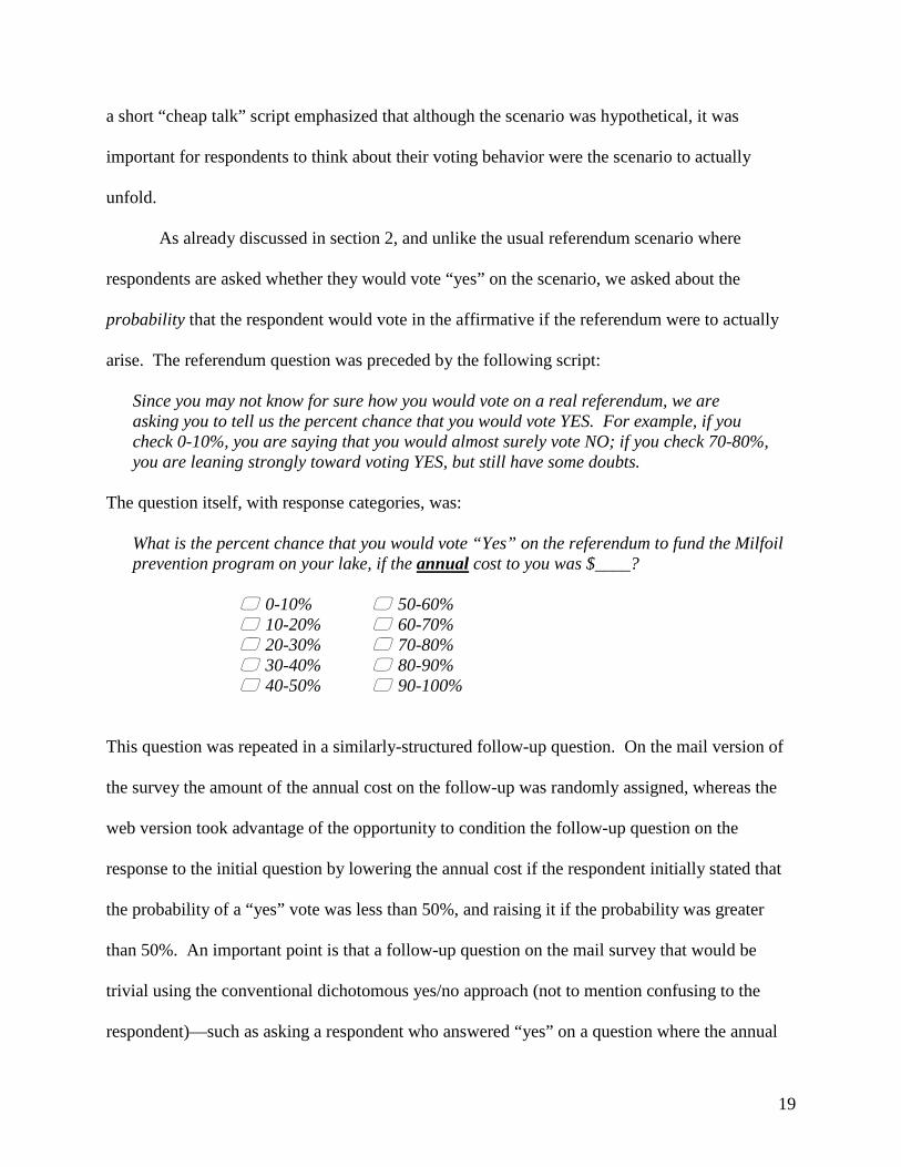
arise. The referendum question was preceded by the following script:

Since you may not know for sure how you would vote on a real referendum, we are asking you to tell us the percent chance that you would vote YES. For example, if you check 0-10%, you are saying that you would almost surely vote NO; if you check 70-80%, you are leaning strongly toward voting YES, but still have some doubts.

The question itself, with response categories, was:

What is the percent chance that you would vote “Yes” on the referendum to fund the Milfoil prevention program on your lake, if the annual cost to you was $____?

0-10% 50-60% 10-20% 60-70% 20-30% 70-80% 30-40% 80-90% 40-50% 90-100%

This question was repeated in a similarly-structured follow-up question. On the mail version of

the survey the amount of the annual cost on the follow-up was randomly assigned, whereas the

web version took advantage of the opportunity to condition the follow-up question on the

response to the initial question by lowering the annual cost if the respondent initially stated that

the probability of a “yes” vote was less than 50%, and raising it if the probability was greater

than 50%. An important point is that a follow-up question on the mail survey that would be

trivial using the conventional dichotomous yes/no approach (not to mention confusing to the

respondent)—such as asking a respondent who answered “yes” on a question where the annual

19

cost is $50 how he would vote if the annual cost were instead $20—provides good information in

the current context because respondents are queried about the probability of their behavior.

Finally, on the Internet survey respondents who indicated on both contingent valuation questions

that their probability of a “yes” vote was 0-10%, or who indicated on both questions that their

probability of a “yes” vote was 90-100%, were asked to state the amount that would leave their

probability of voting “yes” at “about 50%”. Figure 2 presents histograms of respondents’ stated

probability of answering “Yes” to different bid amounts for the Milfoil prevention question. The

striking aspect of figure 2 is how frequently respondents chose a probability category other than

0-10% or 90-100%, indicating substantial respondent uncertainty at all bid levels.

V. Analysis Results

We estimate two models. In the first the systematic portion of the loss function 𝛽𝒛 is

reduced to the constant 𝛽0 (Model 1), and in the second this expression takes the form

𝛽0 + 𝛽1𝐼𝑛𝑐𝑜𝑚𝑒𝑗, where 𝐼𝑛𝑐𝑜𝑚𝑒𝑗 is the annual income of household j (Model 2). We keep

the specifications simple because our focus is on identifying the average household loss Lj

rather than identifying the covariates that condition this loss. Overall, the estimated model

parameters include the constant 𝛽0 /𝜑, the income coefficient 𝛽1 /𝜑, the bid coefficient 1/

𝜑, the discount rate r, the scale ratio 𝜎 /𝜑, and the random effects standard error 𝜗.

Tables 1 and 2 provide estimation results for Models 1 and 2, respectively. The

estimate of mean annual loss from a Milfoil invasion is the sample average value of 𝛽𝒛.10

The mean present value of the loss is the calculated mean annual loss multiplied by 1+𝑟𝑟

.

Average annual willingness to pay to for the prevention program accounts for household

10 Estimation generates 𝛽𝒛𝜑

. Dividing through by the bid coefficient 1𝜑

generates 𝛽𝒛.

20

expectations about the probability of an invasion in the absence of the program, and,

following the modeling of section 2, takes the form,

𝑊𝑇𝑃�������𝑗𝑃𝑃 = 𝑃𝑗(1+𝑟)𝑟+𝑃𝑗

∙ 𝛽𝒛𝑗 . (18)

Confidence intervals are calculated using the Krinsky-Robb (1986) method.

The results support several conclusions. First, all parameters have the expected sign,

and in particular respondents with a higher household income are willing to pay more for a

Milfoil prevention program. Second, the estimated mean welfare loss from a Milfoil

invasion is considerably greater than the estimated mean WTP for the prevention program

because most respondents believe the annual probability of an invasion is fairly low (the

median annual probability is .0315). Third, although the models generate very similar

values for the mean annual WTP for the prevention program (about $570), they generate very

different values for the mean annual loss of an invasion. This is clearly due to differences in

the estimated discount rate (9.7% versus 4.7%), as indicated in equation (6) and confirmed

by a comparison of the present values of the mean welfare loss from the two models, with

Model 2 generating a higher present value even though it generates a lower annual loss.

Section VI. Convergent Validity of the Estimated Welfare Loss

We assessed the convergent validity of the estimated welfare loss from a Milfoil invasion

using two alternative analyses. The first used a contingent valuation question posed to

households with shoreline property on Vilas County lakes already invaded by Milfoil. The

question was presented as a referendum to control the Milfoil invasion to the point where it

would be “highly unlikely” that Milfoil would cause any recreational, aesthetic, or ecological

21

problems on the respondent’s lake.11 The elicitation format was the same as for the Milfoil

prevention question; in particular, we elicited the probability of a “yes” vote on the referendum.

For this question there is no issue of the conflation of expectations and preferences—the welfare

loss from the Milfoil invasion is immediate and certain with probability Pj=1 — and so in

estimation the term 𝑃𝑗(1 + 𝑟)/(𝑟 + 𝑃𝑗) in (12) is eliminated, and otherwise the estimation

proceeds as with the Milfoil prevention case. The sample size is smaller than for the Milfoil

prevention question, because fewer households in the sample reside on lakes already invaded by

Milfoil, with N=233 when household annual income is excluded as a covariate, and N=198 when

it is included.

The second analysis is the recently published hedonic study of Horsch and Lewis (2009).

Using market sales data for shoreline properties in Vilas County, the authors used a difference-

in-differences approach with lake-specific fixed effects to account for the possibility that

unobservables correlated with a lake’s vulnerability to a Milfoil invasion might also affect the

market value of its shoreline properties. The analysis examined over 1800 shoreline property

sales on 172 lakes in Vilas County over the 10-year horizon 1997-2006. Table 3 presents results

of the comparison. Our presumption in the table is that the present value of Milfoil loss is

capitalized in shoreline property values. The Milfoil control analysis did not include estimation

of the discount rate, and so for this analysis we present results for a range of discount rates.

The obvious conclusions to be drawn from this comparison are: i) the cost to shoreline

property owners of a Milfoil invasion are considerable;12 ii) contingent valuation questions do a

11 It is widely understood that once in a lake Milfoil cannot be completely eradicated, and so to present a realistic scenario we chose not to claim it could be. 12 As a point of comparison, average annual income in the sample is $150,000, and the average property value in the Horsch and Lewis (2009) sample was $268,000.

22

reasonable job of estimating the welfare loss from an invasion; and iii) it is possible to separately

identify preferences and expectations in a contingent valuation survey.

On this last point it is instructive to emphasize the consequence of overlooking or

ignoring the issue of respondent expectations of a Milfoil invasion in the absence of a prevention

program, and instead assuming that the estimated WTP for the Milfoil prevention program is a

measure of the welfare loss from an invasion. As presented in the last section, the average value

of the program is $570, far below the welfare loss obtained when expectations are accounted for.

This low value arises because ignoring expectations in the econometric model is structurally

equivalent to removing the term 𝑃𝑗(1+𝑟)𝑟+𝑃𝑗

in (4), so that WTP=L. This, in turn, is equivalent to

setting Pj =1 for all respondents, in which case 𝑃𝑗(1+𝑟)𝑟+𝑃𝑗

= 1 . In other words, in this model

ignoring expectations effectively asserts that all respondents believe that in the absence of the

program an invasion is surely going to occur immediately. Such an overstatement of respondent

expectations naturally leads to an underestimate of the welfare loss.

Section VII. Welfare Estimates from Re-coding Responses

As discussed in the introduction, numerous studies have examined the effect on

welfare estimates of re-coding uncertainty responses as dichotomous Yes/No choices. We

examined this issue using both the data for the Milfoil prevention question, and the data for

the Milfoil control question. In the re-coding, choices below a specified choice probability

category (e.g. 10-20%; see the referendum question above) were re-coded as “No”, and

choices at the probability category and above were re-coded as “Yes”. For the Milfoil

prevention question the model estimated is a logit application of equation (6):

23

Pr(𝑌𝑒𝑠) = Pr�𝑊𝑇𝑃𝑗 > 𝑡𝑗� = 𝑃𝑟 �𝑃𝑗(1+𝑟)

𝑟+𝑃𝑗∙ 𝐿�𝒛𝑗� − 𝑡𝑗 > 𝜀𝑗� =

𝑒𝑥𝑝�𝑃𝑗(1+𝑟)

𝑟+𝑃𝑗∙𝐿�𝒛𝒋�𝜎 −

𝑡𝑗𝜎�

1+𝑒𝑥𝑝�𝑃𝑗(1+𝑟)

𝑟+𝑃𝑗∙𝐿�𝒛𝒋�𝜎 −

𝑡𝑗𝜎�

,

where the discount rate r is fixed at its value estimated in Model 1 (r=0.02), and the loss

function takes the form used in Model 1, 0( )jL β=z . For the Milfoil control question, the

logit form is the same as this, but with the term 𝑃𝑗(1+𝑟)

𝑟+𝑃𝑗 omitted, because, as indicated in the

previous section, there is no conflation of expectations and preferences concerning the

presence of Milfoil. Because income was not included as an explanatory variable, sample

sizes were 900 and 233 for the prevention and control models, respectively.

This model was estimated for all nine feasible re-coding possibilities. In other words,

the model was estimated by using as probability boundaries for the No/Yes re-coding the

levels 10%, 20%, 30%...90%. For example, for the model where the probability boundary

was 10%, the probability choice category “0-10% was coded “No”, and the choice categories

“10-20%” and higher were coded “Yes”.

Figure 3 presents the results of this analysis. As expected, as the probability

boundary increases, the estimated average welfare gain from prevention/control decreases.

The average welfare gain for the model where respondent uncertainty is accounted for is

$2106 for Milfoil prevention and $1226 for Milfoil control (the values in Table 1 when

income is excluded as a variable). The recoding boundaries generating the closest values to

these are 60% for both Milfoil prevention (welfare gain equals $2237) and Milfoil control

($1082).

24

Section VIII. Conclusion

Concerning the use of surveys to measure expectations, Manski (2004. pg. 42) concluded,

“Economists have long been hostile to subjective data. Caution is prudent, but hostility is not warranted…We have learned enough for me to recommend, with some confidence, that economists should abandon their antipathy to measurement of expectations. The unattractive alternative to measurement is to make unsubstantiated assumptions”.

This analysis extends this perspective to identifying the value of an environmental good in

contingent valuation. To minimize complications from so-called “hypothetical bias”, contingent

valuation often involves the presentation of a valuation scenario in which the respondent is asked

to pay or donate to a program of environmental improvement. The WTP calculated from this

scenario is often a conflation of preferences over the environmental improvement and

expectations concerning the state of the environmental good in the absence of the program. To

the extent that interest lies primarily in the welfare gain from the environmental improvement per

se, it is incumbent to separate preferences and expectations; in other words, to understand the

welfare gain associated with an environmental good, or the welfare loss associated with an

environmental bad, it is critical to understand the respondent’s judgment about the outcomes in

the absence of the program. One way to do this involves surveying households about their

expectations, and our analysis provides theoretical and methodological particulars for the case

where the environmental improvement is binary.

We are cautiously optimistic about the potential for survey questions to parse

expectations and preferences, albeit with the following caveats/recommendations. First, in

hindsight we believe that for binary environmental events such as exotic species invasions it

would be well worth the effort and questionnaire space to ask respondents more than one

question about the probability of the event in the absence of a change in management or policy.

25

This allows relaxing the assumption that respondents believe the annual probability of the

environmental event is constant. For instance, respondents could be queried about the

probability of the event over 5-year and 10-year horizons.

A second and related point is that if the environmental improvement is not binary then

the issue of identifying expectations becomes more complex because the issue is no longer when

an event occurs, but the evolution of the environmental change. Consider, for instance, that it is

easier to estimate a reasonable model of respondent expectations about the binary state of

development of a particular shoreline parcel over a 10-year horizon than it is to estimate a model

of expectations about the rate of development of the entire shoreline.

Finally, we suspect that the greater the respondent’s familiarity with the environmental

good in question, the more likely it is that the respondent can articulate expectations about future

changes in the good, and the more important it is to allow respondents to express their subjective

expectations about future changes in the good. For a mail survey, focus groups, pilot studies,

and the analyst’s intuitive sense should guide the decision about whether to elicit respondent

expectations. In our view the most sensible way to proceed on telephone and web surveys is to

probe whether the respondent has expectations about future changes in the good, and to direct

respondents with strong expectations to a series of questions to measure these expectations, and

to direct other respondents to a series of statements to form their expectations. A valuable

research agenda would be to examine differences in the variation in WTP between respondents

with strong and weak (or no clear) expectations. We hypothesize lower variation in WTP for

respondents with strong expectations (controlling for covariates), because such respondents have

spent more time thinking about the good.

26

27

References

Adamowicz, W., Swait, J., Boxall, P., Louviere, J., Williams, M. 1997. “Perceptions versus objective measures of environmental quality in combined Revealed and Stated Preference models of environmental valuation”. Journal of Environmental Economics and Management 32 (1), 65-84. Alberini, A., K. Boyle, and M. Welsh. 2003. “Analysis of Contingent Valuation Data with Multiple Bids and Response Options Allowing Respondents to Express Uncertainty.” Journal of Environmental Economics and Management 45: 40-62. Berrens, R.P., H. Jenkins-Smith, A. K. B., and C.L. Silva. 2002. “Further Investigation of Voluntary Contribution Contingent Valuation: Fair Share, Time of Contribution, and Respondent Uncertainty.” Journal of Environmental Economics and Management 44: 144-168. Blomquist, G.C., K. Blumenschein, and M. Johannesson. 2009. “Eliciting willingness to pay without bias using follow-up certainty statements: Comparisons between probably/definitely and a 10-point certainty scale.” Environmental and Resource Economics 43: 473-502. Blomquist, G.C., and J.C. Whitehead. 1998. “Resource quality information and validity of willingness to pay in contingent valuation”. Resource and Energy Economics 20: 179–196. Blumenschein, K., K. Johannesson, G.C. Blomquist, R. Liljas, and R.M. O’Conor. 1998. “Experimental results on expressed certainty and hypothetical bias in contingent valuation.” Southern Economic Journal 65(1): 169-177. Boyle, Kevin J. 2003. “Contingent Valuation in Practice”. In: A Primer on Nonmarket Valuation (Patricia A. Champ, Kevin J. Boyle, and Thomas C. Brown, eds.), Kluwer Academic Publishers, Norwell, MA. Burghart, D.R., T.A. Cameron, and G.R. Gerdes. 2007. “Valuing publicly sponsored research projects: risks, scenario adjustments, and inattention.” Journal of Risk and Uncertainty 35: 77-105. Champ, P.A., R.C. Bishop, T.C. Brown, and D.W. McCollum. 1997. “Using donation mechanisms to value nonuse benefits from public goods.” Journal of Environmental Economics and Management 33(2): 151-162. Champ, P.A. and R.C. Bishop. 2001. “Donation payment mechanisms and contingent valuation: an empirical study of hypothetical bias.” Environmental Resource Economics 19: 383-402. Champ, P.A., R.C. Bishop, and R. Moore. 2002. “Approaches to mitigating hypothetical bias.” Proceedings from 2005 Western Regional Research Project W-1133: Benefits and Costs in Natural Resource Planning, Salt Lake City, UT.

28

Delavande, A., X. Giné, and D. McKenzie. 2011. “Measuring subjective expectations in developing countries: A critical review and new evidence”. Journal of Development Economics 94(2): 151-163. DeShazo, J.R. and T.A. Cameron. 2005. “The effect of health status on willingness to pay for morbidity and mortality risk reductions.” California Center for Population Research, On-Line Working Paper Series CCPR-050-05. http://escholarship.org/uc/item/9431841p. Evans, M.F., N.E. Flores, and K.J. Boyle. 2003. “Multiple-bounded uncertainty choice data as probabilistic intentions.” Land Economics 79: 549-560. Hoehn, J.P. and A. Randall. 2002. “The effect of resource quality information on resource injury perceptions and contingent values”. Resource and Energy Economics 24: 13-31. Horsch, E.J. and D.J. Lewis. 2009. “The effects of aquatic invasive species on property values: evidence from a quasi-experiment.” Land Economics 85(3):391-409. Hurd, M.D. 2009. “Subjective probabilities in household surveys.” Annual Review of Economics 1:543-562. Kataria, M., I. BatemanT. Christensen, A. Dubgaard, B. Hasler, S. Hime, J. Ladenburg, G. Levin, L. Martinsen, and C. Nissen. 2012. “Scenario realism and welfare estimates in choice experiments –a nonmarket valuation study on the European water framework directive”. Journal of Environmental Management 94(1): 25-33. Kovacs, K.F. and D.M. Larson. 2008. “Identifying individual discount rates and valuing public open space with stated-preference models.” Land Economics 84(2):209-224. Krinsky, I., and A. Robb. 1986. “On approximating the statistical properties of elasticities.” The Review of Economics and Statistics 86, 715–719. Li, C. Z., and L. Mattsson. 1995. “Discrete Choice Under Preference Uncertainty: An Improved Structural Model for Contingent Valuation.” Journal of Environmental Economics and Management 28: 256-269. Manski, Charles F. 2004. “Measuring expectations.” Econometrica 72(5): 1329-1376. Moore, R., R.C. Bishop, B. Provencher, and P.A. Champ. 2010. “Accounting for Respondent Uncertainty to Improve Willingness-to-Pay Estimates”. Canadian Journal of Agricultural Economics 58(3): 381-401. Ready, R., J. Whitehead, and G. Blomquist. 1995. “Contingent valuation when respondents are ambivalent”. J. Environ. Econom. Management 29: 181–196. Rubin, J., G. Helfand, and J. Loomis. 1991. “A benefit-cost analysis of the Northern Spotted Owl.” Journal of Forestry 89(12): 25-30.

29

Samnaliev, M., T.H. Stevens, and T. More. 2006. “A comparison of alternative certainty calibration techniques in contingent valuation.” Ecological Economics 57: 507-519. Smith, C. S., and J. W. Barko. 1990. “Ecology of eurasian watermilfoil.’’ Journal of Aquatic Plant Management 28 (2): 55–64. Stumborg, B.E., K.A. Baerenklau, and R.C. Bishop. 2001. “Nonpoint source pollution and present values: a contingent valuation study of Lake Mendota.” Review of Agricultural Economics 23(1):120-132. Tkac, Jennifer, 1998. “ The effects of information on willingness-to-pay values of endangered species”. American Journal of Agricultural Economics 80: 1214–1220. Vander Zanden, M. J., K. A. Wilson, J. M.Casselman, and N. D. Yan. 2004. ‘‘Species Introductions and Their Impacts in North American Shield Lakes.’’ In Boreal Shield Watersheds: Lake Trout Ecosystems in a Changing Environment, ed. J. M. Gunn, R. A. Ryder, and R. J. Steedman. Boca Raton, FL: CRC Press. Wang, H. and D. Whittington. 2005. "Measuring individuals' valuation distributions using a stochastic payment card approach." Ecological Economics, 55 143-154. Welsh, M.P., and G.L. Poe. 1998. “Elicitation Effects in Contingent Valuation: Comparisons to a Multiple Bounded Discrete Choice Approach.” Journal of Environmental Economics and Management 36: 170-185.

30

Figure 1. Histogram of Respondent Expectations of Future Milfoil Invasion

0

0.05

0.1

0.15

0.2

0.25

Stated Probability of Milfoil Invasion in Next Ten Years

Perc

ent

31

Figure 2. Histograms of Respondents’ Stated Probability of Answering “Yes” to a Bid Amount for the Milfoil prevention question.

2.1 Bid Amounts less than $100 2.2 Bid Amounts between $100 and $250

2.3 Bid Amounts between $251 and $500 2.4 Bid Amounts greater than $500

00.05

0.10.15

0.20.25

0.30.35

0.4

Stated Probability of Answering "Yes" to Bid Amount

Perc

ent C

hose

n

00.05

0.10.15

0.20.25

0.30.35

0.4

Stated Probability of Answering "Yes" to Bid Amount Pe

rcen

t Cho

sen

00.05

0.10.15

0.20.25

0.30.35

0.4

Stated Probability of Answering "Yes" to Bid Amount

Perc

ent C

hose

n

00.05

0.10.15

0.20.25

0.30.35

0.4

Stated Probability of Answering "Yes" to Bid Amount

Perc

ent C

hose

n

32

Figure 3. Estimate of Average Welfare Gain from Milfoil Prevention/Control as a Function of the Probability Threshold at Which Responses are Coded Yes vs. No.

-6000

-4000

-2000

0

2000

4000

6000

8000

10000

0% 10% 20% 30% 40% 50% 60% 70% 80% 90% 100%

Milfoil Prevention Milfoil Control

Threshold

Wel

fare

Gai

n ($

)

33

Table 1. Estimation Results for Model 1 (Household income not included; N=900)

Parameter Estimate Standard Error

t-Statistic

Discount Rate (r) 0.098 0.048 2.022 Bid coefficient (1/𝜑) 0.793 0.116 6.807 Scale ratio (𝜎/𝜑) 0.669 0.021 31.725 Constant (𝛽0/𝜑) 1.670 0.409 4.079 Random effects standard deviation (𝜗) 1.782 0.385 4.628

Mean 95% Confidence Interval Sample mean estimated annual loss from a Milfoil invasion ($)

2,106 {1312, 3492}

Sample mean estimated present value of loss from a Milfoil invasion ($)

23,614 {14,709, 39,145}

Sample mean estimated annual WTP for the prevention program ($)

563 {351, 933}

34

Table 2. Estimation Results for Model 2 (Household income included; N=762)

Parameter Estimate Standard Error

t-Statistic

Discount Rate (r) 0.047 0.029 1.621 Bid coefficient (1/𝜑) 1.057 0.166 6.385 Scale ratio (𝜎/𝜑) 0.704 0.029 23.967 Constant (𝛽0/𝜑) 0.881 0.280 3.141 Income coefficient (𝛽1/𝜑) 3.828 0.932 4.105 Random effects standard deviation (𝜗) 1.520 0.264 5.751 Mean 95% Confidence Interval Sample mean estimated annual loss from a Milfoil invasion ($) 1,373 {777, 2153}

Sample mean estimated present value of loss from a Milfoil invasion ($) 30,550 {17,283, 47,884}

Sample mean estimated annual WTP for the prevention program ($) 577 {326, 904}

35

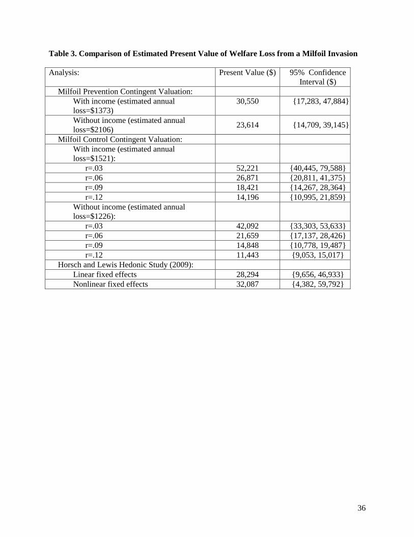
Table 3. Comparison of Estimated Present Value of Welfare Loss from a Milfoil Invasion

Analysis: Present Value ($) 95% Confidence Interval ($)

Milfoil Prevention Contingent Valuation: With income (estimated annual loss=$1373)

30,550 {17,283, 47,884}

Without income (estimated annual loss=$2106) 23,614 {14,709, 39,145}

Milfoil Control Contingent Valuation: With income (estimated annual

loss=$1521):

r=.03 52,221 {40,445, 79,588} r=.06 26,871 {20,811, 41,375} r=.09 18,421 {14,267, 28,364} r=.12 14,196 {10,995, 21,859} Without income (estimated annual

loss=$1226):

r=.03 42,092 {33,303, 53,633} r=.06 21,659 {17,137, 28,426} r=.09 14,848 {10,778, 19,487} r=.12 11,443 {9,053, 15,017} Horsch and Lewis Hedonic Study (2009): Linear fixed effects 28,294 {9,656, 46,933} Nonlinear fixed effects 32,087 {4,382, 59,792}

36

Appendix 1. Derivation of equation (11)

The observed probability of accepting the bid payment tj has a lower bound 𝜋𝑗𝐿 and an upper

bound 𝜋𝑗𝐻 . Formally, we have,

𝜋𝑗𝐿 <𝑒𝑥𝑝�

𝑃𝑗(1+𝑟)𝑟+𝑃𝑗

∙𝛽𝑧𝑗+𝑣𝑗

𝜎 − 𝑡𝑗𝜎�

1+𝑒𝑥𝑝�𝑃𝑗(1+𝑟)𝑟+𝑃𝑗

∙𝛽𝑧𝑗+𝑣𝑗

𝜎 − 𝑡𝑗𝜎�

< 𝜋𝑗𝐻 (A1)

It follows that the probability of the respondent choosing probability category Cj, conditional on

parameters 𝛽, is the probability that 𝑣𝑗 lies between values {𝑎, 𝑏} :

Pr�𝐶𝑗� = Pr (a < 𝑣𝑗 < 𝑏|𝛽) . (A2)

Multiply both sides of (A1) by 1 + 𝑒𝑥𝑝 �𝑃𝑗(1+𝑟)𝑟+𝑃𝑗

∙ 𝛽𝑧𝑗+𝑣𝑗𝜎

− 𝑡𝑗𝜎�:

[1 + 𝑒𝑥𝑝 �𝑃𝑗(1+𝑟)𝑟+𝑃𝑗

∙ 𝛽𝑧𝑗+𝑣𝑗𝜎

− 𝑡𝑗𝜎�]𝜋𝑗𝐿 < 𝑒𝑥𝑝 �𝑃𝑗(1+𝑟)

𝑟+𝑃𝑗∙ 𝛽𝑧𝑗+𝑣𝑗

𝜎 − 𝑡𝑗

𝜎� < [1 + 𝑒𝑥𝑝 �𝑃𝑗(1+𝑟)

𝑟+𝑃𝑗∙

𝛽𝑧𝑗+𝑣𝑗𝜎

− 𝑡𝑗𝜎�]𝜋𝑗𝐻 (A3)

Now, multiply (A3) through by 𝑒𝑥𝑝 �𝑡𝑗𝜎− 𝑃𝑗(1+𝑟)

𝑟+𝑃𝑗∙ 𝛽𝑧𝑗𝜎

�:

�𝑒𝑥𝑝 �𝑡𝑗𝜎− 𝑃𝑗(1+𝑟)

𝑟+𝑃𝑗∙ 𝛽𝑧𝑗𝜎

� + 𝑒𝑥𝑝 �𝑣𝑗𝜎�� 𝜋𝑗𝐿 < 𝑒𝑥𝑝 � 𝑣𝑗

𝜎� < [𝑒𝑥𝑝 �𝑡𝑗

𝜎− 𝑃𝑗(1+𝑟)

𝑟+𝑃𝑗∙ 𝛽𝑧𝑗𝜎� + 𝑒𝑥𝑝 �𝑣𝑗

𝜎�]𝜋𝑗𝐻. (A4)

Therefore,

𝜋𝑗𝐿𝑒𝑥𝑝 �𝑡𝑗𝜎− 𝑃𝑗(1+𝑟)

𝑟+𝑃𝑗∙ 𝛽𝑧𝑗𝜎

� < �1 − 𝜋𝑗𝐿�𝑒𝑥𝑝 � 𝑣𝑗𝜎� and

�1 − 𝜋𝑗𝐻�𝑒𝑥𝑝 � 𝑣𝑗𝜎� < 𝜋𝑗𝐻𝑒𝑥𝑝 �

𝑡𝑗𝜎− 𝑃𝑗(1+𝑟)

𝑟+𝑃𝑗∙ 𝛽𝑧𝑗𝜎

� .

Therefore,

𝜋𝑗𝐿(1−𝜋𝑗𝐿)

𝑒𝑥𝑝 �𝑡𝑗𝜎− 𝑃𝑗(1+𝑟)

𝑟+𝑃𝑗∙ 𝛽𝑧𝑗𝜎

� < 𝑒𝑥𝑝 � 𝑣𝑗𝜎� < 𝜋𝑗𝐻

(1−𝜋𝑗𝐻) 𝑒𝑥𝑝 �𝑡𝑗

𝜎− 𝑃𝑗(1+𝑟)

𝑟+𝑃𝑗∙ 𝛽𝑧𝑗𝜎

� . (A5)

Taking logs of both sides of (A5),

37

σln � 𝜋𝑗𝐿(1−𝜋𝑗𝐿)

𝑒𝑥𝑝 �𝑡𝑗𝜎− 𝑃𝑗(1+𝑟)

𝑟+𝑃𝑗∙ 𝛽𝑧𝑗𝜎

�� < 𝑣𝑗 < σln � 𝜋𝑗𝐻(1−𝜋𝑗𝐻)

𝑒𝑥𝑝 �𝑡𝑗𝜎− 𝑃𝑗(1+𝑟)

𝑟+𝑃𝑗∙ 𝛽𝑧𝑗𝜎

��.

Therefore,

𝑡𝑗 −𝑃𝑗(1+𝑟)𝑟+𝑃𝑗

∙ 𝛽𝑧𝑗 + σln � 𝜋𝑗𝐿(1−𝜋𝑗𝐿)

� < 𝑣𝑗 < 𝑡𝑗 −𝑃𝑗(1+𝑟)𝑟+𝑃𝑗

∙ 𝛽𝑧𝑗 + σln � 𝜋𝑗𝐻(1−𝜋𝑗𝐻)

� . (A6)

Equation (A6) is equation (11) in the text.

Appendix 2. Derivation of equation (12)

Considering equation (11), which identifies bounds on 𝑣𝑗 , the probability of the observed

category 𝐶𝑗 is:

𝑃𝑟 �𝑡 − 𝑃𝑗(1+𝑟)𝑟+𝑃𝑗

𝛽𝒛𝑗 + 𝜎𝑙𝑛 � 𝜋𝑗𝐿(1−𝜋𝑗𝐿)

� < 𝑣𝑗 < 𝑡 − 𝑃𝑗(1+𝑟)𝑟+𝑃𝑗

∙ 𝛽𝒛𝑗 + 𝜎𝑙𝑛 � 𝜋𝑗𝐻(1−𝜋𝑗𝐻)

��

If 𝑣𝑗 has a logistic distribution with mean 𝜇 and scale parameter 𝜑, then,

𝑃𝑟 �𝑣𝑗 < 𝑡 − 𝑃𝑗(1+𝑟)𝑟+𝑃𝑗

∙ 𝛽𝒛𝑗 + 𝜎𝑙𝑛 � 𝜋𝑗(1−𝜋𝑗)

�� = 1

1+𝑒𝑥𝑝�𝜇−�𝑡−

𝑃𝑗(1+𝑟)𝑟+𝑃𝑗

∙𝛽𝒛𝑗+𝜎𝑙𝑛�𝜋𝑗

(1−𝜋𝑗)��

𝜑 �

=1

1 + exp �𝜇𝜑� 𝑒𝑥𝑝 �𝑡 −𝑃𝑗(1 + 𝑟)𝑟 + 𝑃𝑗

∙ 𝛽𝒛𝑗 + 𝜎𝑙𝑛 �𝜋𝑗

(1 − 𝜋𝑗)��−1𝜑

=1

1 + exp �𝜇 +

𝑃𝑗(1 + 𝑟)𝑟 + 𝑃𝑗

∙ 𝛽𝒛𝑗 − 𝑡

𝜑 � �1 − 𝜋𝑗𝜋𝑗

�𝜎/𝜑

Therefore, since 𝜇=0 when the vector 𝒛𝑗 includes a constant, the probability of the observed

response is,

Pr�𝐶𝑗� = 1

1+exp �

𝑃𝑗(1+𝑟)𝑟+𝑃𝑗

∙𝛽𝒛𝑗−𝑡

𝜑 ∙�∙�(1−𝜋𝑗𝐻)𝜋𝑗𝐻

�σ/φ− 1

1+exp �

𝑃𝑗(1+𝑟)𝑟+𝑃𝑗

∙𝛽𝒛𝑗−𝑡

𝜑 ∙�∙�(1−𝜋𝑗𝐿)𝜋𝑗𝐿

�σ/φ

(A7)

38