Disk-Covering Methods for phylogeny reconstruction

Tandy Warnow

The University of Texas at Austin

Phylogeny

Orangutan Gorilla Chimpanzee Human

From the Tree of the Life Website,University of Arizona

Reconstructing the “Tree” of Life

Handling large datasets: Handling large datasets: millions of speciesmillions of species

NSF funds many projectsNSF funds many projectstowards this goal, undertowards this goal, underthethe Assembling the Tree of Assembling the Tree of Life (ATOL) Life (ATOL) programprogram

DNA Sequence Evolution

AAGACTT

TGGACTTAAGGCCT

-3 mil yrs

-2 mil yrs

-1 mil yrs

today

AGGGCAT TAGCCCT AGCACTT

AAGGCCT TGGACTT

TAGCCCA TAGACTT AGCGCTTAGCACAAAGGGCAT

AGGGCAT TAGCCCT AGCACTT

AAGACTT

TGGACTTAAGGCCT

AGGGCAT TAGCCCT AGCACTT

AAGGCCT TGGACTT

AGCGCTTAGCACAATAGACTTTAGCCCAAGGGCAT

Phylogeny Problem

TAGCCCA TAGACTT TGCACAA TGCGCTTAGGGCAT

U V W X Y

U

V W

X

Y

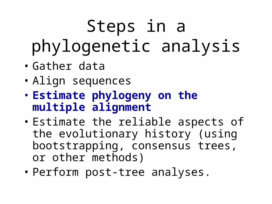
Steps in a phylogenetic analysis

• Gather data• Align sequences• Estimate phylogeny on the multiple

alignment • Estimate the reliable aspects of the

evolutionary history (using bootstrapping, consensus trees, or other methods)

• Perform post-tree analyses.

1. Hill-climbing heuristics for hard optimization criteria (Maximum Parsimony and Maximum Likelihood)

Phylogenetic reconstruction methods

Phylogenetic trees

Cost

Global optimum

Local optimum

2. Polynomial time distance-based methods: Neighbor Joining, FastME, Weighbor, etc.

3. Bayesian methods

Performance criteria

• Running time.• Space.• Statistical performance issues (e.g., statistical

consistency) with respect to a Markov model of evolution.

• “Topological accuracy” with respect to the underlying true tree. Typically studied in simulation.

• Accuracy with respect to a particular criterion (e.g. tree length or likelihood score), on real data.

Markov models of site evolution

Simplest (Jukes-Cantor):• The model tree is a pair (T,{e,p(e)}), where T is a rooted binary

tree, and p(e) is the probability of a substitution on the edge e• The state at the root is random• If a site changes on an edge, it changes with equal probability to

each of the remaining states• The evolutionary process is MarkovianMore complex models (such as the General Markov model) are

also considered, with little change to the theory. Variation between different sites is either prohibited or minimized,

in order to ensure identifiability of the model.

Distance-based Phylogenetic Methods

Maximum Parsimony

• Input: Set S of n aligned sequences of length k• Output:

– A phylogenetic tree T leaf-labeled by sequences in S

– additional sequences of length k labeling the internal nodes of T

such that is minimized, where H(i,j) denotes the Hamming distance between sequences at nodes i and j

∑∈ )(),(

),(TEji

jiH

Maximum Likelihood

• Input: Set S of n aligned sequences of length k, and a specified parametric model

• Output: – A phylogenetic tree T leaf-labeled by sequences in S– With additional model parameters (e.g. edge “lengths”)

such that Pr[S|(T, params)] is maximized.

1. Hill-climbing heuristics (which can get stuck in local optima)2. Randomized algorithms for getting out of local optima3. Approximation algorithms for MP (based upon Steiner Tree

approximation algorithms).

Approaches for “solving” MP/ML

Phylogenetic trees

Cost

Global optimum

Local optimum

Theoretical results

• Neighbor Joining is polynomial time, and statistically consistent under typical models of evolution.

• Maximum Parsimony is NP-hard, and even exact solutions are not statistically consistent under typical models.

• Maximum Likelihood is NP-hard and statistically consistent under typical models.

Theoretical convergence rates

• Atteson: Let T be a General Markov model tree defining additive matrix D. Then Neighbor Joining will reconstruct the true tree with high probability from sequences that are of length at least O(lg n emax Dij).

• Proof: Show NJ accurate on input matrix d such that max{|Dij-dij|}<f/2, for f equal to the minimum edge “length”.

Problems with NJ

• Theory: The convergence rate is exponential: the number of sites needed to obtain an accurate reconstruction of the tree with high probability grows exponentially in the evolutionary diameter.

• Empirical: NJ has poor performance on datasets with some large leaf-to-leaf distances.

Quantifying Error

FN: false negative (missing edge)FP: false positive (incorrect edge)

50% error rate

FN

FP

Neighbor joining has poor performance on large diameter trees [Nakhleh et al. ISMB 2001]

Simulation study based upon fixed edge lengths, K2P model of evolution, sequence lengths fixed to 1000 nucleotides.

Error rates reflect proportion of incorrect edges in inferred trees.

NJ

0 400 800 16001200No. Taxa

0

0.2

0.4

0.6

0.8

Err

or R

ate

• Other standard polynomial time methods don’t improve substantially on NJ (and have the same problem with large diameter datasets).

• What about trying to “solve” maximum parsimony or maximum likelihood?

Solving NP-hard problems exactly is … unlikely

• Number of (unrooted) binary trees on n leaves is (2n-5)!!

• If each tree on 1000 taxa could be analyzed in 0.001 seconds, we would find the best tree in

2890 millennia

#leaves #trees

4 3

5 15

6 105

7 945

8 10395

9 135135

10 2027025

20 2.2 x 1020

100 4.5 x 10190

1000 2.7 x 102900

How good an MP analysis do we need?

• Our research shows that we need to get within 0.01% of optimal (or better even, on large datasets) to return reasonable estimates of the true tree’s “topology”

Problems with current techniques for MP

0

0.02

0.04

0.06

0.08

0.1

0.12

0.14

0.16

0.18

0.2

0 4 8 12 16 20 24

Hours

Average MP score above

optimal, shown as a percentage of

the optimal

Shown here is the performance of a heuristic maximum parsimony analysis on a real dataset of almost 14,000 sequences. (“Optimal” here means best score to date, using any method for any amount of time.) Acceptable error is below 0.01%.

Performance of TNT with time

Empirical problems with existing methods

• Heuristics for Maximum Parsimony (MP) and Maximum Likelihood (ML) cannot handle large datasets (take too long!) – we need new heuristics for MP/ML that can analyze large datasets

• Polynomial time methods have poor topological accuracy on large diameter datasets – we need better polynomial time methods

Using divide-and-conquer

• Conjecture: better (more accurate) solutions will be found if we analyze a small number of smaller subsets and then combine solutions

• Note: different “base” methods will need potentially different decompositions.

• Alert: the subtree compatibility problem is NP-complete!

Using divide-and-conquer

• Conjecture: better (more accurate) solutions will be found if we analyze a small number of smaller subsets and then combine solutions

• Note: different “base” methods will need potentially different decompositions.

• Alert: the subtree compatibility problem is NP-complete!

Using divide-and-conquer

• Conjecture: better (more accurate) solutions will be found if we analyze a small number of smaller subsets and then combine solutions

• Note: different “base” methods will need potentially different decompositions.

• Alert: the subtree compatibility problem is NP-complete!

DCMs: Divide-and-conquer for improving phylogeny reconstruction

Strict Consensus Merger (SCM)

“Boosting” phylogeny reconstruction methods

• DCMs “boost” the performance of phylogeny reconstruction methods.

DCMBase method M DCM-M

DCMs (Disk-Covering Methods)

• DCMs for polynomial time methods improve topological accuracy (empirical observation), and have provable theoretical guarantees under Markov models of evolution

• DCMs for hard optimization problems reduce running time needed to achieve good levels of accuracy (empirically observation)

Absolute fast convergence vs. exponential convergence

DCM-Boosting [Warnow et al. 2001]

• DCM+SQS is a two-phase procedure which reduces the sequence length requirement of methods.

DCM SQSExponentiallyconvergingmethod

Absolute fast convergingmethod

DCM1 Decompositions

DCM1 decomposition : compute the maximal cliques

Input: Set S of sequences, distance matrix d, threshold value

1. Compute threshold graph }),(:),{(,),,( qjidjiESVEVGq ≤===

2. Perform minimum weight triangulation

}{ ijdq∈

DCM1-boosting distance-based methods[Nakhleh et al. ISMB 2001]

•DCM1-boosting makes distance-based methods more accurate

•Theoretical guarantees that DCM1-NJ converges to the true tree from polynomial length sequences

NJ

DCM1-NJ

0 400 800 16001200No. Taxa

0

0.2

0.4

0.6

0.8

Err

or R

ate

Major challenge: MP and ML

• Maximum Parsimony (MP) and Maximum Likelihood (ML) remain the methods of choice for most systematists

• The main challenge here is to make it possible to obtain good solutions to MP or ML in reasonable time periods on large datasets

Maximum Parsimony

• Input: Set S of n aligned sequences of length k

• Output: A phylogenetic tree T– leaf-labeled by sequences in S– additional sequences of length k labeling the

internal nodes of T

such that is minimized. ∑∈ )(),(

),(TEji

jiH

Maximum parsimony (example)

• Input: Four sequences– ACT– ACA– GTT– GTA

• Question: which of the three trees has the best MP scores?

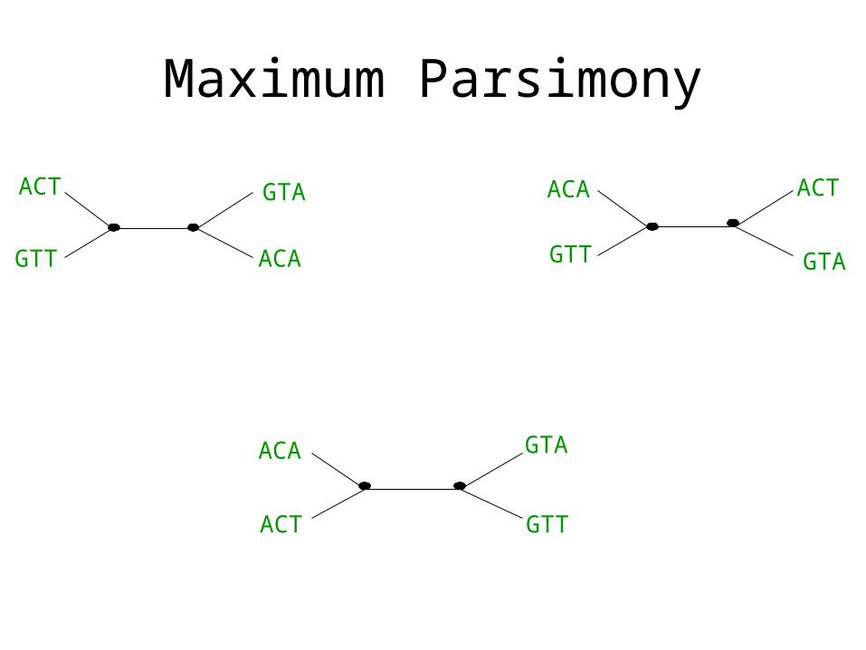
Maximum Parsimony

ACT

GTT ACA

GTA ACA ACT

GTAGTT

ACT

ACA

GTT

GTA

Maximum Parsimony

ACT

GTT

GTT GTA

ACA

GTA

12

2

MP score = 5

ACA ACT

GTAGTT

ACA ACT

3 1 3

MP score = 7

ACT

ACA

GTT

GTAACA GTA

1 2 1

MP score = 4

Optimal MP tree

Maximum Parsimony: computational complexity

ACT

ACA

GTT

GTAACA GTA

1 2 1

MP score = 4

Finding the optimal MP tree is NP-hard

Optimal labeling can becomputed in linear time O(nk)

Problems with current techniques for MP

0

0.02

0.04

0.06

0.08

0.1

0.12

0.14

0.16

0.18

0.2

0 4 8 12 16 20 24

Hours

Average MP score above

optimal, shown as a percentage of

the optimal

Best methods are a combination of simulated annealing, divide-and-conquer and genetic algorithms, as implemented in the software package TNT. However, theydo not reach 0.01% of optimal on large datasets in 24 hours.

Performance of TNT with time

Observations

• The best MP heuristics cannot get acceptably good solutions within 24 hours on most of these large datasets.

• Datasets of these sizes may need months (or years) of further analysis to reach reasonable solutions.

• Apparent convergence can be misleading.

Our objective: speed up the best MP heuristics

Time

MP scoreof best trees

Performance of hill-climbing heuristic

Desired Performance

Fake study

Divide-and-conquer technique for speeding up MP/ML searches

DCM Decompositions

DCM1 decomposition : DCM2 decomposition: Clique-separator plus component

Input: Set S of sequences, distance matrix d, threshold value

1. Compute threshold graph }),(:),{(,),,( qjidjiESVEVGq ≤===

2. Perform minimum weight triangulation

}{ ijdq∈

Empirical observation

• DCM1 not as good as DCM2 for MP

• DCM2 decompositions too large, too slow to compute.

• Neither improved the best MP heuristics.

How can we improve upon existing techniques?

Tree Bisection and Reconnection (TBR)

Tree Bisection and Reconnection (TBR)

Delete an edge

Tree Bisection and Reconnection (TBR)

Tree Bisection and Reconnection (TBR)

Reconnect the trees with a new edgethat bifurcates an edge in each tree

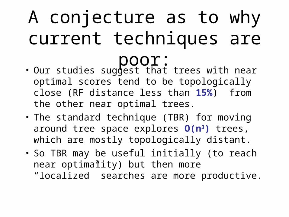
A conjecture as to why current techniques are poor:

• Our studies suggest that trees with near optimal scores tend to be topologically close (RF distance less than 15%) from the other near optimal trees.

• The standard technique (TBR) for moving around tree space explores O(n3) trees, which are mostly topologically distant.

• So TBR may be useful initially (to reach near optimality) but then more “localized” searches are more productive.

Using DCMs differently

• Observation: DCMs make small local changes to the tree

• New algorithmic strategy: use DCMs iteratively and/or recursively to improve heuristics on large datasets

• However, the initial DCMs for MP – produced large subproblems and – took too long to compute

• We needed a decomposition strategy that produces small subproblems quickly.

Using DCMs differently

• Observation: DCMs make small local changes to the tree

• New algorithmic strategy: use DCMs iteratively and/or recursively to improve heuristics on large datasets

• However, the initial DCMs for MP – produced large subproblems and – took too long to compute

• We needed a decomposition strategy that produces small subproblems quickly.

Using DCMs differently

• Observation: DCMs make small local changes to the tree

• New algorithmic strategy: use DCMs iteratively and/or recursively to improve heuristics on large datasets

• However, the initial DCMs for MP – produced large subproblems and – took too long to compute

• We needed a decomposition strategy that produces small subproblems quickly.

New DCM3 decomposition

Input: Set S of sequences, and guide-tree T

1. Compute short subtree graph G(S,T), based upon T

2. Find clique separator in the graph G(S,T) and form subproblems

DCM3 decompositions (1) can be obtained in O(n) time(2) yield small subproblems(3) can be used iteratively

Iterative-DCM3

T

T’

Base methodDCM3

New DCMs

• DCM31. Compute subproblems using DCM3 decomposition

2. Apply base method to each subproblem to yield subtrees

3. Merge subtrees using the Strict Consensus Merger technique

4. Randomly refine to make it binary

• Recursive-DCM3• Iterative DCM3

1. Compute a DCM3 tree

2. Perform local search and go to step 1

• Recursive-Iterative DCM3

Datasets

• 1322 lsu rRNA of all organisms• 2000 Eukaryotic rRNA• 2594 rbcL DNA• 4583 Actinobacteria 16s rRNA • 6590 ssu rRNA of all Eukaryotes• 7180 three-domain rRNA• 7322 Firmicutes bacteria 16s rRNA• 8506 three-domain+2org rRNA• 11361 ssu rRNA of all Bacteria• 13921 Proteobacteria 16s rRNA

Obtained from various researchers and online databases

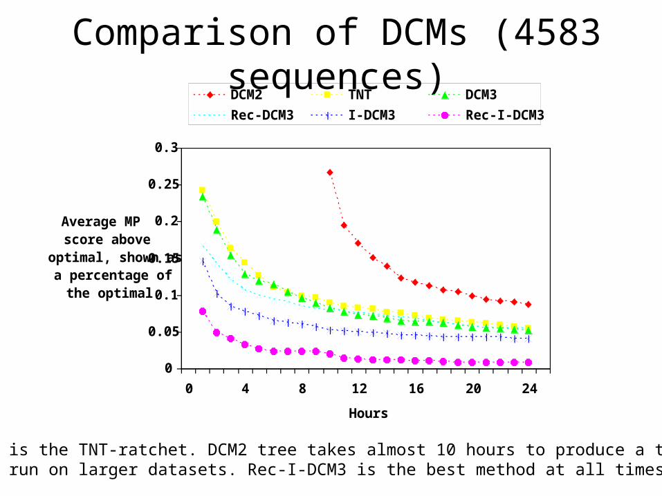
Comparison of DCMs (4583 sequences)

Base method is the TNT-ratchet. DCM2 tree takes almost 10 hours to produce a tree and is too slow to run on larger datasets. Rec-I-DCM3 is the best method at all times.

0

0.05

0.1

0.15

0.2

0.25

0.3

0 4 8 12 16 20 24

Hours

Average MP score above

optimal, shown as a percentage of

the optimal

DCM2 TNT DCM3

Rec-DCM3 I-DCM3 Rec-I-DCM3

Comparison of DCMs (13,921 sequences)

Base method is the TNT-ratchet. Note the improvement in DCMs as we move from the defaultto recursion to iteration to recursion+iteration. On very large datasets Rec-I-DCM3 gives significant improvements over unboosted TNT.

0

0.05

0.1

0.15

0.2

0.25

0.3

0.35

0.4

0 4 8 12 16 20 24

Hours

Average MP score above

optimal, shown as a percentage of

the optimal

TNT DCM3 Rec-DCM3 I-DCM3 Rec-I-DCM3

Rec-I-DCM3 significantly improves performance

Comparison of TNT to Rec-I-DCM3(TNT) on one large dataset

0

0.02

0.04

0.06

0.08

0.1

0.12

0.14

0.16

0.18

0.2

0 4 8 12 16 20 24

Hours

Average MP score above

optimal, shown as a percentage of

the optimal

Current best techniques

DCM boosted version of best techniques

Rec-I-DCM3(TNT) vs. TNT(Comparison of scores at 24 hours)

Base method is the default TNT technique, the current best method for MP. Rec-I-DCM3 significantly improves upon the unboosted TNT by returning trees which are at most 0.01% above optimal on most datasets.

00.010.020.030.040.050.060.070.080.090.1

Average MP score above

optimal at 24 hours, shown as a

percentage of the optimal

1 2 3 4 5 6 7 8 9 10

Dataset#

TNT Rec-I-DCM3

Observations

• Rec-I-DCM3 improves upon the best performing heuristics for MP.

• The improvement increases with the difficulty of the dataset.

DCMs• DCM for NJ and other distance methods produces

absolute fast converging (afc) methods• DCMs for MP heuristics • DCMs for use with the GRAPPA software for whole

genome phylogenetic analysis; these have been shown to let GRAPPA scale from its maximum of about 15-20 genomes to 1000 genomes.

• Current projects: DCM development for maximum likelihood and multiple sequence alignment.

Acknowledgements

• NSF• The David and Lucile Packard Foundation• The Program in Evolutionary Dynamics at Harvard• The Institute for Cellular and Molecular Biology at UT-

Austin• Collaborators: Usman Roshan, Bernard Moret, and Tiffani

Williams

See http://www.phylo.org and http://www.cs.utexas.edu/~tandy for more info