dislocation–obstacle interactions at the atomic level

CHAPTER 88

Dislocation–Obstacle Interactions at theAtomic Level

D.J. BACON

Department of Engineering, The University of Liverpool, Brownlow Hill, Liverpool L69 3GH, UK

Y.N. OSETSKY

Materials Sciences and Technology, ORNL, Oak Ridge, TN 37831, USA

and

D. RODNEY

Science et Ingenierie des Materiaux et Procedes, INP Grenoble, CNRS/UJF, Domaine Universitaire,Boıte Postale 46, 38402 Saint Martin d’Heres, France

r 2009 Elsevier B.V. All rights reserved Dislocations in Solids1572-4859, DOI: 10.1016/S1572-4859(09)01501-0 Edited by J. P. Hirth and L. Kubin

Contents

1. Introduction 42. Structure of models used to simulate dislocations at the atomic level 8

2.1. Rigid boundary model 82.2. Flexible boundary model 92.3. Periodic array model 10

2.3.1. Formal description of creating periodicity 102.3.2. Model for an edge dislocation 122.3.3. Model for a screw dislocation 13

2.4. Boundary conditions in the z-direction and loading techniques 152.5. Restrictions on model parameters 172.6. Other practical issues 19

3. Dislocation glide in pure metals and solid solutions 213.1. Glide in pure crystals 21

3.1.1. Glide at 0 K: the Peierls stress 213.1.2. Glide at finite temperature 233.1.3. Comparison with experiment 26

3.2. Glide in solid solutions 263.2.1. Background 263.2.2. Substitutional solute atoms 273.2.3. Interstitial solute atoms 323.2.4. Extension to microscopic models 35

4. Voids and precipitates 354.1. Introduction 354.2. Edge dislocation–obstacle interaction at T ¼ 0 K 37

4.2.1. Voids 374.2.2. Precipitates 434.2.3. Comparison of atomistic and continuum results at 0 K 45

4.3. Temperature effects for voids and precipitates 484.4. Bubbles and loose clusters of vacancies 554.5. Conclusions 56

5. Obstacles having dislocation character 575.1. Dislocation loops and SFTs 575.2. Classification of main reactions 59

5.2.1. Reaction R1: the obstacle is crossed by the dislocation and both are unchanged 595.2.2. Reaction R2: the obstacle is crossed and modified and the dislocation

is unchanged 595.2.3. Reaction R3: partial or full absorption of the obstacle by an edge

dislocation that acquires a double superjog 595.2.4. Reaction R4: temporary absorption of part or the entire obstacle into

a helical turn on a screw dislocation 605.2.5. Other reactions 60

5.3. Loops in FCC metals 615.3.1. Perfect interstitial loops 615.3.2. Interstitial Frank loops 62

5.4. Interstitial loops in BCC metals 665.4.1. ½/1 1 1S loops 665.4.2. /1 0 0S loops 705.4.3. Comparison of obstacle strength for voids and loops in iron 75

5.5. Stacking fault tetrahedra 765.5.1. Particular reactions 765.5.2. Other cases 80

5.6. Conclusions 826. Concluding remarks 83Acknowledgements 85References 85

1. Introduction

The techniques of atomic-scale simulation by computer offer ways of investi-gating properties of crystal defects that are not usually open to direct study byexperiment. Some have been in use for over 40 years and have provided importantinformation on the atomic structure and energy of crystalline defects. This chapteris concerned with dislocation–obstacle interactions that resist the glide ofdislocations in metals and hence increase the applied stress necessary to causeplastic deformation. Computer simulation of the atomic mechanisms involved inthis area of materials science is fairly recent and the aim of this chapter is tohighlight the understanding that has been achieved over the past decade. A recenthandbook [1] provides a comprehensive introduction to many aspects of modellingat both the atomic and continuum scales. It includes descriptions of methods andexamples of codes for a variety of techniques. We have tried to avoid unnecessaryoverlap except inasmuch that a clear description of the methods that have led to theresults we present is required in order that their strength and weakness can beappreciated.

We assume a prior knowledge of basic properties of dislocations, such as theBurgers vector, b; their edge, screw or mixed character; their glide (or slip) plane;the process of cross-slip; consequences of dissociation into partials; and the form ofb of perfect dislocations in body-centred cubic (BCC) and face-centred cubic (FCC)metals, i.e. ½/1 1 1S and ½/1 1 0S, respectively. (See Ref. [2] for an introductionand Refs [3,4] for more advanced and detailed presentations.) We do not go intodetail about the atomic structure of dislocation cores: recent reviews of progress inmodelling core structure in different metals and the influence of core structure ondislocation motion are to be found in Refs [5,6]. Nor do we study effects of grain orinterphase boundaries on dislocation properties and behaviour, for the materialsconsidered here are single crystals: simulation of boundary effects in nanocrystalsand other materials are discussed in Ref. [7].

In the multiscale framework for simulating the properties of dislocations inmetals, there are three distinct spatial scales, each involving distinct methods. Thefinest scale uses ab initio (first principles) calculations in which Schrodinger’sequation for interacting electrons is used to compute the position of atoms [8]. It isrestricted to a few hundred atoms at most and is therefore limited to the core regionaround a dislocation. The coarsest scale is the continuum, in which dislocations aretreated as though in an elastic, rather than atomic, medium. The distortion fieldproduced by a long dislocation varies inversely with distance and is thus long-ranged, and many of the important properties arising from this, such as stress, strainand strain energy, can be modelled using linear elasticity. Indeed, most of theapplications of dislocation theory over the past 70 years have been based on this [2–4].

Modern approaches to continuum-scale computer simulation of dislocations are notdealt with here. (For a broad introduction see Ref. [1].)

Atomic-scale simulation treated in this chapter sits between the ab initio andcontinuum scales. It uses model sizes that are large enough to allow for the maineffects of the distortion field, but also provides full resolution of the atomicstructure of the dislocation core and the obstacles a dislocation may encounter asit moves under external loading. Although the strain energy of a dislocation isaffected by the finite size of the atomic model, its core properties (structure,energy), and therefore its short-range interactions with other defects, are lesssensitive and can be described with acceptable accuracy. This can be tested bysimulating systems of increasing size in order to reach convergence of results withthe desired accuracy. The size is usually limited for the practical reason that thecomputing (CPU) time required is proportional to the number of atoms.

The need to achieve results in reasonable time limits atomic-scale modelling intwo other ways. First, the CPU time per atom is determined by the time needed tocompute the forces between, and energy of, atoms using an interatomic potential.Thus, to minimise the CPU time, the potential should have a range as short aspossible. The potentials currently used in the field are empirical potentials obtainedby different realisations of the Embedded Atom Model (EAM) [9]. Their empiricalparameters are based typically on fits to properties of the metal such as elasticconstants, phonon spectra, cohesive energy, stacking fault energy, and surface andpoint defect energies, and, increasingly frequently, to ab initio data. For reviews seeRef. [8].1

Second, the total CPU time is proportional to the number of ‘iterations’ requiredto complete the simulation. ‘Iterations’ here has one of two meanings, depending onthe simulation method. In molecular statics (MS), a crystal at temperature T ¼ 0 Kis modelled, i.e. the kinetic energy of the atoms is maintained equal to zero, andthe system achieves equilibrium when the potential energy, computed by summingthe interatomic potential energy of the atoms minus the work of forces appliedto the system, is minimised. This state is found from a trial starting configurationby a series of iterations in which the atoms are moved repeatedly. (See Ref. [1]for examples.) In molecular dynamics (MD), kinetic energy is not zero andat equilibrium the average kinetic energy per atom equals 3kBT/2, where kB isthe Boltzmann constant. At a given time t, the acceleration of every atom iscalculated from the force on it due to its neighbours using Newton’s second law(force ¼ mass� acceleration). This equation of motion is solved numerically for allatoms to predict their position at time (tþDt), where Dt is the MD time-step, e.g.Refs [1,10]. This procedure is repeated to enable the trajectory of atoms to befollowed for as long as is necessary to complete the process under investigation, thenumber of iterations in this case being the number of time-steps. To maintainaccuracy, Dt is typically of the order of one to a few femtoseconds (1 fs ¼ 10�15 s).

1 For the references to the potentials used for the results presented in this chapter, the reader is referredto the original papers we cite.

y1 Dislocation–Obstacle Interactions at the Atomic Level 5

We give a few examples of model size and computing resource required inSection 2. For the moment, it is sufficient to bear in mind that the models of interesthere contain typically from a few hundred thousand to a few million atoms. Size inthis range is usually sufficient for treatment of the elastic field of one dislocation andfor it to move and interact with other defects without severe restriction by themodel boundary conditions. In simulation of atomic dynamics by MD, the numberof time-steps that can be accomplished within a reasonable CPU time is typically inthe range 105–107, so that the total simulated time is of the order of nanoseconds(1 ns ¼ 10�9 s). Thus, the spatial and time scales of the work reviewed here arenanoscale.

A model for simulating dislocation–obstacle interactions on these scales shouldsatisfy the following criteria.

(a) It should not artificially constrain the dislocation core structure and itshould ensure that the displacement, u, of the atoms from their perfectcrystal sites exhibits the discontinuity that defines the dislocation withBurgers vector b, i.e.

b ¼

Idu; (1)

where the integral encircles the dislocation line.(b) It should be large enough to permit accurate simulation of the effects of the

elastic distortion field of the dislocation.(c) It should allow for dislocation motion to occur as a result of application of

external action in the form of stress or strain: this motion should not berestricted by the model boundaries.

(d) It should permit simulation of either static (T ¼ 0 K) or dynamic (TW0 K)conditions.

(e) Methods should be incorporated for visualising the atoms in the vicinity ofthe dislocation core and obstacle during the process under investigation.

Computer models that satisfy these criteria are described in the Section 2, withemphasis on a method that allows the construction of an infinite, periodic glideplane for the mobile dislocation. This model is applied in the following sections forsimulation of the interaction of dislocations with crystalline defects. Practical limitson model size restrict the size of these defects to a few nanometres.

Much of the research presented here has been driven by the need to investigatethe effect of radiation on the mechanical behaviour of metals in current and futurenuclear power systems, for the defects of concern are of the order of a nanometrein size and their interactions with dislocations cannot be observed directly byexperiment. The core components of reactors are subjected to irradiation by a fluxof fast neutrons produced by the nuclear reaction (e.g. Ref. [11]). The neutronsinduce damage in metals that can change their mechanical properties. Indeed, fastneutrons (as well as ions) produce localised regions of defects by the displacement-cascade process, in which an atom is given sufficient energy by an irradiatingparticle that it can displace many of its neighbours in an avalanche of collisions.

6 D.J. Bacon et al. Ch. 88

Displaced atoms that do not return to their lattice sites become self-interstitialatoms (SIAs), mainly at the periphery of a cascade, and a corresponding number ofsites are left vacant in the central region (see Ref. [12] and references cited therein).A substantial fraction of these defects form clusters with their own kind, eitherduring the cascade process itself, which has a lifetime B10 ps, or after diffusion inthe material. SIAs usually cluster as tightly packed planar arrays of crowdions thatare nascent dislocation loops with perfect Burgers vector parallel to the crowdionaxis, i.e. b ¼ ½/1 1 0S in FCC, ½/1 1 1S or /1 0 0S in BCC and 1/3/1 1 �2 0S inHCP (e.g. Refs [13–15]). Faulted loops with b ¼ 1/3/1 1 1S also form in FCCmetals. Vacancies cluster in the form of loops or, in FCC metals, in a specificdissociated structure called a stacking fault tetrahedron (SFT). Depending onthe metal and irradiation conditions, they can also agglomerate to form voidsand when He is present, as a result of either transmutation or direct injection,He-filled bubbles can arise. Plasticity is strongly affected by such clustered defects.The yield stress is usually increased, the work-hardening rate and ductility reducedand flow localisation by dislocation channelling can occur at high levels of clusterdensity (e.g. Refs [16–18]). In the latter case, deformation is inhomogeneous andlocalised in bands of intense plastic shear that appear to be clear of irradiationdefects when observed in a transmission electron microscope (TEM) after thedeformation, e.g. Ref. [16].

Linear elasticity theory can provide a description of dislocation interactionwith obstacles. However, approximations have to be made for processes thatare controlled by atomic mechanisms, in particular when the interaction involvesdirect contact between the dislocation and obstacle, for the core of the dislocationis involved in the interaction process. On the other hand, the defects producedunder irradiation have sizes in the nanometre range and since their density ishigh, B1023 m�3 (e.g. Refs [19–21]), their average separation is on the order ofa few tens of nanometres. They are amenable to atomic-scale simulations. The aimof the research presented below has been to study both the elementary mechanismsof interaction between one dislocation of definite character (edge or screw)with one particular defect and measure directly from the simulation the pinningeffect due to the defect on the dislocation. In a multiscale approach, suchinformation can be then used in dislocation dynamics (DD) simulations tosimulate the more statistical problem of the glide of dislocations in populations ofdefects [22].

After a description of the methods in Section 2, we consider in Section 3 theinteraction of dislocations with the crystal itself (exemplified by the Peierls stressand DD) and solute atoms (interaction that controls solid solution hardening(SSH)). We then review interaction with voids and precipitates in Section 4.Obstacles with dislocation character are considered in Section 5, i.e. dislocationloops and SFTs. Because of the possibility of dislocation reactions, more complexand varied reactions are observed with this category of obstacle. The casesthat have been studied extensively are those for FCC and BCC metals: HCP metalshave received far less attention, mainly because of the absence of reliableinteratomic potentials suited for the study of dislocations.


2. Structure of models used to simulate dislocations at the atomic level

2.1. Rigid boundary model

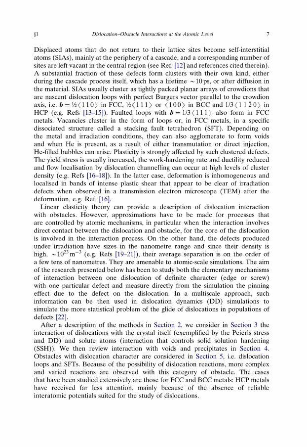
The simplest approach, which was used in early atomic-level modelling ofdislocations [23–29], is to generate the atom coordinates of a perfect crystal ofthe required structure, orientation and size and impose on them the dislocationdisplacement field given by linear elasticity theory. In order to prevent a return tothe perfect crystal state when relaxation occurs, boundary conditions have to beapplied to the model. This is achieved by creating a layer of atoms (FR) fixedin their unrelaxed position around the outside of the inner region of mobileatoms (MR), i.e. rigid boundary conditions (RBCs) are used. This arrangement isshown schematically in Fig. 1(a) as a cross-section of a cylinder containing anedge dislocation. Invariance of the dislocation field along its line allows periodicityalong the y-axis and this is readily achieved by adding the translation7Ly, i.e. thelength of the model in the y direction, to the y coordinate of atoms in region MR.The thickness of the rigid and periodic layers has to be larger than the range of theinteratomic potential in order that atoms in the inner region have a full set ofneighbours.

The RBC method with this configuration has been used to study dislocationproperties such as core structure and energy, and led to valuable insights in earlywork on the core properties of screw dislocations in BCC metals [29,30]. However,region MR must be sufficiently large for relaxation of the atoms in the vicinity ofthe dislocation core to be unrestricted by the rigid boundaries. This condition isparticularly important when the dislocation can dissociate, i.e. the core is wide.For instance, the dissociation width of a screw dislocation in a model of Ni saturates

Fig. 1. (a) Representation of rigid boundary model showing regions of fixed (FR) and mobile (MR)atoms. (b) Representation of flexible boundary model showing the continuum (CR), Green’s function

(GFR) and mobile (MR) atom regions.


to the true value (B2 nm) only when the distance from the centre of the dislocationcore to the fixed boundary is W6.3 nm (B25b) [31].

The initiation of dislocation motion in a RBC model can be studied by applyingincreasing homogeneous shear strain, e, in small increments and relaxing theposition of the mobile atoms at each increment. The critical value, eP, at which thedislocation moves from its initial position gives the Peierls stress tP ¼ GeP, where Gis the elastic shear modulus. However, the rigid boundaries oppose this motionbecause their atom coordinates correspond to the initial position of the dislocation.This produces a configuration force on the dislocation that increases as it movesnearer the boundary. This leads to an overestimation of the Peierls stress [32],which can be up to almost an order of magnitude in low Peierls stress crystals(see, e.g. Ref. [31]). Also, stress cannot be applied with this model.

2.2. Flexible boundary model

Green’s function boundary conditions (GFBCs) offer a more sophisticatedtechnique, for they allow flexible boundaries to be simulated according to theelastic and/or lattice properties of the crystal, thereby enabling the boundariesto distort in response to the dislocation. (The displacement at point x due to aninfinitesimal force F at point xu is u ¼ G(x� xu)F, where G is the Green’s function.)Two-dimensional (2D) [33] and three-dimensional (3D) [31,34,35] realisations ofGFBCs have been suggested and applied in studies of cracks and dislocations.

The simulation cell consists of three regions shown schematically in Fig. 1(b). Thelinear elastic displacement field of the dislocation is initially applied to the wholemodel, after which atoms in region MR are relaxed with their forces derived froman interatomic potential, whilst their neighbours in the Green’s function region(GFR) and continuum region (CR) are held fixed. This results in non-zero forces onatoms in the GFR. These forces are then relaxed by displacing atoms in both theGFR (displacements calculated from the lattice Green’s function) and the outer CR(displacements calculated via the elastic Green’s function). The process is repeateduntil forces in the GFR fall below a chosen value. In practice, up to 10 iterationsmay be necessary to achieve reasonable accuracy for dislocation core structure andenergy. For details see Refs [31,35].

The GFBC technique has several advantages over simpler RBC methods.It allows a significant reduction in the minimum size of the inner region requiredto reproduce the correct core structure and Peierls stress [31]. Also, for the samenumber of atoms in the inner region, the dislocation can move further withoutstrong interference from the boundaries, although a dislocation–boundary distanceof typically B15–20a0 is required for reasonable results. The method is particularlyattractive for simulations where the number of atoms has to be kept small becausecalculation of interatomic forces is computationally time-consuming, e.g. ab initio ormany-body interactions [36–38]. However, self-consistent convergence with GFBCsrequires many force calls and calculations of long-range Green’s functions, andresults in lower computational efficiency than the RBC method for problems

y2.2 Dislocation–Obstacle Interactions at the Atomic Level 9

involving a large number of atoms. Examples of two simulations are given inSection 2.6.

2.3. Periodic array model

The GFBC model is not suited to simulation of dynamic conditions (temperatureTW0 K). Both the RBC and GFBC methods suffer from additional limitations.First, as already mentioned, the boundaries are not transparent and the dislocationcannot travel over long distances. Second, they are compatible with application ofonly external strain and not stress: when the dislocation moves under applied strain,the stress, which arises from the elastic part of the strain only, decreases andconstant applied stress simulations cannot be performed. A way to circumvent theseproblems is to use a periodic array of dislocations (PAD), as proposed initially byDaw et al. [39]. The simulated crystal containing an initially straight dislocation hasPBCs in the dislocation glide plane, i.e. not only in the dislocation line direction (y)but also in the glide direction (x), thereby creating an infinite array of infinitelylong, parallel dislocations. The dislocation still experiences model-size effects dueto interaction with its periodic images but the effect is constant throughoutthe simulation cell, irrespective of the dislocation position relative to the cellboundaries. Effects of external loading can be studied by applying either stress orstrain, and the dislocation can glide over a long (in principle, infinite) distancebecause of transparency associated with PBCs. Models based on a PAD arecomputationally efficient for a large number of atoms and, as will be shown later,can be used for not only qualitative but also quantitative studies of DD andmechanisms, and for parameterisation of the processes linking the atomic andcontinuum approaches.

To illustrate the method, we consider first in Section 2.3.1 a general approach forcreating periodicity in the glide plane of a dislocation and then present twoparticular examples of edge (Section 2.3.2) and screw dislocations (Section 2.3.3).Treatment of the BCs in the direction normal to the glide plane and ways in whichexternal loading is applied are discussed in Section 2.4.

2.3.1. Formal description of creating periodicityThe following approach provides a formal prescription for generating PBCsalong both the dislocation line (y-axis) and its direction of motion (x-axis) for adislocation of any character. It follows from the fact that the Burgers vector b of aperfect dislocation is a translation vector of the lattice, usually the shortest latticevector. It can therefore be described as the difference between two other latticevectors. The prescription is as follows.

(i) Construct two half crystals, which we label l (upper) and m (lower), with thesame orientation.

(ii) Select lattice translations vectors tl and tm in l and m such that b ¼ (tl� tm).


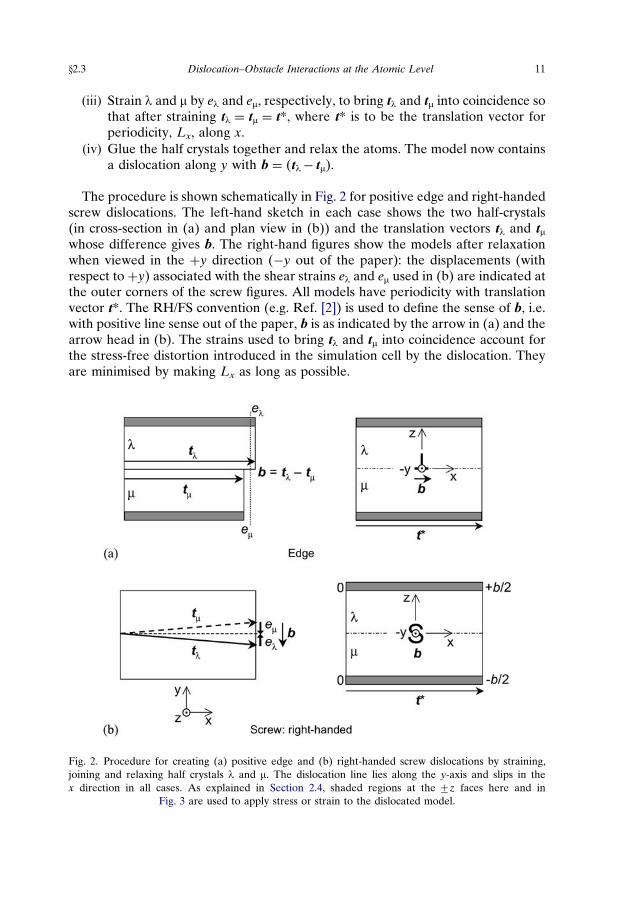
(iii) Strain l and m by el and em, respectively, to bring tl and tm into coincidence sothat after straining tl ¼ tm ¼ t*, where t* is to be the translation vector forperiodicity, Lx, along x.

(iv) Glue the half crystals together and relax the atoms. The model now containsa dislocation along y with b ¼ (tl� tm).

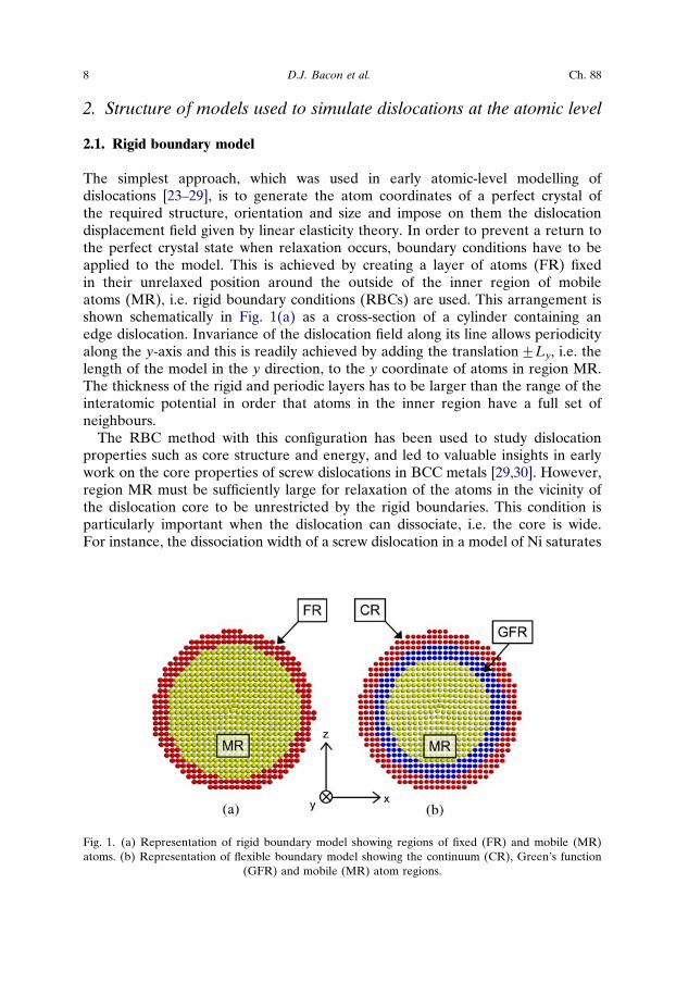
The procedure is shown schematically in Fig. 2 for positive edge and right-handedscrew dislocations. The left-hand sketch in each case shows the two half-crystals(in cross-section in (a) and plan view in (b)) and the translation vectors tl and tmwhose difference gives b. The right-hand figures show the models after relaxationwhen viewed in the þy direction (�y out of the paper): the displacements (withrespect to þy) associated with the shear strains el and em used in (b) are indicated atthe outer corners of the screw figures. All models have periodicity with translationvector t*. The RH/FS convention (e.g. Ref. [2]) is used to define the sense of b, i.e.with positive line sense out of the paper, b is as indicated by the arrow in (a) and thearrow head in (b). The strains used to bring tl and tm into coincidence account forthe stress-free distortion introduced in the simulation cell by the dislocation. Theyare minimised by making Lx as long as possible.

Fig. 2. Procedure for creating (a) positive edge and (b) right-handed screw dislocations by straining,joining and relaxing half crystals l and m. The dislocation line lies along the y-axis and slips in thex direction in all cases. As explained in Section 2.4, shaded regions at the 7z faces here and in

Fig. 3 are used to apply stress or strain to the dislocated model.


A similar method can be used to create PAD models for interfacial dislocationssuch as twinning dislocations. In this case, l and m have different orientation andthe dislocation forms a step in the twin boundary ([40], see p. 173 of Ref. [2]).Nevertheless, by appropriate choice of tl and tm such that (tl� tm) equals b of thetwinning dislocation, periodicity can be exploited to study the long-range motion ofthe boundary (e.g. Ref. [41]).

Practicalities for the edge and screw dislocations in a single crystal are consideredin more detail in the following two sections.

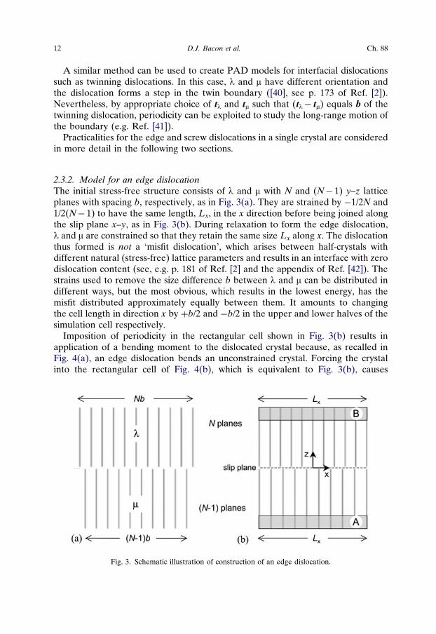
2.3.2. Model for an edge dislocationThe initial stress-free structure consists of l and m with N and (N� 1) y–z latticeplanes with spacing b, respectively, as in Fig. 3(a). They are strained by �1/2N and1/2(N� 1) to have the same length, Lx, in the x direction before being joined alongthe slip plane x–y, as in Fig. 3(b). During relaxation to form the edge dislocation,l and m are constrained so that they retain the same size Lx along x. The dislocationthus formed is not a ‘misfit dislocation’, which arises between half-crystals withdifferent natural (stress-free) lattice parameters and results in an interface with zerodislocation content (see, e.g. p. 181 of Ref. [2] and the appendix of Ref. [42]). Thestrains used to remove the size difference b between l and m can be distributed indifferent ways, but the most obvious, which results in the lowest energy, has themisfit distributed approximately equally between them. It amounts to changingthe cell length in direction x by þb/2 and �b/2 in the upper and lower halves of thesimulation cell respectively.

Imposition of periodicity in the rectangular cell shown in Fig. 3(b) results inapplication of a bending moment to the dislocated crystal because, as recalled inFig. 4(a), an edge dislocation bends an unconstrained crystal. Forcing the crystalinto the rectangular cell of Fig. 4(b), which is equivalent to Fig. 3(b), causes

Fig. 3. Schematic illustration of construction of an edge dislocation.


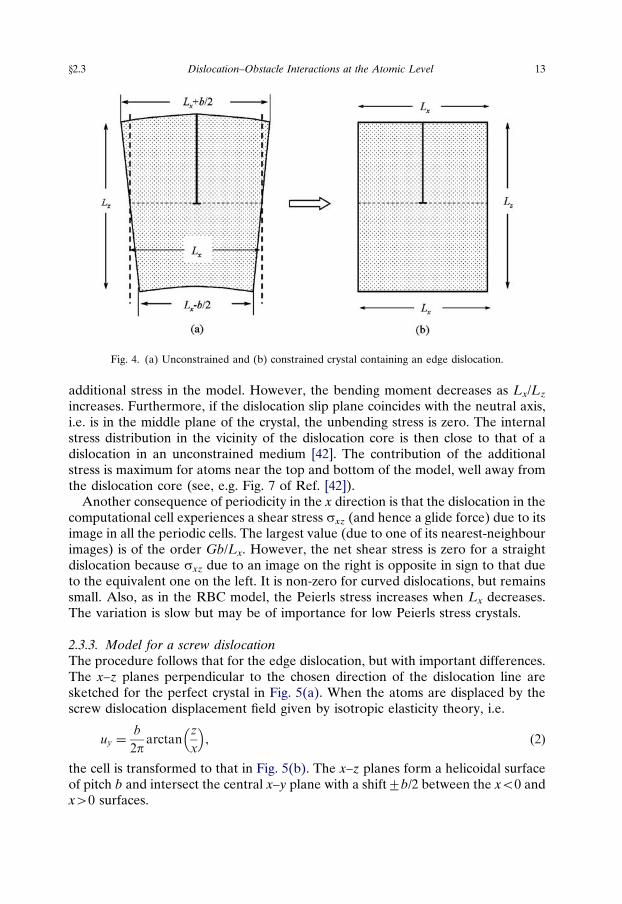
additional stress in the model. However, the bending moment decreases as Lx/Lz

increases. Furthermore, if the dislocation slip plane coincides with the neutral axis,i.e. is in the middle plane of the crystal, the unbending stress is zero. The internalstress distribution in the vicinity of the dislocation core is then close to that of adislocation in an unconstrained medium [42]. The contribution of the additionalstress is maximum for atoms near the top and bottom of the model, well away fromthe dislocation core (see, e.g. Fig. 7 of Ref. [42]).

Another consequence of periodicity in the x direction is that the dislocation in thecomputational cell experiences a shear stress sxz (and hence a glide force) due to itsimage in all the periodic cells. The largest value (due to one of its nearest-neighbourimages) is of the order Gb/Lx. However, the net shear stress is zero for a straightdislocation because sxz due to an image on the right is opposite in sign to that dueto the equivalent one on the left. It is non-zero for curved dislocations, but remainssmall. Also, as in the RBC model, the Peierls stress increases when Lx decreases.The variation is slow but may be of importance for low Peierls stress crystals.

2.3.3. Model for a screw dislocationThe procedure follows that for the edge dislocation, but with important differences.The x–z planes perpendicular to the chosen direction of the dislocation line aresketched for the perfect crystal in Fig. 5(a). When the atoms are displaced by thescrew dislocation displacement field given by isotropic elasticity theory, i.e.

uy ¼b

2parctan

z

x

� �, (2)

the cell is transformed to that in Fig. 5(b). The x–z planes form a helicoidal surfaceof pitch b and intersect the central x–y plane with a shift7b/2 between the xo0 andxW0 surfaces.

Fig. 4. (a) Unconstrained and (b) constrained crystal containing an edge dislocation.


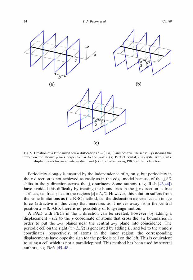
Periodicity along y is ensured by the independence of uy on y, but periodicity inthe x direction is not achieved as easily as in the edge model because of the7b/2shifts in the y direction across the 7x surfaces. Some authors (e.g. Refs [43,44])have avoided this difficulty by treating the boundaries in the 7x direction as freesurfaces, i.e. free space in the regions |x|WLx/2. However, this solution suffers fromthe same limitations as the RBC method, i.e. the dislocation experiences an imageforce (attractive in this case) that increases as it moves away from the centralposition x ¼ 0. Also, there is no possibility of long-range motion.

A PAD with PBCs in the x direction can be created, however, by adding adisplacement 7b/2 to the y coordinate of atoms that cross the 7x boundaries inorder to put the x–z planes near the central x–y plane into coincidence. Theperiodic cell on the right (xWLx/2) is generated by adding Lx and b/2 to the x and ycoordinates, respectively, of atoms in the inner region: the correspondingdisplacements have opposite sign for the periodic cell on the left. This is equivalentto using a cell which is not a parallelepiped. This method has been used by severalauthors, e.g. Refs [45–48].

Fig. 5. Creation of a left-handed screw dislocation (b ¼ [0, b, 0] and positive line sense �y) showing theeffect on the atomic planes perpendicular to the y-axis. (a) Perfect crystal, (b) crystal with elastic

displacements for an infinite medium and (c) effect of imposing PBCs in the x-direction.


In both the edge and screw models, shifts7b/2 are added across the7x surfacesin the Burgers vector direction. As seen above, in the edge case, it amounts to anexpansion of the cell along with a bending moment. In the screw case, it results inshearing the cell. Also, inspection of Fig. 5(b) reveals that the x–z planes are notvertical in the7x surfaces but are inclined with angles of opposite sign in the xo0 andxW0 surfaces. Imposition of PBCs forces these planes to become vertical, as shown inFig. 5(c), which is equivalent to applying a torque in the7x surfaces. The influence ofthis torque is difficult to evaluate but it decreases with the ratio Lz/Lx. A PAD modelfor a mixed dislocation can be created by mixing the edge and screw shifts.

2.4. Boundary conditions in the z-direction and loading techniques

Boundary conditions at the7z surfaces are important because action due to externalloading is applied there. It is clear from Figs 3(b) and 5(c) for the edge and screwdislocations, respectively, that PBCs cannot be used, and free BCs can only beemployed when external load effects are not of interest. Two choices for the 7zboundaries are possible: either rigid or pseudo-free. In the former case, an atomicblock (of thickness exceeding the range of the interatomic potential) is created ateach boundary with atoms fixed in their initial, strained position [42]. These arerepresented by the shaded regions in Figs 2 and 3. A second possibility is to createfree space in the regions |z|WLz/2. The7z surfaces can be either fully free [49,50] orconstrained to 2D dynamics by allowing surface atom motion only in directions x andy [51,52]. This condition is compatible only with stress-controlled simulations, whereasrigid boundaries can be used for either stress- or strain-controlled simulations.

Consider the model shown schematically in Fig. 3. A dislocation lies along the yaxis perpendicular to the paper and was formed by the process described inSection 2.3, wherein atoms in the inner region, MR, are free to move in static ordynamic simulations. Blocks A and B at the7z surfaces are used to apply externalaction and atoms in them are either fixed in their initial position relative to eachother using RBCs or free to move in any direction using free boundary conditions.The primary glide plane is the plane z ¼ 0. The glide force per unit length ofdislocation line is given by F ¼ tb, where t is the component of stress resolved onthe glide plane in the direction of b, i.e. sxz and syz for the edge and screw,respectively. F due to external action can be generated in two ways, as follows.

(i) Shear strain e applied. Either one or both of the blocks A and B can be usedto apply a strain, but for simplicity we assume that A is fixed and thedislocation moves when actions are applied to B. Application of sheardisplacement u ¼ [ux, uy, 0] produces shear strain components

�xz ¼ux

Lzand �yz ¼

uy

Lz. (3)

Rigid boundaries are required for A and B in order to maintain thisstrain during the relaxation of the mobile atoms. The corresponding appliedshear stress components sxz and syz, which create a glide force on the edge


and screw components of the dislocation, respectively, are calculated fromthe total force FB ¼ ½FB

x ;FBy ;F

Bz � on all the atoms in B (which at equilibrium

is equal to the total force, FA, on A) by the relations:

sxz ¼ �FBx

Axyand syz ¼ �

FBy

Axy, (4)

where Axy ¼ LxLy is the x–y cross-section area of the crystallite of mobileatoms.

(ii) Shear stress t applied. For stress loading, a shear force F ¼ [Fx, Fy, 0] isapplied either to the atoms in block B, which is allowed to move rigidly whileblock A is held fixed, or as F applied to B and �F to A if A and B are eitherfree or both allowed to move rigidly. The force components are chosen suchthat the required stresses sxz ¼ Fx/Axy and syz ¼ Fy/Axy are applied. Theshear strain components resulting from the applied stress are calculated fromu as in eq. (3). In the case of free boundary conditions, ux and uy are theaverage differences of displacement of atoms in A and B.

Note that in order to apply a strain, e.g. exz, only the average difference indisplacement in direction x between blocks A and B has to be fixed while theatomic displacements in directions y and z can be unconstrained. As a result,another possibility to apply a strain is to constrain only the position of thecentre of gravity of the blocks A and B and not the position of every atom[53]. This is achieved by subtracting at every simulation step the averageforce on a block from the forces on atoms within it, i.e. for atoms in B,Fx ¼ Fx�/FxS

B and similarly for atoms in A.There are several differences between application of external action for

simulation by MS (T ¼ 0 K) and MD (TW0 K). In MS, increasing strain canbe applied in increments, with potential energy minimisation performed afterevery increment. In case (ii) the potential energy is the internal energycomputed with the interatomic potential from the position of the atoms minusthe work of the applied stress (¼F(uB

� uA)). With free boundaries, uA anduB are the average displacements in the two blocks. In MD simulations, bothforms of external loading can be used. For scenario (i), the model crystal hasto be equilibrated at the chosen temperature and shear strain then applied ata given rate by imposing velocity v ¼ [vx, vy, 0] on B, with stress calculatedfrom FB (eq. (4)). In scenario (ii), constant shear stress or stress rate canbe applied by imposing constant or increasing shear force F ¼ [Fx, Fy, 0] afterequilibration. With RBCs, B is free to move under the combined influence ofexternal force F and internal force FB and has to be treated as a separatesuper-particle of mass MB with an equation of motion coupled with thoseof all mobile atoms. The corresponding shear strain rate at any instant iscalculated from v/Lz. (Again, with free boundary conditions v is the averageatomic velocity in B.) A feature of PAD models pointed out in Ref. [42] isthat dislocation motion obeys the Orowan relationship between mobiledislocation density, rD, dislocation velocity, vD, and the resulting plastic shear


strain rate (see, e.g. Ref. [2]). After integration over time, t, with constant rD,this law takes the form

� ¼

ZvDbrDdt ¼ �xbrD ¼ �x

b

LxLz, (5)

where �x is the mean distance of dislocation motion.

2.5. Restrictions on model parameters

Available computing power limits the size and complexity of atomic models thatcan be simulated. The total CPU time required is proportional to the product of thenumber of atoms and the number of MS relaxation iterations or MD time-steps.With the models presented in Sections 2.1–2.3, the boundary conditions in the glidedirection result in forces on the dislocation due to either periodic or imagedislocations, but their influence can be made minimal if the model is large enough.The PAD method is particularly favourable because the periodic images remainat constant distance from the dislocation. Also, even with scalar computing, it ispossible to simulate cell volumes that correspond to large but realistic dislocationdensity rD. For example, a model of a metal with dimensions Lx ¼ 25 nm,Ly ¼ 40 nm, Lz ¼ 25 nm containing one dislocation has rD ¼ 1/LxLz ¼ 1.6� 1015

m�2, which is within the range found experimentally in heavily cold-worked metals.It contains approximately 2,000,000 mobile atoms, a number that can be simulatedeasily with a scalar computer and empirical interatomic potentials. With oneobstacle to dislocation motion in the cell, i.e. a periodic obstacle spacing of 40 nm,the model is representative of many real situations. By using parallel computing,rD can be reduced by at least an order of magnitude.

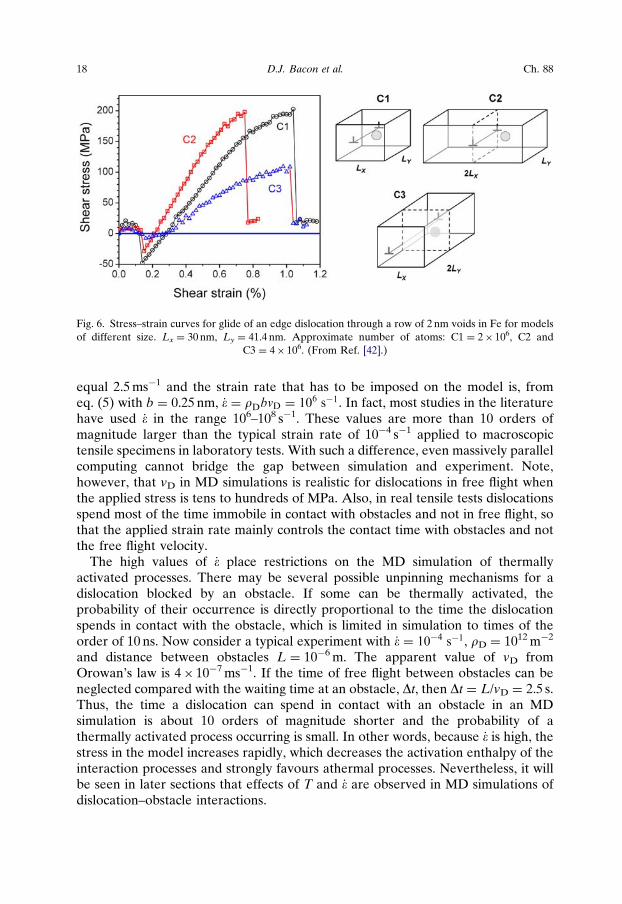
To illustrate the suitability of models of this size, Fig. 6 contains shear stress versusshear strain plots for MS simulation of glide of an edge dislocation through a periodicrow of 2 nm voids in Fe at T ¼ 0 K [42]. (Here and throughout the text, we use Fe todenote a-Fe, the stable BCC phase of pure iron below 911 1C at atmosphericpressure.) The plots correspond to three models of different size, each containing onevoid. (The form of these plots is explained in Section 4.2.1.) The critical (maximum)shear stress is seen to be independent of Lx (C1 and C2) and to be halved when Lz isdoubled (C3), as expected from elasticity theory (see Section 4.2.3, eqs (13) and (14)).The limitation on model dimensions imposed by computing power is therefore notsignificant for the problems to be discussed in later sections.

Restrictions on timescale are more serious, however, and lead to values ofplastic strain rate, _�, in MD simulations that are high compared to experiment. Toillustrate, consider glide of a dislocation across the 25� 40� 25 nm3 simulation cellabove. The maximum MD time-step required to maintain accuracy is typically inthe range 1–5 fs, depending on T, so a simulated time of 10 ns requires between 107

and 2� 106 time-steps. Assuming the computer code runs at 10�6 s of CPU time peratom per time-step, the total CPU time for the simulation is in the range 46–231days. For the dislocation to glide the distance Lx in this time, its velocity, vD, has to


equal 2.5 ms�1 and the strain rate that has to be imposed on the model is, fromeq. (5) with b ¼ 0.25 nm, _� ¼ rDbvD ¼ 106 s�1. In fact, most studies in the literaturehave used _� in the range 106–108 s�1. These values are more than 10 orders ofmagnitude larger than the typical strain rate of 10�4 s�1 applied to macroscopictensile specimens in laboratory tests. With such a difference, even massively parallelcomputing cannot bridge the gap between simulation and experiment. Note,however, that vD in MD simulations is realistic for dislocations in free flight whenthe applied stress is tens to hundreds of MPa. Also, in real tensile tests dislocationsspend most of the time immobile in contact with obstacles and not in free flight, sothat the applied strain rate mainly controls the contact time with obstacles and notthe free flight velocity.

The high values of _� place restrictions on the MD simulation of thermallyactivated processes. There may be several possible unpinning mechanisms for adislocation blocked by an obstacle. If some can be thermally activated, theprobability of their occurrence is directly proportional to the time the dislocationspends in contact with the obstacle, which is limited in simulation to times of theorder of 10 ns. Now consider a typical experiment with _� ¼ 10�4 s�1, rD ¼ 1012 m�2

and distance between obstacles L ¼ 10�6 m. The apparent value of vD fromOrowan’s law is 4� 10�7 ms�1. If the time of free flight between obstacles can beneglected compared with the waiting time at an obstacle, Dt, then Dt ¼ L/vD ¼ 2.5 s.Thus, the time a dislocation can spend in contact with an obstacle in an MDsimulation is about 10 orders of magnitude shorter and the probability of athermally activated process occurring is small. In other words, because _� is high, thestress in the model increases rapidly, which decreases the activation enthalpy of theinteraction processes and strongly favours athermal processes. Nevertheless, it willbe seen in later sections that effects of T and _� are observed in MD simulations ofdislocation–obstacle interactions.

Fig. 6. Stress–strain curves for glide of an edge dislocation through a row of 2 nm voids in Fe for modelsof different size. Lx ¼ 30 nm, Ly ¼ 41.4 nm. Approximate number of atoms: C1 ¼ 2� 106, C2 and

C3 ¼ 4� 106. (From Ref. [42].)


2.6. Other practical issues

The pros and cons of the methods reviewed here can be summarised as follows.RBC models are simple to implement and fast for even millions of atoms with short-range empirical interatomic potentials. They are convenient for core structurestudies and immobile dislocation–defect interaction simulations, but not forapplication of external stress or strain. GFBC models overcome some of thedisadvantages of rigid boundaries. They are suitable for static conditions (T ¼ 0 K)and simulations where long-range elastic effects influence dislocation corestructure and interaction energy with other defects, or when the interatomic forcecalculations are computationally expensive and the number of atoms is small. It isnot sensible to use them when the dislocation bends strongly under applied strainand sweeps a large area, for such cases require a large inner region and demandlarge computational resource because of the long-range nature of the elasticGreen’s function.

The PAD technique has been developed for use with short-range empiricalinteratomic potentials and has been applied extensively for simulation ofdislocation–obstacle interaction under a wide range of conditions, i.e. appliedstrain at T ¼ 0 K and applied strain or stress at TW0 K. It is intrinsically lessaccurate than the GFBC method, but this is more than offset by its computationalefficiency for models with up to millions of atoms. To illustrate this, consider glideof an edge dislocation of the ½[1 1 1]ð1 �1 0Þ slip system in GFBC and PAD modelsof Fe containing approximately 0.5� 106 atoms at 0 K [54]. It encounters a row of2 nm spherical voids of spacing 20 nm and, under increasing applied strain,overcomes them. (Details of this are presented in Section 4.2.1.) The dislocationshape in the glide plane at the maximum stress when the dislocation breaks away isshown in Fig. 7(a). Both shapes are identical in the vicinity of the void, but forwardmotion of the dislocation between the voids has been restricted in the GFBC modelby the boundaries, which are about 15a0 away, where a0 is the lattice parameter.The dislocation climbs in both cases by absorbing vacancies as it leaves the void,as shown in Fig. 7(b). The CPU time with the GFBC method was more than oneorder larger than with the PAD model, demonstrating that the latter offers similaraccuracy with much smaller computational resource.

A model-specific effect can arise when the PAD model is used to study thereaction of a screw dislocation with an obstacle. It will be seen in Sections 4 and 5that if the dislocation absorbs point defects from an obstacle, it acquires a helicalturn. This can glide along the dislocation line, i.e. in the direction of b, and, if L isshort and _� or t are low, it can move through a periodic boundary and reappear onthe other side of the original obstacle, thereby restoring it. The dislocation usuallychanges its slip plane by double cross-slip in this process. We do not consider thatthis simulates a real reaction.

Finally, since a strength of atomic-scale modelling is its ability to simulateprocesses in the dislocation core, it is important to visualise and identify structure inthis region. For the edge dislocation with b ¼ ½[1 1 1] in the BCC metal consideredabove, a simple analysis of atomic disregistry in the core provides satisfactory


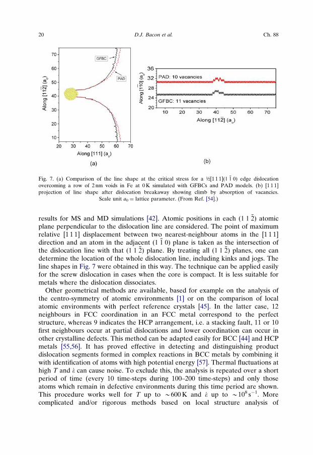
results for MS and MD simulations [42]. Atomic positions in each ð1 1 �2Þ atomicplane perpendicular to the dislocation line are considered. The point of maximumrelative [1 1 1] displacement between two nearest-neighbour atoms in the [1 1 1]direction and an atom in the adjacent ð1 �1 0Þ plane is taken as the intersection ofthe dislocation line with that ð1 1 �2Þ plane. By treating all ð1 1 �2Þ planes, one candetermine the location of the whole dislocation line, including kinks and jogs. Theline shapes in Fig. 7 were obtained in this way. The technique can be applied easilyfor the screw dislocation in cases when the core is compact. It is less suitable formetals where the dislocation dissociates.

Other geometrical methods are available, based for example on the analysis ofthe centro-symmetry of atomic environments [1] or on the comparison of localatomic environments with perfect reference crystals [45]. In the latter case, 12neighbours in FCC coordination in an FCC metal correspond to the perfectstructure, whereas 9 indicates the HCP arrangement, i.e. a stacking fault, 11 or 10first neighbours occur at partial dislocations and lower coordination can occur inother crystalline defects. This method can be adapted easily for BCC [44] and HCPmetals [55,56]. It has proved effective in detecting and distinguishing productdislocation segments formed in complex reactions in BCC metals by combining itwith identification of atoms with high potential energy [57]. Thermal fluctuations athigh T and _� can cause noise. To exclude this, the analysis is repeated over a shortperiod of time (every 10 time-steps during 100–200 time-steps) and only thoseatoms which remain in defective environments during this time period are shown.This procedure works well for T up to B600 K and _� up to B108 s�1. Morecomplicated and/or rigorous methods based on local structure analysis of

Fig. 7. (a) Comparison of the line shape at the critical stress for a ½[1 1 1]ð1 �1 0Þ edge dislocationovercoming a row of 2 nm voids in Fe at 0 K simulated with GFBCs and PAD models. (b) [1 1 1]projection of line shape after dislocation breakaway showing climb by absorption of vacancies.

Scale unit a0 ¼ lattice parameter. (From Ref. [54].)


neighbours [58] or Voronoi polyhedra analysis [59] can also be applied, but usuallyat a cost to CPU time.

3. Dislocation glide in pure metals and solid solutions

3.1. Glide in pure crystals

The basic controllers of dislocation glide are the nature of the bonding betweenatoms and the crystal structure of the metal itself [60], for they determine thearrangement of atoms in the core region of a dislocation. The mobility ofdislocations depends strongly on the ability of the core to spread. (See Refs [5,6] forrecent reviews.) If a metastable stacking fault can form on a plane by sheardisplacement between atoms, this may lead to dissociation of a dislocation withperfect b into partial dislocations separated by a fault and hence a relatively widecore. Crystal symmetry guarantees an extremum on the stacking fault energysurface (also known as the g-surface) for some slip systems in metals [61], e.g.½/1 1 0S{1 1 1} in FCC and 1/3/1 1 �2 0S(0 0 0 1) in HCP, but not others, e.g.½/1 1 1S{1 1 0} or ½/1 1 1S{1 1 2} in BCC and 1/3/1 1 �2 0Sf1 0 �1 0g in HCP.Whether or not a stable fault occurs in the latter cases depends on the atomicbonding: ab initio calculations indicate that one does occur in the HCP metalzirconium [62] but not in the BCC metals [63]. We now consider dislocation motionagainst the intrinsic resistance of the lattice, remembering that the interatomicpotential used for the simulation should provide a good description of the corestructure, whether at rest or moving, in the metal being modelled.

3.1.1. Glide at 0 K: the Peierls stressBecause of the periodic nature of the crystal lattice, the energy of a straightdislocation varies periodically as it glides, with minima (the Peierls valleys)separated by maxima (the Peierls barriers). In this chapter, the Peierls stress, tP, istaken to be the minimum applied shear stress resolved in the slip direction on theslip plane needed to overcome the Peierls barrier at 0 K. It can be as high as 0.5%of the shear modulus in BCC [64] and HCP [65] metals where screw dislocationshave non-planar core structures, and in covalent semiconductors [66] wheredislocation glide requires bond swapping. The Peierls stress can be determinedfrom MS simulations by applying either increasing shear strain, e, and thereforestress, t, until the dislocation moves at t ¼ tP. In principle, all types of modelboundary conditions described in Section 2 can be used but, as explained there, theresistance of the boundary with RBCs or GFBCs can influence dislocation glide,and hence the value of tP. This is particularly so when tP is low [32].

The Peierls stress depends on the metal and the interatomic potential. Considerthe plots in Fig. 8, obtained for straight edge dislocations in PAD models undershear loading (Section 2.4) for (a) Fe [67] and (b) a-Zr [68]. In Fe, the twopotentials predict similar elastic constants, no metastable stacking faults and almostidentical core structures for perfect dislocations [57], yet the value of tP differs by a


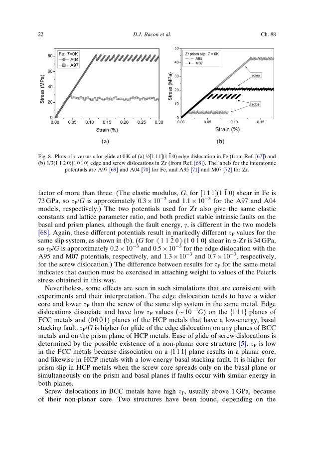
factor of more than three. (The elastic modulus, G, for [1 1 1]ð1 �1 0Þ shear in Fe is73 GPa, so tP/G is approximately 0.3� 10�3 and 1.1� 10�3 for the A97 and A04models, respectively.) The two potentials used for Zr also give the same elasticconstants and lattice parameter ratio, and both predict stable intrinsic faults on thebasal and prism planes, although the fault energy, g, is different in the two models[68]. Again, these different potentials result in markedly different tP values for thesame slip system, as shown in (b). (G for /1 1 �2 0Sf1 0 �1 0g shear in a-Zr is 34 GPa,so tP/G is approximately 0.2� 10�3 and 0.5� 10�3 for the edge dislocation with theA95 and M07 potentials, respectively, and 1.3� 10�3 and 0.7� 10�3, respectively,for the screw dislocation.) The difference between results for tP for the same metalindicates that caution must be exercised in attaching weight to values of the Peierlsstress obtained in this way.

Nevertheless, some effects are seen in such simulations that are consistent withexperiments and their interpretation. The edge dislocation tends to have a widercore and lower tP than the screw of the same slip system in the same metal. Edgedislocations dissociate and have low tP values (B10�4G) on the {1 1 1} planes ofFCC metals and (0 0 0 1) planes of the HCP metals that have a low-energy, basalstacking fault. tP/G is higher for glide of the edge dislocation on any planes of BCCmetals and on the prism plane of HCP metals. Ease of glide of screw dislocations isdetermined by the possible existence of a non-planar core structure [5]. tP is lowin the FCC metals because dissociation on a {1 1 1} plane results in a planar core,and likewise in HCP metals with a low-energy basal stacking fault. It is higher forprism slip in HCP metals when the screw core spreads only on the basal plane orsimultaneously on the prism and basal planes if faults occur with similar energy inboth planes.

Screw dislocations in BCC metals have high tP, usually above 1 GPa, becauseof their non-planar core. Two structures have been found, depending on the

Fig. 8. Plots of t versus e for glide at 0 K of (a) ½[1 1 1]ð1 �1 0Þ edge dislocation in Fe (from Ref. [67]) and(b) 1/3h1 1 �2 0if1 0 �1 0g edge and screw dislocations in Zr (from Ref. [68]). The labels for the interatomic

potentials are A97 [69] and A04 [70] for Fe, and A95 [71] and M07 [72] for Zr.


interatomic potential: a threefold degenerate core, proposed initially in Ref. [64]and predicted by early pair potentials (see Ref. [29]), and a non-degeneratecompact core, first observed in simplified MS simulations based on interactionpotentials between rows of atoms [73] and later predicted by ab initio calculations[38,63] and the interatomic potential in [70]. However, tP is somewhat ill-defined forthe BCC screw. With some potentials that predict a degenerate core [30,44], thedislocation advances by one atomic distance at a lower critical stress and adoptsa metastable sessile structure. It remains immobile until an upper critical stress isreached and motion then becomes unbounded. Also, tP is sensitive to non-Schmidcomponents in the applied stress, particularly normal stress perpendicular to theglide plane [44,74]. (See also Refs [5,6].)

3.1.2. Glide at finite temperatureThe minimum applied resolved shear stress for dislocation glide at TW0 K isless than tP because of thermal activation. When the stress is high enough sothat a dislocation no longer feels the Peierls stress, its free-flight motion hasa viscous character with steady-state velocity, vD, proportional to the resolved shearstress t

vD ¼tbB, (6)

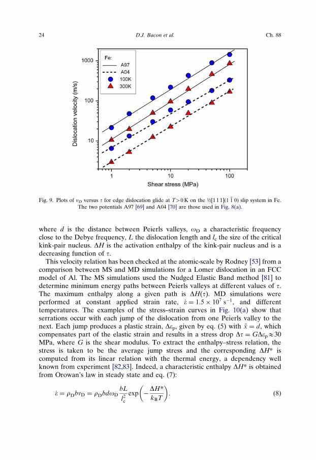
where B is a friction coefficient. With increasing stress, vD falls below values givenby eq. (6) and tends asymptotically to the transverse sound velocity of the material(Bfew kms�1). B has various origins in real materials [75], but in MD simulationsis controlled solely by phonon damping. MD simulations using PAD models todetermine vD as a function of t yield values of B in the range 1–100 mPas [52,76–78].Examples of data obtained by simulation for vD versus t at 100 and 300 K for theedge dislocation in the two models of Fe used for Fig. 8(a) are presented in Fig. 9.It is seen that the potential from Ref. [70], which gives the higher tP, also results inlower vD for the same value of t. With log–log scales, the plots are linear withgradient equal to 1, as expected from eq. (6), and the value of B increases withincreasing T due to increasing phonon damping. The relation between B and T wasshown to be linear in FCC metals and Fe [52,77], in agreement with Leibfried’stheory of phonon damping [75].

As proposed initially by Seeger [79], a dislocation in a high Peierls stresscrystal at TW0 K and low t spends most of its time aligned with the bottom ofa Peierls valley until thermally activated nucleation of a kink-pair moves partof it into the next valley. Subsequent propagation of the kinks along the linetransfers the rest of the dislocation to the new position. An early expressionbased on an analogy between a dislocation and a vibrating string was proposed byFriedel [80]:

vD ¼ doDb

lc

L

lcexp �

DHðtÞkBT

� �, (7)


where d is the distance between Peierls valleys, oD a characteristic frequencyclose to the Debye frequency, L the dislocation length and lc the size of the criticalkink-pair nucleus. DH is the activation enthalpy of the kink-pair nucleus and is adecreasing function of t.

This velocity relation has been checked at the atomic-scale by Rodney [53] from acomparison between MS and MD simulations for a Lomer dislocation in an FCCmodel of Al. The MS simulations used the Nudged Elastic Band method [81] todetermine minimum energy paths between Peierls valleys at different values of t.The maximum enthalpy along a given path is DH(t). MD simulations wereperformed at constant applied strain rate, _� ¼ 1:5� 107 s�1, and differenttemperatures. The examples of the stress–strain curves in Fig. 10(a) show thatserrations occur with each jump of the dislocation from one Peierls valley to thenext. Each jump produces a plastic strain, Dep, given by eq. (5) with �x ¼ d, whichcompensates part of the elastic strain and results in a stress drop Dt ¼ GDepE30MPa, where G is the shear modulus. To extract the enthalpy–stress relation, thestress is taken to be the average jump stress and the corresponding DH* iscomputed from its linear relation with the thermal energy, a dependency wellknown from experiment [82,83]. Indeed, a characteristic enthalpy DH* is obtainedfrom Orowan’s law in steady state and eq. (7):

_� ¼ rDbvD ¼ rDbdoDbL

l2cexp �

DH*kBT

� �. (8)

Fig. 9. Plots of vD versus t for edge dislocation glide at TW0 K on the ½[1 1 1]ð1 �1 0Þ slip system in Fe.The two potentials A97 [69] and A04 [70] are those used in Fig. 8(a).


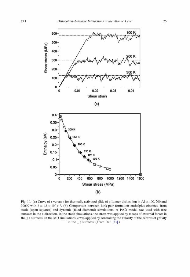
Fig. 10. (a) Curve of t versus e for thermally activated glide of a Lomer dislocation in Al at 100, 200 and300 K with _� ¼ 1:5� 107 s�1. (b) Comparison between kink-pair formation enthalpies obtained fromstatic (open squares) and dynamic (filled diamond) simulations. A PAD model was used with freesurfaces in the z direction. In the static simulations, the stress was applied by means of external forces inthe7z surfaces. In the MD simulations, _� was applied by controlling the velocity of the centres of gravity

in the7z surfaces. (From Ref. [53].)


Taking logarithms of both sides yields

DH* ¼ kBT lnrDbdoDbL

l2c _�

!. (9)

Setting oD ¼ 5� 1013 s�1, b ¼ d ¼ 0.258 nm, L ¼ 9.7 nm (¼Ly of the model),rD ¼ 10�2 nm�2 and lc ¼ b, gives DH* ¼ CkBT with C ¼ 11.3. This proportionalitycoefficient is significantly smaller than that in experiments (C ¼ 25B30) because ofthe high applied strain rate. Fig. 10(b) compares the enthalpy curve with the resultof the static simulations, proving the accuracy of the velocity law of eq. (8) for therange of T and _� explored here.

3.1.3. Comparison with experimentA striking difference between modelling and experiment is that the Peierls stresspredicted from atomic-scale simulations is several times larger than values deducedfrom experiment. For instance, with the Fe interatomic potentials used above,the Peierls stress for the ½/1 1 1S screw dislocation in Fe is above 1 GPa while theexperimental value is 400 MPa [84]. A similar observation has been made forpotassium [85]. High values have also been obtained with ab initio calculations [38],with the exception of molybdenum modelled within the Generalized Pseudopo-tential Theory [37]. Various explanations have been put forward to explain thediscrepancy, such as the effect of kink dynamics [38], stress concentrations [86] andcollective behaviour of dislocations [87]. More research is needed to provide betterunderstanding of this discrepancy.

3.2. Glide in solid solutions

3.2.1. BackgroundThe yield and flow stress of a metal can be strongly influenced by the presence ofsolute atoms, an effect that is exploited in ‘alloy strengthening’. Whether in solution(SSH) or in precipitates of a second phase (‘precipitation strengthening’), the soluteatoms make the metal inhomogeneous at the atomic scale and create a resistanceto dislocation glide, e.g. Refs [88,89]. Simulations of solid solutions are described inthis section and precipitates are considered in Section 4.

There are two principal issues involved in attempting to model SSH and gain aquantitative estimate of the critical applied stress for glide. One is concerned withthe short-range interaction of a dislocation with the solute obstacles, which wereturn to below. The other arises from the statistical nature of the distribution ofobstacles in an alloy. Foreman and Makin [90] made the first computer simulationstudy of this problem in the approximation of constant line tension to model glide ofa dislocation in a field of randomly positioned pinning points, and an analyticaltreatment was presented by Kocks [91]. More sophisticated approaches to thestatistical nature of SSH have also been considered in semi-analytical treatments,e.g. in Refs [92–95]. (A review of some of the earlier models has been presented byHaasen [96].) It is not possible to address this issue quantitatively by MD simulation


because the simulation cells required to obtain results with statistical significancewould be too large. Instead, atomic-scale modelling has mainly focused on the inter-action between a dislocation and one or a few solute atoms near or within its core.

Until recently, this interaction was derived from the long-range solution obtainedby linear elasticity theory. Solutes can be modelled using several descriptionsdepending on their nature [2–4]. The simplest considers each solute atom to bea centre of dilatation due to its misfit in the solvent crystal. As a result of theassociated volume change, a dislocation interacts with the solute if it has a non-zeropressure component in its stress field. The interaction energy decreases as (r)�1,where r is the distance from the solute atom to the dislocation core, and canbe negative (attractive) or positive (repulsive) depending on the position of thesolute atom with respect to the dislocation. If the symmetry of the site occupiedby the solute atom is lower than that of the perfect crystal, more than one distinctorientation of that atom must exist, i.e. its distortion field is not sphericallysymmetric: consequently there is an interaction with the shear stress field of adislocation, again proportional to (r)�1. Substitutional solute atoms in metallicalloys do not lower the symmetry: examples treated by atomic-scale simulationinclude Cu and Cr in Fe, Al in Ni and Mg in Al (see Section 3.2.2). Interstitialsolutes may lower the symmetry, the classic case being that of carbon (C) in Fe, forwhich the C atom occupies an octahedral site and creates a distortion withtetragonal rather than cubic symmetry (see Section 3.2.3). An induced interactioncan also arise if the elastic properties of the solute atom are different from the hostcrystal. This interaction is of order (r)�2.

These descriptions based on elasticity theory break down when r tends to zero,i.e. within the dislocation core, and atomic-scale simulations are adopted. Ab initiomethods can be used to model single solute atoms or small clusters in the core [97],but, due to their computational cost, cannot be used to simulate dislocationmotion in a solid solution. The PAD method and short-range potentials discussedin Section 2 are suitable. Although specific electronic effects of solute atoms cannotbe represented by these potentials, properties such as size misfit or symmetry-breaking can.

3.2.2. Substitutional solute atomsAlloys simulated to date include solutions of Al in Ni (FCC), Mg in Al (FCC) andCu or Cr in Fe (BCC). A significant source of hardening comes from the short-range interaction of the dislocation with particular configurations of solute atoms,specifically pairs of solute atoms across or along the dislocation glide plane, ratherthan more diffuse, long-range interaction as in classical SSH theories [96].

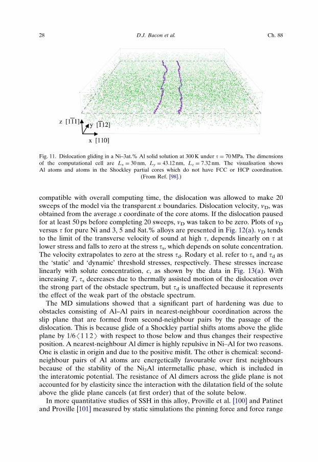
In the case of Al in Ni, nearest-neighbour pairs of Al atoms with one atom justbelow and one just above the dislocation glide plane are strong pinning centres.Rodary et al. [98] simulated the glide of an edge dislocation with PAD boundariesunder constant applied shear stress for solute concentration, c, in the range 1–8at.%. An example is shown in Fig. 11. With the interatomic potential set used, anAl atom is oversized with a volume misfit parameter of 3%. To ensure that thegliding dislocation encountered the most representative random arrangement


compatible with overall computing time, the dislocation was allowed to make 20sweeps of the model via the transparent x boundaries. Dislocation velocity, vD, wasobtained from the average x coordinate of the core atoms. If the dislocation pausedfor at least 50 ps before completing 20 sweeps, vD was taken to be zero. Plots of vD

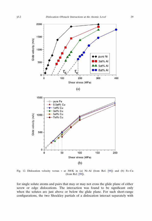
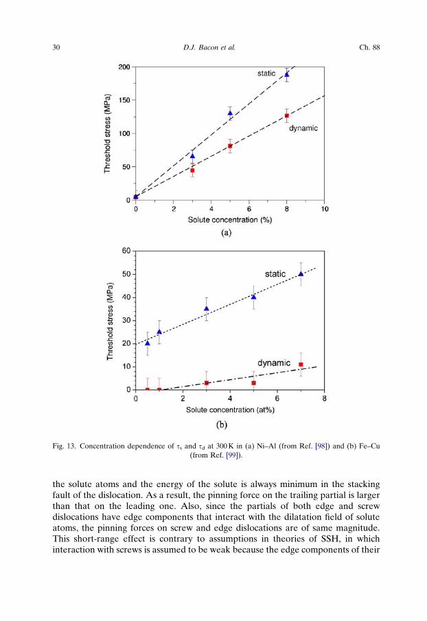
versus t for pure Ni and 3, 5 and 8at.% alloys are presented in Fig. 12(a). vD tendsto the limit of the transverse velocity of sound at high t, depends linearly on t atlower stress and falls to zero at the stress ts, which depends on solute concentration.The velocity extrapolates to zero at the stress td. Rodary et al. refer to ts and td asthe ‘static’ and ‘dynamic’ threshold stresses, respectively. These stresses increaselinearly with solute concentration, c, as shown by the data in Fig. 13(a). Withincreasing T, ts decreases due to thermally assisted motion of the dislocation overthe strong part of the obstacle spectrum, but td is unaffected because it representsthe effect of the weak part of the obstacle spectrum.

The MD simulations showed that a significant part of hardening was due toobstacles consisting of Al–Al pairs in nearest-neighbour coordination across theslip plane that are formed from second-neighbour pairs by the passage of thedislocation. This is because glide of a Shockley partial shifts atoms above the glideplane by 1/6/1 1 2S with respect to those below and thus changes their respectiveposition. A nearest-neighbour Al dimer is highly repulsive in Ni–Al for two reasons.One is elastic in origin and due to the positive misfit. The other is chemical: second-neighbour pairs of Al atoms are energetically favourable over first neighboursbecause of the stability of the Ni3Al intermetallic phase, which is included inthe interatomic potential. The resistance of Al dimers across the glide plane is notaccounted for by elasticity since the interaction with the dilatation field of the soluteabove the glide plane cancels (at first order) that of the solute below.

In more quantitative studies of SSH in this alloy, Proville et al. [100] and Patinetand Proville [101] measured by static simulations the pinning force and force range

Fig. 11. Dislocation gliding in a Ni–3at.% Al solid solution at 300 K under t ¼ 70 MPa. The dimensionsof the computational cell are Lx ¼ 30 nm, Ly ¼ 43.12 nm, Lz ¼ 7.32 nm. The visualisation showsAl atoms and atoms in the Shockley partial cores which do not have FCC or HCP coordination.

(From Ref. [98].)


for single solute atoms and pairs that may or may not cross the glide plane of eitherscrew or edge dislocations. The interaction was found to be significant onlywhen the solutes are just above or below the glide plane. For such short-rangeconfigurations, the two Shockley partials of a dislocation interact separately with

Fig. 12. Dislocation velocity versus t at 300 K in (a) Ni–Al (from Ref. [98]) and (b) Fe–Cu(from Ref. [99]).


the solute atoms and the energy of the solute is always minimum in the stackingfault of the dislocation. As a result, the pinning force on the trailing partial is largerthan that on the leading one. Also, since the partials of both edge and screwdislocations have edge components that interact with the dilatation field of soluteatoms, the pinning forces on screw and edge dislocations are of same magnitude.This short-range effect is contrary to assumptions in theories of SSH, in whichinteraction with screws is assumed to be weak because the edge components of their

Fig. 13. Concentration dependence of ts and td at 300 K in (a) Ni–Al (from Ref. [98]) and (b) Fe–Cu(from Ref. [99]).


partials have opposite sign and cancel at large distance. The CRSS at T ¼ 0 K forboth edge and screw dislocations increases linearly with c at the same rate, about25–30 MPa/at.%, in agreement with experimental indentation hardness measure-ments on Ni–Al [102]. The strongest configuration for both edge and screwdislocations is a dimer of solute atoms in the plane just above the glide plane: thepinning force is about twice that for a solute atom in the same plane, which is thelocation for a single atom with the highest obstacle strength. The second strongestconfiguration is the dimer that crosses the glide plane, as described above. Pinningforces found by simulation are smaller than estimates obtained by elasticity theory,showing that the latter does not account accurately for the short-range interactions.

The interaction energy of edge and screw dislocations with single solute atoms inthe Al–Mg system was computed using cylindrical simulation cells with RBCs andno loading in Ref. [103]. The interaction energy with the two partials is symmetricalin this case because the dislocation is at rest. As in Ni–Al, the strongest interactionis when the solute atom is in a plane adjacent to the glide plane.

The importance of short-range interactions has also been confirmed for the BCCalloy Fe–Cu, in which Cu is an oversized substitutional solute. MS simulation ofmotion of the ½/1 1 1Sf1 �1 0g edge dislocation under increasing strain shows thatthe critical stress, tc, is determined by individual obstacles in the form of eithersingle Cu atoms or pairs of solute atoms adjacent to the glide plane [99]. For singleatoms, tc is highest when the solute occupies a site in the plane immediately belowthe extra half-plane of the dislocation. It is the one that gives the maximumattractive interaction energy with the dislocation. For Cu–Cu doublets, themaximum tc is approximately 50% higher than that for one solute atom andoccurs for the first-neighbour pair in the plane immediately below the extra half-plane. This configuration is equivalent to the strongest obstacle pair in Ni–Al,except that in that case the pair is above the glide plane. By varying the model sizein the simulations of individual obstacles, tc was found to be approximatelyproportional to the reciprocal of the spacing of strong obstacles along thedislocation line, a result consistent with the continuum treatment of localised-obstacle strengthening.

MD simulation of edge dislocation glide in Fe–Cu solid solutions at TW0 Krevealed similar behaviour to that in Ni–Al discussed above, i.e. smooth motionwith constant velocity at high t and irregular motion with pauses and completestops at low t [99]. Plots for vD versus t in Fe–Cu solutions at 300 K are shown inFig. 12(b). They have similar form to those for Ni–Al in (a), but vD at a given stressis much less sensitive to change in c. The threshold stresses ts and td defined inFig. 12(a) are plotted as functions of c for Fe–Cu in Fig. 13(b). Both increaselinearly with c, but, unlike those for Ni–Al, do not extrapolate to the same value atc ¼ 0. Tapasa et al. note that dislocation glide in the equivalent simulation of pureFe occurs at tB1 MPa, so even a concentration as small as 0.5at.% of Cu in Fe has asignificant effect on ts.

Rodary et al. [98] have pointed out that the linear dependence of ts on c isconsistent with the importance of the strongest obstacles in the solute spectrum,because, according to Friedel statistics [80], the stress at which a dislocation moves


across a field of point obstacles is proportional to the square root of obstacledensity, and the density of pairs of solute atoms is proportional to solute concentra-tion. It is also consistent with interpretation of the experimental concentration-dependence of hardening in Cu–Mn solid solutions, according to which pairs of Mnatoms are responsible for the hardening [104].

3.2.3. Interstitial solute atomsThe important role of carbon interstitial solute in the phenomena of yielding andstrain ageing in steel was first treated theoretically via elasticity in [105]. Thesignificance of the interaction of carbon atoms with the dislocation core itself wasidentified, but it has been possible only recently to examine this within the scope oflarge-scale atomic simulations. Potentials that accurately reproduce all importantproperties of C in Fe have not been available, so Tapasa et al. [106] employed acombination of the EAM interatomic potential for Fe–Fe interaction from Ref. [69]and a pair potential for Fe–C interaction from Ref. [107], which models an atomhaving the same octahedral site and distortion field as C in Fe and similar migrationenergy. Carbon in this low symmetry site creates a tetragonal distortion, for it repelsits two first-neighbour Fe atoms in a /1 0 0S direction and attracts its four secondneighbours in the two transverse /0 1 1S directions. Thus, C solutes are located ineither a ð1 �1 0Þ atomic plane parallel to the dislocation glide plane (with tetragonaldistortion axis (TDA) in the [0 0 1] direction) or sites between two ð1 �1 0Þ planes(with [1 0 0] or [0 1 0] TDAs symmetric about b).

Tapasa et al. [106] used MS to investigate the interaction energy of the edgedislocation with a C atom in sites near the slip plane. Sites half an interplanarspacing below the ð1 �1 0Þ plane at the bottom of the extra half-plane have thehighest binding energy, Eb ¼ 0.68 eV. C atoms in sites within ð1 �1 0Þ atomic planeshave a maximum Eb of 0.5 eV when located one below the extra half-plane. Thesevalues compare with the elasticity estimate of about 0.5 eV obtained in Ref. [105]and values in the range 0.5–0.8 eV calculated later when the influence of thetetrahedral distortion was taken into account, e.g. Refs [108–111]. This distortiongives rise to C interaction with the ½/1 1 1S screw dislocation, for which Eb ispredicted to be approximately 40% of the value for the edge [111]. Interestingly,Becquart et al. [112] have recently developed a new potential for a C atom in Feusing ab initio data and find that the maximum Eb for the screw dislocation is0.41 eV. Thus, although maximum binding occurs inside the core region wherelinear elasticity is not strictly valid, the Eb value it gives for C in Fe is consistent withthe atomic-level treatments.

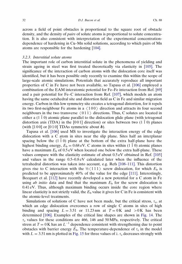
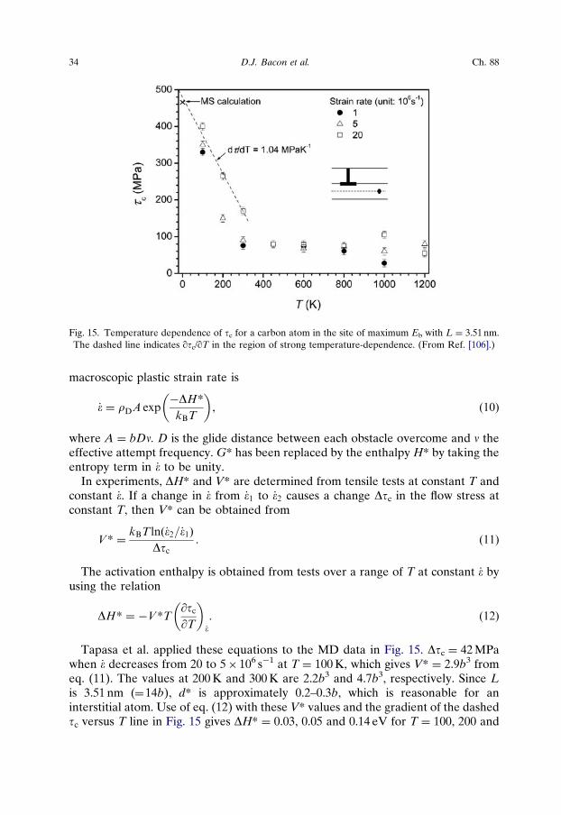
Simulations of solutions of C have not been made, but the critical stress, tc, atwhich an edge dislocation overcomes a row of single C atoms in sites of highbinding and spacing L ¼ 3.51 or 11.23 nm at T ¼ 0 K and W0 K has beendetermined [106]. Examples of the critical line shapes are shown in Fig. 14. Thetc values for these conditions are 466, 146 and 50 MPa, respectively. The criticalstress at T ¼ 0 K has an L�1 dependence consistent with strengthening due to pointobstacles with barrier energy Eb. The temperature-dependence of tc in the modelwith L ¼ 3.51 nm is plotted in Fig. 15 for three values of _�. tc decreases strongly with


increasing T at low T and increases with increasing _�. It is small and largelyindependent of T above about 300 K. Carbon atom migration within the core occursduring the time the dislocation is pinned when TZ800 K, but extensive drag ofsolute does not occur at the applied strain rates accessible to MD simulationbecause the dislocation jumps forward by too large a distance as it unpins for aC atom to be recaptured.

Tapasa et al. deduced the activation parameters for slip in this atomic-scalemodel with the following treatment. Dislocations slip by overcoming barriers, eachof which exerts a resisting force with a profile such that the area under the force–distance curve equals the total energy, Eb. (See, e.g. Refs [2,113,114].) At TW0 K,the energy required is partly provided as mechanical work by the applied load: it iswritten tcbLd* or tcV*, where d* and V* are the activation distance and volume,respectively. The remainder is thermal and has to overcome the free energy ofactivation DG* ¼ Eb*� tcV*, where Eb* is the total energy required between thedislocation states separated by d*. DG* is the Gibbs free energy change at constantT and _� between those two states. The probability of DG* being provided bythermal fluctuations is exp(�DG*/kBT) if DG*ckBT. Hence, from eq. (8) the

Fig. 14. Edge dislocation shape (visualised by atoms in the core) at tc for a carbon atom (small sphere) inthe site of maximum binding energy, Eb, in Fe crystals at (a, b) T ¼ 0 K for two different spacings, L,between carbon atoms and (c) T ¼ 300 K. The applied strain rate is _� ¼ 5� 106 s�1. (From Ref. [106].)


macroscopic plastic strain rate is

_� ¼ rDA exp�DH*kBT

� �, (10)

where A ¼ bDn. D is the glide distance between each obstacle overcome and n theeffective attempt frequency. G* has been replaced by the enthalpy H* by taking theentropy term in _� to be unity.

In experiments, DH* and V* are determined from tensile tests at constant T andconstant _�. If a change in _� from _�1 to _�2 causes a change Dtc in the flow stress atconstant T, then V* can be obtained from

V* ¼kBT lnð_�2=_�1Þ

Dtc. (11)

The activation enthalpy is obtained from tests over a range of T at constant _� byusing the relation

DH* ¼ �V*T@tc@T

� �_�

. (12)

Tapasa et al. applied these equations to the MD data in Fig. 15. Dtc ¼ 42 MPawhen _� decreases from 20 to 5� 106 s�1 at T ¼ 100 K, which gives V* ¼ 2.9b3 fromeq. (11). The values at 200 K and 300 K are 2.2b3 and 4.7b3, respectively. Since Lis 3.51 nm (¼14b), d* is approximately 0.2–0.3b, which is reasonable for aninterstitial atom. Use of eq. (12) with these V* values and the gradient of the dashedtc versus T line in Fig. 15 gives DH* ¼ 0.03, 0.05 and 0.14 eV for T ¼ 100, 200 and

Fig. 15. Temperature dependence of tc for a carbon atom in the site of maximum Eb with L ¼ 3.51 nm.The dashed line indicates qtc/qT in the region of strong temperature-dependence. (From Ref. [106].)


300 K, respectively, i.e. 3–6kBT. This energy is much smaller than Eb ¼ 0.68 eV thathas to be overcome by the dislocation at T ¼ 0 K. This exposes a limitation of MDfor simulation of thermally activated dislocation processes already mentionedin Section 2.5. The unavoidably high _� limits the time available for activationand results in small values of DH*, as mentioned at the end of Section 3.1.2. Thisconclusion was also drawn by Domain and Monnet [43], who used MD simulationof glide of a ½/1 1 1S screw dislocation in Fe to reveal that DH* is B20kBT smallerthan that realised in experiment at much smaller strain rate.

3.2.4. Extension to microscopic modelsAn outstanding issue in relation to MD simulation of SSH is how to incorporateinformation gained from relatively small models into larger-scale analyses thatrecognise the statistical nature of dislocation behaviour. Rodary et al. [98] haveprovided a brief discussion of how results from their MD modelling of Ni–Al mightbe incorporated in a higher-level, micromechanical approach to predict macro-scopic stress–strain curves. Proville et al. [100,101] used the pinning forces and forceranges computed from MS simulations to parameterise analytical expressions ofCRSS proposed in various classical theories of SSH [96]. One difficulty is that thetheories assume a single type of obstacle whereas simulations exhibit a range ofpinning forces depending on obstacle type (single atom or dimer) and position withrespect to the glide plane. A generalisation of the Mott–Nabarro model to includeseveral types of obstacles was proposed in Ref. [100] and showed good agreementwith MS simulations. Olmsted et al. [103] proposed a semi-analytical approachbased on computation of a one-dimensional energy landscape for the motion of astraight edge dislocation through a random field of Mg solutes in Al using the singlesolute energy values. The stress to unpin a straight edge dislocation trapped ina local energy minimum was estimated and compared with values obtained by MSfor a dislocation moving under stress through a random array of solutes. A goodagreement was obtained. The thermally activated rate of dislocation unpinningversus t and T was calculated semi-analytically, and again good agreement wasfound with results of MD simulations.

A challenge for future work in this area is to provide more accurate informationon the motion of dislocation cores containing solute atoms across wide ranges ofT and vD, and build it into continuum-based models so that effects such asdislocation–dislocation interactions and dislocation climb can be simulated.

4. Voids and precipitates

4.1. Introduction

We now turn to obstacles that are larger than the individual solute atomsconsidered in Section 3, but are still only up to a few nanometres in size. As noted inSection 1, much of the research using atomic-scale simulation has been driven bythe need to investigate the effect of obstacles that are of importance for metals in


current and future nuclear power systems. MD simulation of displacement cascadesshows that a significant fraction of the point defects are created in clusters with theirown kind. SIA clusters are usually in the form of dislocation loops. The clusteredvacancies resulting from radiation damage may have dislocation character, i.e.loops or SFTs. These vacancy clusters also form during annealing of the vacancysupersaturation created by rapid quenching of metals from temperatures just belowthe melting point. The obstacle properties of dislocation loops and SFTs areconsidered in Section 5.

In many situations, vacancies cluster to form voids. Voids are common featuresof the microstructure after either irradiation at high temperature or ageing afterquenching. When He atoms are present, e.g. as a result of a transmutation reactionwith atoms in the metal, these cavities may contain He gas. Voids are usually ofnear-spherical shape, with facets on close-packed planes that have low surfaceenergy. It will be seen below that they can offer strong resistance to dislocationmotion as a result of direct contact between dislocation and void. The interactionis characterised by the following. It is energetically favourable for a dislocation tointersect a void because its core and strain energy is zero within the cavity.However, this is at least partially offset by the fact that the dislocation has to createa surface step (in the direction of b) by shear as it penetrates a void. These twoeffects determine the obstacle strength of the void, i.e. the magnitude of the appliedstress that is necessary for the dislocation to break away. These important details,and the effect of the cavity on the dislocation energy, are not easily modelled usingelasticity theory [115].

Precipitates also form a class of obstacle known to be important for the strengthof alloys, e.g. Refs [88,89]. For many applications, alloy composition and heattreatment are deliberately chosen to develop a population of precipitates thatoffers optimum resistance to dislocation motion and is stable in the temperaturerange required for use. In terms of atomic-scale simulation, such alloys havereceived little attention because the size and dispersion of their precipitates are suchthat the strengthening mechanisms are quite well understood from conventional,continuum-based models. Computer simulation has tended to focus on alloysystems where the precipitates are small and research is required to understand thedislocation–precipitate mechanisms at the atomic level. The alloys in question areagain important for current and future nuclear power systems. They are Fe–Cu andFe–Cr, and are also considered in this section.

If the dislocation penetrates and shears a precipitate, the features that determinethe obstacle strength may be similar to those mentioned for a void, i.e. an interfacestep has to be created and the dislocation energy in the precipitate may be differentfrom that in the surrounding matrix, in this case as a result of differences in propertiessuch as the elastic constants and stacking fault energy. Furthermore, the dislocationmay induce a change within the precipitate to a more favourable crystal structure, aneffect discovered by computer simulation of Cu precipitates in Fe (see below). Thefeatures of strengthening are different, however, if the dislocation does not penetratethe precipitate, e.g. if the precipitate is incoherent with the matrix or if the stress statenear it is sufficient to induce the dislocation to bypass it by cross-slip.


Important details that determine the critical applied stress and breakawaymechanism are not easily modelled using elasticity theory. For example, the surfacestep on a void (or interface step around a precipitate) increases in size to b asan edge dislocation is pulled from the obstacle, in contrast to the situation for ascrew where it decreases to zero, and the energy of the step may not be known withprecision. Furthermore, the effect of a small void or precipitate on the dislocationenergy and stress field can only be treated with approximation. Atomic-levelsimulation incorporates these effects naturally. We first consider the obstacleresistance encountered by edge dislocations due voids in Fe and Cu (Section 4.2.1)and precipitates in Fe (Section 4.2.2) at T ¼ 0 K. In this MS modelling, shear strain eis applied in increments De and the potential energy, E, is minimised after everyincrement: the applied shear stress,t, is calculated from the reaction force exertedby the moveable atoms on the rigid outer blocks of atoms (Section 2.5). MSsimulation neglects effects due to kinetic energy and provides for direct comparisonwith continuum modelling of these obstacles (Section 4.2.3). The effects oftemperature on void and precipitate strengthening are presented in Section 4.3, andexamples of simulations of bubbles and loose clusters of vacancies are described inSection 4.4.

4.2. Edge dislocation–obstacle interaction at T ¼ 0 K

4.2.1. VoidsThis interaction has been most widely studied for Fe using the interatomic potentialfrom Ref. [69]. The computational cell and BCC crystallographic indices for theedge dislocation are shown schematically in Fig. 16(a). A spherical void of diameterD is placed with its equator on the dislocation slip plane. The periodic spacing ofvoids in the y direction is L. (From now on, we use L for the obstacle spacing ofboth edge and screw dislocations, i.e. for Ly and Lx respectively.) Results for 339-vacancy voids (D ¼ 2 nm) in a crystal of 2.07 M atoms (L ¼ 41.4 nm, Lx ¼ 29.8 nm,Lz ¼ 19.9 nm) are presented in Fig. 17(a) as curves of t and DE versus e, where DEis the change in E from the initial state when the straight dislocation is far from therow of voids. Four regions are indicated on the plots. The dislocation glides towardsthe void at the Peierls stress of 23 MPa in region I. It is attracted by, and pulled into,the void in region II: a step of length b is created on the entry surface of the void butE decreases because of the decrease in length of the dislocation. Stress becomesnegative because the plastic shear strain due to dislocation motion is larger than theimposed strain: t does not return to zero until e increases and the dislocationbecomes straight and coincident with the centre-to-centre line of the voids, i.e. theminimum energy configuration is achieved. In region III the dislocation bowsbetween the voids under increasing e until it is released at the critical resolved shearstress, tc. As shown in Fig. 7, visualisation of the atoms in the dislocation coredemonstrates that on breaking away, the dislocation absorbs a few vacancies from avoid and so acquires a pair of superjogs, i.e. jogs of more than one-atom height.Region IV corresponds to motion of the jogged dislocation. The dependence of the


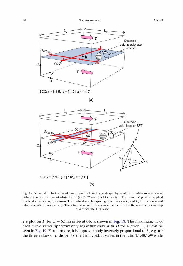
t–e plot on D for L ¼ 62 nm in Fe at 0 K is shown in Fig. 18. The maximum, tc, ofeach curve varies approximately logarithmically with D for a given L, as can beseen in Fig. 19. Furthermore, it is approximately inversely proportional to L, e.g. forthe three values of L shown for the 2 nm void, tc varies in the ratio 1:1.40:1.99 while

Fig. 16. Schematic illustration of the atomic cell and crystallography used to simulate interaction ofdislocations with a row of obstacles in (a) BCC and (b) FCC metals. The sense of positive appliedresolved shear stress, t, is shown. The centre-to-centre spacing of obstacles is Lx and Ly for the screw andedge dislocations, respectively. The tetrahedron in (b) is also used to identify the Burgers vectors and slip

planes for the FCC case.


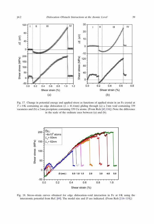
Fig. 17. Change in potential energy and applied stress as functions of applied strain in an Fe crystal atT ¼ 0 K containing an edge dislocation (L ¼ 41.4 nm) gliding through (a) a 2 nm void containing 339vacancies and (b) a 2 nm precipitate containing 339 Cu atoms. (From Refs [42,116].) Note the difference

in the scale of the ordinate axes between (a) and (b).

Fig. 18. Stress–strain curves obtained for edge dislocation–void interaction in Fe at 0 K using theinteratomic potential from Ref. [69]. The model size and D are indicated. (From Refs [116–119].)


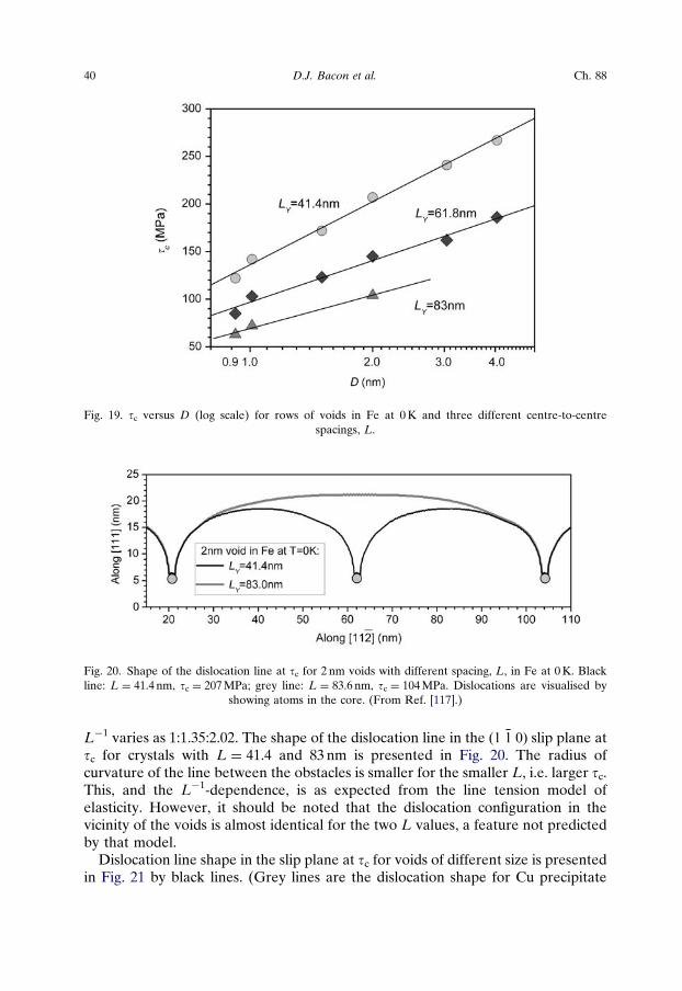
L�1 varies as 1:1.35:2.02. The shape of the dislocation line in the ð1 �1 0Þ slip plane attc for crystals with L ¼ 41.4 and 83 nm is presented in Fig. 20. The radius ofcurvature of the line between the obstacles is smaller for the smaller L, i.e. larger tc.This, and the L�1-dependence, is as expected from the line tension model ofelasticity. However, it should be noted that the dislocation configuration in thevicinity of the voids is almost identical for the two L values, a feature not predictedby that model.

Dislocation line shape in the slip plane at tc for voids of different size is presentedin Fig. 21 by black lines. (Grey lines are the dislocation shape for Cu precipitate

Fig. 19. tc versus D (log scale) for rows of voids in Fe at 0 K and three different centre-to-centrespacings, L.

Fig. 20. Shape of the dislocation line at tc for 2 nm voids with different spacing, L, in Fe at 0 K. Blackline: L ¼ 41.4 nm, tc ¼ 207 MPa; grey line: L ¼ 83.6 nm, tc ¼ 104 MPa. Dislocations are visualised by

showing atoms in the core. (From Ref. [117].)


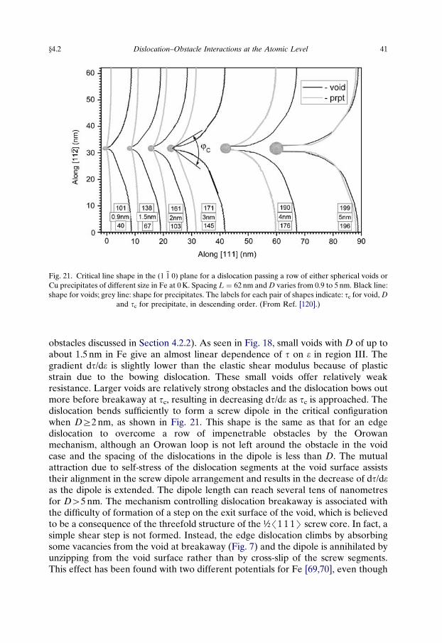
obstacles discussed in Section 4.2.2). As seen in Fig. 18, small voids with D of up toabout 1.5 nm in Fe give an almost linear dependence of t on e in region III. Thegradient dt/de is slightly lower than the elastic shear modulus because of plasticstrain due to the bowing dislocation. These small voids offer relatively weakresistance. Larger voids are relatively strong obstacles and the dislocation bows outmore before breakaway at tc, resulting in decreasing dt/de as tc is approached. Thedislocation bends sufficiently to form a screw dipole in the critical configurationwhen DZ2 nm, as shown in Fig. 21. This shape is the same as that for an edgedislocation to overcome a row of impenetrable obstacles by the Orowanmechanism, although an Orowan loop is not left around the obstacle in the voidcase and the spacing of the dislocations in the dipole is less than D. The mutualattraction due to self-stress of the dislocation segments at the void surface assiststheir alignment in the screw dipole arrangement and results in the decrease of dt/deas the dipole is extended. The dipole length can reach several tens of nanometresfor DW5 nm. The mechanism controlling dislocation breakaway is associated withthe difficulty of formation of a step on the exit surface of the void, which is believedto be a consequence of the threefold structure of the ½/1 1 1S screw core. In fact, asimple shear step is not formed. Instead, the edge dislocation climbs by absorbingsome vacancies from the void at breakaway (Fig. 7) and the dipole is annihilated byunzipping from the void surface rather than by cross-slip of the screw segments.This effect has been found with two different potentials for Fe [69,70], even though

Fig. 21. Critical line shape in the ð1 �1 0Þ plane for a dislocation passing a row of either spherical voids orCu precipitates of different size in Fe at 0 K. Spacing L ¼ 62 nm and D varies from 0.9 to 5 nm. Black line:shape for voids; grey line: shape for precipitates. The labels for each pair of shapes indicate: tc for void, D

and tc for precipitate, in descending order. (From Ref. [120].)


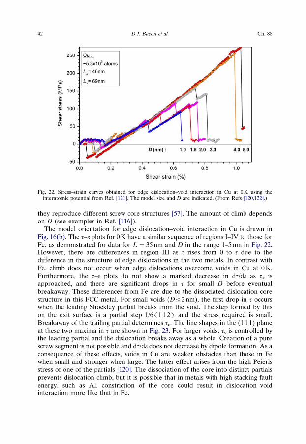
they reproduce different screw core structures [57]. The amount of climb dependson D (see examples in Ref. [116]).

The model orientation for edge dislocation–void interaction in Cu is drawn inFig. 16(b). The t–e plots for 0 K have a similar sequence of regions I–IV to those forFe, as demonstrated for data for L ¼ 35 nm and D in the range 1–5 nm in Fig. 22.However, there are differences in region III as t rises from 0 to t due to thedifference in the structure of edge dislocations in the two metals. In contrast withFe, climb does not occur when edge dislocations overcome voids in Cu at 0 K.Furthermore, the t–e plots do not show a marked decrease in dt/de as tc isapproached, and there are significant drops in t for small D before eventualbreakaway. These differences from Fe are due to the dissociated dislocation corestructure in this FCC metal. For small voids (Dr2 nm), the first drop in t occurswhen the leading Shockley partial breaks from the void. The step formed by thison the exit surface is a partial step 1/6/1 1 2S and the stress required is small.Breakaway of the trailing partial determines tc. The line shapes in the (1 1 1) planeat these two maxima in t are shown in Fig. 23. For larger voids, tc is controlled bythe leading partial and the dislocation breaks away as a whole. Creation of a purescrew segment is not possible and dt/de does not decrease by dipole formation. As aconsequence of these effects, voids in Cu are weaker obstacles than those in Fewhen small and stronger when large. The latter effect arises from the high Peierlsstress of one of the partials [120]. The dissociation of the core into distinct partialsprevents dislocation climb, but it is possible that in metals with high stacking faultenergy, such as Al, constriction of the core could result in dislocation–voidinteraction more like that in Fe.

Fig. 22. Stress–strain curves obtained for edge dislocation–void interaction in Cu at 0 K using theinteratomic potential from Ref. [121]. The model size and D are indicated. (From Refs [120,122].)


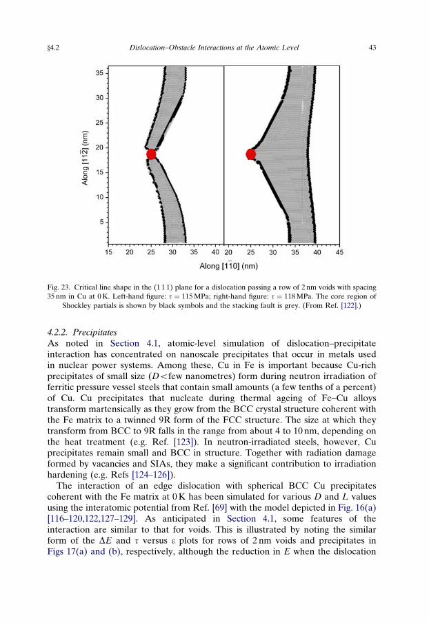
4.2.2. PrecipitatesAs noted in Section 4.1, atomic-level simulation of dislocation–precipitateinteraction has concentrated on nanoscale precipitates that occur in metals usedin nuclear power systems. Among these, Cu in Fe is important because Cu-richprecipitates of small size (Dofew nanometres) form during neutron irradiation offerritic pressure vessel steels that contain small amounts (a few tenths of a percent)of Cu. Cu precipitates that nucleate during thermal ageing of Fe–Cu alloystransform martensically as they grow from the BCC crystal structure coherent withthe Fe matrix to a twinned 9R form of the FCC structure. The size at which theytransform from BCC to 9R falls in the range from about 4 to 10 nm, depending onthe heat treatment (e.g. Ref. [123]). In neutron-irradiated steels, however, Cuprecipitates remain small and BCC in structure. Together with radiation damageformed by vacancies and SIAs, they make a significant contribution to irradiationhardening (e.g. Refs [124–126]).

The interaction of an edge dislocation with spherical BCC Cu precipitatescoherent with the Fe matrix at 0 K has been simulated for various D and L valuesusing the interatomic potential from Ref. [69] with the model depicted in Fig. 16(a)[116–120,122,127–129]. As anticipated in Section 4.1, some features of theinteraction are similar to that for voids. This is illustrated by noting the similarform of the DE and t versus e plots for rows of 2 nm voids and precipitates inFigs 17(a) and (b), respectively, although the reduction in E when the dislocation

Fig. 23. Critical line shape in the (1 1 1) plane for a dislocation passing a row of 2 nm voids with spacing35 nm in Cu at 0 K. Left-hand figure: t ¼ 115 MPa; right-hand figure: t ¼ 118 MPa. The core region of

Shockley partials is shown by black symbols and the stacking fault is grey. (From Ref. [122].)


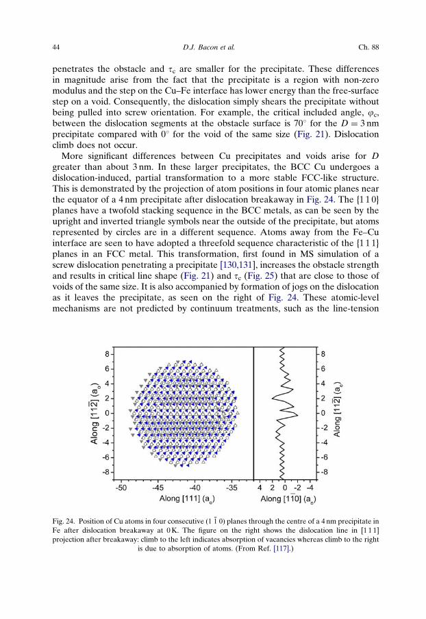
penetrates the obstacle and tc are smaller for the precipitate. These differencesin magnitude arise from the fact that the precipitate is a region with non-zeromodulus and the step on the Cu–Fe interface has lower energy than the free-surfacestep on a void. Consequently, the dislocation simply shears the precipitate withoutbeing pulled into screw orientation. For example, the critical included angle, jc,between the dislocation segments at the obstacle surface is 701 for the D ¼ 3 nmprecipitate compared with 01 for the void of the same size (Fig. 21). Dislocationclimb does not occur.

More significant differences between Cu precipitates and voids arise for Dgreater than about 3 nm. In these larger precipitates, the BCC Cu undergoes adislocation-induced, partial transformation to a more stable FCC-like structure.This is demonstrated by the projection of atom positions in four atomic planes nearthe equator of a 4 nm precipitate after dislocation breakaway in Fig. 24. The {1 1 0}planes have a twofold stacking sequence in the BCC metals, as can be seen by theupright and inverted triangle symbols near the outside of the precipitate, but atomsrepresented by circles are in a different sequence. Atoms away from the Fe–Cuinterface are seen to have adopted a threefold sequence characteristic of the {1 1 1}planes in an FCC metal. This transformation, first found in MS simulation of ascrew dislocation penetrating a precipitate [130,131], increases the obstacle strengthand results in critical line shape (Fig. 21) and tc (Fig. 25) that are close to those ofvoids of the same size. It is also accompanied by formation of jogs on the dislocationas it leaves the precipitate, as seen on the right of Fig. 24. These atomic-levelmechanisms are not predicted by continuum treatments, such as the line-tension

Fig. 24. Position of Cu atoms in four consecutive ð1 �1 0Þ planes through the centre of a 4 nm precipitate inFe after dislocation breakaway at 0 K. The figure on the right shows the dislocation line in [1 1 1]projection after breakaway: climb to the left indicates absorption of vacancies whereas climb to the right

is due to absorption of atoms. (From Ref. [117].)


and modulus-difference approximations that form the basis of the Russell–Brownmodel of Cu precipitate strengthening of Fe [132].

4.2.3. Comparison of atomistic and continuum results at 0 KThe simulations of the preceding section neglect kinetic effects and are the atomic-level equivalent of conventional linear elasticity modelling of dislocations. In thelatter, the simplest approach to strengthening due to a dispersion of localisedobstacles uses the line tension approximation. For a row of obstacles of spacing L,the dislocation breaks away when the forward force tbL on length L overcomesthe resistance of one obstacle, i.e. when the obstacle can no longer withstand theline tension force 2Gcos(j/2) imposed by the two segments of the bowing line at theobstacle: here G is the line tension (equal to approximately Gb2/2 in the constantline tension approximation) and j is the included angle between the segments,as shown for a 3 nm precipitate in Fig. 21. The critical stress is reached when j isreduced to the critical angle jc and so

tc ¼ aGb

L, (13)

where a ¼ cos(jc/2). A factor of approximately 0.8 has to be introduced to accountfor randomness in the obstacle arrangement [90,91]. It was seen in the data forvoids above that the dependence of tc on L�1 holds for atomic-scale interactions, asit should since there is no reason to doubt the Peach–Koehler expression that the

Fig. 25. Stress–strain curves obtained for interaction between an edge dislocation and Cu precipitateswith diameter D and spacing L ¼ 42 nm in Fe at 0 K. The model size and D are indicated.


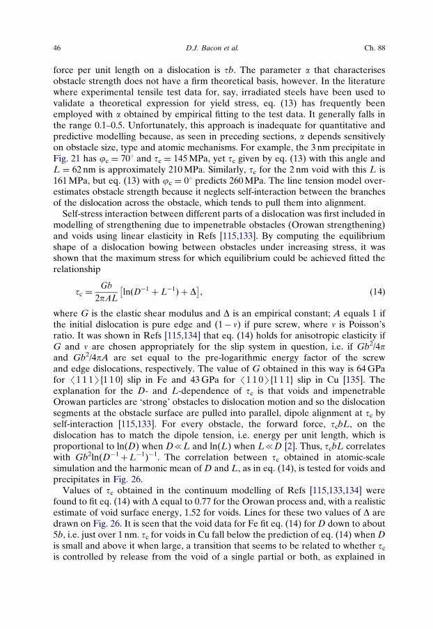
force per unit length on a dislocation is tb. The parameter a that characterisesobstacle strength does not have a firm theoretical basis, however. In the literaturewhere experimental tensile test data for, say, irradiated steels have been used tovalidate a theoretical expression for yield stress, eq. (13) has frequently beenemployed with a obtained by empirical fitting to the test data. It generally falls inthe range 0.1–0.5. Unfortunately, this approach is inadequate for quantitative andpredictive modelling because, as seen in preceding sections, a depends sensitivelyon obstacle size, type and atomic mechanisms. For example, the 3 nm precipitate inFig. 21 has jc ¼ 701 and tc ¼ 145 MPa, yet tc given by eq. (13) with this angle andL ¼ 62 nm is approximately 210 MPa. Similarly, tc for the 2 nm void with this L is161 MPa, but eq. (13) with jc ¼ 01 predicts 260 MPa. The line tension model over-estimates obstacle strength because it neglects self-interaction between the branchesof the dislocation across the obstacle, which tends to pull them into alignment.

Self-stress interaction between different parts of a dislocation was first included inmodelling of strengthening due to impenetrable obstacles (Orowan strengthening)and voids using linear elasticity in Refs [115,133]. By computing the equilibriumshape of a dislocation bowing between obstacles under increasing stress, it wasshown that the maximum stress for which equilibrium could be achieved fitted therelationship

tc ¼Gb

2pALlnðD�1 þ L�1Þ þ D� �

, (14)

where G is the elastic shear modulus and D is an empirical constant; A equals 1 ifthe initial dislocation is pure edge and (1� n) if pure screw, where n is Poisson’sratio. It was shown in Refs [115,134] that eq. (14) holds for anisotropic elasticity ifG and n are chosen appropriately for the slip system in question, i.e. if Gb2/4pand Gb2/4pA are set equal to the pre-logarithmic energy factor of the screwand edge dislocations, respectively. The value of G obtained in this way is 64 GPafor /1 1 1S{1 1 0} slip in Fe and 43 GPa for /1 1 0S{1 1 1} slip in Cu [135]. Theexplanation for the D- and L-dependence of tc is that voids and impenetrableOrowan particles are ‘strong’ obstacles to dislocation motion and so the dislocationsegments at the obstacle surface are pulled into parallel, dipole alignment at tc byself-interaction [115,133]. For every obstacle, the forward force, tcbL, on thedislocation has to match the dipole tension, i.e. energy per unit length, which isproportional to ln(D) when D{L and ln(L) when L{D [2]. Thus, tcbL correlateswith Gb2ln(D�1

þL�1)�1. The correlation between tc obtained in atomic-scalesimulation and the harmonic mean of D and L, as in eq. (14), is tested for voids andprecipitates in Fig. 26.

Values of tc obtained in the continuum modelling of Refs [115,133,134] werefound to fit eq. (14) with D equal to 0.77 for the Orowan process and, with a realisticestimate of void surface energy, 1.52 for voids. Lines for these two values of D aredrawn on Fig. 26. It is seen that the void data for Fe fit eq. (14) for D down to about5b, i.e. just over 1 nm. tc for voids in Cu fall below the prediction of eq. (14) when Dis small and above it when large, a transition that seems to be related to whether tc

is controlled by release from the void of a single partial or both, as explained in


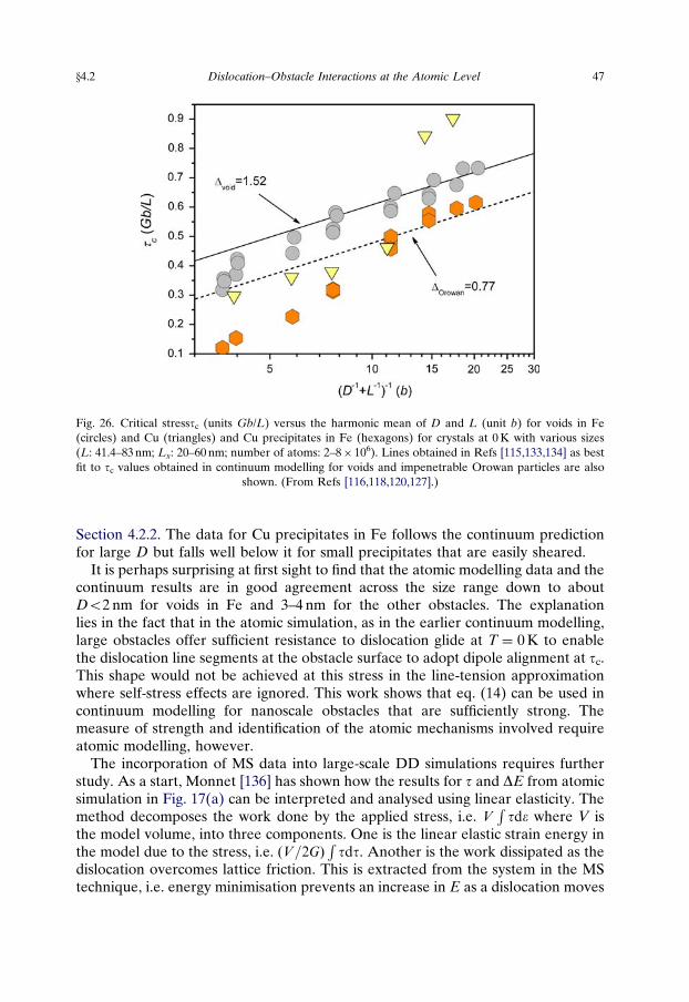
Section 4.2.2. The data for Cu precipitates in Fe follows the continuum predictionfor large D but falls well below it for small precipitates that are easily sheared.

It is perhaps surprising at first sight to find that the atomic modelling data and thecontinuum results are in good agreement across the size range down to aboutDo2 nm for voids in Fe and 3–4 nm for the other obstacles. The explanationlies in the fact that in the atomic simulation, as in the earlier continuum modelling,large obstacles offer sufficient resistance to dislocation glide at T ¼ 0 K to enablethe dislocation line segments at the obstacle surface to adopt dipole alignment at tc.This shape would not be achieved at this stress in the line-tension approximationwhere self-stress effects are ignored. This work shows that eq. (14) can be used incontinuum modelling for nanoscale obstacles that are sufficiently strong. Themeasure of strength and identification of the atomic mechanisms involved requireatomic modelling, however.

The incorporation of MS data into large-scale DD simulations requires furtherstudy. As a start, Monnet [136] has shown how the results for t and DE from atomicsimulation in Fig. 17(a) can be interpreted and analysed using linear elasticity. Themethod decomposes the work done by the applied stress, i.e. V

Rtd� where V is

the model volume, into three components. One is the linear elastic strain energy inthe model due to the stress, i.e. ðV=2GÞ

Rtdt. Another is the work dissipated as the

dislocation overcomes lattice friction. This is extracted from the system in the MStechnique, i.e. energy minimisation prevents an increase in E as a dislocation moves

Fig. 26. Critical stresstc (units Gb/L) versus the harmonic mean of D and L (unit b) for voids in Fe(circles) and Cu (triangles) and Cu precipitates in Fe (hexagons) for crystals at 0 K with various sizes(L: 41.4–83 nm; Lx: 20–60 nm; number of atoms: 2–8� 106). Lines obtained in Refs [115,133,134] as bestfit to tc values obtained in continuum modelling for voids and impenetrable Orowan particles are also

shown. (From Refs [116,118,120,127].)


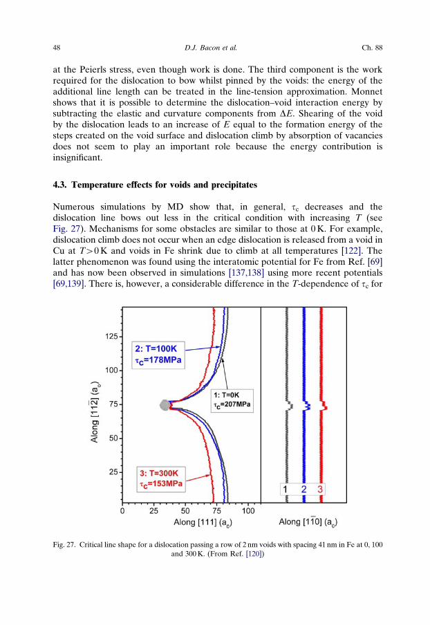
at the Peierls stress, even though work is done. The third component is the workrequired for the dislocation to bow whilst pinned by the voids: the energy of theadditional line length can be treated in the line-tension approximation. Monnetshows that it is possible to determine the dislocation–void interaction energy bysubtracting the elastic and curvature components from DE. Shearing of the voidby the dislocation leads to an increase of E equal to the formation energy of thesteps created on the void surface and dislocation climb by absorption of vacanciesdoes not seem to play an important role because the energy contribution isinsignificant.

4.3. Temperature effects for voids and precipitates

Numerous simulations by MD show that, in general, tc decreases and thedislocation line bows out less in the critical condition with increasing T (seeFig. 27). Mechanisms for some obstacles are similar to those at 0 K. For example,dislocation climb does not occur when an edge dislocation is released from a void inCu at TW0 K and voids in Fe shrink due to climb at all temperatures [122]. Thelatter phenomenon was found using the interatomic potential for Fe from Ref. [69]and has now been observed in simulations [137,138] using more recent potentials[69,139]. There is, however, a considerable difference in the T-dependence of tc for

Fig. 27. Critical line shape for a dislocation passing a row of 2 nm voids with spacing 41 nm in Fe at 0, 100and 300 K. (From Ref. [120])


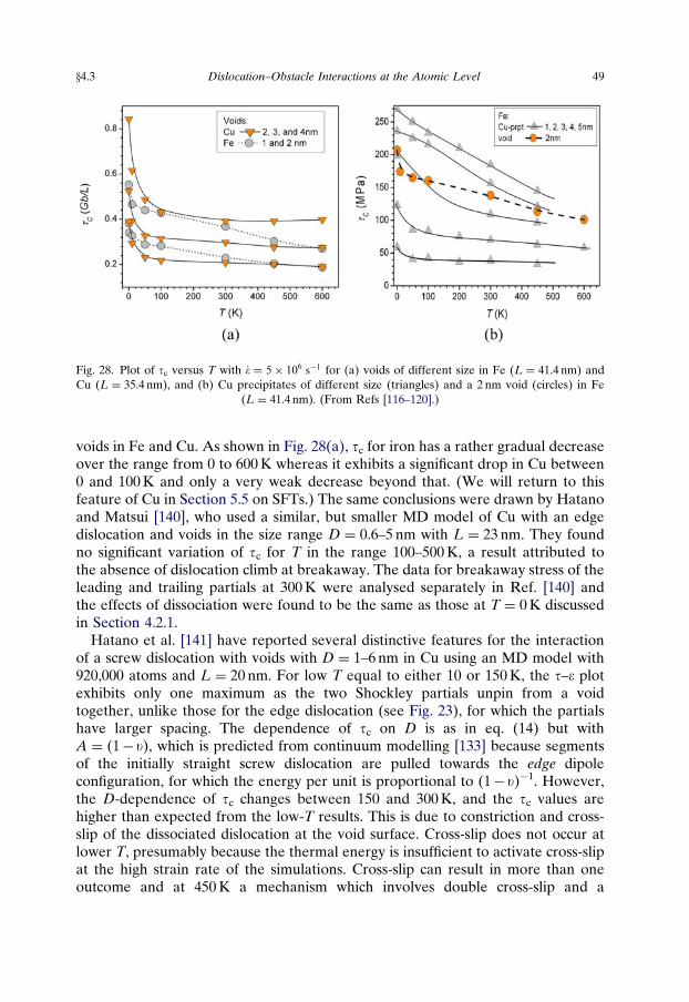
voids in Fe and Cu. As shown in Fig. 28(a), tc for iron has a rather gradual decreaseover the range from 0 to 600 K whereas it exhibits a significant drop in Cu between0 and 100 K and only a very weak decrease beyond that. (We will return to thisfeature of Cu in Section 5.5 on SFTs.) The same conclusions were drawn by Hatanoand Matsui [140], who used a similar, but smaller MD model of Cu with an edgedislocation and voids in the size range D ¼ 0.6–5 nm with L ¼ 23 nm. They foundno significant variation of tc for T in the range 100–500 K, a result attributed tothe absence of dislocation climb at breakaway. The data for breakaway stress of theleading and trailing partials at 300 K were analysed separately in Ref. [140] andthe effects of dissociation were found to be the same as those at T ¼ 0 K discussedin Section 4.2.1.

Hatano et al. [141] have reported several distinctive features for the interactionof a screw dislocation with voids with D ¼ 1–6 nm in Cu using an MD model with920,000 atoms and L ¼ 20 nm. For low T equal to either 10 or 150 K, the t–e plotexhibits only one maximum as the two Shockley partials unpin from a voidtogether, unlike those for the edge dislocation (see Fig. 23), for which the partialshave larger spacing. The dependence of tc on D is as in eq. (14) but withA ¼ (1� u), which is predicted from continuum modelling [133] because segmentsof the initially straight screw dislocation are pulled towards the edge dipoleconfiguration, for which the energy per unit is proportional to (1� u)�1. However,the D-dependence of tc changes between 150 and 300 K, and the tc values arehigher than expected from the low-T results. This is due to constriction and cross-slip of the dissociated dislocation at the void surface. Cross-slip does not occur atlower T, presumably because the thermal energy is insufficient to activate cross-slipat the high strain rate of the simulations. Cross-slip can result in more than oneoutcome and at 450 K a mechanism which involves double cross-slip and a

Fig. 28. Plot of tc versus T with _� ¼ 5� 106 s�1 for (a) voids of different size in Fe (L ¼ 41.4 nm) andCu (L ¼ 35.4 nm), and (b) Cu precipitates of different size (triangles) and a 2 nm void (circles) in Fe

(L ¼ 41.4 nm). (From Refs [116–120].)


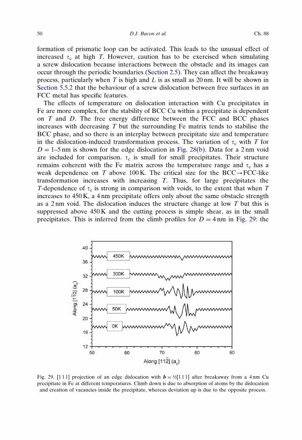
formation of prismatic loop can be activated. This leads to the unusual effect ofincreased tc at high T. However, caution has to be exercised when simulatinga screw dislocation because interactions between the obstacle and its images canoccur through the periodic boundaries (Section 2.5). They can affect the breakawayprocess, particularly when T is high and L is as small as 20 nm. It will be shown inSection 5.5.2 that the behaviour of a screw dislocation between free surfaces in anFCC metal has specific features.

The effects of temperature on dislocation interaction with Cu precipitates inFe are more complex, for the stability of BCC Cu within a precipitate is dependenton T and D. The free energy difference between the FCC and BCC phasesincreases with decreasing T but the surrounding Fe matrix tends to stabilise theBCC phase, and so there is an interplay between precipitate size and temperaturein the dislocation-induced transformation process. The variation of tc with T forD ¼ 1–5 nm is shown for the edge dislocation in Fig. 28(b). Data for a 2 nm voidare included for comparison. tc is small for small precipitates. Their structureremains coherent with the Fe matrix across the temperature range and tc has aweak dependence on T above 100 K. The critical size for the BCC-FCC-liketransformation increases with increasing T. Thus, for large precipitates theT-dependence of tc is strong in comparison with voids, to the extent that when Tincreases to 450 K, a 4 nm precipitate offers only about the same obstacle strengthas a 2 nm void. The dislocation induces the structure change at low T but this issuppressed above 450 K and the cutting process is simple shear, as in the smallprecipitates. This is inferred from the climb profiles for D ¼ 4 nm in Fig. 29: the

Fig. 29. [1 1 1] projection of an edge dislocation with b ¼ ½[1 1 1] after breakaway from a 4 nm Cuprecipitate in Fe at different temperatures. Climb down is due to absorption of atoms by the dislocationand creation of vacancies inside the precipitate, whereas deviation up is due to the opposite process.


phase transformation is accompanied by the creation of vacancies and extra atomsin the precipitate, resulting in dislocation climb seen for To450 K.

The size dependence of the Cu transformation mechanism has now beenconfirmed for screw dislocations by MD simulation of screw–precipitate interactionat 10 K under constant t [142]. It was observed that the phase transformationoccurred for DW1.8 nm and that when D exceeds 2.5 nm the dislocation bypassmechanism becomes Orowan looping due to the coherency loss of the precipitates.Values of tc were not obtained.

The simulations suggest that the yield stress of an under-aged or neutron-irradiated Fe–Cu alloy containing small, coherent precipitates should have a weakT-dependence, whereas the dependence should be stronger in an overaged orelectron-irradiated alloy where the population of coherent precipitates has largersize [127]. More direct experimental evidence in support of the simulation predic-tions has been obtained by Lozano-Perez et al. [143] by utilising the crystallographyof the BCC-9R martensitic transformation. Planes of atoms in twinned 9Rprecipitates exhibit characteristic ‘herring-bone’ fringe contrast when viewedalong a /1 1 1S direction of the Fe matrix in a high-resolution electron microscope(HREM). The angle, a, between fringes in neighbouring twin bands isapproximately 1291 immediately after the transformation, but relaxes duringannealing to 1211 to reduce the strain energy [123]. Samples of a Fe-1.3 wt%Cualloy were aged at 550 1C before cooling to room temperature, in order thatprecipitates larger than about 5 nm would transform to 9R whilst smallerprecipitates would retain the BCC structure. One set of samples was deformedby bending at room temperature and both sets were then annealed at 400 1C toallow transformed precipitates to relax. HREM foils were prepared at �60 1C sothat any remaining untransformed precipitates should transform to 9R. Angle awas then measured for precipitates in both sets of samples. The results are shownin Fig. 30, from which it is seen that precipitates in the undeformed alloy have arelaxation threshold of about 4–5 nm, while all the precipitates in the deformedsamples appear to be relaxed.

High-chromium (Cr) ferritic/martensitic steels offer another alloy system wherecoherent precipitates harden the material during ageing and/or irradiation. Cr-richau phase separates from the a phase and forms a fine dispersion of nanoscaleobstacles to dislocation motion, e.g. Refs [144–146]. Unlike Cu in Fe, Cr is stable inthe BCC structure, but it has a larger elastic modulus than Fe and au precipitates areexpected to repel dislocations, rather than attract them. Terentyev et al. [147] havesimulated the interaction of an edge dislocation with a row of spherical Crprecipitates in a matrix of either pure Fe or Fe–10at.% Cr, the latter being usedto compare the obstacle contributions of precipitates and a solid solution. The MSmethod (T ¼ 0 K) with the model in Ref. [42] described in Section 2.3 was usedwith the potential from Ref. [148]. The precipitate spacing was 14 nm for smallprecipitates (D ¼ 0.6 or 1.2 nm) and 28 nm for larger ones.

Examples of the critical line shape and corresponding stress–strain curvesobtained for several values of D are shown in Fig. 31. (The stress in the plot is theapplied stress minus 80 MPa, which is the Peierls stress at 0 K for the edge


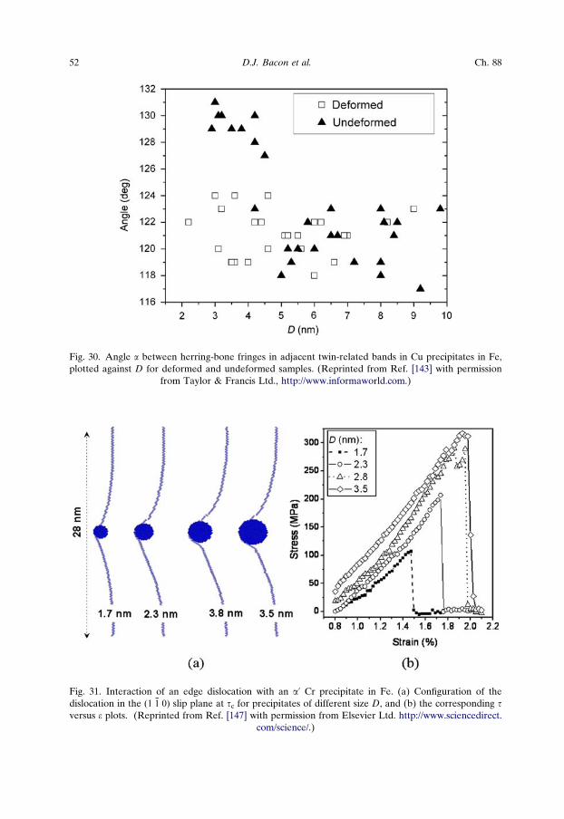
Fig. 30. Angle a between herring-bone fringes in adjacent twin-related bands in Cu precipitates in Fe,plotted against D for deformed and undeformed samples. (Reprinted from Ref. [143] with permission

from Taylor & Francis Ltd., http://www.informaworld.com.)

Fig. 31. Interaction of an edge dislocation with an au Cr precipitate in Fe. (a) Configuration of thedislocation in the ð1 �1 0Þ slip plane at tc for precipitates of different size D, and (b) the corresponding tversus e plots. (Reprinted from Ref. [147] with permission from Elsevier Ltd. http://www.sciencedirect.

com/science/.)


http://www.informaworld.com



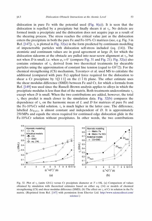
dislocation in pure Fe with the potential used (Fig. 8(a)). It is seen that thedislocation is repelled by a precipitate but finally shears it at tc. No defects areformed inside a precipitate and the dislocation does not acquire jogs as a result ofthe shearing process. The stress reaches the critical value just as the dislocationenters the precipitate in both the pure Fe and Fe-10% Cr matrices (see, e.g. Fig. 3 inRef. [147]). tc is plotted in Fig. 32(a) in the form predicted by continuum modellingof impenetrable particles with dislocation self-stress included (eq. (14)). Theatomistic and continuum values are in good agreement at large D, for which thedislocation sidearms at the obstacle are pulled into near-screw alignment at tc, butnot when D is small, i.e. when jcc01 (compare Fig. 31 and Fig. 21). Fig. 32(a) alsocontains estimates of tc derived from two theoretical treatments for shearableparticles using the approximation of constant line tension (equal to Gb2/2). For thechemical strengthening (CS) mechanism, Terentyev et al. used MS to calculate theadditional (compared with pure Fe) applied force required for the dislocation toshear a Cr precipitate by ½[1 1 1] on the ð1 �1 0Þ plane. The other estimate usesthe shear modulus difference (SMD) between Fe and Cr, for which a formula fromRef. [149] was used since the Russell–Brown analysis applies to alloys in which theprecipitate modulus is less than that of the matrix. Both treatments underestimate tc

except when D is small. When the two contributions are added, however, the totaltc they predict is much closer to the simulation data. Fig. 32(b) compares thedependence of tc on the harmonic mean of L and D for matrices of pure Fe andthe Fe-10%Cr solid solution. tc is much higher in the latter case. The difference,labelled DtFeCr, is almost constant and independent of D. It is approximately250 MPa and equals the stress required for continued edge dislocation glide in theFe-10%Cr solution without precipitates. In other words, the two contributions

Fig. 32. Plot of tc (units Gb/L) versus Cr precipitate diameter at T ¼ 0 K. (a) Comparison of valuesobtained by simulation with theoretical estimates based on either eq. (14) or models of chemicalstrengthening (CS) and shear modulus difference (SMD). (b) The effect on tc of Cr in solution in the Fematrix. (Reprinted from Ref. [147] with permission from Elsevier Ltd. http://www.sciencedirect.com/

science/.)




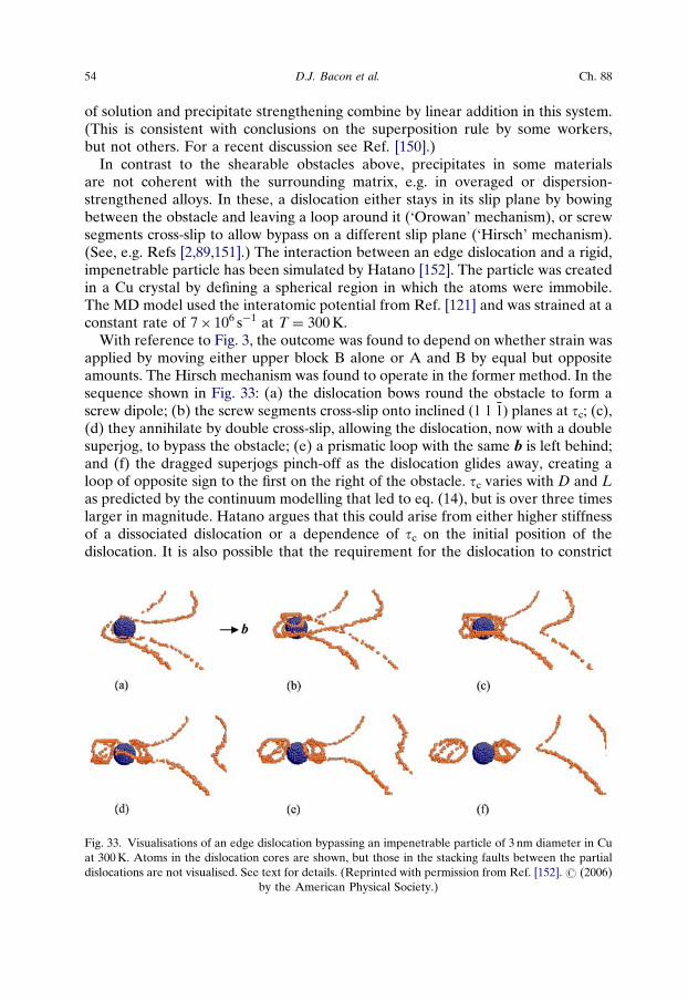
of solution and precipitate strengthening combine by linear addition in this system.(This is consistent with conclusions on the superposition rule by some workers,but not others. For a recent discussion see Ref. [150].)

In contrast to the shearable obstacles above, precipitates in some materialsare not coherent with the surrounding matrix, e.g. in overaged or dispersion-strengthened alloys. In these, a dislocation either stays in its slip plane by bowingbetween the obstacle and leaving a loop around it (‘Orowan’ mechanism), or screwsegments cross-slip to allow bypass on a different slip plane (‘Hirsch’ mechanism).(See, e.g. Refs [2,89,151].) The interaction between an edge dislocation and a rigid,impenetrable particle has been simulated by Hatano [152]. The particle was createdin a Cu crystal by defining a spherical region in which the atoms were immobile.The MD model used the interatomic potential from Ref. [121] and was strained at aconstant rate of 7� 106 s�1 at T ¼ 300 K.

With reference to Fig. 3, the outcome was found to depend on whether strain wasapplied by moving either upper block B alone or A and B by equal but oppositeamounts. The Hirsch mechanism was found to operate in the former method. In thesequence shown in Fig. 33: (a) the dislocation bows round the obstacle to form ascrew dipole; (b) the screw segments cross-slip onto inclined ð1 1 �1Þ planes at tc; (c),(d) they annihilate by double cross-slip, allowing the dislocation, now with a doublesuperjog, to bypass the obstacle; (e) a prismatic loop with the same b is left behind;and (f) the dragged superjogs pinch-off as the dislocation glides away, creating aloop of opposite sign to the first on the right of the obstacle. tc varies with D and Las predicted by the continuum modelling that led to eq. (14), but is over three timeslarger in magnitude. Hatano argues that this could arise from either higher stiffnessof a dissociated dislocation or a dependence of tc on the initial position of thedislocation. It is also possible that the requirement for the dislocation to constrict

Fig. 33. Visualisations of an edge dislocation bypassing an impenetrable particle of 3 nm diameter in Cuat 300 K. Atoms in the dislocation cores are shown, but those in the stacking faults between the partialdislocations are not visualised. See text for details. (Reprinted with permission from Ref. [152]. r (2006)

by the American Physical Society.)


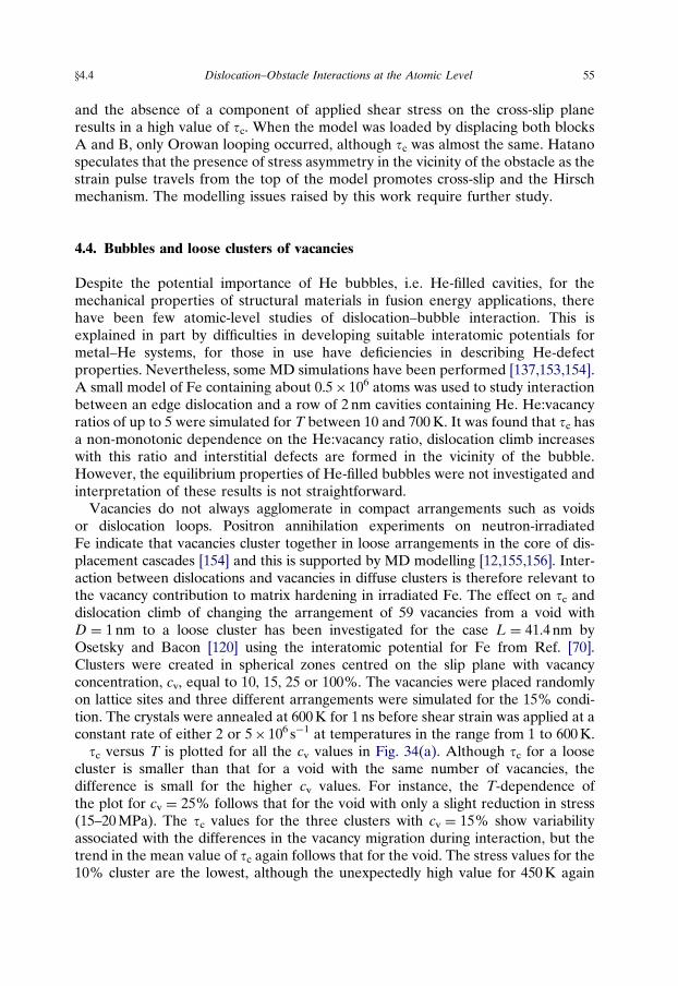
and the absence of a component of applied shear stress on the cross-slip planeresults in a high value of tc. When the model was loaded by displacing both blocksA and B, only Orowan looping occurred, although tc was almost the same. Hatanospeculates that the presence of stress asymmetry in the vicinity of the obstacle as thestrain pulse travels from the top of the model promotes cross-slip and the Hirschmechanism. The modelling issues raised by this work require further study.

4.4. Bubbles and loose clusters of vacancies

Despite the potential importance of He bubbles, i.e. He-filled cavities, for themechanical properties of structural materials in fusion energy applications, therehave been few atomic-level studies of dislocation–bubble interaction. This isexplained in part by difficulties in developing suitable interatomic potentials formetal–He systems, for those in use have deficiencies in describing He-defectproperties. Nevertheless, some MD simulations have been performed [137,153,154].A small model of Fe containing about 0.5� 106 atoms was used to study interactionbetween an edge dislocation and a row of 2 nm cavities containing He. He:vacancyratios of up to 5 were simulated for T between 10 and 700 K. It was found that tc hasa non-monotonic dependence on the He:vacancy ratio, dislocation climb increaseswith this ratio and interstitial defects are formed in the vicinity of the bubble.However, the equilibrium properties of He-filled bubbles were not investigated andinterpretation of these results is not straightforward.

Vacancies do not always agglomerate in compact arrangements such as voidsor dislocation loops. Positron annihilation experiments on neutron-irradiatedFe indicate that vacancies cluster together in loose arrangements in the core of dis-placement cascades [154] and this is supported by MD modelling [12,155,156]. Inter-action between dislocations and vacancies in diffuse clusters is therefore relevant tothe vacancy contribution to matrix hardening in irradiated Fe. The effect on tc anddislocation climb of changing the arrangement of 59 vacancies from a void withD ¼ 1 nm to a loose cluster has been investigated for the case L ¼ 41.4 nm byOsetsky and Bacon [120] using the interatomic potential for Fe from Ref. [70].Clusters were created in spherical zones centred on the slip plane with vacancyconcentration, cv, equal to 10, 15, 25 or 100%. The vacancies were placed randomlyon lattice sites and three different arrangements were simulated for the 15% condi-tion. The crystals were annealed at 600 K for 1 ns before shear strain was applied at aconstant rate of either 2 or 5� 106 s�1 at temperatures in the range from 1 to 600 K.

tc versus T is plotted for all the cv values in Fig. 34(a). Although tc for a loosecluster is smaller than that for a void with the same number of vacancies, thedifference is small for the higher cv values. For instance, the T-dependence ofthe plot for cv ¼ 25% follows that for the void with only a slight reduction in stress(15–20 MPa). The tc values for the three clusters with cv ¼ 15% show variabilityassociated with the differences in the vacancy migration during interaction, but thetrend in the mean value of tc again follows that for the void. The stress values for the10% cluster are the lowest, although the unexpectedly high value for 450 K again


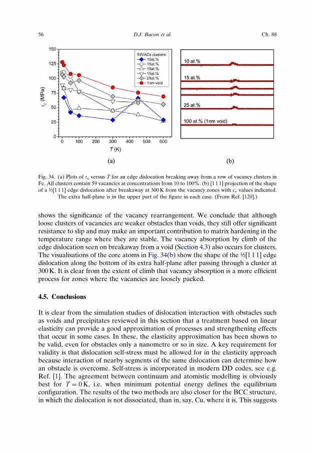
shows the significance of the vacancy rearrangement. We conclude that althoughloose clusters of vacancies are weaker obstacles than voids, they still offer significantresistance to slip and may make an important contribution to matrix hardening in thetemperature range where they are stable. The vacancy absorption by climb of theedge dislocation seen on breakaway from a void (Section 4.3) also occurs for clusters.The visualisations of the core atoms in Fig. 34(b) show the shape of the ½[1 1 1] edgedislocation along the bottom of its extra half-plane after passing through a cluster at300 K. It is clear from the extent of climb that vacancy absorption is a more efficientprocess for zones where the vacancies are loosely packed.

4.5. Conclusions

It is clear from the simulation studies of dislocation interaction with obstacles suchas voids and precipitates reviewed in this section that a treatment based on linearelasticity can provide a good approximation of processes and strengthening effectsthat occur in some cases. In these, the elasticity approximation has been shown tobe valid, even for obstacles only a nanometre or so in size. A key requirement forvalidity is that dislocation self-stress must be allowed for in the elasticity approachbecause interaction of nearby segments of the same dislocation can determine howan obstacle is overcome. Self-stress is incorporated in modern DD codes, see e.g.Ref. [1]. The agreement between continuum and atomistic modelling is obviouslybest for T ¼ 0 K, i.e. when minimum potential energy defines the equilibriumconfiguration. The results of the two methods are also closer for the BCC structure,in which the dislocation is not dissociated, than in, say, Cu, where it is. This suggests

Fig. 34. (a) Plots of tc versus T for an edge dislocation breaking away from a row of vacancy clusters inFe. All clusters contain 59 vacancies at concentrations from 10 to 100%. (b) [1 1 1] projection of the shapeof a ½[1 1 1] edge dislocation after breakaway at 300 K from the vacancy zones with cv values indicated.

The extra half-plane is in the upper part of the figure in each case. (From Ref. [120].)


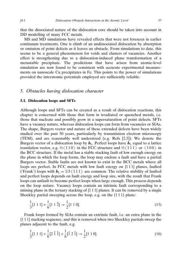
that the dissociated nature of the dislocation core should be taken into account inDD modelling of many FCC metals.

MS and MD simulations have revealed effects that were not foreseen in earliercontinuum treatments. One is climb of an undissociated dislocation by absorptionor emission of point defects as it leaves an obstacle. From simulations to date, thisseems to be a general phenomenon for voids and clusters of vacancies. Anothereffect is strengthening due to a dislocation-induced phase transformation of ametastable precipitate. The predictions that have arisen from atomic-levelsimulation are now found to be consistent with accurate experimental measure-ments on nanoscale Cu precipitates in Fe. This points to the power of simulationsprovided the interatomic potentials employed are sufficiently reliable.

5. Obstacles having dislocation character

5.1. Dislocation loops and SFTs

Although loops and SFTs can be created as a result of dislocation reactions, thischapter is concerned with those that form in irradiated or quenched metals, i.e.those that nucleate and possibly grow in a supersaturation of point defects. SFTshave a vacancy nature, whereas dislocation loops can form from vacancies or SIAs.The shape, Burgers vector and nature of these extended defects have been widelystudied over the past 50 years, particularly by transmission electron microscopy(TEM), and are reasonably well understood (e.g. Refs [2,3]). We denote theBurgers vector of a dislocation loop by bL. Perfect loops have bL equal to a latticetranslation vector, e.g. ½/1 1 0S in the FCC structure and ½/1 1 1S or /1 0 0S inthe BCC structure. If the metal has a stable stacking fault of low enough energy onthe plane in which the loop forms, the loop may enclose a fault and have a partialBurgers vector. Stable faults are not known to exist in the BCC metals where allloops are perfect. In FCC metals with low fault energy on {1 1 1} planes, faulted(‘Frank’) loops with bL ¼ 1/3/1 1 1S are common. The relative stability of faultedand perfect loops depends on fault energy and loop size, with the result that Frankloops can unfault to become perfect loops when large enough. This process dependson the loop nature. Vacancy loops contain an intrinsic fault corresponding to amissing plane in the ternary stacking of {1 1 1} planes. It can be removed by a singleShockley partial sweeping across the loop, e.g. on the (1 1 1) plane:

1

3½1 1 1� þ

1

6½1 1 �2� !

1

2½1 1 0�. (15)

Frank loops formed by SIAs contain an extrinsic fault, i.e. an extra plane in the{1 1 1} stacking sequence, and this is removed when two Shockley partials sweep theplanes adjacent to the fault, e.g.

1

3½1 1 1� þ

1

6½2 �1 �1� þ

1

6½�1 2 �1� !

1

2½1 1 0�. (16)


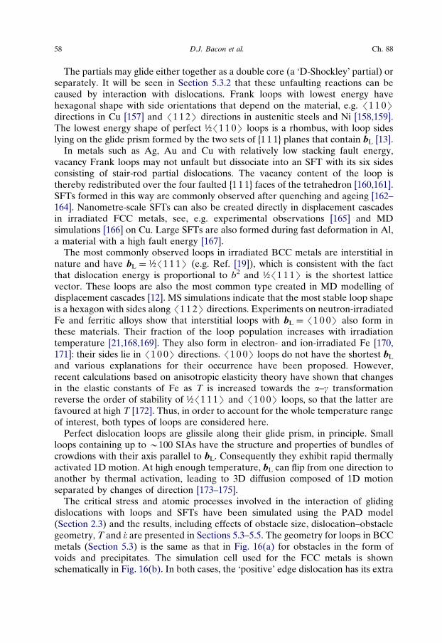
The partials may glide either together as a double core (a ‘D-Shockley’ partial) orseparately. It will be seen in Section 5.3.2 that these unfaulting reactions can becaused by interaction with dislocations. Frank loops with lowest energy havehexagonal shape with side orientations that depend on the material, e.g. /1 1 0Sdirections in Cu [157] and /1 1 2S directions in austenitic steels and Ni [158,159].The lowest energy shape of perfect ½/1 1 0S loops is a rhombus, with loop sideslying on the glide prism formed by the two sets of {1 1 1} planes that contain bL [13].

In metals such as Ag, Au and Cu with relatively low stacking fault energy,vacancy Frank loops may not unfault but dissociate into an SFT with its six sidesconsisting of stair-rod partial dislocations. The vacancy content of the loop isthereby redistributed over the four faulted {1 1 1} faces of the tetrahedron [160,161].SFTs formed in this way are commonly observed after quenching and ageing [162–164]. Nanometre-scale SFTs can also be created directly in displacement cascadesin irradiated FCC metals, see, e.g. experimental observations [165] and MDsimulations [166] on Cu. Large SFTs are also formed during fast deformation in Al,a material with a high fault energy [167].

The most commonly observed loops in irradiated BCC metals are interstitial innature and have bL ¼ ½/1 1 1S (e.g. Ref. [19]), which is consistent with the factthat dislocation energy is proportional to b2 and ½/1 1 1S is the shortest latticevector. These loops are also the most common type created in MD modelling ofdisplacement cascades [12]. MS simulations indicate that the most stable loop shapeis a hexagon with sides along /1 1 2S directions. Experiments on neutron-irradiatedFe and ferritic alloys show that interstitial loops with bL ¼ /1 0 0S also form inthese materials. Their fraction of the loop population increases with irradiationtemperature [21,168,169]. They also form in electron- and ion-irradiated Fe [170,171]: their sides lie in /1 0 0S directions. /1 0 0S loops do not have the shortest bL

and various explanations for their occurrence have been proposed. However,recent calculations based on anisotropic elasticity theory have shown that changesin the elastic constants of Fe as T is increased towards the a–g transformationreverse the order of stability of ½/1 1 1S and /1 0 0S loops, so that the latter arefavoured at high T [172]. Thus, in order to account for the whole temperature rangeof interest, both types of loops are considered here.

Perfect dislocation loops are glissile along their glide prism, in principle. Smallloops containing up to B100 SIAs have the structure and properties of bundles ofcrowdions with their axis parallel to bL. Consequently they exhibit rapid thermallyactivated 1D motion. At high enough temperature, bL can flip from one direction toanother by thermal activation, leading to 3D diffusion composed of 1D motionseparated by changes of direction [173–175].

The critical stress and atomic processes involved in the interaction of glidingdislocations with loops and SFTs have been simulated using the PAD model(Section 2.3) and the results, including effects of obstacle size, dislocation–obstaclegeometry, T and _� are presented in Sections 5.3–5.5. The geometry for loops in BCCmetals (Section 5.3) is the same as that in Fig. 16(a) for obstacles in the form ofvoids and precipitates. The simulation cell used for the FCC metals is shownschematically in Fig. 16(b). In both cases, the ‘positive’ edge dislocation has its extra


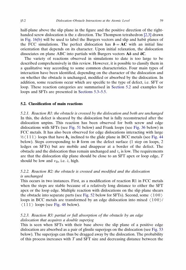
half-plane above the slip plane in the figure and the positive direction of the right-handed screw dislocation is the x direction. The Thompson tetrahedron [2,3] drawnin Fig. 16(b) will be used to label the Burgers vectors and slip and habit planes ofthe FCC simulations. The perfect dislocation has b ¼ AC with an initial lineorientation that depends on its character. Upon initial relaxation, the dislocationdissociates on plane ABC into partials with Burgers vectors Ad and dC.

The variety of reactions observed in simulations to date is too large to bedescribed comprehensively in this review. However, it is possible to classify them ina qualitative way according to some common characteristics. Four main types ofinteraction have been identified, depending on the character of the dislocation andon whether the obstacle is unchanged, modified or absorbed by the dislocation. Inaddition, some reactions occur which are specific to the type of defect, i.e. SFT orloop. These reaction categories are summarised in Section 5.2 and examples forloops and SFTs are presented in Sections 5.3–5.5.

5.2. Classification of main reactions

5.2.1. Reaction R1: the obstacle is crossed by the dislocation and both are unchangedIn this, the defect is sheared by the dislocation but is fully reconstructed after thedislocation unpins. This reaction has been observed for both screw and edgedislocations with SFTs (see Fig. 51 below) and Frank loops (see Fig. 36 below) inFCC metals. It has also been observed for edge dislocations interacting with large½/1 1 1S loops that have bL inclined to the glide plane in BCC metals (see Fig. 44below). Steps corresponding to b form on the defect surface (1 step on loops, 2ledges on SFTs) but are mobile and disappear at a border of the defect. Theobstacle and the dislocation thus remain unchanged and tc is low. The requirementsare that the dislocation slip plane should be close to an SFT apex or loop edge, Tshould be low and vD, i.e. _�, high.

5.2.2. Reaction R2: the obstacle is crossed and modified and the dislocationis unchangedThis occurs in two instances. First, as a modification of reaction R1 in FCC metalswhen the steps are stable because of a relatively long distance to either the SFTapex or the loop edge. Multiple reaction with dislocations on the slip plane shearsthe obstacle into separate parts (see Fig. 52 below for SFTs). Second, some /1 0 0Sloops in BCC metals are transformed by an edge dislocation into mixed /1 0 0S//1 1 1S loops (see Fig. 48 below).

5.2.3. Reaction R3: partial or full absorption of the obstacle by an edgedislocation that acquires a double superjogThis is seen when SFTs with their base above the slip plane of a positive edgedislocation are absorbed as a pair of glissile superjogs on the dislocation (see Fig. 53below). The superjogs can thus be dragged away by the dislocation. The probabilityof this process increases with T and SFT size and decreasing distance between the


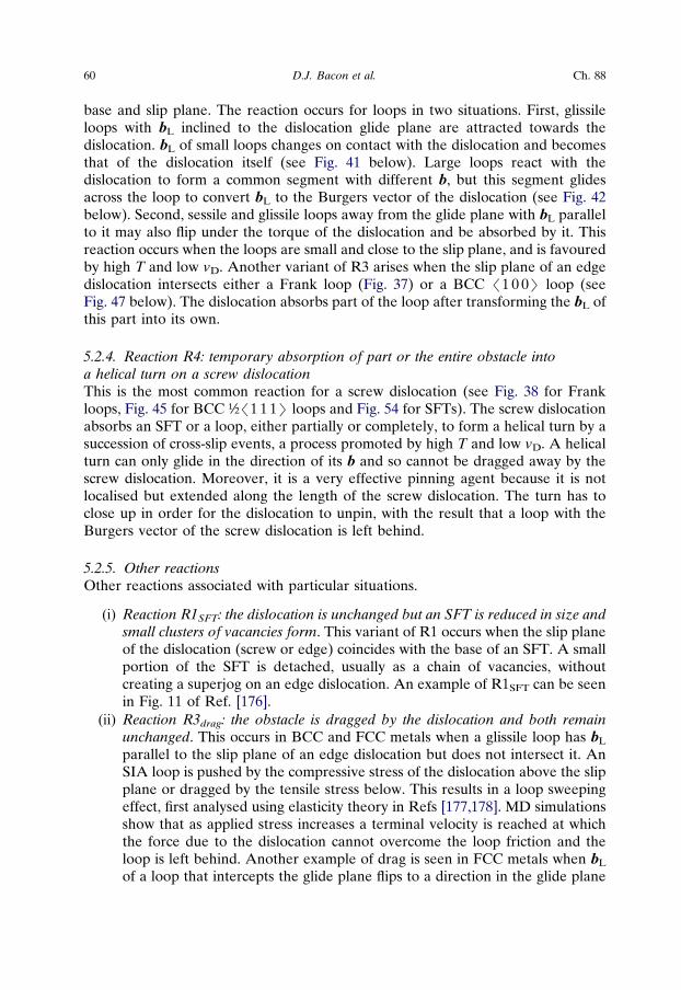
base and slip plane. The reaction occurs for loops in two situations. First, glissileloops with bL inclined to the dislocation glide plane are attracted towards thedislocation. bL of small loops changes on contact with the dislocation and becomesthat of the dislocation itself (see Fig. 41 below). Large loops react with thedislocation to form a common segment with different b, but this segment glidesacross the loop to convert bL to the Burgers vector of the dislocation (see Fig. 42below). Second, sessile and glissile loops away from the glide plane with bL parallelto it may also flip under the torque of the dislocation and be absorbed by it. Thisreaction occurs when the loops are small and close to the slip plane, and is favouredby high T and low vD. Another variant of R3 arises when the slip plane of an edgedislocation intersects either a Frank loop (Fig. 37) or a BCC /1 0 0S loop (seeFig. 47 below). The dislocation absorbs part of the loop after transforming the bL ofthis part into its own.

5.2.4. Reaction R4: temporary absorption of part or the entire obstacle intoa helical turn on a screw dislocationThis is the most common reaction for a screw dislocation (see Fig. 38 for Frankloops, Fig. 45 for BCC ½/1 1 1S loops and Fig. 54 for SFTs). The screw dislocationabsorbs an SFT or a loop, either partially or completely, to form a helical turn by asuccession of cross-slip events, a process promoted by high T and low vD. A helicalturn can only glide in the direction of its b and so cannot be dragged away by thescrew dislocation. Moreover, it is a very effective pinning agent because it is notlocalised but extended along the length of the screw dislocation. The turn has toclose up in order for the dislocation to unpin, with the result that a loop with theBurgers vector of the screw dislocation is left behind.

5.2.5. Other reactionsOther reactions associated with particular situations.

(i) Reaction R1SFT: the dislocation is unchanged but an SFT is reduced in size andsmall clusters of vacancies form. This variant of R1 occurs when the slip planeof the dislocation (screw or edge) coincides with the base of an SFT. A smallportion of the SFT is detached, usually as a chain of vacancies, withoutcreating a superjog on an edge dislocation. An example of R1SFT can be seenin Fig. 11 of Ref. [176].

(ii) Reaction R3drag: the obstacle is dragged by the dislocation and both remainunchanged. This occurs in BCC and FCC metals when a glissile loop has bL

parallel to the slip plane of an edge dislocation but does not intersect it. AnSIA loop is pushed by the compressive stress of the dislocation above the slipplane or dragged by the tensile stress below. This results in a loop sweepingeffect, first analysed using elasticity theory in Refs [177,178]. MD simulationsshow that as applied stress increases a terminal velocity is reached at whichthe force due to the dislocation cannot overcome the loop friction and theloop is left behind. Another example of drag is seen in FCC metals when bL

of a loop that intercepts the glide plane flips to a direction in the glide plane


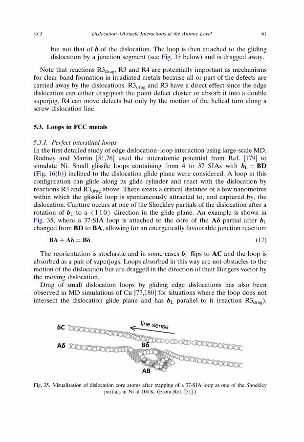
but not that of b of the dislocation. The loop is then attached to the glidingdislocation by a junction segment (see Fig. 35 below) and is dragged away.

Note that reactions R3drag, R3 and R4 are potentially important as mechanismsfor clear band formation in irradiated metals because all or part of the defects arecarried away by the dislocations. R3drag and R3 have a direct effect since the edgedislocation can either drag/push the point defect cluster or absorb it into a doublesuperjog. R4 can move defects but only by the motion of the helical turn along ascrew dislocation line.

5.3. Loops in FCC metals

5.3.1. Perfect interstitial loopsIn the first detailed study of edge dislocation–loop interaction using large-scale MD,Rodney and Martin [51,76] used the interatomic potential from Ref. [179] tosimulate Ni. Small glissile loops containing from 4 to 37 SIAs with bL ¼ BD(Fig. 16(b)) inclined to the dislocation glide plane were considered. A loop in thisconfiguration can glide along its glide cylinder and react with the dislocation byreactions R3 and R3drag above. There exists a critical distance of a few nanometreswithin which the glissile loop is spontaneously attracted to, and captured by, thedislocation. Capture occurs at one of the Shockley partials of the dislocation after arotation of bL to a /1 1 0S direction in the glide plane. An example is shown inFig. 35, where a 37-SIA loop is attached to the core of the Ad partial after bL

changed from BD to BA, allowing for an energetically favourable junction reaction:

BAþ Ad ¼ Bd. (17)

The reorientation is stochastic and in some cases bL flips to AC and the loop isabsorbed as a pair of superjogs. Loops absorbed in this way are not obstacles to themotion of the dislocation but are dragged in the direction of their Burgers vector bythe moving dislocation.

Drag of small dislocation loops by gliding edge dislocations has also beenobserved in MD simulations of Cu [77,180] for situations where the loop does notintersect the dislocation glide plane and has bL parallel to it (reaction R3drag).

Fig. 35. Visualisation of dislocation core atoms after trapping of a 37-SIA loop at one of the Shockleypartials in Ni at 100 K. (From Ref. [51].)


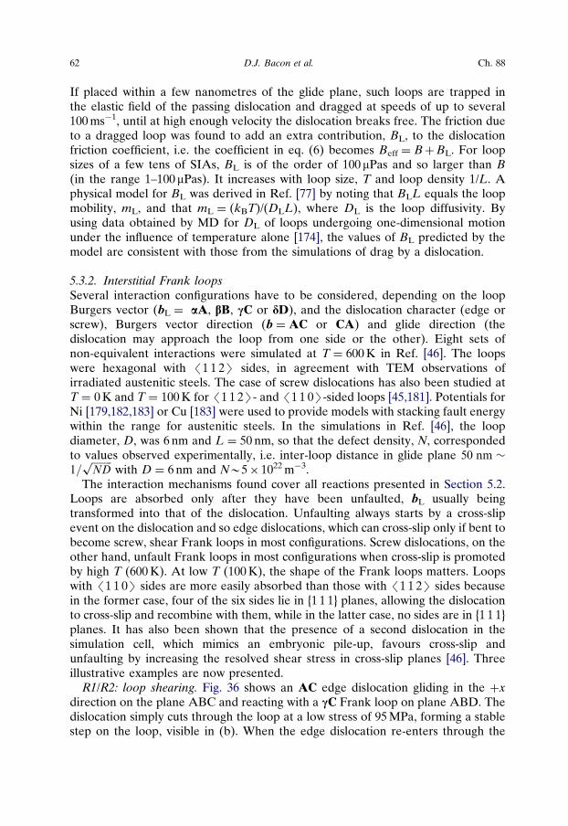
If placed within a few nanometres of the glide plane, such loops are trapped inthe elastic field of the passing dislocation and dragged at speeds of up to several100 ms�1, until at high enough velocity the dislocation breaks free. The friction dueto a dragged loop was found to add an extra contribution, BL, to the dislocationfriction coefficient, i.e. the coefficient in eq. (6) becomes Beff ¼ BþBL. For loopsizes of a few tens of SIAs, BL is of the order of 100 mPas and so larger than B(in the range 1–100 mPas). It increases with loop size, T and loop density 1/L. Aphysical model for BL was derived in Ref. [77] by noting that BLL equals the loopmobility, mL, and that mL ¼ (kBT)/(DLL), where DL is the loop diffusivity. Byusing data obtained by MD for DL of loops undergoing one-dimensional motionunder the influence of temperature alone [174], the values of BL predicted by themodel are consistent with those from the simulations of drag by a dislocation.

5.3.2. Interstitial Frank loopsSeveral interaction configurations have to be considered, depending on the loopBurgers vector (bL ¼ aA, bB, cC or dD), and the dislocation character (edge orscrew), Burgers vector direction (b ¼ AC or CA) and glide direction (thedislocation may approach the loop from one side or the other). Eight sets ofnon-equivalent interactions were simulated at T ¼ 600 K in Ref. [46]. The loopswere hexagonal with /1 1 2S sides, in agreement with TEM observations ofirradiated austenitic steels. The case of screw dislocations has also been studied atT ¼ 0 K and T ¼ 100 K for /1 1 2S- and /1 1 0S-sided loops [45,181]. Potentials forNi [179,182,183] or Cu [183] were used to provide models with stacking fault energywithin the range for austenitic steels. In the simulations in Ref. [46], the loopdiameter, D, was 6 nm and L ¼ 50 nm, so that the defect density, N, correspondedto values observed experimentally, i.e. inter-loop distance in glide plane 50 nm �1=

ffiffiffiffiffiffiffiffiNDp

with D ¼ 6 nm and NB5� 1022 m�3.The interaction mechanisms found cover all reactions presented in Section 5.2.

Loops are absorbed only after they have been unfaulted, bL usually beingtransformed into that of the dislocation. Unfaulting always starts by a cross-slipevent on the dislocation and so edge dislocations, which can cross-slip only if bent tobecome screw, shear Frank loops in most configurations. Screw dislocations, on theother hand, unfault Frank loops in most configurations when cross-slip is promotedby high T (600 K). At low T (100 K), the shape of the Frank loops matters. Loopswith /1 1 0S sides are more easily absorbed than those with /1 1 2S sides becausein the former case, four of the six sides lie in {1 1 1} planes, allowing the dislocationto cross-slip and recombine with them, while in the latter case, no sides are in {1 1 1}planes. It has also been shown that the presence of a second dislocation in thesimulation cell, which mimics an embryonic pile-up, favours cross-slip andunfaulting by increasing the resolved shear stress in cross-slip planes [46]. Threeillustrative examples are now presented.

R1/R2: loop shearing. Fig. 36 shows an AC edge dislocation gliding in the þxdirection on the plane ABC and reacting with a cC Frank loop on plane ABD. Thedislocation simply cuts through the loop at a low stress of 95 MPa, forming a stablestep on the loop, visible in (b). When the edge dislocation re-enters through the


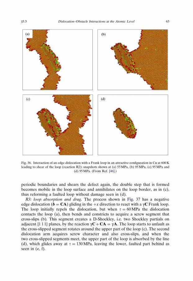
periodic boundaries and shears the defect again, the double step that is formedbecomes mobile in the loop surface and annihilates on the loop border, as in (c),thus reforming a faulted loop without damage seen in (d).

R3: loop absorption and drag. The process shown in Fig. 37 has a negativeedge dislocation (b ¼ CA) gliding in the þx direction to react with a cC Frank loop.The loop initially repels the dislocation, but when t ¼ 60 MPa the dislocationcontacts the loop (a), then bends and constricts to acquire a screw segment thatcross-slips (b). This segment creates a D-Shockley, i.e. two Shockley partials onadjacent {1 1 1} planes, by the reaction cCþCA ¼ cA. The loop starts to unfault asthe cross-slipped segment rotates around the upper part of the loop (c). The seconddislocation arm acquires screw character and also cross-slips, and when thetwo cross-slipped segments meet, the upper part of the loop is absorbed by the line(d), which glides away at t ¼ 130 MPa, leaving the lower, faulted part behind asseen in (e, f).

Fig. 36. Interaction of an edge dislocation with a Frank loop in an attractive configuration in Cu at 600 Kleading to shear of the loop (reaction R2): snapshots shown at (a) 55 MPa, (b) 95 MPa, (c) 95 MPa and

(d) 95 MPa. (From Ref. [46].)


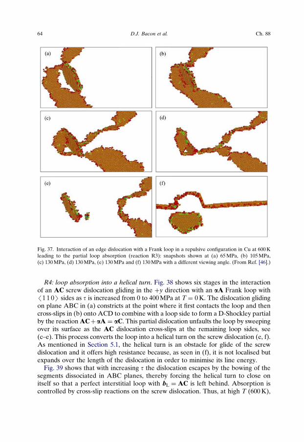
R4: loop absorption into a helical turn. Fig. 38 shows six stages in the interactionof an AC screw dislocation gliding in the þy direction with an aA Frank loop with/1 1 0S sides as t is increased from 0 to 400 MPa at T ¼ 0 K. The dislocation glidingon plane ABC in (a) constricts at the point where it first contacts the loop and thencross-slips in (b) onto ACD to combine with a loop side to form a D-Shockley partialby the reaction ACþ aA ¼ aC. This partial dislocation unfaults the loop by sweepingover its surface as the AC dislocation cross-slips at the remaining loop sides, see(c–e). This process converts the loop into a helical turn on the screw dislocation (e, f).As mentioned in Section 5.1, the helical turn is an obstacle for glide of the screwdislocation and it offers high resistance because, as seen in (f), it is not localised butexpands over the length of the dislocation in order to minimise its line energy.

Fig. 39 shows that with increasing t the dislocation escapes by the bowing of thesegments dissociated in ABC planes, thereby forcing the helical turn to close onitself so that a perfect interstitial loop with bL ¼ AC is left behind. Absorption iscontrolled by cross-slip reactions on the screw dislocation. Thus, at high T (600 K),

Fig. 37. Interaction of an edge dislocation with a Frank loop in a repulsive configuration in Cu at 600 Kleading to the partial loop absorption (reaction R3): snapshots shown at (a) 65 MPa, (b) 105 MPa,(c) 130 MPa, (d) 130 MPa, (e) 130 MPa and (f) 130 MPa with a different viewing angle. (From Ref. [46].)


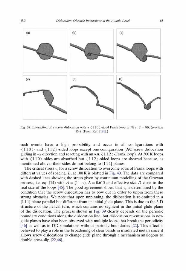
such events have a high probability and occur in all configurations with/1 1 0S- and /1 1 2S-sided loops except one configuration (AC screw dislocationgliding in –x direction and reacting with an aA /1 1 2S-Frank loop). At 300 K loopswith /1 1 0S sides are absorbed but /1 1 2S-sided loops are sheared because, asmentioned above, their sides do not belong to {1 1 1} planes.

The critical stress tc for a screw dislocation to overcome rows of Frank loops withdifferent values of spacing, L, at 100 K is plotted in Fig. 40. The data are comparedwith dashed lines showing the stress given by continuum modelling of the Orowanprocess, i.e. eq. (14) with A ¼ (1� n), D ¼ 0.615 and effective size D close to thereal size of the loops [45]. The good agreement shows that tc is determined by thecondition that the screw dislocation has to bow out in order to unpin from thesestrong obstacles. We note that upon unpinning, the dislocation is re-emitted in a{1 1 1} plane parallel but different from its initial glide plane. This is due to the 3-Dstructure of the helical turn, which contains no segment in the initial glide planeof the dislocation. The process shown in Fig. 39 clearly depends on the periodicboundary conditions along the dislocation line, but dislocation re-emissions in newglide planes have also been observed with multiple loops that break the periodicity[46] as well as in DD simulations without periodic boundaries [22]. This effect isbelieved to play a role in the broadening of clear bands in irradiated metals since itallows screw dislocations to change glide plane through a mechanism analogous todouble cross-slip [22,46].

Fig. 38. Interaction of a screw dislocation with a /1 1 0S-sided Frank loop in Ni at T ¼ 0 K (reactionR4). (From Ref. [181].)


5.4. Interstitial loops in BCC metals

5.4.1. ½/1 1 1S loopsDepending on the orientation of bL, two cases can be distinguished in theinteraction of a ½[1 1 1]ð1 �1 0Þ edge dislocation with ½/1 1 1S loops. First, two of thefour bL orientations, namely ½[1 1 1] and ½½1 1 �1�, are parallel to the dislocationglide plane and these loops can be dragged (reaction R3drag in Section 5.2). Thissituation was considered in Refs [180,184] for hexagonal loops containing either 37or 61 SIAs, with centres between 3 and 9 nm below the glide plane of the positiveedge dislocation. The process is as described in Section 5.3.1.

The second case concerns loops with bL ¼ ½½1 �1 1� and ½½�1 1 1� inclined to theglide plane. (They are equivalent for the ½[1 1 1]ð1 �1 0Þ dislocation.) Hexagonalloops with /1 1 2S sides and centres placed initially below the glide plane havebeen simulated for a variety of numbers of SIAs: 37 and 331 [184], 99 [185] and 169[186]. Sensitivity of results to the interatomic potential was examined by using thepotential of Ref. [69] in Ref. [184] and that of Ref. [70] in Ref. [186]. As mentionedin Section 5.1, ½/1 1 1S loops move easily by one-dimensional glide, and if withina few nanometres of a gliding edge dislocation, slip on their glide prism under

Fig. 39. Unpinning of a screw dislocation from a helical turn (reaction R4) at different times (in ps) in Niunder t ¼ 600 MPa at T ¼ 100 K: (a) 18, (b) 24, (c) 25.2 and (d) 27. (From Ref. [45].)


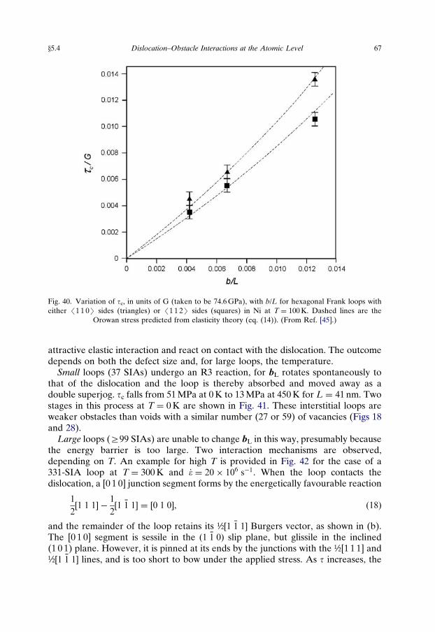
attractive elastic interaction and react on contact with the dislocation. The outcomedepends on both the defect size and, for large loops, the temperature.

Small loops (37 SIAs) undergo an R3 reaction, for bL rotates spontaneously tothat of the dislocation and the loop is thereby absorbed and moved away as adouble superjog. tc falls from 51 MPa at 0 K to 13 MPa at 450 K for L ¼ 41 nm. Twostages in this process at T ¼ 0 K are shown in Fig. 41. These interstitial loops areweaker obstacles than voids with a similar number (27 or 59) of vacancies (Figs 18and 28).

Large loops (Z99 SIAs) are unable to change bL in this way, presumably becausethe energy barrier is too large. Two interaction mechanisms are observed,depending on T. An example for high T is provided in Fig. 42 for the case of a331-SIA loop at T ¼ 300 K and _� ¼ 20� 106 s�1. When the loop contacts thedislocation, a [0 1 0] junction segment forms by the energetically favourable reaction

1

2½1 1 1� �

1

2½1 �1 1� ¼ ½0 1 0�, (18)

and the remainder of the loop retains its ½½1 �1 1� Burgers vector, as shown in (b).The [0 1 0] segment is sessile in the ð1 �1 0Þ slip plane, but glissile in the inclined(1 0 1) plane. However, it is pinned at its ends by the junctions with the ½[1 1 1] and½½1 �1 1� lines, and is too short to bow under the applied stress. As t increases, the

Fig. 40. Variation of tc, in units of G (taken to be 74.6 GPa), with b/L for hexagonal Frank loops witheither /1 1 0S sides (triangles) or /1 1 2S sides (squares) in Ni at T ¼ 100 K. Dashed lines are the

Orowan stress predicted from elasticity theory (eq. (14)). (From Ref. [45].)


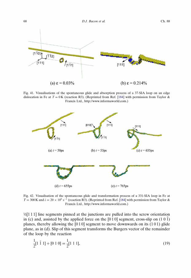
½[1 1 1] line segments pinned at the junctions are pulled into the screw orientationin (c) and, assisted by the applied force on the [0 1 0] segment, cross-slip on ð1 0 �1Þplanes, thereby allowing the [0 1 0] segment to move downwards on its (1 0 1) glideplane, as in (d). Slip of this segment transforms the Burgers vector of the remainderof the loop by the reaction

1

2½1 �1 1� þ ½0 1 0� ¼

1

2½1 1 1�, (19)

Fig. 41. Visualisations of the spontaneous glide and absorption process of a 37-SIA loop on an edgedislocation in Fe at T ¼ 0 K (reaction R3). (Reprinted from Ref. [184] with permission from Taylor &

Francis Ltd., http://www.informaworld.com.)

Fig. 42. Visualisation of the spontaneous glide and transformation process of a 331-SIA loop in Fe atT ¼ 300 K and _� ¼ 20� 106 s�1 (reaction R3). (Reprinted from Ref. [184] with permission from Taylor &

Francis Ltd., http://www.informaworld.com.)


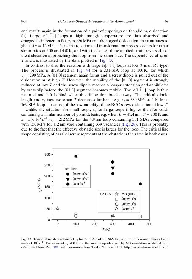
and results again in the formation of a pair of superjogs on the gliding dislocation(e). Large ½½1 �1 1� loops at high enough temperature are thus absorbed anddragged as in reaction R3. tc is 220 MPa and the jogged dislocation line continues toglide at t ¼ 12 MPa. The same reaction and transformation process occurs for otherstrain rates at 300 and 450 K, and with the sense of the applied strain reversed, i.e.the dislocation approaching the loop from the other side. The dependence of tc onT and _� is illustrated by the data plotted in Fig. 43.

In contrast to this, the reaction with large ½½1 �1 1� loops at low T is of R1 type.The process is illustrated in Fig. 44 for a 331-SIA loop at 100 K, for whichtc ¼ 290 MPa. A [0 1 0] segment again forms and a screw dipole is pulled out of thedislocation as at high T. However, the mobility of the [0 1 0] segment is stronglyreduced at low T and the screw dipole reaches a longer extension and annihilatesby cross-slip before the [0 1 0] segment becomes mobile. The ½½1 �1 1� loop is thusrestored and left behind when the dislocation breaks away. The critical dipolelength and tc increase when T decreases further – e.g. tc ¼ 530 MPa at 1 K for a169-SIA loop – because of the low mobility of the BCC screw dislocation at low T.

Unlike the situation for small loops, tc for large loops is higher than for voidscontaining a similar number of point defects, e.g. when L ¼ 41.4 nm, T ¼ 300 K and_� ¼ 5� 106 s�1, tc ¼ 212 MPa for the 4.9 nm loop containing 331 SIAs comparedwith 150 MPa for a 2 nm void containing 339 vacancies (Fig. 28). This is probablydue to the fact that the effective obstacle size is larger for the loop. The critical lineshape consisting of parallel screw segments at the obstacle is the same in both cases,

Fig. 43. Temperature dependence of tc for 37-SIA and 331-SIA loops in Fe for various values of _� inunits of 106 s�1. The value of tc at 0 K for the small loop obtained by MS simulation is also shown.(Reprinted from Ref. [184] with permission from Taylor & Francis Ltd., http://www.informaworld.com.)


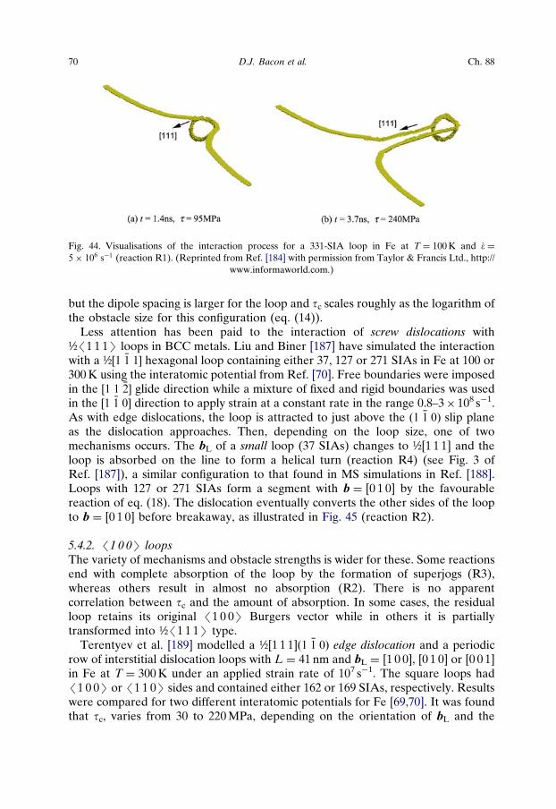
but the dipole spacing is larger for the loop and tc scales roughly as the logarithm ofthe obstacle size for this configuration (eq. (14)).

Less attention has been paid to the interaction of screw dislocations with½/1 1 1S loops in BCC metals. Liu and Biner [187] have simulated the interactionwith a ½½1 �1 1� hexagonal loop containing either 37, 127 or 271 SIAs in Fe at 100 or300 K using the interatomic potential from Ref. [70]. Free boundaries were imposedin the ½1 1 �2� glide direction while a mixture of fixed and rigid boundaries was usedin the ½1 �1 0� direction to apply strain at a constant rate in the range 0.8–3� 108 s�1.As with edge dislocations, the loop is attracted to just above the ð1 �1 0Þ slip planeas the dislocation approaches. Then, depending on the loop size, one of twomechanisms occurs. The bL of a small loop (37 SIAs) changes to ½[1 1 1] and theloop is absorbed on the line to form a helical turn (reaction R4) (see Fig. 3 ofRef. [187]), a similar configuration to that found in MS simulations in Ref. [188].Loops with 127 or 271 SIAs form a segment with b ¼ [0 1 0] by the favourablereaction of eq. (18). The dislocation eventually converts the other sides of the loopto b ¼ [0 1 0] before breakaway, as illustrated in Fig. 45 (reaction R2).

5.4.2. /1 0 0S loopsThe variety of mechanisms and obstacle strengths is wider for these. Some reactionsend with complete absorption of the loop by the formation of superjogs (R3),whereas others result in almost no absorption (R2). There is no apparentcorrelation between tc and the amount of absorption. In some cases, the residualloop retains its original /1 0 0S Burgers vector while in others it is partiallytransformed into ½/1 1 1S type.

Terentyev et al. [189] modelled a ½[1 1 1]ð1 �1 0Þ edge dislocation and a periodicrow of interstitial dislocation loops with L ¼ 41 nm and bL ¼ [1 0 0], [0 1 0] or [0 0 1]in Fe at T ¼ 300 K under an applied strain rate of 107 s�1. The square loops had/1 0 0S or /1 1 0S sides and contained either 162 or 169 SIAs, respectively. Resultswere compared for two different interatomic potentials for Fe [69,70]. It was foundthat tc, varies from 30 to 220 MPa, depending on the orientation of bL and the

Fig. 44. Visualisations of the interaction process for a 331-SIA loop in Fe at T ¼ 100 K and _� ¼5� 106 s�1 (reaction R1). (Reprinted from Ref. [184] with permission from Taylor & Francis Ltd., http://

www.informaworld.com.)


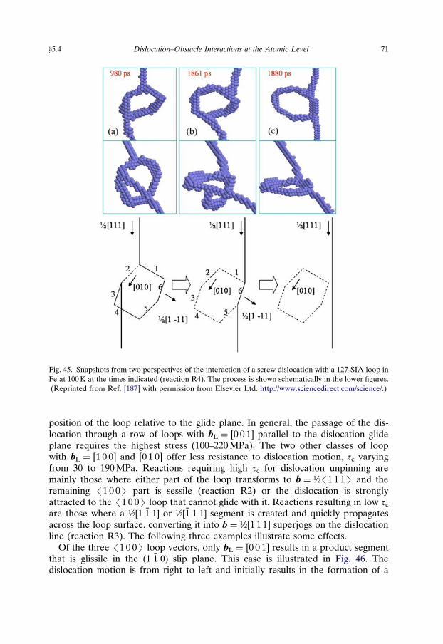
position of the loop relative to the glide plane. In general, the passage of the dis-location through a row of loops with bL ¼ [0 0 1] parallel to the dislocation glideplane requires the highest stress (100–220 MPa). The two other classes of loopwith bL ¼ [1 0 0] and [0 1 0] offer less resistance to dislocation motion, tc varyingfrom 30 to 190 MPa. Reactions requiring high tc for dislocation unpinning aremainly those where either part of the loop transforms to b ¼ ½/1 1 1S and theremaining /1 0 0S part is sessile (reaction R2) or the dislocation is stronglyattracted to the /1 0 0S loop that cannot glide with it. Reactions resulting in low tc

are those where a ½½1 �1 1� or ½½�1 1 1� segment is created and quickly propagatesacross the loop surface, converting it into b ¼ ½[1 1 1] superjogs on the dislocationline (reaction R3). The following three examples illustrate some effects.

Of the three /1 0 0S loop vectors, only bL ¼ [0 0 1] results in a product segmentthat is glissile in the ð1 �1 0Þ slip plane. This case is illustrated in Fig. 46. Thedislocation motion is from right to left and initially results in the formation of a

Fig. 45. Snapshots from two perspectives of the interaction of a screw dislocation with a 127-SIA loop inFe at 100 K at the times indicated (reaction R4). The process is shown schematically in the lower figures.(Reprinted from Ref. [187] with permission from Elsevier Ltd. http://www.sciencedirect.com/science/.)



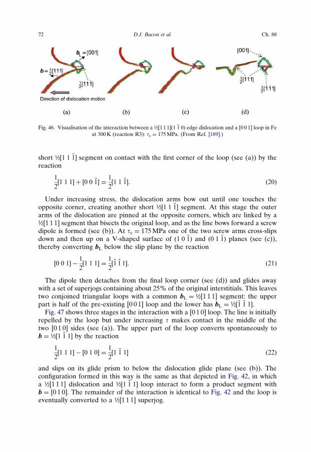
short ½½1 1 �1� segment on contact with the first corner of the loop (see (a)) by thereaction

1

2½1 1 1� þ ½0 0 �1� ¼

1

2½1 1 �1�. (20)

Under increasing stress, the dislocation arms bow out until one touches theopposite corner, creating another short ½½1 1 �1� segment. At this stage the outerarms of the dislocation are pinned at the opposite corners, which are linked by a½[1 1 1] segment that bisects the original loop, and as the line bows forward a screwdipole is formed (see (b)). At tc ¼ 175 MPa one of the two screw arms cross-slipsdown and then up on a V-shaped surface of ð1 0 �1Þ and ð0 1 �1Þ planes (see (c)),thereby converting bL below the slip plane by the reaction

½0 0 1� �1

2½1 1 1� ¼

1

2½�1 �1 1�. (21)

The dipole then detaches from the final loop corner (see (d)) and glides awaywith a set of superjogs containing about 25% of the original interstitials. This leavestwo conjoined triangular loops with a common bL ¼ ½[1 1 1] segment: the upperpart is half of the pre-existing [0 0 1] loop and the lower has bL ¼ ½½�1 �1 1�.

Fig. 47 shows three stages in the interaction with a [0 1 0] loop. The line is initiallyrepelled by the loop but under increasing t makes contact in the middle of thetwo [0 1 0] sides (see (a)). The upper part of the loop converts spontaneously tob ¼ ½½1 �1 1� by the reaction

1

2½1 1 1� � ½0 1 0� ¼

1

2½1 �1 1� (22)

and slips on its glide prism to below the dislocation glide plane (see (b)). Theconfiguration formed in this way is the same as that depicted in Fig. 42, in whicha ½[1 1 1] dislocation and ½½1 �1 1� loop interact to form a product segment withb ¼ [0 1 0]. The remainder of the interaction is identical to Fig. 42 and the loop iseventually converted to a ½[1 1 1] superjog.

Fig. 46. Visualisation of the interaction between a ½[1 1 1]ð1 �1 0Þ edge dislocation and a [0 0 1] loop in Feat 300 K (reaction R3): tc ¼ 175 MPa. (From Ref. [189].)


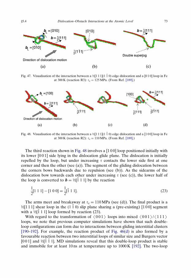
The third reaction shown in Fig. 48 involves a [1 0 0] loop positioned initially withits lower [0 0 1] side lying in the dislocation glide plane. The dislocation is initiallyrepelled by the loop, but under increasing t contacts the lower side first at onecorner and then the other (see (a)). The segment of the gliding dislocation betweenthe corners bows backwards due to repulsion (see (b)). As the sidearms of thedislocation bow towards each other under increasing t (see (c)), the lower half ofthe loop is converted to b ¼ ½½�1 1 1� by the reaction

1

2½1 1 1� � ½1 0 0� ¼

1

2½�1 1 1�. (23)

The arms meet and breakaway at tc ¼ 110 MPa (see (d)). The final product is a½[1 1 1] shear loop in the ð1 �1 0Þ slip plane sharing a (pre-existing) [1 0 0] segmentwith a ½½�1 1 1� loop formed by reaction (23).

With regard to the transformation of /0 0 1S loops into mixed /0 0 1S//1 1 1Sloops, we note that previous computer simulations have shown that such double-loop configurations can form due to interactions between gliding interstitial clusters[190–192]. For example, the reaction product of Fig. 46(d) is also formed by afavourable reaction between two interstitial loops of similar size and Burgers vector[0 0 1] and ½½�1 �1 1�. MD simulations reveal that this double-loop product is stableand immobile for at least 10 ns at temperature up to 1000 K [192]. The two-loop




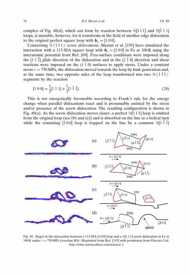
complex of Fig. 48(d), which can form by reaction between ½[1 1 1] and ½½�1 1 1�loops, is unstable, however, for it transforms in the field of another edge dislocationto the original perfect square loop with bL ¼ [1 0 0].

Concerning ½/1 1 1S screw dislocations, Marian et al. [193] have simulated theinteraction with a 113-SIA square loop with bL ¼ [1 0 0] in Fe at 100 K using theinteratomic potential from Ref. [69]. Free-surface conditions were imposed alongthe ½1 1 �2� glide direction of the dislocation and in the ½1 �1 0� direction and sheartractions were imposed on the ð1 �1 0Þ surfaces to apply stress. Under a constantstress t ¼ 750 MPa, the dislocation moved towards the loop by kink generation and,at the same time, two opposite sides of the loop transformed into two ½/1 1 1Ssegments by the reaction

½1 0 0� ¼1

2½1 1 1� þ

1

2½1 �1 �1�. (24)

This is not energetically favourable according to Frank’s rule for the energychange when parallel dislocations react and is presumably assisted by the stressand/or presence of the screw dislocation. The resulting configuration is shown inFig. 49(a). As the screw dislocation moves closer, a perfect ½[1 1 1] loop is emittedfrom the original loop (see (b) and (c)) and is absorbed on the line as a helical turnwhile the remaining [1 0 0] loop is trapped on the line by a common ½½1 �1 �1�

Fig. 49. Stages in the interaction between a 113-SIA [1 0 0] loop and a ½[1 1 1] screw dislocation in Fe at100 K under t ¼ 750 MPa (reaction R4). (Reprinted from Ref. [193] with permission from Elsevier Ltd.

http://www.sciencedirect.com/science/.)



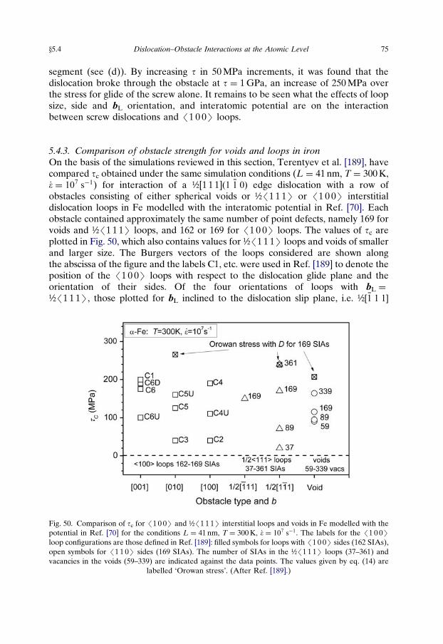
segment (see (d)). By increasing t in 50 MPa increments, it was found that thedislocation broke through the obstacle at t ¼ 1 GPa, an increase of 250 MPa overthe stress for glide of the screw alone. It remains to be seen what the effects of loopsize, side and bL orientation, and interatomic potential are on the interactionbetween screw dislocations and /1 0 0S loops.

5.4.3. Comparison of obstacle strength for voids and loops in ironOn the basis of the simulations reviewed in this section, Terentyev et al. [189], havecompared tc obtained under the same simulation conditions (L ¼ 41 nm, T ¼ 300 K,_� ¼ 107 s�1) for interaction of a ½[1 1 1]ð1 �1 0Þ edge dislocation with a row ofobstacles consisting of either spherical voids or ½/1 1 1S or /1 0 0S interstitialdislocation loops in Fe modelled with the interatomic potential in Ref. [70]. Eachobstacle contained approximately the same number of point defects, namely 169 forvoids and ½/1 1 1S loops, and 162 or 169 for /1 0 0S loops. The values of tc areplotted in Fig. 50, which also contains values for ½/1 1 1S loops and voids of smallerand larger size. The Burgers vectors of the loops considered are shown alongthe abscissa of the figure and the labels C1, etc. were used in Ref. [189] to denote theposition of the /1 0 0S loops with respect to the dislocation glide plane and theorientation of their sides. Of the four orientations of loops with bL ¼

½/1 1 1S, those plotted for bL inclined to the dislocation slip plane, i.e. ½½�1 1 1�

Fig. 50. Comparison of tc for /1 0 0S and ½/1 1 1S interstitial loops and voids in Fe modelled with thepotential in Ref. [70] for the conditions L ¼ 41 nm, T ¼ 300 K, _� ¼ 107 s�1. The labels for the /1 0 0Sloop configurations are those defined in Ref. [189]: filled symbols for loops with /1 0 0S sides (162 SIAs),open symbols for /1 1 0S sides (169 SIAs). The number of SIAs in the ½/1 1 1S loops (37–361) andvacancies in the voids (59–339) are indicated against the data points. The values given by eq. (14) are

labelled ‘Orowan stress’. (After Ref. [189].)


or ½½1 �1 1�, are relatively strong obstacles. The void of 169 vacancies is a weakerobstacle than either the ½/1 1 1S loops or some of the /1 0 0S loops containing thesame number of SIAs.

It should be borne in mind that loops and voids containing 169 point defects arenot fully representative of the size spectrum of point defect clusters in irradiatedmetals, and it is clear from the additional tc values for larger and smaller clustersplotted in Fig. 50 that the size-dependence of tc is different for loops and voids. Thedata for ½½1 �1 1� loops demonstrate a 10-fold increase in tc as the number ofinterstitials increases from 37 to 331. This is because smaller loops are readilyabsorbed as a pair of superjogs by spontaneous transformation of bL to ½[1 1 1].Larger loops react with the dislocation so that one side forms a common segmentwith b ¼ [0 1 0], which is sessile in the ð1 �1 0Þ plane and presents a strong obstacle.The obstacle strength of voids, in contrast, has a much weaker variation withnumber of vacancies because the mechanism of edge dislocation cutting andunpinning is not strongly dependent on diameter. As D increases, the dislocationbranches pinned at the void surface approach more closely to the screw orientation,and tc increases (see Section 4.2.1). As a result, voids are weaker obstacles thanmany loops when large, but stronger when small. Furthermore, the strength of voidshas weaker T-dependence than that of ½/1 1 1S loops [118,186]. All the tc dataobtained by MD simulation with T ¼ 300 K fall below the values predicted byeq. (14). The continuum approximation used for that equation mimics a crystal atT ¼ 0 K, i.e. no kinetic effects are considered. It was seen in Section 4.2.1 that tc

obtained by atomic-level simulation of void strengthening approaches the criticalvalue given by eq. (14) as T tends to 0 K if D is Z2 nm. Although the /1 0 0S loopsthat provide the strongest resistance, such as those labelled C1, C4, C6D and C6 inFig. 50, cause the dislocation sidearms to bow to the screw orientation as appliedstress increases, dislocation breakaway occurs before a stable screw dipole is drawnout. Thus, temperature (and possibly applied strain rate) affects the dislocationrelease mechanism and the measured obstacle strength falls below the theoreticallimit represented by eq. (14).

5.5. Stacking fault tetrahedra

5.5.1. Particular reactionsInteractions involving SFTs have been simulated extensively for both edge andscrew dislocations and a wide range of interactions was observed [49,118,176,194–199]. We present here examples of the main reaction types following the categoriesdescribed in Section 5.2. First, however, it is necessary to identify SFT-specificparameters that arise from the geometry of the interaction. The Thompsontetrahedron shown in Fig. 16(b) shows an SFT configuration. An SFT has twoorientations (Face and Edge) relative to the approaching dislocation and twoorientations of its apex (Up and Down) relative to the dislocation slip plane. Due tothe symmetry, all other arrangements, including the dislocation line sense, areequivalent to these. Therefore, the configuration shown in Fig. 16(b) can be


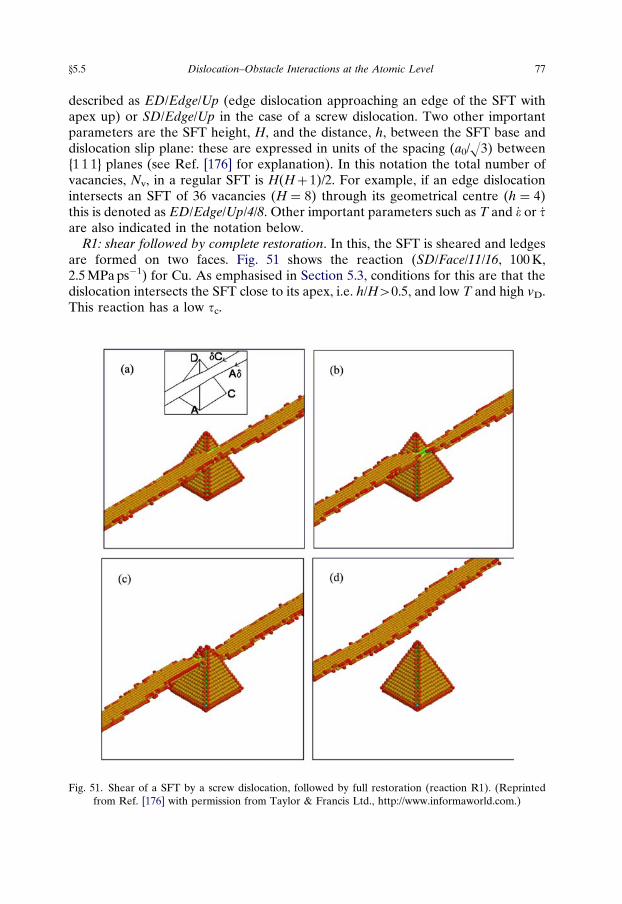
described as ED/Edge/Up (edge dislocation approaching an edge of the SFT withapex up) or SD/Edge/Up in the case of a screw dislocation. Two other importantparameters are the SFT height, H, and the distance, h, between the SFT base anddislocation slip plane: these are expressed in units of the spacing (a0/O3) between{1 1 1} planes (see Ref. [176] for explanation). In this notation the total number ofvacancies, Nv, in a regular SFT is H(Hþ 1)/2. For example, if an edge dislocationintersects an SFT of 36 vacancies (H ¼ 8) through its geometrical centre (h ¼ 4)this is denoted as ED/Edge/Up/4/8. Other important parameters such as T and _� or _tare also indicated in the notation below.

R1: shear followed by complete restoration. In this, the SFT is sheared and ledgesare formed on two faces. Fig. 51 shows the reaction (SD/Face/11/16, 100 K,2.5 MPa ps�1) for Cu. As emphasised in Section 5.3, conditions for this are that thedislocation intersects the SFT close to its apex, i.e. h/HW0.5, and low T and high vD.This reaction has a low tc.

Fig. 51. Shear of a SFT by a screw dislocation, followed by full restoration (reaction R1). (Reprintedfrom Ref. [176] with permission from Taylor & Francis Ltd., http://www.informaworld.com.)


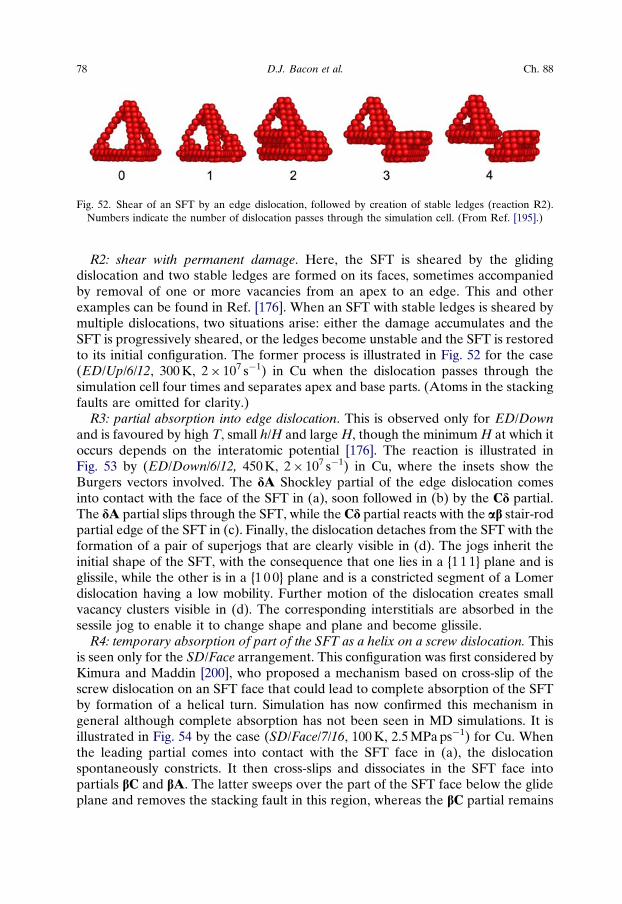
R2: shear with permanent damage. Here, the SFT is sheared by the glidingdislocation and two stable ledges are formed on its faces, sometimes accompaniedby removal of one or more vacancies from an apex to an edge. This and otherexamples can be found in Ref. [176]. When an SFT with stable ledges is sheared bymultiple dislocations, two situations arise: either the damage accumulates and theSFT is progressively sheared, or the ledges become unstable and the SFT is restoredto its initial configuration. The former process is illustrated in Fig. 52 for the case(ED/Up/6/12, 300 K, 2� 107 s�1) in Cu when the dislocation passes through thesimulation cell four times and separates apex and base parts. (Atoms in the stackingfaults are omitted for clarity.)

R3: partial absorption into edge dislocation. This is observed only for ED/Downand is favoured by high T, small h/H and large H, though the minimum H at which itoccurs depends on the interatomic potential [176]. The reaction is illustrated inFig. 53 by (ED/Down/6/12, 450 K, 2� 107 s�1) in Cu, where the insets show theBurgers vectors involved. The dA Shockley partial of the edge dislocation comesinto contact with the face of the SFT in (a), soon followed in (b) by the Cd partial.The dA partial slips through the SFT, while the Cd partial reacts with the ab stair-rodpartial edge of the SFT in (c). Finally, the dislocation detaches from the SFT with theformation of a pair of superjogs that are clearly visible in (d). The jogs inherit theinitial shape of the SFT, with the consequence that one lies in a {1 1 1} plane and isglissile, while the other is in a {1 0 0} plane and is a constricted segment of a Lomerdislocation having a low mobility. Further motion of the dislocation creates smallvacancy clusters visible in (d). The corresponding interstitials are absorbed in thesessile jog to enable it to change shape and plane and become glissile.

R4: temporary absorption of part of the SFT as a helix on a screw dislocation. Thisis seen only for the SD/Face arrangement. This configuration was first considered byKimura and Maddin [200], who proposed a mechanism based on cross-slip of thescrew dislocation on an SFT face that could lead to complete absorption of the SFTby formation of a helical turn. Simulation has now confirmed this mechanism ingeneral although complete absorption has not been seen in MD simulations. It isillustrated in Fig. 54 by the case (SD/Face/7/16, 100 K, 2.5 MPa ps�1) for Cu. Whenthe leading partial comes into contact with the SFT face in (a), the dislocationspontaneously constricts. It then cross-slips and dissociates in the SFT face intopartials bC and bA. The latter sweeps over the part of the SFT face below the glideplane and removes the stacking fault in this region, whereas the bC partial remains

Fig. 52. Shear of an SFT by an edge dislocation, followed by creation of stable ledges (reaction R2).Numbers indicate the number of dislocation passes through the simulation cell. (From Ref. [195].)


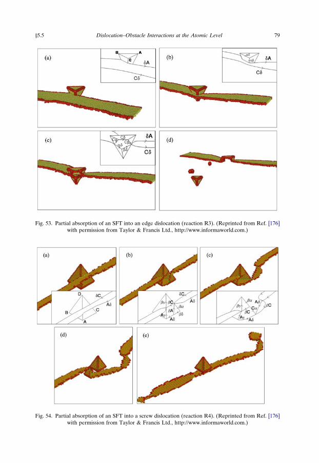
Fig. 53. Partial absorption of an SFT into an edge dislocation (reaction R3). (Reprinted from Ref. [176]with permission from Taylor & Francis Ltd., http://www.informaworld.com.)

Fig. 54. Partial absorption of an SFT into a screw dislocation (reaction R4). (Reprinted from Ref. [176]with permission from Taylor & Francis Ltd., http://www.informaworld.com.)


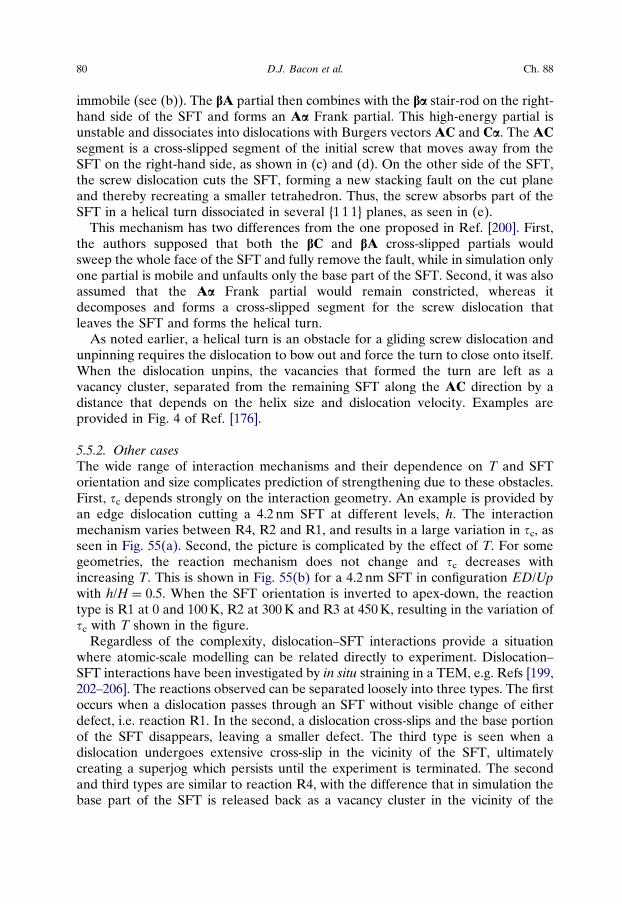
immobile (see (b)). The bA partial then combines with the ba stair-rod on the right-hand side of the SFT and forms an Aa Frank partial. This high-energy partial isunstable and dissociates into dislocations with Burgers vectors AC and Ca. The ACsegment is a cross-slipped segment of the initial screw that moves away from theSFT on the right-hand side, as shown in (c) and (d). On the other side of the SFT,the screw dislocation cuts the SFT, forming a new stacking fault on the cut planeand thereby recreating a smaller tetrahedron. Thus, the screw absorbs part of theSFT in a helical turn dissociated in several {1 1 1} planes, as seen in (e).

This mechanism has two differences from the one proposed in Ref. [200]. First,the authors supposed that both the bC and bA cross-slipped partials wouldsweep the whole face of the SFT and fully remove the fault, while in simulation onlyone partial is mobile and unfaults only the base part of the SFT. Second, it was alsoassumed that the Aa Frank partial would remain constricted, whereas itdecomposes and forms a cross-slipped segment for the screw dislocation thatleaves the SFT and forms the helical turn.

As noted earlier, a helical turn is an obstacle for a gliding screw dislocation andunpinning requires the dislocation to bow out and force the turn to close onto itself.When the dislocation unpins, the vacancies that formed the turn are left as avacancy cluster, separated from the remaining SFT along the AC direction by adistance that depends on the helix size and dislocation velocity. Examples areprovided in Fig. 4 of Ref. [176].

5.5.2. Other casesThe wide range of interaction mechanisms and their dependence on T and SFTorientation and size complicates prediction of strengthening due to these obstacles.First, tc depends strongly on the interaction geometry. An example is provided byan edge dislocation cutting a 4.2 nm SFT at different levels, h. The interactionmechanism varies between R4, R2 and R1, and results in a large variation in tc, asseen in Fig. 55(a). Second, the picture is complicated by the effect of T. For somegeometries, the reaction mechanism does not change and tc decreases withincreasing T. This is shown in Fig. 55(b) for a 4.2 nm SFT in configuration ED/Upwith h/H ¼ 0.5. When the SFT orientation is inverted to apex-down, the reactiontype is R1 at 0 and 100 K, R2 at 300 K and R3 at 450 K, resulting in the variation oftc with T shown in the figure.

Regardless of the complexity, dislocation–SFT interactions provide a situationwhere atomic-scale modelling can be related directly to experiment. Dislocation–SFT interactions have been investigated by in situ straining in a TEM, e.g. Refs [199,202–206]. The reactions observed can be separated loosely into three types. The firstoccurs when a dislocation passes through an SFT without visible change of eitherdefect, i.e. reaction R1. In the second, a dislocation cross-slips and the base portionof the SFT disappears, leaving a smaller defect. The third type is seen when adislocation undergoes extensive cross-slip in the vicinity of the SFT, ultimatelycreating a superjog which persists until the experiment is terminated. The secondand third types are similar to reaction R4, with the difference that in simulation thebase part of the SFT is released back as a vacancy cluster in the vicinity of the


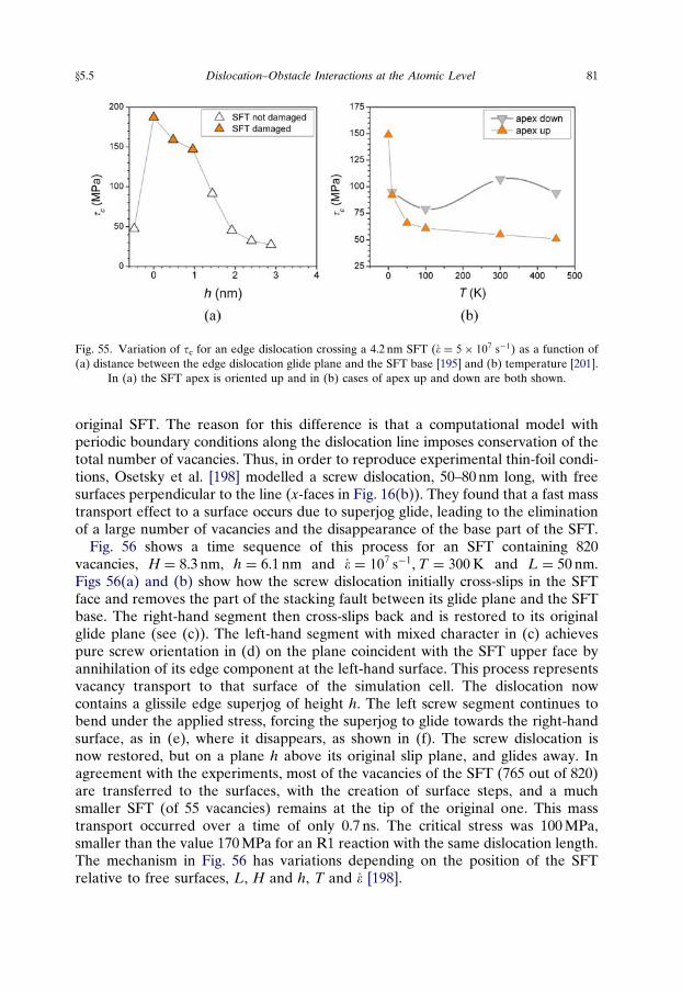
original SFT. The reason for this difference is that a computational model withperiodic boundary conditions along the dislocation line imposes conservation of thetotal number of vacancies. Thus, in order to reproduce experimental thin-foil condi-tions, Osetsky et al. [198] modelled a screw dislocation, 50–80 nm long, with freesurfaces perpendicular to the line (x-faces in Fig. 16(b)). They found that a fast masstransport effect to a surface occurs due to superjog glide, leading to the eliminationof a large number of vacancies and the disappearance of the base part of the SFT.

Fig. 56 shows a time sequence of this process for an SFT containing 820vacancies, H ¼ 8.3 nm, h ¼ 6.1 nm and _� ¼ 107 s�1;T ¼ 300K and L ¼ 50 nm.Figs 56(a) and (b) show how the screw dislocation initially cross-slips in the SFTface and removes the part of the stacking fault between its glide plane and the SFTbase. The right-hand segment then cross-slips back and is restored to its originalglide plane (see (c)). The left-hand segment with mixed character in (c) achievespure screw orientation in (d) on the plane coincident with the SFT upper face byannihilation of its edge component at the left-hand surface. This process representsvacancy transport to that surface of the simulation cell. The dislocation nowcontains a glissile edge superjog of height h. The left screw segment continues tobend under the applied stress, forcing the superjog to glide towards the right-handsurface, as in (e), where it disappears, as shown in (f). The screw dislocation isnow restored, but on a plane h above its original slip plane, and glides away. Inagreement with the experiments, most of the vacancies of the SFT (765 out of 820)are transferred to the surfaces, with the creation of surface steps, and a muchsmaller SFT (of 55 vacancies) remains at the tip of the original one. This masstransport occurred over a time of only 0.7 ns. The critical stress was 100 MPa,smaller than the value 170 MPa for an R1 reaction with the same dislocation length.The mechanism in Fig. 56 has variations depending on the position of the SFTrelative to free surfaces, L, H and h, T and _� [198].

Fig. 55. Variation of tc for an edge dislocation crossing a 4.2 nm SFT (_� ¼ 5� 107 s�1) as a function of(a) distance between the edge dislocation glide plane and the SFT base [195] and (b) temperature [201].

In (a) the SFT apex is oriented up and in (b) cases of apex up and down are both shown.


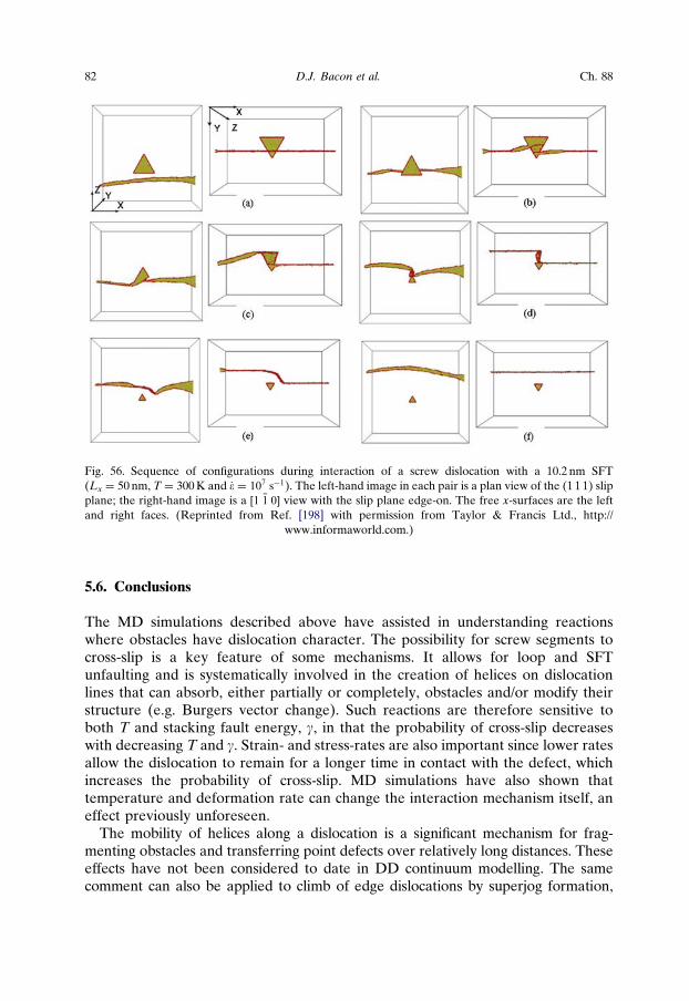
5.6. Conclusions

The MD simulations described above have assisted in understanding reactionswhere obstacles have dislocation character. The possibility for screw segments tocross-slip is a key feature of some mechanisms. It allows for loop and SFTunfaulting and is systematically involved in the creation of helices on dislocationlines that can absorb, either partially or completely, obstacles and/or modify theirstructure (e.g. Burgers vector change). Such reactions are therefore sensitive toboth T and stacking fault energy, g, in that the probability of cross-slip decreaseswith decreasing T and g. Strain- and stress-rates are also important since lower ratesallow the dislocation to remain for a longer time in contact with the defect, whichincreases the probability of cross-slip. MD simulations have also shown thattemperature and deformation rate can change the interaction mechanism itself, aneffect previously unforeseen.

The mobility of helices along a dislocation is a significant mechanism for frag-menting obstacles and transferring point defects over relatively long distances. Theseeffects have not been considered to date in DD continuum modelling. The samecomment can also be applied to climb of edge dislocations by superjog formation,

Fig. 56. Sequence of configurations during interaction of a screw dislocation with a 10.2 nm SFT(Lx ¼ 50 nm, T ¼ 300 K and _� ¼ 107 s�1). The left-hand image in each pair is a plan view of the (1 1 1) slipplane; the right-hand image is a ½1 �1 0� view with the slip plane edge-on. The free x-surfaces are the leftand right faces. (Reprinted from Ref. [198] with permission from Taylor & Francis Ltd., http://

www.informaworld.com.)


which has been shown here to be able to remove a significant fraction of dislocationobstacles. Climb is more effective for loops and SFTs than for voids and precipitates(Section 4), for which only a few defects are absorbed by a single dislocation.

The ability of atomic-scale simulation to reveal new mechanisms and provideinterpretation of experimental observations has been demonstrated in Section 5.5.2by the example of in situ TEM deformation. It is now clear that some reactionmechanisms that occur in thin films are specific to the conditions and cannot beapplied for bulk materials.

Finally, the dislocation obstacles considered here offer good examples whereatomic-scale modelling can interact productively with DD modelling by providingdetails of mechanisms and quantification of their parameters. The integration ofatomic and continuum treatments is a requirement for the development of a truemultiscale materials modelling approach to the effects of microstructure on mecha-nical properties. This has been done recently for Frank loops [22] but simula-tions involving all the details of the interaction mechanisms remain computationallyexpensive and more investigations are required on these issues.

6. Concluding remarks

Significant progress in applying atomic-scale simulation to problems of practicalimportance has been made over the past decade because of three factors. First, onthe hardware side the dramatic increase of computing power per unit of investmenthas allowed simulation of much larger models and also provided researchers withfacility to easily visualise the collective behaviour of hundreds or even thousandsof atoms. Second, computer codes have been improved by the development ofboundary conditions suitable for dislocations of different type and techniques forsimulating external loading, and this has led to more realistic modelling. Third,many new interatomic potentials have been produced with the use of ab initio data,and this development has increased confidence in the results of simulation.

As a result of these changes, MD and MS simulations can now be performed forobstacle microstructures with realistic length scale, defect size and dislocationdensity. We have shown that the parameters of current computer models are wellsuited to replication of microstructure created by radiation damage, which ischaracterised by a high density of nanometre-sized defects. Furthermore, atomic-scale simulations are now compatible with the scales of in situ deformation in aTEM, and so provide comparison between modelling and experiment, despite theshort timescale in the former and resolution limit in the latter.

The research reviewed here provides a broad view of individual dislocationinteraction with obstacles. Atomic-scale mechanisms such as absorption of defectsby edge dislocations that acquire superjogs, the formation of helical turns on screwdislocations with subsequent long-range mass transfer along dislocation lines, andcross-slip of screw dislocations (or screw parts on bowed edge dislocations) are keyfeatures of most interaction processes. The results obtained to date are sufficientlyextensive for us to have attempted a qualitative categorisation based on similarities


between the effects of different obstacles. These are most apparent for obstacleswith dislocation character, i.e. perfect dislocation loops in FCC and BCC metals,and faulted Frank loops and SFTs in FCC metals. (Although we have not discussedthem, effects such as loop absorption and transformation have also been found inthe few simulations that have been reported for the HCP structure [55,56].) Thesimilarities across crystal structures and defect types are consistent with changesobserved in all metals due to radiation damage, for phenomena such as hardening,embrittlement and clear band formation are common. It is particularly encouragingthat the well-established concepts of dislocation theory, based on linear elasticity,offer a valid interpretation of many of the effects observed for nanoscale obstacles,particularly with regard to the use of Frank’s rule for reaction between paralleldislocations and the influence of dislocation self-stress. This provides directvalidation of continuum DD simulations that use algorithms based on theseconcepts. The same conclusion has been made as a result of simulation of junctionformation between pairs of interacting dislocations [207–209].

There are still significant problems, however, that limit successful application ofatomic-scale techniques.

� Interatomic potentials. The realism of large-scale atomic simulations is dependenton the validity of interatomic potentials, which have to be short-ranged forcomputational efficiency and reproduce interactions between atoms in config-urations far from perfect. Validity remains limited for many metals. Potentials forrelatively simple metals are perhaps reliable, but those for transition metals,where electronic effects in bonding and magnetism are strong, are moreproblematic. Confidence in the simulated core structure of dislocations in someFCC metals is high, but the core of screw dislocations in BCC transition metals ishard to reproduce and the situation for HCP metals, in which the energy andstability of stacking faults on the basal and prism planes determines dislocationbehaviour, is no better. The development of potentials for alloys, where it isimportant to replicate local chemistry and thermodynamic properties, is also at anearly stage. Thus, it is wise to remember that most current potentials providemodels that have some of the properties of the real metals in question, such ascrystal structure, elastic constants, point defect energies, etc., but not all. Bycarrying out simulations with different potentials for the same metal, potential-specific peculiarities may be identified.� Timescale. This is possibly the most serious limitation of investigations based on

MD. Even with large supercomputers, the timescale accessible to MD simulationremains several orders of magnitude lower than that experienced in experiments,and this restricts the ability to study thermally activated processes. We havedemonstrated that MD simulations reproduce thermal effects, such as a decreaseof obstacle strength as T increases and an increase in the occurrence of cross-slipreactions when T increases and/or dislocation velocity decreases, i.e. when thestrain rate decreases. Nevertheless, thermally activated dislocation processes thatcan be observed in MD simulations have activation enthalpies smaller than 0.1 eVand most of the energy to overcome an obstacle is provided by the applied stress.


� Length scale. Despite clear successes in using atomic-scale models to studyinteractions between individual dislocations and small obstacles under a varietyof loading conditions, the creation of computational approaches capable ofpredicting mechanical behaviour due to microstructure changes resulting fromthermal or irradiation treatments is still a severe challenge. It demands not onlyatomic-level data based on longer times, but also knowledge of effects thatoperate over longer length scales. Examples include statistical effects of obstaclepopulations; cooperative dislocation effects such as pile-ups; mechanisms thataffect the operation and blocking of dislocation sources; the influence ofintergrain and interphase boundaries on dislocation motion; and the role of theseboundaries in acting as sources and sinks for dislocations and other defects.

We conclude that while application of massively parallelised, scalable models inthe near future may increase times and lengths, and reduce strain rates, by a feworders of magnitude, atomic-level simulation of millisecond and millimetre scaleswill not be achievable. Developments such as more efficient algorithms foraccelerated dynamics and saddle-point search methods to give access to thermallyactivated processes compatible with experiment will help, but not solve, theproblem. To exploit the power of atomic simulation, it will still be necessary to linkit to continuum-based DD modelling by using MD simulation to generate the localrules that describe dislocation–obstacle interaction. This provides the route to studythe effects mentioned in the previous paragraph. Although the variety ofmechanisms already revealed by MD is large, we have seen that it should bepossible to categorise them in such a way that they can be imported into DD codes.

Acknowledgements

Much of the work described in this chapter was carried out with support of grantsfrom a variety of sources, including grants GR/N23189/01, GR/R68870/01 and GR/S81162/01 from the UK Engineering and Physical Sciences Research Council; grantF160-CT-2003-508840 (‘PERFECT’) under programme EURATOM FP-6 of theEuropean Commission; and the Division of Materials Sciences and Engineering andthe Office of Fusion Energy Sciences, U.S. Department of Energy, under contractwith UT-Battelle, LLC. The authors thank Prof. Y. Brechet, and Drs. G. Martin,Y. Mastukawa, R.E. Stoller and S.J. Zinkle for many fruitful discussions ontheoretical modelling and experimental results, and Drs. T. Nogaret andD. Terentyev for their contributions to dislocation-loop simulations.

References

[1] V.V. Bulatov, W. Cai, Computer Simulations of Dislocations, Oxford University Press, Oxford,2006.

[2] D. Hull, D.J. Bacon, Introduction to Dislocations, Butterworth-Heinemann, Oxford, 2001.[3] J.P. Hirth, J. Lothe, Theory of Dislocations, Krieger Publishing Company, 1982.

Dislocation–Obstacle Interactions at the Atomic Level 85

[4] F.R.N. Nabarro, Theory of Crystal Dislocations, Oxford University Press, Oxford, 1967.[5] V. Vitek, V. Paidar, in: J.P. Hirth (Ed.), Dislocations in Solids, vol. 14, Elsevier, Amsterdam, 2008,

p. 439.[6] W. Cai, V.V. Bulatov, J. Chang, J. Li, S. Yip, in: F.R.N. Nabarro, J.P. Hirth (Eds.), Dislocations in

Solids, vol. 12, Elsevier, Amsterdam, 2004, p. 1.[7] H. Swygenhoven, P.M. Derlet, in: J.P. Hirth (Ed.), Dislocations in Solids, vol. 14, Elsevier,

Amsterdam, 2008, p. 1.[8] M. Finnis, Interatomic Forces in Condensed Matter, Oxford University Press, Oxford, 2003.[9] M.S. Daw, M.I. Baskes, Phys. Rev. B 29 (1984) 6443.

[10] M.P. Allen, D.J. Tildesley, Computer Simulation of Liquids, Oxford University Press, Oxford,1987.

[11] G.S. Was, Fundamentals of Radiation Materials Science, Springer, Berlin, 2007.[12] D.J. Bacon, Y.N. Osetsky, R. Stoller, R.E. Voskoboinikov, J. Nucl. Mater. 323 (2003) 152.[13] Y.N. Osetsky, D.J. Bacon, A. Serra, B.N. Singh, S.I. Golubov, J. Nucl. Mater. 276 (2000) 65.[14] Y.N. Osetsky, A. Serra, B.N. Singh, S.I. Golubov, Philos. Mag. A 80 (2000) 2131.[15] N. De Diego, Y.N. Osetsky, D.J. Bacon, J. Nucl. Mater. 374 (2008) 87.[16] J.V. Sharp, Philos. Mag. 16 (1967) 77.[17] F. Onimus, I. Monnet, J.L. Bechade, C. Prioul, P. Pilvin, J. Nucl. Mater. 328 (2004) 165.[18] M. Victoria, N. Baluc, C. Bailat, Y. Dai, M.I. Luppo, R. Schaublin, B.N. Singh, J. Nucl. Mater. 276

(2000) 114.[19] B.N. Singh, A. Horsewell, P. Toft, J. Nucl. Mater. 272 (1999) 97.[20] B.N. Singh, A. Horsewell, P. Toft, D.J. Edwards, J. Nucl. Mater. 224 (1995) 131.[21] S.J. Zinkle, B.N. Singh, J. Nucl. Mater. 351 (2006) 269.[22] T. Nogaret, D. Rodney, M. Fivel, C. Robertson, J. Nucl. Mater. 380 (2008) 22.[23] H.B. Huntington, J.E. Dickey, R. Thomson, Phys. Rev. 100 (1955) 1117.[24] R.M. Cotterill, M. Doyama, Phys. Rev. 145 (1966) 465.[25] R. Chang, L.J. Graham, Phys. Status Solidi 18 (1966) 99.[26] V. Vitek, R.C. Perrin, D.K. Bowen, Philos. Mag. 21 (1970) 1049.[27] J. Schiffgens, K.E. Garrison, J. Appl. Phys. 43 (1972) 3240.[28] R.C. Perrin, A. Englert, R. Bullough, in: P.C. Gehlen, J.R. Beeler, R.I. Jaffee (Eds.), Interatomic

Potentials and Simulation of Lattice Defects, Plenum Press, New York, 1972, p. 509.[29] V. Vitek, Cryst. Latt. Defects 5 (1974) 1.[30] M.S. Duesbery, V. Vitek, D.K. Bowen, Proc. R. Soc. Lond. A 332 (1973) 85.[31] S. Rao, C. Hernandez, J.P. Simmons, T.A. Parthasarathy, C. Woodward, Philos. Mag. A 77 (1998)

231.[32] V.B. Shenoy, R. Phillips, Philos. Mag. A 76 (1997) 367.[33] J.E. Sinclair, P.C. Gehlen, R.G. Hoagland, J.P. Hirth, J. Appl. Phys. 49 (1978) 3890.[34] R. Thomson, S.J. Zhou, A.E. Carlsson, V.K. Tewary, Phys. Rev. 46 (1992) 10613.[35] S.I. Golubov, X. Liu, H. Huang, C.H. Woo, Comput. Phys. Commun. 137 (2001) 312.[36] D.G. Pettifor, M. Aoki, Philos. Trans. R. Soc. Lond. A 334 (1991) 439.[37] J.A. Moriarty, V. Vitek, V.V. Bulatov, S. Yip, J. Comput. Aided Mater. Des. 9 (2002) 99.[38] C. Woodward, S.I. Rao, Phys. Rev. Lett. 88 (2002) 216402.[39] M.S. Daw, S.M. Foiles, M.I. Baskes, Mater. Sci. Rep. 9 (1993) 251.[40] R.C. Pond, J.P. Hirth, Solid State Phys. 47 (1994) 287.[41] A. Serra, D.J. Bacon, Y.N. Osetsky, Philos. Mag. Lett. 87 (2007) 451.[42] Y.N. Osetsky, D.J. Bacon, Modell. Simul. Mater. Sci. Eng. 11 (2003) 427.[43] C. Domain, G. Monnet, Phys. Rev. Lett. 95 (2005) 215506.[44] J. Chaussidon, M. Fivel, D. Rodney, Acta Mater. 54 (2006) 3407.[45] D. Rodney, Acta Mater. 52 (2004) 607.[46] T. Nogaret, C. Robertson, D. Rodney, Philos. Mag. 87 (2007) 945.[47] H.J. Lee, J.H. Shim, B.D. Wirth, J. Mater. Res. 22 (2007) 2758.[48] L. Saintoyant, H.J. Lee, B.D. Wirth, J. Nucl. Mater. 361 (2007) 206.[49] B.D. Wirth, V.V. Bulatov, T.D. De La Rubia, J. Eng. Mater. Technol. 124 (2002) 329.

86 D.J. Bacon et al.

[50] J. Marian, W. Cai, V.V. Bulatov, Nat. Mater. 3 (2004) 158.[51] D. Rodney, G. Martin, Phys. Rev. B 61 (2000) 8714.[52] E. Bitzek, P. Gumbsch, Mater. Sci. Eng. A 400–401 (2005) 40.[53] D. Rodney, Phys. Rev. B 76 (2007) 144108.[54] Y.N. Osetsky, S.I. Golubov (unpublished).[55] R.E. Voskoboinikov, Y.N. Osetsky, D.J. Bacon, Mater. Sci. Eng. A 400 (2005) 49.[56] R.E. Voskoboynikov, Y.N. Osetsky, D.J. Bacon, Mater. Sci. Eng. A 400 (2005) 54.[57] D. Terentyev, P. Grammatikopoulos, D.J. Bacon, Y.N. Osetsky, Acta Mater. 56 (2008) 5034.[58] J.D. Honeycutt, H.C. Andersen, J. Phys. Chem. 91 (1987) 4950.[59] J.C. Gil Montoro, J.L.F. Abascal, J. Phys. Chem. 97 (1993) 4211.[60] P. Guyot, J.E. Dorn, Can. J. Phys. 45 (1967) 983.[61] V. Vitek, Prog. Mater Sci. 36 (1992) 1.[62] C. Domain, J. Nucl. Mater. 351 (2006) 1.[63] S.L. Frederiksen, K.W. Jacobsen, Philos. Mag. 83 (2003) 365.[64] P.B. Hirsch, Proceedings of the 5th International Conference on Crystallography, Cambridge

University Press, Cambridge, 1960, p. 139.[65] L. Kubin, Rev. Deform. Behav. Mater. 244 (1977) 1.[66] H. Alexander, in: F.R.N. Nabarro (Ed.), Dislocations in Solids, vol. 7, Elsevier, Amsterdam, 1986,

p. 113.[67] D. Terentyev, D.J. Bacon, Y.N. Osetsky, J. Phys. Condens. Matter 20 (2008) 445007.[68] H. Khater, Ph.D. thesis, University of Liverpool, 2008.[69] G.J. Ackland, D.J. Bacon, A.F. Calder, T. Harry, Philos. Mag. A 75 (1997) 713.[70] G.J. Ackland, M.I. Mendelev, D.J. Srolovitz, S. Han, A.V. Barashev, J. Phys. Condens. Matter.

16 (2004) S2629.[71] G.J. Ackland, S.J. Wooding, D.J. Bacon, Philos. Mag. A 71 (1995) 553.[72] M.I. Mendelev, G.J. Ackland, Philos. Mag. Lett. 87 (2007) 349.[73] S. Takeuchi, Philos. Mag. A 39 (1979) 661.[74] J.L. Bassani, K. Ito, V. Vitek, Mater. Sci. Eng. A 319 (2001) 97.[75] V.I. Alshits, V.L. Indenbom, in: F.R.N. Nabarro, J.P. Hirth (Eds.), Dislocations in Solids, vol. 7,

Elsevier, Amsterdam, 1986, p. 43.[76] D. Rodney, G. Martin, Phys. Rev. Lett. 82 (1999) 3272.[77] Z. Rong, Y.N. Osetsky, D.J. Bacon, Philo. Mag. 85 (2005) 1473.[78] D.L. Olmsted, L.G. Hector, W.A. Curtin, R.J. Clifton, Modell. Simul. Mater. Sci. Eng. 13 (2005)

371.[79] A. Seeger, Philos. Mag. 1 (1956) 651.[80] J. Friedel, Dislocations, Pergamon Press, New York, 1964.[81] G. Henkelman, H. Jonsson, J. Chem. Phys. 111 (1999) 7010.[82] D. Brunner, J. Diehl, Phys. Status Solidi A 124 (1991) 455.[83] M. Tang, L.P. Kubin, G.R. Canova, Acta Mater. 46 (1998) 3221.[84] Y. Aono, K. Kitajima, E. Kuramoto, Scripta Metall. 15 (1981) 275.[85] Z.S. Basinski, M.S. Duesbery, G.S. Murty, Acta Metall. 29 (1981) 801.[86] M. Wen, A.H.W. Ngan, Acta Mater. 48 (2000) 4255.[87] R. Groger, V. Vitek, Philos. Mag. Lett. 87 (2007) 113.[88] A.S. Argon, Strengthening Mechanisms in Crystal Plasticity, Oxford University Press, Oxford,

2008.[89] J.W. Martin, Micromechanisms in Particle-Hardened Alloys, Cambridge University Press,

Cambridge, 1980.[90] A.J.E. Foreman, M.J. Makin, Philos. Mag. 14 (1966) 911.[91] U.F. Kocks, Can. J. Phys. 45 (1967) 737.[92] K. Hanson, J.W. Morris, J. Appl. Phys. 46 (1975) 983.[93] R. Labusch, J. Appl. Phys. 48 (1977) 4550.[94] M. Zaiser, Philos. Mag. A 82 (2002) 2869.[95] M. Hiratani, V.V. Bulatov, Philos. Mag. Lett. 84 (2004) 461.


[96] P. Haasen, in: F.R.N. Nabarro, J.P. Hirth (Eds.), Dislocations in Solids, vol. 4, Elsevier,Amsterdam, 1979, p. 155.

[97] D.R. Trinkle, C. Woodward, Science 310 (2005) 1665.[98] E. Rodary, D. Rodney, L. Proville, Y. Brechet, G. Martin, Phys. Rev. B 70 (2004) 054111.[99] K. Tapasa, D.J. Bacon, Y.N. Osetsky, Modell. Simul. Mater. Sci. Eng. 14 (2006) 1153.

[100] L. Proville, D. Rodney, Y. Brechet, G. Martin, Philos. Mag. 86 (2006) 3893.[101] S. Patinet, L. Proville, Phys. Rev. B 78 (2008) 104109.[102] R.W. Cahn, Nature 410 (2001) 643.[103] D.L. Olmsted, L.G. Hector, W.A. Curtin, J. Mech. Phys. Sol. 54 (2006) 1763.[104] T.H. Wille, W. Gieseke, C.H. Schwink, Acta Metall. 25 (1987) 2679.[105] A.H. Cottrell, B.A. Bilby, Phys. Soc. Lond. A 62 (1949) 49.[106] K. Tapasa, A.V. Barashev, D.J. Bacon, Y.N. Osetsky, Acta Mater. 55 (2007) 1.[107] R.A. Johnson, G.J. Dienes, A.C. Damask, Acta Metall. 12 (1964) 1215.[108] J.P. Hirth, M. Cohen, Scripta Metall. 3 (1969) 107.[109] J.P. Hirth, M. Cohen, Scripta Metall. 3 (1969) 311.[110] G. Schoeck, Scripta Metall. 3 (1969) 239.[111] D.J. Bacon, Scripta Metall. 3 (1969) 735.[112] C.S. Becquart, J.M. Raulot, G. Bencteux, C. Domain, M. Perez, S. Garruchet, H. Nguyen, Comput.

Mater. Sci. 40 (2007) 119.[113] R.E. Reed-Hill, R. Abbaschian, Physical Metallurgy Principles, PWS Publishing Company, Boston,

MA, 1991.[114] U.F. Kocks, A.S. Argon, M.F. Ashby, Thermodynamics and Kinetics of Slip, Prog. Mater. Sci. 19

(1975) (Pergamon, Oxford).[115] R.O. Scattergood, D.J. Bacon, Acta Metall. 30 (1982) 1665.[116] Y.N. Osetsky, D.J. Bacon, V. Mohles, Philos. Mag. 83 (2003) 3623.[117] Y.N. Osetsky, D.J. Bacon, J. Nucl. Mater. 323 (2003) 268.[118] D.J. Bacon, Y.N. Osetsky, JOM 59 (2007) 42.[119] D.J. Bacon, Y.N. Osetsky, J. Math. Mech. Sol. 14 (2009) 270.[120] Y.N. Osetsky, D.J. Bacon (unpublished).[121] G.J. Ackland, G.I. Tichy, V. Vitek, M.W. Finnis, Philos. Mag. A 56 (1987) 735.[122] D.J. Bacon, Y.N. Osetsky, Mater. Sci. Eng. A 400 (2005) 353.[123] R. Monzen, M.L. Jenkins, A.P. Sutton, Philos. Mag. A 80 (2000) 711.[124] J.T. Buswell, C.A. English, M.G. Hetherington, W.J. Phythian, G.D.W. Smith, G.M. Worral,

Effects of Radiation on Materials: 14th International Symposium ASTM STP 1046, vol. II, ASTM,Philadelphia, PA, 1990, p. 127.

[125] R.G. Carter, N. Soneda, K. Dohi, J.M. Hyde, C.A. English, W.L. Server, J. Nucl. Mater. 298 (2001)211.

[126] R. Chaouadi, R. Gerard, J. Nucl. Mater. 345 (2005) 65.[127] D.J. Bacon, Y.N. Osetsky, J. Nucl. Mater. 329–333 (2004) 1233.[128] Y.N. Osetsky, D.J. Bacon, in: H. Kitagawa, Y. Shibutani (Eds.), IUTAM Symposium on

Mesoscopic Dynamics of Fracture Process and Materials Strength, Kluwer Academic Publishers,Dordrecht, 2004, p. 193.

[129] Y.N. Osetsky, D.J. Bacon, Mater. Sci. Eng. A 400 (2005) 374.[130] T. Harry, D.J. Bacon, Acta Mater. 50 (2002) 195.[131] T. Harry, D.J. Bacon, Acta Mater. 50 (2002) 209.[132] K.C. Russell, L.M. Brown, Acta Metall. 20 (1972) 969.[133] D.J. Bacon, U.F. Kocks, R.O. Scattergood, Philos. Mag. 28 (1973) 1241.[134] R.O. Scattergood, D.J. Bacon, Philos. Mag. 31 (1975) 179.[135] D.J. Bacon, in: B.A. Bilby, K.J. Miller, J.R. Willis (Eds.), Fundamentals of Deformation and

Fracture, Cambridge University Press, Cambridge, 1985, p. 401.[136] G. Monnet, Acta Mater. 55 (2007) 5081.[137] R. Schaublin, N. Baluc, Nucl. Fusion 47 (2007) 1690.[138] S.M. Hafez Haghighat, R. Schaublin, J. Comput. Aided Mater. Des. 14 (2007) 191.


[139] S.L. Dudarev, P.M. Derlet, J. Phys. Condens. Matter 17 (2005) 7097.[140] T. Hatano, H. Matsui, Phys. Rev. 72 (2005) 094105.[141] T. Hatano, T. Kaneko, Y. Abe, H. Matsui, Phys. Rev. 77 (2008) 064108.[142] J.H. Shim, Y.W. Cho, S.C. Kwon, W.W. Kim, B.D. Wirth, Appl. Phys. Lett. 90 (2007) 021906.[143] S. Lozano-Perez, M.L. Jenkins, J.M. Titchmarsh, Philos. Mag. Lett. 86 (2006) 367.[144] K. Suganuma, H. Kayano, J. Nucl. Mater. 118 (1983) 234.[145] M.H. Mathon, Y. De Carlan, G. Geoffroy, X. Averty, A. Alamo, C.H. De Novion, J. Nucl. Mater.

312 (2003) 236.[146] A. Alamo, V. Lambard, X. Averty, M.H. Mathon, J. Nucl. Mater. 329–333 (2004) 333.[147] D.A. Terentyev, G. Bonny, L. Malerba, Acta Mater. 56 (2008) 3229.[148] P. Olsson, J. Wallenius, C. Domain, K. Nordlund, L. Malerba, Phys. Rev. B 72 (2005) 214119.[149] P.M. Kelly, Int. Metall. Rev. 18 (1973).[150] U. Lagerpusch, V. Mohles, E. Nembach, Mater. Sci. Eng. A 319–321 (2001) 176.[151] P.B. Hirsch, F.J. Humphreys, in: A.S. Argon (Ed.), Physics of Strength and Plasticity, MIT Press,

Boston, MA, 1969, p. 189.[152] T. Hatano, Phys. Rev. 74 (2006) 020102(R).[153] R. Schaublin, Y.L. Chiu, J. Nucl. Mater. 362 (2007) 152.[154] M. Eldrup, B.N. Singh, J. Nucl. Mater. 323 (2003) 346.[155] A.F. Calder, D.J. Bacon, J. Nucl. Mater. 207 (1993) 25.[156] A.F. Calder, D.J. Bacon, A.V. Barashev, Y.N. Osetsky, Philos. Mag. Lett. 88 (2008) 43.[157] M. Kiritani, H. Takata, J. Nucl. Mater. 69–70 (1978) 277.[158] M. Suzuki, A. Sato, T. Mori, J. Nagakawa, N. Yamamoto, H. Shiraishi, Philos. Mag. A 65 (1992)

1309.[159] L. Boulanger, F. Soisson, Y. Serruys, J. Nucl. Mater. 233–237 (1996) 1004.[160] Y.N. Osetsky, A. Serra, M. Victoria, S.I. Golubov, V. Priego, Philos. Mag. A 79 (1999) 2259.[161] Y.N. Osetsky, A. Serra, M. Victoria, S.I. Golubov, V. Priego, Philos. Mag. A 79 (1999) 2285.[162] J. Silcox, P.B. Hirsch, Philos. Mag. 4 (1959) 72.[163] M. Kiritani, J. Nucl. Mater. 216 (1994) 220.[164] S. Kojima, Y. Satoh, H. Taok, I. Ishida, T. Yoshiie, M. Kiritani, Philos. Mag. A 59 (1999) 519.[165] B.N. Singh, D.J. Edwards, P. Toft, J. Nucl. Mater. 299 (2001) 205.[166] R.E. Voskoboinikov, Y.N. Osetsky, D.J. Bacon, J. Nucl. Mater. 377 (2008) 385.[167] M. Kiritani, Y. Satoy, Y. Kizuka, K. Arakawa, Y. Ogasawara, S. Arai, Y. Shimomura, Philos. Mag.

Lett. 79 (1999) 797.[168] I.M. Robertson, M.L. Jenkins, C.A. English, J. Nucl. Mater. 108 (1982) 209.[169] L.L. Horton, J. Bentley, K. Farrell, J. Nucl. Mater. 108 (1982) 222.[170] B.C. Masters, Philos. Mag. 11 (1965) 881.[171] E.A. Little, B.L. Eyre, J. Micros. 97 (1973) 107.[172] S.L. Dudarev, R. Bullough, P.M. Derlet, Phys. Rev. Lett. 100 (2008) 135503.[173] N.V. Doan, D. Rodney, G. Martin, Diffusions in Materials: DIMAT 2000, Pts. 1 & 2, 194–199,

2001, p. 43.[174] Y.N. Osetsky, D.J. Bacon, A. Serra, B.N. Singh, S.I. Golubov, Philos. Mag. 83 (2003) 61.[175] K. Arakawa, K. Ono, M. Isshiki, K. Mimura, M. Uchikoshi, H. Mori, Science 318 (2007) 956.[176] Y.N. Osetsky, D. Rodney, D.J. Bacon, Philos. Mag. 86 (2006) 2295.[177] M.J. Makin, Philos. Mag. 10 (1964) 695.[178] L.P. Kubin, J. Kratochvil, Philos. Mag. A 80 (2000) 201.[179] J.E. Angelo, N.R. Moody, M.I. Baskes, Modell. Simul. Mater. Sci. Eng. 3 (1995) 289.[180] Y.N. Osetsky, D.J. Bacon, Z. Rong, B.N. Singh, Philos. Mag. Lett. 84 (2004) 745.[181] D. Rodney, Nucl. Instrum. Methods Phys. Res. Sect. B 228 (2005) 100.[182] Y. Mishin, D. Farkas, M.J. Mehl, D.A. Papaconstantopoulos, Phys. Rev. 59 (1999) 3393.[183] Y. Mishin, M.J. Mehl, D.A. Papaconstantopoulos, A.F. Voter, J.D. Kress, Phys. Rev. 63 (2001)

224106.[184] D.J. Bacon, Y.N. Osetsky, Z. Rong, Philos. Mag. 86 (2006) 3921.[185] A. Nomoto, N. Soneda, A. Takahashi, S. Ishino, Mater. Trans. JIM 46 (2005) 463.


[186] D. Terentyev, L. Malerba, D.J. Bacon, Y.N. Osetsky, J. Phys. Condens. Matter 19 (2007) 456211.[187] X.Y. Liu, S.B. Biner, Scripta Mater. 59 (2008) 51.[188] S. Jumel, J.C. Van Duysen, J. Ruste, C. Domain, J. Nucl. Mater. 346 (2005) 79.[189] D. Terentyev, D.J. Bacon, Y.N. Osetsky, Acta Mater. 56 (2008) 5034.[190] J. Marian, B.D. Wirth, J.M. Perlado, Phys. Rev. Lett. 88 (2002) 255507.[191] Y.N. Osetsky, A. Serra, V. Priego, J. Nucl. Mater. 276 (2000) 202.[192] D. Terentyev, L. Malerba, P. Klaver, P. Olsson, J. Nucl. Mater. 382 (2008) 126.[193] J. Marian, B.D. Wirth, R. Schaublin, G.R. Odette, J.M. Perlado, J. Nucl. Mater. 323 (2003) 181.[194] Y.N. Osetsky, D.J. Bacon, B.N. Singh, B. Wirth, J. Nucl. Mater. 307 (2002) 852.[195] Y.N. Osetsky, R.E. Stoller, Y. Matsukawa, J. Nucl. Mater. 329–333 (2004) 1228.[196] Y.N. Osetsky, R.E. Stoller, D. Rodney, D.J. Bacon, Mater. Sci. Eng. A 400 (2005) 370.[197] P. Szelestey, M. Patriarca, K. Kaski, Modell. Simul. Mater. Sci. Eng. 13 (2005) 541.[198] Y.N. Osetsky, Y. Matsukawa, R.E. Stoller, S.J. Zinkle, Philos. Mag. Lett. 86 (2006) 511.[199] J.S. Robach, I.M. Robertson, H.J. Lee, B.D. Wirth, Acta Mater. 54 (2006) 1679.[200] H. Kimura, R. Maddin, in: R.M.J. Cotterill, M. Dotama, J.J. Jackson, M. Meshii (Eds.), Lattice

Defects in Quenched Metals, Academic Press, New York, 1965, p. 319.[201] Y.N. Osetsky (unpublished).[202] J.S. Robach, I.M. Robertson, B.D. Wirth, A. Arsenlis, Philos. Mag. 83 (2003) 955.[203] Y. Matsukawa, S.J. Zinkle, J. Nucl. Mater. 329–333 (2004) 919.[204] Y. Matsukawa, Y.N. Osetsky, R.E. Stoller, S.J. Zinkle, Mater. Sci. Eng. A 400–401 (2005) 366.[205] Y. Matsukawa, Y.N. Osetsky, R.E. Stoller, S.J. Zinkle, J. Nucl. Mater. 351 (2006) 285.[206] Y. Matsukawa, Y.N. Osetsky, R.E. Stoller, S.J. Zinkle, Philos. Mag. 88 (2008) 581.[207] V. Bulatov, F.F. Abraham, L. Kubin, B. Devincre, S. Yip, Nature 391 (1998) 669.[208] R. Madec, B. Devincre, L. Kubin, T. Hoc, D. Rodney, Science 301 (2003) 1879.[209] V.V. Bulatov, L.L. Hsiung, M. Tang, A. Arsenlis, M.C. Bartelt, W. Cai, J.N. Florando, M. Hiratani,

M. Rhee, G. Hommes, T.G. Pierce, T.D. De La Rubia, Nature 440 (2006) 1174.


dislocation–obstacle interactions at the atomic level

Documents