Disorder-generated multifractalsand Random Matrices:

freezing phenomena and extremes 1

Yan V Fyodorov

School of Mathematical Sciences

Project supported by the EPSRC grant EP/J002763/1

1Based on: YVF, P Le Doussal and A Rosso J Stat Phys: 149 (2012), 898-920YVF, G Hiary, J Keating Phys. Rev. Lett. 108 , 170601 (2012) & arXiv:1211.6063YVF, B. A. Khoruzhenko and N. Simm in preparation

Disorder-generated multifractals:

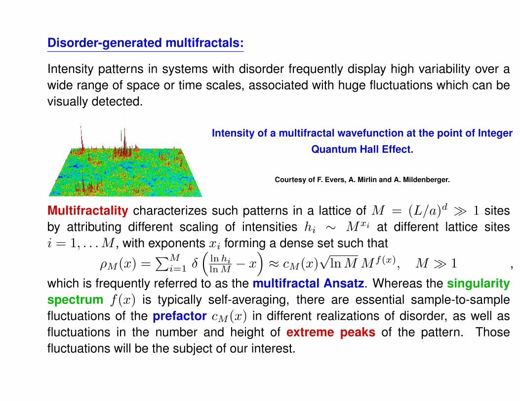
Intensity patterns in systems with disorder frequently display high variability over awide range of space or time scales, associated with huge fluctuations which can bevisually detected.

Intensity of a multifractal wavefunction at the point of IntegerQuantum Hall Effect.

Courtesy of F. Evers, A. Mirlin and A. Mildenberger.

Multifractality characterizes such patterns in a lattice of M = (L/a)d � 1 sitesby attributing different scaling of intensities hi ∼ Mxi at different lattice sitesi = 1, . . .M , with exponents xi forming a dense set such that

ρM(x) =∑Mi=1 δ

(lnhilnM − x

)≈ cM(x)

√lnMMf(x), M � 1 ,

which is frequently referred to as the multifractal Ansatz. Whereas the singularityspectrum f(x) is typically self-averaging, there are essential sample-to-samplefluctuations of the prefactor cM(x) in different realizations of disorder, as well asfluctuations in the number and height of extreme peaks of the pattern. Thosefluctuations will be the subject of our interest.

From disorder-generated multifractals to log-correlated fields:

Disorder-generated multifractal patterns of intensities h(r) are typically self-similar

E {hq(r1)hs(r2)} ∝(La

)yq,s (|r1−r2|a

)−zq,s, q, s ≥ 0, a� |r1 − r2| � L

and spatially homogeneous

E {hq(r1)} ∼ 1M

∑r h

q(r) ∝(La

)d(ζq−1)

where ζq and f(x) are related by the Legendre transform:

f ′(y∗) = −q and ζq = f(y∗) + q y∗.

The consistency of the two conditions for |r1 − r2| ∼ a and |r1 − r2| ∼ L implies:

yq,s = d(ζq+s − 1), zq,s = d(ζq+s − ζq − ζs + 1)

If we now introduce the field V (r) = lnh(r)− E {lnh(r)} and exploit the identitiesddsh

s|s=0 = lnh and ζ0 = 1 we arrive at the relation:

E {V (r1)V (r2)} = −g2 ln|r1−r2|L , g2 = d ∂2

∂s∂qζq+s|s=q=0

Conclusion: logarithm of a multifractal intensity is a log-correlated random field.To understand statistics of high values and extremes of general logarithmically correlatedrandom fields we consider the simplest 1D case of such process: the Gaussian 1/f noise.

Ideal Gaussian periodic 1/f noise:

We will mainly study an idealized periodic model for Gaussian 1/f noise defined as

V (t) =∑∞n=1

1√n

[vne

int + vne−int] , t ∈ [0, 2π)

where vn, vn are complex standard Gaussian i.i.d. with E{vnvn} = 1. It impliesthe formal covariance structure:

E {V (t1)V (t2)} = −2 ln |2 sin t1−t22 |, t1 6= t2

The corresponding process is a random distribution and in applications should beregularized. There are several alternative regularizations. E.g. one can replace thefunction V (t), t ∈ [0, 2π) with a sequence of M � 1 random mean-zero Gaussianvariables Vk ≡ V

(t = 2π

M k)

with the covariance matrix E {VkVm} given by

E {VkVm} = −2 ln |2 sin πM (k −m)|, Ckk = E

{V 2k

}> 2 lnM, ∀k = 1, . . . ,M

One also may give bona fide mathematical definition as e.g. 1D "projection" of the 2D Gaussian FreeField. We shall see that one may further consider aperiodic stationary logarithmically-correlated

processes as well as similar processes with stationary increments:

E {V (t1)V (t2)} ∝ − log |t1 − t2| or En

[V (t1)− V (t2)]2o∝ log |t1 − t2|

The multifractal intensity pattern is then generated by setting hi = eVi for eachi = 1, . . . ,M .

Ideal Gaussian periodic 1/f noise:

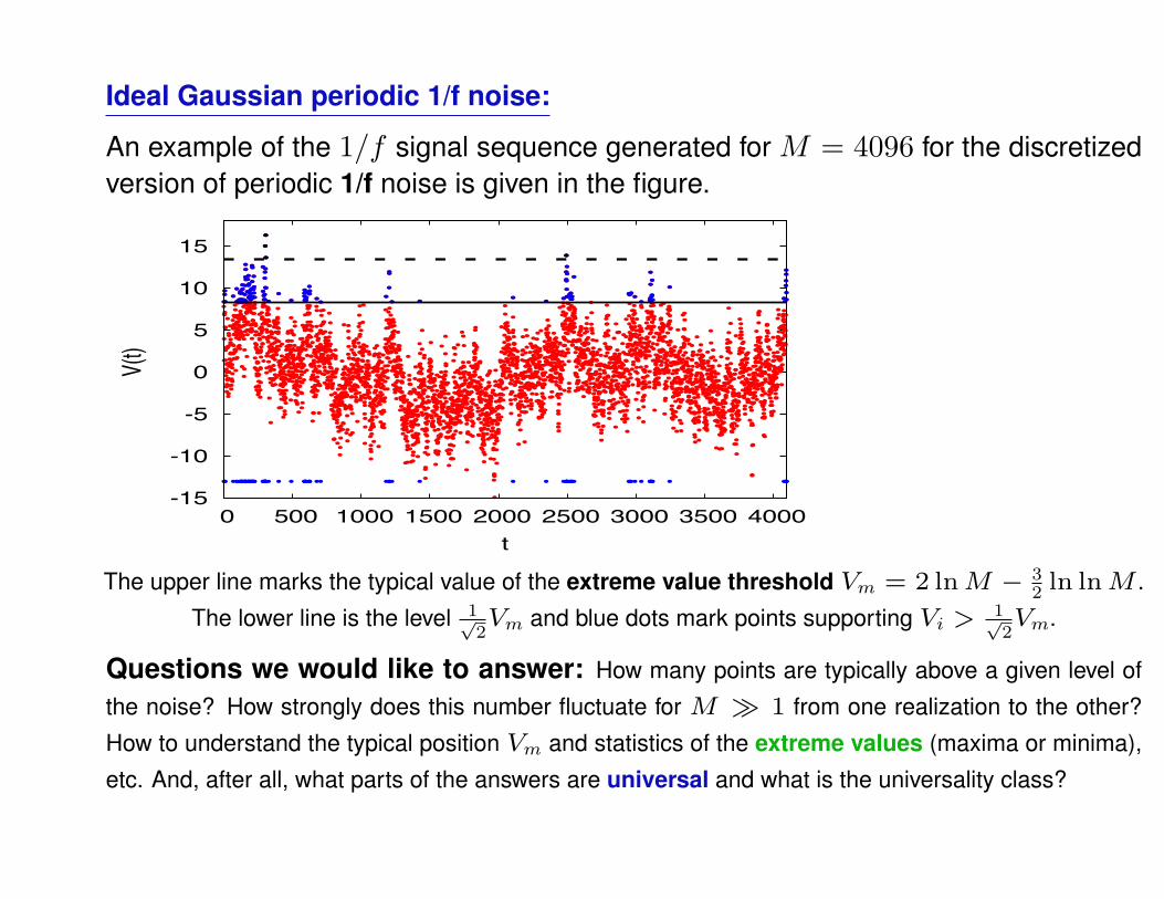
An example of the 1/f signal sequence generated for M = 4096 for the discretizedversion of periodic 1/f noise is given in the figure.

-15

-10

-5

0

5

10

15

0 500 1000 1500 2000 2500 3000 3500 4000

V(t)

t

The upper line marks the typical value of the extreme value threshold Vm = 2 lnM − 32 ln lnM .

The lower line is the level 1√2Vm and blue dots mark points supporting Vi > 1√

2Vm.

Questions we would like to answer: How many points are typically above a given level of

the noise? How strongly does this number fluctuate for M � 1 from one realization to the other?

How to understand the typical position Vm and statistics of the extreme values (maxima or minima),

etc. And, after all, what parts of the answers are universal and what is the universality class?

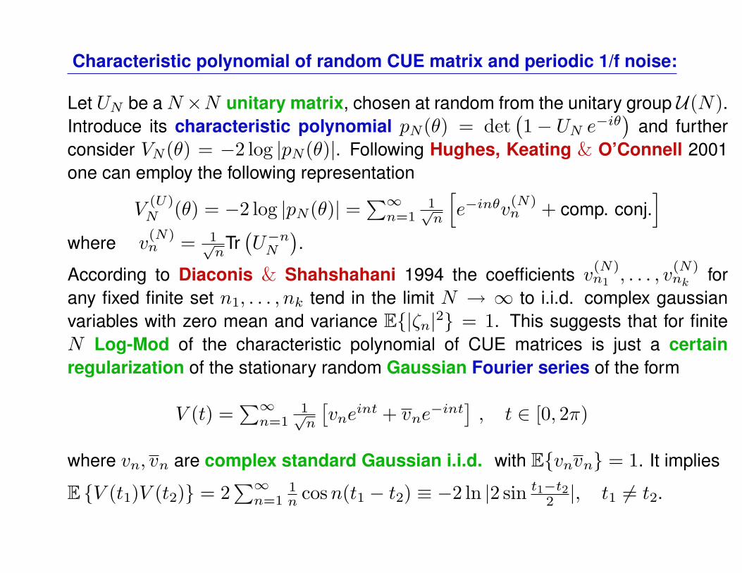
Characteristic polynomial of random CUE matrix and periodic 1/f noise:

Let UN be aN×N unitary matrix, chosen at random from the unitary group U(N).Introduce its characteristic polynomial pN(θ) = det

(1− UN e−iθ

)and further

consider VN(θ) = −2 log |pN(θ)|. Following Hughes, Keating & O’Connell 2001one can employ the following representation

V(U)N (θ) = −2 log |pN(θ)| =

∑∞n=1

1√n

[e−inθv

(N)n + comp. conj.

]where v

(N)n = 1√

nTr(U−nN

).

According to Diaconis & Shahshahani 1994 the coefficients v(N)n1 , . . . , v

(N)nk for

any fixed finite set n1, . . . , nk tend in the limit N → ∞ to i.i.d. complex gaussianvariables with zero mean and variance E{|ζn|2} = 1. This suggests that for finiteN Log-Mod of the characteristic polynomial of CUE matrices is just a certainregularization of the stationary random Gaussian Fourier series of the form

V (t) =∑∞n=1

1√n

[vne

int + vne−int] , t ∈ [0, 2π)

where vn, vn are complex standard Gaussian i.i.d. with E{vnvn} = 1. It implies

E {V (t1)V (t2)} = 2∑∞n=1

1n cosn(t1 − t2) ≡ −2 ln |2 sin t1−t2

2 |, t1 6= t2.

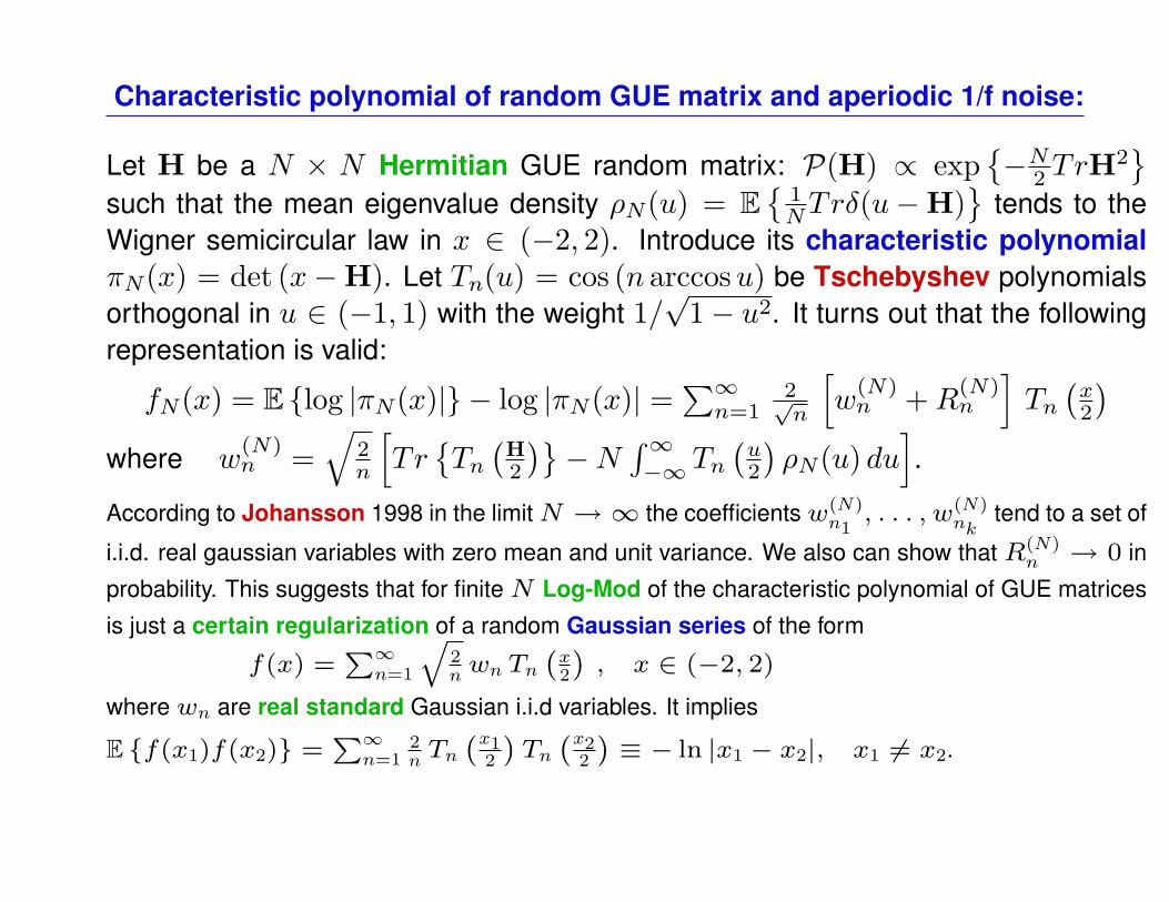
Characteristic polynomial of random GUE matrix and aperiodic 1/f noise:

Let H be a N × N Hermitian GUE random matrix: P(H) ∝ exp{−N2 TrH

2}

such that the mean eigenvalue density ρN(u) = E{

1NTrδ(u−H)

}tends to the

Wigner semicircular law in x ∈ (−2, 2). Introduce its characteristic polynomialπN(x) = det (x−H). Let Tn(u) = cos (n arccosu) be Tschebyshev polynomialsorthogonal in u ∈ (−1, 1) with the weight 1/

√1− u2. It turns out that the following

representation is valid:

fN(x) = E {log |πN(x)|} − log |πN(x)| =∑∞n=1

2√n

[w

(N)n +R

(N)n

]Tn(x2

)where w

(N)n =

√2n

[Tr{Tn(H2

)}−N

∫∞−∞ Tn

(u2

)ρN(u) du

].

According to Johansson 1998 in the limitN →∞ the coefficientsw(N)n1, . . . , w(N)

nktend to a set of

i.i.d. real gaussian variables with zero mean and unit variance. We also can show that R(N)n → 0 in

probability. This suggests that for finiteN Log-Mod of the characteristic polynomial of GUE matrices

is just a certain regularization of a random Gaussian series of the form

f(x) =P∞

n=1

q2n wn Tn

`x2

´, x ∈ (−2, 2)

where wn are real standard Gaussian i.i.d variables. It implies

E {f(x1)f(x2)} =P∞

n=12n Tn

`x12

´Tn`x2

2

´≡ − ln |x1 − x2|, x1 6= x2.

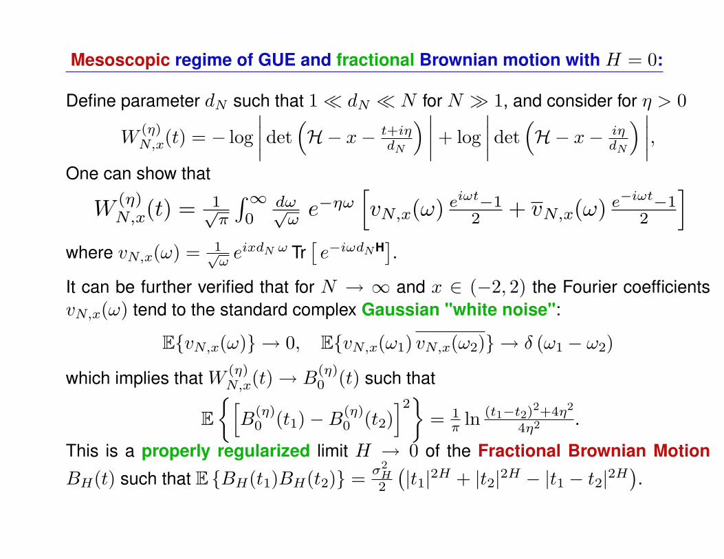
Mesoscopic regime of GUE and fractional Brownian motion with H = 0:

Define parameter dN such that 1� dN � N for N � 1, and consider for η > 0

W(η)N,x(t) = − log

∣∣∣∣ det(H− x− t+iη

dN

) ∣∣∣∣+ log∣∣∣∣ det

(H− x− iη

dN

) ∣∣∣∣,One can show that

W(η)N,x(t) = 1√

π

∫∞0

dω√ωe−ηω

[vN,x(ω) e

iωt−12 + vN,x(ω) e

−iωt−12

]where vN,x(ω) = 1√

ωeixdN ω Tr

[e−iωdNH

].

It can be further verified that for N → ∞ and x ∈ (−2, 2) the Fourier coefficientsvN,x(ω) tend to the standard complex Gaussian "white noise":

E{vN,x(ω)} → 0, E{vN,x(ω1) vN,x(ω2)} → δ (ω1 − ω2)

which implies that W (η)N,x(t)→ B

(η)0 (t) such that

E{[B

(η)0 (t1)−B(η)

0 (t2)]2}

= 1π ln (t1−t2)2+4η2

4η2 .

This is a properly regularized limit H → 0 of the Fractional Brownian Motion

BH(t) such that E {BH(t1)BH(t2)} = σ2H2

(|t1|2H + |t2|2H − |t1 − t2|2H

).

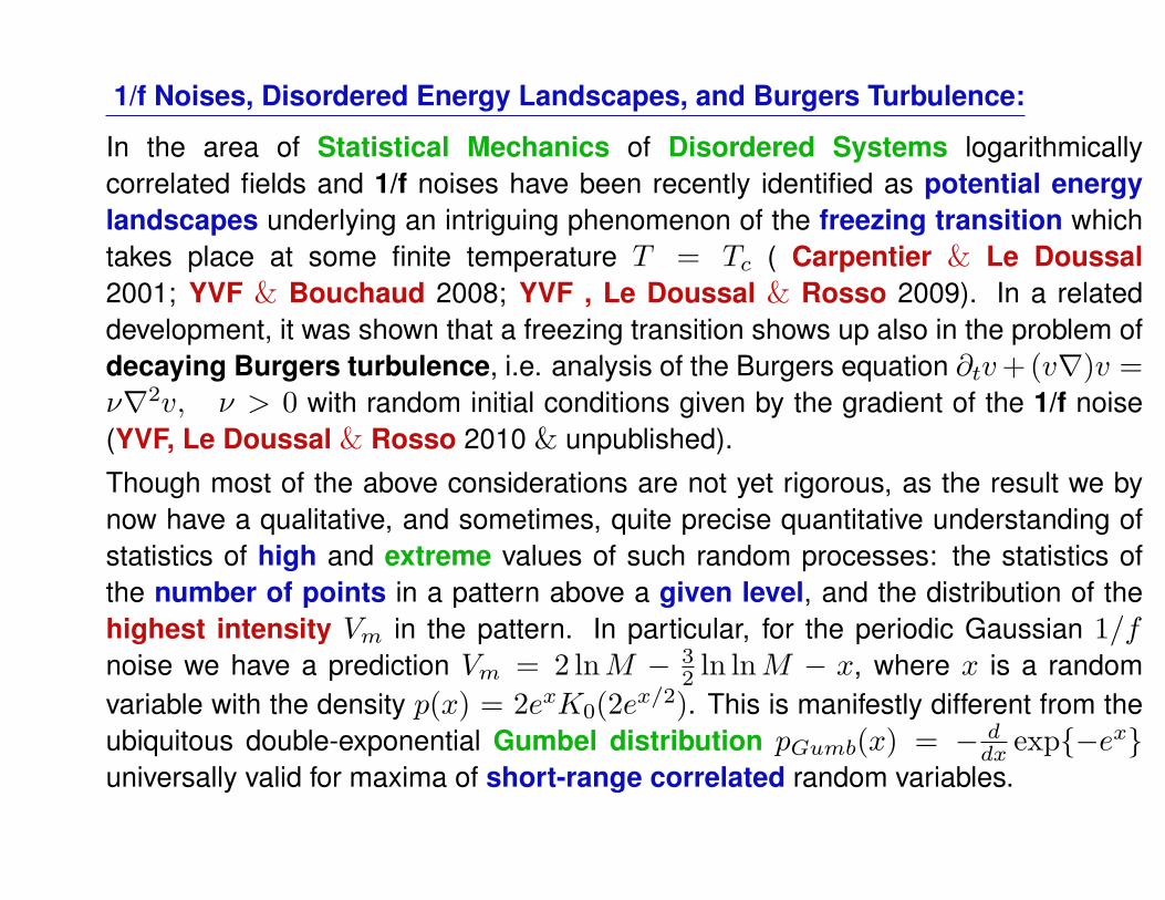
1/f Noises, Disordered Energy Landscapes, and Burgers Turbulence:

In the area of Statistical Mechanics of Disordered Systems logarithmicallycorrelated fields and 1/f noises have been recently identified as potential energylandscapes underlying an intriguing phenomenon of the freezing transition whichtakes place at some finite temperature T = Tc ( Carpentier & Le Doussal2001; YVF & Bouchaud 2008; YVF , Le Doussal & Rosso 2009). In a relateddevelopment, it was shown that a freezing transition shows up also in the problem ofdecaying Burgers turbulence, i.e. analysis of the Burgers equation ∂tv+(v∇)v =ν∇2v, ν > 0 with random initial conditions given by the gradient of the 1/f noise(YVF, Le Doussal & Rosso 2010 & unpublished).

Though most of the above considerations are not yet rigorous, as the result we bynow have a qualitative, and sometimes, quite precise quantitative understanding ofstatistics of high and extreme values of such random processes: the statistics ofthe number of points in a pattern above a given level, and the distribution of thehighest intensity Vm in the pattern. In particular, for the periodic Gaussian 1/fnoise we have a prediction Vm = 2 lnM − 3

2 ln lnM − x, where x is a randomvariable with the density p(x) = 2exK0(2ex/2). This is manifestly different from theubiquitous double-exponential Gumbel distribution pGumb(x) = − d

dx exp{−ex}universally valid for maxima of short-range correlated random variables.

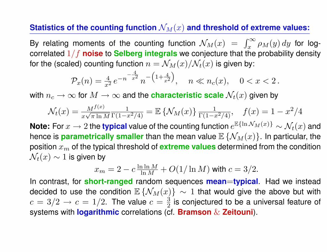
Statistics of the counting function NM(x) and threshold of extreme values:

By relating moments of the counting function NM(x) =∫∞xρM(y) dy for log-

correlated 1/f noise to Selberg integrals we conjecture that the probability densityfor the (scaled) counting function n = NM(x)/Nt(x) is given by:

Px(n) = 4x2 e−n− 4x2n−“

1+ 4x2

”, n� nc(x), 0 < x < 2 .

with nc →∞ for M →∞ and the characteristic scale Nt(x) given by

Nt(x) = Mf(x)

x√π lnM

1Γ(1−x2/4)

= E {NM(x)} 1Γ(1−x2/4)

, f(x) = 1− x2/4

Note: For x→ 2 the typical value of the counting function eE{lnNM(x)} ∼ Nt(x) andhence is parametrically smaller than the mean value E {NM(x)}. In particular, theposition xm of the typical threshold of extreme values determined from the conditionNt(x) ∼ 1 is given by

xm = 2− c ln lnMlnM +O(1/ lnM) with c = 3/2.

In contrast, for short-ranged random sequences mean=typical. Had we insteaddecided to use the condition E {NM(x)} ∼ 1 that would give the above but withc = 3/2 → c = 1/2. The value c = 3

2 is conjectured to be a universal feature ofsystems with logarithmic correlations (cf. Bramson & Zeitouni).

Threshold of extreme values for self-similar multifractal fields:Apart from 1/f noise and its incarnations (like modulus of characteristic polynomials of randommatrices) the new universality class is believed to include: the 2D Gaussian free field,branching random walks & polymers on disordered trees, modulus of zeta-function alongthe critical line, fluctuations of shapes of random Young tableaux sampled with Plancherelmeasure, some models in turbulence and financial mathematics and, with due modificationsthe disorder-generated multifractals.

Namely, consider a multifractal random probability measure pi ∼ M−αi, i =1, . . . ,M such that

∑Mi=1 pi = 1 characterized by a general non-parabolic

singularity spectrum f(α) with the left endpoint at α = α− > 0. Then very similarconsideration based on insights from Mirlin & Evers 2000 suggests that the extremevalue threshold should be given by pm = M−αm, where αm

αm ≈ α− + 32

1f ′(α−)

ln lnMlnM ⇒ − ln pm ≈ α− lnM + 3

21

f ′(α−) ln lnMFor branching random walks this is indeed rigorously proved: L. Addario-Berry & B. Reed2009; E. Aidekon 2012Work in progress: testing such a prediction for multifractal eigenvectors of a certain N × Nrandom matrix ensemble introduced by E. Bogomolny & O. Giraud, Phys. Rev. Lett. 106 044101(2011). Preliminary numerics is supportive of the theory.

Distribution of the absolute maximum: partition function approach:

Given the sequence{Vi, i = 1, . . . ,M} we are interested in finding the distributionof V(m) = max(V1, . . . , VM) that is

P (v) = Prob(V(m) < v) = Prob(Vi < v, ∀i) = E{∏M

i=1 θ(v − Vi)}

Next we use: limq→∞ exp[−e−q(v−Vi)

]={

1 v > Vi0 v < Vi

≡ θ(v − Vi)

which immediately shows that:

P (v) = Prob(V(m) < v) = limq→∞E {exp [−e−qvZq]} , where Zq =∑i=1 e

qVi

In the limit lnM � 1 moments of Zq for |q| < 1 can be again related to Selberg integrals,which allows to extract the function Gq(v) = E

˘exp

ˆ−e−qvZq

˜¯for q < 1:

Gq(v) = gq (v − cq lnM) where cq =“q + 1

q

”and gq(v) =

R∞0dt exp

n−t− e−qvt−q

2o

One may further notice that not only cq = cq−1 but the whole function satisfies a quiteremarkable duality relation

gq(v) = 1 +P∞

n=1(−1)n

n!

he−nqvΓ(1− nq2) + e−n

vqΓ“

1− nq2

”i= g1

q(x)

THIS HOWEVER STILL DOES NOT ALLOW TO CONTINUE TO q > 1!

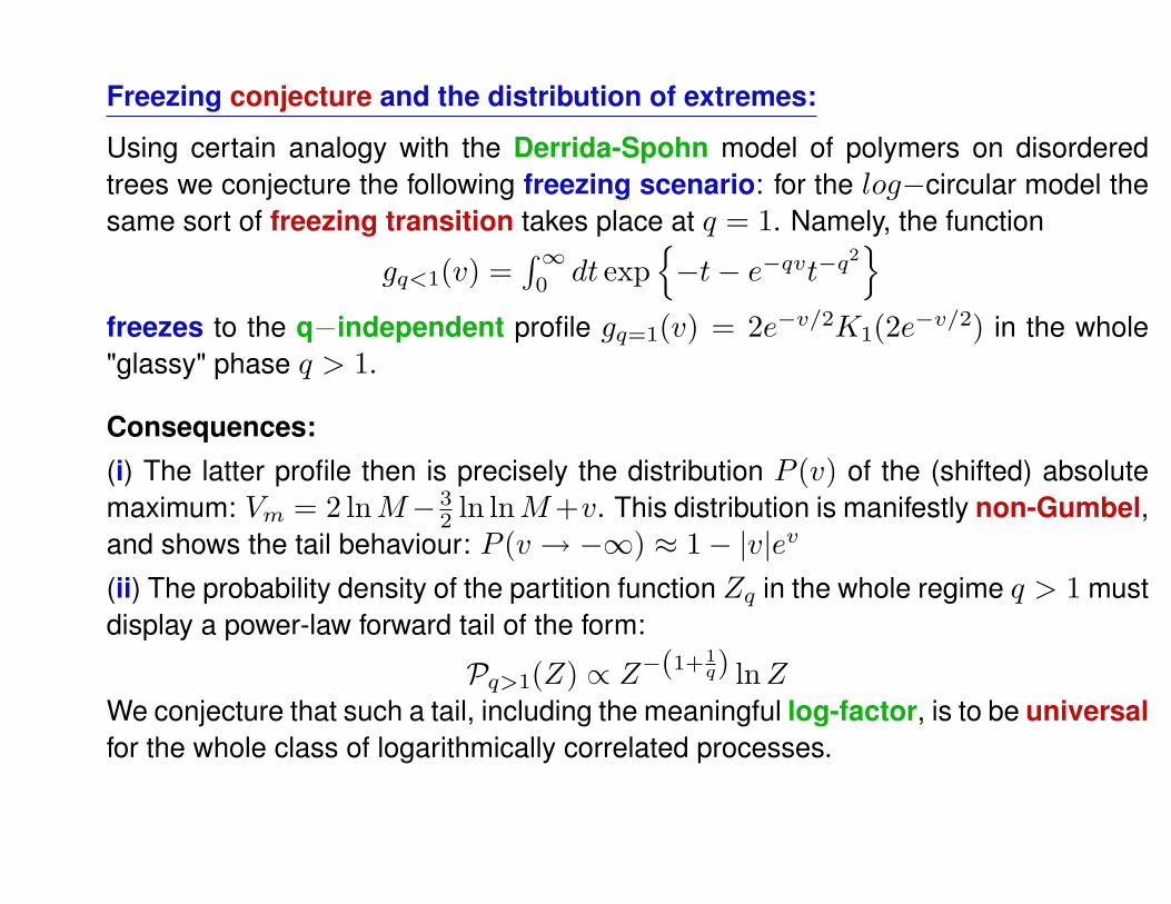
Freezing conjecture and the distribution of extremes:

Using certain analogy with the Derrida-Spohn model of polymers on disorderedtrees we conjecture the following freezing scenario: for the log−circular model thesame sort of freezing transition takes place at q = 1. Namely, the function

gq<1(v) =∫∞

0dt exp

{−t− e−qvt−q2

}freezes to the q−independent profile gq=1(v) = 2e−v/2K1(2e−v/2) in the whole"glassy" phase q > 1.

Consequences:(i) The latter profile then is precisely the distribution P (v) of the (shifted) absolutemaximum: Vm = 2 lnM− 3

2 ln lnM+v. This distribution is manifestly non-Gumbel,and shows the tail behaviour: P (v → −∞) ≈ 1− |v|ev

(ii) The probability density of the partition function Zq in the whole regime q > 1 mustdisplay a power-law forward tail of the form:

Pq>1(Z) ∝ Z−(1+1q) lnZ

We conjecture that such a tail, including the meaningful log-factor, is to be universalfor the whole class of logarithmically correlated processes.

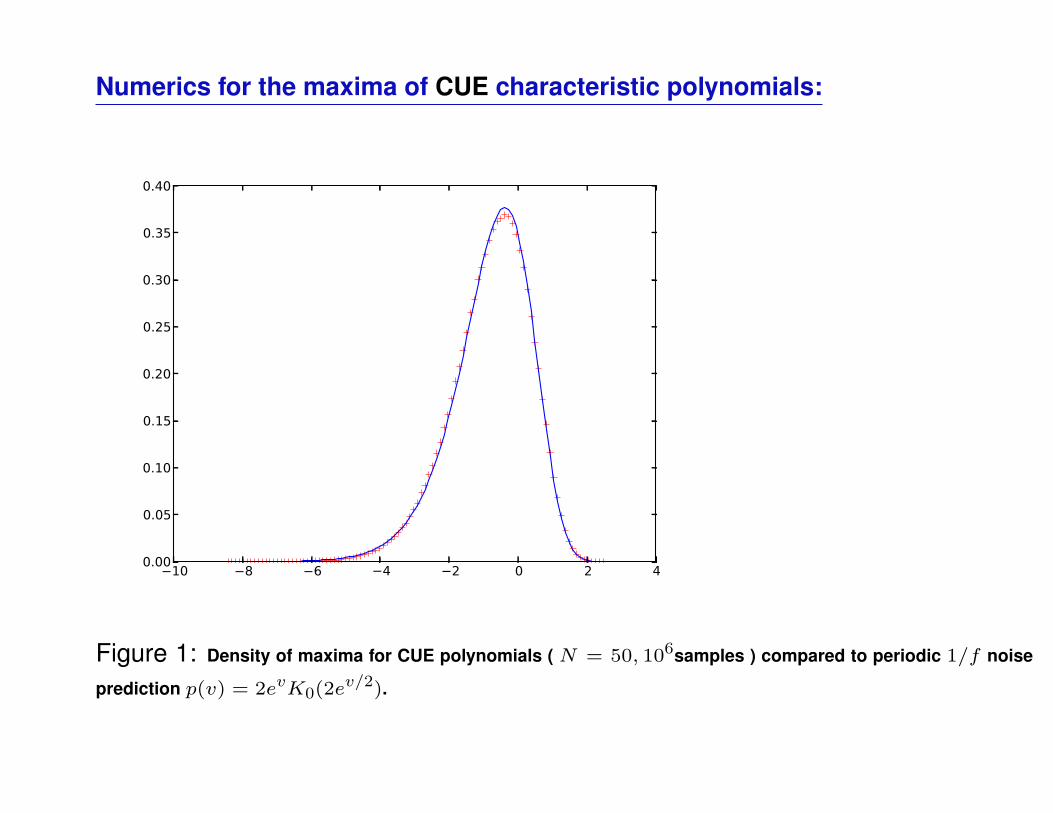
Numerics for the maxima of CUE characteristic polynomials:

Figure 1: Density of maxima for CUE polynomials ( N = 50, 106samples ) compared to periodic 1/f noise

prediction p(v) = 2evK0(2ev/2).

From 1/f noise to Riemann ζ(1/2 + it):

As is well-known, zeroes of the Riemann zeta-function ζ(s) along the "critical line"s = 1/2 + it, t ∈ R behave statistically as a sequence of eigenvalues of randomHermitian GUE matrices (Montgomery 1983). Following the ideas of Keating &Snaith 2000 one can expect that log-mod of the Riemann zeta-function ζ(1/2 + it)locally resembles log-mod of CUE characteristic polynomial, and hence a (non-periodic) version of the 1/f noise, see also P. Bourgade 2010. One can exploit thisfact to predict statistics of moments and high values of the Riemann zeta along thecritical line using the previously exposed ideas (YVF, Keating 2012).

Our approach to statistics of ζ(1/2 + it):

We expect a single unitary matrix of size NT = log (T/2π) � 1 to model theRiemann zeta ζ(1/2 + it), statistically, over a range of T ≤ t ≤ T + 2π. We thussuggest splitting the critical line into ranges of length 2π, and making the statisticsof ζ(1/2 + it) over the many ranges.

There are roughly NT zeros in each range of length 2π. At heights T ∼ 1022− 1028

we used samples that spans ≈ 107 zeros.

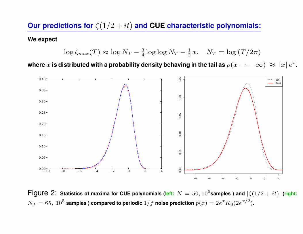
Our predictions for ζ(1/2 + it) and CUE characteristic polynomials:

We expect

log ζmax(T ) ≈ logNT − 34 log logNT − 1

2 x, NT = log (T/2π)

where x is distributed with a probability density behaving in the tail as ρ(x→ −∞) ≈ |x| ex.

−8 −6 −4 −2 0 2 40.

000.

050.

100.

150.

200.

25 p(x)data

Figure 2: Statistics of maxima for CUE polynomials (left: N = 50, 106samples ) and |ζ(1/2 + it)| (right:

NT = 65, 105 samples ) compared to periodic 1/f noise prediction p(x) = 2exK0(2ex/2).

Summary:

I. Disorder-generated multifractal patterns are intimately connected to log-correlated random fields.II. log-mod of characteristic polynomials of random matrices on the global scaleare examples of log-correlated Gaussian 1/f noises. The same objects onmesoscopic scale are examples of Fractional Brownian Motion with H = 0.III. Exploiting the methods of statistical mechanics of disordered systemswe attempted to understand the statistics of minima/maxima of the CUEcharacteristic polynomial over various intervals, as well as the relatedmoments and high values.IV. The above picture can be translated into making non-trivial conjecturesabout statistics of moments and high values of (i) the Riemann zeta along thecritical line (ii) a more general class of disorder-generated multifractal fields.