dispersal ability and habitat requirements determine...

Dispersal ability and habitat requirements determinelandscape-level genetic patterns in desert aquatic insects

IVAN C. PHILLIPSEN,* EMILY H. KIRK,* MICHAEL T. BOGAN,* MERYL C. MIMS,† JULIAN D.

OLDEN† and DAVID A. LYTLE*

*Department of Integrative Biology, Oregon State University, 3029 Cordley Hall, Corvallis, OR 97331, USA, †School of Aquatic

and Fishery Sciences, University of Washington, 1122 NE Boat Street, Seattle, WA 98195, USA

Abstract

Species occupying the same geographic range can exhibit remarkably different popula-

tion structures across the landscape, ranging from highly diversified to panmictic.

Given limitations on collecting population-level data for large numbers of species,

ecologists seek to identify proximate organismal traits—such as dispersal ability, habi-

tat preference and life history—that are strong predictors of realized population struc-

ture. We examined how dispersal ability and habitat structure affect the regional

balance of gene flow and genetic drift within three aquatic insects that represent the

range of dispersal abilities and habitat requirements observed in desert stream insect

communities. For each species, we tested for linear relationships between genetic dis-

tances and geographic distances using Euclidean and landscape-based metrics of resis-

tance. We found that the moderate-disperser Mesocapnia arizonensis (Plecoptera:

Capniidae) has a strong isolation-by-distance pattern, suggesting migration–drift equi-librium. By contrast, population structure in the flightless Abedus herberti (Hemiptera:

Belostomatidae) is influenced by genetic drift, while gene flow is the dominant force

in the strong-flying Boreonectes aequinoctialis (Coleoptera: Dytiscidae). The best-fitting

landscape model for M. arizonensis was based on Euclidean distance. Analyses also

identified a strong spatial scale-dependence, where landscape genetic methods only

performed well for species that were intermediate in dispersal ability. Our results

highlight the fact that when either gene flow or genetic drift dominates in shaping

population structure, no detectable relationship between genetic and geographic dis-

tances is expected at certain spatial scales. This study provides insight into how gene

flow and drift interact at the regional scale for these insects as well as the organisms

that share similar habitats and dispersal abilities.

Keywords: aquatic insects, freshwater, gene flow, isolation by distance, landscape genetics

Received 24 June 2014; revision received 17 October 2014; accepted 26 October 2014

Introduction

The relationship between physical landscape structure

and the population dynamics of individual species is

often complex. Organisms that occupy nearly identical

geographic ranges may exhibit radically different popu-

lation structures, and these differences will depend on

the biological attributes of each species: their dispersal

abilities, habitat requirements, life histories, and other

factors. In particular, dispersal ability and habitat

requirements are expected to have strong influences on

gene flow, genetic drift and other population-level pro-

cess. Dispersal (which facilitates gene flow) between

populations can be limited for species with strict habitat

requirements, especially when that habitat is frag-

mented or rare in the landscape (Bonte et al. 2003), but

such limitations can be overcome by species with strong

dispersal abilities. Landscape features representing criti-

cal habitat requirements can interact with dispersalCorrespondence: Ivan C. Phillipsen, Fax: 541 737 0501;

E-mail: [email protected]

© 2014 John Wiley & Sons Ltd

Molecular Ecology (2015) 24, 54–69 doi: 10.1111/mec.13003

ability to either inhibit or facilitate the movement of

individuals between habitat patches (Manel et al. 2003).

Similarly, the mode of dispersal may determine how

different species respond to the same landscape features

(Goldberg & Waits 2010).

For the long-term conservation management of spe-

cies in the wild, it is essential to understand how pro-

cesses such as gene flow and genetic drift affect genetic

diversity within each species of concern (Toro & Cabal-

lero 2005; Allendorf et al. 2012), yet it is intractable to

collect population-level data on every species in the

landscape. Thus, an important goal of population genet-

ics is to find general relationships between organisms

with particular biological attributes (dispersal ability,

habitat requirements, life history) and their population

genetic structures across the landscape. Such informa-

tion is especially needed in the context of climate

change, where shifting habitat distributions are likely to

affect rates of gene flow among populations as well as

individual population sizes (Rice & Emery 2003).

Differences in dispersal ability and habitat require-

ments can lead to demographic processes that favour

strong isolation of populations, step-wise connectivity

across the landscape or panmixia. Genetic differentia-

tion between a pair of populations or among a set of

populations reaches an equilibrium level when the

homogenizing effect of gene flow is balanced by the dif-

ferentiation that occurs due to genetic drift (for neutral

loci when mutation is negligible). The stochastic evolu-

tionary force of genetic drift occurs within each popula-

tion and is a function of effective population size (Ne;

Nei & Tajima 1981). Hutchison & Templeton (1999),

building on Slatkin (1993), presented a framework to

describe the relationship between pairwise genetic dis-

tance and geographic (Euclidean) distance that would

arise under conditions of regional equilibrium as well

as several forms of disequilibrium. Under equilibrium

conditions, the line-of-best-fit will have an intercept

near zero and a significant, positive slope (Type B in

Fig. 1). Variance in genetic distance will increase with

geographic distance in this case, such that there is more

scatter in the y-axis at greater geographic distances.

This is the pattern produced at equilibrium under an

isolation-by-distance (IBD) process, when gene flow fol-

lows a stepping-stone model (Mal�ecot 1955; Kimura &

Weiss 1964). This IBD pattern will not be observed

when either gene flow or genetic drift is more influen-

tial. In the situation where one of these forces over-

whelms, the other we expect a flat line-of-best-fit (i.e. a

nonsignificant slope). When gene flow is minimal and

populations are diverging randomly due to drift,

genetic distances are expected to be large at all spatial

Geographic distanceGeographic distanceGeographic distance

Gen

etic

dis

tanc

e

Moderate dispersalLow dispersal High dispersal

TYPE

ATYPE

BTYPE

C

Fig. 1 Predicted relationships between genetic distances and geographic (Euclidean) distances between pairs of populations. The

black line is the regression line, and the shaded area shows the spread (i.e. variance) in the pairwise genetic distances across the geo-

graphic distances. When genetic drift is more influential than gene flow (Type A), as is predicted for species with low dispersal, the

slope of the line should not differ significantly from zero, the intercept will be high, and the variance will be high across all geo-

graphic distances. For species with moderate dispersal, a positive slope is predicted (Type B). The intercept should be near zero, and

variance should increase with increasing geographic distance. Gene flow should be more influential than drift for species with high

dispersal (Type C). The regression line in this case should not significantly deviate from zero, the intercept should be small, and vari-

ance is low across all geographic distances.


POPULATION GENETICS OF DESERT AQUATIC INSECTS 55

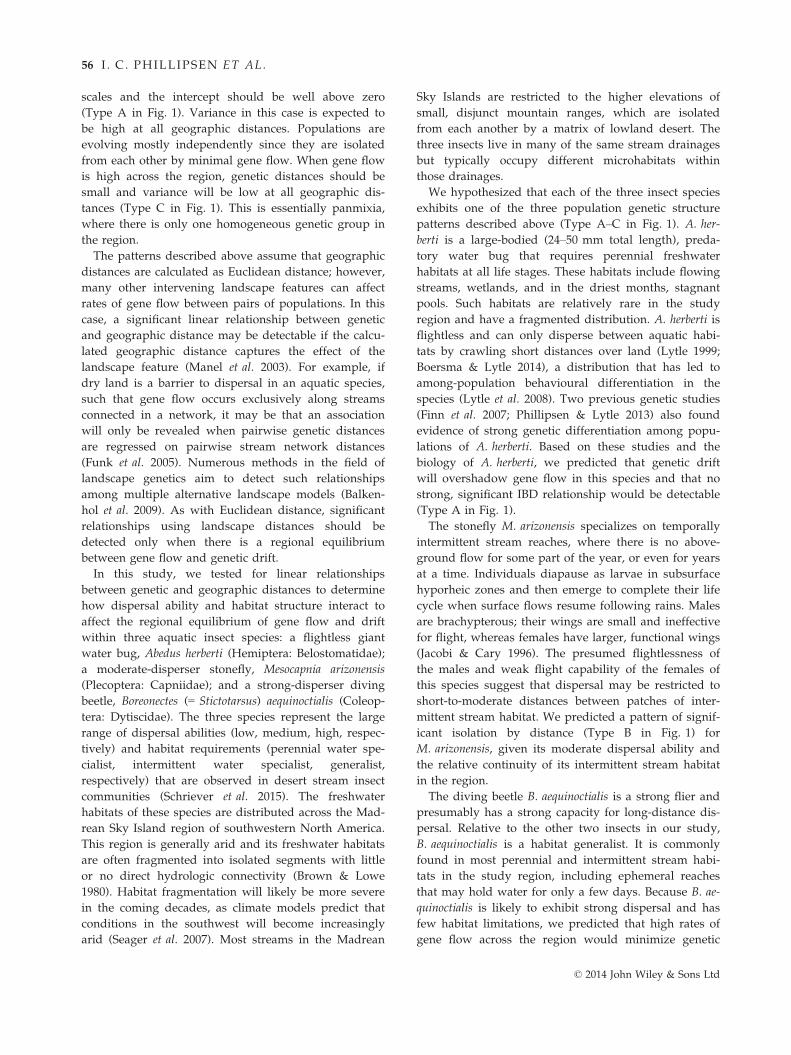
scales and the intercept should be well above zero

(Type A in Fig. 1). Variance in this case is expected to

be high at all geographic distances. Populations are

evolving mostly independently since they are isolated

from each other by minimal gene flow. When gene flow

is high across the region, genetic distances should be

small and variance will be low at all geographic dis-

tances (Type C in Fig. 1). This is essentially panmixia,

where there is only one homogeneous genetic group in

the region.

The patterns described above assume that geographic

distances are calculated as Euclidean distance; however,

many other intervening landscape features can affect

rates of gene flow between pairs of populations. In this

case, a significant linear relationship between genetic

and geographic distance may be detectable if the calcu-

lated geographic distance captures the effect of the

landscape feature (Manel et al. 2003). For example, if

dry land is a barrier to dispersal in an aquatic species,

such that gene flow occurs exclusively along streams

connected in a network, it may be that an association

will only be revealed when pairwise genetic distances

are regressed on pairwise stream network distances

(Funk et al. 2005). Numerous methods in the field of

landscape genetics aim to detect such relationships

among multiple alternative landscape models (Balken-

hol et al. 2009). As with Euclidean distance, significant

relationships using landscape distances should be

detected only when there is a regional equilibrium

between gene flow and genetic drift.

In this study, we tested for linear relationships

between genetic and geographic distances to determine

how dispersal ability and habitat structure interact to

affect the regional equilibrium of gene flow and drift

within three aquatic insect species: a flightless giant

water bug, Abedus herberti (Hemiptera: Belostomatidae);

a moderate-disperser stonefly, Mesocapnia arizonensis

(Plecoptera: Capniidae); and a strong-disperser diving

beetle, Boreonectes (= Stictotarsus) aequinoctialis (Coleop-

tera: Dytiscidae). The three species represent the large

range of dispersal abilities (low, medium, high, respec-

tively) and habitat requirements (perennial water spe-

cialist, intermittent water specialist, generalist,

respectively) that are observed in desert stream insect

communities (Schriever et al. 2015). The freshwater

habitats of these species are distributed across the Mad-

rean Sky Island region of southwestern North America.

This region is generally arid and its freshwater habitats

are often fragmented into isolated segments with little

or no direct hydrologic connectivity (Brown & Lowe

1980). Habitat fragmentation will likely be more severe

in the coming decades, as climate models predict that

conditions in the southwest will become increasingly

arid (Seager et al. 2007). Most streams in the Madrean

Sky Islands are restricted to the higher elevations of

small, disjunct mountain ranges, which are isolated

from each another by a matrix of lowland desert. The

three insects live in many of the same stream drainages

but typically occupy different microhabitats within

those drainages.

We hypothesized that each of the three insect species

exhibits one of the three population genetic structure

patterns described above (Type A–C in Fig. 1). A. her-

berti is a large-bodied (24–50 mm total length), preda-

tory water bug that requires perennial freshwater

habitats at all life stages. These habitats include flowing

streams, wetlands, and in the driest months, stagnant

pools. Such habitats are relatively rare in the study

region and have a fragmented distribution. A. herberti is

flightless and can only disperse between aquatic habi-

tats by crawling short distances over land (Lytle 1999;

Boersma & Lytle 2014), a distribution that has led to

among-population behavioural differentiation in the

species (Lytle et al. 2008). Two previous genetic studies

(Finn et al. 2007; Phillipsen & Lytle 2013) also found

evidence of strong genetic differentiation among popu-

lations of A. herberti. Based on these studies and the

biology of A. herberti, we predicted that genetic drift

will overshadow gene flow in this species and that no

strong, significant IBD relationship would be detectable

(Type A in Fig. 1).

The stonefly M. arizonensis specializes on temporally

intermittent stream reaches, where there is no above-

ground flow for some part of the year, or even for years

at a time. Individuals diapause as larvae in subsurface

hyporheic zones and then emerge to complete their life

cycle when surface flows resume following rains. Males

are brachypterous; their wings are small and ineffective

for flight, whereas females have larger, functional wings

(Jacobi & Cary 1996). The presumed flightlessness of

the males and weak flight capability of the females of

this species suggest that dispersal may be restricted to

short-to-moderate distances between patches of inter-

mittent stream habitat. We predicted a pattern of signif-

icant isolation by distance (Type B in Fig. 1) for

M. arizonensis, given its moderate dispersal ability and

the relative continuity of its intermittent stream habitat

in the region.

The diving beetle B. aequinoctialis is a strong flier and

presumably has a strong capacity for long-distance dis-

persal. Relative to the other two insects in our study,

B. aequinoctialis is a habitat generalist. It is commonly

found in most perennial and intermittent stream habi-

tats in the study region, including ephemeral reaches

that may hold water for only a few days. Because B. ae-

quinoctialis is likely to exhibit strong dispersal and has

few habitat limitations, we predicted that high rates of

gene flow across the region would minimize genetic


56 I . C . PHILLIPSEN ET AL.

distances for this species and that we would not detect

a significant IBD pattern (Type C in Fig. 1).

For each species, we tested for linear relationships

between genetic distances and geographic distances

using Euclidean distance for the latter as well as land-

scape-based distances that reflect alternative hypotheses

describing the permeability of the landscape for each of

the insect species. We developed and evaluated land-

scape genetics models to determine which, if any, of the

landscape features have an important influence on pop-

ulation structure. We were particularly interested in

any effects of hydrological connectivity on genetic dis-

tance, since these species occupy stream habitats in an

arid environment.

Methods

Data collection

Insects samples were collected in southeastern Arizona

(USA) between 2010 and 2012 (Fig. 2; Table 1). Most of

the A. herberti samples were collected earlier, between

2002 and 2010 (Phillipsen & Lytle 2013). Whole adult

specimens (and some larval specimens for A. herberti

and M. arizonensis in a few localities) were sampled and

preserved in 95% ethanol. Sampling for the three spe-

cies was conducted at the same approximate spatial

extent within the 25 000 km2 study region (Fig. 2). Sam-

ple sizes ranged from 9 to 94 (median = 28) individuals

per population for A. herberti, 10–42 (median = 30) for

M. arizonensis and 9–55 (median = 30) for B. aequinocti-

alis (Table 1).

Genomic DNA for B. aequinoctialis, M. arizonensis and

some A. herberti populations was extracted from tissue

of each specimen using DNeasy Blood and Tissue Kits

(QIAGEN). Multilocus microsatellite genotypes were

generated for each individual using the protocols in

Phillipsen & Lytle (2013), which was also the source of

most of the A. herberti genotype data. Most of the data

for A. herberti used in the present study were previously

analysed by Phillipsen & Lytle (2013). A pilot analysis

was used to identify useful microsatellite loci from a

candidate set of >100 loci, based on sufficient among-

population variability and conformity to Hardy–Wein-

berg equilibrium. Final numbers of microsatellite loci

used per species were as follows: 10 for A. herberti

(Daly-Engel et al. 2012), 11 for M. arizonensis and 8 for

B. aequinoctialis. Information on the loci for the latter

two species is provided in Appendix I. Loci were multi-

plexed for amplification via polymerase chain reaction

(PCR) using Multiplex PCR kits (QIAGEN). Amplified

PCR products were run on an ABI 3730 sequencer, and

individuals were genotyped using the GENEMAPPER 4.1

software (Applied Biosystems).

Fig. 2 Map of the study region in southeastern Arizona, USA,

showing the distribution of sampling localities for the three

insect species. The inset in the top panel shows location of the

study region. The three major genetic groups identified in the

STRUCTURE analysis for Mesocapnia arizonensis are shown in the

middle panel. Two major groups were identified for Abedus her-

berti (top panel) in a previous study (Phillipsen & Lytle 2013).

Our samples of Boreonectes aequinoctialis (bottom panel) were

found to belong to a single group in the STRUCTURE analysis.



Table 1 Population sampling localities, sample sizes (n), geographic coordinates (UTM E and UTM N) and population metrics for

Abedus herberti, Mesocapnia arizonensis and Boreonectes aequinoctialis in southeastern Arizona, USA

Species Locality n Lat Lon AR Ho He FIS Ne

A. herberti 1 13 31.4996 �110.4094 3.56 0.52 0.55 0.07 �530 (15–∞)2 31 31.5187 �110.3875 4.52 0.57 0.68 0.17* �1854 (87–∞)3 94 31.4732 �110.3511 4.38 0.59 0.68 0.14* 96 (51–334)4 63 31.4410 �110.3180 4.13 0.52 0.62 0.15* 669 (142–∞)5 38 31.7882 �110.6376 3.64 0.46 0.62 0.26* 3 (1–∞)6 25 31.8630 �110.5727 4.67 0.54 0.71 0.24* 20 (11–61)

7 20 31.6518 �110.7045 3.64 0.48 0.56 0.14 25 (16–50)8 18 31.8104 �110.3943 3.89 0.46 0.64 0.30* 19 (11–41)

9 24 31.4862 �109.9749 3.15 0.49 0.55 0.09 101 (53–480)10 28 31.4971 �109.9256 3.96 0.53 0.63 0.16* 68 (17–∞)11 30 31.3754 �110.3488 3.92 0.50 0.62 0.19* 684 (168–∞)12 9 31.4358 �110.2849 1.99 0.46 0.32 NA 74 (23–∞)13 21 31.4391 �110.3808 4.54 0.50 0.68 0.26* 110 (42–∞)14 31 31.4471 �110.4015 4.46 0.54 0.66 0.18* 9 (3–21)15 14 31.5563 �110.1401 4.14 0.46 0.66 0.31* 37 (24–65)

16 50 31.7109 �110.7671 4.84 0.57 0.69 0.17* 150 (70–2999)17 11 31.6626 �110.7800 4.8 0.53 0.72 0.26* �229 (24–∞)18 45 31.7596 �110.8441 4.23 0.57 0.63 0.10* 41 (14–∞)19 49 31.7278 �110.8805 4.06 0.52 0.64 0.18* 92 (32–∞)

M. arizonensis 1 34 31.5005 �110.3396 3.35 0.53 0.67 0.21* �335 (360–∞)2 30 31.5222 �110.3169 3.37 0.51 0.69 0.26* 649 (79–∞)3 30 31.5176 �110.3209 3.29 0.56 0.67 0.17 �668 (96–∞)4 42 31.4953 �110.2891 3.55 0.57 0.72 0.21* 2552 (192–∞)5 30 31.5098 �110.3937 3.34 0.59 0.67 0.13 422 (92–∞)6 24 31.5453 �110.3715 3.3 0.49 0.67 0.27 �2340 (81–∞)7 11 31.5673 �110.3957 3.47 0.56 0.67 0.18* �28 (�63 to ∞)8 30 31.5431 �110.3385 3.55 0.65 0.73 0.10 �185 (307–∞)9 30 31.4261 �110.4116 3.36 0.55 0.68 0.19* �3082 (91–∞)10 36 31.4448 �110.4466 3.31 0.60 0.69 0.13 105 (55–457)

11 30 31.4190 �110.4289 3.5 0.60 0.72 0.17* �171 (55599–∞)12 10 31.5110 �110.0171 3.46 0.61 0.69 0.13 �36 (�113 to ∞)13 30 31.7993 �110.7975 3.59 0.57 0.72 0.21* �180 (302–∞)14 23 31.7187 �110.7585 3.61 0.61 0.73 0.17 �528 (123–∞)15 30 31.7631 �110.8457 3.48 0.59 0.72 0.18 �133 (331–∞)16 30 31.7090 �110.7733 3.8 0.56 0.76 0.27* �1863 (134–∞)17 30 31.7669 �110.8330 3.53 0.57 0.71 0.20* �75 (�324–∞)18 30 31.8771 �110.0283 3.29 0.53 0.68 0.22* �93 (212–∞)19 30 31.9198 �110.0292 3.3 0.50 0.7 0.30* �101 (177–∞)20 30 32.0954 �110.4628 3.11 0.43 0.6 0.28* �34 (�76 to ∞)21 30 32.5142 �110.1476 3.63 0.62 0.72 0.14 �330 (173–∞)22 30 32.1646 �110.4345 3.07 0.43 0.6 0.29* �64 (332–∞23 31 32.1751 �110.4276 3.23 0.46 0.64 0.29* �143 (69–∞)24 24 32.1419 �110.4622 3.26 0.50 0.64 0.23 �22 (�43 to ∞)25 14 32.1263 �110.4842 2.88 0.39 0.57 0.32* �10 (�14 to ∞)26 14 32.1510 �110.4803 3.01 0.45 0.61 0.28 �7 (�9 to ∞)27 12 32.1509 �110.4621 3.25 0.51 0.65 0.21 �116 (52–∞)28 30 32.0503 �110.6392 3.21 0.51 0.65 0.21* �64 (275–∞)29 18 31.8867 �109.4914 2.62 0.42 0.54 0.24 �39 (110–∞)30 30 31.7401 �109.4656 2.68 0.46 0.56 0.19 �101 (167–∞)31 30 32.0081 �109.3934 2.94 0.47 0.61 0.24* �195 (108–∞)32 30 31.9997 �109.2718 2.83 0.46 0.59 0.23* �86 (164–∞)33 14 32.3271 �110.6995 3.09 0.44 0.61 0.29* �117 (42–∞)34 14 32.3608 �110.9281 3.33 0.53 0.66 0.21* �26 (�66 to ∞)



Population genetics analysis

We tested each sample of n individuals from a collec-

tion locality for deviation from HWE at each microsatel-

lite locus using the program FSTAT (Goudet 1995). We

generated two measures of genetic diversity for each

sample: the average (across loci) expected heterozygos-

ity of a sample (He) and average allelic richness (AR).

For each species, the allelic richness of a sample was

rarefied by the smallest number of complete genotypes

among all the samples collected for that species.

For the microsatellite loci used in our analyses, link-

age disequilibrium was present for a few loci in some

localities—however, disequilibrium was not consistent

across any locus pairs in multiple sampling localities

and there were no loci that deviated from HWE in more

than a few localities. Genetic diversity also did not dif-

fer greatly among the three insects (Table 1). Although

many of the samples were out of HWE in multilocus

tests, as indicated by significant, positive FIS values

(Table 1), these deviations were influenced by only one

or two loci in each population. This suggests that the

cause of HWE deviations is not biological in nature, but

technical (e.g. due to null alleles).

We quantified pairwise genetic differentiation

between sampling localities using FST and its standard-

ized analogue, G0ST (Hedrick 2005). We use FST in our

basic IBD analyses, for ease of qualitative comparison

with the work of Hutchison & Templeton (1999) and

other previous studies. Because it is standardized, G0ST

is appropriate for comparing landscape genetics models

across species (see below). Both metrics were calculated

using GENALEX (Peakall & Smouse, 2006). We used a

Mantel test (Mantel 1967) with 10 000 permutations

in GENALEX to test for an IBD relationship among the

populations. Genetic distances and Euclidean landscape

distances were used in the Mantel tests as both raw

and transformed (FST/(1�FST) and log of Euclidean dis-

tance, respectively), as per the suggestion of Rousset

Table 1 Continued

Species Locality n Lat Lon AR Ho He FIS Ne

B. aequinoctialis 1 30 32.5067 �110.2364 3.79 0.35 0.54 0.35* �154 (94–∞)2 29 31.5008 �110.0046 3.39 0.36 0.47 0.25* �57 (54–∞)3 16 31.3800 �110.3622 4.15 0.34 0.53 0.37* 349 (21.6–∞)4 37 31.5255 �110.4163 3.86 0.41 0.51 0.19 955 (43.9–∞)5 30 31.7982 �110.7806 3.64 0.37 0.47 0.23* 66 (23.1–∞)6 28 31.4379 �110.2855 3.62 0.36 0.52 0.31* 200 (22.4–∞)7 30 31.3744 �110.3495 3.93 0.36 0.52 0.31* 111 (26.3–∞)8 29 31.4971 �109.9255 3.89 0.39 0.49 0.22 �181 (42.3–∞)9 28 31.7629 �110.8456 3.73 0.39 0.48 0.19 �36 (�375.4 to ∞)10 20 31.8123 �110.3977 3.99 0.49 0.56 0.14 46 (17.1–∞)11 30 31.4542 �110.3758 3.89 0.41 0.52 0.21* �41 (78.8–∞)12 36 31.4791 �110.3381 3.81 0.43 0.51 0.16 �53 (462–∞)13 30 31.4892 �110.3231 3.7 0.43 0.51 0.18 486 (28.1–∞)14 30 31.7109 �110.7671 3.94 0.33 0.53 0.38* 191 (35.2–∞)15 55 31.5187 �110.3875 3.45 0.40 0.46 0.13 �50 (�481.2 to ∞)16 23 31.5107 �110.3924 3.76 0.43 0.48 0.11 �81 (52–∞)17 16 31.5689 �110.3661 3.56 0.36 0.48 0.27* �22 (258.6–∞)18 30 31.7293 �110.8815 3.94 0.39 0.54 0.28* �45 (119.2–∞)19 29 31.4065 �110.2878 3.61 0.38 0.49 0.23* �101 (65.2–∞)20 20 31.4313 �110.4454 3.33 0.40 0.46 0.13 40 (9.7–∞)21 16 31.4674 �110.2810 4 0.35 0.53 0.35* �596 (21.8–∞)22 34 31.4410 �110.3180 3.64 0.40 0.49 0.19 551 (43–∞23 40 31.4591 �110.2957 3.64 0.37 0.49 0.25* �93 (170.4–∞)24 30 31.7571 �109.3702 3.92 0.34 0.53 0.36* �139 (55.7–∞)25 29 31.4471 �110.4015 3.83 0.38 0.51 0.26* 3115 (41.6–∞)26 30 31.8866 �110.0177 3.8 0.35 0.53 0.34* �177 (48–∞)27 9 31.9118 �109.9560 3.9 0.39 0.55 NA �26 (13.1–∞)28 29 31.9365 �109.9940 3.99 0.38 0.53 0.30* 264 (48–∞)29 33 31.4103 �110.4214 3.35 0.33 0.45 0.27* 646 (14.6–∞)30 30 31.3768 �110.3913 3.9 0.39 0.51 0.25* 592 (34.8–∞)31 31 31.5036 �110.3339 3.41 0.36 0.48 0.26* �45 (163.1–∞)

Significant FIS values are marked with an asterisk. In some cases, metrics were not calculated for a population due to small sample

size.



(1997). The outcomes based on raw and transformed

input distances were qualitatively very similar, and we

present only the former in our results. Given the possi-

bility for null alleles in the data sets, we used the pro-

gram FREENA (Chapuis & Estoup 2007) to estimate null

allele frequencies and to generate corrected FST esti-

mates. Uncorrected and corrected FST values were simi-

lar (results not shown), which suggests that any effects

of null alleles on the results is likely minimal.

We assessed the strength of genetic drift by estimat-

ing Ne for each population using the linkage-disequilib-

rium method (Hill 1981) implemented in the program

LDNE (Waples & Do 2008). We ran the program under

the random-mating model and report Ne estimates

based on calculations that excluded rare alleles with fre-

quencies <0.02 when sample size (S) was >25. When

S ≤ 25, we adjusted the critical allele frequency (Pcrit) to

1/2S < Pcrit < 1/S, as recommended by Waples & Do

(2009). Negative values for Ne from the LD method

were interpreted as infinity (Waples & Do 2009).

We assessed the large-scale population genetic struc-

ture of the three insects using the program STRUCTURE

(Pritchard et al. 2000). Where we found evidence for

genetically distinct population groups, we tested for

IBD within each group independently, to avoid con-

founding IBD patterns with the effects of large-scale,

possibly historical, barriers to gene flow. STRUCTURE

applies a Bayesian clustering algorithm to the multilo-

cus genotypes of all the individuals in the analysis,

sorting them into groups that best conform to Hardy–

Weinberg and linkage equilibrium. For both species, we

performed 10 independent runs of STRUCTURE (under the

correlated allele frequencies model allowing admixture)

for each value of K (from 1 to 20), which is the hypothe-

sized number of distinct genetic groups in the data set.

Each run had 2 9 106 iterations with a burn-in of

1 9 105 iterations. We applied the DK method of Evan-

no et al. (2005) to identify the most likely number of

major genetic groups, given the variation in results

across the 10 replicate runs for each K value.

Landscape genetics analysis

We analysed relationships between genetic and spatial

data to investigate the influences of several landscape

features (Table 2) on the population structures of the

three insect species. Spatial data layers were analysed

in ARCGIS 9.3 software (Environmental Systems Research

Inst.) using data provided by the Arizona State Land

Department (https://land.az.gov/).

We calculated topographically adjusted Euclidean dis-

tances between all pairs of populations using a digital

elevation model (DEM; 10 m resolution). Using the same

DEM, we generated the ‘curvature’ and ‘elevation’

landscape variables. ‘Curvature’ is a metric that describes

whether local topography (within a 50 m moving win-

dow) is convex or concave. Portions of the landscape

with convex topography should be drier and more

exposed than those with concave topography, such as

stream drainages, gullies and saddle points on ridges.

We hypothesize that dispersing aquatic insects are more

successful at moving through concave portions of the

landscape. ‘Elevation’ was derived by determining the

mean elevation of the sampling sites for a species and

assigned this elevation as the part of the landscape that is

the least resistant to gene flow for that species. The

underlying hypothesis is that an optimal elevation exists

through which dispersal is most frequent or successful

and that the mean elevation of our samples approximates

that optimal value. Our samples were collected from

across the range of elevations in which each species is

found. Elevations higher or lower than the mean were

assigned greater resistances, reaching a maximum resis-

tance at �1 SD away from the hypothesized optimum.

‘Canopy’ was calculated from a vegetation canopy cover

layer, such that the lowest resistance was at 100% canopy

cover and highest resistance was at 0% cover.

The remaining four landscape variables were all

related to hydrology. ‘Perennial’ and ‘intermittent’ both

capture the distribution of freshwater habitat in the

study area, for A. herberti and M. arizonensis, respec-

tively. The locations and extents of perennial habitat

patches in the study region were determined using data

for the San Pedro River watershed from the Nature Con-

servancy (www.azconservation.org) combined with

observations from field studies in the region (e.g. Bogan

& Lytle 2007; Bogan et al. 2013). Intermittent habitat was

mapped by selecting sections of stream channels in the

study area that are within 2 km up and downstream

from the interface between bedrock/mountain and allu-

vial/valley geologic areas, as these areas are where

intermittent stream habitat most commonly occurs (Jae-

ger & Olden 2012; Bogan et al. 2013). Geologic data were

obtained from an ‘estimated depth to bedrock’ map

(Digital Geologic Map 52) produced by the Arizona

Geological Survey (www.azgs.az.gov). For the ‘intermit-

tent’ and ‘perennial’ variables, the lowest resistance val-

ues were assigned to patches of intermittent and

perennial freshwater habitats, respectively, while the

intervening landscape matrix (dry streambeds and ter-

restrial habitat) was assigned the maximum resistance

value. A data layer of the stream network in the study

region (from the National Hydrology Dataset) was used

to generate the ‘stream-resistance’ and ‘stream-strict’

variables. For ‘stream-resistance,’ resistance was low

wherever there was a stream channel and resistance

increased away from the stream up to a distance of

1 km, where it reached a maximum value. This variable



allows for some overland movement between water-

sheds, even though most gene flow should occur along

stream channels (i.e. within the stream network). By

contrast, ‘stream-strict’ only allowed gene flow to occur

within the branching stream network.

Each raster-based map was used as input for the pro-

gram CIRCUITSCAPE (McRae 2006), which uses circuit the-

ory to model gene flow among populations in a given

landscape. The program quantifies the resistance of the

landscape to gene flow between each pair of popula-

tions (analogous to electrical resistance in a circuit dia-

gram), allowing for multiple pathways to connect the

pair of populations. This pairwise resistance is a sum-

mation of the resistances of individual pixels in the

input map; pixels with low resistance values offer the

least resistance to movement, and vice versa. The mini-

mum to maximum resistance ratio was 1:10 000. The

matrix of pairwise resistances output from CIRCUITSCAPE

Table 2 Details of the landscape variables included in maximum-likelihood population effects (MLPE) models

Variable/

Model

name Hypothesized relationship to gene flow Explanation

GIS

source

data

Euclidean Gene flow follows a stepping-stone model, where

dispersal is highest between neighbouring

populations and decreases as the pairwise

Euclidean distance increases between populations

Pairwise Euclidean distance, adjusted for

topography

NA

Canopy Dense canopy cover from trees and shrubs provides

relatively cool and moist microenvironments that

increase the chance of survival for dispersers

Pairwise resistances between populations based on

low resistance of map pixels with high per cent

cover and high resistance of pixels with low

per cent cover

a

Curvature Dispersal is highest in areas with strongly concave

topography. These areas tend to be canyons, gullies

and low saddle points between drainages. They

may be relatively cool and moist and are often the

places where water flows. Dispersal is lowest

across areas with strongly convex topography.

Ridgelines that separate drainages tend to have

convex topography


low resistance of map pixels with concave

topography and high resistance of pixels with

convex topography

b

Elevation Each of the three insect species has an optimum

elevation zone, where dispersal is most likely to

be successful


low resistance at an optimum elevation for each

species (calculated as the mean elevation of

sampled populations), with increasing resistance at

higher and lower elevations

b

Perennial Abedus herberti only. Perennial freshwater habitats,

which exist as fragmented patches in the study

region, act as stepping stones for dispersal among

populations. This variable was only included in the

analysis for A. herberti, as this species requires

perennial habitat at all life stages


low resistance of map pixels in patches of perennial

freshwater habitats and high resistance of pixels in

the matrix between these patches

c

Intermittent Mesocapnia arizonensis only. Intermittent freshwater

habitats provide stepping stones for dispersing

M. arizonensis. This species specializes in

intermittent habitats, which are fragmented across

the study area


low resistance of map pixels in patches of

intermittent freshwater habitats and high resistance

of pixels in the matrix between these patches

c, d

Stream-

resistance

Dispersal is easiest within the stream/river network,

but can also occur over land. However, resistance

to dispersal is relatively high over land due to

decreased chance of survival for dispersers


low resistance of map pixels in the stream/river

network and high resistance of pixels out of the

network

c

Stream-strict Dispersal occurs only within the stream/river

network

Pairwise least-cost paths between populations that

strictly follow the stream/river network. Only one

path exists between any pair of populations

c

a. National Land Cover Database 2001—Canopy (30 m resolution).

b. National Elevation Dataset (10 m resolution).

c. National Hydrography Dataset (NHD).

d. Arizona Geology from Arizona State Land Department.



models the structural connectivity of populations, based

on the landscape/habitat feature represented by the

input map (McRae et al. 2008). Our input rasters for

CIRCUITSCAPE had a cell size of 50 m. We used the

options to connect raster cells via average resistance

and to connect each cell to its eight neighbouring cells.

Next, we developed statistical models of the relation-

ship between genetic distance (G0ST, as the response

variable) and each of the landscape resistances/dis-

tances (as the explanatory variables) for each species.

The goal was to generate a set of models—one for each

of the explanatory variables—and select the best-fitting

model from among them, in order to identify which

landscape variables demonstrated the strongest associa-

tion with genetic differentiation. The pairwise genetic

and landscape distances within their respective matrices

could not be analysed by traditional regression methods

because they violate the assumption of independence.

Furthermore, it remains unclear how to appropriately

account for nonindependent pairwise data when using

Akaike’s information criterion (AIC; Akaike 1973) for

model selection (Burnham & Anderson 2002). To correct

for any bias in our data introduced by dependency

among our pairwise data points, we used the maxi-

mum-likelihood population effects (MLPE) method of

Clarke et al. (2002), which was recently applied to land-

scape genetics by Van Strien et al. (2012). In this

method, a linear mixed effects model is used as an

alternative to traditional linear regression. A linear

mixed effects model includes both fixed and random

effects, where fixed effects are represented by explana-

tory variables included in the model and the random

effects represent the dependency in the data (Oberg &

Mahoney 2007). The covariate structure of the MLPE

model incorporates a parameter (q) for the proportion

of the total variance that is due to correlation between

distances that involve the same sampling site (maxi-

mum possible value for q is 0.5). Model output can be

used to estimate q, which provides a measure of the

dependency in the data. Residual maximum likelihood

(REML; Clarke et al. 2002) was used to obtain unbiased

estimates of MLPE model parameters. For each model

we generated, we calculated the R2b statistic as

described by Edwards et al. (2008) as a measure of

model fit. We chose to analyse only univariate models

because the interpretation of larger, multivariate models

would be difficult due to the presence of multicollinear-

ity among landscape variables (Table S1, Supporting

information). Because each of our models included only

one landscape variable, ranking models by R2b allowed

us to identify the variables most strongly associated

with genetic structure in each of the three insect spe-

cies. All MLPE analyses were performed using the R

statistical package (R Development Core Team 2009).

Results

Population genetics

Direction and strength of the relationships between

genetic distances (FST) and geographic distances

(Euclidean distance) between sampling localities

matched our predictions of population genetic structure

according to species’ dispersal abilities (Fig. 3). There

was no significant IBD relationship for A. herberti and

variance in FST was high (Mantel r = 0.03; P = 0.40).

Pairwise FST values tended to be highest in this species.

A strong pattern of IBD was found for M. arizonensis

and variance in FST increased with geographic distance

(Mantel r = 0.72; P = 0.01). In B. aequinoctialis, no signif-

icant IBD relationship was found between FST and

Euclidean distance (Mantel r = 0.07; P = 0.22). FST in

B. aequinoctialis was lower in magnitude and variance

at all geographic distances as compared to the other

two species. Global FST values were 0.12 for both

A. herberti and M. arizonensis, and 0.006 for B. ae-

quinoctialis.

Estimates of Ne were infinity (i.e. had negative esti-

mates) for 3 (out of 19) population samples for A. herberti,

30 (out of 34) population samples for M. arizonensis and

17 (out of 31) population samples for B. aequinoctialis

(Table 1). Upper confidence limits were infinity for all

but eight populations in A. herberti and one population in

M. arizonensis. Estimates of infinity are returned when

the signal in the genetic data can be attributed entirely to

sampling error, rather than genetic drift, which is the

case for a very large population or when the population

sample contains too little information (Waples & Do

2009). Considering only the noninfinity estimates, A. her-

berti had a median estimated Ne of 71 (n = 16), M. arizon-

ensis had a median estimated Ne of 536 (n = 4) and

B. aequinoctialis had a median estimated Ne of 307

(n = 14). The linkage-disequilibrium method of Ne esti-

mation is most reliable when true Ne is small (<50) (Wa-

ples & Do 2009), which seems most likely for A. herberti.

Results of the STRUCTURE analysis indicate that A. her-

berti and M. arizonensis in the study area are divided

into two and three major genetic groups, respectively.

In A. herberti, sampling localities 1–4 represent a group

distinct from the remaining sampling localities (more

detailed STRUCTURE results for this species are presented

in Phillipsen & Lytle 2013). Three distinct groups were

found for M. arizonensis: Group 1 (sites 1–17), Group 2

(sites 18–28 and 33–34) and Group 3 (sites 29–32). The

geographic distributions of the major genetic groups in

M. arizonensis are shown in Fig. 2, and the proportions

of these groups represented in each sampling site are

shown in Fig. 4. We treated these groups as indepen-

dent data sets in the landscape genetics analyses and



present their results separately. Group 3 was not analy-

sed further due to the small number of pairwise com-

parisons among its four sampling sites. No evidence of

genetic structuring was found in B. aequinoctialis. Our

samples for this species appear to represent a single,

panmictic population in the study area.

Landscape genetics

Model fit based on R2b revealed that several landscape

factors are important for explaining landscape-level pat-

terns for M. arizonensis (Table 3 and Fig. 5). The best

model for Group 1 was the Euclidean distance model,

which had R2b = 0.381. Euclidean distance was also the

best model for Group 2, with a strong fit of R2b = 0.925.

The second and third best-fitting models were ‘curva-

ture’ and ‘intermittent’ in both groups. However, these

variables were both strongly correlated with Euclidean

distance (Table S1, Supporting information), making it

difficult to determine which of the three variables are

displaying causal linkages with genetic structure in

M. arizonensis.

Values of q from the MLPE models (the proportion of

the variance due to correlation between genetic

distances that involve the same sampling site) for

B. aequinoctialis were smaller than those of A. herberti

and M. arizonensis (Table 3). The latter two species had

similar q values.

No candidate models demonstrated a good fit for

A. herberti or B. aequinoctialis, with R2b values <0.03 for all

0 20 40 60 80 100 120 140 1600.00

0.05

0.10

0.15

0.20

0.25

0.30

0.35

0.40

Geographic distance (km)

Boreonectes aequinoctialis

0 20 40 60 80 100 120 140 160 1800.00

0.05

0.10

0.15

0.20

0.25

0.30

0.35

0.40

Geographic dstance (km)

Mesocapnia arizonensis

0 20 40 60 80 1000.00

0.05

0.10

0.15

0.20

0.25

0.30

0.35

0.40

Geographic distance (km)

Abedus herberti

F st

TYPE

ATYPE

BTYPE

C

Fig. 3 Empirical relationships between genetic distances (FST) and geographic (Euclidean) distances between pairs of populations.

The patterns found for Abedus herberti, Mesocapnia arizonensis and Boreonectes aequinoctialis closely matched the predictions for low,

moderate and high dispersal, respectively (see Fig. 1).

00.10.20.30.40.50.60.70.80.9

1

1 2 3 4 5 6 7 8 9 10 11 12 13 14 15 16 17 18 19 20 21 22 23 24 25 26 27 28 29 30 31 32 33 34

Sampling site

Gro

up m

embe

rshi

p pr

opor

tion

Group 1 Group 2 Group 3

Fig. 4 STRUCTURE results for Mesocapnia arizonensis. The most likely number of genetic groups for this species is three. For each sam-

pling site, a bar is shown that depicts the proportional membership of that site for each of the major genetic groups. All but one of

the sites (34) could be unambiguously assigned to one of the major groups.



models (Table 3 and Fig. 5). Given such poor-fitting

models, we can conclude little regarding which land-

scape variables are the most important for driving popu-

lation structure for these two species. This result is

corroborated by the Mantel tests, which did not reveal

significant IBD patterns for A. herberti or B. aequinoctialis.

Discussion

Patterns of isolation by distance

We found strong evidence that species’ dispersal abili-

ties and habitat requirements predict genetic structure

for the three aquatic insect species. We predicted that

only M. arizonensis would show an IBD pattern that

reflects a regional equilibrium between gene flow and

genetic drift. Indeed, this species has a strong IBD pat-

tern that closely matches that of Type B (Fig. 1). As we

predicted, neither of the other two species showed a

significant, linear relationship between genetic and geo-

graphic distance, which suggests that populations of

these species are not at migration–drift equilibrium in

the region.

The population structure pattern found for M. arizon-

ensis is expected for species with moderate dispersal

abilities, for which gene flow occurs in a stepping-stone

fashion, mostly between neighbouring populations. The

existence of three distinct genetic groups in M. arizonen-

sis may be the result of large expanses of dry habitat

with few intermittent streams functioning as large-scale

barriers to gene flow. Our estimates of large Ne for this

species suggest that genetic drift may be minimal. If so,

even a modest amount of gene flow could be enough to

produce the equilibrium we found evidence for. Dis-

persal distances have not been directly measured in

M. arizonensis, but stoneflies are generally weak fliers;

documented aerial dispersal distances range from 50 to

1100 m (Briers et al. 2004; Macneale et al. 2005),

although the majority of individuals may disperse

<50 m laterally from stream corridors (Petersen et al.

1999). While M. arizonensis males are brachypterous

(short-winged), females have longer wings and might

be capable of dispersing farther than males. Even in

stonefly species with long-winged males, females tend

to disperse further than males (Petersen et al. 1999).

Our results suggest that populations of M. arizonensis

are connected by short-to-moderate distance dispersal

events across upland terrestrial habitats and through

patches of intermittent stream habitat in the study

region. Intermittent stream habitat is fairly continuously

distributed in the region, although it is patchy through

time and there is likely temporal variation in timing of

flow resumption among streams. Connectivity through

stream corridors may therefore be temporally discontin-

uous for this species.

The perennial aquatic habitat required for A. herberti

has a patchy, disjunct distribution in the study area.

Perennial stream reaches are limited to isolated, spring-

fed reaches of mountain streams that may be separated

by dozens of kilometres (Bogan & Lytle 2011; Jaeger &

Olden 2012). The habitat distribution and weak dis-

persal ability (due to flightlessness) of this species have

apparently resulted in a high level of genetic isolation

among populations. Our data for A. herberti fit the Type

A pattern (Fig. 1), where gene flow is weak and genetic

drift is high at all geographic distances. Additional evi-

dence that genetic drift is strong in A. herberti came

from the small estimated Ne values in this species.

The opposite pattern, Type C, was found for B. ae-

quinoctialis. Gene flow appears to be high for this

strong-flying beetle at all geographic distances and

genetic drift is minimal. B. aequinoctialis also occupies a

Table 3 Maximum-likelihood population effects (MLPE) mod-

elling results

Species Model R2b Ρ

Abedus herberti Perennial 0.0285 0.39

Curvature 0.0113 0.39

Euclidean 0.0070 0.38

Stream-LCP 0.0066 0.40

Elevation 0.0049 0.39

Canopy 0.0043 0.41

Stream-Res 0.0007 0.33

Mesocapnia

arizonensis—Group 1



Intermittent 0.3383 0.35



Canopy 0.2479 0.45


M. arizonensis—

Group 2



Intermittent 0.7252 0.28




Canopy 0.0347 0.47

Boreonectes

aequinoctialis






Canopy 0.0000 0.25

Within each of the three insect species, there was model for

each of several landscape variables. Models for a species are

ranked from highest to lowest R2b, a measure of model fit. The

degree of dependency among distances included in the model

that is due to correlation between values involving the same

sampling site is given by q (maximum value of 0.5).



variety of freshwater habitat types, so it probably has

more potential dispersal pathways than do the other

two species. High gene flow in this species was also

supported by our STRUCTURE analysis, which found that

individuals from the 31 sampling localities most likely

belong to a single genetic group.

Landscape genetics of the three species

Genetic structure of M. arizonensis was best explained

by geographic (Euclidean) distance between localities.

The ‘curvature’ and ‘intermittent’ models also exhibited

strong fits, but these models contain landscape variables

that were both highly correlated with Euclidean dis-

tance. This evidence suggests that dispersal in M. ari-

zonensis occurs in a stepping-stone pattern among

patches of intermittent stream habitat and that dispersal

may be only minimally influenced by landscape curva-

ture or that it occurs along intermittent stream corri-

dors.

Genetic structure of both A. herberti and B. aequinocti-

alis was not explained by distance measures describing

geographic proximity or landscape resistance to dis-

persal among localities. The fact that the model includ-

ing geographic (Euclidean) distance had a poor fit for

these species was expected given our previous IBD

results; however, it contrasts Phillipsen & Lytle (2013)

which found that curvature had a small effect indepen-

dent of Euclidean distance for A. herberti. In the latter

study, however, conditional genetic distance (sensu

Dyer et al. 2010) was used, not G0ST that was calculated

in the present study because it is standardized and

appropriate for comparisons across species (Hedrick

2005). Rather than being a limitation of our data or

analyses, our finding that none of the MPLE models

had a good fit for A. herberti and B. aequinoctialis likely

reflects the biological characteristics of these insects. If,

as we suspect, gene flow is minimal in A. herberti and

genetic drift is relatively strong, we would not expect to

find a significant relationship between any landscape

variable and genetic distance in this species. The pat-

tern of high genetic differentiation introduced by

genetic drift would overwhelm any signal of gene flow.

For B. aequinoctialis on the other hand, high levels of

gene flow indicate that no single landscape variable has

a measurable effect on genetic distance. The relatively

small values of q for this species (Table 3) may be

another indicator of the interconnectedness of its popu-

lations that would result from high gene flow.

It is also interesting that gene flow among popula-

tions of these aquatic insects does not appear to be

strongly influenced by direct hydrologic connectivity.

The ‘stream-resistance’ and ‘stream-strict’ landscape

variables were two representations of hydrological con-

nectivity and neither was important for any of the spe-

cies. Dispersal in these insects may not closely follow

stream drainages—as might have been the case for

M. arizonensis or B. aequinoctialis if dispersal occurred

exclusively via movements of aquatic larvae—and may

instead occur over watershed boundaries (Finn et al.

0

0.1

0.2

0.3

0.4

0.5

0.6

0.7

0.8

0.9

1hab

itat-p

ercu

rvat

ureEu

cDist

str-L

CPele

vatio

nca

nopystr

-res

EucD

istcu

rvat

urehab

itat-i

ntstr

-LCP

str-re

sca

nopyele

vatio

n

EucD

istcu

rvat

urehab

itat-i

ntstr

-LCP

eleva

tion

str-re

sca

nopy

eleva

tion

curv

ature

EucD

iststr

-res

str-L

CPca

nopy

0.00

07

<0.0

001

<0.0

001

R2 ß

Abedus herberti Mesocapnia arizonensisGroup 1

Mesocapnia arizonensisGroup 2

Boreonectes aequinoctialis

Fig. 5 Graphical representation of maxi-

mum-likelihood population effects

(MLPE) model results. The y-axis is the

model fit (R2b) of the MLPE model; mod-

els for each of the three insect species are

listed on the x-axis. Model fit was very

high for the best-fitting models in Meso-

capnia arizonensis Group 2. Fit was gener-

ally weaker in M. arizonensis Group 1. R2b

was very low for all models in Abedus

herberti and Stictotarsus aequinoctialis.



2007). Thus, overland movement of the terrestrial adult

stage is likely to be more important for population con-

nectivity than within-stream migration of aquatic juve-

nile stages (e.g. Lytle 1999; Boersma et al. 2014). The

distribution of habitat patches does seem to be impor-

tant, however, at least for A. herberti and M. arizonensis.

The genetic patterns we revealed were likely influenced

in part by the isolation of A. herberti’s perennial stream

habitat and the relative continuity of M. arizonensis’

intermittent habitat.

The effects of dispersal ability and spatial scale on theutility of landscape genetics methods

The interaction of gene flow and genetic drift drives the

spatial signature of genetic similarity among popula-

tions, for neutral loci and when mutation can be

ignored. Many landscape genetics analysis methods rely

on these two evolutionary forces being in equilibrium

across the set of populations being studied, such that a

significant, monotonic relationship exists between

genetic distance and geographic/landscape distance

between pairs of populations (Balkenhol et al. 2009).

Our results corroborate the finding of Slatkin (1993) that

when either gene flow or genetic drift overwhelms the

other force, no detectable relationship between genetic

and geographic distances is expected. In these cases,

landscape genetics methods may not be very useful.

However, spatial scale (the spatial arrangement of

sampling localities and total extent of the sample area)

and the dispersal ability (i.e. distance) of the study

organism can also be important determinants of

whether there are spatial-genetic relationships that can

be investigated with landscape genetics methods

(Anderson et al. 2010). The relative strengths of gene

flow and drift can vary across spatial scales, and dis-

persal is often relative to how spatial scale interacts

with a species’ perceptual range (Olden et al. 2004). For

example, a ‘small’ spatial scale for a species with strong

dispersal ability may be a ‘large’ spatial scale to a spe-

cies with weak dispersal. The absolute scale at which

landscape genetics will have the most explanatory

power—when gene flow and genetic drift are in equi-

librium—should vary with dispersal ability.

We can conceptualize how interactions between spa-

tial scale and dispersal ability influence the proportion

of the variance in pairwise genetic distances that can

be explained by geographic/landscape distances

(Fig. 6). At the smallest spatial scale, gene flow–drift

equilibrium will only exist for species with very low

dispersal ability. Landscape genetics methods will have

limited utility at this scale for moderate and strong dis-

persers, and perhaps even for weak dispersers. At

intermediate spatial scales, landscape genetics methods

will be most effective for moderate dispersers and rela-

tively ineffective for both weak and strong dispersers.

Finally, at the largest spatial scale, gene flow–drift equi-

librium will only exist for strong dispersers and thus

landscape genetics methods will be useful only for

such species.

For the three insect species that we studied in the

Madrean Sky Islands of southeastern Arizona, only the

stonefly M. arizonensis exhibited an IBD pattern suggest-

ing regional equilibrium between gene flow and genetic

drift. We believe that genetic drift overwhelms gene

flow in A. herberti, preventing any detectable IBD for

0.2

0.4

0.6

0.8

1.0

HighLow

Dispersal ability

0.2

0.4

0.6

0.8

1.0

HighLow

Dispersal ability

0.0 0.00.0

0.2

0.4

0.6

0.8

1.0

HighLow

Dispersal ability

Proportion of variance in

genetic distances explainable by

landscape distances

Spatial scale

D E G D E G D E

Fig. 6 Conceptual model of how interactions between spatial scale and dispersal ability influence the proportion of the variance in

pairwise genetic distances that can be explained by geographic/landscape distances. Drift (D) or gene flow (G) dominates under cer-

tain conditions, or these two forces can be at equilibrium (E). At the smallest spatial scale, equilibrium will only exist for species with

very low dispersal ability. At intermediate spatial scales, equilibrium will exist for moderate dispersers but not for weak or strong

dispersers. At large spatial scales, gene flow–drift equilibrium will only exist for strong dispersers.



this species at any spatial scale. Rampant gene flow in

B. aequinoctialis is likely the reason we found no evi-

dence for IBD in that species. If we were to sample

B. aequinoctialis at a much larger spatial extent, we pre-

dict that we might find IBD for this species.

Implications for conservation

Our findings are valuable for the conservation of fresh-

water habitats of the Madrean Sky Islands under the

threat of increasing aridity. Predictions for southwest-

ern North America in general (Seager et al. 2007) and

the Madrean Sky Islands in particular (Coe et al. 2012)

suggest increases in temperature and decreases in pre-

cipitation in the coming decades. Increased fragmenta-

tion and reduction of freshwater habitats are likely to

occur, and transitions of perennial stream habitat to

intermittent habitat will result in local extinctions of

perennial specialists such as A. herberti. Indeed, this

phenomenon has already been documented (Bogan &

Lytle 2011), and it is clear that removal of a predator

species has implications for the structure and function

of the entire aquatic community (Boersma et al. 2014).

Local extinctions in species with Type A population

structure will potentially result in a loss of unique

genetic variation. Although Type A species will be the

most vulnerable to losses of genetic diversity, they may

be less affected by reduced habitat connectivity in the

future because their dispersal is already highly

restricted.

An increase in intermittent habitat might be beneficial

for species such as M. arizonensis, allowing populations

to expand into new areas. However, increasing aridity

will also result in concurrent losses of intermittent habi-

tats as these transition to ephemeral flow patterns. If

this happens, gene flow in M. arizonensis and other spe-

cies with Type B population structure may be reduced

such that genetic drift becomes dominant (as in Type

A) and local extinctions become more likely. High gene

flow species such as B. aequinoctialis with Type C popu-

lation structure should be the least vulnerable to

changes in population structure and losses of genetic

diversity due to climate change.

The multi-species approach of this study allowed us

to contrast the population structures of insects that rep-

resent three ecological syndromes, each defined by a

combination of habitat requirements, life history and

dispersal ability. Thus, these species are model

representatives of a diverse, codistributed aquatic inver-

tebrate fauna in the study region (Schriever et al. 2015).

An understanding of how the biological traits of these

insects influence their population structures gives us

insight into how gene flow and drift interact at the

regional scale, not only for these species but for the

multitude of aquatic invertebrates that share their habi-

tats and dispersal abilities.

Acknowledgements

Funding was provided by the U.S. Department of Defense

(SERDP RC-1724). We thank Sheridan Stone for logistical sup-

port at Fort Huachuca, AZ, Brooke Gebow and the Nature

Conservancy for access to streams and lodging at the Ramsey

Canyon Preserve, AZ, and Frank McChesney for access to the

Babocomari River, AZ. Kyle Taylor, John Winkle, Bridget Phil-

lips, and Elisa Alway helped with sample processing in the

laboratory. We thank the Oregon State University Center for

Genome Research and Biocomputing (CGRB) for assistance

with microsatellite genotyping.

References

Akaike H (1973) Information theory and an extension of the

maximum likelihood principle. 2nd International Symposium

in Information Theory, 1973, 267–281.

Allendorf FW, Luikart GH, Aitken SN (2012) Conservation and

the Genetics of Populations. John Wiley & Sons, West Sussex,

UK.

Anderson CD, Epperson BK, Fortin M-J et al. (2010) Consider-

ing spatial and temporal scale in landscape-genetic studies

of gene flow. Molecular Ecology, 19, 3565–3575.

Balkenhol N, Waits Lisette P, Dezzani Raymond J (2009) Statis-

tical approaches in landscape genetics: an evaluation of

methods for linking landscape and genetic data. Ecography,

32, 818–830.

Boersma KS, Lytle DA (2014) Long distance drought escape

behavior in a flightless aquatic insect, Abedus herberti

(Hemiptera: Belostomatidae). Southwestern Naturalist, (In

press).

Boersma KS, Bogan MT, Henrichs BA, Lytle DA (2014) Top pred-

ator removals have consistent effects on large species despite

high environmental variability. Oikos, 123, 807–815.

Bogan MT, Lytle DA (2007) Seasonal flow variation allows

“time-sharing” by disparate aquatic insect communities in

montane desert streams. Freshwater Biology, 52, 290–304.Bogan MT, Lytle DA (2011) Severe drought drives novel com-

munity trajectories in desert stream pools. Freshwater Biology,

56, 2070–2081.

Bogan MT, Boersma KS, Lytle DA (2013) Flow intermittency

alters longitudinal patterns of invertebrate diversity and

assemblage composition in an arid-land stream network.

Freshwater Biology, 58, 1016–1028.

Bonte D, Vandenbroecke N, Lens L, Maelfait J-P (2003) Low

propensity for aerial dispersal in specialist spiders from frag-

mented landscapes. Proceedings of the Royal Society of London.

Series B: Biological Sciences, 270, 1601–1607.

Briers RA, Gee JHR, Cariss HM, Geoghegan R (2004) Inter-pop-

ulation dispersal by adult stoneflies detected by stable iso-

tope enrichment. Freshwater Biology, 49, 425–431.Brown DE, Lowe CH (1980) Biotic Communities of the Southwest.

University of Arizona Press, Salt Lake City, Utah.

Burnham KP, Anderson DR (2002) Model Selection and Multi-

Model Inference: A Practical Information-Theoretic Approach.

Springer, New York, NY.



Chapuis M-P, Estoup A (2007) Microsatellite null alleles and

estimation of population differentiation. Molecular Biology

and Evolution, 24, 621–631.

Clarke RT, Rothery P, Raybould AF (2002) Confidence limits

for regression relationships between distance matrices: esti-

mating gene flow with distance. Journal of Agricultural, Bio-

logical, and Environmental Statistics, 7, 361–372.

Coe SJ, Finch DM, Friggens MM (2012) An assessment of climate

change and the vulnerability of wildlife in the Sky Islands of

the Southwest. General Technical Report RMRS-GTR-271.

United States Department of Agriculture/Forest Service.

Daly-Engel T, Smith R, Finn D et al. (2012) 17 novel polymorphic

microsatellite markers for the giant water bug, Abedus herberti;

(Belostomatidae). Conservation Genetics Resources, 4, 979–981.Dyer RJ, Nason JD, Garrick RC (2010) Landscape modelling of

gene flow: improved power using conditional genetic dis-

tance derived from the topology of population networks.

Molecular Ecology, 19, 3746–3759.Edwards LJ, Muller KE, Wolfinger RD, Qaqish BF, Schabenber-

ger O (2008) An R2 statistic for fixed effects in the linear

mixed model. Statistics in Medicine, 27, 6137–6157.

Evanno G, Regnaut S, Goudet J (2005) Detecting the number of

clusters of individuals using the software structure: a simula-

tion study. Molecular Ecology, 14, 2611–2620.Finn DS, Blouin MS, Lytle DA (2007) Population genetic struc-

ture reveals terrestrial affinities for a headwater stream

insect. Freshwater Biology, 52, 1881–1897.

Funk WC, Blouin MS, Corn PS et al. (2005) Population struc-

ture of Columbia spotted frogs (Rana luteiventris) is strongly

affected by the landscape. Molecular Ecology, 14, 483–496.

Goldberg CS, Waits LP (2010) Comparative landscape genetics

of two pond-breeding amphibian species in a highly modi-

fied agricultural landscape. Molecular Ecology, 19, 3650–3663.Goudet J (1995) FSTAT (Version 1.2): a computer program to

calculate F-statistics. Journal of Heredity, 86, 485–486.Hedrick PW (2005) A standardized genetic differentiation mea-

sure. Evolution, 59, 1633–1638.Hill WG (1981) Estimation of effective population size from data

on linkage disequilibrium. Genetical Research, 38, 209–216.Hutchison DW, Templeton AR (1999) Correlation of pairwise

genetic and geographic distance measures: inferring the rela-

tive influences of gene flow and drift on the distribution of

genetic variability. Evolution, 53, 1898–1914.Jacobi GZ, Cary SJ (1996) Winter Stoneflies (Plecoptera) in Sea-

sonal Habitats in New Mexico, USA. Journal of the North

American Benthological Society, 15, 690.

Jaeger KL, Olden JD (2012) Electrical resistance sensor arrays

as a means to quantify longitudinal connectivity of rivers.

River Research and Applications, 28, 1843–1852.Kimura M, Weiss GH (1964) The stepping stone model of pop-

ulation structure and the decrease of genetic correlation with

distance. Genetics, 49, 561–576.

Lytle DA (1999) Use of rainfall cues by Abedus herberti (Hemip-

tera: Belostomatidae): a mechanism for avoiding flash floods.

Journal of Insect Behavior, 12, 1–12.Lytle DA, Bogan MT, Finn DS (2008) Evolution of aquatic insect

behaviors across a gradient of disturbance predictability. Pro-

ceedings of the Royal Society B: Biological Sciences, 275, 453–462.

Macneale KH, Peckarsky BL, Likens GE (2005) Stable isotopes

identify dispersal patterns of stonefly populations living

along stream corridors. Freshwater Biology, 50, 1117–1130.

Mal�ecot G (1955) Remarks on the decrease of relationship with

distance. Following paper by M. Kimura. Cold Spring Harbor

Symposia on Quantitative Biology, 20, 52–53.

Manel S, Schwartz MK, Luikart G, Taberlet P (2003) Landscape

genetics: combining landscape ecology and population genet-

ics. Trends in Ecology and Evolution, 18, 189–197.Mantel N (1967) The detection of disease clustering and a gen-

eralized regression approach. Cancer Research, 27, 209.

McRae BH (2006) Isolation by resistance. Evolution, 60, 1551–

1561.

McRae BH, Dickson BG, Keitt TH, Shah VB (2008) Using circuit

theory to model connectivity in ecology, evolution, and con-

servation. Ecology, 89, 2712–2724.

Nei M, Tajima F (1981) Genetic drift and estimation of effective

population size. Genetics, 98, 625–640.

Oberg AL, Mahoney DW (2007) Linear mixed effects models.

In: Topics in Biostatistics Methods in Molecular Biology (ed. Am-

brosius WT), pp. 213–234. Humana Press, Totowa, NJ.

Olden JD, Schooley RL, Monroe JB, Poff NL (2004) Context-

dependent perceptual ranges and their relevance to animal

movements in landscapes. Journal of Animal Ecology, 73,

1190–1194.Peakall R, Smouse PE (2006) Genalex 6: genetic analysis in

Excel. Population genetic software for teaching and research.

Molecular Ecology Notes, 6, 288–295.

Petersen I, Winterbottom JH, Orton S et al. (1999) Emergence

and lateral dispersal of adult Plecoptera and Trichoptera

from Broadstone Stream, UK. Freshwater Biology, 42, 401–416.

Phillipsen IC, Lytle DA (2013) Aquatic insects in a sea of

desert: population genetic structure is shaped by limited dis-

persal in a naturally fragmented landscape. Ecography, 36,

731–743.

Pritchard JK, Stephens M, Donnelly P (2000) Inference of popu-

lation structure using multilocus genotype data. Genetics,

155, 945–959.R Development Core Team (2009) R: A Language and Environ-

ment for Statistical Computing. R Foundation for Statistical

Computing, Vienna, Austria.

Rice KJ, Emery NC (2003) Managing microevolution: restora-

tion in the face of global change. Frontiers in Ecology and the

Environment, 1, 469–478.Rousset F (1997) Genetic differentiation and estimation of gene

flow from F-statistics under isolation by distance. Genetics,

145, 1219–1228.

Schriever TA, Bogan MT, Boersma KS, Canedo-Arguelles M,

Jaeger KL, Olden JD, Lytle DA (2015) Hydrology shapes

taxonomic and functional structure of desert stream inverte-

brate communities. Freshwater Science, 34.

Seager R, Ting M, Held I et al. (2007) Model Projections of an

Imminent Transition to a More Arid Climate in Southwes-

tern North America. Science, 316, 1181–1184.

Slatkin M (1993) Isolation by distance in equilibrium and non-

equilibrium populations. Evolution, 47, 264–279.Toro MA, Caballero A (2005) Characterization and conservation

of genetic diversity in subdivided populations. Philosophical

Transactions of the Royal Society B: Biological Sciences, 360, 1367–

1378.

Van Strien MJ, Keller D, Holderegger R (2012) A new analyti-

cal approach to landscape genetic modelling: least-cost tran-

sect analysis and linear mixed models. Molecular Ecology, 21,

4010–4023.



Waples RS, Do C (2008) ldne: a program for estimating effec-

tive population size from data on linkage disequilibrium.

Molecular Ecology Resources, 8, 753–756.

Waples RS, Do C (2009) Linkage disequilibrium estimates of

contemporary Ne using highly variable genetic markers: a

largely untapped resource for applied conservation and

evolution. Evolutionary Applications, 3, 244–262.

I.C.P. and D.A.L. designed the study, collected data in

the field and laboratory and analysed the data. J.D.O. and

M.T.B. helped design the study. E.H.K. collected data in

the field and laboratory. M.C.M. helped analyse the data.

All authors contributed to the writing of the manuscript.

Data accessibility

Genetic data files and landscape distances data tables

have been accessioned at Dryad (datadryad.org) under

the title: “Dispersal ability and habitat requirements

determine landscape-level genetic patterns in desert

aquatic insects.” (doi:10.5061/dryad.hb558). Source GIS

landscape data files can be accessed through public

data repositories: the National Land Cover Database

2001 (canopy cover), National Elevation Dataset (10 m

resolution), National Hydrography Dataset, and Ari-

zona State Land Department GIS resources. Contact the

authors for R scripts used in the analyses (available

from Dryad: doi:10.5061/dryad.hb558).

Appendix I Information on microsatellite loci for Mesocapnia arizonensis and Stictotarsus aequinoctialis

Locus

Repeat

motif Forward primer (50 to 30) Reverse primer (50 to 30)

Mear02 TGCG TCTCTGGATCTTGGCAGTGG AAAGATATCGGGCGAAAGGG

Mear18 AAAG GGAAGCGCAAGAAAGAAAGTACC ATTGGCTGGATGTGTGGTCC

Mear45 AATG GCAAATAACATCTTTGAATGAATGG TTGATAGAACGGTATTGTGGTCC

Mear40 TTC GTCGTCGGAGAAACGTCG TCGTGCAAACAACACCACG

Mear30 AAGC TTCGTTCCTGGGTAAATCCG CGTCCCATATCCACCTTTCC

Mear44 AAAT TGTGTGTGTGCTGTTGATGC TTGAATTAGAGATCATGCCACC

Mear19 AAAT CATGGCTAGAACGAAGCC CAATGTATCACTTCGACAACATGC

Mear26 AAC GGTGAAGGAAGGAGAGCG CCGTATTATTTGTTCTTGGAATGC

Mear17 AATG TACAACTCAACGCGGCTCG AGTACACAGCAAGCACATTCCC

Mear36 AAAT CGTATGTTGTCTAGCTTCTCTCGC GCGATATTTGAGGACACAGGC

Mear14 AAAT TCTCAAGTTATTAATTGTGGTGCG AGAAATAAAGTTACCAGAAGTAGCCC

Stae24 AAAT TCTATACAGTTCGTTACTGGCCG CTGGCAATGGAGACATTCG

Stae30 TGCC GTGAGTGTGTCTGTCGGTCG GCGGGTAGGCTAAAGAGACC

Stae_L13 TTC AAGAGGACACAATAGGCTCACG AATTCAAGTGGGTCAACAAGG

Stae33 ATC TTTGCAGGTCCATTACTGCC GTTTGAAAGCCTAAAGTTTGAAGG

Stae46 ATT CCTAATAACTTCCGTCCATCTCG TTTAGTAGGATAATGGAGCAGCG

Stae5 TGCG CGAGTGTTTAGTGCTGCTGTTGC ACAATACCCGCGCACACG

Stae6 AAC GGCAACGCTGTAAAGCCC ACAATATTTCATGCAACTACCCG

Stae_L3 TTC TTTGCTCAGAATGTGGACAGG CTCGTGTGCATACCCTCGG

Supporting information

Additional supporting information may be found in the online

version of this article.

Table S1 Collinearity among landscape variables for Mesocap-

nia arizonensis.



dispersal ability and habitat requirements determine...

Documents