i

DISPERSION MEASUREMENT FOR ON-CHIP MICRORESONATOR

A Thesis

Submitted to the Faculty

of

Purdue University

by

Steven Chen

In Partial Fulfillment of the

Requirements for the Degree

of

Master of Science in Electrical and Computer Engineering

May 2015

Purdue University

West Lafayette, Indiana

ii

TABLE OF CONTENTS

Page

LIST OF TABLES ............................................................................................................. iii LIST OF FIGURES ........................................................................................................... iv ABSTRACT vii 1. INTRODUCTION ............................................................................... 1

1.1 Optical Frequency Comb .......................................................................... 1

1.2 Dispersion.................................................................................................. 2

1.3 Microresonator Frequency Comb and the Relation to Dispersion ............ 3

2. DISPERSION MEASUREMENT EXPERIMENT .......................... 5 2.1 Microresonator Dispersion Measurement Theory ..................................... 5

2.1.1 Derivation of Cavity Dispersion from FSR evolution ........................5

2.1.2 Precise Measurement of Cavity Dispersion ........................................8

2.2 Experiment Setup ...................................................................................... 9

2.3 Equipment Characteristic and Setting ..................................................... 11

2.4 Algorithm for Processing Frequency Marker Data ................................. 17

2.5 Algorithm for Processing Transmission Data ......................................... 21

3. ExPERIMENTAL RESULT ............................................................ 23 3.1 Dispersion of Different Waveguide Dimension ...................................... 23

3.2 Error Analysis of the Dispersion Measurement ...................................... 34

3.3 Mode Interaction ..................................................................................... 37

4. CONCLUSION AND FUTURE WORK ......................................... 38 LIST OF REFERENCES .................................................................................................... 8

iii

LIST OF TABLES

Table .............................................................................................................................. Page

Table 3.1 Dispersion measurement of different devices. We see some agreement for the devices with same dimension. Some of the measurement has higher error since the FSR evolution is not well fitted. ............................................................................................ 29

Table 3.2 Dispersion measurement of different devices continued. ................................ 30

Table 3.3Comparison between simulated dispersion and measured one .......................... 31

iv

LIST OF FIGURES

Figure ............................................................................................................................. Page

Figure 1.1 (a) Illustration of a frequency comb in frequency domain. (b) Time domain pulse of a frequency comb. Figure adopted from [6] ...................................................... 2

Figure 2.1 Transmission spectrum obtained by sweeping a tunable laser through a micro-ring. The FSR of the resonance is also indicated. ........................................................... 6

Figure 2.2 Experimental setup for measuring dispersion, reproduced from [3] ................. 8

Figure 2.3 Illustration of the frequency marker created when the diode laser beat with frequency comb, reproduced from [3] ............................................................................. 9

Figure 2.4 Experimental Setup for dispersion measurement. PC: Polarization Controller. PD: Photodiode. BPF: Band-pass Filter. ....................................................................... 10

Figure 2.5 (a) A symmetric resonance captured by the oscilloscope. (b) Shows an asymmetric resonance. .................................................................................................. 12

Figure 2.6 Curve fitting with Lorentzian distribution. The Q factor of the resonance is found to be around 106. ................................................................................................. 13

Figure 2.7 The resonance is captured in oscilloscope. It takes about 300μs to sweep over this resonance when the laser sweep speed is 11nm/s. ................................................. 13

Figure 2.8 Frequency response of the band-pass filter used for frequency markers. (a) The response of 30MHz band-pass filter. (b) The response of 75MHz band-pass filter. .... 14

Figure 2.9 Frequency response of the low pass filter. ..................................................... 15

Figure 2.10 The wavelength variation of the fixed laser around 5 minutes. It is found that the wavelength is around 1541.76206±0.000038nm. ................................................... 16

Figure 2.11 (a) A minimum threshold is set to distinguish frequency marker from noise background. Point A is defined to be start of a frequency marker and B is end of frequency marker. (b) A small jump is introduced to avoid the transient response of the band-pass filter is captured as well. .............................................................................. 18

Figure 2.12 Example of one set of frequency marker. No error if peak (1) to (4) is in the right order. ..................................................................................................................... 19

v

Figure 2.13 First 30MHz peak has smaller amplitude and is not recognized as a marker. The index difference of (4)-(3) will be negative and we can tell one of the peak is missing. ......................................................................................................................... 19

Figure 2.14 (a) Frequency markers near the reference marker. The magenta circle represents the frequency markers retrieved. The light green circle is the reference markers. (b) Zoom in picture of the frequency marker where the marker almost overlaps with the reference. Since they don’t actually overlap, we can retrieve this marker without error. ..................................................................................................... 20

Figure 3.1 (a) Microscope view of the micro-ring. (b) Cross-section illustration of the micro-ring. ..................................................................................................................... 24

Figure 3.2 Transmission spectrum of the device with 430nm 2μm dimension. (a) The transmission spectrum of the device. The x axis is the relative frequency obtained by frequency marker. The real frequency is unknown since the reference laser wasn’t included. (b) Zoom in view of the peak mark as ‘x’ in (a). The peak has double peak feature, so we exclude that from our FSR fitting. ......................................................... 24

Figure 3.3 FSR evolution and the fitting curve of the experimental data. Dispersion can be calculated from the parameters of the curve fitted. .................................................. 25

Figure 3.4 Transmission data captured by the oscilloscope. We have filtered the noise and the background by the digital filters. The two mode families are assigned separately as shown in the figure. One mode is assigned to red “x”, while the other mode is assigned to black “x”. ...................................................................................... 26

Figure 3.5 FSR evolution of the two modes from TE polarization. (a) FSR evolution of the mode family 1. We observe mode interaction in the first and last data. (b) FSR evolution of the mode family 2. .................................................................................... 27

Figure 3.6 (a) Transmission spectrum of the micro-ring. The x-axis is the absolute frequency. (b) The first resonance of the transmission spectrum as indicated in (a). We found that there’s a smaller extinction ratio resonance which corresponds to mode from TM polarization. ............................................................................................................ 28

Figure 3.7 FSR evolution of the mode family 1 and 2 with mode interaction point excluded. Figure 3.5(a) is the FSR evolution of mode 1. (b) FSR evolution of mode 2 ....................................................................................................................................... 28

Figure 3.8 FSR error analysis for mode 1 (a)FSR deviations for the resonances from 1520nm to 1570nm from 70 measurements. The standard deviation of FSR is 4.7MHz. (b) Simulated dispersion by applying an error to each of the FSR. The error of the FSR is assumed to be the standard deviation. ....................................................................... 32

vi

Figure 3.9 FSR error analysis for mode 1 (a)FSR deviations for the resonances from 70 measurements. The standard deviation of FSR is 6.24MHz. (b) Simulated dispersion by applying an error to each of the FSR. The error of the FSR is assumed to be the standard deviation. ........................................................................................................ 33

Figure 3.10 FSR deviations for the resonances from 1540nm to 1560nm. The maximum deviation of the FSR is around 200MHz. ...................................................................... 35

Figure 3.11 Dispersion simulations with size of 50,000. Again the error of FSR is assumed to be the standard deviation of FSR variation. ............................................... 35

vii

ABSTRACT

Chen, Steven. M.S.E.C.E., Purdue University, May 2015. Dispersion Measurement for On-chip Microresonator Major Professor: Andrew M. Weiner

The cavity dispersion is an important factor to the generation of microresonator

frequency comb. In order to find the dispersion for micro ring, we measure the dispersion

by beating a tunable laser with a mode locked laser frequency comb. The measurement

takes less than 10 seconds to complete and has decent accuracy. We developed the codes

to process the raw data and calculate the cavity dispersion from the free spectral range

evolution. From the experimental result, we were able to get to 10% uncertainty for the

measurement on some micro-ring. In addition, we found that our measured dispersion

match with the simulated value for a number of devices.

1

1. INTRODUCTION

1.1 Optical Frequency Comb

Optical frequency comb is consisted of a series of discrete and equal spacing component

in frequency spectrum. The precise frequency component of frequency comb provides

advantages in optical metrology [1] [2], high precision spectroscopy [3], advancement in

GPS technology [4], and short pulse generation [5]. The frequency comb can be

generated by the stabilization of mode locked laser and the frequency spacing between

the comb corresponds to the repetition rate of the mode locked laser. Due to the

difference between phase velocity and group velocity in laser cavity, an offset frequency

called carrier offset frequency will be introduced. The frequency of individual component

can be described by the following equation [6]:

(1.1)

Where is the repetition rate of the frequency comb and is the carrier offset

frequency. Figure 1.1 shows the diagram of the frequency comb. The carrier offset

frequency would introduce a delay in time domain, the delay will cause the peak of the

carrier slips from the peak of the pulse envelope. This is illustrated in figure 1.1(b).

2

Figure 1.1 (a) Illustration of a frequency comb in frequency domain. (b) Time domain pulse of a frequency comb. Figure adopted from [6]

1.2 Dispersion

Dispersion is a phenomenon that different frequency components travel at different

speed in a medium. For a short pulse travels in a dispersive fiber, the dispersion would

broaden the pulse in time domain and thus distort the information. When light pass

through a dispersive medium of length L, a phase will be introduced with the following

relation [6]:

(1.2)

Where is the propagation constant of the light. can be express in Taylor

Expansion as [6]

12

⋯ (1.3)

3

is the inverse of group velocity and is the dispersion term. We can

see this by considering introduce a quadratic phase, which corresponds to a frequency

dependent time delay. The delay can be expressed as [6]

∆2 ∆

(1.4)

The delay is related to the dispersion term D by ∆ ∆ , so we can expressed D

by

D2

(1.5)

1.3 Microresonator Frequency Comb and the Relation to Dispersion

Recently, a new way to generate frequency comb from pumping continuous wave

(CW) laser to the high quality factor (Q) micro resonator has been demonstrated [7] [8]

[9]. This type of frequency comb has the advantage of compact, low power, and CMOS

compatible. In addition, the repetition rate of micro-resonator frequency comb can easily

reach tens GHz range, which is higher than conventional frequency combs [8]. When the

laser wavelength is tuned into one of the resonance of the micro-ring, the intracavity

power in the high-Q resonator will build up and create nonlinear four wave mixing

(FWM) effect. FWM is a third order nonlinear effect, which involves refractive index

being dependent to the power of the light beam. The FWM can be described as the

energy of two pump photons is converted to signal photon and idler photon that follows

the equation [8]:

2 (1.3)

4

With Ω and Ω . and are the generated sideband. The

sideband would again generate FWM, and additional sideband will be generated. The

process is called cascaded FWM. The frequency components of the comb correspond to

the FSR of the micro-resonator.

Cavity dispersion is strongly related to the micro-resonator frequency comb. It is

related to the formation of micro-resonator frequency comb [10] [11]. By tuning the

cavity dispersion, initial sideband can be adjusted between single free spectral range

(FSR) or several FSR away. The single FSR combs are termed type I comb, whereas the

frequency comb which initial sideband are several FSR away are called type II comb [12]

[13] . By further detuning the laser into resonance, additional sideband will appear for

type II combs. Type I combs are coherent and noise free, which is ideal for optical

communications [12]. Type II combs are initially coherent when the comb spacing are

several FSR away; however, when the laser wavelength is further tuned into the

resonance, additional sideband will be generated but the comb become incoherent [12].

Cavity dispersion will affect the bandwidth of the frequency comb as well. It has been

shown that micro-resonator frequency combs can reach octave if the dispersion is

optimize [14] d [15].

Finally, the formation of temporal soliton is related to cavity dispersion as well.

Bright soliton can be generated with the aid of modulation instability (MI) in anomalous

dispersion regime [16] [17] as well as normal dispersion regime [18]. In contrast, dark

soliton is generated in normal dispersion regime with the aid of mode interaction.

5

2. DISPERSION MEASUREMENT EXPERIMENT

In this chapter we will introduce the basic measurement technique and the apparatus

that will be used in the experiment. In Section 2.1.1 we will introduce the formalism for

retrieving microresonator cavity dispersion from the free spectral range (FSR) of the

transmission spectrum. In Section 2.1.2 we will briefly discuss about the idea of precise

measurement of cavity dispersion. In Section 2.2, the experimental setup to measure

dispersion is introduced. Then we will discuss about the choice of setting and

characteristic of the instruments in Section 2.3. Finally, the algorithm of processing raw

data captured by the oscilloscope will be introduced in Section 2.4 and 2.5.

2.1 Microresonator Dispersion Measurement Theory

2.1.1 Derivation of Cavity Dispersion from FSR evolution

We will briefly introduce the idea for measuring cavity dispersion here. In order to

measure the dispersion, it is required to obtain the transmission spectrum of the

microresonator. The transmission spectrum is obtained by sweeping a tunable laser

within certain wavelength range through the micro-resonator. We then find the FSR

between resonance peaks and calculate the dispersion. Figure 2.1 shows a typical

transmission spectrum. Here we sweep the tunable laser from 1530nm to 1570nm. There

are two modes in this micro-ring. If the dispersion of the two modes is the same, the two

modes will maintain same spacing over the spectrum. However, since the dispersion of

the two modes is different, the two modes will cross each other along the spectrum.

6

Figure 2.1 Transmission spectrum obtained by sweeping a tunable laser through a micro-ring. The FSR of

the resonance is also indicated.

Now we would like to find the relation between FSR and cavity. The phase between

any two frequencies can be expressed as

(2.1)

Use the equation in (1.2), we can find that

∗ ∗ (2.2)

where β1 is related to the group velocity and β2 is the dispersion term.

Differentiating with respect to would yield

7

∆∆

(2.3)

Now we would like to relate ∆ /∆ to FSR of the transmission spectrum. The phase

difference between any two adjacent resonances is 2π; therefore, the ratio of ∆ /∆ can

be expressed as

∆∆

22 ∗

1 (2.4)

Finally, equating formula in 2.3 and 2.4, and taking the first two terms in Taylor series

expansion we would get

1∗

1 1 (2.5)

We then obtain the fitting coefficient for FSR. Suppose , then

coefficient will be

, (2.6)

Rearranging the terms to express β2 in a0 and a1:

∗ (2.7)

We can use equation (1.5) to obtain dispersion value D.

Previously, we used Agilent 8164 light wave measurement system to obtain the

transmission spectrum and calculate the dispersion. However, the transmission spectrum

sweeps takes about 30 minutes to complete from 1530nm to 1570nm. While the

resonances will drift with the temperature change or even the vibration of the stage

8

during the measurement time, a precise measurement is not possible. Therefore, we could

not obtain a reasonable dispersion value.

2.1.2 Precise Measurement of Cavity Dispersion

Recently, a method to measure cavity dispersion precisely has been demonstrated

with the aid of frequency comb [3]. The measurement takes about four seconds to

complete, which makes the FSR shift due to temperature negligible. The idea is to beat an

optical frequency comb with a tunable laser. Figure 2.1 shows the setup for the

measurement. A tunable laser is set to sweep mode to sweep over certain wavelength

range. The optical frequency comb has precise frequency components every 250MHz.

Figure 2.2 Experimental setup for measuring dispersion, reproduced from [3]

As the tunable laser frequency sweeps and approaches one of the comb line of

frequency comb, a radio frequency beat signal will be generated. The radio frequency

signal is converted to electrical signal by a photodiode, and the signal is fed into two

narrow band band-pass filters. Therefore, for every frequency comb repetition rate frep,

there will be four frequency markers generated at frep+fBP1, frep-fBP1, frep+fBP2, and frep-fBP2.

As the tunable laser sweeps, frequency markers will be generated with the transmission

spectrum of the microresonator. Thus the relative frequency spacing between the cavity

resonances in the transmission spectrum can be obtained from these frequency markers.

Figure 2.2 is a simple illustration that shows the frequency marker generated when the

tunable laser beat with a comb line of frequency comb.

9

Figure 2.3 Illustration of the frequency marker created when the diode laser beat with frequency comb,

reproduced from [3]

2.2 Experiment Setup

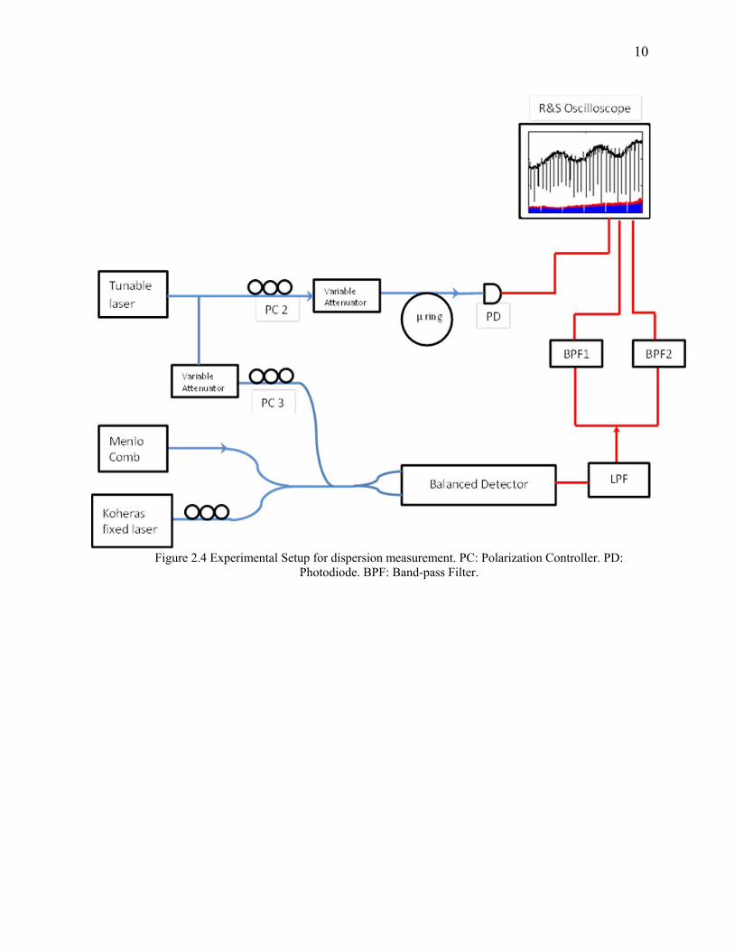
We use a similar experiment setup as described above. In our experimental, we used

New Focus tunable laser as the primary laser source. The laser has maximum sweeping

range from 1520nm to 1570nm and has advantage of small linewidth (≤200kHz). The

frequency comb is provided by MenloSystems optical frequency comb. The comb has

repetition rate of 250MHz. Finally, we use Koheras fixed wavelength laser as reference

to retrieve absolute frequency of the markers. Figure 2.4 shows the schematic diagram of

the setup. We coupled fixed wavelength laser with the optical frequency comb. A

polarization controller (PC) is used to adjust relative polarization of fixed wavelength

laser relative to the optical frequency comb. Changing the polarization will also change

the power coupled to the frequency comb. Tunable laser is set to the sweep mode and the

sweeping range is set to 1520nm to 1570nm. A 50:50 coupler is placed after the tunable

laser. 50% of the light will beat with the optical frequency comb to create frequency

markers, the other 50% is sent into the micro ring so that the transmission spectrum is

generated synchronously with the frequency markers. A balanced detector is used to

reduce the common noise in the beat signal. A low pass filter is used to filter out is placed

after the balanced detector to filter out the unwanted higher frequency in the beat signal.

Two narrow band band-pass filters are placed after the balanced detector and low pass

filter to generate frequency markers. The band-pass filters center at 30MHz and 75MHz

each. Therefore, for every m*250MHz, we would have 4 frequency markers at

m*250MHz±75MHz and m*250MHz±30MHz.

10

Figure 2.4 Experimental Setup for dispersion measurement. PC: Polarization Controller. PD: Photodiode. BPF: Band-pass Filter.

11

Since the tunable laser is sweeping continuously and we can’t read wavelength at

any instance, we are not able to retrieve the exact frequency of frequency markers.

Therefore, we use a fixed wavelength laser as a reference to find the absolute frequency

of the frequency markers. Four markers will be generated when the tunable laser

wavelength is close to the wavelength of the fixed wavelength laser. In order to distinct

these frequency markers from those generated from the beats between tunable laser and

the optical frequency comb, we would adjust the polarization controller and variable

attenuator until we see the reference markers that have greater amplitude compared to

other frequency markers.

2.3 Equipment Characteristic and Setting

In this section, we will discuss about the setting for the tunable laser and the

frequency response of the filters will be verified. We will also verify the output

wavelength and the uncertainty of the reference laser. Finally, the setting of the

oscilloscope will be reviewed.

If the experiment setup is correct, the resonances will be symmetric. The asymmetric

resonances usually result from the input laser power is too high or the laser sweep speed

is too fast. As described in [19], if the input laser power is too strong, the resonance will

be red shifted. Figure 2.4 shows the comparison between symmetric resonance and

asymmetric one. In figure 2.4(b), since the peak location of the asymmetric resonance

will not be at the center of the resonance, extra error will be introduced to the FSR, and

thus affects the dispersion. In order to keep the resonance symmetric, we would usually

adjust the variable attenuator so that the power before entering micro ring to around -

30dBm to -25dBm, which corresponds to 1μW to 3.16μW.

12

Figure 2.5 (a) A symmetric resonance captured by the oscilloscope. (b) Shows an asymmetric

resonance.

In order to ensure the resonance are symmetric, we have to make sure the rise time of

the photo-detector used to obtain the optical spectrum is shorter than the time it takes to

sweep over any resonance. We set the laser sweep speed to 11nm/s and would like to

know if the sweeping speed is too fast. First, we want to make sure that the Q factor is

not degraded by the photodiode rise time. That is, we can’t obtain the highest Q factor

because the photodiode rise time is long compared to laser sweep speed. By fitting the

resonance with Lorentzian curve, we are able to find the full width half maximum

(FWHM) of the resonance, and the Q factor of the resonance is calculated by:

∆(2.8)

We found that the Q factor of the resonance shown in figure 2.6 is around 106, which

match with the value obtained before. Now we would like to know how long it takes for

the laser to sweep over this wavelength range. This can be easily checked on the

oscilloscope and we found that the time is about 300μs as shown on figure 2.7. As

defined in the datasheet of the photo-diode we used for capturing transmission spectrum,

the rise time of the photo-detector can be calculated by:

0.35 ∗ 2π ∗ R ∗ (2.9)

13

is the diode capacitance as defined in the specification sheet and we used a 100kΩ

resistor for RLoad. The rise time of the photo-detector is found to be 4.84 μs. Therefore,

the resonance is symmetric and we conclude that it is reasonable to set laser sweep speed

to 11nm/s.

Figure 2.6 Curve fitting with Lorentzian distribution. The Q factor of the resonance is found to be around

106.

Figure 2.7 The resonance is captured in oscilloscope. It takes about 300μs to sweep over this resonance

when the laser sweep speed is 11nm/s.

1565.843 1565.844 1565.845 1565.846 1565.847

0

0.05

0.1

0.15

0.2

0.25

0.3

0.35

Wavelength (nm)

Am

plit

ude(

V)

DataFitted curve

4.7444 4.7445 4.7446 4.7447

0

0.05

0.1

0.15

0.2

0.25

0.3

0.35

Time(s)

am

plitu

de

(V)

14

Next we would like to check the frequency response of the band-pass filter and low-

pass filter. As mentioned above, we are using narrow-band band-pass filters to get

frequency markers. The pass band is of interest to us. We use Agilent vector network

analyzer (VNA) to test the frequency responses of both band-pass filters. Figure 2.7 is the

response of the 75MHz and 30MHz band-pass filters. The -3 dB pass band is tested to be

1.19MHz for 75MHz band-pass filter and 1.39MHz for 30MHz band-pass filter.

Figure 2.8 Frequency response of the band-pass filter used for frequency markers. (a) The response of

30MHz band-pass filter. (b) The response of 75MHz band-pass filter.

Next we would like to check the frequency response of the low-pass filter. The

frequency response of the low pass filter is important since we want to make sure that

higher beat frequency generated by mixing diode laser and Menlo comb won’t overlap..

Figure 2.9 shows the frequency response of the low pass filter. The -3dB pass band of the

low-pass filter is 118.15MHz.

15

Figure 2.9 Frequency response of the low pass filter.

We used a fixed wavelength laser to retrieve the absolute frequency of the frequency

markers and transmission spectrum of the micro-ring. Therefore, we would like to know

the output wavelength and the stability of the laser. We used wavelength meter to

measure the wavelength of the fixed laser around 5 minutes. The result is shown in figure

2.10. The average wavelength over the time interval is 1541.76206 nm and the

uncertainty is 0.000038nm.

0 100 200 300 400 500-60

-50

-40

-30

-20

-10

0

10

Am

plitu

de

(d

B)

Frequency (MHz)

16

Figure 2.10 The wavelength variation of the fixed laser around 5 minutes. It is found that the wavelength is

around 1541.76206±0.000038nm.

Finally, we would like to discuss about the setting for the oscilloscope. We used

Rhode & Schwarz RTO oscilloscope for the experiment. We want to make sure that there

is enough sample points for sampling both the transmission spectrum and the frequency

markers. The sampling frequency is fast enough as long as there are more than two

(which is the worst case scenario) sample points for each frequency marker. We

determined the required sampling rate through experiment and found that it will be

enough if the sampling rate is greater than 2.5M sample per second. It is observed that

there are around 10 points for one frequency marker, and the maximum of the frequency

marker can be captured. In order to get the frequency markers correctly, we have to set

those 2 channels to peak detect mode. The peak detect mode will record the maximum

and minimum value of the signal over the sampling time interval. The oscilloscope has

two load impedance with 50Ω and 1MΩ each. In order to increase to signal to noise ratio

(SNR) of both the transmission spectrum and frequency marker, we would prefer the

1MΩ resistor over the 50Ω resistor. For the transmission spectrum, we would put a

parallel resistor of 100 kΩ to reduce the load resistor and shorten the rise time of the

photo detector.

0 50 100 150 200 250 3001541.7619

1541.762

1541.7621

1541.7622

1541.7623

time (s)

wa

vele

ngth

(nm

)

17

2.4 Algorithm for Processing Frequency Marker Data

In this section, we would like to introduce the algorithm for retrieving the frequency

markers and resonance frequency from the transmission spectrum. Either missing a

frequency marker or mistaking a noise as a frequency marker will make the resonance

frequency erroneous.

First, in order to distinguish the marker from the noise background, we have to

define a threshold that we would recognize a marker is present if the amplitude is greater

than the threshold. However, the threshold can’t be set too high that we might miss some

frequency marker. Therefore, we use a moving average threshold that will be adjusted

dynamically according to the local frequency marker amplitude. The dynamic average is

useful because the power of the frequency comb and the tunable laser would increase

from 1530nm to 1570nm. Therefore, the amplitude of the frequency markers has 3 times

greater amplitude at 1570nm than 1530nm. The moving average threshold is used to

reduce the chance of finding error marker.

We would like to discuss how we find the peak of the frequency marker here. The

process is shown in Figure 2.11. We find the index where the amplitude is higher than the

threshold and define it as the start of the frequency marker, which is point A in the figure.

Then we define the index of the end of frequency marker B by finding the location where

the amplitude is lower than the threshold after point A. This is the range of a frequency

marker, and we simply find the local maximum between these 2 indexes to get the

frequency marker peak. However, we would like to jump over certain range after we find

a frequency marker peak to avoid recognizing the transient response of the band-pass

filter as a marker. If the sampling rate is around 2.5M sample/s, the jump range of 10~15

samples will be enough. Finally, we use this index as the starting point to find next

frequency marker peak, and the process repeat until we reach the end of data captured by

the oscilloscope.

(a) (b)

18

Figure 2.11 (a) A minimum threshold is set to distinguish frequency marker from noise background. Point

A is defined to be start of a frequency marker and B is end of frequency marker. (b) A small jump is introduced to avoid the transient response of the band-pass filter is captured as well.

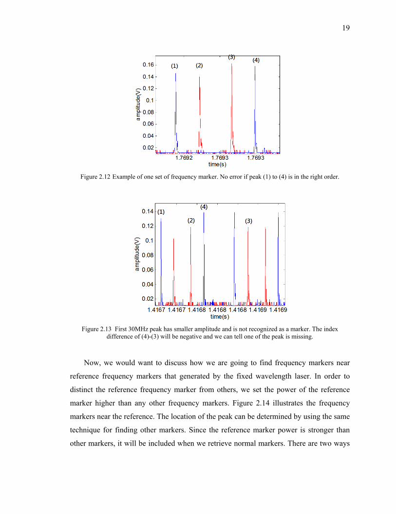
After the peak finding process is complete, we have to check if there are either

missing markers or noise peak being recognized as a marker. We define -75MHz, -

30MHz, 30MHz, and 75MHz frequency markers relative to a comb line of the frequency

comb as a set. Figure 2.12 shows a set of frequency markers. We can determine if there is

any acquisition error if we check the relative position between 30MHz peaks and 75MHz

peaks. Referring to figure 2.12, if we get one full set, the index difference of (peak2-

peak1), (peak3-peak1), (peak 4-peak 2), and (peak 4-peak 3) will be positive. We can

perform this check for every set of 4 frequency markers we acquired and the error can be

detected if any of the difference changes sign. If one of the peaks has smaller amplitude

and not recognized as a marker as shown on figure 2.13, the index difference (peak 4-

peak 3) will be negative, and we can tell one of the 30MHz peak is missing.

19

Figure 2.12 Example of one set of frequency marker. No error if peak (1) to (4) is in the right order.

Figure 2.13 First 30MHz peak has smaller amplitude and is not recognized as a marker. The index

difference of (4)-(3) will be negative and we can tell one of the peak is missing.

Now, we would want to discuss how we are going to find frequency markers near

reference frequency markers that generated by the fixed wavelength laser. In order to

distinct the reference frequency marker from others, we set the power of the reference

marker higher than any other frequency markers. Figure 2.14 illustrates the frequency

markers near the reference. The location of the peak can be determined by using the same

technique for finding other markers. Since the reference marker power is stronger than

other markers, it will be included when we retrieve normal markers. There are two ways

20

to rule out these markers: first is compare the amplitude of reference markers to normal

threshold. If it is several times higher, we can determine that this is a reference marker.

The other way we can simply check the index of the smaller amplitude frequency

markers we found and compare with the index of reference marker we already known.

Figure 2.14 (a) Frequency markers near the reference marker. The magenta circle represents the frequency markers retrieved. The light green circle is the reference markers. (b) Zoom in picture of the frequency marker where the marker almost overlaps with the reference. Since they don’t actually overlap, we can

retrieve this marker without error.

21

One problem that would occur with this setup is when the reference peaks overlap

with normal frequency markers. In that case, we will have a missing marker. To solve

this problem, we can calculate the index spacing between the reference markers we

already know. Although the laser sweeping speed is not constant during the scan, the

reference markers and local frequency markers are close enough that we can consider

they have same sweep speed. Therefore, we can use the index spacing between reference

markers to predict the location of the missing one. If there is a reference marker near that

location, we assume that those 2 markers overlap.

Occasionally, we observe noise beat note in our data. The beat note would have

similar amplitude to the frequency marker and make it hard to distinguish noise beat note

from the marker. With some trial and error, we determine that it is due to the locking

state of Menlo comb. This problem can be solved by relocking Menlo comb.

2.5 Algorithm for Processing Transmission Data

The algorithm for finding cavity resonances is similar to that for the frequency

marker. However, since there is more uncertainty in the transmission data, we have to

manually determine several parameters. First, there is high-frequency noise present in

the transmission data, so we utilize digital low-pass filter to smooth the spectrum. In

addition, sometimes we would observe change in transmission background power that is

caused by either tunable laser or variable attenuator. Therefore, we will filter out a small

part of low frequency components near DC of the transmission data to make the

background flatter. To find the location of the cavity resonance, we use similar technique

to finding the frequency markers. A threshold will be defined, but the threshold is

manually determined since every device has different coupling loss and we usually have

different power at the photo-detector. Occasionally, we will observe some of the

resonances have very small extinction. Therefore, we have to add some of the resonances

manually when it occurs.

A major difficulty that limits our ability to find dispersion accurately is the double

peaks at the resonance peak. We observe that there are double peaks at some resonance

22

peaks in a number of micro-resonators. The splitting of the resonance peak may result

from backward propagating wave induced by the scattering of light at coupling region or

surface roughness [20]. In such case, we will not be able to find the exact location of the

resonance peak. Figure 2.10 shows a resonance with double peak. We used 2 methods to

overcome this issue. One choice is the fit the resonance. By fitting the resonance with the

Lorentzian function, we may be able to find the peak of the resonance even if there is a

double peak present. The second choice is not to take the resonance into account.

However, this method sometimes would make the curve fitting unreliable. Therefore, the

first method is preferred over the second one.

Figure 2.10 Double peak resonance is sometimes found in the transmission spectrum. The location of peak

can’t be determined.

3.55 3.5505 3.551 3.5515 3.552 3.5525 3.5530.8

0.9

1

1.1

1.2

1.3

1.4

1.5

Time(s)

am

plit

ud

e(V

)

23

3. EXPERIMENTAL RESULT

In this chapter we will discuss the dispersion measurement result we obtained. The

majority of the device we measured has waveguide height of 550nm, 595nm, and around

800nm. In general, we would expect the dispersion to be normal dispersion for 550nm

device and anomalous dispersion for 800nm device. The device with 595nm waveguide-

height devices has dispersion falls in between. In addition, the uncertainty of the

dispersion measurement will be discussed. We were able to have accurate measurement

for some of the devices. Finally, we will briefly discuss the mode coupling phenomena. It

was observed that when two different modes cross each other, the local dispersion would

be modified.

3.1 Dispersion of Different Waveguide Dimension

We would like to show some dispersion measurement results in this section. The first

micro-ring sample has waveguide height of 430nm, and waveguide width of 2μm. The

ring radius is 200μm. Figure 3.1 shows the microscopic figure of the microring and

cross-section of the waveguide. The silicon nitride is deposited on top of silicon dioxide

substrate, and then the top of waveguide is covered with a silicon dioxide layer. Figure

3.2(a) shows the transmission spectrum of the device. One of the resonances was found to

be double peak. The zoom-in picture of the double peak is shown in figure 3.2(b). The

transmission spectrum in figure 3.2 is reconstructed with the retrieved frequency markers.

Since we didn’t use reference laser while doing this measurement, the frequency is

relative frequency instead of exact frequency.

24

Figure 3.1 (a) Microscope view of the micro-ring. (b) Cross-section illustration of the micro-ring.

Figure 3.2 Transmission spectrum of the device with 430nm 2μm dimension. (a) The transmission

spectrum of the device. The x axis is the relative frequency obtained by frequency marker. The real frequency is unknown since the reference laser wasn’t included. (b) Zoom in view of the peak mark as ‘x’

in (a). The peak has double peak feature, so we exclude that from our FSR fitting.

SiO2

Si3N4

25

It is obvious that only 1 mode with significant extinction ratio, so the FSR retrieval is

trivial. FSR evolution is shown in Figure 3.3. By fitting the curve of FSR evolution, we

obtained the dispersion of this device to be -1058.7 ps/nm/km. The negative value means

that the micro-resonator has normal dispersion. We can figure out if the micro-ring has

either normal or anomalous dispersion from the FSR evolution. If the FSR is decreasing

with higher frequency, we can interpret that as the refraction index is increasing as the

frequency increase, which is the definition of normal dispersion. In contrast, if the FSR is

proportional to the frequency, the micro-ring has anomalous dispersion.

Figure 3.3 FSR evolution and the fitting curve of the experimental data. Dispersion can be calculated from

the parameters of the curve fitted.

Next we would like to show the measurement result of a device with multiple modes.

When there is more than one mode, we have to group resonances to the same mode

family. The micro-ring we tested has waveguide height of 790nm, waveguide width of

2µm, and the ring radius is 100µm. The raw data we acquired is shown in figure 3.4. The

x-axis of the figure is time on the oscilloscope. The time it takes to capture all data is

around 4.55 second since we set the sweep speed to 11nm per second, and we set time

range to 4.7 second to ensure every resonances is included.

-6000 -5000 -4000 -3000 -2000 -1000 0119.6

119.8

120

120.2

120.4

120.6

Relative optical frequency (GHz)

FS

R (

GH

z)

NIST Gen1 Chip5 Ch.1

linear fitexperimental data

26

26

Figure 3.4 Transmission data captured by the oscilloscope. We have filtered the noise and the background by the digital filters. The two mode families are

assigned separately as shown in the figure. One mode is assigned to red “x”, while the other mode is assigned to black “x”.

0.5 1 1.5 2 2.5 3 3.5 4 4.5

0

0.05

0.1

0.15

0.2

0.25

0.3

0.35

0.4

0.45

0.5

Time(s)

am

plitu

de

(V)

27

The mode family is assigned manually when the 2 modes cross each other. For this

device, we observed that the Q factors of the two modes are different; thus, it is easy for

us to organize the resonances to different mode families. We didn’t observe any double

peak in this transmission spectrum; however, we found that there is significant change in

FSR evolution which is caused by the mode interaction phenomena. When the two

resonances are close, it is observed that different mode families would interact with each

other and change the local dispersion [3] [21] . Referring to figure 3.5(a) and (b), the last

data of the FSR corresponds to the first 2 resonances in transmission spectrum in figure

3.4 since the tunable laser is sweeping from low to high wavelength. We observe a

common FSR change in both mode 1 and 2. In order to obtain a better fit to the FSR

evolution, we would not take those FSR data into account for the curve fitting. In

addition, it is also observed that there is a significant FSR change at the first FSR data of

mode 1. To understand why there is a significant FSR jump, we again check the

resonance from transmission spectrum. The spectrum is shown in figure 3.6, and the

zoom-in picture of the resonance corresponds to the first FSR data of mode 1 is shown in

figure 3.6(b). It is found that there is a small extinction ratio resonance which is belonged

to TM polarization. Therefore, we conclude that the significant FSR jump is result from

the mode interaction between TE and TM polarization mode.

Figure 3.5 FSR evolution of the two modes from TE polarization. (a) FSR evolution of the mode family 1.

We observe mode interaction in the first and last data. (b) FSR evolution of the mode family 2.

28

Figure 3.7 FSR evolution of the mode family 1 and 2 with mode interaction point excluded. Figure 3.5(a)

is the FSR evolution of mode 1. (b) FSR evolution of mode 2

Finally, in figure 3.7, the FSR evolution and the curve fitted is shown. We found the

dispersion of this micro-ring to be 337.55ps/km/nm for mode family 1 and

52.02ps/km/nm for mode 2.

Figure 3.6 (a) Transmission spectrum of the micro-ring. The x-axis is the absolute frequency. (b) The first resonance of the transmission spectrum as indicated in (a). We found that there’s a smaller extinction ratio resonance which corresponds to

mode from TM polarization.

29

Other measurement results are shown in table 3.1 and 3.2. We observe some

agreement for the device with same dimension. However, we do have several

measurements having different values for the same waveguide width and height. From

table 3.1, we can see that the error tend to be higher if the waveguide width is wider. This

is anticipated since with wider waveguide width, we would observe more modes in the

transmission spectrum. This leads to more mode coupling and introduce more abrupt FSR

change.

Table 3.1 Dispersion measurement of different devices. We see some agreement for the devices with same dimension. Some of the measurement has higher error since the FSR evolution is not well fitted.

Device Waveguide

Width

(μm)

Waveguid

e Height

(nm)

TE Mode 1

Dispersion(ps/

nm/km)

TE Mode 2

Dispersion(ps/n

m/km)

TE Mode 3

Dispersion(p

s/nm/km)

Purdue

033014

595nm

A1 Ch13 2 595 -61.99±15.77 16.68±24.31

A2 Ch5 2 595 -108.83±36.47 30.02±42.66

A2 Ch6 2 595 -79.68±44.02 -36.96±53.79

A2 Ch7 2 595 -90.86±17.35 -13.29±25.36

A2 Ch8 3 595 70.21±18.26 150.59±41.55

A2 Ch9 3 595 4.09±56.07 169.69±100.59

Purdue

033014

790nm

A1 Ch12 2 790 39.27±7. 70 340.13±42.29

A1 Ch13 2 790 47.51±7. 74 336.18±14.04

A1 Ch19 3 790 4.85±41.27 144.42±37.22 452.28±107.

23

A1 Ch19

drop port

3 790 -2.47±39.21 153.62±26.52

A2 Ch9 3 790 178.36±50.10 397.84±63.8

2

A2 Ch10 3 790 161.62±38.19 411.8±79.81

A2 Ch11 3 790 220.72±62.13 380.29±75.2

30

2

Table 3.2 Dispersion measurement of different devices continued. Device Waveguide

Width (μm)

Waveguide

Height

(nm)

Mode 1

Dispersion(ps/

nm/km)

Mode 2

Dispersion(ps

/nm/km)

Purdue

072313

550nm

B4 Ch10 2 550 -789.26

B4 Ch11 2 550 -538.13 -719.37

B4 Ch11

drop port

2 550 -552.13 -729.36

B4 Ch11

TM mode

2 550 -57.97 -204.65

Purdue

072313

800nm

B1 Ch4 2 800 100.31

B1 Ch4(2) 2 800 81.77±86.51

B4 Ch11 2 800 81.86±17.68 259.47±30.11

NIST Gen5 Ch1 2 430 -1058.7±25.36

31

In order to verify if our measurements are reasonable, we would like to compare the

measured values to simulated ones. We ran the simulation with free software MIT

Photonics Band (MPB). The total cavity dispersion includes the material dispersion and

the geometry dispersion while the material dispersion is calculated based on Sellmeier’s

Equation. In addition, we assumed all waveguides has an etching angle of 5 degree. The

comparison between simulation and measured dispersion is shown in table 3.3. From

table 3.3, we do see some agreement between the measured and simulated dispersion.

However, we found a great mismatch at waveguide height of 550nm and width of 2 μm.

The possible reason for this mismatch is that the dispersion we measured might not be the

fundamental mode.

Table 3.3Comparison between simulated dispersion and measured one Waveguide Width

(μm)

Waveguide Height

(nm)

Simulated

Dispersion(ps/nm/km)

Measured

Dispersion(ps/nm/km)

2 550 -170 -538.13

2 600 -78 -108.83±36.47

2 800 59.9 47.51±7. 74

3 800 21.5 4.85±41.27

32

Figure 3.8 FSR error analysis for mode 1 (a)FSR deviations for the resonances from 1520nm to 1570nm

from 70 measurements. The standard deviation of FSR is 4.7MHz. (b) Simulated dispersion by applying an error to each of the FSR. The error of the FSR is assumed to be the standard deviation.

0 5 10 15 20 25227.5

227.52

227.54

227.56

227.58

227.6

227.62

227.64

FS

R (

GH

z)

FSR number

20 40 60 80 1000

0.02

0.04

0.06

0.08

0.1

0.12

0.14

0.16

Dispersion (ps/nm/km)

Pro

bab

ility

SimulatedGauss fitted

(a)

(b)

33

Figure 3.9 FSR error analysis for mode 1 (a)FSR deviations for the resonances from 70 measurements. The standard deviation of FSR is 6.24MHz. (b) Simulated dispersion by applying an error to each of the FSR.

The error of the FSR is assumed to be the standard deviation.

0 5 10 15 20 25219.4

219.5

219.6

219.7

219.8

219.9

220

FS

R (

GH

z)

FSR number

300 320 340 360 3800

0.02

0.04

0.06

0.08

0.1

0.12

Dispersion (ps/nm/km)

Pro

bab

ility

SimulatedGauss fitted

(a)

(b)

34

3.2 Error Analysis of the Dispersion Measurement

In this section we would like to discuss the method we used to estimate the

uncertainty of the dispersion measurement. In order to retrieve the uncertainty in our

measurement, we performed measurement experiment on one micro-ring multiple times.

The micro-ring we chose is channel 13 of Purdue 033014 790nm. The dimension of the

chip is 790nm height, 2μm width, and the ring radius is 100µm. We maintained the same

setup and performed the measurement 70 times. As discussed in section 3.1, we don’t

take the FSR that has mode interaction into account. The uncertainty of the FSRs for each

mode family is shown in figure 38 and 3.9. In figure 3.8(a), the x-axis is the number of

FSR we assigned to avoid ambiguity. We then found the standard deviation of FSRs

to be 4.7MHz from the measurements. To estimate the uncertainty of dispersion, we

assume each FSR has a normal distribution and simulate the curve fitting. We then

simulate the FSR evolution and fit the curve for each of them and calculate the dispersion.

The result is shown in figure 3.7(b). Finally, we choose the standard deviation of the

dispersion value obtained previously as the uncertainty. For mode family 1 of this micro-

ring, we find dispersion D = 52.02±2.52ps/nm/km. We perform similar process for mode

family 2 and the result is shown in figure 3.8. The dispersion value and uncertainty is

337.55±4.11ps/nm/km.

Next we perform error analysis for Purdue B4 channel 11. The dimension of the chip

is 800nm height, 2μm width, and the ring radius is 100µm. We did the measurement 30

times while setting the laser to sweep from 1540nm to 1560nm. The shorter sweeping

range is chosen because the time it takes to save full range data is long. The deviation of

each of the FSR is shown in figure 3.6. Again, we calculate the standard deviation of

FSRs and simulate the FSR evolution. The error of the dispersion is determined by

simulating the dispersion with the uncertainty of FSR we obtained. Figure 3.11 shows the

simulation result with size of 50,000. Finally, we concluded the dispersion of this device

is 81.82±17.68ps/nm/km.

35

Figure 3.10 FSR deviations for the resonances from 1540nm to 1560nm. The maximum deviation of the

FSR is around 200MHz.

Figure 3.11 Dispersion simulations with size of 50,000. Again the error of FSR is assumed to be the

standard deviation of FSR variation.

0 2 4 6 8 10220.95

221

221.05

221.1

221.15

221.2

221.25

221.3

FS

R (

GH

z)

FSR number

-100 -50 0 50 100 150 200 250 3000

0.02

0.04

0.06

0.08

0.1

0.12

Dispersion(ps/nm/km)

pro

bab

ility

36

There are several factors that might contribute to the error. The first one is the

nonlinearity of the laser sweep speed. Although we acquire the frequency markers and

transmission spectrum synchronously, we still can’t resolve the frequency between any 2

frequency markers. We used interpolation to find the relative frequency, but there is

uncertainty if the laser sweep speed change abruptly. Another factor is the Q factor of the

resonances. If the Q factor is higher, there is less error for the peak of the resonance, and

we would expect a more accurate result. The noise in the transmission spectrum will

introduce error to the dispersion as well, but it can usually be reduced with implementing

digital low pass filter.

To verify how much error can be introduced by the laser sweep speed nonlinearity,

we again measured another device – Purdue 072313 800nm B1 Ch4. Due to the fact that

we choose arbitrary starting point of frequency marker and the data we obtained would

shift a little bit in time scale in every measurement, there’s an offset between different

measurements. We chose a specific resonance as reference to align other resonances and

find the offset. However, we found that the frequency variation of other resonances being

around 400MHz to 500MHz. The variation is very large thus makes the measurement

unreliable. Referring to table 2, the dispersion and error for this device is

81.77±86.51/nm/km. Although we can’t find out why the error is large for this device, we

do observe some devices would have greater uncertainty even they have same dimension.

For some of the device, we didn’t perform multiple measurements. Therefore, we

chose the difference between the fitted FSR and the experimental FSR data to be the

variation of the FSR. Then we find the standard deviation of these variations and

assumed it to be the error of FSRs. The error is usually found to be smaller. It is less

reliable than the error we obtained from multiple measurements; however, we do see that

when the FSR variation between fitted curve and actual data are larger, the errors we get

from multiple measurements are larger as well. Therefore, it does provide an estimate of

error we are going to expect.

37

3.3 Mode Interaction

If there is more than one mode family in the spectrum and they have different FSR,

the modes would eventually cross in the transmission spectrum. From the experiment, we

found that the FSR of the local resonances would be modified by the interaction between

two modes. Figure 3.8 shows the result of mode interaction. We observe that the FSR of

one mode suddenly increased while the FSR of the other mode decreased. The amount of

FSR increased is similar to the amount decreased at the other mode. In addition, we

observed that when two modes are close to each other, their Q factor will be modified as

well. The mode with higher Q will have Q factor decreased while the mode with lower Q

factor will exhibit higher Q factor. The mode interaction phenomenon is related to the

initiation of micro-resonator frequency comb generation in normal group velocity

dispersion [21].

Figure 3.8 When there’s mode interaction, a sudden FSR change is observed.

38

4. CONCLUSION AND FUTURE WORK

We have accomplished measuring the dispersion with the aid of frequency comb. We

were able to implement signal processing algorithm to reduce the noise in the raw data

and the dispersion of several different micro rings is measured. The accuracy of

measurements is a very important factor and we are able to obtain an accurate

measurement. Experimental result shows that we can measure the dispersion within 10%

error for certain devices. In addition, we have found a good match between measured and

simulated dispersion. However, there are several problems weren’t solved.

First, we still observe large variation in FSR data for some of the devices. The large

variation in FSR may result from the defect in micro rings. Secondly, we don’t have a

good match between simulation and experimental data for micro ring with 550nm

waveguide height micro-ring. As mentioned above, the mismatch might come from that

the simulated and measured dispersion was for different modes. Finally, although we can

measure the dispersion with decent accuracy, it is possible to further increase the

precision. Due to the fact that we only use 2 band-pass filters at 30MHz and 75MHz, we

can’t resolve the precision between any 2 markers. The interpolation method is used to

increase accuracy but if laser sweep speed changes abruptly during 2 markers the

accuracy is reduced. Therefore, it would be viable to add one more band-pass filter and

reduce the frequency spacing between frequency markers. This will in turn increase the

accuracy of the measurements.

8

LIST OF REFERENCES

8

LIST OF REFERENCES

[1] T. Udem, R. Holzwarth, and T. W. Hansch, "Optical frequency metrology," Nature,

vol. 416, pp. 233-237, 2002.

[2] J. Reichert, M. Niering, R. Holzwarth, M. Weitz, T. Udem, and T. W. Hänsch,,

"Phase Coherent Vacuum-Ultraviolet to Radio Frequency Comparison with a Mode-

Locked Laser," Physical Review Letters, vol. 84, pp. 3232-3235, 2000.

[3] Del’Haye, P. et al., "Frequency comb assisted diode laser spectroscopy for

measurement of microcavity dispersion," Nat Photon, vol. 3, pp. 529-533, 2009.

[4] J. A. Stone and P. Egan, "An Optical Frequency Comb Tied to GPS for Laser

Frequency/Wavelength Calibration," Journal of Research of the National Institute of

Standards and Technology, vol. 115, pp. 413-431, 2010.

[5] C.-B. Huang, Z. Jiang, D. E. Leaird, and A. M. Weiner, " High-rate femtosecond

pulse generation via line-by-line processing of phase-modulated CW laser frequency

comb," Electronics Letters, vol. 42, pp. 1114-1115, 2006.

[6] A. M. Weiner, Ultrafast Optics, John Wiley & Sons, Inc, 2008.

[7] Del’Haye, P. et al., "Optical frequency comb generation from a monolithic

microresonator," Nature, vol. 450, pp. 1214-1217, 2007.

[8] T. J. Kippenberg, R. Holzwarth and S. A. Diddams, "Microresonator-based optical

8

frequency combs," Science, vol. 332, pp. 555-559, 2011.

[9] M. A. Foster, J. S. Levy, O. Kuzucu, K. Saha, M. Lipson, and A. L. Gaeta, "Silicon-

based monolithic optical frequency comb source," Optics Express, vol. 19, pp.

14233-14239, 2011.

[10] T. Herr, K. Hartinger, J. Riemensberger, C. Y. Wang, E. Gavartin, R. Holzwarth, M.

L. Gorodetsky & T. J. Kippenberg, "Universal formation dynamics and noise of

Kerr-frequency combs in microresonators," Nature Photonics, vol. 6, no. 7, pp. 480-

487, 2012.

[11] Ivan S. Grudinin et al., "Frequency comb from a microresonator with engineered

spectrum," Optics Express, vol. 20, no. 6, pp. 6604-6609, 2012.

[12] P.-H. Wang, F. Ferdous, H. Miao, J. Wang, D. E. Leaird, K. Srinivasan, et al,

"Observation of correlation between route to formation, coherence, noise, and

communication performance of Kerr combs,," Optics Express, vol. 20, pp. 29284-

29295, 2012.

[13] Victor Torres-Company et al., "Comparative analysis of spectral coherence in

microresonator frequency comb," Optics Express, vol. 22, no. 4, pp. 4678-4691,

2014.

[14] P. Del’Haye, T. Herr, E. Gavartin, M. L. Gorodetsky, R. Holzwarth, and T. J.

Kippenberg, "Octave Spanning Tunable Frequency Comb from a Microresonator,"

Phys. Rev. Lett., vol. 107, no. 6, p. 063901, 2011.

[15] Yoshitomo Okawachi, Kasturi Saha, Jacob S. Levy et al., "Octave-spanning

8

frequency comb generation in a silicon nitride chip," Optics Letters, vol. 36, no. 17,

pp. 3398-3400, 2011.

[16] T. Herr, V. Brasch, J. D. Jost et al., "Temporal solitons in optical microresonators,"

Nature Photonics, vol. 8, pp. 145-152, 2014.

[17] K. Saha, Y. Okawachi, B. Shim, J. Levy, R. Salem, A. Johnson, M. Foster, M.

Lamont, M. Lipson, and A. Gaeta,, "Modelocking and femtosecond pulse generation

in chip-based frequency combs," Opt. Express, vol. 21, no. 1, pp. 1335-1343, 2013.

[18] A. B. Matsko, A. A. Savchenkov, and L. Maleki, "Normal group-velocity dispersion

Kerr frequency comb," Optics Letters, vol. 37, no. 1, pp. 43-45, 2012.

[19] L. Luo, G. Wiederhecker, K. Preston, and M. Lipson, "Power insensitive silicon

microring resonators," Opt. Lett., vol. 37, no. 4, pp. 590-592, 2012.

[20] Pei-Hsun Wang et al., "Drop-port study of microresonator frequency comb: power

transfer, spectra and time-domain characterization," Optics Express, vol. 21, no. 19,

pp. 22441-22452, 2013.

[21] Y. Liu, Y. Xuan, X. Xue, P. Wang, S. Chen, A. Metcalf, J. Wang, D. Leaird, M. Qi,

and A. Weiner,, "Investigation of mode coupling in normal-dispersion silicon nitride

microresonators for Kerr frequency comb generation," Optica, vol. 1, no. 3, pp. 137-

144, 2014.

[22] Jiang Li et al., "Sideband spectroscopy and dispersion measurement in

microcavities.," Optics Express, vol. 20, no. 24, pp. 26337-26344, 2012.

[23] Saha, Kasturi et al., "Modelocking and femtosecond pulse generation in chip-based

8

frequency comb," Optics Express, vol. 21, no. 1, pp. 1335-1343, 2013.

[24] Cyril Godey, Irina V. Balakireva, Aurélien Coillet, and Yanne K. Chembo,

"Stability analysis of the spatiotemporal Lugiato-Lefever model for Kerr optical

frequency combs in the anomalous and normal dispersion regimes," Phys. Rev., vol.

A 89, p. 063814, 2014.

[25] Lin Zhang et al., "Generation of two-cycle pulses and octave-spanning frequency

combs in a dispersion-flattened micro-resonator," Optics Letters, vol. 38, no. 23, pp.

5122-5125, 2013.

10

APPENDIX

15

APPENDIX