dissecting interfaces of antibody -antigen complexes: from
TRANSCRIPT

HAL Id: hal-01191462https://hal.inria.fr/hal-01191462
Submitted on 1 Sep 2015
HAL is a multi-disciplinary open accessarchive for the deposit and dissemination of sci-entific research documents, whether they are pub-lished or not. The documents may come fromteaching and research institutions in France orabroad, or from public or private research centers.
L’archive ouverte pluridisciplinaire HAL, estdestinée au dépôt et à la diffusion de documentsscientifiques de niveau recherche, publiés ou non,émanant des établissements d’enseignement et derecherche français ou étrangers, des laboratoirespublics ou privés.
Dissecting Interfaces of Antibody -Antigen Complexes:from Ligand Specific Features to Binding Affinity
PredictionsSimon Marillet, Marie-Paule Lefranc, Pierre Boudinot, Frédéric Cazals
To cite this version:Simon Marillet, Marie-Paule Lefranc, Pierre Boudinot, Frédéric Cazals. Dissecting Interfaces of Anti-body -Antigen Complexes: from Ligand Specific Features to Binding Affinity Predictions. [ResearchReport] RR-8770, Inria Sophia Antipolis. 2015, pp.61. �hal-01191462�

ISS
N02
49-6
399
ISR
NIN
RIA
/RR
--87
70--
FR+E
NG
RESEARCHREPORTN° 8770September 2015
Project-Team Algorithms-Biology-Structure
Dissecting Interfaces ofAntibody - AntigenComplexes:from Ligand SpecificFeatures to BindingAffinity PredictionsSimon Marillet and Marie-Paule Lefranc and Pierre Boudinot andFrédéric Cazals


RESEARCH CENTRESOPHIA ANTIPOLIS – MÉDITERRANÉE
2004 route des Lucioles - BP 9306902 Sophia Antipolis Cedex
Dissecting Interfaces of Antibody - AntigenComplexes:
from Ligand Specific Features to BindingAffinity Predictions
Simon Marillet∗ and Marie-Paule Lefranc† and PierreBoudinot‡ and Frédéric Cazals §
Project-Team Algorithms-Biology-Structure
Research Report n° 8770 — September 2015 — 58 pages
Abstract: Adaptive immunity is based on antigen-specific lymphocyte responses, with inparticular B cells secreting seric immunoglobulins (IG) involved in the opsonization of bacteriaand the neutralization of viruses. At the heart of these mechanisms is the formation of IG -Ag complexes, which challenge our understanding in terms of binding affinity and interactionspecificity.In this work, we dissect the interfaces of IG - Ag complexes with high resolution crystal structures,making a stride towards a better understanding of binding affinity and interaction specificity. First,we present global interface statistics clearly distinguishing ligand types (proteins, peptides, chem-ical compounds), and stressing the role of side chains. Second, we analyze the relative positions ofCDR with and without antigen, exhibiting a remarkably conserved pattern involving seven seamsbetween CDR. We also show that this generic pattern exhibits specific properties as a function ofthe ligand type. Finally, we present binding affinity predictions of unprecedented accuracy, with amedian absolute error of 1.02 kcal/mol.We anticipate that our findings will be of broad interest, not only in studying immune responsesat the structural level, but also in bio-engineering and IG design, with IG used extensively indiagnostics and as well as therapeutic agents.
Key-words: Antibody - antigen complex; interface ; affinity; relative CDR locations
∗ Inria and INRA (Unité de Virologie et Immunologie Moléculaires), France† IMGT, IGH, CNRS, France‡ INRA, Unité de Virologie et Immunologie Moléculaires, Jouy-en-Josas, France§ Inria, France

Analyse des Interfaces de complexes Anticorps - Antigène:des caractéristiques propres au type de ligand à la
prédiction d’affinité de liaisonRésumé : L’immunité adaptative est basée sur une réponse lymphocytaire spécifique del’antigène, les lymphocytes B sécrétant en particulier des immunoglobulines (IG) sériques im-pliquées dans l’opsonisation des bactéries et la neutralisation des virus. Au cœur de ces mé-canismes se situe la formation de complexes IG - Ag, défiant notre compréhension quant à laprédiction de l’affinité de liaison et de la spécificité des interactions.
Dans ce travail, nous disséquons les interfaces de complexes IG - Ag à partir de structurescristallographiques à haute résolution, faisant ainsi un pas en direction d’une meilleure com-préhension de l’affinité de liaison et de la spécificité des interactions. Premièrement, nous présen-tons des statistiques sur les interfaces dans leur globalité permettant de distinguer clairementles types de ligands et de souligner l’importance des chaines latérales. Deuxièmement, nousanalysons les positions relatives des CDR en contact ou non avec un antigène, exhibant ainsiun motif remarquablement conservé impliquant sept coutures entre les six CDR. Nous montronségalement que ce motif générique possède des propriétés spécifiques au type de ligand. En-fin, nous présentons des prédictions d’affinité d’une précision inégalée, avec une erreur absoluemédiane de 1.02 kcal/mol.
Ces résultats sont d’intérêt général, non seulement pour l’étude des réponses immunitairesau niveau structural, mais également pour l’ingénierie biologique et le design d’IG, celles-ci étantlargement utilisées pour les diagnostics et en tant qu’agents thérapeutiques.
Mots-clés : Complexe anticorps - antigène ; interface ; affinité; positions relatives des CDR

Dissecting Interfaces of Antibody - Antigen Complexes 3
1 Introduction
1.1 Immunoglobulins and the immune responseAdaptive immunity is based on antigen (Ag)-specific lymphocyte responses. Upon specific recog-nition of an antigenic epitope by a given receptor unique to a lymphocyte, this cell gets activatedand proliferates, leading to a clonal expansion. B lymphocytes thus recognizes the native antigenthrough immunoglobulins (IG) or antibodies on their membranes. Following differentiation oflymphocytes into plasmocytes, IG are then secreted and bind the antigen as a soluble receptor.Seric IG can opsonize bacteria and facilitate their uptake by phagocytes, or neutralize virusesthus preventing recognition by their receptor or fusion with the target cell. During the secondaryimmune response, affinity maturation is responsible for the secretion of IG of higher affinity, again of up to three orders of magnitude being common.
Immunoglobulins fundamentally consist of two identical heavy (H) chains and two identicallight (L) chains, each H chain being bound to an L chain by a disulfide bond and by noncovalentinteractions between the variable domains VH and VL and the constant domains CH1 andCL. The antigen-binding site is located at the top of the paired VH and VL, and generallyoverlaps the two V domains. It mainly consists of three flexible loops on each V domain, calledcomplementarity determining regions (CDR1-3) [72, 9].
Matching the universe of antigenic motifs specifically requires a very large diversity of recog-nition modes by immunoglobulins. This is achieved by a huge diversity of the loops constitutingthe antigen binding sites at the top of the VH and VL domains. The aforementioned CDR1 and2 are encoded by the V gene and their diversity depends on genes and alleles, whereas the CDR3loop corresponds to the site of the V(D)J rearrangements, which generate the highest sequencediversity [68], [55, Chapter 6].
1.2 IG - Ag complexes under the structural lensFrom the structural standpoint, the functional relevance of an IG is described by its bindingaffinity for the targeted antigen and the specificity of such interactions. The specificity is criticalto ensure that the response targets the antigen, and not, for example, a motif present on a selfprotein - and it is also the basis of immune memory and vaccination. The affinity sets the strengthof the interaction and the time the antigen and the antibody are linked to each other. For themembrane bound IG, it determines if enough aggregation of surface IG and IG co-receptorsoccurs, so that a sufficient signal can be sent to the cell to induce activation and proliferation;for secreted IG, it sets the efficiency of IG-mediated pathogen opsonisation and/or neutralization,or IG effector properties (antibody-dependent cell-cytotoxicity (ADCC), complement-dependentcytotoxicity (CDC)), after binding to the target infected or tumoral cells [42]. In mouse andhuman, secondary immune responses are often accompanied by affinity maturation, a processduring which B cells expressing IG with enhanced affinity are being selected. Such IG withhigher affinity result from the selection of random mutations of their V(D)J genes producedby the enzyme activation-induced cytidine deaminase (AICDA, AID), which may modify thestructure of the antigen binding site, hence the affinity of the interaction with the Ag.
The binding affinity is a thermodynamic parameter describing an equilibrium between threespecies, namely the partners and the complex they form. It is generally measured by a dis-sociation constant Kd of this equilibrium, or equivalently by the associated dissociation freeenergy. Thus, by nature, the affinity has enthalpic and entropic components. The enthalpiccomponent describes the interaction energy. Generically, given two partners forming a complex,various parameters have been proposed to model the complex. Most of these parameters tar-get the interface, and describe its size and morphology, shape (number of patches), biochemical
RR n° 8770

4 Marillet and Cazals
properties (salt bridges, solvation, H bonds), or packing properties and have been studied usingcrystal structures of complexes, see [33, 46, 8, 48] and the references therein. More recently, ithas also been shown that non-interacting atoms play an important role, intuitively related tosolvent interactions [35]. For the particular case of IG - Ag complexes, it has been observedthat interfaces tend to have a smaller size, have curvature dependent on the ligand size [47].The entropic component accounts for the dynamics of the partners. In particular, it has beenshown that preconfiguration/prerigidification of the binding site may yield a decreased entropicloss, hence a enhanced binding affinity [49, 59, 15, 60]. The specific role played in Ag bindingby CDR also prompted the analysis of CDR specific statistics. Using a handful of structures,canonical structures i.e. commonly occurring backbone CDR conformations were first reported[17] and subsequently updated [18, 2]. Moving from individual CDR to all CDR, correlationsbetween canonical structures were further studied [70], highlighting the fact that selected com-binations are multi-specific, while others are specific of an antigen type. The VH CDR3 is themost variable and was therefore the focus of several studies [62, 53, 64] which defined and up-dated sequence-based rules to predict its conformations. More recently, these studies have beenrefined, based on a larger number of structures (of the order of hundreds instead of tens). ForVL CDR3, new canonical structures were proposed [38], and for VH CDR3, previous rules wereupdated and complemented [36, 37]. The work of Chothia et al [17] was also refined using 300nonredundant IG structures and a pre-processing based on CDR length [54]. Distinguishinglambda versus kappa chains, it has been shown that canonical conformations from the formerare more diverse than those from the latter in the human and the mouse [13]. However, theuse of canonical conformations was questioned [16], since general prediction methods for loopsmatched (or even outperformed) the prediction performances of methods exploiting specific rulesassociated with canonical structures of CDR. Finally, two related works [3, 58] studied the dif-ferential CDR lengths and SDRU (proportion of structures contacting the antigen at a givensite) between ligand types. However, these analysis do not extend to predictions of the antigentype. More generally, the reader may consult [27] for a review of structural and genetic aspectsof natural and artificial antibody repertoires.
While the previous analyses certainly shed light on antigen recognition modes, they fallshort from providing complete information on binding affinity. Predicting binding affinities fromstructural data is a notoriously challenging problem, for protein complexes in general [34, 50],and for IG - Ag complexes in particular [45]. This actually owes to the intrinsic nature ofKd, namely a macroscopic property describing the chemical equilibrium associated with the twopartners (IG and Ag) and the complex (IG - Ag, denoted IG/Ag in the IMGT nomenclature[25]). That is, the magnitude of Kd has an enthalpic component, qualifying the strength of theinteraction, but also an entropic component qualifying the loss of dynamical properties uponcomplex formation – intuitively the formation of the IG - Ag complex restricts the degreesof freedom of both partners. These two competing interests illustrate the enthalpy - entropycompensation phenomenon [52, 24], which stipulates that a favorable enthalpic change uponassociation is accompanied by an entropic penalty. In [56] and [69] the authors have shown thata preconfiguration process of the variable domains can be induced by the constant domain 1(CH1) of the heavy chain, suggesting that the isotype switching commonly occurring during Bcell differentiation may affect the affinity through changes in the dynamic properties of the IG.Parallel to binding affinity, the notion of functional affinity or avidity which takes into account the(possibly negative) cooperativity between IG is highly relevant in-vivo. In that context, constantregions have been shown to influence the avidity [22, 23, 51, 57]. Likewise, am intact ball-and-socket joint between VH and CH1 domains has been shown to condition antibody neutralizingactivity [39].
Inria

Dissecting Interfaces of Antibody - Antigen Complexes 5
Contributions. This work sheds new light on IG - Ag interactions. We use the annotatedIMGT/3Dstructure-DB [25], focusing on canonical complexes, each such complex involving ex-actly one variable domain from the heavy chain (VH), one variable domain from the light chain(VL) and one antigen (Ag). Of particular interest is the ligand type (reduced to protein, pep-tide and chemical in this paper, see Section 2.3). Upon extracting canonical complexes from theIMGT/3Dstructure-DB, our analysis relies on hierarchical Voronoi interface models, and involvesthree main steps. IG atoms are first marked as belonging to CDR or framework regions (FR),using the IMGT unique numbering [43]. (Practically, we use the following notations: CDR1-IMGT of VH is written VH CDR1 and FR3-IMGT of VL is written VL FR3. Other CDR andFR follow the same scheme.) Subsequently, the interface between the IG chains and the Ag isdetermined using a Voronoi based model, and hierarchically decomposed into contributions fromCDR, FR and other atoms.
Using these tools, we present novel analysis for IG - Ag complexes, in three directions. First,we report global interface statistics, in particular as a function of the ligand type, stressing the roleof side chains and going beyond previous work solely based on backbone canonical conformations.In particular, these statistics discriminate between different ligand types, a key observation tounderstand binding specificity. Second, we present novel analysis of the relative contributions ofCDR to binding, highlighting the relative positions of CDR. We notably mitigate the classicalview of prominent contribution of CDR3 to the interface, showing that in terms of buried surfacearea, CDR3 on the one hand, and CDR1 + CDR2 on the other hand, must be considered on anequal footing. We also show that there exist a conserved pattern of contacts between CDR, withspecific properties depending on the antigen type. Finally, we present binding affinity predictionsof unprecedented accuracy.
2 Material and Methods
2.1 Voronoi Interface Models
Given a macro-molecular complex, an interface model is a structural model of the atoms account-ing for the interactions. Various interface models have been developed, based in particular ondistance thresholds and loss of solvent accessibility [4]. In the sequel, we use the Voronoi basedinterface model, which is a parameter free construction improving on previous models in severalaspects. Since we shall be using features of this model, we present it briefly. (See also Fig. 1 foran illustration on an IG - Ag complex.)
Solvent accessible models. The solvent accessible model (SAM) of a set of atoms is a modelwhere each atom is represented by a ball whose radius is the van der Waals radius expandedby the radius rw = 1.4Å of a water probe accounting for a continuous solvation layer [28, 4].A convenient construction to study SAM is the Voronoi (power) diagram defined by the atoms[28]. In particular, the Voronoi diagram induces a partition of the molecular volume, obtained bycomputing for each atom its Voronoi restriction, namely the intersection between its atomic balland its Voronoi region. The volume of a restriction can be used to define packing properties: theraw packing property of one atom is plainly the volume of its restriction; the normalized packingproperty is the volume of the restriction normalized by the volume of the corresponding ball.
Buried surface area. The exposed surface of a SAM consists of the boundary of the union ofballs defining the SAM. (Prosaically, the visible surface of the molecule.) This surface consists ofspherical polygons, delimited by circle arcs (every such arc is located on the intersection circle of
RR n° 8770
6 Marillet and Cazals
two atoms), themselves delimited by points (each such point is found at the intersection of threespheres). When two molecules assemble to form a complex, the buried surface area (BSA) is theportion of the exposed surface of the partners which gets buried [46]. BSA has been shown toexhibit remarkable correlations with various biophysical quantities [32], and notably dissociationfree energies for complexes involving moderate flexibility [48].
Voronoi interface. Consider the SAM of a complex whose partners are denoted A and B, andalso involving water molecules tagged W. Two atoms are in contact provided that their Voronoirestrictions are neighbors. Pairs of type (A,B) define the AB interface, namely direct contactsbetween the partners. Focusing on W molecules sandwiched between the partners, pairs (A,W)and (B,W) correspond to water mediated interactions. It can be shown that all atoms fromthe partners identified this way form a superset of atoms loosing solvent accessibility [12]. Thebinding patch of a partner consists of its interface atoms. The atoms of the binding patch canbe assigned an integer called its shelling order, which is a measure of the distance of this atomto the boundary of the patch it belongs to [8]. This information generalizes the core-rim model[46], and has been shown to provide STAR correlations with solvent dynamics, conservation ofamino acids [8], and dissociation free energies [48].
The Voronoi facets associated to pairs of type (A,B) define the bicolor interface A − B(bicolor since there are two partners); those associated to pairs of type (A,W ) and (B,W ) definethe mediated interface AW − BW , since interactions between A and B are mediated by Wmolecules; finally, the union of the bicolor and mediated interface define the tricolor interfaceABW . Geometrically, this interface is a polyhedron separating the partners. The curvature ofthis polyhedron is easily computed [11], and has been shown to provide information on bindingmodes [12].
Application to IG - Ag complexes. We partition the set I of interface atoms into the atomsIIG contributed by the IG, and the atoms IAg contributed by the Ag, so that I = IIG ∪ IAg. Itfollows that the number of interface atoms |I| satisfies |I| = |IIG|+ |IAg|. Similarly, we chargethe Buried Surface Area BSA to the IG and Ag respectively, so that BSA = BSAIG + BSAAg.These quantities yield the average BSA per atom on IG and Ag side:
bsaIG =BSAIG
|IIG|(1)
bsaAg =BSAAg
|IAg|(2)
Note that the previous average surface areas are computed using interface atoms only–not thenumber of atoms or exposed atoms of the whole individual molecules.
2.2 Hierarchical Voronoi Interface ModelsConsider a complex where partner A is an IG, and partner B an antigen. We wish to accom-modate the hierarchical structure of a Fab [42]. We focus on the variable domains of the heavyand light chains, denoted VH and VL respectively, and decompose each of them into sevenregions, namely three Complementarity Determining Regions (CDR), and the four FrameworkRegions (FR) flanking them [43] (Supp. Table 1). For example, the domain VH is decomposedas FR1+CDR1+FR2+CDR2+FR3+CDR3+FR4.
Consider the partition of he variable domains VH and VL induced by the previous 14 labels.For the sake of conciseness and since we focus on interfaces involving the variable domains only,
Inria

Dissecting Interfaces of Antibody - Antigen Complexes 7
the domains VH and VL are plainly denoted H and L. Using these notations, we partition theIGAg interface as follows:
• Hierarchical bicolor interface: IGAg = (L ∪H)Ag = V LAg ∪ V HAg
• Hierarchical mediated interface: IGW −AgW = (LW −AgW ) ∪ (HW −AgW )
• Hierarchical tricolor interface: IGAgW = IGAg ∪ (IGW −AgW )
Analogously, the partition of the H (or L) V-domain into seven CDR and FR regions induces apartition of the HAg (or LAg) interface (Fig. 2).
2.3 The Dataset and Data Curation: the IMGT/3Dstructure-DB
Structure From a structural standpoint, we use the IG - Ag complexes from the IMGT/3Dstructure-DB (http://www.imgt.org/3Dstructure-DB/ [25]), corresponding to the category IG/Ag forIMGT complex type. Only PDB files are kept. This dataset featured 1363 complexes as of Jan-uary 2015. Of these complexes, 30 had been removed from the database by May 2015. We alsodiscarded four files: two which contain only an IG and buffer molecules with no ligand (1MJUand 4KQ3), and two which contain an IG in complex with a molecule specifically crafted to bindthe middle part of the IG (4GW1 and 4IOI). Each such complex is processed in order to identifycanonical complexes (Supp. Section 7.1),
Upon inspecting these cases, two decisions are made. First, on the antigen side, we retainthree types only (peptide, protein, chemical), due to the scarcity of cases involving other types(See also Supp. Fig. 11 for the distribution of ligands’ sizes.) Moreover, we also remove complexesinvolving multiple ligands types. For the same reason, regarding species, complexes are assignedto three classes human, mouse and other. A total of 529 complexes are retained after filteringfor missing data, inconsistencies and redundancy (Supp. Table 2). CDR and FR limits of theVH and VL domains [41] are according to the IMGT unique numbering [43] (Supp. Table 1).
3 Results
3.1 Global interface analysis
Signatures of binding patches exhibit a broken symmetry between the IG and Agside. The simplest and most informative variable describing protein interfaces is the buriedsurface area (BSA) [32], a statistic known to strongly correlate with the number of interfaceatoms |I| (on our dataset: Pearson coefficient of 0.99, p-value < 2.225−308; see Supp. Fig. 13a).When considering the average BSA per atom for the IG and the Ag (Eqs. 1 and 2 respectively),weaker correlations are observed, since the Pearson coefficient drop to 0.83 for |IIG| and BSAIG(p-value = 5.176e−136, Supp Fig. 13b), and to 0.90 for |IAg| and BSAAg (p-value = 2.161e−189,Supp Fig. 13c). This is due to the shape complementarity between the interfaces on the IGand Ag size, causing the sum of the BSAs and the number of atoms on each side to balanceout. Prosaically, for small ligands, the binding patch of the IG wraps around that of the Ag.This fact is also supported by the negative correlation between bsaIG and bsaAg (Fig. 3), withPearson’s coefficient of -0.84 (p-value = 1.032e−143), and Spearman coefficient of -0.90 (p-value= 2.257e−188).
Strikingly, the ligand type has a strong influence on these quantities: complexes involving achemical ligand have a higher bsaAg than those involving a peptide ligand which in turn havea higher bsaAg than those involving a protein ligand. Since chemical ligands are typically small
RR n° 8770

8 Marillet and Cazals
and protein ligands are usually large (Supp. Fig. 11), we checked the correlation between ligandsize, bsaAg and bsaIG. Colors in the inset of Fig. 3 display the Ag size (number of atoms)instead of its type: although the gradient suggests an influence of the ligand size, there is a mixbetween large and medium-sized ligands in the right part of the plot. The circled outlier in Fig. 3corresponds to entry 2O5X. It is a chimeric IG (gamma1-kappa Fab) in complex with a moleculeof TRIS buffer. Since buffer molecules are usually not bound by IG, this is likely the result of amis-labeling of such a molecule as ligand. Therefore unusual values of bsaAg and bsaIG can helpdetecting issues in the dataset by checking blatant outliers.
Summarizing, the average BSA per atom is not symmetrical with respect to the IG and Agside of the interface because of the shape complementarity of the two binding patches. This lackof symmetry depends itself on the type of ligand.
Signatures of binding patches also identify ligand types. The remarkable correlationbetween the average BSA per atom on the IG and Ag sides provides a strong indication of theability of the two parameters bsaAg and bsaIG to characterize interfaces as a function of theligand type (Fig. 3). To further check this hypothesis, we build a decision tree to hierarchicallypartition the two-dimensional space defined by bsaAg and bsaIG (Fig. 3, with the boundariesof the partition displayed as black lines, and Supp. Fig. 14). (Practically, we used the Rpackage rpart with 10-fold cross validation, choosing the number of splits which minimize thecross validation error, and further pruning the tree.) With a classification error of 0.077 (Supp.Table 7), the regions defined by ligand types in the 2D parameter space indeed unambiguouslydetermine the ligand type (Fig. 3).
In short, the average BSA per atom bsaIG and bsaAg provide a proxy for the curvature ofbinding patches on the IG and Ag sides, clearly discriminating between ligand types.
Side chain atoms: proportion at interface. A classical focus while analyzing IG - Aginterface has been the study of backbone conformations [18, 13]. To assess the role of side chains,we study the proportion of interface atoms belonging to a side chain (Supp. Fig. 15). Despitesome variability, the median is always between 0.68 and 0.72 across categories. Additionally,there is no significant difference between species, ligand types or lambda/kappa IG.
The contacts made by atoms belonging to the backbone are therefore far from being negligiblebut are still outnumbered by side-chain atoms.
3.2 On the respective contacts of CDR with the antigenWe now leverage interface statistics, exploiting the decomposition of the binding patches inducedby the CDR and FR regions (Fig. 2). Since CDR are essentially the only regions contacting theantigen (Supp. Table 6), we focus on these six regions in the sequel.
On the lengths of CDR. As IG diversity of complete repertoires or in responses to specificpathogens has been largely been studied by CDR3 length spectratyping [1, 10, 65], we analyzethe relationship between CDR length and recognition mode, and extend our survey to CDR1and CDR2. From the analysis of the length of the various CDR in our dataset (Supp. Section6.2, Supp. Fig. 16), four important points stand out.
First, for VL, a reduced set of CDR length combinations accounts for more than a third of thedataset. Namely, a single combination of VL CDR1, VL CDR2 and VL CDR3 [6.3.9] accountsfor 35% of the human IG, and five combinations account for 65%. Moreover, two combinationsaccount for 54% of the murine IG. Such a coupling with CDR3 length does not occur in VH whichis likely related to the differences in the rearrangement process between VL and VH. Namely,
Inria

Dissecting Interfaces of Antibody - Antigen Complexes 9
VL CDR3 results from the recombination of only two genes, VL and JL, which reduces bothcombinatorial and junctional diversity. Additionally, the DNA nucleotidylexotransferase (DNTT)activity responsible of the nucleotide trimming and addition at the junction, is notoriously verylow when VL V-J rearrangements occur. Altogether, this leads to shorter junctions in VLcompared to VH. Second, our results confirm that VH CDR3 is the main region of diversity interms of CDR length which underlines the power of the CDR3 length spectratyping approachesfor repertoire characterization. Indeed, for the human dataset, apart from a peak at 12 amino-acids (AA) (15% of the dataset), the lengths of 94% of VH CDR3 are evenly distributed between10 and 22 AA. The situation is similar for murine IG with a peak at 12 AA (19% of the dataset) aswell, and 71% of VH CDR3 spread between 11 and 15 AA. On the other hand, both VH CDR1and VH CDR2 are made of 8 AA for 81% of the human dataset, and for 66% of the murinedataset. Third, VL CDR2 is always of length 3 in the human, and has length 7 in only twomurine IG. It is the least variable of all CDR and the shortest one on average. Finally, VL CDR1length is more variable than that of VL CDR3 in the mouse. Indeed, VL CDR1 has 6 and 11AA in 38% and 22% of the murine dataset, respectively, whereas 86% of murine IG have a VLCDR3 of length 9, which is due to the well known lack of DNTT activity at the time of VL V-Jrearrangements.
BSA: contribution of VH versus VL. In an IG - Ag complex, it is generally believed thatVH contributes more to the recognition than VL. With a BSA of VH strictly larger than thatof VL for 457/529 complexes (86%) (Fig. 4), our analysis supports this claim. Among those72 complexes for which the BSA of VL is larger than that of VH, the proportions of chemical,peptide and protein ligands are 22%, 32%, 46%, respectively–to be compared to those of thewhole dataset: 15%, 24%, 62%, respectively. This is hardly conclusive, considering the smallnumber of such complexes. The analysis of outliers bears some interest (circled cases, Fig. 4).The case 4OGY consists of a human IG (gamma1-kappa Fab) in complex with a protein (plasmakallikrein). The ligand, is strongly shifted toward VH. Moreover, VH CDR1 and VH CDR3protrude from the Fab and extensively contacts the ligand. As for 3NGB, it results from aspurious assignment of Ag chains to the IG. Because four identical biological units are in the fileand the IMGT annotation puts all four ligand chains as a single ligand, a part of the interfacewith VH actually comes from crystal contacts. This example shows that annotations issues canbe detected by checking blatant outliers.
BSA: contributions of the CDR within a V-domain. To refine the previous analysis, weuse our hierarchical interface models and dissect the BSA into contributions by the CDR withina V-domain. This analysis shows a great deal of variation independent from the species or theligand type (Figs. 5). A common observation is that the sum of contributions of CDR1 andCDR2 essentially matches that of CDR3 for both VH and VL. Namely, for 244/529 complexes(46%) BSA(VH CDR1) + BSA(VH CDR2) > BSA(VH CDR3). This is less obvious for VLsince BSA(VL CDR1) + BSA(VL CDR2) > BSA(VL CDR3) for 218/529 complexes (41%). AWilcoxon signed-rank test does not find a significant difference between the BSA of VH CDR1+ VH CDR2 and VH CDR3 (two-sided p-value = 0.1821), but does for VL CDR1 + VL CDR2and VL CDR3 (two-sided p-value = 0.0004,) which confirms the previous results.
In the sequel, we call free CDR a CDR which does not loose any solvent accessibility–noneof its atoms is buried by an atom of the antigen. Complexes with free VH CDR1 or VH CDR2are not uncommon since they occur for 48/529 (9%) and 53/529 (10%)) complexes, respectively(Fig. 5a). This is much rarer for VH CDR3 (7/529 occurrences, 1%).
On the other hand, 255/529 (48%) complexes involve a free VL CDR2 (Fig. 5b), a fact tobe interpreted in the context of a lesser length variability and, as we shall see, a location on the
RR n° 8770

10 Marillet and Cazals
side. 74/529 (14%) complexes have an free VL CDR1 and 39/529 (7%) complexes have an freeVL CDR3 which is almost seven times as much as VH CDR3.
In short, CDR1 and CDR2 contribute essentially as much as CDR3 in terms of BSA. Addi-tionally, VH CDR3 is almost always at interface, whereas it is only the case for VL CDR2 inhalf of the dataset. Finally, VL CDR tend to be away from interface more often than VH CDR.
CDR: lengths versus BSA. It has been observed that CDR length differ between differentantigen types [21, 58], a finding suggesting that CDR length influences the binding site shape toaccommodate the ligand. Since all the atoms of a CDR may not contribute to the interface, weinvestigated the correlation between the length of a CDR and its contribution to the BSA (Figs. 6and 7). Because of their shared genomic origin, we group CDR1 and CDR2 and subsequentlyinvestigate the relationship between (CDR1, CDR2) pairs and BSA on the one hand, and CDR3and BSA on the other hand.
As illustrated by the scatter plots, a CDR of a given length can display widely varying levelsof BSA. These results confirm that CDR lengths must be complemented to fully describe theinvolvement of a CDR in the interaction with he Ag. This is backed up up by the very limitedability of neural networks trained on sequence data only to predict the ligand type bound by anIG in [21].
3.3 On the relative positions of CDR
The relative position of CDR is instrumental to understand binding modes, and has already beendescribed qualitatively (e.g., [21, Fig. 1]). To make such description quantitative (Figs. 8 and9), we study the seams i.e. the contact curves between the six CDR. Since six CDR yield a totalof 15 pairs, our goal is to understand which pairs are in close vicinity. To this end, we considerseams associated with all types of ligands, which, abusing terminology, we call consensus seams,as well as seams observed for specific types of ligand.
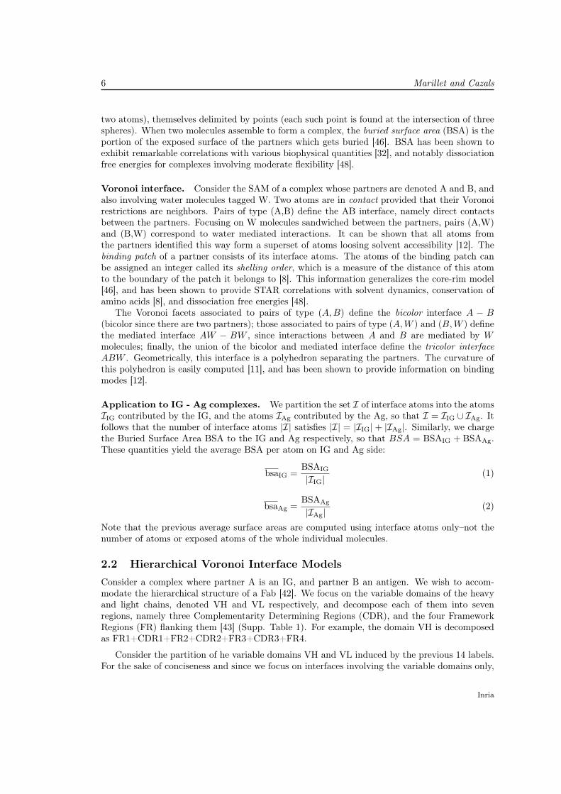
More formally, recall that the boundary of a surface accessible model (SAM, see Section 2.1)consists of spherical polygons, circle arcs, and points. For a given CDR, two sets of atoms are ofparticular interest, namely the atoms making up the boundary of the SAM and the subset of theseatoms which are found at the interface with the ligand. We note in passing that median valuesof the ratios between these two sets are 19%, 23%, 25%, for VH CDR1, VH CDR2, VH CDR3,respectively, and 18%, 10% and 24% for VL CDR1, VL CDR2 and VL CDR3, respectively.
Consider two CDR, and one set of atoms per CDR (either exposed atoms, or interfacial ex-posed atoms). The seam between these two sets of atoms is the contiguous set of circle arcsseparating these two sets of atoms, if any. Its length is defined as the cumulative length ofits constitutive circle arcs (Fig. 8). Practically, the seams associated with exposed and interfa-cial exposed atoms yield complementary pieces of information: the former describe the relativepositions of CDR; the latter provide information on the ligand position across these seams.
We computed the length of seams observed between all pairs of CDR on groups of complexesinvolving (i) the same ligand type, namely protein, peptide or chemical, and (ii) the same typeof VL domain, namely V-kappa or V-lambda. Denoting x and y two seam lengths, we define themaximum normalized difference as the following number ∈ [−100, 100]:
MND(x, y) = 100 · x− ymax(x, y)
. (3)
Given two CDR, we use the MND to compare the median value observed on a class of IG - Agcomplexes, against the median value observed over all complexes – this latter value being referred
Inria

Dissecting Interfaces of Antibody - Antigen Complexes 11
to as the consensus value or the value of the consensus seam. It is negative when the class-specificvalue is smaller than the consensus value, positive when it is greater and null if they are equal.
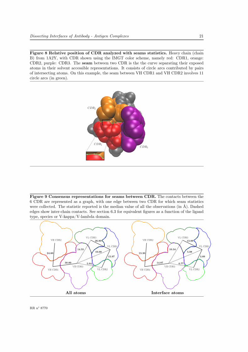
Consensus seams. We observe that the existing inter-chain contacts are the same when con-sidering either all atoms or interface atoms only (Fig. 9, supp. Figs. 19 and 20). Intuitively, theAg spreads evenly on the surface of the IG, covering all the seams.
Considering intra-chain contacts, we notice that the same are found in the VH and VLdomains, namely CDR1 – CDR2 and CDR1 – CDR3. However, considering all atoms, theseseams are slightly longer in VH with respectively 24.6 Å and 30.9 Å versus 16.0 Å and 26.9 Åfor VL. The same applies for interface atoms with 13.3 Å and 14.9 Å for the VH versus 3.9 Åand 13.9 Å for VL, respectively. This is likely because CDR from VH are longer on average thanthose from VL. Interestingly, the seams length is divided by approximately two when consideringonly interface atoms except for seam VL CDR1 – VL CDR2 where the it is divided by four.
For inter-chain contacts and considering all atoms, the length of the seam between VH CDR3and VL CDR3 is slightly smaller than, but comparable to, those existing intra-chain seams (14.5Å versus a median of 25.5 Å). The contacts VH CDR3 – VL CDR1 and VH CDR3 – VL CDR2are rather unexpected and are of length of 10.0 and 5.9 Å, respectively. For interface atoms, thelength of the seam between VH CDR3 and VL CDR3 is 10.3 Å versus a median across all othernonzero intra-chain seams of 12.6 Å.
Summarizing, the pattern of seams is the same either when considering all exposed CDRatoms, or only interface atoms. Moreover, VH CDR3 is the one making most contacts withother CDR, and VH CDR3 and VL CDR3 account for most of the inter-domain contacts.
Comparison between ligand types. We use the maximum normalized difference (Eq. 3)to compare the consensus seam length and those observed for specific ligand types. Whenconsidering seams for all the atoms, it is clearly seen that large values of MND have oppositesigns for proteins on the one hand, and peptides and chemicals on the other hand (Fig. 10), anobservation in line with the previously observed differences between ligand types. The relativelocations of the CDR are therefore different between ligand types. Intuitively, these differenceswitness pre-formed features of CDR that will accommodate a particular ligand type. Movingto seams between interface atoms only, a similar observation is also expected. This turns outto be the case, except for the seam VH CDR3–VL CDR1, for which larger values are observedfor peptides and chemicals (Fig. 10, left). In general, VL CDR1 shows differences opposite toVL CDR2 and VL CDR3 with respect to VH CDR3. This hints for a different role at the interfaceand potentially different dynamical properties.
Comparison between V-lambda and V-kappa domain. For all atoms, the largest lengthdifferences between V-kappa and V-lambda are found for the seams VH CDR1 – VH CDR2 (24.7versus 20.4 Å, Supp Fig. 27), VH CDR2 – VH CDR3 (0.0 versus 3.2 Å) and VH CDR3 – VL CDR1(9.4 versus 12.2 Å). Interestingly, two out of three are within VH and all involve VH CDR3. Forinterface atoms, the largest length differences between V-kappa and V-lambda are found for theseams VH CDR3 – VL CDR1 (5.6 versus 8.4 Å, Supp. Fig. 28), VL CDR1 – VL CDR3 (14.2versus 11.0 Å).
The V-kappa/V-lambda classification only pertaining to the light chain, it is sound to finddifferences in the relative positions of VL CDR1 and VL CDR3. Considering the differencesobserved for VH CDR, one has to recall that the pairing between heavy and light chains is acriterion during the selection of productive IG. It could be that IGLV and IGKV of light chainshave preferences for different sets of IGHV of heavy chains which would explain why looking
RR n° 8770

12 Marillet and Cazals
at IG with kappa light chains versus lambda light chains results in structural differences in theheavy chains.
3.4 Affinity prediction
As recalled in Introduction, estimating the affinity of an IG for an antigen is a challengingproblem, due in particular to the necessity to estimate the entropic penalty inherent to binding.In [50], we developed an affinity estimation strategy yielding state-of-the-art results, selectingsparse linear regressors defined from a pool of 12 variables aiming at modeling the enthalpicand entropic changes upon binding. Of particular interest are variables coding atomic packingproperties, and the position of atoms on binding patches, using their shelling order (Fig. 1 and[50]). To fit a model, we use the structure affinity benchmark (SAB) [34], a dataset containing144 cases, each case being described by three crystal structures (the unbound partners and thecomplex) and the experimentally measured binding affinity. Interestingly, the SAB contains 17IG - Ag cases 1. We therefore trained the general model from [50] using the 139 − 14 cases, topredict the affinities of the selected 14 IG - Ag cases. We note in passing that the iRMSD andthe total RMSD between the bound and unbound form of the IG are always smaller than 1.24 Åand 0.95Å respectively. That is, the 14 cases are essentially rigid body docking cases, a propertywhich, however, does not warrant easiness of binding affinity prediction [50].
Upon performing the affinity prediction, our model predicts 9 (64.29 %), 13 (92.86 %) and14 (100 %) of the Kd within one, two and three orders of magnitude respectively, with a medianabsolute error of 1.024 kcal/mol (Supp. Fig. 31). From an absolute affinity prediction error,these results are satisfactory, as predicting Kd within one order of magnitude is essentially thebest one can hope for without modeling subtle effects such as the pH in particular [31]. Froma relative standpoint, they are also informative, as an affinity enhancement of two orders ofmagnitude is typically observed during affinity maturation [60].
4 Discussion
This paper presents a comprehensive analysis of IG - Ag complexes and their interfaces, basedon state-of-the-art modeling tools relying upon hierarchical Voronoi interface models and relatedgeometric constructions. Our dissection of IG - Ag interfaces yields a number of novel insights,which may be summarized by considering the whole interface level and the CDR level.
Global interface statistics. While a classical focus in previous work has been the classifi-cation of backbone conformations, an endeavor boiling down to comparing backbone traces, wefocus instead on interfacial atoms, as identified by a solvent accessible model. In doing so, oneobserves that side chains contribute approximately twice as many atoms than backbones. Whilethis statistic stresses the need to consider all interface atoms rather than backbone ones only,modeling side chains accurately enough to encompass their incidence on binding thermodynamicand kinetic properties is extremely challenging, due in particular to correlations between ro-tameric states of side-chains. The length of CDR3 also raises difficulties, and as an extreme case,one may consider exceptionally long VH CDR3, such as thos found in bovine antibodies, wheremultiple cysteines facilitate the formation of disulfide bonds and microfolds [71, 7].
1 (PDB IDs: 1AHW, 1BJ1, 1BVK, 1DQJ, 1E6J, 1FSK, 1IQD, 1JPS, 1MLC, 1NCA, 1NSN, 1P2C, 1VFB,1WEJ, 2JEL, 2VIR and 2VIS). However, 1IQD and 1NSN are discarded as only an upper bound on their Kd isprovided in the SAB. Furthermore, 1E6J is also discarded because too many atoms could not be matched betweenthe bound and unbound structures.
Inria

Dissecting Interfaces of Antibody - Antigen Complexes 13
Additionally, the simplest and most informative variable describing protein interfaces beingthe buried surface area (BSA), we refine this statistic by computing the average BSA contributedby interfacial atoms from the IG (statistic bsaIG) and the Ag (statistic bsaAg). These quantitiesturn out to be clear signatures of the ligand type, a property which can further be exploited forclassification purposes. While the classification of IG - Ag interfaces into classes depending onstructural features has already been addressed [14, 40], our parameters are the first ones yieldingsuch a clear separation between specific antigen types.
Contributions of CDR. In considering IG - Ag interfaces, it is generally believed thatVH CDR3 plays a prominent role [73] and is the most variable, a property owing to the ge-netic V(D)J rearrangement mechanisms underlying its formation and that it is the one withdominant contribution to the Ag binding. To refine this view, our goal has been to preciselycharacterize the respective contributions of CDR at interfaces, and the relative positions of thesix CDR along with the ligand position across them.
For the roles of all CDRs, while we confirm the prominent role of VH CDR3, we also observethat in terms of buried surface area, the contribution of VH CDR3 is essentially matched by thejoint contributions of VH CDR1 and VH CDR2. Thus, in terms of binding affinity and whilefocusing on the interaction energy between the IG and the Ag, a precise description needs toconsider VH CDR3 and VH CDR1 + VH CDR2 on an equal footing. The BSA has long beenknown as a simple and informative descriptor of interfaces [4], and we show that the average BSAper atom is a signature of the ligand type bound by an IG. Since we also show that the lengthof CDR does not correlate with their BSA, we suggests that despite the statistical significanceof correlations between CDR length and ligand type [21], predicting the ligand type bound byan IG requires more than only CDR length information. Moreover the fact that CDR of thesame length can have radically different contribution at the interface, calls into question theclassification of CDR into canonical structures based on individual CDR lengths [54]. Finally,we also note that VL CDR2 hardly contributes to the interface for chemical ligands, and verylittle in general.
As far as the relative position of CDR is concerned, a precise characterization was missingto complement qualitative views [20, Chapter 4]. We fill this gap analyzing seam statistics,namely contiguous boundaries between pairs of CDR, for all CDR atoms, and also for interfacialCDR atoms. Remarkably, out of 15 possibles seams, only seven appear, and these are remarkablyconserved–irrespective of the ligand type or the category of atoms considered. Phrased differently,the same seams occur within VH and VL, but they are longer in VH. Several other remarkablefacts emerge from this analysis. First, the arrangement of CDR are more similar between peptideand chemical ligands than between peptide or chemical ligands and protein ligands. In a similarvein, the seam between VL CDR1 and VL CDR2 contributes more to the interface for proteinligands than for peptide or chemical ligands. These features specifically identify the ligandtargeted, a property complementing the observations already made at the whole interface level.Second, VL CDR2 is often away from the interface.
We finally note that our approach favors a purely geometric description of the IG and theIG - Ag complex structures, and that, as such, it complements the numerous analyses focusedon CDR amino acid composition and length based on sequence data [61, 30, 26, 19] [6, 67, 5].
Affinity prediction. To complement the previous analysis, we applied recent binding affinitypredictors based on the same structural parameters [50] so as to predict the binding affinity of14 IG with their respective Ag. These are all rigid cases as the interface RMSD and whole IGRMSD were below 1.24 and 0.95 Å, respectively. The predictions of Kd are accurate within twoorders of magnitude for all but one complex and within one order of magnitude for 9 of them.
RR n° 8770

14 Marillet and Cazals
Although they were obtained on a very small dataset, these results suggest that predictions atthis level of accuracy for IG may be easier than for more general protein - protein complexes[50].
However, obtaining more accurate predictions, say within one order of magnitude or equiva-lently within 1.4 kcal/mol remains an open problem, as taking subtle entropic effects coding thedynamics appears mandatory [60].
Future work. This work proposes novel parameters shedding light on the specificity of IG fortheir antigens, and the binding affinity of the corresponding complexes. Outstanding questionsremain, both to model interfaces of IG - Ag complexes, and to model whole IG.
At the interface level, predicting the geometry of a complex given the unbound partners, andthe associated affinity remains a daunting challenge. The classical route consists of using samplingtechniques and docking algorithms to generate poses for the complex, which are further rankedby scoring functions aiming at detecting the most plausible ones. Our work bears promises in thispipeline, as our structural parameters (in particular the BSA per atom and the seam patterns)may be used to check that the complex selected matches the specific observations raised, inparticular as a function of the ligand type. Likewise, upon generating a valid geometry, ouraffinity prediction tools can be used to predict the affinity–a strategy calling again for tests onmore cases. Together, these tools could lead to consequent advances in antibody design [45, 63].
At the whole IG level, various structural features of IG proteins influence their propertieswhence their efficacy in the immune response. These include the ball-and-socket joint relatingVL and VH, the CL and CH1 constant domains [44, 66], and more generally the constant regionswhich have been shown to influence the avidity [22, 23, 51, 57], and are involved in IG effectorproperties, such as ADCC or CDC [29]. A quantitative assessment of the role of these featuresrequires going beyond the IG - Ag interface level, with a clear focus on the dynamics of the wholeIG protein. In doing so, novel ideas will be needed to sample efficiently conformations of wholeIG, and study the associated (potential, free) energy landscapes.
Inria

Dissecting Interfaces of Antibody - Antigen Complexes 15
RR n° 8770

16 Marillet and Cazals
5 Artwork
Figure 1 Voronoi interface model of an Immunoglobulin - Antigen (IG - Ag) com-plex, defined from the solvent accessible model of the crystallographic complex. TheIG consists of H and L chains, with here the VH and VL domains shown in grey (cartoon repre-sentation), while the Ag consists of the chain in blue (CPK representation). (Top left) IG - Agcomplex, with the six complementarity determining regions (CDR) colored using the IMGT con-ventions (VH CDR1: red, VH CDR2: orange, VH CDR3: purple, VL CDR1: blue, VL CDR2:green, VL CDR3: green-blue). (Top right) The Voronoi interface is a polyedral model separat-ing the partners, whose parameters (area, curvature) convey information of the binding modes.(Bottom left) The Voronoi interface can be divided into concentric shell. Each shell containsthe Voronoi facets which are at the same minimum distance from the interface boundary. Thisdistance is called the shelling order of the facet (SO for short). For instance, purple facets touchthe boundary (SO=1), blue facets must cross a purple facet to reach the boundary (SO=2),and so on. (Bottom right) Each face of the Voronoi interface involves two interacting atoms,either from the partners or the interfacial water molecules sandwiched between them. The buriedsurface area (BSA) on each partner (by the second partner and interfacial water) is of prime in-terest to describe the interface. For the IG, the BSA can be charged to the CDR and frameworkregions (FR). (Bottom right inset) The interface atoms of a partner define its binding patch,and, similarly to the Voronoi interface, can be shelled into concentric shells (from the outside tothe core), defining a distance to the patch boundary. The binding patch on the IG side is shownfrom above (inset) to get a clearer view of all the shells.
Inria

Dissecting Interfaces of Antibody - Antigen Complexes 17
Figure 2 Hierarchical decomposition of the Voronoi interface of Fig. 1. The IG (orthe Fab fragment) is decomposed into heavy (H) and light (L) chains (one H and one L perFab) whose variable domains only (VH and VL) are of interest in this study. These domains arefurther decomposed into three complementarity determining regions (CDR) and four frameworkregions (FR). These fourteen primitive labels induce a partition of the Voronoi interface andbinding patches.
IG Ag
IG-Ag complex Hierarchical decomposition
W
Partners: IG and Ag
IG
W
Ag
H
L LV H V L
V H
V L
Interfacialwater molecules
CDR1
CDR2
CDR3
FR1
FR2
FR3
FR4
CDR1
CDR2
CDR3
FR1
FR2
FR3
FR4
Fab
Figure 3 Average buried surface areas per atom (Equations (1) (2)): bsaIG versusbsaAg. (Main panel) Scatter plot as a function of the ligand type. The three lines show theseparators defined by the decision tree rules, separating the ligand types (see main text andSupp. Fig. 14). (Inset) Color gradient indicating the ligand size, in number of atoms, fromsmall (yellow) to large (red).
2 4 6 8 10BSA per atom, IG binding patch
5
10
15
20
25
30
35
40
45
BSA
per
ato
m, A
g b
indin
g p
atc
h
Chemical
Protein
Peptide2O5X
L1
L2
L3
RR n° 8770

18 Marillet and Cazals
Figure 4 Buried Surface Area (A2): relative contributions of the VH and VL.
0 200 400 600 800 1000 1200 1400 1600 1800BSA of VH
0
100
200
300
400
500
600
700
BS
A o
f V
L
Peptide
Protein
Chemical
x = y
3NGB
4OGY
Figure 5 Buried Surface Area (A2): relative contributions of the CDR.
0 100 200 300 400 500 600
CDR1 + CDR2 BSA (2
)
0
100
200
300
400
500
600
700
CD
R3
BSA
(2
)
VHPeptide
Protein
Chemical
x = y
(a) Relative contributions of the CDR from VH.
0 50 100 150 200 250 300 350 400
CDR1 + CDR2 BSA (2
)
0
50
100
150
200
250
300
CD
R3
BSA
(2
)
VLPeptide
Protein
Chemical
x = y
(b) Relative contributions of the CDR from VL
Inria

Dissecting Interfaces of Antibody - Antigen Complexes 19
Figure 6 VH CDR length versus BSA. VH CDR1 and VH CDR2 are grouped due to theircommon genomic origin.
0 100 200 300 400 500 600
BSA(CDR1) + BSA(CDR2) (2
)
[8, 7]
[8, 8]
[8, 10]
[9, 7]
[10, 7]
[10, 9]
Length
of
[CD
R1
, C
DR
2]
in A
A
Chemical
Protein
Peptide
(a) VH CDR1 and VH CDR2, Human. Five com-plexes are discarded because of aberrant VH CDR1and VH CDR2 lengths (see Supp. Section 6.2).
0 100 200 300 400 500
BSA(CDR1) + BSA(CDR2) (2
)
[8, 7]
[8, 8]
[8, 10]
[9, 7]
[10, 7]
Length
of
[CD
R1
, C
DR
2]
in A
A
Chemical
Protein
Peptide
(b) VH CDR1 and VH CDR2, Mouse.
0 100 200 300 400 500 600 700
BSA (2
)
5
10
15
20
25
Length
in A
A
Chemical
Protein
Peptide
(c) VH CDR3, Human. Twelve complexes are dis-carded because of aberrant VL CDR1 and VL CDR2lengths (see Supp. Section 6.2).
0 100 200 300 400 500
BSA (2
)
4
6
8
10
12
14
16
18
20
Length
in A
A
Chemical
Protein
Peptide
(d) VH CDR3, Mouse.
RR n° 8770

20 Marillet and Cazals
Figure 7 VL CDR length versus BSA. VL CDR1 and VL CDR2 are grouped due to theircommon genomic origin.
0 50 100 150 200 250 300 350
BSA(CDR1) + BSA(CDR2) (2
)
[6, 3]
[7, 3]
[8, 3]
[9, 3]
[11, 3]
[12, 3]
Length
of
[CD
R1
, C
DR
2]
in A
A
Chemical
Protein
Peptide
(a) VL CDR1 and VL CDR2, Human. The[CDR1.CDR2] lengths [6.3] characterize both V-kappa and V-lambda. The other lengths charac-terize either V-kappa ([7.3], [11.3] and [12.3]) or V-lambda ([8.3] and [9.3]).
0 50 100 150 200 250 300 350 400
BSA(CDR1) + BSA(CDR2) (2
)
[5, 3]
[6, 3]
[7, 3]
[7, 7]
[9, 3]
[10, 3]
[11, 3]
[12, 3]
Length
of
[CD
R1
, C
DR
2]
in A
A
Chemical
Protein
Peptide
(b) VL CDR1 and VL CDR2, Mouse. The[CDR1.CDR2] lengths [7.7] and [9.3] characterize V-lambda. The other lengths characterize V-kappa.
0 50 100 150 200 250 300
BSA (2
)
4
6
8
10
12
14
16
18
20
Length
in A
A
Chemical
Protein
Peptide
(c) VL CDR3, Human.
0 50 100 150 200 250 300
BSA (2
)
8
9
10
11
12
13
Length
in A
A
Chemical
Protein
Peptide
(d) VL CDR3, Mouse.
Inria
Dissecting Interfaces of Antibody - Antigen Complexes 21
Figure 8 Relative position of CDR analyzed with seams statistics. Heavy chain (chainB) from 1A2Y, with CDR shown using the IMGT color scheme, namely red: CDR1, orange:CDR2, purple: CDR3. The seam between two CDR is the the curve separating their exposedatoms in their solvent accessible representations. It consists of circle arcs contributed by pairsof intersecting atoms. On this example, the seam between VH CDR1 and VH CDR2 involves 11circle arcs (in green).
CDR1
CDR2
CDR3
Figure 9 Consensus representations for seams between CDR. The contacts between the6 CDR are represented as a graph, with one edge between two CDR for which seam statisticswere collected. The statistic reported is the median value of all the observations (in Å). Dashededges show inter-chain contacts. See section 6.3 for equivalent figures as a function of the ligandtype, species or V-kappa/V-lambda domain.
VH CDR2
VH CDR1VH CDR3
VL CDR3
VL CDR1
VL CDR2
24.60
30.89
14.5510.00
5.94
26.89
15.97
VH CDR2
VH CDR1VH CDR3
VL CDR3
VL CDR1
VL CDR2
13.30
14.87
10.345.98
0.77
13.88
3.89
All atoms Interface atoms
RR n° 8770

22 Marillet and Cazals
Figure 10 Comparison between the consensus median seam lengths and the medianlengths for specific ligand types. The y axis represents the maximum normalized difference(Eq. (3)) between the consensus median length and the median length for specific ligand types.Filled bars correspond to inter-chain contacts. Note that for a given ligand type, there are 7 barscorresponding to the pairs of CDR in contact.
protein peptide chemical
Max
imum
nor
mal
ized
diff
eren
ce
−20
−12
−8
−4
04
812
1620
24
VH CDR1−VH CDR2VH CDR1−VH CDR3VH CDR3−VL CDR1VH CDR3−VL CDR2VH CDR3−VL CDR3VL CDR1−VL CDR2VL CDR1−VL CDR3
protein peptide chemical
Max
imum
nor
mal
ized
diff
eren
ce
−10
0−
75−
45−
150
1530
4560
75
VH CDR1−VH CDR2VH CDR1−VH CDR3VH CDR3−VL CDR1VH CDR3−VL CDR2VH CDR3−VL CDR3VL CDR1−VL CDR2VL CDR1−VL CDR3
All atoms Interface atoms
Acknowledgements. Patrice Duroux is acknowledged for his help with the IMGT/3Dstructure-DB database.
References
[1] A. Ademokun, Y-C. Wu, V. Martin, R. Mitra, U. Sack, H. Baxendale, D. Kipling, and D.K.Dunn-Walters. Vaccination-induced changes in human b-cell repertoire and pneumococcaligm and iga antibody at different ages. Aging cell, 10(6):922–930, 2011.
[2] B. Al-Lazikani, A.M. Lesk, and C. Chothia. Standard conformations for the canonicalstructures of immunoglobulins. Journal of molecular biology, 273(4):927–948, 1997.
[3] J.C Almagro. Identification of differences in the specificity-determining residues of antibodiesthat recognize antigens of different size: implications for the rational design of antibodyrepertoires. Journal of Molecular Recognition, 17(2):132–143, 2004.
[4] R. Bahadur, P. Chakrabarti, F. Rodier, and J. Janin. A dissection of specific and non-specificprotein–protein interfaces. JMB, 336(4):943–955, 2004.
[5] J. Benichou, J. Glanville, E.T. Luning Prak, R. Azran, T.C. Kuo, J. Pons, C. Desmarais,L. Tsaban, and Y. Louzoun. The restricted DH gene reading frame usage in the expressedhuman antibody repertoire is selected based upon its amino acid content. The Journal ofImmunology, 190(11):5567–5577, 2013.
Inria

Dissecting Interfaces of Antibody - Antigen Complexes 23
[6] S. Birtalan, Y. Zhang, F.A. Fellouse, L. Shao, G. Schaefer, and S.S. Sidhu. The intrin-sic contributions of tyrosine, serine, glycine and arginine to the affinity and specificity ofantibodies. Journal of molecular biology, 377(5):1518–1528, 2008.
[7] Y. Bordon. Cow traps are structurally unique. Nature Reviews Immunology, 13(471), 2013.
[8] B. Bouvier, R. Grunberg, M. Nilgès, and F. Cazals. Shelling the Voronoi interface ofprotein-protein complexes reveals patterns of residue conservation, dynamics and composi-tion. Proteins: structure, function, and bioinformatics, 76(3):677–692, 2009.
[9] J.D. Capra and J.M. Kehoe. Hypervariable regions, idiotypy, and the antibody-combiningsite. Adv. Immunol, 20(1), 1975.
[10] R. Castro, L. Journeau, H.P. Pham, O. Bouchez, V. Giudicelli, M-P. Lefranc, E. Quillet,A. Benmansour, F. Cazals, A. Six, S. Fillatreau, O. Sunyer, and P. Boudinot. Teleost fishmount complex clonal IgM and IgT responses in spleen upon systemic viral infection. PLOSPathogens, 9(1):e1003098, 2013.
[11] F. Cazals. Revisiting the Voronoi description of protein-protein interfaces: Algorithms. InT. Dijkstra, E. Tsivtsivadze, E. Marchiori, and T. Heskes, editors, International Conferenceon Pattern Recognition in Bioinformatics, pages 419–430, Nijmegen, the Netherlands, 2010.Lecture Notes in Bioinformatics 6282.
[12] F. Cazals, F. Proust, R. Bahadur, and J. Janin. Revisiting the Voronoi description ofprotein-protein interfaces. Protein Science, 15(9):2082–2092, 2006.
[13] A. Chailyan, P. Marcatili, D. Cirillo, and A. Tramontano. Structural repertoire of im-munoglobulin λ light chains. Proteins: Structure, Function, and Bioinformatics, 79(5):1513–1524, 2011.
[14] A. Chailyan, P. Marcatili, and A. Tramontano. The association of heavy and lightchain variable domains in antibodies: implications for antigen specificity. FEBS Journal,278(16):2858–2866, 2011.
[15] C.A. Chia-en, W. Chen, and M.K. Gilson. Ligand configurational entropy and proteinbinding. PNAS, 104(5):1534–1539, 2007.
[16] Y. Choi and C.M. Deane. Predicting antibody complementarity determining region struc-tures without classification. Molecular Biosystems, 7(12):3327–3334, 2011.
[17] C. Chothia and A.M. Lesk. Canonical structures for the hypervariable regions of im-munoglobulins. J. Mol. Bio, 196(4), 1987.
[18] C. Chothia, A.M. Lesk, A. Tramontano, M. Levitt, S.J. Smith-Gill, G. Air, S. Sheriff, E.A.Padlan, D. Davies, W.R. Tulip, et al. Conformations of immunoglobulin hypervariableregions. Nature, 342(6252):877–883, 1989.
[19] L.A. Clark, S. Ganesan, S. Papp, and H.W.T van Vlijmen. Trends in antibody sequencechanges during the somatic hypermutation process. The Journal of Immunology, 177(1):333–340, 2006.
[20] R. Coico and G. Sunshine. Immunology: a short course. John Wiley & Sons, 2009.
RR n° 8770

24 Marillet and Cazals
[21] A.V.J. Collis, A.P. Brouwer, and A.C.R. Martin. Analysis of the antigen combining site:correlations between length and sequence composition of the hypervariable loops and thenature of the antigen. Journal of molecular biology, 325(2):337–354, 2003.
[22] L.J. Cooper, A.R. Shikhman, D.D Glass, D. Kangisser, M.W. Cunningham, and N.S.Greenspan. Role of heavy chain constant domains in antibody-antigen interaction. appar-ent specificity differences among streptococcal IgG antibodies expressing identical variabledomains. The Journal of Immunology, 150(6):2231–2242, 1993.
[23] L.J.N Cooper, D. Robertson, R. Granzow, and N.S. Greenspan. Variable domain-identicalantibodies exhibit IgG subclass-related differences in affinity and kinetic constants as deter-mined by surface plasmon resonance. Molecular immunology, 31(8):577–584, 1994.
[24] J. Dunitz. Win some, lose some: enthalpy-entropy compensation in weak intermolecularinteractions. Chemistry & biology, 2(11):709–712, 1995.
[25] F. Ehrenmann, Q. Kaas, and M-P. Lefranc. IMGT/3Dstructure-DB andIMGT/DomainGapAlign: a database and a tool for immunoglobulins or antibodies,T cell receptors, MHC, IgSF and MhcSF. Nucl. Acids Res., 38:D301–307, 2010.
[26] F.A. Fellouse, P.A. Barthelemy, R.F. Kelley, and S.S. Sidhu. Tyrosine plays a dominantfunctional role in the paratope of a synthetic antibody derived from a four amino acid code.Journal of molecular biology, 357(1):100–114, 2006.
[27] W.J.J Finlay and J.C. Almagro. Natural and man-made v-gene repertoires for antibodydiscovery. Frontiers in immunology, 3, 2012.
[28] M. Gerstein and F.M. Richards. Protein geometry: volumes, areas, and distances. In M. G.Rossmann and E. Arnold, editors, The international tables for crystallography (Vol F, Chap.22), pages 531–539. Springer, 2001.
[29] L.W. Guddat, L. Shan, Z-C. Fan, K.N. Andersen, R. Rosauer, D.S. Linthicum, and A.B.Edmundson. Intramolecular signaling upon complexation. The FASEB journal, 9(1):101–106, 1995.
[30] I. Ivanov, J-M. Link, G. Ippolito, and H.H. Schroeder. Constraints on hydropathicity andsequence composition of HCDR3 are conserved across evolution. The antibodies, 7:43–67,2002.
[31] J. Janin. A minimal model of protein–protein binding affinities. Protein Science,23(12):1813–1817, 2014.
[32] J. Janin, R. P. Bahadur, and P. Chakrabarti. Protein-protein interaction and quaternarystructure. Quarterly reviews of biophysics, 41(2):133–180, 2008.
[33] S. Jones and JM Thornton. Principles of protein-protein interactions. PNAS, 93(1):13–20,1996.
[34] P.L. Kastritis, I.H. Moal, H. Hwang, Z. Weng, P.A. Bates, A. Bonvin, and J. Janin. Astructure-based benchmark for protein-protein binding affinity. Protein Science, 20:482–491, 2011.
[35] P.L. Kastritis, J.P.G.L.M. Rodrigues, G.E. Folkers, R. Boelens, and A.M.J.J. Bonvin. Pro-teins feel more than they see: Fine-tuning of binding affinity by properties of the non-interacting surface. J.M.B., 426:2632–2652, 2014.
Inria

Dissecting Interfaces of Antibody - Antigen Complexes 25
[36] O.V. Koliasnikov, M.O. Kiral, V.G. Grigorenko, and A.M. Egorov. Antibody CDR H3modeling rules: extension for the case of absence of Arg H94 and Asp H101. Journal ofbioinformatics and computational biology, 4(02):415–424, 2006.
[37] D. Kuroda, H. Shirai, M. Kobori, and H. Nakamura. Structural classification of CDR-H3revisited: A lesson in antibody modeling. Proteins: Structure, Function, and Bioinformatics,73(3):608–620, 2008.
[38] D. Kuroda, H. Shirai, M. Kobori, and H. Nakamura. Systematic classification of CDR-L3in antibodies: Implications of the light chain subtypes and the VL–VH interface. Proteins:Structure, Function, and Bioinformatics, 75(1):139–146, 2009.
[39] N.F. Landolfi, A.B. Thakur, H. Fu, M. Vásquez, C. Queen, and N. Tsurushita. The integrityof the ball-and-socket joint between V and C domains is essential for complete activity of ahumanized antibody. The Journal of Immunology, 166(3):1748–1754, 2001.
[40] M. Lee, P. Lloyd, X. Zhang, J.M. Schallhorn, K. Sugimoto, A.G. Leach, G. Sapiro, andK.N. Houk. Shapes of antibody binding sites: qualitative and quantitative analyses basedon a geomorphic classification scheme. The Journal of organic chemistry, 71(14):5082–5092,2006.
[41] M-P. Lefranc. Immunoglobulin (IG) and T cell receptor (TR) genes: IMGT® and the birthand rise of immunoinformatics. Frontiers in Immunology, 5:22, 2014.
[42] M-P. Lefranc and G. Lefranc. The immunoglobulin FactsBook. Academic Press, 2001.
[43] M-P. Lefranc, C. Pommié, M. Ruiz, V. Giudicelli, E. Foulquier, L. Truong, V. Thouvenin-Contet, and G. Lefranc. IMGT unique numbering for immunoglobulin and T cell receptorvariable domains and Ig superfamily V-like domains. Developmental & Comparative Im-munology, 27(1):55–77, 2003.
[44] A. Lesk and C. Chothia. Elbow motion in the immunoglobulins involves a molecular ball-and-socket joint. Nature, 8(335):188–90, 1988.
[45] S.M. Lippow, K.D. Wittrup, and B. Tidor. Computational design of antibody-affinity im-provement beyond in vivo maturation. Nature biotechnology, 25(10):1171–1176, 2007.
[46] L. Lo Conte, C. Chothia, and J. Janin. The atomic structure of protein-protein recognitionsites. JMB, 285(5):2177–2198, 1999.
[47] R.M. MacCallum, A.C.R. Martin, and J.M. Thornton. Antibody-antigen interactions: con-tact analysis and binding site topography. Journal of molecular biology, 262(5):732–745,1996.
[48] N. Malod-Dognin, A. Bansal, and F. Cazals. Characterizing the morphology of proteinbinding patches. Proteins: structure, function, and bioinformatics, 80(12):2652–2665, 2012.
[49] V. Manivel, N.C. Sahoo, D.M. Salunke, and K.V.S Rao. Maturation of an antibody responseis governed by modulations in flexibility of the antigen-combining site. Immunity, 13(5):611–620, 2000.
[50] S. Marillet, P. Boudinot, and F. Cazals. High resolution crystal structures leverage proteinbinding affinity predictions. Under revision, (NA), 2015. Preprint: Inria tech report 8733.
RR n° 8770

26 Marillet and Cazals
[51] N McCloskey, MW Turner, P Steffner, R Owens, and D Goldblatt. Human constant regionsinfluence the antibody binding characteristics of mouse-human chimeric IgG subclasses.Immunology, 88(2):169–173, 1996.
[52] G. Meng, N. Arkus, M.P. Brenner, and V.N. Manoharan. The free-energy landscape ofclusters of attractive hard spheres. Science, 327(5965):560–563, 2010.
[53] V. Morea, A. Tramontano, M. Rustici, C. Chothia, and A.M. Lesk. Conformations of thethird hypervariable region in the VH domain of immunoglobulins. Journal of molecularbiology, 275(2):269–294, 1998.
[54] B. North, A. Lehmann, and R.L. Dunbrack. A new clustering of antibody CDR loopconformations. Journal of molecular biology, 406(2):228–256, 2011.
[55] W.E. Paul. Fundamental Immunology (7th Ed.). Lippincott Williams and Wilkins, Woltersand Kluwer, 2013.
[56] O. Pritsch, G. Hudry-Clergeon, M. Buckle, Y. Pétillot, J-P. Bouvet, J. Gagnon, andG. Dighiero. Can immunoglobulin CH1 constant region domain modulate antigen bind-ing affinity of antibodies? Journal of Clinical Investigation, 98(10):2235, 1996.
[57] O. Pritsch, C. Magnac, G. Dumas, J-P. Bouvet, P. Alzari, and G. Dighiero. Can isotypeswitch modulate antigen-binding affinity and influence clonal selection? European journalof immunology, 30(12):3387–3395, 2000.
[58] G. Raghunathan, J. Smart, J. Williams, and J-C. Almagro. Antigen-binding site anatomyand somatic mutations in antibodies that recognize different types of antigens. Journal ofMolecular Recognition, 25(3):103–113, 2012.
[59] D. Rajamani, S. Thiel, S. Vajda, and C.J. Camacho. Anchor residues in protein-proteininteractions. PNAS, 101(31):11287–11292, 2004.
[60] A. Schmidt, H. Xu, A. Khan, T. O’Donnell, S. Khurana, L. King, J. Manischewitz, H. Gold-ing, P. Suphaphiphat, A. Carfi, E. Settembre, P. Dormitzer, T. Kepler, R. Zhang, A. Moody,B. Haynes, H-X. Liao, D. Shaw, and S. Harrison. Preconfiguration of the antigen-bindingsite during affinity maturation of a broadly neutralizing influenza virus antibody. PNAS,110(1):264–269, 2013.
[61] H.W. Schroeder, M. Zemlin, M. Khass, H.H. Nguyen, and R.L. Schelonka. Genetic controlof DH reading frame and its effect of B-cell development and antigen-specific antibodyproduction. Critical reviews in Immunology, 30(4):327–344, 2010.
[62] H. Shirai, A. Kidera, and H. Nakamura. Structural classification of CDR-H3 in antibodies.FEBS letters, 399(1):1–8, 1996.
[63] H. Shirai, C. Prades, R. Vita, P. Marcatili, B. Popovic, J. Xu, J.P. Overington, K. Hirayama,S. Soga, K. Tsunoyama, et al. Antibody informatics for drug discovery. Biochimica etBiophysica Acta (BBA)-Proteins and Proteomics, 1844(11):2002–2015, 2014.
[64] J. Shirai, A. Kidera, and H. Nakamura. H3-rules: identification of CDR-H3 structures inantibodies. FEBS letters, 455(1):188–197, 1999.
Inria

Dissecting Interfaces of Antibody - Antigen Complexes 27
[65] A. Six, M.E. Mariotti-Ferrandiz, W. Chaara, S. Magadan, H-P. Pham, M-P. Lefranc,T. Mora, V. Thomas-Vaslin, A.M. Walczak, and P.Boudinot. The past, present, and futureof immune repertoire biology–the rise of next-generation repertoire analysis. Frontiers inimmunology, 4, 2013.
[66] R.L. Stanfield, A. Zemla, I.A Wilson, and B. Rupp. Antibody elbow angles are influencedby their light chain class. Journal of molecular biology, 357(5):1566–1574, 2006.
[67] C.A. Thomson, K.Q. Little, D.C. Reason, and J.W. Schrader. Somatic diversity in CDR3loops allows single V-genes to encode innate immunological memories for multiple pathogens.The Journal of Immunology, 186(4):2291–2298, 2011.
[68] S. Tonegawa. Somatic generation of antibody diversity. Nature, 302(5909):575–581, 1983.
[69] M. Torres, N. Fernández-Fuentes, A. Fiser, and A. Casadevall. The immunoglobulin heavychain constant region affects kinetic and thermodynamic parameters of antibody variableregion interactions with antigen. Journal of Biological Chemistry, 282(18):13917–13927,2007.
[70] E. Vargas-Madrazo, F. Lara-Ochoa, and J.C. Almagro. Canonical structure repertoire of theantigen-binding site of immunoglobulins suggests strong geometrical restrictions associatedto the mechanism of immune recognition. Journal of molecular biology, 254(3):497–504,1995.
[71] F. Wang, D.C. Ekiert, I. Ahmad, W. Yu, Y. Zhang, O. Bazirgan, A. Torkamani, T. Raud-sepp, W. Mwangi, M.F. Criscitiello, et al. Reshaping antibody diversity. Cell, 153(6):1379–1393, 2013.
[72] T.T. Wu and E.A. Kabat. An analysis of the sequences of the variable regions of bence jonesproteins and myeloma light chains and their implications for antibody complementarity. TheJournal of experimental medicine, 132(2):211–250, 1970.
[73] J.L Xu and M.M. Davis. Diversity in the CDR3 region of VH is sufficient for most antibodyspecificities. Immunity, 13(1):37–45, 2000.
RR n° 8770

28 Marillet and Cazals
6 Supplemental: Results
6.1 Dataset
We use the IMGT/3Dstructure-DB database [25], version of January 2015. For each entry, theatoms of the complementarity determining regions (CDR) of the IG are annotated using theIMGT unique numbering scheme [43], recalled in Table 1. Out of 1363 submitted files, 1035 wereprocessed (other were discarded because of various problems, see the report in appendix), 596complexes were extracted after the redundancy was filtered, out of which 537 could be part ofthe analysis (26 other were discarded because there was no interface or the contacts were notmade with the Fab of the IG)
Table 1 Amino acid positions associated with each IMGT label defining the decom-position of a V-domain into seven regions Positions of the complementarity determiningregions (CDR) using the IMGT numbering scheme [43].
Region FR1 CDR1 FR2 CDR2 FR3 CDR3 FR4start-stop 1 - 26 27 - 38 39 - 55 56 - 65 66 - 104 105 - 117 118 - 128
Table 2 Summary of the number of IG - Ag complexes in each class of species / ligandtype. The dataset includes VH (V-domains of heavy chains)and VL comprisingV-KAPPA (V domains of kappa chains) and V-LAMBDA (V domains of lambdachains.
Mouse Human Other totalPeptide 81 34 11 126Protein 191 104 31 326Chemical 65 7 5 77total 337 145 47 529
Table 3 Number of occurrences of the isotypes in the datasetIsotype A G M UnknownNumber of occurrences 1 484 0 44
Inria

Dissecting Interfaces of Antibody - Antigen Complexes 29
Table 4 V-domains of the IG – Ag complexes are assigned to the respective sub-groups: VH to the IGHV subgroups, V-kappa to the IGKV subgroups and V-lambdato the IGLV subgroups. The number (Nb) of functional (F) genes per IGHV, IGKV and IGLVsubgroup in human (Homo sapiens) and the CDR1 and CDR2 lengths [CDR1.CDR2.] of thegermline genes are from IMGT Protein displays. Eight complexes were annotated with aberrantCDR lengths considering their IGH subgroup, twelve considering their IGK subgroups, and oneconsidering its IGL subgroup. They were not counted in this table.
HumanIGHV subgroups and genes IGKV subgroups and genes IGLV subgroups and genes
Subgroup [CDR1.CDR2] NB F VH Subgroup [CDR1.
CDR2] NB F V-kappa Subgroup [CDR1.CDR2] NB F V-lambda
IGHV1 [8.8] 11 36 IGKV1 [6.3] 19 58 IGLV1 [8.3] 4 27[9.3] 1 0
IGHV2 [10.7] 3 3 IGKV2 [11.3] 7 3 IGLV2 [9.3] 5 3[12.3] 2 0
IGHV3 [8.8] 16 60 IGKV3 [6.3] 4 8 IGLV3 [6.3] 10 13[8.7] 3 2 [7.3] 3 14[8.10] 4 5
IGHV4 [9.7] 3 2 IGKV4 [12.3] 1 3 IGLV4 [7.7] 3 0[8.7] 2 10[10.7] 5 2
IGHV5 [8.8] 2 12 IGKV5 [6.3] 1 0 IGLV5 [9.7] 4 0IGHV6 [10.9] 1 2 IGKV6 [6.3] 2 0 IGLV6 [8.3] 1 2IGHV7 [8.8] 1 3 IGLV7 [9.3] 2 1
IGLV8 [9.3] 1 0IGLV9 [7.8] 1 0IGLV10 [8.3] 1 0
Total 137 86 46
RR n° 8770

30 Marillet and Cazals
Table 5 V-domains of the IG – Ag complexes are assigned to the respective sub-groups: VH to the IGHV subgroups, V-kappa to the IGKV subgroups and V-lambdato the IGLV subgroups. The number (Nb) of functional (F) genes per IGHV, IGKV and IGLVsubgroup in mouse (Mus musculus) and the CDR1 and CDR2 lengths [CDR1.CDR2.] of thegermline genes are from IMGT Protein displays. One complex was annotated with aberrantCDR lengths considering its IGK subgroup and was therefore not counted in this table.
MouseIGHV subgroups and genes IGKV subgroups and genes IGLV subgroups and genes
Subgroup [CDR1.CDR2] NB F VH Subgroup [CDR1.
CDR2] NB F V-kappa Subgroup [CDR1.CDR2] NB F V-lambda
IGHV1 [8.8] 111 121 IGKV1 [11.3] 8 63 IGLV1 [9.3] 2 22IGHV2 [8.7] 22 16 IGKV2 [11.3] 4 10 IGLV2 [7.7] 1 2IGHV3 [10.7] 2 0 IGKV3 [10.3] 10 28
[9.7] 3 26[8.7] 3 8
IGHV4 [8.8] 1 18 IGKV4 [7.3] 11 15[5.3] 14 36
IGHV5 [8.8] 26 40 IGKV5 [6.3] 12 25[8.7] 1 6
IGHV6 [8.10] 5 11 IGKV6 [6.3] 12 14IGHV7 [8.10] 3 20 IGKV7 [12.3] 1 0IGHV8 [10.7] 6 20 IGKV8 [12.3] 8 33IGHV9 [8.8] 8 24 IGKV9 [6.3] 3 5IGHV10 [8.10] 4 6 IGKV10 [6.3] 3 29IGHV11 [8.8] 2 0 IGKV11 [6.3] 1 1IGHV12 [10.7] 1 1 IGKV12 [6.3] 7 18
[9.7] 1 0IGHV13 [8.10] 1 0 IGKV13 [6.3] 2 6IGHV14 [8.8] 5 20 IGKV14 [6.3] 4 19IGHV15 [9.8] 1 0 IGKV15 [6.3] 0 0IGHV16 [9.8] 1 0 IGKV16 [6.3] 1 4
IGKV17 [6.3] 2 3IGKV18 [6.3] 1 0IGKV19 [6.3] 1 3IGKV20 [6.3] 1 0
Total 337 312 24
Inria

Dissecting Interfaces of Antibody - Antigen Complexes 31
Figure 11 Size of antigens (number of atoms) Two large peptides (IMGT-PDB file 3W11chain E, 2301 atoms, and IMGT-PDB file 4R4N chain I, 5172 atoms) are not displayed forreadability.
0 10 20 30 40 50 60 70Number of atoms
0
5
10
15
20
25Ag size distribution for Chemical (77 structures)
0 2000 4000 6000 8000 10000120001400016000Number of atoms
0
20
40
60
80
100
120
140
160Ag size distribution for Protein (326 structures)
0 50 100 150 200 250 300 350Number of atoms
0
5
10
15
20
25
30
35
40
45Ag size distribution for Peptide (124 structures)
RR n° 8770

32 Marillet and Cazals
Figure 12 Distribution of the resolution of structures
0 2 4 6 8 10 12 14Resolution ( )
0
50
100
150
200
250
300
350
Inria

Dissecting Interfaces of Antibody - Antigen Complexes 33
Figure 13 Buried Surface Area versus number of atoms: whole interface, IG side,Ag side. The strong correlation between BSAand |I| (panel (a)) gets weaker when consideringthe IG (panel (b)) and the Ag sides (panel (c)) separately.
0 500 1000 1500 2000 2500 3000 3500 4000
BSA (2
)
0
100
200
300
400
500
num
ber
of
ato
ms
Chemical
Protein
Peptide
(a) one BSA versus |I|.
0 500 1000 1500 2000
BSA (2
)
0
50
100
150
200
250
num
ber
of
ato
ms
Chemical
Protein
Peptide
(b) BSAIG versus |IIG|.
0 500 1000 1500 2000
BSA (2
)
0
50
100
150
200
250
300
num
ber
of
ato
ms
Chemical
Protein
Peptide
(c) BSAAg versus |IAg|.
RR n° 8770
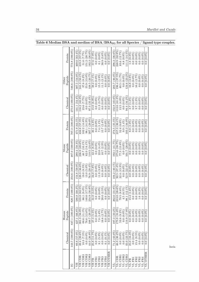
34 Marillet and Cazals
Table 6 Median BSA and median of BSA/BSAIG for all Species / ligand type couples.
Hum
anM
ouse
Oth
erC
hem
ical
Pep
tide
Pro
tein
Che
mic
alPep
tide
Pro
tein
Che
mic
alPep
tide
Pro
tein
IG14
3.7
(100
.0%
)64
7.1
(100
.0%
)82
0.7
(100
.0%
)25
4.6
(100
.0%
)48
7.0
(100
.0%
)70
7.3
(100
.0%
)27
5.0
(100
.0%
)54
6.6
(100
.0%
)77
3.8
(100
.0%
)
VH
89.8
(57.
0%)
427.
1(6
6.8%
)58
8.8
(68.
2%)
154.
8(5
9.9%
)28
9.4
(58.
3%)
471.
9(6
4.5%
)14
1.1
(54.
4%)
307.
5(5
4.0%
)46
9.0
(63.
4%)
VH
CD
R49
.4(3
9.6%
)38
1.3
(56.
9%)
518.
0(6
2.5%
)12
8.3
(46.
6%)
236.
9(4
9.6%
)43
4.8
(57.
5%)
116.
2(4
2.3%
)24
1.3
(50.
1%)
419.
3(5
7.5%
)V
HC
DR
110
.3(7
.5%
)68
.6(1
1.1%
)86
.1(9
.4%
)19
.0(8
.5%
)46
.7(1
0.1%
)10
2.2
(14.
8%)
23.6
(7.7
%)
37.6
(8.2
%)
51.6
(7.7
%)
VH
CD
R2
0.0
(0.0
%)
78.6
(12.
6%)
140.
6(1
7.5%
)13
.0(5
.0%
)62
.0(1
4.1%
)98
.1(1
4.3%
)0.
0(0
.0%
)55
.9(1
3.8%
)15
1.2
(20.
7%)
VH
CD
R3
44.0
(26.
9%)
188.
7(2
9.3%
)23
4.9
(30.
9%)
76.9
(29.
4%)
119.
5(2
4.0%
)20
7.7
(29.
0%)
97.3
(35.
4%)
108.
5(2
0.7%
)19
2.3
(26.
0%)
VH
FR
25.8
(11.
7%)
27.3
(5.5
%)
31.0
(3.5
%)
24.0
(7.8
%)
42.4
(8.3
%)
30.1
(4.3
%)
15.0
(6.9
%)
38.2
(7.1
%)
57.6
(7.9
%)
VH
FR
10.
0(0
.0%
)0.
0(0
.0%
)0.
0(0
.0%
)0.
0(0
.0%
)0.
0(0
.0%
)0.
0(0
.0%
)0.
0(0
.0%
)0.
0(0
.0%
)0.
0(0
.0%
)V
HFR
28.
1(5
.3%
)7.
8(1
.6%
)0.
0(0
.0%
)11
.9(3
.8%
)22
.0(4
.4%
)7.
4(1
.1%
)11
.3(3
.7%
)15
.5(2
.9%
)0.
1(0
.0%
)V
HFR
30.
0(0
.0%
)18
.6(2
.7%
)20
.0(2
.5%
)0.
0(0
.0%
)10
.7(2
.3%
)15
.7(2
.4%
)0.
0(0
.0%
)11
.5(2
.1%
)30
.9(3
.6%
)V
HFR
40.
1(0
.1%
)0.
0(0
.0%
)0.
0(0
.0%
)0.
0(0
.0%
)0.
0(0
.0%
)0.
0(0
.0%
)0.
0(0
.0%
)0.
0(0
.0%
)0.
0(0
.0%
)V
HO
TH
ER
0.0
(0.0
%)
0.0
(0.0
%)
0.0
(0.0
%)
0.0
(0.0
%)
0.0
(0.0
%)
0.0
(0.0
%)
0.0
(0.0
%)
0.0
(0.0
%)
0.0
(0.0
%)
VL
71.2
(43.
0%)
197.
3(3
3.2%
)26
2.6
(31.
8%)
104.
2(4
0.1%
)19
2.1
(41.
7%)
274.
5(3
5.5%
)13
2.8
(45.
6%)
203.
7(4
6.0%
)29
6.3
(36.
6%)
VL
CD
R46
.3(3
0.2%
)17
5.9
(31.
0%)
213.
0(2
6.6%
)92
.5(3
7.4%
)17
5.6
(38.
7%)
217.
3(3
0.1%
)11
3.6
(41.
3%)
196.
4(3
7.5%
)24
8.9
(32.
9%)
VL
CD
R1
0.0
(0.0
%)
53.8
(9.2
%)
79.5
(8.8
%)
32.4
(13.
3%)
77.5
(15.
9%)
52.4
(8.0
%)
13.5
(4.9
%)
49.5
(11.
7%)
83.6
(12.
7%)
VL
CD
R2
0.0
(0.0
%)
0.0
(0.0
%)
4.5
(0.5
%)
0.0
(0.0
%)
0.0
(0.0
%)
9.9
(1.4
%)
0.0
(0.0
%)
0.0
(0.0
%)
8.8
(0.9
%)
VL
CD
R3
45.0
(23.
7%)
114.
9(1
7.9%
)98
.1(1
2.1%
)52
.9(2
2.4%
)10
1.7
(20.
6%)
103.
3(1
6.0%
)94
.4(3
4.2%
)12
4.6
(23.
2%)
111.
4(1
4.5%
)V
LFR
25.0
(16.
3%)
0.0
(0.0
%)
15.2
(1.6
%)
0.0
(0.0
%)
0.0
(0.0
%)
8.0
(1.0
%)
3.7
(1.2
%)
16.8
(2.8
%)
1.8
(0.3
%)
VL
FR
10.
0(0
.0%
)0.
0(0
.0%
)0.
0(0
.0%
)0.
0(0
.0%
)0.
0(0
.0%
)0.
0(0
.0%
)0.
0(0
.0%
)0.
0(0
.0%
)0.
0(0
.0%
)V
LFR
215
.4(9
.5%
)0.
0(0
.0%
)0.
0(0
.0%
)0.
0(0
.0%
)0.
0(0
.0%
)0.
0(0
.0%
)3.
7(1
.2%
)16
.2(2
.7%
)0.
0(0
.0%
)V
LFR
30.
0(0
.0%
)0.
0(0
.0%
)1.
6(0
.2%
)0.
0(0
.0%
)0.
0(0
.0%
)0.
0(0
.0%
)0.
0(0
.0%
)0.
0(0
.0%
)0.
0(0
.0%
)V
LFR
40.
0(0
.0%
)0.
0(0
.0%
)0.
0(0
.0%
)0.
0(0
.0%
)0.
0(0
.0%
)0.
0(0
.0%
)0.
0(0
.0%
)0.
0(0
.0%
)0.
0(0
.0%
)V
LO
TH
ER
0.0
(0.0
%)
0.0
(0.0
%)
0.0
(0.0
%)
0.0
(0.0
%)
0.0
(0.0
%)
0.0
(0.0
%)
0.0
(0.0
%)
0.0
(0.0
%)
0.0
(0.0
%)
Inria

Dissecting Interfaces of Antibody - Antigen Complexes 35
Table 7 Confusion matrix for ligand type prediction. Results when the tree is run as aclassifier on the training data, for the pruned decision tree using variables bsaAg and bsaIG.
XXXXXXXXXXPredictedActual Chemical Peptide Protein
Chemical 75 3 1Peptide 2 104 16Protein 0 19 309
Figure 14 Rules characterizing the binding patch depending on the ligand types.See main text for details. The classification rules are: bsaAg ≥ 14.32: chemical ligand; 10.76 ≤bsaAg < 14.32: peptide ligand; bsaAg < 10.76 AND bsaIG < 5.697: peptide ligand; bsaAg < 10.76AND bsaIG ≥ 5.697: protein ligand.
Chemical Peptide Peptide Protein
bsaI G < 5.697
bsaA g >= 10.76
< 10.76
< 14.32 >= 5.697
bsaA g >= 14.32
RR n° 8770

36 Marillet and Cazals
Figure 15 Fraction of interface atoms contributed by the side-chains of the aminoacids for the VH and VL CDR. The central bar shows the median, the dot shows the average.
Other
(47)
Mou
se (3
37)
Human
(145
)
Chem
ical (7
7)
Prot
ein
(326
)
Pept
ide
(126
)
kapp
a (4
57)
lam
bda
(72)
0.4
0.5
0.6
0.7
0.8
0.9
1.0
1.1R
ela
tive n
um
ber
of
side c
hain
ato
ms
at
inte
rface
Inria

Dissecting Interfaces of Antibody - Antigen Complexes 37
6.2 Lengths of CDRWe now study the distribution of CDR lengths in our dataset. The IG - Ag complexes found inour dataset represent well the whole of existing subgroups, both for human and mice, in termsof [CDR1.CDR2] lengths (Supp. Tables 4 and 5).
Supp. Fig. 16 displays the abundance of combinations of CDR1/CDR2 and CDR3 lengthsfor VH and VL in the mouse and human. CDR1 and CDR2 are grouped in pairs because theyshare the same genomic origin whereas CDR3 is the product of an entirely different process [20,Chapter 6]. We now discuss in order: VH CDR and VL CDR of human IG, and VH CDR andVL CDR of murine IG.
Notice that when discussing the lengths of VH CDR, the human dataset consists of 140complexes instead of 145 because we discard 5 complexes whose VH CDR1 andVH CDR2 lengthsare aberrant (annotation not corresponding to any existing V-gene). For the same reason, weconsider 133 complexes for VL CDR in the human dataset after discarding 12 of them for aberrantVH CDR1 and VH CDR2 lengths.
For VH CDR in human, a striking 81% (113/140) of IG have both their VH CDR1 andVH CDR2 of length 8 although 6 different pairs occur. Except for a peak at 12 amino acids(15% of the dataset, 21/140), the lengths for 94% (132/140) of VH CDR3 are evenly distributedbetween 10 and 22 amino acids; even though it can reach a minimum of 6 and a maximum of 25amino acids.
For VL CDR in the human, 59% (79/133) of IG have their VL CDR1 and VL CDR2 of length6 an 3, respectively; for 22% (29/133) they are of length 8 and 3; and for 10% (14/133) theyare of length 7 and 3. Those three pairs therefore make up 92% of the human IG in this datasetalthough 6 distinct pairs actually occur. Interestingly, only VL CDR2 consisting of two aminoacids occur in the dataset. VL CDR3 is made of 9 amino acids in 56% (75/133) of the IG andof 10, 11 and 12 amino acids in 11% (15/133), 13% (18/133) and 7% (10/133) of the human IG.This makes 89% of all human IG in our dataset even though 9 distinct length actually occur.Interestingly, 35% (46/133) of the human IG have CDR of lengths 6, 3, and 9 for VL CDR1,VL CDR2 and VL CDR3, respectively. Moreover, the 5 combinations out of 26 ([6.3.9], [8.3.9],[6.3.10], [7.3.9], [6.3.11]) make 65% of the dataset.
From this analysis, it stems that:
• for human IG, the major locus of diversity is VH CDR3,
• whichever V gene is encoding the V-region, VL CDR2 is always of length 3,
• a single combination of VL CDR represents more than a third of the human dataset.
For VH CDR in mice, the situation is similar to that of human IG for VH CDR1 andVH CDR2: both are of length 8 for 66% (223/337) of the dataset although 5 distinct pairs occur.As for human IG, the most represented length for VH CDR3 is 12 (19% of the dataset, 65/337).Additionally, 71% (239/337) of murine VH CDR3 have between 11 and 15 amino acids while theminimum and maximum lengths are 5 and 20, respectively.
For VL CDR in the mouse, 38% (127/337) of IG have their VL CDR1 and VL CDR2 oflength 6 and 3, respectively. Additionally, they are of length 11 and 3 for 22% (73/337) of thedataset. A longer VL CDR1 is therefore more common in mice than in humans. Similarly tothe human dataset, only two IG have a VL CDR2 of length other than 3 (namely 7). Theoverwhelming majority (86%, 290/337) of murine IG have a VL CDR3 of length 9 althoughfour distinct lengths occur. Finally, two particular combinations of CDR are over-represented:[6.3.9] and [11.3.9] for [VL CDR1.VL CDR2.VL CDR3 ] which occur for 35% (119/337) and 19%(65/337) of the murine IG, respectively.
RR n° 8770

38 Marillet and Cazals
The two first points of the discussion for human IG also hold for murine IG. Moreover, twocombinations of VL CDR make up half of the dataset. Finally we notice that VL CDR1 is morevariable in length than VL CDR3.
Figure 16 Length of the CDR in number of amino acids. The four panels correspond tothe combinations {VH, VL } × {Human, Mouse}. For a given matrix, the gray shade encodesthe number of occurrences found in the dataset, from white (null count) to black (maximum forthat matrix, as indicated on the vertical bar on the right hand side.)
6 8 9 10 11 12 13 14 15 16 17 18 19 20 21 22 24 25Length in amino acids of CDR3
[10, 9]
[10, 7]
[9, 7]
[8, 10]
[8, 8]
[8, 7]
Length
s in
am
ino a
cids:
[C
DR
1,
CD
R2
]
Counts of the various combinations of CDR1/CDR2 against CDR3 for VH
0
2
4
6
8
10
12
14
16
18
Num
ber
of
occ
ure
nce
s
(a) VH, Human. Five complexes are discarded be-cause of aberrant VH CDR1 and VH CDR2 lengths.
5 6 7 8 9 10 11 12 13 14 15 16 17 18 19 20Length in amino acids of CDR3
[10, 7]
[9, 7]
[8, 10]
[8, 8]
[8, 7]
Length
s in
am
ino a
cids:
[C
DR
1,
CD
R2
]
Counts of the various combinations of CDR1/CDR2 against CDR3 for VH
0
5
10
15
20
25
30
35
40
44
Num
ber
of
occ
ure
nce
s
(b) VH, Mouse.
5 7 8 9 10 11 12 13 19Length in amino acids of CDR3
[12, 3]
[11, 3]
[9, 3]
[8, 3]
[7, 3]
[6, 3]
Length
s in
am
ino a
cids:
[C
DR
1,
CD
R2
]
Counts of the various combinations of CDR1/CDR2 against CDR3 for VL
0
5
10
15
20
25
30
35
40
4546
Num
ber
of
occ
ure
nce
s
(c) VL, Human. Twelve complexes are discarded be-cause of aberrant VL CDR1 and VL CDR2 lengths.The [CDR1.CDR2] lengths [6.3] characterize bothV-kappa and V-lambda. The other lengths char-acterize either V-kappa ([7.3], [11.3] and [12.3]) orV-lambda ([8.3] and [9.3]).
8 9 10 13Length in amino acids of CDR3
[12, 3]
[11, 3]
[10, 3]
[9, 3]
[7, 7]
[7, 3]
[6, 3]
[5, 3]
Length
s in
am
ino a
cids:
[C
DR
1,
CD
R2
]
Counts of the various combinations of CDR1/CDR2 against CDR3 for VL
0
12
24
36
48
60
72
84
96
108
119
Num
ber
of
occ
ure
nce
s
(d) VL, Mouse. The [CDR1.CDR2] lengths [7.7]and [9.3] characterize V-lambda. The other lengthscharacterize V-kappa.
Inria

Dissecting Interfaces of Antibody - Antigen Complexes 39
Figure 17 Buried Surface Area (A2): relative contributions of the CDR from VH
05
01
00
15
02
00
25
03
00
35
04
00
450
CD
R1
BSA
(2
)
0
50
10
0
15
0
20
0
25
0
30
0
35
0
40
0
CDR2 BSA (2
)V
H
05
01
00
15
02
00
25
030
035
040
04
50
CD
R1
BSA
(2
)
0
100
20
0
30
0
400
50
0
60
0
70
0
CDR3 BSA (2
)
VH
05
01
00
15
02
00
25
03
00
35
04
00
CD
R2
BSA
(2
)
0
10
0
20
0
30
0
40
0
50
0
60
0
70
0
CDR3 BSA (2
)
VH
CD
R1 B
SA
(2)
05
0 10
0 15
0 20
0 25
0 30
0 35
0 40
0 45
0CD
R2 B
SA (
2)
05010
015
020
025
030
035
0400
CDR3 BSA (2)
0100
20
03
00
40
05
00
60
07
00
VH
01
00
20
03
00
400
500
60
0
CD
R1
+ C
DR
2 B
SA
(2
)
0
100
20
0
30
0
400
50
0
60
0
70
0
CDR3 BSA (2
)
VH
Pepti
de
Pro
tein
Chem
ical
x =
y
RR n° 8770

40 Marillet and Cazals
Figure 18 Buried Surface Area (A2): relative contributions of the CDR from VL
05
01
00
15
02
00
25
03
00
350
400
CD
R1
BSA
(2
)
0
20
40
60
80
10
0
12
0
14
0
CDR2 BSA (2
)
VL
05
01
00
150
20
02
50
30
03
50
40
0
CD
R1
BSA
(2
)
0
50
10
0
15
0
200
250
30
0
CDR3 BSA (2
)
VL
02
04
06
08
01
00
12
01
40
CD
R2
BSA
(2
)
0
50
10
0
15
0
20
0
25
0
30
0
CDR3 BSA (2
)
VL
CD
R1 B
SA
(2)
05
0 10
0 15
0 20
0 25
0 30
0 35
0 40
0CD
R2 B
SA (
2)
02
0406
08010
012
014
0
CDR3 BSA (2)
050
10
0
15
0
200
25
0
300
VL
05
01
00
150
20
02
50
30
03
50
40
0
CD
R1
+ C
DR
2 B
SA
(2
)
0
50
10
0
15
0
200
250
30
0CDR3 BSA (
2)
VL
Pepti
de
Pro
tein
Chem
ical
x =
y
Inria

Dissecting Interfaces of Antibody - Antigen Complexes 41
6.3 Seams between CDR
In this section, we present seam statistics, for all ligands, and then for ligands of a given type.As opposed to Fig. 19, all figures were generated automatically. Thus, for the sake of uniformity,Fig. 9 reproduces the lengths displayed on Fig. 19.
Figure 19 Length of the seams between CDR for all atoms (whole dataset). Thecontacts between the 6 CDR are represented as a graph, with one edge between two CDRfor which seam statistics were collected. The statistic reported is the median value of all theobservations (in Å). The width of the edges is proportional to the median seam length.
15.9
7
5.94
14.55
24.6
26.8
9
10.0
30.89
VHCDR2
VHCDR3
VHCDR1
VLCDR2
VLCDR3
VLCDR1 Seam Median
lengthAveragelength
VH CDR1 - VH CDR2 24.6 24.4VH CDR1 - VH CDR3 30.9 31.8VH CDR1 - VL CDR3 0.0 0.8VH CDR2 - VH CDR3 0.0 5.3VH CDR2 - VL CDR1 0.0 0.0VH CDR2 - VL CDR3 0.0 1.3VH CDR3 - VL CDR1 10.0 10.1VH CDR3 - VL CDR2 5.9 6.4VH CDR3 - VL CDR3 14.5 15.2VL CDR1 - VL CDR2 16.0 16.2VL CDR1 - VL CDR3 26.9 26.1VL CDR2 - VL CDR3 0.0 0.7
Figure 20 Length of the seams between CDR for interface atoms (whole dataset).The contacts between the 6 CDR are represented as a graph, with one edge between two CDRfor which seam statistics were collected. The statistic reported is the median value of all theobservations (in Å). The width of the edges is proportional to the median seam length.
3.8
9
0.77
10.34
13.3
13.8
8
5.98
14.87
VHCDR2
VHCDR3
VHCDR1
VLCDR2
VLCDR3
VLCDR1
Seam Medianlength
Averagelength
VH CDR1 - VH CDR2 13.3 13.4VH CDR1 - VH CDR3 14.9 15.3VH CDR1 - VL CDR3 0.0 0.7VH CDR2 - VH CDR3 0.0 3.9VH CDR2 - VL CDR3 0.0 1.0VH CDR3 - VL CDR1 6.0 6.4VH CDR3 - VL CDR2 0.8 3.0VH CDR3 - VL CDR3 10.3 10.4VL CDR1 - VL CDR2 3.9 5.3VL CDR1 - VL CDR3 13.9 12.7VL CDR2 - VL CDR3 0.0 0.5
RR n° 8770

42 Marillet and Cazals
Figure 21 Length of the seams between CDR for protein ligands, all atoms. Thecontacts between the 6 CDR are represented as a graph, with one edge between two CDRfor which seam statistics were collected. The statistic reported is the median value of all theobservations (in Å). The width of the edges is proportional to the median seam length.
14.8
3
6.25
16.77
24.2
1
24.8
9
9.23
30.99
VHCDR2
VHCDR3
VHCDR1
VLCDR2
VLCDR3
VLCDR1
Seam Medianlength
Averagelength
VH CDR1 - VH CDR2 24.2 24.1VH CDR1 - VH CDR3 31.0 31.9VH CDR1 - VL CDR3 0.0 0.5VH CDR2 - VH CDR3 0.0 6.1VH CDR2 - VL CDR3 0.0 1.3VH CDR3 - VL CDR1 9.2 9.3VH CDR3 - VL CDR2 6.3 6.5VH CDR3 - VL CDR3 16.8 16.9VL CDR1 - VL CDR2 14.8 15.3VL CDR1 - VL CDR3 24.9 24.9VL CDR2 - VL CDR3 0.0 0.9
Figure 22 Length of the seams between CDR for protein ligands, interface atoms.The contacts between the 6 CDR are represented as a graph, with one edge between two CDRfor which seam statistics were collected. The statistic reported is the median value of all theobservations (in Å). The width of the edges is proportional to the median seam length.
5.6
7
2.29
10.95
14.9
2
13.9
7
5.52
16.05
VHCDR2
VHCDR3
VHCDR1
VLCDR2
VLCDR3
VLCDR1
Seam Medianlength
Averagelength
VH CDR1 - VH CDR2 14.9 15.2VH CDR1 - VH CDR3 16.1 16.9VH CDR1 - VL CDR3 0.0 0.5VH CDR2 - VH CDR3 0.0 4.5VH CDR2 - VL CDR3 0.0 1.0VH CDR3 - VL CDR1 5.5 5.8VH CDR3 - VL CDR2 2.3 3.8VH CDR3 - VL CDR3 10.9 10.9VL CDR1 - VL CDR2 5.7 6.3VL CDR1 - VL CDR3 14.0 13.0VL CDR2 - VL CDR3 0.0 0.6
Inria

Dissecting Interfaces of Antibody - Antigen Complexes 43
Figure 23 Length of the seams between CDR for peptide ligands, all atoms. Thecontacts between the 6 CDR are represented as a graph, with one edge between two CDRfor which seam statistics were collected. The statistic reported is the median value of all theobservations. The width of the edges is proportional to the median seam length (in Å).
18.3
55.81
11.78
24.5
9
28.7
2
10.63
27.84
VHCDR2
VHCDR3
VHCDR1
VLCDR2
VLCDR3
VLCDR1
Seam Medianlength
Averagelength
VH CDR1 - VH CDR2 24.6 24.4VH CDR1 - VH CDR3 27.8 30.3VH CDR1 - VL CDR3 0.0 0.8VH CDR2 - VH CDR3 0.0 3.6VH CDR2 - VL CDR3 0.0 1.0VH CDR3 - VL CDR1 10.6 11.0VH CDR3 - VL CDR2 5.8 6.4VH CDR3 - VL CDR3 11.8 12.7VL CDR1 - VL CDR2 18.3 17.8VL CDR1 - VL CDR3 28.7 28.1VL CDR2 - VL CDR3 0.0 0.4
Figure 24 Length of the seams between CDR for peptide ligands, interface atoms.The contacts between the 6 CDR are represented as a graph, with one edge between two CDRfor which seam statistics were collected. The statistic reported is the median value of all theobservations (in Å). The width of the edges is proportional to the median seam length.
3.2
6
0.14
9.7
11.8
6
14.7
2
8.2
15.05
VHCDR2
VHCDR3
VHCDR1
VLCDR2
VLCDR3
VLCDR1
Seam Medianlength
Averagelength
VH CDR1 - VH CDR2 11.9 12.7VH CDR1 - VH CDR3 15.0 14.3VH CDR1 - VL CDR3 0.0 0.8VH CDR2 - VH CDR3 0.0 3.0VH CDR2 - VL CDR3 0.0 0.7VH CDR3 - VL CDR1 8.2 7.9VH CDR3 - VL CDR2 0.1 2.3VH CDR3 - VL CDR3 9.7 9.9VL CDR1 - VL CDR2 3.3 4.8VL CDR1 - VL CDR3 14.7 14.5VL CDR2 - VL CDR3 0.0 0.3
RR n° 8770

44 Marillet and Cazals
Figure 25 Length of the seams between CDR for chemical ligands, all atoms. Thecontacts between the 6 CDR are represented as a graph, with one edge between two CDRfor which seam statistics were collected. The statistic reported is the median value of all theobservations (in Å). The width of the edges is proportional to the median seam length.
17.8
1
5.22
11.89
26.1
1
28.0
5
12.7633.1
VHCDR2
VHCDR3
VHCDR1
VLCDR2
VLCDR3
VLCDR1 Seam Median
lengthAveragelength
VH CDR1 - VH CDR2 26.1 25.8VH CDR1 - VH CDR3 33.1 33.8VH CDR1 - VL CDR3 0.0 2.0VH CDR2 - VH CDR3 0.0 5.0VH CDR2 - VL CDR1 0.0 0.1VH CDR2 - VL CDR3 0.0 1.7VH CDR3 - VL CDR1 12.8 12.2VH CDR3 - VL CDR2 5.2 6.1VH CDR3 - VL CDR3 11.9 12.1VL CDR1 - VL CDR2 17.8 17.1VL CDR1 - VL CDR3 28.1 28.3VL CDR2 - VL CDR3 0.0 0.4
Figure 26 Length of the seams between CDR for chemical ligands, interface atoms.The contacts between the 6 CDR are represented as a graph, with one edge between two CDRfor which seam statistics were collected. The statistic reported is the median value of all theobservations (in Å). The width of the edges is proportional to the median seam length.
8.94
6.5
3
9.84 8.676.53
VHCDR2
VHCDR3
VHCDR1
VLCDR2
VLCDR3
VLCDR1
Seam Medianlength
Averagelength
VH CDR1 - VH CDR2 6.5 7.1VH CDR1 - VH CDR3 9.8 10.3VH CDR1 - VL CDR3 0.0 1.8VH CDR2 - VH CDR3 0.0 2.6VH CDR2 - VL CDR3 0.0 1.3VH CDR3 - VL CDR1 6.5 6.6VH CDR3 - VL CDR2 0.0 1.0VH CDR3 - VL CDR3 8.9 9.5VL CDR1 - VL CDR2 0.0 1.5VL CDR1 - VL CDR3 8.7 9.0VL CDR2 - VL CDR3 0.0 0.3
Inria

Dissecting Interfaces of Antibody - Antigen Complexes 45
Figure 27 Length of the seams between CDR for VL = V-kappa, all atoms. Thecontacts between the 6 CDR are represented as a graph, with one edge between two CDRfor which seam statistics were collected. The statistic reported is the median value of all theobservations (in Å). The width of the edges is proportional to the median seam length.
16.2
86.1
14.89
24.7
26.5
9.44
31.0
VHCDR2
VHCDR3
VHCDR1
VLCDR2
VLCDR3
VLCDR1 Seam Median
lengthAveragelength
VH CDR1 - VH CDR2 24.7 24.7VH CDR1 - VH CDR3 31.0 31.8VH CDR1 - VL CDR3 0.0 0.8VH CDR2 - VH CDR3 0.0 5.1VH CDR2 - VL CDR1 0.0 0.0VH CDR2 - VL CDR3 0.0 1.2VH CDR3 - VL CDR1 9.4 9.6VH CDR3 - VL CDR2 6.1 6.4VH CDR3 - VL CDR3 14.9 15.3VL CDR1 - VL CDR2 16.3 16.4VL CDR1 - VL CDR3 26.5 25.8VL CDR2 - VL CDR3 0.0 0.8
Figure 28 Length of the seams between CDR for VL = V-kappa, interface atoms.The contacts between the 6 CDR are represented as a graph, with one edge between two CDRfor which seam statistics were collected. The statistic reported is the median value of all theobservations (in Å). The width of the edges is proportional to the median seam length.
3.5
9
0.7
10.4
13.3
14.1
8
5.64
14.85
VHCDR2
VHCDR3
VHCDR1
VLCDR2
VLCDR3
VLCDR1
Seam Medianlength
Averagelength
VH CDR1 - VH CDR2 13.3 13.5VH CDR1 - VH CDR3 14.8 15.1VH CDR1 - VL CDR3 0.0 0.7VH CDR2 - VH CDR3 0.0 3.8VH CDR2 - VL CDR3 0.0 0.9VH CDR3 - VL CDR1 5.6 6.2VH CDR3 - VL CDR2 0.7 3.0VH CDR3 - VL CDR3 10.4 10.7VL CDR1 - VL CDR2 3.6 5.0VL CDR1 - VL CDR3 14.2 13.0VL CDR2 - VL CDR3 0.0 0.6
RR n° 8770

46 Marillet and Cazals
Figure 29 Length of the seams between CDR for VL = V-lambda, all atoms. Thecontacts between the 6 CDR are represented as a graph, with one edge between two CDRfor which seam statistics were collected. The statistic reported is the median value of all theobservations (in Å). The width of the edges is proportional to the median seam length.
14.0
5
3.78
12.55
20.4
28.2
3
12.16
3.23
29.94
VHCDR2
VHCDR3
VHCDR1
VLCDR2
VLCDR3
VLCDR1
Seam Medianlength
Averagelength
VH CDR1 - VH CDR2 20.4 22.9VH CDR1 - VH CDR3 29.9 31.8VH CDR1 - VL CDR3 0.0 1.0VH CDR2 - VH CDR3 3.2 6.5VH CDR2 - VL CDR3 0.0 1.8VH CDR3 - VL CDR1 12.2 13.0VH CDR3 - VL CDR2 3.8 6.6VH CDR3 - VL CDR3 12.6 14.5VL CDR1 - VL CDR2 14.0 14.9VL CDR1 - VL CDR3 28.2 28.4
Figure 30 Length of the seams between CDR for VL = V-lambda, interface atoms.The contacts between the 6 CDR are represented as a graph, with one edge between two CDRfor which seam statistics were collected. The statistic reported is the median value of all theobservations (in Å). The width of the edges is proportional to the median seam length.
5.2
5
0.86
8.95
13.4
2
10.9
9
8.44
15.25
VHCDR2
VHCDR3
VHCDR1
VLCDR2
VLCDR3
VLCDR1
Seam Medianlength
Averagelength
VH CDR1 - VH CDR2 13.4 13.2VH CDR1 - VH CDR3 15.3 16.3VH CDR1 - VL CDR3 0.0 0.9VH CDR2 - VH CDR3 0.0 4.3VH CDR2 - VL CDR3 0.0 1.1VH CDR3 - VL CDR1 8.4 8.0VH CDR3 - VL CDR2 0.9 3.2VH CDR3 - VL CDR3 9.0 9.0VL CDR1 - VL CDR2 5.3 6.8VL CDR1 - VL CDR3 11.0 10.9
Inria

Dissecting Interfaces of Antibody - Antigen Complexes 47
Figure 31 Predicted versus experimental affinities for IG - Ag complexes. Dashed,dash-dotted and dotted lines respectively show errors of±1.4, ±2.8, ±4.2 kcal/mol, correspondingto Kd approximated within one, two and three orders of magnitude.
●
●
●
●
●
●
● ●
●
●
●
●
●
●
8 9 10 11 12 13
11.0
11.5
12.0
12.5
Experimental affinity (kcal/mol)
Pre
dict
ed a
ffini
ty (k
cal/m
ol)
Figure 32 Distribution of the length of the seams between CDR. Comparison betweenVL V-kappa and V-lambda, atoms at interface.
VH CDR1
- VH C
DR2
VH CDR1
- VH C
DR3
VH CDR1
- VL CDR1
VH CDR1
- VL CDR2
VH CDR1
- VL CDR3
VH CDR2
- VH C
DR3
VH CDR2
- VL CDR1
VH CDR2
- VL CDR2
VH CDR2
- VL CDR3
VH CDR3
- VL CDR1
VH CDR3
- VL CDR2
VH CDR3
- VL CDR3
VL CDR1
- VL CDR2
VL CDR1
- VL CDR3
VL CDR2
- VL CDR3
10
0
10
20
30
40
50
Sum
of
length
of
edges
at
fronti
er
kappa (457 structures)
VH CDR1
- VH C
DR2
VH CDR1
- VH C
DR3
VH CDR1
- VL CDR1
VH CDR1
- VL CDR2
VH CDR1
- VL CDR3
VH CDR2
- VH C
DR3
VH CDR2
- VL CDR1
VH CDR2
- VL CDR2
VH CDR2
- VL CDR3
VH CDR3
- VL CDR1
VH CDR3
- VL CDR2
VH CDR3
- VL CDR3
VL CDR1
- VL CDR2
VL CDR1
- VL CDR3
VL CDR2
- VL CDR3
5
0
5
10
15
20
25
30
35
40
Sum
of
length
of
edges
at
fronti
er
lambda (72 structures)
RR n° 8770

48 Marillet and Cazals
Figure 33 Distribution of the length of the seams between CDR. Comparison betweenligand types, atoms at interface.
VH CDR1
- VH C
DR2
VH CDR1
- VH C
DR3
VH CDR1
- VL CDR1
VH CDR1
- VL CDR2
VH CDR1
- VL CDR3
VH CDR2
- VH C
DR3
VH CDR2
- VL CDR1
VH CDR2
- VL CDR2
VH CDR2
- VL CDR3
VH CDR3
- VL CDR1
VH CDR3
- VL CDR2
VH CDR3
- VL CDR3
VL CDR1
- VL CDR2
VL CDR1
- VL CDR3
VL CDR2
- VL CDR3
5
0
5
10
15
20
25
30
Sum
of
length
of
edges
at
fronti
er Chemical (77 structures)
VH CDR1
- VH C
DR2
VH CDR1
- VH C
DR3
VH CDR1
- VL CDR1
VH CDR1
- VL CDR2
VH CDR1
- VL CDR3
VH CDR2
- VH C
DR3
VH CDR2
- VL CDR1
VH CDR2
- VL CDR2
VH CDR2
- VL CDR3
VH CDR3
- VL CDR1
VH CDR3
- VL CDR2
VH CDR3
- VL CDR3
VL CDR1
- VL CDR2
VL CDR1
- VL CDR3
VL CDR2
- VL CDR3
10
0
10
20
30
40
50
Sum
of
length
of
edges
at
fronti
er Protein (326 structures)
VH CDR1
- VH C
DR2
VH CDR1
- VH C
DR3
VH CDR1
- VL CDR1
VH CDR1
- VL CDR2
VH CDR1
- VL CDR3
VH CDR2
- VH C
DR3
VH CDR2
- VL CDR1
VH CDR2
- VL CDR2
VH CDR2
- VL CDR3
VH CDR3
- VL CDR1
VH CDR3
- VL CDR2
VH CDR3
- VL CDR3
VL CDR1
- VL CDR2
VL CDR1
- VL CDR3
VL CDR2
- VL CDR3
5
0
5
10
15
20
25
30
35
40
Sum
of
length
of
edges
at
fronti
er Peptide (126 structures)
Inria

Dissecting Interfaces of Antibody - Antigen Complexes 49
Figure 34 Distribution of the length of the seams between CDR. Comparison betweenspecies, atoms at interface.
VH CDR1
- VH C
DR2
VH CDR1
- VH C
DR3
VH CDR1
- VL CDR1
VH CDR1
- VL CDR2
VH CDR1
- VL CDR3
VH CDR2
- VH C
DR3
VH CDR2
- VL CDR1
VH CDR2
- VL CDR2
VH CDR2
- VL CDR3
VH CDR3
- VL CDR1
VH CDR3
- VL CDR2
VH CDR3
- VL CDR3
VL CDR1
- VL CDR2
VL CDR1
- VL CDR3
VL CDR2
- VL CDR3
5
0
5
10
15
20
25
30
35
Sum
of
length
of
edges
at
fronti
er Other (47 structures)
VH CDR1
- VH C
DR2
VH CDR1
- VH C
DR3
VH CDR1
- VL CDR1
VH CDR1
- VL CDR2
VH CDR1
- VL CDR3
VH CDR2
- VH C
DR3
VH CDR2
- VL CDR1
VH CDR2
- VL CDR2
VH CDR2
- VL CDR3
VH CDR3
- VL CDR1
VH CDR3
- VL CDR2
VH CDR3
- VL CDR3
VL CDR1
- VL CDR2
VL CDR1
- VL CDR3
VL CDR2
- VL CDR3
10
0
10
20
30
40
50
Sum
of
length
of
edges
at
fronti
er Mouse (337 structures)
VH CDR1
- VH C
DR2
VH CDR1
- VH C
DR3
VH CDR1
- VL CDR1
VH CDR1
- VL CDR2
VH CDR1
- VL CDR3
VH CDR2
- VH C
DR3
VH CDR2
- VL CDR1
VH CDR2
- VL CDR2
VH CDR2
- VL CDR3
VH CDR3
- VL CDR1
VH CDR3
- VL CDR2
VH CDR3
- VL CDR3
VL CDR1
- VL CDR2
VL CDR1
- VL CDR3
VL CDR2
- VL CDR3
10
0
10
20
30
40
50
Sum
of
length
of
edges
at
fronti
er Human (145 structures)
Figure 35 Distribution of the length of the seams between CDR. Comparison betweenVL V-lambda and V-kappa, all atoms.
VH CDR1
- VH C
DR2
VH CDR1
- VH C
DR3
VH CDR1
- VL CDR1
VH CDR1
- VL CDR2
VH CDR1
- VL CDR3
VH CDR2
- VH C
DR3
VH CDR2
- VL CDR1
VH CDR2
- VL CDR2
VH CDR2
- VL CDR3
VH CDR3
- VL CDR1
VH CDR3
- VL CDR2
VH CDR3
- VL CDR3
VL CDR1
- VL CDR2
VL CDR1
- VL CDR3
VL CDR2
- VL CDR3
10
0
10
20
30
40
50
60
70
80
Sum
of
length
of
edges
at
fronti
er
kappa (457 structures)
VH CDR1
- VH C
DR2
VH CDR1
- VH C
DR3
VH CDR1
- VL CDR1
VH CDR1
- VL CDR2
VH CDR1
- VL CDR3
VH CDR2
- VH C
DR3
VH CDR2
- VL CDR1
VH CDR2
- VL CDR2
VH CDR2
- VL CDR3
VH CDR3
- VL CDR1
VH CDR3
- VL CDR2
VH CDR3
- VL CDR3
VL CDR1
- VL CDR2
VL CDR1
- VL CDR3
VL CDR2
- VL CDR3
10
0
10
20
30
40
50
60
Sum
of
length
of
edges
at
fronti
er
lambda (72 structures)
RR n° 8770

50 Marillet and Cazals
Figure 36 Distribution of the length of the seams between CDR. Comparison betweenligand types, all atoms.
VH CDR1
- VH C
DR2
VH CDR1
- VH C
DR3
VH CDR1
- VL CDR1
VH CDR1
- VL CDR2
VH CDR1
- VL CDR3
VH CDR2
- VH C
DR3
VH CDR2
- VL CDR1
VH CDR2
- VL CDR2
VH CDR2
- VL CDR3
VH CDR3
- VL CDR1
VH CDR3
- VL CDR2
VH CDR3
- VL CDR3
VL CDR1
- VL CDR2
VL CDR1
- VL CDR3
VL CDR2
- VL CDR3
10
0
10
20
30
40
50
60
Sum
of
length
of
edges
at
fronti
er Chemical (77 structures)
VH CDR1
- VH C
DR2
VH CDR1
- VH C
DR3
VH CDR1
- VL CDR1
VH CDR1
- VL CDR2
VH CDR1
- VL CDR3
VH CDR2
- VH C
DR3
VH CDR2
- VL CDR1
VH CDR2
- VL CDR2
VH CDR2
- VL CDR3
VH CDR3
- VL CDR1
VH CDR3
- VL CDR2
VH CDR3
- VL CDR3
VL CDR1
- VL CDR2
VL CDR1
- VL CDR3
VL CDR2
- VL CDR3
10
0
10
20
30
40
50
60
70
80
Sum
of
length
of
edges
at
fronti
er Protein (326 structures)
VH CDR1
- VH C
DR2
VH CDR1
- VH C
DR3
VH CDR1
- VL CDR1
VH CDR1
- VL CDR2
VH CDR1
- VL CDR3
VH CDR2
- VH C
DR3
VH CDR2
- VL CDR1
VH CDR2
- VL CDR2
VH CDR2
- VL CDR3
VH CDR3
- VL CDR1
VH CDR3
- VL CDR2
VH CDR3
- VL CDR3
VL CDR1
- VL CDR2
VL CDR1
- VL CDR3
VL CDR2
- VL CDR3
10
0
10
20
30
40
50
60
70
Sum
of
length
of
edges
at
fronti
er Peptide (126 structures)
Inria

Dissecting Interfaces of Antibody - Antigen Complexes 51
Figure 37 Distribution of the length of the seams between CDR. Comparison betweenspecies, all atoms.
VH CDR1
- VH C
DR2
VH CDR1
- VH C
DR3
VH CDR1
- VL CDR1
VH CDR1
- VL CDR2
VH CDR1
- VL CDR3
VH CDR2
- VH C
DR3
VH CDR2
- VL CDR1
VH CDR2
- VL CDR2
VH CDR2
- VL CDR3
VH CDR3
- VL CDR1
VH CDR3
- VL CDR2
VH CDR3
- VL CDR3
VL CDR1
- VL CDR2
VL CDR1
- VL CDR3
VL CDR2
- VL CDR3
10
0
10
20
30
40
50
60
Sum
of
length
of
edges
at
fronti
er Other (47 structures)
VH CDR1
- VH C
DR2
VH CDR1
- VH C
DR3
VH CDR1
- VL CDR1
VH CDR1
- VL CDR2
VH CDR1
- VL CDR3
VH CDR2
- VH C
DR3
VH CDR2
- VL CDR1
VH CDR2
- VL CDR2
VH CDR2
- VL CDR3
VH CDR3
- VL CDR1
VH CDR3
- VL CDR2
VH CDR3
- VL CDR3
VL CDR1
- VL CDR2
VL CDR1
- VL CDR3
VL CDR2
- VL CDR3
10
0
10
20
30
40
50
60
Sum
of
length
of
edges
at
fronti
er Mouse (337 structures)
VH CDR1
- VH C
DR2
VH CDR1
- VH C
DR3
VH CDR1
- VL CDR1
VH CDR1
- VL CDR2
VH CDR1
- VL CDR3
VH CDR2
- VH C
DR3
VH CDR2
- VL CDR1
VH CDR2
- VL CDR2
VH CDR2
- VL CDR3
VH CDR3
- VL CDR1
VH CDR3
- VL CDR2
VH CDR3
- VL CDR3
VL CDR1
- VL CDR2
VL CDR1
- VL CDR3
VL CDR2
- VL CDR3
10
0
10
20
30
40
50
60
70
80
Sum
of
length
of
edges
at
fronti
er Human (145 structures)
Correlation between seam length and interface curvature / ligand size. We investi-gated the correlation between individual seams lengths and three parameters: the size of the Agand the curvature of the interface on both the IG and Ag side (Supp. Tables 8-13).
Note that the values in Supp. Tables 8 are the opposite of those in Supp. Tables 10. Thesame applies for Supp. Tables 9 and 11. This is expected since the curvatures of both size of theinterface are complementary. We therefore limit our discussion to Supp. Tables 8, 9, 12 and 13.
Overall, the correlation are low, ranging from -0.37 to 0.21 for linear relationships and from-0.36 to 0.31 for non-linear monotonous relationships.
Considering the seams between all atoms, linear correlations range between -0.37 (VH CDR3-VL CDR3 versus interface curvature) and 0.21 (VH CDR3- VL CDR3 versus Ag size) andnon-linear monotonous correlations range between -0.36 (VH CDR3- VL CDR3 versus interfacecurvature) and 0.31 (VH CDR3- VL CDR3 versus interface Ag size).
Considering the seams between interface atoms, linear correlations range between -0.22 (VH CDR1-VH CDR3 versus interface curvature) and 0.19 (VH CDR1- VL CDR3 vs interface curvature andVH CDR1- VH CDR3 versus Ag size), and non-linear monotonous correlations range between-0.23 (VH CDR1- VL CDR3 vs Ag size) and 0.29 (VH CDR1- VH CDR3 versus interface Agsize).
RR n° 8770

52 Marillet and Cazals
Table 8 Correlation between length of seams at interface and curvature of the in-terface, IG side
VH CDR2 VH CDR3 VL CDR1 VL CDR2 VL CDR3
VH CDR1
Pearson -0.11 -0.22 - - 0.19p-value 8.236e-03 4.548e-07 - - 8.130e-06Spearman -0.12 -0.20 - - 0.18p-value 7.876e-03 2.777e-06 - - 3.107e-05
VH CDR2
Pearson - -0.20 - - -0.05p-value - 5.416e-06 - - 2.711e-01Spearman - -0.22 - - -0.04p-value - 3.852e-07 - - 3.135e-01
VH CDR3
Pearson - - 0.01 -0.15 0.06p-value - - 7.612e-01 5.687e-04 1.876e-01Spearman - - -0.02 -0.17 0.02p-value - - 7.017e-01 1.060e-04 5.906e-01
VL CDR1
Pearson - - - -0.17 0.07p-value - - - 1.108e-04 1.259e-01Spearman - - - -0.18 0.07p-value - - - 2.516e-05 1.264e-01
VL CDR2
Pearson - - - - -0.02p-value - - - - 6.953e-01Spearman - - - - -0.01p-value - - - - 8.840e-01
Table 9 Correlation between length of seams and curvature of the interface, IG sideVH CDR2 VH CDR3 VL CDR1 VL CDR2 VL CDR3
VH CDR1
Pearson 0.16 -0.08 - - 0.18p-value 1.679e-04 7.329e-02 - - 4.345e-05Spearman 0.15 -0.04 - - 0.14p-value 5.268e-04 3.527e-01 - - 1.399e-03
VH CDR2
Pearson - -0.22 0.03 - -0.07p-value - 3.833e-07 4.445e-01 - 9.498e-02Spearman - -0.23 0.04 - -0.07p-value - 1.160e-07 3.843e-01 - 1.171e-01
VH CDR3
Pearson - - -0.00 -0.05 -0.37p-value - - 9.254e-01 2.514e-01 3.028e-18Spearman - - -0.02 -0.07 -0.36p-value - - 7.084e-01 1.225e-01 2.819e-17
VL CDR1
Pearson - - - 0.17 0.17p-value - - - 5.701e-05 6.837e-05Spearman - - - 0.19 0.21p-value - - - 1.242e-05 7.123e-07
VL CDR2
Pearson - - - - -0.06p-value - - - - 1.439e-01Spearman - - - - -0.06p-value - - - - 2.063e-01
Inria

Dissecting Interfaces of Antibody - Antigen Complexes 53
Table 10 Correlation between length of seams at interface and curvature of theinterface, Ag side
VH CDR2 VH CDR3 VL CDR1 VL CDR2 VL CDR3
VH CDR1
Pearson 0.11 0.22 - - -0.19p-value 8.236e-03 4.548e-07 - - 8.130e-06Spearman 0.12 0.20 - - -0.18p-value 7.876e-03 2.777e-06 - - 3.107e-05
VH CDR2
Pearson - 0.20 - - 0.05p-value - 5.416e-06 - - 2.711e-01Spearman - 0.22 - - 0.04p-value - 3.852e-07 - - 3.135e-01
VH CDR3
Pearson - - -0.01 0.15 -0.06p-value - - 7.612e-01 5.687e-04 1.876e-01Spearman - - 0.02 0.17 -0.02p-value - - 7.017e-01 1.060e-04 5.906e-01
VL CDR1
Pearson - - - 0.17 -0.07p-value - - - 1.108e-04 1.259e-01Spearman - - - 0.18 -0.07p-value - - - 2.516e-05 1.264e-01
VL CDR2
Pearson - - - - 0.02p-value - - - - 6.953e-01Spearman - - - - 0.01p-value - - - - 8.840e-01
Table 11 Correlation between length of seams and curvature of the interface, Agside
VH CDR2 VH CDR3 VL CDR1 VL CDR2 VL CDR3
VH CDR1
Pearson -0.16 0.08 - - -0.18p-value 1.679e-04 7.329e-02 - - 4.345e-05Spearman -0.15 0.04 - - -0.14p-value 5.268e-04 3.527e-01 - - 1.399e-03
VH CDR2
Pearson - 0.22 -0.03 - 0.07p-value - 3.833e-07 4.445e-01 - 9.498e-02Spearman - 0.23 -0.04 - 0.07p-value - 1.160e-07 3.843e-01 - 1.171e-01
VH CDR3
Pearson - - 0.00 0.05 0.37p-value - - 9.254e-01 2.514e-01 3.028e-18Spearman - - 0.02 0.07 0.36p-value - - 7.084e-01 1.225e-01 2.819e-17
VL CDR1
Pearson - - - -0.17 -0.17p-value - - - 5.701e-05 6.837e-05Spearman - - - -0.19 -0.21p-value - - - 1.242e-05 7.123e-07
VL CDR2
Pearson - - - - 0.06p-value - - - - 1.439e-01Spearman - - - - 0.06p-value - - - - 2.063e-01
RR n° 8770

54 Marillet and Cazals
Table 12 Correlation between length of seams at interface and Ag sizeVH CDR2 VH CDR3 VL CDR1 VL CDR2 VL CDR3
VH CDR1
Pearson 0.06 0.19 - - -0.15p-value 1.730e-01 1.285e-05 - - 4.892e-04Spearman 0.23 0.29 - - -0.23p-value 7.413e-08 1.448e-11 - - 9.712e-08
VH CDR2
Pearson - 0.11 - - 0.00p-value - 1.447e-02 - - 9.462e-01Spearman - 0.13 - - -0.04p-value - 2.323e-03 - - 4.214e-01
VH CDR3
Pearson - - -0.00 0.04 0.08p-value - - 9.493e-01 3.680e-01 5.721e-02Spearman - - -0.03 0.21 0.13p-value - - 5.235e-01 9.478e-07 2.135e-03
VL CDR1
Pearson - - - 0.13 -0.17p-value - - - 2.646e-03 8.668e-05Spearman - - - 0.22 -0.05p-value - - - 5.204e-07 2.238e-01
VL CDR2
Pearson - - - - 0.01p-value - - - - 7.755e-01Spearman - - - - 0.09p-value - - - - 3.920e-02
Table 13 Correlation between length of seams and Ag sizeVH CDR2 VH CDR3 VL CDR1 VL CDR2 VL CDR3
VH CDR1
Pearson -0.11 0.14 - - -0.13p-value 1.532e-02 1.373e-03 - - 1.910e-03Spearman -0.12 0.06 - - -0.19p-value 6.057e-03 1.838e-01 - - 1.204e-05
VH CDR2
Pearson - 0.11 -0.03 - -0.00p-value - 1.554e-02 4.884e-01 - 9.146e-01Spearman - 0.08 -0.07 - -0.03p-value - 5.079e-02 1.192e-01 - 5.038e-01
VH CDR3
Pearson - - 0.09 -0.08 0.21p-value - - 4.017e-02 7.548e-02 6.631e-07Spearman - - -0.02 0.00 0.31p-value - - 7.262e-01 9.625e-01 1.407e-13
VL CDR1
Pearson - - - -0.18 -0.26p-value - - - 2.731e-05 2.120e-09Spearman - - - -0.24 -0.29p-value - - - 2.542e-08 7.610e-12
VL CDR2
Pearson - - - - 0.01p-value - - - - 8.804e-01Spearman - - - - 0.11p-value - - - - 1.410e-02
Inria

Dissecting Interfaces of Antibody - Antigen Complexes 55
These values are too low to bring about any meaningful conclusions, but we notice that 1) theprevious highest correlations only involve VH CDR3- VL CDR3 or seams between VH CDR1 andthe CDR3 from both VH and VL; 2) the seams VH CDR3- VL CDR3 and VH CDR1- VH CDR3show the highest absolute linear correlations with both interface curvature and Ag size for allatoms and interface atoms respectively.
RR n° 8770

56 Marillet and Cazals
7 Supplemental: Dataset Curation
7.1 Inferring Canonical Complexes
A canonical configuration for a IMGT/3Dstructure-DB IMGT-PDB file is as follows: one Hchain, one L chain, one ligand. A non canonical configuration may occur for different reasons:
• The asymmetric unit of the crystal structure contains two or more Fabs.
• Several molecules have co-cristallized with the IG - Ag complex.
• Two IG chains, H and L, and one Ag chain are found but the IG chains are not annotatedas forming a receptor in the IMGT 410 section.
• An IG receptor is annotated as containing more than two chains.
• The ligand is a multi-chain protein
The following issues are faced:
• A file may not be canonical i.e. there might be several complexes in a single file.
• There might be some issues with the numbering of the chains.
• There might be missing data (residues, chains information, labels)
• Several complexes might be similar and bias the results.
• Some molecules annotated as ligand may actually be buffer molecules (e.g. glycerol)
• Some purification proteins remain (e.g. protein L, A or G) and do not engage in specificcontacts with the IG
Using the Voronoi interface model presented in section 2.1, we proceed in two steps. First,we infer the chains pairings in every file which does not contain a canonical complex. For this,we compute the interfaces between all pairs of chains. We then group L and H chains in pairs forwhich the number of atoms at the interface is the highest. We then assign the ligand(s) chainsto the HL pairs if they make contacts with either chain.
Note that in the case where an Ag is in contact with several IG, it will be assigned to bothIG.
Finally, all buffer molecules and IG purification proteins (namely protein L, A and G whoseannotated name satisfy the regexp "immunoglobulin g-binding|protein[ ]+[gl]($|\s|\’)|glycerol"are removed from the files because they are not representative of IG - Ag interactions.
Inria

Dissecting Interfaces of Antibody - Antigen Complexes 57
Figure 38 Inferring complexes within an IMGT-PDB file (IMGT-1GGI.pdb): crystalstructure in its van der Waals representation, and associated connectivity graphfrom which two complexes are defined. (Left) The seven chains from the file: L (blue), H(red), P (grey), J (yellow), M (orange), Q (chartreuse green). (Right) The graph summarizesthe connectivity between chains computed by intervor-bif, from the package Intervor. Verticesare chains (with their IDs) and the edges are weighted by the number of atoms at the interface.Here H and J are the Fab heavy chains, L and M are the Fab light chains and P and Q are theligand chains. Thus, this file defines two complexes.
H
L
394
P
92
J
78
M
409
Q
91
68 7 60
Crystal contacts. The previous automatic detection raises the problem of crystal contacts,since complexes reported might be false positives.
They could potentially be ruled out by using a cutoff such as the minimal number of atomsat an interface to be considered significant, however, there might also be few contacts betweena Fab and a small ligand. It is therefore necessary to study the distribution of the number ofatoms at the interface for different classes of ligands to set a specific cutoff.
To circumvent this issue, we currently exclude from the analysis complexes which do not haveat least one contact with the variable domain (CDR or FR).
7.2 Removing redundanciesRedundant complexes may come from two sources: the same complex may be found in the sameasymmetric crystal unit, or it may be found in two different IMGT-PDB files.
We therefore need to remove the redundancy of the dataset to avoid biasing the statistics.For this, we need to consider similarities at the interface level. Once all complexes are extractedfrom the database, we need to compare the interfaces of all pairs of complexes, group complexeshaving a similar interface, and keep one representative complex for each group.
Currently, we rely on a quick method based upon IMGT labels. We consider triplets formedby the IMGT labels of both IG chains and the Ag chain. We record triplets which have alreadybeen included in the analysis and exclude complexes which make the same triplet.
RR n° 8770

58 Marillet and Cazals
Contents1 Introduction 3
1.1 Immunoglobulins and the immune response . . . . . . . . . . . . . . . . . . . . . 31.2 IG - Ag complexes under the structural lens . . . . . . . . . . . . . . . . . . . . . 3
2 Material and Methods 52.1 Voronoi Interface Models . . . . . . . . . . . . . . . . . . . . . . . . . . . . . . . 52.2 Hierarchical Voronoi Interface Models . . . . . . . . . . . . . . . . . . . . . . . . 62.3 The Dataset and Data Curation: the IMGT/3Dstructure-DB . . . . . . . . . . . 7
3 Results 73.1 Global interface analysis . . . . . . . . . . . . . . . . . . . . . . . . . . . . . . . . 73.2 On the respective contacts of CDR with the antigen . . . . . . . . . . . . . . . . 83.3 On the relative positions of CDR . . . . . . . . . . . . . . . . . . . . . . . . . . . 103.4 Affinity prediction . . . . . . . . . . . . . . . . . . . . . . . . . . . . . . . . . . . 12
4 Discussion 12
5 Artwork 16
6 Supplemental: Results 286.1 Dataset . . . . . . . . . . . . . . . . . . . . . . . . . . . . . . . . . . . . . . . . . 286.2 Lengths of CDR . . . . . . . . . . . . . . . . . . . . . . . . . . . . . . . . . . . . 376.3 Seams between CDR . . . . . . . . . . . . . . . . . . . . . . . . . . . . . . . . . . 41
7 Supplemental: Dataset Curation 567.1 Inferring Canonical Complexes . . . . . . . . . . . . . . . . . . . . . . . . . . . . 567.2 Removing redundancies . . . . . . . . . . . . . . . . . . . . . . . . . . . . . . . . 57
Inria

RESEARCH CENTRESOPHIA ANTIPOLIS – MÉDITERRANÉE
2004 route des Lucioles - BP 9306902 Sophia Antipolis Cedex
PublisherInriaDomaine de Voluceau - RocquencourtBP 105 - 78153 Le Chesnay Cedexinria.fr
ISSN 0249-6399