dissertation ergodicity properties of affine term structure models and...
TRANSCRIPT

Dissertation
Ergodicity properties of affine term structure models andapplications.
ausgeführt zum Zwecke der Erlangung des akademischen Grades
eines Doktors der Naturwissenschaften
eingereicht an der Bergische Universität Wuppertal,
Fakultät für Mathematik und Naturwissenschaften,
Angewandte Mathematik-Stochastik.
Von: Chiraz Trabelsi
unter der Leitung von
a.o. Univ. Prof. Barbara Rüdiger
Juni 2016

Die Dissertation kann wie folgt zitiert werden:
urn:nbn:de:hbz:468-20160624-084201-9[http://nbn-resolving.de/urn/resolver.pl?urn=urn%3Anbn%3Ade%3Ahbz%3A468-20160624-084201-9]

Deutschsprachige Kurzfassung
In Dissertation werden die Ergodizitäts Eigenschaften der affinen Zinsstrukturmodellesowie deren praktische Anwendung untersucht. Erstens betrachten wir die affine Zinsstruk-turen des Cox-Ingersoll-Ross Modells (CIR-Modell genannt). Dieses Modell (1985) wurdevon John C. Cox, Jonathan E. Ingersoll und Stephen A. Ross als ein alternatives Modelleingeführt, um den Nachteil des Vasicek-Modells, in dem der Zinssatz negativ werdenkann zu überwinden. Wir zeigen die Harris’s positiv-Rekurrenz des CIR-Prozesses, Da-raus folgen Ergodizitätseigenschaften für einen Transformation der CIR Prozess. Dieswird in der Kalibrierung der Parameter eines Kredit Migration Modelles angewendet.
Ferner konzentrieren wir uns auf eine Verallgemeinerung des CIR-Modell, das durchZugabe von Sprüngen erhalten wird, nämlich der Grund affine jump-Diffusion Modell(BAJD). Dieses Modell wurde von Duffie und Gârleanu als Erweiterung des CIR-Modellmit Sprüngen eingeführt. Wir leiten eine Formel für die Übergangsdichten des Prozesses.Beachten Sie, dass diese Tatsache bereits in einem speziellen Fall von Filipovic entdecktwurde [13]. Außerdem beweisen wir die Harris’s positiv-Rekurrenz und die exponentielleErgodizität des BAJD, und Kalibrieren einen Transformation davon.
Eine andere Erweiterung des klassischen CIR-Modelles mit lich Sprüngen sind die Sprung-Diffusion CIR-Verfahren (JCIR). Sie werden mit Hilfe eines reinen Sprung Lévy Prozesseingeführt . Wir finden eine untere Schranke für die Übergangsdichten und zeigen wirdie Existenz eines Foster-Ljapunovfunktion, aus denen wir die exponentielle Ergodizitätableiten.
Schließlich untersuchen wir einige Eigenschaften von nicht affinen Zinsstrukturmodelle .
2

3

Abstract
The aim of this thesis is to study the ergodicity properties of affine term structure modelsas well as the practical applications. First, we consider the affine term structure modelcalled the Cox- Ingersoll-Ross model (abbreviated CIR). This model was introduced in1985 by John C. Cox, Jonathan E. Ingersoll and Stephen A. Ross as an alternative modelto overcome the disadvantage of Vasicek model, in which the interest rate can becomenegative. We show the positive Harris recurrence of the CIR process, from which weget an ergodicity results for a transformation of the CIR process. This is applied in thecalibration of the parameters of a credit migration model.
Later we focus on an extension of the CIR model that is obtained by adding jumps, namelythe basic affine jump-diffusion (BAJD). This model has been introduced by Duffie andGârleanu as an extension of the CIR model with jumps. We derive a closed formula forthe transition densities of the BAJD. Note that this fact has already been discovered in aspecial case by Filipovic [13]. Further, we prove the positive Harris recurrence and theexponential ergodicity of the BAJD, and calibrate the transformation of it.
Another extension of the classical CIR model including jumps is the jump-diffusion CIRprocess (shorted as JCIR). This is introduced with the help of a pure-jump Lévy process.We find a lower bound on the transition densities and we show the existence of a Foster-Lyapunov function from which we derive the exponential ergodicity.
Finally, we investigate some properties of non affine term structure models.
4

5

Acknowledgement
First of all, I would like to thank my supervisor Professor Barbara Rüdiger, who guidedmy progresses with her excellent support during my doctoral studies. I am grateful to herfor the proposal of an interesting subject within the field of ergodic theory for affine termstructure models. I thank her, for her numerous advice and suggestions which consider-ably improved this thesis. I am extremely thankful to her contribution to my scientificeducation as well as others aspects of my professional development.
I want to express my deeply-felt gratitude to my Professor Habib Ouerdiane, who is thehead of Laboratory of Stochastic Analysis and Applications to Finance at University ofTunis ElManar, Tunisia, for introducing me into the world of stochastic analysis throughhis Master’s courses and his very active research team. He has given me the opportunityto get in contact with various scientists from different countries.
Special thanks are also due to Dr. Peng Jin, I have found working with him really stimu-lating and rewarding, the discussions with him have been very enriching. He was alwaysfull of ideas, making connections between different subjects with startling creativity, pro-viding me with high motivation.
I am also thankful to Professor Vidyadhar Mandrekar, from Michigan State UniversityUSA, for providing me with helpful remarks and interesting discussions. I had a fortuneto write and publish my first article in collaboration with him.
I appreciate the financial support of University of Wuppertal. It is been a pleasure and anhonor to study here, and I have learnt a lot since I came here. My visit has resulted infruitful scientific collaboration, which I hope will continue in the future.
The referees Professor Padmanabhan Sundar, Professor Barbara Rüdiger and ProfessorVidyadhar Mandrekar offered their precious time to read this thesis and write the reports.
I want to thank Professor Balint Farkas for agreeing to be in the Ph.D. committee for theevaluation of my thesis.
The financial support of this work was provided by the DAAD grant, Faculty of Sciencesof Tunis, the Ministry of Higher Education of Tunisia, University of Wuppertal and theinsurance company DeBeKa in Koblenz, to which I am thankful.
Special thanks are also due to my colleagues for the good times at FST and at BUW.Thanks for the nice work environment and the interesting discussions. Moreover, I wouldlike to thank my friends Dr. Hafida Laasri and Barun Sarkar for the pleasant time theyprovided me in Wuppertal. I am pleased to thanks Mrs. Kerstin Scheibler for her help.
6

I would like to take this opportunity to thank my mother Latifa, my father Fathi and mybrothers Mohamed and Ghaith, for their patience, confidence and encouragement overthe years leading up to this work. I would like to thank all my family Trabelsi, Ksaier andHemdani.
I want also to thank my husband Elyes, who in the last years has become a part of my life,thanks for his love, support and kindness.
Finally, I want to thank my son Mohamed Wissem for bringing so much joy to my life.This thesis is dedicated to him.
7

Contents
1 Short term Interest rate models 151.1 Cox-Ingersoll-Ross model . . . . . . . . . . . . . . . . . . . . . . . . . 16
1.1.1 Mean reversion of the CIR model . . . . . . . . . . . . . . . . . 171.1.2 Transition density function of the CIR process . . . . . . . . . . 18
1.2 Basic affine jump diffusion process . . . . . . . . . . . . . . . . . . . . . 201.3 Jump-diffusion CIR process . . . . . . . . . . . . . . . . . . . . . . . . 22
2 Ergodic results on transformation of the CIR and application 242.1 Affine and regularity properties . . . . . . . . . . . . . . . . . . . . . . . 24
2.1.1 Affine property . . . . . . . . . . . . . . . . . . . . . . . . . . . 242.1.2 Regularity property . . . . . . . . . . . . . . . . . . . . . . . . . 28
2.2 Positive Harris recurrence . . . . . . . . . . . . . . . . . . . . . . . . . . 322.3 Ergodicity results . . . . . . . . . . . . . . . . . . . . . . . . . . . . . . 342.4 Application in one credit migration model . . . . . . . . . . . . . . . . . 38
3 Positive Harris recurrence, exponential ergodicity and calibration of the BAJD44
3.1 Characteristic function of the BAJD . . . . . . . . . . . . . . . . . . . . 443.2 Mixtures of Bessel distributions . . . . . . . . . . . . . . . . . . . . . . 473.3 Transition density of the BAJD . . . . . . . . . . . . . . . . . . . . . . . 50
3.3.1 Case i): ∆ > 0 . . . . . . . . . . . . . . . . . . . . . . . . . . . 513.3.2 Case ii): ∆ < 0 . . . . . . . . . . . . . . . . . . . . . . . . . . . 533.3.3 Case iii): ∆ = 0 . . . . . . . . . . . . . . . . . . . . . . . . . . 53
3.4 Positive Harris recurrence of the BAJD . . . . . . . . . . . . . . . . . . . 553.5 Exponential ergodicity of the BAJD . . . . . . . . . . . . . . . . . . . . 613.6 Calibration for the BAJD-process . . . . . . . . . . . . . . . . . . . . . . 67
4 Exponential Ergodicity of the Jump-Diffusion CIR Process 714.1 Characteristic function of the JCIR . . . . . . . . . . . . . . . . . . . . . 72
8

4.1.1 Special Case i): ν = 0, No Jumps . . . . . . . . . . . . . . . . . 744.1.2 Special Case ii): θ = 0 and x = 0 . . . . . . . . . . . . . . . . . 75
4.2 Lower bound for the transition densities of JCIR . . . . . . . . . . . . . . 754.3 Exponential ergodicity of JCIR . . . . . . . . . . . . . . . . . . . . . . . 81
5 Non affine term structure models 865.1 Connection between OU-process and CIR-process in the jumps case . . . 865.2 Some investigations . . . . . . . . . . . . . . . . . . . . . . . . . . . . . 91
9

10

Introduction
This thesis is devoted to study the Harris recurrence and the ergodicity of affine termstructure models. The term structure models have been the focus of many studies over acentury now. They can mainly be put in three categories: short rate models, forward ratemodels and market models. In this thesis we consider only the short rate models. In theliterature of financial mathematics, the short rate models were the first studied dynamicterm structure models. These mathematical models describe the future evolution of in-terest rates by describing the future evolution of short rates. Interest rate modeling hasgained special attention during the last few decades which has resulted in reliable models.In order to understand better the evolution of interest rates, researchers have attemptedto identify processes and rational investor’s behaviors. The short rates are typically de-scribed as a diffusion process. The diffusion models have become one of the core areas instatistical sciences and financial modeling.
An often referenced short rate model is the celebrated Cox-Ingersoll-Ross model (CIR).It was introduced in 1985 by John C. Cox, Jonathan E. Ingersoll and Stephen A. Ross(see [7]) and is one of an interesting process which became quite popular in finance.This model was done to illustrate the workings of a general equilibrium model and wasproposed as an extension of the Vasicek model (see [51]). The bad property of possiblenegativity in the Vasicek model is removed in the Cox-Ingersoll-Ross model under the so-called Feller condition and hence ensuring that the origin is inaccessible to the process.The nice mean reversion property in the Vasicek model is preserved in the Cox-Ingersoll-Ross model. Mean reversion means that prices and returns eventually move back towardsthe mean or the average. In finance, mean reversion is the assumption that a stock’s pricewill tend to move to the average price over time. After that Cox et al. proposed the CIRprocess for modeling short term interest rates, it is also used in the valuation of interest ratederivatives and for modeling stochastic volatility in the Heston model [21]. The popularityof the CIR process in all main branches of financial modeling stems from its desirableproperty of positivity, its richness of behaviour and its mathematical properties. In theliterature the CIR is also known as the square root diffusion or Feller process.
The financial crisis of 2008 − 2009 has once again made it clear that the extreme be-
11

havior of financial assets cannot be described using only the traditional models based onGaussian processes but also we have to consider the Lévy processes. Therefore we areinterested by another type of short term interest rate model which is an extension of theCIR model including positive jumps. The instantaneous interest rate is modeled as a mix-ture of CIR process and a compound Poisson process. This model is called basic affinejump diffusion process (BAJD) and in which the Lévy process takes the form of a com-pound Poisson process with exponentially distributed jumps. The BAJD was introducedby Duffie and Gârleanu [10] to describe the dynamics of default intensity. It was also usedby Filipovic and Keller-Ressel et al. as a short rate model. Motivated by some applicationsin finance, the long-time behavior of the BAJD has been well studied. Keller-Ressel et al.proved that the BAJD possesses a unique invariant probability measure. The existenceand the approximations of the transition densities of the BAJD can be found in [14].
A more general extension of the CIR model including jumps is the so-called Jump-diffusion CIR process (abbreviated as JCIR). In this model the jumps are introduced withthe help of a pure-jump Lévy process. The BAJD and JCIR models belong to the class ofaffine processes. A complete characterization of the class of regular affine processes wasgiven in [9]. During the last decades affine processes have became very popular due totheir tractability and their flexibility, since often there are explicit solution for bond prices.
Many other aspects of affine term structure models are still under current investigation,mainly their long-term behavior and ergodicity properties. Initially, the ergodic theory wasintroduced in statistical mechanics by Boltzmann. The word ergodic is a mixture of twoGreek words: "ergon" (work) and "odos" (path). It is not easy to give a simple definitionof ergodic theory because it uses techniques from many fields, mainly is the study of thelong-term average behavior of systems evolving in time.
Our main focus is to study the ergodicity properties of affine term structure modelssuch as CIR, BAJD and JCIR processes, as well as the positive Harris recurrence for theCIR and BAJD . We investigate some properties of non-affine term structure models inthis work.
To attain our major objective, we give a brief outline of how we intend to proceed andwhat each chapter contains:
The first chapter covers the basic definitions and properties of short term interest ratemodels: CIR model and its extensions, which are the BAJD and JCIR models.
In the second Chapter, we managed to show that the CIR process is positive Harris recur-rent. Harris recurrence was first introduced by Harris [20] for discrete Markov chains andthen was extended in [1] to a general continuous time Markov process. The applicationsof Harris recurrence have been found in queueing theory and stochastic control. A recent
12
application for interest rate models was given in [2], where Harris recurrence was usedas a principal assumption to enable the authors to prove consistency of some estimatorsof jump-diffusion models for interest rate. In the first Section 2.1, we give the affine andregularity properties of the CIR process. The main results are stated in Section 2.2, weshow that the CIR process is positive Harris recurrent. Then in Section 2.3, we establishthe ergodicity results on the transformation of the CIR process. In the last Section 2.4, wetake advantage of this study to apply the ergodicity results in the calibration of one creditmigration model. We should remark that the results presented in the last section have beenderived in [39] with a different method. Most of the results of Section 2.2-2.4 are takenfrom our paper [26]. This paper is coauthored with Peng Jin, Vidyadhar Mandrekar andBarbara Rüdiger.
Recently, the long-term behavior of affine processes with the state space R+ has beenstudied by in [38] (see also [35]), motivated by some financial applications in affine termstructure models of interest rates. In particular, they have found some sufficient conditionssuch that the affine process converges weakly to a limit distribution. This limit distributionwas later shown by Keller-Ressel in [32] as the unique invariant probability measure of theprocess. Under further sharper assumptions it was even shown in [42] that the convergenceof the law of the process to its invariant probability measure under the total variationnorm is exponentially fast, which is called the exponential ergodicity in the literature.The method used in [42] to show the exponential ergodicity is based on some couplingtechniques.
In the third Chapter, we investigate the long-time behavior of the BAJD model. More pre-cisely, we show that the BAJD process is also positive Harris recurrent. As a well-knownfact, Harris recurrence implies the existence of (up to the multiplication by a positive con-stant) unique invariant measure. Therefore, our result on the positive Harris recurrenceof the BAJD provides another way of proving the existence and uniqueness of invariantmeasures for the BAJD. Another consequence of the positive Harris recurrence is the limittheorem for additive functional (see e.g. [29, Theorem20.21]). Some applications of Har-ris recurrence in statistics and calibrations of some financial models can be found in [2]and [26].
We give some preliminaries on the BAJD process in the Section 3.1. Next, we introducethe so-called Bessel distributions and some mixtures of Bessel-distributions in Section3.2. In Section 3.3, we derive the transition densities of the BAJD. This formula indicatesthat the law of the BAJD process at any time is a convolution of a mixture of Gamma-distributions with a noncentral chi-square distribution. We should point out that this facthas already been discovered by Filipovic [13] for a special case. In the main results ofSection 3.4, we were successful in showing that the BAJD is positive Harris recurrent.
The second main result is described in Section 3.5, namely we show the exponential er-
13

godicity of the BAJD. We should indicate that the BAJD does not satisfy the assumptionsrequired in [42] in order to get the exponential ergodicity. Our method is different andis based on the existence of a Foster-Lyapunov function. In the last Section 3.6, we ap-ply these results to show another consequence of Harris recurrence in the calibration ofthe BAJD. This calibration result motivated by one discussion with the member of theresearch group in DeBeKa insurance company in Koblenz (19 July 2012).
Most of the results of Section 3.2-3.5 are taken from the joint paper with Peng Jin andBarbara Rüdiger [27].
In the fourth Chapter, we compute explicitly the characteristic function of the JCIR inSection 4.1. Moreover, this enables us to represent the distribution of the JCIR as theconvolution of two distributions. The first distribution coincides with the distribution ofthe CIR model. However, the second distribution is more complicated. We give a sufficientcondition such that the second distribution is singular at zero. In this way we derive alower bound estimate of the transition densities of the JCIR in Section 4.2. The problemthat we consider in Section 4.3, is the exponential ergodicity of the JCIR. Namely, weshow the existence of a Foster-Lyapunov function and then apply the general frameworkof Meyn and Tweedie. Most of the results of Section 4.2 and 4.3 are taken from theproceeding [28]. This proceeding is coauthored with Peng Jin and Barbara Rüdiger.
In the last Chapter, we show that CIR model driven by Lévy noise is equal to the square ofOrnstein-Uhlenbeck process with jumps and a positive drift in Section 5.1.Unfortunallythis model is non-affine term structures models, we will give some investigations on thenon-affine term structure models in the last Section 5.2.
14
Chapter 1
Short term Interest rate models
Interest rates are of fundamental importance in the economy in general and in financialmarkets in particular. The movements of interest rate plays an important role in decisionof investment and risk management in financial markets. One-factor models are a popularclass of interest rate models which are used for these purposes, especially in the pricing ofinterest rate derivatives. In the literature one can find several references. The well knownBirgo and Mercurio [6] and Lamberton and Lapeyre [41] are the most complete referencesabout interest rate models for both theoretical and practical aspects. Interest rate modelinghas gained special attention during the last few decades which has resulted in reliablemodels. An empirical observations suggest that the dynamics of the interest rate shouldbe modelled by a stochastic process, since they are heavily varying over time.
First, we postulate the following general process for the short-term interest rate. Shortrate models use the instantaneous spot rate X(t) as the basic state variable. The stochasticdifferential equation describing the dynamics of X(t) is usually stated under the spotmeasure. We further assume that the interest rate process is Markovian and its dynamic isdescribed by the following first-order stochastic differential equation:
(1.1) dX(t) = µ(t,X(t))dt+ σ(t,X(t))dWt
where µ and σ are suitably chosen drift and diffusion coefficients respectively, and Wis the standard Brownian motion driving the process. These models are referred as one-factor models, as there is only one stochastic drivers. The models with multiple stochasticdrivers are called multi-factor models. The drift and diffusion coefficients need to satisfysome regularity requirements to guarantee the existence of unique solution of the SDE(1.1). The regularity requirements make sure that the solution does not explode (growthconditions) and its unique (Lipschitz conditions). These solutions are called strong so-lutions, which means that any other Itô process that solves (1.1) is equal to X almost
15

1.1. COX-INGERSOLL-ROSS MODEL
everywhere. Various choices of the coefficients µ and σ lead to different dynamics of theinstantaneous rate. We shall focus on the Cox-Ingersoll-Ross model and its extension in-cluding jumps. Throughout this thesis, we assume that (Ω,F , (Ft)t∈R+ , P ) will always bea filtered probability space satisfying the usual conditions, i.e.,
1. (Ω,Ft, P ) is complete for all t ∈ R+, F0 contains all the P-null sets in F for allt ∈ R+.
2. Ft = Ft+ where Ft+ = ∩s>tFs, for all t ≥ 0, i.e. the filtration is right-continuous.
In this section, we will focus on the celebrated Cox-Ingersoll-Ross short rate model.
1.1 Cox-Ingersoll-Ross modelWe consider the well-known Cox, Ingersoll and Ross model (shorted as CIR model), thismodel is a diffusion process suitable for modeling the term structure of interest rates.It was introduced in 1985 by John C. Cox, Jonathan A. Ingersoll and Stephen A. Ross[7] as an extension of the Vasicek model [51]. They suggest modelling the behavior ofinstantaneous interest rate by the following stochastic differential equation
(1.2) dXt = a(θ −Xt)dt+ σ√|Xt|dWt, X0 ≥ 0,
where a, σ > 0 and θ ≥ 0 are constants and Wt is a one-dimensional standard Brownianmotion. The CIR model is one of the standard "short rate" model in financial mathematics.
Now, we recall some well-known properties of the solution of the CIR model. Note that wecan not apply the theorem of existence and uniqueness for the SDE because the volatilityterm σ
√x does not satisfy the Lipschitz condition. However, from the Hölder property of
the square root function, by a theorem due to Yamade and Watanabe (see [30, Proposition5.2.13]), the strong uniqueness holds for the above SDE (1.2). Ikeda and Watanabe provethat there is a (pathwise) unique non-negative strong solution (Xt, t ≥ 0) of (1.2) withonly positive initial value X0 (see [23, Example 8.2], [25, Theorem 1.5.5.1]).
If θ = 0 and X0 = 0, the solution of the SDE (1.2) is Xt ≡ 0, and from the comparisontheorem for one-dimensional diffusion processes ([25, Theorem 1.5.5.9]), it follows thatXt ≥ 0 if X0 ≥ 0. In that case, we omit the absolute value and we consider the positivesolution of the following SDE
(1.3)
dXt = a(θ −Xt)dt+ σ
√XtdWt, t ≥ 0
X0 = x ≥ 0,
16

1.1. COX-INGERSOLL-ROSS MODEL
This solution is often called a Cox-Ingersoll-Ross (CIR) process or a square-root processsee [11].By applying Itô formula for the process (Xt, t ≥ 0) one can get for all t ≥ 0
d(eatXt) = aeatXtdt+ eatdXt
= aθeatdt+ σeat√|Xt|dWt.
Then we have
Xt = e−at(x+ aθ
∫ t
0
easds+ σ
∫ t
0
eas√|Xs|dWs
)by taking expectation on both sides
E(Xt) = e−atE(x) + aθ
∫ t
0
e−a(t−s)ds
Hencelimt→+∞
E(Xt) = E(X∞) = θ,
then θ is called the long-term value.
1.1.1 Mean reversion of the CIR modelThe most important feature which this model exhibits is the mean reversion properties,which means that if the interest rate is bigger than the long-term mean (X > θ), then thecoefficient a > 0 makes the drift become negative so that the rate will be pulled down inthe direction of θ. Similarly, if the interest rate is smaller than the long-term mean X < θ,then the coefficient a > 0 makes the drift term become positive so that the rate will bepulled up in the direction of θ. Therefore the parameter a is called the speed of meanreversion, it gives the speed of adjustment and has to be positive in order to maintainstability around the long-term value θ. The parameter σ is the volatility coefficient.Now, we give some properties of the CIR process. We denote (Xx
t , t ≥ 0) the CIR processstarted from an initial point x and τx0 the stopping time, is the first time when the processhit 0, and defined by
τx0 = inft ≥ 0;Xxt = 0
with, as usual, inf ∅ =∞.
Proposition 1.1. If 2aθ ≥ σ2, we have P (τx0 =∞) = 1, for all x > 0.
17

1.1. COX-INGERSOLL-ROSS MODEL
2. If 2aθ < σ2, we have P (τx0 <∞) = 1, for all x > 0.
For the proof of this proposition we refer to (Exercise 34 page 137, [41]). The aboveproposition give us that an examination of the boundary classification criteria shows thatthe rate can reach zero if σ2 > 2aθ. In this case zero is accessible but is not absorbing asexplained intuitively below see proof ([41, Exercice 34]). If 2aθ ≥ σ2, the upward drift issufficiently large to make the origin inaccessible, this condition is called the Feller condi-tion [11]. In other words, the condition 2aθ ≥ σ2 makes sure that zero is never reached,so that we can grant that X(t) remains always positive. In either case, the singularity ofthe diffusion coefficient at the origin implies that an initially non-negative interest ratecan never subsequently become negative.
Intuitively, when the interest rate is at a low level (approaches zero), the volatility termσ√x also becomes close to zero (cancelling the effect of the randomness). Consequently,
when the rate gets close to zero, its evolution becomes dominated by the drift factor,which pushes the rate upwards (towards equilibrium). When the interest rate is high thenthe volatility is high and this is a desired property.
1.1.2 Transition density function of the CIR processThe SDE (1.3) has no general, explicit solution, although its transition density functioncan be characterized. The transition density of the CIR process is first found in [11] byLaplace transform methods. Duffie et al [9] exploited the affine structure of the CIR pro-cess to identify the Fourier transform of the law of the (Xt, t ≥ 0). A more probabilisticmethod to get the transition density was mentioned in Yor et al [17].In this section we briefly explain how to compute the transition density function of theCIR process via squared Bessel processes this method used in [17, 25]. For full details thereaders are referred to [17, 25, 49].
Definition 1. For every δ ≥ 0 and x ≥ 0 the unique strong solution to the equation
(1.4) Rt = x+ δt+ 2
∫ t
0
√RsdBs
is called the square of a δ-dimensional Bessel process started at x and is denoted byBESQδ
x.
Remark 1. The number δ is called the dimension of BESQδ, since a BESQδ processRt can be represented by the square of the Euclidean norm of δ-dimensional Brownianmotion Bt if δ ∈ N: Rt = |Bt|2.
Definition 2. The square root of BESQδ, δ ≥ 0, y =√x ≥ 0 is called the Bessel process
of dimension δ started at y and is denoted by BESδ.
18

1.1. COX-INGERSOLL-ROSS MODEL
The CIR process (1.3) can be represented as a time-changed squared Bessel process
Xt = e−atR
(σ2
4a
(eat − 1
)),
where R is a squared Bessel process with dimension δ = 4aθσ2 started at x. This relation
is used by Delbaen and Shirakawa [8] and Szatzschneider [50]. For δ > 0, the transitiondensity for BESQδ is equal to
qδt (x, y) =1
2t
(yx
) ν2exp− x+ y
2t
Iν
(√xy
t
),
where t > 0, x > 0, ν ≡ δ2− 1 and Iν is the modified Bessel function of the first kind
of index ν, see e.g. [49]. Using the transition density of the squared Bessel, it is easy toobtain the transition density of CIR process
(1.5) p(t, x, y) = ρe−u−v(vu
) q2Iq(2(uv)
12
)for t > 0, x > 0 and y ≥ 0, where
ρ ≡ 2a
σ2(
1− e−at) , u ≡ ρxe−at,
v ≡ρy, q ≡ 2aθ
σ2− 1,
and Iq(·) is the first-order modified Bessel function with index q, defined by:
Iq(x) =(x
2
)q ∞∑k=0
(x2
)2k
k!Γ(q + k + 1)
We should remark that for x = 0 the formula of the density function p(t, x, y) given in(1.5) is no more valid. In this case the density function is given by
(1.6) p(t, 0, y) =ρ
Γ(q + 1)vqe−v
for t > 0 and y ≥ 0.The distribution density is the non-central chi-square, χ2[2v; 2q + 2, 2u], with 2q + 2degrees of freedom, and non-centrality parameter 2u.
19

1.2. BASIC AFFINE JUMP DIFFUSION PROCESS
The conditional expectation and conditional variance of the short rate (Xt, t ≥ 0) can becalculated explicitly which can be useful for calibrating the parameters, for s > t we get
E[Xs|Xt] = Xte−a(s−t) + θ
(1− e−a(s−t))
V ar[Xs|Xt] = Xt(σ2
a)(e−a(s−t) − e−2a(s−t))+ θ
(σ2
a)(1− e−a(s−t))2
The properties of the distribution of the future interest rates are those expected values. Asa approaches infinity, the mean goes to θ and the variance to zero, and when a approacheszero, the conditional mean goes to the current interest rate and the variance to σ2X(t)(s−t). Another important issue concerning the CIR process is its long-term behavior. In theoriginal paper [7] by John C. Cox, Jonathan E. Ingersoll and Stephen A. Ross, the steadystate of the CIR model is shown to be a Gamma distribution. In other words, as t →∞, Xt → X∞ where X∞ follows a Gamma distribution with shape parameter 2aθ
σ2 andscale parameter σ2
2a. The steady state mean and variance are θ and σ2θ
2a, respectively. The
corresponding Gamma distribution is an invariant measure for the CIR process. It is alsowell known that this invariant measure is ergodic (see [3]). [4] investigated the recurrent
properties of the CIR process and proved that[0,
√(2σ2+4aθ)(3aθ+σ2)
2a+ 1]
is a recurrentregion for the CIR process. As well known, the CIR process is an affine process in R+,the laplace transform of the value of the process at time t is the exponential of an affinefunction of its initial value. General affine processes and their applications in finance havebeen investigated in great detail in [9]. Among other things, it is proved in [9] that anystochastically continuous affine process is a Feller process. In particular, the CIR processis a Feller process in R+.
1.2 Basic affine jump diffusion processThe CIR model captures many features of the real world interest rates. In particular, theinterest rate in the CIR model is non-negative and mean-reverting. Because of its vastapplications in mathematical finance, some extensions of the CIR model have been intro-duced and studied, see e.g. [10, 13, 42].
Here, we propose to analyze a stochastic process, which is a basic affine jump diffusion(shorted as BAJD). It can be seen as a generalization of the classical Cox-Ingersoll-Rossprocess including jumps. The BAJD process is given as the unique strong solution X :=(Xt)t≥0 to the following stochastic differential equation
(1.7) dXt = a(θ −Xt)dt+ σ√XtdWt + dJt, X0 ≥ 0,
20

1.2. BASIC AFFINE JUMP DIFFUSION PROCESS
where a, θ, σ are positive constants, (Wt)t≥0 is a one-dimensional Brownian motion and(Jt)t≥0 is a compound Poisson process, i.e.
J(t) =
N(t)∑i=1
Yi,
where Nt is a Poisson process with constant jump intensity c, the (Yi)i∈N are independentand exponentially distributed with parameter d, which are also independent of (Nt)t≥0.
• In this model only positive jumps are allowed.
• The jump size and inter-arrival times are exponentially distributed with parameterd and c.
• (Jt)t≥0 is a pure-jump Lévy process with Lévy measure
ν(dy) =
cde−dydy, y ≥ 0,
0, y < 0,
for some constants c > 0 and d > 0.
We assume that all the above processes are defined on some filtered probability space(Ω,F , (Ft)t≥0, P ).
The BAJD process X = (Xt)t≥0 given by (1.7), has been introduced in 2001 by Duffieand Gârleanu [10] and is attractive for modelling default times τ in credit risk applications,i.e.
P(τ > t+ s|Ft) = E[
exp( ∫ t+s
t
−Xudu)|Ft],
since both the moment generating function and the characteristic function are known inclosed form. Notice that the BAJD process can be seen as a special case of CBI-process(Continuous-state Branching process with Immigration), if we choose the parameters ac-cording to [13, Thm. 5.3], as follows
α =1
2σ2, b = aθ, β = −a,
m(dy) := ν(dy) = cde−dydy, µ = 0,
for some constants c > 0 and d > 0. A special case is the no-jump, i.e. c = 0, just yieldsthe classical CIR model.
It was also used in [13] and [38] as a short-rate model. Due to its simple structure, it islater referred as the basic affine jump-diffusion. The existence and uniqueness of strong
21

1.3. JUMP-DIFFUSION CIR PROCESS
solutions to the SDE (1.7) follow from the main results of [15]. At the same time, theBAJD process X = (Xt)t≥0 in (1.7) stays non-negative due to vanishing volatility andpositive drift near the origin. This fact can be shown rigorously with the help of compari-son theorems for SDEs, for more details we refer the reader to [15].If the coefficient of the linear term in the drift is negative, and the constant term is positive,then BAJD process is mean-reverting, which is an important empirical feature observedin credit markets.
As its name implies, the BAJD belongs to the class of affine processes. Roughly speak-ing, affine processes are Markov processes for which the logarithm of the characteristicfunction of the process is affine with respect to the initial state. Affine processes on thecanonical state space Rm
+ × Rn have been thoroughly investigated by Duffie et al [9], aswell as in [36]. In particular, it was shown in [9] (see also [36]) that any stochastic contin-uous affine process on Rm
+ ×Rn is a Feller process and a complete characterization of itsgenerator has been derived. Results on affine processes with the state space R+ can alsobe found in [13]. Affine processes have found vast applications in mathematical finance,because of their complexity and computational tractability. As mentioned in [9], theseapplications include the affine term structure models of interest rates, affine stochasticvolatility models, and many others.
1.3 Jump-diffusion CIR processA more general extension of the classical CIR model including jumps is the so-calledjump-diffusion CIR process (shorted as JCIR). The jumps of the JCIR are introducedwith the help of a pure-jump Lévy process. The JCIR process is defined as the uniquestrong solution X := (Xt, t ≥ 0) to the following stochastic differential equation
(1.8) dXt = a(θ −Xt)dt+ σ√XtdWt + dJt, X0 ≥ 0,
where a, σ > 0, θ ≥ 0 are constants, (Wt, t ≥ 0) is a one-dimensional Brownian motionand (Jt, t ≥ 0) is a pure-jump Lévy process with its Lévy measure ν concentrated on(0,∞) and satisfying
(1.9)∫
(0,∞)
(ξ ∧ 1)ν(dξ) <∞,
independent of the Brownian motion (Wt, t ≥ 0).
The initial value X0 is assumed to be independent of (Wt, t ≥ 0) and (Jt, t ≥ 0).We assume that all the above processes are defined on some filtered probability space
22
1.3. JUMP-DIFFUSION CIR PROCESS
(Ω,F , (F)t≥0, P ). We remark that if we choose the parameters according to [13, Thm.5.3], as follows
α =1
2σ2, b = aθ, β = −a,
m(dy) := ν(dξ), µ = 0,
then we get the JCIR process as a special case of CBI-process (see [13]).
The existence and uniqueness of strong solutions to (1.8) are guaranteed by [15, Thm.5.1].
The JCIR process preserves the mean-reverting and non-negative properties of the classi-cal CIR process (1.3), more precisely the term a(θ−Xt) in (1.8) defines a mean revertingdrift pulling the process towards its long-term value θ with a speed of adjustment equal toa. Since the diffusion coefficient in the SDE (1.8) degenerate at 0 and only positive jumpsare allowed, the JCIR process (Xt, t ≥ 0) stays non-negative if X0 ≥ 0. This fact canbe shown rigorously with the help of comparison theorems for SDEs, for more details werefer the readers to [15].
Clearly,the JCIR defined in (1.8) includes the classical CIR as well as the basic affinejump-diffusion (or BAJD) as a special case, in which the Lévy process (Jt, t ≥ 0) takesthe form of a compound Poisson process with exponentially distributed jumps. The BAJDwas introduced by Duffie and Gârleanu [10] to describe the dynamics of default intensity.
23
Chapter 2
Ergodic results on transformation of theCIR and application
As a main result of this chapter, we will prove the positive Harris recurrence of theclassical CIR process. Ergodic results on transformations of the CIR process will be given.We will also show that if g : R+ → R is continuous, f : R → R+ is measurable and(Xt, t ≥ 0) is the CIR process, then 1
N
∑N−1j=0 f
( ∫ j+1
jg(Xs
)ds)
converges almost surelyto a constant. An application of the ergodic results in one credit migration model will bepresented too.
2.1 Affine and regularity propertiesRecall that the CIR process (Xt, t ≥ 0) is given as the unique strong solution of thefollowing stochastic differential equation
(2.1) dXt = a(θ −Xt)dt+ σ√XtdWt, X0 = x ≥ 0,
where a, θ, σ > 0 are constants and (Wt, t ≥ 0) is a one-dimensional Brownian motiondefined on some filtered probability space (Ω,F , (Ft)t≥0, P ) with (Ft)t≥0 satisfying theusual conditions.
In this section we give the affine and regularity properties of CIR model.
2.1.1 Affine propertyThe process X given by (2.1) is a special affine process. The set of affine processes con-tains a large class of important Markov processes such as continuous state branching
24

2.1. AFFINE AND REGULARITY PROPERTIES
processes and Ornstein-Uhlenbeck processes. Further, a lot of models in financial math-ematics are affine such as the Vasicek, CIR and Heston model, but also extensions ofthese models that are obtained by adding jumps. A precise mathematical formulation anda complete characterization of regular affine processes are due to Duffie et al. in 2003[9]. Later several authors have contributed to the theory of general affine processes asFilipovic, Mayerhofer and Keller-Ressel.
The class of affine processes introduced by Duffie et al. consists of all continuous-timeMarkov processes taking values in Rm
+ × Rn for integers m ≥ 0 and n ≥ 0 , whose log-characteristic function depends in an affine way on the initial state vector of the process.Stochastic processes of this type have been studied also where D = R+ or R, they havebeen obtained as continuous-time limits of classic Galton-Watson branching processeswith and without immigration. First let us recall the definition of affine process.
Definition 3. (One-dimensional affine process) A time-homogenous Markov process (Xt)t≥0
taking values in D = R≥0 or R is called affine if the characteristic function is exponen-tially affine in x. More precisely, this means that there exist C-valued functions φ(t, u)and ψ(t, u) defined on D × U , where
U :=
u ∈ C : <u ≤ 0, if D = R≥0
u ∈ C : <u = 0 if D = R.
and <u denotes the real part of u, such that
(2.2) Ex[euXt
]= exp
(φ(t, u) + xψ(t, u)
),
for all x ∈ D and (t, u) ∈ R+ × U .
Duffie, Filipovic and Schachermayer [9] introduce the following regularity conditions:
Definition 4. An affine process is said to be regular, if the derivatives
F (u) = ∂tφ(t, u)|t=0 and R(u) = ∂tψ(t, u)|t=0
exist, and are continuous at u = 0.
Under this regularity assumptions, the functions F and R completely characterizethe process (Xt)t≥0. Moreover, the functions φ(t, u) and ψ(t, u) defined in (2.2) are thesolutions of the following generalized Riccati equations
(2.3)
∂tφ(t, u) = F
(ψ(t, u)
), φ(0, u) = 0,
∂tψ(t, u) = R(ψ(t, u)
), ψ(0, u) = u,
25

2.1. AFFINE AND REGULARITY PROPERTIES
For the readers we refer to, Duffie et al. [9, Theorem 2.7].
It is well-known that the CIR process belongs to the class of affine process in R+. Moreprecisely, if we can find functions φ(t, u) and ψ(t, u) with the initial conditions φ(0, u) =0 and ψ(0, u) = u, such that (2.2). For T > 0 and u ∈ U := u ∈ C : <u ≤ 0 definethe complex-valued Itô process
M(t) := f(t,Xt) = exp(φ(T − t, u) +Xtψ(T − t, u)
)Now, we assume that the functions φ and ψ are sufficiently differentiable then we canapply Itô formula and obtain
df(t,Xt)
f(t,Xt)= −
(∂tφ(T − t, u) + ∂tψ(T − t, u)Xt
)dt+ ψ(T − t, u)dXt +
1
2σ2ψ(T − t, u)2Xtdt
= −(∂tφ(T − t, u) + ∂tψ(T − t, u)Xt − ψ(T − t, u)a(θ −Xt)−
1
2σ2ψ(T − t, u)2Xt
)dt
+ σψ(T − t, u)√XtdWt, t ≤ T.
We denote
I(t) := ∂tφ(T − t, u) + ∂tψ(T − t, u)Xt − ψ(T − t, u)a(θ−Xt)−1
2σ2ψ(T − t, u)2Xt,
we can write
(2.4)dM(t)
M(t)= −I(t)dt+ σψ(T − t, u)
√XtdWt.
Since M is a martingale, we have
I(t) = 0, for all t ≤ T a.s.
Letting t→ 0 by continuity of the parameters, we thus obtain
∂tφ(T, u) + ∂tψ(T, u)x = ψ(T, u)a(θ − x) +1
2σ2ψ(T, u)2x
for all x ∈ R+, T > 0 and u ∈ U .Note that both sides are affine in x therefore we can collect the coefficients and we get
∂tφ(t, u) = aθψ(t, u),
∂tψ(t, u) = −aψ(t, u) +1
2σ2ψ2(t, u).
26

2.1. AFFINE AND REGULARITY PROPERTIES
We also know the initial conditions
φ(0, u) = 0 and ψ(0, u) = u.
We derived that the functions φ(t, u) and ψ(t, u) satisfy ordinary differential equations ofthe form
(2.5)
∂tφ(t, u) = F
(ψ(t, u)
), φ(0, u) = 0,
∂tψ(t, u) = R(ψ(t, u)
), ψ(0, u) = u,
with F and R satisfies
F (u) =aθu(2.6)
R(u) =σ2u2
2− au.(2.7)
The ordinary differential equations (2.5) are called the generalized Riccati equations.Solving the system 2.5 gave φ(t, u) and ψ(t, u) in explicit form. One can remark thatthe ordinary differential equation for ψ, the second equation of the generalized Riccatiequations, is a Bernoulli differential equation with parameter 2 and it can be representedas follows
ψ(t, u) = ψ(0, u)e−∫ t0 ads
(1− u
∫ t
0
σ2
2e−asds
)−1
=ue−at
1− σ2
2au(1− e−at)
.(2.8)
Note that the first Riccati equation is just an integral, and φ may be written explicitlyas:
φ(t, u)− φ(0, u) = aθ
∫ t
0
ψ(s, u)ds
= aθ
∫ t
0
ue−as
1− σ2
2au(1− e−as)
ds, let y = 1− σ2
2au(1− e−as)
= aθ
∫ y(t)
1
− 2
σ2
dy
y
(2.9) φ(t, u) = −2aθ
σ2log(1− σ2
2au(1− e−at)
)27
2.1. AFFINE AND REGULARITY PROPERTIES
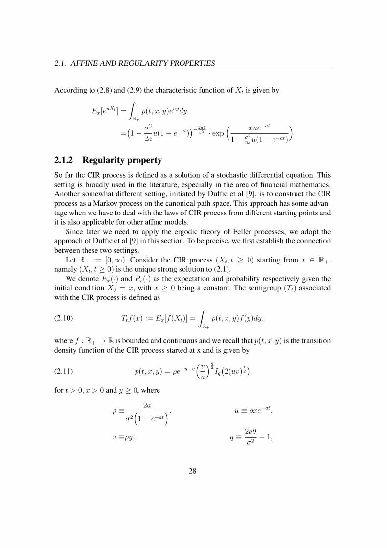
According to (2.8) and (2.9) the characteristic function of Xt is given by
Ex[euXt ] =
∫R+
p(t, x, y)euydy
=(1− σ2
2au(1− e−at)
)− 2aθσ2 · exp
( xue−at
1− σ2
2au(1− e−at)
)2.1.2 Regularity propertySo far the CIR process is defined as a solution of a stochastic differential equation. Thissetting is broadly used in the literature, especially in the area of financial mathematics.Another somewhat different setting, initiated by Duffie et al [9], is to construct the CIRprocess as a Markov process on the canonical path space. This approach has some advan-tage when we have to deal with the laws of CIR process from different starting points andit is also applicable for other affine models.
Since later we need to apply the ergodic theory of Feller processes, we adopt theapproach of Duffie et al [9] in this section. To be precise, we first establish the connectionbetween these two settings.
Let R+ := [0,∞). Consider the CIR process (Xt, t ≥ 0) starting from x ∈ R+,namely (Xt, t ≥ 0) is the unique strong solution to (2.1).
We denote Ex(·) and Px(·) as the expectation and probability respectively given theinitial condition X0 = x, with x ≥ 0 being a constant. The semigroup (Tt) associatedwith the CIR process is defined as
(2.10) Ttf(x) := Ex[f(Xt)] =
∫R+
p(t, x, y)f(y)dy,
where f : R+ → R is bounded and continuous and we recall that p(t, x, y) is the transitiondensity function of the CIR process started at x and is given by
(2.11) p(t, x, y) = ρe−u−v(vu
) q2Iq(2(uv)
12
)for t > 0, x > 0 and y ≥ 0, where
ρ ≡ 2a
σ2(
1− e−at) , u ≡ ρxe−at,
v ≡ρy, q ≡ 2aθ
σ2− 1,
28

2.1. AFFINE AND REGULARITY PROPERTIES
and Iq(·) is the first-order modified Bessel function with index q, defined by:
Iq(x) =(x
2
)q ∞∑k=0
(x2
)2k
k!Γ(q + k + 1).
For x = 0 the density function is given by
(2.12) p(t, 0, y) =ρ
Γ(q + 1)vqe−v
for t > 0 and y ≥ 0.
We write C0 = C0(R+) for the class of continuous functions which vanish at infinity.It is well-known that CIR process is an affine process (see [9]). It is already shown
in [9, Section 8] (see also [36]) that the semigroup of every stochastic continuous affineprocess is a Feller semigroup. Since CIR process is a diffusion process, it is obviouslystochastic continuous. Thus we know that (Tt)t≥0 defined in (2.10) is a Feller semigroup.
We denote the canonical path space by Ω, namely Ω = C([0,∞);R+
), and let
(Xt, t ≥ 0) be the canonical process on Ω. Let (Ft)t≥0 be the filtration generated by thecanonical process (Xt, t ≥ 0), namely Ft := σ(Xs, 0 ≤ s ≤ t) and F := σ(Xs, s ≥ 0).The map
X : (Ω,F)→ (Ω, F)
induces a measure Px on (Ω, F), which is the law of the CIR process starting fromx on the canonical path space. Since (Tt)t≥0 is Feller semigroup, the Markov process(Ω, F , Px, x ∈ R+) is a Feller process.
Following [29, Chapter 20] we give the definition of a regular Markov process on R+.
Definition 5. Consider a continuous-time Markov processZ with state space(R+,B(R+)
)and distributions Px. The process is said to be regular if there exist a locally finite mea-sure µ on R+ and a continuous function (t, x, y) 7→ p(t, x, y) > 0 on (0,∞) × R2
+ suchthat
PxZt ∈ B =
∫B
p(t, x, y)µ(dy), x ∈ R+, B ∈ B(R+), t > 0.
The measure µ is called the “supporting measure" of the process. It is unique up to anequivalence (see [29, page 399]).
Proposition 2. The CIR process is a regular Feller process on R+.
We will explain in the proof that the supporting measure can not be a Lebesgue mea-sure.
29

2.1. AFFINE AND REGULARITY PROPERTIES
Proof. As we have mentioned it before, the Feller property is already proved in [9, Section8]. We only need to prove the regularity property.
The modified Bessel functions of the first kind can be expanded as
Iq(r) =(r
2
)q ∞∑k=0
(14r2)k
k!Γ(q + k + 1)
thus has the following asymptotic forms
(2.13) Iq(r) =1
Γ(q + 1)
(r2
)q+O(rq+2)
for small arguments 0 < r √q + 1. If 2aθ
σ2 < 1, it follows that
p(t, x, 0) := limy→0
p(t, x, y) =∞, ∀x ∈ R+.
Thus (t, x, y) 7→ p(t, x, y) is not continuous on (0,∞)×R2+. On the other hand, if 2aθ
σ2 > 1,then we have
p(t, x, 0) := limy→0
p(t, x, y) = 0
Therefore in both cases the behavior of p(t, x, y) at point y = 0 violates the regularitycondition. To overcome this difficulty, we define a measure η on
(R+,B(R+)
)as
(2.14) η(dx) := h(x)dx,
where
h(x) =
x
2aθσ2−1, 0 ≤ x ≤ 1,
1, x > 1.
Then the transition density of the CIR process with respect to the new measure η is givenby
(2.15) p(t, x, y) =p(t, x, y)
h(y), t > 0, x ≥ 0, y > 0.
Recall that
ρ ≡ 2a
σ2(
1− e−at) , u ≡ ρxe−at,
v ≡ρy, q ≡ 2aθ
σ2− 1.
30

2.1. AFFINE AND REGULARITY PROPERTIES
At the point y = 0 we define
(2.16) p(t, x, 0) := limy→0
p(t, x, y) =1
Γ(q + 1)ρq+1e−u ∈ (0,∞)
From (2.15) we get
(2.17) 0 < p(t, x, y) <∞, t > 0, x ≥ 0, y > 0,
since h(y) and p(t, x, y) are positive and finite if y > 0. It follows from (2.16) and (2.17)that 0 < p(t, x, y) <∞ for all (t, x, y) ∈ (0,∞)× R2
+.Moreover, the function p(t, x, y) is continuous on (0,∞) × (0,∞) × (0,∞), which
follows from the continuity and positivity of the functions h(y) and p(t, x, y) with y > 0.Next we prove the continuity of p(t, x, y) at the point (0, 0, t0).
Let δ > 0 be sufficiently small. Then for |t− t0| ≤ δ and 0 ≤ x, y ≤ δ we have
|p(t, x, y)− p(t0, 0, 0)|≤|p(t, x, y)− p(t, 0, y)|+ |p(t, 0, y)− p(t, 0, 0)|+ |p(t, 0, 0)− p(t0, 0, 0)|
≤∣∣∣∣p(t, x, y)− p(t, 0, y)
h(y)
∣∣∣∣+
∣∣∣∣p(t, 0, y)
h(y)− p(t, 0, 0)
∣∣∣∣+ |p(t, 0, 0)− p(t0, 0, 0)|.(2.18)
By (2.11) and (2.13) we get∣∣∣∣p(t, x, y)− p(t, 0, y)
h(y)
∣∣∣∣=
1
|yq|
∣∣∣∣ρe−u−v(vu)q2( 1
Γ(q + 1)(uv)
q2 +O
((uv)
q2
+1))− ρ
Γ(q + 1)vqe−v
∣∣∣∣=
1
|yq|
∣∣∣∣ ρ
Γ(q + 1)e−v(e−u − 1
)vq +O
(uvq+1
)∣∣∣∣≤∣∣∣∣ ρq+1
Γ(q + 1)e−v(e−u − 1
)∣∣∣∣+O(uv).(2.19)
By (2.12) and (2.16) we have∣∣∣∣p(t, 0, y)
h(y)− p(t, 0, 0)
∣∣∣∣=
∣∣∣∣ ρvqe−v
Γ(q + 1)yq− 1
Γ(q + 1)ρq+1
∣∣∣∣ =
∣∣∣∣ ρq+1
Γ(q + 1)
(e−v − 1
)∣∣∣∣ .(2.20)
Since ρ is a continuous function with respect to the variable t, it follows from (2.16) that
(2.21) limt→t0|p(t, 0, 0)− p(t0, 0, 0)| = 0.
31

2.2. POSITIVE HARRIS RECURRENCE
It follows from (2.18), (2.19), (2.20) and (2.21) that
lim(t,x,y)→(t0,0,0)
|p(t, x, y)− p(t0, 0, 0)| = 0.
The continuity at other remaining points can be proved with a similar argument. Thus(t, x, y) 7→ p(t, x, y) is a positive continuous function on (0,∞)×R2
+. Therefore the CIRprocess is regular with respect to the measure η.
2.2 Positive Harris recurrenceIn this section we prove the main result of this chapter, namely we show that the CIRprocess, as a Feller process on R+, is positive Harris recurrent. Recall that (Ω, F , Px, x ∈R+) is the CIR process realized on the canonical path space. By (2.11) we know that
Px(Xt ∈ A) =
∫A
p(t, x, y)dy, ∀ A ∈ B(R+).
According to Proposition (2), we know that (Ω, Ft, Px, x ∈ R+) is a regular Feller processwith respect to the measure η defined in (2.14).
The stability and ergodic theory of continuous-time Markov processes has a largeliterature which includes many different approaches. For the readers we refer to [44, 45,46]. Recurrence theory permits us to establish stability even for models for which thestationary equations can not be explicitly solved (like the CIR process).
Let us first recall some basic definitions
Definition 6. A continuous-time Markov process Y on the state space(R+,B(R+)
)is
said to be Harris recurrent if for some σ-finite measure µ
(2.22) Px( ∫ ∞
0
1A(Ys)ds =∞)
= 1,
for any x ∈ R+ and A ∈ B(R+) with µ(A) > 0.
Definition 7. A continuous-time Markov process Y with state space(R+,B(R+)
)is said
to be uniformly transient if
(2.23) supxEx
[ ∫ ∞0
1K(Ys)ds]<∞
for every compact K ⊂ R+.
32

2.2. POSITIVE HARRIS RECURRENCE
Harris recurrence means that the Markov process (Yt, t ≥ 0) visit the Borel set A withµ(A) > 0 infinitely often. It was shown in [29, Theorem 20.17] that any Feller processis either Harris recurrent or uniformly transient. We are now ready to prove the positiverecurrence in the sense of Harris for the CIR process (Ω, F , Px, x ∈ R+).
Lemma 1. The CIR process (Ω, F , Px, x ∈ R+) is not uniformly transient.
Proof. We take K = [0,M ] with M > 0. Then for any fixed x ∈ (0,∞)
Ex
[ ∫ ∞0
1[0,M ](Xt)dt]
=
∫ ∞0
Ex[1[0,M ](Xt)
]dt
=
∫ ∞0
∫ M
0
p(t, x, y)dydt
=
∫ M
0
dy
∫ ∞0
p(t, x, y)dt.
The modified Bessel functions of the first kind have the following asymptotic forms, forsmall arguments 0 < r
√q + 1, one obtains
Iq(r) ≈1
Γ(q + 1)(r
2)q
where Γ denotes the Gamma function. Let ε > 0 be small enough. For any y ∈ [ε,M ] andlarge enough t we have
p(t, x, y) ≈ ρ
Γ(q + 1)e−ρy(ρy)q
and thus for y ∈ [ε,M ] ∫ ∞0
p(t, x, y)dt =∞.
It follows that
Ex
[ ∫ ∞0
1[0,M ](Xt)dt]
=
∫ M
0
dy
∫ ∞0
p(t, x, y)dt =∞.
This proves that the CIR process (Ω, F , Px, x ∈ R+) is not uniformly transient.
Harris recurrence guarantees the existence of a unique (up to multiplication by a con-stant) invariant measure for the Markov process (see e.g. [31]), but not necessarily finite.If this invariant measure is finite, then the process is called positive Harris recurrent.
Theorem 2. The CIR process (Ω, F , Px, x ∈ R+) is positive Harris recurrent.
33

2.3. ERGODICITY RESULTS
Proof. In Proposition (2) we have shown that the CIR process is a regular Feller processwith respect to the measure ρ defined in (2.14). It follows from Lemma 1 and [29, The-orem 20.17] that the CIR process is Harris recurrent and ρ can be taken as a possiblereference measure in place of µ in the Definition 6. Due to [29, Theorem 20.18] (see also[40, Theorem 1.3.5]) it is possible to construct a locally finite invariant measure µ for theCIR process. Furthermore µ is equivalent to ρ and every σ-finite, invariant measure for theCIR process agrees with µ up to a normalization. It was shown in [7] that µ is a Gammadistribution and has the form
(2.24) µ(dy) :=ων
Γ(ν)yν−1e−ωydy, y ≥ 0,
where ω ≡ 2aσ2 and ν ≡ 2aθ
σ2 . Thus the CIR process is positive Harris recurrent.
2.3 Ergodicity resultsAs a consequence of positive Harris recurrence we are able to prove the strong ergodicityof the CIR process. Based on Birkhoff’s ergodic theorem and the strong ergodicity wegive the ergodic results on transformation of the CIR.
Definition 8. (i) The tail σ-field on Ω is defined as T = ∩t≥0Tt, where Tt = σXs : s ≥t.(ii) A σ-field G ⊂ F on Ω is said to be Pν-trivial if Pν(A) = 0 or Pν(A) = 1 for everyA ∈ G, where Pν(·) :=
∫R+Px(·)ν(dx) denotes the distribution of the CIR process with
initial distribution ν.
From the positive Harris recurrence of the CIR process we reproduce the followingwell-known fact.
Corollary 1. The CIR process (Ω, F , Px, x ∈ R+) is strongly ergodic, meaning that thetail σ-field T of the CIR process is Pµ-trivial for every µ.
Proof. According to [29, Theorem 20.12] any Harris recurrent Feller process is stronglyergodic. From Theorem 2 we know that the CIR process (Ω, F , Px, x ∈ R+) is a stronglyergodic Markov process which means the tail σ-field T of the CIR process is Pµ-trivialfor every µ, see [29, Theorem 20.10].
34
2.3. ERGODICITY RESULTS
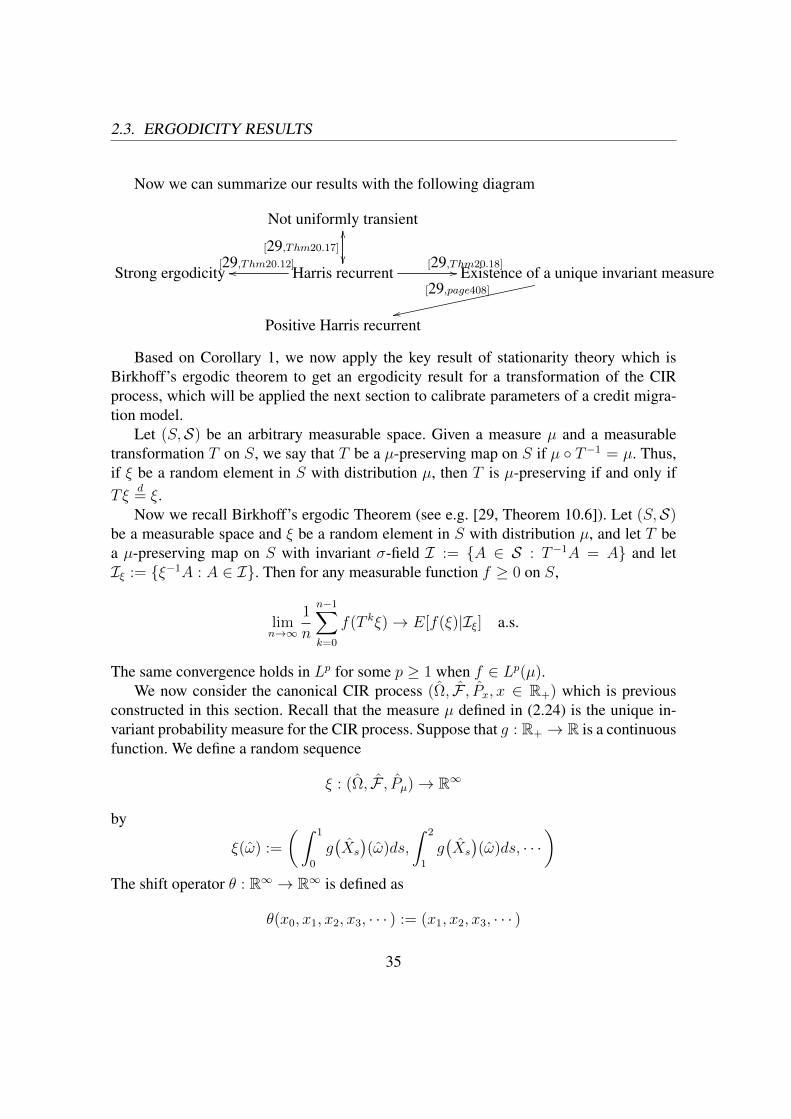
Now we can summarize our results with the following diagram
Not uniformly transient
[29,Thm20.17]
Strong ergodicity Harris recurrent[29,Thm20.12]oo
OO
[29,Thm20.18]// Existence of a unique invariant measure[29,page408]
rrPositive Harris recurrent
Based on Corollary 1, we now apply the key result of stationarity theory which isBirkhoff’s ergodic theorem to get an ergodicity result for a transformation of the CIRprocess, which will be applied the next section to calibrate parameters of a credit migra-tion model.
Let (S,S) be an arbitrary measurable space. Given a measure µ and a measurabletransformation T on S, we say that T be a µ-preserving map on S if µ T−1 = µ. Thus,if ξ be a random element in S with distribution µ, then T is µ-preserving if and only ifTξ
d= ξ.Now we recall Birkhoff’s ergodic Theorem (see e.g. [29, Theorem 10.6]). Let (S,S)
be a measurable space and ξ be a random element in S with distribution µ, and let T bea µ-preserving map on S with invariant σ-field I := A ∈ S : T−1A = A and letIξ := ξ−1A : A ∈ I. Then for any measurable function f ≥ 0 on S,
limn→∞
1
n
n−1∑k=0
f(T kξ)→ E[f(ξ)|Iξ] a.s.
The same convergence holds in Lp for some p ≥ 1 when f ∈ Lp(µ).We now consider the canonical CIR process (Ω, F , Px, x ∈ R+) which is previous
constructed in this section. Recall that the measure µ defined in (2.24) is the unique in-variant probability measure for the CIR process. Suppose that g : R+ → R is a continuousfunction. We define a random sequence
ξ : (Ω, F , Pµ)→ R∞
by
ξ(ω) :=
(∫ 1
0
g(Xs
)(ω)ds,
∫ 2
1
g(Xs
)(ω)ds, · · ·
)The shift operator θ : R∞ → R∞ is defined as
θ(x0, x1, x2, x3, · · · ) := (x1, x2, x3, · · · )
35

2.3. ERGODICITY RESULTS
for x = (x0, x1, x2, · · · ) and the invariant σ-field I on R∞ generated by the shift operatorθ is given by
I := A ∈ B(R∞) : θ−1A = A.
Lemma 2. Suppose that g : R+ → R is continuous and f : R→ R+ is measurable. Thenwe have
limN→∞
1
N
N−1∑j=0
f(∫ j+1
j
g(Xs
)(ω)ds
)= Eµ
[f(∫ 1
0
g(Xs
)ds)∣∣∣Iξ]
for Pµ-almost all ω ∈ Ω, where Iξ := ξ−1A : A ∈ I.
Proof. Since the initial distribution µ is an invariant measure for the CIR process
X1 ∼ µ.
It follows now from homogeneous Markov property that the random sequence ξ is sta-tionary, i.e.
θξd= ξ.
According to Birkhoff’s ergodic Theorem, for any measurable function h ≥ 0 on(R∞,B(R∞)
),
1
N
N−1∑i=0
h(θiξ)→ Eµ[h(ξ)|Iξ] a.s.
where Iξ := ξ−1I and I is the invariant σ-field on R∞ generated by the shift operator θ.Especially, if we take
h(x) := f(x0
)for x = (x0, x1, x2, · · · ) ∈ R∞, then we get
limN→∞
1
N
N−1∑j=0
f(∫ j+1
j
g(Xs
)(ω)ds
)= Eµ
[f(∫ 1
0
g(Xs
)ds)∣∣∣Iξ]
for Pµ-almost all ω ∈ Ω.
Lemma 3. The invariant σ-field Iξ of ξ is Pµ-trivial, namely
Pµ(A) = 0 or Pµ(A) = 1 for every A ∈ Iξ.
36

2.3. ERGODICITY RESULTS
Proof. Since Xt is continuous and g : R+ → R is continuous, thus
σ(ξj) = σ
(∫ j+1
j
g(Xs
)ds
)⊂ σX(s) : j ≤ s ≤ j + 1.
Thus the tail σ-field of the random sequence ξ is contained in the tail σ-field T of the CIRprocess Xt, where T = ∩t≥0Tt and Tt = σXs : s ≥ t. Because the invariant σ-field ofthe random sequence ξ is contained in the tail σ-field of ξ, we get Iξ ⊂ T . According toCorollary 1, the tail σ-field T of the CIR process Xt is Pµ-trivial, it follows that Iξ is alsoPµ-trivial.
Theorem 3. Suppose that g : R+ → R is continuous and f : R → R+ is measurable.Then for any x ∈ R+ we have
limN→∞
1
N
N−1∑j=0
f(∫ j+1
j
g(Xs
)(ω)ds
)= Eµ
[f(∫ 1
0
g(Xs
)(ω)ds
)]
for Px-almost all ω ∈ Ω, where µ is given (2.24)and is the unique invariant probabilitymeasure for the CIR process.
Proof. Since Iξ is Pµ-trivial, the conditional expectation
Eµ
[f(∫ 1
0
g(Xs
)ds)∣∣∣Iξ]
is a constant and equals
Eµ
[f(∫ 1
0
g(Xs
)ds)].
From Lemma 2 we get
(2.25) limN→∞
1
N
N−1∑j=0
f(∫ j+1
j
g(Xs
)(ω)ds
)= Eµ
[f(∫ 1
0
g(Xs
)ds)]
where the convergence in (2.25) holds for Pµ-almost all ω ∈ Ω. If we set
N :=ω ∈ Ω : the convergence in (2.25) fails for ω
,
thenPµ(N) =
∫R+
Px(N)µ(dx) = 0,
37

2.4. APPLICATION IN ONE CREDIT MIGRATION MODEL
which implies Px(N) = 0 for µ-almost all x ∈ R+. For any x ∈ R+, by the Markovproperty, it holds
Px(N) =Ex[1N ] = Ex[Ex[1N |F1]
]=Ex
[PX1
[θ−11 (N)]
]=
∫ ∞0
Py(N)p(1, x, y)dy
=0,
where p(t, x, y) denotes the transition density function of the CIR process. In the abovecalculation we have used the fact that θ−1
1 (N) = N , namely the pre-image of N under theshift operator θ is still N . Thus we have proved that the convergence in (2.25) holds forPx-almost all ω ∈ Ω.
2.4 Application in one credit migration modelIn this section we show a simple application of Theorem 3 in calibration of the parametersin one credit migration model. We should remark that the results presented in this sectionhave been derived in [39] with a different method. Their method is very analytical andrelies very much on the affine structure of the CIR process. In contrast to [39] our methodis more probabilistic and can be extended to more general models.
The idea of Hurd and Kuznetsov [22] was to generalize the 0 − 1 process to a finitestate Markov chain on 1, 2, · · · , k where each state represents credit rating or distanceto default of the firm. Here we consider a simpler version of the credit migration modelof Hurd and Kuznetsov where k = 8. Consider the finite state space 1, 2, · · · , 8, whichcan be identified with Moody’s rating classes via the mapping:
1, 2, · · · , 8 ↔ AAA, AA, A, BBB, BB, B, CCC, default.
The credit migration matrix P (s, t), 0 ≤ s ≤ t, is a stochastic 8× 8 matrix and describesall possible transition probabilities between rating classes from time s to time t, namely
(2.26) P (s, t) =(pij(s, t)
)1≤i,j≤8
where each pij(s, t) in (2.26) represents the transition probability from state i to statej from time s to time t. The last column of the migration matrix P (s, t) represents theabsorbing state of default, i.e. the probability of leaving the default state equals zero. Itwas assumed in [22] that the migration matrix P (s, t) is given by
(2.27) P (s, t) = exp
((∫ t
s
Xrdr)· P)
38

2.4. APPLICATION IN ONE CREDIT MIGRATION MODEL
where P is a 8× 8 constant matrix and Xt is a CIR process with long-term average 1,namely Xt satisfies
Xt = X0 +
∫ t
0
a(1−Xs)ds+
∫ t
0
σ√XsdWs, t ≥ 0
The matrix P is called the generator matrix. Thus the dynamics of the migration matrixis determined by two factors: the generator P and the CIR process Xt.
A natural question is how to calibrate the parameters of the above credit migrationmodel. More precisely, how can one determine the generator matrix P and the parametersa, θ, σ of the CIR process?
Among many other things, this problem was considered by [39] and they presented thefollowing way to calibrate the parameters of the above model, with extra assumptions onthe generator matrix P . The starting point is the Moody-matrix PMoody, which is derivedby Moody as the historical average of one year migration matrix, based on the historicaldata from 1920 to 1996. The logarithm matrix of PMoody is given by
(2.28) PMoody := log(PMoody) = log(id− (id− PMoody)) = −∞∑j=1
1
j(id− PMoody)
j
According to [24, Theorem 2.2], the right-hand side in (2.28) converges and thus PMoody
is well-defined andexp(PMoody) = PMoody
It was indicated by [39] that PMoody is diagonalizable and thus can be written as
(2.29) PMoody = G · (−DMoody,ii) ·G−1
where DMoody,ii is a diagonal matrix and G = (gik)1≤j,k≤8 is a matrix whose columns arethe corresponding eigenvectors of PMoody. Thus we get
PMoody = G · (e−DMoody,ii) ·G−1
Instead of finding a full 8 × 8 generator matrix, it was proposed in [39] to seek thegenerator matrix in the form
P = G · (−D) ·G−1
where D = (Dii) is a diagonal matrix with diagonal elements Dii ≥ 0 and G is given in(2.29).
39

2.4. APPLICATION IN ONE CREDIT MIGRATION MODEL
According to (2.27) the migration matrix from time j to j+ 1, j = 0, 1, 2, · · · is givenby
P (j, j + 1) = exp
((∫ j+1
j
Xsds)· P)
= G ·(e−Dii
∫ j+1j Xsds
)·G−1
= G ·
e−D11
∫ j+1j Xsds 0 · · · 0
0. . . ...
... . . . 0
0 · · · e−D88
∫ j+1j Xsds
·G−1
Thus the Cesàro average 1N
∑N−1j=0 P (j, j + 1) equals
(2.30) G ·
1N
∑N−1j=0 e−D11
∫ j+1j Xsds 0 · · · 0
0. . . ...
... . . . 0
0 · · · 1N
∑N−1j=0 e−D88
∫ j+1j Xsds
·G−1
For each 1 ≤ i ≤ 8 by taking g(x) = Diix and f(x) = e−x in Theorem 3 of lastsection we get
(2.31) limN→∞
1
N
N−1∑j=0
e−Dii∫ j+1j Xsds = Eµ
[e−Dii
∫ 10 Xsds
]and the convergence in (2.31) holds almost surely. Since each term under the limit sign onthe left hand side of (2.31) is bounded, by dominated convergence theorem, the conver-gence in (2.31) holds also in Lp for any p ≥ 1. We should remark that the L2 convergencein (2.31) was obtained in [39] with a different method. Our method used here is moreprobabilistic and provides us with a stronger convergence in (2.31).
Since the Laplace transform of∫ 1
0Xsds is well-known (for example, see [3, Lemma
2]), we getEx
[e−Dii
∫ 10 Xsds
]= eaA(0,Dii,1)+x·B(0,Dii,1)
40

2.4. APPLICATION IN ONE CREDIT MIGRATION MODEL
with deterministic functions
B(λ, u, t) := −λ(h− a+ (h+ a)e−ht) + 2u(1− e−ht)σ2λ(1− e−ht) + h+ a+ (h− a)e−ht
A(λ, u, t) :=2
σ2log
(2he
12
(a−h)t
σ2λ(1− e−ht) + h+ a+ (h− a)e−ht
)and h :=
√a2 + 2uσ2. Therefore
Eµ
[e−Dii
∫ 10 Xsds
]=
∫ ∞0
Ex
[e−Dii
∫ 10 Xsds
]µ(dx)
=
∫ ∞0
eaA(0,Dii,1)+x·B(0,Dii,1) ων
Γ(ν)xν−1e−ωxdx
=eaDiiA(0,Dii,1)( 2a
2a− σ2DiiB(0, Dii, 1)
) 2aσ2
.(2.32)
On the other hand PMoody is the historical average of one year migration matrix andthus it is reasonable to assume that
(2.33) PMoody = limN→∞
1
N
N−1∑j=0
P (j, j + 1),
if the limit on the right-hand side exists.It now follows from (2.30), (2.31), (2.32) and (2.33) that
(2.34) − DMoody,ii = aDiiA(0, Dii, 1) +2a
σ2log
(2a
2a− σ2DiiB(0, Dii, 1)
).
for each 1 ≤ i ≤ 8.To get more equations for the unknown parameters, we consider the probability of
rating downgrade from level A to the level BBB within time j und j + 1, which is givenby:
(2.35) p3,4(j, j + 1) :=8∑
k=1
g3k · e−Dkk∫ j+1j Xsds · gk4
where (gik)1≤i,k≤8 is the inverse of the matrix G. Similar to (2.31) we know that as N →∞
1
N
N−1∑j=0
p3,4(j, j + 1)
41

2.4. APPLICATION IN ONE CREDIT MIGRATION MODEL
converges almost surely to a constant, denoted by E3,4,∞, and we have
E3,4,∞ =8∑
k=1
g3keaDkkA(0,Dkk,1)
(2a
2a− σ2DkkB(0, Dkk, 1)
) 2aσ2
gk4
Define the ergodic variation
V3,4,∞ := limN→∞
1
N
N−1∑j=0
(p3,4(j, j + 1)− E3,4,∞
)2(2.36)
= limN→∞
1
N
N−1∑j=0
p23,4(j, j + 1)− E2
3,4,∞
Since
p23,4(j, j + 1) =
8∑i,k=1
g3ig3ke−(Dii+Dkk)
∫ j+1j Xsds · gi4gk4
it follows again from Theorem 3 that
limN→∞
1
N
N−1∑j=0
p23,4(j, j + 1) =
∑8i,k=1 g3ig3ke
(Dii+Dkk)aA(0,Dii+Dkk,1) ·
(2a
2a−σ2(Dii+Dkk)B(0,Dii+Dkk,1)
) 2aσ2
gi4gk4
Thus we get
VP,3,4,∞ =8∑
i,k=1
g3ig3ke(Dii+Dkk)aθA(0,Dii+Dkk,1)·
(2a
2a− σ2(Dii + Dkk)B(0, Dii + Dkk, 1)
) 2bσ2
gi4gk4−
8∑i,k=1
g3ig3keDiiaθA(0,Dii,1)+DkkaθA(0,Dkk,1)·
(2a
2a− σ2DiiB(0, Dii, 1)
) 2bσ2(
2a
2a− σ2DkkB(0, Dkk, 1)
) 2bσ2
gi4gk4(2.37)
42

2.4. APPLICATION IN ONE CREDIT MIGRATION MODEL
Based on the historical data from 1920 to 1996 Moody also gave the standard varia-tion of one year transition probabilities between different rating classes. For example thestandard variation of the one year transition probability from rating class A to BBB is0.053. We could approximately assume that this value coincides with the square of theergodic variation defined in (2.36), namely
(2.38) V3,4,∞ = (0.053)2.
Summarizing (2.34), (2.37) and (2.38) we get 9 equations for 10 unknown parameters.By fitting Moody’s standard variation of one year transition probability of another rat-ing transition we will get an extra equation. Thus all parameters of this migration matrixmodel can be uniquely determined by solving the 10 equations we have derived.
43
Chapter 3
Positive Harris recurrence, exponentialergodicity and calibration of the BAJD
In this chapter, we find the transition densities of the basic affine jump-diffusion (BAJD),which has been introduced by Duffie and Gârleanu as an extension of the classical CIRmodel with jumps. We prove the positive Harris recurrence and exponential ergodicity ofthe BAJD. Furthermore, we prove that the unique invariant probability measure π of theBAJD is absolutely continuous with respect to the Lebesgue measure and we also derivea closed form formula for the density function of π.
3.1 Characteristic function of the BAJDWe may now recall some preliminaries on the BAJD process. As defined in (1.7), it is theunique strong solution X = (Xt)t≥0 to the following stochastic differential equation
(3.1) dXt = a(θ −Xt)dt+ σ√XtdWt + dJt, X0 ≥ 0.
where a, θ, σ are positive constants, (Wt)t≥0 is a one-dimensional Brownian motion and(Jt)t≥0 is a one-dimensional non-decreasing pure jump Lévy process with identical inde-pendent increments, characterized by its jump measure ν which is supported on (0,∞).The Lévy measure ν is given by
ν(dy) =
cde−dydy, y ≥ 0,
0, y < 0,
for some constants c > 0 and d > 0. Throughout this chapter we denote Px(·) and Ex(·)as the probability and expectation respectively given the initial condition X0 = x, withx ≥ 0 being a constant.
44

3.1. CHARACTERISTIC FUNCTION OF THE BAJD
By the affine structure of the BAJD processX , the characteristic function ofXt (giventhat X0 = x) is of the form
(3.2) Ex[euXt
]= exp
(φ(t, u) + xψ(t, u)
), u ∈ U := u ∈ C : <u ≤ 0,
where the functions φ(t, u) and ψ(t, u) solve the generalized Riccati equations
(3.3)
∂tφ(t, u) = F
(ψ(t, u)
), φ(0, u) = 0,
∂tψ(t, u) = R(ψ(t, u)
), ψ(0, u) = u ∈ U ,
with
F (u) = aθu+cu
d− u, u ∈ C \ d,
R(u) =σ2u2
2− au, u ∈ C.
Remark that, it is not difficult to find the explicit form of the functions ∂tφ and ∂tψ. Wehave to proceed as in the Section (2.1). More precisely, we can find the functions ∂tφ and∂tψ under the initial conditions such that
Mt := f(t,Xt) = exp(φ(T − t, u) +Xtψ(T − t, u)
)is a martingale.
By applying Itô formula, one can get
(3.4)dM(t)
M(t)= −I(t)dt+ σψ(T − t, u)
√XtdWt +
∫(0,∞)
(eyψ(T−t,u) − 1
)ν(dy),
We can derive the generalized Riccati equation by collecting the coefficients.One can remark that the function R does not depend on the parameters of the jumps c andd. For this reason, the solution of the second equation of the system (3.3), ψ is the sameas in the case of classical CIR (2.8).
(3.5) ψ(t, u) =ue−at
1− σ2
2au(1− e−at)
Note that the first equation in the generalized Riccati equation is just an integral, andφ may be written explicitly as:
(3.6) φ(t, u) =
−2aθ
σ2 log(1− σ2
2au(1− e−at)
)+ c
a−σ2d2
log(d−σ
2du2a
+(σ2d2a−1)ue−at
d−u
), if ∆ 6= 0,
−2aθσ2 log
(1− σ2
2au(1− e−at)
)+ cu(1−e−at)
a(d−u), if ∆ = 0,
45

3.1. CHARACTERISTIC FUNCTION OF THE BAJD
where ∆ = a − σ2d/2. Here the complex-valued logarithmic function log(·) is to beunderstood as its main branch defined on C− 0.
According to (3.2), (3.5) and (3.6), the characteristic function of Xt is given by
(3.7) Ex[euXt ] =
(1− σ2
2au(1− e−at)
)− 2aθσ2 ·
(d−σ
2du2a
+(σ2d2a−1)ue−at
d−u
) c
a−σ2d2
· exp(
xue−at
1−σ22au(1−e−at)
), if ∆ 6= 0,(
1− σ2
2au(1− e−at)
)− 2aθσ2 · exp
(cu(1−e−at)a(d−u)
+ xue−at
1−σ22au(1−e−at)
),
if ∆ = 0.
Here the complex-valued power functions z−2aθ/σ2:= exp(−(2aθ/σ2) log z) and zc/(a−σ2d/2) :=
exp((c log z)/(a−σ2d/2)) are to be understood as their main branches defined on C−0.ObviouslyEx
[exp(uXt)
]is continuous in t ≥ 0 and thus the BAJD processX is stochas-
tically continuous.We should point out that if we allow the parameter c to be 0, then the stochastic
differential equation (3.1) turns into
(3.8) dZt = a(θ − Zt)dt+ σ√ZtdWt, Z0 = x ≥ 0.
To avoid confusions we have usedZt instead ofXt here. The unique solutionZ := (Zt)t≥0
to (3.8) is the well-known Cox-Ingersoll-Ross (CIR) process and it holds
(3.9) Ex[euZt ] =
(1− σ2
2au(1− e−at)
)− 2aθσ2 · exp
( xue−at
1− σ2
2au(1− e−at)
).
Later we will find a distribution νt on R+ such that
(3.10)∫R+
euyνt(dy) =
(d−σ
2du2a
+(σ2d2a−1)ue−at
d−u
) c
a−σ2d2 , if ∆ 6= 0,
exp(cu(1−e−at)a(d−u)
), if ∆ = 0.
Then it follows from (3.7), (3.9) and (3.10) that the distribution of the BAJD is the con-volution of the distribution of the CIR process and νt. In light of this observation we canthus identify the transition probabilities p(t, x, y) of the BAJD with
(3.11) p(t, x, y) =
∫R+
f(t, x, y − z)νt(dz), x, y ≥ 0, t > 0,
to avoid confusion we have used f instead of p, where f(t, x, y) denotes the transitiondensities of the CIR process.Remark 4. For a different way of representing the distribution of Xt as a convolution werefer the reader to [13]. In fact it was indicated in [13, Remark 4.8] that the distributionof any affine process on R+ can be represented as the convolution of two distributions onR+.
46

3.2. MIXTURES OF BESSEL DISTRIBUTIONS
3.2 Mixtures of Bessel distributionsTo find a distribution νt with the characteristic function of the form (3.10) and study thedistributional properties of the BAJD, it is inevitable to encounter the Bessel distributionsand mixtures of Bessel distributions.
We start with a slight variant of the Bessel distribution defined in [19, p.15]. Supposethat α and β are positive constants. A probability measure µα,β on
(R+,B(R+)
)is called
a Bessel distribution with parameters α and β if
(3.12) µα,β(dx) = e−αδ0(dx) + βe−α−βx√
α
βx· I1(2
√αβx)dx,
where δ0 is the Dirac measure at the origin and I1 is the modified Bessel function of thefirst kind, namely,
I1(r) =r
2
∞∑k=0
(14r2)k
k!(k + 1)!, r ∈ R.
Now we consider mixtures of Bessel distributions. Let γ > 0 be a constant and definea probability measure mα,β,γ on R+ as follows:
mα,β,γ(dx) :=
∫ ∞0
µαt,β(dx)tγ−1
Γ(γ)e−tdt.
Similar to [19], we can easily calculate the characteristic function of µα,β and mα,β,γ .
Lemma 4. For u ∈ U we have:
(i)∫ ∞
0
euxµα,β(dx) = eαuβ−u .
(ii)∫ ∞
0
euxmα,β,γ(dx) =( 1
α + 1+
α
α + 1· 1
1− α+1β· u
)γ.
47

3.2. MIXTURES OF BESSEL DISTRIBUTIONS
Proof. (i) If u ∈ U , then∫ ∞0
euxµα,β(dx) =
∫ ∞0
euxe−αδ0(dx) +
∫ ∞0
βeuxe−α−βx√
α
βx· I1(2
√αβx)dx
=e−α + e−α∫ ∞
0
βe−βx · eux√
α
βx
(√αβx
)·∞∑k=0
(αβx)k
k!(k + 1)!dx
=e−α + e−α∫ ∞
0
αβe(u−β)x ·∞∑k=0
(αβx)k
k!(k + 1)!dx
=e−α + αβe−α∞∑k=0
∫ ∞0
e(u−β)x (αβx)k
k!(k + 1)!dx
=e−α + e−α∞∑k=0
( αβ
β − u
)k+1
· 1
(k + 1)!
=e−α∞∑k=0
( αβ
β − u
)k· 1
k!= e−α · e
αββ−u = e
αuβ−u .
(ii) For u ∈ U , we get∫ ∞0
euxmα,β,γ(dx) =
∫ ∞0
(
∫ ∞0
euxµαt,β(dx))tγ−1
Γ(γ)e−tdt
=
∫ ∞0
eαt·u
β−u · tγ−1
Γ(γ)e−tdt =
(1 + α · u
u− β
)−γ=
(−β + (α + 1)u
−β + u
)−γ=( −β + u
−β + (α + 1)u
)γ=
( 1α+1
((α + 1)u− β) + βα+1− β
−β + (α + 1)u
)−γ=
( 1
α + 1+
α
α + 1· 1
1− α+1β· u
)γ.(3.13)
Lemma 5. (i) The measure mα,β,γ can be represented as follows:
(3.14) mα,β,γ(dx) =( 1
1 + α
)γδ0 + gα,β,γ(x)dx, x ≥ 0,
where
(3.15) gα,β,γ(x) :=∞∑k=1
αkΓ(k + γ)
(α + 1)k+γΓ(γ)k!Γ(x; k, β), x ≥ 0,
48

3.2. MIXTURES OF BESSEL DISTRIBUTIONS
and Γ(x; k, β) denotes the density function of the Gamma distribution with parameters kand β.(ii) The function gα,β,γ(x) defined in (3.15) is a continuous function with variables (α, β, γ, x) ∈D := (0,∞)× (0,∞)× (0,∞)× [0,∞).
Proof. (i) We can write
mα,β,γ(dx) =
∫ ∞0
µαt,β(dx)tγ−1
Γ(γ)e−tdt
=
∫ ∞0
(e−αtδ0(dx) + βe−αt−βx
√αt
βx· I1(2
√αtβx)dx
) tγ−1
Γ(γ)e−tdt
=( 1
1 + α
)γδ0(dx) +
∫ ∞0
αβe−αt−βx∞∑k=0
(αtβx)k
k!(k + 1)!· tγ
Γ(γ)e−tdtdx
=( 1
1 + α
)γδ0(dx) + αβe−βx ·
∞∑k=0
(∫ ∞0
(αβx)ke−(α+1)ttγ+k
Γ(γ)k!(k + 1)!dt)dx
=( 1
1 + α
)γδ0(dx) +
∞∑k=0
αk+1Γ(k + γ + 1)
(α + 1)k+γ+1Γ(γ)(k + 1)!Γ(x; k + 1, β)dx
=( 1
1 + α
)γδ0(dx) +
∞∑k=1
αkΓ(k + γ)
(α + 1)k+γΓ(γ)k!Γ(x; k, β)dx.
(ii) By the definition of gα,β,γ(x) we have
gα,β,γ(x) =
∫ ∞0
βe−αt−βx√αt
βx· I1(2
√αtβx)
tγ−1
Γ(γ)e−tdt
=
∫ ∞0
αβe−αt−βx( ∞∑k=0
(αtβx)k
k!(k + 1)!
) tγ
Γ(γ)e−tdt
=
∫ ∞0
αβtγ
Γ(γ)e−(α+1)t−βx( ∞∑
k=0
(αtβx)k
k!(k + 1)!
)dt
Suppose that (α0, β0, γ0, x0) ∈ D and δ > 0 is small enough such that γ0 − δ > 0,α0 − δ > 0 and β0 − δ > 0. Then for (α, β, γ, x) ∈ Kδ with
Kδ := (α, β, γ, x) ∈ D : max|α− α0|, |β − β0|, |γ − γ0|, |x− x0| ≤ δ
49

3.3. TRANSITION DENSITY OF THE BAJD
we get
αβtγ
Γ(γ)e−(α+1)t−βx( ∞∑
k=0
(αtβx)k
k!(k + 1)!
)≤αβt
γ
Γ(γ)e−(α+1)t−βx( ∞∑
k=0
(αt)k(βx)k
(k!)2
)≤αβt
γ
Γ(γ)e−(α+1)t−βx · eαteβx ≤ αβtγ
Γ(γ)e−t
≤cδ(tγ0−δ1[0,1](t) + tγ0+δe−t1(1,∞)(t)
)(3.16)
for some constant cδ > 0, since αβΓ(γ)
is continuous and thus bounded for(α, β, γ, x) ∈ Kδ. If (αn, βn, γn, xn) → (α0, β0, γ0, x0) as n → ∞, then by dominatedconvergence we get
limn→∞
gαn,βn,γn(xn) = gα0,β0,γ0(x0),
namely gα,β,γ(x) is a continuous function on D.
Remark 5. If we write δ0 = Γ(0, β), namely considering the Dirac measure δ0 as a de-generated Gamma distribution, then the representation in (3.14) shows that the measuremα,β,γ is a mixture of Gamma distributions Γ(k, β), k ∈ Z+, namely
mα,β,γ =( 1
1 + α
)γΓ(0, β) +
∞∑k=1
αkΓ(k + γ)
(α + 1)k+γΓ(γ)k!Γ(k, β).
3.3 Transition density of the BAJDIn this section we shall derive a closed form expression for the transition density of theBAJD. We should mention that in [13, Chapter 7] the density functions of the pricingsemigroup associated to the BAJD was derived for some special cases. Essentially, themethod used in [13] could be used to derive the density functions of the BAJD in thecase where c/(a − σ2d/2) ∈ Z. Here we proceed like [13] but deal with more generalparameters. In order to do this, we first find, by using the results of the previous section,a probability measure νt on R+ whose characteristic function satisfies (3.10).
We recall that the BAJD process X = (Xt)t≥0 is given by (3.1). We distinguish be-tween three cases according to the sign of ∆ := a− σ2d/2.
50
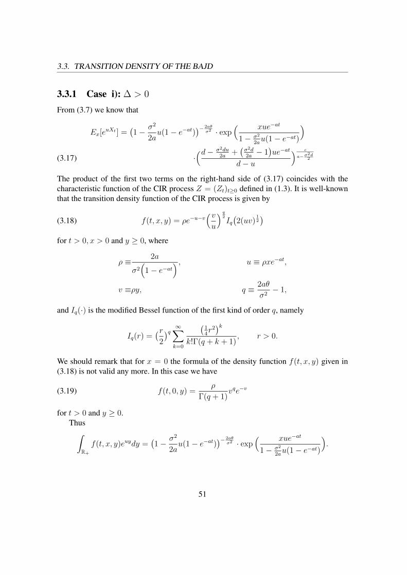
3.3. TRANSITION DENSITY OF THE BAJD
3.3.1 Case i): ∆ > 0
From (3.7) we know that
Ex[euXt ] =
(1− σ2
2au(1− e−at)
)− 2aθσ2 · exp
( xue−at
1− σ2
2au(1− e−at)
)·(d− σ2du
2a+(σ2d2a− 1)ue−at
d− u
) c
a−σ2d2(3.17)
The product of the first two terms on the right-hand side of (3.17) coincides with thecharacteristic function of the CIR process Z = (Zt)t≥0 defined in (1.3). It is well-knownthat the transition density function of the CIR process is given by
(3.18) f(t, x, y) = ρe−u−v(vu
) q2Iq(2(uv)
12
)for t > 0, x > 0 and y ≥ 0, where
ρ ≡ 2a
σ2(
1− e−at) , u ≡ ρxe−at,
v ≡ρy, q ≡ 2aθ
σ2− 1,
and Iq(·) is the modified Bessel function of the first kind of order q, namely
Iq(r) =(r
2
)q ∞∑k=0
(14r2)k
k!Γ(q + k + 1), r > 0.
We should remark that for x = 0 the formula of the density function f(t, x, y) given in(3.18) is not valid any more. In this case we have
(3.19) f(t, 0, y) =ρ
Γ(q + 1)vqe−v
for t > 0 and y ≥ 0.Thus∫
R+
f(t, x, y)euydy =(1− σ2
2au(1− e−at)
)− 2aθσ2 · exp
( xue−at
1− σ2
2au(1− e−at)
).
51
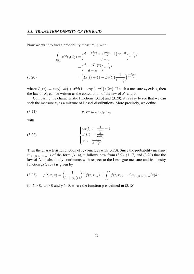
3.3. TRANSITION DENSITY OF THE BAJD
Now we want to find a probability measure νt with∫R+
euyνt(dy) =(d− σ2du
2a+(σ2d2a− 1)ue−at
d− u
) c
a−σ2d2
=(d− uL1(t)
d− u
) c
a−σ2d2
=(L1(t) +
(1− L1(t)
) 1
1− ud
) c
a−σ2d2 ,(3.20)
where L1(t) := exp(−at) + σ2d(1 − exp(−at)
)/(2a). If such a measure νt exists, then
the law of Xt can be written as the convolution of the law of Zt and νt.Comparing the characteristic functions (3.13) and (3.20), it is easy to see that we can
seek the measure νt as a mixture of Bessel distributions. More precisely, we define
(3.21) νt := mα1(t),β1(t),γ1
with
(3.22)
α1(t) := 1
L1(t)− 1
β1(t) := dL1(t)
γ1 := c
a−σ2d2
.
Then the characteristic function of νt coincides with (3.20). Since the probability measuremα1(t),β1(t),γ1 is of the form (3.14), it follows now from (3.9), (3.17) and (3.20) that thelaw of Xt is absolutely continuous with respect to the Lesbegue measure and its densityfunction p(t, x, y) is given by
(3.23) p(t, x, y) =( 1
1 + α1(t)
)γ1f(t, x, y) +
∫ y
0
f(t, x, y − z)gα1(t),β1(t),γ1(z)dz
for t > 0, x ≥ 0 and y ≥ 0, where the function g is defined in (3.15).
52

3.3. TRANSITION DENSITY OF THE BAJD
3.3.2 Case ii): ∆ < 0
Similar to the case (i), it suffices to find a probability measure νt with∫R+
euyνt(dy) =(d− σ2du
2a+(σ2d2a− 1)ue−at
d− u
) c
a−σ2d2
=( d− ud− σ2du
2a+(σ2d2a− 1)ue−at
) −ca−σ2d
2
=( d− ud− L1(t)u
) −ca−σ2d
2
=
(1
L1(t)+ (1− 1
L1(t)) · 1
1− L1(t)ud
) −ca−σ2d
2 .(3.24)
Since ∆ = a− σ2d/2 < 0, therefore σ2d/2a > 1 and
L1(t) = e−at +σ2d
2a·(1− e−at
)> 1.
According to the formula (3.12), we can choose
νt = mα2(t),β2(t),γ2
with the parameters α2, β2 and γ2 defined by
(3.25)
α2(t) := L1(t)− 1
β2 := d
γ2 := −ca−σ2d
2
.
Similar to the case (i), the transition densities p(t, x, y) of X is given by
(3.26) p(t, x, y) =( 1
1 + α2(t)
)γ2f(t, x, y) +
∫ y
0
f(t, x, y − z)gα2(t),β2,γ2(z)dz
for t > 0, x ≥ 0 and y ≥ 0, where the function g is defined in (3.15).
3.3.3 Case iii): ∆ = 0
In this case we need to find a probability measure νt with∫R+
euyνt(dy) = exp(cu(1− e−at)
a(d− u)
).
53

3.3. TRANSITION DENSITY OF THE BAJD
According to the formula (3.14) we can take νt as a Bessel distribution µα3(t),β3 with theparameters α3(t) and β3 defined by
(3.27)
α3(t) := c
a(1− e−at)
β3 := d.
Thus in this case the transition densities p(t, x, y) of X is given by
p(t, x, y) =
∫ y
0
f(t, x,y − z)β3e−α3(t)−β3z
√α3(t)
β3zI1(2
√α3(t)β3z)dz
+e−α3(t)f(t, x, y)(3.28)
for t > 0, x ≥ 0 and y ≥ 0.Summarizing the above three cases we get the following theorem.
Theorem 6. Let X = (Xt)t≥0 be the BAJD defined in (3.1). Then the law of Xt giventhat X0 = x ≥ 0 is absolutely continuous with respect to the Lesbegue measure and thuspossesses a density function p(t, x, y), namely
Px(Xt ∈ A) =
∫A
p(t, x, y)dy, t ≥ 0, A ∈ B(R+)
According to the sign of ∆ = a − σ2d/2, the density p(t, x, y) is given by (3.23), (3.26)and (3.28) respectively.
Although the density functions in (3.23), (3.26) and (3.28) are essentially different,they do share some similarities. In the following corollary we give a unified representationof p(t, x, y).
Corollary 2. Irrelevant of the the sign of ∆ = a−σ2d/2, the transition densities p(t, x, y)of X can be expressed in a unified form as
(3.29) p(t, x, y) = L(t)f(t, x, y) +
∫ y
0
f(t, x, y − z)h(t, z)dz,
where L(t) is continuous function in t > 0 which satisfies 0 < L(t) < 1 for t > 0, thefunction h(t, z) is non-negative and continuous in (t, z) ∈ (0,∞) × [0,∞) and satisfies∫R+h(t, z)dz = 1− L(t).
54

3.4. POSITIVE HARRIS RECURRENCE OF THE BAJD
3.4 Positive Harris recurrence of the BAJDIt was shown in [9] (see also [36]) that the semigroup of any stochastically continuousaffine process on the canonical state space Rm
+ × Rn is a Feller semigroup. Define thesemigroup of the BAJD by
(3.30) Ttf(x) :=
∫R+
p(t, x, y)f(y)dy,
where f : R+ → R is bounded. Since the BAJD process X is stochastically continuousand affine, thus (Tt)t≥0 is a Feller semigroup.
To show the positive Harris recurrence, we need first to prove the regularity propertyof BAJD. To this aim, we first analyse the continuity properties of the integral whichappears on the right hand side of (3.29).
Lemma 6. Let f(t, x, y) be the transition density of the CIR process given in (3.18) andh(t, z) be the same as in (3.29). Then the function F (t, x, y) defined by
(3.31) F (t, x, y) :=
∫ y
0
f(t, x, y − z)h(t, z)dz
is continuous with variables (t, x, y) ∈ (0,∞)× [0,∞)× [0,∞). Moreover if M > 1 isa constant, then
(3.32) |F (t, x, y)| ≤ Cy2aθσ2
for all
(t, x, y) ∈ KM := (t, x, y) :1
M≤ t ≤M, 0 ≤ x ≤M, 0 ≤ y ≤ 1
M,
where C > 0 is a constant which depends on M .
Proof. For simplicity we set q := 2aθ/σ2 − 1 as in (3.18). Since h(t, z) is continuous in(t, z) ∈ (0,∞)× [0,∞), thus there exists a constant c1 > 0 depending on M such that
(3.33) |h(t, z)| ≤ c1 for1
M≤ t ≤M, 0 ≤ z ≤ 1
M.
Therefore if (t, x, y) ∈ KM , we have
(3.34) |F (t, x, y)| ≤ c1
∫ y
0
f(t, x, y − z)dz.
55

3.4. POSITIVE HARRIS RECURRENCE OF THE BAJD
According to (3.18) and (3.19) we have
(3.35) |f(t, x, y − z)| ≤ c2|y − z|q if (t, x, y − z) ∈ KM and y 6= z,
where c2 > 0 is a constant depending on M .It follows from (3.34) and (3.35) that
(3.36) |F (t, x, y)| ≤ c1c2
∫ y
0
|y − z|qdz =c1c2
q + 1yq+1 ≤ c3y
q+1
for (t, x, y) ∈ KM , if we set c3 := c1c2/(q + 1). Thus (3.32) is proved. Noting thatF (t, x, 0) = 0 for t > 0 and x ≥ 0, the continuity of the function F at points (t, x, 0) isan immediate consequence of the estimate (3.36).We now proceed to prove the continuity of F at other points. Suppose that t0 > 0, x0 ≥ 0and y0 > 0 are fixed. Let ε > 0 be arbitrary. We choose δ1 > 0 small enough such thaty0 − 2δ1 > 0 and t0 − δ1 > 0. As in (3.33) and (3.35) there exist constants c4, c5 > 0,which depend on δ1, such that
(3.37) |h(t, z)| ≤ c4 for t ∈ [t0 − δ1, t0 + δ1], z ∈ [0, y0 + δ1]
and
(3.38) |f(t, x, y − z)| ≤ c5|y − z|q
for t ∈ [t0 − δ1, t0 + δ1], x ∈ [0, x0 + δ1] and 0 < y − z ≤ y0 + δ1. Set
Kδ2 := [t0 − δ2, t0 + δ2]× [0, x0 + δ2]× [y0 − δ2, y0 + δ2].
We choose δ2 > 0 small enough such that δ2 < δ1 and c4c5(3δ2)q+1/(q + 1) < ε/3. If(t, x, y) ∈ Kδ2 then it holds∣∣∣ ∫ y
y0−2δ2
f(t, x, y − z)h(t, z)dz∣∣∣ ≤ c4c5
∫ y
y0−2δ2
(y − z)qdz
=c4c5
q + 1(y − y0 + 2δ2)q+1
≤ c4c5
q + 1(3δ2)q+1 <
ε
3.(3.39)
If (t, x, y) ∈ Kδ2 and 0 ≤ z ≤ y0 − 2δ2, then δ2 ≤ y − z ≤ y0 + δ2 and by (3.37) and(3.38) we have
|f(t, x, y − z)h(t, z)| ≤ c4c5|y − z|q
≤ c4c5(|δ2|q + |y0 + δ2|q).(3.40)
56

3.4. POSITIVE HARRIS RECURRENCE OF THE BAJD
Since for fixed z ∈ [0, y0−2δ2] the function f(t, x, y−z)h(t, z) is continuous in (t, x, y) ∈Kδ2 , it follows from (3.40) and dominated convergence theorem that
F2(t, x, y) :=
∫ y0−2δ2
0
f(t, x, y − z)h(t, z)dz
is a continuous function in (t, x, y) ∈ Kδ2 . This implies the existence of a constant δ with0 < δ < δ2 such that
(3.41) |F2(t, x, y)− F2(t0, x0, y0)| < ε
3,
if (t, x, y) ∈ Kδ := [t0 − δ, t0 + δ] × [0 ∨ (x0 − δ), x0 + δ] × [y0 − δ, y0 + δ]. Thus itfollows from (3.39) and (3.41) that
|F (t, x, y)− F (t0, x0, y0)| < ε
for (t, x, y) ∈ Kδ. The continuity of the function F at (t0, x0, y0) is proved.
According to (3.29) and Lemma 6, the boundary behavior of the transition densitiesp(t, x, y) of X at y = 0 depends very much on the behavior of f(t, x, y) at y = 0. Asshown in the proof of proposition 2 of chapter 2, if 2aθ/σ2 < 1, then
f(t, x, 0) := limy→0
f(t, x, y) =∞, ∀x ∈ R+,
which means that (t, x, y) 7→ f(t, x, y) is not continuous on (0,∞)×R2+; if 2aθ/σ2 > 1,
thenf(t, x, 0) := lim
y→0f(t, x, y) = 0.
Therefore, in both cases the behavior of f(t, x, y) at the boundary y = 0 violates theregularity condition; as a consequence, the transition densities p(t, x, y) of X are also notregular. To overcome this difficulty, we proceed as in the proof of proposition 2 of chapter2 and define a new measure η on
(R+,B(R+)
)as
(3.42) η(dx) := κ(x)dx,
where
κ(x) =
x
2aθσ2−1, 0 ≤ x ≤ 1,
1, x > 1.
Then the transition densities of the BAJD process with respect to the new measure η isgiven by
(3.43) p(t, x, y) =p(t, x, y)
κ(y), t > 0, x ≥ 0, y > 0.
57

3.4. POSITIVE HARRIS RECURRENCE OF THE BAJD
Theorem 7. The transition densities p(t, x, y) of the BAJD process with respect to themeasure η satisfies
0 < p(t, x, y) <∞, t > 0, x ≥ 0, y ≥ 0
and is continuous in (t, x, y) ∈ (0,∞) × [0,∞) × [0,∞). Thus the BAJD is a regularFeller process on the state space R+.
For the definition of regular continuous-time Markov process we refer to the definition(5) of Chapter 2.
Proof. From (3.29) we can write the transition density of the BAJD process with respectto the measure η as
p(t, x, y) = L(t)f(t, x, y)
κ(y)+F (t, x, y)
κ(y)
= L(t)f(t, x, y) +F (t, x, y)
κ(y)(3.44)
where f(t, x, y) is the transition density of CIR with respect the new measure η and F isdefined in (3.31). We have already shown in Proposition 2 of Chapter 2 that
(3.45) 0 < f(t, x, y) <∞, t > 0, x ≥ 0, y ≥ 0,
and (t, x, y) 7→ f(t, x, y) is a continuous function on (0,∞)× R2+.
From Lemma 6, we know that the function F (t, x, y) appearing in the second summandin (3.44) is continuous on (0,∞)× R2
+ and
|F (t, x, y)| ≤ Cy2aθσ2 , if (t, x, y) ∈ KM ,
where C > 0 is a constant depending on M . Now it is clear that
0 ≤ limy→0
F (t, x, y)
κ(y)≤ lim
y→0C|y| = 0.
Since F (t, x, 0) = 0 and L(t) is continuous in t > 0, it follows that the function p(t, x, y)is continuous at points (t0, x0, 0), if t0 > 0 and x0 ≥ 0. The continuity of the functionp(t, x, y) at other points is also clear, because all the functions appearing in (3.44) arecontinuous and 0 < κ(y) <∞ for y > 0. Noting that 0 < L(t) < 1 for t > 0, we get
0 < p(t, x, y) <∞ for all (t, x, y) ∈ (0,∞)× R2+.
Therefore the BAJD process is a regular Feller process with η as the supporting measure.
58

3.4. POSITIVE HARRIS RECURRENCE OF THE BAJD
Let us recall the following definitions from Chapter 2, we refer to [45, p.490] and [29,p.405].
Definition 9. Consider a time-homogeneous Markov process Y = (Yt)t≥0 with the statespace R+ and distributions Px, x ∈ R+.(i) Y is said to be Harris recurrent if for some σ-finite measure µ
(3.46) Px( ∫ ∞
0
1A(Ys)ds =∞)
= 1,
for any x ∈ R+ and A ∈ B(R+) with µ(A) > 0. It was shown in [16] that if Y is Harrisrecurrent then it possesses a unique (up to a renormalization) invariant measure. If theinvariant measure is finite, then the process Y is called positive Harris recurrent.(ii) Y is said to be uniformly transient if
(3.47) supxEx
[ ∫ ∞0
1K(Ys)ds]<∞
for every compact K ⊂ R+.
Lemma 7. The BAJD is not uniformly transient.
Proof. Let m > 0, K := [0,m] and x ∈ (0,∞) be fixed. Then
Ex
[ ∫ ∞0
1[0,m](Xt)dt]
=
∫ ∞0
Ex[1[0,m](Xt)
]dt
=
∫ ∞0
∫ m
0
p(t, x, y)dydt
=
∫ m
0
dy
∫ ∞0
p(t, x, y)dt.
From (3.29) and (3.31) we know that
p(t, x, y) = L(t)f(t, x, y) + F (t, x, y).
It follows from (3.23), (3.26) and (3.28) that
(3.48) 0 < limt→∞
L(t) =
(σ2d2a
) c
a−σ2d2 , if ∆ 6= 0,
e−ca , if ∆ = 0.
Since F (t, x, y) is non-negative, thus there exists large enough T > 0 such that
p(t, x, y) ≥ λf(t, x, y) for t ≥ T,
59

3.4. POSITIVE HARRIS RECURRENCE OF THE BAJD
where λ > 0 is a constant. Let ε > 0 be small enough. According to Lemma 1 of Chapter2 we know that for any x > 0 and y ∈ [ε,m] it holds∫ ∞
0
f(t, x, y)dt =∞.
Therefore
Ex
[ ∫ ∞0
1[0,m](Xt)dt]
=
∫ m
0
dy
∫ ∞0
p(t, x, y)dt
≥∫ m
ε
dy
∫ ∞R
λf(t, x, y)dt =∞.
This proves that the BAJD is not uniformly transient.
Theorem 8. The BAJD is Harris recurrent.
Proof. We have shown that the BAJD is a regular Feller process with the measure η,which is defined in (3.42), as a supporting measure. It follows from Lemma 7 and [29,Theorem 20.17] that the BAJD is Harris recurrent and the measure η satisfies (3.46).
Remark 9. Since the BAJD is a Harris recurrent Feller process, it follows from [29, The-orem 20.18] that the BAJD has a locally finite invariant measure π which is equivalent tothe supporting measure η. Moreover every σ -finite invariant measure of the BAJD agreeswith π up to a renormalization. The existence and uniqueness of an invariant probabilitymeasure for the BAJD has already been proved in [32] (see also [38]). Thus we can as-sume π to be a probability measure. The characteristic function of π was given in [38]and has the form
(3.49)∫R+
euzπ(dz) =
(1− σ2
2au)− 2aθ
σ2 ·(d−σ
2du2a
d−u
) c
a−σ2d2 , if ∆ 6= 0,(
1− σ2
2au)− 2aθ
σ2 · exp(
cua(d−u)
), if ∆ = 0.
Corollary 3. The BAJD is positive Harris recurrent. Its unique invariant probability mea-sure π is absolute continuous with respect to the Lebesgue measure and thus has a densityfunction l(·), namely π(dy) = l(y)dy, y ∈ R+. If ∆ 6= 0, then we have
l(y) =(σ2d
2a
) c
a−σ2d2 Γ(y;
2aθ
σ2,σ2
2a
)+
∫ y
0
Γ(y − z;
2aθ
σ2,σ2
2a
)h(z)dz, y ≥ 0,
where Γ(y; 2aθ/σ2, σ2/(2a)
)denotes the density function of the Gamma distribution with
parameters 2aθ/σ2 and σ2/(2a), and
h(z) =
g 2aσ2d−1, 2a
σ2, c
a−σ2d2
(z), if ∆ > 0,
gσ2d2a−1,d,− c
a−σ2d2
(z), if ∆ < 0,
60

3.5. EXPONENTIAL ERGODICITY OF THE BAJD
with g defined in (3.15). If ∆ = 0, then we have
l(y) = e−caΓ(y;
2aθ
σ2,σ2
2a
)+
∫ y
0
Γ(y − z;
2aθ
σ2,σ2
2a
)de−
ca−dz√
c
adz· I1
(2
√cdz
a
)dz
for y ≥ 0.
Proof. We apply the same method which we used in Section 3.3 to find the transitiondensities of the BAJD. Since the characteristic function of π is given by (3.49) and notingthat the first term on the right hand side of (3.49) corresponds to the characteristic functionof a Gamma distribution, we can represent the measure π as a convolution of a Gammadistribution with a probability measure ν. If ∆ = 0 the measure ν is a Bessel distribution,otherwise it is a mixture of Bessel distributions. By identifying the parameters of theGamma distribution and the Bessel or mixture of Bessel distributions, we get an explicitformula of the density function of π.
Corollary 4. Let X = (Xt)t≥0 be the BAJD defined by (3.1). Then for any f ∈ Bb(R+)we have
1
t
∫ t
0
f(Xs)ds →∫R+
f(x)π(dx) a.s.
as t→∞, where π is the unique invariant probability measure of the BAJD.
Proof. The above convergence follows from Corollary 3 and [29, Theorem 20.21].
3.5 Exponential ergodicity of the BAJDLet ‖ · ‖TV denote the total-variation norm for signed measures on R+, namely
‖µ‖TV = supA∈B(R+)
|µ(A)|.
The total variation norm for signed measures on R+ is a special case of the norm ‖·‖h,which is defined by
‖µ‖h = sup|g|≤h
∣∣∣ ∫R+
gdµ∣∣∣
for a function h on R+ with h ≥ 1. Obviously it holds ‖µ‖TV ≤ ‖µ‖h, given that h ≥ 1.Let P t(x, ·) := Px(Xt ∈ ·) be the distribution of the BAJD process X at time t given
that X0 = x with x ≥ 0.
61

3.5. EXPONENTIAL ERGODICITY OF THE BAJD
Definition 10. A continuous-time Markov processX is said to be h-exponentially ergodicif there exist a constant β ∈ (0, 1) and a finite-valued function B(·) such that
‖P t(x, ·)− π‖h ≤ B(x)βt, ∀t > 0, x ∈ R+,
where π is the unique invariant probability measure of X .
In this section we will find a function h ≥ 1 such that the BAJD is h-exponentiallyergodic, where π is the unique invariant probability measure of the BAJD.
We first show the existence of a Foster-Lyapunov function, which is essential for theexponential ergodicity to hold.
Let A denote the extended generator of the BAJD and D(A) the domain of A. Forthe definitions of extended generator of Markov processes and its domain, the readeris referred to [46, p.521]. For λ > 0 define a function fλ : R+ → R by fλ(x) :=exp(−λx), x ∈ R+. Let Λ := fλ : λ > 0 and denote the linear hull of Λ by L(Λ).Then we know from [13, Theorem 4.3] and [13, Section 7] (see also [14, Section 6]) thatL(Λ) ⊂ D(A) and
Ag(x) =1
2σ2xg′′(x) + (aθ − ax)g′(x) + cd
∫R+
(g(x+ y)− g(x)
)e−dydy
for g ∈ L(Λ).
Definition 11. A function V belongs to D(A) is called Foster-Lyapunov function if thereexist constants k,M ∈ (0,∞) such that
AV (x) ≤ −kV (x) +M, ∀x ∈ R+.
Lemma 8. The function V (x) := exp(γx), x ∈ R+, with small enough γ > 0 belongs toD(A). Moreover, V is a Foster-Lyapunov function for the BAJD, with k = 1 and
M := eγx0 + γeγx0 ·(aθ +
c
d− γ)<∞.
Proof. Firstly, it is easy to see that ψ and φ defined in (3.5) and (3.6), respectively, arestill solutions of (3.3) if we let u = γ in (3.3), (3.5) and (3.6) with a small enough γ > 0.It follows from [34, Theorem 2.14] that (3.7) holds also for u = γ. In particular,
(3.50) Ex[exp(γXt)] = exp(φ(t, γ) + xψ(t, γ)
)<∞, ∀x ∈ R+, t ≥ 0.
By Itô’s formula and using (3.50), we can easily verify that
V (Xt)− V (x)−∫ t
0
(AV (Xs)
)ds, t ≥ 0,
62
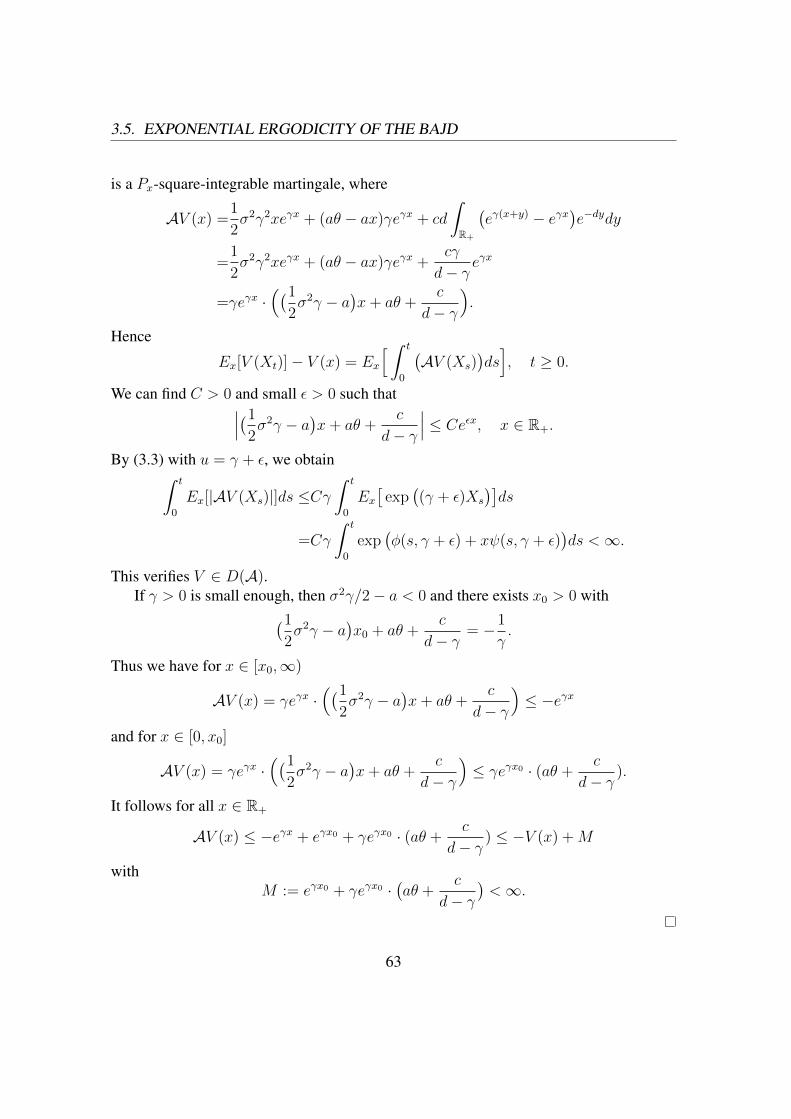
3.5. EXPONENTIAL ERGODICITY OF THE BAJD
is a Px-square-integrable martingale, where
AV (x) =1
2σ2γ2xeγx + (aθ − ax)γeγx + cd
∫R+
(eγ(x+y) − eγx
)e−dydy
=1
2σ2γ2xeγx + (aθ − ax)γeγx +
cγ
d− γeγx
=γeγx ·((1
2σ2γ − a
)x+ aθ +
c
d− γ
).
Hence
Ex[V (Xt)]− V (x) = Ex
[ ∫ t
0
(AV (Xs)
)ds], t ≥ 0.
We can find C > 0 and small ε > 0 such that∣∣∣(1
2σ2γ − a
)x+ aθ +
c
d− γ
∣∣∣ ≤ Ceεx, x ∈ R+.
By (3.3) with u = γ + ε, we obtain∫ t
0
Ex[|AV (Xs)|]ds ≤Cγ∫ t
0
Ex[
exp((γ + ε)Xs
)]ds
=Cγ
∫ t
0
exp(φ(s, γ + ε) + xψ(s, γ + ε)
)ds <∞.
This verifies V ∈ D(A).If γ > 0 is small enough, then σ2γ/2− a < 0 and there exists x0 > 0 with(1
2σ2γ − a
)x0 + aθ +
c
d− γ= −1
γ.
Thus we have for x ∈ [x0,∞)
AV (x) = γeγx ·((1
2σ2γ − a
)x+ aθ +
c
d− γ
)≤ −eγx
and for x ∈ [0, x0]
AV (x) = γeγx ·((1
2σ2γ − a
)x+ aθ +
c
d− γ
)≤ γeγx0 · (aθ +
c
d− γ).
It follows for all x ∈ R+
AV (x) ≤ −eγx + eγx0 + γeγx0 · (aθ +c
d− γ) ≤ −V (x) +M
withM := eγx0 + γeγx0 ·
(aθ +
c
d− γ)<∞.
63

3.5. EXPONENTIAL ERGODICITY OF THE BAJD
Lemma 9. Let the constants γ, k and M , as well as V (x) = exp(γx) be the same as inLemma 8. Then the BAJD satisfies
Ex[V (Xt)] ≤ e−ktV (x) +M
k,
or equivalently ∫R+
V (y)p(t, x, y)dy ≤ e−ktV (x) +M
k
for all x ∈ R+, t > 0.
Proof. Let V (x) = exp(γx) and g(x, t) := V (x) · exp(kt) = exp(γx + kt), wherethe constants γ and k are the same as in Lemma 8. Then gx = γ exp(γx + kt), gxx =γ2 exp(γx+ kt) and gt = k exp(γx+ kt). By applying Itô’s formula and then taking theexpectation, we get for all x ∈ R+, t > 0,
ektEx[V (Xt)]− V (x)
=Ex[g(Xt, t)]− Ex[g(X0, 0)]
=Ex
[ ∫ t
0
(eks · AV (Xs) + keks · V (Xs)
)ds]
≤Ex[ ∫ t
0
(eks ·
(− kV (Xs) +M
)+ keks · V (Xs)
)ds]
=Ex[ ∫ t
0
Meksds]
=M
kekt − M
k≤ M
kekt.
Thus for x ∈ R+, t > 0,
Ex[V (Xt)] ≤ e−ktV (x) +M
k.
Applying the main results of [46] and Lemma 9, we get the following theorem.
Theorem 10. Let h(x) := 1 + exp(γx) with the constant γ > 0 small enough. Then theBAJD is h-exponentially ergodic, namely there exist constants β ∈ (0, 1) and C ∈ (0,∞)such that
(3.51) ‖P t(x, ·)− π‖h ≤ C(eγx + 1
)βt, t > 0, x ∈ R+.
64

3.5. EXPONENTIAL ERGODICITY OF THE BAJD
Proof. Basically, we follow the proof of [46, Theorem 6.1]. Since the details of the proofmay obscure the idea, we now outline the reasoning behind our analysis. Instead of show-ing (3.51) for all t > 0, we first show (3.51) for some specially chosen tn > 0. Moreprecisely, we find constants β ∈ (0, 1) and C ∈ (0,∞) such that
(3.52) ‖P δn(x, ·)− π‖h ≤ C(eγx + 1
)βn, n ∈ Z+, x ∈ R+,
where δ > 0 is a constant and h := V + 1 = exp(γx) + 1. Then there is a simple trickin [46] to conclude (3.51) from (3.52). Thus, it suffices to show (3.52), or equivalently,to show the exponential ergodicity for the δ-skeleton chain of the BAJD. The exponentialergodicity of Markov chains has been studied in [44]. In particular, to show that a Markovchain is exponentially ergodic, [44, Theorem 6.3] provides some sufficient conditions: thechain admits a Foster-Lyapunov function and is irreducible and aperiodic, and all compactsubsets are petite. If we can show that these conditions are satisfied for the δ-skeletonchain of the BAJD, then we are done.
Now we proceed to show that the conditions of [44, Theorem 6.3] are satisfied for theδ-skeleton chain of X . For any δ > 0 we consider the δ-skeleton chain Y δ
n := Xnδ, n ∈Z+. Then (Y δ
n )n∈Z+ is a Markov chain with transition kernel p(δ, x, y) on the state spaceR+ and the law of the Yn (started from Y0 = x) is given by P δn(x, ·). It is easy to seethat invariant measures for the BAJD process (Xt)t≥0 are also invariant measures for(Y δ
n )n∈Z+ . Thus the probability measure π in Corollary 3 is also an invariant probabilitymeasure for the chain (Y δ
n )n∈Z+ .Let V (x) = exp(γx) be the same as in Lemma 9. It follows from the Markov property
and Lemma 9 that
Ex[V (Yn+1)|Y0, Y1, · · · , Yn] =
∫R+
V (y)p(δ, Yn, y)dy ≤ e−δkV (Yn) +M
k,
where k and M are positive constants. If we set V0 := V and Vn := V (Yn), n ∈ N, then
Ex[V1] ≤ e−δkV0(x) +M
k
andEx[Vn+1|Y0, Y1, · · · , Yn] ≤ e−δkVn +
M
k, n ∈ N.
Now we proceed to show that the chain (Y δn )n∈Z+ is λ-irreducible, strong aperiodic,
and all compact subsets of R+ are petite for the chain (Y δn )n∈Z+ .
“λ-irreducibility": We show that the Lebesgue measure λ on R+ is an irreducibilitymeasure for (Y δ
n )n∈Z+ . Let A ∈ B(R+) and λ(A) > 0, then
P [Y1 ∈ A|Y0 = x] = Px[Xδ ∈ A] =
∫A
p(δ, x, y)dy > 0,
65

3.5. EXPONENTIAL ERGODICITY OF THE BAJD
since p(δ, x, y) > 0 for any x ∈ R+ and y > 0. This shows that the chain (Y δn )n∈Z+ is
irreducible with λ being an irreducibility measure.“Strong aperiodicity" (see [44, p.561] for a definition): To show the strong aperiodicity
of (Yn)n∈N0 , we need to find a set C ∈ B(R+), a probability measure ν with ν(C) = 1,and ε > 0 such that
(3.53) L(x,C) > 0, x ∈ R+
and
(3.54) Px(Y1 ∈ A) ≥ ε · ν(A), x ∈ C, A ∈ B(R+),
where L(x,C) := Px(Ym ∈ C for some m ∈ N). To this end set C := [0, 1] and g(y) :=infx∈[0,1] p(δ, x, y), y > 0. Since for fixed y > 0 the function p(δ, x, y) is strictly positiveand continuous in x ∈ [0, 1], thus we have g(y) > 0 and 0 <
∫(0,1]
g(y)dy ≤ 1. Define
ν(A) :=1∫
(0,1]g(y)dy
∫A∩(0,1]
g(y)dy, A ∈ B(R+).
Then for any x ∈ [0, 1] and A ∈ B(R+) we get
Px(Y1 ∈ A) =
∫A
p(δ, x, y)dy ≥∫A∩(0,1]
g(y)dy = ν(A)
∫(0,1]
g(y)dy,
so (3.54) holds with ε :=∫
(0,1]g(y)dy.
Obviously
L(x, [0, 1]) ≥ Px(Y1 ∈ [0, 1]) = Px(Xδ ∈ [0, 1]) =
∫[0,1]
p(δ, x, y)dy > 0
for all x ∈ R+, which verifies (3.53).“Compact subsets are petite": We have shown that λ is an irreducibility measure for
(Y δn )n∈Z+ . According to [44, Theorem 3.4(ii)], to show that all compact sets are petite,
it suffices to prove the Feller property of (Y δn )n∈Z+ , but this follows from the fact that
(Y δn )n∈Z+ is a skeleton chain of the BAJD process (Xt)t≥0, which possesses the Feller
property.According to [44, Theorem 6.3] (see also the proof of [44, Theorem 6.1]), the proba-
bility measure π is the only invariant probability measure of the chain (Y δn )n∈Z+ and there
exist constants β ∈ (0, 1) and C ∈ (0,∞) such that
‖P δn(x, ·)− π‖h ≤ C(eγx + 1
)βn, n ∈ Z+, x ∈ R+,
where h := V + 1 = exp(γx) + 1.Then we can proceed as in [46, p.536] and get the inequality (3.51).
66

3.6. CALIBRATION FOR THE BAJD-PROCESS
Since ‖µ‖TV ≤ ‖µ‖h, it follows immediately the following corollary.
Corollary 5. The BAJD is exponentially ergodic, namely there exist constants β ∈ (0,∞)and C ∈ (0,∞) such that
(3.55) ‖P t(x, ·)− π‖TV ≤ C(eγx + 1
)βt, ∀t > 0, x ∈ R+.
Remark 11. In Chapter 2 we proved that the CIR process is positive Harris recurrent. If weallow the parameter c = 0, then all results of this section still hold and thus are also truefor the CIR process. In particular Theorem 10 is also true for the CIR process. In this casethe unique invariant probability measure of the CIR process is the Gamma distributionΓ(2aθ/σ2, σ2/(2a)
)and has the characteristic function
(1− σ2u/(2a)
)−2aθ/σ2
.
3.6 Calibration for the BAJD-processNow, we will use the results of this chapter to provide another consequence of Harris
recurrence property for the BAJD process. We have already shown in section (3.4) thatour result on the positive Harris recurrence of the BAJD provides another way of provingthe existence and uniqueness of an invariant probability measure for the BAJD. We denoteit by π, this measure is the convolution of a Gamma distribution with Bessel or mixtureof Bessel distributions.
From the ergodicity point of view, we also show in corollary (4) that another con-sequence of the positive Harris recurrence is the limit theorem for additive function-als, namely we show that for all f ∈ B(R+), 1
t
∫ t0f(Xs)ds converges almost surely to∫
R+f(x)π(dx). Obviously the BAJD process is strongly ergodic. In fact, it follow from
the exponential ergodicity result of the BAJD, which was proved in the last section. Notethat, the exponential ergodicity implies strong ergodicity but not vice-versa. Also, strongergodicity of the BAJD follow from [29, Theorem 20.12], which say that any Harris re-current Feller process is strongly ergodic.
Let us first recall the definition of affine term structure (see e.g. [13, Definition 3.1]).
Definition 12. An R+−valued homogeneous Markov process X with
(3.56) Ex[e−
∫ t0 Xsds
]= ep(t)+xq(t)
for some functions p and q, is said to provide an affine term structure (ATS).
We want the term e−∫ t0 Xsds to be well-defined R+−valued adapted process, for each
Px. This is equivalent to assume that the process X is progressively measurable and∫ t
0
Xsds <∞, Px − a.s. ∀t, x ∈ R+.
67
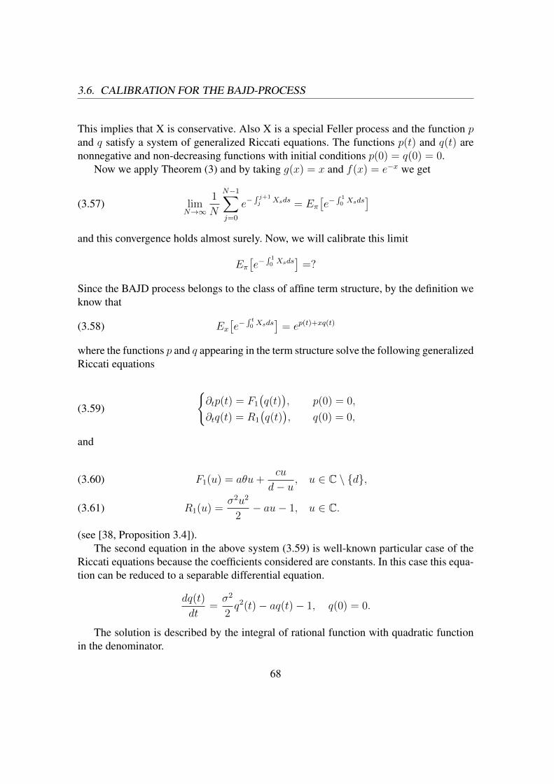
3.6. CALIBRATION FOR THE BAJD-PROCESS
This implies that X is conservative. Also X is a special Feller process and the function pand q satisfy a system of generalized Riccati equations. The functions p(t) and q(t) arenonnegative and non-decreasing functions with initial conditions p(0) = q(0) = 0.
Now we apply Theorem (3) and by taking g(x) = x and f(x) = e−x we get
(3.57) limN→∞
1
N
N−1∑j=0
e−∫ j+1j Xsds = Eπ
[e−
∫ 10 Xsds
]and this convergence holds almost surely. Now, we will calibrate this limit
Eπ[e−
∫ 10 Xsds
]=?
Since the BAJD process belongs to the class of affine term structure, by the definition weknow that
(3.58) Ex[e−
∫ t0 Xsds
]= ep(t)+xq(t)
where the functions p and q appearing in the term structure solve the following generalizedRiccati equations
(3.59)
∂tp(t) = F1
(q(t)
), p(0) = 0,
∂tq(t) = R1
(q(t)
), q(0) = 0,
and
F1(u) = aθu+cu
d− u, u ∈ C \ d,(3.60)
R1(u) =σ2u2
2− au− 1, u ∈ C.(3.61)
(see [38, Proposition 3.4]).The second equation in the above system (3.59) is well-known particular case of the
Riccati equations because the coefficients considered are constants. In this case this equa-tion can be reduced to a separable differential equation.
dq(t)
dt=σ2
2q2(t)− aq(t)− 1, q(0) = 0.
The solution is described by the integral of rational function with quadratic functionin the denominator.
68

3.6. CALIBRATION FOR THE BAJD-PROCESS
∫ t
0
dq(s)σ2
2q2(s)− aq(s)− 1
=
∫ t
0
ds = t.
Now∫ t
0
dq(s)σ2
2q2(s)− aq(s)− 1
=
∫ t
0
( 1
q(s)− a−√a2+2σ2
σ2
+−1
q(s)− a+√a2+2σ2
σ2
)dq(s)
= −√a2 + 2σ2t.
Finally one can get
q(t) =1− eb1t
c1 + d1eb1t
where c1 = −a+√a2+2σ2
2, d1 = a−
√a2+2σ2
2and b1 = −
√a2 + 2σ2. Now for the first
equation of the system (3.59), we denote
I1 := aθ
∫ t
0
q(s)ds = aθ
∫ t
0
1− eb1s
c1 + d1eb1sds
and
I2 := c
∫ t
0
q(s)
d− q(s)ds = c
∫ t
0
1− eb1s
(dd1 + 1)eb1s + (dc1 − 1)ds
By change of variable r = eb1s in I10it follow that
I1 =2aθ
σ2log( b1e
d1t
c1 + d1eb1t)
=2aθ
σ2log(b1e
(a+b1)t/2
c1 + d1eb1t)
For the second integral I2, we distinguish between two cases. If d 6= d1 then by change ofvariable is easy to get
I2 =ct
c1d− 1− cd
12σ2d2 − ad− 1
log((1 + dd1)eb1t + c1d− 1
b1d
).
If d = d1 then we get
I2 =ct
c1d− 1− cd
12σ2d2 − ad− 1
+d1
b21
(eb1t − 1
)Therefore the solution p can be represented explicitly in the following way:
p(t) =
2aθσ2 log
(b1e(a+b1)t/2
c1+d1eb1t
)+ ct
c1d−1
− cd12σ2d2−ad−1
log(
(1+dd1)eb1t+c1d−1b1d
), if d 6= d1,
2aθσ2 log
(b1e(a+b1)t/2
c1+d1eb1t
)+ ct
c1d−1+ d1
b21
(eb1t − 1
),
if d = d1.
69

3.6. CALIBRATION FOR THE BAJD-PROCESS
Since the BAJD has an explicit form of invariant measure hence we calibrate this limit inthe explicit form
Eπ[e−
∫ 10 Xsds
]=
∫ ∞0
Ex[e−
∫ 10 Xsds
]π(dx)
=
∫ ∞0
ep(1)+xq(1)π(dx)
= ep(1)
∫ ∞0
exq(1)π(dx)
=
ep(1)(1− σ2
2aq(1)
)− 2aθσ2 ·
(d−σ
2dq(1)2a
d−q(1)
) c
a−σ2d2 , if ∆ 6= 0,
ep(1)(1− σ2
2aq(1)
)− 2aθσ2 · exp
(cq(1)
a(d−q(1))
), if ∆ = 0.
where ∆ = a− σ2d2
.
70
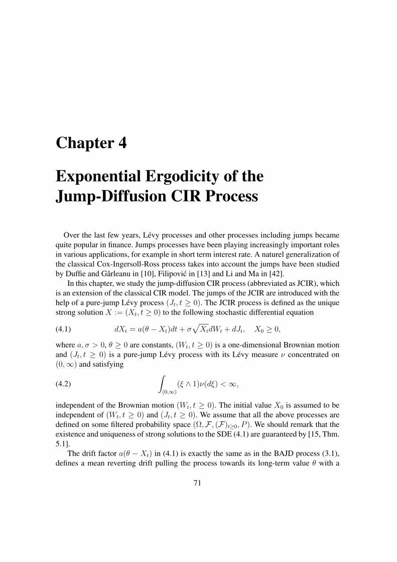
Chapter 4
Exponential Ergodicity of theJump-Diffusion CIR Process
Over the last few years, Lévy processes and other processes including jumps becamequite popular in finance. Jumps processes have been playing increasingly important rolesin various applications, for example in short term interest rate. A naturel generalization ofthe classical Cox-Ingersoll-Ross process takes into account the jumps have been studiedby Duffie and Gârleanu in [10], Filipovic in [13] and Li and Ma in [42].
In this chapter, we study the jump-diffusion CIR process (abbreviated as JCIR), whichis an extension of the classical CIR model. The jumps of the JCIR are introduced with thehelp of a pure-jump Lévy process (Jt, t ≥ 0). The JCIR process is defined as the uniquestrong solution X := (Xt, t ≥ 0) to the following stochastic differential equation
(4.1) dXt = a(θ −Xt)dt+ σ√XtdWt + dJt, X0 ≥ 0,
where a, σ > 0, θ ≥ 0 are constants, (Wt, t ≥ 0) is a one-dimensional Brownian motionand (Jt, t ≥ 0) is a pure-jump Lévy process with its Lévy measure ν concentrated on(0,∞) and satisfying
(4.2)∫
(0,∞)
(ξ ∧ 1)ν(dξ) <∞,
independent of the Brownian motion (Wt, t ≥ 0). The initial value X0 is assumed to beindependent of (Wt, t ≥ 0) and (Jt, t ≥ 0). We assume that all the above processes aredefined on some filtered probability space (Ω,F , (F)t≥0, P ). We should remark that theexistence and uniqueness of strong solutions to the SDE (4.1) are guaranteed by [15, Thm.5.1].
The drift factor a(θ − Xt) in (4.1) is exactly the same as in the BAJD process (3.1),defines a mean reverting drift pulling the process towards its long-term value θ with a
71

4.1. CHARACTERISTIC FUNCTION OF THE JCIR
speed of adjustment equal to a. Since the diffusion coefficient σ√Xt in the SDE (4.1) is
degenerate at 0 and only positive jumps are allowed, the JCIR process (Xt, t ≥ 0) staysnon-negative if X0 ≥ 0. This fact can be shown rigorously with the help of comparisontheorems for SDEs, for more details we refer the readers to [15].
In this chapter we are interested in two problems concerning the JCIR defined in(4.1). The first one is to study the transition density estimates of the JCIR, namely wefind a lower bound on the transition densities of the JCIR. Our idea to establish the lowerbound of the transition densities is as follows. It well known that the JCIR is also anaffine processes in R+. Based on the exponential-affine structure of the JCIR, we are ableto compute its characteristic function explicitly. Moreover, this enables us to representthe distribution of the JCIR as the convolution of two distributions. The first distributioncoincides with the distribution of the CIR model. However, the second distribution ismore complicated. We will give a sufficient condition such that the second distributionis singular at the point 0. In this way we derive a lower bound estimate of the transitiondensities of the JCIR.
4.1 Characteristic function of the JCIRIn this section we use the exponential-affine structure of the JCIR process to derive itscharacteristic functions.
We recall that the JCIR process (Xt, t ≥ 0) is defined to be the solution to (4.1) andit depends obviously on its initial value X0. From now on we denote by (Xx
t , t ≥ 0) theJCIR process started from an initial point x ≥ 0, namely
(4.3) dXxt = a(θ −Xx
t )dt+ σ√Xxt dWt + dJt, Xx
0 = x.
Since the JCIR process is an affine jump diffusion, the corresponding characteristicfunctions of (Xx
t , t ≥ 0) is of an exponential-affine form, i.e. there exist functions φ(t, u)and ψ(t, u) such that
(4.4) E[euX
xt]
= eφ(t,u)+xψ(t,u), for all t ≥ 0, u ∈ U , x ≥ 0,
where U := u ∈ C : <u ≤ 0, <u denotes the real part of u. Moreover, the functionsφ(t, u) and ψ(t, u) are the unique solutions of the generalized Riccati equations
(4.5)
∂tφ(t, u) = F
(ψ(t, u)
), φ(0, u) = 0,
∂tψ(t, u) = R(ψ(t, u)
)ψ(0, u) = u ∈ U ,
72

4.1. CHARACTERISTIC FUNCTION OF THE JCIR
with the functions F and R are of Lévy-Khitchine form
F (u) = aθu+
∫(0,∞)
(euξ − 1)ν(dξ),(4.6)
R(u) =σ2u2
2− au.(4.7)
For general case see [[13], Theorem 4.3].Note that, it is not difficult to find the explicit form of the functions ∂tφ and ∂tψ. We
have to proceed as in the Section (2.1). More precisely, we can find the functions ∂tφ and∂tψ under the initial conditions such that
Mt := exp(φ(T − t, u) +Xtψ(T − t, u)
)is a martingale. We can derive the generalized Riccati equation by applying Itô formulafor the jumps diffusion and then we collect the coefficients.
Solving the system (4.5) gives φ(t, u) and ψ(t, u) in their explicit forms. One canremark that the second equation of the generalized Riccati equations is a Bernoulli differ-ential equation with n = 2. Therefore the solution ψ can be represented explicitly in thefollowing way:
ψ(t, u) = ψ(0, u)e−∫ t0 ads
(1− u
∫ t
0
σ2
2e−asds
)−1
=ue−at
1− σ2
2au(1− e−at)
.(4.8)
Note that the first Riccati equation is just an integral, and φ may be written explicitly as:
φ(t, u) =−2aθ
σ2
∫ t
0
σ2
2ue−as
1− σ2
2au(1− e−as)
ds+
∫ t
0
∫(0,∞)
(eξψ(s,u) − 1
)ν(dξ)ds
(4.9) = −2aθ
σ2log(1− σ2
2au(1− e−at)
)+
∫ t
0
∫(0,∞)
(eξψ(s,u) − 1
)ν(dξ)ds.
Here the complex-valued logarithmic function log(·) is understood to be its main branchdefined on C \ 0.It follows from (4.4), (4.8) and (4.9) that the characteristic functions of (Xx
t , t ≥ 0) isgiven by
(4.10) E[euXxt ] = ϕ1(t, u, x)ϕ2(t, u), u ∈ U ,
73

4.1. CHARACTERISTIC FUNCTION OF THE JCIR
where ϕ1(t, u, x) and ϕ2(t, u) are defined as follows, for t ≥ 0 and u ∈ U
ϕ1(t, u, x) : =(1− σ2
2au(1− e−at)
)− 2aθσ2 exp
( xue−at
1− σ2
2au(1− e−at)
),
ϕ2(t, u) : = exp(∫ t
0
∫ ∞0
(eξψ(s,u) − 1
)ν(dξ)ds
),(4.11)
where the complex-valued power function z−2aθ/σ2:= exp
(− (2aθ/σ2) log z
)is also
understood to be its main branch defined on C \ 0.According to the parameters of the JCIR process we look at two special cases:
4.1.1 Special Case i): ν = 0, No JumpsNotice that the case ν = 0 corresponds to the classical CIR model (Yt, t ≥ 0) satisfyingthe following stochastic differential equation
(4.12) dY xt = a(θ − Y x
t )dt+ σ√Y xt dWt, Y x
0 = x ≥ 0.
It follows from (4.10) that the characteristic function of (Y xt , t ≥ 0) coincides with
ϕ1(t, u, x), namely, for u ∈ U
E[euYxt ] = ϕ1(t, u, x).
It is well known that the classical CIR model (Y xt , t ≥ 0) has transition density functions
f(t, x, y) given by
(4.13) f(t, x, y) = κe−u−v(vu
) q2Iq(2(uv)
12
)for t > 0, x > 0 and y ≥ 0, where
κ ≡ 2a
σ2(
1− e−at) , u ≡ κxe−at,
v ≡ κy, q ≡ 2aθ
σ2− 1,
and Iq(·) is the modified Bessel function of the first kind of order q. For x = 0 the formulaof the density function f(t, x, y) is given by
(4.14) f(t, 0, y) =c
Γ(q + 1)vqe−v
for t > 0 and y ≥ 0.
74

4.2. LOWER BOUND FOR THE TRANSITION DENSITIES OF JCIR
4.1.2 Special Case ii): θ = 0 and x = 0
We denote by (Zt, t ≥ 0) the JCIR process given by
(4.15) dZt = −aZtdt+ σ√ZtdWt + dJt, Z0 = 0.
In this particular case the characteristic functions of (Zt, t ≥ 0) is equal to ϕ2(t, u),namely, for u ∈ U
(4.16) E[euZt ] = ϕ2(t, u).
One can notice that ϕ2(t, u) resembles the characteristic function of a compound Poissondistribution.
4.2 Lower bound for the transition densities of JCIRIn this section we will find some conditions on the Lévy measure ν of (Jt, t ≥ 0) suchthat an explicit lower bound for the transition densities of the JCIR process given in (4.3)can be derived. As a first step we show that the law of Xx
t , t > 0, in (4.3) is absolutelycontinuous with respect to the Lebesgue measure and thus possesses a density function.
Lemma 10. Consider the JCIR process (Xxt , t ≥ 0) (started from x ≥ 0) that is defined
in (4.3). Then for any t > 0 and x ≥ 0 the law ofXxt is absolutely continuous with respect
to the Lebesgue measure and thus possesses a density function p(t, x, y), y ≥ 0.
Proof. As shown in the previous section, it holds
E[euXxt ] = ϕ1(t, u, x)ϕ2(t, u) = E[euY
xt ]E[euZt ],
therefore the law of Xxt , denoted by µXx
t, is the convolution of the laws of µY xt and µZt .
Where µY xt and µZt are the laws of Y xt and Zt respectively. Since (Y x
t , t ≥ 0) is the well-known classical CIR process and has transition density function f(t, x, y), t > 0, x, y ≥ 0with respect to the Lebesgue measure, thus µXx
tis also absolutely continuous with respect
to the Lebesgue measure and possesses a density function.
In order to get a lower bound for the transition densities of the JCIR process we needthe following lemma.
Lemma 11. Suppose that∫
(0,1)ξ ln(1/ξ)ν(dξ) < ∞. Then ϕ2 defined by (4.11) is the
characteristic function of a compound Poisson distribution. In particular, P (Zt = 0) > 0for all t > 0, where (Zt, t ≥ 0) is defined by (4.15).
75

4.2. LOWER BOUND FOR THE TRANSITION DENSITIES OF JCIR
Proof. It follows from (4.8), (4.11) and (4.16) that
E[euZt ] = ϕ2(t, u) = exp
(∫ t
0
∫(0,∞)
(exp
(ξue−as
1−(σ2/2a)(1−e−as)u
)− 1)ν(dξ)ds
),
where u ∈ U . Define
∆ :=
∫ t
0
∫(0,∞)
(exp
( ξue−as
1− (σ2/2a)(1− e−as)u
)− 1)ν(dξ)ds.
If we rewrite
(4.17) exp( ξe−asu
1− (σ2/2a)(1− e−as)u
)= exp
( αu
β − u
),
where
(4.18)
α :=
2aξ
σ2(eas − 1)> 0,
β :=2aeas
σ2(eas − 1)> 0,
then we recognize that the right-hand side of (4.17) is the characteristic function ofa Bessel distribution with parameters α and β. Recall that a probability measure µα,β on(R+,B(R+)
)is called a Bessel distribution with parameters α and β if
(4.19) µα,β(dx) = e−αδ0(dx) + βe−α−βx√
α
βxI1(2
√αβx)dx,
where δ0 is the Dirac measure at the origin and I1 is the modified Bessel function of thefirst kind, namely,
I1(r) =r
2
∞∑k=0
(14r2)k
k!(k + 1)!, r ∈ R.
For more properties of Bessel distributions we refer the readers to [19, Sect. 3] (see also[12, p.438] and [27, Sect. 3]). Let µα,β denote the characteristic function of the Besseldistribution µα,β with parameters α and β which are defined in (4.18). It follows from[27, Lemma 3.1] that
µα,β(u) = exp( αu
β − u
)= exp
( ξe−asu
1− (σ2/2a)(1− e−as)u
).
76

4.2. LOWER BOUND FOR THE TRANSITION DENSITIES OF JCIR
Therefore
∆ =
∫ t
0
∫(0,∞)
(µα,β(u)− 1
)ν(dξ)ds
=
∫ t
0
∫(0,∞)
(eαuβ−u − e−α + e−α − 1
)ν(dξ)ds.
Set
λ :=
∫ t
0
∫(0,∞)
(1− e−α
)ν(dξ)ds
=
∫ t
0
∫(0,∞)
(1− e−
2aξ
σ2(eas−1)
)ν(dξ)ds.(4.20)
If λ <∞, then
∆ =
∫ t
0
∫(0,∞)
(eαuβ−u − e−α
)ν(dξ)ds− λ
= λ(1
λ
∫ t
0
∫(0,∞)
(eαuβ−u − e−α
)ν(dξ)ds− 1
).
The fact that λ <∞ will be shown later in this proof.Next we show that the term (1/λ)
∫ t0
∫(0,∞)
(exp
(αu/(β − u)
)− exp(−α)
)ν(dξ)ds can
be viewed as the characteristic function of a probability measure ρ. To define ρ, we firstconstruct the following measures
mα,β(dx) := βe−α−βx√
α
βxI1(2
√αβx)dx, x ≥ 0,
where I1 is the modified Bessel function of the first kind. Noticing that the measure mα,β
is the absolute continuous component of the measure µα,β in (4.19), we easily get
mα,β(u) = µα,β(u)− e−α = eαuβ−u − e−α,
where mα,β(u) :=∫∞
0euxmα,β(dx) for u ∈ U . Recall that the parameters α and β defined
by (4.18) depend on the variables ξ and s. We can define a measure ρ on R+ as follows:
ρ :=1
λ
∫ t
0
∫(0,∞)
mα,β ν(dξ)ds.
77

4.2. LOWER BOUND FOR THE TRANSITION DENSITIES OF JCIR
By the definition of the constant λ in (4.20) we get
ρ(R+) =1
λ
∫ t
0
∫(0,∞)
mα,β(R+)ν(dξ)ds
=1
λ
∫ t
0
∫(0,∞)
(1− e−α)ν(dξ)ds
= 1,
i.e. ρ is a probability measure on R+, and for u ∈ U
ρ(u) =
∫(0,∞)
euxρ(dx)
=1
λ
∫ t
0
∫(0,∞)
(eαuβ−u − e−α)ν(dξ)ds.
Thus ∆ = λ(ρ(u)− 1) and E[euZt ] = ϕ2(t, u) = eλ(ρ(u)−1) is the characteristic functionof a compound Poisson distribution.Now we verify that λ <∞. Noticing that
λ =
∫ t
0
∫(0,∞)
(1− e−α
)ν(dξ)ds
=
∫ t
0
∫(0,∞)
(1− e−
2aξ
σ2(eas−1)
)ν(dξ)ds
=
∫(0,∞)
∫ t
0
(1− e−
2aξ
σ2(eas−1)
)dsν(dξ),
we introduce the change of variables2aξ
σ2(eas − 1):= y and then get
dy = − 2aξ
σ2(eas − 1)2aeasds
= −y2σ2
2ξ
(2aξ
σ2y+ 1)ds.
Therefore
λ =
∫(0,∞)
ν(dξ)
∫ 2aξ
σ2(eat−1)
∞(1− e−y) −2ξ
2aξy + σ2y2dy
=
∫(0,∞)
ν(dξ)
∫ ∞2aξ
σ2(eat−1)
(1− e−y) 2ξ
2aξy + σ2y2dy
=
∫(0,∞)
ν(dξ)
∫ ∞ξδ
(1− e−y) 2ξ
2aξy + σ2y2dy,
78

4.2. LOWER BOUND FOR THE TRANSITION DENSITIES OF JCIR
where δ :=σ2(eat − 1)
2a. Define
M(ξ) :=
∫ ∞ξδ
(1− e−y) 2ξ
2aξy + σ2y2dy.
Then M(ξ) is continuous on (0,∞). As ξ → 0 we get
M(ξ) =
∫ 1
ξδ
(1− e−y) 2ξ
2aξy + σ2y2dy + 2ξ
∫ ∞1
(1− e−y) dy
2aξy + σ2y2
≤ 2ξ
∫ 1
ξδ
y
2aξy + σ2y2dy + 2ξ
∫ ∞1
1
2aξy + σ2y2dy
≤ 2ξ
∫ 1
ξδ
1
2aξ + σ2ydy + 2ξ
∫ ∞1
1
σ2y2dy.
Since
2ξ
∫ 1
ξδ
1
2aξ + σ2ydy =
2ξ
σ2
[ln(2aξ + σ2y)
]1
ξδ
=2ξ
σ2ln(2aξ + σ2)− 2ξ
σ2ln(2aξ +
σ2ξ
δ)
≤ c1ξ + c2ξ ln(1
ξ) ≤ c3ξ ln(
1
ξ)
for sufficiently small ξ, we conclude that
M(ξ) ≤ c4ξ ln(1
ξ), as ξ → 0.
If ξ →∞, then
M(ξ) ≤∫ ∞ξδ
(1− e−y) 2ξ
2aξy + σ2y2dy
≤∫ ∞ξδ
2ξ
2aξy + σ2y2dy ≤ 2ξ
∫ ∞ξδ
1
σ2y2dy
=2ξ
σ2
∫ ∞ξδ
d(−1
y) =
2ξ
σ2
[− 1
y
]∞ξδ
=2ξ
σ2
δ
ξ=
2δ
σ2:= c5 <∞.
79

4.2. LOWER BOUND FOR THE TRANSITION DENSITIES OF JCIR
Therefore,
λ ≤ c4
∫ 1
0
ξ ln(1
ξ)ν(dξ) + c5
∫ ∞1
1ν(dξ) <∞.
With the help of the above Lemma 11 we can easily prove the following proposition.
Proposition 3. Let p(t, x, y), t > 0, x, y ≥ 0 denote the transition density of the JCIRprocess (Xx
t , t ≥ 0) defined in (4.3). Suppose that∫
(0,1)ξ ln(1
ξ)ν(dξ) < ∞. Then for all
t > 0, x, y ≥ 0 we have
p(t, x, y) ≥ P (Zt = 0)f(t, x, y),
where P (Zt = 0) > 0 for all t > 0 and f(t, x, y) are transition densities of the classicalCIR process.
Proof. According to Lemma 11, we have P (Zt = 0) > 0 for all t > 0. Since
E[euXxt ] = ϕ1(t, u, x)ϕ2(t, u) = E[euY
xt ]E[euZt ],
the law of Xxt , denoted by µXx
t, is the convolution of the laws of µY xt and µZt . Where µY xt
and µZt are the laws of Y xt and Zt respectively. Thus for all A ∈ B(R+)
µXxt(A) =
∫R+
µY xt (A− y)µZt(dy)
≥∫0µY xt (A− y)µZt(dy)
≥ µY xt (A)µZt(0)≥ P (Zt = 0)µY xt (A)
≥ P (Zt = 0)
∫A
f(t, x, y)dy,
where A − y = z − y, z ∈ A and f(t, x, y) are the transition densities of the classicalCIR process given in (4.13). Since A ∈ B(R+) is arbitrary, we get
p(t, x, y) ≥ P (Zt = 0)f(t, x, y)
for all t > 0, x, y ≥ 0.
80

4.3. EXPONENTIAL ERGODICITY OF JCIR
4.3 Exponential ergodicity of JCIRNow we consider the second problem of this chapter which is the exponential ergodic-ity of the JCIR. According to the main results of [32] (see also [38]), the JCIR has aunique invariant probability measure π, given that some integrability condition on theLévy measure of (Jt, t ≥ 0) is satisfied. Under some sharper assumptions we show thatthe convergence of the law of the JCIR process to its invariant probability measure underthe total variation norm is exponentially fast, which is called the exponential ergodicity.Our method is the same as in Chapter 3 Section (3.5), namely we show the existence of aFoster-Lyapunov function and then apply the general framework of [44, 45, 46] to get theexponential ergodicity.
In this section we find some sufficient conditions such that the JCIR process is expo-nentially ergodic. We have derived a lower bound for the transition densities of the JCIRprocess in the previous section. Next we show that the function V (x) = x, x ≥ 0, is aFoster-Lyapunov function for the JCIR process.
Lemma 12. Suppose that∫
(1,∞)ξν(dξ) < ∞. Then the function V (x) = x, x ≥ 0, is a
Foster-Lyapunov function for the JCIR process defined in (4.3), in the sense that for allt > 0, x ≥ 0,
E[V (Xxt )] ≤ e−atV (x) +M,
where 0 < M <∞ is a constant.
Proof. We know that µXxt
= µY xt ∗ µZt , therefore
E[Xxt ] = E[Y x
t ] + E[Zt].
Since (Y xt , t ≥ 0) is the classical CIR process starting from x, it is known that µY xt is a
non-central Chi-squared distribution and thus E[Y xt ] < ∞. Next we show that E[Zt] <
∞.Let u ∈ (−∞, 0). By using Fatou’s Lemma we get
E[Zt] = E[limu→0
euZt − 1
u
]≤ lim inf
u→0E[euZt − 1
u
]= lim inf
u→0
E[euZt ]− 1
u.
Recall that
E[euZt ] = ϕ2(t, u) = exp(∫ t
0
∫(0,∞)
(e
ξue−as
1−(σ2/2a)(1−e−as)u − 1)ν(dξ)ds
)= e∆(u).
81

4.3. EXPONENTIAL ERGODICITY OF JCIR
Then we have for all u ≤ 0
∂
∂u
(exp
( ξue−as
1− (σ2/2a)(1− e−as)u
)− 1
)=
ξe−as(1− (σ2/2a)(1− e−as)u
)2 exp( ξue−as
1− (σ2/2a)(1− e−as)u
)≤ ξe−as(
1− (σ2/2a)(1− e−as)u)2 ≤ ξe−as
and further ∫ t
0
∫(0,∞)
ξe−asν(dξ)ds <∞.
Thus ∆(u) is differentiable in u and
∆′(0) =
∫ t
0
∫(0,∞)
ξe−asν(dξ)ds =1− e−at
a
∫(0,∞)
ξν(dξ).
It follows that
E[Zt] ≤ lim infu→0
ϕ2(t, u)− ϕ2(t, 0)
u
=∂ϕ2(t, u)
∂u
∣∣∣u=0
= e∆(0)∆′(0)
=1− e−at
a
∫(0,∞)
ξν(dξ).
Therefore under the assumption∫
(0,∞)
ξν(dξ) <∞ we have proved that E[Zt] < ∞.
Furthermore,
E[Zt] =∂
∂u
(E[euZt ]
)∣∣∣u=0
=1− e−at
a
∫(0,∞)
ξν(dξ).
On the other hand,
E[euYxt ] =
(1− (σ2/2a)u(1− e−at)
)−2aθ/σ2
exp( xue−at
1− (σ2/2a)u(1− e−at)
).
With a similar argument as above we get
E[Y xt ] =
∂
∂u
(E[euY
xt ])∣∣∣
u=0= θ(1− e−at) + xe−at.
82

4.3. EXPONENTIAL ERGODICITY OF JCIR
Altogether we get
E[Xxt ] = E[Y x
t ] + E[Zt]
= (1− e−at)(θ +
1− e−at
a
)+ xe−at
≤ θ +1
a+ xe−at,
namely
E[V (Xxt )] ≤ θ +
1
a+ e−atV (x).
If∫
(1,∞)ξν(dξ) <∞, then there exists a unique invariant probability measure for the
JCIR process. This fact follows from [38, Thm. 3.16] and [32, Prop. 3.1]. Let ‖ · ‖TVdenote the total-variation norm for signed measures on R+, namely
‖µ‖TV = supA∈B(R+)
|µ(A)|.
Let P t(x, ·) := P (Xxt ∈ ·) be the distribution of the JCIR process at time t started
from the initial point x ≥ 0. Now we prove the main result of this chapter.
Theorem 12. Assume that∫(1,∞)
ξ ν(dξ) <∞ and∫
(0,1)
ξ ln(1
ξ)ν(dξ) <∞.
Let π be the unique invariant probability measure for the JCIR process. Then the JCIRprocess is exponentially ergodic, namely there exist constants 0 < β < 1 and 0 < B <∞such that
(4.21) ‖P t(x, ·)− π‖TV ≤ B(x+ 1
)βt, t ≥ 0, x ∈ R+.
Proof. Basically, we follow the proof of [46, Thm. 6.1]. For any δ > 0 we consider the δ-skeleton chain ηxn := Xx
nδ, n ∈ Z+, where Z+ denotes the set of all non-negative integers.Then (ηxn)n∈Z+ is a Markov chain on the state space R+ with transition kernel P δ(x, ·) andstarting point ηx0 = x. It is easy to see that the measure π is also an invariant probabilitymeasure for the chain (ηxn)n∈Z+ , x ≥ 0.
Let V (x) = x, x ≥ 0. It follows from the Markov property and Lemma 12 that
E[V (ηxn+1)|ηx0 , ηx1 , · · · , ηxn] =
∫R+
V (y)P δ(ηxn, dy) ≤ e−aδV (ηxn) +M,
83

4.3. EXPONENTIAL ERGODICITY OF JCIR
where M is a positive constant. If we set V0 := V and Vn := V (ηxn), n ∈ N, then
E[V1] ≤ e−aδV0(x) +M
andE[Vn+1|ηx0 , ηx1 , · · · , ηxn] ≤ e−aδVn +M, n ∈ N.
Now we proceed to show that the chain (ηxn)n∈Z+ , x ≥ 0, is λ-irreducible, strongaperiodic, and all compact subsets of R+ are petite for the chain (ηxn)n∈Z+ .
“λ-irreducibility": We show that the Lebesgue measure λ on R+ is an irreducibilitymeasure for (ηxn)n∈Z+ . Let A ∈ B(R+) and λ(A) > 0. Then it follows from Prop. 3 that
P [ηx1 ∈ A|ηx0 = x] = P (Xxδ ∈ A) ≥ P (Zδ = 0)
∫A
f(δ, x, y)dy > 0,
since f(δ, x, y) > 0 for any x ∈ R+ and y > 0. This shows that the chain (ηxn)n∈Z+ isirreducible with λ being an irreducibility measure.
“Strong aperiodicity" (see [44, p.561] for a definition): To show the strong aperiodicityof (ηxn)n∈Z0 , we need to find a set B ∈ B(R+), a probability measure m with m(B) = 1,and ε > 0 such that
(4.22) L(x,B) > 0, x ∈ R+,
and
(4.23) P (ηx1 ∈ A) ≥ εm(A), x ∈ C, A ∈ B(R+),
where L(x,B) := P (ηxn ∈ B for some n ∈ N). To this end set B := [0, 1] and g(y) :=infx∈[0,1] f(δ, x, y), y > 0. Since for fixed y > 0 the function f(δ, x, y) strictly positiveand continuous in x ∈ [0, 1], thus we have g(y) > 0 and 0 <
∫(0,1]
g(y)dy ≤ 1. Define
m(A) :=1∫
(0,1]g(y)dy
∫A∩(0,1]
g(y)dy, A ∈ B(R+).
Then for any x ∈ [0, 1] and A ∈ B(R+) we get
P (ηx1 ∈ A) = P (Xxδ ∈ A)
≥ P (Zδ = 0)
∫A
f(δ, x, y)dy
≥ P (Zδ = 0)
∫A∩(0,1]
g(y)dy
≥ P (Zδ = 0)m(A)
∫(0,1]
g(y)dy,
84

4.3. EXPONENTIAL ERGODICITY OF JCIR
so (4.23) holds with ε := P (Zδ = 0)∫
(0,1]g(y)dy.
Obviously
L(x, [0, 1]) ≥ P (ηx1 ∈ [0, 1]) = P (Xxδ ∈ [0, 1]) ≥ P (Zδ = 0)
∫[0,1]
f(δ, x, y)dy > 0
for all x ∈ R+, which verifies (4.22).“Compact subsets are petite": We have shown that λ is an irreducibility measure for
(ηxn)n∈Z+ . According to [44, Thm. 3.4(ii)], to show that all compact sets are petite, itsuffices to prove the Feller property of (ηxn)n∈Z+ , x ≥ 0. But this follows from the factthat (ηxn)n∈Z+ is a skeleton chain of the JCIR process, which is an affine process andpossess the Feller property.
According to [44, Thm. 6.3] (see also the proof of [44, Thm. 6.1]), the probabilitymeasure π is the only invariant probability measure of the chain (ηxn)n∈Z+ , x ≥ 0, andthere exist constants β ∈ (0, 1) and C ∈ (0,∞) such that
‖P δn(x, ·)− π‖TV ≤ C(x+ 1
)βn, n ∈ Z+, x ∈ R+.
Then for the rest of the proof we can proceed as in [46, p.536] and get the inequality(4.21).
85

Chapter 5
Non affine term structure models
Our purpose in this Chapter is to study the ergodicity properties of interest rate modelsdriven by the Lévy process. These processes are more realistic models for the term struc-ture. The insurance company DeBeKa are interested to use this model to describe themovement of interest rate during financial crisis.
5.1 Connection between OU-process and CIR-process inthe jumps case
The model described in this section is also an extension of the CIR model, is extended toinclude Lévy noise. Let (Ω,F , (Ft)t∈R+ , P ) be a filtered probability space satisfying theusual conditions. Let (Xt)t≥0 satisfy the following stochastic differential equation
(5.1) dXt = (b− aXt)dt+ σ√XtdLt
with starting point x0, where a, b and σ are positive constants and (Lt)t≥0 is one dimen-sional Lévy process denotes the jumps in the process and is given by
(5.2) dLt = dWt +
∫0<|u|<1
uq(dt, du)
where Wt, t ≥ 0 is a standard Brownian motion and q(dt, du) be the compensatedPoisson random measure (cPrm for short) of N(dt, du), given by
q(dt, du) = N(dt, du)− dtν(du),
86

5.1. CONNECTION BETWEEN OU-PROCESS AND CIR-PROCESS IN THEJUMPS CASE
where N(dt, du) is a Poisson random measure with intensity dtν(du) where ν(du) is aσ-finite measure on (0,∞) satisfying∫ ∞
0
(1 ∧ u2)ν(du) <∞.
We suppose also that Wt, t ≥ 0 and N(dt, du) are independent.Let us first recall the assumptions which can guarantee the existence and uniqueness of
the solutions to the non-Lipschitz stochastic differential equations driven by Lévy noise,for more details we refer to [52].
Xu and Pei only focus on the study of an equation driven by continuous noise interspersedwith small jumps, the non-Lipschitz SDE driven by Lévy noise has the following form
(5.3) dXt = b(t,Xt)dt+ σ(t,Xt)dBt +
∫|u|<c
F (t,Xt, u)q(dt, du), X0 = ξ.
The mapping b, σ and F are all assumed to be measurable and ξ a random variable andE|ξ2| <∞.
Now, we consider the following assumptions on the coefficients of SDE (5.3) :
• For each fixed t ∈ [0, T ], let b(t, x), σ(t, x) and F (t, x, u) be continuous in x andfor all x, y ∈ R,
|b(t, x)− b(t, y)|2 + |σ(t, x)− σ(t, y)|2 +
∫|u|<c|F (t, x, u)− F (t, y, u)|2ν(du)
≤ λ(t)K(|x− y|2
),
where λ : [0,∞) → R+ is an integrable function and K(q) or K(q)2
qis concave
function , K(0) = 0 and∫
1K(q)
dq =∞
• b(t, 0), σ(t, 0) and F (t, 0, u) are integrable.
Under these assumptions Xu and Pei prove that the SDE (5.3) has a unique solution. Theexistence and uniqueness of solution to the SDE (5.1) follow from the main results of Xuand Pei [52, Thm 1,2].
Remark 13. The singularity of the noise term√XtdLt at the origin does not guarantee
that the solution of the above SDE 5.1 will always be non negative, since the process(Xt)t≥0 can simply jump over the origin and to the negative part of the real line.
87

5.1. CONNECTION BETWEEN OU-PROCESS AND CIR-PROCESS IN THEJUMPS CASE
To overcome this disadvantage we establish the connection between this model and thesquare of Ornstein-Uhlenbeck process with jumps. Let (Yt)t≥0 be an Ornstein-Uhlenbeckprocess satisfying the following stochastic differential equation
(5.4) dYt = −a2Ytdt+
σ
2dLt
where a and σ are positive constants and (Lt)t≥0 is a Lévy process of the form 5.2. Thisprocess is the classical Ornstein-Uhlenbeck SDE with the Browian motion replaced by aLévy process. This is exist because of growth and Lipschitz conditions.
Lemma 13. Now, we set Zt = Y 2t , the process (Zt)t≥0 is a solution to the following SDE
dZt = (σ2
4− aZt)dt+ σ
√ZtdLt
+
∫0<|u|<1
σ2
4u2ν(du) +
∫0<|u|<1
σ2
4u2q(dt, du).
where
Lt :=
∫ t
0
sign(Ys)dLs =
∫ t
0
sign(Ys)dWs +
∫ t
0
∫0<|u|<1
sign(Ys)uq(ds, du)
and sign(x) :=
+1, for x ≥ 0,
−1, for x < 0.
To prove this Lemma, let us first recall the Itô formula with respect to the cPrm. Let(Xt)t≥0 be a one-dimensional Lévy process given by:
dXt = G(Xt)dt+ F (Xt)dWt +
∫0<|u|<1
H(t, u)q(dt, du), X0 = x.
For f ∈ C2(R) we have
df(Xt) = ∂xf(Xt)G(Xt)dt+ ∂xf(Xt)F (Xt)dWt +1
2∂xxf(Xt)F
2(Xt)dt
+
∫0<|u|<1
(f(Xt +H(t, u))− f(Xt)−H(t, u)∂xf(Xt)
)ν(du)dt
+
∫0<|u|<1
(f(Xt +H(t, u))− f(Xt)
)q(dt, du),
we refer to ( [43, Section 3.7]).
88

5.1. CONNECTION BETWEEN OU-PROCESS AND CIR-PROCESS IN THEJUMPS CASE
Proof. We denote f(Yt) = Y 2t by applying the previous Itô formula one can get
df(Yt) = −aY 2t dt+ +σYtdWt +
σ2
4dt
+
∫0<|u|<1
((Yt +
σ
2u)2 − Y 2
t − 2Ytσ
2u)dtν(du)
+
∫0<|u|<1
((Yt +
σ
2u)2 − Y 2
t
)q(dt, du)
= (σ2
4− aY 2
t )dt+ σYtdWt +
∫0<|u|<1
σYtuq(dt, du)
+
∫0<|u|<1
σ2
4u2dtν(du) +
∫0<|u|<1
σ2
4u2q(dt, du)
then we get
dZt = (σ2
4− aZt)dt+ σ
√ZtdLt
+
∫0<|u|<1
1
4σ2u2dtν(du) +
∫0<|u|<1
1
4σ2u2q(dt, du)
where
Lt :=
∫ t
0
sign(Ys)dLs =
∫ t
0
sign(Ys)dWs +
∫ t
0
∫0<|u|<1
sign(Ys)uq(ds, du)
One can remark that Lt and∫
0<|u|<1u2q(dt, du) are independent. The only difficulty is
how to show that Lt, t ≥ 0 is a Lévy process.
First, we will show that Wt =∫ t
0sign(Ys)dWs is a Brownian motion. Our idea is to use
the time change for the Brownian motion.
Let us first recall time change of Brownian motion. Let c(t, ω) ≥ 0 be an Ft-adaptedprocess. Define
(5.5) βt = β(t, ω) :=
∫ t
0
c(s, ω)ds.
Note that βt is also an Ft-adapted process and for each ω the map t → βt(ω) is non-decreasing. Define
(5.6) αt = α(t, ω) := infs : βs > t
Following [48, Chapter 8] we recall the Theorem 8.5.2:
89
5.1. CONNECTION BETWEEN OU-PROCESS AND CIR-PROCESS IN THEJUMPS CASE
Theorem 14. Let dBt = v(t, ω)dBt , v ∈ Rn×m, Bt ∈ Rn be an Itô integral in Rn,Y (0) = 0 and assume that
vvT (t, ω) = c(t, ω)In,
for some process c(t, ω). Let αt and βt as in (5.6) and (5.5) respectively then
Bαt is an n-dimensional Brownian motion.
By using time change we will prove that Wt we define
Wt :=
∫ t
0
sign(Ys)dWs.
In this case, we have v(t, ω) = sign(Y (t, ω)), c(t, ω) = sign(Y (t, ω))2 = 1 and βt :=∫ t0
(sign(Ys)
)2ds = t.
Letαt := infs : βs > t = t.
After the time change, we know from theorem (14) that Wαt is a Brownian motion. Sinceαt = t, we conclude that Wt is also a Brownian motion. For full details for the timechange the readers are referred to [48, Section 8.5].
Next step, is how to show that∫ t
0
∫0<|u|<1
sign(Ys)uq(ds, du)
is still a Lévy process?
Note that this term is in terms of stochastic integral. If we assume that N(dt,du) issymmetric. The driving process of OU process is independent increment symmetric pro-cess.
If we succeed to prove this fact then we can write the CIR process with jumps 5.1 as a sumof the square of Ornstein-Uhlenbeck driven by jumps 5.4 and a positive drifts as follows
Xt = Y 2t + (b− σ2
4)t =
∫ t
0
∫0<|u|<1
1
4σ2u2ν(du)ds+
∫ t
0
∫0<|u|<1
1
4σ2u2q(ds, du).
90

5.2. SOME INVESTIGATIONS
5.2 Some investigationsFor term structure models driven by a Gaussian noise, Bhan and Mandrekar introduceda simple method for testing the stability of various important financial models like CIRand Vasicek by explicitly calculating their moments. They investigated the recurrenceproperties and ultimate boundedness of these models and hence the existence of invari-ant measure (see [4]). Motivated by the work of Govidan and Abreu [18], Bhan et al.in [5] proved the weak positive recurrence of the interest rate models driven by Lévyprocess and the existence of the invariant measure which follows from the exponentialultimate boundedness. We already derived in the last section, the equation for the squareof Ornstein-Uhlenbeck process driven by jump process which is a special case of the pro-cesses considered in [5]. Hence, we have the weak recurrence and the existence of theinvariant measure of this process.
Unfortunately these models are non affine term structure models, so we need a new math-ematical tools to analyze Harris recurrence and exponential ergodicity.
First of all, we will consider the case when the Lévy process (Lt)t≥0 is α-stable. Then wecheck in the literature how to analyse the Harris recurrence and the ergodicity for this typeof process. Hence, we generalize the application in one credit migration model shown inthe Chapter 2. More precisely, how one can calibrate the parameters of the non affine termstructure model based on the ergodicity results.
91

Bibliography
[1] Azéma, J., Kaplan-Duflo, M. and Revuz, D.: Mesure invariante sur les classes récur-rentes des processus de Markov, Z. Wahrscheinlichkeitstheorie und Verw. Gebiete, 8(1967), 157–181.
[2] Bandi, F.M. and Nguyen, T.H.: On the functional estimation of jump-diffusion mod-els, J. Econometrics, 116 (2003), 293–328.
[3] Ben Alaya, M. and Kebaier, A.: Parameter Estimation for the Square-root Diffu-sions: Ergodic and Nonergodic Cases, Preprint, (2011).
[4] Bhan, C. and Mandrekar, V.: Recurrence properties of term structure models, Int. J.Contemp. Math. Sci., 3(28)(2010), 1645–1652.
[5] Bhan, C., Chakraborty, P. and Mandrekar, V.: Invariant Measure and Stability of theSolution of a Stochastic Differential Equation Driven by a Jump Lévy Proces, Int. J.Contemp. Math. Sci., 7(1) (2012),33-52.
[6] Brigo, D. and Mercurio, F.: Interest Rate Models - Theory and Practice with Smile,Inflation and Credit, Springer Verlag, (2001).
[7] Cox, J.C., Ingersoll, J.J.E., and Ross, S.A.: A theory of the term structure of interestrates, Econometrica, 53(2) (1985), 385–407.
[8] Delbaen, F. and Shirakawa, H.: A Note of Option pricing for constant elasticity ofvariance model, Preprint (1996).
[9] Duffie, D. and Filipovic, D. and Schachermayer, W.: Affine processes and applica-tions in finance, Ann. Appl. Probab., 13(3) (2003), 984–1053.
[10] Duffie, D., Gârleanu, N.: Risk and valuation of collateralized debt obligations,Financial Analysts Journal, 57(1) (2001), 41–59.
[11] Feller, W.: Two singular diffusion problems, Ann. of Math., 54(1) (1951), 173–182.
92

BIBLIOGRAPHY
[12] Feller, W.: An Introduction to Probability Theory and Its Applications, Vol. II. Sec-ond edition, John Wiley & Sons, Inc., New York-London-Sydney (1971)
[13] Filipovic, D.: A general characterization of one factor affine term structure models,Finance Stoch., 5(3) (2001), 389–412.
[14] Filipovic, D., Mayerhofer, E., and Schneider, P.: Density approximations for multi-variate affine jump-diffusion processes, J. Econometrics, 176(2) (2013), 93–111.
[15] Fu, Z.F., and Li, Z.H.: Stochastic equations of non-negative processes with jumps,Stochastic Process. Appl., 120(3)(2010), 306–330.
[16] Getoor, R.K. 1980.: Transience and recurrence of Markov processes, Seminar onProbability, XIV (French) Lecture Notes in Math., vol. 784, Springer, Berlin, (Paris,1978-1979), 397–409.
[17] Göing-Jaeschke, A. and Yor, M.: A survey and some generalizations of Bessel pro-cesses, Bernoulli, 9(2) (2003), 313–349.
[18] Govindan, T.E., and Abreu, R.S.: Stability Behavior of Some Well-known StochasticFinancial Models, Int. Jour. Contemp. Math. Sciences, 3(28) (2008), 1367–1378.
[19] Grigelionis, B.: Thorin classes of Lévy processes and their transforms, Lith. Math.J., 48(3) (2008), 294–315.
[20] Harris, T.E.: The existence of stationary measures for certain Markov processes,in: Proceedings of the Third Berkeley Symposium on Mathematical Statistics andProbability II (1956), 113–124, University of California Press, Berkeley and LosAngeles.
[21] Heston, S.L.: A closed-form solution for options with stochastic volatility, with ap-plications to bond and currency options, Review of Financial studies, 6(2) (1993),327–343.
[22] Hurd T.R. and Kuznetsov A.: Affine Markov chain models of multifirm credit mi-gration, J. of credit risk, 3 (2007), 3–29.
[23] Ikeda, N. and Watanabe, S.: Stochastic differential equations and diffusion pro-cesses, North-Holland Publishing Co., Amsterdam, (1989).
[24] Israel, R.B., Rosenthal, J.S. and Wei, J.Z.: Finding generators for Markov chainsvia empirical transition matrices, with applications to credit ratings, Math. Finance,11(2) (2001), 245–265.
93

BIBLIOGRAPHY
[25] Jeanblanc, M., Yor, M. and Chesney, M.: Mathematical Methods for Financial Mar-kets, Springer, London, (2009).
[26] Jin, P., Mandrekar, V., Rüdiger, B., and Trabelsi, C.: Positive Harris recurrence ofthe CIR process and its applications, Commun. Stoch. Anal., 7(3) (2013), 409–424.
[27] Jin, P., Rüdiger, B., Trabelsi, C.: Positive Harris recurrence and exponential ergod-icity of the basic affine jump-diffusion, Stochastic Analysis and Appl. 34(1) (2015),75–95.
[28] Jin, P., Rüdiger, B., Trabelsi, C.: Exponetial Ergodicity of the Jump-Diffusion CIRProcess, Springer Proceedings in Mathematics and statistics, Stochastics of Envi-ronmental and Financial Economics, CAS, Oslo, Norway, (2014- 2015), 285–300.
[29] Kallenberg, O.: Foundations of modern probability, Springer-Verlag., New York,(2002).
[30] Karatzas, I. and Shreve, S. E.: Brownian Motion and Stochastic Calculus, Springer-Verlag, 2nd edition, (1991).
[31] Kaspi, H. and Mandelbaum, A.: On Harris recurrence in continuous time, Math.Oper. Res., 19(1) (1994), 211–222.
[32] Keller-Ressel, M.: Moment explosions and long-term behavior of affine stochasticvolatility models, Math. Finance, 21(1) (2011), 73–98.
[33] Keller-Ressel, M., Schachermayer, W. and Teichmann, J.: Affine processes are reg-ular, Probab. Theory Related Fields, 151 (2011), 591–611.
[34] Keller-Ressel, M., and Mayerhofer, E.: Exponential moments of affine processes,Ann. Appl. Probab., 25(2), (2015), 714–752.
[35] Keller-Ressel, M., and Mijatovic, A.: On the limit distributions of continuous-statebranching processes with immigration, Stochastic Process. Appl., 122(6), (2012),2329–2345.
[36] Keller-Ressel, M., Schachermayer, W., and Teichmann, J.: Affine processes are reg-ular, Probab. Theory Related Fields, 151(3-4), (2011), 591–611.
[37] Keller-Ressel, M., Schachermayer, W., Teichmann, J.: Regularity of affine processeson general state spaces, Electron. J. Probab., 18(43) (2013).
[38] Keller-Ressel, M., and Steiner, T.: Yield curve shapes and the asymptotic short ratedistribution in affine one-factor models, Finance Stoch., 12(2), (2008),149–172.
94

BIBLIOGRAPHY
[39] Koehler, B. and Krafft,V.: Ein Kreditmodell basierend auf Migrationsmatrizen,Preprint (2011).
[40] Kunita, Hiroshi: Stochastic flows and stochastic differential equations, CambridgeUniversity Press, Cambridge, (1997).
[41] Lamberton, D. and Lapeyre, B.: Intoduction to stochastic calculus applied to finance,Chapman and Hall, London, (1996).
[42] Li, Z.H., and Ma, C.H.: Asymptotic properties of estimators in a stable Cox-Ingersoll-Ross model, Stochastic Process. Appl., 125(8) (2015), 3196–3233.
[43] Mandrekar, V. and Rüdiger, B.: Stochastic Integration in Banach space, Theory andApplications, Springer Cham Heidelberg New York Dordrecht London, (2015).
[44] Meyn, S.P., and Tweedie, R.L.: Stability of Markovian processes. I. Criteria fordiscrete-time chains, Adv. in Appl. Probab., 24(3) (1992), 542–574.
[45] Meyn, S.P., and Tweedie, R.L.: Stability of Markovian processes. II. Continuous-time processes and sampled chains, Adv. in Appl. Probab., 25(3) (1993), 487–517.
[46] Meyn, S.P., and Tweedie, R.L.: Stability of Markovian processes. III. Foster-Lyapunov criteria for continuous-time processes, Adv. in Appl. Probab., 25(3)(1993), 518–548.
[47] Meyn, S.P., and Tweedie, R.L.: Markov Chains and Stochastic Stability, CambridgeUniversity, (2009).
[48] Øksendal, B.: Stochastic Differential Equations, Springer-Verlag, (2007).
[49] Revuz, D. and Yor, M.: Continuous martingales and Brownian motion, Springer-Verlag, Berlin, (1999).
[50] Szatzschneider, W: Extended Cox, Ingersoll & Ross Model, Revista Mexicana deEconomía y Finanzas, 1(4) (2012).
[51] Vasicek, O.A.: An equilibrium characterization of the term structure, Journal ofFinancial Economics, 5 , 177-188, (1977).
[52] Xu, Y. and Pei, B.: Existence and Stability of Solutions to Non-Lipschitz StochasticDifferential Equations Driven by Lévy Noise, Applied Mathematics and computa-tion263 (C), 398-409, (2015).
95

BIBLIOGRAPHY
96