distinct distances on curves via rigidity
TRANSCRIPT
Discrete Comput Geom (2014) 51:666–701DOI 10.1007/s00454-014-9586-5
Distinct Distances on Curves Via Rigidity
Marcos Charalambides
Received: 26 July 2013 / Revised: 2 February 2014 / Accepted: 17 March 2014 /Published online: 8 April 2014© Springer Science+Business Media New York 2014
Abstract It is shown that N points on a real algebraic curve of degree n in Rd always
determine �n,d N 1+ 14 distinct distances, unless the curve is a straight line or the closed
geodesic of a flat torus. In the latter case, there are arrangements of N points whichdetermine �N distinct distances. The method may be applied to other quantities ofinterest to obtain analogous exponent gaps. An important step in the proof involvesunderstanding the structural rigidity of certain frameworks on curves.
Keywords Distinct distances · Algebraic curves · Structural rigidity · Erdös distanceproblem
1 Introduction
Let P ⊂ R2 be a finite set. Consider the set
�(P) := {‖p − q‖ | p, q ∈ P}
of distances determined by P . A famous problem, posed by Erdös [8], is to determinea sharp asymptotic lower bound on the cardinality |�(P)| of this set as a function ofthe cardinality |P| of the set P .
Conjecture 1.1 (Erdos) Let P ⊂ R2 be a finite subset. Then,
|�(P)| � |P|√log |P| .
Recently, Guth and Katz have proven the following celebrated (almost sharp) result.
M. Charalambides (B)Department of Mathematics, University of California, Berkeley, CA 94720-3840, USAe-mail: [email protected]
123
Discrete Comput Geom (2014) 51:666–701 667
Theorem 1.2 (Guth-Katz [9]) Let P ⊂ R2 be a finite subset. Then,
|�(P)| � |P|log |P| .
Remark 1.3 The exponent 1 of |P| in the lower bound is sharp; for example, a set of Nequally spaced points on a circle or a straight line determines ≤N distinct distances.
When considering the inverse problem of describing arrangements of points whichdetermine few distinct distances, one question which arises is whether these arrange-ments have algebro-geometric structure. In this article, we look at whether arrange-ments of points in R
2, and more generally, Rd which are known to lie on an algebraic
curve of fixed degree can determine too few distinct distances. We explore a linkbetween the algebraic geometry of the problem and the structural rigidity of certainframeworks on the curve, and with this interpretation, we are able to show that, unlessthe curve has a very specific form which we can describe explicitly, a finite set ofpoints lying on the curve cannot determine too few distinct distances.
Remark 1.4 Even without any additional assumptions, finite subsets of algebraiccurves cannot determine too few distances. Indeed, let Γ be an algebraic curve ofdegree n in R
2. Then Γ intersects any circle which does not contain Γ in at most2n points. Consequently, every point in P determines at least |P|−1
2n distinct distanceswith the other points of P . (The author thanks the second anonymous referee for thisargument.)
1.1 Helices
We now describe a class of real analytic curves supporting finite subsets which deter-mine few distinct distances.
Definition 1.5 (Generalized helix) Let d > 0, k, l ≥ 0 and l + 2k ≤ d. Let A be areal invertible skew-symmetric 2k × 2k matrix, v ∈ R
2k and w ∈ Rl . A generalized
helix is a real analytic curve Γ in Rd parametrized by γ : I → R
d for a non-emptyopen interval I ⊂ R which, up to rigid motions, is given by
γ (t) = (exp(At)v, tw, 0) ∈ R2k × R
l × Rd−l−2k = R
d .
Generalized helices with l = 0 are (up to rigid motions) the geodesics of a k-dimensional flat torus parametrized by
(u1, . . . , uk) → (α1 cos u1, α1 sin u1, . . . , αk cos uk, αk sin uk) ∈ R2k ⊂ R
d
for some α1, . . . , αk > 0. The flat torus is the embedded k-dimensional submanifoldof R
2k obtained by taking a k-fold product of circles S1 ⊂ R2.
A generalized helix is a real algebraic curve if and only if either k = 0 and l > 0(in other words, it is a straight line) or, alternatively, k > 0, l = 0 and the curveis a geodesic of a k-dimensional flat torus which is closed. This means that it has aparametrization of the form
123
668 Discrete Comput Geom (2014) 51:666–701
γ (t) = (α1 cos λ1t, α1 sin λ1t, . . . , αk cos λk t, αk sin λk t).
with each ratio λ j/λi rational; see Lemma 7.4. We will refer to such a curve as analgebraic helix.
Remark 1.6 In R2 (and R
3), algebraic helices are straight lines and circles.
Algebraic helices, and in fact generalized helices, support subsets which determinefew distinct distances.
Theorem 1.7 Let Γ be a generalized helix in Rd . Then, for any integer N > 0, there
exists a finite subset P of Γ such that |P| = N and the number of distinct distancesdetermined by P is �N.
Proof Let Γ be given by
γ (t) = (exp(At)v, tw, 0).
Let Q ⊂ R be any finite arithmetic progression of cardinality N . Then for x, y ∈ Q,
‖γ (x)− γ (y)‖2 = ‖(exp(Ax)− exp(Ay))v‖2 + (x − y)2‖w‖2
= (x − y)2(‖ exp(Aξ)Av‖2 + ‖w‖2)
for some ξ in the interval [min{x, y},max{x, y}]. Since A is skew symmetric, exp(Aξ)is orthogonal and
‖ exp(Aξ)Av‖2 = ‖Av‖2.
Hence
‖γ (x)− γ (y)‖ = |x − y|(‖Av‖2 + ‖w‖2)12 .
Consequently, the set of pairwise distances
{‖γ (x)− γ (y)‖ | x, y ∈ Q}
determined by image P = γ (Q) of Q under γ has cardinality ≤ |Q − Q| � |Q| = N .
1.2 Main Results
Our main result is that for real algebraic curves (see Sect. 2.2 for a precise definition)which are not generalized helices, there is an exponent gap and the set of pairwisedistances determined by a finite subset P has cardinality �|P|1+δ for some δ > 0.We obtain δ = 1
4 in the proof below, although we do not believe this is optimal.
Theorem 1.8 Suppose that Γ ⊂ Rd is a real algebraic curve of degree m. Let P ⊂ Γ
be a finite subset. If no irreducible component of Γ is an algebraic helix, the number
of distinct distances determined by P is �m,d |P|1+ 14 .
123
Discrete Comput Geom (2014) 51:666–701 669
Remark 1.9 A few weeks after an initial preprint of this paper was released, Pach andde Zeeuw [17] improved the exponent for the special case when the curve is embeddedin the plane (i.e. when d = 2) to 1 + 1
3 using a more direct algebraic argument. Theirargument is simpler and shorter than our approach for that special case but does notseem to readily generalize to higher ambient dimensions and does not explore the linkto structural rigidity which we look at here.
The method can also be applied to quantities of interest other than the number ofpairwise distances determined by P . To illustrate this, we will also show how to obtainan analogous result for the number of distinct areas of triangles in R
2 determined bypairs of points in a finite set P and a fixed apex v which does not lie on Γ .
Remark 1.10 In Iosevich et al. [14], proved the analogue of Theorem 1.2 for thisquantity; they show that a finite non-collinear set of points P in the plane determines�|P|/ log |P| distinct areas of triangles with one vertex at the origin. Areas of triangleswithout the restriction that one vertex is fixed have also been studied by Pinchasi [19]who gave an exact bound in this case.
Theorem 1.11 Suppose thatΓ ⊂ R2 is a real algebraic curve of degree m and v ∈ R
2
is not onΓ . Let P ⊂ Γ be a finite subset. If no irreducible component ofΓ is a straightline or an ellipse or hyperbola centred at v, the number of distinct areas of triangles
with vertices at v, p and q for pairs of points p, q ∈ P is �m |P|1+ 14 .
While we do not attempt to state a fully general theorem in this paper, we do provethe analogue of these results to a large class of quantities; see Theorem 3.9.
Remark 1.12 Similarly to Remark 1.4, the number of areas of triangles is �m |P| forany irreducible curve Γ . Taking equally spaced points on a circle centred at v or on astraight line shows that for these two classes of curves there are finite subsets P whichdetermine �|P| distinct areas of triangles. Similarly, for any geometric progression Q,taking the points P = {(q+v1, q−1+v2) | q ∈ Q} on the rectangular hyperbola givenby (X − v1)(Y − v2) = 1 gives an example of a P on this curve which determines�|P| distinct areas of triangles. Since any affine transformation which fixes v willpreserve the number of distinct areas of triangles, it follows that for any ellipse orhyperbola centred at v or any straight line and any integer N > 0, there are examplesof finite subsets consisting of N points which determine only �N distinct areas oftriangles.
Before we begin the proof of Theorem 1.8, it will be necessary to review somebasic results from algebraic geometry and introduce some language from the theoryof structural rigidity. We have collected these prerequisites in Sect. 2. In the finalsection, we discuss some links to other results in the literature.
1.3 Outline of Proof
The proof itself turns out to be technical, even though the argument is quite elementary.As a consequence, we give a brief and informal expository outline to help navigatethe reader. The proof itself begins in Sect. 3.
123
670 Discrete Comput Geom (2014) 51:666–701
Consider a real algebraic curve Γ ⊂ Rd . We define exactly what we mean by this
in Sect. 2.2.The first step to prove Theorem 1.8 is to follow a method of Elekes (see Propo-
sition 3.4) to reduce the question to check whether certain planar algebraic curvesintersect a lot; if they do not, then the original curve Γ cannot support finite subsetsdetermining few distinct distances. This is done in Sect. 3.
Once this reduction is performed, the main general step concerns showing that thecurves constructed do not intersect too much; this is done in Sect. 4. The main noveltyin our technique involves showing that if this intersection property fails then the curveenjoys a very restrictive structural property: loosely speaking, it is possible to moveany triangle with vertices on the curve along the curve while keeping its edge lengthsfixed (more precisely, we show that a local version of this property must hold). Thisresult furnishes a link between distinct distance results and the theory of structuralrigidity. So as to not disrupt the flow of the main argument, the proof of the rigidityresults is done in Sect. 5.
The argument so far applies more generally to other quantities of interest on curves,not just Euclidean distance. While we do not explore a full generalization in this paper,we give a satisfactory generalization of the above result to a certain class of symmetricalgebraic quantities D(p, q) between pairs of points p, q ∈ Γ . The same argumentshows that the curves which support finite subsets P determining only a few distinctvalues D(p, q) as p, q vary over P enjoy an analogous structural property; it is possibleto move any triangle with vertices p, q, r on the curve along the curve, while keepingthe values of D(p, q), D(q, r) and D(r, p) fixed.
For the particular case where D is the Euclidean distance and the original distinctdistance problem, the proof of Theorem 1.8 is completed by characterizing real alge-braic curves which have the property that triangles may be moved along them whilepreserving edge lengths. This is done in Sect. 7. The key step is to show that theproperty forces the norm of every derivative of (a parametrization of) the curve to beconstant; this is done by using a finite difference approximation to link the structuralrigidity of points along the curve to a statement about derivatives (see Lemma 7.2).Finally, we use a result of D’Angelo and Tyson [3] which states that real analyticcurves with all derivatives of constant norm are necessarily generalized helices.
Due to a technical reason which arises in the proof, it is more convenient to work witha simpler class of curves (see Definition 3.5); the reduction to this case is performedin Sect. 6.
2 Technical Prerequisites
2.1 Preliminaries
Given a finite set P , we will denote its cardinality by |P|. We will write P2∗ for therestricted Cartesian product,
P2∗ = {(p, q) | p, q ∈ P, p �= q}.
123
Discrete Comput Geom (2014) 51:666–701 671
If f1 and f2 are non-negative functions N → R≥0 and ν1, . . . , νr is a list of para-meters, we will write f1 �ν1,...,νr f2 to mean that there exist n0 = n0(ν1, . . . , νr ) ∈ N
and a real function C = C(ν1, . . . , νr ) > 0 depending only on ν1, . . . , νr such thatfor all n > n0, it follows that f1(n) ≤ C f2(n). We will also write f1 �ν1,...,νr f2 tomean f2 �ν1,...,νr f1.
When f �ν1,...,νr 1, we will say that f is (ν1, . . . , νr )-bounded.
2.2 Curves
A curve Γ ⊂ Rd (without further explicit or implicit qualification) refers to a one-
dimensional smooth embedded submanifold of Rd .
For a field F and an ideal I ⊂ F[X1, . . . , Xd ] of a polynomial ring in d variablesover F, we define the (affine) zero set
ZF(I ) = {x ∈ Fd | f (x) = 0 for all f ∈ I }.
We will mostly be interested in zero sets for the case where F = C; see [2], [21]and [12] for an introduction to algebraic geometry in this setting. In particular, wewill assume that the reader is familiar with basic notions such as irreducibility, thedimension of ideals and singularities of zero sets but we will briefly review conceptsand results which are more advanced.
Definition 2.1 (Algebraic curve) An (affine) algebraic curve in ambient dimensiond, Γ , is the zero set in C
d of a one-dimensional ideal in C[X1, . . . , Xd ].The ideal of Γ is the ideal
IΓ := { f ∈ C[X1, . . . , Xd ] | f (x) = 0 for all x ∈ Γ }.
For certain technical reasons which can arise in dimensions d > 2, we will restrictto real curves whose complexification is one-dimensional according to the followingdefinition.
Definition 2.2 (Real algebraic curve) A real algebraic curveΓ in Rd is the non-empty
open subset in Rd of a set of the form ZC(I ) ∩ R
d such that
(1) The ideal I ⊂ C[X1, . . . , Xd ] is one-dimensional (over C).(2) For each irreducible component C of ZC(I ), the set C ∩ R
d is a one-dimensionalsmooth embedded one-dimensional submanifold of R
d away from the singularitiesof ZC(I ).
Remark 2.3 With this definition, for example, although the zero set of f (X1, X2, X3)
= X22 + X2
3 in R3 is a one-dimensional smooth manifold (it is the line along the
X3-axis), it is not a real algebraic curve since the complexification has dimension 2over C
3. On the other hand, even though the zero set of f (X1, X2) = X21 + X2
2 in C2
is one-dimensional, it is not a real algebraic curve since its intersection with R2 is a
single point.
123
672 Discrete Comput Geom (2014) 51:666–701
We will frequently consider smooth parametrizations of subsets of real algebraiccurves so that we can apply analytic tools in our arguments. When there is a designatedsmooth parametrization γ of Γ , we will sometimes abuse our definition slightly andrefer to the parametrization γ itself as Γ ; this will be clear from context.
Definition 2.4 (Degree) Let Γ be a real algebraic curve. The (geometric) degree ofΓ is the geometric degree of ZC(IΓ ), i.e. the number of points of intersection of theprojective closure of ZC(IΓ ) with a generic hyperplane. The ambient dimension of Γis the complex ambient dimension of ZC(IΓ ).
Definition 2.5 (Algebraic degree) Let ZC(I ) ⊂ Cd be the zero set of an ideal I ⊂
C[X1, . . . , Xd ]. The set { f1, . . . , fr } ⊂ C[X1, . . . , Xd ] generates the zero set ZC(I ),if the ideal J generated by { f1, . . . , fr } has ZC(J ) = ZC(I ) (equivalently, if theradical ideals generated by I and J coincide). For a real algebraic curve Γ ⊂ R
d ,the algebraic degree of Γ is the minimum of max j deg f j over all sets { f1, . . . , fr }generating Γ .
Remark 2.6 In the case where the ambient dimension is d = 2, the algebraic andgeometric degrees of an irreducible real algebraic curve coincide.
2.3 Computational Algebraic Geometry
We will now review some quantitative tools from algebraic geometry which will beuseful in deriving bounds for quantities arising in our proof.
We will utilize a refinement of Bézout’s Theorem and two standard corollaries(proved here for completeness) to bound the number of zero-dimensional componentsin intersections. The proof of this refinement appears in [13]. For a more detailedexposition of this result, see the section on Bézout’s inequality in [23].
Theorem 2.7 (Bézout) Let I ⊂ C[X1, . . . , Xd ] be an ideal generated by { f1, . . . , fr }with r ≥ d. Assume that deg f j ≥ deg f j+1 for j = 1, . . . , (r − 1). Then the numberof zero-dimensional components of ZC(I ) is at most
d∏
j=1
(deg f j ).
Remark 2.8 Note that only the d largest degrees appear in the product for the upperbound of the number of zero-dimensional components.
Corollary 2.9 Let Γ ⊂ Rd be an irreducible real algebraic curve of algebraic degree
m. Then the number of singularities of Γ is (d,m)-bounded.
Proof Let Γ be generated by { f1, . . . , fr } where deg f j ≤ m for each 1 ≤ j ≤ r .The singularities of Γ form a Zariski-closed proper subset of Γ ⊂ C
d which is theintersection of Γ with hypersurfaces which are the zero sets of determinants of the(d − 1)× (d − 1) minors of the Jacobian matrix of { f1, . . . , fr }. These determinants
123
Discrete Comput Geom (2014) 51:666–701 673
are polynomials of (d,m)-bounded degree. By the irreducibility of Γ , at least one ofthese hypersurfaces intersects Γ in a finite number of points. By Bézout’s Theorem,the number of singularities is therefore (d,m)-bounded.
Corollary 2.10 Let Γ ⊂ Rd be an irreducible real algebraic curve of geometric
degree n and algebraic degree m. Then n ≤ md.
Proof By Bézout’s Theorem, the number of zero-dimensional components in the inter-section of Γ with the zero set of a linear polynomial is ≤ md .
When the ambient dimension is d > 2, we will use the theory of Gröbner bases toobtain appropriate bounds. For an introduction to Gröbner bases, see [2]. The degreebound we will use the following result due to Dubé.
Theorem 2.11 (Dubé [4]) Suppose that I ⊂ C[X1, . . . , Xd ] is an ideal generatedby { f1, . . . , fr }. Write m = max j deg f j . Then there exists a Gröbner basis of I
consisting of polynomials all of degree � m2d.
If I ⊂ C[X1, . . . , Xd1 ,Y1, . . . ,Yd2 ] is an ideal such that dim ZC(I ) = r , then theZariski closure of the projection of ZC(I ) onto the first d1 coordinates has dimensionat most r . The ideal corresponding to this Zariski closure is precisely the ideal I ∩C[X1, . . . , Xd1 ], up to taking radicals. Recall that if G is a Gröbner basis of I for anelimination ordering eliminating Y1, . . . ,Yd1 , then G ∩ C[X1, . . . , Xd1 ] is a Gröbnerbasis for I ∩ C[X1, . . . , Xd1 ].
We will also require a result which bounds the number of connected components ofthe real algebraic curve Γ ⊂ R
d . When d = 2, we may use Harnack’s Curve Theorem[10]. For d > 2, there is the following deeper result due to Thom [24] and Milnor[15]; we will only state the theorem for the situation which arises in this article.
Theorem 2.12 (Thom-Milnor) Let Γ ⊂ Rd be a real algebraic curve of algebraic
degree m and ambient dimension d. The number of connected components of Γ in Rd
is at most mCd for some universal constant C > 0.
Remark 2.13 At various points in our proof, we will need to convert ordinary differ-ential equations to a more algebraic form.
Suppose that the set { f1, . . . , fr } generates the real algebraic curveΓ with deg f j ≤m and let Γ : I → R
d be a singularity-free real analytic parametrization of an opensubset of Γ . Write γ (τ) = (x1(τ ), . . . , xd(τ )) for real analytic xi : I → R andx = (x1, . . . , xd). Since f j (γ (τ )) ≡ 0, it follows that
∇ f j (x1, . . . , xd) · (x1, . . . , xd) ≡ 0.
For each 1 ≤ i ≤ d, write xi ∈ Rd−1 for the vector obtained by deleting xi from x.
For each (d − 1) × (d − 1) minor M of the Jacobian J associated to { f1, . . . , fr }whose columns do not include the i th column of J , we get an equation
M xi = xi b,
123
674 Discrete Comput Geom (2014) 51:666–701
for a certain vector b of partial derivatives with respect to xi of { f1, . . . , fr }. Hence,
det(M)xi = xi M∗b (2.1)
where M∗ is the adjugate matrix of M . Note that det M and the entries in M∗ arepolynomials in x1, . . . , xd of degree at most dm. Furthermore, not all of these equationscan be trivial on Γ since, away from a finite number of singularities, the rank of J is(d − 1).
Consequently, any first-order differential equation of degree κ satisfied by the com-ponents of γ on an open set is equivalent to the vanishing on Γ of a certain system ofpolynomials of (d,m, κ)-bounded degree, and conversely, if these polynomials do notvanish onΓ , then the differential equation fails to be satisfied for some singularity-freeopen subset of Γ .
Similarly, using the equation
0 ≡ d
dt
(∇ f j (x) · x) = x · Hf j
x (x)+ ∇ f j (x) · x,
where H fx is the Hessian of f at x, which allows us to express any second-order
differential equation of degree κ in the components of γ as a system of polynomialsof (d,m, κ)-bounded degree such that the differential equation is satisfied by Γ if andonly if all the polynomials vanish on Γ .
We will treat the case of rationally parametrized curves first because this case ismore elementary and we can (often) obtain a better bound. For an introduction torational curves, see [20].
Definition 2.14 A smooth function γ : I → Rd where I is a real open interval is
a (real) rational parametrization, if each coordinate function γ j (t) for j = 1, . . . , dis given by a reduced rational function (in other words, the ratio of two coprimepolynomials) in t over R and the tangent vector γ (t) does not vanish for t ∈ I . Thedegree of γ is max j deg(γ j ).
Such functions γ are parametrizations of one-dimensional open subsets of theintersection of complex curves with R
d of bounded algebraic degree. Indeed, let γ :I → R
d be a rational parametrization of degree m and write γ j (t) = f j (t)/g j (t) forcoprime polynomials f j , g j of degree bounded by m. By considering a Gröbner basisfor an elimination ordering for t of the ideal generated by {g j X j − f j | 1 ≤ j ≤ d} inC[X1, . . . , Xd , t] and eliminating t , it follows that such a rational parametrization γdefines the complex parametrization of an open subset of an algebraic curve in C
d . Byanalytic continuation, γ must parametrize an open subset of an irreducible componentof this curve. Invoking Dubé’s bound, the algebraic degree of this irreducible curveover C is at most �m2d
.
Remark 2.15 In the special case where the ambient dimension d = 2, we can obtaina better bound for the degree of the implicit algebraic equation by considering insteadthe resultant eliminating t of {g1 X1 − f1, g2 X2 − f2}. This is a polynomial of degree
123
Discrete Comput Geom (2014) 51:666–701 675
at most m in C[X1, X2], so γ parametrizes the open subset of the intersection withR
2 of an irreducible algebraic curve of (geometric or algebraic) degree at most m.
2.4 Combinatorial Geometry
We will require a variation of the Szemerédi-Trotter Theorem (which bounds thenumber of incidences between a set of points in the plane and a set of lines in termsof the number of points and lines) in our proof.
Definition 2.16 (Admissible) Let Γ be a finite collection of curves in R2 and C be
a positive integer. The collection Γ is C-admissible, if the following two conditionshold:
(1) Any two distinct curves Γ1, Γ2 ∈ Γ meet in at most C points of R2.
(2) Any two distinct points in R2 are incident to at most C curves from Γ .
We will use the following variant due to Pach and Sharir [18].
Theorem 2.17 (Pach-Sharir) Let Γ be a finite collection of curves and Q be a finitecollection of points in R
2. If Γ is C-admissible and each curve Γ ∈ Γ does notintersect itself, then the number of incidences, I (Γ , Q), between Γ and Q satisfies,
I (Γ , Q) = |{(Γ, q) ∈ Γ × Q | q ∈ Γ }| �C |Γ | 23 |Q| 2
3 + |Γ | + |Q|.
2.5 Structural Rigidity
We will introduce some definitions from the theory of structural rigidity; we haveadapted them from the standard ones to be more suited to our particular application ofalgebraic curves embedded in an ambient Euclidean space. The reader may consult [1]and [16] for some background, although we will not assume the reader has knowledgeof this area and we define the terminology used in the paper below.
Definition 2.18 (Framework) Let G = G(V, E) be a graph with vertex set V and edgeset E . Let M be a subset of R
d . A G-framework on M is a drawing of G in Rd such
that all vertices are distinct and lie on M .If φ : V → M is an injective map, the G-framework on M with each vertex v ∈ V
corresponding to φ(v) ∈ M will be denoted by GM (φ).
Fix an ambient dimension d > 1 and a smooth function D : Rd × R
d → R whichwe write as D(x, y) for x, y ∈ R
d .
Definition 2.19 (Flexible framework) Let G(V, E) be a graph and M ⊂ Rd . The
framework GM (φ) is D-flexible on M , if there exists a continuous function : V ×(−δ, δ) → M for some δ > 0 such that, writing φt (v) := (v, t), it is true thatφ0 = φ, there exists t0 ∈ (−δ, δ) such that φt0 �= φ and, for each pair of edgesv,w ∈ E , the edge function
t → D(φt (v), φt (w))
123
676 Discrete Comput Geom (2014) 51:666–701
is constant.We will say that GM (φ) is D-smoothly flexible on M , if for each v ∈ V , the map
t → φt (v) is smooth.The function is a D-motion of GM (φ).
Informally, a D-flexible framework on M is an vertex embedding of a graph intoM which can be moved continuously while preserving the value of D along each edgeof the graph; the D-motion is the function which describes this movement.
Remark 2.20 In the structural rigidity literature, it is common to ignore motions arisingfrom symmetries of D (e.g. rigid motions when D is the square distance function);for convenience, we will not do follow this convention.
We will also be interested in infinitesimal D-motions.
Definition 2.21 (Infinitesimally flexible framework) Let G(V, E) be a graph andM ⊂ R
d be a smooth embedded submanifold of Rd . The framework GM (φ) is
D-infinitesimally flexible on M , if for each v ∈ V , there exists a tangent vectort (v) ∈ Tφ(v)M ⊂ R
d such that for each pair of vertices v,w ∈ V ,
∇D(v,w) · (t (v), t (w)) = 0.
Informally, an infinitesimal motion is an assignment of velocity vectors to eachembedded vertex in such a way that the value of D along each edge remains constantup to first order.
Remark 2.22 By considering the derivative at t = 0 of the edge function t →D(φt (v), φt (w)) in the definition of D-flexibility, it follows that if a framework GM (φ)
on a smooth embedded submanifold M ⊂ Rd is D-smoothly flexible then it is D-
infinitesimally flexible.
The bipartite graph Km,n is the graph with vertex set V1 ∪ V2 for disjoint sets V1and V2 with cardinalities |V1| = m, |V2| = n and edge set {uv | u ∈ V1, v ∈ V2}.
The framework KMm,n(φ) will be written as
KM (φ(V1), φ(V2))
and referred to as an (m, n)-framework on M . Note that this is well defined up topermutation of each vertex set V1, V2.
The complete graph KN is the graph with vertex set V such that |V | = N and edgeset {uv | u, v ∈ V }. The triangular graph T is the complete graph K3 on a set of threevertices V . The framework T M (φ) will also be written as
TM (φ(V )).
This is well defined up to permuting V . We will say that T M (φ) is based at {x, y} forx, y ∈ M distinct if {x, y} ⊂ φ(V ).
In the context of D-flexibility along curves, we will be interested in the followingdegeneracy condition.
123
Discrete Comput Geom (2014) 51:666–701 677
Definition 2.23 (Degenerate curve) Let G be a graph. A smooth embedded curveΓ ⊂ R
d is (D,G)-degenerate if every G-framework on Γ is D-smoothly flexible.
Informally, Γ is (D,G)-degenerate if every vertex embedding of G into Γ can bemoved smoothly along Γ while preserving the value of D along each edge.
Remark 2.24 When D is clear from context and especially when we are consideringthe square distance function
D(X,Y ) = ‖X − Y‖2 := ‖X − Y‖2Rd ,
we will often suppress reference to D in the definitions above.
3 Step 1: Reduction to a Two-Dimensional Problem
Let D : Rd × R
d → R be a real polynomial in 2d variables. We will primarily beinterested in the case where D is the square distance function, D(X,Y ) = ‖X − Y‖2,but we will also consider more general D.
Definition 3.1 (Distance polynomial) Let D : Rd × R
d → R be a real polynomial in2d variables and γ : I → R
d be a smooth function. Then D is a distance polynomialfor γ , if the following conditions hold:
(1) D(γ (α), γ (β)) = D(γ (β), γ (α)) for all α, β ∈ I .(2) D(γ (α), γ (β)) = 0 if and only if α = β.
Remark 3.2 The square distance function D(X,Y ) = ‖X − Y‖2 is a distance poly-nomial for any injective γ : I → R
d .
Let I be a non-empty open interval in R and let γ : I → Rd be an injective real
analytic parametrization of a curve Γ in Rd . Let D be a distance polynomial for γ .
Let P ⊂ Γ be a finite set of points lying on the curve. Write
�D(P) = {D(p, q) | p, q ∈ P}
for the image of P × P under D.For each pair of points (p, q) ∈ P2∗, consider the smooth map ξpq : I → R
2 givenby
ξpq(t) = (D(γ (t), p), D(γ (t), q)).
Definition 3.3 (Elekes curves) The Elekes curve �pq is the curve in R2 with smooth
parametrization ξpq . The set of Elekes curves corresponding to P is the set
�P = {�pq | (p, q) ∈ P2∗}.
123
678 Discrete Comput Geom (2014) 51:666–701
A key observation is the following exponent gap result for the cardinality of |�(P)|.This follows from a method of Elekes who used it to derive a quantitative bound [5]in his proof of Purdy’s Conjecture; the original proof of the conjecture (without aquantitative bound) is from Elekes-Rónyai [6].
Proposition 3.4 Suppose that there exists a subset �′ ⊂ �P which is C-admissibleand consists only of curves which do not intersect themselves. If |�′| ≥ c0|P|2, then
|�D(P)| �C,c0 |P|1+ 14 .
Proof Each curve�pq ∈ �′ does not intersect itself, so it is incident to |P|−2 distinctpoints of the Cartesian product �D(P)2 ⊂ R
2, namely the set of points
{(D(r, p), D(r, q)) | r ∈ P \ {p, q}}.
Therefore, the number of incidences I (�′,�D(P)2) satisfies
I (�′,�D(P)2) ≥ (|P| − 2)|�′| �c0 |P|3.
Theorem 2.17 applied to �′ and �D(P)2 gives
I (�′,�D(P)2) �C |�′| 2
3 |�D(P)| 43 + |�′| + |�D(P)|2.
Combining the two bounds for the number of incidences and using the trivial bound|�′| ≤ |P|2 yields
|P|3 �C,c0 |P| 43 |�D(P)| 4
3 + |P|2 + |�D(P)|2
which gives the stated lower bound on �D(P).
The strategy for proving lower bounds for |�D(P)| will thus be to show that �P
contains many distinct curves (i.e. �|P|2) and that a positive proportion of the set ofdistinct curves form an admissible set in the above sense.
It will be convenient to reduce matters to curves which are well behaved in thefollowing sense.
Definition 3.5 (Simple pair) Let D : R2d → R be a polynomial and let Γ be a curve
which has a real analytic parametrization γ : I → Rd for some non-empty open
interval I ⊂ R. The pair [D, Γ ] is simple, if the following conditions hold:
(1) The parametrization γ is injective and singularity free.(2) The function t → γ (t) does not vanish identically on I .(3) The polynomial D is a distance polynomial for γ .(4) For each α, β ∈ I , the map I → R
2 given by
t → (D(γ (t), γ (α)), D(γ (t), γ (β)))
is injective.
123
Discrete Comput Geom (2014) 51:666–701 679
(5) The map {(α, β) ∈ I 2 | α �= β} → R given by (α, β) → D(γ (α), γ (β)) is asubmersion (i.e. its differential does not vanish).
Remark 3.6 For specific choices of D and Γ , it is a technical matter to determinewhether [D, Γ ] is simple; one general strategy which appears to work widely is tosplit Γ into a controlled number of pieces and deal with each separately (see, forexample, Sect. 6). While the conditions above are chosen to be general enough toinclude the cases of principal interest in this paper but specific enough to make thesubsequent arguments as elementary as possible, we do not believe that this class of[D, Γ ] is in any sense optimal or the most natural if one seeks to make a fully generalstatement analogous to Theorem 1.8.
We will frequently make use of the following almost immediate consequence ofthe definition; informally, it states that any line segment or V-shaped graph (i.e. thebipartite graphs K1,1 and K2,1) with vertices on the curve can be moved along thecurve while preserving the values of D along the edges.
Lemma 3.7 Let [D, Γ ] be simple. Then Γ is (D,K1,1)-degenerate and (D,K2,1)-degenerate.
Proof Suppose that α0, β0 ∈ I are distinct and
D(γ (α0), γ (β0)) = d.
By condition 5 in the definition of a simple pair, the Implicit Function Theorem appliesfor the implicit equation
D(γ (α), γ (β)) = d, (α, β) ∈ I 2
and we deduce that there exist small open neighbourhoods U, V ⊂ I of α0, β0,respectively, and a smooth bijection β : U → V such that β(α0) = β0 and
D(γ (α), γ (β(α))) = d for all α ∈ U.
This implies that Γ is (D,K1,1)-degenerate. Repeating the argument (and replac-ing U and V with smaller neighbourhoods of α0, β0 if necessary) implies that it is(D,K2,1)-degenerate.
Remark 3.8 It should be observed that the β constructed in the proof above is uniquelydetermined (locally) given the requirements that β(α0) = β0 and
D(γ (α), γ (β(α))) = d.
Informally, this means that for simple [D, Γ ], given two points p, q ∈ Γ , when wemove p slightly along Γ there is exactly one way to move q along Γ in such a waythat the value of D(p, q) is preserved throughout the motion.
123
680 Discrete Comput Geom (2014) 51:666–701
Our main general result which links algebra to rigidity along curves is the following.It states that the curve Γ enjoys an exponent gap as in the statement of Theorem 1.8unless every triangle with vertices on the curve may be moved along the curve whilepreserving the values of D along edges. Recall that T denotes the triangular graph.
Theorem 3.9 Suppose that Γ ⊂ Rd is the singularity-free subset of a real algebraic
curve of algebraic degree m and [D, Γ ] is simple.If Γ is not (D, T )-degenerate then whenever P ⊂ Γ is a finite subset,
|�D(P)| �m,d,deg D |P|1+ 14 .
Furthermore, if Γ is rationally parametrized by γ : I → Rd , then the implicit
constant can be chosen to depend only on deg γ and deg D.
4 Step 2: Checking Admissibility
4.1 Exponent Gap for Rational Curves
In this section, we will deal with the conceptually easier case where the curve Γ is arational curve. To this end, assume that Γ is parametrized by γ : I → R
d where I isan open interval and the components of γ (t) are real rational functions of t not all ofwhich are constant. Let D : R
d × Rd → R be a distance polynomial for γ .
With this setup, the components of each Elekes curve parametrization ξpq(t) arerational functions of t, α = γ−1(p), β = γ−1(q). Under the additional assumptionthat [D, Γ ] is simple (recall Definition 3.5), the parametrization ξpq is not constant(by condition 4) and each curve�pq is now a rational plane curve which is irreducibleof degree � deg D deg γ (see Remark 2.15). We will reduce to this case where [D, Γ ]is simple in Sect. 6.1.
By Bézout’s Theorem, any two curves �pq , �p′q ′ intersect in fewer than(deg D deg γ )2 points, unless both curves correspond to the same algebraic curveand have a non-empty open subset in common.
Write
ξpq(t) =( f1(t)
g1(t),
f2(t)
g2(t)
)
for polynomials f1(t), f2(t), g1(t), g2(t) in t of degree � deg D deg γ with coeffi-cients which are polynomials in α, β of degree � deg D deg γ . Define Gα,β(X,Y )to be the resultant eliminating t of {g1 X − f1, g2Y − f2}. Then Gα,β has degree� deg D deg γ and its coefficients are polynomials in α, β of (deg D deg γ )-boundeddegree.
The following lemma provides the aforementioned link to rigidity along the curve.It implies that if there are many incidences between Elekes curves then there is aflexible (2, k)-framework on Γ .
123
Discrete Comput Geom (2014) 51:666–701 681
Lemma 4.1 There exists a positive integer μ sufficiently large depending on deg γand deg D with the following property: Let k ≥ 2 and suppose that δ1, . . . , δk ∈ R
2 aredistinct points. Consider μ distinct pairs (γ (α1), γ (β1)), . . . , (γ (αμ), γ (βμ)) ∈ P2∗such that allμ curves�γ(α j )γ (β j ) for j = 1, . . . , μ are incident to all δi for 1 ≤ i ≤ k.Then there exist 1 ≤ j ≤ μ and distinct t1, . . . , tk ∈ Γ such that the (2, k)-framework
KΓ ({γ (α j ), γ (β j )}, {t1, . . . , tk})
is D-smoothly flexible on Γ .
We will write μ(deg γ, deg D) for the smallest μ for which the conclusion holds.
Proof For each point δ ∈ R2, we obtain a polynomial Hδ(X,Y ) := G X,Y (δ) of
deg D deg γ -bounded degree such that whenever ξγ (α)γ (β)(τ ) = δ, it follows thatHδ(α, β) = 0. By dividing by suitable polynomial factors (depending on δ) if neces-sary, we may assume without loss of generality that each Hδ is square free.
The k polynomials Hδ j have μ common zeroes, namely the set {(α j , β j )}μj=1.By Bézout’s Theorem, the number of zero-dimensional components of the ideal Jgenerated by the Hδ j is deg D deg γ -bounded. Therefore, if we choose μ sufficientlylarge, depending only on deg γ and deg D, there is some (α j , β j ) which lies on aone-dimensional component of ZC(J ).
For each 1 ≤ i ≤ k, there exists τi ∈ I such that
(D(γ (τi ), γ (α j )), D(γ (τi ), γ (β j ))) = δi . (4.1)
By Lemma 3.7, for each i , we may perturb α j and redefine τi and β j to vary smoothlywith α j while preserving (4.1). The point (α j , β j ) therefore lies on a one-dimensionalirreducible component of ZC(Hδi )whose intersection with R
2 is also one-dimensionaland (α j , β j ) may be perturbed along ZC(Hδi ) ∩ R
2. Consequently, (α j , β j ) may beperturbed along ZC(Hδi ) ∩ R
2 simultaneously for all 1 ≤ i ≤ k.
To prove Theorem 3.9 (for rationally parametrized curves), we combine this lemmawith two structural rigidity results about triangular frameworks on Γ . The first resultessentially shows that there is a bounded k so that if even one triangular framework onΓ based at p, q ∈ Γ is not flexible then any (2, k)-framework with {p, q} as one ofits vertex sets is not flexible. The second result states that if Γ is not T -degeneratem,then after ignoring a small number of points of P , we may assume that for every pairof points p, q ∈ P , there is a triangular framework based at p, q, which is not flexible.The proofs of both propositions are deferred to Sect. 5.
Proposition 4.2 Let (p, q) ∈ P2∗ and suppose that there exists a triangular frame-work based at {p, q} which is not infinitesimally flexible on Γ .
Then, I may be partitioned into a (deg γ, deg D)-bounded number of intervals withnon-empty interiors
I = ∪r
Ir
123
682 Discrete Comput Geom (2014) 51:666–701
such that whenever τ1, τ2 ∈ I are distinct points and the (2, 2)-framework
KΓ ({p, q}, {γ (τ1), γ (τ2)})is infinitesimally flexible along Γ , the points τ1 and τ2 do not lie in the same Ir .
In particular, for k sufficiently large, depending only on deg γ and deg D and anydistinct points t1, . . . , tk ∈ Γ , the (2, k)-framework
KΓ ({p, q}, {t1, . . . , tk})is not infinitesimally flexible on Γ .
Proposition 4.3 Suppose that Γ is not (D, T )-degenerate. Then there exists P0 ⊂ Psuch that |P0| �deg γ,deg D |P| and for each pair (p, q) ∈ P2∗
0 there exists a triangularframework based at {p, q} which is not D-infinitesimally flexible on Γ .
Armed with Lemma 4.1 and the two propositions, we can now prove Theorem 3.9.
Proof of Theorem 3.9 for rationally parametrized curves Suppose that the curve Γ isnot (D, T )-degenerate. We replace P with the set P0 in the conclusion of Proposi-tion 4.3 and lose a (deg γ, deg D)-bounded constant factor.
With this reduction, one corollary of Proposition 4.2 is that the Elekes curves, �P ,define many distinct algebraic curves. Indeed, suppose that the curves�p1q1, . . . , �pr qr
for distinct pairs (p1, q1), . . . , (pr , qr ) ∈ P2∗ all determine the same algebraic curvegiven by the irreducible polynomial G(X,Y ) of degree � deg D deg γ . Note that thesecurves may potentially be different (even potentially disjoint) as real algebraic curves;recall the definitions from Sect. 2.2.
The first coordinate of ξp j q j (γ−1(p j )) is 0 and the first coordinate of ξp j q j (t) for
t �= γ−1(p j ) is non-zero (by condition 2 in Definition 3.1 and the injectivity condition4 in Definition 3.5). There are only finitely many points with first coordinate 0 lying onthe zero set of G. Moreover, near the line X = 0, the zero set of G(X,Y ) is the union offinitely many curves �1, . . . , �s whose number is (deg γ, deg D)-bounded and suchthat, for each j = 1, . . . , r , the curve �p j q j contains one of the curves �i entirely.By Proposition 4.2, there exists a positive integer k = k(deg γ, deg D) dependingonly on deg γ and deg D such that for any (p, q) ∈ P2∗ and distinct t1, . . . , tk ∈ Γ ,the (2, k)-framework K((p, q), (t1, . . . , tk)) is not D-infinitesimally flexible alongΓ . Pick k(deg γ, deg D) points on each curve �i . By Lemma 4.1, it follows thateach�i can be contained in at most μ(deg γ, deg D) of the curves �p1q1, . . . , �pr qr .Thus, r ≤ sμ(deg γ, deg D). Therefore, the set�P contains a subset�′ consisting of�deg γ,deg D |P|2 curves all of which determine different algebraic curves.
This set of curves�′ is not necessarily K -admissible for a (deg γ, deg D)-boundedK since any two points of R
2 may potentially lie on several curves. To get aroundthis, we replace each curve �pq ∈ �′ with the curve parametrized by the restrictionξpq |Ik to the interval Ik ⊂ I from Proposition 4.2 which contains the most points of�D(P)×�D(P); this number of points is at least �deg γ,deg D |P| since the numberof Ik is (deg γ, deg D)-bounded. By Lemma 4.1 and Proposition 4.2, it follows thatthis modified set �′ is K -admissible for a large enough (deg γ, deg D)-bounded K .
Applying Proposition 3.4 completes the proof.
123
Discrete Comput Geom (2014) 51:666–701 683
4.2 Exponent Gap for Algebraic Curves
In this section, we prove Theorem 1.8 for all algebraic curves; when the curve has arational parametrization, the previous section usually gives better bounds.
Consider a real algebraic curve Γ of algebraic degree m with a real analytic para-metrization γ : I → R
2 such that [D, Γ ] is simple. We will reduce to this case inSect. 6.2. By considering the irreducible component ofΓ containing the most points ofP and losing a constant factor depending on m, we may assume that Γ is irreducible.Let IX1,...,Xd ⊂ C[X1, . . . , Xd ] be a prime ideal generating Γ .
Lemma 4.4 The parametrization ξpq is injective and the Elekes curve�pq is an opensubset of an irreducible plane algebraic curve of (d,m, deg D)-bounded degree.
Proof By condition 4 in Definition 3.5, ξpq is injective. Writeγ (t) = (x1(t), . . . , xd(t))and ξpq(t) = (A(t), B(t)) for real analytic functions x1, . . . , xd : I → R andA, B : I → R. It follows that
A − D(x, xp) = 0 (4.2)
B − D(x, xq) = 0
where xp and xq are the coordinates of p and q, respectively.We work in the polynomial ring R = C[A, B, xp, xq , x] of 3d + 2 variables. By
a slight abuse of notation, we will write Ix for the ideal in R given by substitutingx for (X1, . . . , Xd) in the ideal IX1,...,Xd . We will also define Ixp and Ixq similarly.Let J ⊂ R be the ideal generated by the ideals Ixp , Ixq , Ix and the two polynomialson the left-hand side of (4.2). Since A, B are visibly uniquely determined given x, xp
and xq it follows that dim ZC(J ) = 3.Consider the projection π : C
3d+2 → C2d+2 onto the first 2d + 2 coordinates.
The Zariski-closure of the projection π(ZC(J )) has dimension at most 3. The idealsIxp and Ixq may be viewed as ideals in C[A, B, xp, xq ] and their zero sets then eachhave dimension d + 3 in C
2d+2, since each is simply the Cartesian product of theirreducible algebraic curve Γ with a Euclidean space of dimension d + 2. Therefore,in C
2d+2,
dim ZC(Ixp ) ∩ ZC(Ixq ) ≥ 4.
Thus, the ideal
J ′ = J ∩ C[A, B, xp, xq ]
which corresponds to the Zariski closure ofπ(ZC(J ))must contain polynomials whichdo not lie in the ideal Ixp + Ixq ⊂ C[A, B, xp, xq ].
Now, consider any ordering eliminating x in R. By Dubé’s bound, there is aGröbner basis for J (with respect to this ordering) consisting of polynomials with
123
684 Discrete Comput Geom (2014) 51:666–701
(d,m, deg D)-bounded degrees. Since J ′ is non-zero and contains polynomials whichdo not lie in Ixp +Ixq , it follows that there exists a polynomial G p,q(A, B) ∈ C[A, B]of (d,m, deg D)-bounded degree whose coefficients are polynomials in the coordi-nates of p and q of (d,m, deg D)-bounded degree, not all of which vanish identicallyfor p or q on Γ , such that whenever there exists t ∈ I such that ξpq(t) = (A, B), itfollows that G p,q(A, B) = 0. By taking the real or imaginary part of G p,q , we mayassume that G p,q(A, B) ∈ R[A, B] (for p, q ∈ Γ ⊂ R
d ). In particular, �pq is thesubset of the intersection with R
2 of an irreducible algebraic curve of (d,m, deg D)-bounded degree; by condition 5 in Definition 3.5, it is an open subset.
By Bézout’s Theorem, it follows that two curves�pq , �p′q ′ with (p, q) �= (p′, q ′)are either defined by the same irreducible polynomial and they intersect in a non-emptyopen set or they meet in a (d,m, deg D)-bounded number of points.
Lemma 4.5 There exists a positive integerμ sufficiently large depending on m, d anddeg D with the following property: Let k ≥ 2 and suppose that δ1, . . . , δk ∈ R
2 aredistinct points. Consider μ distinct pairs (p1, q1), . . . , (pμ, qμ) ∈ P2∗ such that allμ curves �p j q j for j = 1, . . . , μ are incident to all points δi for 1 ≤ i ≤ k. Thenthere exist 1 ≤ j ≤ μ and distinct t1, . . . , tk ∈ Γ such that the (2, k)-framework
KΓ ({p j , q j }, {t1, . . . , tk})
is D-flexible on Γ .
Proof For each δ ∈ R2, define the non-zero polynomial Hδ in the polynomial ring
R[x1, x2] of 2d variables by Hδ(x1, x2) := Gx1,x2(δ), where Gx1,x2 is the polynomialdefined in the proof of Lemma 4.4. Let Iδ ⊂ C[x1, x2] be the ideal generated by Hδand the ideals Ix1 , Ix2 . Then, whenever ξpq(τ ) = δ for some τ ∈ I , the point (xp, xq)
lies on a one-dimensional irreducible component of the zero set of Iδ .Let μ be a positive integer. Consider the distinct points δ1, . . . , δk ∈ R
2 and thedistinct pairs (p1, q1), . . . , (pμ, qμ) ∈ P2∗. Suppose that for each 1 ≤ i ≤ k and1 ≤ j ≤ μ, there exists ti j ∈ I such that ξp j ,q j (τi j ) = δi . Then for each 1 ≤ j ≤ μ,the point (xp j , xq j ) lies on an irreducible component of the zero set of the idealI = Iδ1 + · · · + Iδk of dimension at most one.
By Bézout’s Theorem, the number of zero-dimensional components of ZC(I ) is(d,m, deg D)-bounded. Thus, for sufficiently large μ, not all of the (distinct) points(xp j , xq j ) can be zero-dimensional components.
By Lemma 3.7, whenever ξpq(τ ) = δ, we may perturb p along Γ ⊂ Rd and get a
unique perturbed q ∈ Γ (for a perturbed τ ) while preserving this equation. It thereforefollows that if some point (xp j , xq j ) lies on a one-dimensional component of ZC(I),then we may perturb the points p j and q j along the curve Γ ⊂ R
d while preservingξp j ,q j (τi j ) = δi for all 1 ≤ i ≤ k for appropriately perturbed τi j .
The following analogues of Propositions 4.2 and 4.3 are proved in Sect. 5.
Proposition 4.6 Let (p, q) ∈ P2∗ and suppose that the there exists a triangularframework based at {p, q} which is not D-infinitesimally flexible on Γ .
123
Discrete Comput Geom (2014) 51:666–701 685
Then, I may be partitioned into a (d,m, deg D)-bounded number of intervals withnon-empty interiors
I = ∪r
Ir
such that whenever τ1, τ2 ∈ I are distinct points and the (2, 2)-framework
KΓ ({p, q}, {γ (τ1), γ (τ2)})is D-infinitesimally flexible along Γ , the points τ1 and τ2 do not lie in the same Ir .
In particular, for k sufficiently large, depending only on d and m, and any distinctpoints t1, . . . , tk ∈ Γ , the (2, k)-framework
KΓ ({p, q}, {t1, . . . , tk})is not D-infinitesimally flexible on Γ .
Proposition 4.7 Suppose that Γ is not (D, T )-degenerate. Then there exists P0 ⊂ Psuch that |P0| �d,m |P| and for each pair (p, q) ∈ P2∗
0 there exists a triangularframwork based at {p, q} which is not D-infinitesimally flexible on Γ .
By replacing P with P0 and arguing as in the rational curves case, we obtainTheorem 3.9 for real algebraic curves.
5 Proof of Rigidity Results
In this section, we prove Propositions 4.2, 4.3, 4.6 and 4.7.Let Γ be a curve with injective singularity-free analytic parametrization γ : I →
Rd where I ⊂ R is an open interval. We assume in the sequel that Γ is a real algebraic
curve of algebraic degree m.Write D = D(X,Y ) for X,Y ∈ R
d . Suppose that [D, Γ ] is simple.It will be convenient to construct a suitable analytic function obtained by consid-
ering a suitable differential equation which captures the rigidity in our setup; thiswill allow us to extract suitable bounds. We firstly perform this construction beforeproceeding to prove our rigidity results.
Since [D, Γ ] is simple, any (2, 1)-framework on Γ is D-flexible. If U ⊂ I is anopen interval, τ : U → I , β : U → I are smooth and d1, d2 ≥ 0 is fixed such that
D(γ (τ (α)), γ (α)) = d1
D(γ (τ (α)), γ (β(α))) = d2
for all α ∈ U , then differentiating with respect to α yields
τ ′γ (τ ) · DX (γ (τ ), γ (α))+ γ (α) · DY (γ (τ ), γ (α)) = 0
τ ′γ (τ ) · DX (γ (τ ), γ (β))+ β ′γ (β) · DY (γ (τ ), γ (β)) = 0
123
686 Discrete Comput Geom (2014) 51:666–701
where
DX = ( ∂D
∂X1, . . . ,
∂D
∂Xd
), DY = ( ∂D
∂Y1, . . . ,
∂D
∂Yd
).
Eliminating τ ′ yields the differential equation
β ′(γ (β) · DY (γ (τ ), γ (β)))(γ (τ ) · DX (γ (τ ), γ (α))
)(5.1)
− (γ (α) · DY (γ (τ ), γ (α))
)(γ (τ ) · DX (γ (τ ), γ (β))
) = 0.
For each α, β ∈ I , define the meromorphic function Hαβ = HDαβ on I by
Hαβ(τ ) :=(γ (β) · DY (γ (τ ), γ (β))
)(γ (τ ) · DX (γ (τ ), γ (α))
)
(γ (α) · DY (γ (τ ), γ (α))
)(γ (τ ) · DX (γ (τ ), γ (β))
) .
Potential singularities at τ = α, β may be removed by setting
Hαβ(α) = Hαβ(β) = γ (β) · DY (γ (α), γ (β))
γ (α) · DX (γ (α), γ (β))
Since [D, Γ ] is simple, it follows that
Hαβ(τ ) �= 0,∞
for all α, β, τ ∈ I .Then the differential Eq. (5.1) is equivalent to
Hα β(α)(τ ) = 1
β ′(α). (5.2)
For each α, β ∈ I , the derivative H′αβ has isolated zeroes on I or it vanishes
identically and Hαβ is constant.
Lemma 5.1 If Hαβ is constant then any triangular framework based at {γ (α), γ (β)}is D-infinitesimally flexible on Γ . Furthermore, if Hαβ is constant for every α, β ∈ Ithen Γ is T -degenerate.
Proof Suppose that Hαβ is constant. Let τ ∈ I \ {α, β}. The framework
KΓ ({γ (α), γ (β)}, {γ (τ)})
is D-infinitesimally flexible for each τ ∈ I (in fact, it is D-flexible) and there existaτ , bτ ∈ R such that
(aτ γ (τ ), γ (α)) · ∇D(γ (τ ), γ (α)) = (aτ γ (τ ), bτ γ (β)) · ∇D(γ (τ ), γ (β)) = 0.
123
Discrete Comput Geom (2014) 51:666–701 687
Since Hαβ(τ ) = b−1τ , it follows that b = bτ is independent of τ . Taking τ → β, it
follows that aτ → b. Thus, for each τ ∈ I \ {α, β},
(aτ γ (τ ), γ (α)) · ∇D(γ (τ ), γ (α))
= (aτ γ (τ ), bγ (β)) · ∇D(γ (τ ), γ (β))
= (γ (α), bγ (β)) · ∇D(γ (α), γ (β)) = 0.
In other words, TΓ ({γ (α), γ (β), γ (τ )}) is D-infinitesimally flexible.Now suppose that Hαβ is constant for all α, β ∈ I . Write h(α, β) for this constant.
Observe that
1
h: I 2 → R
defines a real analytic function.Let α0, τ0, β0 be distinct points in I and let d1 = D(γ (τ0), γ (α0)), d2 =
D(γ (τ0), γ (β0)), d3 = D(γ (α0), γ (β0)). By perturbing α0, we obtain an open neigh-bourhood U1 ⊂ I of α0 and a smooth function β1 : U1 → I such that β1(α0) = β0and
d3 = D(γ (α), γ (β1(α)))
for every α ∈ U1. Similarly, we obtain an open neighbourhood U2 ∈ I of α0 andsmooth functions τ : U2 → I , β2 : U2 → I such that τ(α0) = τ0, β2(α0) = β0 and
d1 = D(γ (τ (α)), γ (α))
d2 = D(γ (τ (α)), γ (β2(α))).
By (5.2),
β ′1(α) = 1
h(α, β1(α))
β ′2(α) = 1
h(α, β2(α))
for all α in a suitable small open neighbourhood U ⊂ I of α0. Since β1(α0) =β2(α0) = β0, the Picard-Lindelöf Theorem on the uniqueness of solutions to first-order equations implies that
β1(α) ≡ β2(α)
for α ∈ U .Therefore, the framework TΓ ({γ (α0), γ (τ0), γ (β0)}) is D-smoothly flexible on Γ .
We now turn to the proof of Propositions 4.3 and 4.7.
123
688 Discrete Comput Geom (2014) 51:666–701
Proof of Proposition 4.3 Observe that H′α,β(τ ) is a rational function in α, β, τ of
degree � (deg D)(deg γ ).Suppose that Γ is not T -degenerate. Then there exists a pair of distinct points
α0, β0 ∈ I such that H′α0β0
does not vanish identically. Let τ0 ∈ I be such that
H′α0β0
(τ0) �= 0.
Let α ∈ I . If H′αβα(τα) �= 0 for some βα, τα ∈ I then the number of β ∈ I such
that H′αβ(τα) = 0 is (deg D, deg γ )-bounded. Furthermore, there are at most finitely
many α ∈ I such that H′αβ(τ ) = 0 for all β, τ ∈ I . Let S ⊂ I denotes the set of
such α. Then there exists a subset P0 of P \ S such that |P0| �deg D,deg γ |P \ S|,and for each pair (γ (α), γ (β)) ∈ P2∗
0 , the function H′αβ does not vanish identically.
Now, H′αβ0(τ0) vanishes for a (deg D, deg γ )-bounded number of α ∈ I so in fact |S|
is (deg D, deg γ )-bounded. Consequently |P0| �deg D,deg γ |P|.Proof of Proposition 4.7 By Remark 2.13, the differential equation
H′α,β(τ ) = 0
is equivalent (by clearing denominators) to a system of polynomial equations inthe R
d -coordinates of the triple (γ (α), γ (β), γ (τ )) where all the polynomials have(d,m, deg D)-bounded degree. In particular, it defines a Zariski-closed subset � ofΓ × Γ × Γ .
Suppose that
H′α0,β0
(τ0) �= 0
for points x0 = γ (τ0), p0 = γ (α0), q0 = γ (β0) on Γ . Then � is proper and, byBézout’s Theorem, has (d,m, deg D)-bounded degree.
Let p ∈ Γ . IfΓ ×{p}×Γ is not contained in� then there exists x(p) ∈ Γ such that{(x(p), p)}×Γ is not contained in�. Since {(x(p), p)}×Γ and�may be generatedby polynomials of (d,m, deg D)-bounded degree, Bézout’s Theorem implies that theyintersect in a (d,m, deg D)-bounded number of points. Hence, for such p, the numberof q ∈ Γ such that Γ × {p} × {q} is contained in � is (d,m, deg D)-bounded.
Now, Γ × {p} × Γ can be completely contained in � for at most finitely manyp ∈ Γ . Let S denotes the set of such p. There thus exists a subset P0 of P \ S suchthat |P0| �d,m |P \ S|, and for each pair (p, q) ∈ P2∗
0 ,
H′γ−1(p)γ−1(q)
does not vanish identically on I .Since x0×Γ ×q ′ is not completely contained in�, it intersects it in a (d,m, deg D)-
bounded number of points. But
x0 × S × q ′ = (Γ × S × Γ ) ∩ (x0 × Γ × q ′) ⊂ � ∩ (x0 × Γ × q ′)
123
Discrete Comput Geom (2014) 51:666–701 689
so |S| is (d,m, deg D)-bounded. Consequently, |P0| �d,m,deg D |P|.Finally, we prove Propositions 4.2 and 4.6.
Proof of Proposition 4.2 and 4.6. We will firstly show that, in the case when the zeroesof H′
αβ are isolated, there is a suitably bounded number of them.In the case where the parametrization γ is rational, H′
αβ(τ ) is a rational function τof degree � deg D deg γ . Thus, it vanishes identically or has at most � deg D deg γzeroes.
In the case where the curve Γ is a real algebraic curve, there is an analogous bound.By Remark 2.13, the differential equation H′
αβ(τ ) = 0 is equivalent to a systemof polynomial equations in the coordinates of γ (τ), γ (α), γ (β) with (d,m, deg D)-bounded degrees. If H′
αβ does not vanish identically then the points γ (τ) ∈ Γ suchthat H′
αβ(τ ) = 0 form a Zariski-closed proper subset of Γ consisting of finitely manypoints. By Bézout’s Theorem, this subset has (d,m, deg D)-bounded cardinality witha bound independent of α, β.
Let α, β ∈ I be such that H′αβ does not vanish identically. Partition the interval I
into the smallest number NΓ of intervals
I = NΓ∪r=1
Ir
such that H′αβ(τ ) �= 0 for all τ in the interior of each Ir .
Then, for each r and τ1, τ2 ∈ Ir distinct from α, β such that τ1 < τ2, the (2, 2)-framework
K({γ (α), γ (β)}, {γ (τ1), γ (τ2)})
is not D-infinitesimally flexible. Indeed, if it is then (5.2) implies that
Hαβ(τ1) = Hαβ(τ2).
Therefore, H′αβ has a zero on the interval (τ1, τ2), but this cannot happen by construc-
tion.Using the bounds on the number of zeroes of H′
αβ above, completes the proof.
6 Reduction to Simplicity for the Distance-Squared Function
We will now restrict our attention to the square distance function on Rd given by
D(x, y) = ‖x − y‖2
for x, y ∈ Rd and show how, given a general real algebraic curve Γ , we may reduce
to the situation where [D, Γ ] is simple (so that Theorem 3.9 applies).
123
690 Discrete Comput Geom (2014) 51:666–701
6.1 Rationally Parametrized Curves
Assume first thatΓ has a rational parametrization γ : I → Rd ; this case is elementary.
The case of general real algebraic curves is dealt with in the next section using moresophisticated tools.
Without loss of generality, Γ is not a straight line and does not lie in an affinehyperplane. Indeed, suppose this is not the case and Γ lies in a d ′-dimensional affinesubspace of R
d but does not lie in any d ′′-dimensional affine subspace for d ′′ < d ′.The cardinality of �(P) is invariant under rigid motions, so in proving Theorem 1.8,it is no loss of generality to assume that this affine subspace is equal to R
d ′ × {0}d−d ′
for some d ′ < d. If d ′ = 1, then Γ is the open subset of a line and there is nothing toprove. If d ′ > 1, the subsequent discussion then applies with d ′ replacing d.
Furthermore, we may partition I into the union of N disjoint open intervals {I j }Nj=1
and a finite set of exceptional points, as
I = E ∪ N∪j=1
I j ,
with the property that for each 1 ≤ j ≤ N , γ |I j : I j → Rd is injective with non-
vanishing first derivative and it defines a curve, Γ j , such that whenever α, β ∈ I j aredistinct points, any affine hyperplane which is orthogonal to (γ (α)− γ (β)) intersectsΓ j in at most one point. Moreover, the partitioning may be performed with deg γ -bounded N and |E |. Indeed, since Γ does not lie in an affine hyperplane, no rationalcomponent of γ (t) is identically zero. Therefore, the set E of t ∈ I such that anycomponent of γ (t) vanishes is deg γ -bounded. We may partition R as
R = E ′ ∪ N∪j=1
I j
into the union of these exceptional points and a finite number of open intervals, {I j }Nj=1,
whose number is deg γ -bounded, such that on each I j none of the rational componentsof γ (t) vanish. Then γ |I j is certainly injective; in fact, each of its components isstrictly monotone. Furthermore, if p1, p2 ∈ Γ j are distinct points and there are twopoints q1, q2 ∈ Γ j lying on an affine hyperplane orthogonal to (p2 − p1), it followsthat (p2 − p1) is orthogonal to (q2 − q1). If we express these vectors in Euclideancoordinates,
(p2 − p1) = (a1, . . . , ad)
(q2 − q1) = (b1, . . . , bd)
then, by the strict monotonicity of each component of γ |I j (t), each a j is non-zero,and the products a1b1, . . . , adbd are either all non-negative or all non-positive. But
0 = (p2 − p1) · (q2 − q1) =∑
j
a j b j ,
123
Discrete Comput Geom (2014) 51:666–701 691
which forces b j = 0 for all j , i.e. q1 = q2.By replacing P with P \ E and Γ with a curve Γ j which contains �deg γ |P| points
of P \ E , in proving Theorem 1.8, we may thus assume without loss of generality(up to the loss of a constant factor depending only on the degree of γ ) that γ itselfis injective, each component of γ (t) does not vanish and Γ has the property thatwhenever α, β ∈ I are distinct points, any affine hyperplane which is orthogonal to(γ (α)− γ (β)) intersects Γ in at most one point.
With this reduction, [D, Γ ] is simple: The injectivity condition in the definition issatisfied because if t ∈ I satisfies
‖γ (t)− γ (α)‖ = d1
‖γ (t)− γ (β)‖ = d2
for some distinct α, β ∈ I and d1, d2 ≥ 0 then γ (t) lies on the intersection of twohyperspheres centred at γ (α) and γ (β). Therefore, it lies on a certain affine hyperplanewhich is orthogonal to the vector (γ (β)− γ (α)). So t is uniquely determined.
The submersion condition is also satisfied. Indeed, the derivative of ‖γ (t)−γ (α)‖2
with respect to t is
2γ (t) · (γ (t)− γ (α))
and expressing γ (t), (γ (t)− γ (α)) in Euclidean coordinates
γ (t) = (a1, . . . , ad)
(γ (t)− γ (α)) = (b1, . . . , bd),
the scalar product
γ (t) · (γ (t)− γ (α)) =∑
j
a j b j
is non-zero since the strict monotonicity of each component of γ (t) implies that noneof the coordinates a j , b j are zero and the products a1b1, . . . , adbd are either all positiveor all negative.
6.2 Real Algebraic Curves
Let Γ ⊂ Rd be a real algebraic curve of (geometric) degree n and algebraic degree m
which does not lie in an affine hyperplane. By considering the irreducible component ofΓ containing the most points of P and losing a constant factor depending on n, we mayassume in proving Theorem 1.8 that Γ is irreducible. Let IX1,...,Xd ⊂ C[X1, . . . , Xd ]be a prime ideal generating Γ which has the property that there is a generating set{ f1, . . . , fr } for I such that deg f j ≤ m for j = 1, . . . , r .
Let S be the set of singularities which lie onΓ . By Bézout’s Theorem, the cardinalityof S is (d,m)-bounded. Consider the equivalence relation—on the non-singular points
123
692 Discrete Comput Geom (2014) 51:666–701
of Γ ⊂ Rd where p ∼ q whenever there is a continuous path from p to q along Γ
which does not cross any points of S. By the Thom-Milnor Theorem, Γ ⊂ Rd consists
of a (d,m)-bounded number of connected components. By considering the number ofpoints of intersection between Γ and a d-bounded number of suitably chosen affinehyperplanes near each singularity, it then follows that the number of equivalenceclasses is (d, n,m)-bounded. Since n ≤ md , the number of classes is, in fact, (d,m)-bounded. Each class is a connected, singularity-free open subset of Γ and therefore,by the Implicit Function Theorem, has a real analytic parametrization γ : I → R
d
for some open interval I ⊂ R which covers the entire equivalence class except forpossibly one exceptional point. By choosing the equivalence class with the most pointsof P and losing a (d,m)-bounded factor, we may thus assume that Γ itself has ananalytic parametrization γ : I → R
d . We may assume, as above, that Γ does not liein an affine hyperplane. Then, none of the components of γ vanish identically and,by Remark 2.13, we may subdivide I appropriately into a (d,m)-bounded number ofopen intervals and exceptional points, similarly to the rational curves case, and thusreduce to the case where [‖ · ‖2, Γ ] is simple.
7 Which Curves are T -Degenerate?
Let D(X,Y ) = ‖X − Y‖2. Suppose that Γ ⊂ Rd has a real analytic singularity-free
parametrization γ : I → Rd , [D, Γ ] is simple and Γ is T -degenerate. We may
assume, without loss of generality, that γ is a unit-speed parametrization.For each d ≥ 0 and τ ∈ I , let α(τ, d) ∈ I be the least α(τ, d) ≥ τ such that
‖γ (α(τ, d))− γ (τ)‖ = d
when such an α(τ, d) exists. We extend the definition of α(τ, d) to negative d: wedefine α(τ, d) for d < 0 to be the largest α(τ, d) ≤ τ such that
‖γ (α(τ, d))− γ (τ)‖ = |d|.
Fix τ0 ∈ I . Without loss of generality, we may take τ0 = 0. There exists a suf-ficiently small δ > 0 such that α(τ, d) is defined for all |τ |, |d| < δ. Observe thatα(τ, d) is real analytic for τ ∈ (−δ, δ) for each fixed |d| < δ.
For each fixed |τ | < δ, d → α(τ, d) is continuous. Furthermore, the derivative∂2α(τ, d) with respect to d, agrees with the continuous function
2d
γ (α(τ, d)) · (γ (α(τ, d))− γ (τ)
)
whenever d �= 0. Since
limd→02d
γ (α(τ, d)) · (γ (α(τ, d))− γ (τ)
) = limd→02d
dγ (τ ) · γ (τ ) = 2,
123
Discrete Comput Geom (2014) 51:666–701 693
it follows that ∂2α(τ, d) agrees with a continuous function for all |d| < δ. Moreover,using the analytic equation
‖γ (α(τ, d))− γ (τ)‖2 − d2 = 0 (7.1)
and the Inverse Function Theorem, we may extend the function d → α(τ, d) to acontinuous function on a suitably small domain containing 0 in C with these propertiesremaining valid on this domain.
Thus, α(τ, d) is separately analytic and continuous on a small domain, so it is infact jointly analytic in τ and d. The equation (7.1) then implies that the power seriesfor α takes the form
α(τ, d) = τ + d + d N f (τ, d)
for some positive integer N > 1 and an analytic function f such that f (τ, 0) does notvanish identically.
We will show that, in the degenerate case, every derivative of γ has constant normby approximating its value using a finite difference method. As a first step, we observethat the assumption that every triangle may be moved along Γ while preserving theedge lengths implies that, in fact, any vertex embedding of any complete graph intoΓ may be moved.
Lemma 7.1 The curve Γ is KN -degenerate for every N ≥ 1.
Proof We induct on N . The cases N = 1, 2, 3 are followed from our assumptions onΓ so we assume that N ≥ 3.
Let F be a smoothly flexible KN -framework on Γ with smooth motion φt and letp ∈ Γ be a point which is not a vertex of F . For each vertex q ∈ Γ of the framework,write v(q) for the corresponding vertex of the underlying graph KN .
Choose any two distinct vertices q, r of F . The triangle with vertices at p, q, ris smoothly flexible with smooth motion ψt (for t in a suitable interval), say, by theassumption that Γ is T -degenerate. We will identify the vertices corresponding toq and r in the triangular graph with v(q) and v(r). Write vp for the vertex in thetriangular graph corresponding to p.
The distances between p and r and between p and q remain constant throughoutthe smooth motion ψt . The uniqueness in the motions ( see Remark 3.8) implies thatwe may chooseψt so thatψt |{v(q),v(r)} is always equal to φt |{v(q),v(r)}. Informally, thismeans that the motion of F and that of the triangle with vertices p, q, r that we areconsidering match for q and r .
For each t , the distances from any vertex s ∈ Γ of F to q and r remain fixed (as φt
is a motion) and the distances from p to q, q to r and r to p also remain fixed (as ψis a motion), so the distance from s to p also remains fixed. Therefore, each distancefrom p to a vertex of F remains fixed as t varies. Thus, φt extends to a smooth motionof the KN+1-framework obtained by adding p to the vertices of F .
Lemma 7.2 For each k ≥ 1, the norm ‖γ (k)‖ of the k-th derivative of γ is constant.
123
694 Discrete Comput Geom (2014) 51:666–701
Proof For sufficiently small τ and d > 0, we may approximate γ (k)(τ ) by a finitedifference approximation sampled at the points α jd := α(τ, jd) for −m1 ≤ j ≤ m2where m1,m2 are positive integers such that m1 +m2 = k. This leads to an expressionof the form
γ (k)(τ )= limd→0
∑
−m1≤ j<m2
C jγ (α jd)−γ (α( j+1)d)
D j (τ, d)
where each C j is a constant and each denominator D j (τ, d) is the product of k (possiblyrepeated) factors of the form (αnd − αn′d) for various integers −m1 ≤ n, n′ ≤ m2such that n �= n′.
Thus,
‖γ (k)(τ )‖2 = limd→0
∑
−m1≤i, j<m2
Ci C j
(γ (αid)−γ (α(i+1)d)
) · (γ (α jd)−γ (α( j+1)d)
)
Di (τ, d)D j (τ, d).
By Lemma 7.1, the Kk+1-framework with vertices at γ (α(0, jd)) is smoothlyflexible. Consequently, each of the scalar products
Si j (d) := (γ (αid)− γ (α(i+1)d)
) · (γ (α jd)− γ (α( j+1)d)
)
is independent of τ for small τ .Furthermore,
(αnd − αn′d) = d(n − n′)+ d2Gnn′(τ ),
for an analytic function Gnn′ , which implies that
δ j := limd→0D j (τ, d)
dk
is finite, non-zero and independent of τ and d.Therefore,
‖γ (k)(τ )‖2 = limd→0
∑
−m1≤i, j<m2
Ci C jSi j (d)
d2kδiδ j
is independent of τ for small τ . By analytic continuation, ‖γ (k)‖2 is constant on itsentire domain.
D’Angelo and Tyson show in [3] that any smooth embedded curve in Rd such that
all its derivatives have constant norm is a generalized helix as in Definition 1.5.
Corollary 7.3 Suppose that Γ ⊂ Rd has a real analytic singularity-free parame-
trization γ : I → Rd and [‖ · ‖2, Γ ] is simple. Then, Γ is T -degenerate if and only
if it is a generalized helix.
123
Discrete Comput Geom (2014) 51:666–701 695
For the case when the curve Γ is a real algebraic curve, we only want to considergeneralized helices which are algebraic curves. The following lemma characterizessuch helices, thus completing the proof of Theorem 1.8.
Lemma 7.4 Let d > 0, l, k ≥ 0 and l + 2k = d. Let I ⊂ R be an open interval.Suppose that γT : I → R
2k is given by
γT (t) = (α1 cos λ1t, α1 sin λ1t, . . . , αk cos λk t, αk sin λk t)
for some α1, . . . , αk, λ1, . . . , λk ∈ R \ {0} and γL : I → Rl is given by
γL(t) = tw
for some w ∈ Rl .
Then γ : I → Rd given by
γ (t) = (γT (t), γL(t)) ∈ R2k × R
l
parametrizes an open subset of a real algebraic curve if and only if either l = 0 andfor each 1 ≤ i, j ≤ k the ratio λi
λ jis rational or, alternatively, k = 0.
This lemma is a consequence of the following elementary observation; we prove ithere for completeness.
Lemma 7.5 Let ρ ∈ R. There exists a non-zero polynomial Qρ ∈ R[X,Y ] such that
Qρ(sin t, sin ρt) ≡ 0
if and only if ρ ∈ Q.
Proof For each pair of integers m and n, the functions sin mτ and sin nτ are algebraicover the field R(sin τ). By considering the resultant eliminating sin τ of the minimalpolynomials, for example, it follows that there exists a non-zero polynomial Pmn ∈R[X,Y ] such that
Pmn(sin mτ, sin nτ) ≡ 0.
If ρ = nm ∈ Q, then defining Qρ := Pmn gives
Qρ(sin t, sin ρt) = Pmn(sin m
t
m, sin n
t
m
) = 0.
Conversely, if there exists a non-zero polynomial Q ∈ R[X,Y ] such that
Q(sin τ, sin ρτ) ≡ 0
123
696 Discrete Comput Geom (2014) 51:666–701
for some ρ ∈ R, then sin ρτ is algebraic over R(sin τ) so also over C(eiτ ). Therefore,eiτ is algebraic over C(sin ρτ) so also over C(eiρτ ). Thus, there exists a non-zeropolynomial H ∈ C[X,Y ] given by
H(X,Y ) =∑
0≤m,n≤M
cmn XmY n
such that
H(eiτ , eiρτ ) ≡ 0.
Hence ∑
0≤m,n≤M
cmneiτ(m+ρn) ≡ 0 (7.2)
for some integer M and coefficients (cmn)0≤m,n≤M .Let σ : {1, . . . , (M + 1)2} → {0, 1, . . . ,M}2 be any bijection. Let c be the (M +
1)2 × 1 non-zero complex column vector whose β-th entry is
cβ = cσ1(β)σ2(β).
Fix a large K > 0 and let A be the (M + 1)2 × (M + 1)2 complex matrix whose(α, β)-th entry is
Aαβ = ei(σ1(β)+ρσ2(β))(α−1)
K .
Then, by considering τ = 0, 1K , . . . ,
M2
K in (7.2), it follows that
Ac = 0.
Hence A is a Vandermonde matrix with a non-trivial kernel so two of the entries inthe second row must be equal. Thus, there exist integers 0 ≤ m, n,m′, n′ ≤ M suchthat (m, n) �= (m′, n′) and
ei (m+ρn)K = ei (m
′+ρn′)K .
Thus,
(m − m′)+ ρ(n − n′)K
≡ 0 mod 2π
and, by choosing a sufficiently large K , we deduce that
ρ = m′ − m
n − n′ ∈ Q.
123
Discrete Comput Geom (2014) 51:666–701 697
Proof of Lemma 7.4 If k = 0 then γ parametrizes a line and this is certainly analgebraic curve. If k > 0, l = 0 and each
λ jλ1
= ρ j ∈ Q, then γ parametrizes an opensubset of the real algebraic curve given by the 2k − 1 polynomials
X2j + Y 2
j − α2j , for j = 1, . . . , k
Qρ j (α−11 Y1, α
−1j Y j ), for j = 2, . . . , k
in R[X1,Y1, X2,Y2, . . . , Xk,Yk], where Qρ is the polynomial from Lemma 7.5.Conversely, suppose that γ parametrizes a non-empty open subset of a real algebraic
curve, Γ . For each distinct 1 ≤ i, j ≤ d, write
πi, j : Rd → R
2
for the projection onto the i-th and j-th coordinates. Then the Zariski-closure ofπi, j (Γ ) is at most one-dimensional.
Suppose for contradiction that k > 0 and l > 0. Then
π2,(2k+r)(γ (t)) = (α1 sin λ1t, twr ),
where 1 ≤ r ≤ l is chosen so that wr �= 0. Thus, π2,(2k+r)(Γ ) intersects the line{0} × R ⊂ R
2 at infinitely many points of the form (0, wr2πnλ1) for n ∈ Z. This
contradicts the fact that the Zariski-closure ofπ2,(2k+r)(Γ ) is at most one-dimensional.If l = 0 then for each 2 ≤ j ≤ k,
π2,2 j (γ (t)) = (α1 sin(λ1t), α j sin(λ j t)).
Since this is a one-dimensional algebraic curve in R2, it follows by Lemma 7.5 that
λ jλ1
∈ Q.
8 Pinned Triangle Areas
To illustrate how the same method can be used for other quantites of interest, we nowprove Theorem 1.11.
We consider the case when d = 2 and
D(x, y) = (x × y)2 := (x1 y2 − x2 y1)2
for x, y ∈ R2. Then 1
2 |x × y| = 12 D(x, y)1/2 is the area of the triangle with vertices
at x , y and the origin. Note that D(x, y) = 0 if and only if x is parallel to y.
8.1 Reduction to Simplicity
Let Γ be a rational curve which does not pass through the origin with rational para-metrization γ : I → R
2 for an open interval I . Write γ (t) = (x(t), y(t)). We assume
123
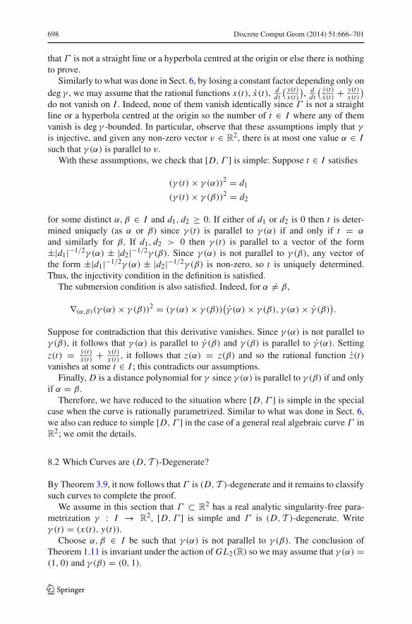
698 Discrete Comput Geom (2014) 51:666–701
that Γ is not a straight line or a hyperbola centred at the origin or else there is nothingto prove.
Similarly to what was done in Sect. 6, by losing a constant factor depending only ondeg γ , we may assume that the rational functions x(t), x(t), d
dt
( y(t)x(t)
), d
dt
( y(t)x(t) + y(t)
x(t)
)
do not vanish on I . Indeed, none of them vanish identically since Γ is not a straightline or a hyperbola centred at the origin so the number of t ∈ I where any of themvanish is deg γ -bounded. In particular, observe that these assumptions imply that γis injective, and given any non-zero vector v ∈ R
2, there is at most one value α ∈ Isuch that γ (α) is parallel to v.
With these assumptions, we check that [D, Γ ] is simple: Suppose t ∈ I satisfies
(γ (t)× γ (α))2 = d1
(γ (t)× γ (β))2 = d2
for some distinct α, β ∈ I and d1, d2 ≥ 0. If either of d1 or d2 is 0 then t is deter-mined uniquely (as α or β) since γ (t) is parallel to γ (α) if and only if t = α
and similarly for β. If d1, d2 > 0 then γ (t) is parallel to a vector of the form±|d1|−1/2γ (α) ± |d2|−1/2γ (β). Since γ (α) is not parallel to γ (β), any vector ofthe form ±|d1|−1/2γ (α) ± |d2|−1/2γ (β) is non-zero, so t is uniquely determined.Thus, the injectivity condition in the definition is satisfied.
The submersion condition is also satisfied. Indeed, for α �= β,
∇(α,β)(γ (α)× γ (β))2 = (γ (α)× γ (β))(γ (α)× γ (β), γ (α)× γ (β)
).
Suppose for contradiction that this derivative vanishes. Since γ (α) is not parallel toγ (β), it follows that γ (α) is parallel to γ (β) and γ (β) is parallel to γ (α). Settingz(t) = y(t)
x(t) + y(t)x(t) , it follows that z(α) = z(β) and so the rational function z(t)
vanishes at some t ∈ I ; this contradicts our assumptions.Finally, D is a distance polynomial for γ since γ (α) is parallel to γ (β) if and only
if α = β.Therefore, we have reduced to the situation where [D, Γ ] is simple in the special
case when the curve is rationally parametrized. Similar to what was done in Sect. 6,we also can reduce to simple [D, Γ ] in the case of a general real algebraic curve Γ inR
2; we omit the details.
8.2 Which Curves are (D, T )-Degenerate?
By Theorem 3.9, it now follows that Γ is (D, T )-degenerate and it remains to classifysuch curves to complete the proof.
We assume in this section that Γ ⊂ R2 has a real analytic singularity-free para-
metrization γ : I → R2, [D, Γ ] is simple and Γ is (D, T )-degenerate. Write
γ (t) = (x(t), y(t)).Choose α, β ∈ I be such that γ (α) is not parallel to γ (β). The conclusion of
Theorem 1.11 is invariant under the action of GL2(R) so we may assume that γ (α) =(1, 0) and γ (β) = (0, 1).
123
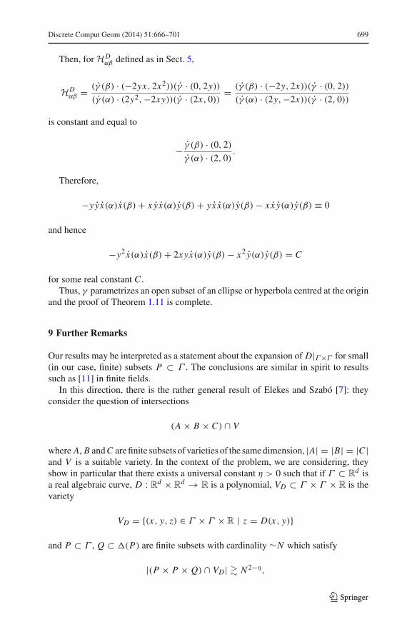
Discrete Comput Geom (2014) 51:666–701 699
Then, for HDαβ defined as in Sect. 5,
HDαβ = (γ (β) · (−2yx, 2x2))(γ · (0, 2y))
(γ (α) · (2y2,−2xy))(γ · (2x, 0))= (γ (β) · (−2y, 2x))(γ · (0, 2))
(γ (α) · (2y,−2x))(γ · (2, 0))
is constant and equal to
− γ (β) · (0, 2)
γ (α) · (2, 0).
Therefore,
−y yx(α)x(β)+ x yx(α)y(β)+ yx x(α)y(β)− x x y(α)y(β) ≡ 0
and hence
−y2 x(α)x(β)+ 2xyx(α)y(β)− x2 y(α)y(β) = C
for some real constant C .Thus, γ parametrizes an open subset of an ellipse or hyperbola centred at the origin
and the proof of Theorem 1.11 is complete.
9 Further Remarks
Our results may be interpreted as a statement about the expansion of D|Γ×Γ for small(in our case, finite) subsets P ⊂ Γ . The conclusions are similar in spirit to resultssuch as [11] in finite fields.
In this direction, there is the rather general result of Elekes and Szabó [7]: theyconsider the question of intersections
(A × B × C) ∩ V
where A, B and C are finite subsets of varieties of the same dimension, |A| = |B| = |C |and V is a suitable variety. In the context of the problem, we are considering, theyshow in particular that there exists a universal constant η > 0 such that if Γ ⊂ R
d isa real algebraic curve, D : R
d × Rd → R is a polynomial, VD ⊂ Γ × Γ × R is the
variety
VD = {(x, y, z) ∈ Γ × Γ × R | z = D(x, y)}
and P ⊂ Γ , Q ⊂ �(P) are finite subsets with cardinality ∼N which satisfy
|(P × P × Q) ∩ VD| � N 2−η,
123
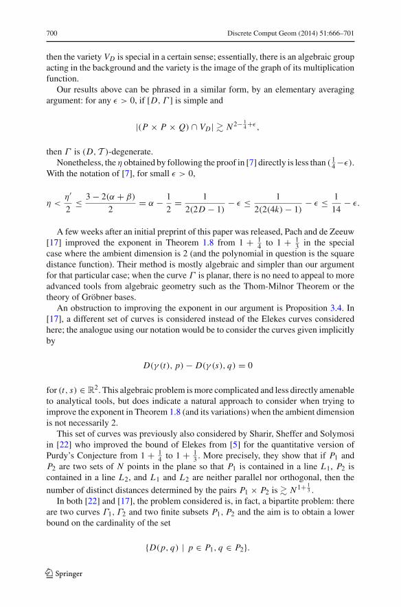
700 Discrete Comput Geom (2014) 51:666–701
then the variety VD is special in a certain sense; essentially, there is an algebraic groupacting in the background and the variety is the image of the graph of its multiplicationfunction.
Our results above can be phrased in a similar form, by an elementary averagingargument: for any ε > 0, if [D, Γ ] is simple and
|(P × P × Q) ∩ VD| � N 2− 14 +ε,
then Γ is (D, T )-degenerate.Nonetheless, the η obtained by following the proof in [7] directly is less than ( 1
4 −ε).With the notation of [7], for small ε > 0,
η <η′
2≤ 3 − 2(α + β)
2= α − 1
2= 1
2(2D − 1)− ε ≤ 1
2(2(4k)− 1)− ε ≤ 1
14− ε.
A few weeks after an initial preprint of this paper was released, Pach and de Zeeuw[17] improved the exponent in Theorem 1.8 from 1 + 1
4 to 1 + 13 in the special
case where the ambient dimension is 2 (and the polynomial in question is the squaredistance function). Their method is mostly algebraic and simpler than our argumentfor that particular case; when the curve Γ is planar, there is no need to appeal to moreadvanced tools from algebraic geometry such as the Thom-Milnor Theorem or thetheory of Gröbner bases.
An obstruction to improving the exponent in our argument is Proposition 3.4. In[17], a different set of curves is considered instead of the Elekes curves consideredhere; the analogue using our notation would be to consider the curves given implicitlyby
D(γ (t), p)− D(γ (s), q) = 0
for (t, s) ∈ R2. This algebraic problem is more complicated and less directly amenable
to analytical tools, but does indicate a natural approach to consider when trying toimprove the exponent in Theorem 1.8 (and its variations) when the ambient dimensionis not necessarily 2.
This set of curves was previously also considered by Sharir, Sheffer and Solymosiin [22] who improved the bound of Elekes from [5] for the quantitative version ofPurdy’s Conjecture from 1 + 1
4 to 1 + 13 . More precisely, they show that if P1 and
P2 are two sets of N points in the plane so that P1 is contained in a line L1, P2 iscontained in a line L2, and L1 and L2 are neither parallel nor orthogonal, then the
number of distinct distances determined by the pairs P1 × P2 is � N 1+ 13 .
In both [22] and [17], the problem considered is, in fact, a bipartite problem: thereare two curves Γ1, Γ2 and two finite subsets P1, P2 and the aim is to obtain a lowerbound on the cardinality of the set
{D(p, q) | p ∈ P1, q ∈ P2}.
123
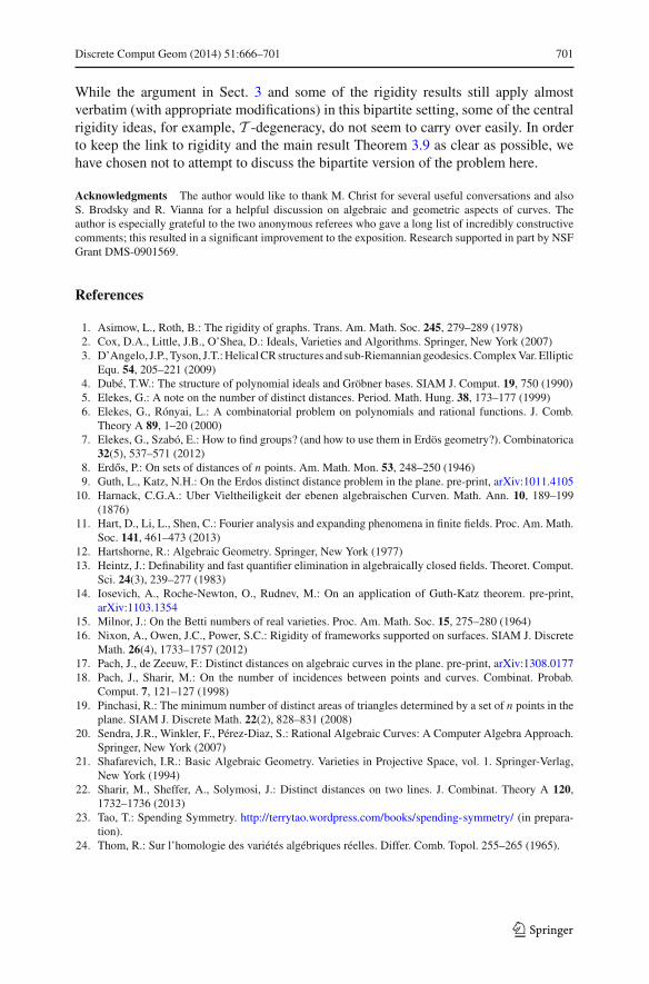
Discrete Comput Geom (2014) 51:666–701 701
While the argument in Sect. 3 and some of the rigidity results still apply almostverbatim (with appropriate modifications) in this bipartite setting, some of the centralrigidity ideas, for example, T -degeneracy, do not seem to carry over easily. In orderto keep the link to rigidity and the main result Theorem 3.9 as clear as possible, wehave chosen not to attempt to discuss the bipartite version of the problem here.
Acknowledgments The author would like to thank M. Christ for several useful conversations and alsoS. Brodsky and R. Vianna for a helpful discussion on algebraic and geometric aspects of curves. Theauthor is especially grateful to the two anonymous referees who gave a long list of incredibly constructivecomments; this resulted in a significant improvement to the exposition. Research supported in part by NSFGrant DMS-0901569.
References
1. Asimow, L., Roth, B.: The rigidity of graphs. Trans. Am. Math. Soc. 245, 279–289 (1978)2. Cox, D.A., Little, J.B., O’Shea, D.: Ideals, Varieties and Algorithms. Springer, New York (2007)3. D’Angelo, J.P., Tyson, J.T.: Helical CR structures and sub-Riemannian geodesics. Complex Var. Elliptic
Equ. 54, 205–221 (2009)4. Dubé, T.W.: The structure of polynomial ideals and Gröbner bases. SIAM J. Comput. 19, 750 (1990)5. Elekes, G.: A note on the number of distinct distances. Period. Math. Hung. 38, 173–177 (1999)6. Elekes, G., Rónyai, L.: A combinatorial problem on polynomials and rational functions. J. Comb.
Theory A 89, 1–20 (2000)7. Elekes, G., Szabó, E.: How to find groups? (and how to use them in Erdös geometry?). Combinatorica
32(5), 537–571 (2012)8. Erdos, P.: On sets of distances of n points. Am. Math. Mon. 53, 248–250 (1946)9. Guth, L., Katz, N.H.: On the Erdos distinct distance problem in the plane. pre-print, arXiv:1011.4105
10. Harnack, C.G.A.: Uber Vieltheiligkeit der ebenen algebraischen Curven. Math. Ann. 10, 189–199(1876)
11. Hart, D., Li, L., Shen, C.: Fourier analysis and expanding phenomena in finite fields. Proc. Am. Math.Soc. 141, 461–473 (2013)
12. Hartshorne, R.: Algebraic Geometry. Springer, New York (1977)13. Heintz, J.: Definability and fast quantifier elimination in algebraically closed fields. Theoret. Comput.
Sci. 24(3), 239–277 (1983)14. Iosevich, A., Roche-Newton, O., Rudnev, M.: On an application of Guth-Katz theorem. pre-print,
arXiv:1103.135415. Milnor, J.: On the Betti numbers of real varieties. Proc. Am. Math. Soc. 15, 275–280 (1964)16. Nixon, A., Owen, J.C., Power, S.C.: Rigidity of frameworks supported on surfaces. SIAM J. Discrete
Math. 26(4), 1733–1757 (2012)17. Pach, J., de Zeeuw, F.: Distinct distances on algebraic curves in the plane. pre-print, arXiv:1308.017718. Pach, J., Sharir, M.: On the number of incidences between points and curves. Combinat. Probab.
Comput. 7, 121–127 (1998)19. Pinchasi, R.: The minimum number of distinct areas of triangles determined by a set of n points in the
plane. SIAM J. Discrete Math. 22(2), 828–831 (2008)20. Sendra, J.R., Winkler, F., Pérez-Diaz, S.: Rational Algebraic Curves: A Computer Algebra Approach.
Springer, New York (2007)21. Shafarevich, I.R.: Basic Algebraic Geometry. Varieties in Projective Space, vol. 1. Springer-Verlag,
New York (1994)22. Sharir, M., Sheffer, A., Solymosi, J.: Distinct distances on two lines. J. Combinat. Theory A 120,
1732–1736 (2013)23. Tao, T.: Spending Symmetry. http://terrytao.wordpress.com/books/spending-symmetry/ (in prepara-
tion).24. Thom, R.: Sur l’homologie des variétés algébriques réelles. Differ. Comb. Topol. 255–265 (1965).
123