distortionary fiscal policy and monetary policy goals€¦ · distortionary fiscal policy and...
TRANSCRIPT

Distortionary Fiscal Policy and Monetary Policy Goals Klaus Adam and Roberto M. Billi
March 2010; Revised January 2011
RWP 10-10

Distortionary Fiscal Policy and Monetary Policy Goals1
Klaus Adam2 and Roberto M. Billi3
First version: March 2010 This version: January 2011
RWP 10-10
Abstract: We study interactions between monetary policy, which sets nominal interest rates, and fiscal policy, which levies distortionary income taxes to finance public goods, in a standard, sticky-price economy with monopolistic competition. Policymakers' inability to commit in advance to future policies gives rise to excessive inflation and excessive public spending, resulting in welfare losses equivalent to several percent of consumption each period. We show how appointing a conservative monetary authority, which dislikes inflation more than society does, can considerably reduce these welfare losses and that under optimal policy the monetary authority is mainly concerned about inflation. Full conservatism, i.e., exclusive concern about inflation, entirely eliminates the welfare losses from discretionary monetary and fiscal policymaking, provided monetary policy is determined after fiscal policy each period. Full conservatism, however, is severely suboptimal when monetary policy is determined simultaneously with fiscal policy or before fiscal policy each period. Keywords: discretion, Nash and Stackelberg equilibria, policy biases, sequential non-cooperative policy games
JEL classification: E52, E62, E63
1 We thank seminar participants at the Federal Reserve Bank of Kansas City, the Midwest Macroeconomics Meeting 2010 and the Society for Economic Dynamics Annual Meeting 2010. The views expressed herein are solely those of the authors and do not necessarily reflect the views of the Federal Reserve Bank of Kansas City or the Federal Reserve System. 2 Mannheim University, Department of Economics, L7, 3-5, 68131 Mannheim, Germany (and CEPR, London), email: [email protected] 3 Federal Reserve Bank of Kansas City, 1 Memorial Drive, Kansas City, MO 64198, United States, email: [email protected]

1 Introduction
The problem of designing institutional frameworks that cope best with discretionary behavior
of policymakers has received much attention following the seminal work of Kydland and
Prescott (1977) and Barro and Gordon (1983). In particular, to overcome the inflationary
bias caused by discretionary conduct of monetary policy, Rogoff (1985) proposed appointing
a “conservative”central banker, who dislikes inflation more than society does.
More recently, Adam and Billi (2008) have shown inflation conservatism à la Rogoff also
to be desirable in a setting with discretionary fiscal policy: besides overcoming the inflation-
ary bias, monetary conservatism can also eliminate the public-spending bias stemming from
discretionary public spending. But an unsatisfactory aspect of the analysis is the assumed
availability of lump-sum taxes, which contrasts with the observation that governments must
typically rely on distortionary tax instruments to raise revenue. Previous research, therefore,
ignored a key source of economic distortions associated with discretionary fiscal policy.
To address this shortcoming, this paper studies the interactions between discretionary
monetary and fiscal policy in a setting with distortionary taxes. Monetary policy sets nominal
interest rates and fiscal policy provides public goods, which are financed with a labor-income
tax that distorts labor-supply decisions. We conduct the analysis in a dynamic, general-
equilibrium model, with monopolistic competition and nominal rigidities. The presence of
monopoly power and distortionary income taxes causes output to fall below its first-best level
and provides discretionary policymakers an incentive to stimulate output.
We show analytically that discretionary fiscal policy gives rise to a public-spending bias
when prices are stable, while discretionary monetary policy gives rise to an inflationary bias.
In our numerical analysis we find these policy biases to be quantitatively important and also
an order of magnitude larger than in a setting with lump-sum taxes. This is so because
distortionary labor-income taxes amplify the effects of discretionary fiscal policy in a vicious
1

circle. A higher level of public spending requires higher taxes, which depress labor supply and
output. This in turn increases further the incentives for discretionary public spending. As a
consequence, also the welfare loss is found to be much larger than with lump-sum taxes and
is equivalent to a loss of several percent of consumption each period. This finding holds true
even when abstracting from the welfare costs of inflation.
In our general-equilibrium model of the economy, we then study the equilibrium outcomes
of a non-cooperative game between a discretionary fiscal authority, which maximizes social
welfare, and a discretionary monetary authority, which dislikes inflation more than society
does. We show that appointing such an inflation-conservative monetary authority can greatly
reduce the welfare loss due to discretionary policymaking and that a high degree of monetary
conservatism is optimal across a very wide range of model parameterizations. Monetary
conservatism can even entirely eliminate the steady-state distortions due to discretionary
monetary and fiscal policy when monetary policy can impose discipline on public spending
by moving after fiscal policy each period.
Although a high degree of monetary conservatism is found to be optimal for any timing
assumption on the sequence of moves between monetary an fiscal policy, exclusive focus on
inflation on the side of the monetary authority is optimal only when monetary policy moves
after fiscal policy each period. Otherwise, moving from the optimal (and high) degree of
conservatism to full conservatism gives rise to large welfare losses. As we show, after some
point the welfare gains from further inflation reductions are outweighed by the increasing
distortions in fiscal policy decisions that result from reduced inflation.
As a result, the addition of distortionary taxes is a crucial contribution since it overturns
the conclusions in Adam and Billi (2008). While full monetary conservatism is always a
good policy in a setting with lump-sum taxes, it can be a very bad policy in a setting with
distortionary taxes. A setting with lump-sum taxes leads to considerably understate the
costs of discretionary fiscal policy and to considerably overstate the benefits of full monetary
2
conservatism. Therefore, our setting with distortionary taxes reveals that it can be severely
suboptimal for the monetary authority to focus exclusively on inflation stabilization when
monetary policy is determined simultaneously with fiscal policy or before fiscal policy each
period.
The second section describes the model. The third section explains the policy biases.
The fourth section quantifies them. And the fifth section quantifies the effects of inflation
conservatism. Technical details are in the appendix.
2 The model
This section describes a sticky-price economy with monopolistic competition and separate
monetary and fiscal policy authorities. The setting is based on the model used in Adam
and Billi (2008), but relaxes the strong assumption of lump-sum taxes by considering instead
distortionary labor-income taxes. We first describe the private sector and the government and
thereafter define a private-sector equilibrium.
2.1 Private sector
There is a continuum of identical households with preferences given by
∞∑t=0
βtu(ct, ht, gt), (1)
where ct is consumption of an aggregate consumption good, ht ∈ (0, 1) is labor effort, gt is
public-goods provision by the government in the form of aggregate consumption goods, and
β ∈ (0, 1) is the discount factor. Utility is separable in c, h, and g. In addition, uc > 0, ucc < 0,
uh < 0, uhh ≤ 0, ug > 0, and ugg < 0. Furthermore,∣∣∣ cuccuc
∣∣∣ and ∣∣∣huhhuh
∣∣∣ are bounded.Each household produces a differentiated intermediate good. Demand for this good is
ytd(P̃t/Pt), where yt is (private and public) demand for the aggregate good, and P̃t/Pt is
the relative price of the intermediate good compared with the aggregate good. The demand
3
function d(·) satisfies d(1) = 1 and d′(1) = η, where η < −1 is the price elasticity of demand
for the different goods. The demand function is consistent with optimizing behavior when
private and public consumption goods are a Dixit-Stiglitz aggregate of the goods produced
by different households. Each household chooses P̃t, and hires labor effort h̃t to satisfy the
resulting product demand, i.e.,
h̃t = ytd
(P̃tPt
). (2)
As in Rotemberg (1982), sluggish nominal-price adjustment is described by quadratic-
resource costs of adjusting prices according to
θ
2
(P̃t
P̃t−1
− 1
)2
,
where θ > 0 indexes the degree of price stickiness.1
Households’budget constraint is
Ptct +Bt = Rt−1Bt−1 + Pt
P̃tPtytd
(P̃tPt
)− wth̃t −
θ
2
(P̃t
P̃t−1
− 1
)2+ Ptwtht(1− τt), (3)
where Rt ≥ 1 is the gross nominal interest rate.2 Bt are private-issued nominal bonds paying
RtBt in period t + 1, wt is the real wage paid in a competitive labor market, and τt is a
(distortionary) labor-income tax rate. Instead of labor-income taxes, we could have considered
taxes on total income (profits and labor income) or consumption taxes. As is well known,
consumption taxes are equivalent to having a labor-income tax together with a lump-sum
tax on profits. We decided to analyze the most distortionary tax system, so we consider
labor-income taxes.
Finally, the no-Ponzi-scheme constraint is
limj→∞
t+j−1∏i=0
1
Ri
Bt+j ≥ 0. (4)
1Using the Calvo approach to describe nominal rigidities would complicate considerably the analysis, be-
cause then price dispersion becomes an endogenous state variable.2We abstract from money holdings and seigniorage by considering a “cashless-limit”economy à la Woodford
(1998). Hence, money only imposes a zero lower bound on nominal interest rates, i.e., Rt − 1 ≥ 0 for all t.
4

Based on these assumptions, households’problem consists of choosing {ct, ht, h̃t, P̃t, Bt}∞t=0,
so to maximize (1), subject to (2)-(4), and taking {yt, Pt, wt, Rt, gt, τt}∞t=0 as given. The first-
order conditions of this problem are (2)-(4) holding with equality, and
−uhtuct
=wt(1− τt) (5)
uctRt
=βuct+1
Πt+1
0 =uct
[ytd(rt) + rtytd
′(rt)−wtztytd′(rt)− θ
(Πt
rtrt−1
− 1
)Πt
rt−1
]+ βθuct+1
(rt+1
rtΠt+1 − 1
)rt+1
r2t
Πt+1,
where rt ≡ P̃tPtdenotes the relative price and Πt ≡ Pt
Pt−1the gross inflation rate. Equation (5)
shows that labor-income taxes distort the marginal rate of substitution between leisure and
consumption.
In addition to the equations above, a transversality condition, limj→∞ (βt+juct+jBt+j/Pt+j) =
0, has to hold at all contingencies. We assume private-issued bonds are in zero aggregate net
supply, so the transversality condition is always satisfied. The same applies to the no-Ponzi-
scheme constraint (4).
2.2 Government
The government consists of two authorities, namely a monetary authority controlling short-
term nominal interest rates Rt and a fiscal authority determining public-goods provision gt
and income-tax rates τt in each period t.3
The government cannot credibly commit in advance to future policies or to repay debt in
the future, i.e., it operates under full discretion. As a consequence, public-goods provision
3Of course, monetary policy controls the nominal interest rate by adjusting the money supply. This requires
that it owns a stock of private bonds to perform the necessary open market operations. Since we consider a
cashless-limit economy, as in Woodford (1998), the required stock of bonds is infinitesimally small, allowing
us to assume that monetary policy controls directly nominal interest rates.
5
must be financed with current taxes only and the government’s balanced-budget constraint is
τtwtht = gt. (6)
As a benchmark, we will also consider a Ramsey equilibrium in which the government
commits in advance to future policies and thereby could credibly promise to repay debt. Yet
to facilitate comparison, we will still impose the balanced-budget constraint (6) and set the
initial level of government-issued debt equal to zero.4
2.3 Private-sector equilibrium
We consider a symmetric price-setting equilibrium in which the relative price rt is equal to
1 for all t. It follows that, the first-order conditions describing households’behavior can be
condensed into a price-setting equation, i.e., a Phillips curve
uct(Πt − 1)Πt =ucthtθ
(1 + η + η
(uhtuct− gtht
))+ βuct+1(Πt+1 − 1)Πt+1, (7)
and a consumption-Euler equation
uctRt
= βuct+1
Πt+1
. (8)
Conveniently, the last two equations do not make reference to taxes and real wages. Rather
these are determined by (5) and (6) which give
τt =gt
gt − ht uhtuct
(9)
wt =gtht− uhtuct
. (10)
A private-sector equilibrium, therefore, consists of a plan {ct, ht,Πt} satisfying (7), (8),
and a market-clearing condition (resource constraint)
ht = ct +θ
2(Πt − 1)2 + gt, (11)
4The absence of government-issued debt implies we abstract from monetary and fiscal interactions operating
directly through the government’s budget constraint, see Díaz-Giménez et al. (2008).
6

taking policies {gt, Rt ≥ 1} as given.5
3 Policy regimes and biases
In this section, we study policy regimes with and without commitment to future policies and
the associated equilibrium allocations. We start by studying the first-best allocation, which
assumes policy commitment and abstracts from monopoly and tax distortions and nominal
rigidities. We then study a Ramsey allocation, which accounts for monopoly distortions,
nominal rigidities, and distortionary labor-income taxes. Finally, we relax the assumption of
policy commitment and study allocations under sequential policymaking, taking into account
all aforementioned distortions. We show that sequential-fiscal policy causes too much public
spending, while sequential-monetary policy causes too much inflation.
3.1 First-best and Ramsey allocation
The first-best allocation, which abstracts from all distortions and commitment problems,
satisfies in steady state the following condition:6
uc = ug = −uh.
It is thus optimal to equate the marginal utility of private and public consumption to the
marginal disutility of labor effort. This condition follows directly from the linearity of the
production function and the preference structure. As we show next, the condition is no longer
optimal when the distortions in the economy are taken into account even if policymakers can
credibly commit.
5The initial price level P−1 can be ignored, because it only normalizes the price-level path.6The condition follows from solving max{ct,ht,gt}∞t=0
∑∞t=0 β
tu(ct, ht, gt), subject to (11) with θ = 0 and
from imposing on the resulting first-order conditions a steady-state restriction.
7

The Ramsey allocation, which accounts for tax and monopoly distortions and nominal
rigidities, must satisfy the implementability constraints (7) and (8) and the resource constraint
(11). It solves the following problem:
max{ct,ht,Πt,Rt≥1,gt}∞t=0
∞∑t=0
βtu(ct, ht, gt) (12)
subject to (7), (8), and (11) for all t.
Note, the Ramsey allocation still allows for advance-policy commitment. The first-order
conditions of this problem show that the Ramsey steady state satisfies
Π = 1 and R =1
β, (13)
as well as marginal conditions
−uh < ug (14)
−uh =
(1 + η
η− g
h
)uc. (15)
See appendix A.1 for derivations. Equation (13) shows that it is optimal to achieve price
stability. In addition, (14) shows that public spending in the Ramsey allocation falls short
of its first-best level. This is optimal because public spending increases taxes and thereby
the wedge between the marginal utility of private consumption and the marginal disutility of
labor effort, see equation (15). This wedge has two components. The first component is due to
the monopoly power of firms, which causes real wages to fall short of their marginal product.7
The second component– which is missing in the setting of Adam and Billi (2008)– stems from
distortionary labor-income taxes levied to finance public spending. Reducing public spending
below the first-best level lowers taxes and reduces this wedge.
7Equations (10) and (15) imply w = (1 + η) /η < 1.
8

3.2 Sequential-policy regimes
We now study separate monetary and fiscal authorities that cannot commit in advance to
future policies and, instead, decide policies sequentially at the time of implementation. We
derive a policy-reaction function for each authority. To facilitate the exposition, we assume
each authority takes the current policy of the other authority and all future private-sector
and policy decisions as given. We then verify the rationality of this assumption and define a
sequential-policy equilibrium.
3.2.1 Sequential-fiscal policy: spending bias
Based on the assumptions made, the fiscal authority’s problem in period t is
max(ct,ht,Πt,gt)
∞∑j=0
βju(ct+j, ht+j, gt+j) (16)
subject to (7), (8), and (11) for all t
and {ct+j, ht+j,Πt+j, Rt+j−1 ≥ 1, gt+j} given for j ≥ 1.
In this problem the fiscal authority takes current monetary policy Rt and future decisions
as given. Eliminating Lagrange multipliers from the first-order conditions of the problem
delivers a fiscal-reaction function
ugt = −uht2Πt − 1− η(Πt − 1)
2Πt − 1− (Πt − 1)(
1 + η + η uhtuct
+ ηhtuhhtuct
) . (FRF)
See appendix A.2 for the derivation. This FRF determines (implicitly) the optimal level
of public-goods provision gt in each period t under sequential-fiscal policy.
To study the implications of sequential-fiscal policy, consider a steady state in which policy
achieves price stability (Π = 1) as in the Ramsey allocation. The FRF then simplifies to
ug = −uh. (17)
9

Under price stability, fiscal policy thus equates the marginal utility of public consumption to
the marginal disutility of labor effort. Such behavior is consistent with the first-best allocation,
but suboptimal in the presence of tax and monopoly distortions that require reducing public
spending below its first-best level, see the Ramsey optimality condition (14). Sequential-fiscal
policy, therefore, causes a “spending bias”as summarized in the following proposition:
Proposition 1 Sequential-fiscal policy under price stability causes a spending bias.
The intuition for this finding is as follows. Since fiscal policy takes future allocations
and the monetary policy decision Rt as given, the Euler equation (8) implies that private
consumption is equally perceived as given. A discretionary fiscal policymaker thus perceives
to affect labor supply one-for-one with public spending and to have no distortionary effects on
private consumption, which implies rule (17) is optimal. But in equilibrium future spending
and tax decisions do affect future labor supply and future private consumption. Low future
consumption then adversely affects current consumption via the anticipation effects implicit
in the Euler equation. But a discretionary policymaker does not perceive the effects that
current policy have on past decisions of forward-looking households.
In general when price stability is not achieved, the fiscal policymaker also takes into account
that any additional public spending increases inflation and that this involves non-zero marginal
resource costs.8 These marginal resource costs of inflation therefore lead to the more general
expression FRF.
8Recall that fiscal policy perceives output to move one-for-one with public spending, because it perceives
private consumption as given. Therefore public spending implies an increase in wages and, via the Phillips
curve (7), an increase in inflation.
10
3.2.2 Sequential-monetary policy: inflation bias
The monetary authority’s problem in period t is
max(ct,ht,Πt,Rt≥1)
∞∑j=0
βju(ct+j, ht+j, gt+j) (18)
subject to (7), (8), and (11) for all t
and {ct+j, ht+j,Πt+j, Rt+j ≥ 1, gt+j−1} given for j ≥ 1.
In this problem the monetary authority takes current fiscal policy gt and future decisions
as given. Eliminating Lagrange multipliers from the first-order conditions of the problem
delivers a monetary-reaction function
− uctuht
(η (Πt − 1)− Πt)− (Πt − 1) η
(1 + ht
uhhtuht
)+ 2Πt − 1− ucct
uct(Πt − 1)
(θ(Πt − 1)Πt − ht
(1 + η − η gt
ht
))= 0. (MRF)
Appendix A.3 shows the derivation. This MRF determines (implicitly) the optimal level
of nominal interest rates Rt in each period t under sequential-monetary policy.
Consider again a steady state in which policy achieves price stability (Π = 1) as in the
Ramsey allocation. MRF then simplifies to
uc = −uh.
Under price stability, monetary policy thus equates the marginal utility of private con-
sumption to the marginal disutility of labor effort. Again such behavior is consistent with
the first-best allocation and suboptimal in the presence of monopoly and tax distortions, see
the Ramsey optimality condition (15). Monetary policy thus seeks to increase output above
the Ramsey steady state and the MRF is actually inconsistent with price stability. Therefore
sequential-monetary policy causes an “inflation bias,”as in the standard case with exogenous
fiscal policy studied, for example, in Svensson (1997) and in Walsh (1995). This result is
captured in the following proposition, which is formally proven in appendix A.4:
11
Proposition 2 Sequential-monetary policy causes an inflationary bias: the steady-state gross
inflation rate Π is strictly bigger than 1, provided the discount factor β is suffi ciently close to
1.
3.2.3 Sequential-policy (SP) equilibrium
We now define a sequential-policy equilibrium. We start by verifying the rationality of the
assumption we made that each authority can take the current policy of the other authority
and all future decisions as given. When solving the fiscal authority’s problem (16) and the
monetary authority’s problem (18), we observe (7), (8), and (11) depend on current and future
decisions only.9 This observation suggests the existence of an equilibrium in which indeed
current policy is independent of past decisions and, in turn, future policy is independent of
current decisions. Also the resulting policy-reaction functions FRF and MRF then depend on
current decisions only.
Based on these considerations, we can formally define a Markov-perfect Nash equilibrium
under sequential monetary and fiscal policy.10 In such a Nash equilibrium, the monetary
and fiscal authorities decide their respective policies simultaneously in each period with each
authority deciding policy based on its own policy-reaction function:
Definition 3 (SP) A Markov-perfect Nash equilibrium under sequential monetary and fiscal
policy is a steady state {c, h,Π, R ≥ 1, g} satisfying (7), (8), (11), FRF, and MRF.
Importantly, the assumption of simultaneous-policy decisions does not matter for the equi-
librium outcome. This is because the monetary and fiscal authorities share the same objective
function.11 In section 5, where the two authorities pursue different objectives due to mone-
9There are no state variables in the model.10The concept of Markov-perfect equilibrium, as defined in Maskin and Tirole (2001), figures prominently
in applied game theory. See for example Klein, Krusell, and Ríos-Rull (2008).11Consider a Stackelberg game in which one authority decides before the other each period. Then, provided
both players share the same policy objective, the follower’s policy-reaction function does not need to be
12
tary conservatism, the (within-period) timing of policy decisions will start to matter for the
equilibrium outcome.
4 How much inflation is optimal?
We have shown sequential-fiscal policy spends too much on public goods, while sequential-
monetary policy gives rise to an inflation bias. In this section, we quantify these policy
biases. As a point of reference, we first describe an optimal-inflation regime in which the
monetary authority is capable of advance-policy commitment, but fiscal policy follows the
reaction function FRF. We then determine the equilibrium outcome without monetary and
fiscal policy commitment in a calibrated version of the model. Comparing the outcome in this
latter setting with that in the optimal-inflation regime, we argue that installing an inflation-
conservative central bank is desirable for society as it may result in large welfare gains.
4.1 Optimal-inflation (OI) regime
This section considers an intermediate policy problem in which the monetary authority can
commit in advance to future policies, while the fiscal authority determines its actions according
to the reaction function FRF. This policy problem is of interest because it allows to determine
the welfare-optimal inflation rate in the presence of discretionary fiscal policy. The policy
problem is
max{ct,ht,Πt,Rt≥1,gt}∞t=0
∞∑t=0
βtu(ct, ht, gt) (OI)
subject to (7), (8), (11), and FRF for all t.
And we refer to it as the optimal-inflation (OI) regime. In this regime, the monetary
authority sets an equilibrium inflation rate which accounts for the fiscal authority’s inability
imposed as a constraint in the leader’s problem. Rather, it can be derived directly from the leader’s first-order
conditions.
13

to commit in advance to future policies.12 It contrasts with the sequential-policy (SP) regime,
described in the previous section, which also accounts for the monetary authority’s inability to
commit. If inflation in the OI regime lies below that emerging in the SP regime, this suggests
inflation conservatism is desirable to the extent that it is effective in lowering the equilibrium
inflation rate in the economy.
4.2 Calibration
We now turn to numerical results. We calibrate the model as in Adam and Billi (2008), so to
make the results comparable. Accordingly, household preferences are specified as
u(ct, ht, gt) = log (ct)− ωhh1+ϕt
1 + ϕ+ ωg log (gt) , (19)
where ωh > 0, ωg ≥ 0, and ϕ ≥ 0.13
The baseline parameter values are shown in table 1. In the baseline, the discount factor
β is equal to 0.9913 quarterly, which implies a real interest rate of 3.5 percent annually. The
price elasticity of demand η is equal to −6, so the mark-up of prices over marginal costs is
20 percent.14 The degree of price stickiness θ is equal to 17.5, so the log-linearized version
of Phillips curve (7) is consistent with that in Schmitt-Grohé and Uribe (2004). And the
labor-supply elasticity ϕ−1 is equal to 1. In addition, we set the utility weights ωh and ωg
such that in the Ramsey allocation agents work 20 percent of their time (h equal to 0.2) and
spend 20 percent of output on public goods (g equal to 0.04).15 Thereby the labor-income tax
rate τ is 24 percent.
We tested the robustness of the numerical results across a wide range of parameter values,
and by using in the numerical procedure different starting values for the allocation. As we
12In steady state, equation (8) implies Π = βR. Thereby the monetary authority, by setting the gross
nominal interest rate R, determines the gross inflation rate Π.13This specification is consistent with balanced growth.14The mark-up µ is given by 1 + µ = η/ (1 + η).15We set the utility weights using (47) and (51) in appendix A.5.
14

will show below, the results are found to be robust.16
4.3 Quantifying policy biases
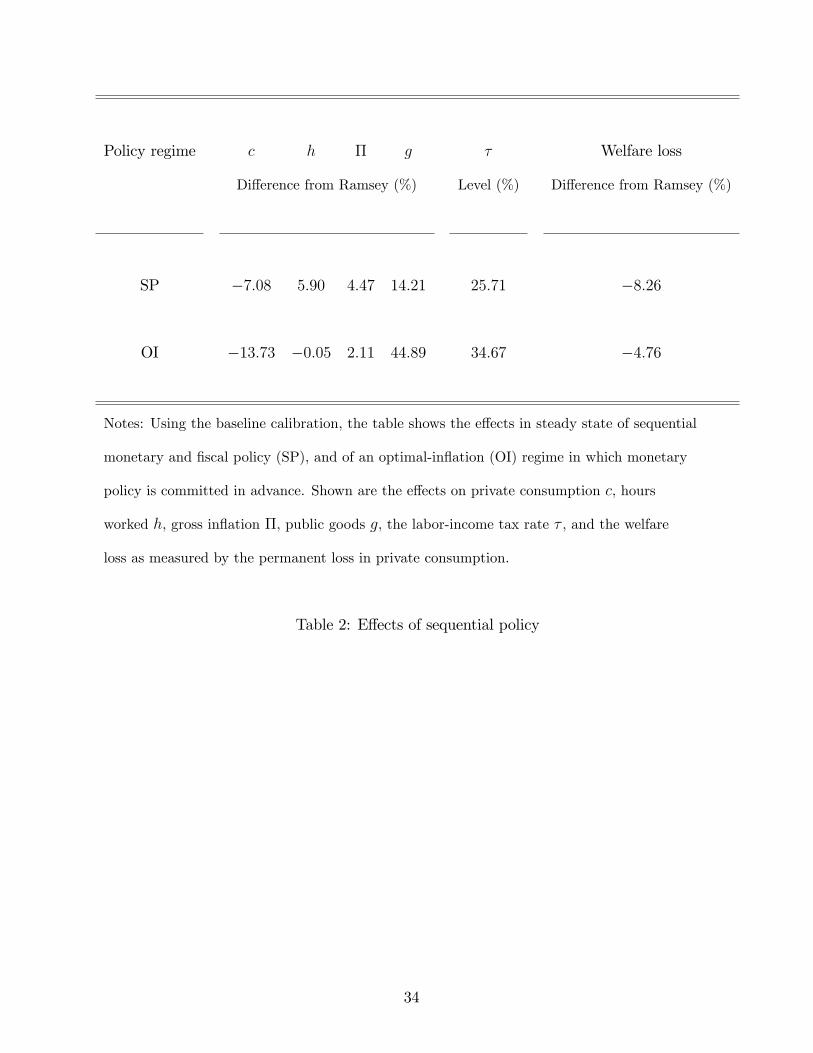
The effects of sequential policy under the baseline parameterization are shown in table 2. The
second column shows the effects on the equilibrium allocation, i.e., on private consumption
c, hours worked h, gross inflation Π, and public goods g. These effects are measured as the
difference from the Ramsey allocation.17 The third column shows the labor-income tax rate.
And the last column shows the welfare loss as measured by the permanent loss in private
consumption compared with the Ramsey allocation.18
The effects in the SP regime are shown in the first row of table 2. In such a regime, the
inflation bias is found to be sizable. In fact, inflation is roughly 4.5 percent higher than in
the Ramsey allocation. Also the spending bias is found to be sizable, with spending on public
goods roughly 14 percent higher than in the Ramsey allocation. Overall, therefore, the welfare
loss due to sequential policy is big, and equivalent to foregoing more than 8 percent of private
consumption each period compared with the Ramsey allocation. Although about 80 percent
of the welfare loss is due to the resource costs of inflation, the remaining 20 percent of the loss
is due to distorted allocations between hours worked, private consumption, and public goods.
The latter 20 percent of the loss is equivalent to foregoing 1.6 percent of consumption each
period. Therefore the welfare losses is large by conventional standards even when abstracting
from the resource costs of inflation.16To make the Ramsey allocation invariant to changes in parameter values, we adjust the utility weights ωh
and ωg. Using different starting values for the allocation, we did not encounter multiplicities in the equilibrium
allocation under any of the policy regimes.17In the Ramsey allocation c = 0.16, h = 0.2, Π = 1, g = 0.04, and τ = 0.24.18More specifically, the welfare loss is measured as the permanent reduction in private consumption that
would make welfare in the Ramsey allocation equivalent to welfare in the policy regime considered. See
appendix A.6.
15

The effects in the OI regime are shown in the second row of table 2. In this regime, the
inflation bias remains sizable, but is less than half of that in the SP regime. The fact that
the optimal inflation rate in the OI regime is below the inflation bias emerging in the SP
regime indicates that indeed inflation conservatism would be desirable for society. Moreover,
the welfare loss in the OI regime is about one half of that in the SP regime, which suggests
that inflation conservatism may result in large welfare gains. Interestingly, the fiscal spending
bias increases roughly by a factor of three compared to the SP regime. This is because lower
inflation reduces the fiscal authority’s perceived costs of public spending, as discussed before.19
Despite the high level of public spending, hours worked in the OI regime are roughly the same
as in the Ramsey allocation. Now only about 30 percent of the welfare loss is due to the
resource costs of inflation, while the remaining 70 percent of the loss is largely due to the
distortion in the allocation between private consumption and public goods. The latter 70
percent of the loss now amounts to foregoing 3.3 percent of consumption each period, which
indeed is large by conventional standards.
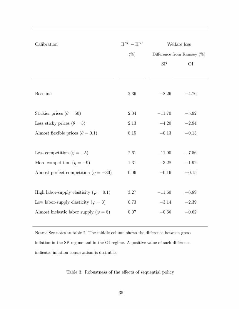
These findings are robust across a wide range of parameter values. The last two columns
of table 3 show that the potential welfare gains from inflation conservatism remain sizable
across a wide range of model parameterizations. They disappear, however, in the limiting
cases when prices become flexible (θ suffi ciently close to zero), when goods markets become
competitive (η suffi ciently low), and when labor supply becomes inelastic (ϕ suffi ciently high).
Still, the optimal inflation rate in the OI regime lies below that in the SP regime for all the
parameterizations, see the second column of table 3. This suggests that inflation conservatism
remains desirable across a wide range of model parameterizations.
19This effect can be shown analytically in a setting in which taxes are lump sum, see Adam and Billi (2008).
16

5 Conservative monetary authority
The previous section has shown that lowering inflation below the outcome emerging with
sequential monetary and fiscal policy is highly desirable in welfare terms. In this section,
we introduce an inflation-conservative monetary authority and asses to what extent inflation
conservatism can deliver these welfare gains when both policymakers continue to determine
policy sequentially. We consider three policy regimes, namely regimes in which monetary
policy is decided before, simultaneously, or after fiscal policy within each period. We show that
inflation conservatism is particularly desirable when fiscal policy is decided before monetary
policy as it is then possible to recover the Ramsey steady state, despite both policymakers
acting sequentially.
5.1 Inflation conservatism
As in Rogoff(1985) and in Adam and Billi (2008), we consider a sequential-monetary authority
that not only cares about society’s welfare, but also dislikes inflation directly. We model this
by replacing the monetary authority’s objective in each period t with a more general, inflation-
conservative objective
(1− α)u(ct, ht, gt)− α(Πt − 1)2
2, (20)
where α ∈ [0, 1]measures the degree of the monetary authority’s inflation conservatism. When
α is equal to zero the monetary authority cares about society’s welfare only, as assumed in the
analysis so far. When α is strictly bigger than zero the monetary authority dislikes inflation
more than suggested by social preferences, and as α approaches 1 the monetary authority
starts to become exclusively concerned about inflation.
The fiscal authority continues to be concerned about social welfare only, i.e., the objective
of the fiscal authority remains unchanged. With monetary and fiscal authorities no longer
17
pursuing the same policy objective, the (within-period) timing of policy decisions now matters
for the equilibrium outcome. Therefore we consider a Nash equilibrium and also Stackelberg
equilibria with monetary and fiscal leadership.
5.2 Nash equilibrium
We start by considering the policy regime in which the monetary and fiscal authorities decide
policies simultaneously each period. In such a Nash regime, the fiscal authority’s problem
remains unchanged and continues to take the monetary policy decision as given. Fiscal be-
havior thus continues to be described by the reaction function FRF. However, the monetary
authority’s problem in period t is now given by
max(ct,ht,Πt,Rt≥1)
∞∑j=0
βj[(1− α)u(ct+j, ht+j, gt+j)− α
(Πt+j − 1)2
2
](21)
subject to (7), (8), and (11) for all t
and {ct+j, ht+j,Πt+j, Rt+j ≥ 1, gt+j−1} given for j ≥ 1.
In this problem the monetary authority still takes current fiscal policy gt and future deci-
sions as given. Eliminating Lagrange multipliers from the first-order conditions of the problem
delivers a conservative monetary-reaction function
− uctuht
(η (Πt − 1)− Πt)− (Πt − 1) η
(1 + ht
uhhtuht
)+
[2Πt − 1− ucct
uct(Πt − 1)
(θ(Πt − 1)Πt − ht
(1 + η − η gt
ht
))](1− α) θ − α 1
uht
(1− α) θ + α 1uct
= 0.
(CMRF)
See appendix A.7 for the derivation. When α is equal to zero CMRF simplifies to MRF,
which is the monetary-reaction function without inflation conservatism. As before, CMRF
18

still depends on current decisions only. Therefore it continues to be rational to take the
current policy of the other authority and all future decisions as given. We can then define a
Markov-perfect Nash equilibrium with conservative monetary policy as follows:
Definition 4 (CSP-Nash) A Markov-perfect Nash equilibrium with conservative and se-
quential monetary policy, sequential-fiscal policy, and simultaneous-policy decisions is a steady
state {c, h,Π, R ≥ 1, g} satisfying (7), (8), (11), FRF, and CMRF.
5.3 Stackelberg equilibria
We now consider Stackelberg equilibria where one of the policymakers decides before the other
each period. We start by considering a setting with monetary leadership (ML). Again, since
the fiscal authority takes monetary decisions as given, its policy problem remains unchanged
and its optimal behavior is described by the reaction function FRF. The monetary authority,
however, takes into account FRF as an additional constraint, and its problem in period t
becomes
max(ct,ht,Πt,gt,Rt≥1)
∞∑j=0
βj[(1− α)u(ct+j, ht+j, gt+j)− α
(Πt+j − 1)2
2
](22)
subject to (7), (8), (11), and FRF for all t
and {ct+j, ht+j,Πt+j, Rt+j ≥ 1, gt+j} given for j ≥ 1.
In this problem the monetary authority still takes future decisions as given, but now
anticipates how its choices affect the current fiscal-policy decision. Eliminating Lagrange
multipliers from the first-order conditions of the problem delivers a conservative monetary-
reaction function under monetary leadership, which we denote as CMRF-ML. The resulting
equilibrium definition then is the following:
Definition 5 (CSP-ML) A Markov-perfect Stackelberg equilibrium with conservative and
sequential monetary policy, sequential-fiscal policy, and monetary policy decided before fiscal
19

policy is a steady state {c, h,Π, R ≥ 1, g} satisfying (7), (8), (11), FRF, and CMRF-ML.
Next, consider the opposite setting with fiscal leadership (FL). Since the monetary author-
ity decides second, it takes fiscal decisions as given. Therefore its reaction function continues
to be CMRF, which needs to be imposed as a constraint on the fiscal authority’s problem
max(ct,ht,Πt,gt,Rt≥1)
∞∑j=0
βju(ct+j, ht+j, gt+j) (23)
subject to (7), (8), (11), and CMRF for all t
and {ct+j, ht+j,Πt+j, Rt+j ≥ 1, gt+j} given for j ≥ 1.
In this problem the fiscal authority still takes future decisions as given, but anticipates
the within-period reaction of nominal interest rates Rt as implied by CMRF. Eliminating
Lagrange multipliers from the first-order conditions of the problem delivers a conservative
fiscal-reaction function under fiscal leadership, which we denote as CFRF-FL. The resulting
Markov-perfect Stackelberg equilibrium is defined as follows:
Definition 6 (CSP-FL) A Markov-perfect Stackelberg equilibrium with conservative and se-
quential monetary policy, sequential-fiscal policy, and fiscal policy decided before monetary
policy is a steady state {c, h,Π, R ≥ 1, g} satisfying (7), (8), (11), CFRF-FL, and CMRF.
5.4 Effects of inflation conservatism
We now discuss the different policy regimes and compare the effects of inflation conservatism.
In the Nash and ML regimes, the fiscal authority’s reaction function is given by FRF. As a
consequence, welfare in these regimes cannot exceed that of the OI regime. The situation
is different in the FL regime where the fiscal authority anticipates within each period the
monetary authority’s inflation conservatism. This regime allows monetary conservatism to
discipline the behavior of the fiscal authority, and thereby welfare may end up higher than in
the OI regime.
20

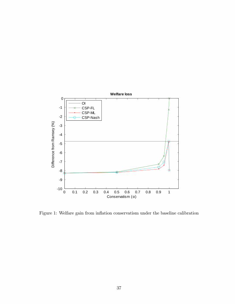
Using the baseline parameterization, figure 1 shows the welfare gain from inflation conser-
vatism. The figure shows the consumption-equivalent welfare losses (vertical axis) in deviation
from the Ramsey outcome as a function of the degree of inflation conservatism α (horizontal
axis). Besides showing the outcome under the three different timing protocols, the figure also
shows a solid-horizontal line that corresponds to the welfare loss in the OI regime.
In the Nash and ML regimes, welfare increases with the degree of inflation conservatism
and a value of α just slightly below 1 recovers the level of welfare in the OI regime. But
increasing α all the way to 1 causes a steep welfare loss relative to the OI regime, which
shows that full inflation conservatism (α = 1) is not optimal under these timing protocols.
An explanation for this non-monotone effect is provided below.
Regarding the FL regime, welfare again increases with α, but now monotonically, and
reaches the Ramsey-steady-state level as α is increased all the way to 1. With fiscal leadership,
therefore, full inflation conservatism eliminates the steady-state distortions associated with
lack of monetary and fiscal commitment.
Overall, figure 1 suggests that inflation conservatism is desirable, because then welfare
is always higher, for all timing protocols and for all values of α. With monetary leadership
and with simultaneous policy decisions, however, it is not optimal for monetary policy to be
exclusively concerned about inflation stabilization (α = 1). The reason for this finding can be
uncovered by considering the allocational effects of different degrees of inflation conservatism
under the different timing protocols.
Again using the baseline parameterization, figure 2 shows the effects of different degrees
of inflation conservatism (horizontal axis) on the equilibrium outcomes. As shown, inflation
conservatism unambiguously lowers the equilibrium inflation rate (lower-left panel) and hours
worked (top-right panel). The latter effect occurs partly because lower inflation gives rise to
lower resource costs.
The effects on the fiscal-spending bias (lower-right panel), however, depend crucially on
21
whether the fiscal authority internalizes the monetary authority’s direct reaction to inflation,
i.e., on whether fiscal policy moves before monetary policy. Inflation conservatism reduces the
fiscal-spending bias in the FL regime but increases it strongly in the Nash and ML regimes,
which results in large welfare losses as α approaches 1.
This divergence in outcomes can be rationalized as follows. As explained above, inflation
conservatism lowers the equilibrium inflation rate. As a result, it also lowers the marginal
resource costs of inflation, so the perceived costs of additional inflation caused by additional
public spending are equally lower. Therefore when fiscal policy takes monetary policy as given,
as in the Nash and ML regimes, lower inflation induces the fiscal authority to increase public
spending. But in the FL regime the fiscal authority anticipates that higher public spending
will come at the cost of higher nominal interest rates, because the monetary authority will
tighten monetary policy to partially offset a rise in inflation. The consumption Euler equation
(8) then implies that the fiscal authority perceives that public spending crowds out private
consumption in the current period. Indeed for α equal to 1 the fiscal authority anticipates that
higher public spending lowers private consumption one-for-one, as monetary policy does not
tolerate any inflation and any change in hours worked. Fiscal policy then correctly perceives
the one-for-one trade-off between private consumption and public spending as implied by the
production function. Therefore fiscal policy implements the Ramsey level of public spending
even though it lacks the ability to commit to future policies.
Table 4 displays the optimal degree of inflation conservatism (αopt) for the Nash and ML
regimes and a wide range of model parameterizations. It shows that, independently from
the precise parameter values, the central bank should predominantly be concerned about
inflation in these regimes. At the same time, however, increasing monetary conservatism to
the maximum degree (α = 1) is severely suboptimal. As the last two columns table 4 show,
such a move is typically associated with welfare losses that are equivalent to several percentage
points of consumption each period. The findings from the baseline calibration are thus robust
22
across many model parameterizations.
6 Conclusions
We study interactions between discretionary monetary and fiscal policymakers when monetary
policy sets nominal interest rates and fiscal policy provides public goods that are financed with
distortionary taxes. The welfare loss resulting from sequential policymaking is found to be
equivalent to foregoing several percent of private consumption each period. This welfare loss,
however, can be largely reduced and even eliminated by appointing a conservative monetary
authority, who dislikes inflation more than society does.
A high degree of inflation conservatism is found to be optimal for any timing assumption on
the sequence of moves in the non-cooperative game between monetary and fiscal policymak-
ers. But it is severely suboptimal for the monetary authority to focus exclusively on inflation
stabilization when the fiscal authority fails to anticipate that its policy decision affects the
monetary authority’s interest-rate decision. When such anticipation of policy interactions oc-
curs, the monetary authority should focus exclusively on inflation stabilization. Full inflation
conservatism then eliminates the steady-state distortions associated with lack of monetary
and fiscal commitment.
References
Adam, K., and R. Billi (2008): “Monetary Conservatism and Fiscal Policy,” Journal of
Monetary Economics, 55, 1376—1388.
Barro, R., and D. B. Gordon (1983): “A Positive Theory of Monetary Policy in a Natural
Rate Model,”Journal of Political Economy, 91, 589—610.
23

Díaz-Giménez, J., G. Giovannetti, R. Marimon, and P. Teles (2008): “Nominal Debt
as a Burden on Monetary Policy,”Review of Economic Dynamics, 11, 493—514.
Klein, P., P. Krusell, and J.-V. Ríos-Rull (2008): “Time Consistent Public Policy,”
Review of Economic Studies, 75, 789—808.
Kydland, F. E., and E. C. Prescott (1977): “Rules Rather Than Discretion: The
Inconsistency of Optimal Plans,”Journal of Political Economy, 85, 473—492.
Maskin, E., and J. Tirole (2001): “Markov Perfect Equilibrium: I. Observable Actions,”
Journal of Economic Theory, 100, 191—219.
Rogoff, K. (1985): “The Optimal Degree of Commitment to an Intermediate Monetary
Target,”Quarterly Journal of Economics, 100(4), 1169—89.
Rotemberg, J. J. (1982): “Sticky Prices in the United States,”Journal of Political Econ-
omy, 90, 1187—1211.
Schmitt-Grohé, S., and M. Uribe (2004): “Optimal Fiscal and Monetary Policy under
Sticky Prices,”Journal of Economic Theory, 114(2), 198—230.
Svensson, L. E. O. (1997): “Optimal Inflation Targets, ’Conservative’Central Banks, and
Linear Inflation Contracts,”American Economic Review, 87, 98—114.
Walsh, C. E. (1995): “Optimal Contracts for Central Bankers,”American Economic Review,
85, 150—67.
Woodford, M. (1998): “Doing Without Money: Controlling Inflation in a Post-Monetary
World,”Review of Economic Dynamics, 1, 173—209.
24
A Appendix
A.1 Ramsey allocation
The Lagrangian of the Ramsey problem (12) is
max{ct,ht,Πt,Rt,gt}∞t=0
∞∑t=0
βt{u(ct, ht, gt)
+ γ1t
[uct(Πt − 1)Πt −
ucthtθ
(1 + η + η
(uhtuct− gtht
))− βuct+1(Πt+1 − 1)Πt+1
]+ γ2
t
[uctRt
− βuct+1
Πt+1
]+γ3
t
[ht − ct −
θ
2(Πt − 1)2 − gt
]}.
The first-order conditions with respect to ct, ht,Πt, Rt, and gt, respectively, are
uct + γ1t
(ucct(Πt − 1)Πt −
uccthtθ
(1 + η − η gt
ht
))−γ1
t−1ucct(Πt − 1)Πt + γ2t
ucctRt
− γ2t−1
ucctΠt
− γ3t = 0 (24)
uht − γ1t
uctθ
(1 + η + η
(uhtuct
+ htuhhtuct
))+ γ3
t = 0 (25)
(γ1t − γ1
t−1
)uct(2Πt − 1) + γ2
t−1
uctΠ2t
− γ3t θ(Πt − 1) = 0 (26)
−γ2t
uctR2t
= 0 (27)
ugt + γ1t
uctθη − γ3
t = 0, (28)
where γj−1 = 0 for j = 1, 2.
We recover the steady state by dropping time subscripts. Then condition (27), uct > 0,
and Rt ≥ 1 imply
γ2 = 0.
This and (26) give
Π = 1.
25

From (8) then follows
R =1
β.
The last two results deliver (13), as claimed in the text. Then (7) gives
−uhuc
=1 + η
η− g
h< 1. (29)
This delivers (15), as claimed in the text. Based on these results, conditions (24), (25),
and (28), respectively, simplify to
uc − γ1ucch
θ
(1 + η − η g
h
)− γ3 = 0 (30)
uh − γ1ucθ
(1 + η + η
(uhuc
+ huhhuc
))+ γ3 = 0 (31)
ug + γ1ucθη − γ3 = 0. (32)
Eliminating γ3 from (31) and (32) gives
uh + ugucθ
(1 + η uh
uc+ ηhuhh
uc
) = γ1, (33)
which shows −uh < ug, as claimed by (14) in the text, provided γ1 > 0.
Now, in fact, we show γ1 ≤ 0 contradicts (29). Because then (33) implies ug ≤ −uh, while
(32) implies γ3 ≤ ug. Thereby (30) gives
uc = γ3 + γ1ucch
θ
(1 + η − η g
h
)< γ3
≤ ug
≤ −uh,
where the first inequality uses 1 + η − ηg/h < 0 from (29). Therefore uc ≤ −uh, which
contradicts (29) as claimed.
26
A.2 Fiscal-reaction function
The Lagrangian of the fiscal authority’s problem (16) is
max{ct+j ,ht+j ,Πt+j ,gt+j}
∞∑j=0
βj{u(ct+j, ht+j, gt+j)
+ γ1t+j
[uct+j(Πt+j − 1)Πt+j −
uct+jht+jθ
(1 + η + η
(uht+juct+j
− gt+jht+j
))− βuct+j+1(Πt+j+1 − 1)Πt+j+1
]+ γ2
t+j
[uct+jRt+j
− βuct+j+1
Πt+j+1
]+γ3
t+j
[ht+j − ct+j −
θ
2(Πt+j − 1)2 − gt+j
]},
where ct+j, ht+j,Πt+j, Rt+j−1, and gt+j are taken as given for j ≥ 1.
The first-order conditions with respect to ct, ht,Πt, and gt, respectively, are
uct + γ1t
(ucct(Πt − 1)Πt −
uccthtθ
(1 + η − η gt
ht
))+ γ2
t
ucctRt
− γ3t = 0 (34)
uht − γ1t
uctθ
(1 + η + η
(uhtuct
+ htuhhtuct
))+ γ3
t = 0 (35)
γ1t uct(2Πt − 1)− γ3
t θ(Πt − 1) = 0 (36)
ugt + γ1t
uctθη − γ3
t = 0. (37)
Conditions (36) and (37) imply
γ1t =
ugtθ(Πt − 1)
uct(2Πt − 1− η(Πt − 1)).
Using this and (37) to eliminate γ3t in (35) delivers FRF, as claimed in the text.
27

A.3 Monetary-reaction function
The Lagrangian of the monetary authority’s problem (18) is
max{ct+j ,ht+j ,Πt+j ,Rt+j}
∞∑j=0
βj{u(ct+j, ht+j, gt+j)
+ γ1t+j
[uct+j(Πt+j − 1)Πt+j −
uct+jht+jθ
(1 + η + η
(uht+juct+j
− gt+jht+j
))− βuct+j+1(Πt+j+1 − 1)Πt+j+1
]+ γ2
t+j
[uct+jRt+j
− βuct+j+1
Πt+j+1
]+γ3
t+j
[ht+j − ct+j −
θ
2(Πt+j − 1)2 − gt+j
]},
where ct+j, ht+j,Πt+j, Rt+j, and gt+j−1 are taken as given for j ≥ 1.
The first-order conditions with respect to ct, ht,Πt, and Rt, respectively, are
uct + γ1t
(ucct(Πt − 1)Πt −
uccthtθ
(1 + η − η gt
ht
))+ γ2
t
ucctRt
− γ3t = 0 (38)
uht − γ1t
uctθ
(1 + η + η
(uhtuct
+ htuhhtuct
))+ γ3
t = 0 (39)
γ1t uct(2Πt − 1)− γ3
t θ(Πt − 1) = 0 (40)
−γ2t
uctR2t
= 0. (41)
Condition (41), uct > 0, and Rt ≥ 1 imply
γ2t = 0.
Next, (38), (39), and (40), respectively, give
γ3t = uct + γ1
t
(ucct(Πt − 1)Πt −
uccthtθ
(1 + η − η gt
ht
))(42)
γ3t = −uht + γ1
t
uctθ
(1 + η + η
(uhtuct
+ htuhhtuct
))(43)
γ3t = γ1
t
uct (2Πt − 1)
θ (Πt − 1). (44)
28
Then (42) and (44) imply
γ1t =
θ
2Πt−1Πt−1
− ucctuct
(θ(Πt − 1)Πt − ht
(1 + η − η gt
ht
)) . (45)
While (43) and (44) imply
γ1t =
θ
uctuht
[1 + η − 2Πt−1
Πt−1+ η
(uhtuct
+ htuhhtuct
)] . (46)
Therefore equating (45) and (46) delivers MRF, as claimed in the text.
A.4 Proof of proposition 2
In a steady state in which Π = 1 the MRF simplifies to −uh = uc. At the same time, though,
equation (7) implies −uh < uc when Π = 1. The MRF then cannot hold at Π = 1. Moreover,
equation (8) and R ≥ 1 imply Π ≥ β. Therefore it must be that Π > 1 if β is suffi ciently
close to 1, as claimed.
A.5 Utility weights
With household preferences (19), the Ramsey marginal condition (15) implies
ωh =1
chϕ
(1 + η
η− g
h
). (47)
While first-order conditions (24), (25), and (28), respectively, imply
uc − γ1
(ucch
θ
(1 + η − η g
h
))− γ3 = 0 (48)
uh − γ1ucθ
(1 + η + η
(uhuc
+ htuhhuc
))+ γ3 = 0 (49)
ug + γ1ucθη − γ3 = 0. (50)
Eliminating γ3 from (48) and (49) gives
29
γ1 =uc + uh
ucchθ
(1 + η − η g
h
)+ uc
θ
(1 + η + η
(uhuc
+ htuhhuc
)) .Equation (48) also gives
γ3 = uc − γ1
(ucch
θ
(1 + η − η g
h
)).
Then (50) delivers
ωg = g
(γ3 − γ1 1
c
η
θ
). (51)
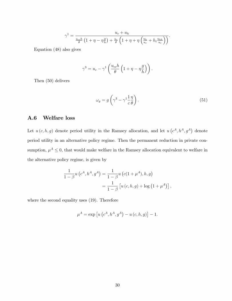
A.6 Welfare loss
Let u (c, h, g) denote period utility in the Ramsey allocation, and let u(cA, hA, gA
)denote
period utility in an alternative policy regime. Then the permanent reduction in private con-
sumption, µA ≤ 0, that would make welfare in the Ramsey allocation equivalent to welfare in
the alternative policy regime, is given by
1
1− βu(cA, hA, gA
)=
1
1− βu(c(1 + µA), h, g
)=
1
1− β[u (c, h, g) + log
(1 + µA
)],
where the second equality uses (19). Therefore
µA = exp[u(cA, hA, gA
)− u (c, h, g)
]− 1.
30

A.7 Conservative monetary-reaction function
The Lagrangian of the conservative monetary authority’s problem (20) is
max{ct+j ,ht+j ,Πt+j ,Rt+j}
∞∑j=0
βj{
(1− α)u(ct+j, ht+j, gt+j)−α
2(Πt+j − 1)2
+ γ1t+j
[uct+j(Πt+j − 1)Πt+j −
uct+jht+jθ
(1 + η + η
(uht+juct+j
− gt+jht+j
))− βuct+j+1(Πt+j+1 − 1)Πt+j+1
]+ γ2
t+j
[uct+jRt+j
− βuct+j+1
Πt+j+1
]+γ3
t+j
[ht+j − ct+j −
θ
2(Πt+j − 1)2 − gt+j
]},
where ct+j, ht+j,Πt+j, Rt+j, and gt+j−1 are taken as given for j ≥ 1.
The first-order conditions with respect to ct, ht,Πt, and Rt, respectively, are
(1− α)uct + γ1t
(ucct(Πt − 1)Πt −
uccthtθ
(1 + η − η gt
ht
))+ γ2
t
ucctRt
− γ3t = 0 (52)
(1− α)uht − γ1t
uctθ
(1 + η + η
uhtuct
+ ηhtuhhtuct
)+ γ3
t = 0 (53)
γ1t uct(2Πt − 1)− γ3
t θ(Πt − 1)− α (Πt − 1) = 0 (54)
−γ2t
uctR2t
= 0. (55)
Conditions (55), uct > 0, and Rt ≥ 1 imply
γ2t = 0.
Next, (52), (53), and (54), respectively, give
γ3t = (1− α)uct + γ1
t
(ucct(Πt − 1)Πt −
uccthtθ
(1 + η − η gt
ht
))(56)
γ3t = − (1− α)uht + γ1
t
uctθ
(1 + η + η
(uhtuct
+ htuhhtuct
))(57)
γ3t = γ1
t
uct(2Πt − 1)
θ(Πt − 1)− α
θ. (58)
Then (56) and (58) imply
31
γ1t =
θ(
1− α + 1uct
αθ
)2Πt−1Πt−1
− ucctuct
(θ(Πt − 1)Πt − ht
(1 + η − η gt
ht
)) . (59)
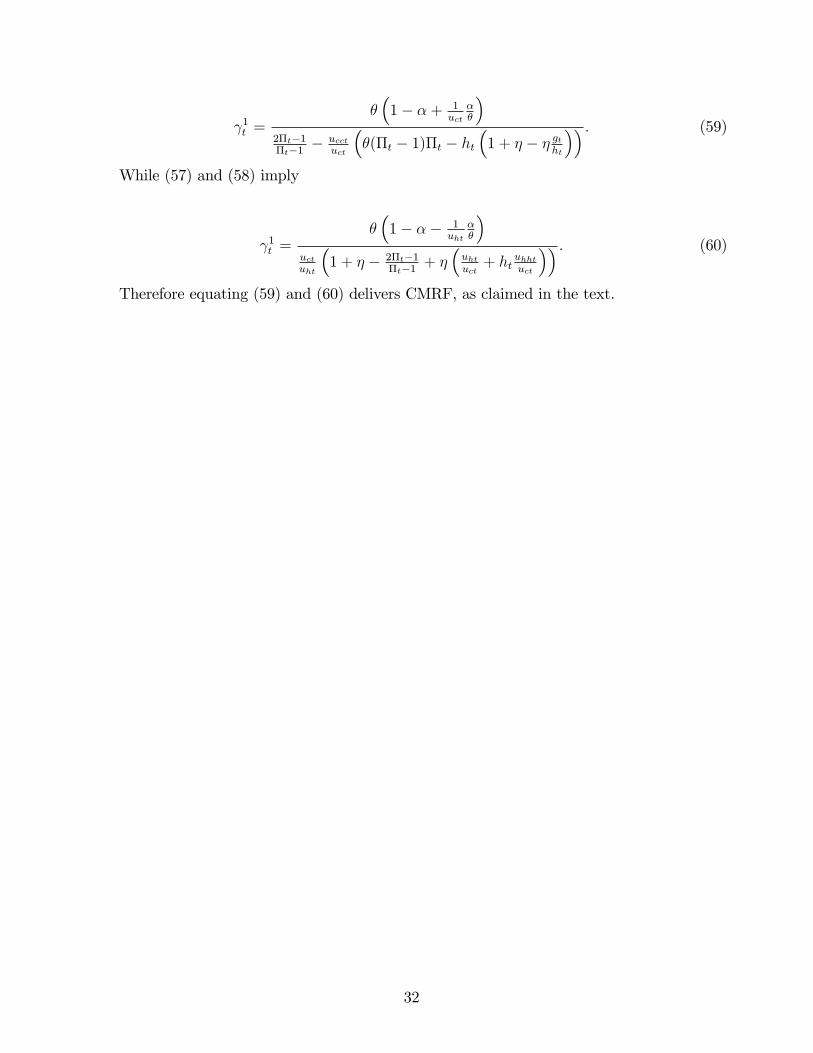
While (57) and (58) imply
γ1t =
θ(
1− α− 1uht
αθ
)uctuht
(1 + η − 2Πt−1
Πt−1+ η
(uhtuct
+ htuhhtuct
)) . (60)
Therefore equating (59) and (60) delivers CMRF, as claimed in the text.
32

Definition Parameter Value
Discount factor β 0.9913 quarterly
Price elasticity of demand η −6
Degree of price stickiness θ 17.5
Labor-supply elasticity ϕ−1 1
Labor-income tax rate τ 24%
Utility weight on labor effort ωh 19.7917
Utility weight on public goods ωg 0.2656
Table 1: Baseline calibration
33
Policy regime c h Π g τ Welfare loss
Difference from Ramsey (%) Level (%) Difference from Ramsey (%)
SP −7.08 5.90 4.47 14.21 25.71 −8.26
OI −13.73 −0.05 2.11 44.89 34.67 −4.76
Notes: Using the baseline calibration, the table shows the effects in steady state of sequential
monetary and fiscal policy (SP), and of an optimal-inflation (OI) regime in which monetary
policy is committed in advance. Shown are the effects on private consumption c, hours
worked h, gross inflation Π, public goods g, the labor-income tax rate τ , and the welfare
loss as measured by the permanent loss in private consumption.
Table 2: Effects of sequential policy
34
Calibration ΠSP − ΠOI Welfare loss
(%) Difference from Ramsey (%)
SP OI
Baseline 2.36 −8.26 −4.76
Stickier prices (θ = 50) 2.04 −11.70 −5.92
Less sticky prices (θ = 5) 2.13 −4.20 −2.94
Almost flexible prices (θ = 0.1) 0.15 −0.13 −0.13
Less competition (η = −5) 2.61 −11.90 −7.56
More competition (η = −9) 1.31 −3.28 −1.92
Almost perfect competition (η = −30) 0.06 −0.16 −0.15
High labor-supply elasticity (ϕ = 0.1) 3.27 −11.60 −6.89
Low labor-supply elasticity (ϕ = 3) 0.73 −3.14 −2.39
Almost inelastic labor supply (ϕ = 8) 0.07 −0.66 −0.62
Notes: See notes to table 2. The middle column shows the difference between gross
inflation in the SP regime and in the OI regime. A positive value of such difference
indicates inflation conservatism is desirable.
Table 3: Robustness of the effects of sequential policy
35

Calibration αopt Welfare loss
Difference from Ramsey (%)
Nash ML Nash and ML
α = αopt α = 1
Baseline 0.995 0.997 −4.76 −7.96
Stickier prices (θ = 50) 0.999 0.999 −5.92 −7.96
Less sticky prices (θ = 5) 0.963 0.982 −2.94 −7.96
Almost flexible prices (θ = 0.1) 0.015 0.300 −0.13 −7.96
Less competition (η = −5) 0.995 0.996 −7.56 −13.71
More competition (η = −9) 0.993 0.996 −1.92 −3.76
Almost perfect competition (η = −30) 0.939 0.991 −0.15 −1.40
High labor-supply elasticity (ϕ = 0.1) 0.996 0.996 −6.89 −10.94
Low labor-supply elasticity (ϕ = 3) 0.987 0.996 −2.39 −6.52
Almost inelastic labor supply (ϕ = 8) 0.925 0.993 −0.62 −5.83
Notes: See notes to table 2. The middle column shows the optimal degree of inflation
conservatism that in the Nash and monetary leadership (ML) regimes recovers the
level of welfare of the OI regime.
Table 4: Robustness of the welfare gain from inflation conservatism
36
0 0.1 0.2 0.3 0.4 0.5 0.6 0.7 0.8 0.9 110
9
8
7
6
5
4
3
2
1
0Welfare loss
Conservatism (α)
Diff
eren
ce fr
om R
amse
y (%
)
OICSPFLCSPMLCSPNash
Figure 1: Welfare gain from inflation conservatism under the baseline calibration
37

0 0.2 0.4 0.6 0.8 1
20
15
10
5
0Private consumption
Diff
eren
ce fr
om R
amse
y (%
)
Conservatism ( α)0 0.2 0.4 0.6 0.8 1
2
0
2
4
Hours worked
Diff
eren
ce fr
om R
amse
y (%
)
Conservatism ( α)
0 0.2 0.4 0.6 0.8 10
1
2
3
4
Gross inflation
Conservatism ( α)
Diff
eren
ce fr
om R
amse
y (%
)
OICSPFLCSPMLCSPNash
0 0.2 0.4 0.6 0.8 10
10
20
30
40
50
60
70
Public goods
Diff
eren
ce fr
om R
amse
y (%
)
Conservatism ( α)
Figure 2: Effects of inflation conservatism under the baseline calibration
38