1

Distributed active sonar detection in correlatedK-distributed clutter

Douglas A. Abraham

CausaSci LLCP.O. Box 5892

Arlington, VA 22205

Published in IEEE Journal of Oceanic EngineeringVol. 34, no. 3, pp. 343–357, July 2009

Abstract— Distributed active sonar systems exploit the simul-taneous detection of targets on multiple receiver platforms toimprove system performance. False alarm performance modelingfor such systems typically assumes independence from sensorto sensor; however, false alarms from clutter (e.g., shipwrecks,mud volcanoes, or rock outcroppings) are expected to producecorrelated data. In this paper, a clutter model exhibiting inter-sensor correlation and having K-distributed marginal probabilitydensity functions is proposed and analyzed. Under the constraintof equal sensor-level performance, the m-of-n fusion processorwas seen to be optimal for most cases of interest for all but theheaviest-tailed clutter. The system-level probability of false alarmis derived for the m-of-n fusion processor and approximationsare developed for the system-level probability of detection forcommon target models. In analyzing fusion performance, theAND processor (m = n) was seen to perform best in heavyclutter when the target model had some measure of inter-sensorconsistency while m/n ≈ 0.25 was seen to perform best for thehighly-variable Gaussian target model. The importance of ac-counting for inter-sensor correlation in false alarm performancemodeling was illustrated by an up to 10 dB over-estimation ofperformance when the clutter data are incorrectly assumed tobe independent.

Index Terms— active sonar, distributed detection, clutter, Kdistribution, data fusion

I. INTRODUCTION

Compared with a monostatic sonar system, the use ofdistributed sensing in active sonar can increase area coverage,improve detection performance, and refine localization byobtaining multiple, diverse observations of the target [1], [2],[3]. Distributed active sonar systems are typically designedso that a target is simultaneously detected on multiple sensors(despite variability in bistatic target strength [4] [5]) which canlead to improved localization and classification performance.However, false alarms arising from target-like clutter (e.g.,shipwrecks, rock outcrops, or mud volcanoes [6], [7]) are alsoexpected to be detected on multiple sensors. In this papera statistical model is proposed to represent such spatially-correlated clutter and evaluated in the context of distributed

Manuscript received April 28, 2008; revised August 15, 2008 and February05, 2009; accepted March 13, 2009. First published August 05, 2009. Thiswork was supported by the U.S. Office of Naval Research (Code 321MS)and the Naval Undersea Warfare Center Division Newport under ContractN66604-07-C-4452. Associate Editor: D. Knobles.

detection where the data from individual sensors are fused todecide if a target is present or not.

Communications constraints and a desire for robustness tomismatch often dictate the use of a two-tiered detection net-work topology where only binary decisions from the individualsensors are used to form the system-level decision [8], [9].The simplest analysis of this type of decentralized hypothesistesting involves modeling the data from multiple sensors asstatistically independent which leads to the application of alikelihood-ratio detector at each individual sensor [8]. Thesensor-level thresholds are chosen to optimize the system-levelperformance and are, in general, interdependent. However,under the assumption of equal performance at each sensor,separately for both the clutter-only and clutter-plus-targethypotheses (respectively, the null and alternative hypotheses),the optimal fusion rule is to decide a target is present whenat least m of the n sensors individually detect the target [10].The so-called m-of-n processor also arises in the processingof multiple radar sub-pulses [11] where it is known as binaryintegration or double-threshold detection. Specific cases ofthe m-of-n processor include the AND fusion rule (m = n)requiring all n sensors to detect the target for a system-leveldetection to occur and the OR fusion rule (m = 1) where onlyone sensor must detect the target.

Analysis of the m-of-n fusion rule has not been com-pletely restricted to independent sensor data. For example,both correlated signals [12] and correlated noise [13], [14]have been considered, although there do not appear to beany general analytical results. An interesting finding from[13] for a constant target in additive, correlated Gaussian orLaplacian noise was a degradation in detection performanceas the inter-sensor noise correlation increased. Similarly, thebulk of distributed-detection analysis has been performed forGaussian data (or equivalently for Gaussian-derived processessuch as Rayleigh-distributed envelope data). In addition to theexamination of Laplacian noise in [13], other non-Gaussian-derived distributions considered include the Weibull and Kenvelope distributions in [15] and a generalized Gaussian dis-tribution in [10] and [16]. However, with the exception of [13],each assumed independence from sensor to sensor. Notingthat the m-of-n processor can be analyzed by considering theorder statistics of the sensor-level detection statistics prior to

2

thresholding, the limited analysis for correlated data is mostlikely attributable to the general difficulty in analyzing theorder statistics of correlated data [17]

The focus of this paper is on evaluating the performance ofthe m-of-n fusion processor in the presence of K-distributed[18] clutter having inter-sensor dependence. In Section II, amodel amenable to such analysis and having K-distributedmarginal probability density functions (PDFs) is proposedand examined for representing correlated active sonar clutterechoes. The optimality of the m-of-n fusion processor isconsidered for this clutter model in Section III as well asderiving exact or approximate formulae for the system-levelfalse alarm and detection probabilities for non-fluctuating(herein referred to as Type 0) and Swerling Type I and IItarget models. Section IV examines the performance gainachieved by fusion in the presence of correlated K-distributedclutter, the effect of varying the clutter PDF tails, the optimalvalue of m in the m-of-n processor, and the error involvedin incorrectly assuming inter-sensor clutter independence insonar performance prediction.

II. MODELING OF CORRELATED ACTIVE SONAR CLUTTER

In a distributed active sonar system, a single-ping, system-level detection decision is typically made by combining datafrom range-bearing cells at each receiver pointing to the samegeographic position (accounting for localization errors [19]).This is usually done in the context of centralized tracking[20], [21] with the sensor-level data as either the normalizedmatched filter intensity for the spatially overlapping range-bearing cells or, under severe communication constraints,binary sensor-level detection decisions. The majority of anal-ysis of such systems assumes the sensor-level data to bestatistically independent. Although this might be appropriatefor false alarms from random threshold crossings arising fromspatially homogenous processes such as diffuse reverberationor ambient noise, it is not expected to be accurate for falsealarms arising from target-like echoes commonly called clutterin sonar (akin to clutter-discretes in radar), which can bea limiting factor in sonar system performance. Owing tothe spatially compactness of many types of clutter sources(e.g., shipwrecks, mud volcanoes, rock outcroppings, etc.) theechoes measured at multiple sonar receivers are more likelyto be correlated than statistically independent.

A similar situation occurs when fusing the data at a singlesonar receiver from sub-pulses within a single-ping wavetrain[22] or from multiple consecutive pings (e.g., as in a track-before-detect scheme or tracklet formation in distributed track-ing [23], [20]). The temporal stationarity of the ocean overshort time periods leads to an expectation of correlated multi-ping or sub-pulse data. A similar assumption is made in thederivation of the Swerling Type I target model (see for examplethe discussion in [11, Sect. 9.2]) where the amplitude is takenas constant over several closely-spaced observations (e.g.,waveform sub-pulses), but then changes randomly over longertimes (from scan to scan). The viability of synthetic aperturesonar processing for low-frequency active sonar systems [24]and reverberation nulling using time-reversal [25] support this

assumption for active sonar clutter as both require coherenceor correlation between echoes on multiple, consecutive pings.The argument is weaker for distributed systems where sen-sors might receive echoes from different aspects. However,some correlation is still expected for spatially-compact clut-ter sources having azimuthally isotropic or broad scatteringpatterns.

Although the focus of this paper is on the detection per-formance of a distributed system when fusing data from asingle ping, many of the concepts, results, and analysis areapplicable to the alternative example of fusing active sonardata over multiple pings at a single receiver.

A. A real-data example

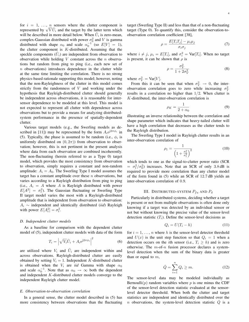
As an example of what correlation might be observedbetween clutter echoes, a preliminary analysis of data obtainedfrom the NATO Undersea Research Centre’s Clutter 2007experiment (please see the acknowledgments in Sect. VI)is presented in Fig. 1. The Clutter 2007 experiment tookplace in the Malta Plateau area of the Mediterranean Seafrom early May to early June of 2007. The data presentedin Fig. 1 were obtained from circular tracks 2 km distantfrom a shipwreck at 36◦ 18.804′ N by 14◦ 44.136′ E on May12, 2007 and around a mud volcano field about the point36◦ 34.218′ N by 14◦ 25.878′ E on May 21, 2007. A 0.5-s linear frequency modulated (LFM) waveform from 800–1800 Hz was transmitted every 12 s yielding a sampling of theclutter-source echoes at an aspect resolution of less than onedegree. After matched filtering and beamforming, the clutterecho on each ping was isolated by manually choosing thebeam with the highest signal-to-noise power ratio (SNR) andthen through the use of Page’s test as described in [26] tofind the echo start and stop times. The maximum correlationcoefficient (see eq. (7) in Sect. II-E) between the intensitysignals on each pair of echoes is computed. The averageof all samples with aspect separation within 0.5 degrees ofeach unit degree from (−180, 179) is then plotted in Fig. 1.As seen in the figure, the shipwreck and mud volcano fieldshow a correlation coefficient between 0.4 and 0.5 with largervalues at the lower aspect separations and a slow fall offas the aspect separation grows. For comparison, a SwerlingType I target and independent Rayleigh and K-distributed(shape parameter α0 = 1) clutter were simulated with an echoduration of 200 independent samples (approximately the sameas the real data) and subjected to the same processing. Asderived in Sect. II-E, the Swerling Type I target with an SNRof 12.7 dB is expected to yield a correlation coefficient of 0.9.Although the independent clutter data should result in zerocorrelation, the process of choosing the maximum results ina biased estimate—it is therefore expected that the real dataresults are similarly biased high. However, clutter echoes fromdifferent aspects arising from the same source transmissionmight be expected to have a higher correlation than thosearising from multiple monostatic transmission as is the casewith these data. Note that at 0◦ aspect separation in the figure,the real data contain some values ∈ (−0.5◦, 0.5◦) that werenot equal to zero (the simulated data were all at 0◦ separation)

3

and therefore did not have a unit correlation coefficient, whichcauses the reduced average value seen in the figure. The datain Fig. 1 present some initial evidence of correlation for clutterechoes in a distributed active sonar system. A more detailedanalysis of the measurements is currently underway.

Fig. 1. Estimated correlation in matched-filter intensity as a function ofaspect separation for various simulated data (independent Rayleigh- and K-distributed clutter and a Swerling Type I target) and real data (a shipwreckand a mud-volcano field). The estimates are averaged over each unit degreeof aspect separation. Despite the high bias seen in the simulated clutter data,the real data exhibit non-zero correlation.

B. The K distribution

Both empirical evidence [27], [28], [7] and theoretical mod-els [18], [29], [27], [30] support the use of the K distribution[18] to model the statistical fluctuations of clutter echoes.The K-distribution PDF and cumulative distribution function(CDF) are [31]

fK (t;α0, λ0) =2

λ0Γ(α0)

(t

λ0

)α0−12

Kα0−1

(2√

t

λ0

)(1)

and

FK (t;α0, λ0) = 1− 2Γ(α0)

(t

λ0

)α02

Kα0

(2√

t

λ0

)(2)

where t ≥ 0 is the matched filter intensity, α0 is the shapeparameter and λ0 is a scale parameter. The shape parametercontrols the tails of the PDF with large values producingRayleigh-like envelope data and small values yielding heavy-tailed clutter.

Of the theoretical models resulting in the K distribution, theproduct form [30] is exploited in this paper to derive a modelfor correlated active sonar clutter echoes. The product form ofthe K distribution describes the matched filter intensity as theproduct

T = V U (3)

where V is gamma distributed with shape parameter α0

and scale parameter 1/α0 and U is exponentially distributedwith mean σ2

0 = α0λ0 and independent of V . In the radar

sea-surface clutter community, U is the speckle componentrepresentative of Rayleigh backscattering (i.e.,

√U is Rayleigh

distributed) and V is a modulation induced by wave motionwith empirical evidence supporting it following the gammadistribution.

C. A model for spatial dependence

In general, correlated samples can be difficult to analyzeowing to the need for a joint probability density functionover all the variables. Typically, the multivariate Gaussiandistribution is invoked in representing correlated data owing tothe simplicity of decorrelating the data and the tractability ofanalysis after the data are whitened. In developing a modelrepresenting correlated active sonar clutter, the need for atractable analysis must be balanced with the desire for anaccurate representation of the scattering physics. As mentionedin the previous section, a model having the K distribution asthe univariate marginal PDF is supported by both empiricalanalysis and theoretical models. The theoretical models witha physical basis [29], [27] do not readily lend themselves to amultiple-observation model with a tractable analysis. However,the product form of the K-distribution [30] does. Given nobservations of a clutter source with each being marginally K-distributed, the matched filter intensity of the ith observationwould have the form

Ti = ViUi (4)

where Vi and Ui are independent and, respectively, gammaand exponentially distributed as described in Sect. II-B. Thismodel has been used in the radar community [32], [33], [34] torepresent spatially-correlated clutter; however, the correlationis in short time (contiguous delay cells on a given beam andping) rather than across sensors or pings. In [32] and [33]correlation is induced by making each modulation pair (Vi, Vj)dependent while in [34] each pair of speckle components(Ui, Uj) is additionally made correlated.

A more appropriate model might be found from [35] wheredata from multi-look synthetic aperture radar (SAR) weremodeled as K-distributed where Vi was held constant for alli and the speckle components (Ui, Uj) were correlated. Atthe complex matched filter envelope stage, such a model isidentical to the spherically invariant random vector (SIRV)models which have seen significant use in the radar community[36] and been exploited in the sonar community [37] torepresent data in the neighborhood of a test cell across delayand beam. Unfortunately, when applied to fusing the data frommultiple observations, these more general dependent cluttermodels are typically not easy or at times even possible toanalyze.

A further simplification to the statistical model describedby (4) is required to enable analysis of the m-of-n fusionprocessor. Following [35], let Vi be constant over all obser-vations, but let the pair (Ui, Uj) be independent for i 6= j.The sensor-level detection statistic, including an additive targetcomponent, would have the form

Ti =∣∣∣√V Ui +Aiej2πφi

∣∣∣2 (5)

4

for i = 1, . . . , n sensors where the clutter component isrepresented by

√V Ui and the target by the latter term which

will be described in more detail below. When Ui is zero-mean,complex-Gaussian distributed with power σ2

0 and V is gammadistributed with shape α0 and scale α−1

0 (so E[V ] = 1),the clutter component is K-distributed. Assuming that thespeckle components (Ui) are independent from observation toobservation while holding V constant across the n observa-tions but random from ping to ping (i.e., each new set ofn observations) introduces dependence in the clutter whileat the same time limiting the correlation. There is no strongphysics-based rationale supporting this model; however, notingthat the non-Rayleighness of the clutter in this model comesstrictly from the randomness of V and working under thehypothesis that Rayleigh-distributed clutter should generallybe independent across observations, it is reasonable for inter-sensor dependence to be modeled at this level. This model isnot expected to represent all clutter with dependence acrossobservations but to provide a means for analyzing distributed-system performance in the presence of spatially-dependentclutter.

Various target models (e.g., the Swerling models as de-scribed in [11]) may be represented by the form Aiej2πφi in(5). Typically, the phase is assumed to be random (i.e., φi isuniformly distributed on (0, 2π)) from observation to obser-vation; however, this is not pertinent in the present analysiswhere data from each observation are combined incoherently.The non-fluctuating (herein referred to as a Type 0) targetmodel, which provides the most consistency from observationto observation, simply requires a constant and non-randomamplitude: Ai = A0. The Swerling Type I model assumes thetarget has a constant amplitude over these n observations, butvaries according to a Rayleigh distribution from ping to ping(i.e., Ai = A where A is Rayleigh distributed with powerE[A2] = σ2

t ). The Gaussian fluctuating or Swerling TypeII target model varies the most with a Rayleigh-distributedamplitude that is independent from observation to observation:Ai ∼ independent and identically distributed (iid) Rayleighwith power E[A2

i ] = σ2t .

D. Independent clutter models

As a baseline for comparison with the dependent cluttermodel of (5), independent clutter models with data of the form

Ti =∣∣∣√ViUi +Aiej2πφi

∣∣∣2 (6)

are utilized where Vi and Ui are independent within andacross observations. Rayleigh-distributed clutter are easilyobtained by setting Vi = 1. Independent K-distributed clutteris obtained when the Vi are iid Gamma with shape α0

and scale α−10 . Note that as α0 → ∞ both the dependent

and independent K-distributed clutter models converge to theindependent Rayleigh clutter model.

E. Observation-to-observation correlation

In a general sense, the clutter model described in (5) hasmore consistency between observations than the fluctuating

target (Swerling Type II) and less than that of a non-fluctuatingtarget (Type 0). To quantify this, consider the observation-to-observation correlation coefficient [38],

ρ =E[TiTj ]− µiµj

σiσj(7)

where i 6= j, µi = E[Ti], and σ2i = Var[Ti]. When no target

is present, it can be shown that ρ is

ρ =σ2V

1 + 2σ2V

(8)

where σ2V = Var[V ].

From this it can be seen that when σ2V → 0, the inter-

observation correlation goes to zero while increasing σ2V

results in a correlation no higher than 1/2. When clutter isK-distributed, the inter-observation correlation is

ρK =1

2 + α0(9)

illustrating an inverse relationship between the correlation andshape parameter which indicates that heavy-tailed clutter willhave a high correlation that decreases as the clutter tends tothe Rayleigh distribution.

The Swerling Type I model in Rayleigh clutter results in aninter-observation correlation of

ρ1 =1(

1 + σ20σ2t

)2 (10)

which tends to one as the signal-to-clutter power ratio (SCR= σ2

t /σ20) increases. Note that an SCR of only 3.8 dB is

required to provide more correlation than any clutter modelof the form found in (5) while an SCR of 12.7 dB yields aninter-observation correlation of 0.9.

III. DISTRIBUTED-SYSTEM Pfa AND Pd

Particularly in distributed systems, deciding whether a targetis present or not from multiple observations is often done onlyknowing if a target was detected by an individual sensor ornot but without knowing the precise value of the sensor-leveldetection statistic (Ti). Define the sensor-level decisions as

Qi = U(Ti − h) (11)

for i = 1, . . . , n where h is the sensor-level detector thresholdand U(x) is the unit step function so that Qi = 1 when adetection occurs on the ith sensor (i.e., Ti ≥ h) and is zerootherwise. The m-of-n fusion processor declares a system-level detection when the sum of the binary data is greaterthan or equal to m,

Q =n∑i=1

Qi ≥ m. (12)

The sensor-level data may be modeled individually asBernoulli(p) random variables where p is one minus the CDFof the sensor-level detection statistic evaluated at the sensor-level detector threshold. When both the clutter and targetstatistics are independent and identically distributed over then observations, the system-level detection statistic Q is a

5

binomial(n, p) random variable. Therefore, from [11, Sect.9.8], the system-level exceedance distribution function (EDF)is

Pe(Hj) = Pr{Q ≥ m |Hj

}= 1−

m−1∑i=0

(n

i

)Fn−iT (h;Hj) [1− FT (h;Hj)]

i (13)

from which Pfa is obtained under the clutter-only hypothesis(H0) and Pd under the clutter-plus-target hypothesis (H1). In(13) FT (t;Hj) is the CDF of Ti under hypothesis Hj .

Dependent clutter and the Swerling Type I target modelclearly violate the above assumptions. However, owing to thecommonality of V in the clutter component in (5) across allsensors, Pfa and some Pd analysis are feasible for the m-of-n fusion processor. In the following sections, conditionsfor the optimality of the m-of-n processor in dependent K-distributed clutter are described, an analytical result for thesystem-level Pfa is derived, and then approximations andnumerical evaluations of Pd for the various target models arepresented.

A. Optimality of m-of-n fusion in spatially-correlated clutterIn [10], Reibman and Nolte showed that under a restricted

scenario where the sensor-level data are statistically indepen-dent with constant Pd and Pfa across all sensors, the m-of-n fusion processor implements the likelihood ratio of binarydata describing sensor-level alarms and is therefore optimal.Unfortunately, the result does not universally extend to thedependent clutter model described in (5). However, it will beshown that the m-of-n processor is optimal for many cases ofinterest.

Conditioning on V in (5) results in independent sensor dataunder H0 and under H1 for the Type 0 and Swerling TypeII targets. Extension to the Swerling Type I target will bedescribed at the end of the section. Define the sensor-levelPd and Pfa conditioned on V as pd(V ) and pfa(V ) wherethe lower-case p denotes sensor-level probabilities rather thangeneric or system-level. These sensor-level conditional detec-tion measures are simply derived from the standard sonar/radarmodels. For example, conditioned on V under H0, Ti isexponentially distributed with mean V σ2

0 so

pfa(v) = e− h

vσ20 . (14)

Similarly, the Swerling Type II target model results in Ti beingconditionally exponentially distributed with mean V σ2

0 + σ2t

sopd(v) = e

− h

vσ20+σ2t . (15)

The Type 0 target will result in Ti conditionally being the scaleof a non-central chi-squared random variable with two degreesof freedom (or the square of a Rician-distributed envelope),yielding

pd(v) = 1− Fχ22,δ

(2hvσ2

0

)(16)

where Fχ2ν,δ

(x) is the CDF of the non-central chi-squareddistribution with ν degrees of freedom and non-centralityparameter δ, which is a function of v in (16), δ = 2A2

0/(vσ20).

Conditioned on V , the sensor-level decisions Q1, . . . , Qnare iid Bernoulli random variables with probability pfa(V )under H0 and pd(V ) under H1. The joint likelihood functionof the sensor-level binary decisions is then easily obtainedfrom that for iid Bernoulli data followed by an expectationremoving the conditioning on V yielding

f1(q) =∫ ∞

0

pd(v)q [1− pd(v)]n−q fV (v) dv (17)

under H1 and

f0(q) =∫ ∞

0

pfa(v)q [1− pfa(v)]n−q fV (v) dv (18)

under H0 where fV (v) is the PDF of V , q = [q1 · · · qn],and q =

∑ni=1 qi. Noting that q is a sufficient statistic, the

likelihood ratio, when described as a function of q, is

l(q) =f1(q)f0(q)

=

∫∞0pd(v)q [1− pd(v)]n−q fV (v) dv∫∞

0pfa(v)q [1− pfa(v)]n−q fV (v) dv

.

(19)If l(q) is monotonically increasing with q, then comparing Qto a threshold (as is done in the m-of-n fusion processor)implements the likelihood ratio test on the binary sensor-leveldetection data and provides the highest system-level Pd for afixed Pfa1.

Unfortunately, l(q) is not necessarily monotonic for allclutter and target distributions resulting in data of the formfound in (5) and therefore the likelihood ratio of (19). Someindication of when it is comes from the following analysis.First (19) is described as a ratio of expectations

l(q) =E [gd(V, q)]E [gfa(U, q)]

(20)

where V and U are iid random variables with PDF fV (v),

gd(v, q) = pd(v)q [1− pd(v)]n−q (21)

andgfa(v, q) = pf (v)q [1− pf (v)]n−q . (22)

The likelihood ratio is then monotonically increasing in q ifit can be shown that l(q) < l(q + 1) or, equivalently,

E [gd(V, q)]E [gfa(U, q)]

<E [gd(V, q + 1)]E [gfa(U, q + 1)]

(23)

for q = 0, . . . , n − 1. Cross-multiplying in (23), subtractingby the right-hand side, and collating the arguments of theexpectations under one expectation over both V and U resultsin the need to show that I < 0 where

I = E [gd(V, q)gfa(U, q + 1)− gd(V, q + 1)gfa(U, q)] .(24)

By exploiting the mean-value theorem for double integrals [40]extended to apply to expectations (e.g., see [41, Sect. 12.111]for the univariate case), a point (u0, v0) ∈ <+2, where <+ =[0,∞), can be found such that

I = gd(v0, q)gfa(u0, q + 1)− gd(v0, q + 1)gfa(u0, q). (25)

1Owing to the discrete nature of Q, a randomized test [39] might berequired to achieve certain values of Pfa.

6

It is then straightforward to show that I < 0 when

pfa(u0) < pd(v0). (26)

Note that the pair (u0, v0) will depend on q, so (26) must holdfor all q = 0, . . . , n− 1.

Recalling that E[V ] = E[U ] = 1, it is reasonable to expectthat u0 and v0 are near one, with less deviation when σ2

v

is small, which represents the case of near-Rayleigh clutterand weak inter-sensor correlation. Noting that pd(v) > pf (v)for all v for any non-zero additive signal, and that pd(v) andpf (v) are increasing functions with v implies that (26) willbe satisfied whenever u0 < v0. Additionally, when the SCRis high enough to result in pd(1) � pf (1) (most cases ofinterest), the monotonicity will likely persist for many valuesof u0 > v0. However, when the PDF of V has significantweight at high values, u0 might be too large resulting in anon-monotonic l(q).

A numerical analysis of the monotonicity of the likelihoodratio with q for correlated, K-distributed clutter and the Type 0and Swerling Type II targets confirmed the expectation that in-creasing SCR and decreasing clutter tail heaviness encouragesmonotonicity and also identified a dependence on n where ifl(q) is monotonic for a given n it is also monotonic for smallervalues of n—perhaps arising from a greater reduction in v0

than u0 as n increases. The results of the numerical analysisare therefore shown in Fig. 2 as the maximum value of nfor which l(q) is monotonic as a function of α0 for variousvalues of SCR, the Type 0 and Swerling Type II targets, anda sensor-level Pfa = 10−4. The likelihood ratio for the Type0 target is seen to exhibit monotonicity at very low valuesof SCR (≤ 5 dB) in the presence of very heavy-tailed clutter(α0 ≤ 1) for moderate values of n. The sensor-level Pd forthe Type 0 target was less than 10−3, even for the largest SCR(5 dB) and lightest clutter tails (α0 = 1) shown in the figure.The Swerling Type II target likelihood ratio required a higherlevel of SCR for monotonicity in the heavy-tailed clutter; forthe 15 dB SCR case, the sensor-level Pd was 0.27 at α0 = 0.5and 0.42 at α0 = 1. However, differing from the Type 0 target,the likelihood ratio was always found to be monotonic whenα0 > 1. Lowering the sensor-level Pfa shifted the curvesfor the Type 0 target to the left and the Swerling Type IItarget to the lower right (respecting the vertical asypmtoteat α0 = 1), while increasing the sensor-level Pfa had theopposite effect. Thus, the m-of-n processor is foreseeablythe optimal processor for correlated, K-distributed clutter inmost situations of interest, with some counter examples in thecombination of very heavy-tailed clutter, large n, and SCR nothigh enough for moderate sensor-level Pd.

The above analysis may be extended to account for aSwerling Type I target or, more generally, any target with arandom amplitude that is constant over all sensors. This isaccomplished by including the random target amplitude (A)in the expectation in the numerator of (20). The inequalityproviding monotonicity then becomes

pfa(u0) < pd(v0, a0) (27)

where a0 is obtained from the mean-value theorem. Similarresults to those reported for the Type 0 and Swerling Type II

Fig. 2. Maximum value of n for which the likelihood ratio is monotonic inq indicating the optimality of the m-of-n processor. Note that when α0 > 1,the m-of-n processor is optimal for all n for the Swerling Type II targets andincreasingly large n for the Type 0 target.

targets are expected for the Swerling Type I target.

B. Pfa analysis

As previously mentioned, the most common analysis of them-of-n fusion rule follows from characterizing the sensor-level data as being iid Bernoulli random variables. Alterna-tively, the detection statistic can be taken as the (n−m+ 1)storder statistic of the sensor data {T1, . . . , Tn}. Let the ordereddetection statistics be

T(1) ≤ T(2) ≤ · · ·T(n). (28)

Thus if T(n−m+1) exceeds the sensor-level detection threshold,then at least m of the n samples exceed that threshold. Thoughthe two implementations of the m-of-n fusion processor areidentical in terms of their statistical performance, the order-statistic-based implementation is less preferable in practice asit requires access to the detection statistic from each sensorrather than the binary, single-sensor decision.

In general, it is difficult to analyze the ordered statisticsof correlated data [17]. However, by conditioning on V , thedata are independent under H0 and follow an exponentialdistribution for which previous results may be exploited todetermine the system-level Pfa of the dependent clutter modelin (5). Conditioned on V under H0, the sensor-level detectionstatistics {T1, . . . , Tn} are iid exponential random variableswith mean λ = V σ2

0 . The (n −m + 1)st order statistic maybe described as

T(n−m+1) =n−m+1∑i=1

∆i (29)

where ∆i is the difference between the ith and (i−1)st orderstatistics (i.e., ∆i = T(i) − T(i−1)) with ∆1 = T(1). From[42, Chapt. I.6], when the data are iid exponential randomvariables with mean λ, ∆1, . . . , ∆n are independent and

7

exponentially distributed with mean E [∆i] = λ/(n− i + 1).The characteristic function of T(n−m+1) may then be formedas the product of the characteristic functions of the ∆i andsimplified to

Φ(ω) =n−m+1∏i=1

(1− jωλ

n− i+ 1

)−1

(30)

=n−m+1∑i=1

bn−i+1

(1− jωλ

n− i+ 1

)−1

(31)

where the summation in (31) is obtained through partialfraction expansion which yields the coefficients

bi =n∏

l=m, 6=i

(1− i

l

)−1

. (32)

The PDF of T(n−m+1) conditioned on V is then easily seento be

f0(t|V ) =n∑

i=m

bi(λ/i)

e−t/(λ/i) (33)

which is a mixture of exponential PDFs, each with meanλ/i = V σ2

0/i. Recalling that for K-distributed clutter dataconditioned on V , Ti is exponentially distributed with meanV σ2

0 , it is seen that each term in the sum of (33) will resultin a K-distributed intensity PDF (fK (t;α, λ) from (1)) whenthe conditioning on V is removed with the scale parameterscaled by i−1,

f0(t) = EV [f0(t|V )] =n∑

i=m

bifK

(t;α0,

σ20

iα0

); (34)

that is, the PDF of the (n − m + 1)st order statistic forthe dependent clutter model is a mixture of K-distributionPDFs. Integrating the PDF of the (n−m+ 1)st order statisticresults in the CDF which is a mixture of K-distribution CDFs(FK (t;α, λ) from (2)),

F0(t) =n∑

i=m

biFK

(t;α0,

σ20

iα0

). (35)

The system-level Pfa for the dependent clutter model of (5)is then easily obtained from (35) as

Pfa = 1− F0(h)

= 1−n∑

i=m

biFK

(h;α0,

σ20

iα0

)

=2

Γ(α0)

(hα0

σ20

)α02 n∑i=m

bi iα02 Kα0

(2σ0

√hiα0

)(36)

where h is the sensor-level detection threshold and the factthat

n∑i=m

bi = 1 (37)

has been exploited.

C. Extension of Pfa analysis to other clutter models

Owing to the form of (33), these results are not restricted toclutter following the K-distribution, but apply to any modelthat may be described as a common amplitude modulatingan iid Gaussian speckle component. For example, if theclutter envelope followed a Rayleigh-mixture distribution withprobability πl of observing power γl for l = 1,. . . ,L (whichyields average clutter intensity σ2

0 =∑Ll=1 πlγl), then the Pfa

is

Pfa =n∑

i=m

L∑l=1

biπle−hi/γl . (38)

Similarly, if the clutter intensity data are Weibull dis-tributed with shape parameter β and average intensity σ2

0 =ηΓ(1 + β−1

), then

Pfa =n∑

i=m

bie−(hi/η)β (39)

where β = 1 results in independent Rayleigh clutter.

D. Pd evaluation

In this section methods are provided for evaluating thesystem-level Pd for each of the target models being considered.Approximations are developed that enable Pd computationusing at most a one-dimensional numerical integral overstandard functions. The approximations are compared withsimulation results for a variety of scenarios to determine theirregion of validity. The values considered for each parameter inthe comparison are shown in Table I. For all cases considered,σ2

0 = 1 and the SCR is varied. For the Type 0 target model,SCR = A2

0/σ20 while for the Swerling Type I and II models

it is σ2t /σ

20 .

TABLE IPARAMETERS CONSIDERED IN COMPARISON OF Pd APPROXIMATIONS TO

SIMULATION.

Parameter Values evaluatedn 3, 7, and 11m 1, (n+ 1)/2, and nα0 1, 2, 10, and 100Pfa 10−2, 10−4, and 10−6

σ20 1

SCR various

1) Type 0 target: The Type 0 or non-fluctuating targetresults in sensor data (from (5) with Ai = A0)

Ti =∣∣∣√V Ui +A0ej2πφi

∣∣∣2 (40)

where the target amplitude A0 is deterministic (i.e., constantand known). As previously noted, Ti given V is the scale ofa non-central chi-squared random variable with two degreesof freedom. Thus, the system-level Pd can be described byinserting the non-central chi-squared CDF (Fχ2

2,δ(x)) into (13)

to obtain Pd for the m-of-n processor given V followed by

8

an expectation over V which removes the aforementionedconditioning, resulting in

Pd(h) = 1−∫ ∞

0

fV (v)× (41)

m−1∑i=0

(n

i

)Fn−iχ2

2,δ

(2hvσ2

0

)[1− Fχ2

2,δ

(2hvσ2

0

)]idv

where the non-centrality parameter δ = 2A20/(vσ2

0

)is a

function of v. As V is gamma distributed with unit mean andvariance 1/α0, it has PDF

fV (v) =αα0

0 vα0−1

Γ(α0)e−α0v (42)

and the integral can be limited to a region around one thatcollapses as α0 increases. The non-central chi-squared CDFis related to Marcum’s Q-function [43] and is itself describedby a one-dimensional integral or infinite summation. If asubroutine for evaluating Marcum’s Q function or the non-central chi-squared CDF is not available or if computationalcapability is limited, many approximations may be foundin [44] including Pearson’s shifted-gamma and Sankaran’spower-law-normal approximations. These approximations arefairly accurate except for low values of the CDF which essen-tially equates to low threshold values or high Pfa. Sankaran’smost flexible approximation is detailed in the Appendix andused in (41) in a comparison with simulation to determine itsaccuracy. An example of the results may be found in Figure3 for Pfa = 10−4, n = 7 and α0 = 1. A total of 5,000trials were used in the simulation. The average and maximumabsolute errors in SCR over all of the scenarios described inTable I for Pd ∈ [0.25, 0.95] are shown in Table II whereit can be seen that both are fractions of a decibel for theType 0 target. As might be expected from using Sankaran’sapproximation to the non-central chi-squared CDF, accuracywas worst for the highest Pfa and n and lowest m and SCR.

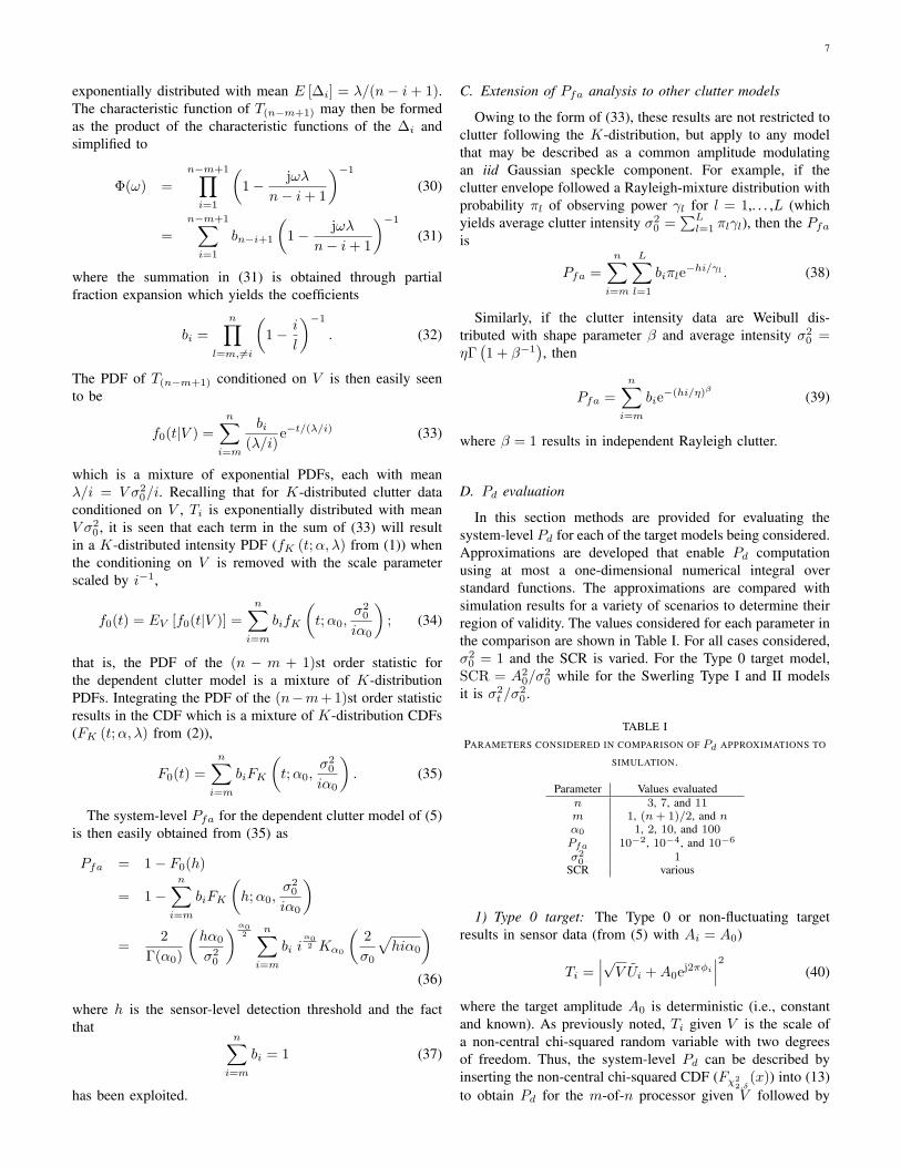
Fig. 3. Modeled and simulated Pd for the three target models for n = 7,m = 1, 4, and 7, Pfa = 10−4, and α0 = 1. The model results are solidlines while the simulated results are dashed.

TABLE IIAVERAGE AND MAXIMUM (LATTER IN PARENTHESES) ABSOLUTE ERROR

IN SCR (dB) BETWEEN MODEL AND SIMULATION OVER ALL CASES

CONSIDERED FOR EACH Pfa AND OVER THE RANGE Pd ∈ [0.25, 0.95].

Pfa Type 0 Swerling Type I Swerling Type II10−2 0.037 (0.18) 0.19 (0.95) 0.075 (0.45)10−4 0.027 (0.16) 0.14 (0.55) 0.055 (0.43)10−6 0.018 (0.099) 0.12 (0.57) 0.06 (0.48)

2) Swerling Type I target: The Swerling Type I target, asutilized here to represent target echoes received on multiplesensors in a distributed active sonar system, fluctuates ran-domly from ping to ping, but is constant within a ping resultingin sensor data (from (5) with Ai = A)

Ti =∣∣∣√V Ui +Aej2πφi

∣∣∣2 (43)

where the target amplitude A is a Rayleigh-distributed randomvariable with power E[A2] = σ2

t . The system-level Pd can bedetermined exactly by conditioning on both A and V , insertingthe non-central chi-squared CDF in (13), and then removingthe conditioning by a two-dimensional integral implementingthe expectation over A and V . However, an accurate andless computationally expensive approximation is obtained byassuming that the clutter envelope is Rayleigh distributed andindependent from sensor to sensor (i.e., let α0 →∞ or V = 1)resulting in

Pd(h) ≈ 1−∫ ∞

0

fA(a)m−1∑i=0

(n

i

)Fn−iχ2

2,δ

(2hσ2

0

)×[1− Fχ2

2,δ

(2hσ2

0

)]ida (44)

where δ = 2a2/σ20 and

fA(a) =2aσ2t

e−a2/σ2

t . (45)

Additional computational savings are obtained by usingSankaran’s approximation to the non-central chi-squared CDFas described in the previous section and the Appendix. Atthe expense of more complicated coding, the computationalburden could be reduced further through a technique describedby Walker [45] (which can be found in [46, Sect. 3.4]) wherethe region of integration over the target amplitude is limitedby exploiting the fact that the sum in (44) tends to one forlarge enough values of a.

The iid-Rayleigh-distributed clutter approximation subvertsone of the integrals and leads to significant computational sav-ings, yet surprisingly results in an accurate approximation, ascan be seen in Fig. 3 and Table II. Of the three target types, thisapproximation results in the highest average errors, althoughthey are still less than one fifth of a decibel. The worst casemaximum SCR error was just under one decibel and occurredfor the highest Pfa (owing to Sankaran’s approximation), thelowest α0 (owing to the Rayleigh clutter approximation), andthe highest n and m. As illustrated in Fig. 3, the approximationslightly underestimates performance for m = n but is quiteaccurate for lower values of m.

9

3) Swerling Type II target: The Swerling Type II targetprovides the most fluctuation of the three targets consideredwith independent random fluctuation from sensor to sensor.The sensor data are as in (5) with the A1, . . . , An iidRayleigh distributed with power σ2

t . The system-level Pd canbe determined exactly by conditioning on V , evaluating (13)with an exponential CDF with mean E[Ti|V ] = V σ2

0 + σ2t

followed by an integral removing the conditioning on V .However, as with the Swerling Type I target of the previoussection, an approximation assuming iid Rayleigh-distributedclutter provides an accurate and easily evaluated alternative,

Pd(h) ≈ 1−m−1∑i=0

(n

i

)[1− e−h/(σ

20+σ2

t )]n−i

e−hi/(σ20+σ2

t ).

(46)

As seen in Fig. 3 and Table II, the average absolute error inSCR is less than one tenth of a decibel for each Pfa and themaximum errors all less than half of a decibel.

It is surprising that assuming iid Rayleigh-distributed clutterleads to an accurate approximation for the Swerling Type Iand II target models while it fails to provide an accurateapproximation for a non-fluctuating target. Heuristically, itmight be assumed that at high SCR values the target compo-nent dominates the clutter and therefore drives performance;however, the approximation appears accurate at lower valuesof SCR and yet does not work well for the non-fluctuatingtarget even at high SCR. An alternative explanation lies in therandomness of the target amplitude dwarfing the additionalrandomness induced by the gamma-distributed

√V modulat-

ing iid Rayleigh clutter. The non-fluctuating target model hasno randomness in amplitude and is therefore more sensitive tothe randomness induced by the

√V factor on the clutter. This

explanation also supports the better fit for the Swerling Type IItarget observed in the model-simulation evaluation comparedwith that for the Type I target.

The significance of this result is that it enables the use ofstandard techniques for evaluating the system-level Pd for thetwo Swerling target models for the correlated clutter modeldescribed in (5) and is probably applicable to more clutterPDFs than the K distribution.

IV. DISTRIBUTED-SYSTEM DETECTION PERFORMANCEANALYSIS

The Pfa formula and Pd approximations developed in theprevious section are utilized in this section to evaluate thesystem-level performance of the m-of-n fusion processor inthe dependent clutter model.

A. Fusion gain

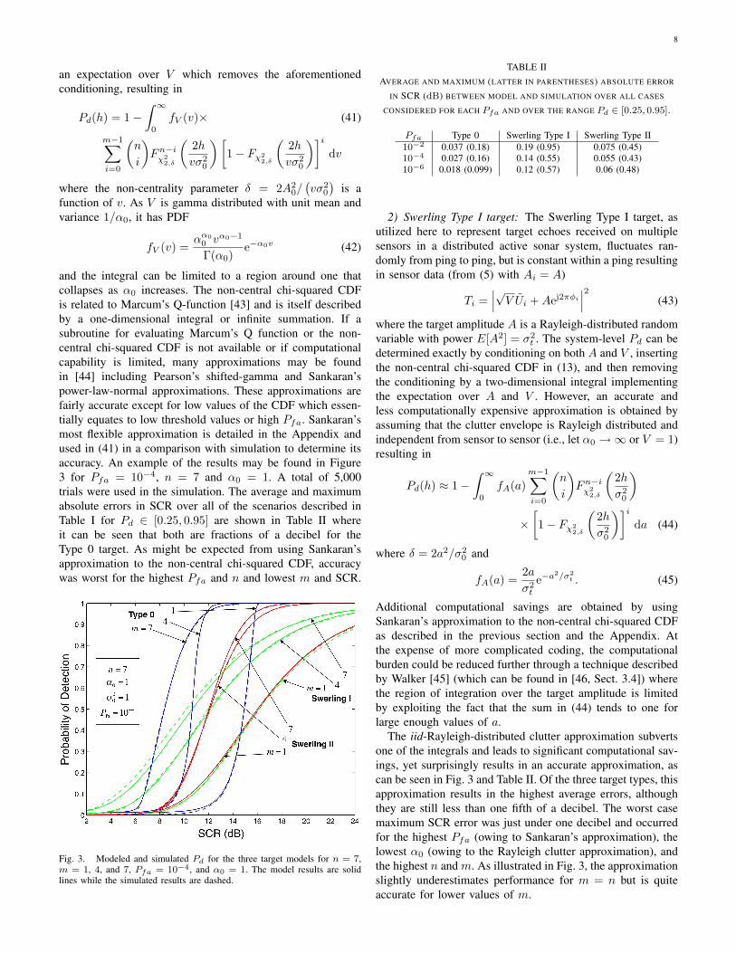
The use of multiple sensors in distributed detection isintended to increase system-level performance by increasingcoverage and/or system-level Pd for a fixed Pfa. This improve-ment in the Pd-Pfa fusion receiver operating characteristic(ROC) curves is illustrated in Figs. 4–6 for the three targetmodels. In each figure, the OR processor (m = 1), ANDprocessor (m = n), and median processor (m = (n + 1)/2)

are evaluated for increasing numbers of sensors (n = 1, 3, 7,11, and 21), heavy clutter (α0 = 1), and moderate levels ofSCR. In Fig. 4 it is seen that the AND processor provides thebest performance for the Type 0 target at low values of Pfawhile the OR processor provides little or no performance gain(Pd is only increasing with n when the sensor-level Pd is veryhigh). The median processor provides the best performance atmoderate values of Pfa (e.g., above about 5 × 10−5 ). Asillustrated here and in the following section, the best value ofm depends on many factors.

The fusion ROC curves shown in Fig. 5 for the SwerlingType I target are similar to those for the Type 0 target althoughthe median processor is only better than the AND processorfor Pfa above about 10−2. The improvement in system-levelPd for a fixed Pfa for the AND and median processors is alsonot as significant for the Swerling Type I target compared withthat observed for the Type 0 target in Fig. 4.

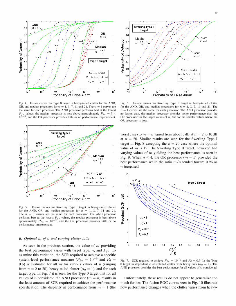
In Fig. 6 the fusion ROC curves for the Swerling TypeII target show that the median processor provides the bestperformance for larger values of n (11 and 21) while the ORprocessor is best for smaller values of n. The AND processorprovided no fusion gain regardless of the number of sensors—note that all the AND fusion ROC curves overlay eachother—yielding an identical result to the case of a fluctuatingtarget in independent Rayleigh-distributed clutter. This may beexplained by relating the sensor-level threshold for fusing nsensors (hn) to that for fusing one (h1) and then showing that,for a fixed the system-level Pfa, the system-level Pd does notchange with n. Conditioning on V , the sensor data are iidexponentially distributed with mean λ = V σ2

0 + σ2t and the

system-level detection statistic for the AND processor is T(1),the minimum order statistic. The minimum of n iid exponentialrandom variables with mean λ is also exponentially distributedbut with mean λ/n. Thus, the system level threshold may beobtained by inverting

Pfa = EV

[Pr{UV σ2

0

n> hn |V

}](47)

for hn where U is exponentially distributed with unit mean.From (47) it is clear that the threshold for combining n sensorsis related to that for just one sensor according to hn = h1/n.Substituting this into the system-level Pd,

Pd(n) = EV

[Pr

{U(V σ2

0 + σ2t

)n

> hn |V

}]= EV

[Pr{U(V σ2

0 + σ2t

)> h1 |V

}]= Pd(1), (48)

illustrates the invariance of detection performance with n. Thedistribution of V in (47) and (48) will change the specificvalues of hn and Pd(n), but does not alter the relationshipshn = h1/n and Pd(n) = Pd(1) indicating that no fusion gainmay be obtained for a Swerling Type II target using the ANDprocessor irrespective of whether the clutter data are Rayleigh,K, or some other distribution as long as the data follow thecorrelated clutter model described by (5).

10

Fig. 4. Fusion curves for Type 0 target in heavy-tailed clutter for the AND,OR, and median processors for n = 1, 3, 7, 11 and 21. The n = 1 curves arethe same for each processor. The AND processor performs best at the lowestPfa values, the median processor is best above approximately Pfa = 5 ×10−5, and the OR processor provides little or no performance improvement.

Fig. 5. Fusion curves for Swerling Type I target in heavy-tailed clutterfor the AND, OR, and median processors for n = 1, 3, 7, 11 and 21.The n = 1 curves are the same for each processor. The AND processorperforms best at the lowest Pfa values, the median processor is best aboveapproximately Pfa = 10−2, and the OR processor provides little or noperformance improvement.

B. Optimal m of n and varying clutter tails

As seen in the previous section, the value of m providingthe best performance varies with target type, n, and Pfa. Toexamine this variation, the SCR required to achieve a specificsystem-level performance measure (Pfa = 10−6 and Pd =0.5) is evaluated for all m for various values of n (rangingfrom n = 2 to 20), heavy-tailed clutter (α0 = 1), and for eachtarget type. In Fig. 7 it is seen for the Type 0 target that for allvalues of n considered the AND processor (m = n) results inthe least amount of SCR required to achieve the performancespecification. The disparity in performance from m = 1 (the

Fig. 6. Fusion curves for Swerling Type II target in heavy-tailed clutterfor the AND, OR, and median processors for n = 1, 3, 7, 11 and 21. Then = 1 curves are the same for each processor. The AND processor providesno fusion gain, the median processor provides better performance than theOR processor for the larger values of n, but not the smaller values where theOR processor is best.

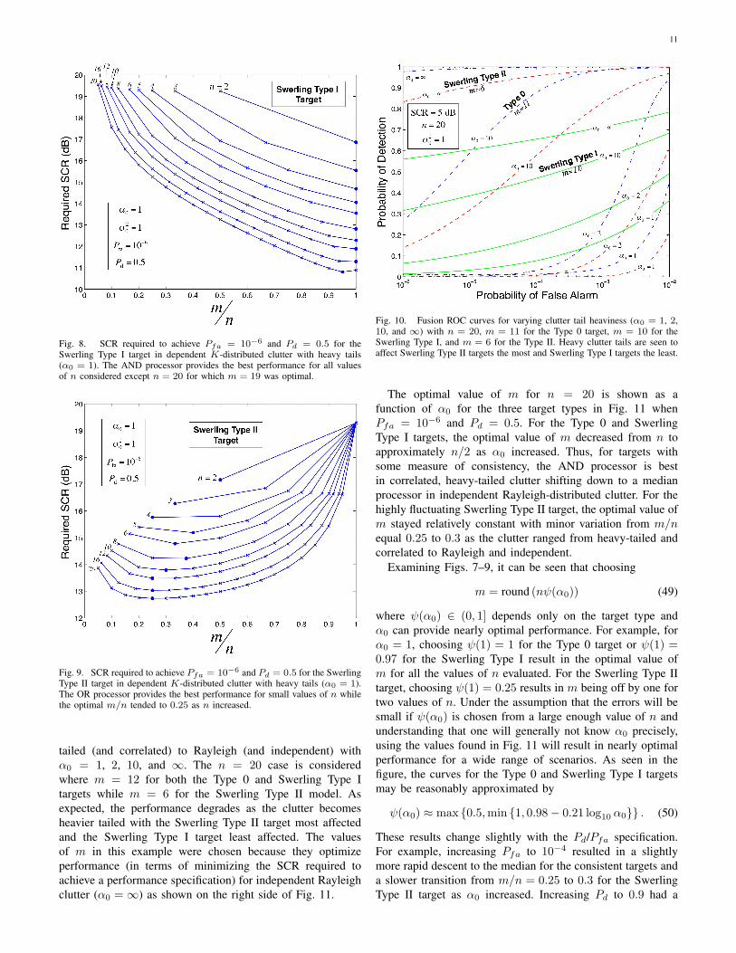
worst case) to m = n varied from about 3 dB at n = 2 to 10 dBat n = 20. Similar results are seen for the Swerling Type Itarget in Fig. 8 excepting the n = 20 case where the optimalvalue of m is 19. The Swerling Type II target, however, hadvarying values of m yielding the best performance as seen inFig. 9. When n ≤ 4, the OR processor (m = 1) provided thebest performance while the ratio m/n tended toward 0.25 asn increased.

Fig. 7. SCR required to achieve Pfa = 10−6 and Pd = 0.5 for the Type0 target in dependent K-distributed clutter with heavy tails (α0 = 1). TheAND processor provides the best performance for all values of n considered.

Unfortunately, these results do not appear to generalize toomuch further. The fusion ROC curves seen in Fig. 10 illustratehow performance changes when the clutter varies from heavy-

11

Fig. 8. SCR required to achieve Pfa = 10−6 and Pd = 0.5 for theSwerling Type I target in dependent K-distributed clutter with heavy tails(α0 = 1). The AND processor provides the best performance for all valuesof n considered except n = 20 for which m = 19 was optimal.

Fig. 9. SCR required to achieve Pfa = 10−6 and Pd = 0.5 for the SwerlingType II target in dependent K-distributed clutter with heavy tails (α0 = 1).The OR processor provides the best performance for small values of n whilethe optimal m/n tended to 0.25 as n increased.

tailed (and correlated) to Rayleigh (and independent) withα0 = 1, 2, 10, and ∞. The n = 20 case is consideredwhere m = 12 for both the Type 0 and Swerling Type Itargets while m = 6 for the Swerling Type II model. Asexpected, the performance degrades as the clutter becomesheavier tailed with the Swerling Type II target most affectedand the Swerling Type I target least affected. The valuesof m in this example were chosen because they optimizeperformance (in terms of minimizing the SCR required toachieve a performance specification) for independent Rayleighclutter (α0 =∞) as shown on the right side of Fig. 11.

Fig. 10. Fusion ROC curves for varying clutter tail heaviness (α0 = 1, 2,10, and ∞) with n = 20, m = 11 for the Type 0 target, m = 10 for theSwerling Type I, and m = 6 for the Type II. Heavy clutter tails are seen toaffect Swerling Type II targets the most and Swerling Type I targets the least.

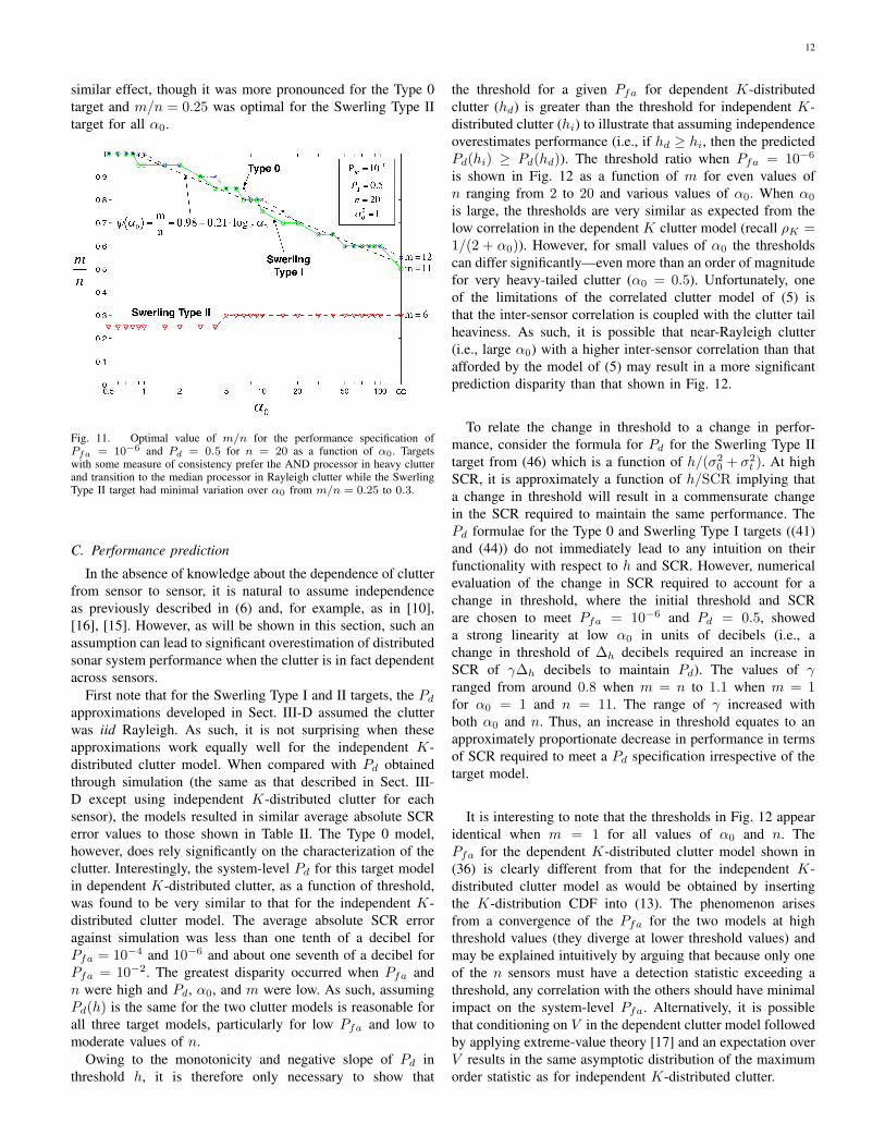
The optimal value of m for n = 20 is shown as afunction of α0 for the three target types in Fig. 11 whenPfa = 10−6 and Pd = 0.5. For the Type 0 and SwerlingType I targets, the optimal value of m decreased from n toapproximately n/2 as α0 increased. Thus, for targets withsome measure of consistency, the AND processor is bestin correlated, heavy-tailed clutter shifting down to a medianprocessor in independent Rayleigh-distributed clutter. For thehighly fluctuating Swerling Type II target, the optimal value ofm stayed relatively constant with minor variation from m/nequal 0.25 to 0.3 as the clutter ranged from heavy-tailed andcorrelated to Rayleigh and independent.

Examining Figs. 7–9, it can be seen that choosing

m = round (nψ(α0)) (49)

where ψ(α0) ∈ (0, 1] depends only on the target type andα0 can provide nearly optimal performance. For example, forα0 = 1, choosing ψ(1) = 1 for the Type 0 target or ψ(1) =0.97 for the Swerling Type I result in the optimal value ofm for all the values of n evaluated. For the Swerling Type IItarget, choosing ψ(1) = 0.25 results in m being off by one fortwo values of n. Under the assumption that the errors will besmall if ψ(α0) is chosen from a large enough value of n andunderstanding that one will generally not know α0 precisely,using the values found in Fig. 11 will result in nearly optimalperformance for a wide range of scenarios. As seen in thefigure, the curves for the Type 0 and Swerling Type I targetsmay be reasonably approximated by

ψ(α0) ≈ max {0.5,min {1, 0.98− 0.21 log10 α0}} . (50)

These results change slightly with the Pd/Pfa specification.For example, increasing Pfa to 10−4 resulted in a slightlymore rapid descent to the median for the consistent targets anda slower transition from m/n = 0.25 to 0.3 for the SwerlingType II target as α0 increased. Increasing Pd to 0.9 had a

12

similar effect, though it was more pronounced for the Type 0target and m/n = 0.25 was optimal for the Swerling Type IItarget for all α0.

Fig. 11. Optimal value of m/n for the performance specification ofPfa = 10−6 and Pd = 0.5 for n = 20 as a function of α0. Targetswith some measure of consistency prefer the AND processor in heavy clutterand transition to the median processor in Rayleigh clutter while the SwerlingType II target had minimal variation over α0 from m/n = 0.25 to 0.3.

C. Performance prediction

In the absence of knowledge about the dependence of clutterfrom sensor to sensor, it is natural to assume independenceas previously described in (6) and, for example, as in [10],[16], [15]. However, as will be shown in this section, such anassumption can lead to significant overestimation of distributedsonar system performance when the clutter is in fact dependentacross sensors.

First note that for the Swerling Type I and II targets, the Pdapproximations developed in Sect. III-D assumed the clutterwas iid Rayleigh. As such, it is not surprising when theseapproximations work equally well for the independent K-distributed clutter model. When compared with Pd obtainedthrough simulation (the same as that described in Sect. III-D except using independent K-distributed clutter for eachsensor), the models resulted in similar average absolute SCRerror values to those shown in Table II. The Type 0 model,however, does rely significantly on the characterization of theclutter. Interestingly, the system-level Pd for this target modelin dependent K-distributed clutter, as a function of threshold,was found to be very similar to that for the independent K-distributed clutter model. The average absolute SCR erroragainst simulation was less than one tenth of a decibel forPfa = 10−4 and 10−6 and about one seventh of a decibel forPfa = 10−2. The greatest disparity occurred when Pfa andn were high and Pd, α0, and m were low. As such, assumingPd(h) is the same for the two clutter models is reasonable forall three target models, particularly for low Pfa and low tomoderate values of n.

Owing to the monotonicity and negative slope of Pd inthreshold h, it is therefore only necessary to show that

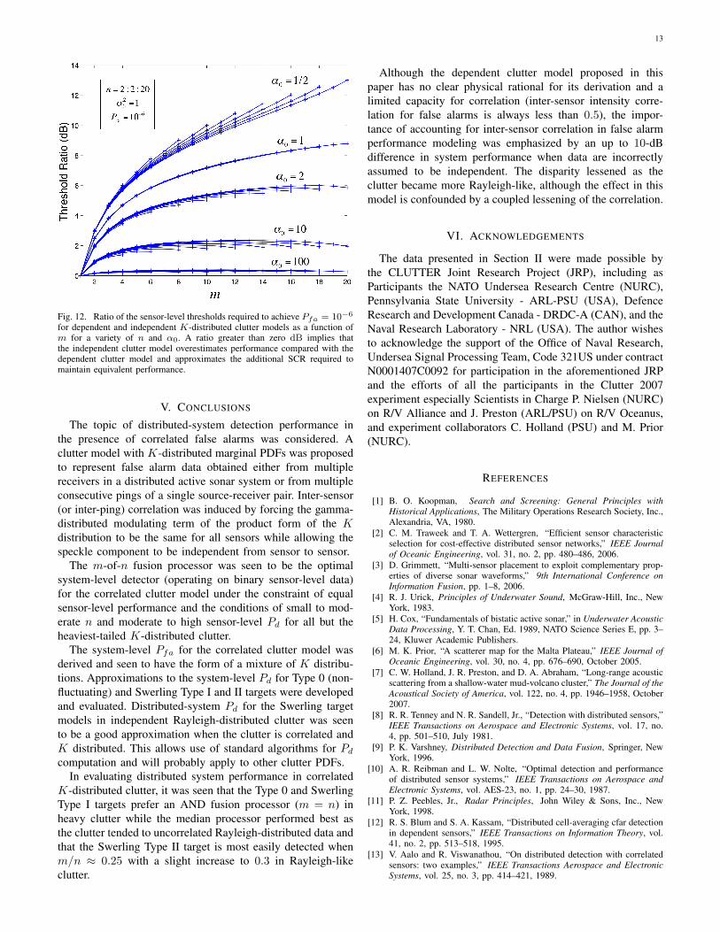
the threshold for a given Pfa for dependent K-distributedclutter (hd) is greater than the threshold for independent K-distributed clutter (hi) to illustrate that assuming independenceoverestimates performance (i.e., if hd ≥ hi, then the predictedPd(hi) ≥ Pd(hd)). The threshold ratio when Pfa = 10−6

is shown in Fig. 12 as a function of m for even values ofn ranging from 2 to 20 and various values of α0. When α0

is large, the thresholds are very similar as expected from thelow correlation in the dependent K clutter model (recall ρK =1/(2 + α0)). However, for small values of α0 the thresholdscan differ significantly—even more than an order of magnitudefor very heavy-tailed clutter (α0 = 0.5). Unfortunately, oneof the limitations of the correlated clutter model of (5) isthat the inter-sensor correlation is coupled with the clutter tailheaviness. As such, it is possible that near-Rayleigh clutter(i.e., large α0) with a higher inter-sensor correlation than thatafforded by the model of (5) may result in a more significantprediction disparity than that shown in Fig. 12.

To relate the change in threshold to a change in perfor-mance, consider the formula for Pd for the Swerling Type IItarget from (46) which is a function of h/(σ2

0 + σ2t ). At high

SCR, it is approximately a function of h/SCR implying thata change in threshold will result in a commensurate changein the SCR required to maintain the same performance. ThePd formulae for the Type 0 and Swerling Type I targets ((41)and (44)) do not immediately lead to any intuition on theirfunctionality with respect to h and SCR. However, numericalevaluation of the change in SCR required to account for achange in threshold, where the initial threshold and SCRare chosen to meet Pfa = 10−6 and Pd = 0.5, showeda strong linearity at low α0 in units of decibels (i.e., achange in threshold of ∆h decibels required an increase inSCR of γ∆h decibels to maintain Pd). The values of γranged from around 0.8 when m = n to 1.1 when m = 1for α0 = 1 and n = 11. The range of γ increased withboth α0 and n. Thus, an increase in threshold equates to anapproximately proportionate decrease in performance in termsof SCR required to meet a Pd specification irrespective of thetarget model.

It is interesting to note that the thresholds in Fig. 12 appearidentical when m = 1 for all values of α0 and n. ThePfa for the dependent K-distributed clutter model shown in(36) is clearly different from that for the independent K-distributed clutter model as would be obtained by insertingthe K-distribution CDF into (13). The phenomenon arisesfrom a convergence of the Pfa for the two models at highthreshold values (they diverge at lower threshold values) andmay be explained intuitively by arguing that because only oneof the n sensors must have a detection statistic exceeding athreshold, any correlation with the others should have minimalimpact on the system-level Pfa. Alternatively, it is possiblethat conditioning on V in the dependent clutter model followedby applying extreme-value theory [17] and an expectation overV results in the same asymptotic distribution of the maximumorder statistic as for independent K-distributed clutter.

13

Fig. 12. Ratio of the sensor-level thresholds required to achieve Pfa = 10−6

for dependent and independent K-distributed clutter models as a function ofm for a variety of n and α0. A ratio greater than zero dB implies thatthe independent clutter model overestimates performance compared with thedependent clutter model and approximates the additional SCR required tomaintain equivalent performance.

V. CONCLUSIONS

The topic of distributed-system detection performance inthe presence of correlated false alarms was considered. Aclutter model with K-distributed marginal PDFs was proposedto represent false alarm data obtained either from multiplereceivers in a distributed active sonar system or from multipleconsecutive pings of a single source-receiver pair. Inter-sensor(or inter-ping) correlation was induced by forcing the gamma-distributed modulating term of the product form of the Kdistribution to be the same for all sensors while allowing thespeckle component to be independent from sensor to sensor.

The m-of-n fusion processor was seen to be the optimalsystem-level detector (operating on binary sensor-level data)for the correlated clutter model under the constraint of equalsensor-level performance and the conditions of small to mod-erate n and moderate to high sensor-level Pd for all but theheaviest-tailed K-distributed clutter.

The system-level Pfa for the correlated clutter model wasderived and seen to have the form of a mixture of K distribu-tions. Approximations to the system-level Pd for Type 0 (non-fluctuating) and Swerling Type I and II targets were developedand evaluated. Distributed-system Pd for the Swerling targetmodels in independent Rayleigh-distributed clutter was seento be a good approximation when the clutter is correlated andK distributed. This allows use of standard algorithms for Pdcomputation and will probably apply to other clutter PDFs.

In evaluating distributed system performance in correlatedK-distributed clutter, it was seen that the Type 0 and SwerlingType I targets prefer an AND fusion processor (m = n) inheavy clutter while the median processor performed best asthe clutter tended to uncorrelated Rayleigh-distributed data andthat the Swerling Type II target is most easily detected whenm/n ≈ 0.25 with a slight increase to 0.3 in Rayleigh-likeclutter.

Although the dependent clutter model proposed in thispaper has no clear physical rational for its derivation and alimited capacity for correlation (inter-sensor intensity corre-lation for false alarms is always less than 0.5), the impor-tance of accounting for inter-sensor correlation in false alarmperformance modeling was emphasized by an up to 10-dBdifference in system performance when data are incorrectlyassumed to be independent. The disparity lessened as theclutter became more Rayleigh-like, although the effect in thismodel is confounded by a coupled lessening of the correlation.

VI. ACKNOWLEDGEMENTS

The data presented in Section II were made possible bythe CLUTTER Joint Research Project (JRP), including asParticipants the NATO Undersea Research Centre (NURC),Pennsylvania State University - ARL-PSU (USA), DefenceResearch and Development Canada - DRDC-A (CAN), and theNaval Research Laboratory - NRL (USA). The author wishesto acknowledge the support of the Office of Naval Research,Undersea Signal Processing Team, Code 321US under contractN0001407C0092 for participation in the aforementioned JRPand the efforts of all the participants in the Clutter 2007experiment especially Scientists in Charge P. Nielsen (NURC)on R/V Alliance and J. Preston (ARL/PSU) on R/V Oceanus,and experiment collaborators C. Holland (PSU) and M. Prior(NURC).

REFERENCES

[1] B. O. Koopman, Search and Screening: General Principles withHistorical Applications, The Military Operations Research Society, Inc.,Alexandria, VA, 1980.

[2] C. M. Traweek and T. A. Wettergren, “Efficient sensor characteristicselection for cost-effective distributed sensor networks,” IEEE Journalof Oceanic Engineering, vol. 31, no. 2, pp. 480–486, 2006.

[3] D. Grimmett, “Multi-sensor placement to exploit complementary prop-erties of diverse sonar waveforms,” 9th International Conference onInformation Fusion, pp. 1–8, 2006.

[4] R. J. Urick, Principles of Underwater Sound, McGraw-Hill, Inc., NewYork, 1983.

[5] H. Cox, “Fundamentals of bistatic active sonar,” in Underwater AcousticData Processing, Y. T. Chan, Ed. 1989, NATO Science Series E, pp. 3–24, Kluwer Academic Publishers.

[6] M. K. Prior, “A scatterer map for the Malta Plateau,” IEEE Journal ofOceanic Engineering, vol. 30, no. 4, pp. 676–690, October 2005.

[7] C. W. Holland, J. R. Preston, and D. A. Abraham, “Long-range acousticscattering from a shallow-water mud-volcano cluster,” The Journal of theAcoustical Society of America, vol. 122, no. 4, pp. 1946–1958, October2007.

[8] R. R. Tenney and N. R. Sandell, Jr., “Detection with distributed sensors,”IEEE Transactions on Aerospace and Electronic Systems, vol. 17, no.4, pp. 501–510, July 1981.

[9] P. K. Varshney, Distributed Detection and Data Fusion, Springer, NewYork, 1996.

[10] A. R. Reibman and L. W. Nolte, “Optimal detection and performanceof distributed sensor systems,” IEEE Transactions on Aerospace andElectronic Systems, vol. AES-23, no. 1, pp. 24–30, 1987.

[11] P. Z. Peebles, Jr., Radar Principles, John Wiley & Sons, Inc., NewYork, 1998.

[12] R. S. Blum and S. A. Kassam, “Distributed cell-averaging cfar detectionin dependent sensors,” IEEE Transactions on Information Theory, vol.41, no. 2, pp. 513–518, 1995.

[13] V. Aalo and R. Viswanathou, “On distributed detection with correlatedsensors: two examples,” IEEE Transactions Aerospace and ElectronicSystems, vol. 25, no. 3, pp. 414–421, 1989.

14

[14] P. Willett, P. F. Swaszek, and R. S. Blum, “The good, bad and ugly:distributed detection of a known signal in dependent gaussian noise,”IEEE Transactions on Signal Processing, vol. 48, no. 12, pp. 3266–3279, 2000.

[15] C. H. Gowda and R. Viswanathan, “Performance of distributed cfar testunder various clutter amplitudes,” IEEE Transactions Aerospace andElectronic Systems, vol. 35, no. 4, pp. 1410–1419, 1999.

[16] R. Viswanathan and A. Ansari, “Distributed detection of a signal ingeneralized gaussian noise,” IEEE Transactions on Acoustics, Speechand Signal Processing, vol. 37, no. 5, pp. 775–778, 1989.

[17] H. A. David, Order Statistics, John Wiley & Sons, Inc., New York,1981.

[18] E. Jakeman and P. N. Pusey, “A model for non-Rayleigh sea echo,”IEEE Transactions on Antennas and Propagation, vol. 24, no. 6, pp.806–814, November 1976.

[19] M. Sandys-Wunsch and M. G. Hazen, “Multistatic localization error dueto receiver positioning errors,” IEEE Journal of Oceanic Engineering,vol. 27, no. 2, pp. 328–334, 2002.

[20] S. Coraluppi and C. Carthel, “Distributed tracking in multistage sonar,”Aerospace and Electronic Systems, IEEE Transactions on, vol. 41, no.3, pp. 1138–1147, 2005.

[21] C. G. Hempel, “Adaptive track detection for multi-static active sonarsystems,” OCEANS 2006, pp. 1–6, 2006.

[22] B. K. Newhall, “Continuous reverberation response and comb spectrawaveform design,” IEEE Journal of Oceanic Engineering, vol. 32, no.2, pp. 524–532, 2007.

[23] O. E. Drummond, “Track and tracklet fusion filtering,” in Proc. SPIE,Signal and Data Processing of Small Targets, 2002, vol. 4728, pp. 176–195.

[24] E. Chang, D. S. Marx, M. A. Nelson, W. D. Gillespie, A. Putney, L. K.Warman, R. E. Chatham, and B.N Barrett, “Long range active syntheticaperture sonar results,” in OCEANS 2000 MTS/IEEE Conference, 2000,vol. 1, pp. 1–5.

[25] H. C. Song, W. S. Hodgkiss, W. A. Kuperman, P. Roux, and T. Akal,“Experimental demonstration of adaptive reverberation nulling usingtime reversal,” The Journal of the Acoustical Society of America, vol.118, no. 3, pp. 1381–1387, September 2005.

[26] D. A. Abraham and P. K. Willett, “Active sonar detection in shallowwater using the Page test,” IEEE Journal of Oceanic Engineering, vol.27, no. 1, pp. 35–46, 2002.

[27] D. A. Abraham and A. P. Lyons, “Novel physical interpretations of K-distributed reverberation,” IEEE Journal of Oceanic Engineering, vol.27, no. 4, pp. 800–813, October 2002.

[28] J. R. Preston and D. A. Abraham, “Non-Rayleigh reverberation charac-teristics near 400 Hz observed on the New Jersey Shelf,” IEEE Journalof Oceanic Engineering, vol. 29, no. 2, pp. 215–235, April 2004.

[29] E. Jakeman, “Scattering by a corrugated random surface with fractalslope,” Journal of Physics A: Mathematical and General, vol. 15, no.2, pp. L55–L59, 1982.

[30] K. D. Ward, “Compound representation of high resolution sea clutter,”Electronics Letters, vol. 17, no. 16, pp. 561–563, August 1981.

[31] D. A. Abraham, “Signal excess in K-distributed reverberation,” IEEEJournal of Oceanic Engineering, vol. 28, no. 3, pp. 526–536, July 2003.

[32] B. C. Armstrong and H. D. Griffiths, “CFAR detection of fluctuatingtargets in spatially correlated K-distributed clutter,” IEE Proceedings-F,Radar and Signal Processing, vol. 138, no. 2, pp. 139–152, April 1991.

[33] S. Watts, “Cell-averaging cfar gain in spatially correlated k-distributedclutter,” IEE Proceedings - Radar, Sonar and Navigation, vol. 143, no.5, pp. 321–327, 1996.

[34] M. Barkat and F. Soltani, “Cell-averaging cfar detection in compoundclutter with spatially correlated texture and speckle,” IEE Proceedings- Radar, Sonar and Navigation, vol. 146, no. 6, pp. 279–284, 1999.

[35] J. S. Lee, D. L. Schuler, R. H. Lang, and K. J. Ranson, “K-distributionfor multi-look processed polarimetric sar imagery,” in Proceedings ofGeoscience and Remote Sensing Symposium, 1994, vol. 4, pp. 2179–2181.

[36] E. Conte and M. Longo, “Characterisation of radar clutter as aspherically invariant random process,” IEE Proceedings-F, Radar andSignal Processing, vol. 134, no. 2, pp. 191–197, April 1987.

[37] T. J. Barnard and F. Khan, “Statistical normalization of sphericallyinvariant non-Gaussian clutter,” IEEE Journal of Oceanic Engineering,vol. 29, no. 2, pp. 303–309, April 2004.

[38] R. V. Hogg and A. T. Craig, Introduction to Mathematical Statistics,Macmillan Pub. Co., New York, fourth edition, 1978.

[39] E. L. Lehmann, Testing Statistical Hypotheses, John Wiley & Sons,Inc., New York, second edition, 1986.

[40] J. F. Hurley, Intermediate Calculus: Multivariable Functions and Dif-ferential Equations with Applications, Saunders College, Philidelphia,PA, 1980.

[41] I. S. Gradshteyn and I. M. Ryzhik, Table of Integrals, Series, andProducts, Elsevier Academic Press, Burlington, MA, seventh edition,2007, Edited by A. Jeffrey and D. Zwillinger.

[42] W. Feller, An Introduction to Probability Theory and Its Applications,vol. II, John Wiley & Sons, second edition, 1971.

[43] H. L. Van Trees, Detection, Estimation, and Modulation Theory: PartI, John Wiley & Sons, Inc., New York, 1968.

[44] N. L. Johnson, S. Kotz, and N. Balakrishnan, Continuous UnivariateDistributions, vol. 2, John Wiley & Sons, Inc., New York, secondedition, 1995.

[45] J. F. Walker, “Performance data for a double-threshold detection radar,”IEEE Transactions Aerospace and Electronic Systems, vol. AES-7, no.1, pp. 142–146, January 1971.

[46] D. Schleher, Ed., Automatic Detection and Radar Data Processing,Artech House, Inc., Norwood, Massachusetts, 1980.

APPENDIX

As described in [44, eq. 29.61d], Sankaran approximated anon-central chi-squared random variable with a normal variateraised to a power. The resulting CDF approximation is

Fχ2ν,δ

(x) ≈ Φ

(σ−1z

[(x

ν + δ

)hz− µz

])(51)

where ν is the degrees-of-freedom parameter, δ the non-centrality parameter, Φ(z) is the standard-normal CDF,

hz = 1− 23

(ν + δ)(ν + 3δ)(ν + 2δ)−2, (52)

µz = 1 + hz(hz − 1)(ν + 2δ)(ν + δ)2

−hz(hz − 1)(hz − 2)(3hz − 1)(ν + 2δ)2(ν + δ)4

, (53)

and

σ2z = 2h2

z

(ν + 2δ)(ν + δ)2

[1− (hz − 1)(3hz − 1)

(ν + 2δ)(ν + δ)2

]. (54)