Distributed Constrained Optimization for Bayesian OpportunisticVisual Sensing

Akshay A. Morye, Chong Ding, Amit K. Roy-Chowdhury, Jay A. Farrell

Abstract—We propose a control mechanism to obtain oppor-tunistic high resolution facial imagery, via distributed constrainedoptimization of the PTZ parameters for each camera in a sensornetwork. The objective function of the optimization problemquantifies the per camera per target image quality. The trackingconstraints, which are a lower bound on the information aboutthe estimated position for each target, define the feasible PTZparameter space. Each camera alters its own PTZ settings. Allcameras use information broadcast by neighboring cameras suchthat the PTZ parameters of all cameras are simultaneouslyoptimized relative to the global objective. At certain times ofopportunity, due to the configuration of the targets relative to thecameras, and the fact that each camera may track many targets,the camera network may be able to reconfigure itself to achievethe tracking specification for all targets with remaining degrees-of-freedom that can be used to obtain high-res facial imagesfrom desirable aspect angles for certain targets. The challengeis to define algorithms to automatically find these time instants,the appropriate imaging camera, and the appropriate parametersettings for all cameras to capitalize on these opportunities. Thesolution proposed herein involves a Bayesian formulation in agame theoretic setting. The Bayesian formulation automaticallytrades off objective maximization versus the risk of losingtrack of any target. The article describes the problem andsolution formulations, design of aligned local and global objectivefunctions and the inequality constraint set, and developmentof a Distributed Lagrangian Consensus algorithm that allowscameras to exchange information and asymptotically convergeon a pair of primal-dual optimal solutions. This article presentsthe theoretical solution along with simulation results.

Index Terms—Camera Sensor Networks, Cooperative Control,Distributed Constrained Optimization.

I. INTRODUCTION

Static camera networks have a lower per camera cost ofinstallation than pan, tilt, zoom (PTZ) camera sensor networks;however, PTZ camera networks can have lower total installa-tion cost with greater performance. Static camera networksmust be designed to achieve the coverage and tracking speci-fications given worst case target distributions. Installation costconstraints can lead to imagery sequences from static cameranetwork applications that are quite challenging to analyze. PTZcamera networks, with appropriate software and communica-tions, can dynamically reconfigure in response to applicationevents and actual target distributions to optimize the acquiredimagery sequences accounting for viewpoints and resolution,to facilitate image analysis and scene understanding.

A prototypical application is a security screening checkpointat the entrance lobby of a building. Over the course of eachday a high volume of people flow through the room. Theroom is equipped with a fixed number of cameras while the

A. A. Morye, A. K. Roy-Chowdhury and J. A. Farrell are with the Dept.of EE, U. of CA Riverside, CA, 92521 USA. e-mail: amorye@ee.ucr.edu

C. Ding is with the Dept. of CSE, U. of CA Riverside, CA, 92521 USA

number and location of people in the room varies with time.The objective of the camera network is to track (i.e., stateestimation) all persons in the room at a specified accuracy levelat all times and to capture high-res facial images for certainpersons in the room at opportunistically selected instants.

The challenges of such an application are development ofalgorithms to ensure accurate propagation of target-relatedinformation throughout the distributed network, analysis of theeffect of changing network topology on solution convergence,design of distributed PTZ optimization algorithms, and thedesign of objective functions suitable to solving the specifiedproblem that also have the properties necessary to ensureconvergence. All these factors influence the selection of anoptimization strategy. In this paper, we formulate the problemwithin a Bayesian game theoretic framework and utilize adistributed constrained optimization approach to compute theoptimal PTZ settings that achieve the global camera networkobjective through optimization of local camera objectives.

II. LITERATURE REVIEW

The research proposed herein falls within the scope of activecomputer vision [1], which involves research on cooperationand coordination between many cameras in a network, forapplications such as autonomous surveillance, simultaneouslocalization and mapping (SLAM), trajectory planning, etc.

Assuming predesigned static camera placement given cer-tain tasks, the articles [2], [3] define deployment strategiesfor camera networks. A path-planning based approach isproposed in [4], where static cameras track targets, and PTZcameras obtain high-res images. Given a target activity map,the Expectation-Maximization algorithm [5] is used to performarea coverage in [6]. Other interesting active vision problemssuch as object detection across cameras, camera handoff, andcamera configuration, with an emphasis on camera networksis addressed in [7]–[10]. Methods for tracking a group ofpeople in a multi-camera setup are addressed in [11], [12].A review of human motion analysis is performed in [13]. Themethods proposed therein dealt with a centralized processingscheme and did not delve into the decentralized organization ofcameras. Distributed computer vision algorithms are studied in[14], [15]. Distributed state estimation algorithms over visionnetworks are studied in [16]–[18]. The above articles do notfocus on distributed optimization of the PTZ parameters tooptimize the acquired imagery.

Assumptions on the camera network communication topol-ogy play a major role in the problem solution. Preliminarywork on camera networks using independent cameras that lackcoordination is provided in [19]. A machine learning-basedmethod to learn the network topology is described in [20].

The authors employ unsupervised machine learning to estab-lish links between target activity and the associated cameraviews to decipher communication topology to determine targettracks. In [21], authors measure the statistical dependencebetween observations in multiple camera views to quantifya potential interconnecting pathway for target tracks betweendifferent camera views with an aim to enable camera handoff.Multi-agent systems with switching topologies are studied in[22], [23]. Though the studies therein are not based on visualsensing applications, [22], [23] provide significant insight onmethods potentially applicable to mobile camera networks.

A recent research survey [14] identifies various computer vi-sion problems that can be solved in a distributed fashion withina network topology. Within a distributed framework, problemsare often defined as multi-agent tasks that utilize cooperationbetween agents. A vision-based target pose estimation problemthat employs cooperation and uses multi-agent optimizationtechniques is addressed in [24]. Therein, authors propose apassivity-based target motion observer model, and proposea cooperative estimation algorithm where every agent solvesan unconstrained convex minimization problem to minimizeestimation error. The passivity based motion observer model isutilized in [25] for camera control, under assumptions on targetmotion. Though the articles above focus on target and camerapose estimation, the challenges related to obtaining high-resimagery while maintaining state estimation performance arenot considered.

A survey of automated visual surveillance systems is pro-vided in [26]. Building scene interpretation in a modularmanner on decentralized intelligent multi-camera surveillancesystems is described in [27]. For multi-agent network systemsthat employ a time-varying topology, stability analysis isprovided in [28]. The analysis is based on graph-theoretic toolswhere the authors assume the problem to be convex.

Game-theory as a tool for designing solutions to multi-agentproblems is described in [29]. A vehicle-target assignmentproblem within the game-theoretic framework was proposedin [30]. The standard target assignment problem is differentfrom a camera-target assignment problem in that the prob-lem described therein is a one-to-one mapping problem withthe stationary targets, whereas the camera-target assignmentproblem allows multiple cameras to each track multiple mov-ing targets. Nonetheless, articles [29], [30] provide valuableinsight into the challenges faced while designing the cameraparameter optimization as a cooperative game played bymultiple cameras.

A game-theoretic camera control approach for collabora-tive sensing is proposed in [31]–[34]. In [31], the agentscollaborate to optimize a cost function that is the weightedcombination of area coverage over regions of interest whiletrying to achieve high-res images of specific (highly weighted)targets. In [32]–[34], the agents account for risk and includeimage quality in a weighted cost function. Collaboration wasensured through a game-theoretic formulation. The quality ofthe solution was dependent on the user-defined weights.

An automated annealing approach for updating Lagrangemultipliers within a constrained optimization framework toreduce dependence on agent inter-communication is provided

in [35]. The method uses the probability collectives frameworkto generate a relation between game theory and statisticalphysics. The authors use a game-theoretic motivation to de-velop a parallel algorithm, but consider a non-cooperativegame between agents, where the action of one agent iscompletely independent of the other agents in the network.Such an assumption is not appropriate for our application.

A systematic methodology for designing agent objectivefunctions is outlined in [36], using a hierarchical decoupling ofthe global objective function into local objective functions thatare aligned with the global function. Each agent is modeledas a self-interested decision maker within a game-theoreticenvironment, then convergence proofs from the game theoryliterature are utilized. Herein, we utilize the methodology of[36] to decompose a Bayesian value function designed forthe opportunistic visual sensing application into local valuefunctions suitable for distributed implementation.

III. CONTRIBUTIONS OF THE PAPER

The distributed PTZ camera parameter optimization prob-lem considered herein is similar to the class of problemsconsidered in [32], [33]. The solution methodology herein issignificantly enhanced. The cost function in [33] is a weightedsummation of competing objectives and the optimization isunconstrained. In [32], the authors use a heuristic to weight thehigh-res imaging objective dependent on the quality of targettracking performance achieved by the network of cameras,collectively. Although such an approach allows the networkof cameras to obtain high-res images only if the trackingheuristic is desirable, there is no guarantee of all targets beingtracked to the required tracking specification. Optimizationis accomplished via sequential utility maximization by eachagent. Neither paper includes an analysis of convergence of thedistributed implementation. These issues are further discussedin Remark 3 after defining the required notation.

Herein, a method for distributed, cooperative and paralleloptimization on a connected camera network is defined, ana-lyzed, and implemented. The camera parameter optimizationprocess maximizes a Bayesian value function that accounts forrisk arising from the uncertainty in the estimated target posi-tions, while adhering to Bayesian constraints on the trackingperformance. The value function is designed as an ordinalpotential function [36], such that it can be decoupled intolocal objectives known to each camera. The tracking constraintis common to all cameras. With reasonable assumptions onnetwork connectivity, utilizing a Bayesian constrained opti-mization approach, the proposed solution method providesfeasible optimal solutions to perform opportunistic visualsensing of targets maneuvering with random trajectories.

A shorter and less comprehensive presentation of thisapproach is contained in [34]. Relative to [34], this articleincludes an enhanced discussion and analysis of the proposedapproach throughout, a detailed and realistic simulation ex-ample with discussion, a statistical analysis of the proposedapproach relative to imaging with a network of static PTZcameras, development of mechanisms for convergence towardsthe global optima, and a detailed discussion of possiblealternative methodologies.

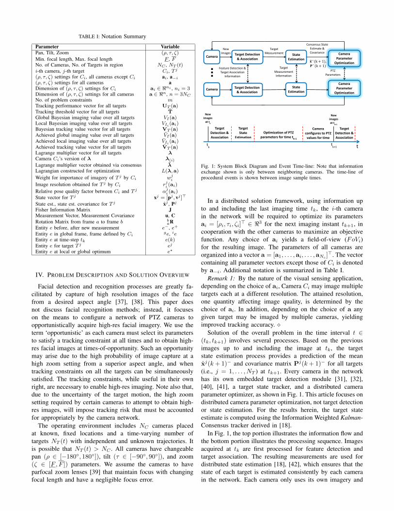
TABLE I: Notation Summary

Parameter VariablePan, Tilt, Zoom (ρ, τ, ζ)Min. focal length, Max. focal length F , FNo. of Cameras, No. of Targets in region NC , NT (t)i-th camera, j-th target Ci, T j

(ρ, τ, ζ) settings for Ci, all cameras except Ci ai, a−i

(ρ, τ, ζ) settings for all cameras aDimension of (ρ, τ, ζ) settings for Ci ai ∈ <ni , ni = 3Dimension of (ρ, τ, ζ) settings for all cameras a ∈ <n, n = 3NC

No. of problem constraints mTracking performance vector for all targets UT (a)Tracking threshold vector for all targets TGlobal Bayesian imaging value over all targets VI(a)Local Bayesian imaging value over all targets VIi (ai)Bayesian tracking value vector for all targets VT (a)Achieved global imaging value over all targets VI(a)Achieved local imaging value over all targets VIi (ai)Achieved tracking value vector for all targets VT (a)Lagrange multiplier vector for all targets λCamera Ci’s version of λ λ(i)

Lagrange multiplier vector obtained via consensus λLagrangian constructed for optimization L(λ,a)

Weight for importance of imagery of T j by Ci wji

Image resolution obtained for T j by Ci rji (ai)

Relative pose quality factor between Ci and T j αji (ai)

State vector for T j xj = [pj , vj ]>

State est., state est. covariance for T j xj , Pj

Fisher Information Matrix JMeasurement Vector, Measurement Covariance u, CRotation Matrix from frame a to frame b b

aREntity e before, after new measurement e−, e+

Entity e in global frame, frame defined by Cige, ie

Entity e at time-step tk e(k)Entity e for target T j ej

Entity e at local or global optimum e∗

IV. PROBLEM DESCRIPTION AND SOLUTION OVERVIEW

Facial detection and recognition processes are greatly fa-cilitated by capture of high resolution images of the facefrom a desired aspect angle [37], [38]. This paper doesnot discuss facial recognition methods; instead, it focuseson the means to configure a network of PTZ cameras toopportunistically acquire high-res facial imagery. We use theterm ‘opportunistic’ as each camera must select its parametersto satisfy a tracking constraint at all times and to obtain high-res facial images at times-of-opportunity. Such an opportunitymay arise due to the high probability of image capture at ahigh zoom setting from a superior aspect angle, and whentracking constraints on all the targets can be simultaneouslysatisfied. The tracking constraints, while useful in their ownright, are necessary to enable high-res imaging. Note also that,due to the uncertainty of the target motion, the high zoomsetting required by certain cameras to attempt to obtain high-res images, will impose tracking risk that must be accountedfor appropriately by the camera network.

The operating environment includes NC cameras placedat known, fixed locations and a time-varying number oftargets NT (t) with independent and unknown trajectories. Itis possible that NT (t) > NC . All cameras have changeablepan (ρ ∈ [−180◦, 180◦]), tilt (τ ∈ [−90◦, 90◦]), and zoom(ζ ∈ [F , F ]) parameters. We assume the cameras to haveparfocal zoom lenses [39] that maintain focus with changingfocal length and have a negligible focus error.

tk t

k+1

Target Detection & Association

Target Detection & Association

t

Target State

Estimation

Camera configures to PTZ

values for time t

New images

at tk

New images at t

k+1

Optimization of PTZ parameters for time t

k+1

Camera Target Detection

& Association

State Estimation

Camera Parameter

Optimization

New Images

Target Measurement

Feature Detection & Target Association

Information

Target Measurement Information

Consensus State Estimate & Covariance

PTZ Parameters

Camera Target Detection

& Association

State Estimation

Camera Parameter

Optimization

𝐱 −(k + 1), 𝐏−(k + 1)

Fig. 1: System Block Diagram and Event Time-line: Note that informationexchange shown is only between neighboring cameras. The time-line ofprocedural events is shown between image sample times.

In a distributed solution framework, using information upto and including the last imaging time tk, the i-th camerain the network will be required to optimize its parametersai = [ρi, τi, ζi]

> ∈ <3 for the next imaging instant tk+1, incooperation with the other cameras to maximize an objectivefunction. Any choice of ai yields a field-of-view (FoVi)for the resulting image. The parameters of all cameras areorganized into a vector a = [a1, . . . ,ai, . . . ,aNc ]>. The vectorcontaining all parameter vectors except those of Ci is denotedby a−i. Additional notation is summarized in Table I.

Remark 1: By the nature of the visual sensing application,depending on the choice of ai, Camera Ci may image multipletargets each at a different resolution. The attained resolution,one quantity affecting image quality, is determined by thechoice of ai. In addition, depending on the choice of a anygiven target may be imaged by multiple cameras, yieldingimproved tracking accuracy. �

Solution of the overall problem in the time interval t ∈(tk, tk+1) involves several processes. Based on the previousimages up to and including the image at tk, the targetstate estimation process provides a prediction of the meanxj(k + 1)− and covariance matrix Pj(k + 1)− for all targets(i.e., j = 1, . . . , NT ) at tk+1. Every camera in the networkhas its own embedded target detection module [31], [32],[40], [41], a target state tracker, and a distributed cameraparameter optimizer, as shown in Fig. 1. This article focuses ondistributed camera parameter optimization, not target detectionor state estimation. For the results herein, the target stateestimate is computed using the Information Weighted Kalman-Consensus tracker derived in [18].

In Fig. 1, the top portion illustrates the information flow andthe bottom portion illustrates the processing sequence. Imagesacquired at tk are first processed for feature detection andtarget association. The resulting measurements are used fordistributed state estimation [18], [42], which ensures that thestate of each target is estimated consistently by each camerain the network. Each camera only uses its own imagery and

data communicated from its neighbors’ on the communicationgraph. Consistency and accuracy of state estimation are pre-requisites that enable distributed optimization of the networkparameter vector a for high-res image acquisition at tk+1.Upon completion of the target state estimation process, a priortarget state estimate g xj(k+1)− and a prior covariance matrixPj(k + 1)− are available for each target T j at the futuresampling time tk+1. Subsequently, each camera will optimizeits PTZ parameter settings ai using g xj(k+1)− and Pj(k+1)−

as inputs. Following computation of an optimal PTZ setting,each camera Ci physically changes its settings to the specifiedvalue ai(tk+1). The focus of this paper is on the algorithmswithin the optimization block as highlighted in Fig. 1.

Remark 2: If cameras take images with a period Ts, thedesigner could choose to re-optimize the camera parametersettings a after every M -th image, resulting in tk = MTs,while still using all M images for target detection and tracking.In this article, we choose to use M = 1. In future work, itcould be interesting to adapt M in response to events.�

Remark 3: It is useful to compare different optimizationapproaches. In centralized optimization, one entity wouldreceive all the required information and adjust the entire vectora to maximize the expected value function. Convergenceof centralized optimization methods are well understood. Indistributed approaches, each agent Ci will only adjust theproposed values of its parameters ai for the next imaging time.In distributed sequential optimization, while Ci is adjustingai, all other cameras Cj for j 6= i are idle. Camerassitting idle potentially save energy at the expense of timeto reach convergence. The convergence of such schemes isstraightforward to analyze as each camera is solving a muchlower dimension optimization problem. The analysis would besimilar to that for the centralized case. In distributed paralleloptimization, all cameras adjust their parameters simultane-ously. Convergence of this case is more complex, requiringresults from optimization and game theory, and cost functionsmeeting certain technical requirements.

V. BACKGROUND

This section briefly reviews concepts of optimization [43]and game theory [36], [44] necessary for the solution method-ology proposed herein.

A. Centralized Constrained Optimization

Consider a standard convex vector optimization (e.g., maxi-mization) problem with a differentiable primal objective func-tion1 fo and differentiable inequality constraints gj

maximize fo(a) (1)subject to gj(a) ≥ 0, j = 1, · · · ,m,

where m is the total number of constraints and a ∈ <n. TheLagrangian L(λ,a) augments the primal objective function

1The notation fo(a) is short for fo(a : xj , j = 1, . . . , NT ), which ismore precise in making explicit the fact that the value depends on the targetstate; however, it is too cumbersome to be effective.

with the constraints

L(λ,a) = fo(a) +

m∑j=1

λjgj(a) = fo(a) + λ>g, (2)

where g is the vector of constraint functions and λ ∈ <m isthe Lagrange multiplier vector with λj ≥ 0.

Since the objective and constraint functionsfo, g1, · · · , gm are differentiable, if an optimum a∗

exists, then the Lagrangian L(λ∗,a∗) attains its maximumat the primal-dual pair (a∗,λ∗) that must satisfy the KKTconditions

∇fo(a∗) +

m∑j=1

λj∗ ∇gj(a∗) = 0, (3)

gj(a∗) ≥ 0, λj∗ ≥ 0, (4)λj∗gj(a∗) = 0. (5)

The KKT conditions provide a certificate for optimality.In a centralized solution approach, the Lagrangian is max-

imized by search over the parameters a and λ. This requiresthat all data and all parameters are available at a centralcontroller. Although, proofs of optimality are simpler and wellknown for this centralized approach, for reasons stated in theintroduction, we are interested in decentralized solutions.

B. Game Theory and Ordinal Potential Functions

For a distributed optimization approach, Ci will only adjustai and λ. A challenge in formulating a distributed optimizationproblem is the decoupling of the system objective into localobjectives, one for each agent. The game theory literature andthe concept of potentiality provides guidance for addressingthis challenge.

Consider a ∈ S and ai, bi ∈ Si, where S = S1×. . .×SNC

is the collection of all possible camera parameter settings inthe game G, and Si is the collection of all possible cameraparameter settings for Ci. The sets S and Si for i = 1 to NC ,referred to as action sets within the game theory literature, arecompact. Let2 φi(ai : a−i) denote the local objective functionof Ci. Game Gp is a potential game if ∃ a potential functionφp : S 7→ < such that ∀a ∈ S and ∀ai,bi ∈ Si,

φp(bi,a−i)− φp(ai,a−i) = φi(bi : a−i)− φi(ai : a−i). (6)

Game Go is an ordinal potential game if ∃ an ordinal potentialfunction φo : S 7→ < such that ∀a ∈ S and ∀ai,bi ∈ Si,

φo(bi,a−i)− φo(ai,a−i) > 0

⇔ φi(bi : a−i) − φi(ai : a−i) > 0. (7)

Potential games and ordinal potential games allow the globalutility maximum to be achieved by maximization of the localutilities of each camera. When Eqn. (7) is satisfied, the localobjective functions are said to be aligned with the globalobjective. Given φo(a), if the local utilities are defined asφi(ai : a−i) = φo(ai,a−i), then it is straightforward to showthat the resulting game is a potential game.

2This notation φi(ai : a−i) means that the value of the function φi maydepend on both ai and a−i, but that ai as treated as an independent variablewhile a−i is treated as a constant by Ci.

Thus, by defining the global objective function as an ordinalpotential function with the individual local camera objectivesaligned to it, the game becomes an ordinal potential game.When the set S is compact, and a game has a continuouspotential function, then the game has at least one Nash Equi-librium. Therefore, given any feasible initial condition, at eachstep for which one camera increases its own utility, the globalobjective function increases correspondingly, due to G beinga potential game. If φo is continuous and S is compact thenφo(a) is bounded above; therefore, the optimization convergestoward a maxima. At the maxima, no camera can achievefurther improvement and thus a Nash equilibrium is reached.

C. Distributed Constrained Optimization

For the distributed approach define the local constrainedoptimization problem for the i-th camera

maximize fi(ai) (8)subject to gj(ai : a−i) ≥ 0, j = 1, · · · ,m,

where ai ∈ <ni , and a−i ∈ <n−ni . The local Lagrangian is

Li(λ,ai : a−i) = fi(ai) +

m∑j=1

λjgj(ai : a−i)

= fi(ai) + λ>g, (9)

where g is the vector constraint and λ ∈ <m with λj ≥ 0.If we define the global objective function as the sum of

local objective functions:

fo(a) =

NC∑i=1

fi(ai), (10)

then from Eqns. (2–5), (9), and (10), ∀a ∈ S, and ∀ai,bi ∈ Si,

L(λ,bi,a−i)− L(λ,ai,a−i) > 0

⇔ Li(λ,bi : a−i)− Li(λ,ai : a−i) > 0, (11)

where the objective of each agent is to maximize its localLagrangian. Therefore, Li and L are aligned, and the globalLagrangian L is an ordinal potential function.

Remark 4: In a potential game, Ci can only choose its ownaction ai, but will take into account the proposed actions a−iof all other agents. The actions of all other agents a−i aredetermined by the other agents. Because Ci is the only agentable to select ai, consensus between agents is inappropriatefor computation of ai. Instead, a modified flooding approachwill be used, see Section VIII-B. At the same time, all camerasmust collaboratively choose actions and λ to ensure that allconstraints are satisfied. During distributed optimization eachCi has a local version of the Lagrange multiplier vector,denoted as λ(i). A consensus algorithm is used to ensure theconvergence of λ(i) to a single value, see Section VIII-C.�

VI. SYSTEM MODEL

The continuous-time state space model of target T j is:

xj(t) = F xj(t) + G ωj(t) (12)

where j = 1, . . . , NT is the target number and xj = [gpj ; gvj ]with gpj and gvj representing the position and velocityvectors in the global (earth) frame. The process noise vectorωj ∈ <3 is assumed to be zero mean Gaussian with powerspectral density Q. The discrete-time equivalent model is:

xj(k + 1) = Φxj(k) + γ(k) (13)

where Φ = eFT is the state transition matrix, γ ∼ N (0,Qd)is the process noise, and T = tk+1−tk is the sampling period.

A. State Estimate Time Propagation

The state estimate and its error covariance matrix arepropagated between sampling instants using [45]:

xj(k + 1)− = Φxj(k)+ (14)Pj(k + 1)− = ΦPj(k)+Φ> + Qd. (15)

B. Camera Coordinate Transformations

Target T j’s position in the i-th camera’s frame, cipj , isrelated to its position in the global frame gpj by:

gpj = gciR

cipj + gpci (16)cipj = ci

g R[gpj − gpci ], (17)

where gpci is the position of Ci in global frame and cig R is

a rotation matrix that is a function of the camera mountingangle and ai.

C. Measurement Model

Camera measurement models are derived in various refer-ences [32], [46]. The following presents final results only forthe expressions needed in this article. The derivation in [32]uses a notation similar to that herein.

Let the coordinates of target T j in camera Ci’s frame becipj =

[cixj , ciyj , cizj

]>. The standard pin-hole perspective

projection camera model for Ci and T j , assuming that T j isin the FoV of camera Ci is,

iiuj =

Fisx

cixj

cizj+ ox

Fisy

ciyj

cizj+ oy

+ iiηj , (18)

where sx and sy give the effective size of a pixel in (m/pixel)measured in the horizontal and vertical directions, respectively;Fi is the focal length setting defined by ai; the point (ox, oy)gives the coordinates of the image plane center in pixels; andthe measurement noise iiηj ∼ N (0,Cji ) with Cji (ai) ∈ <2×2.The fact that the measurement noise covariance Cji is depen-dent on ai is important. Note, for example, that as the focallength increases, the size of a target in the image increasesand the pixel uncertainty of its location changes.

Given the estimated state and the camera model, the pre-dicted measurement is

ii uj =

Fisx

ci xj

ci zj+ ox

Fisy

ci yj

ci zj+ oy

. (19)

The measurement residual ii uj isii uj = iiuj − ii uj . (20)

D. Observation Matrix Hji

The linearized relationship between the residual and theposition error vector is

iiuj − ii uj ≈ Hji

(gpj −g pj

), (21)

where Hji =

∂iiuj

∂gpj

∣∣∣∣g pj

∈ <2×3 is defined in [34]. Note that

Hji is a function of both gpj and ai. When T j is not in FoVi,

then Hji = 0 ∈ <2×3.

E. Measurement Update

Using Hji and Eqn. (20), a measurement update for the

state estimates and error covariances for targets in the area isperformed using the Information-Consensus Filter from [18].

VII. IMAGE OPTIMIZATION METHODOLOGY

The goal is to track all targets at all times to a specifiedaccuracy T, to discover times-of-opportunity at which im-proved imagery is obtainable, and to determine the sequenceof PTZ parameters for each camera to achieve these goals.Improved imagery means that the system should only attemptto acquire a high-res image of any target T j at the nextimaging instant if that image is expected to yield higherimaging value for that target than is already available. Themethod implements distributed, simultaneous optimization byall agents to compute the optimal camera parameters a∗relative to Eqn. (1) at each imaging time-instant.

This section starts with specification of the global objectiveand constraints that are subsequently decoupled into localobjectives for each camera. The global objective functionfor the constrained optimization problem is designed as aBayesian imaging value function that accounts for the risk inimaging the target. Risk will be formulated using the Fisherinformation matrix defined as Jj(k+1)− =

(Pj(k + 1)−

)−1.

The prior covariance matrix Pj(k+1)− computed using Eqn.(15) can be written in block form as3:

Pj− =

[Pj−pp Pj−pvPj−vp Pj−vv

], (22)

where Pj−pp is the prior, position error-covariance matrix.

A. Global Imaging Value Function

This section discusses the design and desired properties ofthe global imaging value function VI

(a : gpj−,Pj−

pp

)and the

global constraint set. The notation VI(a : gpj−,Pj−

pp

)with

j = 1, · · · , NT makes explicit that the optimization variable isa, while the value also depends on the distribution of target T j

which is parameterized by(gpj−,Pj−

pp

). For ease of notation,

from this point in the paper, we will drop dependence of VI (a)on gpj− and Pj−

pp, unless needed for clarity.

3The time argument (k + 1) is dropped for ease of notation.

1) Value Function Properties: The imaging value functionshould have the following properties:Continuously differentiable: This is necessary for proofs ofconvergence, and greatly facilitates numeric optimization.Increases with image quality: Herein, image quality isdefined by two parameters: image resolution and relative posebetween the imaging camera and the imaged target.

Image resolution rji (ai,gpj), which is a positive real num-

ber, will be quantified by the number of pixels occupied byT j on camera Ci’s image plane. Given gpj , the resolutionincreases monotonically with zoom ζ of the imaging camera.

Relative pose between camera Ci and target T j will bequantified by the scalar quality factor αji (ai). Let vector ovjbe the target’s velocity vector. Define the vector oCi

to be thei-th camera’s optical axis direction in the global frame

oCi= g

ciRcie3, (23)

where e3 = [0, 0, 1]>. Define oT j to be the vector fromcamera Ci’s position to target T j’s estimated position. Usingthe vectors ovj , oCi

, and oT j we define the scalars

oc =oCi· oT j

‖ oCi‖‖ oT j ‖

, and oo =oCi· ovj

‖ oCi‖‖ ovj ‖

. (24)

The scalar oc ∈ [−1, 1] yields the maximum possible positivevalue of 1 if camera Ci images target T j such that T j is atthe center of its FoV. The scalar oo ∈ [−1, 1] has maximummagnitude when T j’s motion vector ovj is pointing directlytoward or away from camera Ci.

To define αji (ai), we use the following assumption.Assumption 1: (Facial Direction) Target T j faces in the

direction indicated by vector ovj .From Assumption 1 and Eqn. (24), when the scalar oo < 0,

T j is likely to be facing camera Ci. This condition differen-tiates between targets facing Ci and those facing away fromit. The relative pose quality factor is thus defined as

αji (ai) =

{(oc oo)

2 if oo < 00 otherwise.

(25)

Hence when αji ∈ [0, 1] is large, it is likely that T j is facingCi and at the center of Ci’s FoV. The imaging value obtainedby camera Ci for imaging T j located at gpj is defined as

V jIi(ai,gpj) = rji (ai) α

ji (ai). (26)

Balanced Risk: Risk is defined as the probability that thetarget is outside of the FoV of the cameras that are expected toimage it. Risk increases monotonically with zoom ζ, becausethe ground-plane area within the FoV decreases as ζ increases.Herein, we will address risk by using the expected value ofthe tracking constraints and the imaging value.

To understand the issues involved, it is informative to brieflyconsider the simple case where NT = 1 and α1

i > 0 fori = 1, . . . , NC . For this case, if risk was neglected and VI wasdefined with the properties mentioned above, then each camerawould maximize its focal length and select its pan and tiltparameters to center on the expected target location. If instead,the value accounted appropriately for risk, then one or morecamera might significantly increase its zoom parameter, whileat least one of the remaining cameras would use lower zoom

Fig. 2: Non-convexity of the Bayesian Imaging Value Function: The figureis a plot of an example Bayesian imaging value function that highlights themultimodal nature of the function for scenarios where NT > 1.

parameters, to decrease the tracking risk due to the uncertaintyin the estimated target position. The camera at the highestzoom setting would be the one at the best aspect angle.

Remark 5: Fig. 2 depicts the appearance of an exampleBayesian Imaging Value function for a scenario with NT = 2targets in an area monitored by NC = 1 camera. As shown inthe figure, when NT > 1, the summation of the per targetexpected imaging value across the targets for any camerawill typically yield a multimodal (i.e., nonconvex) objectivefunction. Given the expected target positions and their respec-tive distributions, for a constant tilt angle τ , the plot showshow the value of the objective function changes versus zoom(ζ ∈ [ζ, ζ]), and pan angle (ρ ∈ [ρ, ρ]), It can be seen that themulti-modal nature of the function is exaggerated for highervalues of ζ. Thus, the possibility of multiple targets makes thevisual sensing problem inherently non-convex and provideschallenges in achieving optimal solutions. Non-convexity isfurther discussed in Section IX.�

2) Imaging Value VI(a : gpj−,Pj−pp): We define the global

Bayesian image value function as

VI(a) =

NC∑i=1

NT (t)∑j=1

wji (t) E⟨V jIi(ai,

gpj)⟩

(27)

=

NC∑i=1

∫FoVi

NT (t)∑j=1

wji (t) VjIi

(ai, z) ppj (z)

dz,

where wji (t) is a time-varying local dynamic imaging weightthat magnifies the importance of imaging certain targets rela-tive to other targets4. Given the assumptions herein, the prob-ability distribution ppj (z) of the position of T j in the globalframe at the next imaging instant is the Normal distribution

4Specification of wji (t) is application dependent. It could be constant,

user-specified, or could increase as the target approaches a specified locationsuch as an exit. See the example in eqn. (49).

N (gpj−,Pj−pp). The dummy variable z representing targetposition is used for integration over the ground plane, wherethe region of integration is the i-th camera’s FoV.

Each camera integrates over its own FoV. The integral ofimage quality over FoVi as a function of probability weightedtarget position yields the Bayesian value function, whichprovides the desired tradeoff between image quality and risk.

3) Performance Constraints: The performance constraintswill be defined as a function of the posterior Fisher Informa-tion Matrix Jj+

(a : gpj−,Pj−

pp

).

Fisher Information: The Fisher Information Jj for T j inblock form is

Jj =

[Jjpp JjpvJjvp Jjvv

], (28)

where, Jjpp represents the position information matrix. Theposterior position information matrix Jj+pp is given by

Jj+pp = Jj−pp +

NC∑i=1

Hj>

i

(Cji)−1

Hji , (29)

where, Jj−pp is the prior information about T j . As was shownin Section VI-D, Hj

i and Cji are functions of ai and Hji is

a function of the target position. Therefore, Jj+pp depends ona and on the target position. Computation of the expectedtracking accuracy should account for this variation and for theprobability that T j ∈ FoVi.Tracking Performance: We define a vector Uj

T (a :gpj−,Pj−

pp) as a measure of tracking performance for eachtarget in the area. One example is Uj

T (a) = diag(Jj+pp).

Because the quantity UjT (a) depends on whether T j is within

the FoV of each camera that is expected to image it, wedefine the global Bayesian tracking value vector Vj

T (a) asthe expected value of the tracking performance vector Uj

T (a)over the position of T j computed across all the camera’s FoVs:

VjT (a) = Epj

⟨UjT (a)

⟩=

∫ (UjT (a) ppj (z)

)dz, (30)

where all variables are as defined in Eqn. (27) and thesummation over all cameras is accounted for already in eqn.(29), which also accounts for prior information.Tracking Constraint: Each target’s tracking constraint is

VjT (a) � Tj , (31)

where Tj is the user specified lower bound on the trackinginformation about target T j . Due to the reciprocal relationbetween (scalar) information and covariance, the reciprocalof Tj is the upper bound on the covariance of target T j’sstate estimate. The tracking performance threshold Tj is hencemeasured in m−2. The notation ‘�’ in Eqn. (31) indicates aper-element vector inequality. Stacking the Bayesian trackingvalue vectors for each target, we obtain

VT (a) =[V1T , · · · ,V

jT , · · · ,V

NT

T

]>, (32)

and rewrite Eqn. (31) for all targets presently in the area as:

VT (a) � T, (33)

where VT (a), T,0 ∈ <m with m = NT (t)dim(gpj). Eqn.(33) is the global tracking constraint.

4) Global Problem Summary: The constrained global imag-ing value maximization problem can be written as

maximize VI(a : gpj−, Pj−

pp

)(34)

subject to[VT

(a : gpj−, Pj−

pp

)− T

]� 0.

The global Lagrangian L(λ,a) is

L(λ,a) = VI (a) + λ>[VT (a)− T

], (35)

where L : (λ,a) 7→ <, and λ ∈ <m is the Lagrange multipliervector. Thus, to find the optimal primal-dual pair of solutions(a∗,λ∗) through a central controller, the global unconstrainedproblem given by the Lagrangian in Eqn. (35) would be solved.

B. Decoupling the Global Problem

Due to the desired distributed nature of our solution, weneed to decompose the global problem into smaller localproblems that are solvable by each camera.

In our problem formulation, we allow camera Ci to op-timize only its own camera parameter settings ai. Using thissystem restriction, we define the local Bayesian imaging valuefunction for Ci as

VIi(ai) =

∫FoVi

NT (t)∑j=1

(wji (t) V

jIi

(ai, z) ppj (z))dz. (36)

Define VTi(ai) = VT (ai : a−i). This notation con-

cisely indicates that Ci can only alter ai, where for thepurpose of its local optimization a−i is fixed. Note thatVT (ai : a−i) is distinct from VT (ai,a−i) = VT (a) andthat maxai∈Si

VTi(ai) ≤ maxa∈S VT (a). Each agent will

have the constraint VT (ai : a−i) � T. While Ci is changingai, the other agents are simultaneously changing their subvectors of a−i and all agents are broadcasting their currentlocally optimal values through the network. Thus the trackingconstraint for camera Ci is

VTi(ai) � T. (37)

Note that,

VTi(ai) � T ⇔ VjTi

(ai) � Tj for j = 1, . . . , NT (t).

The Fisher Information given in Eqn. (29) can be reorga-nized as:

Jj+pp =

[Jj−pp + Hj>

−i

(Cj−i

)−1

Hj−i

]+ Hj>

i

(Cji)−1

Hji .

For the process of Ci optimizing its parameter vector ai,the contribution from prior information and all other cameras(term in brackets) is independent of ai and considered by Ci

to be constant and known. The term[

Hj>

−i

(Cj−i

)−1

Hj−i

]is computed from a−i which will be available through thedistributed optimization process discussed in Section VIII.

Thus from Eqns. (29-30), we can write

Epj

⟨diag

(Jji

)⟩� T− Epj

⟨diag

(Jj−pp + Jj−i

)⟩, (38)

where Jji = Hj>

i

(Cji)−1

Hji and Jj−i = Hj>

−i

(Cj−i

)−1

Hj−i.

The right hand side of this inequality represents, for the current

proposed settings of the other cameras a−i, the expected im-provement in tracking accuracy required from Ci for imagingT j to have a feasible global solution. Targets for which theright-hand side of Eqn. (38) is negative can be removed fromthe set of tracking constraints for Ci.

From Eqns. (36) and (37), the local imaging value maxi-mization problem can be written as

maximize VIi(ai : gpj−, Pj−

pp

)(39)

subject to VTi

(ai : a−i,

gpj−, Pj−pp

)� T.

The local Lagrangian Li(λ(i),ai) is

Li(λ(i),ai

)= VIi(ai) + λ>(i)

[VTi

(ai)− T]. (40)

Thus, for camera Ci to find its local optimal primal-dual pairof solutions (a∗i ,λ

∗(i)), Ci will maximize the local uncon-

strained Lagrangian given in Eqn. (40).In this approach, all cameras in the network optimize

simultaneously. The subscript (i) on λ(i) in Eqn. (40) indicatesthat the Lagrange multiplier vector picked by camera Ci tosolve the problem is a local variable and may not be globallythe same throughout the network. In order to overcome thispredicament, cameras in the network employ a variant of thealgorithm described in [47], [48] to perform dynamic averageconsensus over the local Lagrange multiplier vectors. Thisresults in a consensus-step after each optimization-step Thealgorithm is explained in detail in Section VIII.

C. Lagrangian as an Ordinal Potential Function

For the problem stated in Eqn. (34), note that the globalobjective of the multi-camera network defined in Eqn. (27) isthe sum over the local objectives defined in Eqn. (36)

VI(a) =

NC∑i=1

VIi(ai). (41)

At each optimization step κ, the i-th camera adjusts λ(i)(κ)and ai(κ), leaving a−i(κ) fixed, to solve the problem inEqn. (39) with VIi(ai) defined in Eqn. (36). Dynamic averageconsensus over λ(i) between optimization steps forces eachagent’s local value toward a non-negative consensus agreementvector λ(κ) = 1

Nc

∑i λ(i)(κ). Convergence of the dynamic

game is assured when the local Lagrangians Li(λ(i),ai), andthe global Lagrangian L(λ,a) form an ordinal potential game.

From Eqns. (35), (40),and (41), ∀λb, λa � 0, let L =L(λb, bi, a−i)− L(λa, ai, a−i). Thus,

L =

NC∑i=1

VIi(bi) + λ>b[VT (bi, a−i)− T

]−

NC∑i=1

VIi(ai)− λ>a[VT (ai, a−i)− T

]= VIi(bi) +

∑l 6=i

VIl(al) + λ>b[VT (bi, a−i)− T

]−VIi(ai)−

∑l 6=i

VIl(al)− λ>a[VT (ai, a−i)− T

]= Li(λb, bi : a−i)− Li(λa, ai : a−i).

Hence, ∀a ∈ S, ∀ai,bi ∈ Si, and ∀λb, λa � 0,

L(λb, bi, a−i)− L(λa, ai, a−i) > 0

⇔ Li(λb, bi : a−i)− Li(λa, ai : a−i) > 0.

Therefore, as explained in Sections V-B and V-C, Eqns. (35)and (40) form an ordinal potential game.

VIII. DISTRIBUTED OPTIMIZATION

The distributed optimization process can be broken downinto three separate steps, where κ denotes the iteration counter:

1) Camera Parameter Optimization: Each cameraCi computes (ai,λ(i)) to increase Li

(λ(i),ai : a−i

)while holding a−i constant. It then communicatesthe newly computed local primal-dual pair estimates(i, κ,ai(κ),λ(i)(κ)

)and new portions of a−i to its

neighbors Ni.2) Camera Parameter Replacement: Each camera Cn

that is a neighbor of Ci (i.e. Cn ∈ Ni) receives(i, κ,ai(κ),λ(i)(κ),a−i

). It replaces its previous value

of (ai,a−i) using the rules of replacement described inSection VIII-B.

3) Consensus on Lagrange Multipliers: Ci performsdynamic average consensus on its local Lagrange multi-plier vector λ(i)(κ) and the Lagrange multiplier vectorsreceived from cameras in Ni to converge towards a con-sensus Lagrange multiplier vector λ, using the Lagrangemultiplier update law in Eqn. (43), defined in SectionVIII-C.

This distributed optimization process is then iterated over κuntil a stopping criteria is achieved.

Since the optimization problem described by Eqn. (39) isnon-convex, any solution found may only be locally optimal.It is assumed that all agents start with identical values of a(κ)for κ = 0 and that a(0) is not on the separatrix dividing thedomain of attraction of one local optimum from another.

A. Connectivity, Communication, and Consensus

The approach requires the following standard assumptionson the camera communication graph.

Assumption 2: (Connectivity) The camera communicationgraph is undirected, and connected, i.e. there exists at leastone communication path from each agent to every other agentin the network.

Remark 6: In [48], each agent changes λ and the entirevector a while computing a dual solution, then using consensuson both a and λ. Herein, agent Ci only optimizes λ and ai,which is a subvector of a. When the subvector ai is broadcastto the neighbors of Ci, they pass it to their neighbors. Eachagent receiving a newer value of ai replaces their older value.Thus, for the approach herein, each camera Ci need onlyperform dynamic average consensus on λ(i) and the set ofLagrange multiplier vectors {λ(n)} for Cn ∈ Ni. Connectivityensures that the changes to ai and λ(i) by each Ci eventuallyaffect all agents in the network. The convergence of consensusis asymptotic, but becomes trivial for strictly feasible solutions,which have λ = 0. The effects of a change in any ai are fully

distributed throughout the network in a finite number of steps,which is less than the diameter of the network.�

Assumption 3: (Weights Rule) There exists a scalar β > 0such that for each i ∈ [1, Nc], ωii(κ) ≥ β, and ωin(κ) ∈ [β, 1]for Cn ∈ Ni. If cameras Ci and Cn are not directly connected,then ωin(κ) = 0.

Assumption 4: (Double Stochasticity) Let Bi = Ci⋃Ni,

and∑l∈Bi

ωil(κ) = 1 and∑i∈Bi

ωil(κ) = 1.Assumption 3 ensures that all cameras are influential [47]

while performing consensus on the local Lagrange multipliervectors, and Assumption 4 ensures that all cameras asymp-totically converge to a consensus Lagrange multiplier vectorλ � 0 [49].

B. Camera Parameter Replacement Rule

We use a variant of the flooding algorithm [50] topropagate the local variables through the network of cam-eras. After Ci computes ai(κ), it delivers the information{i, κ,ai(κ),λ(i)(κ)} to its neighbors Ni, and will rebroadcastto its neighbors any updated PTZ information, {l,al, κl}for l 6= i, that it received since the last broadcast. Usingrebroadcast, each agent’s parameter updates travel throughouta connected network exactly one time. For the l-th subvectorin C ′is version of a, Ci has a value al(κl) and a time-stamp κl both computed by Cl, even if Ci and Cl are notneighbors. Because the network may contain loops, Ci mayreceive information about other cameras via multiple paths. Ciwill replace its l-th subvector with the received informationonly if the time-stamp in {l,al, κl} is more recent than thetime stamp corresponding to the value it is currently using.Otherwise, the message is discarded without rebroadcast.

C. Distributed Lagrangian Consensus

At iteration κ camera Ci receives the set of Lagrangemultiplier vectors {λ(n)(κ)} for Cn ∈ Ni. It also has its localcopy of a. Its local computations must jointly optimize ai andλ (given a−i) while also converging toward agreement acrossthe network on the value of λ. This section describes dynamicaverage consensus on the local versions of Lagrange multipliervectors. Following the notation in [48], we refer to this as adistributed Lagrangian consensus algorithm.

Camera Ci iteratively optimizes using the update law [47]:

ai(κ+ 1) = −s(κ) Da(i)(κ) (42)

λi(κ+ 1) = νλ(i)(κ)− s(κ) Dλ(i)

(κ), (43)

where the scalar s(κ) > 0 is the step-size,

Dai= ∇ai

Li(λ(i)(κ), ai(κ) : a−i(κ)

),

and

Dλ(i)= ∇λ(i)

Li(λ(i)(κ), ai(κ) : a−i(κ)

)=

[VTi

(a∗i )− T].

The first term in Eqn. (43) is the consensus term, which is aconvex combination of λ(i)(κ) and {λ(n)(κ)}:

νλ(i)(κ) =

∑l∈Bi

ωil(κ) λ(l)(κ), (44)

which always yields νλ(i)(κ) ∈ <m as a non-negative vector.

The second term is the gradient descent term, which adjustsλ(i) in a coordinated fashion with the change in ai to convergetoward an optimal and feasible solution relative to the localoptimization problem. The step-size s(κ) > 0 can be adjustedto maintain component-wise non-negativity of λ(i).

With Assumptions 2, 3 and 4 , it is shown in [47]–[49]that for all i = 1, . . . , NC , there exist λ � 0 such thatlimκ→∞ ‖λ− λ(i)(κ)‖ = 0.

D. Certificate for Optimality

For the unconstrained maximization problem defined byEqn. (40) for each agent, the optimal primal-dual pair(a∗i ,λ

∗(i)

)must satisfy the KKT conditions:

∇VIi(a∗i ) + [∇VTi(a∗i )]

>λ∗(i) = 0, (45)

VTi(a∗i )− T � 0, λ∗(i) � 0, (46)

λ∗>(i)[VTi

(a∗i )− T]

= 0, (47)

which provide a certificate of optimality at each agent.All cameras optimize in parallel. Camera Ci broadcasts

a∗i and λ∗(i), and new portions of a−i, to its neighbors whopropagate them through the network. While Ci is locallyoptimizing its settings, it is accounting for an updated λ(i),and for each target, the prior information Jj− and expectednew information based on the currently best settings of all theother cameras a−i.

Optimization stops when either an optimum is achieved, auser-defined stopping condition is met, or the time intervalallotted for optimization elapses (see Fig 1). The solutionapproach described in [32] optimized a weighted combinationof tracking and imaging; whether or not an optimum wasachieved, there was no guarantee that the tracking specificationwas achieved. For the approach herein, the KKT conditionsdescribed in Eqns. (45 - 47) provide a certificate on optimalityand feasibility (i.e., satisfaction of the tracking specification).Numeric algorithms to solve the constrained optimizationproblem defined in Eqn. (39), to which the KKT conditions ofEqns. (45–47) apply, first find a feasible solution, then searchwithin the feasible set for the optimal feasible solution. Thus,when the time interval allotted for optimization elapses, even ifthe solution is sub-optimal, the solution obtained is guaranteedto be feasible. This results in all targets being tracked to thespecified tracking accuracy at all times, while procuring high-res imagery when opportunity arises. After optimization, thecameras physically alter their settings to the optimal values inreadiness for upcoming images at tk+1.

Thus, by using the replacement step in Section VIII-B andthe Lagrange multiplier update law from Eqn. (43), at eachconsensus iteration κ, every camera maintains an estimate ofthe primal-dual pairs of all cameras.

IX. IMPLEMENTATION

This section describes a Matlab implementation of theproposed approach. The goal of the simulation is to evaluatethe performance of a distributed PTZ camera network usingthe methods described herein to obtain opportunistic high-res

0 2 4 6 8 10 12 14 16 18 20

0

2

4

6

8

10

12

14

16

18

20

x-position in global frame

y-positionin

globalframe

Top View of Camera Parameter OptimizationgpC1

gpC2

gpC3

FoV1

FoV2

FoV3

Entry

Exit

Fig. 3: Top-view of 20× 20 surveillance area at t = 0, prior to target entry.Camera locations are indicated by colored stars. The camera’s FoV boundaryis drawn on the ground plane using the same color as its star. The FoV ofthe camera is the convex area interior of this polygon.

facial imagery of targets moving in a region, while trackingall targets at all times to a specified tracking accuracy.

A. Scenario, Setup and Experiment Details

Fig. 3, shows a 400 m2 area being monitored by NC =3 calibrated cameras located at C1 = [10, 0, 3]>, C2 =[0, 10, 3]>, and C3 = [20, 10, 3]>m. Camera locations areindicated by colored stars. The boundary of the FoV for eachcamera is drawn as a wide solid line in a color coordinatedwith the color of the position marker of the camera. Note thatthe FoV is the area in the interior of this polygon.

Every target T j is modeled as a circular disc of negligibleheight and a radius of 30 cm. All target discs are coplanarto the ground plane. The entrance to the area is located aty = 20, x ∈ [1, 3] and indicated by the pink hash marks inFig. 3. Targets enter through the entrance at random times;therefore, the total number of targets in the area is time variant.When a target T j enters the area, its position coordinates arerandomly initialized in [gxj , gyj , 0]>, where gxj ∈ [1, 3] andgyj = 20. When a new target is detected, the number oftargets NT (t) is increased, and the target state is augmentedto the state vector and included in the imaging and trackingvalue functions. The maximum number of targets permissiblein the area was limited such that 0 ≤ NT (t) ≤ NT whereNT = 10. To ensure that targets entering the area are detected,the entrance must be constantly monitored. This is achievedby inserting an artificial stationary target at (2, 20, 0) withconstant position uncertainty of 2m2. Once a target is in theroom, its motion is generated using the model in Eqn. (13).The exit to the room is located at y = 0, x ∈ [5, 10] andindicated by the black hash marks in Fig. 3. If the targettrajectory intersects the wall in this region, then the targethas exited the room, in which case, the target state is removedfrom the state vector, excluded from the imaging and trackingvalue functions, and the number of targets NT (t) is decreased.

5 10 15 20 25 3010

0

101

102

Simulation Time

VT(a)

a. Expected Bayesian Tracking Value for each target

V1T (a)

V2T (a)

V3T (a)

V4T (a)

V5T (a)

V6T (a)

V7T (a)

V8T (a)

V9T (a)

V10T (a)

T

5 10 15 20 25 3010

0

101

102

Simulation Time

VT(a)

b. Achieved Bayesian Tracking Value for each target

V1

T (a)

V2

T (a)

V3

T (a)

V4

T (a)

V5

T (a)

V6

T (a)

V7

T (a)

V8

T (a)

V9

T (a)

V10

T (a)

T

5 10 15 20 25 3010

0

102

104

106

Simulation Time

VI(a)

c. Achieved Imaging Value

V I(a)

V I1(a1)

V I2(a2)

V I3(a3)

5 10 15 20 25 30

−80

−60

−40

−20

0

20

40

60

80

Panρ◦

∗i

Simulation Time

d. Optimal Pan Angles

5 10 15 20 25 30

−80

−60

−40

−20

0

20

40

60

80

Tiltτ◦

∗i

Simulation Time

e. Optimal Tilt Angles

5 10 15 20 25 30

1

2

3

4

5

6

7

8

9

10

Zoom

ζ∗

i

Simulation Time

f. Optimal Zoom Values

ρ1

ρ2

ρ3

τ1τ2τ3

ζ1

ζ2

ζ3

Distributed Constrained Optimization for Bayesian Opportunistic Visual Sensing

Fig. 4: Bayesian Tracking and Imaging Values: Fig. a (top left) shows that the camera network expects to successfully and co-operatively satisfy the trackingconstraint T = 1.0 m−2 for every target, at all times. Fig. b (middle left) shows that the achieved tracking values satisfy the tracking constraint T. Fig. c(bottom left), plots the achieved local imaging value VIi (ai) and the achieved global imaging value VI(a) (i.e., sum of the local values). Figs. d (top right),e (middle right) and f (bottom right) show the per camera optimal pan angle ρ◦ ∗i , tilt angle τ◦ ∗i and zoom ζ ∗i values, respectively.

Remark 7: Note that the target trajectory from Eqn. (13) mayintersect a wall. If the point of intersection is the exit, then the targetexits the area as described above. If the point of intersection is notthe exit, then the target trajectory reflects off the wall.�

As discussed in Section VI-C, the measurement modeldepends on the camera parameters. In addition, while theimage processing algorithms may compute the centroid ofthe feature region in the image plane to subpixel resolution,the covariance matrix used in the state estimation routinemust account for the the uncertainty in the computed centroidrelative to the “actual target centroid.” Let nji (ai) represent thearea occupied by T j’s image on Ci’s image plane measured insq. pixels. For this simulation, the estimation routine modelsthe covariance of the measurement of T j by Ci as

Cji (ai) =

nji (ai)

piσ2x 0

0nji (ai)

piσ2y

, (48)

where pi is the pixel resolution of Ci’s image plane (in sq.pixels) and σ2

x and σ2y (in sq. pixels) are positive constants. For

this simulation, each camera Ci was set to an image resolutionpi of 800× 600 sq. pixels, with σx = σy = 5 pixels.

The results in Figs. 4 - 6 correspond to a 31 sec. simulation.

All cameras image at a frequency of 1 Hz, with the firstimages obtained at time t = 1 second.

All cameras optimize simultaneously, using an interior-point method [51]. The tracking constraint in Eqn. (37) usesT = 1.0 m−2. Ci receives camera parameters a∗−i through itsneighbors, and uses its current parameters ai to implement themethod described in Section VIII.

Define V jIi to be the imaging value achieved by camera Cifor imaging T j . The weight wji (t), in Eqn. (27), is defined asthe continuously differentiable and bounded function:

wji (t) = σd(dj(t)

)σv

(V j , V jIi(t)

), (49)

where σd = 1 + 11+exp[lddj(t)] , and σv = 1

1+exp[lv(V j−V jIi

(t))].

The symbol V j = maxτ<t, i∈[1,Nc]

(V jIi(τ)

)is the best image

quality for target T j for any camera and any prior image. Thesymbol dj(t) is the distant between T j’s estimated position attime t and the exit. With these definitions σd(t) ∈ [1, 2] andσv(t) ∈ [0, 1]. This definition of wji (t) gives higher value (i.e.,emphasizes) those targets nearest to the exit and those targetsfor which the value of the next image is expected to improvethe most relative to prior imagery.

0 2 4 6 8 10 12 14 16 18 20

0

2

4

6

8

10

12

14

16

18

20

x-position in global frame

y-positionin

globalframe

Top View of Camera Parameter Optimization gpC1

gpC2

gpC3

FoV1

FoV2

FoV3

gpj

gpj+

Entry

Exit

(a) Optimized FoVs at t = 1.

0 2 4 6 8 10 12 14 16 18 20

0

2

4

6

8

10

12

14

16

18

20

x-position in global frame

y-positionin

globalframe

Top View of Camera Parameter Optimization gpC1

gpC2

gpC3

FoV1

FoV2

FoV3

gpj

gpj+

Entry

Exit

(b) Optimized FoVs at t = 21.

0 2 4 6 8 10 12 14 16 18 20

0

2

4

6

8

10

12

14

16

18

20

x-position in global frame

y-positionin

globalframe

Top View of Camera Parameter Optimization gpC1

gpC2

gpC3

FoV1

FoV2

FoV3

gpj

gpj+

Entry

Exit

(c) Optimized FoVs at t = 24.

0 2 4 6 8 10 12 14 16 18 20

0

2

4

6

8

10

12

14

16

18

20

x-position in global frame

y-positionin

globalframe

Top View of Camera Parameter Optimization gpC1

gpC2

gpC3

FoV1

FoV2

FoV3

gpj

gpj+

Entry

Exit

(d) Optimized FoVs at t = 25.

0 2 4 6 8 10 12 14 16 18 20

0

2

4

6

8

10

12

14

16

18

20

x-position in global frame

y-positionin

globalframe

Top View of Camera Parameter Optimization gpC1

gpC2

gpC3

FoV1

FoV2

FoV3

gpj

gpj+

Entry

Exit

(e) Optimized FoVs at t = 30.

5 10 15 20 25 3010

0

101

102

103

104

105

106

107

Simulation Time

GlobalBayesianIm

agingValueper

Target

Vj I(a)

Opportunistic High-res Facial Capture per Target

V 1I (a)

V 2I (a)

V 3I (a)

V 4I (a)

V 5I (a)

V 6I (a)

V 7I (a)

V 8I (a)

V 9I (a)

V 10I (a)

(f) Opportunistic Hi-res Capture.

Fig. 5: Top-view of Opportunistic High-res Facial Image Capture: Figs. a (top left), b (top center), c (top right), d (bottom left), and e (bottom center) showthe optimized FoVs at times of opportunity: t = 1, t = 21, t = 24, t = 25 and t = 30, respectively. Each figure shows the optimized FoVs of the camerasafter feasible optimal solutions are achieved. Fig. f (bottom right) shows the expected per target imaging value V j

I

(a(t)

)from Eqn. (50).

B. Single Trial Results

For this simulation, targets T 1 to T 10 entered the area attimes 0.1, 10.2, 11.1, 14.2, 20.4, 22.9, 27.2, 28.8, 30.1,and 30.4 seconds, respectively. Target T 1 left the area at time14.4 seconds. No other targets left the area. When T j enters,a camera monitoring the entrance images it, detects the newtarget and augments it to its state vector. Other cameras addthe new target to their state vector as they receive the newtarget information at the state estimation stage.

1) Bayesian Imaging and Tracking Performance: Camerasmaximize their local Lagrangians Li(λ∗(i),a

∗i ) to satisfy the

tracking spec and maximize their local Bayesian imagingvalues. Fig. 4a shows that the expected Bayesian trackingvalue Vj

T (a∗) is greater than the tracking spec, at all times;therefore, all primal-dual solutions (a∗i ,λ

∗(i)) obtained through

local optimization are expected to be feasible at all imaginginstants. Because the solutions are strictly feasible, using Eqn.(47), it is trivial to prove that the dual optimal Lagrangemultiplier vectors for all cameras are λ∗(i)(t) = λ = 0 ∈ <m,where m = 2NT (t).

The proposed approach utilizes predicted target motionbased on state estimates from the last imaging time. Estimationerror or unexpected maneuvers by targets, such as a simulatedtarget reflecting of a wall, can lead to a drop in the accuracyactually achieved. Fig. 4b shows the tracking value Vj

T (a∗)actually achieved by the network. Various instances of dif-ferences between the expected and achieved accuracy can beobserved through the simulation time. Since the target motion

is a random process, there is no deterministic guarantee thatthe achieved accuracy meets the specification.

Fig. 4c shows the achieved imaging values of each cameraand of the network of cameras. The peak values occur at thoseopportunistic times at which the cameras procure high-resfacial images of targets, while the tracking constraints on alltargets are satisfied. A high value for VIi (a∗i ) indicates a high-res facial capture by camera Ci. Given the target trajectories ofthis simulation, all cameras availed opportunities for high-resimage capture throughout simulation time.

Figs. 4d - 4f show the per camera optimized PTZ valuesversus time. Top-views of the camera FoVs for a selection ofhigh-res imaging opportunities is shown in Fig. 5.

Figs. 5a, 5b, 5c, 5d, and 5e show the post-optimization FoVsof the cameras for time-steps t = 1, t = 21, t = 24, t = 25,and t = 30, respectively. The prior estimate of the positionof the centroid of each target is marked by a red dot. Theactual position of the centroid of each target is marked by ablue dot. A red dashed curve is drawn to indicate the surfacearea occupied by a target on the ground plane, relative to thetarget’s estimated centroid position. Similarly, a blue dashedcurve indicates the surface area occupied by a target, relative tothe actual target centroid position. The posterior 1−σ positionerror ellipse corresponding to the estimated position of eachtarget is drawn as a wide black curve.

Target T 1 enters at time t = 0.1. Cameras collaborativelyimage T 1 at time t = 1, where C2 images T 1 with the highestimaging value among all cameras (see Fig. 4c). Similarly,

5 10 15 20 25 300

0.2

0.4

0.6

0.8

1

x 10−5

Optimization Iterations

VI1(a

1)

VI1(a1)

C1 broadcasts

5 10 15 20 25 30

5

10

15

x 105

Optimization Iterations

VI2(a

2)

VI2(a2)

C2 broadcasts

5 10 15 20 25 30

2

4

6

8

10

12

14x 10

5

Optimization Iterations

VI3(a

3)

VI3(a3)

C3 broadcasts

Expected Bayesian Imaging Value Maximization vs. Local Iterations

Fig. 6: Optimization: The maximization of VIi (ai) versus the number of localiterations at time-instant t = 25. The vertical pink dashed lines indicate localiterations κi at which Ci broadcast parameters as described in Section VIII-B.After the cameras have collaboratively found a feasible PTZ configuration,C2 and C3 capitalize on the target configuration to obtain images expectedto have very high values.

camera C1 obtains an opportunistic high-res image of T 2 attime t = 21. Note that in all cases, the entrance and all targetsare within at least one FoV.

Fig. 5f plots the time history of the expected imaging valueper target acquired by all cameras in the network:

V jI(a(t)

)=∑i

wji (t) E⟨V jIi(ai(t),

gpj(t))⟩, (50)

where V jIi(ai,gpj) is defined in eqn. (26). The number of

curves is different at each time because the number of targetsis time varying. A high-res image capture of T j by anycamera Ci is indicated by a spike in the global Bayesianimaging Value function V jI

(a(t)

). The figure shows that for

this simulation run, the camera network obtained at least onehigh-res facial image of each target in the area, at times-of-opportunity distributed throughout the time period of thesimulation. Combining the information from this figure withthat from Fig. 4c, we see for example that as T 2 movesthrough the room, at various times, different cameras haveopportunities to image it.

Fig. 6 is an example, using time-instant t = 25, of theoptimization process that each camera performs prior to eachimaging instance. All cameras simultaneously perform a fewoptimization iterations, then broadcast their (approximate)primal-dual solutions, update their local estimates of a∗ usingthe sub-vectors received from their neighbors and resume theoptimization process. The broadcast instances are indicatedby the pink dashed vertical lines. This process repeats till anoptimum is reached or time expires.

Remark 8: We start each optimization iteration with a wideFoV. This choice of initial condition facilitates the search for afeasible solution. This is similar to using a metaheuristic [52],[53] to aid computation of a feasible solution. �

Remark 9: Camera FoV’s alter significantly between suc-cessive time instants to achieve high-res imagery and satisfy

the tracking spec. One such example can be seen in Figs. 5cand 5d as all the camera FoVs change considerably from timet = 24 to those at t = 25 (also see Figs. 4d-4f). Such rapidmotion can hamper image quality due to motion blurring andmay also cause mechanical wear. Model Predictive Control[54] based approaches to enforce constraints on the PTZparameters are interesting for future research. �

Remark 10: As seen in Fig. 5f, in spite of the formulationof Eqn. (49), it is still possible that the camera will attemptto acquire images of targets with lower image value than waspreviously obtained. There are at least two explanations. First,this can occur inadvertently because a previously imaged targetis sometimes visible in the FoVs of cameras that have beenoptimized for imaging other targets. Second, as long as theexpected imaging value V jI is finite, which it always is, theoptimization still receives some value for new imagery, evenif it is not of higher quality than previous imagery. �

C. Multi-Trial Performance Analysis

This section provides an analysis of the performance ofthe proposed PTZ camera network approach using data fromN = 100 Matlab simulation runs. Across all simulation runs,target trajectories and target times of entry were independent,with the target times of entry designed such that target T j al-ways entered before target T j+1. To make results comparable,all other parameters (e.g. camera locations, image resolution,pixel noise, area entrances and exits, etc.) were defined to bethe same for all simulation runs, as defined in Section IX-B.

For a dynamic PTZ camera network, define V jD(n) to bethe maximum global imaging value achieved for target T j

during simulation run n. Similarly, for a constant (static) PTZcamera network, let V jS (n) be the maximum global imagingvalue achieved for target T j during simulation run n. Definea performance ratio V jB(n) as

V jB(n) =V jD(n)

V jS (n), (51)

where V jB(n) provides a measure of the relative gain in imag-ing value achieved by utilizing a dynamic PTZ configurationrather than a static PTZ configuration.

Fig. 7 shows the distribution (histogram) of the performanceratio V jB over N = 100 simulation runs. The network ofdynamic PTZ cameras consistently outperforms the staticcamera configuration by procuring images of higher quality.Fig. 7 uses a semilog horizontal axis with a maximum of 106.The performance improvement ratio actually varies from 1 to1012. Such enhanced image quality is better suited for imageanalysis and scene understanding.

Fig. 8 displays the histogram of the per target achievedimaging value, which is denoted by V jI (a). The number ofopportunistic high-res images obtained for target T 1 is greaterthan those obtained for T 2, and so on. There are at leasttwo explanations. First, T j always enters before target T j+1;therefore, the cameras likely have more opportunities to imageT j at a higher resolution than T j+1. Second, the difficulty inacquiring high-res images increases as the number of targets

100

101

102

103

104

105

106

0

5

10

15

20

25

30

35

40

V jB(a)

Performance Distribution of Optimized PTZ relative to a Static PTZ Configuration

T 1

T 2

T 3

T 4

T 5

T 6

T 7

T 8

T 9

T 10

Unity

Fig. 7: Performance Improvement Distribution: Imaging performance im-provement ratio of dynamic PTZ camera configuration relative to a static PTZconfiguration. Each colored line corresponds to a distinct target, showing thedistribution of the per target performance ratio V j

B (see Eqn. (51)) over 100

simulation runs. The range of V jB values is plotted as bins on the horizontal

axis. The dynamic PTZ config. significantly outperforms the static PTZ config.

in the area increases, due to the increase in the number offeasibility constraints (see Eqns.(33), (37), and (39)).

Remark 11: The camera positions across all simulation runs(static and dynamic) were left unchanged. The locations wereselected so that, for the static configuration, all locationswithin the entire area were within the FoV of at least onecamera. Altering the positions of entrances, exits, or the staticparameter cameras may provide different performance than thestatic configuration used herein. �

This section demonstrates that the proposed method causesthe cameras to cooperate to ensure that all targets are expectedto be tracked to an accuracy better than T, and that high-restarget images are obtained at times-of-opportunity implicitlydefined by the feasibility constraints. The statistical analysisprovides a measure of the increase in imaging performanceobtained while using the proposed method.

D. Discussion of Implementation Issues

For convex problems, the proposed distributed optimizationmethodology would converge to the unique global optimumfor each imaging time instant. As with many practical appli-cations, visual sensing problems such as the one consideredherein are inherently non-convex (refer to Fig. 2), and thus thesolution obtained may only be locally optimal. The large vari-able space makes design of an exhaustive search impractical.

In addition to being non-convex, the local imaging valueand the constraint functions are nonlinear. Our implementationused the Matlab function ‘fmincon’, which is offered as part ofthe Optimization Toolbox and is designed to solve nonlinearoptimization problems with nonlinear constraints.

To facilitate the search for a feasible solution, at the startof each optimization interval, we initiated each camera usingthe optimal pan and tilt values from the end of the prioroptimization interval, but reset the zoom parameter to its

100

101

102

103

104

105

106

0

50

100

150

200

250

300

350

V jI (a)

Distribution of Imaging Values Achieved per Target

T 1

T 2

T 3

T 4

T 5

T 6

T 7

T 8

T 9

T 10

Fig. 8: Opportunistic Imaging Distribution: Fig. shows the distribution of theper target achieved image value over N = 100 simulation runs. Each coloredline corresponds to a distinct target, showing the histogram of values.

minimum value (i.e., widest FoV). The wide FoV initializationwas preferred as it enhances feasibility and convexity of thevalue function, see Fig. 2 and Remark 8. This initializationmethod ensures that all agents begin the optimization processfrom the same value of a. This initialization worked well inthe sense that a feasible solution was found for every imaginginstant of every trial; nonetheless, alternative initialization andrelaxation techniques, could be investigated.

Finally, it is important to note that if the initial parametersof the cameras were not identical and were distributed abouta saddle point of the value function, such that some initialparameter vectors were in the domains of attraction (DOA) ofdifferent local optima, then different agents could conceivablyconverge toward different locally optimal points prior to com-municating their new settings. After the communication, therewould be no guarantee that the camera parameter settings ofdifferent agents are all within the DOA of the same locallyoptimal point. We ensured that all agents start with the samevalue for a. This issue and methods to ensure convergence tothe global optimum are interesting areas for future research.

X. CONCLUSION AND FUTURE WORK

This article addressed the design of a method for a dis-tributed network of smart imaging sensors to collaborativelytrack all targets to a specified accuracy while also acquiringhigh resolution images at times-of-opportunity. The solutionuses a Bayesian framework that trades off higher imagingvalue versus increased risk of the target not being in the field-of-view. The Bayesian imaging value depends on the target’sexpected position, direction-of-motion, image resolution andcamera relative pose. The approach includes a dynamic targetweighting scheme. In the example, we demonstrate the utilityof this feature in two ways. First, the importance of a targetincreases as the target approaches the exit, to help ensure thatall targets are imaged at least once. Second, the weight at anytime instant for a target is dependent on the image quality pre-viously acquired for that target; therefore, subsequent images

of each target receive little value unless a better quality imageis expected to be acquired.

The method proposed herein allows all agents to optimizesimultaneously. The global optimization problem is formulatedas a potential game with the global objective decoupledinto smaller local problems with aligned local objectives.A Lagrangian consensus algorithm is used to perform dis-tributed, co-operative and simultaneous optimization acrossall cameras in the network. This formulation enables use ofexisting convergence proofs from the game theory literature.Convergence of the Lagrange multiplier vector is achievedby consensus methods and of the camera PTZ parameters isachieved by a modified flooding algorithm. Future researchcould explore probabilistic communication schemes [55] todecrease communication loading and latency issues.

It is possible to design alternative optimization methods thatuse a combination of parallel and sequential processing. Graphpartitioning [56] is a branch of optimization that decouples anexisting communication graph into smaller subgraphs, oftendynamically, subject to problem constraints. A property im-plicit to a visual sensing application is that the communicationgraph and the vision graph [15] are often different. Thisoccurs since every camera in the network may not obtain ameasurement of every target in the area, which often resultsin cameras [18] ‘naive’ with respect to certain targets. Usingvision graph discovery methods to design a set of constraints,the existing communication graph Gc could be decoupled intosmaller subgraphs Gj , on the basis of measurements on targetT j . Agents that are nodes of subgraph Gj may optimizesequentially, while subgraph Gj optimizes in parallel withrespect to other subgraphs in the network. This topic is largelyunexplored and could provide beneficial results, especially inscenarios where a network of cameras is assigned to survey alarge area with camera visibility constraints.

The method proposed herein can be extended to locallyconvex discontinuous functions using the subgradient-baseddistributed constrained optimization approaches described in[47], [48]. Though preliminary work on modifying the ap-proach therein for application to a visual sensing problem wasdone in [57], further research on the method is required.

Extension of the proposed method to optimize the PTZsettings over a time horizon would enhance continuity of thePTZ settings, see Remark 9. This would reduce mechani-cal wear and enhance image quality which facilitates imageanalysis. Design of alternative imaging value functions andconstraints that account for occlusion or are dependent onadvanced image processing techniques to aid target gait [58],gesture [59], and activity [60] recognition is another interestingtopic. As discussed in Remark 2, various alternative designsare possible for M > 1. For example, a sequence of high rateimages could be taken with various focal lengths allowinga complete reformulation of the trade-off between risk andimage quality. Implementation on a Camera Network test-bedis also of interest and in process.

ACKNOWLEDGEMENTThe authors thank the Office of Naval Research for supporting the research

under award no.: N000140910666 for the project titled ‘Distributed DynamicScene Analysis in a Self-Configuring Multimodal Sensor Network’.

REFERENCES

[1] Ballard, D. H., “Animate Vision,” in Art. Intell., vol. 48, no. 1, Feb.1991, pp. 57–86.

[2] Zhao, J. and Cheung, S. -C. and Nguyen, T., “Optimal Camera NetworkConfigurations for Visual Tagging,” in J. of Sel. Top. in Sig. Proc., vol. 2,no. 4, Aug. 2008, pp. 464–479.

[3] Erdem, M. and Sclaroff, S., “Automated Camera Layout to Satisfy Task-specific and Floor Plan-specific Coverage Requirements,” in Comp. Vis.and Img. Und., vol. 103, no. 3, Sep. 2006, pp. 156–169.

[4] Qureshi, F. Z. and Terzopoulos, D., “Planning ahead for PTZ cameraassignment and handoff,” in Int. Conf. on Dist. Smart Cam., Sep. 2009,pp. 1–8.

[5] Moon, T. K., “The Expectation-Maximization Algorithm,” in Sig. Proc.Mag., Nov. 1996, pp. 47–60.

[6] Piciarelli, C. and Micheloni, C. and Foresti, G. L., “PTZ CameraNetwork Reconfiguration,” in Int. Conf. on Dist. Smart Cam., Sep. 2009,pp. 1–7.

[7] Alahi, A. and Marimon, D. and Bierlaire, M. and Kunt, M., “A Master-Slave Approach for Object Detection and Matching with Fixed andMobile Cameras,” in Int. Conf. on Img. Proc., Oct. 2008, pp. 1712–1715.

[8] Khan, S. and Javed, O. and Rasheed, Z. and Shah, M., “Human Trackingin Multiple Cameras,” in Int. Conf. on Comp. Vis., vol. 1, Jul. 2001, pp.331–336.

[9] Li, Y. and Bhanu, B., “Utility-based Dynamic Camera Assignment andHand-off in a Video Network,” in Int. Conf. on Dist. Smart Cam., Sep.2008, pp. 1–9.

[10] Stancil, B. A. and Zhang, C. and Chen, T., “Active MulticameraNetworks: From Rendering to Surveillance,” in J. of Sel. Top. in Sig.Proc., vol. 2, no. 4, Aug. 2008, pp. 597–605.

[11] Du, W. and Piater, J., “Multi-camera People Tracking by CollaborativeParticle Filters and Principal Axis-based Integration,” in Asian Conf. onComp. Vis., Nov. 2007, pp. 365–374.

[12] Khan, S. and Shah, M., “A Multiview Approach to Tracking Peoplein Crowded Scenes Using a Planar Homography Constraint,” in ECCV,May 2006, pp. 133–146.

[13] J. K. Aggarwal and Q. Cai, “Human Motion Analysis: A Review,” inComp. Vis. and Img. Und., Sep. 1999, pp. 428–440.

[14] Tron, R. and Vidal, R., “Distributed Computer Vision Algorithms,” inSig. Proc. Mag., vol. 28, no. 3, May 2011, pp. 32–45.

[15] ——, “Distributed Computer Vision Algorithms through DistributedAveraging,” in CVPR, Jun. 2011, pp. 57–63.

[16] Taj, M. and Cavallaro, A., “Distributed and Decentralized MulticameraTracking,” in Sig. Proc. Mag., vol. 28, no. 3, May 2011, pp. 46–58.

[17] Song, B. and Ding, C. and Kamal, A. T. and Farrell, J. A. and Roy-Chowdhury, A. K., “Distributed Camera Networks,” in Sig. Proc. Mag.,May. 2011, pp. 20–31.

[18] Kamal, A. T. and Farrell, J. A. and Roy-Chowdhury, A. K., “InformationWieghted Consensus,” in IEEE CDC, Dec. 2012.

[19] Stillman, S. and Tanawongsuwan, T., “Tracking Multiple People withMultiple Cameras,” in Int. Conf. on Aud. and Vid. based BiometricPerson Auth., Mar. 1999, pp. 1–6.

[20] Markis, D. and Ellis, T. and Black, J., “Bridging the Gap BetweenCameras,” in CVPR, vol. 2, Jul. 2004, pp. 205–210.

[21] Tieu, K. and Dalley, G. and Grimson, W. E. L., “Inference of Non-Overlapping Camera Network Topology by Measuring Statistical De-pendence,” in Int. Conf. on Comp. Vis., vol. 2, Oct. 2005, pp. 1842–1849.

[22] Ren, W. and Beard, R. W., “Consensus Seeking in Multiagent Systemsunder Dynamically Changing Interaction Topologies,” in IEEE T-AC,vol. 50, no. 5, May 2005, pp. 655–661.

[23] Xiao, F. and Wang, L., “Asynchronous Consensus in Continuous-Time Multi-Agent Systems With Switching Topology and Time-VaryingDelays,” in IEEE T-AC, vol. 53, no. 8, Sep. 2008, pp. 1804–1816.

[24] Hatanaka, T. and Fujita, M. and Bullo, F., “Vision-based cooperativeestimation via multi-agent optimization,” in IEEE CDC, Dec. 2010, pp.2492–2497.

[25] Ibuki, T. and Hatanaka, T. and Fujita, M., “Passivity-based Visual PoseRegulation for a Moving Target Object in Three Dimensions: StructureDesign and Convergence Analysis,” in IEEE CDC, Dec. 2012, pp. 5655–5660.

[26] Valera, M. and Velastin, S. A., “Intelligent Distributed SurveillanceSystems: A Review,” in P. on Vis., Img. and Sig Proc., vol. 152, no. 2,Apr. 2005, pp. 192–204.

[27] Remagnino, P. and Shihab, A. I. and Jones, G. A., “Distributed Intel-ligence for Multi-Camera Visual Surveillance,” in Pat. Recog., vol. 37,no. 4, Apr. 2004, pp. 675–689.

[28] Moreau, L., “Stability of Multiagent Systems with Time-dependentCommunication Links,” in IEEE T-AC, vol. 50, no. 2, Feb. 2005, pp.169–182.

[29] Vincent, T. L., “Game Theory as a Design Tool,” in J. of Mech., Trans.and Auto. in Des., vol. 105, no. 2, Jun. 1983, pp. 165–170.

[30] Arslan, G. and Marden, J. and Shamma, J., “Autonomous Vehicle-TargetAssignment: A Game-Theoretical Formulation,” in J. of Dyn. Sys., Meas.and Cont., vol. 129, no. 5, Sep. 2007, pp. 584–596.

[31] Soto, C. and Song, B. and Roy-Chowdhury, A. K., “Distributed Multi-target Tracking in a Self-configuring Camera Network,” in CVPR, Jun.2009, pp. 1486–1493.

[32] Morye, A. A. and Ding, C. and Song, B. and Roy-Chowdhury, A. K.and Farrell, J. A., “Optimized Imaging and Target Tracking within aDistributed Camera Network,” in ACC, Jun. 2011, pp. 474–480.

[33] Song, B. and Ding, C. and Morye, A. A. and Farrell, J. A. and Roy-Chowdhury, A. K., “Collaborative Sensing in a Distributed PTZ CameraNetwork,” in IEEE T-IP, Jul. 2012, pp. 3282–3295.

[34] Morye, A. A. and Ding, C. and Roy-Chowdhury, A. K. and Farrell,J. A., “Constrained Optimization for Opportunistic Distributed VisualSensing,” in ACC, Jun. 2013, pp. ??–??

[35] Macready, W. and Wolpert, D., “Distributed Constrained Optimization,”in Int. Conf. on Complex Sys., vol. Bar-Yam (Ed.). Perseus books,2004, pp. 1–12.

[36] Li, N. and Marden, J. R., “Designing Games for Distributed Optimiza-tion,” in IEEE CDC, Dec. 2011, pp. 2434–2440.

[37] Hjelmas, E. and Low, B. K., “Face Detection: A Survey,” in Comp. Vis.and Img. Und., vol. 83, no. 3, Sep. 2001, pp. 236–274.

[38] Zhao, W. and Chellappa, R. and Phillips, P. J. and Rosenfeld, A., “FaceRecognition: A Literature Survey,” in ACM Comp. Sur., vol. 35, no. 4,Dec. 2003, pp. 399–458.

[39] Choate, A. G., “Telecentric, Parfocal, Multiple Magnification OpticalSystem for Video-inspection Apparatus,” in US Patent, no. 5668665,Sep. 1997, pp. 1–9.

[40] Song, B. and Soto, C. and Roy-Chowdhury, A. K. and Farrell, J. A.,“Decentralized Camera Network Control using Game Theory,” in Int.Conf. on Dist. Smart Cam., Sep. 2008, pp. 1–8.

[41] Song, B. and Roy-Chowdhury, A. K., “Stochastic Adaptive Tracking ina Camera Network,” in Int. Conf. on Comp. Vis., Oct. 2007, pp. 1–8.

[42] Olfati-Saber, R., “Kalman-Consensus Filter: Optimality, Stability, andPerformance,” in IEEE CDC, Dec. 2009, pp. 7036–7042.

[43] Boyd, S. and Vandenberghe, L., “Convex Optimization.” CambridgeUni. Press, 2004, pp. 241–246.

[44] Monderer, D. and Shapley, L. S., “Potential Games,” in Games andEcon. Behavior, vol. 14, no. 0044, 1996, pp. 124–143.

[45] Farrell, J. A., “Aided Nav.: GPS w/ High Rate Sensors.” Mcgraw Hill,2008, pp. 72–75.

[46] Trucco, E. and Verri, A., “Introductory Techniques for 3-D ComputerVision.” Prentice Hall, 1998, pp. 26–27.

[47] Nedic, A. and Ozdaglar, A. and Parrilo, P. A., “Constrained Consensusand Optimization in Multi-Agent Networks,” in IEEE T-AC, vol. 55,Apr. 2010, pp. 922–938.

[48] Zhu, M. and Martinez, S., “On Distributed Optimization under InequalityConstraints via Lagrangian Primal-Dual Methods,” in ACC, Jul. 2010,pp. 4863–4868.

[49] Olfati-Saber, R. and Fax, J. A. and Murray, R. M., “Consensus and Co-operation in Networked Multi-Agent Systems,” in Proc. IEEE, vol. 95,no. 1, Jan. 2007, pp. 215–233.

[50] Tanenbaum, A. S. and Wetherall, D. J., “Computer Networks (5thEdition).” Pearson Edu. Inc., 2010, pp. 368–370.

[51] Boyd, S. and Vandenberghe, L., “Convex Optimization.” CambridgeUni. Press, 2004, pp. 609–615.

[52] Ibaraki, T. and Nonobe, K. and Yagiura F., “Metaheuristics: Progress asReal Problem Solvers.” Springer Sci. + Busi. Med., 2005, pp. 1–28.

[53] van Laarhoven, P. J. and Aarts, E. H., “Simulated Annealing: Theoryand Applications.” Kluver Acad. Pub., 1987, pp. 1–6.

[54] Garcia, C. E. and Prett, D. M. and Morari, M., “Model PredictiveControl: Theory and Practice - A survey,” in Automatica, vol. 25, no. 3,May. 1989, pp. 335 – 348.

[55] Sasson, Y. and Cavin, D. and Schiper, A., “Probabilistic broadcast forflooding in wireless mobile ad hoc networks,” in Wireless Comm. andNetw., vol. 2, Mar. 2003, pp. 1124–1130.

[56] Lee, L. and Grimson, W. E. L., “Continuous Graph Partitioning forCamera Network Surveillance,” in Wrk. Dist. Est. and Cont. in Netw.Sys., vol. 3, no. 1, Sep. 2012, pp. 228–233.

[57] Morye, A. A. and Ding, C. and Roy-Chowdhury, A. K. and Farrell, J.A., “Cooperative, Opportunistic Imaging within a Bayesian DistributedConstrained Optimization Framework,” in BCOE Res., Sep. 2012.

[58] Lee, L. and Grimson, W. E. L., “Gait Analysis for Recognition andClassification,” in Int. Conf. on n Auto. Face and Gesture Recog., May2002, pp. 148–155.

[59] Wu, Y. and Huang, T. S., “Vision-Based Gesture Recognition: AReview.” Springer-Verlag Berlin Heidelberg, 1999, pp. 103–115.

[60] Bodor R. and Jackson B. and Papanikolopoulos N., “Vision-basedHuman Tracking and Activity Recognition,” in Medit. Conf. on Cont.and Auto., Jun. 2003, pp. 18–20.

Akshay A. Morye received the Diploma in Indus-trial Electronics from the Maharashtra State Board ofTechnical Education, India, the B.E. degree in Elec-tronics Engineering from the University of Mumbai,India, and the M.S degree in Electrical Engineeringfrom the University of California, Riverside, wherehe is pursuing a Ph.D. degree in Electrical Engineer-ing. His broad research interests include CooperativeControl, Advanced Robotics, Distributed Optimiza-tion, Autonomous Systems, and Computer Vision.

Chong Ding received the B.S. degree in ComputerScience from the University of California, River-side, in 2008, where he is currently pursuing thePh.D. degree in the Department of Computer Sci-ence. His main research interests include IntelligentCamera Networks, Wide-area Scene Analysis, andDistributed and Real-time Systems.

Amit K. Roy-Chowdhury received the Bache-lors degree in Electrical Engineering from JadavpurUniversity, Calcutta, India, the Masters degree insystems science and automation from the IndianInstitute of Science, Bangalore, India, and the Ph.D.degree in Electrical Engineering from the Universityof Maryland, College Park. He is a Professor ofElectrical Engineering at U. of California, Riverside.His research interests include image processing andanalysis, computer vision, and video communica-tions and statistical methods for signal analysis. His

current research projects include intelligent camera networks, wide-area sceneanalysis, motion analysis in video, activity recognition and search, video-basedbiometrics (face and gait), biological video analysis, and distributed videocompression. He is coauthor of “The Acquisition and Analysis of Videosover Wide Areas.” He is the editor of the book Distributed Video SensorNetworks. He has been on the organizing and program committees of multipleconferences and serves on the editorial boards of a number of journal.

Jay A. Farrell received B.S. degrees in physics andelectrical engineering from Iowa State University,and M.S. and Ph.D. degrees in electrical engineeringfrom the University of Notre Dame. From ’89-’94he was at Charles Stark Draper Lab receiving theEngineering Vice President’s Best Technical Pub-lication Award in 1990, and Recognition Awardsfor Outstanding Performance and Achievement in1991 and 1993. He is a Professor and two timeChair of the Dept. of Electrical Engineering at U.of California, Riverside. He has served on the IEEE

Control Systems Society (CSS) Board of Governors for two terms (’03-’06,’12-’14), as Vice Pres. of Fin. (’05-’06), as Vice Pres. of Tech. Act. (’07-’08),as Gen. Chair of IEEE CDC 2012, and will be Pres. in 2014. He is a Fellowof the IEEE, a Fellow of AAAS, a Dist. Member of IEEE CSS, and wasrecognized as a GNSS Leader to Watch by GPS World Magazine in 2009.He is author of over 200 technical publications and (co-)author of three books.