distributed generation system characteristics and · pdf filedistributed generation system ....
TRANSCRIPT
Distributed Generation System Characteristics and Costs in the Buildings Sector
August 2013
Independent Statistics & Analysis
www.eia.gov
U.S. Department of Energy
Washington, DC 20585
U.S. Energy Information Administration | Distributed Generation System Characteristics and Costs in the Buildings Sector i
This report was prepared by the U.S. Energy Information Administration (EIA), the statistical and analytical agency within the U.S. Department of Energy. By law, EIA’s data, analyses, and forecasts are independent of approval by any other officer or employee of the United States Government. The views in this report therefore should not be construed as representing those of the U.S. Department of Energy or other Federal agencies.

June 2013
U.S. Energy Information Administration | Distributed Generation System Characteristics and Costs in the Buildings Sector 1
Distributed Generation System Characteristics and Costs in the Buildings Sector Distributed generation in the residential and commercial buildings sectors refers to the on-site generation of energy, often electricity from renewable energy systems such as solar photovoltaics (PV) and small wind turbines. Many factors influence the market for distributed generation, including government policies at the local, state, and federal level, and project costs, which vary significantly depending on time, location, size, and application.
As relatively new technologies on the globalized production market, PV and small wind are experiencing significant cost changes through technological progress and economies of scale. The current and future equipment costs of renewable distributed generation are subject to uncertainty. As part of the Annual Energy Outlook (AEO), EIA updates its projections to reflect the most current publicly-available historical cost data and utilizes multiple third-party estimates of future costs in the near and long terms. Performance data is likewise based on currently available technology and expert projections of future technologies.
During the AEO2011 reporting cycle, EIA contracted with an external consultant to develop cost and performance characterizations of PV and small wind installations in the building sector.1 Rather than develop two separate paths for residential and commercial, the contract provided cost and performance data for systems of various sizes at five-year increments beginning in 2010 and terminating in 2035. Two levels of future technology optimism were offered, a base case and an advanced case, with the advanced case including lower equipment costs, higher efficiency, or both.
From this information, EIA used annual weighted-average costs for a typical system size in each sector. Abbreviated tables of these system sizes and costs are presented in the residential and commercial chapters of the AEO Assumptions Report in Tables 4.3 and 5.3, respectively. Additional information in the contracted report, such as equipment degradation rates, system life, annual maintenance costs, inverter costs, and conversion efficiency, were adapted for input in the Distributed Generation Submodules of the buildings sectors modules of the National Energy Modeling System.
As described in the assumptions reports, other information not included in the report, such as resource availability, avoided electricity cost, interconnection limitations, incentive amounts, installed capacity-based cost reductions, and other factors, ultimately affect the capacity of renewable distributed generation added within a given sector, year, and Census division.
For editions after AEO2011, certain assumptions (mainly system costs) have been updated based on reports from the National Renewable Energy Laboratory and Lawrence Berkeley National Laboratory. Table 1 shows the cost and efficiency assumptions for residential and commercial solar photovoltaic and small wind systems used in the AEO2010 (published prior to the contract reports), the AEO2011 (published after the contract reports), and the AEO2013.
1 Distributed generation systems often cost more per unit of capacity than utility-scale systems. Another, separate analysis involves assumptions for electric power generation plant costs for various technologies, including utility-scale photovoltaics and both on-shore and off-shore wind turbines used in the Electricity Market Module. http://www.eia.gov/forecasts/capitalcost/
June 2013
U.S. Energy Information Administration | Distributed Generation System Characteristics and Costs in the Buildings Sector 2
The solar photovoltaic report, Photovoltaic (PV) Cost and Performance Characteristics for Residential and Commercial Applications, is available in Appendix A while the small wind report, The Cost and Performance of Distributed Wind Turbines, 2010-2035, is available in Appendix B. When referencing these reports they should be cited as reports by ICF International prepared for the U.S. Energy Information Administration.

June 2013
U.S. Energy Information Administration | Distributed Generation System Characteristics and Costs in the Buildings Sector 3
Table 1: Efficiency and Capital Cost Assumptions for Selected Years
Year
Representative System Size
(kW)Electrical
Efficiency
Installed Capital Cost ($2009/kW
DC)Electrical
Efficiency
Installed Capital Cost ($2009/kW
DC)Electrical
Efficiency
Installed Capital Cost ($2009/kW
DC)
2010 3.5 0.18 $9,315 0.15 $7,183 0.15 $7,200
2015 4 0.2 $8,042 0.175 $5,346 0.175 $4,965
2020 5 0.22 $6,770 0.192 $4,549 0.192 $3,890
2025 5 0.22 $5,498 0.197 $4,284 0.197 $3,664
2030 5 0.25 $4,225 0.2 $4,102 0.2 $3,508
2035 5 0.25 $4,225 0.2 $4,048 0.2 $3,462
2010 32 0.18 $6,684 0.15 $6,889 0.15 $6,410
2015 35 0.2 $5,893 0.175 $5,109 0.175 $4,475
2020 40 0.22 $5,102 0.192 $4,332 0.192 $3,558
2025 40 0.22 $4,312 0.197 $4,067 0.197 $3,340
2030 45 0.25 $3,521 0.2 $3,890 0.2 $3,195
2035 45 0.25 $3,521 0.2 $3,837 0.2 $3,151
2010 2 0.13 $7,472 0.13 $7,802 0.13 $7,802
2015 3 0.13 $7,106 0.13 $6,983 0.13 $6,983
2020 3 0.13 $6,758 0.13 $6,604 0.13 $6,604
2025 3 0.13 $6,427 0.13 $6,234 0.13 $6,234
2030 4 0.13 $6,111 0.13 $6,051 0.13 $6,051
2035 4 0.13 $6,111 0.13 $5,903 0.13 $5,903
2010 32 0.13 $4,270 0.13 $5,243 0.13 $5,243
2015 35 0.13 $4,061 0.13 $4,715 0.13 $4,715
2020 40 0.13 $3,862 0.13 $4,287 0.13 $4,287
2025 40 0.13 $3,672 0.13 $3,973 0.13 $3,973
2030 50 0.13 $3,492 0.13 $3,717 0.13 $3,717
2035 50 0.13 $3,492 0.13 $3,627 0.13 $3,627
Note: kWDC = ki lowatts of di rect current
Solar Photovolta ic
Res identia l
Commercia l
Smal l Wind
Res identia l
Commercia l
AEO2010 AEO2011 AEO2013

June 2013
U.S. Energy Information Administration | Distributed Generation System Characteristics and Costs in the Buildings Sector
APPENDIX A
EIA Task Order No. DE-DT0000804, Subtask 3
Photovoltaic (PV) Cost and Performance Characteristics for Residential and Commercial Applications
Final Report August 2010 Prepared for: Office of Integrated Analysis and Forecasting U.S. Energy Information Administration
Prepared by: ICF International
Contact: Robert Kwartin T: (703) 934-3586 E: [email protected]

ii
Table of Contents
Executive Summary ...................................................................................................................... v 1. Introduction ...........................................................................................................................1
1.1 Objective ....................................................................................................................1 1.2 Approach....................................................................................................................1 1.3 Report Organization...................................................................................................2
2. Technologies.........................................................................................................................3 2.1 PV Cell Technology ...................................................................................................3 2.2 Modules & Arrays.......................................................................................................6 2.3 Tracking Technology..................................................................................................7 2.4 Inverters .....................................................................................................................8 2.5 System Efficiency.......................................................................................................9
3. Markets ...............................................................................................................................11 3.1 U.S. Market Perspective ..........................................................................................11 3.2 Installation and Financing ........................................................................................11 3.3 International Market Volatility...................................................................................12
4. Historical Costs ...................................................................................................................13 4.1 Installed PV System Costs.......................................................................................13 4.2 Component Costs ....................................................................................................18
5. Forecast of PV Characteristics – Reference Case..............................................................20 5.1 Technical Performance ............................................................................................20 5.2 Cost..........................................................................................................................27
6. Forecast of PV Characteristics – Advanced Case ..............................................................38 References..................................................................................................................................40 Appendix A. Recommended Characteristics, Crystalline PV, Reference Case.......................46 Appendix B. Recommended Characteristics, Thin-film PV, Reference Case..........................47 Appendix C. GDP Implicit Price Deflator Index........................................................................48
iii
Tables
Table 1. PV Prototypes ............................................................................................................ v Table 2. PV Prototypes ............................................................................................................1 Table 3. Report Organization...................................................................................................2 Table 4. PV Technologies........................................................................................................4 Table 5. Impact of Azimuth and Tilt on Solar Energy ..............................................................8 Table 6. Derate Factors Used in PVWATTS..........................................................................10 Table 7. Relationship of PVWATTS Derate Factors to Efficiency Values..............................10 Table 8. Installed PV in U.S. through 2008............................................................................13 Table 9. Grid Connected PV Coverage in Tracking the Sun II ..............................................13 Table 10. Grid Connected PV Coverage in Tracking the Sun II ..............................................15 Table 11. Rack Mounted Systems Installed in 2008................................................................17 Table 12. Forecast Parameters, Module Efficiency .................................................................21 Table 13. Forecast Parameters, System Efficiency .................................................................23 Table 14. Forecast Parameters, Degradation (% per yr) .........................................................24 Table 15. Forecast Parameters, Module and Inverter Lifetime (yrs)........................................25 Table 16. Starting Point Inverter Costs (2008$/kWDC) .............................................................27 Table 17. Starting Point Costs for Module Plus Other Components (2008$/kWDC) .................27 Table 18. Forecast Parameters, O&M Costs, (2008$ / kWDC / yr) ...........................................37 Table 19. Crystalline Costs, Reference and Advanced Cases ................................................39 Table 20. Thin-film Costs, Reference and Advanced Cases ...................................................39
iv
Figures
Figure 1. Illustration of Grid-connected PV System..................................................................3 Figure 2. Relationship of PV Cells, Modules, and Arrays.........................................................4 Figure 3. Historical Laboratory Cell Efficiencies – Best Research. ..........................................6 Figure 4. Installed Capacity by State......................................................................................14 Figure 5. Number of Sites by State ........................................................................................15 Figure 6. PV Installed Cost Trends.........................................................................................16 Figure 7. PV Installed Cost Trends by System Size...............................................................17 Figure 8. PV Installed Costs for Crystalline and Thin-film Technologies................................18 Figure 9. Component Costs (systems installed in 2008) ........................................................19 Figure 10. Forecast, Module Efficiency, Reference Case ....................................................22 Figure 11. Forecast, System Efficiency, Reference Case ....................................................23 Figure 12. Forecast, Degradation, Reference Case.............................................................24 Figure 13. Forecast, Module and Inverter Life, Reference Case..........................................26 Figure 14. Normalized Cost Trend for PV Modules and Other Components........................28 Figure 15. Cost Projection for 5 kWDC Crystalline System....................................................29 Figure 16. Recommended Crystalline Installed Costs, Reference Case..............................30 Figure 17. Recommended Thin-film Installed Costs, Reference Case.................................31 Figure 18. Residential Installed Capital Costs, Reference Case..........................................32 Figure 19. Historical and Forecast Residential Capital Costs...............................................33 Figure 20. Commercial Installed Capital Costs, Reference Case.........................................34 Figure 21. Historical and Forecast Commercial Capital Costs .............................................35 Figure 22. Recommended O&M Costs, Reference Case.....................................................37 Figure 23. Cost Trends for Reference Case and Advanced Case .......................................38

v
Executive Summary
Technical performance and cost characteristics were developed for residential and commercial photovoltaic (PV) systems for a time horizon extending to 2035. Characteristics were developed for six typical PV systems shown in Table 1. As indicated, crystalline and thin-film PV technologies were evaluated in three sizes – 5, 25, and 250 kWDC. The 5 kWDC size is representative of residential applications, and the 25 and 250 kWDC sizes are representative of commercial installations.
Table 1. PV Prototypes
Application Technology Size (kWDC)
Crystalline 5 Residential Thin-film 5
25 Crystalline 250 25
Commercial
Thin-film 250
Based on a comprehensive literature search, discussions with PV stakeholders, and ICF in-house data, the following characteristics were developed:
Module Efficiency1
System Efficiency2
Degradation
Life
Installed Capital Costs
O&M Costs
Key results and observations from this study include:
Module Efficiency. Module efficiencies for crystalline technologies operating in the field are estimated to range from 14% in 2008 to 20% in 2035. For thin-film technologies, module efficiencies are anticipated to range from 10% to 14% over this same time span (2008 to 2035).
System Efficiency. System efficiencies (DC to AC power) for crystalline technologies are expected to increase from levels in the range of 78% to 82% in 2008, to levels in the range of 86% to 90% in 2035. For thin-film technologies, system efficiencies are forecast to increase from a range of 77% to 81% in 2008, to a range of 86% to 90% in 2035.
1 In this report, module efficiency refers to the conversion of sunlight to direct current (DC) power. 2 System efficiency refers to the conversion of DC to AC power.

vi
Degradation. Forecast degradation rates for crystalline technologies start at 0.60%/yr in 2008, and decline to 0.33%/yr in 2035. Forecast degradation rates for thin-film technologies are higher, ranging from 1.00%/yr in 2008 and falling to 0.73%/yr in 2035.
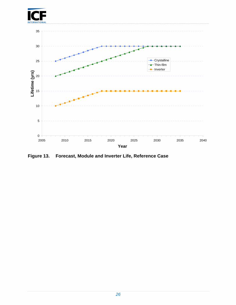
Lifetime. Crystalline PV modules and balance of plant components (except the inverter) are forecast to have an expected lifetime of 25 years in 2008. Thin-film modules and balance of plant components (except the inverter) are forecast to have a lifetime of 20 years in 2008. Both technologies are forecast to have a lifetime of 30 years by 2035. Inverters, which are assumed to be identical for both crystalline and thin-film technologies, are forecast to have lifetime of 10 years in 2008, rising to 15 years by 2035.
Residential Installed Capital Costs (expressed in 2008 dollars). For residential systems, crystalline technologies are forecast to have lower costs compared to thin-film technologies. Forecast costs for installed residential PV systems are approximately $7,100/kWDC (crystalline) and $7,300/kWDC (thin-film) in 2010. These costs fall to approximately $4,000/kWDC (crystalline) and $4,100/kWDC (thin-film) by 2035.
Commercial Installed Capital Costs (expressed in 2008 dollars). For commercial applications, thin-film technologies are forecast to have lower costs compared to crystalline systems (reverse situation compared to residential systems). In 2010, forecast costs for installed commercial PV systems are in the range of $5,500/kWDC (thin-film, 25 kWDC) to $6,800 (crystalline, 25 kWDC). By 2035, forecast costs are estimated to decline to an approximate range of $3,200/kWDC (thin-film, 25 kWDC and 250 kWDC) to $3,800/kWDC (crystalline, 25 kWDC)
O&M Costs. O&M consists of periodic system inspection and solar panel cleaning. For forecasting purposes, it is assumed that both commercial and residential PV system owners will properly maintain their systems. Residential homeowners will likely take a “do it yourself” approach, while commercial sites will use a maintenance contract. In the case of a DIY approach, a cost is still incurred in terms of time required to complete the maintenance. O&M is assumed to scale in direct proportion to panel size, which decreases as module efficiency increases, and with overall system capacity (decreases as capacity increases). Crystalline O&M costs are forecast to decline 30% between 2008 and 2035, reaching levels in the range of $11.20/ kWDC to $$16.80/kWDC by 2035. For thin-film, forecast costs decline 29%, reaching levels in the range of $16.00/kWDC to $24.80/kWDC by 2035.
The recommended characteristics described above correspond to a reference case, or business-as-usual, scenario. In addition to a reference case analysis, an advanced case was developed based on more aggressive assumptions concerning technology advancements and market penetration. The primary difference between the reference case and the advanced case is that installed capital costs decline more quickly over time in the advanced case as a result of accelerated R&D investments.

1
1. Introduction
The Energy Information Administration (EIA) produces a wide range of analyses and reports, including forecasts for energy supply and demand, and the diffusion of technologies in the marketplace. To develop forecasts, EIA uses the National Energy Modeling System (NEMS), which is a robust model that describes energy markets in the United States. Each year, EIA produces the Annual Energy Outlook (AEO), which includes projections generated with NEMS. The AEO report covers a time horizon of 25 to 30 years, and includes market penetration estimates for a wide range of technologies, including residential and commercial photovoltaic (PV) systems.
To develop reliable projections using NEMS, it is important to have accurate technical performance and cost characteristics describing supply side and demand side technologies. Regarding demand side technologies, the residential and commercial PV characteristics that EIA has previously used to support NEMS are based on a solar roadmap baseline projection prepared in 2004.3
1.1 Objective
The objective of this project was to develop a recommended set of technical performance and cost characteristics for residential and commercial PV technologies for the time period extending from 2010 to 2035.
1.2 Approach
ICF conducted a comprehensive literature review and talked with solar experts at manufacturing organizations, national laboratories, and academic institutions. This information was analyzed and used to shape a forecast of PV characteristics through 2035. Recommended characteristics were developed for six PV system prototypes as shown in Table 2. The 5 kWDC size is intended to be representative of residential applications, and the 25 and 250 kWDC capacities are consistent with commercial installations (25 kWDC at the low end, and 250 kWDC at the high end).
Table 2. PV Prototypes
Capacity (kWDC)4 Technology 5, 25, 250 Crystalline 5, 25, 250 Thin-film
As indicated in Table 2, the prototypes are based on crystalline and thin-film solar cell technology. Multi-junction technologies were also evaluated. However, multi-junction technologies are not expected to have significant market penetration in residential and 3 Our Solar Power Future, The U.S. Photovoltaics Industry Roadmap Through 2030 and Beyond, September 2004. 4 Unless noted otherwise, all PV power ratings (kWDC) in this report are based on direct current (DC) at standard test conditions (STC). Standard test conditions are 1,000 W/m2 of solar irradiance, cell temperature of 25 oC, and air mass (AM) of 1.5.
2
commercial applications in the foreseeable future, and prototypes were therefore based only on crystalline and thin-film systems.
Using the prototypes shown in Table 2, a set of recommended PV characteristics was developed that is consistent with a reference case scenario. The reference case scenario is intended to reflect a business-as-usual outcome, assuming that the current pace of R&D investments and policy drivers will prevail over the forecast time horizon. In addition to the reference case scenario, a set of recommended PV characteristics was also developed for an advanced case. The advanced case is based on a scenario that includes higher levels of R&D investments that may accelerate the adoption of residential and commercial PV.
1.3 Report Organization
This report is organized as shown in Table 3. An overview of PV technologies is provided in Section 2, followed by a discussion of markets in Section 3. Historical cost trends from 1998 through 2008 are covered in Section 4. In Section 5, PV characteristics used in the AEO 2010 report are discussed. Results from discussions with PV experts and the literature search are presented in Section 6. In Section 7, recommended PV characteristics for a reference case are presented, and in Section 8 characteristics for an advanced case are described.
Table 3. Report Organization
Section Title 1 Introduction 2 Technologies 3 Markets 4 Historical Costs 5 Forecast of PV Characteristics – Reference Case 6 Forecast of PV Characteristics – Advanced Case
3
2. Technologies
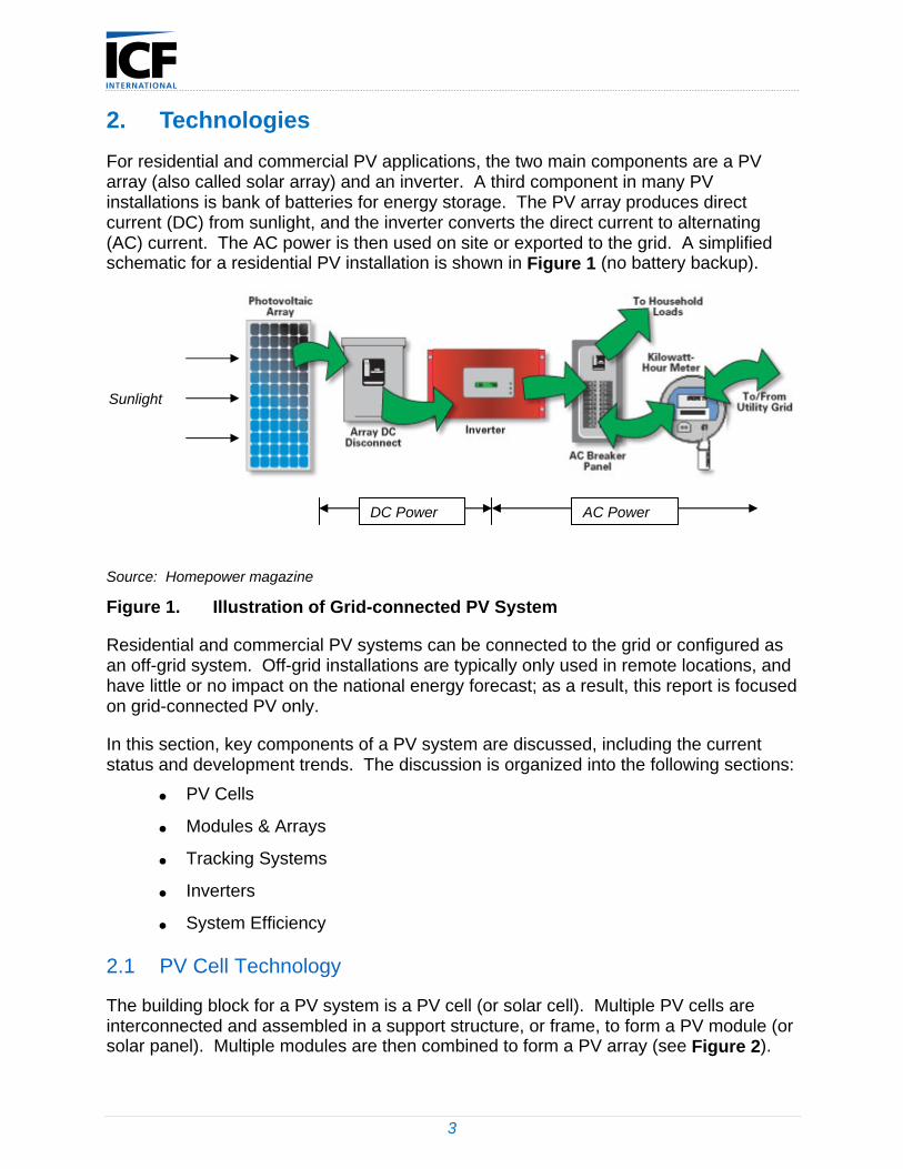
For residential and commercial PV applications, the two main components are a PV array (also called solar array) and an inverter. A third component in many PV installations is bank of batteries for energy storage. The PV array produces direct current (DC) from sunlight, and the inverter converts the direct current to alternating (AC) current. The AC power is then used on site or exported to the grid. A simplified schematic for a residential PV installation is shown in Figure 1 (no battery backup).
Source: Homepower magazine
Figure 1. Illustration of Grid-connected PV System
Residential and commercial PV systems can be connected to the grid or configured as an off-grid system. Off-grid installations are typically only used in remote locations, and have little or no impact on the national energy forecast; as a result, this report is focused on grid-connected PV only.
In this section, key components of a PV system are discussed, including the current status and development trends. The discussion is organized into the following sections:
PV Cells
Modules & Arrays
Tracking Systems
Inverters
System Efficiency
2.1 PV Cell Technology
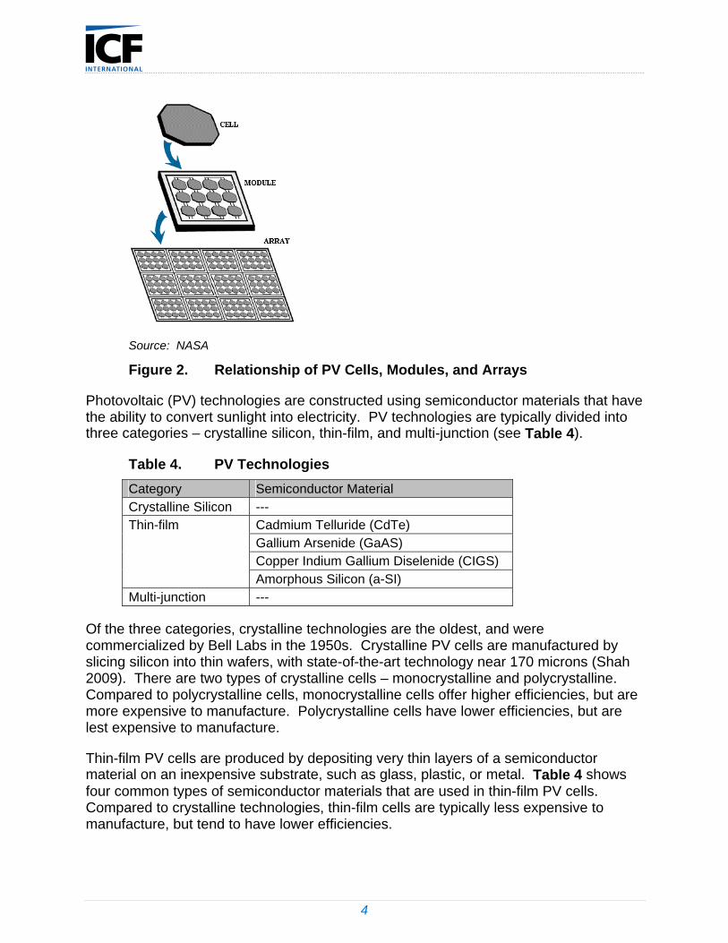
The building block for a PV system is a PV cell (or solar cell). Multiple PV cells are interconnected and assembled in a support structure, or frame, to form a PV module (or solar panel). Multiple modules are then combined to form a PV array (see Figure 2).
DC Power AC Power
Sunlight
4
Source: NASA
Figure 2. Relationship of PV Cells, Modules, and Arrays
Photovoltaic (PV) technologies are constructed using semiconductor materials that have the ability to convert sunlight into electricity. PV technologies are typically divided into three categories – crystalline silicon, thin-film, and multi-junction (see Table 4).
Table 4. PV Technologies
Category Semiconductor Material Crystalline Silicon ---
Cadmium Telluride (CdTe) Gallium Arsenide (GaAS) Copper Indium Gallium Diselenide (CIGS)
Thin-film
Amorphous Silicon (a-SI) Multi-junction ---
Of the three categories, crystalline technologies are the oldest, and were commercialized by Bell Labs in the 1950s. Crystalline PV cells are manufactured by slicing silicon into thin wafers, with state-of-the-art technology near 170 microns (Shah 2009). There are two types of crystalline cells – monocrystalline and polycrystalline. Compared to polycrystalline cells, monocrystalline cells offer higher efficiencies, but are more expensive to manufacture. Polycrystalline cells have lower efficiencies, but are lest expensive to manufacture.
Thin-film PV cells are produced by depositing very thin layers of a semiconductor material on an inexpensive substrate, such as glass, plastic, or metal. Table 4 shows four common types of semiconductor materials that are used in thin-film PV cells. Compared to crystalline technologies, thin-film cells are typically less expensive to manufacture, but tend to have lower efficiencies.

5
Multi-junction cells are fabricated using thin-film techniques, but have two or more different semiconductor materials. The semiconductor materials in a multi-junction cell capture solar energy from different ranges of the solar spectrum, thereby optimizing the conversion of solar energy to electricity. Compared to crystalline and thin-film technologies, multi-junction cells are significantly more expensive to manufacture. Due to the high cost, multi-junction cells do not currently compete in residential and commercial markets.
Crystalline Technology – Trends and Observations
Crystalline modules have dominated residential and commercial PV markets. Crystalline cell efficiencies in the field have improved from approximately 11% to over 14% over the past five years (Shah 2009, Barnett 2009). , Efficiencies in the lab, which are higher than efficiencies in the field, have reached 26% under standard test conditions (STC) (Green 2009).
In recent years, the silicon wafer thickness has been reduced from approximately 300 to 170 microns, and manufacturers have generally increased warranty times from 20 to 25 years. Crystalline cell research is currently focused on reducing material costs, increasing efficiencies, improving the manufacturing processes, and improving reliability of modules (DOE 2008).
Thin-film Technology – Observations and Trends
Over the past five years, thin-film efficiencies have increased from the range of 5-8% to approximately 10% (Barnett 2009). The thin-film market is currently dominated by modules using cadmium telluride (CdTe) as a semiconductor (Maycock and Bradford 2007; Ullal and von Roedern 2007; Venkataraman 2009). In the lab, CdTe modules have reached efficiencies greater than 16% (Green 2009). Two emerging thin-film technologies are copper indium diselenide (CIS) and copper indium gallium diselenide (CIGS). These two cell technologies have shown lab efficiencies of approximately 19% (Green 2009). Another thin-film technology is based on the deposition of amorphous silicon (a-Si) less than a micron thick (Maycock and Bradford 2007). One advantage of a-Si is that these cells can be manufactured in long continuous rolls rather than by batch production (Maycock and Bradford 2007).
Thin-film technologies continue to undergo advancements. CdTe manufacturers are working to standardize film growth equipment, achieve higher efficiencies, and prevent moisture ingress (Ullal 2007). CIGS manufacturers are developing standardized layer deposition equipment and working to achieve higher efficiencies and reduced layer thicknesses (Ullal 2007).
Cell Efficiency – Observations and Trends
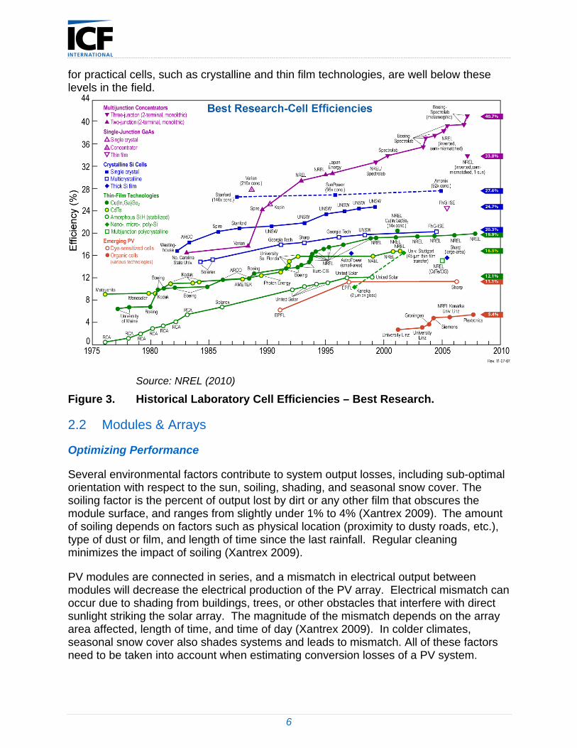
As indicated in Figure 3, solar cell efficiencies have increased at a steady rate over the last several decades (DOE 2006). Efficiencies for advanced multi-junction technologies have approached 40% in laboratory settings at STC conditions. However, efficiencies
6
for practical cells, such as crystalline and thin film technologies, are well below these levels in the field.
Source: NREL (2010)
Figure 3. Historical Laboratory Cell Efficiencies – Best Research.
2.2 Modules & Arrays
Optimizing Performance
Several environmental factors contribute to system output losses, including sub-optimal orientation with respect to the sun, soiling, shading, and seasonal snow cover. The soiling factor is the percent of output lost by dirt or any other film that obscures the module surface, and ranges from slightly under 1% to 4% (Xantrex 2009). The amount of soiling depends on factors such as physical location (proximity to dusty roads, etc.), type of dust or film, and length of time since the last rainfall. Regular cleaning minimizes the impact of soiling (Xantrex 2009).
PV modules are connected in series, and a mismatch in electrical output between modules will decrease the electrical production of the PV array. Electrical mismatch can occur due to shading from buildings, trees, or other obstacles that interfere with direct sunlight striking the solar array. The magnitude of the mismatch depends on the array area affected, length of time, and time of day (Xantrex 2009). In colder climates, seasonal snow cover also shades systems and leads to mismatch. All of these factors need to be taken into account when estimating conversion losses of a PV system.
7
The electrical efficiency of a solar cell in the lab under Standard Test Conditions (STC) is almost always higher than the field efficiency, in part due to temperature differences. For STC measurements, the solar cell is held at 25 oC. The efficiency of a solar cell decreases with increasing temperature, and the field temperature of a solar cell is almost always higher than 25 oC. Roof mounted arrays can reach temperatures of 70-80oC (Wiles 2009). For rooftop conditions, the California Energy Commission recommends a de-rating factor of 89% from STC lab conditions to expected field power (Xantrex 2009).
Building Integrated PV (BIPV)
This report is primarily focused on PV panels that are rack mounted. However, an interesting development is the growth of building integrated PV (BIPV). BIPV technologies are currently more expensive than rack mounted systems, but BIPV breakthroughs could push down PV costs in residential and commercial applications (Chiras 2009).
2.3 Tracking Technology
Maximum PV output occurs when a solar panel is oriented perpendicular to incoming sunlight. The optimum orientation changes through the day as the sun moves across the sky, and on a seasonal basis as the height of the sun above the horizon changes. Tracking systems can be added to PV arrays to optimize electrical output.
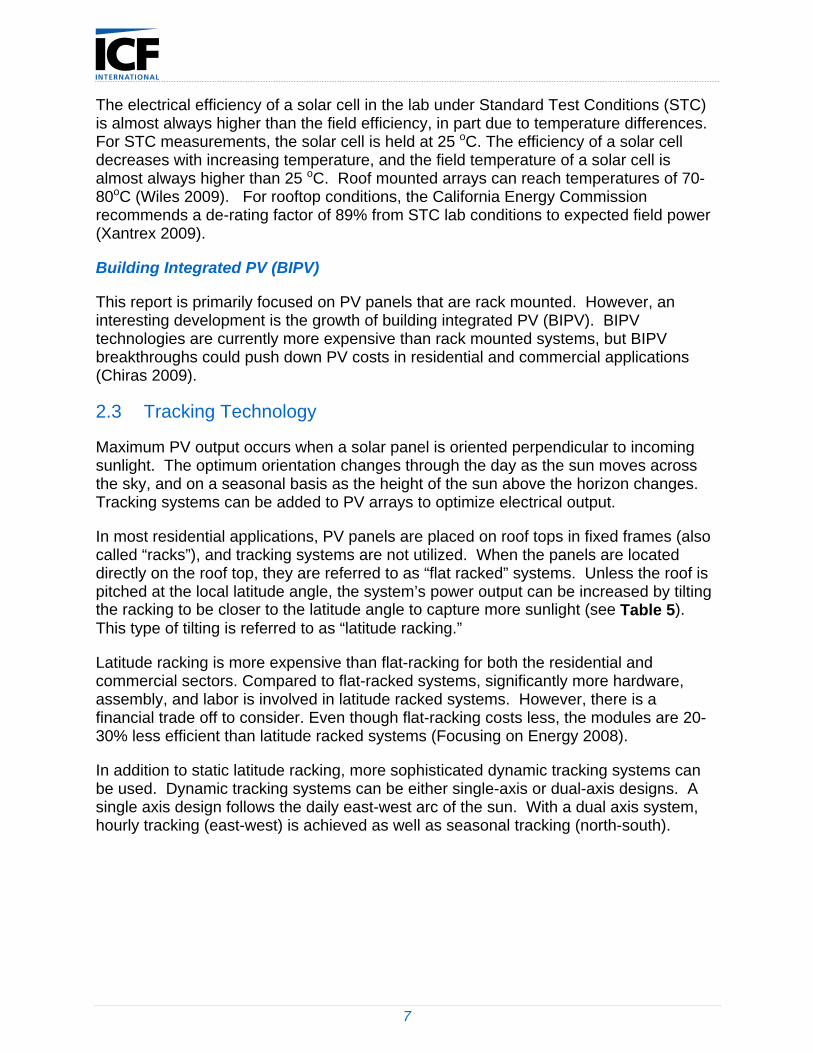
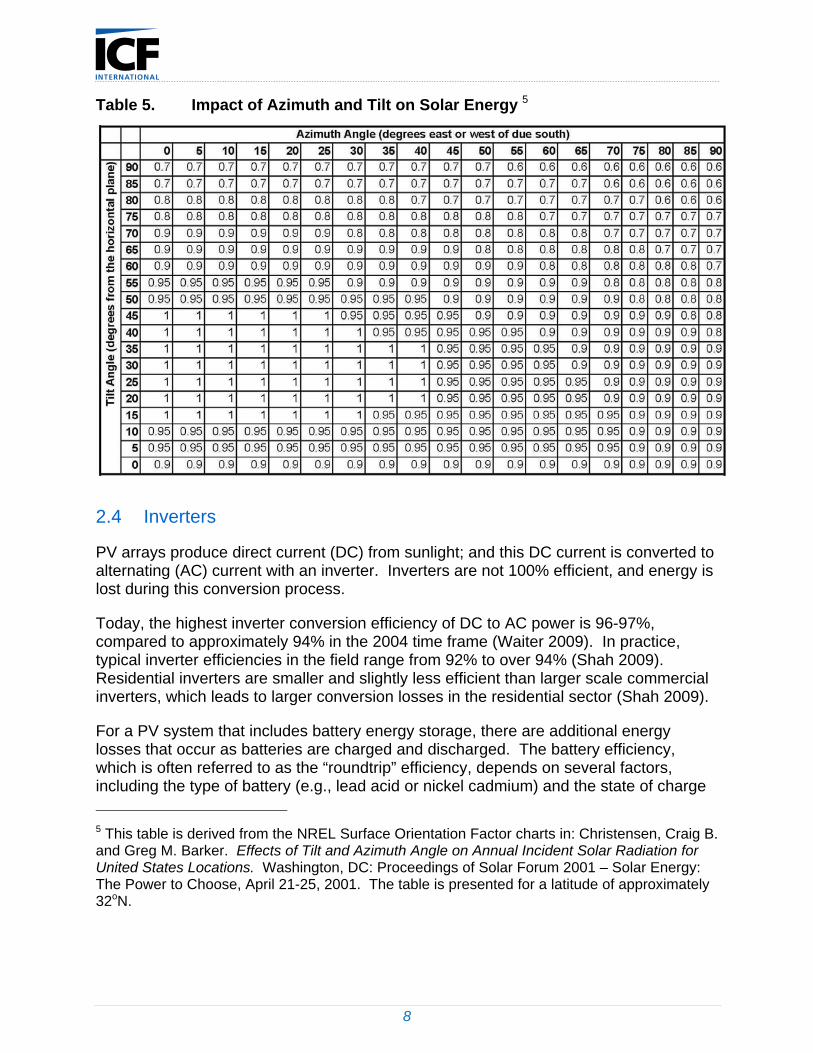
In most residential applications, PV panels are placed on roof tops in fixed frames (also called “racks”), and tracking systems are not utilized. When the panels are located directly on the roof top, they are referred to as “flat racked” systems. Unless the roof is pitched at the local latitude angle, the system’s power output can be increased by tilting the racking to be closer to the latitude angle to capture more sunlight (see Table 5). This type of tilting is referred to as “latitude racking.”
Latitude racking is more expensive than flat-racking for both the residential and commercial sectors. Compared to flat-racked systems, significantly more hardware, assembly, and labor is involved in latitude racked systems. However, there is a financial trade off to consider. Even though flat-racking costs less, the modules are 20-30% less efficient than latitude racked systems (Focusing on Energy 2008).
In addition to static latitude racking, more sophisticated dynamic tracking systems can be used. Dynamic tracking systems can be either single-axis or dual-axis designs. A single axis design follows the daily east-west arc of the sun. With a dual axis system, hourly tracking (east-west) is achieved as well as seasonal tracking (north-south).
8
Table 5. Impact of Azimuth and Tilt on Solar Energy 5
2.4 Inverters
PV arrays produce direct current (DC) from sunlight; and this DC current is converted to alternating (AC) current with an inverter. Inverters are not 100% efficient, and energy is lost during this conversion process.
Today, the highest inverter conversion efficiency of DC to AC power is 96-97%, compared to approximately 94% in the 2004 time frame (Waiter 2009). In practice, typical inverter efficiencies in the field range from 92% to over 94% (Shah 2009). Residential inverters are smaller and slightly less efficient than larger scale commercial inverters, which leads to larger conversion losses in the residential sector (Shah 2009).
For a PV system that includes battery energy storage, there are additional energy losses that occur as batteries are charged and discharged. The battery efficiency, which is often referred to as the “roundtrip” efficiency, depends on several factors, including the type of battery (e.g., lead acid or nickel cadmium) and the state of charge
5 This table is derived from the NREL Surface Orientation Factor charts in: Christensen, Craig B. and Greg M. Barker. Effects of Tilt and Azimuth Angle on Annual Incident Solar Radiation for United States Locations. Washington, DC: Proceedings of Solar Forum 2001 – Solar Energy: The Power to Choose, April 21-25, 2001. The table is presented for a latitude of approximately 32oN.
9
(i.e., near full charge or at some lower charge level). Deep discharge lead acid batteries are frequently used for PV applications, and these batteries have a roundtrip efficiency level typically near 80% (i.e., 80% of the energy used to charge the battery is available for discharge).
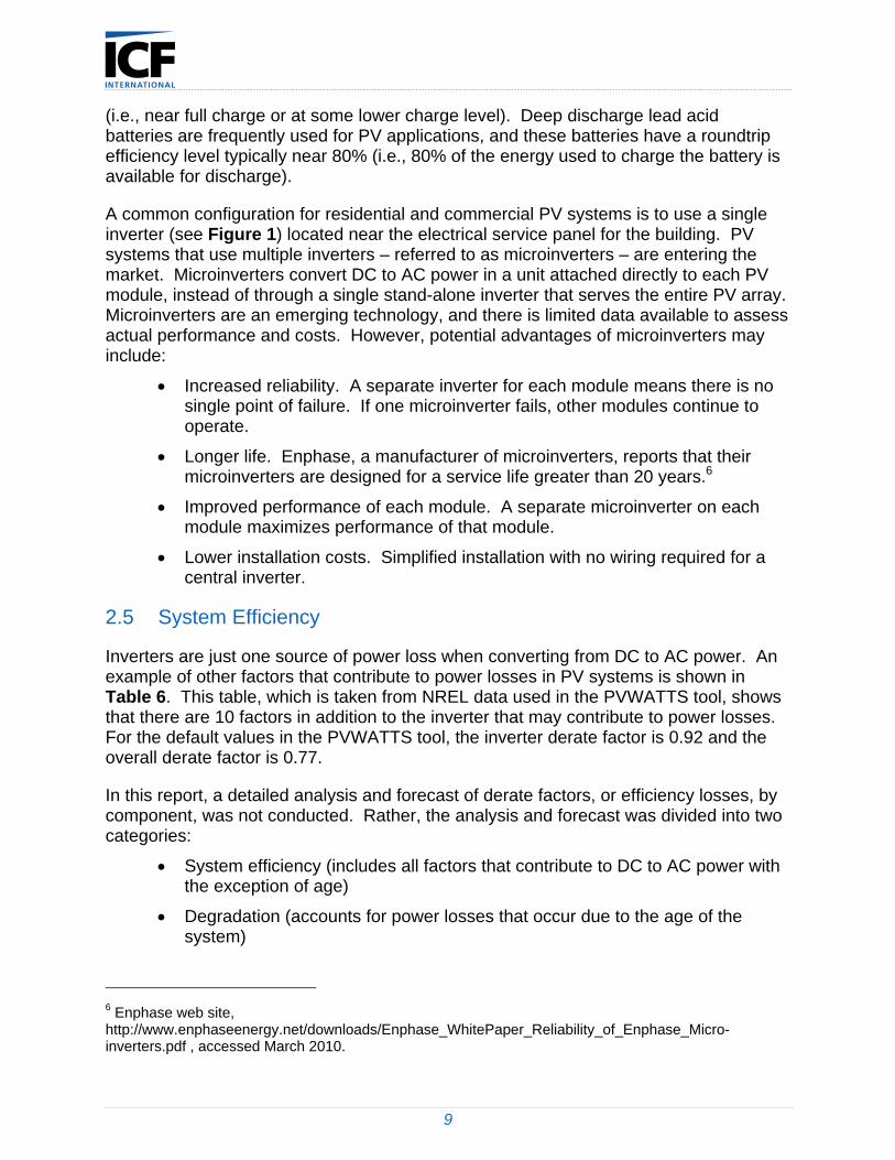
A common configuration for residential and commercial PV systems is to use a single inverter (see Figure 1) located near the electrical service panel for the building. PV systems that use multiple inverters – referred to as microinverters – are entering the market. Microinverters convert DC to AC power in a unit attached directly to each PV module, instead of through a single stand-alone inverter that serves the entire PV array. Microinverters are an emerging technology, and there is limited data available to assess actual performance and costs. However, potential advantages of microinverters may include:
Increased reliability. A separate inverter for each module means there is no single point of failure. If one microinverter fails, other modules continue to operate.
Longer life. Enphase, a manufacturer of microinverters, reports that their microinverters are designed for a service life greater than 20 years.6
Improved performance of each module. A separate microinverter on each module maximizes performance of that module.
Lower installation costs. Simplified installation with no wiring required for a central inverter.
2.5 System Efficiency
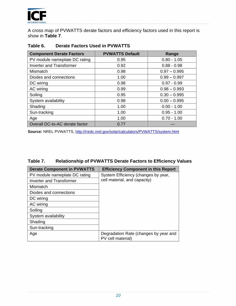
Inverters are just one source of power loss when converting from DC to AC power. An example of other factors that contribute to power losses in PV systems is shown in Table 6. This table, which is taken from NREL data used in the PVWATTS tool, shows that there are 10 factors in addition to the inverter that may contribute to power losses. For the default values in the PVWATTS tool, the inverter derate factor is 0.92 and the overall derate factor is 0.77.
In this report, a detailed analysis and forecast of derate factors, or efficiency losses, by component, was not conducted. Rather, the analysis and forecast was divided into two categories:
System efficiency (includes all factors that contribute to DC to AC power with the exception of age)
Degradation (accounts for power losses that occur due to the age of the system)
6 Enphase web site, http://www.enphaseenergy.net/downloads/Enphase_WhitePaper_Reliability_of_Enphase_Micro-inverters.pdf , accessed March 2010.
10
A cross map of PVWATTS derate factors and efficiency factors used in this report is show in Table 7.
Table 6. Derate Factors Used in PVWATTS
Component Derate Factors PVWATTS Default Range PV module nameplate DC rating 0.95 0.80 - 1.05 Inverter and Transformer 0.92 0.88 - 0.98 Mismatch 0.98 0.97 – 0.995 Diodes and connections 1.00 0.99 – 0.997 DC wiring 0.98 0.97 - 0.99 AC wiring 0.99 0.98 – 0.993 Soiling 0.95 0.30 – 0.995 System availability 0.98 0.00 – 0.995 Shading 1.00 0.00 - 1.00 Sun-tracking 1.00 0.95 - 1.00 Age 1.00 0.70 - 1.00 Overall DC-to-AC derate factor 0.77 ---
Source: NREL PVWATTS, http://rredc.nrel.gov/solar/calculators/PVWATTS/system.html
Table 7. Relationship of PVWATTS Derate Factors to Efficiency Values
Derate Component in PVWATTS Efficiency Component in this Report PV module nameplate DC rating Inverter and Transformer Mismatch Diodes and connections DC wiring AC wiring Soiling System availability Shading Sun-tracking
System Efficiency (changes by year, cell material, and capacity)
Age Degradation Rate (changes by year and PV cell material)

11
3. Markets
3.1 U.S. Market Perspective
Federal, state, and utility incentives provide strong drivers that push the adoption of PV systems. At the Federal level, there is an investment tax credit (ITC), which provides an income tax credit for residential and commercial PV installations. The ITC was revised in 2009 as part of the American Recovery and Reinvestment Act (ARRA). ITC provisions in ARRA that specifically relate to PV include:
30% ITC extended through end of 2016 for both residential and commercial solar installations
$2,000 cap eliminated for residential PV
Utilities allowed to benefit from credit (utilities were previously excluded)
Tax payers (both individuals and businesses) that are required to file Alternative Minimum Tax (AMT) are allowed to claim credit (previously excluded)
PV market size, maturity, and total installed costs vary widely from state to state. The growth of residential and commercial PV markets within a state has been driven almost entirely by state-based incentive programs (Venkataraman 2009). The overwhelming majority of residential and commercial PV installations have occurred in just two states – California and New Jersey (Wiser 2009). Both of these states have well developed incentive programs that have stimulated PV adoption.
In addition to capacity based incentives and performance based incentives, states have used a variety of other tools to encourage the installation of PV, including sales and property tax exemptions, net metering laws, feed-in tariffs, solar access laws, standardized and liberalized interconnection procedures, etc. The incentive mix changes continuously; refer to the Database of State Incentives for Renewables and Efficiency (DSIRE) for the most recent information (DSIRE 2009).
3.2 Installation and Financing
Historically, the installation of PV systems has been performed by companies that specialize in PV. However, the drop in demand for new construction and building retrofit work, coupled with growing demand for end-use PV, has motivated construction companies, roofing contractors, and electrical contractors to enter the PV installation business (Shah 2009). With their project management and business experience, these companies are streamlining the installation process and increasing competition within the industry.
In addition, new financing methods have begun to emerge that are encouraging the adoption of PV systems. The financial factors that influence a consumer’s decision to purchase include upfront costs, financial incentives, utility bill savings, and maintenance costs. Due to the current weak economic conditions, residential homeowners and
12
commercial building owners/developers are reluctant to make expensive capital investments such as PV (Coughlin 2009). New financing methods, such as the commercial solar power purchase agreement (SPPA) and the residential solar lease, seek to overcome these financial barriers by significantly reducing or eliminating the upfront cost to commercial and residential customers (Coughlin 2009).
3.3 International Market Volatility
The U.S. PV industry is influenced by the volatility of the larger international solar market. Manufacturers focus their attention, and their sales, on the fastest growing and most profitable markets. For example, Spain’s feed-in tariff motivated rapid growth and made Spain the largest PV market in the world in 2008. Unprecedented demand in Spain put a strain on global supply that kept equipment costs high in the U.S. and elsewhere in the world (Tarbell 2009). Growth in Spain has slowed recently, but growth in other markets has picked up. For example, Germany installed 3.8 GW of PV in 2009, and 1.45 GW in December alone.7
7 http://www.pv-tech.org/lib/printable/8828, accessed May 2010.
13
4. Historical Costs
Historical costs for PV systems are discussed in this section, which is organized as follows:
Installed PV System Costs
Component Costs
4.1 Installed PV System Costs
Technological developments across the PV supply chain, from commodities to efficiencies, have pushed total installed costs downward. An increase in silicon manufacturing has increased supply and lowered the price of silicon in crystalline PV modules (Hasan 2009). Improved manufacturing processes have increased the production output of facilities, while decreasing the costs of production (GT Solar 2009).
In recent years, streamlined manufacturing has led to decreased manufacturing costs.
Machine manufacturers have begun to offer turn-key production lines which are complete manufacturing system packages. Turn-key solutions are sold for every stage of the supply chain, from wafer fabrication to module fabrication (GT Solar 2009). These automated turn-key production lines have helped increase productivity, quality, and yields, while lowering manufacturing costs. Automated systems have also made it easier for new firms to enter the manufacturing arena, thereby increasing competition and putting downward pressure on prices.
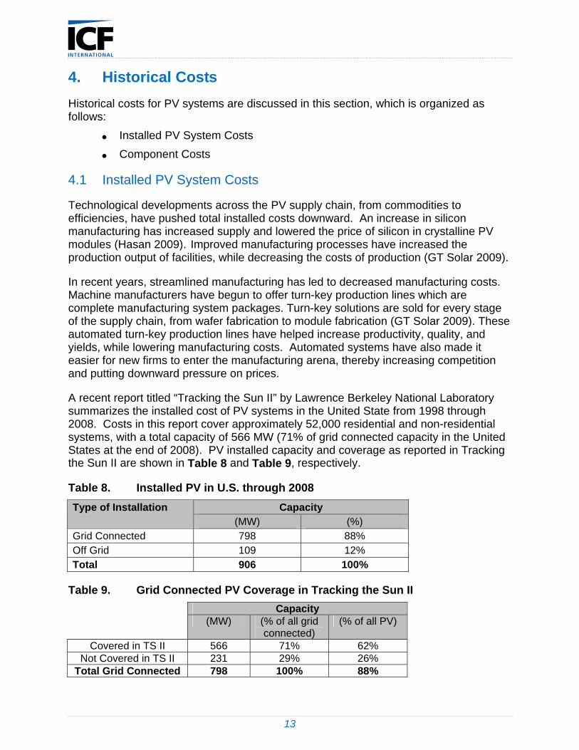
A recent report titled “Tracking the Sun II” by Lawrence Berkeley National Laboratory summarizes the installed cost of PV systems in the United State from 1998 through 2008. Costs in this report cover approximately 52,000 residential and non-residential systems, with a total capacity of 566 MW (71% of grid connected capacity in the United States at the end of 2008). PV installed capacity and coverage as reported in Tracking the Sun II are shown in Table 8 and Table 9, respectively.
Table 8. Installed PV in U.S. through 2008
Capacity Type of Installation (MW) (%)
Grid Connected 798 88% Off Grid 109 12% Total 906 100%
Table 9. Grid Connected PV Coverage in Tracking the Sun II
Capacity (MW) (% of all grid
connected) (% of all PV)
Covered in TS II 566 71% 62% Not Covered in TS II 231 29% 26%
Total Grid Connected 798 100% 88%
14
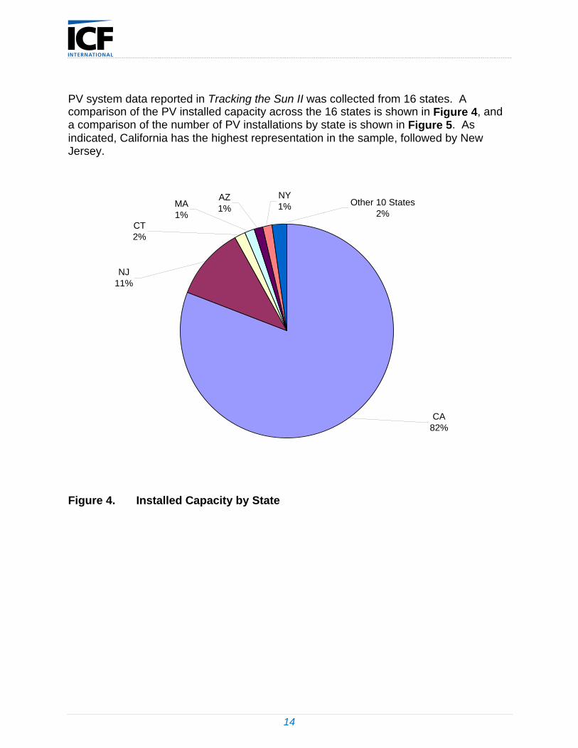
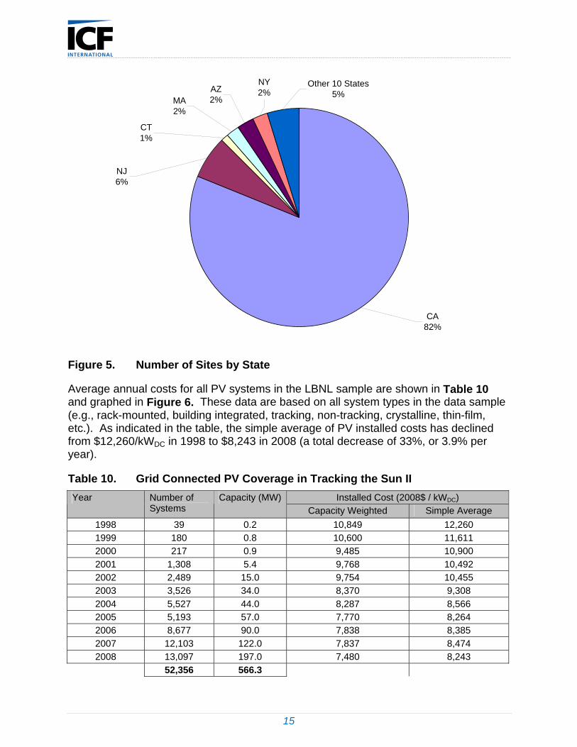
PV system data reported in Tracking the Sun II was collected from 16 states. A comparison of the PV installed capacity across the 16 states is shown in Figure 4, and a comparison of the number of PV installations by state is shown in Figure 5. As indicated, California has the highest representation in the sample, followed by New Jersey.
AZ1%MA
1%CT2%
NY1% Other 10 States
2%
NJ11%
CA82%
Figure 4. Installed Capacity by State
15
NY2%AZ
2%MA2%
CT1%
NJ6%
Other 10 States5%
CA82%
Figure 5. Number of Sites by State
Average annual costs for all PV systems in the LBNL sample are shown in Table 10 and graphed in Figure 6. These data are based on all system types in the data sample (e.g., rack-mounted, building integrated, tracking, non-tracking, crystalline, thin-film, etc.). As indicated in the table, the simple average of PV installed costs has declined from $12,260/kWDC in 1998 to $8,243 in 2008 (a total decrease of 33%, or 3.9% per year).
Table 10. Grid Connected PV Coverage in Tracking the Sun II
Installed Cost (2008$ / kWDC) Year Number of Systems
Capacity (MW)
Capacity Weighted Simple Average
1998 39 0.2 10,849 12,260
1999 180 0.8 10,600 11,611
2000 217 0.9 9,485 10,900
2001 1,308 5.4 9,768 10,492
2002 2,489 15.0 9,754 10,455
2003 3,526 34.0 8,370 9,308
2004 5,527 44.0 8,287 8,566
2005 5,193 57.0 7,770 8,264
2006 8,677 90.0 7,838 8,385
2007 12,103 122.0 7,837 8,474
2008 13,097 197.0 7,480 8,243
52,356 566.3

16
$0
$2,000
$4,000
$6,000
$8,000
$10,000
$12,000
$14,000
1998 1999 2000 2001 2002 2003 2004 2005 2006 2007 2008
Year
Inst
alle
d C
ost
(2
008
$ / k
WD
C)
Capacity Weighted
Simple Average
Figure 6. PV Installed Cost Trends
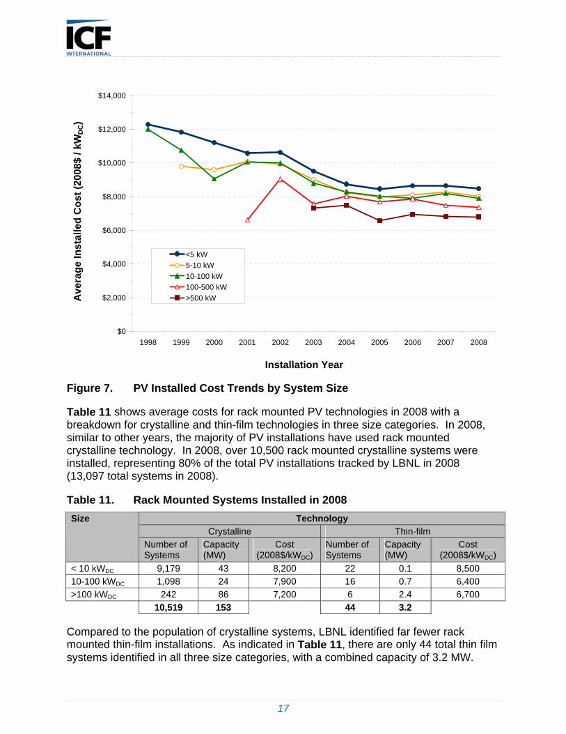
Figure 7 shows a breakout of historical PV costs by size range. Systems less than 100 kWDC showed a steady decline from 1998 through about 2005, and then remained generally flat from 2005 through 2007, followed by a decline in installed costs for 2008. Compared to systems under 100 kWDC, there are far fewer systems with capacities above 100 kWDC, and the data are somewhat more scattered for these larger systems. However, based on Figure 7, it is clear that there are economies of scale, with larger systems consistently showing lower costs.
17
$0
$2,000
$4,000
$6,000
$8,000
$10,000
$12,000
$14,000
1998 1999 2000 2001 2002 2003 2004 2005 2006 2007 2008
Installation Year
Ave
rag
e In
sta
lled
Co
st
(20
08$
/ kW
DC)
<5 kW
5-10 kW
10-100 kW
100-500 kW
>500 kW
Figure 7. PV Installed Cost Trends by System Size
Table 11 shows average costs for rack mounted PV technologies in 2008 with a breakdown for crystalline and thin-film technologies in three size categories. In 2008, similar to other years, the majority of PV installations have used rack mounted crystalline technology. In 2008, over 10,500 rack mounted crystalline systems were installed, representing 80% of the total PV installations tracked by LBNL in 2008 (13,097 total systems in 2008).
Table 11. Rack Mounted Systems Installed in 2008
Technology Crystalline Thin-film
Size
Number of Systems
Capacity (MW)
Cost (2008$/kWDC)
Number of Systems
Capacity (MW)
Cost (2008$/kWDC)
< 10 kWDC 9,179 43 8,200 22 0.1 8,500
10-100 kWDC 1,098 24 7,900 16 0.7 6,400
>100 kWDC 242 86 7,200 6 2.4 6,700
10,519 153 44 3.2
Compared to the population of crystalline systems, LBNL identified far fewer rack mounted thin-film installations. As indicated in Table 11, there are only 44 total thin film systems identified in all three size categories, with a combined capacity of 3.2 MW.
18
While the cost numbers for the thin-film systems seem reasonable (range from $6,400/kWDC to $8,500/kWDC), these results should be viewed with caution given the small sample size. The cost numbers for thin-film technologies could change significantly as the sample size grows and becomes more statistically relevant.
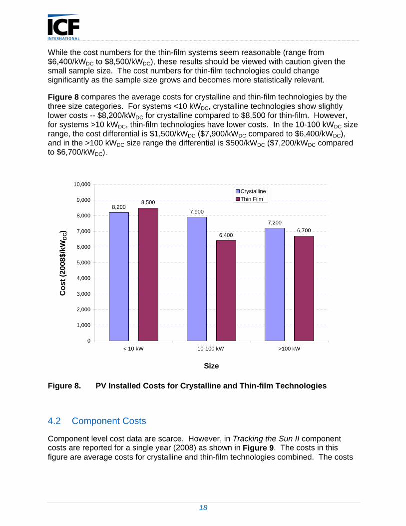
Figure 8 compares the average costs for crystalline and thin-film technologies by the three size categories. For systems <10 kWDC, crystalline technologies show slightly lower costs -- $8,200/kWDC for crystalline compared to $8,500 for thin-film. However, for systems >10 kWDC, thin-film technologies have lower costs. In the 10-100 kWDC size range, the cost differential is $1,500/kWDC ($7,900/kWDC compared to $6,400/kWDC), and in the >100 kWDC size range the differential is $500/kWDC ($7,200/kWDC compared to $6,700/kWDC).
8,2007,900
7,200
8,500
6,4006,700
0
1,000
2,000
3,000
4,000
5,000
6,000
7,000
8,000
9,000
10,000
< 10 kW 10-100 kW >100 kW
Size
Co
st
(20
08$
/kW
DC)
Crystalline
Thin Film
Figure 8. PV Installed Costs for Crystalline and Thin-film Technologies
4.2 Component Costs
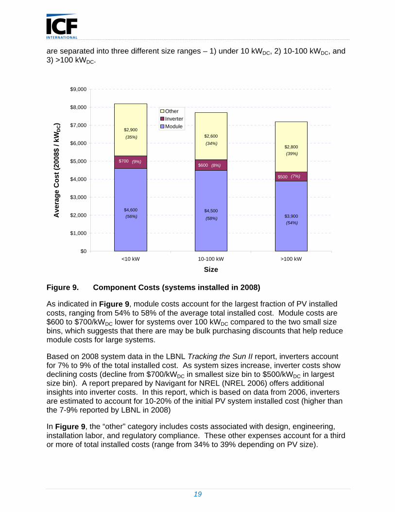
Component level cost data are scarce. However, in Tracking the Sun II component costs are reported for a single year (2008) as shown in Figure 9. The costs in this figure are average costs for crystalline and thin-film technologies combined. The costs
19
are separated into three different size ranges – 1) under 10 kWDC, 2) 10-100 kWDC, and 3) >100 kWDC.
$4,600 $4,500$3,900
$2,900
$2,600
$2,800
$500
$600$700
$0
$1,000
$2,000
$3,000
$4,000
$5,000
$6,000
$7,000
$8,000
$9,000
<10 kW 10-100 kW >100 kW
Size
Av
era
ge
Co
st (
200
8$ /
kW
DC)
Other
Inverter
Module
(56%)
(9%)
(35%)
(58%)
(8%)
(34%)
(54%)
(7%)
(39%)
Figure 9. Component Costs (systems installed in 2008)
As indicated in Figure 9, module costs account for the largest fraction of PV installed costs, ranging from 54% to 58% of the average total installed cost. Module costs are $600 to $700/kWDC lower for systems over 100 kWDC compared to the two small size bins, which suggests that there are may be bulk purchasing discounts that help reduce module costs for large systems.
Based on 2008 system data in the LBNL Tracking the Sun II report, inverters account for 7% to 9% of the total installed cost. As system sizes increase, inverter costs show declining costs (decline from $700/kWDC in smallest size bin to $500/kWDC in largest size bin). A report prepared by Navigant for NREL (NREL 2006) offers additional insights into inverter costs. In this report, which is based on data from 2006, inverters are estimated to account for 10-20% of the initial PV system installed cost (higher than the 7-9% reported by LBNL in 2008)
In Figure 9, the “other” category includes costs associated with design, engineering, installation labor, and regulatory compliance. These other expenses account for a third or more of total installed costs (range from 34% to 39% depending on PV size).
20
5. Forecast of PV Characteristics – Reference Case
While there is ample research and analysis on the size and scope of the PV market, there are few detailed forecasts regarding PV costs and technical performance in the public domain. To develop a PV forecast, ICF collected information from several sources, including interviews with industry PV stakeholders, publicly available literature, and in-house ICF data. The data were grouped into three capacities (5, 25, and 250 kWDC) and two technology types (crystalline and thin-film), resulting in six unique PV technology categories.
No rigid formula was used to develop a composite industry forecast of PV technical performance and cost characteristics. Rather, all data were examined, and data that appeared to lie well outside norms were excluded. The remaining data were further examined and ICF forecasts were developed.
The characteristics described in this section correspond to a reference case scenario consistent with the assumptions used for the reference case described in the AEO 2010 report. The discussion of recommended reference case characteristics is organized as follows:
Technical Performance
o Module Efficiency
o System Efficiency
o Degradation
o Lifetime
Cost
o Component Costs (including inverter)
o Installed Capital
o O&M
For reference, tables with selected results for the reference case are shown in Appendix A (crystalline technologies) and Appendix B (thin-film technologies). In these tables, and elsewhere in this report, costs are reported in 2008 dollars unless noted otherwise. Conversions between dollar years, if necessary, have been calculated using a gross domestic product (GDP) index shown in Appendix C.
5.1 Technical Performance
5.1.1 Module Efficiency
Module efficiencies are primarily dependent on the type of solar cell, and no significant efficiency differences are expected for different capacities. However, different efficiency curves are expected for crystalline and thin-film technologies.

21
To develop a forecast, ICF estimated values for module efficiency when installed in the year 2008, and then looked at potential upper limits. A range of module efficiencies were examined from manufacturers, industry experts, and research reports. Based on this review, ICF selected an average crystalline module efficiency in 2008 of 14%, and an average thin-film module efficiency of 10%. The analysis also suggested that a reasonable upper limit for crystalline modules is 20%, and a reasonable upper limit for thin-film is 14%.
Note that these module efficiencies are based on field performance, and not laboratory measurements. Laboratory measurements conducted at standard test conditions almost always exceed average field performance values.
Linear improvement rates were then developed to connect the starting values and end points. The improvement rates were adjusted by “eye” to achieve a smooth transition over time. The module efficiency forecast parameters are shown in Table 12, and the resulting values are shown in Figure 10.
Table 12. Forecast Parameters, Module Efficiency
PV Cell Technology Crystalline Thin-film
Starting Value (2008) 14% (0.140) 10% (0.100)
Annual Change +0.005 thru 2018 +0.002 thru 2028
+0.001 thru 2028 ---
no change after 2028 no change after 2028
Value in 2035 20% 14%

22
0%
5%
10%
15%
20%
25%
2005 2010 2015 2020 2025 2030 2035
Year
Mo
du
le E
ffic
ien
cy (
%)
Crystalline
Thin-film
Figure 10. Forecast, Module Efficiency, Reference Case
5.1.2 System Efficiency
The overall efficiency of a PV system is determined by several factors, including inverter losses, resistance of wires and connectors, soiling, and module mismatch. While these factors affect all types of PV systems, there are also differences between PV system types. Residential inverters are smaller and therefore less efficient than commercial inverters, leading to generally lower system efficiencies in residential PV technologies (all other factors being equal).
Similar to module efficiencies, linear improvement rates were developed to connect starting values and end points. The improvement rates were adjusted to achieve a smooth transition over time. The system efficiency forecast parameters are shown in Table 13, and the resulting system efficiency curves are shown in Figure 11.

23
Table 13. Forecast Parameters, System Efficiency
PV Cell Technology
Crystalline Thin-film
5 kW 25 kW 250 kW 5 kW 25 kW 250 kW
Starting Value (2008)
78% 80% 82% 77% 79% 81%
+0.01 thru 2012 +0.01 thru 2012
+0.005 thru 2020 +0.005 thru 2022 Annual Change
no change after 2020 no change after 2022
Value in 2035
86% 88% 90% 86% 88% 90%
As indicated, crystalline system efficiencies are expected to increase from levels in the range of 78% to 82% in 2008, to levels in the range of 86% to 90% in 2035. For thin-film technologies, the efficiencies increase from the range of 77% to 81% in 2008, to 86%to 90% by 2035 (same end point for thin film as crystalline).
75%
80%
85%
90%
95%
100%
0 5 10 15 20 25 30
Year
Sys
tem
Eff
icie
ncy
(%
)
Crystalline, 5 kW
Crystalline, 25 kW
Crystalline, 250 kW
Thin-film, 5 kW
Thin-film, 25 kW
Thin-film, 250 kW
Figure 11. Forecast, System Efficiency, Reference Case
24
5.1.3 Degradation
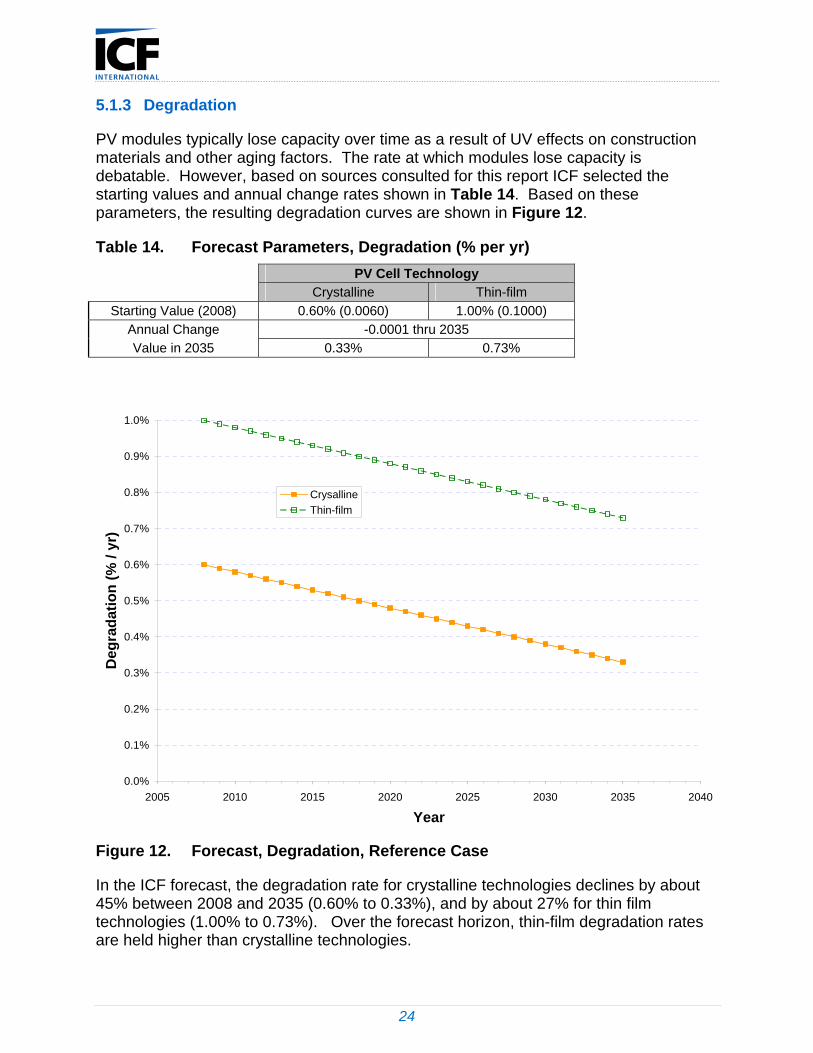
PV modules typically lose capacity over time as a result of UV effects on construction materials and other aging factors. The rate at which modules lose capacity is debatable. However, based on sources consulted for this report ICF selected the starting values and annual change rates shown in Table 14. Based on these parameters, the resulting degradation curves are shown in Figure 12.
Table 14. Forecast Parameters, Degradation (% per yr)
PV Cell Technology Crystalline Thin-film
Starting Value (2008) 0.60% (0.0060) 1.00% (0.1000)
Annual Change -0.0001 thru 2035
Value in 2035 0.33% 0.73%
0.0%
0.1%
0.2%
0.3%
0.4%
0.5%
0.6%
0.7%
0.8%
0.9%
1.0%
2005 2010 2015 2020 2025 2030 2035 2040
Year
Deg
rad
atio
n (
% /
yr)
Crysalline
Thin-film
Figure 12. Forecast, Degradation, Reference Case
In the ICF forecast, the degradation rate for crystalline technologies declines by about 45% between 2008 and 2035 (0.60% to 0.33%), and by about 27% for thin film technologies (1.00% to 0.73%). Over the forecast horizon, thin-film degradation rates are held higher than crystalline technologies.
25
Thin-film technologies have a higher surface area than crystalline systems for equivalent rated capacity, and a higher surface area could contribute to higher degradation rates. However, in general, there are no fundamental reasons that thin-film systems should have higher degradation rates than crystalline systems. However, compared to crystalline technologies, there are fewer thin-film technologies currently being used in residential and commercial applications. The higher degradation rate for thin-film technologies is a conservative value based on a smaller data set with potentially unknown or not-well characterized degradation factors.
5.1.4 Lifetime
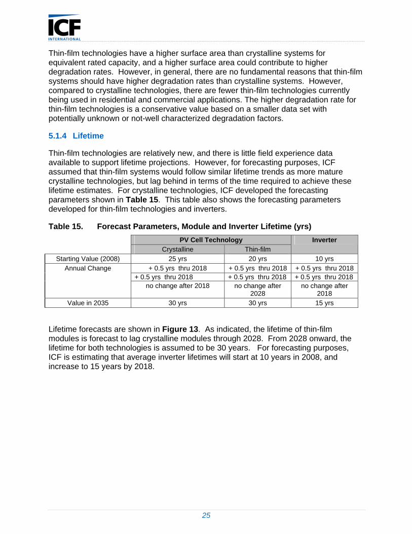
Thin-film technologies are relatively new, and there is little field experience data available to support lifetime projections. However, for forecasting purposes, ICF assumed that thin-film systems would follow similar lifetime trends as more mature crystalline technologies, but lag behind in terms of the time required to achieve these lifetime estimates. For crystalline technologies, ICF developed the forecasting parameters shown in Table 15. This table also shows the forecasting parameters developed for thin-film technologies and inverters.
Table 15. Forecast Parameters, Module and Inverter Lifetime (yrs)
PV Cell Technology Crystalline Thin-film
Inverter
Starting Value (2008) 25 yrs 20 yrs 10 yrs
Annual Change + 0.5 yrs thru 2018 + 0.5 yrs thru 2018 + 0.5 yrs thru 2018 + 0.5 yrs thru 2018 + 0.5 yrs thru 2018 + 0.5 yrs thru 2018 no change after 2018 no change after
2028 no change after
2018
Value in 2035 30 yrs 30 yrs 15 yrs
Lifetime forecasts are shown in Figure 13. As indicated, the lifetime of thin-film modules is forecast to lag crystalline modules through 2028. From 2028 onward, the lifetime for both technologies is assumed to be 30 years. For forecasting purposes, ICF is estimating that average inverter lifetimes will start at 10 years in 2008, and increase to 15 years by 2018.
26
0
5
10
15
20
25
30
35
2005 2010 2015 2020 2025 2030 2035 2040
Year
Lif
etim
e (y
rs)
Crystalline
Thin-film
Inverter
Figure 13. Forecast, Module and Inverter Life, Reference Case

27
5.2 Cost
Long term cost projections for residential and commercial PV installations are scarce in the literature. However, industry stakeholders did provide opinions on long term cost trends. These opinions were combined with ICF in-house data to develop cost projections, which are provided in the following subsections:
Component costs (including inverters)
Installed capital costs
O&M costs
5.2.1 Component Costs
For forecasting purposes, PV components were divided into three categories
Module
Inverter
Other (installation labor, regulatory compliance, and overhead)
ICF set the starting point costs for inverters to be consistent with data reported in the LBNL Tracking the Sun II report (see Figure 9). These inverter starting point costs are shown in Table 16.
Table 16. Starting Point Inverter Costs (2008$/kWDC)
Cost by System Size ($/kWDC) – same for crystalline and thin-film 5 kWDC 25 kWDC 250 kWDC $700 $600 $500
Starting point costs for modules and other components (less the inverter) were combined and calculated by subtracting inverter costs from the total costs reported by LBNL for crystalline and thin-film technologies. These costs are shown in Table 17.
Table 17. Starting Point Costs for Module Plus Other Components (2008$/kWDC)
` Cost by System Size ($/kWDC) 5 kWDC 25 kWDC 250 kWDC
Crystalline $7,500 $7,300 $6,700 Thin-film $7,800 $5,800 $6,200
Cost trends over time were then developed for modules and other components based on input from PV stakeholders and ICF in-house data. Module and other costs (less the inverter) were assumed to follow the same cost trend, which is shown in Figure 14.

28
0%
20%
40%
60%
80%
100%
2008 2010 2012 2014 2016 2018 2020 2022 2024 2026 2028 2030 2032 2034
Year
Co
st R
elat
ive
to 2
008
Figure 14. Normalized Cost Trend for PV Modules and Other Components (does not apply to inverter)
Inverter costs presented somewhat of a dilemma. The technical performance of inverters is evolving (e.g., development of microinverters), but there is mixed information on whether inverter costs are declining or remaining steady. Some PV stakeholders suggested that inverter costs are remaining steady, although price declines have occurred in recent months.8 ICF weighed the limited information available for inverter costs, and chose to forecast inverter costs as remaining unchanged in future years (same costs for crystalline and thin-film technologies). It is expected that inverter performance features will continue to advance, but for forecasting purposes ICF assumed that manufacturers will hold inverter prices relatively constant as inverter performance improves (i.e., inverter value will increase, but prices will remain steady).
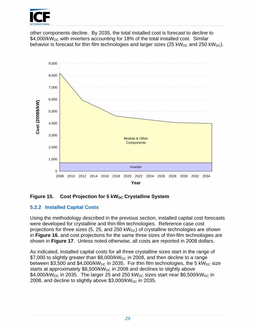
An example of how the forecast costs for modules, inverters, and other components changes over time is shown in Figure 15. This figure corresponds to a 5 kWDC crystalline PV system. As indicated, costs start at $8,200/kWDC ($700 inverter plus $7,500 for module and other components) in 2008, with inverters accounting for 9% of the installed cost. Inverters remain flat over the forecast horizon, while module and
8 Solarbuzz provides an index of monthly inverter and PV module costs (http://www.solarbuzz.com/Inverterprices.htm ).
29
other components decline. By 2035, the total installed cost is forecast to decline to $4,000/kWDC with inverters accounting for 18% of the total installed cost. Similar behavior is forecast for thin film technologies and larger sizes (25 kWDC and 250 kWDC).
Inverter
Module & Other Components
0
1,000
2,000
3,000
4,000
5,000
6,000
7,000
8,000
9,000
2008 2010 2012 2014 2016 2018 2020 2022 2024 2026 2028 2030 2032 2034
Year
Co
st (
200
8$
/kW
)
Figure 15. Cost Projection for 5 kWDC Crystalline System
5.2.2 Installed Capital Costs
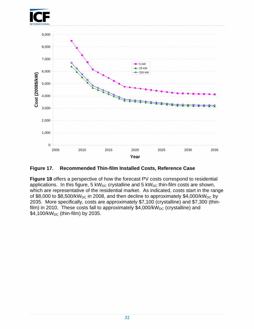
Using the methodology described in the previous section, installed capital cost forecasts were developed for crystalline and thin-film technologies. Reference case cost projections for three sizes (5, 25, and 250 kWDC) of crystalline technologies are shown in Figure 16, and cost projections for the same three sizes of thin-film technologies are shown in Figure 17. Unless noted otherwise, all costs are reported in 2008 dollars.
As indicated, installed capital costs for all three crystalline sizes start in the range of $7,000 to slightly greater than $8,000/kWDC in 2008, and then decline to a range between $3,500 and $4,000/kWDC in 2035. For thin film technologies, the 5 kWDC size starts at approximately $8,500/kWDC in 2008 and declines to slightly above $4,000/kWDC in 2035. The larger 25 and 250 kWDC sizes start near $6,500/kWDC in 2008, and decline to slightly above $3,000/kWDC in 2035.

30
0
1,000
2,000
3,000
4,000
5,000
6,000
7,000
8,000
9,000
2005 2010 2015 2020 2025 2030 2035
Year
Co
st
(200
8$/k
W)
5 kW
25 kW
250 kW
Figure 16. Recommended Crystalline Installed Costs, Reference Case
One unexpected result shown in Figure 17 is that costs for a 250 kWDC thin-film system are forecast to be slightly higher than a 25 kWDC system. Based on economy of scale considerations, one would expect costs for a 250 kWDC system to be lower than a 25 kWDC system. However, these forecasts are consistent with historical costs, which do show an up turn in costs for large thin film PV systems. Historical PV costs are discussed in Section 4.1, and this discussion includes an important note concerning thin-film costs. As mentioned in Section 4.1, historical thin-film costs should be viewed with caution because these costs are based on a small sample size. It would not be surprising if future thin-film costs follow economy of scale considerations (i.e., costs decline as capacities increase).
31
0
1,000
2,000
3,000
4,000
5,000
6,000
7,000
8,000
9,000
2005 2010 2015 2020 2025 2030 2035
Year
Co
st (
200
8$/
kW)
5 kW
25 kW
250 kW
Figure 17. Recommended Thin-film Installed Costs, Reference Case
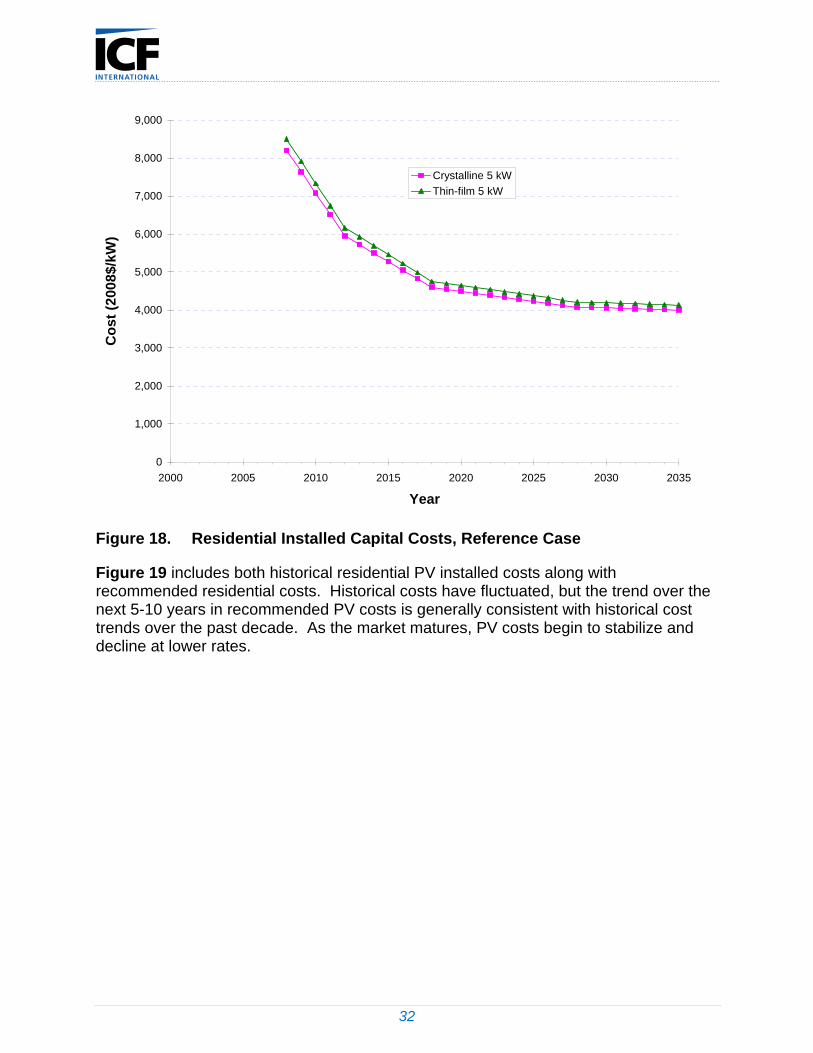
Figure 18 offers a perspective of how the forecast PV costs correspond to residential applications. In this figure, 5 kWDC crystalline and 5 kWDC thin-film costs are shown, which are representative of the residential market. As indicated, costs start in the range of $8,000 to $8,500/kWDC in 2008, and then decline to approximately $4,000/kWDC by 2035. More specifically, costs are approximately $7,100 (crystalline) and $7,300 (thin-film) in 2010. These costs fall to approximately $4,000/kWDC (crystalline) and $4,100/kWDC (thin-film) by 2035.
32
0
1,000
2,000
3,000
4,000
5,000
6,000
7,000
8,000
9,000
2000 2005 2010 2015 2020 2025 2030 2035
Year
Co
st
(200
8$/
kW)
Crystalline 5 kW
Thin-film 5 kW
Figure 18. Residential Installed Capital Costs, Reference Case
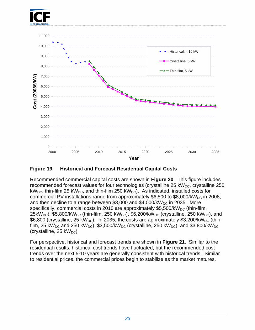
Figure 19 includes both historical residential PV installed costs along with recommended residential costs. Historical costs have fluctuated, but the trend over the next 5-10 years in recommended PV costs is generally consistent with historical cost trends over the past decade. As the market matures, PV costs begin to stabilize and decline at lower rates.
33
0
1,000
2,000
3,000
4,000
5,000
6,000
7,000
8,000
9,000
10,000
11,000
2000 2005 2010 2015 2020 2025 2030 2035
Year
Co
st (
200
8$/
kW)
Historical, < 10 kW
Crystalline, 5 kW
Thin-film, 5 kW
Figure 19. Historical and Forecast Residential Capital Costs
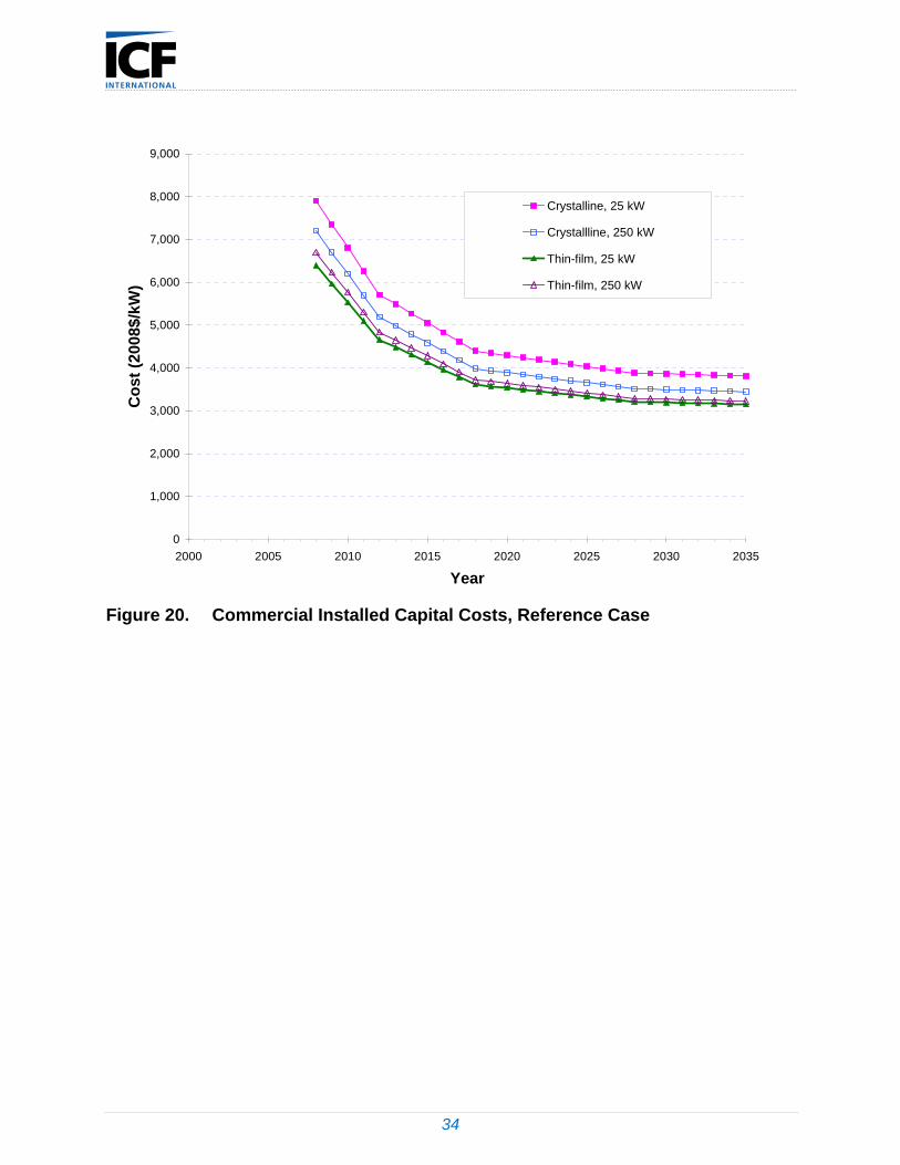
Recommended commercial capital costs are shown in Figure 20. This figure includes recommended forecast values for four technologies (crystalline 25 kWDC, crystalline 250 kWDC, thin-film 25 kWDC, and thin-film 250 kWDC). As indicated, installed costs for commercial PV installations range from approximately $6,500 to $8,000/kWDC in 2008, and then decline to a range between $3,000 and $4,000/kWDC in 2035. More specifically, commercial costs in 2010 are approximately $5,500/kWDC (thin-film, 25kWDC), $5,800/kWDC (thin-film, 250 kWDC), $6,200/kWDC (crystalline, 250 kWDC), and $6,800 (crystalline, 25 kWDC). In 2035, the costs are approximately $3,200/kWDC (thin-film, 25 kWDC and 250 kWDC), $3,500/kWDC (crystalline, 250 kWDC), and $3,800/kWDC (crystalline, 25 kWDC)
For perspective, historical and forecast trends are shown in Figure 21. Similar to the residential results, historical cost trends have fluctuated, but the recommended cost trends over the next 5-10 years are generally consistent with historical trends. Similar to residential prices, the commercial prices begin to stabilize as the market matures.
34
0
1,000
2,000
3,000
4,000
5,000
6,000
7,000
8,000
9,000
2000 2005 2010 2015 2020 2025 2030 2035
Year
Co
st (
2008
$/k
W)
Crystalline, 25 kW
Crystallline, 250 kW
Thin-film, 25 kW
Thin-film, 250 kW
Figure 20. Commercial Installed Capital Costs, Reference Case

35
0
1,000
2,000
3,000
4,000
5,000
6,000
7,000
8,000
9,000
10,000
2000 2005 2010 2015 2020 2025 2030 2035
Year
Co
st
(200
8$/k
W)
Crystalline, 25 kW
Crystalline 250 kW
Thin-film, 25 kW
Thin-film, 250 kW
Historical, >10 kW
Figure 21. Historical and Forecast Commercial Capital Costs
The forecast of installed capital costs presented in this report was developed based on opinions from PV stakeholders and other data sources concerning how costs may change over the next couple decades. The forecast was not developed in conjunction with a detailed demand forecast. While demand was not formerly considered, it is interesting to consider how the installed capital costs projected in this report might be correlated with a demand forecast.
Concerning the relationship of demand and PV costs, a recent EPRI report (EPRI 2009) presented data showing the global average sales price of PV modules as a function of cumulative sales between 1976 and 2008. During this time period, the market size grew by approximately a factor of 100,000 and prices fell by more than 90%. Based on the historical data, the EPRI report authors concluded that prices have been declining by about 20% in recent years for each doubling of market size (i.e., learning rate of 20%). The authors also concluded that the PV market has been growing by about 20% per year in recent years.
The ICF forecast of installed capital costs turns out to be more conservative compared to the results reported by EPRI. In rough terms, the ICF forecast shows a reduction of installed capital costs of approximately 50% between 2008 and 2035. This installed cost behavior is consistent with a learning rate of 12%, and an annual growth rate of
36
15%. The EPRI estimates suggest that learning rates and annual growth rates may both be closer to 20% over the next two to three decades.
5.2.3 O&M
For the purposes of this report, operation and maintenance (O&M) costs are assumed to include regular inspection and cleaning. Major maintenance requirements, such as replacing an inverter, are not included.
For PV systems, routine O&M consists primarily of washing the solar panels to ensure that electricity production is maximized. In both residential and commercial applications, it is possible that systems will not be properly maintained, including periodic washing of PV panels, in which case degradation rates will likely exceed the values reported previously in this report. However, for forecasting purposes, it is assumed that both residential and commercial PV installations will be properly maintained.
In the case of a commercial PV installation, it is reasonable to assume that a maintenance contract will be used to cover O&M. Maintenance contracts for basic service of commercial systems have been reported by SunEdison and others to be in the range of $15/kW to $25/kW (costs generally declining as system size increases).
For a residential PV installation, it is likely that a homeowner will take a “do it yourself” (DIY) approach for system inspection and cleaning. Even though a cash expense is not incurred for a DIY approach, the homeowner does incur an expense in terms of time required to complete PV system O&M. In some residential applications, it is possible that homeowners will choose to pay for routine PV inspection and cleaning, rather than undertaking these chores. In the forecast presented in this report, an O&M cost is assigned to residential PV installations to reflect the value of time for a DIY approach, or the cost of an O&M contract.
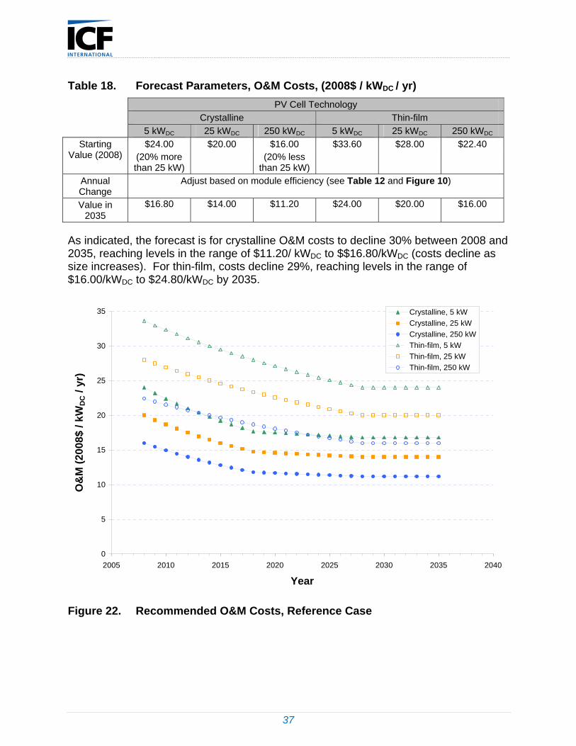
The O&M forecast was developed by starting with a $20/kW O&M cost for a 25 kW crystalline system. Costs were scaled by +/- 20% based on size (5 kW more expensive, 250 kW less expensive). It was further assumed that O&M will scale with surface area, since O&M is primarily associated with panel cleaning. O&M costs were therefore scaled using the module efficiencies discussed previously. A summary of the forecast parameters is shown in Table 18, and a graph of the O&M costs over time is shown in Figure 22.
37
Table 18. Forecast Parameters, O&M Costs, (2008$ / kWDC / yr)
PV Cell Technology
Crystalline Thin-film
5 kWDC 25 kWDC 250 kWDC 5 kWDC 25 kWDC 250 kWDC
$24.00 $20.00 $16.00 $33.60 $28.00 $22.40 Starting Value (2008) (20% more
than 25 kW) (20% less
than 25 kW)
Annual Change
Adjust based on module efficiency (see Table 12 and Figure 10)
Value in 2035
$16.80 $14.00 $11.20 $24.00 $20.00 $16.00
As indicated, the forecast is for crystalline O&M costs to decline 30% between 2008 and 2035, reaching levels in the range of $11.20/ kWDC to $$16.80/kWDC (costs decline as size increases). For thin-film, costs decline 29%, reaching levels in the range of $16.00/kWDC to $24.80/kWDC by 2035.
0
5
10
15
20
25
30
35
2005 2010 2015 2020 2025 2030 2035 2040
Year
O&
M (
2008
$ / k
WD
C /
yr)
Crystalline, 5 kW
Crystalline, 25 kW
Crystalline, 250 kW
Thin-film, 5 kW
Thin-film, 25 kW
Thin-film, 250 kW
Figure 22. Recommended O&M Costs, Reference Case
38
6. Forecast of PV Characteristics – Advanced Case
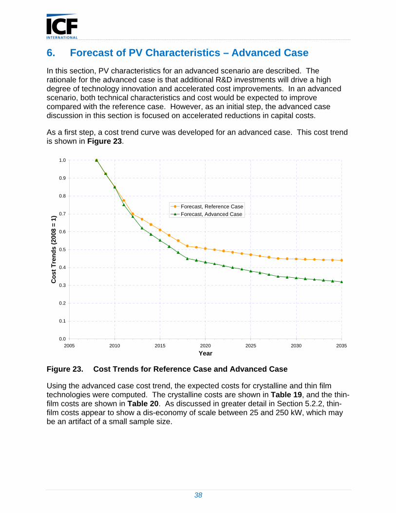
In this section, PV characteristics for an advanced scenario are described. The rationale for the advanced case is that additional R&D investments will drive a high degree of technology innovation and accelerated cost improvements. In an advanced scenario, both technical characteristics and cost would be expected to improve compared with the reference case. However, as an initial step, the advanced case discussion in this section is focused on accelerated reductions in capital costs.
As a first step, a cost trend curve was developed for an advanced case. This cost trend is shown in Figure 23.
0.0
0.1
0.2
0.3
0.4
0.5
0.6
0.7
0.8
0.9
1.0
2005 2010 2015 2020 2025 2030 2035
Year
Co
st
Tre
nd
s (
200
8 =
1)
Forecast, Reference Case
Forecast, Advanced Case
Figure 23. Cost Trends for Reference Case and Advanced Case
Using the advanced case cost trend, the expected costs for crystalline and thin film technologies were computed. The crystalline costs are shown in Table 19, and the thin-film costs are shown in Table 20. As discussed in greater detail in Section 5.2.2, thin-film costs appear to show a dis-economy of scale between 25 and 250 kW, which may be an artifact of a small sample size.

39
Table 19. Crystalline Costs, Reference and Advanced Cases
Cost (2008$ / kWDC)
5 kWDC 25 kWDC 250 kWDC
Year Ref Case Adv
Case Change Ref Case Adv
Case Change Ref Case Adv
Case Change
2010 $7,075 $7,075 0.0% $6,805 $6,805 0.0% $6,195 $6,195 0.0%
2015 $5,275 $4,773 9.5% $5,053 $4,573 9.5% $4,587 $4,151 9.5%
2020 $4,495 $3,820 15.0% $4,294 $3,649 15.0% $3,890 $3,306 15.0%
2025 $4,233 $3,415 19.3% $4,038 $3,258 19.3% $3,656 $2,949 19.3%
2030 $4,054 $3,095 23.6% $3,864 $2,951 23.6% $3,496 $2,669 23.6%
2035 $4,000 $2,909 27.3% $3,812 $2,772 27.3% $3,448 $2,508 27.3%
Table 20. Thin-film Costs, Reference and Advanced Cases
Cost (2008$ / kWDC)
5 kWDC 25 kWDC 250 kWDC
Year Ref Case Adv
Case Change Ref Case Adv
Case Change Ref Case Adv
Case Change
2010 $7,330 $7,330 0.0% $5,530 $5,530 0.0% $5,770 $5,770 0.0%
2015 $5,458 $4,939 9.5% $4,138 $3,745 9.5% $4,282 $3,875 9.5%
2020 $4,647 $3,949 15.0% $3,535 $3,004 15.0% $3,637 $3,091 15.0%
2025 $4,374 $3,529 19.3% $3,332 $2,688 19.3% $3,420 $2,759 19.3%
2030 $4,188 $3,198 23.6% $3,193 $2,438 23.6% $3,272 $2,499 23.6%
2035 $4,132 $3,005 27.3% $3,152 $2,292 27.3% $3,228 $2,348 27.3%
In the advanced scenario, installed capital costs begin diverging from the reference case in 2011, and fall approximately 27% below reference case values by 2035. In the advanced scenario, costs for all components, including the inverter, are reduced at the same rate relative to the reference case.
40
References
Arnoldy, Ben (2008). Brighter future for solar panels: silicon storage eases. The Christian Science Monitor. http://www.csmonitor.com. Accessed October, 2009.
Barnett, A. (December 2009). Personal communication between Lindsay McAlpine, ICF International and Allen Barnett, University of Delaware.
Bartlett, J., Margolis, R., and Jennings, C (September 2009). The Effects of the Financial Crisis on Photovoltaics: An Analysis of Changes in Market Forecasts from 2008-2009. National Renewable Energy Laboratory. http://www.nrel.gov. Accessed October 2009.
Black & Veatch (April 2008). Renewable Energy Transmission Initiative: Phase 1A. RETI Coordinating Committee. http://www.energy.ca.gov. Accessed October 2009.
Blair, N., Mehos, M., and Christensen, C (May 2008). Modeling Photovoltaic and Concentrating Solar Power Trough Performance, Cost and Financing with the Solar Advisor Model. National Renewable Energy Laboratory. http://www.nrel.gov. Accessed November 2009.
Braun, G.W., and Skinner, D.E (January 2007). Experience Scaling-Up Manufacturing of Emerging Photovoltaic Technologies. National Renewable Energy Laboratory. http://www.nrel.gov. Accessed November 2009.
California Solar Initiative (October 2009). California Public Utilities Commission Staff Progress Report. http://www.energy.ca.gov. Accessed November 2009.
Cheyney, Tom (August 2008). Thin-film CIGS starts to come of age. Photovoltaics International. http://www.pv-tech.org. Accessed November 2009.
Chiras, Dan. Power from the Sun: Achieving Energy Independence. New Society Publishers (2009) Canada.
Clean Edge (June 2008). Utility Solar Assessment Study: Reaching Ten Percent Solar by 2025. http://www.greenamericatoday.org. Accessed November 2009.
CleanTechnia (2009). Thin-Film Solar Panels to Double their Share of the Market by 2013? http://cleantechnica.com. Accessed December 2009.
Cory, K., Coughlin, J., and Jenkin, T (February 2008). Innovations in Wind and Solar PV Financing. National Renewable Energy Laboratory. http://www.nrel.gov. Accessed November 2009.
Coughlin, J. and Cory, K. (2009). Solar Photovoltaic Financing: Residential Sector Deployment. National Renewable Energy Laboratory. http://www.nrel.gov. Accessed December 2009.
Curtright, A., Morgan, M., and Keith, D. (2008). Expert Assessments of Future Photovoltaic Technologies. Environmental Science & Technology. http://pubs.acs.org. Accessed November 2009.
41
Denholm, P.; Margolis R.; Ong, S.; Roberts, B. (2009). Break-Even Cost for Residential Photovoltaics in the United States: Key Drivers and Sensitivities. National Renewable Energy Laboratory. http://www.nrel.gov. Accessed December 2009.
Doris, E., McLaren, J., Healey, V., and Hockett, S (October 2009). State of the States 2009: Renewable Energy Development and the Role of Policy. National Renewable Energy Laboratory. http://www.nrel.gov. Accessed November 2009.
Drachman, Philip (October 2009). Third-Generation Thin-Film Solar Technologies: Forecasting the Future of Dye-Sensitized and Organic PV. GTM Research. http://www.researchandmarkets.com. Prometheus Institute/GTM Research. Accessed November 2009.
DSIRE (Database of State Incentives for Renewables and Efficiency). Permitting Incentives. http://www.dsireusa.org. Accessed January 2010.
EPRI (2009). Solar Photovoltaics: Status, Costs, and Trends. December 2009.
Enphase Energy (2009). Microinverter. http://www.enphaseenergy.com. Accessed December 2009.
First Solar (2009). First Solar FS Series 2 PV Module. http://www.firstsolar.com. Accessed January 2010.
Focus on Energy (2008). Selecting a solar electric system for a commercial building rooftop.
Go Solar California (2009-a). List of Eligible Inverters. http://www.gosolarcalifornia.org. Accessed January 2010.
Go Solar California (2009-b). List of Eligible SB1 Guidelines Compliant Photovoltaic Modules. http://www.gosolarcalifornia.org. Accessed January 2010.
Green, M., et al. (2009). Solar Cell Efficiency Tables (Version 33). Progress in Photovoltaics: Research and Applications. http://www3.interscience.wiley.com. 17:85-94. Accessed November 2009.
Gregg, A., Parker, T., and Swenson, R (2005). A “Real World” Examination of PV System Design and Performance. http://ieeexplore.ieee.org. Accessed December 2009.
Grover, S (August 2007). Energy, Economic, and Environmental Benefits of the Solar America Initiative. National Renewable Energy Laboratory. http://www.nrel.gov. Accessed November 2009.
GT Solar (2009). Turnkey Manufacturing Solutions. http://www.gtsolar.com. Accessed December 2009.
Hasan, Russell (2009). The Solar Silicon Shortage and Its Impact on Solar Power Stocks. SolarHome. http://www.solarhome.org. Accessed November 2009.
Homepower (2007). Ask the Experts: PV Longevity & Degradation. http://homepower.com. Accessed January 2010.
42
Kann, Shayle (2009). The United States PV Market through 2013: Project Economics, Policy, Demand, and Strategy. GMT Research. http://www.gtmresearch.com. Accessed December 2009.
KEMA (August 2009). Renewable Energy Cost of Generation Update. California Energy Commission. http://www.energy.ca.gov. Accessed December 2009.
Kerr, M., Campbell, P., and Cuevas, A (2002). Lifetime and Efficiency Limits of Crystalline Silicon Solar Cells. IEEE. http://ieeexplore.ieee.org. Accessed November 2009.
Lewis, N. (2007). Toward Cost-Effective Solar Energy Use. Science. http://www.sciencemag.org. Accessed January 2010.
Maycock, P. and Bradford, T (2007). PV Technology, Performance, and Cost. Prometheus Institute. http://www.prometheus.org. Accessed December 2009.
McConnell, R. and Matson, R (January 2005). Exploratory Research for New Solar Electric Technologies. Nation Renewable Energy Laboratory. http://www.nrel.gov. Accessed November 2009.
Mehta, S. and Bradford, T (January 2009). PV Technology, Production, and Cost, 2009 Forecast: The Anatomy of a Shakeout. Prometheus Institute & GTM Research. http://www.gtmresearch.com. Accessed December 2010.
Mehta, Shyam (September 2009). PV Manufacturing in the United States: Market Outlook, Incentives, and Supply Chain Opportunities. Prometheus Institute & GTM Research. http://www.gtmresearch.com. Accessed November 2009.
NASA, How Do Photovoltaics Work?. http://science.nasa.gov. Accessed May 2010.
National Renewable Energy Laboratory (2010). Best Research – Cell Efficiencies, downloaded from Wikipedia, http://en.wikipedia.org. Accessed March 2010.
National Renewable Energy Laboratory (2009-a). Photovoltaic Research: Electronic Materials and Devices. http://www.nrel.gov. Accessed December 2009.
National Renewable Energy Laboratory (2009-b). Photovoltaic Research: Research and Development. http://www.nrel.gov . Accessed December 2009.
National Renewable Energy Laboratory (2006). A Review of PV Inverter Technology Cost and Performance Projections, Prepared by Navigant Consulting, NREL/SR-620-38771, http://www.nrel.gov, p37, Accessed March 2010.
Navigant (2008). Economic Impacts of Extending Federal Solar Tax Credits. http://www.seia.org. Accessed November 2009.
Osterwald, C.R. and McMahon, T.J (2009). History of Accelerated and Qualification Testing of Terrestrial Photovoltaic Modules: A Literature Review. Progress in Photovoltaics: Research and Applications. http://www.nrel.gov. Accessed January 2010.
43
Paidipati, J., Frantzis, L., Sawyer, H., and Kurrasch, A (February 2008). Rooftop Photovoltaics Market Penetration Scenarios. NREL. http://www.nrel.gov. Accessed December 2009.
Public Renewables Partnership (2010). http://www.repartners.org. Accessed January 2010.
Sandia National Laboratories (2009). Photovoltaic Systems Research & Development. http://photovoltaics.sandia.gov. Accessed January 2010.
Shah, J. (December 2009). Personal communication between Lindsay McAlpine, ICF International and Jigar Shah, Carbon War Room.
Sherwood, Larry (July 2009). U.S. Solar Market Trends 2008. Interstate Renewable Energy Council. http://www.irecusa.org. Accessed November 2009.
Sierra Club (2008). Solar Electric Permit Fees in Northern California: A Comparative Study. http://www.lomaprieta.sierraclub.org/. Accessed January 2010.
Solar Electric Power Association (2009-a). Photovoltaic Markets and Technologies. California Energy Commission. Accessed November 2009.
Solar Energy Industries Association (2009-b). Membership Directory. http://www.seia.org. Accessed November 2009.
Solar Energy Industries Association (2008-a). Federal Issues: The Investment Tax Credit (ITC). http://www.seia.org. Accessed 1/10/10.
Solar Energy Industries Association (2008-b). US Solar Industry Year in Review 2008. http://www.seia.org. Accessed November 2009.
Solarbuzz (2009). Solar Cell Manufacturing Plants. http://www.solarbuzz.com. Accessed November 2009.
Solarbuzz (2010). Solar Module Price Highlights: January 2010. http://www.solarbuzz.com. Accessed January 2010.
SolarHub (2009). PV Modules. http://www.solarhub.com Accessed December 2009.
SPEI (2007). Sizing of grid-connected photovoltaic systems. http://spie.org. Accessed November 2009.
States Advancing Solar (2009). Federal Policies. http://www.statesadvancingsolar.org. Accessed January 2010.
Symko-Davies, Martha (2009). Progress in High-Performance PV: Polycrystalline Thin-Film Tandem Cells. National Renewable Energy Laboratory. http://www.nrel.gov. Accessed November 2009.
U.S. Department of Energy – Energy Efficiency and Renewable Energy (July 2009). Photovoltaics. http://www1.eere.energy.gov. Accessed October 2009.

44
U.S. Department of Energy – Energy Efficiency and Renewable Energy (April 2008). Solar Energy Technologies Program: Multi-Year Program Plan 2008-2012. http://www1.eere.energy.gov. Accessed November 2009.
U.S. Department of Energy – Energy Efficiency and Renewable Energy (January 2008). The Value and Cost of Solar Electricity. http://www1.eere.energy.gov. Accessed November 2009.
U.S. Department of Energy – Energy Efficiency and Renewable Energy (2006-a). Solar Energy Technologies Program: Multi-Year Program Plan 2007-2011. http://www1.eere.energy.gov. Accessed November 2009.
U.S. Department of Energy – Energy Efficiency and Renewable Energy (2006-b). Technologies: Balance of Systems. http://www1.eere.energy.gov. Accessed January 2010.
U.S. Department of Energy – Energy Efficiency and Renewable Energy (September 2004). Our Solar Power Future: The U.S. Photovoltaics Industry Roadmap through 2030 and Beyond. http://www.nrel.gov. Accessed December 2009.
Ullal, H. S (August 2004). Polycrystalline Thin-Film Photovoltaic Technologies: Progress and Technical Issues. National Renewable Energy Laboratory. http://www.nrel.gov. Accessed November 2009.
Ullal, H. S., and von Roedern, B (September 2007). Thin Film CIGS and CdTe Photovoltaic Technologies: Commercialization, Critical Issues, and Applications. NREL. http://www.i-micronews.com. Accessed November 2009.
Venkataraman, S. (2009) Tracking the Economics Of Wholesale And Retail Solar Photovoltaic Generation. www.ratingsdirect.com. Accessed November 2009.
Venkataraman, S. (2009) A Power Surge for the Global Solar Energy. www.ratingsdirect.com. Accessed November 2009.
Venkataraman, S. (2009) Key Credit Factors: Methodology and Assumptions on Risks for Utility-Scale Solar Photovoltaic Projects. www.ratingsdirect.com. Accessed November 2009.
Waiter, S. (December 2009). Personal communication between Lindsay McAlpine, ICF International and Scott Waiter, Standard Solar.
Wang, Ucilia (October 2009). Germany Installs 2.34GW, FIT to Decline 9-11%. Greentechsolar. http://www.greentechmedia.com. Accessed January 2010.
Wiles, John (2009). Roof-Mounted PV System Design Challenges. http://homepower.com. Accessed February 2010.
Wiser, R., Barbose, G., Peterman, C., and Darghouth, N. (2009). Tracking the Sun II: The Installed Cost of Photovoltaics in the U.S. from 1998-2008. http://eetd.lbl.gov. Accessed October 2009.
Wiser, R. and Barbose, G (August 2008). Renewables Portfolio Standards in the United States. Lawrence Berkeley National Laboratory. http://eetd.lbl.gov. Accessed November 2009.
45
Wiser, R., Mills, A., Barbose, G., and Golove, W (July 2007). The Impact of Retail Rate Structures on the Economics of Commercial Photovoltaic Systems in California. Lawrence Berkeley National Laboratory. http://eetd.lbl.gov. Access November 2009.
Wohlgemuth, J (May 2009). Development of Large High-Voltage PV Modules with Improved Reliability and Lower Cost. National Renewable Energy Laboratory. http://www1.eere.energy.gov. Accessed November 2009.
Wohlmuth, Walter (2009). Thin Film CdTe Module Manufacturing. http://www.csmantech.org. Accessed November 2009.
Xantrex. Calculating Actual PV System Output. http://www.xantrex.com. Accessed December 2009.
Zhang, Y. and Smith, J.S (August 2008). Long-Term Modeling of Solar Energy: Analysis of Concentrating Solar Power and PV Technologies. U.S. Department of Energy—Pacific Northwest National Laboratory. http://www.pnl.gov. Accessed November 2009.
Zweibel, K., Mason, J., and Fthenakis, V (December 2007). A Solar Grand Plan. Scientific American. http://www.scientificamerican.com. Accessed January 2010.
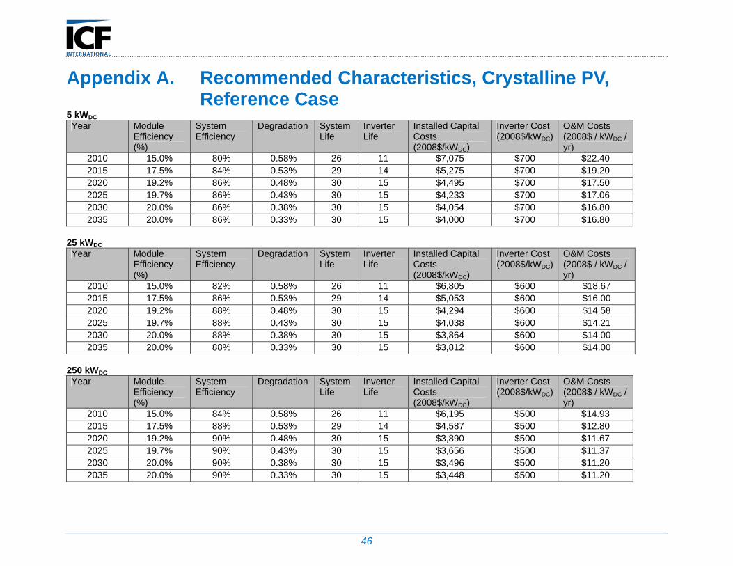
46
Appendix A. Recommended Characteristics, Crystalline PV, Reference Case
5 kWDC Year Module
Efficiency (%)
System Efficiency
Degradation System Life
Inverter Life
Installed Capital Costs (2008$/kWDC)
Inverter Cost (2008$/kWDC)
O&M Costs (2008$ / kWDC / yr)
2010 15.0% 80% 0.58% 26 11 $7,075 $700 $22.40 2015 17.5% 84% 0.53% 29 14 $5,275 $700 $19.20 2020 19.2% 86% 0.48% 30 15 $4,495 $700 $17.50 2025 19.7% 86% 0.43% 30 15 $4,233 $700 $17.06 2030 20.0% 86% 0.38% 30 15 $4,054 $700 $16.80 2035 20.0% 86% 0.33% 30 15 $4,000 $700 $16.80
25 kWDC Year Module
Efficiency (%)
System Efficiency
Degradation System Life
Inverter Life
Installed Capital Costs (2008$/kWDC)
Inverter Cost (2008$/kWDC)
O&M Costs (2008$ / kWDC / yr)
2010 15.0% 82% 0.58% 26 11 $6,805 $600 $18.67 2015 17.5% 86% 0.53% 29 14 $5,053 $600 $16.00 2020 19.2% 88% 0.48% 30 15 $4,294 $600 $14.58 2025 19.7% 88% 0.43% 30 15 $4,038 $600 $14.21 2030 20.0% 88% 0.38% 30 15 $3,864 $600 $14.00 2035 20.0% 88% 0.33% 30 15 $3,812 $600 $14.00
250 kWDC Year Module
Efficiency (%)
System Efficiency
Degradation System Life
Inverter Life
Installed Capital Costs (2008$/kWDC)
Inverter Cost (2008$/kWDC)
O&M Costs (2008$ / kWDC / yr)
2010 15.0% 84% 0.58% 26 11 $6,195 $500 $14.93 2015 17.5% 88% 0.53% 29 14 $4,587 $500 $12.80 2020 19.2% 90% 0.48% 30 15 $3,890 $500 $11.67 2025 19.7% 90% 0.43% 30 15 $3,656 $500 $11.37 2030 20.0% 90% 0.38% 30 15 $3,496 $500 $11.20 2035 20.0% 90% 0.33% 30 15 $3,448 $500 $11.20
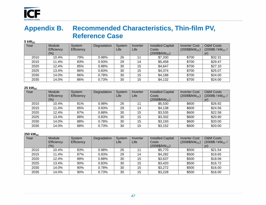
47
Appendix B. Recommended Characteristics, Thin-film PV, Reference Case
5 kWDC Year Module
Efficiency (%)
System Efficiency
Degradation System Life
Inverter Life
Installed Capital Costs (2008$/kWDC)
Inverter Cost (2008$/kWDC)
O&M Costs (2008$ / kWDC / yr)
2010 10.4% 79% 0.98% 26 11 $7,330 $700 $32.31 2015 11.4% 83% 0.93% 29 14 $5,458 $700 $29.47 2020 12.4% 85% 0.88% 30 15 $4,647 $700 $27.10 2025 13.4% 86% 0.83% 30 15 $4,374 $700 $25.07 2030 14.0% 86% 0.78% 30 15 $4,188 $700 $24.00 2035 14.0% 86% 0.73% 30 15 $4,132 $700 $24.00
25 kWDC Year Module
Efficiency (%)
System Efficiency
Degradation System Life
Inverter Life
Installed Capital Costs (2008$/kWDC)
Inverter Cost (2008$/kWDC)
O&M Costs (2008$ / kWDC / yr)
2010 10.4% 81% 0.98% 26 11 $5,530 $600 $26.92 2015 11.4% 85% 0.93% 29 14 $4,138 $600 $24.56 2020 12.4% 87% 0.88% 30 15 $3,535 $600 $22.58 2025 13.4% 88% 0.83% 30 15 $3,332 $600 $20.90 2030 14.0% 88% 0.78% 30 15 $3,193 $600 $20.00 2035 14.0% 88% 0.73% 30 15 $3,152 $600 $20.00
250 kWDC Year Module
Efficiency (%)
System Efficiency
Degradation System Life
Inverter Life
Installed Capital Costs (2008$/kWDC)
Inverter Cost (2008$/kWDC)
O&M Costs (2008$ / kWDC / yr)
2010 10.4% 83% 0.98% 26 11 $5,770 $500 $21.54 2015 11.4% 87% 0.93% 29 14 $4,282 $500 $19.65 2020 12.4% 89% 0.88% 30 15 $3,637 $500 $18.06 2025 13.4% 90% 0.83% 30 15 $3,420 $500 $16.72 2030 14.0% 90% 0.78% 30 15 $3,272 $500 $16.00 2035 14.0% 90% 0.73% 30 15 $3,228 $500 $16.00
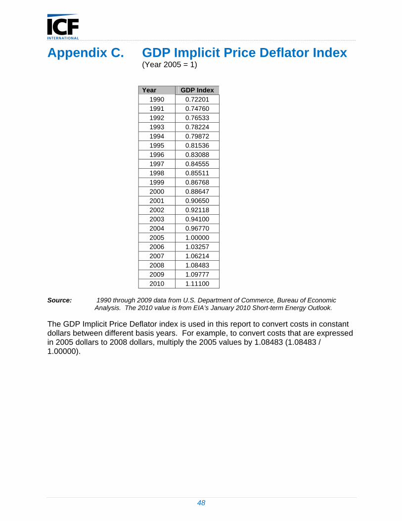
48
Appendix C. GDP Implicit Price Deflator Index (Year 2005 = 1)
Year GDP Index
1990 0.72201
1991 0.74760
1992 0.76533
1993 0.78224
1994 0.79872
1995 0.81536
1996 0.83088
1997 0.84555
1998 0.85511
1999 0.86768
2000 0.88647
2001 0.90650
2002 0.92118
2003 0.94100
2004 0.96770
2005 1.00000
2006 1.03257
2007 1.06214
2008 1.08483
2009 1.09777
2010 1.11100
Source: 1990 through 2009 data from U.S. Department of Commerce, Bureau of Economic Analysis. The 2010 value is from EIA’s January 2010 Short-term Energy Outlook.
The GDP Implicit Price Deflator index is used in this report to convert costs in constant dollars between different basis years. For example, to convert costs that are expressed in 2005 dollars to 2008 dollars, multiply the 2005 values by 1.08483 (1.08483 / 1.00000).

Headquarters
ICF International
9300 Lee Highway
Fairfax, Virginia 22031
www.icfi.com
June 2013
U.S. Energy Information Administration | Distributed Generation System Characteristics and Costs in the Buildings Sector
APPENDIX B
EIA Task Order No. DE-DT0000804, Subtask 3
The Cost and Performance of Distributed Wind Turbines, 2010-35 Final Report June 2010 Prepared for: Office of Integrated Analysis & Forecasting U.S. Energy Information Administration
Prepared by: ICF International
Contact: Robert Kwartin T: (703) 934-3586 E: [email protected]
ii
Table of Contents
Executive Summary ..................................................................................................................... iv Introduction ................................................................................................................................... v 1. Technology Overview............................................................................................................1 2. Market Overview ...................................................................................................................2 3. Potential Market Size ............................................................................................................4
3.1 Technical Factors.......................................................................................................4 3.2 Economic Factors - Benefits ......................................................................................6 3.3 Economic Factors - Costs..........................................................................................7 3.4 Market Potential - Conclusions ..................................................................................7
4. Performance Objectives........................................................................................................8 5. Interpreting Performance Data for Distributed Wind Technology........................................10 6. Data Issues – Implications for NEMS..................................................................................12 7. Technology Baseline...........................................................................................................13 8. Sources for Improvement....................................................................................................14
8.1 Technological...........................................................................................................14 8.2 Cost..........................................................................................................................15
9. Projection Methodology.......................................................................................................17 Endnotes.....................................................................................................................................19 Bibliography ................................................................................................................................21
iii
Tables
Table 1: The U.S. Distributed Wind Market ..................................................................................3 Table 2: Market Projections of Grid-Connected Domestically Installed Wind Turbines ................8 Table 3: Percentage Difference between Manufacturer Literature and NREL Test Data ...........12 Table 4: Dimensional Data for Selected Distributed Wind Turbines ...........................................13 Table 5: Cost and Performance Data for Selected Distributed Wind Turbines, 2009.................14 Table 6: Improvement in the GE 1.5 MW Turbine ......................................................................14 Table 7: Annual Operation and Maintenance Expenses.............................................................16 Table 8: Assumptions for the Base and Advanced Cases..........................................................18
Figures
Figure 1: Main Components of a Wind Turbine ............................................................................1 Figure 2: Growth of the Small Wind Market in the U.S. ................................................................4 Figure 3: National Wind Resource Map ........................................................................................5
Cover photos courtesy of the American Wind Energy Association.
iv
Executive Summary
This report and its accompanying data tables provide cost and performance projections for distributed wind turbines in the 1-100 kW nominal size range over the 2010-35 period. These factors were developed by compiling manufacturer-provided cost and performance of popular present-day turbines in this size range; adjusting these 2009 data to reflect independent test results and to conform to new data definitions that will apply in 2010 and beyond; and then developing cost and performance trajectories for the forecast period. These trajectories are based on interviews with market participants, particularly manufacturers, distributed wind project developers, and researchers.
Projections were developed for both a reference case and an advanced case. The advanced case is distinguished from the reference case by an assumption of much higher private sector research and development investment, resulting in more rapid and more substantial improvements in cost and performance over the projection period.
Specific parameters include:
Performance: Turbine productivity measured in kWh generated per year is projected to increase by 28% in the base case and 36% in the advanced case over the forecast horizon compared with present-day turbine productivity.
Cost: Distributed wind installed costs, in constant dollars, are projected to fall by 20% in the base case and 24% in the advanced case through 2035.
Economic Viability: The combination of improving performance and falling cost is projected to yield a 37% and 44% reduction in installed cost per annual kWh produced in the base case and the advanced case respectively over the 2010-35 period.
Operation and Maintenance (O&M) Expenses: O&M expenses are projected to fall by 10% in the base case and by 12% in the advanced case by 2035 compared with current-day costs.
Availability: Turbine availability was assumed to be 98% under both scenarios.
Equipment Life: Turbines were assumed to have a 25-year lifetime under both scenarios.

v
Introduction
The purpose of this paper is to provide cost and performance projections for residential and commercial scale distributed wind turbines over the period 2010-35. These projections will be used as inputs for the U.S. Energy Information Administration (EIA) National Energy Modeling System (NEMS), the principal modeling platform used by EIA to develop its Annual Energy Outlook. The paper will provide an overview of existing technology, briefly explain its applicability in the market, and discuss potential changes in the cost and performance of the technology over the projection period.
This paper is not intended to be an exhaustive review of distributed wind technology. Rather, it is intended to provide a conceptual framework for analyzing the projected evolution of distributed wind technologies, and to provide a credible basis for projecting cost and performance characteristics.

1
1. Technology Overview
This section will discuss wind technology generally, and explain why residential and commercial customers adopt wind turbines at the lower end of the available size range. The discussion will continue with a description of the factors that influence turbine energy productivity and the components of system cost.
Figure 1: Main Components of a Wind Turbine1
Modern wind turbines capture the kinetic energy of moving air and convert it into shaft power to drive an electrical generator/alternator. The turbine is typically comprised of three basic parts: the rotor, the nacelle and the tower.
The rotor includes the turbine’s blades (most often 3 in horizontal wind axis turbines) and the nose cone/hub. The nacelle contains the driveshaft, transmissiona, the unit’s generator/alternator, the electronic controls to convert the generator’s or alternator’s electrical output to quality suitable for use, and the tail vane or yaw drive that keeps the turbine oriented to the wind, either upwind or downwind depending on the turbine’s design.
Because wind speed generally increases and turbulence decreases with height, a tower helps the system increase its energy production and reduces turbulence-induced mechanical stresses, thus enhancing its economic benefit.
The ability of a turbine to produce energy from the wind fundamentally depends on the wind resource and the swept area of the turbine. Simplifying somewhat, the power output of a turbine is proportional to the cube of the wind velocity and the square of the blade length. A doubling of the wind speed thus yields an eight-fold increase in wind power while a doubling of a turbine’s blade length yields a four-fold increase in energy capture (all other things kept constant).
Larger turbines with longer blades not only produce more energy for a given wind resource, they are also more capital cost-effective as well, as a result of inherent
a Many small turbines are direct drive. Larger turbines more often use gearboxes to step up the rotor’s rotational speed to a rotational speed suitable for the generator/alternator.
2
economies of scale as well as inefficiencies in the market for smaller turbines. As shown in Table 5, the installed cost/kW for a small turbine is twice that for a mid-scale turbine and can be several times as expensive as that for a utility-scale turbine.
While these factors argue for choosing the windiest sites and installing the largest turbines on the highest towers that are cost-effective for the site – an argument understood by wind farm developers – residential and commercial site hosts cannot follow this logic to its conclusion. It is a rare home or business owner that is going to move their establishment simply to take advantage of a windier site. And several practical constraints prevent home and business owners from using the giant turbines typically found in utility-scale wind farms. Neighbors might object to the presence of a turbine hundreds of feet tall because of safety, noise and visual concerns. The turbine’s capital costs are an additional consideration: even if a site host has the space for a giant turbine, the multi-million dollar capital cost can be difficult to finance for someone not in the wind industry. As a result of these constraints, most distributed wind turbine installations are sized roughly equivalent to the site host’s electrical load and use turbines much smaller than those found in current-day wind farms. This analysis therefore assumes that residential customers will install turbines with nominal capacity ratings of 1-9 kW, while commercial customers will install turbines with nominal capacity ratings of 10-100 kW.
2. Market Overview
Distributed wind technology is used to power homes, small businesses, farms and ranches, schools and colleges, county and state facilities, and many other site hosts. Buyers are motivated by a variety of factors, typically a blend of the following:
a distributed wind turbine may simply be a good investment;
buyers may be seeking to moderate the volatility in the prices they pay for electricity;
buyers may want to reduce their environmental impact by generating electricity without fossil fuel combustion;
some buyers may be motivated by economic development concerns: a distributed wind turbine creates employment during installation and for ongoing operation, and onsite electricity generation can keep funds in the community; and
particularly for public sector and educational institutions, there is a corollary goal of demonstrating a new technology and educating citizens and students about renewable energy-generation possibilities.
Whatever the balance between these motivations, more turbines will be purchased as project economics improve; few buyers can afford to ignore cost and economic return
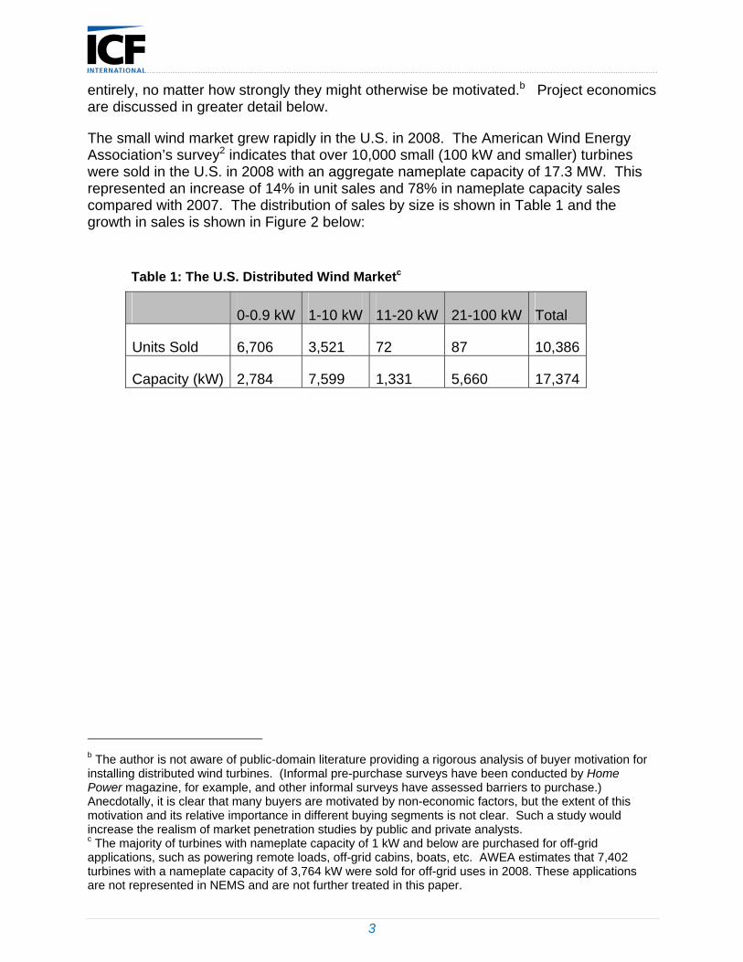
3
entirely, no matter how strongly they might otherwise be motivated.b Project economics are discussed in greater detail below.
The small wind market grew rapidly in the U.S. in 2008. The American Wind Energy Association’s survey2 indicates that over 10,000 small (100 kW and smaller) turbines were sold in the U.S. in 2008 with an aggregate nameplate capacity of 17.3 MW. This represented an increase of 14% in unit sales and 78% in nameplate capacity sales compared with 2007. The distribution of sales by size is shown in Table 1 and the growth in sales is shown in Figure 2 below:
Table 1: The U.S. Distributed Wind Marketc
0-0.9 kW 1-10 kW 11-20 kW 21-100 kW Total
Units Sold 6,706 3,521 72 87 10,386
Capacity (kW) 2,784 7,599 1,331 5,660 17,374
b The author is not aware of public-domain literature providing a rigorous analysis of buyer motivation for installing distributed wind turbines. (Informal pre-purchase surveys have been conducted by Home Power magazine, for example, and other informal surveys have assessed barriers to purchase.) Anecdotally, it is clear that many buyers are motivated by non-economic factors, but the extent of this motivation and its relative importance in different buying segments is not clear. Such a study would increase the realism of market penetration studies by public and private analysts. c The majority of turbines with nameplate capacity of 1 kW and below are purchased for off-grid applications, such as powering remote loads, off-grid cabins, boats, etc. AWEA estimates that 7,402 turbines with a nameplate capacity of 3,764 kW were sold for off-grid uses in 2008. These applications are not represented in NEMS and are not further treated in this paper.

4
Figure 2: Growth of the Small Wind Market in the U.S.3
3. Potential Market Size
The potential market for distributed wind is constrained by technical and economic factors.
3.1 Technical Factors
A proposed distributed wind project can be impaired by a number of different technical considerations. The most important is the availability of wind. A site with poor wind resources cannot support an economically viable wind project. Figure 2 below provides a coarse-scale representation of the country’s wind resources at a 50-meter hub height; the map displays Wind Power Classes, which are based on wind power density (Watts of wind power per square meter of rotor cross section).
Although it is not an ironclad rule, in general, if a site has a wind resource below Wind Power Class 3, it is unlikely to be economically successful. Almost 70% of the land surface in the Lower 48 states is in Wind Power Classes 1 and 2.4 At the lower hub heights used for the small to mid-scale turbines evaluated in this paper, the percentage of low-wind surface area is even higher.
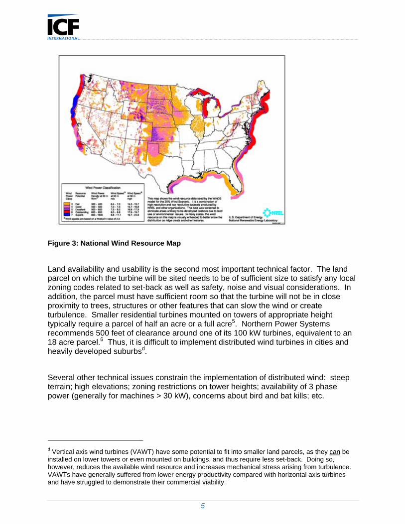
5
Figure 3: National Wind Resource Map
Land availability and usability is the second most important technical factor. The land parcel on which the turbine will be sited needs to be of sufficient size to satisfy any local zoning codes related to set-back as well as safety, noise and visual considerations. In addition, the parcel must have sufficient room so that the turbine will not be in close proximity to trees, structures or other features that can slow the wind or create turbulence. Smaller residential turbines mounted on towers of appropriate height typically require a parcel of half an acre or a full acre5. Northern Power Systems recommends 500 feet of clearance around one of its 100 kW turbines, equivalent to an 18 acre parcel.6 Thus, it is difficult to implement distributed wind turbines in cities and heavily developed suburbsd.
Several other technical issues constrain the implementation of distributed wind: steep terrain; high elevations; zoning restrictions on tower heights; availability of 3 phase power (generally for machines > 30 kW), concerns about bird and bat kills; etc.
d Vertical axis wind turbines (VAWT) have some potential to fit into smaller land parcels, as they can be installed on lower towers or even mounted on buildings, and thus require less set-back. Doing so, however, reduces the available wind resource and increases mechanical stress arising from turbulence. VAWTs have generally suffered from lower energy productivity compared with horizontal axis turbines and have struggled to demonstrate their commercial viability.
6
3.2 Economic Factors - Benefits
The financial analysis of a wind project includes the following factors:
Revenue from electricity generation. In most cases, the majority of the “revenue” from a distributed wind turbine’s electricity generation is actually the displacement of electric power deliveries by the electric utility. This displacement of electricity sales at relatively high retail rates is usually the largest single revenue source for a distributed wind turbine.e Any excess electricity above the site’s consumption can be sold the local electric utility, but the value of these sales varies dramatically. At a minimum, utilities are obliged to pay at least some proxy for wholesale electricity prices for electricity purchased from a customer/generator. In many states, excess generation of electricity above the site’s consumption can be sold back to the distribution utility at the full retail rate and excess generation from one month may be carried over to net against electricity purchases in subsequent months, often for up to a year. 7
Benefits from policy support. A variety of public policies provide additional benefits to distributed wind project owners:
o Federal tax benefits. At the Federal level, tax benefits are available to distributed wind turbine owners. The most important is the recently-enhanced Investment Tax Credit (ITC). This credit is valued at 30% of the project’s installed cost, without any upper limit on the credit amount, and is available through December 31, 2016. Under Section 1603 of the American Recovery and Reinvestment Act, this tax credit can also be converted into an outright cash grant from the Treasury, which is particularly favorable for taxable entities that do not anticipate sufficient taxable income to take full advantage of the ITC and for entities that prefer the certainty of a cash grant in the near term to a tax credit taken during one or more subsequent tax years. This conversion option is available only if significant project efforts (5% of project costs) are made by December 31, 2010. Alternatively, a project may take advantage of the Production Tax Credit (PTC), worth approximately 2 cents per kWh when output is sold to an unrelated third party over a 10-year period. (For the majority of distributed wind projects, the ITC is more valuable than the PTC.) In addition, wind turbines are eligible for accelerated depreciation under the Modified Accelerated Cost Recovery System.8
o Direct spending benefits. Federal and State agencies provide incentives for distributed wind projects through a variety of programs. For example, the U.S. Department of Agriculture’s Rural Energy for America
e The valuation of displaced electricity requires some analysis. For residential customers with simple kWh meters, displaced electricity will be worth the full retail rate (less any fixed customer charge). For commercial/industrial customers whose tariffs include both capacity (kW) and energy (kWh) based charges, consideration needs to be given to the uncertainty as to whether the wind turbine will reliably reduce the kW-based charges, for example, by comparing the facility’s load profile against the likely power production profile of the turbine. Unlike photovoltaic technology in hot climates, distributed wind generation cannot be assumed to be peak-coincident. In reality, a distributed wind turbine may not reliably avoid the peak capacity charge at all, in which case its displacement value is limited to the energy component of the tariff.
7
Program offers grants for feasibility studies and renewable energy installations. Many states offer direct grants for distributed wind projects or production-based incentives.
o Renewable Energy Certificates (RECs). RECs can be understood to represent the positive environmental and fuel diversity attributes arising from the generation of each MWh of renewable electricity. RECs can be marketed separately from the electric commodity and are purchased by entities subject to state Renewable Portfolio Standards to satisfy their obligations under those programs (“mandatory RECs”). In addition, many electricity customers purchase RECs voluntarily to “green up” their electricity supply (“voluntary RECs”). A distributed wind project owner can choose to retain the RECs created by their project (to keep their own electricity supply “green”), or sell the RECs created by their project, or some combination of the two. REC sales can be a significant additional revenue stream for a distributed wind project.
o Other policy support. A variety of other policy tools are used to enhance the financial viability of distributed wind projects: government-sponsored low-interest loans, sales tax abatements, property tax abatements, state income tax credits and deductions, preferential feed-in/buy-back tariffs, etc. These policy tools evolve rapidly; refer to the Database of State Incentives for Renewables and Efficiency (DSIRE) for additional details.
3.3 Economic Factors - Costs
The most important cost component for a distributed wind project (60-80%) is the cost of the hardware: rotor, nacelle and tower. Transportation and installation costs (including labor, equipment rental, concrete, wiring, metering, interconnecting with the distribution utility, etc.) can be considerable (10-35%), particularly with taller towers, remoter sites and more difficult terrain. Pre-construction costs – feasibility analyses, project design, permitting, zoning, etc. -- may be modest for a rural residential project confronting limited zoning and permitting challenges, but run to tens of thousands of dollars for a commercial-scale project with more complex design and engineering requirements, and can account for 5-15% of initial project costs. In addition, turbine owners need to plan for annual operation and maintenance (O&M) costs, warranty expenses, as well as costs related to insurance, incremental property taxes (if any), and eventual decommissioning of the turbine when it reaches the end of its useful life.
Example capital costs for present-day distributed wind turbines are shown in Table 5; O&M costs are show in Table 7.
3.4 Market Potential - Conclusions
A recent analysis evaluated the technical and economic potential of existing mid-scale distributed wind projects in the 10-5000 kW size rangef. The analysis found that
f The study evaluated individual turbines up to 1000 kW as well as small community wind projects consisting of five 1000 kW turbines.
8
commercial, industrial and institutional buyers motivated purely by economics would purchase over 2700 10 kW turbines, about 10,000 50 kW turbines, approximately 200 100 kW turbines, and about 3500 250 kW turbines if 2008 incentive levels were assumed to remain unchanged for 10 years. 9
This study had some important limitations. It did not evaluate residential buyers in the 1-10 kW range. It also did not attempt to quantify market penetration driven by non-economic factors, such as the desire to reduce greenhouse gas emissions, even though anecdotal information suggests that non-economic factors are important drivers of distributed wind projects. In addition, the study was completed prior to the implementation of the uncapped 30% ITC, which can be expected to dramatically increase the number of viable projects.
This study also evaluated the impact of improving today’s mid-scale distributed wind turbines. Longer blades, taller towers, greater productivity (particularly at low wind speeds), and lower costs combined to increase the potential market for 250 and 500 kW turbines by a factor of 25 or more.10
A second study provides market potential estimates based on technology application:
Table 2: Market Projections of Grid-Connected Domestically Installed Wind Turbines11
Cumulative Units Installed
Residential (1-25 kW) Farm, Business, Industrial (10-400 kW)
2005 1,800 20
2010 6,250 1,270
2015 14,000 4,270
2020 36,500 7,395
4. Performance Objectives
Ideally, a wind turbine would extract the maximum amount of kinetic energy from the wind at the lowest possible cost. However, wind turbines, like all other goods, represent a set of compromises to satisfy multiple goals. These include:
1. Energy productivity: Turbines vary in their ability to extract energy from the wind, and all other things being equal, a turbine that produces more energy from a given wind resource is more valuable than a turbine that produces less. This can be achieved by using longer blades, more efficient blade design, more efficient transmission (or direct drive), a more efficient generator/alternator, better yaw control, etc. The turbine’s behavior over a dynamic range is also a critical factor: turbines can be designed to start spinning at lower speeds, to produce more energy at the most frequent wind speeds, or to continue producing at higher wind speeds, but it is difficult to design a turbine that can do all three.
9
Because wind is variable at a given site and even more variable across many sites, no one turbine model is optimal for every site.
2. Project Cost: Turbines are expensive, and manufacturers seek out ways to reduce costs. This can include using less-expensive materials, improving manufacturing techniques, sourcing less-expensive components, and improving the efficiency of distribution and installation. Volume is an important determinant: many turbine models in the 1-250 kW range are produced in limited quantities, which drives up unit costs. Larger production runs give the manufacturer more leverage in negotiating with upstream suppliers, and permits more investment in production tooling.
3. Overspeed Control: Once the turbine is producing at its maximum output, any further increase in wind speed is essentially “wasted” from a power generation perspective and at very high speed can cause structural damage to the turbine. Turbines use a variety of methods to regulate turbine loading and rotational speed: by furling the rotor towards the tail vane (thereby reducing the rotor cross-section presented to the wind), deploying various types of blade-mounted brakes, changing the blade pitch, stalling, and/or by electrical braking.
4. Tower Height and Cost: In most terrains, wind speed increases with height, at least for tens of meters. Tall towers improve cost-effectiveness in most areas. Some turbines are available on tilt-up towers, while others can only be mounted on fixed towers. For fixed towers, erection costs increase as tower height increases. Taller towers also make maintenance visits more hazardous and time-consuming, driving up O&M costs.
5. Reliability/Durability: Utility-scale wind farms can afford to have on-site technicians to provide regular maintenance and repair services. A single distributed wind turbine at a home or business cannot be expected to receive the same level of attention, and therefore should be designed and built to minimize maintenance requirements. (Some level of maintenance will always be required.) Although wind turbines have few moving parts, they are subjected to significant stresses and vibration from winds that vary in speed and direction. The rotor and drivetrain is expected to spin hundreds of times per minute with blade tip speeds of over 100 mph, and this performance is expected to last for decades. To reduce maintenance costs, production degradation and downtime, the turbine should be built with well-engineered components fabricated from long-lasting materials. However, this drives up costs. Lower rotor speeds can increase longevity, but at the cost of reduced energy production.
6. Noise: Several design choices that increase energy productivity (longer blades, higher rotational speed, and certain overspeed controls, such as furling) increase the sound pressure produced by the turbine. This tradeoff can be particularly objectionable for distributed wind turbines as they are ordinarily sited close to homes and businesses.
NEMS “builds” distributed generation (DG) in future years based on how cost-effective the technologies are. NEMS incorporates a 30-year discounted cash flow model that assesses the internal rate of return (IRR) of various DG technologies; NEMS then uses the IRR and a learning function model to forecast the technology’s penetration in the
10
marketplace. Other thing being equal, if a DG technology’s IRR increases in a future year, it will penetrate the market further than if its IRR remains unchanged or falls.12
Of the key performance objectives listed above, only the turbine’s cost and performance figure into the IRR calculation. Overspeed control, reliability/durability and noise are not considered. In the real world, however, these parameters are part of the turbine design process, and manufacturers make necessary compromises to ensure that turbines perform safely and reliably over the long run. The cost and performance projections presented later in this paper were developed under the assumption that manufacturers would continue to balance multiple objectives in the future as they have done in the past.
It is also important to note that NEMS only considers decisions made on economic grounds; the model does not endogenously account for turbines installed for reasons other than economics.
5. Interpreting Performance Data for Distributed Wind Technology
Distributed wind technology performance data needs to be interpreted with care. The challenge arises partly from a lack of industry standardization, partly from the highly site-specific performance of wind turbines, and partly because some manufacturers provide inaccurate or incomplete data to their buyers.
Industry standardization. Until very recently, the distributed wind industry lacked standardized terminology, test methods or product certification processes. Rated capacity, for example, is a less meaningful metric than it may seem. Manufacturers choose the wind speed at which they rate their turbines’ capacity, and as noted in Table 4, the values can vary considerably. This makes it difficult to make an “apples to apples” comparison of two turbines even of the same nominal rated capacity; one may be rated based on an 11 m/s wind, for example, while another is rated at 14 m/s.
Lack of industry standardization should begin to recede as an issue in the near future. The American Wind Energy Association (AWEA) published a performance and safety standard for small wind turbinesg in late 2009 that established specific test methods for various performance parameters, including rated capacity, annual energy production, and noise.13 For example, the standard established that a turbine’s capacity should be rated at a wind speed of 11 m/s.
In addition, 2010 will see the Small Wind Certification Council commence operations. The SWCC is an independent organization that will certify turbine testing conducted in accordance with the AWEA small wind turbine standard, provide an SWCC label to certified turbines, and provide test results on its web site.14 The combination of standardized test methods and independent certification of testing results will make a material contribution to improving the usefulness of turbine performance data.
g The standard applies to turbines with swept areas of 200 square meters, or a rotor diameter of about 16m. This translates to a nominal capacity of about 65 kW.
11
Site-specific data. Although a turbine’s rated capacity is often the first point of reference, in fact, the most important metric for a wind project is the turbine’s estimated annual energy production (AEP) for the project site. This metric drives the project’s potential revenue much more directly than rated capacity does. To estimate AEP, it is necessary to know the following information:
The project’s hub height; The wind resource distribution: how many hours per year the wind blows
within specific speed ranges (bins) at the project’s hub height; Turbulence at the project’s hub height due to nearby trees, buildings and
other obstructions; The turbine’s production curve: how many kWh the turbine produces for
each specific wind speed bin. The turbine’s expected availability and losses (e.g., line losses)
For large, utility scale projects, it is typical to measure the wind resource at hub height at multiple points across the development area for at least a year-long period, and then to use sophisticated software to estimate the effects of terrain and of the turbine array itself on AEP for each turbine. Distributed wind projects in the 1-100 kW range rarely utilize such a data-intensive approach, usually only at the upper end of the range. Instead, homeowners, turbine dealers and project developers rely on a combination of coarse-scale wind maps (themselves derived from extensive modeling) and manufacturer-supplied production curve data.
It is not uncommon for this approach to result in significant mis-estimation of AEP. To start with, the typical state-level coarse-scale wind map is merely a starting point for wind estimation. Actual wind conditions within each of the map’s raster cells can vary dramatically. Second, even assuming that the map provides an accurate estimate of the wind resource at a specific site, the map may be estimating wind resources at one height (e.g., a 50-meter hub height), but the turbine may be mounted at a different height (e.g., 30 meters, where wind power is substantially less). Or turbulence caused by site conditions (e.g., nearby buildings or large trees) may be ignored, although it can have a powerful effect on turbine performance.
A third factor is incorrect or incomplete information supplied by manufacturers, particularly the turbine’s power curve. (See Table 3 below.) For example, one widely-used distributed wind turbine (Turbine A) has recently undergone independent testing at NREL. Comparing NREL’s measured data with manufacturer literature indicates that the manufacturer overstates AEP by 71% at the AWEA reference speed of 5 m/s. The differences between NREL’s measured data and manufacturer literature data were somewhat lower at higher wind speeds, falling to a 25% difference at an 8 m/s annual average wind speed for this turbine. Note, however, that the literature associated with Turbine B goes to some lengths to qualify potential turbulence factors at various wind speeds (e.g., hedges, windbreaks, buildings) and appears to have adjusted its AEP values accordingly.15

12
Table 3: Percentage Difference between Manufacturer Literature and NREL Test Datah
Average Annual Wind Speed
Wind Turbine A Wind Turbine B Wind Turbine C
4 m/s NA NA 46%
5 m/s 71% -23% 26%
6 m/s 43% -24% 9%
7 m/s 31% NA NA
8 m/s 25% NA NA
Manufacturers and dealers may also deemphasize noise considerations or fail to educate the buyer on the desirability of (or need for) a tall tower. The advent of the AWEA small wind standard and the SWCC will make it easier for buyers to obtain accurate and meaningful information, but only education will ensure that buyers get the most value from their significant investment in distributed wind.
6. Data Issues – Implications for NEMS
NEMS “builds” distributed wind turbines in Census divisions, which are then overlaid with an NREL wind map. NEMS refers to the geographical overlay of a Census division and wind map polygon as a “niche”. For each niche, NEMS estimates the distribution of wind speeds using a Weibull k of 2 and a wind shear exponent of 0.2.
The model then estimates AEP by applying a turbine’s rated capacity across a cubic power equation.
This method is vulnerable to the following sources of error:
The wind resource map may not be appropriate for the turbine’s hub height;
The wind speed distribution may not be appropriate in light of the topography of the niche;
The varying altitude across the niches may not be appropriately incorporated into the computations;
Turbulence may not be appropriately represented; The nominal power curve may not be appropriate for other specific
turbines; Scaling the AEP based on ratios of rated capacity may not be appropriate
in view of the inconsistency of capacity rating methods. h Values represent the difference between the manufacturer’s data and NREL’s data, divided by the NREL data. Positive differences indicate that manufacturer AEP data are higher than NREL AEP data for the same average annual wind speed. Manufacturer data for Turbines B and C were not available for unit values of m/s and were interpolated from values expressed in half meters per second (e.g., 4.5 m/s, 5.5 m/s, etc.) using a simple average.
13
Going forward, the author recommends that EIA take the following steps to increase the realism of its modeling efforts:
1. Verify that the national wind map corresponds to the hub heights of the typical distributed wind turbine, for example 30-40 meters.
2. Consider whether to vary the Weibull k and wind shear exponent based on the land surface and altitude within the niche.
3. Altitude and turbulence factors could also be more directly represented (e.g. the decrease in air pressure at higher altitudes will decrease the energy output for a wind turbine at a lower altitude, all other things being equal).
4. As soon as it becomes available in quantity, use AWEA-standard AEP data that have been certified by the SWCC for the base year, and use these data to interpolate the AEP for other turbine sizes that have not yet been certified by SWCC.
5. Until SWCC data become available: a. use manufacturer-supplied AEP data for the base year, but derate these
data to reflect the discrepancies described in Table 3 above. b. apply the adjusted AEP data to specific sites, and further modify the data
to reflect local wind resources, altitude, Weibull k, and wind shear exponent.
7. Technology Baseline
Cost and dimensional data for baseline distributed wind technology are represented in Tables 4 and 5 below. The turbines chosen for this table were selected to represent a range of project capacities and are popular models within their respective size classes. Note that each turbine’s rated capacity is derived from a different reference wind speed.
Table 4: Dimensional Data for Selected Distributed Wind Turbines
TypicalRated Rated Wind Rotor Tower
Capacity Speed Diameter HeightManufacturer Model (kW) (m/s) (m) (m)
Southwest Windpower Skystream 3.7 2.4 13 3.7 26Bergey BWC XL-S 10 14 7 37Entegrity EW50 50 11.3 15 37Northern Power Systems Northwind 100 100 14.5 21 37
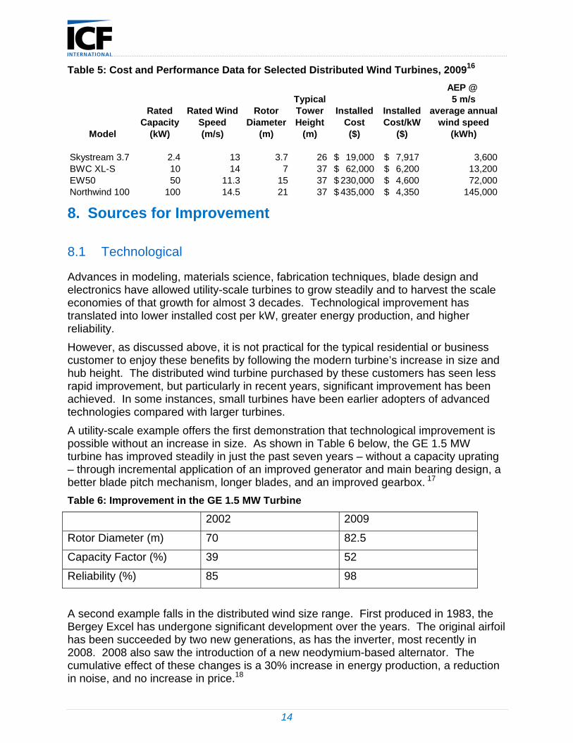
14
Table 5: Cost and Performance Data for Selected Distributed Wind Turbines, 200916
AEP @ Typical 5 m/s
Rated Rated Wind Rotor Tower Installed Installed average annualCapacity Speed Diameter Height Cost Cost/kW wind speed
Model (kW) (m/s) (m) (m) ($) ($) (kWh)
Skystream 3.7 2.4 13 3.7 26 19,000$ 7,917$ 3,600 BWC XL-S 10 14 7 37 62,000$ 6,200$ 13,200 EW50 50 11.3 15 37 230,000$ 4,600$ 72,000 Northwind 100 100 14.5 21 37 435,000$ 4,350$ 145,000
8. Sources for Improvement
8.1 Technological
Advances in modeling, materials science, fabrication techniques, blade design and electronics have allowed utility-scale turbines to grow steadily and to harvest the scale economies of that growth for almost 3 decades. Technological improvement has translated into lower installed cost per kW, greater energy production, and higher reliability.
However, as discussed above, it is not practical for the typical residential or business customer to enjoy these benefits by following the modern turbine’s increase in size and hub height. The distributed wind turbine purchased by these customers has seen less rapid improvement, but particularly in recent years, significant improvement has been achieved. In some instances, small turbines have been earlier adopters of advanced technologies compared with larger turbines.
A utility-scale example offers the first demonstration that technological improvement is possible without an increase in size. As shown in Table 6 below, the GE 1.5 MW turbine has improved steadily in just the past seven years – without a capacity uprating – through incremental application of an improved generator and main bearing design, a better blade pitch mechanism, longer blades, and an improved gearbox. 17
Table 6: Improvement in the GE 1.5 MW Turbine
2002 2009
Rotor Diameter (m) 70 82.5
Capacity Factor (%) 39 52
Reliability (%) 85 98
A second example falls in the distributed wind size range. First produced in 1983, the Bergey Excel has undergone significant development over the years. The original airfoil has been succeeded by two new generations, as has the inverter, most recently in 2008. 2008 also saw the introduction of a new neodymium-based alternator. The cumulative effect of these changes is a 30% increase in energy production, a reduction in noise, and no increase in price.18
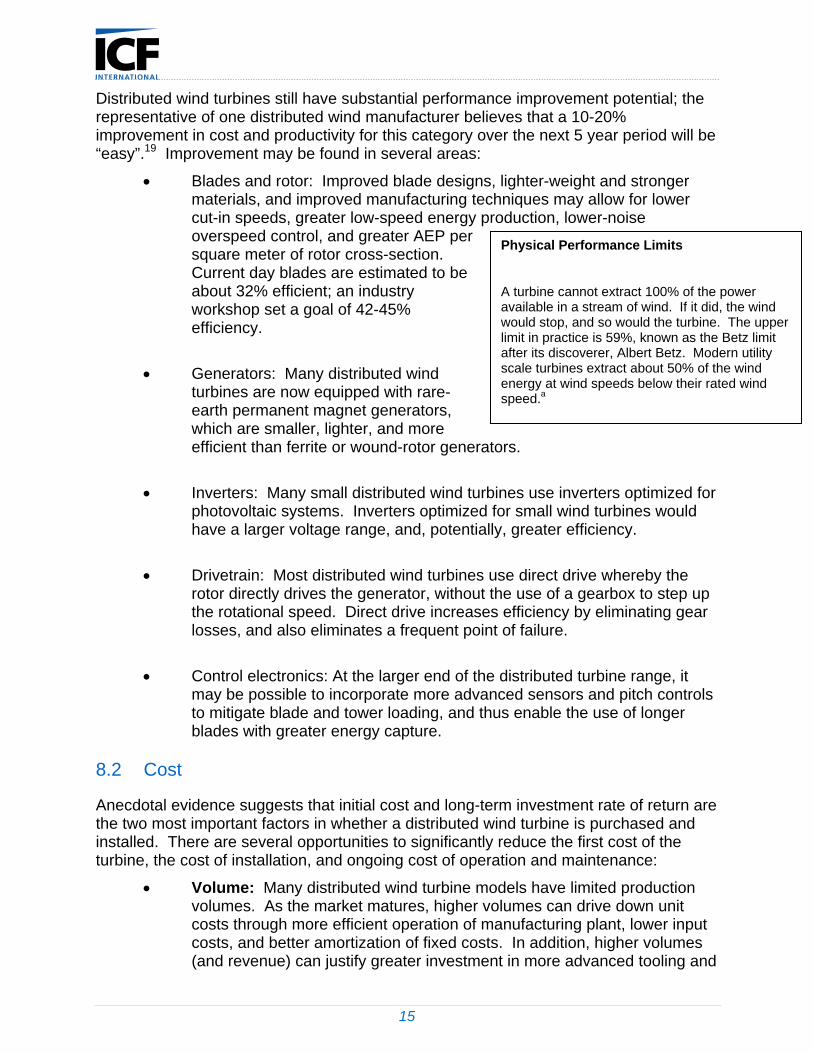
15
Distributed wind turbines still have substantial performance improvement potential; the representative of one distributed wind manufacturer believes that a 10-20% improvement in cost and productivity for this category over the next 5 year period will be “easy”.19 Improvement may be found in several areas:
Blades and rotor: Improved blade designs, lighter-weight and stronger materials, and improved manufacturing techniques may allow for lower cut-in speeds, greater low-speed energy production, lower-noise overspeed control, and greater AEP per square meter of rotor cross-section. Current day blades are estimated to be about 32% efficient; an industry workshop set a goal of 42-45% efficiency.
Generators: Many distributed wind turbines are now equipped with rare-earth permanent magnet generators, which are smaller, lighter, and more efficient than ferrite or wound-rotor generators.
Inverters: Many small distributed wind turbines use inverters optimized for photovoltaic systems. Inverters optimized for small wind turbines would have a larger voltage range, and, potentially, greater efficiency.
Drivetrain: Most distributed wind turbines use direct drive whereby the rotor directly drives the generator, without the use of a gearbox to step up the rotational speed. Direct drive increases efficiency by eliminating gear losses, and also eliminates a frequent point of failure.
Control electronics: At the larger end of the distributed turbine range, it may be possible to incorporate more advanced sensors and pitch controls to mitigate blade and tower loading, and thus enable the use of longer blades with greater energy capture.
8.2 Cost
Anecdotal evidence suggests that initial cost and long-term investment rate of return are the two most important factors in whether a distributed wind turbine is purchased and installed. There are several opportunities to significantly reduce the first cost of the turbine, the cost of installation, and ongoing cost of operation and maintenance:
Volume: Many distributed wind turbine models have limited production volumes. As the market matures, higher volumes can drive down unit costs through more efficient operation of manufacturing plant, lower input costs, and better amortization of fixed costs. In addition, higher volumes (and revenue) can justify greater investment in more advanced tooling and
Physical Performance Limits
A turbine cannot extract 100% of the power available in a stream of wind. If it did, the wind would stop, and so would the turbine. The upper limit in practice is 59%, known as the Betz limit after its discoverer, Albert Betz. Modern utility scale turbines extract about 50% of the wind energy at wind speeds below their rated wind speed.a
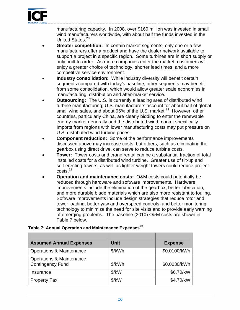
16
manufacturing capacity. In 2008, over $160 million was invested in small wind manufacturers worldwide, with about half the funds invested in the United States.20
Greater competition: In certain market segments, only one or a few manufacturers offer a product and have the dealer network available to support a project in a specific region. Some turbines are in short supply or only built-to-order. As more companies enter the market, customers will enjoy a greater choice of technology, shorter lead times, and a more competitive service environment.
Industry consolidation: While industry diversity will benefit certain segments compared with today’s baseline, other segments may benefit from some consolidation, which would allow greater scale economies in manufacturing, distribution and after-market service.
Outsourcing: The U.S. is currently a leading area of distributed wind turbine manufacturing; U.S. manufacturers account for about half of global small wind sales, and about 95% of the U.S. market.21 However, other countries, particularly China, are clearly bidding to enter the renewable energy market generally and the distributed wind market specifically. Imports from regions with lower manufacturing costs may put pressure on U.S. distributed wind turbine prices.
Component reduction: Some of the performance improvements discussed above may increase costs, but others, such as eliminating the gearbox using direct drive, can serve to reduce turbine costs.
Tower: Tower costs and crane rental can be a substantial fraction of total installed costs for a distributed wind turbine. Greater use of tilt-up and self-erecting towers, as well as lighter weight towers could reduce project costs.22
Operation and maintenance costs: O&M costs could potentially be reduced through hardware and software improvements. Hardware improvements include the elimination of the gearbox, better lubrication, and more durable blade materials which are also more resistant to fouling. Software improvements include design strategies that reduce rotor and tower loading, better yaw and overspeed controls, and better monitoring technology to minimize the need for site visits and to provide early warning of emerging problems. The baseline (2010) O&M costs are shown in Table 7 below.
Table 7: Annual Operation and Maintenance Expenses23
Assumed Annual Expenses Unit Expense
Operations & Maintenance $/kWh $0.0100/kWh
Operations & Maintenance Contingency Fund $/kWh $0.0030/kWh
Insurance $/kW $6.70/kW
Property Tax $/kW $4.70/kW
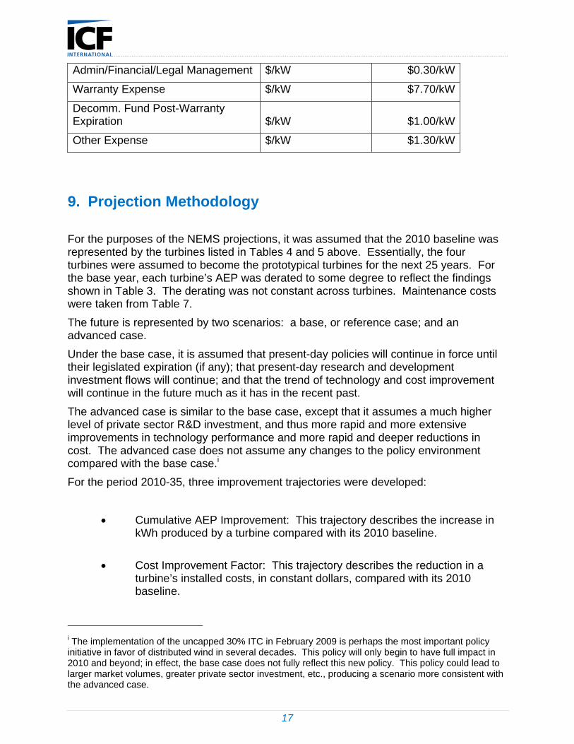
17
Admin/Financial/Legal Management $/kW $0.30/kW
Warranty Expense $/kW $7.70/kW
Decomm. Fund Post-Warranty Expiration $/kW $1.00/kW
Other Expense $/kW $1.30/kW
9. Projection Methodology
For the purposes of the NEMS projections, it was assumed that the 2010 baseline was represented by the turbines listed in Tables 4 and 5 above. Essentially, the four turbines were assumed to become the prototypical turbines for the next 25 years. For the base year, each turbine’s AEP was derated to some degree to reflect the findings shown in Table 3. The derating was not constant across turbines. Maintenance costs were taken from Table 7.
The future is represented by two scenarios: a base, or reference case; and an advanced case.
Under the base case, it is assumed that present-day policies will continue in force until their legislated expiration (if any); that present-day research and development investment flows will continue; and that the trend of technology and cost improvement will continue in the future much as it has in the recent past.
The advanced case is similar to the base case, except that it assumes a much higher level of private sector R&D investment, and thus more rapid and more extensive improvements in technology performance and more rapid and deeper reductions in cost. The advanced case does not assume any changes to the policy environment compared with the base case.i
For the period 2010-35, three improvement trajectories were developed:
Cumulative AEP Improvement: This trajectory describes the increase in kWh produced by a turbine compared with its 2010 baseline.
Cost Improvement Factor: This trajectory describes the reduction in a turbine’s installed costs, in constant dollars, compared with its 2010 baseline.
i The implementation of the uncapped 30% ITC in February 2009 is perhaps the most important policy initiative in favor of distributed wind in several decades. This policy will only begin to have full impact in 2010 and beyond; in effect, the base case does not fully reflect this new policy. This policy could lead to larger market volumes, greater private sector investment, etc., producing a scenario more consistent with the advanced case.

18
O&M Factor: This trajectory describes the reduction in annual O&M costs compared with the 2010 baseline.
Table 8: Assumptions for the Base and Advanced Cases
Cumulative AEP Improvement
Factor vs. 2010
Cost Improvement
Factor vs. 2010
O&M Factor vs. 2010
Base Advanced Base Advanced Base Advanced
2015 10% 12% -8% -10% 0.98 0.97
2020 18% 21% -13% -14% 0.96 0.94
2025 23% 28% -16% -18% 0.94 0.92
2030 26% 33% -18% -21% 0.92 0.90
2035 28% 36% -20% -24% 0.90 0.88
Other assumptions include:
Capacity factor: As noted above, the authors recommend using AEP as the key metric of energy performance. However, the accompanying data table provides calculated capacity factors for different turbines over the projection horizon by turbine size, year and scenario.
Equipment life: A 25 year life was assumed for both scenarios.
Availability: We assume 98% availability in both scenarios.
O&M Costs: Summing the values in Table 7 yields an annual O&M factor based partly on capacity ($21.70/kW-year) and partly on energy production ($0.013/kWh).
19
Endnotes
1 http://www.industry.nsw.gov.au/energy/sustainable/renewable/wind
2 AWEA, Small Wind Turbine Global Market Study: Year Ending 2008.
3 Ibid, p. 5.
4 Kwartin et al., An Analysis of the Technical and Economic Potential for Mid-Scale Distributed Wind, NREL, December 2008, p. 41.
5 Southwest Windpower, “Skystream 3.7: 2.4 kW Residential Power Appliance”.
6 http://www.northernpower.com/wind-power-basics/faq.php#WhatMakesAGoodWindSite
7 http://dsireusa.org/summarytables/rrpre.cfm
8 Ibid.
9 Kwartin et al., p. 54
10 Kwartin et al., p. 61
11 Forsyth, T., and Baring-Gould, I., “Distributed Wind Market Applications,” NREL, November 2007, p. 5.
12 DOE, Commercial Sector Demand Module of the National Energy Modeling System: Model Documentation 2009, DOE/EIA-M066(2009), May 2009, pp 40-44.
13 American Wind Energy Association, AWEA Small Wind Turbine Performance and Safety Standard, (AWEA Standard 9.1 – 2009) © The American Wind Energy Association, 2009.
14 http://www.smallwindcertification.org/index.html
15 Smith, Joe, “NREL Small Wind Technology Update,” AWEA Small & Community Wind Conference & Exhibition, November 5, 2009, Detroit, MI, and manufacturer literature.
16 Sagrillo, Mick, “Size Matters!” Windletter, 28(3); AEP data:
a. Bergey Skystream 3.7, 3-CMLT-1338-01 REV F 1-09
b. “Power Your Dream With the Wind”, Bergey Windpower, accessed May 2010.
20
c. “Entegrity Wind Systems: Commercial Wind Energy Provider and Manufacturer of the EW50”, 2009.
d. “Northwind 100: Community Scale Wind Turbine”, Northern Power Systems, 2009.
17 Frick, Bob, untitled presentation, AWEA Small & Community Wind Conference & Exhibition, November 5, 2009, Detroit, MI.
18 Wilke, Steve, “The Evolution of the Bergey Excel wind turbine,” AWEA Small & Community Wind Conference & Exhibition, November 5, 2009, Detroit, MI.
19 Kruse, Andy, personal communication, AWEA Small & Community Wind Conference & Exhibition, November 5, 2009, Detroit, MI.
20 AWEA, Small Wind Turbine Global Market Study: Year Ending 2008, p. 10.
21 Ibid, p. 15.
22 U.S. Department of Energy, 20% Wind Energy by 2030: Meeting the Challenges, Proceedings of the Workshop, October 6-7, 2008, pp. 13-25.
23 Kwartin et al., pp. 33-34, for commercial/industrial turbines and unpublished data for residential turbines. Values in Table 7 represent a 2/3 weighting for residential scale turbines and a 1/3 weighting for commercial/industrial scale turbines.
Bibliography
Abundant Renewable Energy. (2008, October 28). Wind Energy Systems from
Abundant Renewable Energy [Brochure]. Newberg, OR: Abundant Renewable
Energy.
American Wind Energy Association. (2009). AWEA Small Wind Turbine Global Market
Study: Year Ending 2008. Retrieved from
http://www.awea.org/smallwind/pdf/09_AWEA_
Small_Wind_Global_Market_Study.pdf
American Wind Energy Association. (2009) AWEA Small Wind Turbine Performance
and Safety Standard (AWEA Standard 9.1 – 2009). Washington, DC: American
Wind Energy Association.
American Wind Energy Association. (2002, June). The U.S. Small Wind Turbine
Industry Roadmap: A 20-year Industry Plan for Small Wind Turbine Technology.
Retrieved from http://www.awea.org/smallwind/documents/31958.pdf
Bergey Wind Company. (2010a). BWC XL.1: 1 kW Class Wind Turbine [Brochure].
Norman, OK: Bergey Wind Company.
Bergey Wind Company. (2010b). BWC Excel: 10 kW Class Wind Turbine [Brochure].
Norman, OK: Bergey Wind Company.
Blair, N, M. Hand, W. Short, & P. Sullivan. (2008, June). Modeling Sensitivities to the
20% Wind Scenario Report with the WinDS Model (Report No. NREL/CP-670-
43511). Retrieved from http://www.nrel.gov/docs/fy08osti/43511.pdf

Bolinger, M. (2009, May 5). An Update on U.S. Wind Power Prices and Factors that
Influence Them [Presentation]. WindPower 2009, Chicago, IL.
Department of Energy. (2009, October). Commercial Sector Demand Module of the
National Energy Modeling System: Model Documentation 2009 (Report No.
DOE/EIA-M066). Retrieved from
http://www.eia.doe.gov/oiaf/aeo/overview/commercial.html
Entegrity Wind Systems Inc. (2009). Commercial Wind Energy Provider and
Manufacturer of the EW50 [Brochure]. Boulder, CO: Entegrity Wind Systems Inc.
Frick, B. (2009, November 5). [Presentation]. AWEA Small & Community Wind
Conference & Exhibition, Detroit, MI.
Forsyth, T. (2008). Small (Distributed) Wind Technology [Presentation]. WindPower
2008, Houston, TX.
Forsyth, T. & I. Baring-Gould. (2007). Distributed Wind Market Applications (Report No.
NREL/TP-500-39851). Retrieved from http://www.nrel.gov/docs/fy08osti/39851.pdf
Gaia-Wind. (2010). Gaia-Wind 11 kW, Energy Production Data [Brochure]. Glasgow,
United Kingdom: Gaia-Wind.
GE Energy. (2009, November 5). Turbine Technology, Construction & Operation
[Presentation]. AWEA Small & Community Wind Conference & Exhibition, Detroit,
MI.
Gipe, P. (n.d.) Small and Household-size Wind Turbines. Retrieved from
http://www.wind-
works.org/articles/small_turbines.html#Small%20Turbine%20Product%20Reviews
Goldsmith, D. (2009, November 4). Advanced Small Wind Turbine Technology
[Presentation]. AWEA Small & Community Wind Conference & Exhibition, Detroit,
MI.
Government of New South Wales, Department of Industry and Investment. (2010,
March 24). Energy: Wind Power. Retrieved from
http://www.industry.nsw.gov.au/energy/ sustainable/renewable/wind
Kruse, Andy. (n.d.) Introduction to the Residential Wind Industry [Brochure]. Flagstaff,
AZ: Southwest Windpower, Inc.
Kwartin, R., A. Wolfrum, K. Granfield, A. Kagel, & A. Appleton (2008). An Analysis of the
Technical and Economic Potential for Mid-Scale Distributed Wind (Report No.
NREL/SR-500-44280). Retrieved from National Renewable Energy Laboratory:
http://www.nrel.gov/ wind/pdfs/midscale_analysis.pdf
Northern Power Systems. (2009) Wind Power: Frequently Asked Questions. Retrieved
from http://www.northernpower.com/windpowerbasics/faq.php#WhatMakesAGood
WindSite
Northwind. (2010a). Northwind 100 Specifications [Brochure]. Barre, VT: Northwind
Northwind. (2010b). Northwind 100 Community Scale Wind Turbine [Brochure]. Barre,
VT: Northwind
Sagrillo, Mick. (2009). Size Matters! Windletter, 28(3), 1-6. Retrieved from
http://www.renewwisconsin.org/wind/Toolbox-Homeowners/Size%20Matters.pdf
Small Wind Certification Council. (2009, November 3). Policy Summary-SWCC
Certification of Small Wind Turbines [Presentation]. AWEA Small & Community Wind
Conference & Exhibition, Detroit, MI.
Small Wind Certification Council. (n.d.). Small Wind Certification Council. Retrieved
March 24, 2010, from http://www.smallwindcertification.org/index.html
Smith, J. (2009, November 5). NREL Small Wind Technology Update [Presentation].
AWEA Small & Community Wind Conference & Exhibition, Detroit, MI.
Southwest Windpower. (2010). Skystream 3.7: 2.4 kW Residential Power Appliance
[Brochure]. Flagstaff, AZ: Southwest Windpower.
U.S. Department of Energy. (2008, October 6-7). 20% Wind Energy by 2030: Meeting
the Challenges. Proceedings of Workshop.
U.S. Department of Energy, Database of State Incentives for Renewables & Efficiency.
(2009). Rules, Regulations & Policies for Renewable Energy. Retrieved from
http://dsireusa.org/ summarytables/rrpre.cfm
U.S. Department of Energy, Energy Efficiency and Renewable Energy. (2008, May).
20% Wind Energy by 2030: Increasing Wind Energy’s Contributions to U.S.
Electricity Supply (Prepublication Version). Retrieved from
http://www.nrel.gov/docs/fy08osti/41869.pdf

Wilkie, S. (2009, November 5). The Evolution of the Bergey Excel wind turbine
[Presentation]. AWEA Small & Community Wind Conference & Exhibition, Detroit,
MI.
Wiser, R. & M. Bolinger. (2009, July). 2008 Wind Technologies Market Report.
Retrieved from http://eetd.lbl.gov/ea/EMS/reports/2008-wind-technologies.pdf

Headquarters
ICF International
9300 Lee Highway
Fairfax, Virginia 22031
www.icfi.com