distributed network protocols lecture notes
TRANSCRIPT

Distributed Network Protocols
Lecture Notes1
Prof. Adrian Segall
Department of Electrical Engineering
Technion, Israel Institute of Technology
segall at ee.technion.ac.il
and
Department of Computer Engineering
Bar Ilan University
Adrian.Segall at biu.ac.il
March 13, 2013
1Thanks are due to Lior Shabtay for producing and solving many of the problems

March 13, 2013
c©Adrian Segall 2

Contents
1 Introduction 7
2 DATA-LINK CONTROL PROTOCOLS 9
2.1 The Model . . . . . . . . . . . . . . . . . . . . . . . . . . . . . . . . . . . . . . . . . . . . . . 10
2.2 The Alternating Bit Protocol . . . . . . . . . . . . . . . . . . . . . . . . . . . . . . . . . . . . 12
2.3 Sliding-Window DLC Procedures . . . . . . . . . . . . . . . . . . . . . . . . . . . . . . . . . 20
2.4 Link Initialization Procedures . . . . . . . . . . . . . . . . . . . . . . . . . . . . . . . . . . . 30
2.4.1 The HDLC LI Procedure . . . . . . . . . . . . . . . . . . . . . . . . . . . . . . . . . . 31
2.4.2 Link Initialization Procedures that Ensure Synchronization . . . . . . . . . . . . . . . 34
2.4.3 Unbalanced LI Procedures that Ensure Synchronization . . . . . . . . . . . . . . . . 34
2.4.4 A Function-Assigning LI-Procedure . . . . . . . . . . . . . . . . . . . . . . . . . . . . 40
2.4.5 A Balanced LI Procedure . . . . . . . . . . . . . . . . . . . . . . . . . . . . . . . . . . 42
2.5 CONCLUSIONS . . . . . . . . . . . . . . . . . . . . . . . . . . . . . . . . . . . . . . . . . . . 45
3 PI-TYPE NETWORK PROTOCOLS 47
3.1 The Fixed Topology Model . . . . . . . . . . . . . . . . . . . . . . . . . . . . . . . . . . . . . 48
3.2 The Variable Topology Model . . . . . . . . . . . . . . . . . . . . . . . . . . . . . . . . . . . 50
3.3 Basic Protocols . . . . . . . . . . . . . . . . . . . . . . . . . . . . . . . . . . . . . . . . . . . 52
3.3.1 Propagation of Information (PI) . . . . . . . . . . . . . . . . . . . . . . . . . . . . . 52
3.3.2 Propagation of Information with Feedback (PIF) . . . . . . . . . . . . . . . . . . . . 56
3.4 Repeated Propagations of Information (RPI) . . . . . . . . . . . . . . . . . . . . . . . . . . . 62
3.5 Multi-Initiator Propagation of Information (MPI) - Reset Protocols . . . . . . . . . . . . . . 70
3.6 Multi-Initiator Propagation of Information-Topological changes (EMPIF) . . . . . . . . . . . 82
3.7 Generalized PIF (GPIF) . . . . . . . . . . . . . . . . . . . . . . . . . . . . . . . . . . . . . . 93
3.7.1 Distributed Snapshots (DS) . . . . . . . . . . . . . . . . . . . . . . . . . . . . . . . . 95
3.7.2 The Echo Protocol . . . . . . . . . . . . . . . . . . . . . . . . . . . . . . . . . . . . . 96
3.7.3 Termination Detection for Diffusing Computations (TDDC) . . . . . . . . . . . . . . 98
3.7.4 Termination Detection for Diffusing Computations - Version 2 . . . . . . . . . . . . . 100
3.7.5 Synchronizers . . . . . . . . . . . . . . . . . . . . . . . . . . . . . . . . . . . . . . . . 100
4 CONNECTIVITY TEST PROTOCOLS 105
4.1 Protocol CT1 . . . . . . . . . . . . . . . . . . . . . . . . . . . . . . . . . . . . . . . . . . . . 105
4.2 Protocol CT2 . . . . . . . . . . . . . . . . . . . . . . . . . . . . . . . . . . . . . . . . . . . . 108
4.3 Protocol CT3 . . . . . . . . . . . . . . . . . . . . . . . . . . . . . . . . . . . . . . . . . . . . 110
4.4 Protocol CT4 . . . . . . . . . . . . . . . . . . . . . . . . . . . . . . . . . . . . . . . . . . . . 112
3

March 13, 2013
4.5 Protocol CT5 . . . . . . . . . . . . . . . . . . . . . . . . . . . . . . . . . . . . . . . . . . . . 114
4.6 Extending CT to changing topologies - sequence numbers (ECT) . . . . . . . . . . . . . . . . 115
5 TOPOLOGY and PARAMETER BROADCAST 119
5.1 Broadcasting topology and parameters (TPB) . . . . . . . . . . . . . . . . . . . . . . . . . . 119
5.2 Fixed Topology, changing parameters . . . . . . . . . . . . . . . . . . . . . . . . . . . . . . . 121
5.3 Topology and Parameter Broadcast - Topological Changes (ETPB) . . . . . . . . . . . . . . 125
5.4 Topology and Parameter Broadcast with node-associated sequence numbers - Topological
Changes . . . . . . . . . . . . . . . . . . . . . . . . . . . . . . . . . . . . . . . . . . . . . . . 127
5.5 SPTA - Topology Broadcast without sequence numbers - Topological Changes . . . . . . . . 129
6 DISTRIBUTED DEPTH-FIRST-SEARCH PROTOCOLS 131
7 MINIMUM-WEIGHT SPANNING TREE PROTOCOLS 137
8 MINIMUM-HOP-PATH PROTOCOLS 143
8.1 Protocol MH1 . . . . . . . . . . . . . . . . . . . . . . . . . . . . . . . . . . . . . . . . . . . . 143
8.2 Extending MH1 to changing topologies . . . . . . . . . . . . . . . . . . . . . . . . . . . . . . 149
8.3 Another Version (MH2) . . . . . . . . . . . . . . . . . . . . . . . . . . . . . . . . . . . . . . . 152
8.4 The Fixed Topology Distributed Bellman-Ford Minimum Hop Protocol (MH3) . . . . . . . . 154
8.5 The Changing Topology Distributed Bellman-Ford Minimum-Hop Protocol (EMH3) . . . . . 157
9 PATH-UPDATING PROTOCOLS 161
9.1 Protocol PU1 . . . . . . . . . . . . . . . . . . . . . . . . . . . . . . . . . . . . . . . . . . . . . 161
9.2 Protocol Path-Updating Initialization . . . . . . . . . . . . . . . . . . . . . . . . . . . . . . . 165
9.3 The Fixed-Topology Arbitrary-Weight Distributed Bellman-Ford Protocol (PU2) . . . . . . . 167
9.4 The Changing-Topology Bellman-Ford Arbitrary Weight Protocol (EPU2) . . . . . . . . . . 170
9.5 Loop Reducing Protocols . . . . . . . . . . . . . . . . . . . . . . . . . . . . . . . . . . . . . . 172
9.5.1 The split-horizon and the predecessor protocols . . . . . . . . . . . . . . . . . . . . . 173
9.5.2 Proof of convergence of the split-horizon and predecessor protocols . . . . . . . . . . 175
9.6 The Distributed Dijkstra Protocol . . . . . . . . . . . . . . . . . . . . . . . . . . . . . . . . . 179
9.6.1 Preliminaries . . . . . . . . . . . . . . . . . . . . . . . . . . . . . . . . . . . . . . . . . 179
9.6.2 The Centralized Dijkstra Algorithm (CDA) . . . . . . . . . . . . . . . . . . . . . . . . 180
9.6.3 The Distributed Dijkstra Protocol (DDP) . . . . . . . . . . . . . . . . . . . . . . . . . 182
10 CONNECTION MANAGEMENT 189
10.1 Low speed networks . . . . . . . . . . . . . . . . . . . . . . . . . . . . . . . . . . . . . . . . . 189
10.1.1 Background . . . . . . . . . . . . . . . . . . . . . . . . . . . . . . . . . . . . . . . . . 189
10.1.2 The basic model and the protocol . . . . . . . . . . . . . . . . . . . . . . . . . . . . . 190
10.1.3 The Algorithm . . . . . . . . . . . . . . . . . . . . . . . . . . . . . . . . . . . . . . . . 193
10.1.4 Main Properties of the Protocol . . . . . . . . . . . . . . . . . . . . . . . . . . . . . . 195
10.1.5 The Path Determination Protocol . . . . . . . . . . . . . . . . . . . . . . . . . . . . . 205
c©Adrian Segall 4

Sec. 0.0
PrefaceThis report contains Lecture Notes for the Distributed Network Protocols course that I have taught
at the Technion some time ago. The course is at the senior-undergraduate / first-year-graduate level. Its
pre-requisite is an introductory course in Computer Networking.
Most of the presented material is in reasonable form, but some parts are still in preliminary stages. This
is the case in particular with the Minimum Spanning tree and the Session Management chapters. I will
periodically update my website home page with updated versions.
c©Adrian Segall 5

March 13, 2013
c©Adrian Segall 6

Chapter 1
Introduction
7

March 13, 2013
c©Adrian Segall 8

Chapter 2
DATA-LINK CONTROL
PROTOCOLS
Data Link Control (DLC) Protocols are protocols that use error detection and retransmission mechanisms
to protect data sent over a noisy communication media from transmission errors. The media can be any
lower layer transmission facility, like one link or a sequence of links, a local area network (LAN) using an
arbitrary medium access control (MAC) mechanism, a logical connection or a Virtual Channel in an ATM
network. The main role of the DLC protocol is to accept data at one end of the media and ensure its delivery
at the other end in the same order as accepted, without losses or duplicates. As long as the media does not
fail, all data should be delivered at the receiving end in finite time. If data accepted by a DLC protocol
cannot be transmitted because of media failure, appropriate notification should be submitted to the higher
layers. DLC protocols which guarantee these properties are said to provide data reliability. As demonstrated
in later chapters, higher level protocols normally rely on the fact that the DLC provides data reliability on
each of the links of the network.
The most commonly used DLC Protocols are the bit-oriented DLC Protocols such as HDLC [ISO81],
[SDL80], [IBM70], ADCCP [Car82], LAP-B (Link Access Protocol - Balanced) used in X.25 [Sta92] or LAPD
(Link Access Protocol - D-channel) defined in CCITT recommendation I.441/Q.921 for ISDN [Sta92]. In
these protocols there are three situations that may result in undetected transmission errors: i) undetected
frame errors, ii) improper operation of the DLC Protocol, iii) incorrect initialization of the DLC Protocol.
There is no way to ensure that undetected transmission errors will never occur under any circumstances.
There is always the possibility that a logically correct program will execute improperly due to hardware
or system errors. Moreover, any error detection scheme has an inherent probability of undetected errors.
Consequently, all the work on reliable DLC Protocols is directed towards minimizing the probability of
undetected transmission errors.
The issue of detecting frame errors has received great attention in the literature and powerful cyclic
redundancy coding (CRC) schemes are currently used to minimize the probability of undetected frame
errors. This subject is not addressed in the present work.
The issue of proper operation of the DLC Protocol after initialization is addressed in Sections 2.2 and
2.3. We provide a rigorous definition of the concepts of data reliability and synchronization at initialization
and prove that sliding-window DLC-protocols ensure data reliability, provided that they are synchronized
at initialization and all frame errors are detected. The issue of correct initialization of the DLC Protocol is
addressed in Section 2.4.
9

March 13, 2013
2.1 The Model
The configuration of two DLC processes connected by a transmission media is given in Figure 2.1. Data
source is a generic name for some device, process or higher layer that produces data strings which have
to be transmitted over a communication media to a data sink. We shall assume that the data strings are
packetized and shall refer to them as packets. Furthermore, we assume that the packets are queued in a
buffer at the data source and that they are transferred in order to the DLC process at times dictated by the
DLC Protocol. At the other end, the packets are delivered by the DLC process to the data sink at times
dictated by the DLC Protocol.
Figure 2.1: The Model
A bit-oriented Data Link Control Protocol is a pair of processes, one at each station, that operate
together using some type of acknowledgement and retransmission scheme to ensure data reliability over an
error-prone transmission media. A DLC process accepts packets from the data source, transforms them into
information frames by appending any necessary control, sequencing, framing and error detection information
and transfers them to the lower layer. In addition, it receives incoming frames from the lower layer, checks
them for correctness, converts them back into packets, and, if the DLC protocol dictates so, passes them on
to the data sink.
The DLC processes are served by a point-to-point FIFO-preserving communication media between two
communicating stations. Frames delivered by one DLC to the media may be lost, may arrive at the other
end in error (e.g., because of transmission noise), or may arrive correctly after some finite but unknown
delay. We assume that all errors are detected by the DLC and the frames received in error are discarded.
FIFO-preserving media means that nondisrupted frames arrive in the same order as sent and a frame cannot
be in the media if frames sent at a later time have arrived already. We do not require that a bound on the
transmission delay is known a priori. Finally, we assume that when the transmission media is operational,
the probability that a unit is lost or received in error is strictly less than 1. Examples of FIFO-preserving
media are one communication link or a sequence of links, a local area network (LAN) using an arbitrary
medium access control (MAC) mechanism, a logical connection or a Virtual Channel in an ATM network,
for which lower layer protocols or the physical properties ensure FIFO. A TCP connection in the Internet
operates over a non-FIFO-preserving media, since the IP layer allows packets of a TCP connection to be
sent on different routes.
The protocol used by DLC processes to transmit data reliably over the error-prone transmission media
c©Adrian Segall 10

Sec. 2.1
are referred to as the DLC Protocol. Each such protocol is composed of two stages: Initialization stage
and Connected stage. The purpose of the Initialization stage is to synchronize the two DLC processes and
clean the channel of old information, while in the Connected stage the processes exchange information data.
Whenever a node comes up, the DLC process enters Initialization stage. Normally, one also considers a
third stage, the Disconnection stage. However, if the later comes as result of a disconnection request and
the connection is never reestablished, that stage is irrelevant for our purposes. If Disconnection comes as a
result of a failure and the connection must be reestablished, the Disconnection stage is incorporated in the
Initialization stage of the reestablished connection.
c©Adrian Segall 11

March 13, 2013
2.2 The Alternating Bit Protocol
Check if changes are needed
The simplest DLC protocol is the Alternating Bit Protocol suggested in [BSW69]. For purposes of
illustration, we shall describe it here in an environment when there are no failures and assume that the two
processes are synchronized at some initial time when the system is devoid of any old frames. The basic
model assumptions are:
a) There are no failures in the system.
b) The probability of error or loss of a transmission unit in the media is strictly less than 1.
c) There is an initial time when the two DLC’s are synchronized, i.e. the variables VS and VR defined below
are VS = VR = 0.
d) At initial time there are no frames in the system.
The DLC processes A and B hold binary variables VS and VR respectively, whose values at initialization
are assumed to be VS = VR = 0. The DLC processes fetch packets from their local data source, at times
dictated by the protocol, and transform them into frames by attaching to each a bit, called the alternating
bit . The bits carried by frames sent by DLC A and B will be denoted by NS and NR respectively. The
corresponding frames will be denoted by ANS and BNR. A frame that arrives correctly from DLC A to DLC
B and carries bit NS will be denoted by ANS . Such a frame may be delivered by DLC B to the local data
sink or may be discarded, as dictated by the protocol. DLC B discards any frame received in error from A.
This event at DLC B will be denoted by Ae. Similarly, BNR and Be will denote respectively the receipt of
a correct frame carrying bit NR and the receipt of an error-corrupted frame. In addition, both DLC A and
DLC B contain timers that expire periodically.
The Alternating Bit Protocol is specified in Table 2.1 and summarized in Fig. 2.2. The notation T/A
next to a state transition denotes the fact that T is the trigger for that transition and A is the action to
be taken after transition. The triggers will generally be the receipt of particular frames or a timeout. The
alternating Bit Protocol starts with VS = VR = 0 and DLC A accepting the first packet from the source. It
attaches to it NS = 0 and sends it to the other side. If this frame arrives correctly, DLC B fetches the first
packet from its data source, assigns 1 to it and sends it over. If it does not, DLC B sends a dummy frame
B0, which, upon arrival, correctly or not, forces retransmission of A0. The activity at A is as follows: when
it receives BNR with NR 6= VS, it considers the last sent frame acknowledged, flips VS, fetches a new packet
from the local data source assigns to it the new VS and sends it over. In addition, it delivers the received
BNR, after deletion of the NR bit, to the local data sink. One can prove that the dummy frame is never
delivered to the local data sink. If it receives BNR with NR = VS or Be ( a B frame with error) or the timer
expires, it resends AVS . The activity at B is similar, except that NS = VR signifies acknowledgement of the
last frame, while NS 6= VR (as well as an error in the received frame or the expiration of the timer) triggers
retransmission of BVR. The alternating bit sent by B has a double meaning: the bit attached to the data
frame sent by B to A, as well as the bit that B expects to see in the next correctly received frame from A.
Similarly, the bit sent by A to B has a double meaning: the appropriate bit for data from A to B, as well
as an acknowledgement for having correctly received the data frame with this bit from B. For example, the
bit 1 in the first A1 sent by A to B indicates that this frame contains the second packet fetched by DLC
A from its source, and also that A has received correctly B1. Note that the algorithms of A and B are not
symmetric and the meaning of the bit is different. The bit NR, sent by B to A is the next expected bit from
A, whereas the next expected bit from B is not NS, but its 2-complement NS.
c©Adrian Segall 12

Sec. 2.2
Algorithm for A
Initialization (VS = 0)A0 ← first packet accepted from data source;send A0;start timer;
A1 receive BNR or Be or timer expiresA2 { if (received BNR) {A3 if (NR 6= VS) {A4 deliver payload of BNR to local sink; /*BNR is not dummy*/A5 VS ← VS;A6 AVS ← next packet accepted from local source;
}A7 else discard received packet;
}A8 send ANS with NS = VS;A9 reset timer;
}
Algorithm for B
Initialization ( VR = 0 )B0 ← dummy framestart timer
B1 receive ANS or Ae or timeoutB2 { if (received ANS) {B3 if (NS = VR) {B4 deliver payload of ANS to local sink;B5 VR← VR;B6 BVR ← next packet accepted from local source;
}B7 else discard received frame;
}B8 send BNR with NR = VR;B9 reset timer;
}
Table 2.1: The Alternating Bit Protocol
c©Adrian Segall 13

March 13, 2013
Figure 2.2: The Alternating Bit Protocol
c©Adrian Segall 14

Sec. 2.2
Reliability of a DLC protocol will be fully defined in Sec. 2.3, but in the context of no media failures, it
consists of the following properties. We say that a packet is considered acknowledged when it is replaced in
the sending buffer by a new packet, i.e. in <A6> or in <B6> in the algorithm1.
(1) FIFO: Packets are delivered to the data sink in the same order as received by the DLC from the
corresponding data source with no gaps or duplicates.
(2) Confirm: All considered acknowledged packets have been delivered to the corresponding data sink.
(3) Delivery: All packets produced by the data source are considered acknowledged within finite time.
Note that Delivery and Confirm imply that all packets produced by the data source are delivered to the
data sink in finite time. Reliability of the Alternating Bit Protocol has been investigated extensively and
has been proved by many methods []-[]. We shall provide here the proof in a descriptional manner.
Theorem 2.1 The Alternating Bit Protocol ensures data reliability.
Proof:
Proof of FIFO and Confirm
We shall concentrate here on the proof for data flowing from the data source at A to the data sink at B.
Afterwards we shall indicate how a similar proof can be applied for data flowing in the opposite direction.
Packets fetched by DLC A from the local data source will be numbered for identification purposes by
consecutive increasing numbers P (0), P (1), P (2), P (3), . . . , where P (0) is the first packet fetched at
initialization. Recall that at initialization VS = 0, the first packet P (0) is assigned bit NS = 0 and VS
is flipped whenever a new packet is fetched from the data source. Therefore the bit assigned to P (I) is I
mod 2.
When a frame BNR is received by A with NR 6= VS, we shall say that the received frame is labeled active.
The packet that is considered acknowledged (and is replaced in the local buffer) when an active frame is
received, will be referred to as correlated with the active frame. The FIFO and Confirm properties can now
be restated as follows:
Lemma 2.2 Suppose a frame BNR arrives at A and is labeled active. At the time when the frame was
sent by B, all packets up to and including the correlated packet and only those, have been delivered to the
data sink in order, with no duplicates and no gaps.
Proof:
Notes i) and ii) below follow directly from the algorithms and will be used in the proof:
i) No frame containing packets prior to and including P (I − 1) can be sent by DLC A after having fetched
packet P (I) from the local data source; consequently no such frame can be received by B after any frame
containing P (I).
ii) No frame containing packets following and including P (I + 1) can be sent by A before the time when
the frame containing packet P (I) is replaced in the local buffer.
In order to describe the sequence of events that may occur between the two DLC’s, we will use a timing
diagram with two parallel time axes (one for each DLC) as shown for example in Figure 2.3. An arrow
drawn from one axis to the other represents a frame sent by one station and received by the other. Each
arrow is labeled with the corresponding message type. Now consider Figure 2.3 where NR1, NR2 denote
1The notation < · > indicates the appropriate line in the Algorithms.
c©Adrian Segall 15

March 13, 2013
the bits attached to two consecutive active acks. From the algorithm, NR2 = NR1 and let t1, t3 and t2, t4
denote the respective arrival and departure times. Let P (I), P (I+ 1) be the packets correlated with the two
consecutive active acks. The variable VS at time t1− has the value I mod 2 and hence NR1 = I mod 2.
The induction step consists of showing that, if all packets up to and including P (I) and only those have
been delivered in order, with no duplicates and no gaps until time t2, the same is true for all packets up to
and including P (I + 1) until time t4. This amounts to proving that during [t2, t4], the only packet delivered
to the sink at B is P (I + 1) and only once. Consider the interval of time from t2 to t4. First note that, since
P (I + 1) is replaced in the buffer at time t3, ii) above implies that no frame containing packets following
and including P (I + 2) can arrive at B during the interval [t2, t4]. Also, i) above, says that after any frame
containing P (I) arrives at B, no frame containing P (I−1) or preceding packets can arrive at B. Since by the
induction assumption, some frame containing P (I) has arrived at B before t2, no frame containing P (I − 1)
and preceding packets can arrive at B during [t2, t4]. Hence in the considered interval, the only frame with
NS = NR1 that can arrive is the one containing P (I+1). Applying ii) again, if the frame containing P (I+1)
arrives, no frame containing P (I) and preceding packets can arrive at B afterwards. The conclusion is that
the only frame with bit NS = NR1 that can arrive at B during the interval [t2, t4] is the one containing
P (I + 1) and if it arrives, no frame with NS = NR1 can arrive afterwards. Since VR at time t2 is NR1 and
at time t4 is NR2 = NR1, the variable VR is flipped in [t2, t4] and in view of the above it is flipped exactly
once. This event can occur only when P (I + 1) is delivered to the data sink at B, completing the induction
step.
Figure 2.3: Diagram for proof of Lemma
It remains to prove the initial step of the induction. Since at initialization there are no frames in the
system, the first received active frame is sent after that time, at time t′ say, and let NR′ be its assigned bit.
Since upon receipt of the first active frame VS = 0, holds NR′ = 1. By ii) above, only the frame containing
P (0) can be received by DLC B before NR′ is sent. Finally the same argument as before shows that P (0)
c©Adrian Segall 16

Sec. 2.2
has been indeed accepted and only once, completing the induction for the direction from A to B. qed
The induction step for the flow of data from B to A is identical to the one for the other direction with
R and S, as well as = and 6=, interchanged. The difference is only in the initialization part, since receipt of
the first A0 at B does not necessarily signal that the dummy frame B0 was received at A. Consequently, the
initialization step is for PB(1), the first frame fetched from the data source2.
Proof of Delivery
Suppose that packet P (I) is the first packet that is never considered acknowledged. This means that
P (I) is never replaced in the sending buffer at DLC A. From Lemma 2.2 follows that when packet P (I) is
fetched from the data source, all packets up to and including P (I − 1) have already been delivered to the
data sink. Therefore DLC B will not change VR until packet P (I) is correctly received. Since there is a timer
at A, the frame containing P (I) will be sent an infinite number of times. We have assumed that the loss or
error probability of a frame is strictly less than 1, hence the frame will eventually arrive correctly, causing
P (I) to be delivered to the data sink at B. At that time, VR is changed to (I + 1) mod 2. DLC B also
has a timer and will send BNR with NR = (I + 1) mod 2 an infinite number of times. Again, one of these
ACK’s will arrive correctly at the source DLC, causing P (I) to be considered acknowledged, contradicting
the assumption. This completes the proof of the Theorem. qed
Problems
Problem 2.2.1 Prove that the comment in <A4> is correct namely that if (NR 6= VS), then the received
frame cannot be the dummy frame.
Problem 2.2.2 Suppose that assumption c) on page 12 is changed to VS = 0, VR = 1, at initial time. Will
the Alternating Bit protocol still work? Prove reliability or give counterexample.
Problem 2.2.3 Suppose assumption d) on page 12 does not hold at initial time. Does reliability of the
Alternating Bit protocol still hold? Prove or give counterexample.
Problem 2.2.4 Consider the Acknowledge Bit Protocol as given in Table 2.2. It is a symmetric protocol,
except for the initialization steps.
a) Explain the name of the protocol.
b) Show that this protocol is reliable if fewer than two successive errors occur (in opposite directions).
c) Give an example of an unreliable execution of the protocol.
Problem 2.2.5 In a new version of the Alternating Bit Protocol, DLC B runs the same algorithm as DLC
A (Table 2.1), with B and A interchanged, NR and NS interchanged and VR and VS interchanged. Only
the initialization step for B stays the same as in Table 2.1 ( to prevent both DLC’s from sending the first
frame ). check
Is this procedure reliable? Prove or give counterexample.
Problem 2.2.6 State the induction step for DLC B in Lemma 2.2.
Problem 2.2.7 Consider an Alternating Bit Protocol that uses an extra bit for verification (e.g. one bit is
alternated for every new packet fetched from the local source, while a second bit is turned on whenever a
frame is received error-free). Thus the frame header contains two bits instead of one.
a) Specify this protocol formally.
2See Problems 2.2.5, 2.2.6.
c©Adrian Segall 17

March 13, 2013
Algorithm for A
Initialization (VS = 1){ A1 ← first packet accepted from data source;
send A1;}
A1 receive BNR or Be or timeoutA2 { if (received BNR) {A3 VS ← 1;A4 if (NR = 1) {A5 if (BNR not dummy) deliver it to local sink (after deleting NR);A6 discard AVS ;A7 AVS ← next packet accepted from local source;
}A8 else discard received frame;
}A9 else VS ← 0;A10 send ANS with NS = VS; reset timer;
}
Algorithm for B
Initialization (VR = 0)B0 ← dummy frame;
C1 receive ANS or Ae or timeoutC2 { if (received ANS) {C3 VR← 1;C4 if (NS = 1) {C5 deliver ANS local sink (after deleting NS);C6 discard BVR;C7 BVR ← next packet accepted from local source;
}C8 else discard received frame;
}C9 else VR← 0; problem here???C10 send BNR with NR = VR; reset timer;
}
Table 2.2: The Acknowledge Bit Protocol
c©Adrian Segall 18

Sec. 2.2
b) What are the advantages and disadvantages of this protocol compared with the Alternating Bit Protocol?
Problem 2.2.8 Assume that the communication media never fails. Is it possible to design a reliable
alternating-bit protocol (or any other data-link protocol that ensures reliability) without using timeouts?
If Yes, write the protocol code. If Not, explain why.
Problem 2.2.9 Change the alternating bit protocol, so the code for A and B will be exactly the same.
Hint: use a randomized initialization algorithm.
Problem 2.2.10 What happens in the Alternating Bit Protocol when only one of the sides needs to send
data? How can this problem be fixed? Write a version of the protocol that fixes this problem (you may use
one more bit for every packet).
Problem 2.2.11 In the definition of Fig. 2.2 it is specified that the action is taken after transition. What
happens if it is taken before transition?
c©Adrian Segall 19

March 13, 2013
2.3 Sliding-Window DLC Procedures
The Alternating Bit Protocol is an extremely simple protocol. It uses one bit in each direction with a
dual purpose: i) the assigned bit for the data frame and ii) acknowledgement for the data flowing in the
other direction. One main disadvantage of that protocol stems from the fact that the flows of data in both
directions are interdependent. Another disadvantage is poor utilization of the media, since only one frame
can be outstanding at any given time. The solution to the first disadvantage is to separate the two flows, by
using one bit for the sequence number and another bit for acknowledgments. This is the original Alternating
Bit protocol, proposed by Lynch [Lyn68]. For the data flow from A to B, we would define two variables
VSA and VRB at DLC A and DLC B respectively. The first is the bit assigned to the current packet at
A, the other is the bit expected by B in the next frame. For the data flowing in the other direction, there
would be separate variables VSB and VRA, with the corresponding meaning. A data frame from A to B
would carry sequence number NSA = VSA. An acknowledgement frame from A to B ( for a data frame
from B to A ) would carry NRA = VRA. This is in contradistinction with the model of [BSW69], described
in Sec.2.2, where always holds VSA ≡ VRA. Here we separate the two. Since acknowledgement frames are
normally short and the overhead for such frames is large, it is customary to piggyback, whenever possible,
the acknowledgement from A to B ( for data frames from B to A) on data frames flowing from A to B.
However the two protocols are still independent and the data rates in both directions can be different. In
particular, if there is need to send an ack and there is no data frame going in that direction, the protocol
normally does allow special ack frames.
The solution to the disadvantage of poor media utilization is to use more than one bit for sequence
numbers. The protocol where the two directions work independently can easily be generalized to multiple-
bit sequence numbers. The protocols described in this section represent exactly this generalization. Another
generalization included in this section is that the media is allowed to fail and recover, whereas in order
to simplify the presentation, in Sec.2.2 we have assumed that the two nodes are synchronized externally at
initial time and the media stays up forever afterwards. We define a general class of DLC procedures to which
we shall refer as sliding-window DLC procedures. As the protocols for the two data flows are independent,
our description will focus on the interaction required between the two DLC’s to transmit data from station
A to station B. To facilitate our discussion, the DLC at station A will be referred to as the sender DLC and
the DLC at station B will be referred to as the receiver DLC. Except for some minor notational differences,
all known bit-oriented DLC procedures (e.g., HDLC, SDLC, LAP-B, LAPD) are members of the class of
sliding-window DLC procedures.
In a sliding-window DLC procedure, the sender DLC maintains a send counter number, denoted3 by VS,
and the receiver DLC maintains a receive counter number, denoted by VR. The range of VS and VR is
between 0 and W − 1, where W is some fixed integer. The quantity (W − 1) is called the window size; the
Alternating Bit protocol uses W = 2 and the HDLC protocol uses W = 8 or W = 128. Initialization of the
counter numbers is performed by the Link Initialization Procedure and will be discussed later. For now it
suffices to say that the relation VS = VR must hold at initialization.
The sliding-window DLC protocol is specified in Table 2.3 and is described in the following paragraphs.
Once the send counter number is initialized, the sender DLC is allowed to accept (W − 1) packets from the
data source. These packets are assigned consecutive sequence numbers from VS to (VS + W − 2) mod W .
The sender DLC transforms each accepted packet into an information frame by appending a control header
containing the assigned sequence number NS. An information frame is stored by the sender DLC from the
3To avoid confusion, we point out that the quantity VS here is different from V (S) of HDLC [ISO81]. However, for our
purpose it is more convenient to use this notation.
c©Adrian Segall 20

Sec. 2.3
time the corresponding packet is accepted until it is considered acknowledged, at which time it is discarded.
When a frame with sequence number NS = VR is received correctly at the receiver DLC, it is delivered,
without the control header, to the data sink as a packet and VR is incremented mod W . Frames received
in error or with sequence number NS 6= VR are discarded and no action is taken. The receiver DLC also
has some mechanism to periodically send an information ACK frame containing acknowledgement number
NR = VR to the sender DLC. Whenever an information ACK frame with acknowledgement number NR 6= VS
arrives at the sender DLC, the variable VS is repeatedly incremented mod W , until it reaches NR. In
addition, when VS is incremented from value K to (K + 1) mod W , the stored frame that carries sequence
number K is considered acknowledged and discarded. Then a new packet is accepted from the data source
and is assigned sequence number (K−1) mod W . Observe that at any time, the sender DLC stores (W −1)
frames, with sequence numbers from VS to (VS +W − 2) mod W . We do not specify here the times when
the sender DLC is allowed to send its stored frames or when the receiver DLC sends the acknowledgement.
However, the sender DLC is required to periodically send out the information frame with sequence number
NS = VS. Similarly, the receiver DLC is required to send out periodically an acknowledgement. The timers
at the sender and receiver DLC’s implement this requirement.
Algorithm for sender DLC (DLC at A)
A1 upon entering Connected modeA2 { VS ← 0;A3 A0 −AW−2 ← first (W − 1) packets accepted from data source;A4 send A0 and afterwards A1, . . . , AW−2;A5 start timer;
}A6 upon receiving ACKNR or ACKe or timeoutA7 { if (received ACKNR) {A8 while (VS 6= NR) {A9 discard AVS and consider it acknowledged;A10 VS ← (VS + 1) mod W ;A11 A(VS−2) mod W ← next packet accepted from local source;
}}
A12 send ANS with NS = VS and afterwardswith NS = (VS + 1) mod W, . . . , (VS +W − 2) mod W ;
A13 reset timer;}
Algorithm for receiver DLC
B1 upon entering Connected modeB2 { VR← 0;
}B3 upon receiving ANSB4 { if (NS = VR) {B5 deliver payload of ANS to local sink ;B6 VR← (VR+ 1) mod W ;
}B7 else discard received frame;
}B8 periodically, send ACKVR;
Table 2.3: The sliding-window DLC Protocol
c©Adrian Segall 21

March 13, 2013
We now note that different sliding-window DLC implementations employ various additional optimization
techniques to achieve efficient link utilization. One example that was mentioned before is to append the
ACK frame to information frames being sent in the opposite direction. Other examples include using NACK
frames (selective reject), and/or checkpointing, and saving information frames with NS 6= VR for later use.
Although important from the performance point of view, these techniques will not be discussed here.
In addition to the normal operation described above, DLC procedures must include mechanisms for
detecting media failures, mechanisms for detecting media recoveries and an initialization protocol that will
allow the resumption of normal operation. The most common failure detection mechanisms are to declare the
media as failed if frames are not acknowledged after a given number of transmissions or after a predetermined
time and if frames do not arrive from the other side for a certain period. Whenever a DLC detects a failure,
it declares any unacknowledged information frames as possibly lost and forwards appropriate notification
to the higher layers. It then invokes an initialization protocol that first probes the channel periodically for
detection of media recovery and then synchronizes the system for resumption of normal operation. When
the initialization protocol terminates, the DLC resumes normal operation. We shall say that a DLC is in
Connected State when it performs normal operation and that it is in Initialization Mode otherwise (i.e.,
when it is executing the initialization procedure). The basic model assumptions are:
a) The communication media can be either operational or failed. While operational, the probability of frame
error or loss in the media is strictly less than 1. While failed, no frames traverse it.
b) The communication media works with a FIFO discipline. Error-free frames arrive at a DLC in the same
order as sent by the other DLC. A frame cannot be in the media if frames sent after it have already arrived.
c) At each node there is a failure detection mechanism with the property that if the communication media is
failed for sufficiently long time, the mechanism detects the failure in finite time (not necessarily the same
instant at both nodes). Note that the failure detection mechanism is allowed to be wrong in one sense:
the media may be operational, but bad enough to make the failure detection mechanism declare the media
failed. In particular, it may happen that the mechanism at one node will detect failure, but the one at the
other node will not.
d) If a DLC is in Connected state and a failure is detected or if the Link Initialization protocol dictates so,
the DLC enters Initialization Mode. At that time, it clears its buffer of any stored frames, declares any
unacknowledged information frames as possibly lost and forwards appropriate notification to the higher
layers.
e) A DLC in Initialization Mode discards any received information frames or information ACK’s and does not
accept packets from its source.
One comment is in place here regarding part of the assumption d) above. One may think that another
possibility would have been to keep unacknowledged information frames in the DLC buffer until the media
comes up again and continue operation afterwards as if nothing has happened. This cannot be done however.
One should realize that the frames normally contain information of higher layers, for example a session that
happens to use the considered media. If a link of the session fails, one cannot freeze an entire session to
wait for the media to recover. The normal procedure is to either kill the session and possibly restart it
afterwards or to reroute the session on a different path and require a higher layer protocol to take care of
the non-disruptive path change. In any case, if and when the link under consideration comes up again, the
information in the old frames is meaningless.
We next discuss the notion of reliability of a DLC procedure. DLC protocols must ensure that the
DLC layer provides sufficient reliability properties to the higher layer to ensure their proper operation. The
c©Adrian Segall 22
Sec. 2.3
question is what set of properties can be considered as providing a ”sufficient set”. An attempt to define
such a set has been made in [BS88], but as shown presently, it turned out that the original statement of the
definition of a reliable DLC procedure is not sufficient.
The following definition formalizes the notion of reliability for a DLC procedure.
Definition: A bit-oriented DLC procedure is said to ensure data reliability if it satisfies the following
properties:
1. Follow-up: If a DLC enters Initialization Mode at some time when the other DLC is in Connected state,
then the latter will also enter Initialization Mode in finite time.
2. Crossing: If a DLC enters Initialization Mode at some time t1, there is a time t after t1 but before the
DLC next enters Connected State, such that the other DLC is also in Initialization Mode and no packet
accepted by the sender DLC at either end before time t can be delivered to the corresponding data sink after
time t.
3. Deadlock-Free: There exists a value T1 such that if (a) both DLC’s are in Initialization Mode at some
time t and (b) during the interval of length T1 after t there are no channel errors and (c) the delay for all
frames (queueing+propagation) is bounded, then at time t + T1 both DLC’s are in Connected State. The
DLC’s stay in Connected State if there are no media failures afterwards.
4. FIFO: Suppose that a DLC delivers to its data sink a packet that has been accepted at time t by the other
DLC from the corresponding data source. Then all data packets accepted by the other DLC since it last
entered Connected Mode until time t, have been delivered to the data sink without errors, in order, with no
gaps or duplicates.
5. Confirm: Whenever a DLC is in Connected State, all packets accepted from its data source since it last
entered the Connected State, and considered acknowledged, have been delivered to the corresponding data
sink.
6. Delivery: Suppose that a DLC enters Connected State and stays there forever afterwards. Then all
packets produced by that DLC’s data source and accepted by the DLC after it entered Connected state are
considered acknowledged within finite time.
The need for the Follow-up property is obvious. In particular it disallows the situation where one DLC
stays forever in Connected state and the other is in Initialization Mode. The Crossing property relaxes
and formalizes the usual notion of a “correct global initial state” that we have used in Sec. 2.2 (see e.g.
[SL83]), where both DLC’s are in Connected State with sequence number 0 and the channel is empty of
frames. The generalization takes into consideration the case when one DLC enters Connected State and
starts sending frames before the other enters Connected State, so that strictly speaking there is no instant
when the system is in a “correct global initial state”. In this situation we still think of the DLC procedure as
reliable, provided it satisfies the property indicated above under Crossing. The Deadlock-Free property
says that if the channel works properly, the DLC’s are not deadlocked in Initialization Mode. FIFO states
that the sequence of packets delivered to the data sink is a prefix of the sequence received from the data
source. Confirm states that packets that are considered acknowledged by the source DLC have indeed been
delivered to the data sink. The Delivery property ensures that the DLC procedure is not the cause for
nondelivery of data. It does not allow the possibility that the media is operational and is not declared failed
by the failure detection mechanism, but the DLC procedure is stagnated in a situation where packets are
c©Adrian Segall 23

March 13, 2013
not delivered or not considered acknowledged. Observe that Delivery and Confirm ensure that under the
conditions stated in the Delivery property, all packets are delivered to the data sink in finite time. Note also
that FIFO and Confirm ensure proper delivery of packets corresponding to frames that are considered
acknowledged . At any instant there are (W − 1) packets that have been accepted from the data source but
are not yet acknowledged. Such packets may or may not be delivered to the data sink (if the DLC enters
Initialization Mode), but the FIFO property says that whatever is delivered to the sink, is delivered in
sequence, whether it is considered acknowledged or not. In particular, if a DLC enters Initialization Mode, it
should notify the higher layers that these packets have not been acknowledged and consequently, may have
been lost. This is in accordance with model assumption d).
We reiterate here that packets containing data, as well as control messages belonging to protocols of
levels higher than the DLC layer, are considered by the DLC layer as data packets. Reliable transmission
of data consists of fulfilling the 6 properties above. Regarding control messages of higher-level protocols,
most such protocols assume a DLC protocol on each link that ensures reliability. One of the basic questions
asked very often in the design and validation of higher level protocols, is what are the precise properties
one can expect from the DLC. Unfortunately, in many works those properties are loosely stated, and the
statement differs from work to work. We believe that the 6 properties stated above provide a precise and
unifying definition of DLC data reliability. In an environment without failures, it is very easy to establish
the properties that should be required from the protocol to be considered reliable ( see Sec. 2.2 ). However,
it is not that easy to define reliability in a system where failures may occur. The definition of reliability
in [BS88] has been an attempt to include all necessary requirements in the definition. However, it turned
out during the period since [BS88] was published, that important features were left out or misstated. In
particular, in that work the requirement of FIFO for unacknowledged packets was not included and the
FIFO and Delivery properties were stated incorrectly. The present definitions are an attempt to restate
the properties in a better and hopefully final form, but given the past experience, it is very doubtful that
this will indeed be the final word in this respect.
In the sequel we will show that any sliding-window DLC procedure ensures data reliability if properly
synchronized at initialization. However, we must first formalize the notions of synchronization and of a Link
Initialization procedure.
The procedure that synchronizes the DLC’s when the system first comes up and resynchronizes them
after a media or node failure will be referred to as the Link Initialization (LI) Procedure [BS88]. In particular,
whenever a node comes up, it enters Initialization Mode and performs the LI procedure. Also, if a node is
up and the failure detection mechanism declares the media failed, the node enters Initialization Mode and
performs the LI procedure. When the LI procedure is invoked, the DLC enters Initialization Mode and, if
the media is operational again, it communicates with the other DLC through special LI-Control frames (the
equivalent of Unnumbered Frames in HDLC [Car82], [ISO81]). After appropriate frame exchange, the LI
procedure should bring both DLC’s into the Connected State. The following definition formalizes the notion
of synchronization for a DLC procedure.
Definition: An LI procedure working in conjunction with a bit-oriented DLC procedure is said to ensure
synchronization if it satisfies the following four properties:
1. Follow-up: If a DLC enters Initialization Mode at some time when the other DLC is in Connected state,
then the latter will also enter Initialization Mode in finite time.
2. Clear: If a DLC enters Initialization Mode at some time t1 and returns to Connected state at time t2,
there is a time t between t1 and t2 when the other DLC is also in Initialization Mode and the system is
devoid of any information frames and any information ACK frames.
c©Adrian Segall 24

Sec. 2.3
3. Reset: If a DLC enters Connected state while the other DLC is already in Connected state, then the send
(VS) and receive counter numbers at one DLC are identical to the receive (VR) and send counter numbers,
respectively, at the other DLC.
4. Deadlock-Free: There exists a value T1 such that if (a) both DLC’s are in Initialization Mode at some
time t and (b) during the interval of length T1 after t there are no channel errors and (c) the delay for all
frames (queueing + propagation) is bounded, then at time t+ T1 both DLC’s are in Connected State.
The following Theorem demonstrates the relationship between a sliding-window DLC procedure, its
associated LI procedure, and the notion of data reliability.
Theorem 2.3 If a sliding-window DLC procedure is initialized by an LI procedure that ensures synchro-
nization, then the DLC procedure ensures data reliability.
Proof: Consider a sliding-window DLC procedure with an LI procedure that ensures synchronization. We
need to prove that the DLC procedure has the Crossing, FIFO, Confirm and Delivery properties.
Proof of Crossing: The Clear property of the LI procedure defines a time t when there are no information
frames or information ACK frames in the system and when both DLC’s are in Initialization Mode. Therefore,
at that time, there are no information frames at all in the entire system. This means that no frame containing
any packet accepted from any source before time t exists in the system. Moreover, when it enters Initialization
Mode, the DLC cleans its buffer of stored frames containing previously accepted packets. Therefore, no
frames containing packets accepted from any data source before time t can arrive to any DLC from the
media after that time, hence the Crossing property.
Proof of FIFO, Confirm and Delivery:
Consider the time t defined in the Clear property of the LI procedure and suppose that after time t some
DLC is the first to go to Connected State. The Clear property implies that until time t0 when the other
DLC also goes to Connected State, no information or information ACK frames can be accepted at either
DLC from the other. This is because (a) the second DLC is still in Initialization Mode and will discard
any information frames, and (b) the first DLC will not receive before t0 any information or ACK frames
because the second does not send any. The Reset property says that at time t0 the counter numbers are
synchronized, and without loss of generality we can take them to be 0.
As said before, we look at information data flowing in one direction only, from A to B. Packets accepted
by station A from the local data source will be numbered for identification purposes by consecutive increasing
numbers P (0), P (1), . . . (not modulo W ), where P (0) is the first packet accepted after entering Connected
state. Hence the sequence number assigned to P (I) is I mod W . First observe that the sliding-window DLC
mechanism dictates that a frame can be considered acknowledged (and discarded) by A only as a result of
receiving an ACK frame and no more than (W − 1) frames can be discarded as a result of receiving a given
ACK frame. Also, consecutively discarded frames contain consecutive packets. An ACK frame whose receipt
at the sender DLC results in discarded information frames will be referred to as an active ack. Observe that
an ack is labeled as active or not active only upon being received by A. More precisely, an ACK with number
NR received by A is active if NR 6= VS, and not active otherwise. The packet corresponding to the last
frame that is discarded when an active ack is received will be referred to as correlated with the active ack.
Lemma 2.4 provides the proof of the Confirm property and of the FIFO property for packets that are
considered acknowledged. FIFO for packets that are not considered acknowledged is proved in Lemma 2.5.
Lemma 2.4 Suppose an ACK arrives at the sender DLC and is labeled active. At the time when the ACK
was sent by the receiver DLC, all packets, starting with P (0) and ending with the correlated packet, and only
those, have been delivered to the data sink in order, with no duplicates and no gaps.
c©Adrian Segall 25

March 13, 2013
Proof: Notes a) and b) below follow directly from the sliding-window DLC properties and will be used in
the proof:
a) No frame containing packets prior to and including P (I − (W − 1)) can be sent by the sender DLC after
accepting packet P (I) and consequently no such frame can be received by the receiver DLC after any frame
containing P (I).
b) No frame containing packets following and including P (I + (W − 1)) can be sent by the sender DLC
before the time when the frame containing packet P (I) is discarded.
Now consider Figure 2.4 where NR1, NR2 denote the ACK numbers of two consecutive active acks and let
t1, t3 and t2, t4 denote the respective arrival and departure times. From the time just after ACKNR1is
processed and until just before ACKNR2is received, the variable VS does not change and for this value of
VS holds VS = NR1 and VS 6= NR2, hence NR1 6= NR2. Let P (I), P (K) be the packets correlated with
the two consecutive active acks. We have 0 < K − I ≤ W − 1; I mod W = (NR1 − 1) mod W ; K
mod W = (NR2 − 1) mod W .
Figure 2.4: Diagram for proof
The induction step consists of showing that, if all packets up to and including P (I) and only those have
been delivered in order, with no duplicates and no gaps until time t2, the same is true for all packets up to and
including P (K) until time t4. This amounts to showing that during [t2, t4], the packets P (I + 1), · · · , P (K)
and only those packets are delivered to the sink at B exactly once and in order. First note that, since P (I+1)
is discarded at time t3, b) above implies that no frame containing packets following and including P (I +W )
can arrive at the receiver DLC during the interval [t2, t4]. Also, a) above, says that for all J holds that,
after any frame containing packet P (J) arrives at the receiver DLC, no frame containing P (J − (W − 1))
or preceding packets can arrive at the receiver DLC afterwards. Now, take J to be I, I + 1, ..., I + (W − 1).
We obtain that in the considered interval the following must be true: the only frame with send sequence
number NS = NR1 that can arrive is the one containing P (I + 1); if the frame containing P (I + 1) arrives,
the only frame with NS = (NR1 + 1) mod W that can arrive afterwards contains P (I + 2); and so on, if
the frame containing P (I + (W − 2)) arrives, the only frame with NS = (NR1 + (W − 2)) mod W that can
arrive afterwards contains P (I + (W − 1)) and if the latter arrives, no frame with NS = (NR1 + (W − 1))
mod W can arrive afterwards. Since the receiver DLC accepts frames only with consecutive send sequence
c©Adrian Segall 26
Sec. 2.3
numbers modulo W, only P (I + 1) to P (I + (W − 1)) can be accepted in this interval, in order and with no
gaps or duplicates. Since VR at time t4 is NR2, the packets that have in fact been accepted in the interval
[t2, t4] are P (I + 1) up to and including P (K), completing the induction step.
Now, since at time t0, defined at the beginning of the proof of FIFO and Confirm, there are no information
ACK frames in the system, the first received active ACK is sent after that time, at time t′ say, and let NR′
be its ACK number. The fact that VS = 0 at initialization, implies NR′ 6= 0 and only frames containing
P (0) to P (W − 2) can be received by the receiver DLC before NR′ is sent. Finally the same argument as
before shows that the ones that have been indeed accepted are P (0) to P (NR′ − 1), in order and only once,
completing the proof of the Lemma. qed
Proof of Delivery: Suppose the sender DLC enters Connected state and stays there forever afterwards.
We need to show that in this situation all packets produced by the data source will eventually be considered
acknowledged. From the Follow-up property follows that the receiver DLC cannot stay forever in Initializa-
tion Mode. From the Clear property follows that it cannot enter and leave Initialization Mode. Hence after
some time the receiver DLC is in Connected state and stays there.
Let P (I) be the first packet that is never considered acknowledged. This means that all frames up to and
including P (I − 1) are delivered and considered acknowledged after a certain time. Hence VS = I mod W
and will never change, VR = I mod W and the frame containing P (I) will have sequence number VS. Since
the source DLC has a timer and the frame with sequence number VS is sent every time the timer expires,
the frame containing P (I) will be sent an infinite number of times. Consider the situation after the receiver
DLC is in Connected state and stays there. One of the basic model assumptions is that when the media is
operational, the probability of frame loss or error is less than 1, and hence, if the frame is repeatedly sent, it
will eventually arrive correctly at the receiver DLC. When this happens, packet P (I) is delivered to the data
sink, and VR becomes (I+1) mod W . The receiver also has a timer and will send ACKNR with NR = (I+1)
mod W ,..., (I +W − 1) mod W an infinite number of times. Again one of these ACK’S will arrive correctly
at the source DLC, causing P (I) to be considered acknowledged. qed
Lemma 2.5 Packets that are never considered acknowledged, but are delivered to the data sink, are deliv-
ered in order, with no duplicates and no gaps.
Proof: The Delivery property ensures that if there are packets that are never considered acknowledged,
then the sender DLC enters Initialization Mode. The Follow-up property ensures that the receiver DLC will
also enter Initialization Mode. Suppose NR2 in Fig. 2.4 is the last active ack sent by DLC B and received
by DLC A before entering Initialization Mode. As in Lemma 2.4, let P (K) be the correlated packet. We
need to show that any packets P (J), J > K that are delivered to the data sink, are delivered in order, with
no gaps or duplicates. The proof proceeds in a similar way as the induction step in the proof of Lemma
2.4. Note that, since P (K + 1) is never discarded, note b) in the proof of Lemma 2.4 implies that no frame
containing packets following and including P (K +W ) can ever arrive at the receiver DLC. Also, note a) in
the proof of Lemma 2.4 says that for all J holds that, after a packet P (J) arrives at the receiver DLC, no
frame containing P (J − (W − 1)) or preceding packets can arrive at the receiver DLC. Now, take J to be
K,K + 1, ...,K + (W − 1). We obtain that after t4 the following must be true: the only frame with send
sequence number NS = NR2 that can arrive is the one containing P (K+1); if the frame containing P (K+1)
arrives, the only frame with NS = (NR2 + 1) mod W that can arrive afterwards contains P (K + 2); and so
on, if the frame containing P (K+(W −2)) arrives, the only frame with NS = (NR2 +(W −2)) mod W that
can arrive afterwards contains P (K+(W −1)) and if the latter arrives, no frame with NS = (NR2 +(W −1))
mod W can arrive afterwards. Since the receiver DLC accepts frames only with consecutive send sequence
numbers modulo W, only P (K + 1) to P (K + (W − 1)) can be accepted, in order and with no gaps or
c©Adrian Segall 27

March 13, 2013
duplicates, completing the proof of the Lemma. qed
Problems
Problem 2.3.1 Indicate the data reliability properties that do not hold if the window of the sliding-window
DLC Protocol is W instead of W − 1. Give examples.
Problem 2.3.2 Indicate the data reliability properties that do not hold if the media does not have the
FIFO property. Give examples.
Problem 2.3.3 Consider the sliding-window DLC Protocol of Table 2.3, where instead of discarding infor-
mation frames with NS 6= VR, the receiver saves them for later use. For example, if the sender sends frames
0, 1 and 2, but the first two are lost, then the receiver does not discard the third, but uses it later when the
first two arrive correctly. Assuming that the Initialization Procedure ensures Synchronization, is this DLC
Procedure reliable? If yes, prove. If not, indicate the necessary changes that will make it reliable, and prove
reliability of the new protocol.
Problem 2.3.4 Explain why are the six properties of data reliability independent. Give examples when
each of the properties does not hold while the other five do.
Problem 2.3.5 In some cases we want the receiver to have control of the window size (For example, it
can reflect the number of free buffers currently available to the receiver). A good place to do it is on the
acknowledge packet. Write the sender side of a protocol that ensures that no packet is sent beyond the
allowed window.
Problem 2.3.6 The normal selective repeat DLC presented in the exercise session has the following draw-
back : When several contiguous packets are not received and the timeout at the sender expires, the latter
sends only one packet and waits for the acknowledgement to see if the following packet have been received
correctly. Only then it sends the one after it, and so on. In other words, there is no windowing for these
packets. Discuss an efficient (with no unnecessary retransmission of packets) way to solve this problem.
When does this drawback make the go-back-n protocol better than the selective-repeat protocol presented
in the exercise session?
Problem 2.3.7 On a given full duplex link, the bit error rate is 1 per 1000 bits. The length of the DLC
header together with the CRC is 50 bits. It contains an ACK field that has an error correcting code, so even
in an erroneous frame, the ACK field can still be used. Each data packet sent is acknowledged immediately
by an ACK frame or in the ACK field of a data frame. The CRC is useful ? for packets of length less than
105 bits.
a) What packet size is optimal for achieving maximum throughput?
b) Repeat a) when it is known that on the average case, the number of consecutive corrupted bits is 4.
c) Suppose that the line has bandwidth of 300 bits/sec. The line is full duplex. What size of window would
you select for the DLC procedure ?
d) Now suppose that the delay on the line is 3 seconds. That means that a bit that was sent at time t on
the line, will be received at time t+ 3. What size of window would you select now?
e) Specify the DLC retransmission timeout and the LI timeouts that should be selected for the system.
f) Specify a failure detection mechanism for the above system. Specify its parameters (like timeouts).
g) Suppose that a real-time low-rate source uses this link. In this case, throughput is of less importance,
and instead it has delay demands : at least 99% of the data should be received correctly within 12 seconds.
What parameters should be changed?
c©Adrian Segall 28

Sec. 2.3
Problem 2.3.8 (Old statement of FIFO) This problem can be solved only after reading some of the chapters
on Network Protocols). The statement of FIFO in [BS88] did not include requirement of FIFO for packets
that are not considered acknowledged at the time of a failure detection. Give examples of Network Protocols
that do not work with the old statement of FIFO.
c©Adrian Segall 29

March 13, 2013
2.4 Link Initialization Procedures
In this section we discuss the DLC Link Initialization (LI) Procedures. We have shown in Theorem 2.3 that
any sliding-window DLC procedure ensures data reliability if it is initialized by an LI procedure that ensures
synchronization. The best currently known LI procedures are the ones used by HDLC [Car82], [ISO81],
[BC77], [Sta82]. However, as shown in Section 2.4.1, the HDLC LI Procedures fail to provide synchronization
and allow inadvertent loss of data as a result of nothing more than unpredictably long media delays (e.g., due
to long queueing caused by congestion); these scenarios assume no loss of memory or failure of any other type
at the nodes. The problem is that, for proper operation, the HDLC LI procedures require that the time-out
periods used in the procedure are larger than the maximal roundtrip delay of the control frames. This poses
a major problem in the design of the time-out periods. As shown in the examples of Section 2.4.1, time-outs
that are too short may result in lack of synchronization, non-reliable communication and inadvertent loss
of frames. On the other hand, time-outs that are too long result in a long setup time, because the DLC
process waits longer than necessary before retransmitting control frames that are lost. The time-out interval
in the HDLC LI procedure has to be set to a large enough value to ensure that the media is free of old
control frames before it expires, but such a value may be much larger than it is normal necessary. Moreover
DLC procedures are often used on transmission media like satellite with on-board processing, gateways, local
area networks, etc., for which it is hard to determine a priori bounds on the transmission delay. For such
environments it is difficult to establish a time-out interval that is tight on one hand and not exceeded by the
round-trip delay on the other hand. Perlman,103.89,timers, low prob.
In Section 2.4.2 we present the Link Initialization procedures suggested in [BS88], that work without the
stringent requirement that the time-out interval exceeds the round-trip delay. Their main property is that
DLC process synchronization and channel clearance are achieved under arbitrary channel delays for all cases
of media malfunction, as long as there is no loss of memory in the nodes. The interesting fact is that the
complexity of those procedures is smaller than the one of the HDLC LI procedures, so that the increased
reliability is achieved at no extra expense. Moreover, the new procedures can be adapted to cope with node
failures, provided only two bits of non-volatile memory exist in each of the stations (or only one non-volatile
bit in the primary station for the Unbalanced mode). In fact it turns out that this is the best one can do
because it has been shown in [LMF88] that there exists no LI procedure that ensures synchronization under
node failures without the use of non-volatile memory.
As mentioned before, no procedure is completely failsafe against all types of failures. In particular, if the
non-volatile memory fails, then loss of synchronization and inadvertent loss of data may occur even with the
new LI procedures. However, the procedures of Section 2.4.2 considerably reduce the possibility of error as
compared to the HDLC LI procedures.
In the remainder of this section we shall use finite state diagrams (see for example Figure 2.5) to describe
the operation of various LI procedures. The notation T/A next to a state transition will denote the fact
that T is the trigger for that transition and A is the action to be taken after transition. The triggers will
generally be the receipt of particular LI-Control frames or a time-out. We shall adopt the convention that
the receipt of any frame other than those specified as triggers causes no action (i.e., the frame is disregarded
and discarded). The term reset will denote the resetting of all counter numbers and the clearing of all
memory associated with the communication system at the given node.
In order to describe the sequence of events that may occur between the two DLC processes, we will use
a timing diagram with two parallel time axes (one for each DLC) as shown for example in Figure 2.6 An
arrow drawn from one axis to the other represents a frame sent by one station and received by the other. An
arrow that does not terminate on a time axis represents a lost frame (e.g., a frame that arrives in error and
c©Adrian Segall 30

Sec. 2.4
is discarded). Each arrow is labeled with the corresponding frame type. LI-control frames are represented
by solid arrows and information frames or information ACK frames are represented by dashed arrows. An
represents an information frame with sequence number n and ACKm represents a frame with acknowledge
sequence number m.
2.4.1 The HDLC LI Procedure
In this section we describe the Link Initialization Procedure used by HDLC in the Unbalanced Normal
Response Mode and show that it does not ensure synchronization. The finite state diagrams describing the
HDLC Link Initialization Procedure are shown in Figure 2.5 [BC77] (Figure 2.5 is the same as Sec. 5 in
[BC77] except it also shows time-outs and exchange of messages with the higher layer). Set normal response
mode (SNRM), disconnect (DISC), unnumbered acknowledgement (UA), and disconnect mode (DM) are the
LI frames. notify means ”Notify the Higher Layer4” and reset means ”Reset sequence number.” Note that
the actual operation of this LI procedure is dependent on information obtained from a higher layer, allowing
for various versions of operation. In particular, transition from the Failure Detected and Disconnected States
is triggered by the receipt of instructions SNRM.CMD or DISC.CMD from a higher layer. However, we will
show that all versions of this LI procedure do not ensure synchronization, independent of the actions taken
by the higher layers.
Consider the possible sequence of frame exchanges shown in Figure 2.6(a)5. The sequence begins with
the primary station entering Wait-Disc ack state and the secondary in Disconnected state, a common con-
figuration. The primary sends a DISC message to which it receives a UA ack. The primary then enters
Wait-SNRM Ack. After sending an SNRM frame, the primary times-out. When the timer expires, another
SNRM is sent. Normally the timer is set such that if a UA is not received within its range, there is a good
chance that the SNRM or the UA has been lost. However, as indicated at the beginning of this section,
in some situations it may be hard or inefficient to guarantee that this is always the case. The situation
considered in Figure 2.6(a) is where the timer expires twice before the UA for the first frame is received.
Upon receiving the UA, the primary enters Connection Mode, and in the scenario shown in the figure, detects
another failure.
Upon detection of the media failure, the primary discards all information frames in the buffer and reenters
Initialization Mode. At this point the primary may send either an SNRM or a DISC frame, depending on
the instructions received from the higher layer. Figure 2.6(a) demonstrates the situation where the primary
sends a DISC frame. Upon receiving the UA frame, it sends SNRM and upon receiving the next UA frame,
it enters Connection Mode. At this point it accepts new packets from the higher layer. The first such
packet is included in a frame with NS = 0. The diagram shows a scenario when this frame is lost in the
media, but the DLC receives an information acknowledgement frame with NR = 1, that is interpreted to
acknowledge the lost information frame. Figure 2.6(b) shows that the same problem may result when the
primary sends an SNRM frame after the failure detection. Notice that three of the properties required to
ensure synchronization ( Follow-up, Clear and Reset ) are violated by this LI procedure, no matter
what action is taken by the higher layers. Thus the HDLC Link Initialization Procedure does not ensure
synchronization and the HDLC itself does not ensure data reliability.
4Higher Layer is not Layer 3 in ISO, it is part of layer 2 that controls the initialization process5All Unnumbered Frames considered here have the P/F bit set to 1 (see [ISO81] for details).
c©Adrian Segall 31

March 13, 2013
(a) Primary
(b) Secondary
Figure 2.5: The HDLC Link Initialization Procedure
c©Adrian Segall 32

Sec. 2.4
(a) With DISC
(b) Without DISC
Figure 2.6: The HDLC LI Procedure does not ensure Synchronization
c©Adrian Segall 33

March 13, 2013
2.4.2 Link Initialization Procedures that Ensure Synchronization
One way to prevent the situation described in Section 2.4.1 and correct the HDLC Link Initialization Proce-
dure is to use sequence numbers. The LI-Control frames could carry correlated sequence numbers. However,
infinitely large sequence numbers would be required to ensure synchronization. In this section we describe
several new LI procedures that ensure synchronization without the use of sequence numbers or time-stamps.
The first of our procedures, presented in two versions, assumes that one of the stations is predesignated as
the primary station and the other as the secondary. The second procedure assumes no such preassignment,
but begins by explicitly assigning primary/secondary functions. In the third procedure no preassignment is
assumed and no postassignment is performed. In addition to ensuring synchronization, the second version
of the primary-secondary procedure and the last two LI procedures also satisfy an additional property that
may be important in some environments:
Test: A DLC process in Initialization Mode should not enter Connected State before it observes that the
round-trip delay across the system is within a prespecified bound for at least one frame.
More stringent Test requirements, like two round-trips, may be implemented. The purpose of the Test
property is to provide insurance that the DLC’s will not unnecessarily oscillate between the Connected State
and Initialization Mode.
2.4.3 Unbalanced LI Procedures that Ensure Synchronization
This procedure is designed for the situation where one of the DLC’s is predesignated as the primary and the
other as the secondary. The finite state diagrams describing the algorithm performed by each station are
given in Figure 2.8. When the primary comes up, it enters the Wait-DM state; when the secondary comes
up, it enters the Disconnected state. A DLC in Initialization Mode ignores all information frames and all
information ACK frames and inhibits the media failure detection mechanism. Similarly, in the Connected
state the primary ignores all LI-control frames and the secondary ignores all LI-Control frames other than
DISC.
The primary station begins by transmitting DISC control frames at arbitrary time intervals until receiving
a DM from the secondary. It then transmits SNRM control frames at arbitrary time intervals until receiving
a UA, at which time it transmits a SUCCESS frame, resets its send and receive counter numbers, and
enters Connected State. The secondary simply transmits a DM or UA frame whenever it receives a DISC
or SNRM respectively. In addition, when the secondary receives a SUCCESS frame it resets its send and
receive counter numbers and enters the Connected State.
The timeout employed between DISC and SNRM frames is arbitrary from a correctness point of view.
The LI procedure ensures synchronization for any value of this timeout. The only reason not to make it too
short is performance, since this will unnecessarily clutter the channel with DISC and SNRM frames.
We may point out that the LI procedure of Fig. 2.8 is even simpler than the HDLC LI procedure. We
outline here the differences between the two. To obtain Fig. 2.8 from the HDLC LI procedure one has to
make the following changes ( see Fig. 2.7):
Primary
a) delete the two transitions between ”failure detected” and ”Wait-SNRM ack” states; in particular, this
means that in Wait-SNRM ack, the primary does not react to Failure detected by the failure detection
mechanism. In fact, the failure detection mechanism is disabled in Disconnected Mode at both primary and
secondary nodes.
b) delete the transition from ”Connected” to ”Wait-SNRM ack”
c©Adrian Segall 34

Sec. 2.4
(a) Primary
(b) Secondary
Figure 2.7: Corrections to the HDLC LI Procedure
c©Adrian Segall 35

March 13, 2013
(a) Primary
(b) Secondary
Figure 2.8: An Unbalanced LI that ensures Synchronization
c) in ”Wait-DISC ack”, do not react to UA frames
d) in the transition from ”Wait-SNRM ack” to Connected, send also a SUCCESS frame
e) disregard internal messages like DISC.CMD and SNRM.CMD
Secondary
e) when receiving DISC, always send DM (and never UA).
f) when receiving SNRM in Disconnected state, stay there.
g) SNRM cannot be received in Connected state.
h) when receiving SUCCESS in Disconnected state, transit to Connected state.
In fact the procedure of Fig. 2.8 would have ensured synchronization even without the SUCCESS frame, i.e.
without changes d),f),g) and h) above. We prefer the procedure as stated because the primary is the first
to go to Connected state.
The HDLC LI Procedure fails to ensure synchronization because UA acknowledges both DISC and SNRM
frames, the failure detection mechanism is not inhibited in Initialization Mode and it allows operation without
use of DISC frames. By correcting these problems, we develop here a Link Initialization Procedure that not
only ensures synchronization, but is much simpler than the HDLC LI protocol.
The procedure of Fig. 2.8 suffers from the difficulty that it may bring the DLC’s to Connected state
even if the media is very bad, and in this case the stations may unnecessarily oscillate between Connected
c©Adrian Segall 36

Sec. 2.4
state and Initialization Mode. In order to avoid this, we introduce in Figure 2.9 a modified version of the
Unbalanced LI procedure,where we add a state at the primary, the Wait-Tack state. The purpose of the
Wait-Tack state and the associated timeout is to provide a certain degree of insurance that the channel
works properly before the DLC’s return to Connected state. In the form given in Figure 2.9 we are sure
that the Test property is satisfied, namely at least one round-trip delay across the communication system
did not exceed the bound specified by the TEST timeout. Therefore, the TEST timeout should be set to
comply with the required specification. In fact, in various implementations, the Wait-Tack state and the
corresponding timeout may be replaced by another ”box” if there is a different Test requirement.
(a) Primary
(b) Secondary
Figure 2.9: A LI that ensures Synchronization and Test
The remainder of this subsection will be devoted to proving the correctness of the Unbalanced LI Proce-
dure in both versions. We will first show that the procedures, as stated, ensure synchronization and that the
second version satisfies the Test property, as long as the primary DLC does not fail during execution of the
LI procedure. We will then show how to extend the protocols to handle environments in which the primary
station can fail during execution of the LI procedure. This extension will require one bit of non-volatile
memory at the primary.
Theorem 2.6 Suppose that the primary station begins operating at a time when the media contains no
DISC or DM frames and subsequently does not fail while in Initialization Mode. Then both versions of
c©Adrian Segall 37

March 13, 2013
the Unbalanced LI procedure ensure synchronization and, in addition, the second version satisfies the Test
property.
Proof: Since the secondary station enters Disconnected state after it recovers from a station failure, any
failure of the secondary station will have no effect on the operation of the LI procedure other than increased
frame delay or loss. Similarly, failures of the physical transmission media are equivalent to frame loss on the
media. Thus, we need only consider the case where there are no media or station failures, but there may be
arbitrary frame losses and arbitrary long frame delays.
Before continuing, we shall prove the following Lemma, that holds for both versions of the LI procedure:
Lemma 2.7 - The cleaning property
Suppose the primary station does not fail in Initialization mode. Suppose also that the primary station
enters the Wait-DM state at a time when the system is devoid of DISC or DM frames. Then
a) at the time t1 when the primary next exits Wait-DM, only DISC or DM frames may exist in the system
and the secondary is in Disconnected state.
b) at the time t2 when the primary next exits the Wait-UA state, only SNRM and UA frames may exist in
the system and the secondary is in Disconnected state over the entire interval [t1, t2].
Suppose the assumptions of the Theorem hold. Then
c) every time the primary enters the Wait-DM state, the system is devoid of DISC and DM frames and a)
and b) above hold at every exit of the primary from the Wait-DM and Wait-UA states respectively.
Proof: Let t0 be the time when the primary enters the Wait-DM state while the system contains no
DISC or DM frames (see Fig. 2.10). The time t1 defined in a) is the time when the primary receives the
first DM after t0, and therefore exits Wait-DM state. Let t′1 be the time when that DM frame is sent by the
secondary and t′′1 < t′1 be the time when the primary sends the DISC frame that causes that DM. By the
FIFO property of the media (assumption b) on page 22), frames sent by the primary before t′′1 and by the
secondary before t′1 cannot exist in the system at time t1. Since at time t0− the system was devoid of DISC
and DM, holds t′′1 ≥ t0. But between t0 and t1 the primary sends only DISC frames and between t′1 and
t1 the secondary sends only DM frames. Therefore only these types of frames may exist in the system at
time t1. In addition, at time t′1+, the secondary is in Disconnected state. Since it cannot receive SUCCESS
between t′1 and t1, it stays in that state until t1. This completes the proof of part a). Part b) is proved in a
similar way.
To prove part c), observe that by the assumption of the Theorem, when the primary comes up, it enters
Wait-DM state and at that time the system is devoid of DISC and DM. Consequently a) and b) hold at
the times when the primary next exits Wait-DM and Wait-UA respectively. In particular, when Wait-UA
is exited, there are no DISC or DM frames in the system. Since such frames are not be generated until the
next entrance of the primary into Wait-DM state, at that time the system is devoid of DISC or DM frames.
It follows now inductively that a) and b) hold after every entrance of the primary into the Wait-DM state,
completing the proof of the Lemma. qed
Lemma 2.8 Suppose that the assumptions of the Theorem hold and let t3 denote the time when the primary
sends some SUCCESS frame ( that may or may not arrive at the secondary ).
a) In the second version (Fig. 2.9), let t2 be the last time before t3 when the primary exits Wait-UA state
(see Fig. 2.10). Between t2 and t3 the primary stays in Initialization Mode. (Note: In the first version holds
t3 ≡ t2).
c©Adrian Segall 38

Sec. 2.4
Figure 2.10: Diagram for proof
b) In both versions, suppose the SUCCESS frame arrives at the secondary, at some time t4 say. Between
t2 and t4, the secondary stays in Initialization Mode. Moreover, if the primary is in Connected state at time
t4, then the primary is in Connected state over the entire interval (t3, t4].
Proof: During (t2, t3) the primary is in Wait-Tack state hence it is in Initialization Mode. This is part a).
In order to prove b), note that from Lemma 2.7, at time t2 the system contains no other frames except for
SNRM and UA and the secondary is in Disconnected state. In addition, the primary sends no SUCCESS
frame between t2 and t3−, so no such frame can arrive at the secondary between t2 and t4. Hence the
secondary stays in Disconnected state until t4. If the primary leaves Connected state between t3 and t4, it
cannot return to Connected state by t4. This is because if it does return, there must be a time between
t3 and t4 when it leaves Wait-DM state. At that time the system may contain only DISC or DM frames,
contradicting the fact that the SUCCESS frame is in the system on the entire interval (t3, t4). qed
We continue now with the proof of the Theorem. We first prove the Follow-up property. As stated in
the definition of the protocol, the primary can enter Initialization Mode only when the failure detection
mechanism declares a failure; the secondary can enter Initialization Mode when a failure is detected or when
it receives a DISC frame. If the primary enters Initialization Mode when the secondary is in Connected state,
it starts sending DISC frames and only those frames. If the media is operational, one of those frames will
arrive, forcing the secondary into Initialization Mode (if it is not there already). If not, the failure detection
mechanism at the secondary detects a failure, and this forces the secondary into Initialization Mode. If the
secondary enters Initialization Mode when the primary is in Connected state, it ignores all information and
all information ACK frames. Consequently, the failure detection mechanism at the primary will declare the
media as failed, forcing the DLC into Initialization Mode.
The Clear property follows from Lemma 2.8. Suppose first that the primary goes into Initialization Mode
and then returns to Connected state at some time t3 (see Fig. 2.10). At that time it sends a SUCCESS
frame. The instant required in the Clear property when the secondary is also in Initialization Mode and the
media is devoid of Information frames and information ACK frames can be taken as t1, the last time before
t3 when the primary exits Wait-DM state. This is because by Lemmas 2.7 and 2.8a), the primary stays in
Initialization mode between t1 and t3 and the system may contain at t1 only DISC and DM frames. Now
suppose that the secondary goes to Initialization Mode and then returns to Connected state, at some time
t4 when it receives a SUCCESS frame. If t1 is defined as the last time before t4 when the primary exits
Wait-DM state, then by Lemmas 2.7 and 2.8a), the secondary stays in Initialization Mode between t1 and
t4 and the media may contain only DISC and DM frames at time t1. Therefore, time t1 may again be taken
c©Adrian Segall 39

March 13, 2013
as the instant required in the Clear property.
To prove the Reset property, observe first that according to Lemma 2.8, when the primary enters Con-
nected state, the secondary is still in Initialization Mode. Consequently, the only process that may enter
Connected state while the other is already in Connected state is the secondary. It does so when it receives a
SUCCESS frame, at time t4 say (see Fig. 2.10). Let t3 be the time when that SUCCESS frame was sent. At
time t3 the primary sets V S = V R = 0. From Lemma 2.8, between t3 and t4 the primary stays in Connected
state. Also, during this time, the primary receives no information or information-ACK frames, since the
secondary sends no such frames while in Initialization Mode. Consequently, at time t4+ holds V S = V R = 0
at both the primary and the secondary.
We now prove the Deadlock-free property. Suppose that both DLC’s are in Initialization Mode. In the
first version, the DLC’s will return to Connected state if some DISC and the corresponding DM will arrive
correctly, some SNRM and the corresponding UA will arrive correctly and the subsequent SUCCESS will
not be lost or corrupted. Hence the first version satisfies the Deadlock-free property. For the second version
there is an additional requirement that the TEST-Tack pair arrive correctly and within the Tack timeout.
Hence that version also satisfies the Deadlock-free property.
To prove the Test property for the second version, observe that at the time when the primary leaves
the Wait-UA state, there can be only SNRM and UA frames in the system. Consequently, in order for the
primary to send the SUCCESS frame at t3, it must be the case that after t2, the last time before t3 when
the primary left Wait-UA state, it has sent a TEST frame and has received the Tack response within the
Tack timeout. Hence the TEST property. qed
Our discussion thus far has been based on the assumption that the primary DLC does not fail during
execution of the LI procedure. If we drop this assumption, there is the question of what state does the
primary station restart in. It is easy to show that no matter which state is selected for restart, Theorem
2.6 no longer holds. Thus the unbalanced LI procedure must be modified so that its operation is unaffected
by primary station failures. This can be easily accomplished if the primary station maintains one bit of
non-volatile memory which is set to 1 every time the Wait-UA state is entered and reset to 0 every time the
Wait-UA state is exited. Whenever the primary station fails, it restarts in the Wait-UA state if the value of
the bit is 1 and in the Wait-DM state otherwise. This modification will essentially leave the LI procedure
unaffected by primary station failures. This is because if the station fails in Wait-DM or Wait-UA state,
it will come up in the same state. If it fails in Connected or Wait-Tack state, it will come up in WAIT
DM state, and this transition is equivalent to failure detected on the media or TEST timeout expiration
respectively. Therefore Theorem 2.6 will once again apply. We mention again that the above is the best one
can do because it has been shown in [LMF88] that there exists no LI procedure that ensures synchronization
under node failures without the use of non-volatile memory.
2.4.4 A Function-Assigning LI-Procedure
In the Unbalanced LI-Procedure of the previous section it was assumed that the primary/secondary functions
are preassigned. This section considers the case where no such preassignment exists, but the LI procedure is
required to assign primary/secondary functions to the stations. A procedure of this type is necessary when
the stations must use an Unbalanced Operation Mode in Connected State (as in SDLC for example). We
note, however, that such an LI procedure can also be used if the stations employ a Balanced Operation Mode
in Connected State, by simply disregarding the assignment. The advantage over the Balanced LI Procedure
(to be presented in the next section) is that fewer LI-Control frames are used. On the other hand, the
Balanced LI Procedure must be used if there is no ordering of the station identities or if there is an explicit
c©Adrian Segall 40

Sec. 2.4
requirement that the entire activity of the LI Procedure be completely symmetric.
The Function-Assignment LI Procedure uses a fairly simple rule for primary/secondary assignment. The
station that enters first Initialization Mode becomes the primary, except for the case when each of the two
stations enters Initialization Mode before finding out that the other station has also entered this mode. In
this latter situation, the station with higher identity number becomes the primary. The finite state diagram
for station A is shown in Figure 2.11. Station B has the same diagram except that A and B are interchanged.
The idea is that a station ( say A) which detects a media failure while in Connected State, enters Wait-DM
State and attempts to become the primary by sending DISC frames to the other station. If it receives a
DISC frame while in this state, it recognizes that Station B has done the same and if B > A, it yields the
primary function to the other station by sending DM and entering disconnected State. Otherwise, station
A will receive DM and declare itself the primary.
Figure 2.11: A Function-Assigning LI Procedure: algorithm for node A
The correctness of the Function-Assigning LI Procedure follows directly from the proofs for the Unbal-
anced LI Procedure and several additional observations. Consider first the case where the stations do not
fail and, whenever a station begins operating, it enters the Wait-DM state. Then note that:
• A station (say B) can enter disconnected state only if it receives a DISC frame and this can be sent only if
the other station is in Wait DM state; disconnected state can be left only by entering Connected Secondary
state.
• A station (say B) can make the transition to Wait-UA state only if it receives a DM frame and this can be
c©Adrian Segall 41

March 13, 2013
sent only if the other station is in disconnected state.
These observations imply that after any station (say A) enters Wait UA state (and until both enter
Connected state), the stations operate exactly as in the Unbalanced LI Procedure with A the primary and
B the secondary. Therefore all properties of Section 2.4.3 hold here as well.
If the stations may fail while in Initialization Mode, each needs two bits of non-volatile memory to indicate
if the failure occurs in disconnected state, in Wait-UA state or elsewhere. The station will then restart in
disconnected state, Wait-UA state or Wait-DM state respectively. The argument why this leaves the LI
Procedure unaffected by station failures is the same as in the last paragraph of Section 2.4.3.
2.4.5 A Balanced LI Procedure
The Unbalanced LI Procedure described in Section 2.4.3 can be easily modified to obtain a Balanced LI
Procedure for which no primary/secondary assignment is required or performed. The finite state diagram
describing the algorithm performed by each DLC is given in Figure 2.12. Notice that this procedure essentially
consists of two independent executions (one in each direction across the media) of the unbalanced procedure
described in Section 2.4.3. The only difference is the introduction of a Wait-Hold state which guarantees
that the two DLC’s re-enter the Connected state at about the same time. More specifically, neither station
can enter the Connected state until both stations have entered the Wait-Hold state. The correctness of this
protocol follows directly from the correctness of the unbalanced protocol.
Figure 2.12: A Balanced LI Procedure
Problems
Problem 2.4.1 Consider the HDLC Initialization Procedure with the two transitions between Failure De-
tected and Wait-SNRM ack deleted. Does this LI procedure ensure synchronization? Prove or give coun-
terexample.
c©Adrian Segall 42

Sec. 2.4
Problem 2.4.2 In the Function Assignment LI procedure there is need to preassign numbers to nodes.
Suppose that in order to relax this asymmetry, we try to assign numbers to functions rather than to nodes,i.e.
the will be a number for the primary and one for the secondary. If yes, at what time will each node receive
the number corresponding to its new function? Explain why the new version works.
Problem 2.4.3 Consider the Unbalanced LI procedure of Fig. 2.8 with the WAIT UA state removed and
no frames SNRM or UA. Does it ensure synchronization? Prove or give counterexample.
Problem 2.4.4 On link (A,B) operates a sliding-window DLC protocol with a Link Initialization Procedure
that ensures synchronization. Suppose that the source at A sends at time t1 a packet to B, that is delivered
to the sink at B at time τ1. Also, the source at B sends at time τ2 a packet, that is delivered to the sink at
A at time t2. Here τ1 < τ2 and t1 < t2. Show that DLC A is in Connected state during the entire interval
[t1, t2] if and only if DLC B is in Connected state during the entire interval τ1, τ2].
Problem 2.4.5 Consider the same situation as in Problem 2.4.4, except that τ2 < τ1. Can it happen that
DLC A enters Initialization Mode during [t1, t2]? Prove or give example.
Problem 2.4.6 On link (A,B) operates a sliding-window DLC protocol with a Link Initialization Procedure
that ensures synchronization. Suppose that the source at A sends at times t2, t1, where t2 < t1, two packets
to B, that are delivered to the sink at B at times τ2, τ1 respectively. Show that τ2 < τ1 and if DLC B is in
Connected state during the entire interval [τ2, τ1], so is DLC A during [t2, t1].
Problem 2.4.7 On link (A,B) operates a sliding-window DLC protocol with a Link Initialization Procedure
that ensures synchronization. Suppose that the source at A sends at time t1 a packet to B, that is delivered
to the sink at B at time τ1. At some time t2 < t1, the source at DLC A sends a packet to B. Suppose
that during the entire interval [t2, t1], DLC A is in Connected state. Show that the packet sent at t2 must
eventually arrive at B. Let τ2 be the arrival time. Show also that τ2 < τ1 and that DLC B is in Connected
state during the entire interval [τ2, τ1].
Problem 2.4.8 To increase the chances that the secondary enters Connected state after the primary does,
one can change the LI procedure of Sec. 2.4.3 such that the primary sends 3 SUCCESS frames and then goes
to Connected. The secondary goes to Connected if it receives at least one SUCCESS. Does this protocol
work? Prove or give counterexample.
Problem 2.4.9 Design an LI procedure that satisfies the following TEST property : The time for n round-
trips between the two nodes is within a prespecified bound.
Problem 2.4.10 Design a LI procedure that satisfies the following TEST property : When n frames are
sent contiguously from one node to the other, they are all being acknowledged within a prespecified bound.
Problem 2.4.11 Consider the following network : Three nodes are connected to a bus. Every frame that
is sent by one node, is received by both other nodes. The bus is not reliable, so a frame can be received
correctly at one node and received corrupted or not received at all at the other node. A frame can also be
corrupted or not received by both receivers.
a) Design a window protocol for the case when a primary node A needs to send the same sequence of frames
reliably to B and C.
b) Design an unbalanced LI procedure for this case.
c©Adrian Segall 43

March 13, 2013
Figure 2.13: Altered diagram for the secondary node
Problem 2.4.12 a) The following change, given in Fig. 2.13 has been done to the secondary node in
the unbalanced LI procedure that ensures synchronization (Fig. 2.8b)). Does the new procedure ensure
synchronization. If yes, prove. If not, explain which properties are not satisfied and give an example.
b) Repeat (a) for the change in Fig. 2.14:
Figure 2.14: Altered diagram for the secondary node
c) Repeat (a) for the change in Fig. 2.15:
Figure 2.15: Altered diagram for the secondary node
c©Adrian Segall 44

Sec. 2.5
2.5 CONCLUSIONS
Also, basic DLC properties....????
In this chapter we have presented a new class of Link Initialization Procedures that can be used in
conjunction with any bit-oriented DLC procedure to achieve data reliability. These LI Procedures were
shown to ensure synchronization without the use of sequence numbers or time-stamps. Moreover, they do
not rely on special properties of the physical transmission media such as finite life of messages or line flushing
mechanisms. The LI Procedures provide in fact the flushing mechanism for the entire communication link.
The LI Procedures were shown to provide insurance that the link stations do not return to the Connected
State before the link is capable of reasonable operation. The procedures described in this chapter have been
designed to comply with the test requirement of one round-trip transmission within a specified interval.
However, they can be easily modified to perform any desired test sequence. The new mechanism can simply
be ”plugged” into the LI Procedure in place of the Wait TACK State. On the other hand, if there is no
Test requirement, the LI Procedures may be simplified by removing the TEST and TACK messages and the
Wait TACK State.
In order to ensure synchronizations across station failures, our LI procedures require one or two bits of
non-volatile memory.
??????? reword, expand Source (Distr,net. Prot) losing packets: Perlman, Rosen
Before concluding, we note that DLC procedures are often used to provide the lower layer link protocol
that serves various distributed network protocols and applications [Seg83], [SJ86], [HS82]. In this environ-
ment the data sources and sinks of Figure 2.1 are the node algorithms that perform the distributed protocols
and the packets are the protocol control messages exchanged by the node algorithms. In order to perform
correctly, the distributed algorithms require the lower layer link protocols to possess certain properties.
These properties are precisely Follow-up, Deliver, Confirm, FIFO, Crossing and Deadlock-Free as
defined in this paper. Consequently, a sliding-window bit-oriented DLC procedure such as HDLC, combined
with the LI procedures proposed in this paper, can provide the link-level protocols for distributed network
protocols.
c©Adrian Segall 45

March 13, 2013
c©Adrian Segall 46

Chapter 3
PI-TYPE NETWORK PROTOCOLS
Consider the situation when a update introd number of physically distinct computation units work on
a common problem, while their operation is coordinated via communication channels connecting some of
these units. Each computation unit has certain processing and memory capability and is preprogrammed to
perform its part of the computation, as well as to receive and send control messages over the communication
channels. The program residing in each node will be referred to as the node algorithm and the ensemble of
all algorithms providing the solution to the common problem is named a distributed protocol.
The specific protocols considered here will collectively be called Distributed Network Protocols
(DNP), to indicate the fact that the common problem that has to be solved is connected with the network
topology. Many of the ”classical” graph algorithms have their distributed version and, in addition, several
new distributed network protocols appear from practical problems. The main application considered so far
for DNP’s is in data or voice communication networks. In such networks, geographically dispersed devices
must transmit information to one another and must somehow coordinate this transmission. The nodes
serve as communication processors and/or as switches. In principle, the common goal of these units is to
efficiently transmit the required information to achieve certain performance goals, like minimum delay or
maximum throughput. With this application in mind, several examples of problems for which DNP’s have
been proposed or are currently under investigation are routing of information, network resynchronization,
shortest path, minimum weight spanning tree, common channel access coordination, information broadcast
and others.
The presented protocols have one additional important feature. Since nodes and links may fail and
be added asynchronously to the network, the protocols must be able to work under arbitrarily changing
network topology. We first consider DNP’s for networks with fixed topology and in most cases we extend
those protocols to incorporate changing topology.
It is useful to emphasize, at this point, the importance of formal specification and validation of DNP’s.
The design of DNP’s has two main stages: first, the construction of its general idea and then specification
of the node algorithms intended to implement it. As with many computer programs, it is normally hard
to make sure that the node algorithms indeed perform their intended purpose under all circumstances and
the validation proofs attempt to provide this confidence, as well as deeper understanding of the algorithms.
The more formal these proofs are, the more confidence one can have in the correctness of the algorithm.
Although intuitive presentation and validation of DNP’s is important, it is certainly not sufficient and the
following chapters try to emphasize this point by introducing formal methods for description and validation
of DNP’s.
47

March 13, 2013
3.1 The Fixed Topology Model
In this section we give the general model and assumptions used in all presented DNP’s. Consider a connected
network (V,E) where V is a set of nodes and E is a set of links. We assume that the network has fixed
topology. We shall use the following assumptions:
a) Each link is bidirectional; the link connecting node i with node j considered in the direction from i to j is
denoted (i, j).
b) All messages are control messages of the DNP. We observe that those messages are considered as data packets
by the DLC’s on the links.
c) Associated with each link, there is a Data-Link Control protocol that ensures Data Reliability. Since links
and nodes do not fail in this model, Data Reliability means FIFO, Confirm and Delivery.
d) All messages received at a node i are stamped with the identification of the link from which they came
and then transferred into a common queue; each node uses one processor for the purpose of the algorithm;
the processor extracts the control message at the head of the queue (at that time we say that the node
receives the message), proceeds to process it and discards the message when processing is completed; actions
triggered by receipt of a message are atomic, namely no other operation related to the protocol is performed
by the processor while a message is being processed; consequently we may relate all processing that takes
place in response to the receipt of a control message to the instant this processing is completed and regard
the processing as if it takes zero time.
e) Each node has an identification; before the protocol starts, each node knows the identity of all nodes that
are potentially in the network; except when otherwise stated, it knows nothing about the topology of the
network and in particular about what nodes actually belong to the network. We denote by 1, 2, ..., |V | the
nodes that are potentially in the network and by 1, 2, ..., |V | the nodes actually belonging to the network.
We denote by |E| the number of bidirectional links in the network and by |E| the number of links potentially
in the network.
f) Each node knows its adjacent links, and possibly the identity of its neighbors. The latter can be normally
provided by the DLC Link Initialization at the time when the link is brought up. The collection of all
neighbors of node i will be denoted by Gi.
g) In some cases, the protocol may be started by only one node and in some others by several nodes asyn-
chronously. This will be stated explictly in the description of each protocol. A node starts the algorithm by
receiving a special message START from the outside world; a standing assumption is that, once a node has
entered the algorithm, it cannot receive START.
h) (don’t postpone) The message delay on a given link is measured from the time when the message is accepted
by the DLC until it is delivered by the DLC at the other end to the Network Protocol. The message delays
on a given link are assumed to be strictly positive and may be time varying, with the restriction that always
a message sent at a later time on a given link arrives at a later time.
Note that property h), that will be called don’t postpone, and FIFO are two different properties. The meaning
of the don’t postpone property is that if a given message is postponed, it arrives at a later time than if it
were not. The meaning of FIFO is that if two messages are sent on the same link, the one that is sent second
arrives at a later time than the one sent first.
Normally, the node or nodes that start the protocol perform a slightly different algorithm than the
others, because they receive a START message from the higher layer. In order to avoid having to specify
c©Adrian Segall 48

Sec. 3.1
two types of algorithms, one for the special nodes and one for the others, we shall denote throughout this
and subsequent chapters the receiving of a message from the higher level by “the node receives a message
from nil”. Sometimes, in the informal description of the protocols, we shall still say that a node receives
START instead of a node receives a message from nil . Moreover, “sending a message to nil” will mean
that the node sends no message. Also, a variable like ei(l) at node i is undefined if l = nil and the actions
involving such a variable in the algorithms are disregarded.
We shall distinguish between the terms receiving a message and accepting the information in a message.
A node receives a message when the algorithm dictates to take the message from the node queue and to
process it as defined in d). In some cases, the algorithm at the node dictates that the information in the
message be accepted and this means to pass it on to the higher level.
The measures of performance of a given protocol are the amount of communication required, the time
it takes to complete and the processing complexity of the algorithms at the node and the required memory.
In this and following chapters we shall try to quantify communication and time, and refer to processing
and memory requirements only in general terms. Communication complexity C is normally measured in
terms of the sum, over the network links, of the number of elementary quantities passed in messages over
those links. The elementary quantities are node identities, link weights, capacities, number of nodes or links
in certain subsets, etc. The time complexity T of a protocol is the number of units of time required if
each communication of an elementary quantity over a link requires one time unit and computation requires
negligible time. This is under the proviso that the protocol must continue to work correctly if link delays
are arbitrary. 1
1expand discussion of T ????
c©Adrian Segall 49

March 13, 2013
3.2 The Variable Topology Model
The model introduced in Sec. 3.1 assumes fixed topology. In a general computer network, links and nodes
may fail and come up and Distributed Network Protocols must be restructured to take this into account. A
topological change of a link is its physical failure or coming up. However, the DLC models and properties
that we have developed in Chap. 2 enable us to stow away these physical level events and consider only
the events at the DLC levels. Thus, the only topological link-related events that must be considered is the
change at a node of a link status from Initialization Mode to Connected state and viceversa. Note that
with this definition, two topological events correspond to a link failure, one at each endpoint. Similarly, two
or more topological events correspond to each coming up of a link, since each end of the link may enter
Connected state and reenter Initialization Mode several times before stabilizing in Connected state. Also,
with this model a node failure does not directly indicate a topological event. It does indirectly result in
several topological events, since the Follow-up property of the DLC implies that the nodes at the other end
of the adjacent links will enter Initialization Mode. In our model a node comes up with all its adjacent links
in Initialization Mode. Thus a node coming up does not directly signify a topological event. Topological
events will occur upon completion of the Link Initialization procedure on each of its adjacent links. We
shall indicate by Gi the collection of all nodes l such that link (i, l) is in Connected state at a node i. Note
that this definition does not take into account the current status of link (i, l) at node l. The underlying
assumptions that the DLC level must provide to the Network Protocol should also be adapted to the new
situation. In particular, the basic assumptions of Sec. 3.1 are still valid here with the following changes:
a’),c’) Associated with each link there is a Data-Link protocol that ensures Data reliability, i.e. Follow-up,
Deadlock-Free, Crossing, FIFO, Confirm and Delivery.
e’) A link is considered to belong to the network, i.e. to be in the set E if both its ends are in Connected
state for this link. Therefore (i, l) ∈ E if and only if both i ∈ Gl and l ∈ Gi.
Another issue that must be addressed explicitly is the order of actions that a node takes upon coming
up, after a failure or at the time it first joins the network. We assume no nonvolatile memory devoted to
the state of the node in the Network Protocol, so that we do not distinguish between the events of node
recovery and the node first joining the network. As shown in Chap. 2, some nonvolatile memory may be
required for the DLC’s, but this is of no concern to us here, since we simply assume that the DLC ensures
Data Reliability, without being concerned with the way it achieves this. Obviously, if a node fails, some
finite time afterwards, the failure detection mechanism at the node at the other end of each adjacent link
will be triggered and that node will enter Initialization Mode. Therefore, failure of a node cannot and need
not be distinguished from failure of all adjacent operating links. On the other hand, we must explicitly state
in the model the order of the actions when a node comes up. Therefore we add to the model of Sec. 3.1 the
assumption:
i) When a node comes up, it first performs the actions required by the Network Protocol and then proceeds
to perform the Link Initialization Protocol for each of its links.
Note that this order of actions is almost mandatory, since waiting for all Link Initializations to complete
before entering the Network Protocol is impossible, because a node does not know a priori what Link
Initializations will succeed. In practice, some savings may be obtained by waiting for several links to enter
Connected State before entering the Network Protocol, and in this case the node should perform the Network
Protocol actions corresponding to the node coming up immediatly followed by the actions corresponding to
links coming up.
c©Adrian Segall 50

Sec. 3.2
Although the transient behavior of the network while topological changes take place is important, it
is difficult to give precise statements for the desirable behavior. In other words, it is difficult to define
reliability of the protocol for its behavior while changes take place. Moreover, if topological changes are
too frequent, then no meaningful distributed computation can be done. Consequently, in many situations,
the required properties are stated in terms of the behavior after topological and other parameters changes
cease. In particular, in all cases where a fixed topology protocol is extended to a changing topology protocol,
reliability of the latter means that after topological changes cease, the network converges to the same state
as the fixed topology network does in the former. At first glance this requirement seems trivial, because
after topological changes cease, the extended protocol works in a fixed topology environment and therefore
the node algorithms are identical to the fixed topology protocol, so that obviously it will bring the network
to the same final state. However, this is far from correct because neither of the following is trivial in most
cases: i) ensuring that the conditions in the network after the last topological event are identical to the initial
conditions assumed by the fixed topology protocol, and ii) ensuring that the extended protocol works in a
fixed topology network exactly as its fixed topology counterpart. These difficulties will become apparent in
the sequel.
While most reliability properties are stated in the context of convergence after topological events cease,
one notable exception is the property of route loop-freedom. The latter is often considered not only in
steady-state, but also in transient situations, and will be treated in some detail in the oncoming sections.
c©Adrian Segall 51

March 13, 2013
3.3 Basic Protocols
3.3.1 Propagation of Information (PI)
Suppose that node s receives from the outside world a piece of information that has to be transmitted to
all nodes in the network. The simplest procedure to accomplish this, named PI1, is ”flooding” the network
[],[], references [Seg83]. As said in Sec. 3.1, we shall say that node s receives a message containing the
information to be propagated, called MSG, from nil, at the time when it starts the propagation. Sometimes
we shall also say that s receives START instead of saying that it receives MSG from nil. At the time
when it receives MSG from nil, node s starts the protocol by transmitting MSG to all its neighbors. Each
other node i in the network, when it receives the first MSG, accepts the information and sends a similar
message to all its own neighbors. All other MSG’s received at i are disregarded. The binary variable mi
indicates receipt of the first MSG at node i by taking on value 0 before the first message was received and
1 afterwards. Another version, that will prove useful later, is named PI2. In this version, when it receives
the first MSG, from a neighbor l say, a node i 6= s accepts the information, but sends the message only to
the other neighbors (and not back to l).
In PI1, each node receives exactly one message from each neighbor. Sometimes it is useful to explicitly
indicate that a node has indeed received a message from each neighbor. Version PI3 is designed to provide
this information by requiring every node i to monitor the receipt of messages from neighbors and to reset
mi to 0 upon detecting that it had received a message from each neighbor.
Before specifying the algorithms at the nodes, we discuss the issue of protocol initialization. A simple
initial state is to require that at the time when s starts the propagation, i.e. receives START , all nodes
i ∈ V have mi = 0 and there are no MSG’s on the links in E. However, as with the ”correct global initial
state” in the treatment of DLC protocols (see Sec. 2.3), not only does such a global initial state contradict
the spirit of nonsynchronization in Distributed Protocols, but in fact turns out to be too restrictive for our
purposes. Consequently, this restrictive initialization requirement must be relaxed. In PI1 and PI2, we
shall only require that if a MSG reaches a node i, then just before the first MSG arrives at i, holds mi = 0.
It is easy to give examples where if this condition does not hold, the information does not reach all nodes in
V . We shall do so at the end of this section. Version PI3 needs in addition the condition that after the first
MSG arrives at i, only MSG’s sent in the present protocol arrive at i. The latter condition is necessary
only in PI3, since in the other versions nodes ignore all received messages except the first one.
We shall now formally specify the algorithms for each node and prove the correctness of the protocols.
Protocol PI1
Messages
MSG(info) - message carrying the information info to be propagated
Variables
Gi - set of neighbors of imi - shows whether node i has already entered the protocol (values 0,1).
Initialization
if i receives a MSG, then
- just before receiving the first MSG, holds mi = 0c©Adrian Segall 52

Sec. 3.3
Algorithm for node i
A1 receive MSG(info) from l ∈ Gi ∪ {nil}A2 { if (mi = 0) phase1();
}B1 phase1()B2 { mi ← 1;B3 accept(info);B4 for (k ∈ Gi) send MSG(info) to k;
}Properties of the protocol
We shall need the following notations: lines in the algorithm are denoted by <•>. The notation <•>i
refers to the event of node i performing line <•> of its algorithm; whenever the corresponding line contains
an if condition, the notation refers only to the cases when the condition holds. The notation phase1()i
refers to the event of node i performing function phase1() in its algorithm. Also, t(∗) will denote the time
when event ∗ happens.
Theorem 3.1 (PI1) Suppose that in Protocol PI1, node s ∈ V receives START . Recall that START is
defined as the event when s receives MSG from nil. Then:
a) All nodes i ∈ V will accept the information in finite time and exactly once.
b) During the execution of the protocol, exactly one MSG is sent on each link in each direction.
c) The propagation of information is the fastest possible, in the sense that no other protocol can bring the
information to any node i faster than PI1.
d) Define a string of messages as a sequence of messages ( of some other protocol ), such that each message
except the first one is sent by a node i to some neighbor at or after the time when the previous message in
the sequence was received by i from some neighbor. Then no string of messages can overtake PI1, i.e. if the
originator of the string sends the first message in the string after it has entered PI1, then all messages in
the string are received after the respective nodes have entered the PI1.
Note: Observe that properties c) and d) are similar, but not identical. Property c) says that no node can
gain in terms of speed if PI1 is replaced by another protocol. Property d) says that if both PI1 and another
protocol that generates strings of messages operate in the network, then no string of the other protocol can
overtake PI1.
Proof: To prove a), suppose the contrary, i.e. that there is at least one node i that never performs
phase1()i. Consider the set V ′ of nodes that do perform phase1() and the set V ′′ of nodes that never
perform phase1(). Since s ∈ V ′ and i ∈ V ′′, both sets are nonempty. Since V is connected, there are two
neighbors j and k such that j ∈ V ′ and k ∈ V ′′. When j performs phase1()j , it sends MSG to k. The
Delivery property of the DLC implies that the MSG will arrive at k. If this is the first MSG that arrives at
k, the initialization assumption states that it finds mi = 0, causing k to perform phase1()k, contradiction.
If this is not the first MSG that arrives at k, then phase1()k happened when k had received the first MSG.
The fact that each node i cannot accept the information more than once follows from the fact that the
parameter mi becomes 1 exactly once and never changes afterwards.
Property b) follows from the fact that each node i sends MSG on all adjacent links at the time when
it performs phase1()i and only then. To prove c), suppose that there is a protocol PI ′ that brings the
information earlier to some nodes. Let
tm, t′m = time when m accepts the information in PI1, P I ′ respectively
t(sendm(l)) = time when m sends MSG to neighbor l in PI1
c©Adrian Segall 53

March 13, 2013
t(send′m(l)) = time when m sends first MSG to neighbor l in PI ′ (∞ if m does not send any MSG to l
in PI ′)
t(rcvm(l)), t(rcv′m(l)) = time when m receives MSG from neighbor l in PI1, P I ′ respectively
K = set of nodes k for which t′k < tk
i = node in K with minimum t′, i.e. holds t′i ≤ t′k ∀ k ∈ K.
j = neighbor of i from which i receives the information in PI ′.
Clearly t′j < t′i, hence j 6∈ K and therefore t′j ≥ tj . In PI ′ must hold t(send′j(i)) ≥ t′j and by <A2>,
holds t(sendj(i)) = tj , therefore t(send′j(i)) ≥ t(sendj(i)). This implies, by the don’t postpone property ( see
Sec. 3.1), that t(rcv′i(j)) ≥ t(rcvi(j)). But the definition of j is that t′i = t(rcv′i(j)). Also holds ti ≤ t(rcvi(j))hence t′i ≥ ti contradicting the fact that i ∈ K.
If we replace PI ′ by the protocol that generates the string of messages , the proof of d) is identical to
the proof of c), except that t(rcv′j(i)) ≥ t(rcvj(i)) follows from the FIFO property of the DLC instead of the
don’t postpone property. qed
The communication complexity of PI1 is 2 | E |. Its time complexity is d, where d is the longest path
in the network in terms of number of hops from the node that receives START. Hence its worst case time
complexity is (| V | −1).Protocol PI2
Messages
MSG(info) - message carrying the information info to be propagated
Variables
Gi - set of neighbors of imi - shows whether node i has already entered the protocol (values 0,1).pi - neighbor from which the first MSG is received
Initialization
if i receives a MSG, then
- just before receiving the first MSG, holds mi = 0
Algorithm for node i
A1 receive MSG(info) from l ∈ Gi ∪ {nil}A2 { if (mi = 0) phase1();
}B1 phase1()B2 { mi ← 1;B3 pi ← l;B4 accept(info);B5 for (k ∈ Gi − {pi}) send MSG(info) to k;
}
Theorem 3.2 (PI2) Suppose that in Protocol PI2, a node s ∈ V receives START . Then:
a) all nodes i ∈ V will accept the information in finite time and exactly once; after this happens, the links
{(i, pi) , ∀i ∈ V } will form a directed spanning tree rooted at s; in addition, for all i holds t(phase1()i) >
t(phase1()pi).
b) During the execution of the protocol, exactly one MSG is sent on each link of the type 6= (i, pi) , in each
direction. On links of the type (i, pi), a MSG is sent only in the direction from pi to i.
c) The propagation of information is the fastest possible.
d) No string of messages can overtake PI2 ( in the sense of the definition in Theorem 3.1d) ).
c©Adrian Segall 54

Sec. 3.3
Proof: To prove a), suppose the contrary, i.e. that there is at least a node i that never performs
phase1()i. Consider the set V ′ of nodes that do perform phase1() and the set V ′′ of nodes that never
perform phase1(). Since s ∈ V ′ and i ∈ V ′′, both sets are nonempty. Since V is connected, there are two
neighbors j and k such that j ∈ V ′ and k ∈ V ′′. When j performs phase1()j , it cannot be that pj = k, since
receipt of a message from k means that k has previously performed phase1()k. Hence at time t(phase1()j),
node j sends MSG to k. The Delivery property of the DLC implies that the MSG will arrive at k. If this
is the first MSG that arrives at k, the initialization assumption states that it finds mi = 0, causing k to
perform phase1()k, contradiction. If this is not the first MSG that arrives at k, then phase1()k happened
when k had received the first MSG. To complete the proof of a), observe that since i enters the protocol
(i.e. performs phase1()i), when it receives the first message, from the preferred neighbor pi, a node i always
enters the protocol after its preferred neighbor. Therefore the links {(i, pi)} form a tree and this must be a
spanning tree rooted at s.
The proof of b) is identical to that of Theorem 3.1b). In order to prove c), consider the same notations
as in the proof of Theorem 3.1c). If i 6= pj , the proof of contradicting the fact i ∈ K is identical to the proof
in Theorem PI1c). If i = pj , then t(sendj(i)) = ∞, so that the same proof does not apply. However, since
t(phase1()j) > t(phase1()i), holds ti < tj . By the definitions of i and j, the inequalities t′j < t′i and t′j ≥ tj
hold as in Theorem 3.1c). Therefore, t′i > t′j ≥ tj > ti, contradicting again the fact that i ∈ K.
If we replace PI ′ by the protocol that generates the string of messages , the proof of d) is identical to
the proof of c), except that t(rcv′j(i)) ≥ t(rcvj(i)) follows from the FIFO property of the DLC instead of the
don’t postpone property. qed
The communication complexity of PI2 is 2 | E | − | V |. Its time complexity is d, where d is the longest
path in the network in terms of number of hops from the node that receives START. Hence its worst case
time complexity is (| V | −1).
Protocol PI3
Messages
MSG(info) - message carrying the information info to be propagated
Variables
Gi - set of neighbors of imi - shows whether node i is in the protocol (values 0,1).ei(l) - number of MSG’s sent to neighbor l - number of MSG’s received from it, for all l ∈ Gi
Initialization
if i receives a MSG, then
- just before receiving the first MSG, holds mi = 0 and ei(l) = 0 for all l ∈ Gi
- after receiving the first MSG and until mi returns next to 0, node i discards and disregards messagesnot sent in the present instance of the protocol
c©Adrian Segall 55

March 13, 2013
Algorithm for node i
A1 receives MSG(info) from l ∈ Gi ∪ {nil}A2 { if (mi = 0) {A3 phase1();
}A4 ei(l)← ei(l)− 1;A5 if (ei(k) = 0 ∀k ∈ Gi) phase2();
}B1 phase1() /* similar to PI1 */B2 { mi ← 1;B3 accept(info);B4 for (k ∈ Gi){B5 send MSG(info) to k;B6 ei(k)← ei(k) + 1;
}}
C1 phase2()C2 { mi ← 0;
}
Note: recall that if MSG is received from nil, the lines containing ei(l) are disregarded.
Theorem 3.3 (PI3) Suppose that in Protocol PI3, node s ∈ V receives START . Then:
a) All nodes i ∈ V will accept the information in finite time and exactly once.
b) During the execution of the protocol, exactly one MSG is sent on each link in each direction.
c) The propagation of information is the fastest possible.
d) No string of messages can overtake PI3.
e) Every node i ∈ V executes phase2()i in finite time and after this time it receives no more MSG’s.
Proof: Except for the manipulation of ei(k), protocol PI3 is exactly PI1. When it enters the protocol
due to receipt of MSG from l say, node i sends MSG to all neighbors and sets ei(l) ← 0 and ei(k) ← 1
for all other neighbors k. After having received a message from each neighbor, it will have ei(k) = 0 for all
neighbors k and hence will perform phase2()k. All other properties follow from Theorem 3.1. qed
The communication and time complexities of PI3 are the same as for PI1.
To complete this section, we give a simple example where the PI protocols do not work if the initialization
requirements do not hold. In Fig. 3.1 suppose that s receives START and starts the protocol at time t0, but
when MSG arrives at b from a, it finds mb = 1. This can happen for example, if at time t0 all mi = 0, but
there is a MSG, containing different information, on the link from c to b and that MSG arrives at b shortly
after t0, setting mb ← 1. Then a and b will send to each other MSG’s containing different information, node
b will disregard the information that originated at s and node c will never receive it. Thus PI1, PI2 and PI3
do not work. On the other hand, if the MSG on the link (c, b) arrives at b after the MSG with the relevant
information arrives at b from a, in PI1 or PI2 node b disregards the faulty MSG when it arrives and the
protocols work. However in PI3, the faulty message contradicts the second initialization condition, i.e. that
only MSG’s sent by the protocol are processed at each node i after it sets mi ← 1. This faulty message
causes b to complete the protocol, i.e. reset mb ← 0, after which it still receives the MSG sent by c in
PI3. As a result, node b receives a MSG after executing phase2()i and reenters the protocol, contradicting
Theorem 3.3e) and a).
3.3.2 Propagation of Information with Feedback (PIF)
Sometimes the node s that receives START and propagates information may want to be positively informed
when the information has indeed reached all connected nodes. The following protocol can be used for this
c©Adrian Segall 56

Sec. 3.3
Figure 3.1: Counterexample for Initial Conditions
purpose [Seg83]. We start with a PI2 protocol, namely: when it receives MSG from nil, node s sends MSG
to all neighbors. When it receives the first MSG, from neighbor l say, a node i other than s accepts the
information contained in MSG, denotes this neighbor as pi and sends MSG to all neighbors except to pi.
We refer to pi as the preferred neighbor of i. We continue as follows: node i expects now messages MSG
from all neighbors except pi. When it observes that it had received MSG from all those neighbors, a node
i other than s sends MSG to pi. As shown presently, receipt of MSG from all neighbors at node s can
be interpreted as the signal that the information has indeed reached all connected nodes. In this way, the
propagation of MSG’s occurs in two phases: phase1() from node s into the network according to PI2, for
purposes of propagation and phase2() from the network back to node s for the purpose of confirmation. The
formal description of the protocol follows.
Protocol PIF1
Messages
MSG(info) - message carrying the information info to be propagated
Variables
Gi - set of neighbors of imi - shows if node i has already entered the protocol (values 0,1).ei(l) - number of MSG’s sent to l - number of MSG’s received from l, for all l ∈ Gi
pi - neighbor from which the first MSG is received
Initialization
if i receives a MSG, then
- just before receiving the first MSG, holds mi = 0 and ei(k) = 0 for all k ∈ Gi
- after receiving the first MSG, node i discards and disregards messages not sent in the present instanceof the protocol
Note: By definition, a condition on an empty set is always true. For instance, in <A5> below, ifGi − {pi} = ∅, then the condition holds and i should perform phase2().
c©Adrian Segall 57

March 13, 2013
Algorithm for node i
A1 receives MSG(info) from l ∈ Gi ∪ {nil}A2 { if (mi = 0) {A3 phase1();
}A4 ei(l)← ei(l)− 1;A5 if (ei(k) = 0 ∀k ∈ Gi − {pi}) phase2();
}B1 phase1() /* similar to PI2 */B2 { mi ← 1;B3 pi ← l;B4 accept(info);B5 for (k ∈ Gi − {pi}){B6 send MSG(info) to k;B7 ei(k)← ei(k) + 1;
}}
C1 phase2()C2 { send MSG(info) to piC3 ei(pi)← ei(pi) + 1;
}
Note: recall that for a node i that receives MSG from nil, the paprameter pi becomes nil, the linescontaining ei(l) are disregarded and when eventually node i performs <C2>, it sends MSG to no one.
Theorem 3.4 (PIF1) Suppose that a node s ∈ V receives START . Then:
a) all nodes i ∈ V will perform the event phase1()i in finite time and exactly once (among other actions,
a node accepts the information at the time when it performs phase1()i and only at that time); after this
happens, the links {(i, pi),∀i ∈ V } will form a directed spanning tree rooted at s; in addition, for all i holds
t(phase1()i) > t(phase1()pi); moreover, the propagation of information is the same as in PI, namely the
fastest possible. Note: some nodes may perform phase2() before all nodes have performed phase1().
b) for all k ∈ Gi, the variables ei(k) denotes the number of MSG’s sent by i to k minus the number of MSG’s
received by i from k.
c) all nodes i ∈ V will perform phase2()i in finite time and exactly once; moreover t(phase2()i) < t(phase2()pi);
node i receives no messages after time t(phase2()i); also, at the time when node s performs phase2()s, all
nodes in V have completed the algorithm, i.e. have performed phase2(), there are no messages traveling in
the network and holds ei(k) = 0 for all i ∈ V and all k ∈ Gi.
d) exactly one MSG travels on each link in (V,E) in each direction.
e) no string of messages can overtake PIF1.
Proof: The propagation of phase1() is as in PI2, hence a) and e) follow from Theorem 3.2a) and d).
Part b) follows directly from the algorithm.
To prove c) let k be a leaf of the tree referred to in a), i.e. 6 ∃ such that pl = k. Then all neighbors n
of k will send MSG to k when they perform phase1()n. Node k will receive all these messages, at which
time holds from b) that ek(n) = 0 for all n ∈ Gk − {pk}, which will enable k to perform phase2()k. At that
time there are no messages traveling towards k, node k will send MSG to pk and ek(pk) will return to 0.
The same will be true for all leaves. Now nodes that are on the last-but-one level in the tree will be able
to perform phase2() and the procedure will continue downtree all the way to node s. This argument also
shows that a node i performs phase2()i before its preferred neighbor does.
To prove d), observe that in phase1()i, a node i sends MSG to all k ∈ Gi − {pi} and in phase2()i it
sends MSG to pi. Since it performs each of phase1()i and phase2()i exactly once, d) follows. qed
c©Adrian Segall 58

Sec. 3.3
As with Protocol PI3, it is useful sometimes to explicitly indicate that node i has already completed the
protocol, i.e. has performed phase2()i. This can be done by adding the action mi ← 0 in phase2()i. We
shall refer to this version of PIF as Protocol PIF2.Protocol PIF2
Messages
MSG(info) - message carrying the information info to be propagated
Variables
Gi - set of neighbors of imi - shows if node i is currently in the protocol (values 0,1).ei(l) - number of MSG’s sent to l - number of MSG’s received from l, for all l ∈ Gi
pi - neighbor from which the first MSG is received
Initialization
if i receives a MSG, then
- just before receiving the first MSG, holds mi = 0 and ei(k) = 0 for all k ∈ Gi
- after receiving the first MSG and until mi returns next to 0, node i discards and disregards messagesnot sent in the present instance of the protocol
Algorithm for node i
A1 receive MSG(info) from l ∈ Gi ∪ {nil}A2 { if (mi = 0) {A3 phase1();
}A4 ei(l)← ei(l)− 1;A5 if (ei(k) = 0 ∀k ∈ Gi − {pi}) phase2();
}B1 phase1() /* similar to PI2 */B2 { mi ← 1;B3 pi ← l;B4 accept(info);B5 for (k ∈ Gi − {pi}) {B6 send MSG(info) to k;B7 ei(k)← ei(k) + 1;
}}
C1 phase2()C2 { send MSG(info) to piC3 ei(pi)← ei(pi) + 1;C4 mi ← 0
}Note that with the change of mi ← 0 in phase2()i, there is danger that a node will enter the protocol
two or more times. The following Theorem states that this cannot happen.
Theorem 3.5 (PIF2) Protocol PIF2 has the same properties as PIF1.
Proof: We first prove that no node can perform phase1() more than once and that no node can send
a MSG on the same link more than once. Note that we cannot deduct this property directly from the
properties of Protocol PI2 since here the value of mi returns to 0 at time t(phase2()i), whereas in PI2 it
stays 1 forever. Suppose that MSG can be sent on the same link more than once and let i be the first node
that sends a second MSG to the same neighbor, at time t say. Note that since s does not receive START
twice, holds i 6= s. Let t0 be the time when i enters the protocol, i.e. performs phase1()i, for the first time.
Before time t0, node i sends no MSG and at time t0 it sends MSG to all k ∈ Gi − {pi}, so t > t0. Let
t1 be the first time at or after t0 when i completes the algorithm, i.e.performs phase2()i. Since we do not
know yet that phase2()i will ever be performed, we allow t1 ≤ ∞. From time t0 until time t1, node i sends
no MSG and at time t1 it sends MSG to pi, so t > t1. In addition, for all k ∈ Gi − {pi}, at time t0+ holds
c©Adrian Segall 59

March 13, 2013
ei(k) = 1 and at time t1− holds ei(k) = 0, so that before or at time t1−, node i has received at least one
MSG from every neighbor. However, in order to send a MSG at time t, node i must receive a MSG from
some neighbor l at time t−, and since t > t1, this is at least the second MSG received by i from l. Since,
by assumption h) in Sec. 3.1, delays are strictly positive, that MSG was sent by l before t. This contradicts
the fact that i is the first node to send MSG twice to the same neighbor. This proves that no node can
send two MSG’s to the same neighbor and therefore that no node can receive two MSG’s from the same
neighbor. Also, since the only way to perform phase1()i the second time is to receive a MSG after having
reset mi to 0, and the latter can be done only after having received a MSG from all neighbors, no node i
can perform phase1()i twice.
Now, after having proved that no node can perform phase1() more than once and that no node can send
a MSG on the same link more than once, all other properties follow in exactly the same way as in Theorem
3.4. qed
The communication complexity of PIF is 2 | E |. Its time complexity from start to termination at s
is 2d, where d is the longest path in the network in terms of the number of hops from s, hence the worst
time complexity is 2(| V | −1). The time necessary to propagate information is the same as in PI1 and PI2,
namely d.
Problems
Problem 3.3.1 Suppose PIF1(1) is started by s and almost immediately afterwards PIF1(2) is started by
s. Prove or give counterexample: no MSG(2) is sent on any link before MSG(1).
Problem 3.3.2 Prove or give counterexample: no string of messages can overtake PIF2.
Problem 3.3.3 Prove Theorems 3.1, 3.2, 3.3 for the case when several nodes receive asynchronously the
same message from the higher layer.
Problem 3.3.4 Consider a network with nodes a, b, c, d, s and links and delays (in both directions) as
follows:Link a,b a,c a,s b,c b,d c,d c,s d,s
Delay 3 5 3 3 2 2 1 6Suppose that s receives MSG from nil at t = 0 and the nodes perform PIF1.
a) Indicate the values of the various variables as a function of time at each node.
b) When does the protocol complete?
c) What is the tree that is formed?
Problem 3.3.5 Consider any two nodes i and j such that i is an ancestor of j in the tree formed in PIF1
(i.e. j is in the subtree rooted at i). Show that the MSG’s sent by the nodes k on the tree path from j to i
when they perform phase2()k form a string of messages.
Problem 3.3.6 Consider a network with nodes a,b,c,d,s. The links and delays on them (in both directions)
are given below.
Link a,b a,c a,d b,s b,c b,d c,d d,s a,s
Delay 3 5 8 4 3 3 2 6 3Suppose s receives START at time t=0, and
the nodes perform PIF1.
a) Indicate the values of the various variables as a function of time at each node.
b) When does the protocol complete?
c©Adrian Segall 60

Sec. 3.3
c) What is the tree that is formed?
Problem 3.3.7 Consider a network with fixed topology, fixed delays and a given source node s. If the
delays are such that no two mesages from different neighbors can arrive at exactly the same time to a node,
all PIF1 runs give the same tree and the same timing of events. This is however not the case if for example
delays are integers, messages can arrive at a node from different neighbors at the same time and the order
of processing is determined randomly.
a) Does every node perform phase1 at the same time in all PIF runs?
b) Show that there is a node that is a leaf in the PIF tree in all runs.
c) Does every node perform phase2 at the same time in all PIF runs?
Problem 3.3.8 Source Routing is a widely used routing method that requires the source to know the entire
path to the destination. Consider a network with time-invariant link delays.
a) Show how PIF can be used to provide the source with the fastest path to the destination.
b) Design a PI-type protocol to provide the source with an additional path to the destination that is with
high probability as disjoint as possible from the first.
c©Adrian Segall 61

March 13, 2013
3.4 Repeated Propagations of Information (RPI)
Broadcast?? , Topo.changes?? , separate chapter?? Suppose that a node s needs to propagate
several pieces of information, for short referred to as packets, that cannot be included in a single message,
either because they are not all available at the same time at s or because they would make together an
excessively long message. We require here for each node in V properties similar to FIFO and Delivery in
Link Protocols (see Sec. 2.2): packets must be accepted by each node in the same order as sent by the
source s, with no gaps or duplicates and every packet is eventually accepted by each node. The simplest
way to propagate several packets is to use repeated PI1 or PI2 protocols. Each PI is assigned a sequence
number r = 0, 1, 2, . . . and the MSG’s that belong to a given PI carry its sequence number. Due to the
no-overtake property of PI1 and PI2, consecutive PI’s are entered by each node in appropriate order, so
packets are accepted at each node in the same order as sent by the source. Consequently there is no need
to reorder packets at nodes. Therefore, the sequence numbers are not needed for reordering packets, but
only to identify messages containing different packets, to allow nodes to distinguish between new packets
and already received ones.Protocol RPI1
Messages
MSG(r, P ) - message with sequence number r carrying information P (r = 0, 1, 2, . . . )
Variables
Gi - set of neighbors of node iri - largest sequence number received by i ( values 0,1,2,... )
Initialization
- just before the first packet becomes available, holds rs = −1- if i receives a MSG, then just before receiving the first MSG, holds ri = −1
Algorithm for node iA1 packet P becomes availableA2 { deliver MSG(rs + 1, P ) from nil to yourself;
}B1 receive MSG(r, P ) from l ∈ Gi ∪ {nil}B2 { if (r > ri) phase1(r);
}C1 phase1(r) /* similar to PI1 */C2 { ri ← r ;C3 accept(P );C4 for (k ∈ Gi) send MSG(r, P ) to k;
}
Note: In <C4>, node i 6= s may send MSG(r, P ) to all k ∈ Gi −{l}, where l is the neighbor MSG wasreceived from, instead of to all neighbors.
Theorem 3.6 (RPI1) Suppose s ∈ V . Then packets are accepted by each node in V in the same order,
without gaps or duplicates, as generated at the source s and all packets are eventually accepted at every node
in V .
Proof: As in Sec. 2.3, let P (0), P (1), P (2), . . . denote the packets that become available at the source node
s. Then a message with sequence number r sent by s contains packet P (r), i.e. has the form MSG(r, P (r)).
When a node i 6= s, sends a message, it copies the incoming one and thus all messages in the network have
this form.
Now, temporarily alter Protocol RPI1, so that a sequence of independent PI1’s propagate the packets.
This will require defining variables mi(r), r = 0, 1, 2, . . . and changing line <B2> to if (mi(r) = 0)phase1(r)
c©Adrian Segall 62

Sec. 3.4
and line <C2> to mi(r)← 1. Now consecutive packets are included in consecutively started PI’s, say PI(r′)
and PI(r′ + 1). Since the propagation of MSG(r′ + 1, P (r′ + 1)) from s to any node can be regarded as
a string of messages that is started after the time when s triggers PI(r′), Theorem 3.1d) implies that
MSG(r′+ 1, P (r′+ 1))’s do not overtake PI(r′). Therefore, every MSG(r′+ 1, P (r′+ 1)), and in particular
the one that causes acceptance of P (r′ + 1), is received by every node after the time when the node had
entered PI(r′), i.e. after it had accepted P (r′). Therefore, the condition r > ri is equivalent to mi(r) = 0,
so that the protocol as originally defined has the stated properties. qed
The sequence numbers scheme is the most commonly used method for propagating multiple packets of
information mostly because of its conceptual simplicity, its reliability and its obvious extension to changing
topology networks [],[]. reference However, in fixed topology networks, other, not much more complicated,
methods can be used. The first fact to realize is that if we use PI1’s, sequence numbers need not be carried
in MSG’s. Variables ei(l) that hold the difference between the number of messages sent to and messages
received from l can do the job. The protocol will be as follows. Source s starts a PI1, i.e. sends MSG(P )
to all its neighbors, as soon as a new packet P becomes available. We shall prove in Lemma 3.7 that every
node receives on every link messages exactly in the same order as sent by the source. Also, in PI1, a node
sends to each neighbor a copy of each new message. Therefore, whenever a node i receives from a neighbor
l a message that makes ei(l) strictly negative, this indicates that node i had just received from l a new
packet. This new packet is accepted and a copy of it is sent out to all neighbors of i. It is interesting to
point out that in this way, in a fixed topology network, we are able to propagate packets using PI1’s without
explicitly identifying messages that belong to the different PI’s. The difficulty with this protocol, as well as
with RPI1 is that unbounded variables, r and ri or ei(l) , are necessary. The specification of the protocol
is given below:
Protocol RPI2
Messages
MSG(P ) - message carrying information P
Variables
Gi - set of neighbors of imi - shows if node i is in the protocol (values 0,1)ei(l) = number of messages sent to l - number of messages received from l, for all l ∈ Gi (values0,±1,±2, . . . )
Initialization
if i receives a MSG, then
- just before receiving the first MSG, holds mi = 0 and ei(k) = 0 for all k ∈ Gi
- after receiving the first MSG, node i discards and disregards messages not sent in the present instanceof the protocol
c©Adrian Segall 63

March 13, 2013
Algorithm for node iA1 packet P becomes availableA2 { deliver MSG(P ) from nil to yourself;
}B1 receive MSG(P ) from l ∈ Gi ∪ {nil}B2 { if (mi = 0) {B3 mi ← 1; /* enter protocol */
}B4 ei(l)← ei(l)− 1;B5 if (ei(l) < 0) phase1();
}C1 phase1() /* similar to PI1 */C2 { accept(P );C3 for (k ∈ Gi) {C4 send MSG(P ) to k;C5 ei(k)← ei(k) + 1;
}}
As before, denote by P (0), P (1), P (2), . . . the packets that become available at the source node s. We
want to show that packets are accepted at each node i 6= s exactly in the order P (0), P (1), P (2), . . ..
Lemma 3.7
a) At every node, the sequence of accepted packets is identical to the sequence of packets sent to each neighbor.
b) At all times, ei(l) equals the number of MSG’s sent by i to l so far minus the number of MSG’s received
by i from l. Except for the interim value between executions of <B4> and <B5> when ei(l) takes on value
−1, the variables ei(l) are nonnegative.
c) Every node i receives on each link the packets exactly in the order P (0), P (1), . . ., without gaps or duplicates.
d) Every node i accepts packets exactly in the order P (0), P (1), . . ., without gaps or duplicates.
Proof: Part a) is obvious, since every packet accepted in <C2> is sent to all neighbors in <C4>. Part b)
is also obvious: all ei(l) are initialized to 0, every MSG received from l decrements ei(l), every MSG sent
to l increments it, and as soon as some ei(l) is decremented to −1 in <B4>, it is returned to 0 in <B5>.
Parts c) and d) are proved by a common induction. Suppose both hold at all nodes in V until time t− and
let t be the first time when either c) or d) is contradicted, at node i say. Observe that the packet, P (K)
say, that contradicts c) or d) for the first time, cannot be an out of order packet, it can be only a packet
that produces a gap or a duplicate. Now, if arrival of P (K), from neighbor l say, contradicts c) at time t,
then, by FIFO, packet P (K) had been sent by l with a gap or duplicate in the series P (0), P (1), . . .. By
assumption h) in Sec. 3.1, this has occurred at a time earlier than t. However this means by a) above that
P (K) had been accepted by i with a gap or duplicate, contradicting d) at a time before t. This contradicts
the assumption that c) and d) hold at all times at all nodes before t.
Now suppose that d) is violated at t, upon receipt of MSG(P (K)) by i from l. In view of b), message
P (K) is accepted at t only if ei(l)(t−) = 0. Since at time t− holds ei(l) = 0, the number of MSG’s received
from l equals the number of MSG’s sent to l. From a) follows that at t− the number of accepted packets
at i equals to the number of MSG’s sent by i to l and therefore equals to the number of MSG′s received
by i from l. Since by theinduction hypothesis, all packets accepted by i until t− and all packets received
by i from l until t− are in order, without gaps or duplicates, the sequence of packets accepted by i until
t− is identical to the sequence of packets received by i from l until t−. Thus packet P (K) accepted by i at
time t forms a gap or a duplicate not only in the sequence of packets accepted by i, but also in the sequence
received by i from l. However, we have shown above that the latter cannot happen at t. This completes the
proof of c) and d) and of the Lemma. qed
c©Adrian Segall 64

Sec. 3.4
Theorem 3.8 (RPI2) Suppose s ∈ V . In RPI2 packets are accepted by each node in V in the same order
as generated at the source s, without gaps or duplicates, and all packets are accepted by each node in V in
finite time.
Proof: The fact that all packets are accepted by each node in the order P (0), P (1), . . . was established
in Lemma 3.7. When a packet is generated at s, the latter sends it to all neighbors. From Lemma 3.7c) and
d) follows that when a MSG arrives at i from l that makes ei(l) strictly negative, this indicates the arrival
of a new packet. At that time the packet is accepted and sent to all neighbors. In all other cases MSG’s are
disregarded, except for updating ei(l). Hence the propagation of a given packet is exactly a PI1, and from
Theorem 3.1a) follows that each packet is accepted in finite time at each node. qed
It is interesting to note that the above protocol does not work with PI2’s, since in the latter a node does
not send a message to the neighbor from which it receives the first message containing a given packet, and
this first neighbor may be different from packet to packet2.
The communication and time complexities of protocol RPI2 per packet are the same as for PI1. The
communication required for each packet is one message per link in each direction, i.e. 2 | E | messages
networkwise. The time necessary to disseminate the information is the fastest possible. In RPI1, the
communication and time complexities are the same, except that each message carries the sequence number
in addition to the information packet.
The main problem of protocol RPI2 is that in principle at least, the variables ei(l) are unbounded. In a
network with unknown delays, ei(l) cannot be bounded. For example, in Fig. 3.2, if link (b, a) is slow, ea(b)
may increase without bound while many new packets arrive on (s, a). Although a large enough field for ei(l)
may solve the problem (64 bits with one message/millisecond would take 500 million years to wrap around),
a large amount of work has been devoted to the design of protocols that work with finite fields. It turns out
that this can be done in fixed topology networks.
Figure 3.2: Example for RPI2
There are at least three ways to solve the problem of unbounded variables: blocking propagation of
PI1’s in case of excessively large ei(l)’s, working with PIF2’s instead of PI1’s and propagating on a tree.
In the first scheme, a node i whose largest ei(l) reaches a certain value, stops accepting messages that would
increase this variable even more. Those messages are queued until the value is decreased due to arrival of
messages from l. One drawback of this scheme is that messages containing packets are queued at network
nodes, thereby occupying network resources.
2See Problem 3.4.1.
c©Adrian Segall 65

March 13, 2013
Another possibility is to perform for each packet a PIF2 protocol, whereby each PIF2 is started by s
after the previous PIF2 completes. In PIF2, each node resets mi ← 0 when it completes its part of the
protocol. Therefore, when PIF2 completes, all nodes i ∈ V have mi = 0 and there are no MSG’s in the
network, so that the initialization requirements for the next PIF2 are satisfied without need to distinguish
between different packets. In this solution, the problem of messages buffered at nodes is solved since messages
waiting for the previous PIF to complete will be buffered at the source, outside of the network, but this
protocol may be very slow in dissemination of the information, since each packet will have to wait for the
previous one to be sent and confirmed. The solution is to run in parallel several independent PIF2’s,
each containing a different packet. The various PIF’s will be distinguished from each other by including a
finite field instance number, denoted by r, in each MSG of the PIF. For example, if we use 3 bits for PIF
identification, then 8 PIF’s can propagate independently in the network. As shown presently, a new packet
at the source can be sent in any PIF that is available, without causing information to get out of sequence
at any node. Since different PIF’s may form different trees, they may complete out of order. For example,
PIF(2) may be started after, but completed before, PIF(1) (we use brackets to indicate the instance number
of a PIF ). In this case, if a new packet becomes available at the source s after PIF(2) is completed, but
before PIF(1) is, it can be propagated in a new PIF(2). We shall show that the no-overtake property of PI2
(see Theorem 3.2d)) implies that still packets are accepted by each node in V in the same order as generated
at the source, so that there is no need to worry about out of sequence information. The reason of using the
term instance number here, as opposed to the more common term sequence number, should be clear by now.
The latter does not reflect the meaning of the field r in the present protocol, since consecutive packets do
not necessarily carry consecutive numbers.
The third scheme saves a lot of communication and node algorithm complexity. The idea is that dis-
semination of all but the first packet can take place on the tree formed by the first PIF2. In this case there
is no need for instance numbers or for feedback to the source. To implement this, the second packet must
wait until the first (and only) PIF is completed, during which nodes tell their preferred neighbors the fact
that they have selected them as preferred neighbors. This can be done in the second phase of the PIF, when
nodes send MSG’s to their preferred neighbors. When the PIF completes, every node knows not only its
preferred neighbor (parent in the tree), but also its children in the tree. Therefore from now on, information
can be sent only on the tree. No instance numbers, feedback to the source or postponement of propagation
are necessary. Simply every node, when it receives a message, accepts the packet and sends a copy of the
message to all its sons on the tree. This results in | V | −1 messages per packet, the minimum possible.
Since the second packet has to wait and messages are sent on a fixed tree, that is the fastest possible when
it is formed, but may deteriorate with time, the time characteristics of this version may be worse than of
the previous ones. However, since there is no postponement of propagation other than queueing, either at
the source or at the nodes, this version may still work better than the previous ones.
The main outcome here is that in fixed topology networks, repeated propagation of information can be
performed without sequence numbers. This will be used in Sec. 5.3 to considerably alleviate the problem
of sequence numbers for Topology-and-Congestion-Broadcast in changing topology networks. Again, it is
important to distinguish between sequence numbers and with bounded field instance numbers.
We shall specify the protocol with independent PIF2’s. The specification and proof of correctness of
the others is easy. We shall assume that the packets P (1), P (2), . . . become available at s and are included
in MSG(r, P ), where 0 ≤ r ≤ W − 1. Here W is a given number, determined by the fixed number of bits
allocated to the field r. PIF (r) will denote the PIF2 with instance number r.
c©Adrian Segall 66

Sec. 3.4
Protocol RPIF
Messages
MSG(r, P ) - message carrying information P and instance number r and also serving as confirmation
Variables
Gi - set of neighbors of node imi(r) - shows if node i is in PIF (r), r = 0, 1, . . . ,W − 1pi(r) - preferred neighbor of node i for PIF (r)ei(l)(r) = number of MSG(r) sent to l - number of MSG(r) received from l, for all l ∈ Gi
Initialization
if i receives a MSG, then
- just before receiving the first MSG, holds mi(r) = 0 and ei(k)(r) = 0 for all r = 0, 1, ...,W − 1 andall k ∈ Gi- after receiving the first MSG, node i discards and disregards messages not sent in the present instanceof the protocol
Note: By definition, a condition on an empty set is always true. For example, in <B5> below, ifGi − {pi(r)} = ∅, then the condition holds and i should send MSG(r, P ) to pi(r).
Algorithm for node iA1 packet P becomes availableA2 { while (mi(r
′) = 1 ∀r′) {} ;A3 deliver MSG(r, P ) from nil to yourself with some r | mi(r) = 0;
}B1 receive MSG(r, P ) from l ∈ Gi ∪ {nil}B2 { if (mi(r) = 0){B3 phase1(r);
}B4 ei(l)(r)← ei(l)(r)− 1;B5 if (ei(k)(r) = 0 ∀k ∈ Gi − {pi(r)}) phase2(r);
}C1 phase1(r) /* same as PIF1 and PIF2 */C2 { mi(r)← 1;C3 pi(r)← l;C4 accept(P );C5 for (k ∈ Gi − {pi(r)}){C6 send MSG(r, P ) to k;C7 ei(k)(r)← ei(k)(r) + 1;
}}
D1 phase2(r) /* same as PIF2 */D2 { send MSG(r, P ) to pi(r);D3 ei(pi(r))(r)← ei(pi(r))(r) + 1;D4 mi(r)← 0;
}
Theorem 3.9 (RPIF)
a) Packets that become available at s are sent in finite time.
b) If s ∈ V , then packets are accepted by each node in V in the same order as generated at the source s and
all packets are eventually accepted at every node in V .
Proof: At the time when a PIF (r) is started, holds ms(r) = 0, namely s has completed the previous
PIF (r), and by Theorem 3.5, all nodes i ∈ V have mi(r) = 0 and ei(k)(r) = 0 for all k ∈ Gi and there are
no messages MSG(r) in (V,E). Consequently, the initial conditions for the new PIF (r) comply with the
PIF2 initialization requirements (Sec. 3.3.2). Therefore that PIF has the properties given in Theorem 3.5.
In particular, each PIF (r) that is started terminates in finite time, thereby making r available for the next
packet. Hence a).
c©Adrian Segall 67

March 13, 2013
To prove b), observe that from Theorem 3.5, every given packet is disseminated, i.e. performs step
phase1() in the algorithm, according to PI2. Now consecutive packets P (I) and P (I + 1) are included in
consecutively started PIF’s, say PIF(r′) and PIF(r′′). Observe that in general the PIF instance numbers r′
and r′′ are not consecutive and r′ is not necessarily smaller than r′′. Since the propagation of MSG(r′′) from
s to any node can be regarded as a string of messages that is started after the time when s triggers PIF(r′),
Theorem 3.2d) implies that MSG(r′′)’s do not overtake PIF (r′). Therefore, every message MSG(r′′), and
in particular the one that causes acceptance of P (I + 1), arrives at every node after the time when the node
had entered PIF (r′), i.e. after it had accepted P (I). Hence b). qed
The communication and time complexities of protocol RPIF per packet are the same as for PIF. The
communication required for each packet is one message per link in each direction, i.e. 2 | E | messages net-
workwise, where each message must contain, in addition to the information also log2W bits for identification.
The time necessary to disseminate the information is the fastest possible if there is no waiting time at the
source. If W is designed properly, the hope is that in most cases there will be no or little waiting time at
the source.
Protocol PI3, where nodes perform a flooding with termination, is similar to PIF2, where nodes perform
flooding with feedback and termination. A natural question that can be asked is if PI3 can be used in a
similar way as PIF2 to achieve propagation of information without sequence numbers. We give here an
example to show that PI3 cannot be used for this purpose. For simplicity, we take W = 1, so a new PI3
can be started by s only when it completes the previous one. Consider the network shown in Fig. 3.3.
We start with the situation shown in the inside of the figure. All nodes have completed their part in the
previous PI3, except for node d that is expecting a late MSG from c, hence md = 1 and ed(c) = 1. All
other m’s and e’s are 0. Therefore, s is allowed to start a new PI3. Clearly, if the MSG sent now by s
arrives at d before the old MSG, both initialization conditions of PI3 are violated: the first MSG of this
PI3 finds md = 1 and after this first MSG is received by d, the latter receives a MSG that was not sent in
the present protocol. Indeed, the protocol does not work. When the new MSG, containing the new packet,
arrives at d, the latter does not accept it, while md remains 1 and ed(s) becomes −1, and when later the
MSG containing the old packet arrives from c, the variable ed(c) becomes 0. When the MSG containing
the new packet arrives from c, it is not accepted again since md = 1. The final situation is that the system
is deadlocked with md = mc = ms = 1, es(d) = ec(d) = −ed(s) = −ed(c) = 1, as shown on the outside of
the figure, and d has not accepted the new packet.
Problems
Problem 3.4.1 RPI2 is a modification of PI1. Let RPI2’ be the protocol created when the same modifica-
tion is applied to PI2. Give an example where RPI2’ does not work properly.
Problem 3.4.2 RPI1 is a modification of PI1 that uses sequence numbers. Show that RPI1 with a finite
sequence number does not work. Show how it contradicts the initialization condition.
Problem 3.4.3 Give a counterexample similar to the one of Fig. 3.3 for W = 2.
c©Adrian Segall 68

Sec. 3.4
Figure 3.3: Example for PI3
c©Adrian Segall 69

March 13, 2013
3.5 Multi-Initiator Propagation of Information (MPI) - Reset Pro-
tocols
In addition to propagation of information, Protocols PI and PIF of Sec. 3.3.1 are also useful for other
purposes, like resetting and cleaning the network. By this we mean that if there are some old messages
some other protocol P in the network at the time when a PIF is started, then at the time when the PIF
is completed, all nodes in the network are brought to a known state and there are no old messages of P in
the network. As seen in the following chapters, those protocols can also be used in order to ”wake up” the
nodes in a network to start performing some protocol. However, in order to be useful for these purposes, we
must allow for the possibility that the PI or PIF is started independently from several sources, as opposed
to the versions described in previous sections, where we required a single START. In this section more than
one node may receive START , still with the condition that only a node i that is not in the protocol, i.e. for
which mi = 0, can receive START .
In Protocols PI1, PI2 and PIF1 of Sec. 3.3.1, when a node enters the protocol, it sets mi ← 1 and
never changes mi afterwards. The specification for their multi-initiator counterparts MPI1, MPI2 and
MPIF1 is identical to the respective one-initiator algorithm, except that the messages MSG do not carry
information. Therefore, their specification will not be repeated here. The initialization conditions are also
identical. The only difference is that more than one node may receive START , provided that this happens
before the node has entered the protocol.
For easy reference, we give a short verbal refresh. In MPI1, every node i ∈ V enters the protocol, i.e.
performs phase1()i, and sets mi ← 1 when it receives the first MSG. At that time it sends MSG to all
its neighbors. It disregards all subsequent received MSG’s. Protocol MPI2 is identical to MPI1, except
that when it enters the protocol, a node i sends MSG’s to all neighbors except the one from which it has
just received MSG. The initialization condition for MPI1 and MPI2 is that if a node i receives a MSG,
then just before receiving the first MSG, it has mi = 0. Protocol MPIF1 is identical to MPI2, with the
addition that when it realizes that it had received a MSG from each neighbor, a node i sends a MSG to the
neighbor from which it had received the first MSG. This is referred to as step phase2()i in the algorithm,
or in words, the time when node i completes its part in the protocol. As in PIF1, in order to achieve the
properties we seek from MPIF1, we require here an additional initialization property: after entering the
protocol, i.e. setting mi ← 1 in step phase1()i, a node i processes only messages of the current instance of the
protocol. The properties of the MPI1, MPI2 and MPIF1 protocols are given in the following Theorems.
As stated before, in many cases the multi-initiator protocols, as well as the one-initiator protocols which
are special cases of the latter, are not intended for actual propagation of information. In these cases, the
statements of accept the information in MSG in the specification of the protocol are simply disregarded.
As a consequence, we shall avoid referring to acceptance of information in the statement of the protocol
properties.
The reason the Multi-Initiator protocols work is that each one-initiator PIF is triggered independently of
the others in different parts of the network and propagates undisturbed until it meets another one-initiator
PIF. When two (or more) PIF’s meet, each receives the MSG’s of the other, but does not distinguish them
from its own, so the PIF’s simply coalesce.
Theorem 3.10 (MPI1) Suppose that in Protocol MPI1, one or more nodes in V receive START . Then:
a) All nodes i ∈ V will enter the protocol, i.e. perform mi ← 1, in finite time and exactly once.
b) During the execution of the protocol, exactly one MSG is sent on each link in each direction.
c©Adrian Segall 70

Sec. 3.5
c) The propagation of mi ← 1 is the fastest possible.
d) No string of messages can overtake MPI1.
Proof: In the proof of PI1, there is no mention of the fact that there is only one initiator. Consequently
all properties hold for the multi-initiator protocol. qed
The communication complexity of MPI1 is 2 | E |. Its time complexity is d, where d is the longest path
in the network in terms of number of hops from any node that receives START. ????
Theorem 3.11 (MPI2) Suppose that in Protocol MPI2, one or more nodes in V receive START . Then:
a) all nodes i ∈ V will enter the protocol, i.e. perform phase1()i, in finite time and exactly once; after this
happens, the links {(i, pi), ∀i ∈ V } form a spanning forest of (disjoint) directed trees rooted at nodes that
have received START ; in addition, for all i holds t(phase1()i) > t(phase1()pi).
b) During the execution of the protocol, exactly one MSG is sent on each link of the type 6= (i, pi) , in each
direction. On links of the type (i, pi), a MSG is sent only in the direction from pi to i.
c) The propagation of mi ← 1 is the fastest possible.
d) No string of messages can overtake MPI2.
Proof: Identical to Theorem 3.2. qed
The communication complexity of PI2 is 2 | E | − | V |. Its time complexity is d, where d is the longest
path in the network in terms of number of hops from any node that receives START. ????
Theorem 3.12 (MPIF1) Suppose one or more nodes in V receive START . Then:
a) all nodes i ∈ V will enter the protocol, i.e. perform the event phase1()i, in finite time and exactly once.
After this happens, the links {(i, pi), ∀i ∈ V } form a spanning forest of (disjoint) directed trees rooted at
nodes that have received START ; in addition, for all i holds t(phase1()i) > t(phase1()pi); moreover, the
propagation of mi ← 1 is the fastest possible.
Note: some nodes may perform phase2() before all nodes have performed phase1() .
b) all nodes i ∈ V will perform phase2()i in finite time and exactly once; moreover t(phase1()i) ≤ t(phase2()i) <
t(phase2()pi); also, t(phase2()i) > t(phase1()k) for all k ∈ Gi; node i receives no messages after time
t(phase2()i).
c) exactly one MSG travels on each link in (V,E) in each direction.
d) No string of messages can overtake MPIF1.
Note: Observe that although most properties of PIF1 carry over to Protocol MPIF1, one basic property
is missing: although all nodes complete the protocol, i.e. execute phase2() , there is no knowledge at any
node that the protocol has completed at all nodes in the network; execution of phase2() at a node that has
received START signals only completion at the nodes on the tree rooted at this node and entrance into the
protocol of the neighbors of these nodes.
Proof: The propagation of phase1() is as in MPI2, hence a) follows from Theorem 3.11.
To prove b) let k be a leaf of a tree referred to in a), i.e. 6 ∃l such that pl = k. Then all neighbors n of k
will send MSG to k when they perform phase1()n. Node k will receive all these messages and will be able
to perform phase2()k. At that time there are no messages traveling towards k and node k will send MSG
to pk. The same will be true for all leaves. Now nodes that are on the last-but-one level in the tree will be
c©Adrian Segall 71

March 13, 2013
able to perform phase2() and the procedure will continue downtree all the way to node s. This argument
also shows that a node i performs phase2()i before its preferred neighbor does, but after all its neighbors
have entered the protocol, i.e. have performed phase1() .
To prove c), observe that in phase1()i, a node i sends MSG to all k ∈ Gi − {pi} and in phase2()i it
sends MSG to pi. Since it performs each of phase1()i and phase2()i exactly once, c) follows. The proof of
d) is identical to the proof in Theorem 3.1. qed
The communication complexity of MPIF1 is 2 | E |. Its time complexity???
In many applications of the Multi-Initiator Propagation of Information, like network reset after topological
changes [AAG87b] and fast queries [CS89], it is necessary that a node that completes the protocol returns
to the state it starts from, i.e. resets mi ← 0. Therefore a node i may be at any time in one of two states:
mi = 0 indicates that i is not currently participating in the protocol, while mi = 1 indicates that it is. In
particular, as with Repeated PIF ’s, return to mi = 0 upon completion allows a node to start or to enter a
new version of the protocol. As seen presently however, if one is not careful, this may also allow a node to
enter several times the same protocol, a potentially waistful phenomenon.
The simplest Multi-Initiator PIF with return to initial state upon completion is the Multi-Initiator version
of Protocol PIF2, called MPIF2. There is one problem that must be solved however in the design of this
extension. Suppose a PIF2 has been started and is in process of completion. Upon completing its part
of the protocol every node resets mi ← 0, so it is free to start its own PIF2 if required. For example, in
Fig. 3.4, suppose that node a is the only one that has started a PIF2. All nodes except a have completed
it and a is only waiting for a MSG from b that is now on the link (b, a) (solid arrow in Fig. 3.4). Since
mb = 0, node b can start now a new PIF2. Suppose that link (b, a) is slow and the new PIF2 reaches d via
c, at which time node d sends a MSG to a (dashed arrows in Fig. 3.4). This is an unexpected MSG at a
since ea(d) = 0, indicating that a MSG has been already received at a from d. However a cannot disregard
this MSG since d expects an answer in the form of a MSG from a, i.e. ed(a) = 1. The simplest solution
is for a to send back immediately a MSG to d. This is implemented in Protocol MPIF2 below. However.
this solution allows a node to enter the same PIF more than once. As defined later, nodes that enter/exit
a given PIF are said to enter/exit a segment . In our example in Fig. 3.4, node d will exit the segment of b,
then a will complete its PIF and later will enter the segment of b, at which time it will send a MSG to d,
causing d to enter the same segment twice.
Figure 3.4: Example for MPIF2
c©Adrian Segall 72

Sec. 3.5
Protocol MPIF2
Messages
MSG) - message of the protocol
Variables
Gi - set of neighbors of node imi - shows whether node i is in the protocol (values 0,1)ei(l) - number of MSG’s sent to l - number of MSG’s received from l, for all l ∈ Gi
Initialization
if i receives a MSG, then
- just before receiving the first MSG, holds mi = 0 and ei(l) = 0 for all l ∈ Gi
- after receiving the first MSG, node i discards and disregards messages not sent in the present instanceof the protocol
Note: By definition, a condition on an empty set is always true. For instance, in <A7> below, ifGi − {pi} = ∅, then the condition holds and i should send MSG to pi.
Algorithm for node i
A1 receive MSG from l ∈ Gi ∪ {nil}A2 { if (mi = 0){A3 phase1();
}A4 else {A5 if (ei(l) = 1) ei(l)← ei(l)− 1;A6 else send MSG to l;
}A7 if (ei(k) = 0 ∀k ∈ Gi − {pi}) phase2();
}B1 phase1() /* same as PIF1 and PIF2 */B2 { mi ← 1;B3 pi ← l;B4 ei(l)← ei(l)− 1;B5 for (k ∈ Gi − {pi}){B6 send MSG to k;B7 ei(k)← ei(k) + 1;
}}
C1 phase2() /* same as PIF2 */C2 { send MSG to pi ;C3 ei(pi)← ei(pi) + 1;C4 mi ← 0;
}
As with all Multi-Initiator protocols, MPIF2 is composed of several one-initiator segments, each segment
operating in a similar manner to PIF2. In order to state the properties ofMPIF2, we need to define precisely
what we mean by a segment of the MPIF2. Loosely speaking, a segment is the part of the network that
enters a given one-originator PIF . More precisely, a segment is started when a given node receives START
and the messages sent out by that node are said to belong to that segment. In the algorithm, a node sends
out a MSG only upon receipt of a MSG. Then we say that the MSG’s sent out by the node belong to
the same segment as the received MSG. We say that a node enters a segment if it enters the protocol, i.e.
performs phase1() , due to the receipt of a MSG belonging to that segment and exits the segment when it
next performs mi ← 0. After it enters a segment and until it exits it, we say that the node is in the segment .
Note that in general, this allows a node that has entered a given segment to send out MSG’s belonging to a
different segment, if it receives a MSG of the latter (for example in <A6>). In principle, it is even possible
that a node exits a segment due to receipt of a MSG of a different segment. We shall prove in the sequel
that the first type of event may occur, but the second cannot.
c©Adrian Segall 73

March 13, 2013
As seen below, the properties of MPIF2 are significantly different from the ones of MPIF1. 3
Theorem 3.13 (MPIF2)
a) Suppose one or more nodes in V receive START . Then all nodes i ∈ V will enter the protocol, i.e.
perform the event phase1()i, in finite time at least once. The links {(i, pi),∀i ∈ V } form at all times a forest
of (disjoint) directed trees rooted at nodes that have received START ; moreover, the propagation of mi ← 1
is the fastest possible.
b) (Reset and cleaning) Suppose there are a finite number of times when nodes receive START . A finite time
after the START ’s stop, all nodes i ∈ V will have mi = 0 and there are no MSG’s in E and this situation
does not change. Also, if there is some other protocol P that runs in the network, there are no old messages
of that protocol in the network (old messages are defined as messages of P sent by a node before it has entered
for the last time MPIF2).
c) In MPIF2, a node may enter more than once a given segment. The number of entrances of a given node
into a given PIF2 is bounded by | V | ([CS89]).
Protocol MPIF3 solves the problem of multiple entries into the same segment that we found in MPIF2,
by adding a third phase to the protocol, that propagates on the tree from the root to the leaves, and allows
nodes to return to mi = 0 only upon performing the third phase.
Protocol MPIF3
Messages
MSG(z) - message of the protocolz = 1 if MSG is sent to pi, z = 0 otherwise
Variables
Gi - set of neighbors of imi - shows whether node i is in the protocol (values 0,1).ei(l) - number of MSG’s sent to l - number of MSG’s received from l, for all l ∈ Gi
Si - set of sons of i
Initialization
if i receives a MSG, then
- just before receiving the first MSG, holds mi = 0 and ei(l) = 0 for all l ∈ Gi
- after receiving the first MSG, node i discards and disregards messages not sent in the present instanceof the protocola
Note: By definition, a condition on an empty set is always true. For instance, in <A10> below, ifGi − {pi} = ∅, then the condition holds and i should send MSG to pi.
aNot good enough for topo. changes. Partial trees, etc.
3Is there need to provide a separate proof of MPIF2, or do properties of this follow from MPIF3???
c©Adrian Segall 74

Sec. 3.5
Algorithm for node i
A1 receive MSG(z) from l ∈ Gi ∪ {nil}A2 { if (mi = 0){A3 initialize();A4 phase1();
}A5 else {A6 if (ei(l) = 1){A7 ei(l)← ei(l)− 1;A8 if (z = 1) Si ← Si ∪ {l};
}A9 else send MSG(0) to l;
}A10 if (ei(k) = 0 ∀k ∈ Gi − {pi}) phase2();
}B1 receive RELEASEB2 { phase3();
}C1 phase1()C2 { mi ← 1;C3 pi ← l;C4 ei(l)← ei(l)− 1;C5 for (k ∈ Gi − {pi}){C6 send MSG(0) to k;C7 ei(k)← ei(k) + 1;
}}
D1 phase2()D2 { if (pi 6= nil){D3 send MSG(1) to pi ;D4 ei(pi)← ei(pi) + 1;
}D5 else phase3();
}E1 phase3()E2 { send RELEASE to all k ∈ Si;E3 mi ← 0;
}F1 initialize()F2 Si ← ∅;
}In [AAG87a], [AAG87b] it is argued that MPIF3 works as a regular multi-initiator PIF and hence there
is no need to provide a proof for MPIF3 once we know that MPIF1 or PIF2 work. However this is not the
case since for example clause <A9>, namely receipt of a MSG from l while ei(l) 6= 1, cannot happen in
MPIF1 or PIF2, thus it does not appear there. Moreover, as seen in the proofs, there is need to indicate
the exact role of RELEASE messages and show that they cannot arrive too early, resulting in premature
return of nodes to mi = 0. Another result that is necessary in the correctness proof, in particular in the
proof that a node can enter a given segment at most once, is that no nodes can enter a segment after the
segment root leaves it. In PIF2, this result is obvious. The proof of this property here is quite intricate.
Theorem 3.14 (MPIF3)
a) Suppose one or more nodes in V receive START . Then all nodes i ∈ V will enter the protocol, i.e. perform
the event phase1()i in finite time at least once. The links {(i, pi),∀i ∈ V } such that mi = 1 and there is no
RELEASE on link (pi, i) traveling towards i form at all times a forest of (disjoint) directed trees ; moreover,
the propagation of mi ← 1 is the fastest possible.
b) (Reset and cleaning) Suppose there are a finite number of times when nodes receive START . A finite time
after the START ’s stop, all nodes i ∈ V will have mi = 0 and there are no MSG’s in E and this situation
does not change. Also, if there is some other protocol P that runs in the network, there are no old messages
c©Adrian Segall 75

March 13, 2013
of that protocol in the network (old messages are defined as messages of P sent by a node before it has entered
for the last time MPIF3).
c) In MPIF3, a node can enter a given segment not more than once.
The proof proceeds via a series of Lemmas.
Lemma 3.15 (Preliminary Properties)
a) A RELEASE cannot cross paths with a MSG(1) (two messages traveling on the same link in opposite
directions are said to cross paths if each is sent before the other is received).
b) If there is a RELEASE message on a link (l, i) ( and at the time when such a message is received by i ),
holds l = pi, mi = 1 and ei(k) = 0,∀k ∈ Gi.
c) Denote by σi(l) the number of MSG messages ever sent by i to l and by ρi(l) the number of such messages
ever received by i from l. Then
i) ei(l) can take values 0,+1 or −1; if mi = 1, then ei(l) = 0 or 1 for all l ∈ Gi − {pi} and in addition,
ei(pi) = −1 or 0.
ii) ei(l) = σi(l)− ρi(l).
iii) if mi = 0, then ei(k) = 0,∀k ∈ Gi.
Proof: The proof of a) and b) proceeds by a common induction. Suppose a), b) hold for all RELEASE
messages received by any node in V until time t−; we show that they cannot be contradicted for RELEASE
messages received at t.
Suppose that RELEASE is received by node i at time t from node l and it crosses paths with a MSG(1)
(see Fig. 3.5 ). At the time τ when the RELEASE was sent by l, held i ∈ Sl and ml has changed from
1 to 0. At the last time τ1 before τ when i had entered Sl, node l has received from i a MSG(1). At the
time t3 when the MSG(1) that crosses paths with the RELEASE was sent, holds mi = 1 and pi = l. Let
t2 be the last time before t3 when mi ← 1; at that time also pi ← l. Since during [t2, t3), node l sends no
messages to i, the MSG(1) received by i at time τ1 must have been sent before t2, at time t1 say. At that
time holds mi = 1 and pi = l. However at time t2, the variable mi changes from 0 to 1, so that between t1
and t2, node i must receive at least one RELEASE. Since by the induction assumption on b), until time t−nodes receive RELEASE from their preferred neighbors, the first RELEASE received by i after t1 must
be received from l. Since between τ1 and τ , node l sends no messages to i, that RELEASE was sent before
τ1 and hence crosses paths with the MSG(1) received by l at τ1. This contradicts the induction assumption
on a) that states that RELEASE messages received before time t do not cross paths with a MSG(1).
To prove b), suppose that RELEASE is received by i from l at time t ( see Fig. 3.6 ). At the time τ
when it was sent, held i ∈ Sl. At the last time τ1 before τ when i has entered Sl, node i has received a
MSG(1) from i, sent at time t1 say. At time t1+, holds mi = 1, pi = l, ei(k) = 0,∀k ∈ Gi. The only way
for any of these relations not to hold during [τ , t) is if i receives at least one RELEASE between t1 and τ .
Since by the induction assumption on b), all such RELEASE’s are received from pi, the first one is received
from l. Since between τ1 and τ no messages are sent by l to i, such RELEASE was sent before τ1 and
crosses MSG(1), contradicting a) before time t. Hence b).
From the algorithm, ei(k) can receive only values 0 or −1 if k = pi and 0 or 1 for k 6= pi, hence c)i).
From b) follows that RELEASE can be received only when ei(k) = 0,∀k ∈ Gi and from phase3()i , at that
time node i sets mi ← 0. While mi = 0, node i sends no MSG’s and upon receipt of the first MSG, it sets
mi ← 1. Therefore all ei(k) remain 0 while mi = 0, hence c)iii). Upon entrance into the protocol, i.e. upon
c©Adrian Segall 76

Sec. 3.5
Figure 3.5: Diagram for Lemma
Figure 3.6: Diagram for Lemma
c©Adrian Segall 77

March 13, 2013
setting mi ← 1 and while mi = 1, every MSG received from l decrements ei(l) and every MSG sent to l
increments it, therefore the relation ei(l) = σi(l)− ρi(l) holds throughout. qed
From Lemma 3.15b) and the algorithm we deduct that the events at a node i occur in the following
order: enter the protocol, i.e. perform phase1()i , wait until all ei(k),∀k ∈ Gi − {pi} become 0, at which
time send MSG(1) to pi and set ei(pi) ← 0, i.e. perform phase2()i , and finally receive RELEASE and
exit the protocol, i.e. perform phase3()i. In particular, in view of Lemma 3.15b), RELEASE cannot be
received before phase2()i is performed, since ei(pi) = −1. We shall say that before the time when phase2()i
is performed, the node is in the first phase of the protocol and between the time when it performs phase2()i
and until it exits the protocol, it is in the second phase of the protocol.
Lemma 3.16 (Preliminary Properties 2)
a) Suppose that at time t′ node i receives a message MSG from l when ei(l)(t′−) = 0 and let τ ′ be the time
when that MSG was sent by l (see Fig. 3.7). Then el(i)(τ′+) = 1 and l has entered the protocol, i.e. has
performed phase1()l at time τ ′. Moreover, no message crosses paths with such a MSG.
b) Suppose that the MSG referred to in a) finds mi = 0 and hence causes i to enter the protocol, i.e. to
perform phase1()i , and to set pi ← l. Then at time t′, node l is in the first phase of the protocol and stays
there as long as i is in the first phase ( and a nonzero period of time afterwards).
c) No message crosses paths with a MSG(1). A MSG(1) that arrives at a node l from a neighbor i, finds
ml = 1 and el(i) = 1 and at that time i is included in Sl.
d) A node i with mi = 1 cannot receive a MSG from its preferred neighbor pi.
Figure 3.7: Diagram for Lemma
Proof: To prove a), observe that, since at time τ ′ node l sends to i a MSG that is received at t′, the FIFO
property of the DLC implies that the number σl(i)(τ′−) of MSG’s sent by l to i before τ ′ is identical to the
number ρi(l)(t′−) of MSG’s received by i from l before t′ (see Fig. 3.7. Hence ρi(l)(t
′−) = σl(i)(τ′+)− 1.
Moreover, the number of MSG’s sent by i to any neighbor until some time t′ is always larger than or
equal to the number of MSG’s received by that neighbor from i until t′ or until any earlier time. Thus
σi(l)(t′−) ≥ ρl(i)(τ ′+). Therefore we have by Lemma 3.15c)
0 = ei(l)(t′−) = σi(l)(t
′−)− ρi(l)(t′−) ≥ ρl(i)(τ ′+)− σl(i)(τ′+) + 1 = −el(i)(τ ′+) + 1
c©Adrian Segall 78

Sec. 3.5
This implies el(i)(τ′+) ≥ 1, and therefore, from Lemma 3.15c), we have el(i)(τ
′+) = 1. Moreover, this
says that the inequality in the above equation is in fact an equality, so that σi(l)(t′−) = ρl(i)(τ
′+), meaning
that all MSG’s sent by i to l before t′ are received at or before τ ′. Thus no MSG crosses paths with the
MSG sent by l at τ ′. The proof of a) is completed by observing that the only case when sending a message
results in el(τ′+)← 1 is in <C5>, so l has performed phase1()l at time τ ′.
In b) we assume that the MSG sent at τ ′ finds not only ei(l) = 0, but mi = 0. From a) follows that at
the time τ ′ when the MSG was sent, held el(i)(τ′+) = 1. We need to show that l is still in the first phase
at time t′ and stays in this phase at least as long as i is in the first phase. In order for l to enter the second
phase, el(i) must become 0, namely l must receive a MSG from i. Since no MSG crosses paths with the
MSG sent at τ ′ and i sends to l no MSG while in the first phase of the protocol, no MSG arrives at l from i
from time τ ′ until after i enters the second phase. Hence l stays during all this time in the first phase,which
proves b).
To prove c), suppose that MSG(1) is sent by i to l, at time t2 say (see Fig. 3.7). Then at time t2+ holds
ei(l) = 0, pi = l,mi = 1. From Lemma 3.15a), no RELEASE can cross paths with the MSG(1). Suppose
that a MSG crosses paths with the MSG(1) and let t3 be the time when the first MSG that crosses paths
with this MSG(1) arrives at i. The only way for the situation at i at time t2+ to change until t3− is if a
RELEASE arrives at i, which cannot happen since from Lemma From Lemma 3.15b), that RELEASE
would have to come from l and would cross paths with the MSG(1), contradicting Lemma 3.15a). Hence
the MSG received at t3 by i finds ei(l) = 0 and crosses paths with MSG(1), contradicting part a). This
proves that no message crosses paths with a MSG(1). To prove the second part of c), let τ2 be the time
when MSG(1) is received at l from i (see Fig. 3.7). At time t2 when MSG(1) is sent, holds pi = l and let t1
be the last time before t2 when pi was set to l. At t1, node i receives a MSG from l while ei(l) = 0 and let
τ1 be the time when that MSG was sent. From a) and b), at τ1 node l sets ml ← 1 and el(i)← 1 and that
situation does not change until τ2. This is because a change necessitates receipt of a MSG from i, which
cannot happen since i sends no MSG to l between t1 and t2 and no MSG can cross the MSG sent by l at
τ1 because of a). Therefore at time τ2− holds ml = 1 and el(i) = 1 and i is included in Sl in <A8> , hence
c).
Next we prove d). Suppose that node i receives at time t′ a MSG from l = pi while mi = 1, sent by
l at time τ ′. We distinguish between two cases: ei(l)(t′−) = 0 and ei(l)(t
′−) = −1. In the first case (see
Fig. 3.7) let t2 be the last time before t′ when node i sets ei(l)← 0, i.e. sends MSG(1) to l. During [t2, t′]
holds mi = 1. Since MSG(1) crosses paths with no MSG, the MSG(1) must arrive at l before τ ′, at time
τ2 say. By c), at that time holds ml = 1 and i is included in Sl. From b), at time τ ′− holds ml = 0, so that
between τ2 and τ ′, node l receives at least one RELEASE. When the first such RELEASE arrives at l
it finds ml = 1 and i ∈ Sl, so l sends a RELEASE to i, which arrives at i before t′, contradicting the fact
that mi = 1 during [t2, t′].
The second case is ei(l)(t′−) = −1. As in the proof of a), ρi(l)(t
′−) = σl(i)(τ′−) and σi(l)(t
′−) ≥ρl(i)(τ
′−). Therefore,
−1 = ei(l)(t′−) = σi(l)(t
′−)− ρi(l)(t′−) ≥ ρl(i)(τ ′−)− σl(i)(τ′−) = −el(i)(τ ′−)
Therefore, due to the fact that e can take only values 0 or ±1, holds el(i)(τ′−) = 1. But this is a contradiction
since in the algorithm, node l never sends a MSG to i if el(i) = 1. qed
The statements of Theorem MPIF3 are proved now in the following:
Lemma 3.17
a) At any time when mi = 1 and pi = l hold, either ml = 1 or there is a RELEASE on link (l, i).
c©Adrian Segall 79

March 13, 2013
b) Links (i, pi) such that mi = 1 and there is no RELEASE on link (pi,i) traveling towards i form a forest
of disjoint directed trees.
c) From the time when a segment is started and until all nodes that ever enter that segment enter the second
phase of the protocol, the nodes that are in a segment form a tree. The tree is rooted at the node that had
started it. No node can enter a given segment after the time when the root exits it.
d) Every node can enter a given segment at most once.
e) Suppose one or more nodes in V receive START . Then every node i ∈ V will enter the protocol, i.e.
perform phase1()i, at least once.
f) Suppose that there are a finite number of times when nodes receive START . A finite time after the
START ’s stop, all nodes i ∈ V will have mi = 0 and there are no MSG’s in E and this situation does not
change.
Proof: Suppose that at time t holds mi = 1 and pi = l. At t1, the last time before t when i had set
pi ← l, it had received from l a MSG while mi was 0 (see Fig. 3.7). At the time τ1 when that MSG was
sent, node l had entered the protocol and had set ml ← 1 and el(i)← 1 ( Lemma 3.16a),b ). We shall show
that either ml does not change until time t or there is a RELEASE at time t on the link (l, i) traveling
towards i. Since ml can change only if l receives a RELEASE and the latter can be received only if all
el(k) are 0 (Lemma 3.15b)), the variable ml stays 1 at least until l receives a MSG from i that resets el(i)
to 0. From Lemma 3.16a), that MSG can be sent only after t1 and hence it is a MSG(1) and from Lemma
3.16c), it also causes inclusion of i into Sl. Therefore, if ml does change before t, it does so at a time when
i ∈ Sl, so l sends RELEASE to i. That RELEASE is still on the link at time t, because otherwise it would
have set mi ← 0 upon its arrival at i, contradicting the fact that mi = 1 on the entire interval (t1, t]. Hence
a).
To prove b), we only have to show that if at time t, a node i enters the protocol, i.e. sets mi ← 1, and
selects l as pi, it does not close a loop with the property that for all its links (n, pn) holds mn = 1 and no
RELEASE is traveling from pn to n. But at time t− holds mi = 0, so that by a), there is no node j with
mj = 1, pj = i and no RELEASE traveling from i to j, so no such loop can be closed. Hence b).
Since when a node i enters a given segment, it sends out MSG’s belonging to that segment, all nodes in a
segment belong to the same tree, rooted at the node, s say, that initiates the segment by receiving START .
Since from Lemma 3.16b), while a node i is in the first phase, its preferred neighbor pi is also in this phase,
no node can enter the second phase before all its descendants in the tree do so. Therefore the root s of the
tree is the last in the segment to enter the second phase. In fact, the root s exits the segment instead of
entering the second phase (see phase3() ), so that the root can exit the segment only after all nodes in the
segment enter the second phase.
The above only shows that the root s does not exit the segment before all nodes already in the tree enter
the second phase. It remains to show that no node enters the segment after the root had exited it. Suppose
that this is not the case and let node i be the first node to enter the segment, i.e. perform phase1()i , at a
time t say, after the time when s had exited the segment. Let l be the node from which i receives a MSG at
time t. Node l has entered the segment before the time when s had exited it and on the other hand, node
l is at time t still in the first phase (Lemma 3.16b)). This means that s exits the segment while l is still in
the first phase, contradicting the statements in the previous paragraph. This proves c).
To prove d), suppose a node i is the first to enter the same segment for the second time, at time t. This
means that prior to t, node i had been in that segment and had exited it. From c), this means that the root
c©Adrian Segall 80

Sec. 3.5
of the tree had exited the segment before time t. This contradicts the other part of c), that states that no
node can enter a segment after the time when the root had exited it.
The proof of e) proceeds exactly as in Theorem 3.1a). Suppose that there is a node i that never performs
phase1()i. Consider the set V ′ of nodes that do perform phase1() and the set V ′′ of nodes that never
perform phase1(). Since nodes that receive START are in V ′ and i ∈ V ′′, both sets are nonempty. Since V
is connected, there are two neighbors j and k such that j ∈ V ′ and k ∈ V ′′. When j performs phase1()j , it
sends MSG to k. The Delivery property of the DLC implies that the MSG will arrive at k. If this is the
first MSG that arrives at k, the initialization assumption states that it finds mi = 0, causing k to perform
phase1()k, contradiction. If this is not the first MSG that arrives at k, then phase1()k happened when k
had received the first MSG.
To prove f), consider first a leaf i of a tree corresponding to a given segment. When it enters the segment,
it sends a MSG to all neighbors k except pi and sets ei(k) ← 1. When the MSG arrives at a neighbor k,
it finds mk = 1, since otherwise k would select i as its preferred neighbor and i would not be a leaf. Note
that k may be in the same segment as i or in a different one and that by Lemma 3.16d), at the time when
the MSG arrives at k, the variable ek(i) cannot be −1. If at that time, ek(i) = 0, then k sends a MSG
back to i ( see <A9> ). If ek(i) = 1, then k had previously sent a MSG to i, that crosses paths with
the one sent by i to k. In both cases, when the MSG sent by k is received at i, it sets ei(k) ← 0. When
this happens for all neighbors except pi, node i enters the second phase and sends MSG(1) to its preferred
neighbor. This process continues downtree until all nodes enter the second phase. By Lemma 3.16c), when
a node i enters the second phase, its list Si contains exactly the sons of i in the tree, i.e. the neighbors
that had sent MSG(1) to i why?? . When the segment initiator is supposed to enter the second phase,
it exits the segment instead in phase3()s and sends RELEASE to all neighbors in Ss, i.e. to all sons in
the tree. Similarly, when a node i receives RELEASE, it exits the segment and sends RELEASE to its
sons. Consequently, all nodes in the tree eventually set mi ← 0 and no more messages of the segment can
subsequently be sent or received. qed
Problems
Problem 3.5.1 Show that no loop of RELEASES traveling on links can be formed in MPIF3.
Problem 3.5.2 Let MPI3 be the multiple PI created by allowing several nodes to receive a START when
executing PI3. Give an example of MPI3 that leads to a deadlock.
Problem 3.5.3 Suppose that there are two copies of four records of information at two nodes i and j in
a connected network. Nodes i and j use MPIF3 for propagating these records to all nodes. A message can
contain only one record, so after i or j sends a RELEASE message, it starts a new MPIF3 with the next
record.
Will all nodes accept all records?
will all nodes acccept the records in order?
c©Adrian Segall 81

March 13, 2013
3.6 Multi-Initiator Propagation of Information-Topological changes
(EMPIF)
Here we are achieving the same reset and cleaning properties as with MPIF, when there are topological
changes in the network.
Protocol EMPIF3
Messages
MSG(z) - message of the protocol (z = 1 if sent to preferred neighbor, z = 0 otherwise)
Variables
Gi - set of neighbors of i, i.e. l ∈ Gi if (i, l) is in Connected state at i.mi - shows whether node i is in the protocol (values 0,1).ei(l) - number of MSG’s sent to l - number of MSG’s received from l, for all l ∈ Gi
Si - set of sons of i
Initialization
if i receives a MSG, then
- just before receiving the first MSG, holds mi = 0- after receiving the first MSG, node i discards and disregards messages not sent in the present instanceof the protocola
Note: By definition, a condition on an empty set is always true. For instance, in <B8> below, ifGi − {pi} = ∅, then the condition holds and i should perform phase2().
aNot good enough for topo. changes. Partial trees, etc.
c©Adrian Segall 82

Sec. 3.6
Algorithm for node iA1 node i becomes operationalA2 { mi ← 0;
}B1 link (i, l) enters Initialization Mode;B2 { if (mi = 0) { /* behave as if receives START */B3 pi ← nil;B4 phase1();
}B5 else {B6 if (l ∈ Si) Si ← Si − {l};B7 if (pi = l) pi ← nil;
}B8 if (ei(k) = 0 ∀k ∈ Gi − {pi}) phase2();
}C1 link (i, l) enters Connected StateC2 { ei(l)← 0;C3 if (mi = 0) { /* behave as if receives START */C4 pi ← nil;C5 phase1();
}}
D1 receives MSG(z) from l ∈ GiD2 { if (mi = 0) {D3 pi ← l;D4 phase1();
D5 if (ei(k) = 0 ∀k ∈ Gi − {pi}) phase2();}
D6 else {D7 if (ei(l) = 1) {D8 ei(l)← 0;D9 if (z = 1) Si ← Si ∪ {l};D10 if (ei(k) = 0 ∀k ∈ Gi − {pi}) phase2();
}D11 else send MSG(0) to l ;
}}
E1 receives RELEASEE2 { phase3();
}F1 phase1()F2 { mi ← 1;F3 Si ← ∅;F4 ei(pi)← −1;F5 for (k ∈ Gi − {pi}) {F6 send MSG(0) to k;F7 ei(k)← ei(k) + 1;
}}
G1 phase2()G2 { if (pi 6= nil) {G3 send MSG(1) to pi;G4 ei(pi)← ei(pi) + 1;
}G5 else phase3();
}H1 phase3()H2 { mi ← 0;H3 send RELEASE to all k ∈ Si;
}
In [AAG87b], [AAG87a] it is argued that MPIF3 works as a regular multi-initiator PIF and hence there
is no need to provide a proof for MPIF3 once we know that MPIF1 or PIF2 work. However this is not the
case since for example there is no clause phase3() in those protocols since it cannot happen there. Moreover,
c©Adrian Segall 83

March 13, 2013
as will be seen in the proofs, there is need to show what exactly is the role of RELEASE messages, that
they cannot arrive too early and cause nodes to return to mi = 0 too early, no nodes can enter a segment
after the segment root leaves it , etc. restate
The definition of a segment needs to be extended in the context of networks with topological changes.
We shall need the following definition: we shall say that there exists a path from i to s if there exist nodes
i = i0, i1, i2, . . . , in = s such that pik = ik+1 for k = 0, 1, . . . , (n− 1) and ps = nil. A node s is said to start
a new segment if it registers an adjacent topological change that causes it to set ps ← nil while entering or
staying in the protocol. Specifically, node s starts a new segment if:
a) it performs <C4>
b) it performs <B4>
c) it performs <B7>
In the first two cases, an adjacent link fails or recovers while s is not in the protocol, causing it to enter it.
In the third case, the link to ps fails, but s stays in the protocol. In the latter case, we say that any node i
that has a path to s enters the segment started by s. A node i is said to enter the segment rooted at a node
s if it enters the protocol by receiving a MSG, i.e. in <D4>, and immediatly after the time when it enters
the protocol, there exists a path from i to s. For example, in Fig. 3.8, suppose that nodes a, b, c, d, e, f are
in the protocol in the first phase, with preferred neighbors indicated by the dashed lines. If link (g, c) fails
or a link (g, b) comes up, then g enters the protocol, thereby starting a new segment. move???
Figure 3.8: Diagram for example
restate
Theorem 3.18 (EMPIF3)
c©Adrian Segall 84

Sec. 3.6
a) Suppose one or more nodes in V receive START . Then all nodes i ∈ V will enter the protocol, i.e. perform
the event phase1()i in finite time at least once4. The links {(i, pi),∀i ∈ V } such that mi = 1 and there is no
RELEASE on link (pi, i) traveling towards i form at all times a forest of (disjoint) directed trees ; moreover,
the propagation of information is the fastest possible.
b) Suppose there are a finite number of times when nodes receive START . A finite time after the START ’s
stop, all nodes i ∈ V will have mi = 0 and there are no MSG’s in E and this situation does not change.
c) In MPIF3, a node can enter a given segment not more than once. ??????
The following is an attempt to prove the properties of Protocol EMPIF3. As will be seen, the proof
cannot be carried out completely ( see Lemma 3.21).
Lemma 3.19 (Preliminary Properties)
a) A RELEASE cannot cross paths with a MSG(1) (two messages traveling on the same link in opposite
directions are said to cross paths if each is sent before the other is received).
b) Node i can receive RELEASE only from pi and only when mi = 1 and ei(k) = 0,∀k ∈ Gi.
c) Denote by σi(l) the number of MSG messages sent by i to l since the last time when (i, l) had entered
Connected state at i and by ρi(l) the number of MSG messages received by i from l since that time. Then
i) ei(l) can take values 0,+1 or −1; if mi = 1, then ei(l) = 0 or 1 for all l ∈ Gi − {pi} and in addition,
ei(pi) = −1 or 0.
ii) if mi = 0, then ei(k) = 0,∀k ∈ Gi.
iii) if pi 6= nil and for some k ∈ Gi holds ei(k) = 1, then ei(pi) = −1.
iv) ei(l) = σi(l)− ρi(l).
Proof: The proof of a) and b) proceeds by a common induction. Suppose a), b) hold for all RELEASE
messages received by any node in V until time t− and we show that they cannot be contradicted for
RELEASE messages received at t. Suppose that RELEASE is received by node i at time t from node l
and it crosses paths with a MSG(1) (see Fig. 3.9). At the time τ when the RELEASE was sent by l, held
i ∈ Sl and ml has changed from 1 to 0. At the last time τ1 before τ when i had entered Sl, node l has
received from i a MSG(1). At the time t3 when the MSG(1) that crosses paths with the RELEASE was
sent, holds mi = 1 and pi = l. Let t2 be the last time before t3 when mi ← 1; at that time also pi ← l. Since
during [t2, t3), node l sends no messages to i, the MSG(1) received by i at time τ1 must have been sent
before t2, at time t1 say. At that time holds mi = 1 and pi = l. However at time t2−, holds mi = 0. There
are two occurrences that can cause mi to change from 1 at t1 to 0 at time t2−: (i) node i receives at least
one RELEASE (<E1>), and (ii) node i fails and comes up again (<A1>). The latter case is not possible
here, because in view of the Crossing property of the DLC on link (i, l), it would require link (i, l) to enter
Initialization Mode between τ1 and τ at l (cf. Problem 2.4.4), contradicting the fact that i ∈ Sl during the
entire interval (τ1, τ ]. To see that case (i) is not possible either, note that by the induction assumption on
b), until time t− nodes receive RELEASE from their preferred neighbors, the first RELEASE received by
i after t1 must be received from l. Since between τ1 and τ , node l sends no messages to i, that RELEASE
was sent before τ1 and hence crosses paths with the MSG(1) received by l at time τ1. This contradicts the
induction assumption on a) that states that RELEASE messages received before time t do not cross paths
with a MSG(1).
4This is not proved yet
c©Adrian Segall 85

March 13, 2013
Figure 3.9: Diagram for proof of lemma
To prove b), suppose that RELEASE is received by i from l at time t ( see Fig. 3.10 ). At the time
τ when it was sent, held i ∈ Sl. At the last time τ1 before τ when i had entered Sl, node i has received a
MSG(1) from i, sent at time t1 say. At time t1+, holds mi = 1, pi = l, ei(k) = 0,∀k ∈ Gi. For any of these
relations not to hold at time t, one of the occurrences in the proof of a) must occur between t1 and t. As
in a), node i cannot fail and recover and (i, l) cannot enter Initialization Mode at i, since this would cause
i to leave Sl during (τ1, τ ]. Since by the induction assumption on b), all RELEASE’s that arrive before t
are received from preferred neighbors, the first one is received from l. Since between τ1 and τ no messages
are sent by l to i, such RELEASE was sent before τ1 and crosses MSG(1), contradicting a) before time t.
Hence b).
Figure 3.10: Diagram for proof of lemma
From the algorithm, ei(k) can receive only values 0 or −1 if k = pi and 0 or 1 for k 6= pi, hence c)i).
From b) follows that RELEASE can be received only when ei(k) = 0,∀k ∈ Gi and from <H2>, at that
time node i sets mi ← 0. While mi = 0, node i sends no MSG’s and upon receipt of the first MSG, it sets
mi ← 1. Therefore all ei(k) remain 0 while mi = 0, hence c)ii). Variables ei(k) can be set to 1 and pi can
c©Adrian Segall 86

Sec. 3.6
become 6= nil only when i enters the protocol in phase1() and at that time, if indeed pi 6= nil, node i sets
ei(pi) ← −1 (see <F4>). Whenever the last ei(k) switches from 1 to 0, if pi 6= nil, then ei(pi) becomes
0 (in <G4>). Hence c)iii). When (i, l) enters Connected state at i, node i sets ei(l) ← 0 (see <C2>).
Therefore c)iv) will be proved if we show that as long as (i, l) is in Connected state, every MSG received
from l decrements ei(l) and every MSG sent to l increments it. In view of the fact that all ei(k) are 0 just
before any entrance of node i into the protocol ( from c)ii) above), this is easily checked for all cases when
i enters the protocol. When it enters the second phase with pi = nil, node i sends no MSG’s. It can enter
the second phase with pi 6= nil only if it receives a MSG from a neighbor l while mi = 0 ( in <F6>), if l
is the only neighbor, or while mi = 1 and ei(l) = 1 ( in <D10> ). In both cases, it sends a MSG(1) to pi
and increments ei(pi) from −1 to 0. In the first case, it was −1 because it had been just set to this value,
in the second case it was −1 because of c)iii) above. The only other case that needs to be checked is when i
receives a MSG from l while mi = 1 (see <D6>). In this case, if ei(l) = 1, then ei(l) is decremented to 0;
otherwise, it is left unchanged and a MSG is returned to l. qed
It is interesting to observe that properties a) and b) above of RELEASE depend only on the fact that
RELEASE is sent by a node i to its sons, i.e. to nodes in Si, and not on the fact that the RELEASE
chain in propagated from the root to the leaves of the trees. Expand !?????
From Lemma 3.19b) and the algorithm we deduct that the events at a node i occur in the following
order: enter the protocol, i.e. perform phase1(), wait until all ei(k),∀k ∈ Gi − {pi} become 0, i.e. <B8>
holds, at which time send MSG(1) to pi and set also ei(pi) ← 0, and finally receive RELEASE and exit
the protocol, i.e. perform phase3(). In particular, in view of Lemma 3.19b), RELEASE cannot be received
before <B8> is performed, since ei(pi) = −1. We shall say that before the time when <B8> holds, the node
is in the first phase of the protocol and afterwards and until it exits the protocol, it is in the second phase of
the protocol.
Lemma 3.20 (Preliminary Properties)
a) Suppose that at time t′ node i receives a message MSG from l when ei(l)(t′−) = 0 and let τ ′ be the time
when that MSG was sent by l (see Fig. 3.11). Then el(i)(τ′+) = 1 and l has entered the protocol, i.e. has
performed phase1()l, at time τ ′. Moreover, no message crosses paths with such a MSG.
b) Suppose that the MSG referred to in a) finds mi = 0 and hence causes i to enter the protocol, i.e. to
perform phase1()i, and to set pi ← l. Let t′′ be the first time after t′ when i enters the second phase. If
during (τ ′, t′′) holds i ∈ Gl, then l stays in the first phase during this entire interval and a nonzero period of
time afterwards (note that i ∈ Gl means that node l is operational and (i, l) is in Connected state ).
c) No message crosses paths with a MSG(1). Any MSG(1) that arrives at a node i, from a neighbor l say,
finds ml = 1 and el(i) = 1 and at that time i is included in Sl.
d) A node i with mi = 1 cannot receive a MSG from its preferred neighbor pi.
Proof: To prove a), observe that, since at time τ ′ node l sends to i a MSG that is received at t′, the
Crossing property of the DLC implies that during (τ ′, t′), node i is in Connected state for (i, l). Also, the
Crossing and FIFO properties of the DLC imply that the number σl(i)(τ′−) of MSG’s sent by l to i before
τ ′ is identical to the number ρi(l)(t′−) of MSG’s received by i from l before t′ (see Fig. 3.11). Hence
ρi(l)(t′−) = σl(i)(τ
′+)−1. Moreover, the number of MSG’s sent by i to any neighbor until time t′ is always
larger than or equal to the number of MSG’s received by that neighbor from i until t′ or until any earlier
time. Thus σi(l)(t′−) ≥ ρl(i)(τ ′+). Therefore we have by Lemma 3.19c),
0 = ei(l)(t′−) = σi(l)(t
′−)− ρi(l)(t′−) ≥ ρl(i)(τ ′+)− σl(i)(τ′+) + 1 = −el(i)(τ ′+) + 1
c©Adrian Segall 87
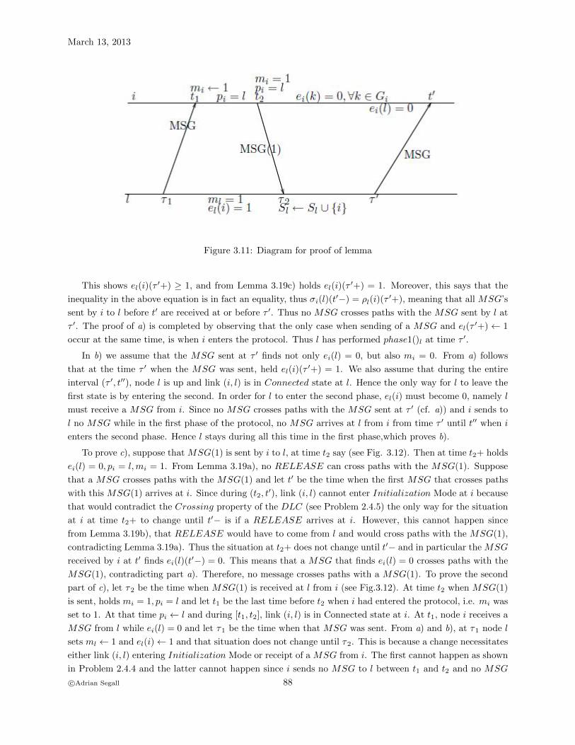
March 13, 2013
Figure 3.11: Diagram for proof of lemma
This shows el(i)(τ′+) ≥ 1, and from Lemma 3.19c) holds el(i)(τ
′+) = 1. Moreover, this says that the
inequality in the above equation is in fact an equality, thus σi(l)(t′−) = ρl(i)(τ
′+), meaning that all MSG’s
sent by i to l before t′ are received at or before τ ′. Thus no MSG crosses paths with the MSG sent by l at
τ ′. The proof of a) is completed by observing that the only case when sending of a MSG and el(τ′+)← 1
occur at the same time, is when i enters the protocol. Thus l has performed phase1()l at time τ ′.
In b) we assume that the MSG sent at τ ′ finds not only ei(l) = 0, but also mi = 0. From a) follows
that at the time τ ′ when the MSG was sent, held el(i)(τ′+) = 1. We also assume that during the entire
interval (τ ′, t′′), node l is up and link (i, l) is in Connected state at l. Hence the only way for l to leave the
first state is by entering the second. In order for l to enter the second phase, el(i) must become 0, namely l
must receive a MSG from i. Since no MSG crosses paths with the MSG sent at τ ′ (cf. a)) and i sends to
l no MSG while in the first phase of the protocol, no MSG arrives at l from i from time τ ′ until t′′ when i
enters the second phase. Hence l stays during all this time in the first phase,which proves b).
To prove c), suppose that MSG(1) is sent by i to l, at time t2 say (see Fig. 3.12). Then at time t2+ holds
ei(l) = 0, pi = l,mi = 1. From Lemma 3.19a), no RELEASE can cross paths with the MSG(1). Suppose
that a MSG crosses paths with the MSG(1) and let t′ be the time when the first MSG that crosses paths
with this MSG(1) arrives at i. Since during (t2, t′), link (i, l) cannot enter Initialization Mode at i because
that would contradict the Crossing property of the DLC (see Problem 2.4.5) the only way for the situation
at i at time t2+ to change until t′− is if a RELEASE arrives at i. However, this cannot happen since
from Lemma 3.19b), that RELEASE would have to come from l and would cross paths with the MSG(1),
contradicting Lemma 3.19a). Thus the situation at t2+ does not change until t′− and in particular the MSG
received by i at t′ finds ei(l)(t′−) = 0. This means that a MSG that finds ei(l) = 0 crosses paths with the
MSG(1), contradicting part a). Therefore, no message crosses paths with a MSG(1). To prove the second
part of c), let τ2 be the time when MSG(1) is received at l from i (see Fig.3.12). At time t2 when MSG(1)
is sent, holds mi = 1, pi = l and let t1 be the last time before t2 when i had entered the protocol, i.e. mi was
set to 1. At that time pi ← l and during [t1, t2], link (i, l) is in Connected state at i. At t1, node i receives a
MSG from l while ei(l) = 0 and let τ1 be the time when that MSG was sent. From a) and b), at τ1 node l
sets ml ← 1 and el(i)← 1 and that situation does not change until τ2. This is because a change necessitates
either link (i, l) entering Initialization Mode or receipt of a MSG from i. The first cannot happen as shown
in Problem 2.4.4 and the latter cannot happen since i sends no MSG to l between t1 and t2 and no MSG
c©Adrian Segall 88

Sec. 3.6
can cross the MSG sent by l at τ1 because of a). Therefore at time τ2− holds ml = 1, el(i) = 1 and i is
included in Sl in <D9>, hence c).
Figure 3.12: Diagram for proof of lemma
Next we prove d). Suppose that node i receives at time t′ a MSG from l = pi while mi = 1, sent by l at
time τ ′. We distinguish between two cases: ei(l)(t′−) = 0 and ei(l)(t
′−) = −1. In the first case, note that
ei(pi) can be 0 while node i is in the protocol, i.e. if mi = 1, only if i is in the second phase of the protocol,
and let t2 be the time when i had entered that phase. (see Fig. 3.11). Let t1 be the last time before t′ when
i has entered the protocol, i.e. has set mi ← 1 and pi ← l. At time t2 node i has sent MSG(1) to l and
during [t1, t′], link (l, i) is in Connected state at i and holds mi = 1. Let τ1 be the time when l has sent the
MSG received by i at t1. From Problem 2.4.6, link (l, i) is in Connected state at l during [τ1, τ′]. During
[t1, t′], node i sends to l only the MSG(1) at t2 and from a), no message crosses paths with the MSG that
arrives at t1, thus the only message that can arrive at l from i during [τ1, τ′] is the MSG(1) sent by i at t2.
Since at τ1+ holds el(i) = 1 and from a), at time τ ′− holds el(i) = 0, some message must arrive on [τ1, τ′]
at l from i, thus the MSG(1) indeed arrives at l, at time τ2 say. By c), at that time holds ml = 1 and i is
included in Sl. From a), at time τ ′− holds ml = 0, and link (i, l) is in Connected state at l between τ2 and
τ ′, so that l receives at least one RELEASE during this period. When the first such RELEASE arrives at
l, it finds ml = 1 and i ∈ Sl, so l sends a RELEASE to i. From Problem 2.4.7, the latter does not get lost
on the link and arrives at i before t′, contradicting the fact that mi = 1 during [t2, t′].
The second case is ei(l)(t′−) = −1. As in the proof of a), ρi(l)(t
′−) = σl(i)(τ′−) and σi(l)(t
′−) ≥ρl(i)(τ
′−). Therefore,
−1 = ei(l)(t′−) = σi(l)(t
′−)− ρi(l)(t′−) ≥ ρl(i)(τ ′−)− σl(i)(τ′−) = −el(i)(τ ′−).
Due to the fact that e can take only values 0 or ±1, this implies el(i)(τ′−) = 1. But this is a contradiction
since in the algorithm, node l never sends a MSG to i at some time τ ′ if el(i)(τ′−) = 1. qed
The statements of Theorem 3.18 are proved now in Lemma 3.21.
Definition: A message is said to be outstanding on a link (i, j) towards j if it had been sent by i, but
has not arrived yet at j. Note that an outstanding message may never arrive at j, due to the latter entering
Initialization mode for that link before the message arrives.
Lemma 3.21
c©Adrian Segall 89
March 13, 2013
a) At any time when mi = 1 and pi = l, if i ∈ Gl, then either ml = 1 or there is a RELEASE outstanding
on link (l, i) towards i ( the condition i ∈ Gl says that l is operational and link (i, l) is in Connected state.)
If ml = 1, then i and l belong to the same segment.
b) At any time, links (i, pi), pi 6= nil such that mi = 1, i ∈ Gpi and there is no outstanding RELEASE on
link (pi, i) traveling towards i, form a forest of disjoint directed trees. All nodes i in a given tree belong to
the same segment.
c) Each tree referred to in b) is rooted at a node i such that mi = 1 and one of the following holds:
(i) pi = nil
(ii) pi 6= nil and i 6∈ Gpi
(iii) pi 6= nil and i ∈ Gpiand there is a RELEASE outstanding on (pi, i) towards i.
The initiator s of a segment is the root of a tree as long as ms = 1. Moreover, nodes in a given tree enter
the second phase in order from leaves to root. No node can enter a tree whose root is of the type (iii) above.
d) Every node can enter a given tree segment??? at most once.5
e) At the time when a node enters the protocol, it sends a MSG to all neighbors, except to pi. When this
MSG arrives at a neighbor, then either that neighbor enters the protocol, or it is in the protocol already.
f) Suppose that there are a finite number of topological changes. A finite time after those changes stop, all
nodes i ∈ V will have mi = 0 and there are no MSG’s in E and this situation does not change (where (V,E)
is the final network).
g) An information message sent by a node i after the final mi ← 0, can be received by a neighbor l only after
the final ml ← 1.
Proof: Suppose that at time t holds mi = 1 and pi = l. At t1, the last time before t when i had set pi ← l, it
had received from l a MSG while mi was 0 (see Fig. 3.11). At the time τ1 when that MSG was sent, node
l had entered the protocol and had set ml ← 1 and el(i)← 1 ( Lemma 3.20a),b). Moreover, link (i, l) is in
Connected state at i during the entire interval [t1, t], so that the Crossing property of DLC shows that link
(l, i) could not have entered Initialization Mode at l and returned to Connected during [τ1, t]. Therefore,
if at time t holds i ∈ Gl, i.e. (l, i) is in Connected state at l, then it is so during the entire interval [τ1, t]. We
shall show that either ml, that had value 1 at τ1+, does not change until time t or there is a RELEASE
outstanding at time t on the link (l, i) from l to i. Since ml can change only if l receives a RELEASE
and the later can be received only if all el(k) are 0 (Lemma 3.19b)), the variable ml stays 1 at least until l
receives a MSG from i that resets el(i) to 0. From Lemma 3.20a), that MSG cannot cross paths with the
MSG sent at τ1, thus it can be sent only after t1 and hence it is a MSG(1). From Lemma 3.20c), it also
causes inclusion of i into Sl. Therefore, if ml does change before t, it does so at a time when i ∈ Sl, so l
sends RELEASE to i. That RELEASE is still outstanding at time t, because if it arrived beforehand, it
would have set mi ← 0, contradicting the fact that mi = 1 on the entire interval (t1, t]. Hence the first part
of a). If ml = 1 at time t, then l has entered its current segment at τ1 and has sent to i a MSG of that
segment. Thus at time t1, node i enters the same segment.
To prove the first part of b), we only have to show that if at time t, a node i enters the protocol, i.e.
sets mi ← 1, and selects l as pi, it does not close a loop with the property that for all its links (n, pn) holds
5Example when a node can enter a given segment ???? twice (link comes up).
c©Adrian Segall 90

Sec. 3.6
mn = 1, no RELEASE is outstanding from pn to n and n ∈ Gpn . But at time t− holds mi = 0, so that by
a), there is no node j with mj = 1, pj = i, j ∈ Gi and no RELEASE outstanding from i to j, so no such
loop can be closed. The second part of b) follows from the second part of a).
A root of a tree referred to in b) is a node i such that mi = 1 and either pi = nil or (i, pi) does not satisfy
one of the conditions in b). In case (i) holds pi = nil, while in cases (ii) and (iii) one of the conditions in b)
are not satisfied. If i is the initiator of a segment, then since pi = nil as long as mi = 1, the initiator of a
segment is the root of the tree as long as mi = 1. Since from Lemma 3.20b), as long as node i is in the first
phase and i ∈ Gpi , its preferred neighbor pi is also in the first phase, no node can enter the second phase
before all its sons in the tree do so. Therefore the root of the tree is the last in the tree to enter the second
phase. In fact the root exits the protocol instead of entering the second phase (see <G5>), so that the root
can exit the protocol only after all nodes in the tree enter the second phase.
The above only shows that the root of a tree does not exit the protocol before all nodes already in the
tree enter the second phase. It remains to show that no node enters a tree whose root is of type (iii), namely
such that (s, ps) is in Connected state at both ends and there is a RELEASE outstanding towards s on
(ps, s). Suppose that this is not the case and let node i be the first node to enter such a tree, i.e. perform
phase1()i, at a time t say. Let l be the node from which i receives a MSG at time t. Node l has entered
the tree before the RELEASE has been sent
the time when s had exited it and on the other hand, node l is at time t still in the first phase (Lemma
3.20b)). This means that s exits the segment while l is still in the first phase, contradicting the statements
in the previous paragraph. in the tree is in the first phase.
To prove d), suppose a node i is the first to enter the same segment for the second time, at time t. This
means that prior to t, node i had been in that segment and had exited it. From c), this means that the root
of the tree had exited the segment before time t. This contradicts the other part of c), that states that no
node can enter a segment after the time when the root had exited it.
To prove e), consider first a leaf i of a tree corresponding to a given segment. When it enters the segment,
it sends a MSG to all neighbors k except pi and sets ei(k)← 1. When the MSG arrives at a neighbor k, it
finds mk = 1, since otherwise k would select i as its preferred neighbor and i would not be a leaf. Note that
k may be in the same segment as i or in a different one and that by Lemma 3.20d), at the time when the
MSG arrives at k, the variable ek(i) cannot be −1. If at that time, ek(i) = 0, then k sends a MSG back to
i ( see phase3()). If ek(i) = 1, then k had previously sent a MSG to i, that crosses paths with the one sent
by i to k. In both cases, when the MSG sent by k is received at i, it sets ei(k) ← 0. When this happens
for all neighbors except pi, node i enters the second phase and sends MSG(1) to its preferred neighbor.
This process continues downtree until all nodes enter the second phase. By Lemma 3.20c), when a node i
enters the second phase, its list Si contains exactly the sons of i in the tree, i.e. the neighbors that had
sent MSG(1) to i. When the segment initiator is supposed to enter the second phase, it exits the segment
instead (see phase4()) and sends RELEASE to all neighbors in Ss, i.e. to all sons in the tree. Similarly,
when a node i receives RELEASE, it exits the segment and sends RELEASE to its sons. 6 Consequently,
all nodes in the tree eventually set mi ← 0 and no more messages of the segment can subsequently be sent
or received. qed
?????? Partial PIF’s
In various situations, it may be important to allow certain nodes to refuse to enter a PIF protocol. This
may be the situation if for example, the nodes are temporarily busy in another protocol. The refusal may
be temporary, so that receipt of a message at a subsequent time may cause the same node to enter the PIF.
Obviously, when nodes are allowed to temporarily refuse entrance in the protocol, one cannot expect the
6Show that the above protocol with PI3 instead of PIF3 does not work.
c©Adrian Segall 91

March 13, 2013
information to reach all nodes in the network, but we shall show that in this situation
c©Adrian Segall 92

Sec. 3.7
3.7 Generalized PIF (GPIF)
In this section we generalize the PIF protocol introduced in Section 3.3.2. Many protocols will prove to be
special cases of the Generalized PIF .
In the Generalized PIF it is required that every node i in the network receives at least one message
MSG. As in PIF , in the first stage of the Generalized PIF, every node i enters the protocol when it receives
the first MSG; if l is the neighbor from which that message was received, i sets at that time pi ← l. In this
way a spanning tree rooted at s is defined by the collection {(i, pi),∀i ∈ V }. However we do not necessarily
require that upon entering the protocol, every node i will send messages to all k ∈ Gi − {pi}.Before introducing the generalization for the second stage, it will be useful to rename the message sent
by a node i in phase2()i of PIF to its preferred neighbor. This message will be called here ECHO. Also,
for a node i, we introduce the notation Si as the set of sons of i in the tree constructed in the first phase,
i.e. Si = {k : pk = i}. Observe that node i does not know the set Si.
Now recall that the purpose of PIF was to deliver to the initiator s confirmation that the information
has reached all nodes in the network. Observe that in principle, in order to achieve this goal, it is not
necessary that nodes wait to receive messages from all Gi − {pi} before performing phase2()i. Receipt of
ECHO messages from all sons k ∈ Si would suffice. The difficulty in implementing this change is that the
set Si is not known to i. The solution in PIF was to wait for MSG or ECHO from all k ∈ Gi−{pi}. Since
the latter set includes Si, we are sure that when phase2()i is performed, ECHO messages have indeed been
received from all neighbors in Si. In doing so we have achieved the additional property that when phase2()i
is performed, there are and will be no messages traveling towards i, so that when the Protocol initiator s
completes the protocol, i.e. performs phase2()s, the entire network is and will be free of messages. The
above properties will also be preserved in the Generalized version.
A predicate at node i is a boolean function on the state of node i. Following [CL85] , in a given protocol,
we say that a predicate at i is stable after a time ti ≤ ∞ if it is false before ti, becomes true at time ti
and stays true forever afterwards. For a neighbor l ∈ Si, we define Ni(l) as a predicate that is true after
ECHO is received from l and false beforehand. Obviously, Ni(l) is a stable predicate. A predicate Yi
at i will be said to be confirming for a given protocol, if it satisfies the following properties:
a) stability: Yi is stable at i in the protocol and becomes true at a finite time ti <∞.
b) detectability: node i can detect if and when the stable predicate (Yi and Ni(l),∀l ∈ Si) becomes true ,
without the knowledge of Si.
c) quiescence: no message travels on a link (i, k) after the later of the times when in the given protocol
(Yi and Ni(l),∀l ∈ Si) becomes true and (Yk and Nk(l),∀l ∈ Sk) becomes true .
For example, the predicate Yi =( node i has received a MSG from all k ∈ Gi − Si − {pi}) is confirming
for PIF . The trivial predicate Yi ≡ true is not confirming for any reasonable protocol, since it does not
satisfy at least detectability.
Definition: A protocol is said to be a Generalized PIF on a network (V,E) if every node i ∈ V receives
at least one message MSG and if the protocol consists of two phases:
i) In the first phase, denoted by phase1()i, every node i enters the protocol when it receives the first message
MSG; if l is the neighbor from which this message is received, node i sets pi ← l.
ii) A node i performs its part of the second phase, denoted by phase2()i, when and if
(Yi and Ni(l),∀l ∈ Si) becomes true , where Yi is a confirming predicate for the protocol. At that time
it sends an ECHO message to pi.
c©Adrian Segall 93

March 13, 2013
In particular, PIF is a generalized PIF with the confirming predicate Yi = (node i has received a MSG
from all k ∈ Gi − Si − {pi}).Protocol GPIF
Messages
MSG(info) - message carrying the information infoECHO -message serving as confirmation
Variables
Gi - set of neighbors of imi - shows if node i has already entered the protocol (values 0,1);pi - preferred neighbor, i.e. neighbor from which MSG was received first.Ni(l) = true after i has received ECHO from l,= false otherwise ( for all l ∈ Gi )
Initialization
if a node i receives a MSG, then
- just before receiving the first MSG, holds mi = 0- after receiving the first MSG, node i discards and disregards messages not sent in the present instanceof the protocol
Algorithm for node i
A1 receive MSG(info) from l ∈ Gi ∪ {nil}A2 { if (mi = 0) {A3 initalize();A4 phase1();
}}
B1 receive ECHO from l ∈ GiB2 { Ni(l)← true ;
}C1 (Yi and Ni(l
′),∀l′ ∈ Si) becomes trueC2 { phase2();
}D1 phase1()D2 { mi ← 1;D3 pi ← l;D4 accept(info);
}E1 phase2()E2 { send ECHO to pi
}F1 initialize()F2 { for (k ∈ Gi − {pi}) Ni(k)← false ;
}
Theorem 3.22 ( Generalized PIF ) Suppose that in a Generalized PIF Protocol node s receives START .
Then:
a) all connected nodes i will perform the event phase1()i in finite time and exactly once; after this happens,
the links {(i, pi),∀i ∈ V } will form a directed tree rooted at s; in addition, for all i holds t(phase1()i) >
t(phase1()pi).
b) node s and all connected nodes i will perform phase2()i in finite time and exactly once; moreover t(phase1()i) ≤t(phase2()i) < t(phase2()pi); also, when node s performs phase2()s, all Yi’s hold, all nodes will have com-
pleted the algorithm, i.e. performed phase2() and there are no messages traveling in the network.
Proof: In the definition of the Generalized PIF it is assumed that every node i enters the protocol. Node
i selects the neighbor from which it receives the message that causes i to enter the protocol as pi. Since the
latter can send a message only after it enters itself the protocol, it has previously performed phase1()pi.
c©Adrian Segall 94

Sec. 3.7
This also implies that {(i, pi), ∀i ∈ V } is a tree rooted at s. Hence a). To prove b), let k be a leaf of the tree
referred to in a), i.e. 6 ∃l such that pl = k. Since Sk = Φ, the condition for phase2()k will become true
when Yk becomes true . At that time node k will send ECHO to pk. The same will be true for all leaves.
When those messages arrive, a node i in the last-but-one level in the tree will have (Ni(l),∀l ∈ Si) = true .
Therefore, when its Yi will become true ,it will be able to perform phase2()i. The procedure will continue
downtree all the way to node s. Since s performs phase2() last in the network, and Yi has the quiescence
property, at time t(phase2()s) there are no messages in the network, completing the proof. qed
3.7.1 Distributed Snapshots (DS)
In a given protocol P , consider a collection of instances {ti,∀i ∈ V } such that every message of P received
by a node k from a neighbor i before tk was sent by i before ti. The state of node i in P at time ti is
denoted by si. The state s(i,k) of the link (i, k) corresponding to this collection of times is defined as the
sequence of messages sent by i in P on link (i, k) before ti and received by k after tk. A Distributed Snapshot
[CL85], [Gaf86] is the collection of node states si and link states s(i,k) corresponding to a collection of times
ti with the property mentioned above. Distributed Snapshots are useful in several classes of problems. For
example, it can be shown [CL85] that if protocol P is in a deadlock situation during the snapshot, it is in
this situation at any time later. Similarly, if the snapshot discovers termination of P . Hence snapshots are
useful in discovering stable network states, like deadlock or termination. A PI1 protocol can be used to
determine a Distributed Snapshot for an arbitrary protocol P as follows [CL85]. The Distributed Snapshot
protocol, denoted by DS1, is given below.Protocol DS1
Algorithm for node i
A1 receives MSG from l ∈ Gi ∪ {nil}A2 { if (mi = 0) phase1();A3 else s(l,i) ← sequence of messages of P received on (l, i) since ti;
}B1 phase1()B2 { mi ← 1;B3 pi ← l;B4 ti ← current time;B5 si ← current state of i;B6 s(pi,i) ← empty sequence;B7 for (k ∈ Gi) send MSG to k;
}
Theorem 3.23 (DS1) Protocol DS1 generates a Distributed Snapshot.
Proof: As in Theorem 3.1, let
t(sendk(i)) = time when k sends MSG to neighbor i
t(rcvk(i)) = time when k receives MSG from neighbor i.
Then for any two neighbors i and k, holds ti = t(sendi(k)) and tk ≤ t(rcvk(i)). The FIFO property implies
that every message of the underlying protocol P received by k from i before t(rcvk(i)) was sent before
t(sendi(k)) and therefore every message received by k from i before tk was sent before ti. Moreover, the
state of the link (i, k) is registered in <A3> as the sequence of P messages received by k on (i, k) between
tk and t(rcvk(i)). This is exactly the sequence of P messages sent by i on (i, k) before t(sendi(k)) = ti and
not received by k until tk. qed
A combination of PI1 and PIF1 can be used to allow a node s to collect the information of the Distributed
Snapshot. This is Protocol DS2.
c©Adrian Segall 95

March 13, 2013
Protocol DS2
Algorithm for node i
A1 receives MSG or MSG′ from l ∈ Gi ∪ {nil}A2 { if (mi = 0) {A3 initialize();A4 phase1();
}A5 else {A6 if (received MSG) ei(l)← ei(l)− 1;A7 else s(l,i) ← sequence of messages of P received on (l, i) since ti;
}A8 if (ei(l
′) = 0 ∀l′ ∈ Gi − {pi}) phase2();}
B1 phase1()B2 { mi ← 1;B3 pi ← l;B4 ti ← current time;B5 si ← current state of i;B6 s(pi,i) ← empty sequence;B7 for (k ∈ Gi − {pi}) {B8 send MSG to k;B9 ei(l)← ei(l) + 1;
}B10 send MSG′ to pi;
}C1 phase2()C2 { put (si, s(k,i) ∀k ∈ Gi and all s’s received in MSG’s ) into MSG;C3 send MSG to pi;
}D1 initialize()D2 { for (k ∈ Gi) ei(k)← 0;
}Except for lines <C1>-<C3>, Protocol DS2 is the same as DS1 where the message sent by i to pi in
<C3> is renamed MSG′. Therefore DS2 generates a Distributed Snapshot. Superimposed on that, the
collection of messages MSG defines a PIF , where the MSG’s sent to preferred neighbors collect the states
of the descendants in the tree. Consequently, when s performs phase2()s it has the Distributed Snapshot
information from the entire network. We have therefore proved:
Theorem 3.24 (DS2) Protocol DS2 defines a Distributed Snapshot. Also, node s will perform phase2()s
in finite time and at that time it has the information of the Distributed Snapshot states of the entire network.
3.7.2 The Echo Protocol
The Echo Protocol of [Cha78],[Cha82] accomplishes the same task as PIF , with twice as many messages.
We bring it here for completeness and because it will be used in later protocols. The first phase is a PI2
protocol. When a node i receives a MSG while mi = 1, it returns on the same link an ECHO′ message.
When a node i receives ECHO or ECHO′ messages from all neighbors, it performs phase2()i and sends an
ECHO message to pi. Therefore the Echo Protocol is a Generalized PIF , with a PI2 as its first phase and
with Yi = (ECHO′ received from all k ∈ Gi−Si−{pi}). In fact it turns out that the actions in response to
receipt of ECHO and ECHO′ are the same, so we shall distinguish between them only in the explanations
and the proofs. In the code, both types will be called ECHO.
c©Adrian Segall 96

Sec. 3.7
Protocol ECHO
Messages
MSG(info) - message containing the information info to be distributed ( in [Cha78] , this is called anexplorer message )ECHO - echo message to MSG, as well as a message serving for confirmationSTART - message received from the outside world
Variables
Gi - set of neighbors of imi - shows if node i has already entered the protocol (values 0,1)pi - neighbor from which MSG was received firstei(l) = number of MSG’s sent − number of ECHO’s received on link (i, l) ( ∀l ∈ Gi)
Initialization
if a node i receives a MSG, then
- just before receiving the first MSG, holds mi = 0.- after receiving the first MSG, node i discards and disregards messages not sent in the present instanceof the protocol
Note: By definition, a condition on an empty set is always true. For example, in <B3> below, ifGi − {pi} = ∅, then the condition holds and i should perform phase2().
Algorithm for node i
A1 receives MSG(info) from l ∈ Gi ∪ {nil}A2 { if (mi = 0) {A3 initialize();A4 phase1();A5 if (Gi = pi) phase2();
}A6 else send ECHO to l;
}B1 receives ECHO from l ∈ GiB2 { ei(l)← ei(l)− 1;B3 if (ei(k) = 0 ∀k ∈ Gi − {pi}) phase2();
}C1 phase1() /* similar to PI2 */C2 { mi ← 1;C3 pi ← l;C4 accept(info);C5 for (k ∈ Gi − {pi}){C6 send MSG(info) to k;C7 ei(k)← ei(k) + 1;
}}
D1 phase2()D2 { send ECHO to pi;
}E1 initialize()E2 { for (k ∈ Gi) ei(k)← 0;
}In the proof we shall refer to the ECHO messages sent in <A6> as ECHO′ and to the ones sent in
<D2> as ECHO.
Lemma 3.25 (ECHO) The Echo Protocol is a Generalized PIF with a PI2 as its first phase and with
Yi = (ei(l′) = 0,∀l′ ∈ Gi − Si − {pi}).
Proof: The actions in phase1()i are identical to those of PI2, with the addition that ei(l) is set to 1
when MSG is sent by i to l. Messages MSG are sent by a node i only in phase1()i to all k ∈ Gi − {pi}.When a MSG arrives to such a neighbor k, it either finds it with mk = 1, in which case k ∈ Gi − Si − {pi}or with mk = 0, in which case k ∈ Si. In the first case, k sends an ECHO′ to i in <A6> and afterwards
c©Adrian Segall 97

March 13, 2013
sends no messages to i. The receipt of this message at i sets ei(k)← 0. Since afterwards no ECHO arrives
at i from k and no MSG is sent by i to k, the event ei(k) = 0 is stable and therefore Yi is stable. After a
node k ∈ Si sends ECHO to i in phase2()k, it does nothing and that ECHO sets Ni(k)← true when it
arrives. Therefore, for k ∈ Si, after ei(k) is set to 0, no message arrives to i from k. Since after t(phase1()i)
no message arrives at i from pi and after the time when ei(l) ← 0 for any l ∈ Gi − Si − {pi}, no message
arrives at i from l, Yi satisfies the quiescence property. Obviously it satisfies the detectability property, since
(Yi and Ni(l),∀l ∈ Si) ≡ (ei(l) = 0,∀l ∈ Gi − {pi}). qed
This completes the proof of the Lemma and therefore of the following Theorem.
Theorem 3.26 (ECHO) Suppose node s receives START. Then:
a) all connected nodes i will perform the event phase1()i in finite time and exactly once; after this happens,
the links {(i, pi) ∀i ∈ V } will form a directed tree rooted at s; in addition, for all i holds t(phase1()pi) >
t(phase1()i). Moreover, the propagation of information is the fastest possible.
Note: some nodes may perform phase2() before all nodes have performed phase1() )
b) node s and all connected nodes i will perform phase2()i in finite time and exactly once; moreover t(phase1()i) ≤t(phase2()i) < t(phase2()pi
) also, when node s performs phase2()s , all connected nodes will have completed
the algorithm, i.e. performed phase2() and there are no messages traveling in the network.
c) on all links 6= (i, pi), exactly one MSG and one ECHO travels on each link in each direction; on all links
of the type (i, pi), exactly one MSG travels from pi to i and one ECHO travels in the other direction7.
3.7.3 Termination Detection for Diffusing Computations (TDDC)
The problem is the following [DS80]. A node s starts the protocol by sending some messages MSG to
some of its neighbors. A node i enters the protocol when it receives the first message MSG. Afterwards
it may perform some computations that may require it to send some messages MSG, a finite number of
them, to neighbors. Eventually, a node is in a situation when it sends no more messages MSG of the
computation. We say then that the node has terminated the computation. A node i that receives a MSG
but has no computation to perform and hence sends no messages MSG is considered as if it had terminated
the computation. The problem is to superimpose on the above a signalling scheme that will allow the source
s to know that all nodes have indeed terminated their computations and will receive no more messages.
The signalling protocol proposed in [DS80] is the following: whenever a node i receives the first MSG,
from a neighbor l say, it denotes pi ← l and enters the protocol. Subsequently, whenever it receives some
MSG, from a neighbor k say, it returns to k a signalling message ECHO. It does that whether it is still
performing the computation or it had already terminated it. Recall that if it has no computation to perform,
node i is considered to have terminated the computation, so that it returns an ECHO even in response to
the first MSG. After having terminated the computation, node i waits until it receives an ECHO for every
MSG it has sent and then it sends an ECHO message to pi. The latter is the response to the first received
MSG. When the initiator s terminates its computation and receives an ECHO for every MSG sent, it
knows that all nodes that have started the computation have terminated it and there are no messages in the
network. Observe that this protocol does not guarantee that all nodes that have a computation to perform
indeed enter the protocol. The solution to this is given in Problem 3.7.2 and in the second version of TDDC,
presented in the next section.
7Communication complexity ???
Time complexity ???
c©Adrian Segall 98
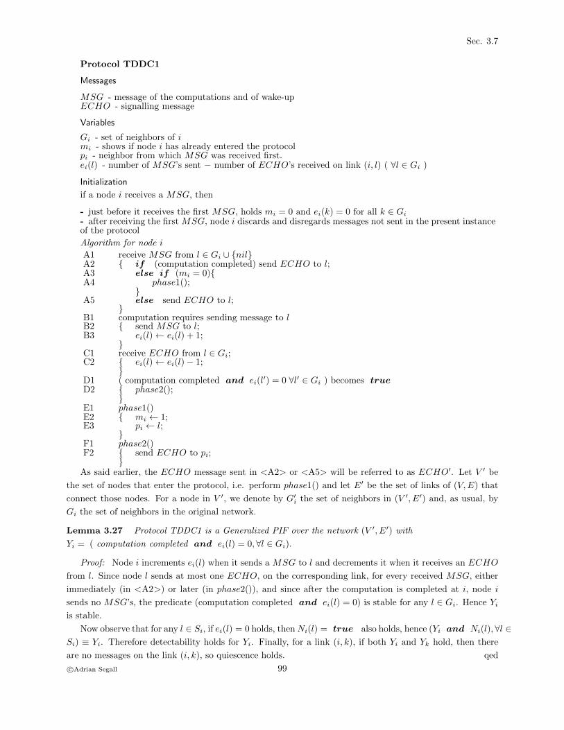
Sec. 3.7
Protocol TDDC1
Messages
MSG - message of the computations and of wake-upECHO - signalling message
Variables
Gi - set of neighbors of imi - shows if node i has already entered the protocolpi - neighbor from which MSG was received first.ei(l) - number of MSG’s sent − number of ECHO’s received on link (i, l) ( ∀l ∈ Gi )
Initialization
if a node i receives a MSG, then
- just before it receives the first MSG, holds mi = 0 and ei(k) = 0 for all k ∈ Gi
- after receiving the first MSG, node i discards and disregards messages not sent in the present instanceof the protocol
Algorithm for node i
A1 receive MSG from l ∈ Gi ∪ {nil}A2 { if (computation completed) send ECHO to l;A3 else if (mi = 0){A4 phase1();
}A5 else send ECHO to l;
}B1 computation requires sending message to lB2 { send MSG to l;B3 ei(l)← ei(l) + 1;
}C1 receive ECHO from l ∈ Gi;C2 { ei(l)← ei(l)− 1;
}D1 ( computation completed and ei(l
′) = 0 ∀l′ ∈ Gi ) becomes trueD2 { phase2();
}E1 phase1()E2 { mi ← 1;E3 pi ← l;
}F1 phase2()F2 { send ECHO to pi;
}As said earlier, the ECHO message sent in <A2> or <A5> will be referred to as ECHO′. Let V ′ be
the set of nodes that enter the protocol, i.e. perform phase1() and let E′ be the set of links of (V,E) that
connect those nodes. For a node in V ′, we denote by G′i the set of neighbors in (V ′, E′) and, as usual, by
Gi the set of neighbors in the original network.
Lemma 3.27 Protocol TDDC1 is a Generalized PIF over the network (V ′, E′) with
Yi = ( computation completed and ei(l) = 0,∀l ∈ Gi).
Proof: Node i increments ei(l) when it sends a MSG to l and decrements it when it receives an ECHO
from l. Since node l sends at most one ECHO, on the corresponding link, for every received MSG, either
immediately (in <A2>) or later (in phase2()), and since after the computation is completed at i, node i
sends no MSG’s, the predicate (computation completed and ei(l) = 0) is stable for any l ∈ Gi. Hence Yi
is stable.
Now observe that for any l ∈ Si, if ei(l) = 0 holds, thenNi(l) = true also holds, hence (Yi and Ni(l),∀l ∈Si) ≡ Yi. Therefore detectability holds for Yi. Finally, for a link (i, k), if both Yi and Yk hold, then there
are no messages on the link (i, k), so quiescence holds. qed
c©Adrian Segall 99

March 13, 2013
This completes the proof of the Lemma and therefore of the following Theorem.
Theorem 3.28 (TDDC1) Suppose node s receives START. Then node s and all connected nodes i that enter
the protocol will perform phase2()i in finite time and exactly once; moreover t(phase1()i) ≤ t(phase2()i) <
t(phase2()pi); also, when node s performs phase2()s, all nodes that have entered the protocol will have
completed the algorithm, i.e. performed phase2() and there are no messages traveling in the network.
3.7.4 Termination Detection for Diffusing Computations - Version 2
Version 1 is not appropriate if there are one or more nodes i that need to perform a computation, but there
is no neighbor of i whose computation requires it to send a message to i. This is because such a node i will
never enter the protocol. The present version will work for this case. As seen below, the present version is
also more economical in terms of messages in most situations.
In order to allow all nodes to enter the protocol, the first phase in this version will be a PI2 protocol with
wake-up messages, which we call MSG. After entering the protocol, a node starts its computation and sends
computation messages, called COMP , to neighbors as required. No reply messages to COMP are needed
in this version. When it completes its computation, a node i sends a completion message, called ECHO,
to each of its neighbors, except to pi. Subsequently, if it receives some (late) message MSG, it responds
with an ECHO. Finally, when it had received a ECHO message from all neighbors and had completed
the computation, it sends a ECHO message to pi. Receipt of an ECHO message from all neighbors at s
indicates completion of the protocol in the entire network.
The present version is more economical in terms of messages if there are many computation messages to
be sent, since in the previous version, an ECHO was sent for each of these messages.
Note that the present version is exactly the Echo Protocol, except that the transmission of the ECHO
messages is postponed until completion of the computation. Hence,
Lemma 3.29 (TDDC2) The TDDC2 Protocol is a Generalized PIF with
Yi = (computation completed and ei(l′) = 0, ∀l′ ∈ Gi − Si − {pi}) and with the first phase corresponding
to a PI2 protocol.
3.7.5 Synchronizers
In a synchronous protocol, messages are allowed to be sent only at integer times and the delay of each
message is at most one time unit. In an asynchronous network, for each node i, consider a sequence of
instances {ti(0), ti(1), ti(2), . . . }. These sequences of instances define a synchronizer [Awe85a] for a given
execution of a protocol P if:
a) messages of P can be sent by i only at times {ti(n), n ≥ 0}.
b) messages of P sent by i to neighbor k at time ti(n) arrive at k before tk(n+ 1).
c) messages of P sent by i to neighbor k at time ti(n) arrive at k after tk(n).
Note that the definition of a synchronizer in [Awe85a] omits requirement c). The latter is however re-
quired if the asynchronous protocol is to behave as a synchronous one. The simplest synchronizer, called
synchronizer α in [Awe85a] works as follows. The initial times ti(0) can be set by nodes by a PI1 or
PI2 protocol. Whenever a node i enters the PI, it sets the tick ti(0). In general, when a node i com-
pletes sending to k the messages corresponding to tick ti(n), it sends to k a message SY NCH(n). The
time incorrect??,safe,ack, [LT87], [SS91] ti(n + 1) is defined as the time when i has received mes-
sages SY NCH(n) from all its neighbors. With this protocol, conditions a) and b) above are satisfied. If
c©Adrian Segall 100

Sec. 3.7
Protocol P is such that it ensures that no P message sent by a node i at tick ti(n) arrives at k before tk(n)
for all (i, k), then the instances defined above define a synchronizer for P .
Another synchronizer designed in [Awe85a], called synchronizer β, uses asymptotically (in the size of the
network) less messages, but longer time. This synchronizer needs an initialization phase, where a leader
s is selected in the network and a spanning tree, rooted at s is built. In this protocol it is required that
every node i learns that all messages of Protocol P sent to neighbors in round (n− 1) have arrived, before
being able to participate in the protocol for determining tk(n),∀k. In order to save messages, we exploit
the Confirm property of the DLC that states that every considered acknowledged data packet has been
delivered to the other side. Recall that messages of Protocol P (as well as any messages of levels higher than
the DLC level) are considered as data packets by the DLC. If, when the DLC considers the packet containing
a P message acknowledged, it also informs the local synchronizer algorithm, this information can be used by
the latter to know that the message has indeed arrived to the other side. Eventually a node i will find out
that all P messages sent at tick ti(n − 1) have been delivered. At that time node i is said to be safe with
respect to tick (n− 1).
The rest now is like a PIF on the tree, except that phase (ii) of the PIF is performed first. When leaves
learn that they are safe , they send to their father in the tree a SY NCH(n−1) message. In general, when a
node learns that it is safe and has received SY NCH(n−1) messages from all sons, it sends a SY NCH(n−1)
message to its father. When the leader s receives SY NCH(n− 1) from all its sons, it knows that all nodes
are safe, and triggers broadcast of a SY NCH(n) message over the tree. The time ti(n) is defined as the
time when i receives the SY NCH(n) message. As shown in the Problem 3.7.8, messages sent by i at tick
ti(n) can arrive at a neighbor k between tk(n− 1) and tk(n+ 1). Therefore, in order to have a synchronizer,
we have to require here also that no P message sent by a node i at tick ti(n) arrives at k before tk(n) for
all (i, k). The communication load of this protocol is 0(| V |) per tick, plus the communication load of the
spanning tree construction and of the leader election, as opposed to the simple synchronizer presented above,
whose communication load is O(| E |) per tick.
Problems
Problem 3.7.1 Give examples of various predicates {Yi} and check whether they are confirming.
Problem 3.7.2 Protocol TDDC1 does not ensure that all nodes that have a computation to perform indeed
enter the protocol. Indicate a protocol that solves this problem, based on TDDC1 and other protocols in
this Chapter.
Problem 3.7.3 Write the code for TDDC2.
Problem 3.7.4 Show that with the SY NCH messages sent as in synchronizer α, P messages sent at tick
ti(n) can arrive at a neighbor k only between tk(n− 1) and tk(n+ 1).
Problem 3.7.5 Various protocols in this chapter, and synchronizers for them.
Problem 3.7.6 Suggestion: use two types of SYNCH(n) messages, one before P messages of ti(n) and one
after. Does this work???
Problem 3.7.7 Which of the protocols ECHO,PI, PIF, DS, TDDC, can be made more efficient by using
the Confirm property of the DLC. Write the corresponding codes and prove their correctness.
Problem 3.7.8 Show that with protocol β , messages sent by i at tick ti(n) can arrive at a neighbor k
between tk(n− 1) and tk(n+ 1).
c©Adrian Segall 101
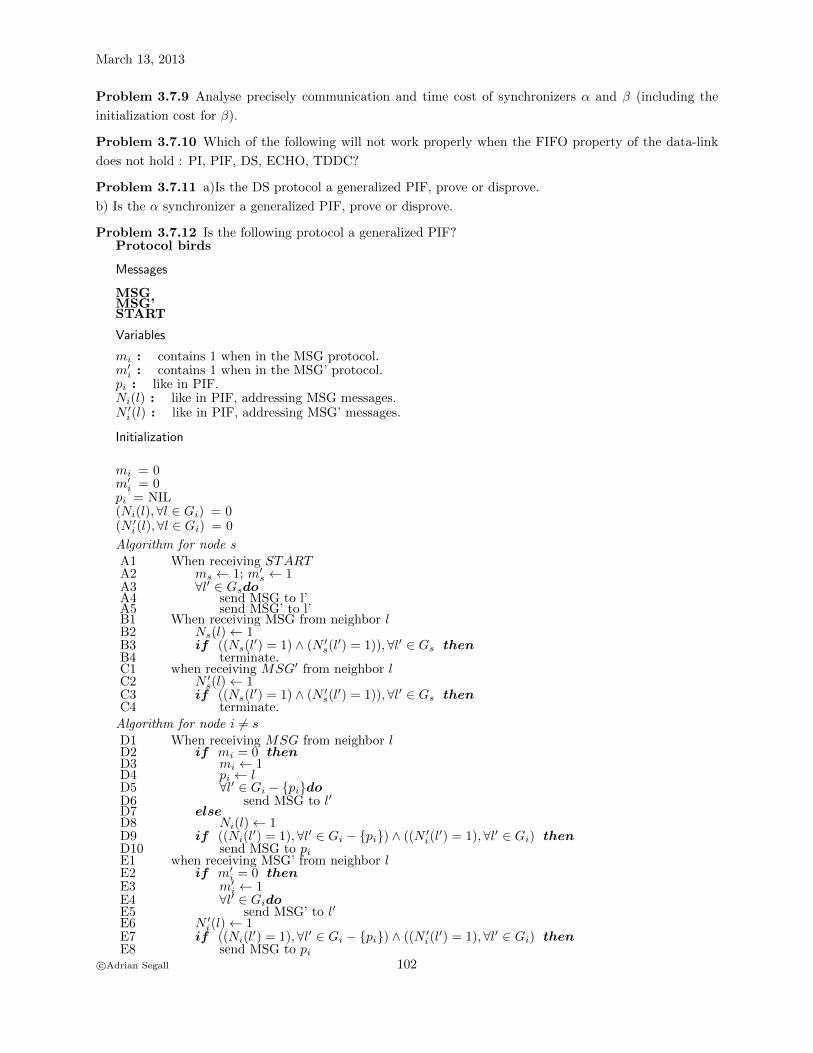
March 13, 2013
Problem 3.7.9 Analyse precisely communication and time cost of synchronizers α and β (including the
initialization cost for β).
Problem 3.7.10 Which of the following will not work properly when the FIFO property of the data-link
does not hold : PI, PIF, DS, ECHO, TDDC?
Problem 3.7.11 a)Is the DS protocol a generalized PIF, prove or disprove.
b) Is the α synchronizer a generalized PIF, prove or disprove.
Problem 3.7.12 Is the following protocol a generalized PIF?Protocol birds
Messages
MSGMSG’START
Variables
mi : contains 1 when in the MSG protocol.m′i : contains 1 when in the MSG’ protocol.pi : like in PIF.Ni(l) : like in PIF, addressing MSG messages.N ′i(l) : like in PIF, addressing MSG’ messages.
Initialization
mi = 0m′i = 0pi = NIL(Ni(l),∀l ∈ Gi) = 0(N ′i(l),∀l ∈ Gi) = 0
Algorithm for node sA1 When receiving STARTA2 ms ← 1; m′s ← 1A3 ∀l′ ∈ GsdoA4 send MSG to l’A5 send MSG’ to l’B1 When receiving MSG from neighbor lB2 Ns(l)← 1B3 if ((Ns(l
′) = 1) ∧ (N ′s(l′) = 1)),∀l′ ∈ Gs then
B4 terminate.C1 when receiving MSG′ from neighbor lC2 N ′s(l)← 1C3 if ((Ns(l
′) = 1) ∧ (N ′s(l′) = 1)),∀l′ ∈ Gs then
C4 terminate.
Algorithm for node i 6= sD1 When receiving MSG from neighbor lD2 if mi = 0 thenD3 mi ← 1D4 pi ← lD5 ∀l′ ∈ Gi − {pi}doD6 send MSG to l′D7 elseD8 Ni(l)← 1D9 if ((Ni(l
′) = 1),∀l′ ∈ Gi − {pi}) ∧ ((N ′i(l′) = 1),∀l′ ∈ Gi) then
D10 send MSG to piE1 when receiving MSG’ from neighbor lE2 if m′i = 0 thenE3 m′i ← 1E4 ∀l′ ∈ GidoE5 send MSG’ to l′E6 N ′i(l)← 1E7 if ((Ni(l
′) = 1),∀l′ ∈ Gi − {pi}) ∧ ((N ′i(l′) = 1),∀l′ ∈ Gi) then
E8 send MSG to pic©Adrian Segall 102

Sec. 3.7
Problem 3.7.13 The protocol of Problem 3.7.12 has been changed as follows: Two nodes in the network
— s and s’ receive asynchronously each a START message. The algorithm of all the nodes except s and s’
has not been changed.Protocol birds1
Algorithm for node sA1 When receiving STARTA2 ms ← 1A3 ∀l′ ∈ GsdoA4 send MSG to l′B1 When receiving MSG from neighbor lB2 Ns(l)← 1B3 if ((Ns(l
′) = 1) ∧ (N ′s(l′) = 1)),∀l′ ∈ Gs then
B4 terminate.C1 when receiving MSG′ from neighbor lC2 if m′s = 0 thenC3 m′s ← 1C4 ∀l′ ∈ GsdoC5 send MSG′ to l′C6 N ′s(l)← 1C7 if ((Ns(l
′) = 1) ∧ (N ′s(l′) = 1)),∀l′ ∈ Gs then
C8 terminate.
Algorithm for node s′
D1 When receiving STARTD2 m′s′ ← 1D3 ∀l′ ∈ Gs′doD4 send MSG’ to l′E1 When receiving MSG from neighbor lE2 if ms′ = 0 thenE3 ms′ ← 1E4 ps′ ← 1E5 ∀l′ ∈ Gs′ − {ps′}doE6 send MSG to l′E7 elseE8 Ns′(l)← 1E9 if ((Ns′(l
′) = 1),∀l′ ∈ Gs′ − {ps′}) ∧ ((N ′s′(l′) = 1),∀l′ ∈ Gs′) then
E10 send MSG to ps′F1 when receiving MSG’ from neighbor lF2 N ′s′(l)← 1F3 if ((Ns′(l
′) = 1),∀l′ ∈ Gs′ − {ps′}) ∧ ((N ′s′(l′) = 1),∀l′ ∈ Gs′) then
F4 send MSG to piIs this a generalized PIF?
c©Adrian Segall 103

March 13, 2013
c©Adrian Segall 104

Chapter 4
CONNECTIVITY TEST
PROTOCOLS
The purpose of this class of DNP’s [Seg83] is to allow each node to learn what nodes are connected to it, i.e.
nodes that are in V .
4.1 Protocol CT1
The idea here is to use protocol PI1 repeatedly, first to inform all nodes that the protocol is in progress
and then for each node to propagate its own identity. Every node (or several nodes) can start the protocol
by receiving START . A node enters the protocol whenever it receives either START or the first control
message from any of its neighbors. The first action taken by a node when entering the protocol is to send a
control message containing its own identity to all its neighbors, thereby starting PI1i, i.e. a PI1 protocol
containing its own identity. In addition, whenever a node i receives the first control message with the
identity of some other node j, it marks j as connected and sends a message MSGj with the identity of j to
all neighbors. All further messages with the identity of j are discarded with no action taken.
As in previous sections, a variable with subscript i will indicate that the variable is located at node i.
Here and in all subsequent sections, a superscript j in variables, messages,protocol names, etc. will always
indicate entities related to some distant node j. For example, PIF1j will denote a PIF1 whose initiator is
j whose MSG’s are MSGj and for example, the preferred neighbor of node i in this PIF1 will be denoted
by pji . The START message received at node i will be denoted by MSGi received from nil. The latter can
be received only if mi = 0. In previous sections we have suppressed the superscript since we considered only
one basic protocol at a time, so that no confusion has arisen.
105

March 13, 2013
Protocol CT1
Messages
MSGj - control messages with identity j
Variables
Gi - set of neighbors of node imi - shows whether i has already entered the algorithm (values 0,1 )
cji - designates knowledge at i about connectivity to j (values 0,1), for all j ∈ V
Initialization
if a node receives at least one MSG,
- just before the time it receives the first one holds mi = 0- after receiving the first MSG, node i discards and disregards messages not sent in the present instanceof the protocol
Algorithm for node i
A1 receives MSGj from l ∈ Gi ∪ {nil}A2 { if (mi = 0){A3 mi ← 1; /* enter protocol */A4 initialize();A5 phase1i();
}A6 if (cji = 0) phase1j();
}B1 phase1j()B2 { cji ← 1;B3 for (k ∈ Gi) send MSGj to k;
}C1 initialize()C2 { for (k ∈ V ) cki ← 0;
}
Theorem 4.1 (CT1) Suppose that at least one node in V receives START . Then for every i ∈ V , the
variables cji will become 1 in finite time for all j ∈ V and will remain 0 forever for all j 6∈ V .
Proof: The event mk ← 1 propagates as in MPI1 and hence will happen in finite time at all nodes
k ∈ V . For a given j ∈ V , after mj becomes 1, the event phase1()j propagates again as in PI1 and hence
will happen in finite time at every node i ∈ V . The fact that cji remains 0 forever for j 6∈ V is obvious. qed
Theorem 4.2 With protocol CT1, there is no way for node j to know for sure what nodes are disconnected
from it or in other words, there is no way for j to know when the algorithm is completed, except for the case
when V ≡ V .
Proof: Consider first the case of three nodes 1,2,3 with links (1,2) and (2,3). If 1 starts the protocol, it will
receive the same sequence of messages whether (2,3) is working or not, except that if it does, it will later
receive the identity of 3. Now, after receiving the identity of node 2 and before receiving the identity of
3, there is no way for node 1 to positively know whether it has already completed the protocol or not, i.e.
whether new identities are supposed to still arrive. It is easy to see that similar situations may arise for any
other topology. qed
Communication cost: The number of bits transmitted on each link in each direction is | V | log2 | V |.This is because every identity travels exactly once on each link in each direction, there are | V | identities and
it takes log2 | V | bits to describe an identity. The total number of bits in the network is 2 | E || V | log2 | V |,where E is the number of bidirectional links.
c©Adrian Segall 106

Sec. 4.1
The rest of this chapter is devoted to the presentation of several protocols that solve the problem raised in
Theorem 4.2, namely allow nodes to positively know that the protocol has indeed been completed. We shall
say then that the protocol has the termination property. Protocol CT2 achieves the property by employing
the basic protocol PIF , while the others use a different idea.
Problems
Problem 4.1.1 Let N be a ring consisting of nodes s, a, b, c. The nodes of N perform CT1. Node s receives
START at t=0. The delay on each line is 1.
a) Indicate the values of the various variables as a function of time at each node.
b) Repeat the above question for the case when (s,a) and (b,c) do not work.
c©Adrian Segall 107

March 13, 2013
4.2 Protocol CT2
The protocol is started and entered by nodes in the same way as in CT1, except that when it enters the
protocol, every node j triggers a PIF1j with its identity j instead of a PI1j as in CT1. It is shown in
Theorem 4.3 that at the time it completes its own PIF1, a node j has complete knowledge about the
identities of nodes in V and those that are not in V . Consequently, the termination property holds for
Protocol CT2.Protocol CT2
Messages
MSGj - control messages with identity j sent by i
Variables
Gi - set of neighbors of node imi - indicates whether i has entered the protocol (values 0,1)
cji - designates knowledge at i about connectivity to j (values 0,1) for all j ∈ Vpji - neighbor from which MSGj has been received first, for all j 6= i.
eji (l) - number of MSGj sent to l - number of MSGj received from l, for all l ∈ Gi
Initialization
if a node receives at least one MSG, then
- just before the time it receives the first one, holds mi = 0- after receiving the first MSG, node i discards and disregards messages not sent in the present instanceof the protocol
Algorithm for node i
A1 receives MSGj from l ∈ Gi ∪ {nil}A2 { if (mi = 0){A3 mi ← 1; /* enter protocol */A4 initialize();A5 phase1i();
}A6 if (cji = 0) phase1j();A7 eji (l)← eji (l)− 1A8 if (eji (k) = 0 ∀k ∈ Gi − {pji}) phase2j();
}B1 phase1j() /* same as PIF1 */B2 { cji ← 1;B3 if (i 6= j) pji ← l else pji ← nil;B4 for (k ∈ Gi − {pji}){B5 send MSGj to k;B6 eji (k)← eji (k) + 1;
}}
C1 phase2j() /* same as PIF1 */C2 { send MSGj to pjiC3 eji (p
ji )← eji (p
ji ) + 1;
}D1 initialize()D2 { for (j ∈ V ){D3 cji ← 0;D4 for (k ∈ Gi) e
ji (k)← 0;
}}
In order to analyze the protocol, we shall need the following notations:
< • >ji - the event of node i performing line < • >j of its algorithm regarding node j (i.e. reacting to
c©Adrian Segall 108

Sec. 4.2
receipt of MSGj ) ; whenever the corresponding line contains an if condition, the notation refers only to
the cases when the condition holds.
phase ∗ ()ji - the event of node i performing the actions corresponding to phase ∗ ()j
t(∗) - time when event ∗ happens.
The properties of the algorithm are given in the following:
Theorem 4.3 (CT2) Suppose that at least one node in V receives START . Then:
a) at every node i ∈ V , the variables cji will become 1 in finite time for all j ∈ V and will remain 0 forever
for all j 6∈ V .
b) every i ∈ V will perform phase2()ii in finite time and exactly once, and when this happens, it will have
cji = 1 for all j ∈ V and cji = 0 for all j 6∈ V . In other words, it will positively know at that time what nodes
are connected, resolving the problem raised in Theorem 4.2.
Proof: The event mk ← 1 propagates as in MPI1 and hence will happen in finite time at all nodes k ∈ V .
For a given j ∈ V , after mj becomes 1, the event phase1()j propagates as in PI2 and hence will happen
in finite time at every node i ∈ V . The fact that cji remains 0 forever for j 6∈ V is obvious, completing the
proof of a).
To prove b), observe that for a given node j ∈ V , event phase2()j propagates in the same way as phase2()
in PIF1 and hence phase2()jj will happen in finite time and exactly once. It remains to show that phase2()jjis indeed the signal indicating that node j knows all k ∈ V , namely to show that t(phase2()jj) > t(phase1()kj )
for all nodes k, j ∈ V . However this follows from the no-overtake property of PI2 ( Theorem 3.2d) ), since for
a given k, the event phase1()kj propagates according to PI2k, started by k when it received the first MSG
and phase2()jj can be considered as the end of a string of messages MSGj started by k at some time after
it has entered this PI2 (cf. Problem 3.3.5).
Communication Cost: Observe that by Theorem 4.3, the communication requirements of CT2 are
the same as those of CT1, namely | V | log2 | V | bits per link in each direction. Observe however, that the
storage and processing requirements, as well as the required execution time1are larger than in CT12.
Protocols CT3-CT5 use a different idea for achieving the termination property, CT3 is quite wasteful
in terms of communication requirements, but it is convenient in order to illustrate the idea and to be used
as a basis for developing the more efficient versions CT4 and CT5. In addition, it can be used for different
purposes, like learning the network topology.
Problems
Problem 4.2.1 Show that in CT2, a node can receive messages after it has completed its own PIF, i.e.
after it has performed phase2()ii.
Problem 4.2.2 Augment the CT2 protocol to give nodes a positive indication that no more messages will
arrive.
1Time complexity??2Roskind
c©Adrian Segall 109

March 13, 2013
4.3 Protocol CT3
Suppose we use protocol CT1, except that for each node j, we propagate in PIj not only the identity of
the node, but also of its neighbors. In other words MSGj of CT1 will now carry the identity of j as well as
of all its neighbors, i.e. will have the format MSGj(Λ), where Λ = Gj , i.e. Λ contains the identities of all
neighbors of j. The termination property is achieved using the fact that, if a node k receives a MSG that has
originated at j, it will eventually receive MSG’s that have originated at all neighbors of j. The termination
signal will occur when node k will have heard from all these nodes.Protocol CT3
Messages
MSGj(Λ) - control messages with identity j and Λ = Gj
Variables
Gi - set of neighbors of node imi - shows whether i has already entered the algorithm (values 0,1 )
cji - designates knowledge at i about connectivity to j (values 0,1,2), for all j ∈ V= 0 when i knows nothing about j= 1 while i knows j only as a neighbor of another node= 2 while i knows j directly (i.e. MSGj(Λ) has been received)
Initialization
if a node receives at least one MSG, then
- just before the time it receives the first one holds mi = 0- after receiving the first MSG, node i discards and disregards messages not sent in the present instanceof the protocol
Algorithm for node i
A1 receives MSGj(Λ) from l ∈ Gi ∪ {nil}A2 { if (mi = 0){A3 mi ← 1; /* enter protocol */A4 initialize();A5 phase1i(Gi);
}A6 if (cji 6= 2) phase1j(Λ);A7 if (cji = 0 or 2,∀j ∈ V ) connectivity known;
}B1 phase1j(Λ)B2 { cji ← 2;B3 for (k ∈ Λ) cki ← max(cki , 1);B4 for (k ∈ Gi) send MSGj(Λ) to k;
}C1 initialize()
C2 { for (j′ ∈ V ) cj′
i ← 0;}
Theorem 4.4 (CT3) Suppose that at least one node in V receives START . Then:
a) for every i ∈ V , the variables cji will become 2 in finite time for all j ∈ V and will remain 0 forever for all
j 6∈ V .
b) every i ∈ V will perform <A7>i in finite time, and when this happens for the first time, it will have cji = 2
for all j ∈ V and cji = 0 for all j 6∈ V . In other words, it will positively know at that time what nodes are
connected, resolving the problem raised in Theorem 4.2.
Proof: The event mk ← 0 propagates as in MPI1 and hence will happen in finite time at all nodes k ∈ V .
For a given j ∈ V , after mj becomes 1, the event cjk ← 2 propagates again as in PI1 and hence will happen
c©Adrian Segall 110

Sec. 4.3
in finite time at every node i ∈ V . The fact that cji remains 0 forever for j 6∈ V is obvious. Hence a).
For each j ∈ V , propagation of MSGj(Λ) happens as in protocol PI1 except that it is triggered by <A6>
instead of by START and therefore, every node in V sends exactly one MSGj(Λ) on each of its outgoing
links. In order to prove b), consider the situation at the time when all those messages have arrived. Then
from <B2> a node i will have cji = 2 for all nodes j ∈ V . Since for all j 6∈ V it has at all times cji = 0,
<A7> may hold even before the arrival of all messages considered above and it remains to prove that in
this case as well, holds cji = 2 for all j ∈ V . Suppose cji = 0 for some j ∈ V . Let V ′ denote the subset of V
containing nodes k with cki = 2 and V ′′ the subset of V containing nodes k with cki = 0. Since i ∈ V ′ and
j ∈ V ′′, neither set is empty. Since V is connected, there must exist two neighbors l′, l′′ such that l′ ∈ V ′
and l′′ ∈ V ′′. However, since cl′
i = 2, holds from <B3> that cl′′
i ≥ 1, contradicting the fact that l′′ ∈ V ′′.qed
Communication Cost: On each link in each direction we send | V | (D + 1)log2(| V |) bits, where D
is the average degree of the nodes (average number of neighbors). Clearly D = 2 | E | / | V | and hence the
communication cost is (2 | E | + | V |)log2 | V | bits per link in each direction3.
A similar example to the one given in Sec. 3.3 shows that CT3 does not work if the initialization
requirements do not hold. Let (V,E) be the network of Fig. 4.1, suppose that s receives START and
mb = 1 when the first MSG of the CT3 protocol arrives at b from a. This can happen if for example, at the
time when START was given to s, holds mi = 0 for all nodes i, but there is a MSGa(s, b, x) on the link
from c to b, where x ∈ V , but is disconnected now from V . Suppose that this MSG arrives at b at about
the same time when the MSGs of CT3 sent by s arrives at a. At that time b will set mb = 1, cab = 2, cxb = 1
and will expect, among other messages a MSGx(Λ). The latter will never arrive however. Hence b will
never complete the protocol, i.e. will never perform <A7>. If some old MSGx(Λ) is still somewhere in the
network, node b may complete the protocol, but with the wrong connectivity information, since it will have
cxb = 2.
Figure 4.1: Counterexample for Initial Conditions
Although as seen in Chapter 5, protocol CT3 is useful for other requirements, for connectivity test it is
too waistful in communication and its performance can be considerably improved. One way is to use the
position of a variable in a vector to indicate the identity of a node, instead of explicitly mentioning it. This
idea was used in a protocol by [Fin79] and we present here an improved version of that protocol.
3time, computation,???
c©Adrian Segall 111

March 13, 2013
4.4 Protocol CT4
Protocol CT4
Messages
Ci = {c1i , c2i , ..., c|V |i }, message sent by i
C = message received, we denote its contents by {c1, c2, ..., c|V |}
Variables
Gi - set of neighbors of node imi - shows whether i has already entered the algorithm (values 0,1 )
cji - designates knowledge at i about connectivity to j (values 0,1,2), for all j ∈ V= 0 when i knows nothing about j= 1 while i knows j only as a neighbor of another node= 2 while i knows j directly (i.e. MSGj(Λ) has been received)
Initialization
if a node receives at least one message C, then
- just before the time it receives the first one holds mi = 0- after receiving the first MSG, node i discards and disregards messages not sent in the present instanceof the protocol
Algorithm for node i
A1 receives C from l ∈ Gi ∪ {nil}A2 { if (mi = 0){A3 mi ← 1; /* enter protocol */A4 initialize();
}A5 if (∃j ∈ V | cj = 2 > cji ) update();A6 if (cji = 0 or 2,∀j ∈ V ) connectivity known;
}B1 update()B2 { for (j ∈ V ) cji ← max(cji , c
j);B3 for (k ∈ Gi) send Ci to k;
}C1 initialize()C2 { for (j ∈ V ) cji ← 0;C3 cii ← 2;C4 for (k ∈ Gi) c
ki ← 1;
}Note that Finn’s protocol [Fin79] requires a node to send messages every time its table is updated, while
here messages are sent only when relevant new information is received (see <A5>). In this sense, the present
version is more efficient than [Fin79]. The properties of the protocol are summarized in
Theorem 4.5 (CT4) Suppose at least one node in V receives START . Then
a) no more than | V | messages C traverse each link in each direction
b) every node i will perform <A6> in finite time and when this happens, it will have cji = 2 for all connected
nodes j ∈ V and cji = 0 for all nodes j 6∈ V .
Proof: The event mi ← 1 propagates as in MPI1. From the algorithm it is clear that cji can only increase
and that a message can be sent by i only when some cji is increased from 0 or 1 to 2 and this can happen
only once for each j. Hence a). Finally b) follows in the same way as in Theorem 4.4.
Communication cost: Each message contains 2 | V | bits and hence at most 2 | V || V | bits will travel
on each link in each direction.
c©Adrian Segall 112

Sec. 4.4
Protocol CT3 can be improved in another way, resulting in the more efficient protocol CT54.
4Roskind????
c©Adrian Segall 113

March 13, 2013
4.5 Protocol CT5
Consider protocol CT3 with the following variation: Upon receiving MSGj(Λ) in <A1>, a node i consults
its table containing {cki }. If cji = 2, the MSG is discarded, since such a MSG has been previously received
and forwarded to all neighbors; this part is the same as in CT3. If cji < 2, then cji ← 2 and the MSG is sent
to all neighbors, but now, before sending MSGj(Λ), the following pruning operation is performed: For all
k ∈ Λ, if cki ≥ 1, then k is deleted from Λ; otherwise k is not deleted from Λ and the variable cki takes value
1. Then MSGj(Λ) is sent to all neighbors.
Node k can indeed be deleted when cki ≥ 1 because in this case k has been sent before by i to its neighbors,
either as a neighbor of some node, in which case, cki = 1 or in MSGk, in which case cki = 2. One way or the
other, there is no need to send k again. All properties of CT3 hold here as well, but the pruning operation
assures that the identity of each node k travels no more than twice on each link in each direction, once as a
neighbor of some node and once in MSGk. Hence the communication cost is bounded by 2 | V | log2 | V |bits per link in each direction.
Problems
Problem 4.5.1 Give an example of a CT5 run, where a node sends MSGj(Φ) to a neighbor.
Problem 4.5.2 Suppose that in CT5, nodes send messages MSG only if their list of nodes is nonempty.
Will CT5 still work? Explain or give counterexample.
c©Adrian Segall 114

Sec. 4.6
4.6 Extending CT to changing topologies - sequence numbers
(ECT)
check Lamport, Time,Clocks,.. 1978 The CT Protocols require specific initial conditions and therefore their
extension to handle topological changes must include reinitialization after every such change. This can be
implemented by restarting a new cycle of the protocol after every topological event. In order to distinguish
between messages and node states belonging to different cycles, we employ global sequence numbers [Seg83],
[Fin79], [Gal76]. The cycles of the protocol will be labeled with increasing numbers, every node remembers
the highest cycle number known to it so far and each of the cycles corresponds now to the original (nonex-
tended) protocol. When a node wants to trigger a new cycle due to an adjacent topological event, it resets
its variables, increments the cycle number and acts as if it has received START for a new cycle with this
number. Here resetting variables means to adjust the appropriate variables to their required initial value as
stated in each of the protocols. The number of the new cycle will be carried by all messages belonging to this
cycle. A node disregards and discards messages whose cycle number is lower than the highest cycle number
known to the node so far. A node that receives a message with cycle number larger than the highest known
to it, resets its own variables, increases its registered maximal cycle number accordingly and acts as if it
enters the protocol now (i.e. the corresponding cycle of the extended protocol). In this way the cycle with
higher number will cover the lower-number cycles, in the sense that when a higher cycle reaches any node,
the node will forget the previous knowledge and will participate only in the most recent cycle. Observe that
several nodes may start the same new cycle independently because of multiple topological events, but the
protocol allows this situation to happen, considering it in the same way as if several nodes receive START
in the nonextended protocol.
Connectivity Test protocols require that following a topological change, all nodes discard their previous
knowledge and restart the protocol from scratch. We shall see in the following sections that other protocols
can work more smoothly, whereby only the information affected by the topological change is renewed, whereas
the rest of the network adapts smoothly to the new situation.
As an example, we shall write exactly the extended CT3 protocol.
Protocol ECT3
Messages
MSGj(R,Λ) - control messages with identity j and Λ = list Gj of neighbors of j
Variables
Gi - set of neighbors of node icji - designates knowledge at i about connectivity to j (values 0,1,2), for all j ∈ V
= 0 when i knows nothing about j= 1 while i knows j only as a neighbor of another node= 2 while i knows j directly (i.e. MSGj(Λ) has been received)
Ri - highest sequence number known to i (values: 0,1, . . . );c©Adrian Segall 115

March 13, 2013
Algorithm for node iA1 node i becomes operationalA2 { Ri ← 0;
}B1 link (i, l) enters Connected state or Initialization ModeB2 { update Gi;B3 Ri ← Ri + 1; /* enter protocol, replaces mi ← 1 */B4 initialize();B5 phase1i(Gi);
}C1 receives MSGj(R,Λ) from l ∈ GiC2 { if (R ≥ Ri){C3 if (R > Ri){C4 Ri ← R; /* enter protocol, replaces mi ← 1*/C5 initialize();C6 phase1i(Gi);
}C7 if (cji 6= 2) phase1j(Λ);C8 if (cji = 0 or 2,∀j ∈ V ) connectivity known;
}}
D1 phase1j(Λ)D2 { cji ← 2;D3 for (k ∈ Λ) cki ← max(cki , 1);D4 for (k ∈ Gi) send MSGj(Ri,Λ) to k;
}E1 initialize()E2 { for (j ∈ V ) cji ← 0;
}Note that <B3> and <C4> here correspond to <A3> in CT3. Clearly, similar extended protocols can
be given for the other protocols. Their properties are similar to the ones of ECT3, as summarized in:
Theorem 4.6 (ECT3) Consider an arbitrary finite sequence of topological events with arbitrary timing and
location and let (E, V ) denote a connected subnetwork in the final topology within each at least one node has
entered the protocol. Then there is a finite time after the sequence is completed after which no messages
travel in (V,E) and all nodes i ∈ V will have the same cycle number Ri, with cki = 2 for all k ∈ V and with
cki = 0 for all k 6∈ V .
Proof: Consider the topology of the network after all topological changes cease. Consider in this topology
a given connected subnetwork (V,E). From <B3>, each topological event adjacent to a node i ∈ V
increments the cycle counter Ri at node i. Let {in} be the collection of nodes in V that register change
of status of an adjacent link, and let {tn} be the corresponding collection of times when the status change
is registered. Since there is a finite number of topological events, the collections {in}, {tn} are finite. Let
R = max{Rin(tn+)} over all n. Then R is the highest cycle number ever known in network (V,E) and the
cycle with number R is started by (one or more) nodes i ∈ {in} ∈ V that increment their Ri to R as a
result of a topological event. These nodes can be considered as if they receive START in the CT3 protocol
and, indeed, the network covered by the cycle with number R registers no more topological events, since
no counter number Ri is ever increased to (R + 1). Also, the initial conditions of CT3 hold for the R cycle
as follows. A node with Ri < R is considered as having mi = 0, a node i with Ri = R is considered as
having mi = 1. what about protocols where mi returns to 0??? Since Ri is nondecreasing, the
first MSG(R) that arrives at a node i finds Ri < R, namely mi = 0. Also, after <C4>, a node disregards
all messages with sequence number less than R, so that the condition that nodes receive only messages of
the present protocol is also satisfied.
c©Adrian Segall 116

Sec. 4.6
Moreover, from the Follow-up property of DLC follows that in the final topology, l ∈ Gi if and only if
i ∈ Gl, so that the assumption of bi-directionality (Assumption a) in Sec. 3.1) holds in the final topology.
Consequently, the evolution of the cycle with sequence number R is the same as in protocol CT3 on (V,E)
and therefore Theorem 4.4 holds here, completing the proof.
Here we can see for the first time the reason for requiring asynchronous Initial Conditions in the Fixed
Topology algorithms as opposed to synchronous ones: there is a time t0 when all mi = 0 and there are no
messages on the links. One can attempt to find such a time t0, for example the time when the first message
with Ri = R is received by any node in (V,E). However, there is no guarantee that at that time there are
no messages on the links. Some links may even have messages with Ri = R.
Problems
Problem 4.6.1 Consider each of the 4 properties of ensuring synchronization of LI Procedures (see Sec. 2.4).
For each property, check whether ECT3 still works in case that property doesn’t hold.
Problem 4.6.2 Does ECT3 work if we change line <A2> to Ri ← 50 ?
c©Adrian Segall 117

March 13, 2013
c©Adrian Segall 118

Chapter 5
TOPOLOGY and PARAMETER
BROADCAST
Link state routing protocols [MRR80] ,[Per83], [Ros80], [Hui95], like OSPF in the Internet, are based on
the principle that every node contains a map of the entire network topology, as well as of various fixed
and varying parameters of the links and nodes. These parameters may include link speeds, error rates,
congestion, etc. In order to make this information available at each node, it is necessary to broadcast it in
the network.
5.1 Broadcasting topology and parameters (TPB)
One way to proceed is to use Protocol CT3, where a node j includes in MSGj not only the list of neighbors
Gi, but also the parameters of interest about itself and the adjacent links. For brevity, we shall denote the
collection of these parameters at node j by ∆jj . The other change compared with CT3 is that a node i keeps
not only identities of nodes known to it, but the entire information received in MSGj . Consequently, when
a node completes the CT3, it has the entire topological and parameter information of the network. The
protocol is as follows:
119

March 13, 2013
Protocol TPB1
Messages
MSGj(Λ,∆) - control messages with identity j, containing Λ = Gj and ∆ = ∆jj
Variables
Gi - set of neighbors of node imi - shows whether i has already entered the algorithm (values 0,1 )
cji - designates knowledge at i about connectivity to j (values 0,1,2), for all j ∈ V
= 0 when i knows nothing about j= 1 while i knows j only as a neighbor of another node= 2 while i knows j directly (i.e. MSGj(Λ,∆) has been received)
∆ii - the local parameters at i
Λji - list that will contain the identities of neighbors of j ∈ V
∆ji - will contain the parameters of j ∈ V as known by i
Initialization
if a node receives at least one MSG, then
- just before the time it receives the first one holds mi = 0- after receiving the first MSG, node i discards and disregards messages not sent in the present instanceof the protocol
Algorithm for node i
A1 receive MSGj(Λ,∆) from l ∈ Gi ∪ {nil}A2 { if (mi = 0){A3 mi ← 1; /* enter protocol */A4 initialize();A5 phase1i(Gi,∆
ii);
}A6 if (cji 6= 2) phase1j(Λ,∆);A7 if (cji = 0 or 2,∀j ∈ V ) topology and parameters known;
}B1 phase1j(Λ,∆)B2 { cji ← 2;B3 Λj
i ← Λ;B4 ∆j
i ← ∆;B5 for (k ∈ Λ) cki ← max(cki , 1);B6 for (k ∈ Gi) send MSGj(Λ,∆) to k;
}C1 initialize()
C2 { for (j′ ∈ V ) cj′
i ← 0;}
Theorem 5.1 (TPB1) Suppose that at least one node in V receives START . Then:
a) For every i ∈ V , the variables cji will become 2 in finite time for all j ∈ V and will remain 0 forever for
all j 6∈ V .
b) If cji = 2, then Λji = Gj and ∆j
i = ∆jj, in other words, node i knows the topology and parameters at and
adjacent to j. Every i ∈ V will perform <A7>i in finite time and when this happens for the first time, it
will have cji = 2 for all j ∈ V and cji = 0 for all j 6∈ V .
Proof: The event mk ← 1 propagates as in MPI1 and hence will happen in finite time at all nodes k ∈ V .
For a given j ∈ V , after mj becomes 1, the event cjk ← 2 propagates again as in PI1 and hence will happen
in finite time at every node i ∈ V . The fact that cji remains 0 forever for j 6∈ V is obvious. Hence a).
For each j, propagation of MSGj(Λ,∆) happens as in protocol PI1 except that it is triggered by <A6>
instead of by START . The message carries Λ = Gj and ∆ = ∆jj . When a node i receives for the first
c©Adrian Segall 120

Sec. 5.2
time a message MSGj(Λ,∆), it copies those lists into its local topological database Λji ,∆
ji . The rest of b)
is identical to Theorem 4.4b). qed
Communication Cost: If we count each set of parameters as Di elementary entities, where Di is the
number of links adjacent to i, then we send on each link in each direction | V | (2D+ 1) elementary entities.
Here D is the average degree of the nodes (average number of neighbors). Clearly D = 2 | E | / | V | and
hence the communication cost over the entire network is 2 | E | (2 | E | + | V |) elementary quantities1.
5.2 Fixed Topology, changing parameters
In many cases, parameters at various nodes change, while the network topology remains fixed. These
changes must be broadcast to all nodes in the network. Since the topology is known to every node when it
completes the TPB1 protocol, there is no need to repeat the protocol. All that is needed is to have every
node broadcast the new parameters when they change. Any of the protocols introduced in Sec. 3.4 for
repeated propagation of information can be used. The most commonly used protocol is RPI1, the repeated
PI1 protocol with increasing sequence numbers. Each node in the network runs a separate RPI1 Protocol,
with its own sequence numbers. The protocols for different nodes are completely independent, and we shall
describe the protocol for a given node s. As long as the topology remains fixed, this protocol achieves the
goal of correctly broadcasting the information. In Sec. 5.4, we shall deal with the difficulties encoutered by
this protocol when topology may change.Protocol TPB2
Messages
MSG(r,∆) - message with sequence number r carrying the local topology and the local parameters ats (r = 0, 1, 2, . . .)
Variables
Gi - set of neighbors of node iri - largest sequence number received by i ( values 0, 1, 2, . . .)∆s - the local parameters at s∆i - will contain the parameters at s as known by i
Initialization
* just before the first message is sent by s, holds rs = −1* if i receives a MSG, then
- just before receiving the first MSG, holds ri = −1
- after receiving the first MSG, node i discards and disregards messages not sent in the present instanceof the protocol
Algorithm for node iA1 when ∆s changesA2 { deliver MSG(rs + 1,∆s) from nil to yourself;
}B1 receive MSG(r,∆) from l ∈ Gi ∪ {nil}B2 { if (r > ri) phase1(r);
}C1 phase1(r) /* similar to PI1 */C2 { ri ← r ;C3 ∆i ← ∆;C4 for (k ∈ Gi) send MSG(r,∆) to k;
}
Note: In <C4>, a node i may send MSG(r,∆) to all k ∈ Gi − {l}.1time, computation,???
c©Adrian Segall 121

March 13, 2013
Theorem 5.2 (TPB2) Suppose that parameter changes at s stop. If s ∈ V , then a finite time afterwards,
every node i ∈ V will have ∆i = ∆s and this information will never change afterwards.
Proof: Protocol TPB2 is exactly RPI1, therefore all information sent out by s is accepted by each node in
V in order and in finite time. Hence, the last information is accepted last, causing ∆i to contain the list of
neighbors and the parameters of s respectively. qed
Another protocol that can be used for the same purpose is RPIF combined with CT2. Its advantages
over RPI1 are that it uses bounded sequence numbers and a node i ∈ V has positive acknowledgement
when it knows the topology of V . Although there is no positive acknowledgement about knowledge of the
parameters at all nodes, topology is more critical in most cases, since routing through a congested area is
not as bad as routing into a nonexistent link. The main disadvantage of RPIF is that it is somewhat more
complicated than RPI1. It is interesting to note though that the speed of information dissemination is
identical for both protocols. The protocol is essentially a CT2 protocol with repeated PIF ’s and MSGj
carrying the topology and parameters adjacent to j. The PIF started by node j with instance number r, will
be denoted by PIF j(r). Here 0 ≤ r ≤W − 1, where W is determined by the number of bits allocated to the
instance number. Since a CT2 protocol is performed here, the specification cannot be provided separately
for each node2.
Protocol TPB3
Messages
MSGj(r,Λ,∆) - message of PIF j(r)
Variables
Gi - set of neighbors of node imi - shows if node i is in the protocol (values 0,1)
mji (r) - shows if node i is in PIF j(r), r = 0, 1, . . . ,W − 1
pji (r) - preferred neighbor of node i for PIF j(r)
eji (l)(r) = number of MSGj(r) sent to l - number of MSGj(r) received from l, for all l ∈ Gi
cji - designates knowledge at i about connectivity to j (values 0,1), for all j ∈ V∆i
i - the local parameters at i
Λji - list that will contain the identities of neighbors of j ∈ V
∆ji - will contain the parameters of j ∈ V as known by i
Initialization
if a node receives at least one MSG, then
- just before the time it receives the first one holds mi = 0- after receiving the first MSG, node i discards and disregards messages not sent in the present instanceof the protocol
2Is it possible to design a protocol with one of the MPI or MPIF to ensure that routing tables are calculated at times that
will allow no loops in the routing tables. In other words can one know when topology and parameter info. is consistent???
c©Adrian Segall 122

Sec. 5.2
Algorithm for node i
A1 parameters ∆ii change
A2 { while (mii(r′) = 1 ∀r′) {}; /* same is in RPIF1 */
A3 deliver MSGi(r,Gi,∆ii) from nil to yourself with some r | mi
i(r) = 0;}
B1 receive MSGj(r,Λ,∆) from l ∈ Gi ∪ {nil}B2 { if (mi = 0){B3 mi ← 1 ; /* enter protocol */B4 initialize();B5 phase1i(0, Gi,∆
ii);
}B6 if (cji = 0) updatej();B7 if (mj
i (r) = 0) phase1j(r,Λ,∆);B8 eji (l)(r)← eji (l)(r)− 1;B9 if (eji (k)(r) = 0 ∀k ∈ Gi − {pji (r)}) phase2j(r);
}C1 updatej()C2 { cji ← 1;C3 Λj
i ← Λ;}
D1 phase1j(r,Λj ,∆j) /* same as in CT2 */D2 { mj
i (r)← 1;D3 if (i 6= j) pji (r)← l else pji (r)← nil;D4 ∆j
i ← ∆;D5 for (k ∈ Gi − {pji (r)}){D6 send MSGj(r,Λj ,∆j) to k;D7 eji (k)(r)← eji (k)(r) + 1;
}}
E1 phase2j(r) /* same as in CT2 */E2 send MSGj(r,Λ,∆) to pji (r);E3 eji (p
ji (r))(r)← eji (p
ji (r))(r) + 1;
E4 mji (r)← 0;
}F1 initialize()F2 { for (j′ ∈ V ) {F3 cj
′
i ← 0;F4 for (all r′) {F5 mk
i (r′)← 0;
F6 for (k ∈ Gi) ej′
i (k)(r′)← 0;}
}}
Note that broadcast of the adjacent topology Gi is required only in the first PIF started at node i.
Nodes disregard this information in all subsequent PIF ’s. Therefore the protocol may be altered to save
communication by using two types of MSG’s, one type containing both topology Λ and parameters ∆ and
the other type containing parameters only. The first type will be used by each node when starting its first
PIF and then all subsequent PIF ’s will use MSG’s of the second type.
Theorem 5.3 (TPB3) Suppose that at least one node in V receives START . Then:
a) for every i ∈ V , the variables cji will become 1 in finite time for all j ∈ V and will remain 0 forever for all
j 6∈ V .
b) if cji = 1, then Λji = Gj, namely node i knows the topology adjacent to j; every i ∈ V will perform
phase2()ii(r) for some r in finite time, and after the first time when it does that, holds cji = 1 for all j ∈ Vand cji = 0 for all j 6∈ V .
c©Adrian Segall 123

March 13, 2013
c) suppose parameter changes at a node j ∈ V stop; a finite time afterwards every node i ∈ V will have
∆ji = ∆j
j, i.e. every node in the network will know the parameters at j and this information will never
change afterwards.
Proof: Part a) follows from the fact that nodes update the variables cji exactly as in Protocol CT2. To
prove b), observe that a node i sets cji ← 1 at the same time when it sets Λji ← Gj . The rest follows from
Theorem 4.3.
Now c) follows from the fact that after entering the protocol, every node acts as the source s in the
RPIF Protocol, where the packets to be propagated are the local parameters. Since Theorem 3.9b) says
that packets are accepted by each node in V in the same order as generated and every packet is eventually
accepted by each node, the last generated packet containing the final value of the parameters is accepted
last by each node. qed
Communication Cost:
????
In Protocols TPB1 and TPB2, every node i ∈ V must start propagation of adjacent topology and
parameters in the form of PI or PIF when it enters the protocol. It is natural to inquire whether it is
possible to indicate an initialization situation such that certain, hopefully most, nodes will be absolved from
doing so. The reason is that presumably, this is not the first time the protocol is run in the network and
most nodes have already sent out their local information. If this information has not changed since the last
time when it was sent out, why is there need to send it out again. However it turns out that no initialization
assumption is sufficient, short of assuming that all nodes in V have the information. This is because if some
nodes have some incorrect old information about j and now are receiving the correct one, they have no
means of distinguishing the old ?????
have been required to start a new broadcast. The knowledge in the network could have been possible
maybe if previous to the entrance in the TPB protocol, node j has propagated the local information, after
which the information has not changed. However, maybe information from some node may already be
available at all nodes in V , maybe from previous One may ask if this is necessary if, say from previous
propagations, one can make sure that all nodes in V have .
????
Problems
Problem 5.2.1 TPB1 is based on CT3. Can CT5 be used in the same way for implementing TPB? If not,
explain why, if yes, write the code of the corresponding protocol.
Problem 5.2.2 Repeat the above question for CT4.
c©Adrian Segall 124

Sec. 5.3
5.3 Topology and Parameter Broadcast - Topological Changes
(ETPB)
Similarly to the protocol of Sec. 4.6, one can define a Protocol for the topological changes version of the
Topology and Parameter Broadcast Protocol, that will be called the Extended Topology and Parameter
Broadcast (ETPB3) protocol. This protocol uses global sequence numbers similar to the ones of Sec. 4.63.
Protocol ETPB3
Messages
MSGj(R, r,Λ,∆) - message of PIF j(r) with global sequence number R
Variables
Gi - set of neighbors of i, i.e. k ∈ Gi if (i, k) is in Connected state at iRi - highest sequence number known to i (values: 0,1, . . . )mi - shows if node i is in the protocol (values 0,1)
mji (r) - shows if node i is in PIF j(r), r = 0, 1, . . . ,W − 1
pji (r) - preferred neighbor of node i for PIF j(r)
eji (l)(r) = number of MSGj(r) sent to l - number of MSGj(r) received from l
cji - designates knowledge at i about connectivity to j (values 0,1), for all j ∈ V∆i
i - the local parameters at i
Λji - list that will contain the identities of neighbors of j ∈ V
∆ji - will contain the parameters of j ∈ V as known by i
3Is it possible to design a protocol with one of the MPI or MPIF to ensure that routing tables are calculated at times that
will allow no loops in the routing tables. In other words can one know when topology and parameter info. is consistent???
c©Adrian Segall 125
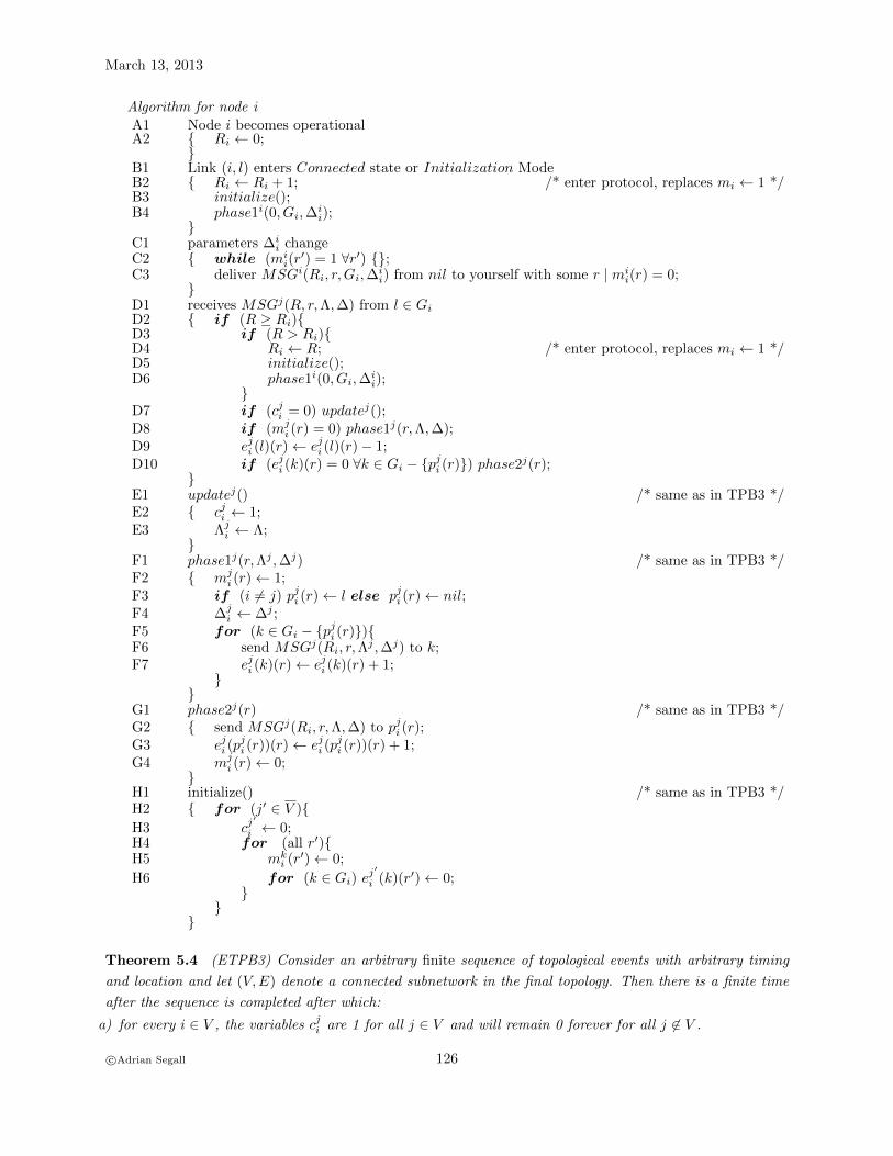
March 13, 2013
Algorithm for node iA1 Node i becomes operationalA2 { Ri ← 0;
}B1 Link (i, l) enters Connected state or Initialization ModeB2 { Ri ← Ri + 1; /* enter protocol, replaces mi ← 1 */B3 initialize();B4 phase1i(0, Gi,∆
ii);
}C1 parameters ∆i
i changeC2 { while (mi
i(r′) = 1 ∀r′) {};
C3 deliver MSGi(Ri, r,Gi,∆ii) from nil to yourself with some r | mi
i(r) = 0;}
D1 receives MSGj(R, r,Λ,∆) from l ∈ GiD2 { if (R ≥ Ri){D3 if (R > Ri){D4 Ri ← R; /* enter protocol, replaces mi ← 1 */D5 initialize();D6 phase1i(0, Gi,∆
ii);
}D7 if (cji = 0) updatej();D8 if (mj
i (r) = 0) phase1j(r,Λ,∆);D9 eji (l)(r)← eji (l)(r)− 1;D10 if (eji (k)(r) = 0 ∀k ∈ Gi − {pji (r)}) phase2j(r);
}E1 updatej() /* same as in TPB3 */E2 { cji ← 1;E3 Λj
i ← Λ;}
F1 phase1j(r,Λj ,∆j) /* same as in TPB3 */F2 { mj
i (r)← 1;F3 if (i 6= j) pji (r)← l else pji (r)← nil;F4 ∆j
i ← ∆j ;F5 for (k ∈ Gi − {pji (r)}){F6 send MSGj(Ri, r,Λ
j ,∆j) to k;F7 eji (k)(r)← eji (k)(r) + 1;
}}
G1 phase2j(r) /* same as in TPB3 */G2 { send MSGj(Ri, r,Λ,∆) to pji (r);G3 eji (p
ji (r))(r)← eji (p
ji (r))(r) + 1;
G4 mji (r)← 0;
}H1 initialize() /* same as in TPB3 */H2 { for (j′ ∈ V ){H3 cj
′
i ← 0;H4 for (all r′){H5 mk
i (r′)← 0;
H6 for (k ∈ Gi) ej′
i (k)(r′)← 0;}
}}
Theorem 5.4 (ETPB3) Consider an arbitrary finite sequence of topological events with arbitrary timing
and location and let (V,E) denote a connected subnetwork in the final topology. Then there is a finite time
after the sequence is completed after which:
a) for every i ∈ V , the variables cji are 1 for all j ∈ V and will remain 0 forever for all j 6∈ V .
c©Adrian Segall 126

Sec. 5.4
b) every i ∈ V will perform <D10>i in finite time and after the first time when it does that holds cji = 1 and
Λji = Gj for all j ∈ V and cji = 0 for all j 6∈ V .
c) suppose parameter changes at a node j ∈ V stop; a finite time afterwards every node i ∈ V will have
∆ji = ∆j
j, i.e. every node in the network will know the parameters at j and this information will never
change afterwards.
Proof: Consider the topology of the network after all topological changes cease. Consider in this topology a
given connected subnetwork (V,E). From <B2>, each topological event adjacent to a node i ∈ V increments
the cycle counter Ri at the node i adjacent to the change. Let {in} be the collection of nodes in V that
register change of status of an adjacent link, and let {tn} be the corresponding collection of times when the
status change is registered. Since there is a finite number of topological events, the collections {in}, {tn}are finite. Let R = max{Rin(tn+)} over all n. Then R is the highest cycle number ever known by nodes in
V and the cycle with number R is started by (one or more) nodes i ∈ {in} ∈ V that increment their Ri to
R as a result of a topological event. These nodes can be considered as if they receive START in the TPB3
protocol and, indeed, the network (V,E) covered by the cycle with number R registers no more topological
events, since no counter number Ri is ever increased to (R + 1). Moreover, from the Follow-up property of
DLC follows that in the final topology, l ∈ Gi if and only if i ∈ Gl, so that the assumption of bidirectionality
(Assumption a) in Sec. 3.1) holds in the final topology. Moreover, the initialization conditions for protocol
TPB3 hold why??? . Consequently, the evolution of the cycle with sequence number R is the same as in
protocol TPB3 and therefore Theorem 5.3 holds here, completing the proof. qed
Delete !!! In Protocol ETPB3, every node i ∈ V must start propagation of adjacent topology and
parameters in a PIF when it enters a new cycle of the protocol. The question is whether nodes for which
the local information has not changed since the last update was sent out, can be absolved from doing so.
The intuitive reasoning is that if the local information has not changed, then why is it necessary to send it
out again. The problem with this is however that the previous
The reason is that presumably, this is not the first time the protocol is run in the network and most
nodes have already sent out their local information. If this information has not changed since the last time it
was sent out, why is there need to send it out again. However it turns out that no initialization assumption
is sufficient, short of assuming that all nodes in V have the information. This is because if some nodes
have some incorrect old information about j and now are receiving the correct one, they have no means of
distinguishing the old ?????
have been required to start a new broadcast. The knowledge in the network could have been possible
maybe if previous to the entrance in the TPB protocol, node j has propagated the local information, after
which the information has not changed. However, maybe information from some node may already be
available at all nodes in V , maybe from previous One may ask if this is necessary if, say from previous
propagations, one can make sure that all nodes in V have
5.4 Topology and Parameter Broadcast with node-associated se-
quence numbers - Topological Changes
The protocol ETPB3 of Sec. 5.3 uses global sequence numbers R, as well as node-associated instance numbers
r. The main advantage of this method, is that, as seen in Theorem 5.4, it works under any sequence of
topological changes, including network separations and node crashes without non-volatile memory. However
the communication price to be paid to achieve this is too high: every time there is a topological change in the
c©Adrian Segall 127

March 13, 2013
network, all nodes re-broadcast their local information, even if the latter has not changed. As a result, the
more commonly used method is to employ node-associated sequence numbers only, namely to use the RPI1
protocol as described in Sec. 5.2, except that both topology and parameter information are broadcasted.
The simplistic protocol is identical to protocol TPB2 of Sec. 5.2, except that it is started by the source
node s whenever adjacent topology Gs changes as well as when adjacent parameters ∆s change and the PI1
protocol broadcasts both topology and parameter information. To recapitulate, the protocol consists of each
node incrementing its sequence number and starting a new PI1 protocol with the new sequence number,
whenever the local topology or parameters change. As in TPB2, the protocol evolves independently from
source to source and thus the superscript s is suppressed in the pseudo-code.Protocol ETPB2
Messages
MSG(r,Λ,∆) - message with sequence number r carrying the local topology and the local parametersat s (r = 0, 1, 2, . . .)
Variables
Gi - set of neighbors of node iri - largest sequence number received by i ( values 0, 1, 2, . . .)∆s - the local parameters at sΛi - list that will contain the identities of neighbors of s∆i - will contain the parameters at s as known by i
Initialization
* just before the first message is sent by s, holds rs = −1* if i receives a MSG, then
- just before receiving the first MSG, holds ri = −1
- after receiving the first MSG, node i discards and disregards messages not sent in the present instanceof the protocol
Algorithm for node iA1 node i becomes operationalA2 { ri ← 0;
}B1 when Gs or ∆s changesB2 { deliver MSG(rs + 1, Gs,∆s) from nil to yourself;
}C1 receive MSG(r,Λ,∆) from l ∈ Gi ∪ {nil}C2 { if (r > ri) phase1(r);
}D1 phase1(r) /* similar to PI1 */D2 { ri ← r ;D3 Λi ← Λ;D4 ∆i ← ∆;D5 for (k ∈ Gi) send MSG(r,Λ,∆) to k;
}
Note: In <D5>, a node i may send MSG(r,Λ,∆) to all k ∈ Gi − {l}.However, in a changing topology network, this simplistic protocol does not operate correctly. For example,
if a node fails, when it recovers, it will set its sequence number to 0. Its updates will be disregarded by other
nodes whose stored information about this node appears with a higher sequence number because of previous
updates. Only when the sequence number reaches the value that was last used before the failure will the
updates be registered.
Incorrect operation may also occur due to network disconnections and reconnections. Suppose the network
is split into two non-connected parts V ′ and V ′′. Updates initiated by nodes in V ′ do not reach nodes in V ′′.
Then, if a link connecting the two parts comes up, there is no trigger for updating nodes in V ” regarding those
c©Adrian Segall 128

Sec. 5.5
updates. The solution in existing networks, like the Internet, that uses link-state protocols in OSPF [Hui95]
is to employ periodic updates. Nodes start broadcast of topology and parameter values on a periodic basis,
even if there are no adjacent changes. This solves the disconnection problem, but does not solve the problem
of sequence number reset to 0 after a node failure. One solution for the latter problem is to use a timer
associated with each table entry and to delete entries for which updates have not been received for a long
time [Hui95],[BG92]. Moreover, messages carry an age field, and messages that are too old are discarded by
nodes.
5.5 SPTA - Topology Broadcast without sequence numbers - Topo-
logical Changes
The following protocol Shortest Path Topology Algorithm (SPTA) [BG92] allows broadcast of topology with-
out sequence numbers. The main idea is that a node believes the status of a distant link as received from
the neighbor that is on the shortest path from the node to that link.
Protocol SPTA
Messages
MSG(C) - message of the protocol (C is list of nodes whose status has changed)
Variables
Ti - main topology of node i.Ti(j) - port topology of i for neighbor node j
S(m,n)i (j) - status of link (m,n) according to port topology Ti(j) ( values up, down)
S(m,n)i - status of link (m,n) according to main topology Ti ( values up, down)Pi - a temporary group of nodes, that holds at the k-th iteration all nodes whose distance from i is nomore than k linksPi,old - the temporary group Pi from last iterationMlabeled - the group of nodes that are labeled in each iteration.Gi - set of neighbors of i, i.e. l ∈ Gi if (i, l) is in Connected state at iLabeli(j) - label of node j at node iCi - set of nodes whose status has changed
Initialization
not clear
-c©Adrian Segall 129

March 13, 2013
Algorithm for node iA1 node i becomes operationalA2 { do nothing;
}B1 link (i, l) enters Initialization Mode;
B2 { S(i,l)i ← down; S
(i,l)i (l)← down;Ci ← {((i, l), down)};
B3 for (k ∈ Gi) send MSG(Ci) to k;B4 update();
}C1 link (i, l) enters Connected State
C2 { S(i,l)i ← up; S
(i,l)i (l)← up;
C3 for (k ∈ Gi) send MSG({(i, l), up}) to k;C4 send MSG(Ti) to l;C5 update();
}D1 receives MSG(C) from l ∈ GiD2 { enter information in C into Ti(l);
D3 S(l,i)i ← up; S
(l,i)i (l)← up;
D4 update();}
E1 update()E2 { Pi,old ← i; Pi ← i; Ci ← ∅;E3 for (j ∈ Gi) {E4 Pi ← Pi ∪ {j};E5 Labeli(j) = j;
}E6 while (Mlabeled 6= ∅) {E7 Mlabeled ← ∅;E8 for (m ∈ Pi − Pi,old) {E9 for ((m,n) ∈ Ti) and (n 6∈ Pi,old)) {E10 j ← Labeli(m);
E11 if (S(m,n)i 6= S
(m,n)i (j)) Ci ← Ci ∪ ((m,n), Si(m,n));
E12 S(m,n)i ← S
(m,n)i (j);
E13 if (S(m,n)i = up) and (n 6∈ Pi)) {
E14 Labeli(n)← j;E15 Mlabeled ←Mlabeled ∪ {n};
}}
}E16 Pi,old ← Pi;E17 Pi ← Pi ∪Mlabeled;
}}
c©Adrian Segall 130

Chapter 6
DISTRIBUTED
DEPTH-FIRST-SEARCH
PROTOCOLS
Here we study Distributed Depth-First-Search Protocols. The basic protocol appears in [Che83].
Protocol DFS1
Messages
MSG - message trying to find new tree nodesREPLY - reply to MSG
Variables
Gi - set of neighbors of imi - shows if node i has already entered the protocolpi - parent of i, i.e.neighbor from which MSG was received first.vi(l) = 1 if node i knows that l has been visited; = 0 otherwise ( ∀l ∈ Gi )
Initialization
if a node i receives a MSG, then
- just before it receives the first MSG, holds mi = 0 and ci(k) = 0 for all k ∈ Gi
- after receiving the first MSG, node i discards and disregards messages not sent in the present instanceof the protocol
131

March 13, 2013
Algorithm for node i
A1 receive MSG from l ∈ Gi ∪ {nil}A2 { if (mi = 0){A3 phase1();A4 continue();
}A5 else {A6 vi(l)← 1;A7 send REPLY to l;
}}
B1 receive REPLY from lB2 { vi(l)← 1;B3 continue();
}C1 phase1()C2 { mi ← 1;C3 pi ← l; vi(pi)← 1 ;
}D1 phase2()D2 { send REPLY to pi;
}E1 continue()E2 { if (vi(k) = 1 ∀k ∈ Gi − {pi}) phase2();E3 else {E4 select any m ∈ Gi − {pi} with vi(m) = 0;E5 send MSG to m ;
}}
The properties of the DFS1 protocol are given in Theorem 6.2. Note that although the main properties
are similar to PI/PIF type protocols, the steps of the proof are somewhat different.
First note that at any given time, exactly one message travels in the network. This is because whenever
a node receives a message, it sends a message.
Lemma 6.1
a) If a node i sends a MSG to l, then from l it can receive only REPLY .
b) After a node i sends a MSG to l, the next REPLY it receives is from l.
c) No node can send two messages on the same link.
Proof: If i sends MSG to l, when the MSG arrives, then l sets vl(i) = 1, and no MSG’s are sent on
links with v = 1, hence a).
We prove b) and c) by a common induction. Let i be the first node that either receives a REPLY on a
link (i, k) on which it hasn’t last sent a MSG or that sends a second message on some link (i, j), at time t
say.
Suppose that the first kind of event happens at time t. If the message sent by i to k found mk = 1,
then k would have sent REPLY to i and the next event at i would have been to receive REPLY from k.
Therefore mk = 0 when it receives the MSG and therefore i is the parent of k. Let m be the neighbor from
which i receives REPLY at time t−. REPLY can be sent by m either in <A7> or <D2>. In both cases,
m must have previously received a MSG from i and, by the induction hypothesis, i must have received a
REPLY from m. This means that the REPLY received at time t− is a second message sent by m to i,
contradicting the second hypothesis of the common induction.
Suppose now that at time t, node i sends a second message on the same link (i, j) say. First we argue
that this message cannot be MSG. If the first message that i has sent to j was REPLY , then vi(j) was set
to 1, either at the time REPLY was sent, in <A6>, or beforehand, in <C3>. Therefore the second message
c©Adrian Segall 132

Sec. 6.0
cannot be a MSG, since such messages are sent only on links with v = 0. If on the other hand, the first
message that was sent by i to j was MSG, then by b) a REPLY was received from j before t−, which has
set vi(j)← 1 and again the second message could not be a MSG.
Therefore the message sent by i at t is a REPLY . This cannot happen as a result of i receiving at time
t− a MSG from j, since when j has received the first message from i, it has set vj(i) = 1 and nodes do not
send MSG’s on links with v = 1. Therefore j is the parent of i. When the first REPLY was sent to j, all
vi(l), l ∈ Gi − {pi} were 1, namely i has received a message on each of these links. Therefore the message
at time t is sent upon i receiving a second message on some link (i,m), meaning that m has sent a second
message on some link before time t, contradiction. qed
Lemma 6.1 implies that the protocol terminates in finite time. It can terminate only at s, since only the
parent of s is nil. It remains to show that it covers the entire network and it produces a (spanning) tree.
Theorem 6.2 (DFS1) Suppose that a node s ∈ V receives START . Recall that this is defined as the event
when s receives MSG from nil. Then:
a) all nodes i ∈ V will perform the event phase1()i in finite time and exactly once ; after this happens, the
links {(i, pi),∀i ∈ V } will form a directed spanning tree rooted at s;
b) all nodes i ∈ V will perform phase2()i in finite time and exactly once; moreover t(phase2()i) < t(phase2()pi);
node i receives no messages after time t(phase2()i); also, at the time when node s performs phase2()s, all
nodes in V have completed the algorithm, i.e. have performed phase2() and there are no messages traveling
in the network
c) exactly one message MSG or REPLY travels on each link in (V,E) in each direction.
Proof: Since this protocol simulates Tremaux’s algorithm for DFS [Eve79], all properties follow from
the properties of DFS. qed
The above protocol has 2 | E | message and time complexities. The reason is that the links are explored
serially. An improved protocol was proposed by B. Awerbuch [Awe85b]. When a node enters the protocol,
it first informs its neighbors that it has been visited. Upon receiving acknowledgment to these messages, it
continues the DFS. In this way, only the tree links are explored serially, leading to O(| V |) time complexity,
while the message complexity is only doubled to 4 | E |.Protocol DFS2
Messages
MSG - message trying to find new tree nodesREPLY - reply to MSG, or when delivered to itself, indicates that all ACK’s have been receivedV ISITED - informs neighbor that the sending node has been visitedACK - ack to V ISITED
Variables
Gi - set of neighbors of ipi - neighbor from which MSG is receivedei(k) - number of V ISITED sent - number of ACK’s received on link (i, k) ( ∀k ∈ Gi )vi(k) = 1 when i knows that neighbor k has been visited, = 0 beforehand ( ∀k ∈ Gi )
Initialization
if a node i receives MSG, then
- just before it receives the MSG, holds ei(k) = vi(k) = 0 for all k ∈ Gi
- after receiving the first MSG, node i discards and disregards messages not sent in the present instanceof the protocol
c©Adrian Segall 133

March 13, 2013
Algorithm for node i
A1 receives MSG from l ∈ Gi ∪ {nil}A2 { phase1();A3 if (Gi = {pi}) phase2();
}B1 receives REPLY from lB2 { vi(l)← 1;B3 continue();
}C1 receives V ISITED from lC2 { vi(l)← 1;C3 send ACK to l;
}D1 receives ACK from lD2 { ei(l)← ei(l)− 1D3 if (ei(k) = 0 ∀k ∈ Gi − {pi}) continue();
}E1 phase1()E2 { pi ← l;E3 for (k ∈ Gi − {pi}){E4 send V ISITED to k;E5 ei(k)← ei(k) + 1;
}}
F1 phase2()F2 { send REPLY to pi;
}G1 continue()G2 { if (vi(k) = 1 ∀k ∈ Gi − {pi}) phase2();G3 else {G4 select any m ∈ Gi − {pi} with vi(m) = 0;G5 send MSG to m ;
}}
The time complexity of DFS2 is 4 | V | −2, the message complexity is 4 | E |.
The V ISITED messages informing neighbors that a node enters the protocol are distributed in DFS2
in parallel to all neighbors. However, this is perfomed in series with the rest of the protocol. A node waits
to receive ACK’s to the V ISITED messages before proceeding to advance the protocol. The protocol
can be further improved as follows. Instead of sending V ISITED, waiting for ACK’s and then sending
MSG, a node i will send MSG to one of its neighbors, l say, and, at the same time, V ISITED to all
other non-parent neighbors. From each of the neighbors except l and pi, node i may receive V ISITED
or nothing. The response from l can be either REPLY , meaning that the parent of l is i, or V ISITED,
meaning that l has been visited before the time when l receives the MSG from i. Note that in fact node i
needs not distinguish between the two cases, since the protocol does not require nodes to know their sons.
Therefore the two types of messages can be collapsed into one, which we call V ISITED. When this message
is received, node i will send MSG to one of the neighbors from which it has received nothing, if any. If there
are no such nodes, it will send V ISITED to its parent pi. Note that with this protocol, there is no need
for ACK messages.
c©Adrian Segall 134

Sec. 6.0
Protocol DFS3
Messages
MSG - message trying to find new tree nodesV ISITED - informs neighbor that the sending node has been visited
Variables
Gi - set of neighbors of imi - shows if node i is already in the protocolpi - neighbor from which MSG is first receivedci - neighbor of i currently being investigatedvi(k) = 1 when i knows that neighbor k has been visited, = 0 beforehand ( ∀k ∈ Gi )
Initialization
if a node i receives a MSG message, then
- just before it receives the first MSG, holds mi = 0 and vi(k) = 0 for all k ∈ Gi
- after receiving the first MSG, node i discards and disregards messages not sent in the present instanceof the protocol
Algorithm for node i
A1 receives MSG from l ∈ Gi ∪ {nil}A2 { if (mi = 0) {A3 phase1();
}}
B1 receives V ISITED from lB2 { vi(l)← 1;B3 if (l = ci) { /* replaces REPLY */B4 if (current() = nil) phase2();B5 else {B6 ci ← current();B7 send MSG to ci;
}}
}C1 phase1()C2 { mi ← 1;C3 pi ← l;C4 if (current() = nil) phase2();C5 else {C6 ci ← current();C7 send MSG to ciC8 for (k ∈ Gi − {pi} − {ci}) send V ISITED to k;
}}
D1 phase2()D2 { send V ISITED to pi;
}E1 function current()E2 { if (vi(k) = 1 ∀k ∈ Gi − {pi}) current()← nil;E3 else {E4 select any m ∈ Gi − {pi} with vi(m) = 0;E5 current()← m;
}}
If all link propagation delays are the same, the time complexity of DFS3 is 2 | V | and the message
complexity is 2 | E |, the minimum possible. We don’t know the complexities for varying propagation delays.
I think it can be shown that the performance in better than DFS2.
Problems
Problem 6.0.1 Why isn’t one type of messages sufficient in DFS1?
c©Adrian Segall 135

March 13, 2013
c©Adrian Segall 136

Chapter 7
MINIMUM-WEIGHT SPANNING
TREE PROTOCOLS
In this chapter we investigate the Minimum Spanning Tree protocol of Gallager, Humblet and Spira [GHS83].
Protocol MST
MessagesConnect(Z) -Initiate(Z,F, S) -Test(Z, S) -Accept -Report(w) -ChangeRoot -
VariablesGSH notation
si - state of node i SN- Sleeping = initial state- Find = participating in search for minimum outgoing edge- Found = at other times
si(l) - state of link (i, l) as seen by i SE(m)- Basic = unknown yet- Branch = edge is branch in MST- Rejected= edge is non-branch connecting two tree nodes
Fi - fragment identityZi - fragment level LNBestEdgei - edge pointing towards minimum-weight outgoing edgeBestWti - weight of minimum-weight outgoing edgeTestEdgei - adjacent edge currently being testedpi - branch pointing towards core in− branchFindCounti - Number of Report messages to be receivedwi(l) - weight of link (i, l) w(j)
Initialization
In the beginning :si = Sleeping
137

March 13, 2013
Algorithm for node iA1 Node i wakes upA2 { wakeup()
}B1 wakeup()B2 { ∀ adjacent l, set si(l)← Basic;B3 BestEdgei ← adjacent edge of minimum weight;B4 BestWti ← w(BestEdgei) ; Zi ← 0 ; si ← Found ;B5 FindCounti ← 0 ; pi ← nil; @B6 ChangeRoot() ; @
}C1 receives Connect(Z) on edge jC2 { if (si = Sleeping) wakeup() ;C3 if (Z < Zi) { Z ≤ Zi, see item 3) belowC4 si(j)← Branch;C5 send Initiate(Zi, Fi, si) on edge j;C6 if (si = Find)FindCounti ← FindCounti + 1;
}C7 elseif (si(j) = Basic) place message on end of queue ;wait for until i completes building the tree and changes si(j) to BranchC8 else {C9 send Initiate(Zi + 1, w(j), F ind) on edge j;
}}
D1 receives Initiate(Z,F, s) on edge j Z > ZiD2 { Zi ← Z ; Fi ← F ; si ← s; pi ← j ;D3 BestEdgei ← nil; BestWti ←∞ ;D4 ∀m 6= j such that si(m) = Branch {D5 send Initiate(Z,F, s) on edge m ;D6 if (s = Find) FindCounti ← FindCounti + 1 ;
}D7 if (s = Find) test() ;
}E1 test()E2 { TestEdgei ← minimum-weight adjacent edge in state Basic ;E3 send Test(Zi, Fi) on TestEdgei ;E4 report() ;
}F1 receives Test(Z,F ) on edge jF2 { if (si = Sleeping) wakeup() ;F3 if (Z > Zi) place message on end of queue ; wait to get to higher levelF4 elseif (F 6= Fi) send Accept on edge j ; what if Z < Zi ??F5 else { same fragmentF6 if (si(j) = Basic) si(j)← Rejected;F7 if (TestEdgei 6= j) send Reject on edge j ;F8 else test() ; check this
}}
c©Adrian Segall 138
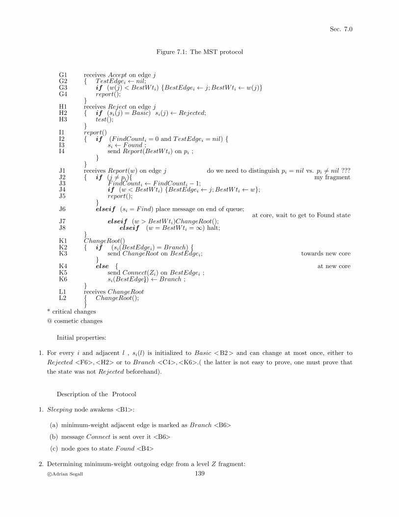
Sec. 7.0
Figure 7.1: The MST protocol
G1 receives Accept on edge jG2 { TestEdgei ← nil;G3 if (w(j) < BestWti) {BestEdgei ← j;BestWti ← w(j)}G4 report();
}H1 receives Reject on edge jH2 { if (si(j) = Basic) si(j)← Rejected;H3 test();
}I1 report()I2 { if (FindCounti = 0 and TestEdgei = nil) {I3 si ← Found ;I4 send Report(BestWti) on pi ;
}}
J1 receives Report(w) on edge j do we need to distinguish pi = nil vs. pi 6= nil ???J2 { if (j 6= pi){ my fragmentJ3 FindCounti ← FindCounti − 1;J4 if (w < BestWti) {BestEdgei ← j;BestWti ← w};J5 report();
}J6 elseif (si = Find) place message on end of queue;
at core, wait to get to Found stateJ7 elseif (w > BestWti)ChangeRoot();J8 elseif (w = BestWti =∞) halt;
}K1 ChangeRoot()K2 { if (si(BestEdgei) = Branch) {K3 send ChangeRoot on BestEdgei; towards new core
}K4 else { at new coreK5 send Connect(Zi) on BestEdgei ;K6 si(BestEdgei) ← Branch ;}
}L1 receives ChangeRootL2 { ChangeRoot();
}* critical changes
@ cosmetic changes
Initial properties:
1. For every i and adjacent l , si(l) is initialized to Basic <B2> and can change at most once, either to
Rejected <F6>,<H2> or to Branch <C4>,<K6>.( the latter is not easy to prove, one must prove that
the state was not Rejected beforehand).
Description of the Protocol
1. Sleeping node awakens <B1>:
(a) minimum-weight adjacent edge is marked as Branch <B6>
(b) message Connect is sent over it <B6>
(c) node goes to state Found <B4>
2. Determining minimum-weight outgoing edge from a level Z fragment:
c©Adrian Segall 139

March 13, 2013
(a) Core nodes start broadcasting Initiate(Z,F, s) messages <C8>
(b) Initiate(Z,F, F ind) messages are sent outward on the fragment branches <D5> and to lower level
fragments <C5> (in the paper it says layer (L − 1), but it’s not clear that indeed this is the case
in <C3> ). For every Initiate message sent, a node expects a Report message back. The variable
FindCounti keeps track of the number of Initiate’s sent minus the number of Report’s received.
(c) A node finds its minimum-weight outgoing edge via Test/Reject/Accept messages (see 6) below).
(d) Nodes collaborate via Report messages converging to the core node <I4> to find the minimum-weight
fragment outgoing edge. BestEdge is saved and nodes go into Found state.
3. Receipt of Connect
(a) A sleeping node i can receive Connect only if the sending node k has sent it upon its own wakeup,
otherwise k has previously sent Test to i, which would have woken i up.
(b) Upon entering <C3> holds Z ≤ Zi. This is because of the following:
• If Zi = 0, then Z = 0 as explained above.
• If Zi > 0, then Z cannot be larger than Zi because the sending node k has previously sent Test
to i and that Test would have been placed on the end of queue in <F3> until Zi would reach the
level of Z.
4. Changing the core
(a) The two core nodes exchange Report <I4>. When a core node receives Report, it waits, if necessary,
to get into state Found <J6>. The core node with the lower BestWt, starts <J7> propagation of
ChangeRoot towards minimum-weight edge <K3>.
(b) When the ChangeRoot message reaches the node adjacent to the minimum-weight outgoing edge, the
(i, pi) edges form a rooted tree, rooted at this node.
(c) When the ChangeRoot message reaches the node adjacent to the minimum-weight outgoing edge, the
node with the minimum-weight outgoing edge sends a Connect(Z) message over this edge <K5>.
(d) If two fragments at level Z have the same minimum-weight outgoing edge, each sends Connect(Z) over
the edge, which causes the edge to become a Z + 1-level core <C9>
5. Connecting a low-level fragment to a high-level one <C3>
(a) Suppose node i in fragment Fi with level Zi sends a Connect message to node i′ in fragment F ′ with
level Zi′ , where Zi′ > Zi. When it receives the Connect message, node i′ responds with an Initiate
message <C5>.
(b) If i′ is in state Find, the low-level fragment joins the search for the minimum-weight outgoing edge <
C6>. If i′ is in state Found, we can deduce that an outgoing edge from node n′ has a lower weight
than the minimum-weight outgoing edge from Fi. Thus there is no need for fragment Fi to join the
search. (??? Is it possible that edge (i, i′) is the minimum-weight outgoing edge from Fi ? Is there a
problem in this case ? Maybe it works, but it is not the normal operation as described in the paper.)
6. Finding minimum-weight outgoing edge at a node (test() procedure, <E1>)
(a) starts when node i receives Initiate in state Find, <D7>, at which time node i sends Test(Zi, Fi) on
its minimum-weight adjacent edge in state Basic
c©Adrian Segall 140

Sec. 7.0
(b) At the receiving node, if the node’s level Zi is less than the received level Z, the node delays making
any response <F3>.
(c) Otherwise, if the receiving node is not in the same fragment as the sending node, Accept is sent back
to the sending node <F4>.
(d) Otherwise, the link is put in Rejected state and, if Test was not previously sent on this link by the
receiving node, the latter sends Reject back. (Note: Probably the Test and Reject messages can be
combined in one, in <F7>, the node can send Test(Zi, Fi) and the procedure for Reject can be deleted.
c©Adrian Segall 141

March 13, 2013
c©Adrian Segall 142

Chapter 8
MINIMUM-HOP-PATH
PROTOCOLS
In previous chapters, we have presented protocols for propagation of information in networks. In particular,
we developed in Chap. 5 protocols like Topology and Parameter Broadcast, which require nodes to distibute
to all network nodes their local topology and adjacent parameters. The result is that all nodes maintain
a map of the entire network, allowing them to participate in routing protocols of the link state type, like
the Internet OSPF [Hui95]. Another method for routing in communication networks, including the Internet,
is Distance Vector [Hui95]. With this method, nodes do not maintain the entire network topology. They
keep only a table of the estimated next-hop and estimated shortest distance to each other destination in the
network. By exchanging these table with the neighbors, nodes update their own tables. In the present and
the following chapters, we shall discuss such protocols. The present chapter assumes unity-weights on all
links, so that we are looking for minimum-hop protocols, while Chapter 9 deals with protocols for networks
with variable link weights.
8.1 Protocol MH1
The problem considered next is to obtain the paths with smallest number of links (hops) from each node to
each other node. As before, at the beginning of the algorithm a node knows only its own identity and the
adjacent links. When the algorithm is completed at a node i, we want the node to know its distance dki in
terms of number of links to all other nodes to which it is connected and a preferred neighbor pki through which
it has the minimum-hop path to k. Observe that we do not require nodes to know the entire minimum-hop
path.
If the travel time of control messages were identical on all links, then we could have accomplished
the minimum-hop-path by using protocol PI1 (see Theorem 3.1c)). However, as stated before, such an
assumption is not practical, and the problem is to design a Distributed Network Protocol where nodes will
receive the first message with a given identity from the neighbor providing the shortest path, even if link
delays are arbitrary. Such a protocol has been proposed by Gallager [Gal76], [Gal82].
A node enters the algorithm in the same way as in the CT protocols, namely when receiving START or
the first control message, at which time it knows its own identity and the identity of all its neighbors, i.e.
all nodes that are at distance 0 and 1 from itself. At that time it sends the identity of its neighbors to all
neighbors. After having received the identity of the neighbors of all its neighbors, node i knows all nodes
143

March 13, 2013
that are at distance 2 from it. Node i keeps the information, sends it to all neighbors and then waits to
receive the lists of all nodes that are at distance 2 from each of its neighbors. The union of these lists minus
the set of nodes already known to i, i.e. those that are at distance 0,1 or 2 from it, is exactly the set of nodes
that is at distance 3 from i. This information is kept again at i and also distributed to neighbors, and the
procedure is repeated. If at some level, the union of the lists received from all neighbors contains no nodes
that are unknown to i, then node i has completed the algorithm. It sends to all neighbors a message saying
that it has no new node identities to send and stops. Any further message it may receive is disregarded.
Protocol MH1
Messages
MSG(LISTi) - message sent by node iSTART - MSG(∅) from nil
Variables
dki - distance from i to k; set initially to | V | for all k (values 0, 1, . . . | V |)pki - preferred neighbor of i for k, for all kZi - state of node i showing distance covered by the protocol up to now (values 0, 1, . . . , | V | −1)mi - shows if node i is currently participating in the protocol (values 0, 1)Ni(l) - level of last message received on link (i, l) (values 0, . . . , | V | −1), for l ∈ Gi
Initialization
- just before node i enters the protocol, it has Zi = 0.- after entering the protocol, node i discards and disregards messages not sent in the present instanceof the protocol
c©Adrian Segall 144

Sec. 8.1
Algorithm for node i
A1 receive MSG(LIST ) from l ∈ Gi ∪ {nil}A2 { if (Zi = 0){A3 initialize();A4 level();
}A5 if (mi = 1){A6 update();A7 if (Zi ≤ Ni(l
′) ∀l′ ∈ Gi) level();}
}B1 initialize()B2 { for (k ∈ V ){B3 dki ←| V |;B4 pki ← nil;
}B5 for (l′ ∈ Gi) Ni(l
′)← 0;B6 mi ← 1;B7 dii ← 0;B8 for (k ∈ Gi){B9 dki ← 1;B10 pki ← k;
}}
C1 update()C2 { Ni(l)← Ni(l) + 1;C3 for (k ∈ LIST ){C4 if (dki > Ni(l) + 1){C5 dki ← Ni(l) + 1;C6 pki ← l;
}}
}D1 level()D2 { Zi ← Zi + 1;D3 LISTi ← {k | dki = Zi};D4 for (k ∈ Gi) send MSG(LISTi) to k;D5 if (LISTi = ∅) mi ← 0;
}
Note: Observe that the variable pki is not needed by the algorithm, and only designates the neighborcorresponding to the minimum hop path to k.At first glance it seems that we could use the concept of synchronizers of [Awe85a] to prove the properties
of Protocol MH1. The time when Zi ← n, n = 1, 2, . . . could be taken as the synchronizer time ti(n). The
MSG sent by i to all neighbors at that time could be taken as SY NCHn in synchronizer α given in
[Awe85a]. However, as seen in Lemma 8.2, these sequences of instances do not satisfy a basic property
required in [Awe85a], that a MSG sent by i at ti(n) can arrive at a neighbor k before tk(n). Therefore
there is no synchronizer for this protocol and hence the proof must be carried out directly.
The following definition and theorem summarize the main properties of the protocol.
Definition: The number of links on the minimum-hop path from i to k is called the hop-distance from
i to k.
Theorem 8.1 (MH1) Suppose START is delivered to a node (or several nodes) in V . Then every node
i ∈ V :
a) will enter the protocol (i.e. perform <A2>) in finite time;
b) will complete the protocol (i.e. perform <D5>) in finite time, with dki , pki corresponding to the minimum-
hop path from i to k for all nodes k ∈ V and with dki =| V |, pki = nil for all nodes k 6∈ V .
c©Adrian Segall 145

March 13, 2013
Proof: The proof is given in the following two lemmas. The first indicates several preliminary properties of
protocol MH1 connected to message exchanges and variable updates, while in the second we use Lemma 8.2
to validate the basic properties of the protocol.
Lemma 8.2 Suppose START is delivered to a node (or several nodes) in V . Then for any i ∈ V holds:
a) i will enter the protocol in finite time;
b) messages are sent by node i if and only if Zi is incremented at the same time; if MSG is sent by i while
Zi ← Z, receipt of the MSG at neighbor l will cause Nl(i)← Z;
c) Zi and Ni(m) for each m ∈ Gi change only by increments of +1;
d) for each m ∈ Gi, holds Ni(m) = Zi or Zi ± 1 and there is at least one m for which Ni(m) = Zi − 1 (note:
this implies Zi = minmNi(m) + 1);
e) no message can arrive on links (i,m) for which Ni(m) = Zi + 1;
f) if Zi is incremented at time t, then for all m ∈ Gi holds Ni(m)(t+) = Zi(t+) or Zi(t+)− 1.
Proof: Part a) holds since propagation of <A2> happens as /phase1/ in PI1. Assertion b) holds since Zi
is incremented whenever MSG is sent (<D2>,<D4>), Ni(l) is incremented whenever MSG is received from
l(<C2>) and both are initialized to 0. In addition, c) follows from <D2>. Property d) is true immediately
after the time when node i enters the algorithm, at which time either Zi = 1 and minmNi(m) = 0, or Zi = 2
and minmNi(m) = 1, the latter if i has only one neighbor and enters the algorithm by receiving MSG from
it. Suppose now that the property is true at node i up to time t− and we want to show that it will hold at
time t+ as well. The variables Ni(•) or Zi can change at time t only if a MSG is received, from neighbor l
say. Let Zi(t−) = Z. We have several cases:
i) Ni(l)(t−) = Z − 1 and ∃m 6= l with Ni(m)(t−) = Z − 1; then Ni(l)(t+) = Zi(t+) = Z and all other
Ni(•) do not change, hence d) continues to hold at time t+.
ii) Ni(l)(t−) = Z − 1 and 6 ∃m 6= l with Ni(m)(t−) = Z − 1; then Ni(l)(t+) = Z and Zi(t+) = Z + 1, since
<A7> holds at t, and d) continues to hold at t+.
iii) Ni(l)(t−) = Z, in which case Ni(l)(t+) = Z+ 1 and Zi(t+) = Z, hence d) continues to hold at time t+.
iv) We claim that Ni(l)(t−) cannot be Z+1. Suppose Ni(l)(t−) = Z+1. Then Ni(l)(t+) = Z+2, and from
b) follows that at time t1 < t, node l has sent MSG(LISTl) while Zl = Z + 2. From <A7>, <D2>,<D4>
we have Zl(t1−) = Z + 1 and Nl(i)(t1+) ≥ Z + 1. This means that ∃t2 < t1 when i has sent MSG(LIST )
to l, while Zi(t2+) = Z + 1. But the latter and Zi(t−) = Z contradicts the monotonicity of Zi (see c)).
This completes the proof of d). Observe now that e) is exactly case iv) in d). Finally, observe that
scanning cases i)-iv) of d), we see that Zi is incremented only in case ii) and f) clearly holds in this case,
completing the proof of the lemma. qed
Lemma 8.3 Recall the definition of the term hop-distance just before Theorem 8.1. Under the same
conditions as in Lemma 8.2 holds:
a) If a node i has nodes at hop-distance r, then it sets Zi ← r in finite time and then sends MSG(LISTi),
where LISTi contains exactly all nodes k that are at hop-distance r; for all those nodes holds dki = r and pki= first link on minimum-hop path to k and these dki , pki are final.
c©Adrian Segall 146

Sec. 8.1
b) Let Si be the largest hop-distance from node i in the network, i.e. node i does have nodes at hop-distance
Si, but has no nodes at hop-distance (Si + 1); then node i will set Zi ← (Si + 1) in finite time, at which time
it sends MSG(LISTi) with LISTi = ∅ and performs <D5>; node i will not increase Zi any further.
Proof: Setting of Zi ← 1 while sending MSG(LISTi) with LISTi = {Gi} propagates as in PI1 and hence
will happen at all nodes in finite time. Now suppose a) holds for all nodes that have nodes at hop-distance
(r − 1). Consider a node i that has nodes at hop-distance r. Then itself and all its neighbors m have nodes
at hop-distance (r − 1) and by the induction hypothesis, they set Zm ← (r − 1) and send MSG(LISTm).
When such a message arrives at i, it sets Ni(m) ← (r − 1) and after all such messages arrive, <A7> will
hold with Zi = (r − 1). This causes Zi ← r. At this time we have from Lemma 8.2f), Ni(m) = r or (r − 1)
for all m.
Now suppose k is at hop-distance r from i. Then there is a neighbor m of i such that k is at hop-distance
(r−1) from m and there is no neighbor m of i such that k is at hop-distance strictly less than (r−1) from m.
By the induction hypothesis, k was sent by m in MSG(LISTm) while Zi ← (r − 1) and hence was received
at i while Ni(m) ← (r − 1), but was sent by no neighbor m′ while Zm′ ← Z < (r − 1). Hence at the time
Zi ← r we have dki = r, and therefore k is sent in MSG(LISTi). From <C5>,<C6> it is clear that this dkiand the corresponding pki are final and correct. A similar argument shows that nodes at hop-distance other
than r cannot be included in the LISTi considered above. This completes the proof of a).
First consider a node i s.t. Si = min{Sj} where the min is over all nodes in the network. All its
neighbors m have nodes at distance Si and by a) they send MSG(LISTm) while Zm ← Si. When all these
messages arrive to i, Zi will become Si + 1, but since i has no nodes at hop-distance Si + 1, holds LISTi = ∅and hence i performs <D5>. Now suppose by induction that b) holds for all nodes i for which Si ≤ S − 1.
Consider a node j with Sj = S. Node j has a node k at hop-distance S and k is included in LISTj when j
sends MSG(LISTj) while Zj ← S. We need to show that Zj will eventually take on value (S + 1). First
we show that for all neighbors m of j, Zm will become S. For an arbitrary neighbor m of j, node k is at
hop-distance (S − 1), S or (S + 1) from m and hence Sm ≥ S − 1. If Sm ≥ S, then a) implies that Zm will
become S in finite time. If Sm = S− 1, then Zm will become S in finite time from the induction hypothesis.
Hence from Lemma 8.2b), Nj(m) will become S in finite time for all neighbors m of j and hence Zj will
become (S + 1). Since j has no nodes at hop-distance (S + 1), <D5> will hold and this completes the proof
of the lemma. qed
Now, Lemma 8.2a) and Lemma 8.3a),b) are exactly Theorem 8.1 and this completes the proof of the
Theorem.
Communication cost: From the proof of Theorem 8.1 follows that the identity of every node travels
exactly once on each link, and hence we need | V | log2 | V | bits on each link in each direction, for a total
of 2 | E || V | log2 | V | bits.
Time complexity = O(| V |2)
Computation ????
Problems
Problem 8.1.1 * Wrong Initial Conditions
Problem 8.1.2 Consider a network with nodes a, b, c, d, s and links and delays (in both directions) as
follows:Link a,b a,c a,s b,c b,d c,d c,s d,s
Delay 3 5 3 3 2 2 1 6The nodes in this network perform MH1. Node s
receives START at t = 0.
1. Give the sequence of messages received at s, and the sequence of messages sent by s.
c©Adrian Segall 147

March 13, 2013
2. When does the protocol complete?
3. Give the tables at each node when the protocol completes?
Problem 8.1.3 Suppose that after an execution of the MH1 protocol is completed at all nodes, a new link
goes up between nodes i and j (the network was connected before this event).
a) Explain and prove how can i and j exchange only one message to update their tables (namely, to update
pki , dki , p
kj , d
kj for all k ∈ V .
b) Under what condition on the new and old tables of i and j are the tables of all other nodes correct in
spite of the link addition?
Problem 8.1.4 a) Give an upper bound on the number of messages a node can receive after performing
<D5>. What can be said on their contents? Are the LIST’s of those messages necessarily empty?
b) Prove or give counterexample: Every node receives at least one MSG after performing <D5>.
c©Adrian Segall 148

Sec. 8.2
8.2 Extending MH1 to changing topologies
change section name check Lamport, Time,Clocks,.. 1978 As with CT protocols, MH1 requires spec-
ified initial conditions and therefore its extension to handle topological changes must include reinitialization
after every such change. This is implemented as in Sec. 4.6 by restarting a new cycle of the protocol after
every topological event. The cycles of the protocol will be labeled with increasing numbers, every node re-
members the highest cycle number known to it so far and each of the cycles corresponds now to the original
(nonextended) protocol. When a node wants to trigger a new cycle due to an adjacent topological event, it
resets its variables, increments the cycle number and acts as if it has received START for a new cycle with
this number. Here resetting variables means to adjust the appropriate variables to their required initial value
as stated in the corresponding assumption in each of the protocols (e.g. in MH1, pki ← nil, dki ←| V | for all
k and Zi ← −1, Ni(m)← −1 for all m ∈ Gi). The number of the new cycle will be carried by all messages
belonging to this cycle and now, any node receiving a message with cycle numbers lower than the one known
to it so far discards this message. A node receiving a message with higher cycle number than the highest
known to it, resets its own variables, increases its registered maximal cycle number accordingly and acts as if
it enters the protocol now (i.e. the corresponding cycle of the extended protocol). In this way the cycle with
higher number will cover the lower-number cycles, in the sense that when a higher cycle reaches any node,
the node will forget the previous knowledge and will participate only in the most recent cycle. Observe that
several nodes may start the same new cycle independently because of multiple topological events, but the
protocol allows this situation to happen, considering it in the same way as if several nodes receive START
in the nonextended protocol.
???? There is a question, whether it is indeed necessary for all nodes to forget their entire previous
knowledge, as opposed to protocols where only the information affected by the topological change is discarded,
while the rest of the network adapts smoothly to the new situation. For the PU protocol, such a protocol
appears in [xxx], [yyy], [zzz], but for the others this is still an open question. ?????
As an example, we shall write exactly the extended MH1 protocol.
Protocol EMH1
Messages
MSG(R,LIST ) message
Variables
Gi - set of neighbors of i, i.e. k ∈ Gi if (i, k) is in Connected state at idki - distance from i to kpki - preferred neighbor from i to k for all kZi - state of node i showing distance covered by the protocol up to now (values 0, 1, . . . , | V | −1)mi - shows if node i is currently participating in the protocol (values 0,1)Ni(l) - level of last message received on link (i, l) (values 0, . . . , | V | −1), for l ∈ Gi
Ri - highest sequence number known to i (values: 0,1, . . . );c©Adrian Segall 149

March 13, 2013
Algorithm for node iA1 node i becomes operationalA2 { Ri ← 0;
}B1 link (i, l) enters Connected state or Initialization ModeB2 { Ri ← Ri + 1; /* enter protocol */B3 Zi ← 0;B4 initialize();B5 level();
}C1 receives MSGj(R,Λ) from l ∈ GiC2 { if (R ≥ Ri){C3 if (R > Ri){C4 Ri ← R; /* enter protocol */C5 Zi ← 0;C6 initialize();C7 level;
}C8 if (mi = 1){C9 update();C10 if (Zi ≤ Ni(l
′) ∀l′ ∈ Gi) level();}
}}
D1 initialize()D2 { for (k ∈ V ){D3 dki ←| V |;D4 pki ← nil;
}D5 for (l′ ∈ Gi) Ni(l
′)← 0;D6 mi ← 1;D7 dii ← 0;D8 for (k ∈ Gi){D9 dki ← 1;D10 pki ← k;
}}
E1 update()E2 { Ni(l)← Ni(l) + 1;E3 for (k ∈ LIST ){E4 if (dki > Ni(l) + 1){E5 dki ← Ni(l) + 1;E6 pki ← l;
}}
}F1 level()F2 { Zi ← Zi + 1;F3 LISTi ← {k | dki = Zi};F4 for (k ∈ Gi) send MSG(Ri, LISTi) to k;F5 if (LISTi = ∅) mi ← 0;
}Note that <B1> and <C3> here correspond to <A2> in MH1. The properties of EMH1 are:
Theorem 8.4 (EMH1) Consider an arbitrary finite sequence of topological events with arbitrary timing
and location and let (E, V ) denote a connected subnetwork in the final topology. Then there is a finite time
after the sequence is completed after which no messages travel in (V,E) and all nodes i ∈ V will have mi = 1
with the same cycle number Ri, with correct dki and pki for all k ∈ V and with dki =| V |, pki = nil for all
k 6∈ V .
Proof: From <B2>, each topological event increments the cycle counter Ri at the node i adjacent to the
c©Adrian Segall 150

Sec. 8.2
change. Let {in} be the collection of nodes that register change of status of an adjacent link, and let {tn}be the corresponding collection of times when the status change is registered. Since there is a finite number
of topological events, the collections {in}, {tn} are finite. Let R = max{Rin(tn+)} over all n. Then R is the
highest cycle number ever known in the network and the cycle with number R is started by (one or more)
nodes i ∈ {in} that increment their Ri to R as a result of a topological event. These nodes can be considered
as if they receive START in the MH protocol and, indeed, the network covered by the cycle with number
R registers no more topological events, since no counter number Ri is ever increased to (R + 1). Moreover,
from the Follow-up property of DLC follows that in the final topology, l ∈ Gi if and only if i ∈ Gl, so that
the assumption of bidirectionality (Assumption a) in Sec. 3.1) holds in the final topology. Consequently, the
evolution of the cycle with sequence number R is the same as in protocol MH1 and therefore Theorem 8.1
holds here, completing the proof.
Problems
Problem 8.2.1 In a network with all delays constant and equal to 1, can we use bounded sequence numbers
in EMH1?
Problem 8.2.2 Does EMH1 work in a network where all parts of data reliability properties, except for
crossing , hold?
Problem 8.2.3 Consider a network with nodes a, b, c, d, e, links and delays (in both directions) as follows:
a,b - 3
a,c - 5
a,e - 3
b,c - 3
c,d - 2
c,e - 4
d,e - 2
Suppose all nodes come up and all links enter connected state at time t = 0, and afterwards the following
happen :
At time t = 5 link (a, b) fails and both ends enter Initialization state.
At time t = 9 link (e, c) enters Initialization state at node e.
At time t = 10 link (e, c) enters Initialization state at node c, and link (a, b) enters connected state at node
a.
At time t = 12 link (e, c) enters connected state at node c, and link (a, b) enters connected state at node b.
At time t = 15 link (e, c) enters connected state at node e and no more topological changes happen afterwards.
The nodes perform EMH1:
1. Indicate the values of the variables (Gi, dki , p
ki , Zi, Ri) as a function of time at each node.
2. At what time are there no messages traveling in the network?
3. What is the highest sequence number reached by the network? Suggest other timings for the same topological
changes in order to get a higher maximal sequence number, suggest timings to get a lower maximal sequence
number.
Problem 8.2.4 Specify the code of ECT5 (protocol CT5 extended to handle topological changes using
sequence numbers).
c©Adrian Segall 151

March 13, 2013
8.3 Another Version (MH2)
A slight change in Protocol MH1 [Gal82] reduces the time complexity from O(| V |2) to O(| V |), without
affecting the communication cost. Instead of collecting the identities of all nodes at a given distance and
send them in one message, we send the identities in separate messages as they become available. To enable
neighbors to distinguish between levels, after having sent all identities of nodes at a given distance, a node
sends a SY NCH message to all neighbors.
Protocol MH2
Messages
MSG(k) - message sent by node i with identity of node kSY NCH - message designating beginning of new levelSTART - SY NCH from nil
Variables
dki - distance from i to k; set initially to | V | for all k (values 0, 1, . . . | V |)pki - preferred neighbor of i for k for all kZi - state of node i showing distance covered by the protocol up to now (values −1, 0, 1, . . . , | V | −1)mi - shows if node i is currently participating in the protocol (values 0, 1)Ni(l) - level of last message received on link (i, l) (values −1, 0, . . . , | V | −1), for l ∈ Gi
L - shows if messages MSG have been sent since Zi was last incremented
Initialization
- just before node i enters algorithm, holds Zi = −1- after entering the protocol, node i discards and disregards messages not sent in the present instanceof the protocol
c©Adrian Segall 152

Sec. 8.3
Algorithm for node i
A1 receive SY NCH from l ∈ Gi ∪ {nil}A2 { if (Zi = −1){A3 initialize();A4 level();
}A5 if (mi = 1){A6 Ni(l)← Ni(l) + 1;A7 if (Zi ≤ Ni(l
′) ∀l′ ∈ Gi) level();}
}B1 receive MSG(k) from l ∈ Gi ∪ {nil}B2 if (mi = 1) update();
}C1 initialize()C2 { for (k ∈ V ){C3 dki ←| V |;C4 pki ← nil;
}C5 for (l′ ∈ Gi) Ni(l
′)← −1;C6 mi ← 1;C7 L← 1;C8 dii ← 0;C9 for (k ∈ Gi){C10 dki ← 1;C11 pki ← k;
}}
D1 update()D2 { if (dki > Ni(l) + 1){D3 dki ← Ni(l) + 1;D4 pki ← l;
}D5 if (dki = Zi + 1){D6 for (l′ ∈ Gi) send MSG(k) to l′;D7 L← 1;
}}
E1 level()E2 { Zi ← Zi + 1;E3 for (k ∈ Gi) send SY NCH to k;E4 if (L = 0) mi ← 0;E5 else L← 0;E6 for (k′ | dk′i = Zi + 1){E7 for (l′ ∈ Gi) send MSG(k′) to l′;E8 L← 1;
}}
Problems
Problem 8.3.1 How do Lemmas 8.2 and 8.3 change when proving MH2?
c©Adrian Segall 153

March 13, 2013
8.4 The Fixed Topology Distributed Bellman-Ford Minimum Hop
Protocol (MH3)
This protocol establishes minimum hop paths from all nodes in the network to a given destination s. A
node i keeps an estimate di of its shortest path to the destination and estimates Di(l) of the shortest path
via each neighbor l. When the estimate di changes, i sends a message containing the new estimate to all
neighbors. When i receives a message from a neighbor l, it updates its estimate Di(l) of the shortest path
via that neighbor and its estimate di of its shortest path to the destination. If the new di is different from
the old one, a message containing the new value is sent to all neighbors. The distance from a node i to s
can be no larger than | V | −1, where | V | is the maximum number of nodes potentially in the network.
It is shown that a finite time after the protocol is started, it terminates. At that time, all nodes in V have
correct estimated distances: if s ∈ V , then all di ≤| V | −1 and are correct; if s 6∈ V , then all di =| V |. In
practice, the protocol is repeated independently for every destination s. Also, to save overhead, messages
belonging to several protocols (for different destinations) may be combined in one message.
This is the ARPA-1 routing protocol [MW77], specialized to the case when link weights are 1, except that
the updates are performed on an event driven basis rather than periodically. It is also the fixed topology
part of the 1 MERIT network routing protocol [Taj77].Protocol MH3
Messages
MSG(d) - message sent by node i, containing i’s estimated distance to s, (values 0, 1, . . . , | V |)
Variables
di - estimated distance from i to s (values 0, 1, . . . , | V |)pi - preferred neighbor of iDi(l) - estimated distance from i to s via neighbor l, (values 0, 1, . . . , | V |)
Initialization
holds ds = 0 and for all i 6= s and l ∈ Gi, the variables di and Di(l) satisfy:
a) di = min Di(l′) over l′ ∈ Gi
b) Di(l) = min (dl + 1, | V |) or there is at least one MSG on (l, i) and the last MSG(d) on (l, i)contains d = dl
Note: an example of a set of variables and messages that satisfy the above is: di = Di(l) =| V | for alli 6= s and all l ∈ Gi, there is a MSG(0) on all links (s, l), for all l ∈ Gs and there is no MSG after it.
Algorithm for node sA1 do nothing
Algorithm for node i 6= s
B1 receive MSG(d) from l ∈ Gi
B2 { Di(l)← min(d+ 1, | V |);B3 update();
}C1 update()C2 { k∗ ← node that achieves minDi(l
′) over l′ ∈ Gi;C3 if (di 6= Di(k∗)) {C4 pi ← k∗;C5 di ← Di(k∗);C6 for (k ∈ Gi) send MSG(di) to k;
}}
1introduce periodical updates
c©Adrian Segall 154

Sec. 8.4
Lemma 8.5 At all times holds ds = 0 and for all i 6= s and l ∈ Gi, the variables di and Di(l) satisfy:
a) di = min Di(l′) over l′ ∈ Gi
b) Di(l) = min (dl + 1, | V |) or there is at least one MSG on (l, i) and the last MSG(d) on (l, i) contains
d = dl
c) all variables di, Di(k) take on values between 0 and | V |; all messages MSG(d) contain 0 ≤ d ≤| V |
Proof: Note that ds stays 0 forever and a) and c) are obviously correct. To prove part b), consider a node i
and some l ∈ Gi. Recall from assumption a) in Sec. 3.1 that l ∈ Gi if and only if i ∈ Gl. Then b) is correct
at initialization by assumption and if l changes its estimated distance dl, it sends a MSG(dl) to all nodes in
Gl, and in particular on (l, i). By FIFO, unless l changes again its dl, this is the last MSG on (l, i), until it
arrives at i, in which case the latter sets Di(l) = min (dl + 1, | V |). qed
Theorem 8.6 (MH3) There is a finite time after which no messages travel in (V,E) and: i) if s ∈ V , then
all nodes i ∈ V have di = shortest hop distance to s and pi = first link on the minimum hop path to s; ii) if
s 6∈ V , then all nodes i ∈ V have di =| V |.
Proof: We prove the theorem via several lemmas.
Lemma 8.7 If all message activity ceases, then the di, Di(l), pi entries are correct for all i ∈ V and all
l ∈ Gi.
Proof: Suppose first that s ∈ V . For i ∈ V , let
d∗i = shortest hop distance from i to s
K = set of nodes in V for which di < d∗i
j = node in K with minimum di, i.e. holds dj ≤ di,∀i ∈ K
Since there are no messages on the links, Lemma 8.5 implies that dj = Dj(pj) = dpj+ 1, hence pj 6∈ K,
so dpj≥ d∗pj
. But since j and pj are neighbors, the triangle inequality implies that d∗j ≤ d∗pj+ 1. Hence,
dj = dpj+ 1 ≥ d∗pj
+ 1 ≥ d∗j , contradicting the fact that j ∈ K. Therefore K is empty.
Now let
K ′ = set of nodes in V for which di > d∗i
j = node in K ′ closest to s, i.e. holds d∗j ≤ d∗i ,∀i ∈ K ′
j∗ = the next neighbor of j on the minimum hop path to s.
Holds d∗j = d∗j∗ + 1. Since j∗ is closer to s than j and hence j∗ 6∈ K ′, holds dj∗ ≤ d∗j∗ (in fact, since
we have shown already that K is empty, the latter holds with equality). Moreover, dj is selected as the
minimum of Dj(l) over all neighbors l of j and Dj(j∗) = dj∗ + 1. Therefore, holds dj ≤ dj∗ + 1. Hence
dj ≤ dj∗ + 1 ≤ d∗j∗ + 1 = d∗j , contradicting the fact that j ∈ K ′. Therefore K ′ is also empty and therefore
all nodes have correct entries.
Now suppose that s 6∈ V . Suppose that message activity had ceased and ∃i ∈ V such that di <| V |. Let
j be the node in V with minimum di, i.e. dj ≤ di ∀i ∈ V . From Lemma 8.5 follows that there is a neighbor
k of j, such that dk + 1 = Dj(k) = dj <| V |. This means that dk < dj , contradicting the fact that j is the
node with minimum di. qed
c©Adrian Segall 155

March 13, 2013
Lemma 8.8 Let MSG(d′i), MSG(di) be two consecutive messages sent out by node i, the second as a
result of receiving MSG(d). Then either di = d+ 1 or di > d′i (or both).
Proof: Message MSG(di) is sent out only if at the same time di changes. If di is decreased, then the new
minimum is d+ 1. If it is increased, then d′i is the value just before the increase. qed
Lemma 8.9 Message activity ceases in finite time.
Proof: Messages MSG(d) with d = 0 can only exist on links at initialization. Hence there is only a
finite number of such messages. Suppose a node i sends out an infinite number of messages MSG(1). By
Lemma 8.8, every time it does that except maybe for the first time, it either receives a message MSG(0) or
the previous message sent out by i had d < 1, i.e. it had d = 0. Hence, node i either sends or receives an
infinite number of messages with d = 0, contradiction. It is shown in the same way by induction that there
are only a finite number of messages with d = 2, 3, ..., | V |. Since there is only a finite number of possible
values of d, there is only a finite number of messages in the network2. qed
Theorem 8.6 follows from Lemmas 8.7 and 8.9. qed
Problems
Problem 8.4.1 The proof of Lemma 8.7 consists of two steps : in the first step, the node j that is used to
prove that K is empty is defined as the node in K with minimum di; in the second step, the node j′ that is
used to show that K ′ is empty is defined as the node in K ′ closest to s. Explain why we cannot use for j′
the same definition as in the first step, namely j′ = the node in K ′ with minimum di.
Problem 8.4.2 Does MH3 still work properly if the FIFO property of DLC does not hold?
Problem 8.4.3 Give examples where if the required initial conditions of MH3, do not hold, the protocol
does not work.
2Message complexity????
Time complexity????
c©Adrian Segall 156

Sec. 8.5
8.5 The Changing Topology Distributed Bellman-Ford Minimum-
Hop Protocol (EMH3)
One of the attractive properties of the Bellman-Ford minimum hop distributed protocol is that the changing
topology version needs no reinitialization after every topological event, as other protocols, like MH1 and
the Dijkstra distributed protocols do. This is due to the fact that the fixed topology versions work with
quite general initial conditions. The only requirements are that at initialization, di minimizes the entries
Di(l) and, in addition, either Di(l) reflects the minimum distance dl or there is a message on the link (l, i)
that reflects that distance and that is the the last message on (l, i). Therefore, proper operation of the
changing topology version is ensured if the latter preserves those properties after every topological event
and operates identically to the fixed topology version in a fixed topology network. As in the fixed topology
version, we specify the algorithm for each destination separately. In practice, the algorithm is performed for
all destinations in parallel.
Protocol EMH3
Messages
MSG(d) - message sent by node i, containing i’s estimated distance to s
Variables
Gi - set of neighbors, i.e. l ∈ Gi if (l, i) is in Connected state at idi - estimated distance from i to s (values 0, 1, . . . | V |)pi - preferred neighbor of iDi(l) - estimated distance from i to s via neighbor l, ( all l ∈ Gi)
Algorithm for node sA1 Node s becomes operationalA2 { ds ← 0;
}B1 Link (s, l) enters Connected stateB2 { send MSG(0) to l;
}c©Adrian Segall 157

March 13, 2013
Algorithm for node i 6= sC1 Node i becomes operationalC2 { di ←| V |;
}D1 Link (i, l) enters Connected stateD2 { Di(l)←| V |;D3 send MSG(di) to l;
}E1 Link (i, l) enters Initialization modeE2 { if (l = pi) update fail();
}F1 receives MSG(d) from l ∈ Gi
F2 { Di(l)← min(d+ 1, | V |);F3 update();
}G1 update() /* same as in MH3 */G2 { k∗ ← node that achieves minDi(l
′) over l′ ∈ Gi;G3 if (di 6= Di(k∗)) {G4 pi ← k∗;G5 di ← Di(k∗);G6 for (k ∈ Gi) send MSG(di) to k;
}}
H1 update fail()H2 { k∗ ← node that achieves minDi(l
′) over l′ ∈ Gi;H3 pi ← k∗;H4 if (di 6= Di(k∗)) {H5 di ← Di(k∗);H6 for (k ∈ Gi) send MSG(di) to k;
}}
Lemma 8.10 At all times holds ds = 0 and for all i 6= s and l such that l ∈ Gi and i ∈ Gl (i.e. (i, l) ∈ E),
the variables di and Di(l) satisfy:
a) di = minDi(l′) over l′ ∈ Gi
b) Di(l) = min(dl + 1, | V |) or there is at least one MSG on (l, i) and the last MSG(d) on (l, i) has d = dl.
c) messages MSG(d) always contain 0 ≤ d ≤| V |
Proof: Note that ds stays 0 forever and that a) and c) are obviously correct. To prove part b), consider
a node i and some l such that l ∈ Gi and i ∈ Gl, at some time t. Let tl, ti denote the last time before
t when respectively i joined Gl and l joined Gi, namely the last time when (i, l) entered Connected state
at l and i respectively. At time tl, node l sends to i a message MSG(dl) (see Fig. 8.1). If tl > ti, then at
time max(tl+, ti+) = tl+, this is the last and only MSG on (l, i), therefore b) holds at that time. On the
other hand, if ti > tl, then by the Crossing property of DLC, (i, l) was in Initialization Mode at i on the
entire interval (tl, ti), so that the MSG sent by l to i at time tl and all possible subsequent MSG’s due
to possible changes of dl have not been delivered to i by time ti. Therefore, by the Confirm property of
DLC, those MSG’s have not yet been acknowledged and thus are still on the link (l, i). Therefore b) holds
at max(tl+, ti+) = ti+. If subsequently, l changes its estimated distance dl, it sends a MSG(dl) to all its
neighbors, and in particular on (l, i). By FIFO, the last MSG on (l, i) carries dl, until it arrives at i, in
which case the latter sets Di(l) = min(dl + 1, | V |). qed
Theorem 8.11 (EMH3) Consider an arbitrary finite sequence of topological events with arbitrary timing
and location and let (V,E) denote a connected subnetwork in the final topology. Then there is a finite time
after the sequence is completed after which no messages travel in (V,E) and:
c©Adrian Segall 158

Sec. 8.5
Figure 8.1: Diagram for proof
a) if s ∈ V , then all nodes i ∈ V have di = shortest hop distance to s and pi = first link on the minimum
hop path to s;
b) if s 6∈ V , then all nodes i ∈ V have di =| V |.
Proof: The properties of Lemma 8.10 hold at all times and in particular immediately after the last time
t̂ when <A1>,<B1>,<C1>, <D1> or <E1> occur. After that time only <F1>-<G6> are operational,
which is exactly Protocol MH3, on a fixed topology network. From the Follow-up property of DLC follows
that in the final topology, l ∈ Gi if and only if i ∈ Gl, so that the bidirectionality assumption 3.1 in Sec. 3.1
holds in the final topology. Since by Lemma 8.10, the initialization conditions are as required in Sec. 8.4,
Protocol EMH3 behaves after time t̂ exactly as MH3 and therefore has the same convergence properties.
qed
We have here the opportunity to demonstrate for the first time for a nontrivial case that the DLC
properties are essential for ensuring proper operation of the higher-level protocols. It is trivial to indicate
here, as well as in the fixed topology protocols of the previous chapters, situations where if FIFO or Delivery
do not hold, the Network Protocol does not work. The following example shows that the same is true for the
Crossing property. Consider the network of Fig. 8.2 and assume that the protocol has converged. Suppose
that link (b, a) enters Initialization Mode at b at time t1, returns to Connected state at b at time t2 and node
a never enters Initialization Mode for link (b, a). At time t1 node b sets db = 3 and sends MSG(3) to c. At
t2 it sets Db(a) =| V | and sends MSG(3) to a. During the entire protocol, node a sends nothing to node
b. When node a receives the message, it sets Da(b) = 4, and since da does not change, it sends no message.
Consequently, in steady state, node b will have Db(a) =| V |, db = 3 and pb = c, which is incorrect.
Problems
Problem 8.5.1 Give an example to show that Protocol EMH3 with line <D3> removed does not work.
c©Adrian Segall 159

March 13, 2013
Figure 8.2: Example for Crossing
Problem 8.5.2 We gave above an example where Crossing is necessary in order for EMH3 to work. Give
examples where other DLC properties are necessary in order for EMH3 to work.
Problem 8.5.3 Describe a situation where if FIFO of DLC does not hold, a Network Protocol does not
work after some topological change.
c©Adrian Segall 160

Chapter 9
PATH-UPDATING PROTOCOLS
In the protocol of [SMG78], [MS79b], each node maintains a path to each other node in the network and
updating cycles allow these paths to be changed so that they are improved in each cycle and, in addition,
the collection of paths to any given node form at any given time a loop-free pattern (i.e. a tree). Here we
present first the fixed-topology part of the path-updating protocol and then show that protocol CT2 can be
used to initialize it.
9.1 Protocol PU1
The protocol updates paths from all nodes in the network to a given node s in terms of some possibly time
varying link weights {dil} and can be repeated independently to update paths to each of the other nodes.
Therefore, we can present only the protocol for a given destination node s. The protocol is very similar to
the PIF protocol, except for two features: first, a tree is initially available and the protocol moves first up
and then down on that tree, and second, when moving downtree, the protocol updates the initial tree, so
that the resulting paths provide an improvement over the old ones.Protocol PU1
Messages
MSG(di) - message carrying the estimated distance from i to s, MSG from nil to s contains ds = 0
Variables
Gi - set of neighbors of imi = 1 after performing phase1()i and before performing phase2()i; = 0 otherwiseei(l) - number of MSG’s sent to l - number of MSG’s received from l, for all l ∈ Gi
dil - distance from node i to neighbor l as measured at the time it is needed by the algorithm; can betime-varying (values: any strictly positive real number), l ∈ Gi; ds,nil ≡ 0di - estimated distance from i to s on the preferred pathpi - preferred neighbor of i for sDi(l) - storage for dl + dil, for l ∈ Gi
Initialization
We use superscript 0 to denote values of variables just before START is delivered to s. Then allconnected nodes i have:
a) p0i , d0i with the property that the collection of links (i, p0i ) form a directed tree rooted at s and also
d0i > d0p0i, i.e. d0i is strictly decreasing while moving downtree.
b) m0i = 0, e0i (l) = 0 for all l ∈ Gi.
161

March 13, 2013
Algorithm for node i
A1 receive MSG(d) from l ∈ Gi ∪ {nil}A2 { ei(l)← ei(l)− 1;A3 Di(l)← d+ dil;A4 if (l = pi) phase1();A5 if (ei(k) = 0 ∀k ∈ Gi − {pi}) phase2();
}B1 phase1()B2 { mi ← 1;B3 di ← minDi(l
′) over {l′ | ei(l′) = −1};B4 for (k ∈ Gi − {pi}) {B5 send MSG(di) to k;B6 ei(k)← ei(k) + 1;
}}
C1 phase2()C2 { di ← minDi(l
′) over l′ ∈ Gi ;C3 send MSG(di) to pi;C4 ei(pi)← ei(pi) + 1;C5 pi ← node that achieves minDi(l
′) over l′ ∈ Gi;C6 mi ← 0;
}
Theorem 9.1 (PU1)
Suppose the Initialization assumptions a) and b) given in the protocol hold. Then:
a) all nodes i ∈ V will perform the event phase1()i in finite time and exactly once; in addition, for all i holds
t(phase1()i) > t(phase1()p0i).
b) all nodes i ∈ V will perform phase2()i in finite time and exactly once; moreover t(phase2()i) < t(phase2()p0i);
node i receives no messages after time t(phase2()i); also, at the time when node s performs phase2()s, all
nodes in V have completed the algorithm, i.e. have performed phase2(), and there are no messages traveling
in the network.
c) exactly one MSG travels on each link in (V,E) in each direction.
d) The collection of links {(i, pi)} forms at all times a tree rooted at s with the following properties:
(i) mi ≤ mpi
(ii) if mi = mpi = 0, then di > dpi .
e) For each link (i, l) the distance dil is measured exactly once by node i; at the end of the protocol, all nodes
will have paths to s that are no longer than before the protocol starts, where the length of a path is the sum
of the weights of the links in terms of the measured {dil} ; if the initial tree T 0 defined by {(i, pi)} is not
identical to the shortest-path-tree in terms of the measured {dil}, then there is a nonempty set of nodes that
did not have optimal paths in the initial tree and do have optimal paths in the new tree T 1.
Proof: Observe that the present protocol is identical to PIF2, except that phase1() is performed by a node
i only when MSG is received from pi (and not as soon as the first MSG is received, as in PIF2), the new
quantities di, Di(l), dil are introduced and the preferred neighbor pi is changed in phase2(). Now, phase1()
and phase2() propagate here exactly as in PIF2, provided that in that protocol a MSG traverses any link
in T 0 much faster than any other link. Since Theorem 3.5 holds for arbitrary link travel times, assertions
a), b), c) follow.
Before continuing, we introduce several definitions:
t0 - time when the protocol starts
c©Adrian Segall 162

Sec. 9.1
t′i = t(phase1()i)
t′′i = t(phase2()i)
T 0 - the initial tree
T 1 - the new tree
T ∗ - the shortest path tree in terms of the measured {dil}
T 0i , T
1i , T
∗i - the corresponding tree paths from i to s
p0i = pi(t0) - the initial preferred neighbor
p1i - the new preferred neighbor
p∗i - the father of i in T ∗
B0i =
∑T 0idjk;B1
i =∑
T 1idjk;B∗i =
∑T∗idjk.
Note that by a) and b), a node i calculates its estimated distance di exactly twice, when it performs
phase1()i and phase2()i respectively. Also, from c), for each neighbor l the estimated distance Di(l) through
l is calculated exactly once. From <C5>,<C2> and <B3>, holds
Di(p1i ) = di(t
′′i +) ≤ di(t′i+) ≤ Di(p
0i ) (9.1)
and from <C3> and <B5>,
Di(j) =
{dj(t
′j+) + dij if i 6= p0j
dj(t′′j +) + dij if i = p0j
(9.2)
In order to prove d), suppose the assertions in d) hold in the entire network up to time t− and we want
to show that if phase1() or phase2() happens at time t at some node i, the assertions continue to hold.
First suppose that phase1()i happens at time t, i.e. t = t′i. The preferred neighbor pi is not changed
in phase1()i and hence the tree property continues to hold. Also, d)ii) is not affected by phase1()i because
mi becomes 1, thus we only have to check that the ordering of m stated in d)i) continues to hold. Since
mi(t−) = 0, we have by the induction hypothesis mj(t) = 0 for any j for which pj(t) = i and hence d) i)
continues to hold for such j and i after time t. It remains to check that d)i) continues to hold for i and
pi(t) = p0i . When performing phase1()i, node i receives MSG from p0i , so that p0i must have performed
phase1() before t and has not performed yet phase2() since i has not yet sent any message. Thus, mp0i(t) = 1
and, since mi(t+) = 1, assertion d) i) continues to hold after t for i and p0i as well.
Now suppose phase2() happens at some node i at time t, i.e. t = t′′i . Observe that at that time, i had
already received MSG from all neighbors and it performs mi ← 0. Consider first any node j such that
pj(t) = i. If p0j = i, then receipt of MSG at i from j means that j had performed phase2() before time t, i.e.
t′′j < t. If p0j 6= i, then j has changed pj before time t and again this shows that it had performed phase2()
before time t. Consequently, mj(t) = 0 and hence d) i) continues to hold after time t for j and i. At time
t′′j , node j had selected pj ← i and had set dj ← Dj(i) ( see <C2>,<C5> ). Thus, from Eq. 9.1,
dj(t+) = dj(t′′j +) = Dj(i) = di(t
′i+) + dji > di(t
′i+) ≥ di(t′′i +) = di(t+)
where the third equality follows from the first part of Equation 9.1, because from b), the fact that t′′j < t′′iimplies j 6= p0i . Thus d)ii) continues to hold at time t+ for j and i. Now, consider the pair i and pi = pi(t
′′i +).
c©Adrian Segall 163

March 13, 2013
Assertion d) i) holds trivially after t for i and pi since mi ← 0 at time t, while assertion d) ii) holds because
di(t+) = Di(pi)(t+) ≥ dpi(t) + dipi
> dpi(t). Now (i, pi) cannot close a loop since by d) i), all nodes l in
such a loop must have ml = 0, and going around the loop this would imply by d) ii) that di > di.
Now we prove e). By induction on T 0, holds di(t′i+) ≤ B0
i , since di(t′i+) ≤ Di(p
0i ) = dp0
i(t′
p0i+) + dip0
i≤
B0p0i
+ dip0i
= B0i (the first inequality follows from Eq. 9.1 and the first equality holds because p0
p0i6= i, i.e.
the preferred neighbour of the preferred neighbour of i cannot be i because of the tree property). Also, by
induction on T 1, holds di(t′′i +) ≥ B1
i , since di(t′′i +) = Di(pi) ≥ dpi(t
′′pi
+) + dipi ≥ B1pi
+ dipi = B1i (see
Eq. 9.1). Thus, since di(t′i+) ≥ di(t
′′i +), follows that B1
i ≤ B0i , i.e. the new path for any i cannot be worse
than the old one. This is the first part of e).
To prove the second part, we first show that if for a node k holds T 0k ≡ T ∗k , then dk(t′′k+) = dk(t′k+) =
B0k = B1
k = B∗k and k does not change its preferred neighbor, namely p1k = p0k. We prove this by induction
on T ∗. Suppose the above holds for p∗k = p0k. Then
Dk(p∗k) = dp∗k(t′p∗k+) + dkp∗k = B∗p∗k + dkp∗k = B∗k
Also, ∀m ∈ Gk holds: Dk(m) ≥ dm(t′′m+) + dkm ≥ Bm + dkm ≥ B∗k . Hence dk = B∗k and p1k = p0k.
Now, let i be a node with the property p0i 6= p∗i and T 0p∗i
= T ∗p∗i , namely, the father of i in the shortest
path tree already has the best path when the protocol starts, but i does not. There must be such an i if
T 0 6= T ∗. We have dp∗i = B∗p∗i , implying that Di(p∗i ) = dp∗i +dip∗i = B∗p∗i +dip∗i = B∗i . Also, as before, for any
m ∈ Gi holds Di(m) ≥ B∗i . Hence p1i = p∗i and thus B1i = B∗i . But B0
i > B∗i because p0i 6= p∗i and therefore
B0i > B1
i . Thus node i strictly improves its path and the new path is the best path from i to s, which is the
second part of e). qed
Problems
Problem 9.1.1 Consider Protocol PU1 with line <C2> deleted. Does this still work ? Prove or give
counter example. Which version is better ?
Problem 9.1.2 Alter the PU protocol such that the source node s will learn if the new tree is identical or
not to the old one. (This may possibly be used by s in order to reduce the frequency of updates). You may
use only one additional kind of message. Give a correctness proof, and explain how does your protocol affect
the communication and time cost.
Problem 9.1.3 Let G be the network graph described below, with the following values of pi, di :
...
...
...
What is the minimum number of cycles of PU1 in this graph until convergence to the optimal tree T ∗? What
is the maximum number of cycles of PU1 in this graph until convergence?
c©Adrian Segall 164

Sec. 9.2
9.2 Protocol Path-Updating Initialization
revise In order to allow proper evolution of the PU protocol, it is necessary to initialize it in the sense of
building the initial trees {(i, pji )} for all destinations j in the network. This can be done by using protocol
CT2 with some simple additions.
Protocol PUI
Messages
MSGj(d) - message carrying the estimated distance from i to j, MSG from nil to some node containsd = 0
Variables
Gi - set of neighbors of node imi - indicates whether i has entered the protocol (values 0,1)
mji - indicates whether i has entered PIF j (values 0,1)
pji - preferred neighbor in PIF j
eji (l) - number of MSGj sent to l - number of MSGj ’s received from l, for all l ∈ Gi
Dji (l) - storage for djl + dil, for l ∈ Gi
Initialization
if a node receives at least one MSG, then
- just before the time it receives the first one holds mi = 0- after receiving the first MSG, node i discards and disregards messages not sent in the present instanceof the protocol
c©Adrian Segall 165

March 13, 2013
Algorithm for node i
A1 receives MSGj(d) from l ∈ Gi ∪ {nil}A2 { Dj
i (l)← d+ dilA3 if (mi = 0){A4 mi ← 1; /* enter protocol */A5 initialize();A6 phase1i();
}A7 if (mj
i = 0) phase1j();A8 eji (l)← eji (l)− 1;A9 if (eji (k) = 0 ∀k ∈ Gi − {pji}) phase2j();
}B1 phase1j() /* same as PIF1 */B2 { mj
i ← 1;B3 if (i 6= j) pji ← l else pji ← nil;B4 if (i 6= j) dji ← Dj
i (l) else dji ← 0;B5 for (k ∈ Gi − {pji}){B6 send MSGj(dj) to k;B7 eji (k)← eji (k) + 1;
}}
C1 phase2j() /* same as PIF1 */C2 { dji ← minDj
i (l′) over l′ ∈ Gi;C3 send MSGj to pji ;C4 eji (p
ji )← eji (p
ji ) + 1;
C5 pji ← node that achieves minDji (l′) over l′ ∈ Gi;
C6 mji ← 0
}D1 initialize()D2 { for (j′ ∈ V ){D3 mj′
i ← 0;
D4 for (k ∈ Gi) ej′
i (k)← 0;}
}
Theorem 9.2 (PUI) Suppose START is delivered to any node. Then any given node j will perform
phase2()jj in finite time and at that time the links {(i, pji )} will form a directed tree rooted at j, with the
property dji > djpji
for all i. In addition, at that time, all mji = 0, and all eji (l) = 0.
Proof: The protocol here evolves as CT2 and hence all properties of CT2 hold here. In particuler, every
node j performs phase2()jj in finite time. Also, for a given j, action phase1()j evolves as in PI2, so that
Theorem 3.2a) holds. Consequently, {(i, pji )} as considered after all nodes perform phase1()j form a tree
rooted at j. Also, by <A2>, <B4>, <C2> and the fact dil > 0, the quantities dji are strictly decreasing
going downtree. After phase1()j is performed at all nodes, the protocol for j behaves as in PU1, so that all
properties continue to hold until j performs phase2()jj .
Problems
Problem 9.2.1 When the delay on the links is constant and equals to the weight of these links, will PUI
end up finding the best routing tree to s, or will some iterations of PU be needed in some cases?
c©Adrian Segall 166

Sec. 9.3
9.3 The Fixed-Topology Arbitrary-Weight Distributed Bellman-
Ford Protocol (PU2)
This protocol establishes shortest paths from all nodes in the network to a given destination s in terms of
some link weights {dik}. In order to save communication overhead, in some applications messages belonging
to protocols corresponding to all destinations may be included in one message, but this is of no concern to us
here. A node i keeps an estimate di of its shortest path to the destination and estimates Di(l) of the shortest
path via each neighbor l. When the estimate di changes, i sends a message containing the new estimate to
all neighbors. When i receives a message from a neighbor l, it updates its estimate Di(l) of the shortest path
via that neighbor and its estimate di of its shortest path to the destination. If the new di is different from
the old one, a message containing the new value is sent to all neighbors. Similar actions are taken if a link
weight changes. It is shown that if link weight changes stop, a finite time afterwards the protocol terminates
at all nodes in the connected network component containing the destination s. At that time, all nodes in
that component have correct estimated distances. The protocol does not terminate at nodes disconnected
from s. At those nodes the estimated distance goes to infinity.Protocol PU2
Messages
MSG(d) - message sent by node i, containing i’s estimated distance to s, d ≥ 0.
Variables
di - estimated distance from i to s (values [0,∞] )pi - preferred neighbor of iDi(l) - estimated distance from i to s via neighbor l (values (0,∞] )dik - distance from i to neighbor k, possibly changing with time (values (0,∞) )
Initialization
Holds ds = 0 and for all i 6= s and l ∈ Gi, the variables di and Di(l) satisfy:
a) di = min Di(l′) over l′ ∈ Gi
b) i) Di(l) = dl + dil orii) Di(l) ≥ dil and there is at least one MSG(d) on (l, i) and the last MSG(d) on (l, i) has d = dl
Note: an example of a set of variables and messages that satisfy the above is: di = Di(l) = ∞ for alli 6= s and all l ∈ Gi, there is a MSG(0) on every link (s, l), all l ∈ Gs and this is the last message oneach such link.Algorithm for node sA1 do nothing
Algorithm for node i 6= s
B1 receive MSG(d) from l ∈ GiB2 { Di(l)← d+ dil;B3 update();
}C1 when dil changes by ∆C2 { Di(l)← Di(l) + ∆;C3 update();
}D1 update()D2 { k∗ ← node that achieves minDi(l
′) over l′ ∈ Gi;D3 if (di 6= Di(k∗)) {D4 pi ← k∗;D5 di ← Di(k∗);D6 for (k ∈ Gi) send MSG(di) to k;
}}
This is the fixed topology part of the ARPA-1 routing protocol [MW77], except that the updates are
c©Adrian Segall 167

March 13, 2013
performed on an event driven basis rather than periodically.1
Lemma 9.3 At all times holds ds = 0 and for all i 6= s and l ∈ Gi, the variables di and Di(l) satisfy:
a) di = min Di(l′) over l′ ∈ Gi
b) Di(l) ≥ 0, di ≥ 0. The contents of a MSG is always nonnegative.
c) Di(l) = dl + dil or there is at least one MSG on (l, i) and the last message on (l, i) has d = dl
Proof: Note that ds stays 0 forever and a) is obviously correct. Part b) holds at initialization by assumption.
Since dil > 0 holds at all times, part b) is easily proved by a common induction. To prove part c), consider
a node i and some l ∈ Gi. Recall from assumption a in Sec. 3.1 that l ∈ Gi if and only if i ∈ Gl. Then c)
here is correct at initialization by assumption and if l changes its estimated distance dl, it sends a MSG(dl)
to all its neighbors, and in particular on (l, i). By FIFO, unless l changes again its dl, this is the last MSG
on (l, i), until it arrives at i, in which case the latter sets Di(l) = dl + dil. qed
Theorem 9.4 (PU2) Suppose weight changes stop. If s ∈ V , then there is a finite time after which no
messages travel in (V,E) and all nodes i ∈ V have di = shortest distance to s and pi = first link on the
shortest path to s. If s 6∈ V , then di →∞ for all i ∈ V .
Proof: We prove the theorem via several lemmas.
Lemma 9.5 If weight changes stop and message activity ceases, then the di, Di(l), pi entries are correct
for all i ∈ V and all l ∈ Gi.
Proof: If all di entries are correct, then obviously so are the Di(l) and pi entries. Therefore it is sufficient
to consider only the estimated distance entries di. For i ∈ V , let
d∗i = shortest distance from i to s ( may be ∞ )
K = set of nodes in V for which di < d∗ij = node in K with minimum di, i.e. holds dj ≤ di,∀i ∈ K
Since there are no messages on the links, Lemma 9.3 implies that dpj= dj−djpj
, hence pj 6∈ K, so dpj≥ d∗pj
.
But since j and pj are neighbors, holds d∗j ≤ d∗pj+djpj . Hence, dj = dpj +djpj ≥ d∗pj
+djpj ≥ d∗j , contradicting
the fact that j ∈ K. Therefore K is empty.
Now let
K ′ = set of nodes in V for which di > d∗ij = node in K ′ closest to s, i.e. holds d∗j ≤ d∗i ,∀i ∈ K ′
j∗ = the next neighbor of j on the shortest path to s.
Note that a node i with d∗i = ∞ cannot be in K ′. In particular, this says that d∗j < ∞, i.e. j is connected
to s, and therefore j∗ is well defined. Holds d∗j = d∗j∗ + djj∗. Since j∗ is closer to s than j and hence
j∗ 6∈ K ′, holds dj∗ ≤ d∗j∗ (in fact, since we have shown already that K is empty, the latter holds with
equality). Moreover, dj is selected as the minimum of Dj(l) over all neighbors l of j and Dj(j∗) = dj∗+djj∗.
Therefore, holds dj ≤ dj∗+djj∗. Hence dj ≤ dj∗+djj∗ ≤ d∗j∗+djj∗ = d∗j , contradicting the fact that j ∈ K ′.Therefore K ′ is also empty and therefore all nodes have correct entries. qed
Lemma 9.6 If link weight changes stop, then, for every node i ∈ V and every finite number z, there is a
finite number of events when i reduces its estimated distance di to a value ≤ z.
1periodical updates
c©Adrian Segall 168

Sec. 9.3
Proof: Note that after link changes stop, a node i reduces its estimated distance to the value d+i only as
a result of receiving a message MSG(d) from some neighbor k with d that satisfies d+i = d + dik < Di(k).
Therefore to every such event at a node i corresponds a similar event at some neighbor k, where the latter
decreases its estimated distance to d+k = d+i − dik. Denote by I the set of nodes that reduce their estimated
distance an infinite number of times to values d+i ≤ z. For i ∈ I, denote by δi the sequence of values d+i that
node i reduces its estimated distance to and by zi = lim inf δi. Clearly, zi ≤ z and let i∗ be the node that
achieves min zi over i ∈ I. To every decrease of di∗ to a value d+i∗ corresponds a decrease to a value d+i∗− dikat some neighbor k. Since i∗ has only a finite number of neighbors, it must have a neighbor k∗ that has an
accumulation point of δk∗ at zi∗− di∗k∗. Therefore, k∗ ∈ I and zk∗ ≤ zi∗− di∗k∗, contradicting the fact that
zi∗ is minimal. qed
Lemma 9.7 If link weight changes stop, then, for every node i ∈ V and every finite number z, there is a
finite number of events when i increases its estimated distance di from a value ≤ z.
Proof: Note that after link changes stop, a node i increases its estimated distance from the value d−i only
as a result of receiving a message MSG(d) from its preferred neighbor pi with d that satisfies Di(pi) =
d−i < d+ dipi . Therefore to every such event at a node i corresponds a similar event at pi, where the latter
increases its estimated distance from the value d−pi= d−i − dipi
. Denote by I the set of nodes that increase
their estimated distance an infinite number of times from values d−i ≤ z. For i ∈ I, denote by δi the sequence
of values d−i that node i increases its estimated distance from and by zi = lim inf δi. Clearly, zi ≤ z and let i∗be the node that achieves min zi over i ∈ I. To every increase of di∗ from a value d−i∗ corresponds an increase
from a value d−i∗ − dik at some neighbor k. Since i∗ has only a finite number of neighbors, it must have a
neighbor k∗ that has an accumulation point of δk∗ at zi∗ − di∗k∗. Therefore, k∗ ∈ I and zk∗ ≤ zi∗ − di∗k∗,contradicting the fact that zi∗ is minimal. qed
Lemma 9.8 If link weight changes stop, then for every node i, either di stops changing in finite time, or
di →∞.
Proof: Suppose that di never stops changing. Since there are a finite number of instances when a node i
increases its di from values ≤ z, for any finite z and the value after the increase is larger than before it,
there are a finite number of instances when the node increases its di to values ≤ z. Since every value of di is
either after an increase or after a decrease, there are only a finite number of values of di ≤ z, for every finite
z. Hence di →∞. qed
We now proceed with the proof of the Theorem. Clearly, there cannot be two neighbors i, k such that di
stops changing, but dk → ∞. This is because a finite time after di stops changing, holds Dk(i) = di + dki
and always holds dk ≤ Dk(i). Therefore, since ds ≡ 0, if s ∈ V , then di stop changing for all i ∈ V . Since
messages are sent only when di change, message activity stops also. By Lemma 9.5, all entries in V are
correct. Now suppose s 6∈ V and not for all nodes i ∈ V holds di → ∞. Then all di stop changing and
message activity ceases. This contradicts Lemma 9.5. This completes the proof of the Theorem. qed
From the above follows that Protocol PU2 does not provide a mechanism to detect that i is disconnected
from s. The solution in the ARPA-1 routing algorithm is to run in parallel an MH3 Protocol.
Problems
Problem 9.3.1 Prove or give a counterexample: If di →∞, then di cannot decrease after a finite time.
Problem 9.3.2 What is the communication complexity of the Bellman-Ford Arbitrary Weight protocol
when the delay on each link is constant and equals to the weight of the link?
c©Adrian Segall 169
March 13, 2013
9.4 The Changing-Topology Bellman-Ford Arbitrary Weight Pro-
tocol (EPU2)
The extensions to the arbitrary weight Bellman-Ford protocol to a network with topological changes are
similar to the ones for the minimum hop case. For completeness we present here the protocol and state its
main properties without proof.
Protocol EPU2
Messages
MSG(d) - message sent by node i, containing i’s estimated distance to s
Variables
Gi - set of neighbors, i.e. l ∈ Gi if (l, i) is in Connected state at idi - estimated distance from i to s (values [0,∞] )pi - preferred neighbor of iDi(l) - estimated distance from i to s via neighbor l (values [0,∞] )dik - distance from i to neighbor k, possibly changing with time (values (0,∞) )
Initialization
none
Algorithm for node sA1 Node s becomes operationalA2 { ds ← 0;
}B1 Link (s, l) enters Connected stateB2 { send MSG(0) to l;
}c©Adrian Segall 170

Sec. 9.4
Algorithm for node i 6= sC1 Node i becomes operationalC2 { di ←∞;
}D1 Link (i, l) enters Connected stateD2 { Di(l)←∞;D3 send MSG(di) to l;
}E1 Link (i, l) enters Initialization modeE2 { if (l = pi) update fail();
}F1 receives MSG(d) from l ∈ GiF2 { Di(l)← d+ dil;F3 update();
}G1 whenever dil changes by ∆G2 { Di(l)← Di(l) + ∆;G3 update();
}H1 update() /* same as in PU2 */H2 { k∗ ← node that achieves minDi(l
′) over l′ ∈ GiH3 if (di 6= Di(k∗)) {H4 pi ← k∗;H5 di ← Di(k∗);H6 for (k ∈ Gi) send MSG(di) to k;
}}
I1 update fail()I2 { k∗ ← node that achieves minDi(l
′) over l′ ∈ GiI3 pi ← k∗I4 if (di 6= Di(k∗)) {I5 di ← Di(k∗);I6 for (k ∈ Gi) send MSG(di) to k;
}}
The main properties of Protocol EPU2 are stated in the following Lemma and Theorem whose proof is
similar to that of Lemma 8.10 and Theorem 8.11 in Sec. 8.5 and is therefore omitted.
Lemma 9.9 At all times holds ds = 0 and for all i 6= s and l such that (i, l) ∈ E the variables di and
Di(l) satisfy:
a) Di(l) = dl + dil or there is at least one MSG on (l, i) and the last MSG(d) on (l, i) has d = dl.
b) di = minDi(l′) over l′ ∈ Gi
Theorem 9.10 (EPU2) Consider an arbitrary finite sequence of topological events with arbitrary timing
and location and let (E, V ) denote a connected subnetwork in the final topology. Then there is a finite time
after the sequence is completed after which : i) if s ∈ V , then no messages travel in (V,E) and all nodes
i ∈ V have di = shortest distance to s and pi = first link on the shortest path to s; ii) if s 6∈ V , then di →∞for all nodes i ∈ V .
c©Adrian Segall 171

March 13, 2013
9.5 Loop Reducing Protocols
Two main deficiencies of the Bellman-Ford Distributed protocol is formation of loops and slow convergence
due to link weight increases. For example, consider the simple network of Fig. 9.1, where the link weights
are indicated next to the links and are the same in both directions. Suppose now that the weight of link
(a, c) increases from 1 to 100 at time 0 and that the control message delay on each link is 1. Then at times
0,2,4, . . . ,18, the estimated distance da will take on values 4,6,8, . . . ,22 and at times 1,3,5, . . . ,17, the
estimated distance db will take on values 5,7,9, . . . ,21, and during all this time a and b will point to each
other as their preferred neighbors. Obviously this is not a desirable situation, since packets routed according
to preferred neighbors pi will loop around for a very long time, unnecessarily loading up the network. Several
protocols, like the split-horizon protocol [Ceg75], [Hag83] and the Predecessor Protocol [Sch81], [SY82] have
been designed with the goal of reducing two-link loops, while also speeding up protocol convergence. By
definition, two nodes i and l form a two-link loop if pi = l and pl = i. Those protocols reduce, but do not
eradicate, two-link loops and do not address the problem of multi-link loops.
Figure 9.1: check if 61
Tsai????
The main idea of the loop-reducing protocols is that a node i sends to its preferred neighbor j = pi a
value that is higher than i’s estimated distance di. The latter is still sent to the other neighbors. In the
predecessor protocol, this higher value is ∞, while in the split horizon protocol, it is the minimum of Di(l)
over l ∈ Gi−{pi}. The motivation for sending ∞ is to inhibit j from selecting i as its preferred neighbor, in
case the link from j to its own preferred neighbor suffers a serious degradation. After the time when i selects
a new preferred neighbor, j is free to select i as its preferred neighbor. The motivation behind sending to
j = pi the minimum taken over all links except the preferred one, is to give j an estimate of the expected
delay from i to s ( referred in [Ceg75] as the horizon ), on the best route that does not go through j. This
is the delay that i can offer to j in case the best route from j to s suffers a serious degradation, that will
make j desire to select i as its preferred neighbor.
In the predecessor protocol, if the network of Fig. 9.1 is in steady state before time 0, holds Da(b) =∞.
At time 0, node a sets da ← 101 and sends MSG(101) to b and MSG(∞) to c. This will set, at time 1,
the value Db(a) = 102, causing b to switch its preferred neighbor to c, set db ← 21 and send MSG(21) to a.
At time 2, node a will set da ← 22 and pa ← b, completing the protocol. One can see that in this case no
loop is formed. In the split-horizon protocol, before time 0 holds Da(b) = 22, so when dac becomes 100 at
time 0, node a will switch to pa = b, thereby forming a two-link loop. But this loop will be resolved after
a short duration, because at time 1, node b will receive MSG(101) from a, causing it to switch to pb ← c.
Note that, at least for this example, the predecessor protocol forms no loops, but converges slower than the
split-horizon protocol. The predecessor protocol is not free of two-link loops either. For example, if in Fig.
c©Adrian Segall 172

Sec. 9.5
9.1, the weight of (b, c) were 1, and at time 0, the weight dcs increased to 10, then at time 1, both a and b
will receive MSG(11) from c and will switch to each other as their preferred neighbor. At time 2, when they
receive from each other MSG(∞), they will switch back to c. Therefore a two-link loop will exist between
time 1 and time 2.
In the following we specify the split-horizon and the predecessor protocols and prove convergence of the
estimated distances to the correct values.
9.5.1 The split-horizon and the predecessor protocols
Protocol SH
Messages
MSG(d) - message
Variables
di - estimated distance from i to s (values [0,∞) )pi - preferred neighbor of iDi(l) - estimated distance from i to s via neighbor l (values (0,∞) )dik - distance from i to neighbor k, possibly changing with time (values (0,∞) )
Initialization
For all i, denote Si = {l | pl = i} (node i does not know Si). Holds:
- ds = 0, ps = nil.- for i 6= s, pi is arbitrary provided that pi ∈ Gi ∪ {nil}- for all i 6= s and l ∈ Gi, the variables di and Di(l) satisfy:
a) di = minDi(l′) over l′ ∈ Gi
b) if l 6∈ Si, then Di(l) = dl + dil or there is a MSG on (l, i) and the last MSG(d) on (l, i) has d = dlc) if l ∈ Si, then Di(l) ≥ dl + dil or there is a MSG on (l, i) and the last MSG(d) on (l, i) has d ≥ dld) d′i = minl′∈Gi−pi
Di(l′) ?????
Note: an example of a set of variables and messages that satisfy the above is:
(i) for all i 6= s and all l ∈ Gi, and there are no MSG’s on (i, l)(ii) there is only one MSG on every link (s, l), for all l ∈ Gs and this is MSG(0).
Algorithm for node sA1 do nothing
c©Adrian Segall 173

March 13, 2013
Algorithm for node i 6= s
B1 receives MSG(d) from neighbor lB2 { Di(l)← d+ dil;B3 update();
}C1 when dil changes by ∆C2 { Di(l)← Di(l) + ∆;C3 update();
}D1 update()D2 { k∗ ← node that achieves minDi(l
′) over l′ ∈ Gi;D3 k′ ← node that achieves minDi(l
′) over l′ ∈ Gi − {k∗};D4 if (di 6= Di(k∗)) {D5 pi ← k∗;D6 di ← Di(k∗);D7 d′i ← Di(k
′);D8 send MSG(d′i) to pi;D9 for (k ∈ Gi − {pi}) send MSG(di) to k;
}D10 else if (d′i 6= Di(k
′)) {D11 d′i ← Di(k
′);D12 send MSG(d′i) to pi;
}}
Protocol PRED
Messages
MSG(d) - message
Variables
di - estimated distance from i to s (values [0,∞) )pi - preferred neighbor of iDi(l) - estimated distance from i to s via neighbor l (values (0,∞) )dik - distance from i to neighbor k, possibly changing with time (values (0,∞) )
Initialization
For all i, denote Si = {l | pl = i} (node i does not know Si). Holds:
- ds = 0, ps = nil.- for i 6= s, pi is arbitrary provided that pi ∈ Gi ∪ {nil}- for all i 6= s and l ∈ Gi, the variables di and Di(l) satisfy:
a) di = min Di(l′) over l′ ∈ Gi
b) if l 6∈ Si, then Di(l) = dl + dil or there is a MSG on (l, i) and the last MSG(d) on (l, i) has d = dlc) if l ∈ Si, then Di(l) ≥ dl + dil or there is a MSG on (l, i) and the last MSG(d) on (l, i) has d ≥ dlNote: an example of a set of variables and messages that satisfy the above is:
(i) for all i 6= s and all l ∈ Gi, and there are no MSG’s on (i, l)(ii) there is only one MSG on every link (s, l), for all l ∈ Gs and this is MSG(0).
Algorithm for node sA1 do nothing
c©Adrian Segall 174
Sec. 9.5
Algorithm for node i 6= s
B1 receive MSG(d) from l ∈ GiB2 { Di(l)← d+ dil;B3 update();
}C1 when dil changes by ∆C2 { Di(l)← Di(l) + ∆;C3 update();
}D1 update()D2 { k∗ ← node that achieves minDi(l
′) over l′ ∈ Gi;D3 if (di 6= Di(k∗)) {D4 pi ← k∗;D5 di ← Di(k∗);D6 send MSG(∞) to pi;D7 for (k ∈ Gi − {pi}) send MSG(di) to k;
}}
9.5.2 Proof of convergence of the split-horizon and predecessor protocols
Lemma 9.11 Recall the notation Si = {l | pl = i}. The following hold for both protocols. At all times
holds ds = 0 and for all i 6= s and l ∈ Gi, the variables di and Di(l) satisfy:
a) di = min Di(l′) over l′ ∈ Gi and pi achieves minimum ????
b) If l 6∈ Si, then Di(l) = dl + dil or there is at least one MSG on (l, i) and the last MSG(d) on (l, i) has
d = dl
c) If l ∈ Si, then Di(l) ≥ dl + dil or there is at least one MSG on (l, i) and the last MSG(d) on (l, i) has
d ≥ dl
Proof: Note that ds stays 0 forever and that a) is obviously correct since di is always maintained as minDi(l′)
over l′ ∈ Gi. To prove parts b) and c), consider a node i and some l ∈ Gi. Then b) and c) are correct at
initialization by assumption. Next note that a node l can change its preferred neighbor pl only if at the same
time it changes its estimated distance dl. Consequently, we need to look only at instances when l changes its
dl. Suppose b) or c) stops being correct at some time for some link (l, i). Since when node l changes its dl it
sends MSG(dl) to all k ∈ Gl−{pl} and MSG(d), d ≥ dl to pl, this can happen only when the last MSG(d)
on (l, i) arrives at i. But at that time i sets Di(l)→ d+ dil and dl or pl have not changed since that MSG
was sent, so Di(l) ≥ dl + dil with equality if pl 6= i. Therefore b) and c) hold. di = dl =∞ ???? qed
Corollary: Two nodes cannot form a two-link loop if there is no message on the link connecting them.
Proof: If pi = l and pl = i and there are no messages on the link (i, l) in either direction, then
di = Di(l) ≥ dl + dil > dl and by a similar argument dl > di, leading to a contradiction. qed
Lemma 9.12 If weight changes stop and message activity ceases, then in both protocols the di, pi entries
are correct for all i ∈ V .
Proof: For i ∈ V , let
d∗i = shortest distance from i to s ( may be ∞ )
K = set of nodes in V for which di < d∗i
j = node in K with minimum di, i.e. holds dj ≤ di,∀i ∈ Kc©Adrian Segall 175

March 13, 2013
Since there are no messages on the links, the above Corollary implies that pj 6∈ Sj , so that Lemma 9.11b)
and c) implies that dpj= dj − djpj
, hence pj 6∈ K, so dpj≥ d∗pj
. But since j and pj are neighbors, holds
d∗j ≤ d∗pj+ djpj
. Hence, dj = dpj+ djpj
≥ d∗pj+ djpj
≥ d∗j , contradicting the fact that j ∈ K. Therefore K
is empty.
Now let
K ′ = set of nodes in V for which di > d∗i
j = node in K ′ closest to s, i.e. holds d∗j ≤ d∗i ,∀i ∈ K ′
j∗ = the next neighbor of j on the shortest path to s.
Note that a node i with d∗i =∞ cannot be in K ′. In particular, since j ∈ K ′, this says that d∗j <∞, i.e. j is
connected to s, and therefore j∗ is well defined. Moreover d∗j = d∗j∗+ djj∗. Since j∗ is closer to s than j and
hence j∗ 6∈ K ′, holds dj∗ ≤ d∗j∗ (in fact, since we have shown already that K is empty, the latter holds with
equality). Note that Dj∗(j) ≥ dj + dj∗j > dj > d∗j = d∗j∗ + djj∗ ≥ dj∗ + djj∗ > dj∗. Consequently, j∗ 6∈ Sj ,
since that would require dj∗ = Dj∗(j), so Dj(j∗) = dj∗ + djj∗. Moreover, dj is selected as the minimum of
Dj(l) over all neighbors l of j, so dj ≤ dj∗+ djj∗. Hence dj ≤ dj∗+ djj∗ ≤ d∗j∗+ djj∗ = d∗j , contradicting the
fact that j ∈ K ′. Therefore K ′ is also empty and therefore all nodes have correct entries. m aybe change
notation for j∗ ????? qed
After link weight changes cease, an entry Di(k) can change only as a result of i receiving a message
MSG(d) from k, and the new value is d+ dik. In the predecessor protocol, this message was sent by k when
dk changes and this can happen only when some entry Dk(l) changes at k. In the split-horizon protocol,
that message was sent by k when dk or d′k changes, and this happens when some entry Dk(l) changes at k.
We shall say that the change in Di(k) is caused by the change in Dk(l).
Lemma 9.13
a) In the split-horizon protocol, a decrease of an entry Di(k) to a value α is caused by a decrease of an entry
at k to the value α− dik. An increase of Di(k) from a value α is caused by an increase at k from the value
α− dik.
b) In the predecessor protocol, a decrease of an entry Di(k) to a value α is caused by a decrease of an entry
at k to the value α− dik or by an increase at k from a value ≤ α− dik. An increase of Di(k) from a value
α is caused by an increase at k from the value α− dik or by a decrease to a value ≤ α− dik.
Proof: Instead of a hard to follow proof using general variables, we shall illustrate all possible changes in an
example. The general situation will be clear from the example. Consider a node i with 4 neighbors x, y, z, w,
and with estimated distances Di(•) as in Fig. 9.2. The preferred neighbor of i is x and di = 5. Assume that
all link weights are 1.
Consider first the split-horizon protocol. The last message sent by i to x was MSG(6) and to the others
was MSG(5).
After those messages arrive, since all link weights are 1, holds Dx(i) = 7 and Dy(i) = Dz(i) = Dw(i) = 6.
Table 9.1 includes all possible kinds of changes at i and their effects.
One can see that all decreases to some value α are caused by decreases to α− 1. Similarly, all increases
from some value α are caused by increases from α− 1.
Consider now the predecessor protocol. The last message sent by i to x was MSG(∞) and to the others
was MSG(5). After those messages arrive, holds Dx(i) =∞ and Dy(i) = Dz(i) = Dw(i) = 6. The following
table includes all possible kinds of changes at i and their effects.
c©Adrian Segall 176

Sec. 9.5
Figure 9.2: Example for the proofs.
Link Change Effect
Di(z) [7-9] –
[7-6.5] –
[7-5.5] Dx(i)[7-6.5]
[7-4] Dx(i)[7-5], Dy(i)[6-5], Dw(i)[6-5]
Di(y) [6-7.5] Dx(i)[7-8]
[6-6.5] Dx(i)[7-7.5]
[6-5.5] Dx(i)[7-6.5]
[6-4] Dx(i)[7-5], Dz(i)[6-5], Dw(i)[6-5]
Di(x) [5-7.5] Dy(i)[6-8], Dz(i)[6-7], Dw(i)[6-7]
[5-5.5] Dy(i)[6-6.5], Dz(i)[6-6.5], Dw(i)[6-6.5]
[5-4] Dy(i)[6-5], Dz(i)[6-5], Dw(i)[6-5]
Table 9.1: All possible changes and their effects for the split-horizon protocol
Link Change Effect
Di(z) [7-9] –
[7-6.5] –
[7-5.5] –
[7-4] Dz(i)[6-∞], Dy(i)[6-5], Dw(i)[6-5], Dx(i)[∞-5]
Di(x) [5-7.5] Dy(i)[6-∞], Dz(i)[6-7], Dw(i)[6-7], Dx(i)[∞-7]
[5-6.5] Dy(i)[6-∞], Dz(i)[6-7], Dw(i)[6-7], Dx(i)[∞-7]
[5-5.5] Dy(i)[6-6.5], Dz(i)[6-6.5], Dw(i)[6-6.5]
[5-4] Dy(i)[6-5], Dz(i)[6-5], Dw(i)[6-5]
Table 9.2: All changes and their effects for the predecessor protocol
c©Adrian Segall 177

March 13, 2013
One can see that all decreases to some value α are caused either by a decrease to α− 1 or by an increase
from a value ≤ α− 1. Also, every increase from some value α is caused either by an increase from α− 1 or
by a decrease to some value ≤ α− 1.
Lemma 9.14 In both protocols, if link weight changes stop, then, for every node i and, every k ∈ Gi either
Di(k) stops changing in finite time or Di(k)→∞.
Proof: Denote by L the set of links (i, k) such that Di(k) never stops changing, but Di(k) 6→ ∞. Let
zik = liminfDi(k). For (i, k) ∈ L holds zik < ∞ and let (i∗, k∗) be the link that achieves minzik over
(i, k) ∈ L. For every ε > 0, there are an infinite number of instances when Di∗(k∗) is decreased to a value
≤ zi∗k∗ + ε or Di∗(k∗) is increased from a value ≤ zi∗k∗ + ε. By Lemma 9.13, to every decrease to a value
≤ z or increase from a value ≤ z of Di∗(k∗) corresponds a decrease to a value ≤ z − di∗k∗ or an increase
from a value ≤ z − di∗k∗ at k∗. Since k∗ has only a finite number of neighbors, it must have a neighbor l
such that Dk∗(l) takes on an infinite number of times values ≤ zi∗k∗ + ε− di∗k∗. Therefore, (k∗, l) ∈ L and
zk∗l ≤ zi∗k∗ − di∗k∗, contradicting the fact that zi∗k∗ is minimal in L. qed
Theorem 9.15 Suppose weight changes stop. In both the split-horizon and the predecessor protocols, if
s ∈ V , then there is a finite time after which no messages travel in (V,E) and all nodes i ∈ V have di =
shortest distance to s and pi = first link on the shortest path to s. If s 6∈ V , then di →∞ for all i ∈ V .
Proof: From Lemmas 9.14 and 9.11a) follows that for every node i, either di stops changing or di → ∞.
Now observe that there cannot be two neighbors i, k such that di stops changing, but dk →∞. di =∞??
This is because the latter implies Di(k) → ∞ or, in the predecessor protocol, Di(k) = ∞, so that a finite
time after di stops changing, pi 6= k and therefore Dk(i) = di + dki and therefore stops changing. However
this is a contradiction, since always holds dk ≤ Dk(i). Therefore, for two neighbors i, k either both di and
dk go to ∞ or both stop changing. Since ds ≡ 0, if s ∈ V , then di stops changing for all i ∈ V . Now suppose
s 6∈ V and not for all nodes i ∈ V holds di → ∞. Then all di stop changing and message activity ceases,
contradicting Lemma 9.12. qed
topology:believe first
weights:believe last
here we believe last update
in ct3 we believe first
example where without seq.nu. doesn’t work
example where without proper init. doesn’t work ???
.-----.------.------.------.
12 12 12 1
\lar \rar \rar \lar
Problems
Problem 9.5.1 Give an example of the split-horizon and predecessor protocols, in which a loop occurs.
c©Adrian Segall 178

Sec. 9.6
9.6 The Distributed Dijkstra Protocol
The distributed protocol here is based on the Dijkstra algorithm [Dij59] for obtaining shortest paths in a
network. An early version of the present distributed protocol was proposed by R.G. Gallager [Gal78] and
analyzed by D. Friedman [Fri79]. The version presented here was introduced in [ZS80] and has additional
features that produce savings in communication and protocol duration 2.
Update ???? The validation process is based on examination of the decentralized protocol vs. the
centralized algorithm, where in the first one we distinguish the communication process from the computation
part. The first one deals with the construction of a communication mechanism whose purpose is to enable
a node to obtain information that initially resides at other nodes. This mechanism is also designed in such
a way that nodes screen and summarize the information prior to its transmission to a neighbor. Once the
information is correctly transmitted, the computation part is able to construct shortest paths as in the
centralized algorithm. We show that, provided that the centralized algorithm is already known and proved
(as in the case of the Dijkstra algorithm), such a separation reduces the validation of the distributed protocol
to the proof of correctness of the communication mechanism.
9.6.1 Preliminaries
For our purpose, the nodes in the network are numbered and are referred to by their number. As before,
we associate to each direction (i, j) on a link from i to j a strictly positive constant weight dij , where the
weights of opposite directions may be different. A path is a sequence of distinct nodes {i0, i1, . . . , im} such
that there is a link connecting ik and ik+1. Given a path P , we define D(P ) as the sum of the weights along
the path. For the purpose of the algorithms of this section, it is convenient to define a total order ≺ on all
paths originating at a given node i, by using the following recursive definition:
Definition 1: We say that two paths P1, P2 that originate at a node i are such that D(P1) ≺ D(P2) if
one of the following holds:
a) D(P1) < D(P2)
b) D(P1) = D(P2) and x1 < x2 where x1, x2 are the end nodes of P1, P2 respectively.
c) D(P1) = D(P2) and x1 = x2 and D(P ′1) ≺ D(P ′2), where P ′1, P ′2 are subpaths of P1, P2 originating at i
and terminating at the nodes x′1, x′2 preceding x1 = x2 on each of the paths.
We say that P1 is shorter than P2 if D(P1) ≺ D(P2). For any two nonidentical paths P1, P2 originating
at a node i, either P1 is shorter than P2 or P2 is shorter than P1. Also, with this definition, there is a unique
path connecting two given nodes i and x that is shorter than all other paths connecting i and x, and this
will be called the shortest path. In addition, this definition ensures that if j is a node on the shortest path
P from node i to node x, then the shortest path from i to j and the shortest path from j to x are both
subpaths of P . This last property is of importance in the distributed protocol and its validation.
In each of the algorithms below, a node i holds variables dxi , fxi for each node x, that indicate respectively
D(P ), where P is a certain path from i to x, and the last node before x on P . Similarly to Definition 1, we
use:
Definition 2: We say that dx1i ≺ d
x2i , where x1 6= x2, if one of the following holds:
a) dx1i < dx2
i
b) dx1i = dx2
i and x1 < x2
2Check Humblet -Dijkstra [Hum88]
c©Adrian Segall 179

March 13, 2013
Also, if y is a neighbor of x such that y 6= fxi , we say that dyi + dyx ≺ dxi if one of the relations below
holds:
c) dyi + dyx < dxi
d) dyi + dyx = dxi and y < fxi .
Throughout this section, all comparisons will be made according to the ≺ relation. For example, a node
that achieves minx dxi is the unique node x̂ for which dx̂i ≺ dxi for all x. Other notations are:
Gi = set of neighbors of node i
Π∗xi = shortest path from i to x (in the sense of Definition 1)
D∗xi = D(Π∗xi )
p∗xi = first node after i on Π∗xif∗xi = last node before x on Π∗xi ( father of x for i )
Π∗xi (cond) = shortest path from i to x under condition cond
D∗xi (cond) = D(Π∗xi (cond))
on U : let U ⊆ V and i0 ∈ U ; then a path {i0, i1, . . . , im−1, im} is on U if ik ∈ U for k = 0, 1, . . . ,m− 1 (but
not necessarily for k = m).
S∗i (x) = {y | f∗yi = x} = set of sons of x on the tree of shortest paths from i.
Note that Definition 1 ensures that for a given i, every node is the son of exactly one node. Note also
that if j = p∗xi , then S∗i (x) ⊆ S∗j (x).
9.6.2 The Centralized Dijkstra Algorithm (CDA)
The Dijkstra algorithm starts with knowledge at a node i of the topology of the graph and the weights of the
links, and computes shortest distances and paths from a given node i to all other nodes in the network. At
each stage, the algorithm divides the nodes in three categories: Pi - set of nodes to which i has permanent
distance, or in short, set of permanent nodes, Ti - set of nodes with tentative distance, or in short, set of
tentative nodes and the rest forms the set of nodes with unknown distance or unknown nodes. The tentative
nodes are the neighbors of permanent nodes that are not permanent themselves. At any given instant, the
algorithm knows the shortest path and distance from i to all permanent nodes x ∈ Pi and also the shortest
path and distance on Pi from node i to all tentative nodes. The Dijkstra algorithm is based on the following
observation: for the node x̂ ∈ Ti with shortest distance on Pi from i to x̂, it can be shown that this distance
is in fact the shortest (unconstrained ) distance. Therefore, x̂ can be made permanent, i.e. transferred to
Pi, its neighbors that are unknown can be made tentative, and the distance on Pi to all tentative neighbors
of x̂ can be updated to reflect the fact that x̂ was made permanent.
In order to facilitate comparison with the distributed protocol, we imagine a main processor at node i that
performs the main algorithm, helped by a slave (also located at node i) that has access to the topology and
weight database. Let Gx denote the set of neighbors of node x. For k ∈ Gx, recall that dxk denotes the weight
of link (x, k). An adjacency array of a node x is defined as (Λ,∆), where ∆ ⊆ Gx and ∆ = {dxk, k ∈ Λ}.The role of the slave is to extract from the memory the adjacency array of a given node containing all its
neighbors and forward it to the main processor. ASKx denotes a request by the main processor to the slave
asking for the adjacency array of node x, containing all neighbors of x. The assumption is that whenever
such a request is submitted and only as a response to such a request, a message ANSx(Λ,∆) is returned by
the slave, in finite time, where Λ = Gx. The code of the Dijkstra algorithm is given below, except that all
references to the ORACLE should be disregarded and Assumption ii) should be changed to Λ = Gx. Also
c©Adrian Segall 180

Sec. 9.6
note that in the Centralized Dijkstra Algorithm no ASK is released before the ANS to the previous ASK
is received, so that only one node can be in state sxi = 2 at any given time.
The Dijkstra algorithm can be implemented without change in a distributed environment, but it turns
out that without much added computation complexity one can implement a slightly extended version that
saves considerably in communication and time complexity. It is convenient to describe this extended version
in a centralized situation first, although the centralized version is not implementable. The following two
changes will be made:
a) Suppose that i is informed by some ORACLE that the shortest path on Pi to some node x ∈ Ti is in
fact the shortest, unconstrained, path to x. Even if x does not minimize the distance on Pi over all x ∈ Ti,node x can be made permanent. We denote the event of i being informed by the ORACLE that x can be
made permanent by ORACLEx.
b) The slave does not necessarily have to return the adjacency array with Λ = Gx. Any subset of the
neighbors of x containing all sons of x, i.e. S∗i (x) ⊆ Λ ⊆ Gx, is sufficient.
In a centralized environment, these two alterations seem mystical, and in fact they are, since there is no
obvious mechanism to implement them. However we shall see that in a decentralized protocol, where all
nodes collaborate to built their shortest path trees, such information often becomes available. The Dijkstra
algorithm with the above changes is:
Protocol CDA
Messages
ASKx = message to slave requesting the adjacency array of node xANSx(Λ,∆) = message from slave returning an adjacency array (Λ,∆) of x (recall that ∆ contains theweights {dxk, k ∈ Λ})START = command given to the main processor to start algorithm.
Variables
sxi - status of node x (all x ∈ V )
3 = permanent2 = tentative for which ASK has been released, but ANS has not been returned yet1 = other tentative0 = unknown
dxi - estimated distance to x (all x ∈ V )fxi - identity of predecessor (father) of x on the path from i to x (all x ∈ V )x̂ - the node to be made permanent next.
Initialization
holds:
sxi = 0, dxi =∞, fxi = nil, for all x
Assumptions:
i) ANSx(Λ,∆) is returned in finite time after ASKx is releasedii) S∗i (x) ⊆ Λ ⊆ Gx
iii) ORACLEx can occur only if sxi = 1 and Πxi = Π∗xi , where Πx
i = (i = i0, i1, . . . , im = x), where
in−1 = f inic©Adrian Segall 181

March 13, 2013
Algorithm for node iA1 When receiving STARTA2 dii ← 0A3 f ii ← nilA4 sii ← 3A5 ∀y ∈ Gi doA6 syi ← 1A7 dyi ← diyA8 fyi ← iA9 x̂ achieves min{dyi | s
yi = 1}
A10 sx̂i ← 2A11 ASK x̂
B1 When receiving ORACLEx /* sxi = 1 */B2 sxi ← 2B3 ASKx
C1 When receiving ANSx(Λ,∆)C2 ∀y ∈ ΛdoC3 if syi < 2 and dxi + dxy ≺ dyi thenC4 syi ← 1C5 dyi ← dxi + dxyC6 fyi ← xC7 sxi ← 3C8 if syi = 0 or 3 ∀y then STOPC9 elseC10 x̂ achieves min{dyi | s
yi = 1 or 2}
C11 if sx̂i = 1 thenC12 sx̂i ← 2C13 ASK x̂
9.6.3 The Distributed Dijkstra Protocol (DDP)
The Distributed Dijkstra Protocol works in principle as the centralized algorithm presented in the previous
subsection. The role of the slave to which a node i forwards the request ASKx for an adjacency array of x
is played by j = pxi . When it receives ANSx(Λ,∆) from j, Λ contains all nodes in S∗j (x), namely all sons
of x in the shortest path tree from j to all nodes. We shall show that this implies that Λ contains all nodes
in S∗i (x). Obviously, the fact that Λ need not contain all neighbors of x saves communication. The role
of the ORACLEx at node i is played by the event of i receiving ASKx while sxi = 1. We shall show that
in this case x is ready to be made permanent, although x does not necessarily minimize dyi , y ∈ Ti. Then
ASKx is sent, sxi ← 2 and when ANSx(Λ,∆) is received, x is made permanent. Obviously, this saves time
at individual nodes. For example, in the network of Fig. 9.3, with unity weights on all links, if link (3,4) is
slow, then nodes 5 and 6 can be made permanent at 3, without waiting for 4 to be made first permanent.
If we implement the Dijkstra algorithm without the ORACLE , then the order in which nodes are made
permanent at 3 must be 1,2,4,5,6.
c©Adrian Segall 182

Sec. 9.6
Figure 9.3: Dijkstra
Protocol DDP
Messages
ASKx = message requesting adjacency array of node xANSx(Λ,∆) = message returning adjacency array (Λ,∆) of node xSTART = command given to node i to start protocol.
Variables
sxi - status of node x (all x ∈ V )
3 = permanent2 = tentative for which ASK has been released, but ANS has not been returned yet1 = other tentative0 = unknown
dxi - estimated distance to x (all x ∈ V )fxi - identity of predecessor (father) of x on the path from i to x (all x ∈ V )pxi - identity of the neighbor from which ANSw(Λ,∆) has arrived, where w = f∗xi (all x ∈ V )F xi - set of nodes from which ASKx have been received and to which ANSx(Λ,∆) has not been returned
yet
Initialization
holds
sxi = 0, dxi =∞, fxi = nil, pxi = nil, F xi = Φ, for all x ∈ V
c©Adrian Segall 183

March 13, 2013
Algorithm for node iA1 When receiving START or WAKEA2 if sii = 0 thenA3 send WAKE to all k ∈ GiA4 dii ← 0A5 f ii ← nilA6 sii ← 3A7 pii ← nilA8 ∀y ∈ Gi doA9 syi ← 1A10 dyi ← diyA11 fyi ← iA12 pyi ← yA13 x̂ achieves min{dyi | s
yi = 1}
A14 send ASK x̂ to x̂A15 sx̂i ← 2A16 F x̂
i ← ΦB1 When receiving ASKx from l /* Comment: sxi 6= 0 */B2 if sxi = 3 thenB3 Λx ← {y | fyi = x}B4 ∆x ← {dyi − dxi | y ∈ Λ}B5 send ANSx(Λ,∆) to lB6 elseB7 if sxi = 2 thenB8 F x
i ← F xi ∪ {l}
B9 elseB10 sxi ← 2B11 F x
i ← {l}B12 send ASKx to pxiC1 When receiving ANSx(Λ,∆), x 6= i from lC2 ∀y ∈ ΛdoC3 if syi < 2 and dxi + dxy ≺ dyi thenC4 syi ← 1C5 dyi ← di(x) + dxyC6 fyi ← xC7 pyi ← lC8 sxi ← 3C9 Λ← {y | fyi = x}C10 ∆← {dyi − dxi | y ∈ Λ}C11 send ANSx(Λ,∆) to all k ∈ F x
iC12 if syi = 0 or 3,∀y then STOPC13 elseC14 x̂ achieves min{dyi | s
yi = 1 or 2}
C15 if sx̂i = 1 thenC16 send ASK x̂ to px̂iC17 sx̂i ← 2C18 F x̂
i ← ΦFor the proof of the Distributed Dijkstra Protocol, we need some preliminary notations and definitions.
Notations and definitions
Pi = {y | syi = 3}, set of permanent nodes
Ti = {y | syi = 1 or 2}, set of tentative nodes
Ai = {y | syi = 2}, ASKy has been sent, ANSy(Λ,∆) has not been returned yet
Πxi = (i = i0, i1, . . . , im = x), where in−1 = f ini , path to x known by i ( for x ∈ Pi ∪ Ti )
V − (Pi ∪ Ti) = {y | syi = 0}, set of nodes unknown by i
x ∈ Pi ∪ Ti is strongly known different term? by i if Πxi = Π∗xi
c©Adrian Segall 184

Sec. 9.6
Note that x can be strongly known by i without i being aware of this. Only when x ∈ Pi ∪ Ai is i aware
that it strongly knows x.
Lemma 9.16
a) For all x and i, if fxi 6= nil, then fxi ∈ Gx.
b) In any ANSx(Λ,∆), holds Λ ⊆ Gx.
Proof: We prove both parts by a common induction on the events in the entire network. When i enters
the protocol, it sets fxi ← i for all x ∈ Gi, and obviously holds i ∈ Gx. Suppose both a) and b) hold until
some time t−, where t is some time when either ANS is sent or fxi is changed for some i and some x, or
both. We show that a) and b) hold also after time t. If at time t, ANSx(Λ,∆) is sent in <B5>, then Λ
consists of nodes y, such that fyi (t−) = x ∈ Gy. But x ∈ Gy implies y ∈ Gx, so that Λ ⊆ Gx. If at time t,
node i executes <C1>, then, if fyi ← x, then y ∈ Λ(t−) ⊆ Gx, hence fyi (t+) = x ∈ Gy. Afterwards, when
ANSx(Λ(t+),∆(t+)) is sent, Λ(t+) consists of nodes y such that fyi = x and the same argument as before
shows that Λ(t+) ⊆ Gx.
Lemma 9.17
a) Node i can receive ANSx(Λ,∆) from node j only if i has previously sent ASKx to j.
b) For x 6= i, the status sxi can change only by increments of 1.
c) For all x ∈ Pi ∪ Ti (i.e. sxi > 0 ), holds fxi ∈ Pi and dxi = D(Πxi ).
d) When ANSx(Λ,∆) is sent by a node i, holds ∆ = {dxy, y ∈ Λ}.
e) If x is strongly known by i at some time t, i.e. Πxi = Π∗xi , then it is strongly known by i at any time after
t.
f) If x ∈ Ti −Ai (i.e. sxi = 1), then Πxi = Π∗xi (on Pi), i.e. the path to x known by i is the shortest on Pi.
Proof:
a) ANSx(Λ,∆) is sent by j to i either in <B5> when it receives ASKx from i or in <C11> to nodes in
F xj . A node enters F x
j only upon j receiving ASKx from it.
b) follows from the algorithm and the fact that ANSx(Λ,∆) can be returned only after ASKx is issued.
c) The fact that fxi ∈ Pi follows from the fact that fxi becomes y only if at the same time syi ← 3. The
rest of c) is proved by induction on the events in the network, since at any time when fxi ← y, and only
at those times, also dxi ← dyi + dyx. Hence, if b) holds in the entire network until before this event, then
dxi = D(Πyi ) + dyx = D(Πx
i ), and therefore c) holds also after the event.
d) ANSx(Λ,∆) is sent in <C11>, and the entries in ∆ are dyi − dxi . But from c), dxi = D(Πxi ) and
dyi = D(Πyi ), and from <C6>, fyi = x, so that dyi − dxi = dxy.
e) In view of c), if x is strongly known by i, the inequality dyi +dyx ≺ dxi can never hold in the future, hence
fxi and dxi will never change.
f) If fxi ← i in <A11>, then Pi = {i}, and the statement is obvious. The only other event when Πyi , for
some y, is changed is in <C6>, when fyi ← x, at time t say. We show now that if f) holds until time t−, it
also holds at time t+. If syi (t−) = 0, then Πyi (t+) is the only path on Pi(t+) to y, hence f) holds trivially at
c©Adrian Segall 185

March 13, 2013
time t+. If syi (t−) = 1, then Πyi (t−) = Π∗yi (on Pi(t−)) and by c), dyi (t−) = D∗yi (on Pi(t−)). Since at time
t, node x enters Pi and dxi + dxy ≺ dyi (t−), the path to y via x is Π∗yi (on Pi(t+)), so that fyi ← x establishes
Πyi (t+) = Π∗xi (on Pi(t+)).
qed
Theorem 9.18 (DDP)
a) ASKx can be received by i from j only if i = p∗xj and only if x is strongly known by i.
b) ANSx(Λ,∆) can be received by i from j only if j = p∗xi and then S∗i (x) ⊆ Λ.
c) At all times holds ∪y∈PiS∗i (y) ⊆ Pi ∪ Ti ⊆ ∪y∈Pi
Gy and if x ∈ Pi and y ∈ S∗i (x), then fyi = x.
d) If x ∈ Ai ∪ Pi (i.e. sxi = 2 or 3), then Πxi = Π∗xi , i.e. x is strongly known by i.
e) If x is strongly known by i, then pxi = p∗xi and x is also strongly known by p∗xi .
f) At the time when ASKx is sent by i to j, holds j = p∗xi and both i and j know x strongly.
Proof: The proof proceeds by a common induction. We assume that a)-f) hold in the entire network until
time t− and proceed to show that they also hold at time t+, for any event that happens at time t.
a) If ASKx is received by i from j at time t, let t′ < t be the time when j has sent the message. By the
induction assumption, f) holds at time t′, hence i = p∗xj and x is strongly known by i. From Lemma 9.17e)
follows that x is strongly known by i at time t as well.
b) Let t′ < t be the time when j has sent the ANSx(Λ,∆) message. At time t′ holds sxj = 3 and Λ = {y |fyj = x}. Hence c) applied at time t′ implies that S∗j (x) ⊆ Λ. Now Lemma 9.17a) implies that j receives
from i an ASK message at or before t′−, so that a) implies that j = p∗xi . Moreover, since j = p∗xi implies
S∗i (x) ⊆ S∗j (x), also holds S∗i (x) ⊆ Λ.
c) From <C1>, holds Pi ∪ Ti = ∪x∈PiΛ ∪ {i}, check this (Λ) and the first part of c) follows from Lemma
9.16b) and part b) above. Now, if y ∈ S∗i (x) and x ∈ Pi, then y was received in ANSx(Λ,∆) and since
D∗yi = dxi + dxy, at that time fyi ← x, dyi ← D∗yi , and these entries never change afterwards.
d) Suppose that x enters Ai (i.e. sxi ← 2 ) at time t. If this happens in <B10>, then Πxi = Π∗xi because of
a). Suppose that at time t, x enters Ai in <C17>. Consider the situation just before sxi ← 2 is executed.
Suppose Πxi 6= Π∗xi , i.e. D(Πx
i ) > D∗xi , and let z be the first node not in Pi on Π∗xi . Since f∗zi ∈ Pi and
z ∈ S∗i (f∗i (z)), part c) above implies z ∈ Ti. Therefore,
dzi = D∗zi (onPi) ≤ D∗xi < D(Πxi ) = dxi
which implies z 6= x. But the above contradicts the fact that x minimizes {dyi , y ∈ Ti}. Hence d) holds for
x ∈ Ai. This completes the proof for x ∈ Ai. Since in the transition from Ai to Pi, the path Πxi and the
preferred neighbor pxi do not change, d) holds also for x ∈ Pi.
e) Let t be the time when x becomes strongly known by i. If this happens in <A11>, then fxi ← i and
at the same time pxi ← x. Since this is the last time when fxi is set and at t node x becomes strongly
known by i, holds p∗xi = x. Therefore after time t holds pxi = p∗xi . If at t, node x becomes strongly known
in <C6>, at which time fxi is set to w say, then ANSw(Λ,∆) is received, from p∗wi ( by b)). Therefore
pxi ← p∗wi . But since fxi does not change after t and at t node x is strongly known by i, holds f∗xi = w and
therefore p∗wi = p∗xi , so that after t holds pxi = p∗xi . Next we show that at time t node x is strongly known
c©Adrian Segall 186

Sec. 9.6
by j = p∗xi as well. Since a node is strongly known by itself, we need consider only the case j 6= x. When
the ANSw(Λ,∆) received by i from j at time t was sent, held w ∈ Pj and fxj = w. This together with
w = f∗xi = f∗xj , implies that x was strongly known by j when ANS was sent, and from Lemma 9.17e), also
at time t.
f) If ASKx is sent by i at time t, to j say, then at the same time sxi ← 2, i.e. x enters Ai. The statement
therefore follows from d) and e) above.
qed
Theorem 9.19 (DDP)
a) If Ti 6= ∅, then Ai 6= ∅.
b) If a node enters Ai, it enters Pi a finite time afterwards. If ASKx is sent by i to j, then ANSx(Λ,∆) is
received in finite time by i from j.
c) At any node i, STOP occurs in finite time and when this happens Pi = V , Ti = Φ, V − V = {x | sxi = 0}.
Proof:
a) When Ti becomes for the first time nonempty, in <A9>, one of the nodes, x̂, enters also Ai. Later, Ai
can empty out only in <C8>, but if this happens and there are still nodes in Ti, then again one node, x̂ in
<C17>, enters Ai at the same time.
b) When a node x enters Ai, i.e. si ← 2, node i sends ASKx to j = p∗xi . From Theorem 9.18a) follows that
when ASKx arrives at j, then sxj > 0. If the ASKx finds j such that sxj = 3, then j sends ANSx(Λ,∆) back
to i and when this is received x enters Pi. If the ASKx finds sxj = 1, then j sends ASKx and sets sxj ← 2.
Continuing on Π∗xi , since sxx = 0 or 3, there must be a node k that receives ASKx while sxk = 3. That
node returns ANSx(Λ,∆), and when a node between i and k receives ANSx(Λ,∆), it sends ANSx(Λ,∆).
Consequently, i will also receive ANSx(Λ,∆).
c) Since any node in Ai eventually goes to Pi at least one node in Ti must be in Ai and there are only
a finite number of nodes in V , eventually Ti must empty out, so STOP occurs at i. Since obviously if
x ∈ V − V , then sxi = 0, we need to show that for all x ∈ V holds sxi = 3. Suppose this is not true and let
V ′ = {x ∈ V | sxi = 0}. Since both V ′ and Pi are nonempty, there exist two neighbors x and y such that
x ∈ Pi, y ∈ V ′ and f∗yi = x. When sxi ← 3, i has received ANSx(Λ,∆) and since y ∈ R∗(x), y was in the
received Λ. At that time, if syi was 0, it was set to 1, contradicting the fact that syi remains 0 forever.
qed
The communication complexity C of the Distributed Dijkstra Protocol can be calculated as follows. Each
node i sends exactly one ASKx message and one ANSx(Λ,∆) message, for each x 6= i in V . Those messages
travel on the tree of shortest paths to x. Therefore, the ASK messages are responsible for | V | (| V | −1)
elementary quantities (node identities). The list Λ(x) contains S∗xi and is contained in Gx. Therefore the
total number of elementary quantities (weights or node identities) sent in ANS messages bounded from
above by | V | (| V | −1)(2 | E | / | V | +1) elementary quantities. Similarly, if Λ = S∗i (x) in all ANS
messages, then each identity x travels exactly twice in ANS messages on each edge (i, k) of the shortest
paths tree to x, once in ANSx and once in Λ, where y = f∗xi . In the later case, ANS also carries the
weight dyx, hence the total number of elementary quantities in ANS messages is bounded from below by
3 | V | (| V | −1).
Problems
c©Adrian Segall 187

March 13, 2013
Problem 9.6.1 What is the complexity of each one of the PU protocols (PU, Bellman-Ford, Dijkstra) when
the delay on the links is constant and equals to the weight of these links?
c©Adrian Segall 188

Chapter 10
CONNECTION MANAGEMENT
10.1 Low speed networks
In this section, we present a reliable distributed protocol for management of connections in data networks,
that was introduced in [SJ86]. The protocol ensures that the connection is set up properly unless a failure
is encountered, data messages are delivered to their destinations unless they encounter a takedown process
and the connection is taken down and all used network resources are released after a failure or connection
completion.
10.1.1 Background
One of the common methods for routing messages in data-communication networks is virtual circuit-switching
[SBP72]. This method consists of first setting up a virtual channel (VC) for any given session between the
originating node and the destination node, routing all data messages corresponding to this session on the
VC and then cancelling the VC when the session is completed.
The simplest method to identify the VC’s at intermediate nodes is by using a unique “global path
identifier” (GPID) that includes the origin node, destination node and a number (see Fig. 10.1). If the origin
node assigns a different number to each new VC at set-up time, then the GPID identifies the VC uniquely
networkwide. If the routing tables at each node keep the next node of the path in both directions for any
active GPID and the data messages carry the GPID in their header, then the data can be appropriately
dispatched from node to node until it arrives at the terminal node. The GPID carried in the message is also
used by the destination node to assign the received data to the correct VC.
Figure 10.1: Routing tables for the GPID method
This method has, however, two serious drawbacks: the size of the GPID must be very large to guarantee
uniqueness, resulting in large tables and long headers. Moreover, the access into an unstructured routing
189

March 13, 2013
table using a GPID is difficult. One solution to this is based on the observation that the number of active
VC’s traversing any given node at any given time is only a small portion of the total number of VCs existing
in the network and to use Local Path ID’s [MM81], also known as Path Number [SS80] or Logical Record
Number [Rin] or Virtual Channel Identifier (VCI) [Bou92]. In order to concur with the terminology of
modern ATM networks, we shall use the term Virtual Channel Identifier (VCI). Generally speaking, each
node along the VC assigns a local number (VCI), to be used in connection with the VC. Each node knows,
for every VCI entry in its VCI-Table, the next node on the VC and the VCI used by the next node for
this VC (see Fig. 10.2). When a data message is sent by node X to the next node Y, it carries the VCI of
node Y corresponding to the VC and when it is received by Y, the latter accesses the corresponding entry
in its VCI-Table. In this entry Y reads the identity and the VCI of the next node, replaces the received VCI
by the new one and forwards the message on the corresponding link. The advantages of this method are:
a) the number of bits required to specify an VCI is much smaller, resulting in smaller headers and routing
tables, and b) the access into the routing table does not require any search because the VCI may be used
to directly index into the entry in the table . The number of bits necessary to represent the VCI is log2 of
the maximum number of VCs that traverse a node at any given time. This follows from the fact that when
a VC is cancelled, the corresponding entry (VCI) in the node VCI-Table can be released for reuse for any
new VC that will traverse the given node.
Figure 10.2: Routing tables for the VCI method
Given the basic idea of routing using VCI, this section introduces a protocol that establishes and cancels
VC’s in the network in a distributed way and ensures their proper operation. The required properties of the
protocol are:
1) The VC set-up procedure completes in finite time unless it encounters a failure and permits transmission of
data on the VC by the end nodes.
2) All data sent by a node on a particular VC arrives at its destination on the same VC, unless a failure or VC
takedown occurs; in case of a failure or takedown, the data may be destroyed, but may not be accepted by
a different destination or by the same destination along a different VC; all data messages leave the network
in finite time after being sent.
3) All VCI table entries corresponding to a VC that has failed or has been cancelled are released in finite time.
The protocol must have the stated properties in presence of failures of nodes or links in the network.
10.1.2 The basic model and the protocol
In this subsection we shall describe the protocol for setting-up and cancelling a given VC connecting a source
node named ORIG to a destination node DEST. Although in ATM VC’s are unidirectional, we look at our
c©Adrian Segall 190
Sec. 10.1
VC’s in this section as bi-directional in the sense that data messages can be sent in either direction. Only
ORIG is allowed to establish it however. Takedown of the VC may be initiated asynchronously by either
end at the time of session completion and/or by intermediate nodes when failures occur.
The VC management protocol must be supported by a path determination protocol that determines
the path over which the VC is to be established. Two types of such protocols may be considered. In one
type, the entire path is available at ORIG before the set-up procedure is started. This may be the case if
the network uses static routing, as for example in SNA 4.2 [SS80], [Atk82], or centralized adaptive routing,
as in TYMNET [Rin], [Tym81]. The network may have one or more facilities that run centralized path
determination protocols and send the path to ORIG upon request or, alternatively, ORIG itself may be able
to determine the route to DEST based upon knowledge of the entire topology. The second type of protocols
that may be considered consists of distributed path determination protocols, where the entire path is not
available at any node, nodes maintain only next-node tables, and the path of the virtual circuit is built on
a node by node basis by the set-up message itself. Both types of protocols can be used, but it is convenient
for concreteness to first present the VC management protocol while assuming that the entire path of the
VC,denoted by VC-path is available at ORIG. We then show in Sec. 10.1.5 that certain protocols of the
second type can also be used. Henceforth, until otherwise said, we assume that the path is available at
ORIG and is carried in its entirety in the header of the SET-F message that sets up the VC.
The formal algorithm performed by each node to implement the protocol appears in Sec. 10.1.3. Next
we provide an informal description by first introducing the main ideas and then giving the details of the
algorithm. We use the notation F to indicate messages that travel “forward” on the path, namely from
ORIG to DEST and B to indicate those messages that travel in the opposite (“backward”) direction. A
basic assumption is that associated with each link there is a Data-Link Control protocol that ensures Data
Reliability (see Chap. 2).
The routing tables in the nodes on the path are dynamically created by the setup SET-F and SET-B
messages (see Fig. 10.3). The set-up message SET-F carries VC-path, travels from ORIG to DEST and is
also used by each node to record the next link on the path in the forward and backward direction, denoted
by Link-F and Link-B respectively. A reply message SET-B travels from DEST to ORIG to inform ORIG
that the path has been set up successfully. The SET-F and SET-B are also used by each node to set the
variables VCI-B and VCI-F respectively, that indicate the VCI selected by the backwards and forwards next
nodes for this VC (see Fig. 10.3). After SET-F is received at DEST, the latter may start using the VC for
data messages, denoted by data-B . Similarly, receipt of SET-B at ORIG is the green light for sending data
messages on the VC in the forward direction, denoted by data-F. In this way we comply with requirement
1) in Sec. 10.1.1.
Since Link-B, VCI-B and Link-F are available at each node after the time SET-F traverses it and VCI-F
is available after receipt of SET-B, all data messages will arrive safely at the corresponding end node as
long as they do not encounter a failed link or a VC takedown process. This is part of requirement 2) in
Sec. 10.1.1.
A takedown process may be initiated by any node on the path at any time. Takedown may be triggered
by a desire for session completion at either of the end nodes, by failures of elements along the path or if the
set-up procedure encounters a failed link or node. The VC is taken down by CNCL-F and CNCL-B messages
that propagate on the VC. Two basic problems exist with the naive method of blindly cancelling the VC
and propagating the cancelling messages in both directions after failure. The first is that data messages
belonging to the VC may still be in the network (see Fig. 10.3). If a node (node X in Fig. 10.3) takes down
the VC upon receipt of CNCL-B and then sets up a new VC using the same VCI, possibly to a different
destination, then the data message may get to the wrong destination, violating requirement 2) of Sec. 10.1.1.
c©Adrian Segall 191

March 13, 2013
Figure 10.3: The setup, cancel and data message flow
c©Adrian Segall 192

Sec. 10.1
The second problem is that CNCL-F cannot be forwarded if SET-B has not arrived yet, since the latter sets
VCI-F, that is needed for CNCL-F (see Fig. 10.4). To handle the second problem, the algorithm requires
a node that is about to send a CNCL-F and has not yet received SET-B, to wait until the latter arrives.
To correct the first problem, nodes will send a response CNCL-F to a received CNCL-B and a CNCL-B in
response to CNCL-F, if such a message has not been sent before. As proved in Sec. 10.1.4, the VCI-Table
entry can be released upon receipt of the second CNCL, since it is guaranteed that no further messages
belonging to the old VC will arrive at the node. In this way we comply with the rest of requirement 2) and
with requirement 3) in Sec. 10.1.1.
The state diagram for each node is given in Sec. 10.1.3. The meaning of the states are given in State-
ment b) 1. FAIL-F is the message that is delivered by the Data-Link Control protocol to our protocol when
the link to Link-B fails, provided that no CNCL-F or FAIL-F has been received before (see Statement g)).
Similarly for FAIL-B. A message sent by a node carries its type, its direction F or B, and possibly two VCI’s
as indicated in Statement c). The variable sender-VCI is the sender’s VCI and is used to transmit this
variable to the receiving node, and the variable VCI is the receiver’s VCI and is used by the receiving node
to access the correct entry in its own routing table.
In the algorithm for an Arbitrary Node in Fig. 10.4, the Passive-Setup transition is the first step in the
set-up action and the Passive-Passive transition is the initialization of the Takedown process when a failed
link is encountered by SET-F (see Fig. 10.6). The Setup-Active transition is the propagation of SET-B, the
Setup-Passive transition is the propagation of CNCL-B or the initiation of takedown when the link to Link-F
fails (i.e. FAIL-B is received) and the Setup-TakedownP transition brings the algorithm into a state where
the node waits for SET-B before sending CNCL-F. Transitions Active-TakedownF and Active-TakedownB
are the propagation of CNCL while also sending a response message or initiation of CNCL when a failure
occurs and transition Active-Active is propagation of data. State TakedownB means that CNCL-B has been
sent and the node is waiting for CNCL-F. As said before and proved in Sec. 10.1.4, in this state any one of the
messages CNCL-F or FAIL-F is the last possible message belonging to the current VC that may arrive and
can be used to release the table entry. State TakedownF is similar to TakedownB in the opposite direction. In
state TakedownP, if SET-B comes, takedown is initiated in the forward direction, while CNCL-B or FAIL-B
signals that there is no need to initiate this takedown.
10.1.3 The Algorithm
The state diagram of the algorithm perfomed by a node on VC-path to implement the VC management
protocol is given in Fig 10.4. The state diagram is accompanied by the following statements.
Statements
a) An entry in the VCI-Table contains the variables VCI-F, VCI-B, Link-F, Link-B, state. The entry is selected
among entries with state = Passive upon arrival of SET-F.
b) The values of the variable state and their meaning are:
Passive unused (after the VCI has been released by the previous VC
and before it is assigned to a new VC)
Setup being setup (after (SET-F)
Active active (after SET-B)
TakedownF being taken down (waiting for CNCL-B)
TakedownB being taken down (waiting for CNCL-F)
TakedownP being taken down (waiting for SET-B)
1We write “Statement” as short for “Statement in Sec. 10.1.3”.
c©Adrian Segall 193

March 13, 2013
Figure 10.4: The state transition diagrams for the algorithm
c©Adrian Segall 194

Sec. 10.1
The state transition diagram appears in Fig. 10.4.
c) The messages used by the algorithm and the variables carried by them are listed below. sender-VCI is set
as the VCI of the sending node. VCI is the entry in the VCI-Table to be accessed by the receiving node.
SET-F (sender-VCI ,VC-path)
SET-B (VCI, sender-VCI )
CNCL-F (VCI)
CNCL-B (VCI)
data-F (VCI)
data-B (VCI)
FAIL-B (VCI)
FAIL-F (VCI)
d) VCI-B is set as sender-VCI in the incoming SET-F message; VCI-F is set as sender-VCI in the incoming
SET-B message.
e) B messages are sent on the link to Link-B and F messages on the link to Link-F.
f) On each link there is DLC protocol that ensures data reliability (see Chap. 2).
g) FAIL-F is delivered to the algorithm if if failure notification is received from DLC on Link-B and the algorithm
is in state Setup, Active or TakedownB. FAIL-B is delivered to the algorithm if failure notification is received
on Link-F and the algorithm is in state Setup, Active, TakedownF or TakedownP.
10.1.4 Main Properties of the Protocol
The main properties of the protocol are given in Theorems 10.8 and 10.9 at the end of this subsection. The
rest of this subsection is devoted to the preparation of the proof of those theorems.
Before proceeding, observe at the outset that the Algorithm, as given in Sec. 10.1.3 is not completely
specified. This is because the Algorithm does not specify what should a node do when it receives a message
that is not specified for a given state in the state diagram. For example, what action should be taken when
a node receives a data message in state Setup? As part of the validation proof we shall show that in fact no
unspecified message can be received, but for now, in order to have a completely defined protocol, we shall
specify that every unspecified message is discarded without any processing .
Next, in order to be be able to refer to VC’s and messages, we need a unique identification for every
VC and for the messages belonging to it. To accomplish that, we temporarily define an additional variable,
named GPID, that appears in each entry in the VCI-Table and in each message. All entries and messages
belonging to a given VC will contain the same GPID. The GPID of a VC is selected by the higher level so
that it is unique networkwide and is delivered to ORIG in the VC setup request. The GPID is carried by the
SET-F message in addition to all other variables dictated by the algorithm, is entered at each node in the
selected VCI upon receiving SET-F and is erased when the VCI entry is released, namely when it reenters
state Passive. In this way all VCI entries assigned to a given VC are identified by the corresponding GPID.
Every message arriving at or departing from a node is associated with a certain VCI entry: some VCI
entry is accessed when a message arrives and every message that is sent draws its variables and direction
from an VCI entry. For conciceness, we shall say that the VCI entry is used by the message. However, we
want to identify messages by the VC they should belong to and not by the VC on which they happen to
c©Adrian Segall 195

March 13, 2013
propagate. Later we shall prove that the two are the same, but for now we must proceed as if they were not
necessarily identical. Consequently, the GPID in messages other than SET-F is defined as follows: messages
of types FAIL-F and FAIL-B are received not as a result of being sent by a neighbor and their GPID is
defined as the GPID appearing in the VCI entry used by the message at the receiving node; all other types
of messages are sent by a node as a result of receiving a message and the GPID in the message to be sent
is set as the GPID in the received message. Observe that with this definition, until otherwise proved, a
received or sent message does not necessarily carry the GPID of the used VCI entry.
Now consider a given GPID, its corresponding VC-path and the messages carrying that GPID. All nodes
preceding a given node X in VC-path will be referred to as its predecessors and all those following X as its
successors. The immediate predecessor/successor is the node appearing just before/after X in VC-path. An
F or B message carrying the given GPID is said to be routed according to VC-path if it is sent on a link
corresponding to VC-path in the forward/backward direction respectively. In addition, if a message that is
received or sent by a node carries the same GPID as the VCI entry used by that message, we say that the
message is received/sent with the correct GPID. The basic property of our protocol, that implies most of
the statements of Theorems 10.8 and 10.9, is that all messages are routed on the VC to which they belong.
Formally, this means that they are routed according to VC-path and are sent and received with the correct
GPID. However, until this fact is proved, it will be useful to consider a second algorithm, that is the same
as the given algorithm, except that for every GPID, every message that is received with the incorrect GPID
is discarded . The second algorithm will be referred to as the altered algorithm as opposed to the original
algorithm and in the sequel we shall always mention explicitly the algorithm we refer to. Observe that the
GPID is not used in the original algorithm explicitly, while the altered algorithm needs the variable GPID
in order to discard messages received with incorrect GPID. The structure of the first part of the validation
proof will be to first prove certain facts about the altered algorithm, and then to show that due to these
facts, it is actually equivalent to the original algorithm.
The following definitions for a given VC in either of the two algorithms will be useful: A node is said
to enter the algorithm (for the given GPID) if and when it leaves state Passive and sets the given GPID; it
is said to leave the algorithm or to release the GPID when it reenters state Passive (and then it erases the
GPID); it is said to be in the algorithm for the given GPID in between those times. A node is said to set
VCI-B correctly if the immediate predecessor has previously entered the algorithm and VCI-B is set as the
VCI used by the immediate predecessor for the given VC. Similarly for VCI-F.
The validation of the original algorithm consists of two parts. In the first part it is shown that the
algorithm routes all messages on the VC they belong to. This corresponds to the so-called “safety” property,
that refers to the fact that “bad things do not happen”, or in our context, if messages are sent, they are
sent on the correct VC. The second part proves the “liveness” part, or “good things do happen”, which in
our context means that data messages arrive at their destination and, if a failure occurs, the VCI entries are
released in finite time.
In the first part, we show that in the altered algorithm all messages are routed according to VC-path
(Lemma 10.1) and are received with the correct GPID (Lemma 10.2). We then conclude in Lemma 10.3
that these properties also hold for the original algorithm and that in fact both algorithms are identical.
Lemma 10.1 The following statements are correct for the altered algorithm and refer to a given GPID
and the corresponding VC-path :
a) Only nodes in VC-path may enter the algorithm for the given GPID and not more than once. Upon
entering the algorithm, a node sets Link-F and Link-B as the immediate successor/predecessor respectively
and sets VCI-B correctly. If a node receives SET-F, all its predecessors have entered the algorithm. If a node
performs the Passive-Passive transition, it never enters the algorithm.
c©Adrian Segall 196

Sec. 10.1
b) A message with the given GPID may be sent by a node only if the node is in the algorithm for that GPID
and only with the correct GPID.
c) Every message with the given GPID sent by a node is routed according to VC-path.
d) If a node sets VCI-F in an entry with the given GPID, it sets it correctly. A node may send a B message
with the given GPID only after having set Link-B and VCI-B in the corresponding entry and may send an
F message only after having set Link-F and VCI-F.
Proof: The given GPID is unique networkwide, SET-F is sent according to VC-path and only once, the
variables Link-F and Link-B are set according to VC-path and VCI-B is set as sender-VCI in the incoming
SET-F message. If a node performs the Passive-Passive transition, it will never receive SET-F again with
the given GPID and hence will never enter the algorithm. Hence a) holds.
In the altered algorithm, a message may be sent by a node only when it receives a message with the
correct GPID, since messages received with incorrect GPID are discarded. Since a message that is sent
carries the same GPID as the received one, b) follows.
Since a B message is sent on the link to Link-B and an F message on the link to Link-F, a) and b) above
imply c).
To prove the first part of d), suppose a node sets VCI-F in an VCI entry with the given GPID. This
can happen only as a result of receiving a SET-B and since in the altered algorithm only messages with the
correct GPID are processed, the incoming message must carry the given GPID. From a) and b) above, the
message was sent by the immediate successor and the variable sender-VCI in the message was set as the
VCI entry selected by the successor for the given GPID. Hence VCI-F is set correctly. Finally, inspection of
the state diagram in Fig. 10.4 shows that the rest of d) holds. qed
Lemma 10.2 The following statements are correct for the altered algorithm and refer to a given GPID
and the messages carrying that GPID.
a) Except for data, any given type of message can be sent at most once by each node. A node sends no
messages after having sent CNCL-B or CNCL-F or both together. A node that performs the Passive-Passive
transition, sends no messages.
b) A node that receives a failure notification from Link-F after it has entered the algorithm sends no F
messages afterwards (even if the link comes up again). Similarly for B messages and Link-B.
c) No message can arrive at a node prior to SET-F.
d) No B message can arrive at a node after CNCL-B or FAIL-B and no F message can arrive after CNCL-F
or FAIL-F.
e) If the algorithm at a node is in state Setup, the algorithm at its immediate predecessor is and has been in
states Setup, TakedownP or Passive. If the algorithm at a node performs the Setup-Passive transition, it
receives no F message except for SET-F.
f) Every received message is received with the correct GPID.
Proof: A node can enter the algorithm for the given GPID at most once and can send messages with
the given GPID only when it is in the algorithm for that GPID (Lemma 10.1). All statements of a) follow
then by simply inspecting the state diagram of Fig. 10.4.
A failure notification from Link-F after the node has entered the algorithm, either finds the node in the
subset of states (TakedownF, Passive) or else a FAIL-B is delivered to the algorithm and this forces the
c©Adrian Segall 197

March 13, 2013
algorithm into that subset. In either case, the algorithm remains in this subset forever and no F messages
can be sent in these states. A failure notification from Link-B after the node has entered the algorithm,
either finds the node in the subset of states (TakedownP, TakedownB, Passive) or else a FAIL-F is delivered
to the algorithm and this forces the algorithm into that subset. In either case, the algorithm remains in this
subset forever and no B messages can be sent in these states. Hence b) holds.
To prove c), observe that no message carrying the given GPID can travel on a link that does not belong
to VC-path (Lemma 10.1c)). Let X be the node in VC-path where c)) is violated for the first time. The
received message cannot be of type FAIL-F or FAIL-B because those can be delivered only when the node is
in the algorithm for the given GPID. Therefore the message was sent as a result of receiving a message with
the same GPID, either by the immediate successor, Y say, or by the immediate predecessor Z. In the first
case, Y violates c) before X, which is a contradiction. Consider now the second case. In the second case,
SET-F was sent by Z, at time t1 say, before the considered message was sent, at time t2 say. However by the
time the considered message arrives, the SET-F did not arrive. The FIFO property of the DLC procedure
(Sec. 2.3), implies that between t1 and t2 there was a failure notification at Z from Link-F ( and the DLC at
Z entered Initialization Mode, see Chap. 2). However this contradicts b), since the considered message was
sent after the failure notification was received. This completes the proof of c).
Next we prove d). Since FIFO holds, a) above shows that if CNCL-B arrives at a node, no other B
message sent by the immediate successor can arrive afterwards. The only B message that can arrive at a
node without being sent by the immediate successor is FAIL-B. But, receipt of CNCL-B forces the algorithm
into the set of states (TakedownB, Passive) if it is not in this set already, and this set cannot be ever left.
But by Statement g) in Sec. 10.1.3, FAIL-B cannot be delivered in these states. Thus FAIL-B cannot be
delivered to the node after CNCL-B has been received. The same proof works for CNCL-F, that forces the
algorithm in the subset (TakedownP, TakedownF, Passive) if it is not there already. To prove that no B
message can arrive after FAIL-B, let X and Y be two consecutive nodes in VC-path and suppose FAIL-B
arrives at X at time t1 (Fig. 10.5), in which case, by Statement g), a failure notification is delivered by the
DLC on link (X,Y) at X and X is in state Setup, Active, TakedownP or TakedownB. We want to show
that this is the last received B message with the given GPID. Suppose this is not the case and let t2 be the
later time when such a message arrives. Since the FAIL-B message forces X into (TakedownF, Passive), no
second FAIL-B can be received and thus the message was sent by Y, at time t3 say. At time t1, the DLC at
X entered Initialization Mode and at t2 it is in Connected Mode, hence the Crossing property of the DLC
(Sec. 2.3) dictates that there is a time t4 between t1 and t2 when the DLC at Y is also in Initialization Mode
and t4 < t3. Since X is in the algorithm at t1, it has sent SET-F to Y before that time. If the SET-F has not
arrived by time t4, it will never arrive by the Crossing property of DLC, hence Y never enters the algorithm
and thus it sends no messages with the given GPID to X. If the SET-F has arrived and Y performed the
Passive-Passive transition, then Y will never enter the algorithm. If Y did not perform that transition and
has entered the algorithm, it sends no B messages to X after t4 by b). A similar argument shows that no F
message can arrive after FAIL-F, completing the proof of d).
To prove the first part of e), note that if the algorithm in a node is in state Setup, it has sent no B
messages. Hence its immediate predecessor, that has entered Setup beforehand, could not have left the set of
states (Setup, TakedownP, Passive). The second statement of e) then follows since if the algorithm performs
the Setup-Passive transition, its predecessor will never leave the above-mentioned set of states and thus will
never send any other F message except for the SET-F. The algorithm also cannot receive FAIL-F since if it
does, it performs the Setup-TakedownP transition and not the Setup-Passive one.
Next we prove f). By inspecting Fig. 10.4, we observe that, except for the case when it performs the
Setup-Passive transition, a node that enters the algorithm leaves it after having received both (FAIL-F or
c©Adrian Segall 198

Sec. 10.1
Figure 10.5: Diagram for proof of d)
CNCL-F) and (FAIL-B or CNCL-B). Consequently, d)) above shows that no message carrying the given
GPID can arrive after the node has left the algorithm for that GPID. If the node does perform the Setup-
Passive transition, it leaves the algorithm without waiting for CNCL-F or FAIL-F, but by e) it cannot receive
afterwards any F message. Thus in this case too, it cannot receive any message with the given GPID after
leaving the algorithm. In addition, from c), no message carrying the given GPID can arrive before the node
enters the algorithm for that GPID. Consequently, every message carrying the given GPID that arrives at a
node, does so while the node is in the algorithm for that GPID. It remains to show that all such messages
use the entry in the VCI-Table that contains the given GPID. If the received message is of type FAIL-F or
FAIL-B, this holds by the definition of GPID. In all other cases, the received message has been sent by the
immediate successor or predecessor. Since VCI-B and VCI-F at these nodes have been set correctly before
that message was sent (Lemma 10.1a)), d)), the message carries the correct GPID and, upon receipt of the
message, the node will access the entry that contains the given GPID. This completes the proof of f). qed
Lemma 10.3
a) In the original algorithm, every message is routed according to VC-path and is sent and received with the
correct GPID.
b) The altered and the original algorithms operate identically and all properties of Lemmas 10.1, 10.2 hold
for the original algorithm as well.
Proof: Consider a network operating with the original algorithm and let X be the first node that receives
a message with incorrect GPID, at time t say. Recall that the altered algorithm differs from the original
only in instances when a message with incorrect GPID is received: the original algorithm processes such a
message, while the altered algorithm discards it. Consequently, if the network under consideration used the
altered algorithm, the operation up to time t− would have been identical. However this means that with the
altered algorithm, node X receives at time t a message with incorrect GPID, contradicting Lemma 10.2f).
Therefore, in the original algorithm all messages are received with the correct GPID and the two algorithms
are identical. In particular, in both algorithms, all messages are routed according to VC-path and all messages
that are sent by any node are sent with the correct GPID. This completes the proof of a) and b). qed
Because of Lemma 10.3b), from now on we need only consider the original algorithm. Observe that up
to now it was shown that all messages are routed on the correct VC, but we have not looked yet at the
internal operation of the protocol. The latter is treated in the next four lemmas. Lemma 10.4 indicates
the VC set-up procedure, Lemma 10.5 leads to the fact that in case of failure or session completion all VCI
entries are released in finite time and Lemma 10.6 refers to the propagation of data messages. Recall that
c©Adrian Segall 199

March 13, 2013
we are still working under the requirement that a node receiving messages of types that are not listed in
the Algorithm, discards them. Lemma 10.7 shows that this requirement is superfluous and in fact no such
messages can arrive at a node.
From now on we consider a given VC with its associated GPID, VC-path and messages. The following
definition will be useful: A chain is a set of messages of a given type and with the given GPID that propagates
through the network, each message being sent as a result of receiving the previous message of the chain.
Each such node is said to propagate the chain, and the node that sends the first message in the chain is said
to initiate the chain. A node terminates the chain if it receives a message of the chain, but does not send
a message of the same type. A chain is interrupted on a link if one node adjacent to the link propagates
the chain, but the other node receives failure notification from that link before receiving the message of the
chain (in which case the message is lost).
Lemma 10.4
a) Exactly one chain of SET-F is initiated and only at ORIG. It is propagated along VC-path while nodes
set Link-F, Link-B, VCI-B and exactly one of the following happens: the chain is terminated at DEST, the
chain is terminated at a node with the link to the immediate successor being down or the chain is interrupted.
b) A chain of SET-B is initiated not more than once, only at DEST and only if SET-F arrives there. If
initiated, SET-B is propagated backwards along VC-path by nodes in state Setup while setting VCI-F and
exactly one of the following happens: the chain is terminated at ORIG, the chain is terminated at a node in
state TakedownP or the chain is interrupted on a link that fails.
c) If a node sends/receives SET-B, then this is the first B message that is sent/received by the node.
d) No B message can be received in TakedownB or Passive state and no F message can be received in Take-
downF, TakedownP or Passive state. No CNCL-F message can be received in Setup state.
e) If a node receives CNCL-B in Setup, then its immediate successor performed the Setup-Passive transition
when it has sent the CNCL-B message.
Proof: SET-F is initiated only in state Passive by ORIG and is propagated only while performing the
Passive-Setup transition. It is terminated by a node that performs the Passive-Passive transition or at DEST
in the Passive-Active transition, hence a).
SET-B can be initiated only at DEST in the Passive-Active transition and is propagated only in the
Setup-Active transition in the Arbitrary Node algorithm. It is terminated at ORIG or if it arrives at a
node not in Setup. It remains to show that the node not in Setup must be in state TakedownP. Observe
from a) that all nodes have entered Setup before SET-B is initiated, so that the node A that terminates
the SET-B chain must have left Setup before receiving SET-B. Now, the transition Setup-Active could not
have occured since SET-B could not have been sent twice by the immediate successor (Lemma 10.2a)) and
the transition Setup-Passive could not have occured because SET-B cannot arrive after CNCL-B or FAIL-B
(Lemma 10.2d)). Consequently, the transition to TakedownP must have occurred and the algorithm could
not have left TakedownP because of the same reasons as before, so that SET-B finds the node in TakedownP.
This proves b).
To prove c), observe that if SET-B is sent by a node, that happens in the Setup-Active transition and
this is the first B message sent. In addition, because of FIFO, if SET-B is received, no other B message sent
by the immediate successor can be received before SET-B. Also, FAIL-B cannot be received before SET-B
because of Lemma 10.2d), completing the proof of c).
c©Adrian Segall 200

Sec. 10.1
Finally, a node can be in (TakedownB, Passive) only after having received CNCL-B or FAIL-B and no
B message can arrive after these messages (Lemma 10.2d)). Similarly for states (TakedownF, TakedownP,
Passive) and F messages. Also, if a node is in Setup, it has sent no SET-B or CNCL-B before and its
immediate predecessor could not have been in Active. Therefore the possibility that the predecessor has sent
CNCL-F in the transitions out of Active state are ruled out. The only other possibility of sending CNCL-F
by the immediate predecessor is in the transition TakedownP-TakedownF and this requires receipt of SET-B,
which the node in Setup could not have sent. Hence d) follows.
To prove e), note that if the immediate successor Z of the node X that receives CNCL-B in Setup did
not send the CNCL-B in the Setup-Passive transition, Y must have sent it in one of the transitions out of
Active state. When it entered Active state, Z has sent SET-B, which did not arrive since X is in Setup.
By the Delivery property of DLC (Sec. 2.3), Z has received a failure notification from Link-B and thus, by
Lemma 10.2b), it cannot send CNCL-B afterwards. This results in a contradiction. qed
Part (d) of the next Lemma leads to the fact that all VCI entries corresponding to a given VC are released
in finite time after a failure or session completion (Theorem 10.9). The other parts are preparatory.
Lemma 10.5
a) Suppose DEST receives takedown request or a node receives FAIL-B. Then all its predecessors will receive
CNCL-B or FAIL-B in finite time.
b) If a node in state Setup receives CNCL-B or FAIL-B, its immediate predecessor will also receive CNCL-B
or FAIL-B in finite time.
c) A node in TakedownP leaves this state, i.e. receives SET-B, CNCL-B or FAIL-B, in finite time.
d) If a node X receives CNCL or FAIL in either direction in a state other than Setup, then in finite time its
immediate successor receives CNCL-F or FAIL-F if it has entered the algorithm, its immediate predecessor
receives CNCL-B or FAIL-B and node X receives CNCL or FAIL in the other direction. In this respect,
takedown request received at ORIG or DEST acts as CNCL-F and CNCL-B respectively.
Proof: To prove a), suppose DEST receives takedown request or or a node receives FAIL-B. Then all its
predecessors have entered the algorithm. Going backwards on VC-path , let X be the first node that receives
no CNCL-B or FAIL-B in finite time. Let Y be its immediate successor. When Y receives CNCL-B or
FAIL-B it must be in Setup, Active, TakedownF or TakedownP (by Lemma 10.4d)). If in Setup or Active, it
sends CNCL-B. If in TakedownP it has received FAIL-F and if in TakedownF it has either received FAIL-F
or sent CNCL-B in the Active-TakedownF transition. In all cases either CNCL-B will arrive at X or else a
failure notification will arrive at X (Crossing property in Sec. drefWindow). If the failure notification arrives
while X is in TakedownB or Passive state, it has received CNCL-B or FAIL-B beforehand. Otherwise, it
finds X is in (Setup, Active, TakedownF, TakedownP), resulting in FAIL-B, hence a).
Part b) follows from the proof of a).
To prove c), observe from Lemma 10.4b) that if SET-B is received at ORIG, all nodes enter Active
and therefore no node ever enters TakedownP. If the SET-B chain is terminated, no node that propagated
SET-B can ever enter TakedownP (because they enter Active) and by Lemma 10.4b), the terminating node
is in TakedownP and receives SET-B. Therefore c) holds for the node that terminates the SET-B chain and
does not apply to its successors. If the SET-B chain is interrupted, c) does not apply to the interruption
point and its successors. Regarding the predecessors of the termination or interruption point, observe that
FAIL-B is delivered to the immediate predecessor of the termination or interruption point, and by a) all its
predecessors receive either CNCL-B or FAIL-B, whether they are in TakedownP or not, hence c).
c©Adrian Segall 201

March 13, 2013
To prove d), suppose first that CNCL-B or FAIL-B is received at a node X in a state other than Setup.
Then the proof of a) shows that CNCL-B or FAIL-B are received at its immediate predecessor Y. If FAIL-B
is received at Y, the corresponding failure notification is delivered to X, and the latter generates FAIL-F if
X has not received CNCL-F or FAIL-F before. If CNCL-B is received at Y, Lemma 10.4d) implies that the
latter must be in (Setup, Active, TakedownF, TakedownP) and Lemma 10.4e) shows that it cannot be in
Setup. If Y is in TakedownF, then CNCL-F was sent before and if it is in Active,then CNCL-F is sent now.
TAKEDOWNP????????
CNCL-F arrives correctly to X or else FAIL-F is delivered, proving that if CNCL-B or FAIL-B is received
at X, then CNCL-B or FAIL-B is received at Y and CNCL-F or FAIL-F is received at X. It remains to show
that receipt of CNCL-F or FAIL-F at X implies receipt of CNCL-F or FAIL-F at its immediate successor Z
and of CNCL-B or FAIL-B at X. By Lemma 10.4d), if X receives CNCL-F it must be in Active or TakedownB
and if it receives FAIL-F it must be in Setup, Active or TakedownB. Suppose first that X receives CNCL-F or
FAIL-F and is in Active or TakedownB. Then the proof is completely symmetric to the case when it receives
CNCL-B or FAIL-B in Active or TakedownF. Finally, suppose X receives FAIL-F in Setup. Then it enters
TakedownP and c) above applies, namely X receives SET-B, CNCL-B or FAIL-B. If it receives FAIL-B, then
FAIL-F is or has been received at Z. If it receives CNCL-B, then this message has been sent by Z and the
proof of the first part of d) applies with Z replacing X. If it receives SET-B, it acts as if it received FAIL-F
in Active state. Therefore the proof of d) is complete. qed
Lemma 10.6
a) A forwards chain of data can be initiated only at ORIG and only in state Active. If it is initiated, then all
nodes in VC-path have previously entered Active, the data messages are routed according to VC-path and
are sent/received at each node with the correct GPID. If and only if the chain is not interrupted and no node
has left Active state before the arrival of the data message, the chain is terminated at DEST.
b) A backwards chain of data can be initiated only at DEST and only in state Active. It propagates backwards
on VC-path and with the correct GPID. If and only if the chain is not interrupted and all nodes on VC-path
have entered Active and have not left it before the arrival of the data message, the chain is terminated at
ORIG.
Proof: Forward data can be initiated only by ORIG and only in state Active and hence only if the SET-B
chain was previously terminated at ORIG. This implies that all nodes in VC-path have previously entered
Active state (Lemma 10.4b)). Since all messages are routed according to VC-path and are sent/received
with the correct GPID (Lemma 10.3), the data propagates on VC-path as long as it meets nodes in Active.
Otherwise, it is discarded, hence a) holds.
Backward data can be initiated only by DEST and only in Active. This implies that the SET-F chain
was terminated at DEST and nodes in VC-path have previously entered Setup state, but not necessarily
Active state(Lemma 10.4a)). As before, data-B propagates backwards on VC-path as long as it meets nodes
in Active, otherwise it is discarded, hence b). qed
Lemma 10.7 In every state of the Algorithm of Fig. 10.4, only the specified types of messages can arrive.
Proof: The following is a list of states, unlisted messages and the reason why they cannot be received:
c©Adrian Segall 202

Sec. 10.1
state messages reason
Passive other than SET-F Lemma 10.2c)
Setup CNCL-F Lemma 10.4d)
Setup data-F Lemma 10.6a)
Setup data-B Lemma 10.4c)
TakedownB all B messages Lemma 10.4d)
TakedownF all F messages Lemma 10.4d)
TakedownF SET-B Lemma 10.2a)
TakedownP all F messages Lemma 10.4d)
qed
The following two theorems indicate that the VCI management protocol operates correctly. Theorem 10.8
corresponds to requirements 1) and the first part of 2) in Sec. 10.1.1 and Theorem 10.9 implies requirements
2) and 3).
Theorem 10.8
Suppose no failures or VC takedowns occur. Then if ORIG receives a VC setup request from the higher
level, the following will hold:
a) All nodes on VC-path will enter state Active in finite time.
b) Any data message delivered at ORIG or DEST will arrive at the other end in finite time and on the correct
VC.
Proof: Since there are no failures or cancellations, Lemma 10.4 implies that the SET-F chain is terminated
at DEST and the SET-B chain is initiated at DEST and terminated at ORIG. Therefore all nodes in VC-path
enter Active, hence a).
Since there are no failures or takedowns, all nodes remain in Active forever. If ORIG is in Active, all
nodes in VC-path are already in Active and if a data message is delivered, a data-F chain is initiated. By
Lemma 10.6a), the chain is propagated on VC-path and with the correct GPID (i.e. on the correct VC) and
is terminated at DEST. Hence every data message delivered to ORIG arrives at DEST in finite time and
on the correct VC. Now consider the case when a data message is delivered to DEST. As before, this can
happen only if DEST is in Active and in this case a data-B chain is initiated. By Lemma 10.4c), the SET-B
chain precedes the data chain, so that the latter finds every node in Active. Now Lemma 10.6b) and the
same reasoning as before show that the data message will arrive at ORIG in finite time and on the correct
VC. qed
Theorem 10.9 ?????????????????
a) If SET-F encounters a failed link or node or is lost in a failure of a link or node (see Fig. 10.6), then no
data messages will be sent and all corresponding entries in the VCI-Tables along the path will be released in
finite time.
b) If a failure occurs on a link or node after the SET-F, but before the SET-B message was propagated on this
link or node, no data message will be sent in the forward direction. Any data message sent in the backward
direction will be discarded and all corresponding entries in the VCI-Tables will be released in finite time (see
Fig. 10.7).
c©Adrian Segall 203

March 13, 2013
c) If a VC takedown request is delivered to ORIG or DEST or a failure occurs on a link or node after the
SET-B message was propagated on this link or node, then a takedown process is initiated, all data messages
that encounter the takedown process are discarded, the other data messages arrive safely at the end node on
the correct VC and all corrresponding entries in the VCI-Tables are released in finite time (see Fig. 10.3).
Figure 10.6: SET-F encounters a failed link
Figure 10.7: Failure occurs before SET-B is received
Proof: First observe that Lemma 10.6a) implies, by induction, that if any node enters TakedownF,
TakedownB or TakedownP state, then all nodes that have entered the algorithm will enter Passive state in
finite time, at which time their VCI entries are respectively released. Now in case a) of this Theorem, the
node where SET-F encounters a failed link enters TakedownP or the node adjacent to the link that loses
SET-F enters TakedownF.?????????? In cases b) and c), if a failure occurs, the node immediately preceding
the failure in VC-path will enter TakedownB. If a takedown request is delivered to ORIG or DEST, the node
will enter TakedownF or TakedownB respectively. Consequently, in all cases the condition of Lemma 10.5d)
c©Adrian Segall 204

Sec. 10.1
holds and hence the VCI entries corresponding to the considered VC will be released at all nodes in finite
time. The statements concerning data messages follow similarly from Lemma 10.6, completing the proof.
qed
10.1.5 The Path Determination Protocol
The path determination protocol is normally referred to in the literature as the routing protocol and is
responsible for determining the path used for each session. In order to simplify the exposition of the algorithm,
we have assumed up to now that it provides the entire route, named VC-path , to ORIG, and VC-path is
carried in the SET-F message. However, we note here that these facts were not used explicitly in any of
the proofs. Consequently, all properties of Theorems 10.8 and 10.9 (and all Lemmas in Sec. 10.1.4) hold
for any path determination procedure as long as it ensures that the SET-F message arrives eventually at
DEST (except if it encounters a failure). Even if the established VC contains loops, as e.g. in the ARPA
algorithm [JM80], the correctness properties given in Theorems 10.8 and 10.9 still hold. From the point of
view of performance however, loops in established VCs are very non-appealing in circuit switching networks,
since the routes remain fixed for the duration of the session. This is in contrast to message switching,
where temporary message loops may sometimes be tolerated. Consequently, in circuit switching, the VC
set-up protocol should be used only in conjunction with route determination protocols that ensure that the
established path is loop-free. Observe that it is not sufficient that the routing tables are loop-free at any
given instant of time as in [Seg81], [MS79a], [JM82], since the tables may change during the propagation of
SET-F. The requirement is that if the SET-F message reaches DEST, then the established path is loop-free.
In [Seg81], Sec.IV it has been shown that the protocols of [Seg81], [MS79a] can be used in conjunction
with the VC set-up protocols to ensure the above requirement. Consider the following combined procedure:
1. Any version of the routing protocols of [Seg81], [MS79a] is used with the addition that a node sets a flag
when it loses its preferred neighbor (for a particular destination) and resets the flag when the next routing
update cycle (for that destination) is completed at the node (i.e. in the notation of [Seg81], [MS79a], when
T21 is performed).
2. SET-F carries only DEST instead of VC-path .
3. whenever SET-F arrives and the flag is reset for DEST, transition Passive-Setup is performed with Link-F
taken as the current preferred neighbor for DEST; if the flag is set, then the Passive-Passive transition is
performed.
4. on each link, SET-F has the same or higher priority than the control messages of the routing protocol.
5. all other operations of the VC management protocol remain unchanged.
Theorem 10.10 (see [Seg81,Thm.3])
The above combined procedure satisfies Theorems 10.8 and 10.9 and also guarantees that the established
routes are loop-free.
The advantages of this procedure over centralized route determination are that VC-path need not be
carried in SET-F and no nodes need to have global knowledge of network topology or to perform possibly
time-consuming centralized route determination algorithms.
Problems
c©Adrian Segall 205

March 13, 2013
Problem 10.1.1 In an attempt to simplify the node algorithm, consider the algorithm of Fig. 10.8. Does
it work? (Hint : What happens if Link-B fails while the node is in Setup, comes up and fails again while the
node is in Takedown. (Two FAIL-F, the events take the node into Passive and then Set-B and data-B might
still come, and the data will be routed on the new VC, contradicting property .....)
Figure 10.8: A simplified algorithm
Problem 10.1.2 Another attempt appears in Fig. 10.9. Does this work? (Answer: NO, same problem as
above)
c©Adrian Segall 206

Sec. 10.1
Figure 10.9: Another simplified algorithm
c©Adrian Segall 207

March 13, 2013
c©Adrian Segall 208

Bibliography
[AAG87a] Y. Afek, B. Awerbuch, and E. Gafni. Applying static network protocols to dynamic networks. In
FOCS 87, 1987.
[AAG87b] Y. Afek, B. Awerbuch, and E. Gafni. Local failsafe network reset procedure. In J. van Leeuwen,
editor, Distributed Algorithms, 2nd International Workshop, Amsterdam, pages 197–211, July
1987.
[Atk82] J.D. Atkins. Path control - the network layer of sna. In P.E. Green, Ed., Computer Network
Architecture and Protocols, Plenum Press, 1982.
[Awe85a] B. Awerbuch. Complexity of network synchronization. Journal of the ACM, 22(4):804–823, Oct.
1985.
[Awe85b] B. Awerbuch. A new distributed depth-first search algorithm. Information Processing Letters,
20(3), April 1985.
[BC77] G.V. Bochmann and R.J. Chung. A formalized specification of HDLC classes of procedures. In
NTC77, 1977.
[BG92] D. Bertsekas and R. Gallager. Data Networks. Prentice Hall, 1992.
[Bou92] J.-Y. Le Boudec. The asynchronous transfer mode: a tutorial. Computer Networks and ISDN
Systems, 241, 1992.
[BS88] A.E. Baratz and A. Segall. Reliable link initialization procedures. IEEE Transactions on Com-
munications, 36(2):144–152, Feb 1988.
[BSW69] K.A. Bartlett, R.A. Scantlebury, and P.T. Wilkinson. A note on reliable full-duplex transmission
over half-duplex links. Communications of the ACM, 12(5), May 1969.
[Car82] D.E. Carlson. Bit-oriented data link control. In P.E. Green, editor, Computer Network Architec-
ture and Protocols. Plenum Press, 1982.
[Ceg75] T. Cegrell. A routing procedure for the TIDAS message switching network. IEEE Trans. on
Communications, COM-23(6):575–585, June 1975.
[Cha78] E. Chang. Echo algorithms: Depth parallel operations on general graphs. Memo, Univ. of
Toronto, 1978.
[Cha82] E.J.H. Chang. Echo algorithms: Depth parallel operations on general graphs. IEEE Transactions
on Software Engineering, July 1982.
209

March 13, 2013
[Che83] T. Cheung. Graph traversal techniques and the maximum flow problem in distributed computa-
tion. IEEE Trans. on Software Engineering, SE-9(4):504–512, 1983.
[CL85] K. Mani Chandy and L. Lamport. Distributed snapshots: determining global states of distributed
systems. ACM Transactions on Computer Systems, 3(1):63–75, Feb Feb.1985.
[CS89] R. Cohen and A. Segall. Distributed query algorithms for high-speed networks. In Proc. of
Workshop on High-Speed Networks, Zurich, May 1989.
[Dij59] E.W. Dijkstra. A note on two problems in connection with graphs. Numerische Mathematik,
1:269–271, 1959.
[DS80] Edsger W. Dijkstra and C.S. Scholten. Termination detection for diffusing computations. Infor-
mation Processing Letters, 11(1), Aug. 1980.
[Eve79] S. Even. Graph Algorithms. Computer Science Press, 1979.
[Fin79] S.G. Finn. Resynch procedures and a failsafe protocol. IEEE Trans. on Communications, COM-
27(6):840–846, June 1979.
[Fri79] D.U. Friedman. Communication complexity of distributed shortest path algorithms. Technical
Report LIDS-TH-886, MIT, Feb. 1979.
[Gaf86] Eli Gafni. Perspective on distributed network protocols: a case for building blocks. In MILCOM
’86, Monterey, Calif., Oct. 1986.
[Gal76] R.G. Gallager. A shortest path routing algorithm with automatic resynch. March 1976.
[Gal78] R.G. Gallager. Personal communication. 1978.
[Gal82] R.G. Gallager. Distributed minimum hop algorithms. Technical Report LIDS-P-1175, MIT, Jan.
1982.
[GHS83] R.G. Gallager, P.A. Humblet, and P.M. Spira. A distributed algorithm for minimum weight
spanning trees. ACM Transactions on Programming Languages, 5:66–77, Jan 1983.
[Hag83] J. Hagouel. Issues in routing for large and dynamic networks. Technical Report RC 9942, IBM
T.J.Watson Research Center, April 1983.
[HS82] J. Hagouel and M. Schwartz. Correctness proof of a distributed failsafe route table update
algorithm. In 3d International Conference on Distributed Computing Systems, Miami, Oct.1982.
[Hui95] C. Huitema. Routing in the Internet. Prentice Hall PTR, Englewood Cliffs, New Jersey, 1995.
[Hum88] Pierre A. Humblet. An adaptive distributed Dijkstra shortest path algorithm. Jan. 1988.
[IBM70] IBM. Synchronous data link control, general information. Technical Report IBM report GA27-
3093, 1970.
[ISO81] ISO. Data communication - high level data link control procedures -consolidation of elements of
procedures ISO DP 4335, 1981.
[JM80] E.C. Rosen J.M. McQuillan, I. Richer. The new routing algorithm for the arpanet. IEEE Trans.
on Comm., COM-28(5):711–719, May 1980.
c©Adrian Segall 210

Sec. 10.1
[JM82] J.M. Jaffe and F.H. Moss. A responsive distributed routing algorithm for computer networks.
IEEE Trans. on Comm., COM-30(7, Part II):1758–1762, July 1982.
[LMF88] Nancy Lynch, Yishay Mansour, and Alan Fekete. The data link layer: two impossibility results.
1988.
[LT87] K.B. Lakshmanan and K. Thulasiraman. On the use of synchronizers for asynchronous communi-
cation networks,. In J. van Leeuwen, editor, Distributed Algorithms, 2nd International Workshop,
Amsterdam, pages 257–277, July 1987.
[Lyn68] W.C. Lynch. Reliable full-duplex file transmission over half-duplex telphone lines. Communica-
tions of the ACM, 11(6), June 1968.
[MM81] G. Markowsky and F.H. Moss. An evaluation of local path id swapping in computer networks.
IEEE Trans. on Comm., COM-29(3):329–336, March 1981.
[MRR80] J.M. McQuillan, I. Richer, and E.C. Rosen. The new routing algorithm for the ARPANET. IEEE
Trans. on Communications, COM-28(5):711–719, May 1980.
[MS79a] P.M. Merlin and A. Segall. A fail-safe distributed routing protocol. IEEE Trans. Comm., COM-
29(9):1280–1287, Sept 1979.
[MS79b] P.M. Merlin and A. Segall. A failsafe distributed routing protocol. IEEE Trans. on Comm.,
COM-27(9):1280–1288, Sept. 1979.
[MW77] J.M. McQuillan and D.C. Walden. The ARPANET design decisions. Computer Networks, 1,
Aug. 1977.
[Per83] R. Perlman. Fault tolerant broadcast of routing information. In INFOCOM 83, 1983.
[Rin] J. Rinde. Tymnet i: An alternative to packet technology. In Proc. 3d ICCC, Toronto, Canada,
August 1976.
[Ros80] E.C. Rosen. The updating protocol of ARPANET’s new routing algorithm. Computer Networks,
4:11, 1980.
[SBP72] M. Schwartz, R.R. Boorstyn, and R.L. Pickholtz. Terminal oriented computer communication
networks. Proc. IEEE, 60:1408–1423, November 1972.
[Sch81] M. Schwartz. Routing and flow control in data networks. In J.K. Skwirzynski, New Concepts in
Multi-user Communication, Proc. NATO Advanced Study Institute, Norwich, U.K., 1981.
[SDL80] Synchronous data link control (SDLC) architecture specification. Technical Report SNA-0020-08,
Oct 1980.
[Seg81] A. Segall. Advances in verifiable fail-safe routing procedures. IEEE Trans. Comm., COM-
29(4):491–497, April 1981.
[Seg83] A. Segall. Distributed network protocols. IEEE Transactions on Information Theory, IT-
29(1):23–35, Jan. 1983.
[SJ86] A. Segall and J. M. Jaffe. Route setup with local identifiers. IEEE Trans. on Communications,
COM-34(1), Jan 1986.
c©Adrian Segall 211

March 13, 2013
[SL83] A.U. Shankar and S.S. Lam. An HDLC protocol specification and its verification using image
protocols. ACM Transactions on Computer Systems, 1(4):331–368, Nov. 1983.
[SMG78] A. Segall, P.M. Merlin, and R.G. Gallager. A recoverable protocol for loop-free distributed
routing. In Proc. of ICC, Toronto, June 1978.
[SS80] M. Schwartz and T.E. Stern. Routing protocols. IEEE Trans. on Comm., COM-28(4), April
1980.
[SS91] L. Shabtay and A. Segall. Message delaying synchronizers. In Distributed Algorithms, 5nd Inter-
national Workshop, Delphi, 1991.
[Sta82] IEEE Project 802 Local Area Network Standards. Logical Link Control, Draft IEEE standard
802.2, Nov. 1982.
[Sta92] W. Stallings. ISDN and Broadband ISDN. Macmillan, 1992.
[SY82] M. Schwartz and T.-K. Yum. Distributed routing in computer-communication networks. In IEEE
Conference on Decision and Control, Orlando, Florida, Dec 1982.
[Taj77] W.D. Tajibnapis. A correctness proof of a topology information maintenance protocol for a
distributed computer network. Communications of the ACM, 20(7), July 1977.
[Tym81] L. Tymes. Routing and flow control in tymnet. IEEE Trans. on Comm., COM-29(4):392–399,
April 1981.
[ZS80] F.B.M. Zerbib and A. Segall. A distributed shortest path protocol. Technical Report EE Publ.
395, Technion, Israel Institute of Technology, Oct. 1980.
c©Adrian Segall 212