distributed smoothing based on relative …hespanha/published/joshrussel-20120605.pdfdistributed...
TRANSCRIPT

UNIVERSITY OF CALIFORNIASanta Barbara
Distributed Smoothing Based on RelativeMeasurements
A dissertation submitted in partial satisfactionof the requirements for the degree of
Doctor of Philosophy
in
Electrical and Computer Engineering
by
William Joshua Anthony Russell
Committee in Charge:
Professor Joao P. Hespanha, Chair
Professor Bassam Bamieh
Professor Francesco Bullo
Professor Katie Byl
June 2012
The dissertation ofWilliam Joshua Anthony Russell is approved:
Professor Bassam Bamieh
Professor Francesco Bullo
Professor Katie Byl
Professor Joao P. Hespanha, Committee Chair
June 2012
Distributed Smoothing Based on Relative Measurements
Copyright c© 2012
by
William Joshua Anthony Russell
iii

For Diana.
iv

Acknowledgements
This material is based upon work supported by the Institute for Collaborative
Biotechnologies through grant W911NF-09-D-0001 from the U.S. Army Research
Office.
v
Curriculum Vitæ
William Joshua Anthony Russell
Education
June 2011 MA in Economics, University of California, Santa Barbara
June 2008 MS in Electrical and Computer Engineering, University of California,Santa Barbara
June 2006 BS in Electrical Engineering, University of Washington, Seattle
Experience
2007 - 2012 Graduate Stdent Researcher, University of California, Santa Barbara
2008 - 2008 Intern, Army Research Laboratory, Adelphi, MD
2006 - 2007 Teaching Assistant, University of California, Santa Barbara
2006 - 2006 Intern, Lockheed Martin Corporation, Santa Maria, CA
2005 - 2006 Intern, Tethers Unlimited Inc., Seattle, WA
2005 - 2006 Commodore, Washington Yacht Club, Seattle, WA
PublicationsW.J. Russell, P. Barooah, D.J. Klein, J.P. Hespanha, “Approximate Distributed KalmanFiltering and Fixed-Interval Smoothing for Cooperative Multi-agent Localization”, toappear in a book published by iConcept Press.
W.J. Russell, D.J. Klein, J.P. Hespanha, “Optimal Estimation on the Graph CycleSpace”, IEEE Transactions on Signal Processing, June 2011.
W.J. Russell, D.J. Klein, J.P. Hespanha, “Optimal Estimation on the Graph CycleSpace”, In Proceedings of the American Controls Conference, June 2010.
P. Barooah, W.J. Russell, J.P. Hespanha, “Approximate Distributed Kalman Filter-ing for Cooperative Multi-Agent Localization”, In Proceedings of the InternationalConference on Distributed Computing in Sensor Systems, June 2010.
S. Gebre, K. Johnson, W.J. Russell, C. Sun, “Design and Construction of a ReflowSoldering Oven”, University of Washington Electrical Engineering Technical Report,June 2006.
vi

Abstract
Distributed Smoothing Based on Relative Measurements
by
William Joshua Anthony Russell
This work focuses on the problem of estimating the locations of mobile
agents by agent displacement measurements with agent relative position mea-
surements. The problem of distributed Kalman smoothing for this application
is reformulated as a parameter estimation problem. The graph structure under-
lying the reformulated problem makes it computable in a distributed manner
using iterative methods of solving linear equations.
The first part of this dissertation presents a smoothing algorithm that com-
putes an approximation of the centralized optimal estimates. The algorithm is
distributed in the sense that each agent can estimate its own position by com-
munication only with nearby agents. With finite memory and limited number
of iterations before new measurements are obtained, the algorithm produces an
approximation of the Kalman smoother estimates. As the memory of each agent
and the number of iterations between each time step are increased, the approx-
imation improves. The error covariances of the location estimates produced by
vii

the proposed algorithm are significantly lower than what is possible if inter-agent
relative position measurements are not available.
The second part of this dissertation presents an algorithm that reduces
communication for a class of distributed estimation problems, which includes the
aforementioned smoothing algorithm. Herein, the agents are viewed as nodes in
a graph and the relative measurements between agents are viewed as the graph’s
edges. The algorithm exploits the existence of cycles in the graph to compute
the best linear state estimates. For large graphs, the algorithm significantly
reduces the total number of message exchanges that are needed to obtain an
optimal estimate. The algorithm is guaranteed to converge for planar graphs
and provide explicit formulas for its convergence rate for regular lattices.
viii

Contents
Curriculum Vitæ vi
List of Figures xi
List of Tables xiii
1 Introduction 11.1 Organization and Contributions . . . . . . . . . . . . . . . . . . 7
2 The Estimation from Relative Measurements Problem 112.1 Problem Formulation . . . . . . . . . . . . . . . . . . . . . . . . 122.2 The Best Linear Unbiased Estimate . . . . . . . . . . . . . . . . 152.3 The Distributed Jacobi Iterative Algorithm . . . . . . . . . . . . 182.4 Conclusion . . . . . . . . . . . . . . . . . . . . . . . . . . . . . . 24
3 Distributed Approximate Kalman Smoothing 263.1 Problem description . . . . . . . . . . . . . . . . . . . . . . . . . 303.2 Kalman Smoothing vs. BLUE . . . . . . . . . . . . . . . . . . . 323.3 Distributed Dynamic Localization . . . . . . . . . . . . . . . . . 37
3.3.1 Infinite Memory and Bandwidth . . . . . . . . . . . . . . 373.3.2 Finite Memory and Bandwidth . . . . . . . . . . . . . . 41
3.4 Target Tracking . . . . . . . . . . . . . . . . . . . . . . . . . . . 463.4.1 Extension to General Linear Dynamics . . . . . . . . . . 463.4.2 General Partitioning of the Measurement Graph . . . . . 53
3.5 Analysis . . . . . . . . . . . . . . . . . . . . . . . . . . . . . . . 593.5.1 Convergence Rate on a Grid Network . . . . . . . . . . . 603.5.2 Trade-off of Computation and Communication . . . . . . 71
3.6 Simulations . . . . . . . . . . . . . . . . . . . . . . . . . . . . . 76
ix

3.7 Conclusion . . . . . . . . . . . . . . . . . . . . . . . . . . . . . . 79
4 Optimal Estimation on the Graph Cycle Space 814.1 Centralized Cycle Space Estimation . . . . . . . . . . . . . . . . 84
4.1.1 Cycle Space . . . . . . . . . . . . . . . . . . . . . . . . . 854.1.2 The Centralized Optimal Tension Estimate . . . . . . . . 874.1.3 The Centralized Optimal State Estimate . . . . . . . . . 92
4.2 Distributed Cycle Space Estimation . . . . . . . . . . . . . . . . 934.2.1 Cycle Laplacian . . . . . . . . . . . . . . . . . . . . . . . 954.2.2 The Distributed Tension Estimate . . . . . . . . . . . . . 974.2.3 The Distributed State Estimate . . . . . . . . . . . . . . 99
4.3 Convergence of the JCSE Algorithm . . . . . . . . . . . . . . . 1014.3.1 Condition for Convergence of the JCSE Algorithm . . . . 1044.3.2 Convergence of JCSE on a Planar Graph . . . . . . . . . 1074.3.3 Convergence Rate of JCSE on a Square Lattice . . . . . 1094.3.4 Single Step Convergence . . . . . . . . . . . . . . . . . . 113
4.4 Simulations . . . . . . . . . . . . . . . . . . . . . . . . . . . . . 1154.5 Conclusion . . . . . . . . . . . . . . . . . . . . . . . . . . . . . . 1244.6 Appendix . . . . . . . . . . . . . . . . . . . . . . . . . . . . . . 125
5 Summary 127
Bibliography 130
x

List of Figures
2.1 An example graph shown along with its incidence matrix, BG. . 142.2 The local subgraphs for the the graph from Figure 2.1. . . . . . 19
3.1 (a) An example of a measurement graph generated as a result ofthe motion of a group of four mobile agents. The graph shown here isG(4), i.e., the snapshot at the 4th time instant. The unknown variablesat current time k = 4 are the positions xi(k), i ∈ {1, . . . , 4}, at thetime instants k ∈ {1, . . . , 4}. (b) The communication during the timeinterval between k = 3 and k = 4. In the situations shown in thefigure, 4 rounds of communication occur between a pair of agents inthis time interval. . . . . . . . . . . . . . . . . . . . . . . . . . . . . . 353.2 The subgraph G1(3) of Agent 1 at time 3, for the measurementgraph shown in Figure 3.1. The labels vint and vbdy refer to the internaland boundary nodes. . . . . . . . . . . . . . . . . . . . . . . . . . . . 393.3 Truncated subgraphs, G3(4) of Agent 3 at time 4 for the measure-ment graph shown in Figure 3.1. . . . . . . . . . . . . . . . . . . . . 433.4 Agents states as a grid. . . . . . . . . . . . . . . . . . . . . . . . 603.5 Average of the norm of agents’ real time estimate errors at k = 50.These estimates use only past measurements. The level sets show thetrade-offs for different values of κ and τ . . . . . . . . . . . . . . . . . 743.6 Average of the norm of agents’ smoothed estimate errors at k =40. These estimates use a window of measurements, both past andpresent to improve estimate performance. The level sets show thetrade-offs for different values of κ and τ . . . . . . . . . . . . . . . . . 753.7 A snapshot of the measurement graph G(k) at time k = 5 createdby the motion of 5 mobile agents, for which the simulations reportedhere are conducted. . . . . . . . . . . . . . . . . . . . . . . . . . . . . 77
xi

3.8 Covariance of the estimate of the current position of Agent 5(of Figure 3.7) as a function of time. Agent 5 is the one farthestfrom Agent 1, whose initial position being the reference node. Deadreckoning provides an estimate of positions by summing optometrydata. Estimates from the MAI algorithm are shown for τ = 1, 3, and∞. BLUE refers to the centralized optimal. . . . . . . . . . . . . . . 773.9 Covariance of the estimate of the current position of Agent 4 (ofFigure 3.7) as a function of time. . . . . . . . . . . . . . . . . . . . . 78
4.1 An example graph shown along with a cycle space matrix, C.Note that c3 = c1 + c2 is a cycle that is not in the basis, C. . . . . . 874.2 An example of the breadth first flagging method. In the first timeinstant only the reference agent has an estimate of its state. At t = 1both of the reference agent’s neighbors have estimates of their states.By t = 2, all agents have state estimates and a breadth first tree hasbeen created for the graph (indicated by bold edges). . . . . . . . . . 1014.3 Simple graph with interior faces A,B,C, and D and exterior faceE. . . . . . . . . . . . . . . . . . . . . . . . . . . . . . . . . . . . . . 1074.4 Example of the interconnection of cycles and iteration variablesin a lattice graph. . . . . . . . . . . . . . . . . . . . . . . . . . . . . 1104.5 The spectral radii of the Jacobi iteration’s state transition ma-trices for various sized (a) triangular, (b) square, and (c) hexagonallattices. . . . . . . . . . . . . . . . . . . . . . . . . . . . . . . . . . . 1164.6 Size one, two, and three lattices with cycle leaders highlighted. 1184.7 (a) The average number of iterations for JCSE to finish over theaverage number of iterations for JAWFI to finish as a function of graphsize. (b) The average number of messages passed during JCSE overthe average number of messages passed during JAWFI as a function ofgraph size. . . . . . . . . . . . . . . . . . . . . . . . . . . . . . . . . . 1194.8 Number of iterations to meet the completion criteria on a trian-gular lattice for the (a) JCSE algorithm and the (b) JAWFI algorithmfrom [4]. . . . . . . . . . . . . . . . . . . . . . . . . . . . . . . . . . . 1214.9 Number of iterations to meet the completion criteria on a squarelattice for the (a) JCSE algorithm and the (b) JAWFI algorithm. . . 1224.10 Number of iterations to meet the completion criteria on a hexag-onal lattice for the (a) JCSE algorithm and the (b) JAWFI algorithm. 1234.11 The average number of iterations for JCSE to finish over theaverage number of iterations for JAWFI to finish as a function of thenumber of nodes in for random graphs. . . . . . . . . . . . . . . . . . 124
xii

List of Tables
3.1 Error of Upper Bounds Computed for ρ(J) . . . . . . . . . . . . 70
xiii

Chapter 1
Introduction
Recently, large scale wireless sensor networks (WSNs) have become more
prevalent in military and consumer applications. As the name implies, a WSNs
is a network consisting of a group of sensor nodes that communicate wirelessly.
At the most basic level, sensor nodes are simple self-contained devices consisting
of a sensor, a computer or microprocessor, and a wireless communication device.
However, a sensor node can be a very complex machine such as an unmanned
aerial vehicle (UAV) or autonomous robot with many on-board sensors. WSNs
are of considerable interest due to their multitude of uses including localization,
target tracking, and environmental monitoring. A WSN can conceivably contain
thousands of nodes and can be used to monitor vast geographic regions. Sensor
nodes can be made cheap enough that they are considered disposable. In this
configuration, they are especially useful in monitoring hazardous environments,
1

Chapter 1. Introduction
as they can be deployed via aircraft and discarded once their mission is complete
or their battery is depleted.
One thing common to all sensor nodes is that they collect local data in the
form of stochastic measurements. These measurements are of some environmen-
tal state that is critical to the WSN’s mission. Stochasticity in the measurements
is considered to be exogenous, meaning that it is natural and unavoidable. In
raw form, the measurements provide a noisy estimate of the environmental state.
Although measurement noise is unavoidable, estimation techniques can be used
to reduce the effects of measurement noise. By exploiting redundancies of the
information contained in the measurements, estimation techniques predict the
underlying network states measurably better (typically lower error variance) then
the measurements themselves.
In small networks, it may be possible to compute state estimates at a single
master node within the network. This is referred to as a centralized estimation
method. There are several drawbacks with such centralized methods including
network congestion, lack of robustness and poor scalability. In order to compute
an estimate at one master node in the network, all of the network’s measurements
must be collected at the master node. This leads to high network traffic in the
areas surrounding the master node. With such methods, security is impaired due
to the fact that centralized algorithms have a single point of failure. If the master
2

Chapter 1. Introduction
node becomes disabled, then the entire WSN can be rendered inoperable. Also,
with centralized estimation methods, the effort required to compute estimates
for the network can quickly grow to an unmanageable size.
To avoid the drawbacks of centralized estimation, one must look toward
distributed estimation methods. In a distributed algorithm, sensor nodes rely
only upon local measurements and communication with nearby sensor nodes to
compute estimates of the network’s state. In this manner, computation and com-
munication is distributed throughout the network. This reduces communication
bottlenecks and eliminates a single point of failure in the network. Furthermore,
by using only local information, the complexity of the problem at any given node
remains small, even as the size of the network grows very large. Such algorithms
typically approximate or converge to some existing central optimal estimation
method.
There have been many approaches to the distributed estimation problem
for different applications. Among the simplest distributed estimation problems
is the linear consensus problem addressed in [15, 20, 45, 51, 52], in which the
state to be estimated is observable to all sensors in the network. More chal-
lenging problems such as distributed Kalman filtering [2, 10, 11, 33, 43, 46] and
distributed Kalman smoothing [6, 7, 12] have been used for estimation of a dy-
namic states. More challenging still, are the problem of track-to-track fusion
3

Chapter 1. Introduction
[13, 32], in which highly correlated tracks are fused into an estimate, and the
problem of localization from time-difference-of-arrival measurements [18], where
one must estimate the intersection of hyperbolic functions.
This work focuses on a particular problem known as estimation from relative
measurements (ERM). In this problem, each sensor node has associated with
it, a local state. For example, the local state could be a the node’s geographic
position, or its velocity relative to other sensor nodes, or even the time measured
by an internal clock. The sensor nodes cannot measure their state directly, but
they can make relative difference measurements of their state with respect to
the state of other nearby sensor nodes. Each sensor must then use these relative
difference measurements along with information collected by neighboring nodes
to estimate its own state.
As a conceptual example of an ERM problem, consider the problem of es-
timating voltages in an vast electrical network with a sensor node located at
each node in the electrical circuit. Each sensor node is tasked with monitor-
ing the voltage (with respect to a network ground) at its own location in the
circuit. The nodes are generally far from grounds in the circuit and have no
way to measure their voltage directly. However, each sensor node is aware of
the impedances for branches of the circuit that it is connected to. Each sensor
can measure the current traveling through these incident branches and thus it
4

Chapter 1. Introduction
has the ability to measure the potential difference between its own circuit node
and the circuit nodes of its neighbors. By communicating with only neighboring
nodes, each sensor node must estimate its own voltage with respect to a ground-
ing node. In this example, the local state is voltage with respect to ground and
the measurements are the voltages in each branch of the circuit.
Another example of an ERM problem is that of sensor localization. Suppose
that one wanted to construct a network of sensors for environmental monitoring
of a remote jungle area. To collect information accurately, the position of each
sensor node within the environment must be known. Because the environment
that needs monitored is dangerous, the nodes cannot be placed by hand, so they
are dropped out of the back of an airplane. Some sensors have an obstructed
view of the sky and therefore they cannot ascertain their positions from GPS.
The nodes are equipped with sensors that allow them to make noisy range and
bearing measurements to other nearby sensor nodes. These range and bearing
measurements form a network of two-dimensional relative position measurements
that can be used to localize the sensor nodes in the environment.
In this work several assumptions that are common in the estimation liter-
ature are adopted. First, it is assumed that each measurement is corrupted by
some additive Gaussian noise error. It is assumed that these errors are indepen-
dent of each other and independent of the underlying measurement parameters.
5

Chapter 1. Introduction
Furthermore, it is assumed that the covariances of these errors is known. When
all the measurements and error covariances are available at a single node, the
best linear unbiased estimate (BLUE) of the relative differences can be calcu-
lated. The BLUE is optimal in the sense that it is the estimate with minimum
mean squared error of all estimates that have zero expected error [1]. For the
ERM problem, the BLUE is only unique up to an additive constant (i.e. one
could add a constant to every sensor node’s estimate and the result would also
be optimal). Because of this, it is always assumed that there exists at least one
reference node within each independent section of the network and all estimates
are relative to the state of the reference node(s) rendering a unique BLUE. The
reference node is similar to a ground from the conceptual example above. With
regard to electrical networks, it is common to speak of the voltage of a node.
Voltage is a measurement of potential energy relative to a reference node that is
deemed to be the circuit’s ground.
This thesis is concerned with distributed estimation from relative measure-
ments (DERM). The work herein assumes that there is a WSN in which sensor
nodes are tasked with estimating some local state from relative difference mea-
surements. All of the methods presented are iterative and require that nodes
communicate with a small set of neighbors. The methods presented converge lin-
early to the BLUE and are thus approximations of the optimal estimate. These
6

Chapter 1. Introduction
distributed methods are optimal in the sense that, given enough time, one can
obtain estimates that are arbitrarily close to the BLUE. One of the groups to
throughly investigate distributed methods for the estimation from relative mea-
surements problem were Barooah and Hespanha. Their work throughly discusses
the DERM problem for a network of stationary sensors [4]. This thesis builds
on this work and takes the DERM problem in two new directions.
1.1 Organization and Contributions
This thesis is organized as follows:
Chapter 2 reviews prior results for the DERM problem. This chapter will
formally introduce the DERM problem for a WSN with stationary nodes. It
discusses how a system of relative measurements can be represented using graph
theory. In doing this, each sensor node is represented by a node in a graph
and each pair of nodes that share a relative measurement are connected by an
edge in the graph. The system of relative measurements is then conveniently
represented by the graph’s incidence matrix. The BLUE is then shown to be the
weighted least squares solution for a system of equations involving the graph’s
incidence matrix. Barooah and Hespanha’s iterative distributed estimation al-
gorithm is introduced. This algorithm is important because all of the methods
7

Chapter 1. Introduction
in the remainder of the thesis were inspired by it. In this algorithm, the nodes
of the network use local information to compute an estimate of the network’s
state. Under minimal assumptions, the algorithm is shown to converge to the
BLUE.
Chapter 3 focuses on the problem of estimating the locations of mobile
agents by fusing inter-agent relative position measurements with measurements
of the agents’ displacements over time. Due to communication constraints, the
location estimates cannot be computed by a central node. An algorithm that
approximates the centralized minimum mean squared error estimate is explored.
In this algorithm, communication only occurs between agents in a local neighbor-
hood. The problems of distributed Kalman filtering and fixed-interval smooth-
ing are reformulated as parameter estimation problems. The underlying graph
structure of the reformulated problem is compatible with existing distributed it-
erative linear equation solvers. When computation and memory are unbounded,
the algorithm renders the minimum mean squared error estimates. With finite
memory and a limited number of iterations before new measurements are ob-
tained, the algorithm produces an approximation of the optimal estimates. As
the memory of each agent and the number of iterations between each time step
are increased, this approximation improves. For a lattice graph, the conver-
gence rate of the algorithm is presented and compared to the error introduced
8
Chapter 1. Introduction
by agents with finite memory. Simulations are presented that show that even
with limited communication and computation, the algorithm provides estimates
that are close to the centralized optimal. The algorithm produces estimates that
greatly reduce error covariance when compared with dead reckoning.
Chapter 4 proposes a new algorithm for the DERM problem. This algo-
rithm exploits the existence of cycles in the graph to compute the BLUE of
the network states. This method is inspired by the fact that, in the absence
of noise, the sum of relative difference measurements around a cycle is zero.
Such measurements are consistent and, borrowing from the conceptual example
above, such measurements are called a tension set. When measurements are
noisy, the sum of measurements around a cycle is typically not zero; this sum is
called discrepancy. The discrepancy of a cycle can be divvied and added to the
measurements of the cycle to form a tension set. A method that ”corrects” the
measurements around the cycles to make them tension sets (i.e., consistent) is
provided. This correction is constructed so that the (new) consistent measure-
ments correspond precisely to the BLUE. The BLUE of any node’s state can be
obtained from the optimal tension set by adding the tensions along a path from
a reference node to the node in question. For large graphs, the new algorithm
significantly reduces the total number of message exchanges that are needed to
obtain an optimal estimate. It is then shown that the new algorithm is guaran-
9

Chapter 1. Introduction
teed to converge to the BLUE for planar graphs and provide explicit formulas
for its convergence rate for regular lattices.
The following notation is used in this chapter to improve readability. Ma-
trices are represented by uppercase variables, vectors are represented by bold
lowercase variables, and scalars are represented by italicized lowercase variables.
The transpose operator is denoted with T, for example zT is the transpose of z.
In all cases, i, j, and k are used as index variables. The size-d identity matrix
is denoted by Id. The “tilde” operator is used to denote a noisy measurement,
for example z is a measurement of z. The “hat” operator is used to indicate an
estimate, for example z is an estimate of z. An asterisk superscript is used to
denote an optimal estimate: z∗ is the optimal estimate of z.
10

Chapter 2
The Estimation from RelativeMeasurements Problem
The estimation from relative measurements (ERM) framework has been
proposed as a solution to several real world estimation problems. This chapter
uses one of these, sensor localization, to motivate ERM and to introduce solu-
tion methods. However, the results presented here are applicable to any ERM
problem. Many of the ideas in this chapter come from the work of Barooah
and Hespanha; a thorough treatment of this subject matter is provided in [4].
This chapter will introduce the ERM problem and it will provide a centralized
solution for such problems. This chapter will then introduce Barooah and Hes-
panha’s iterative distributed algorithm for the solution of the ERM problem and
show that this algorithm converges with minimal assumptions.
11

Chapter 2. Estimation from Relative Measurements
2.1 Problem Formulation
Consider a group of unmanned ground sensors, referred to as agents, strewn
randomly in some environment. The agents have been tasked with environmental
monitoring; to accurately perform their duties, each sensor must localize itself
within the environment. That is to say, it must determine its own d-dimensional
position. Due to exogenous circumstances very few (but at least one) of the
Agents have access to GPS data. However, all of the agents are equipped with
devices that allow them to make noisy measurements of the relative positions
of nearby agents. It is assumed that measurement noises are Gaussian and
uncorrelated with each other as well as with the agents’ states. Furthermore,
the agents are aware of the statistical properties of their respective sensors and
therefore know the variance of the measurement errors. Additionally, each agent
has been furnished with radio equipment that lets them communicate with its
neighboring agents. Using only local measurements and communicating with
neighboring agents, each agent must estimate its own position.
To start, let G = (V , E) be the directed graph associated with the measure-
ments of the ERM problem. Each agent has associated with it a node in V , the
set of nodes in G. When two agents are connected via a relative measurement,
there is a corresponding edge in the edge set, E . That is to say, two agents
12

Chapter 2. Estimation from Relative Measurements
connected in the network by a measurement have corresponding nodes in that
are connected by an edge in G. By convention, the direction of an edge goes
from the node that appears with the plus sign to the node that appears with the
minus sign in the relative difference. Let n and m be the cardinality of V and
the cardinality of E respectively. The measurement graph can be represented
compactly by its incidence matrix BG = [bi,j], i ∈ {1, . . . , n}, j ∈ {1, . . . ,m},
bi,j ≡
1 if edge j leaves node i
−1 if edge j enters node i
0 otherwise.
For an example incidence matrix, see Figure 2.1.
Denote by BG the Kronecker product of BG and an identity matrix of size
d, by z the vector of stacked measurements, by w the vector of measurement
noise, and by xG the vector of agent positions (note that z and w are of length
dm and xG is of length dn), then:
z = BTGxG + w. (2.1)
13

Chapter 2. Estimation from Relative Measurements
BG =
−1 0 1 0 0 00 −1 −1 0 1 00 0 0 0 −1 −10 1 0 −1 0 11 0 0 1 0 0
Figure 2.1: An example graph shown along with its incidence matrix, BG.
In this notation, BG is subscripted by G to indicate that it is an incidence matrix
for the whole measurement graph.
Because measurements are taken as relative differences in positions, the
nullspace of BG is not empty. Any xG that solves (2.1) is unique only up to
an additive constant (i.e. all sensor nodes could be shifted a fixed distance and
(2.1) would still hold). To remove this degree of freedom, it is assumed that at
least one agent per disconnected subgraph of G has access to GPS. The set of
agents with GPS are known as reference agents and their corresponding nodes
are called reference nodes. Reference nodes are important as they globally anchor
14

Chapter 2. Estimation from Relative Measurements
the position estimates computed by at other nodes. Denote by R ∈ V the set of
reference nodes of the measurement graph. The position vector, xG, can be split
into two vectors xR and x containing, respectively, the positions of the reference
nodes and the positions of the nodes that need to be estimated. Likewise, BG
can be split into two matrices, BR and B containing, respectively, the rows of
BG corresponding to reference nodes and the rows of BG corresponding to nodes
whose state needs to be estimated. Moving the reference positions (and the
corresponding columns of BTG ) to the left-hand side of (2.1), results in
z−BTRxR = BTx + w, (2.2)
an overdetermined stochastic linear equation. Such equations and their solutions
have been explored by engineers for several centuries. In the next subsection,
the well known method of weighted least squares is used to solve this system of
equations.
2.2 The Best Linear Unbiased Estimate
When presented with an overdetermined system of equations, such as (2.2),
where one wishes to estimate the states, x, one often considers the best linear
unbiased estimate (BLUE). A linear estimator is one where the estimate is a
15

Chapter 2. Estimation from Relative Measurements
linear combination of dependent variables, (z−BTRxR). An estimator is unbiased
if its expected error is zero. Among all linear unbiased estimators, the BLUE has
the minimum mean squared error. When B is full row-rank, the BLUE is unique
and coincides with the maximum likely estimator for the case of Gaussian noise.
The goal of the estimators presented here and in the remainder of this thesis is
to compute the BLUE, x∗, of the unknown positions, x.
Given the system of equations in (2.2), one can compute the BLUE using
the method of weighted least squares. Namely, the BLUE is the solution to the
linear equation
BP−1BTx = BP−1(z−BTRxR), (2.3)
where P denotes the dm x dm matrix of measurement noise covariance,
P ≡
P1 0 . . . 0
0 P2 . . . 0
......
. . ....
0 0 . . . Pm
, Pj ≡ E
[wjw
Tj
], j ∈ {1, . . . ,m} . (2.4)
For this equation to have a unique solution, BP−1BT must be invertible. Be-
cause P is a positive definite covariance matrix, it is full rank. Therefore,
rank(BP−1BT) = rank(BBT), which is invertible if and only if rows of B are
16

Chapter 2. Estimation from Relative Measurements
linearly independent (i.e., B is full row-rank). When each disconnected subgraph
of G has at least one ground node, the row independence requirement on B is
met. Recall that B was originally derived from BG, the incidence matrix of the
communication graph. By definition, BG is rank deficient. The cardinality of
this deficiency (i.e. the nullility of BG) is equal to the number of independent
subgraphs of G [50]. Removing at least one row of BG for each independent
subgraph of G results in a full row-rank matrix that called the grounded in-
cidence matrix. Since the Kronecker product of two full rank matrices is full
rank [8] and B is the Kronecker product of a grounded incidence matrix and an
identity matrix one can conclude that if there is at least one reference node for
each independent subgraph of G, B is full row-rank. When B is full row-rank,
the weighted least squares equation in (2.3) has a unique solution, which is the
Best Linear Unbiased Estimator (BLUE) for the unknown positions x given the
measurements z and reference states xR:
x∗ ≡ (BP−1BT)−1BP−1(z−BTRxR). (2.5)
17

Chapter 2. Estimation from Relative Measurements
2.3 The Distributed Jacobi Iterative Algorithm
With the BLUE defined, a distributed iterative algorithm that converges
to the BLUE can be introduced. When it was originally introduced in [4], this
method was called the Static Communication Graph (SCG) algorithm. Herein
it is referred to as the Jacobi Algorithm, as it was renamed in subsequent publi-
cations. Because the Jacobi Algorithm serves as important background material
for the remainder of this thesis, it is explored here in detail. As with the other
methods discussed in this work, the Jacobi Algorithm solves a multitude of ERM
problems. For simplicity, the aforementioned agent localization problem is used
to motivate the algorithm.
The Jacobi Algorithm is an iterative solution to the ERM problem. The
algorithm is distributed in the sense that each agent can approximate the BLUE
of its own position using only local measurements and communicating only with
its neighbors in the measurements graph. As such, the amount of computation
needed at each agent is limited by the number of relative measurements incident
on the node. This is particularly useful as the method is still tractable in very
large graphs. In this algorithm, the estimates produced at each iteration are
unbiased and as the number of iterations increases, the estimates converge to
the BLUE.
18

Chapter 2. Estimation from Relative Measurements
Another key attribute of the Jacobi Algorithm (one which is inherited by
algorithms discussed later) is robustness to asynchronous communications and
temporary sensor failure [4]. Such failures are common due to packet dropout,
radio congestion, and hostile jamming. It was shown that as long as a agent is not
permanently disabled, the Jacobi Algorithm provides estimates that converge to
the BLUE. This robustness is especially important for the type of asynchronous
communications that are common in WSNs.
In the Jacobi Algorithm, each agent acts autonomously and is aware of a
small portion of the network called a local subgraph. Denote the neighbor set of
Agent i (i.e., nodes connected to the ith node, vi, via an edge) by Ni. Agent i’s
Figure 2.2: The local subgraphs for the the graph from Figure 2.1.
19

Chapter 2. Estimation from Relative Measurements
local subgraph, Gi = (Vi, Ei), is a subgraph of G containing vi, all edges incident
on vi, and all nodes in Ni. Note that Gi is a star-graph centered at node i.
Figure 2.2 provides examples of Gi for the simple network depicted in 2.1. From
this figure, it is easy to see that for i ∈ {1, 2, . . . n}, ∪ni=1Gi = G.
The Jacobi Algorithm can be described as follows. Prior to the first itera-
tion, all agents that have obtained relative measurements share these measure-
ments and their associated covariances with the neighbor that corresponds to
the relative measurement. Agents with unknown positions initialize their own
estimates to some arbitrary initial estimates. The Jacobi Algorithm commences
by iterating the following steps:
1. Agents transmit their current position estimates to neighboring agents.
2. Subsequently, agents receive position estimates from their neighbors.
3. Agents update their estimates by assuming that their neighbors are refer-
ence nodes and computing the BLUE for their local subgraph.
The beauty in the Jacobi Algorithm lies in its simplicity. Each agent is
aware of only a small portion of the sensor network and carries out only a small
optimization problem. However, it will be shown that the algorithm converges
to the BLUE. To analyze this algorithm, a few mathematical elements must
be introduced. The generalized incidence matrix BG plays a key role in the
20

Chapter 2. Estimation from Relative Measurements
analysis of the Jacobi Algorithm. BG is a block matrix consisting of an n by
m array of square d-sized blocks. Bi,j is the submatrix in the ith block-row and
jth block column of BG. Bi,j is non-zero only if edge ej is incident on node
vi. Denote the ith block-row and jth block-column by Bi,: and B:,j, respectively.
There are exactly two non-zero blocks per block-column, B:,j. Also, nodes i and
i′ are neighbors if and only if the inner product of their respective block-rows
is non-trivial (i.e. Bi,:B>i′,: 6= 0). As defined in (2.4), P is a block diagonal
covariance matrix where jth diagonal block, Pj,j, is the covariance of zj, the jth
measurement.
Recall that the set of Agent i’s neighboring nodes and the set of reference
nodes are denoted Ni and R, respectively. Denote by Ni \ R, the set of nodes
neighboring Agent i that are not in the set of reference nodes. The measurements
of Agent i’s subgraph can be written
zj = B>i′,jxi′ +B>r,jxr +B>i,jxi + wj, (2.6)
for i′ such that vi′ ∈ Ni \ R, for r such that vr ∈ Ni ∩ R, and for j such that
ej ∈ Ei.
In the Jacobi Algorithm, Agent i treats neighboring nodes’ position esti-
mates as reference and updates its own position estimate to be the BLUE of xi
21

Chapter 2. Estimation from Relative Measurements
in (2.6)
x+i = (Bi,jP
−1j,j B
>i,j)−1Bi,jP
−1j,j (zj −B>i′,jxi′ −B>r,jxr). (2.7)
Due to the sparsity in BG, this equation can be rewritten to
x+i = (Bi,:P
−1B>i,:)−1Bi,:P
−1(z−B>−i,:x−i −B>r xr), (2.8)
for −i such that v−i ∈ V \ (R ∪ vi). That is to say, −i denotes the indices for
all non-reference nodes except node i. Indexing the nodes with unknown states
from 1 to n and consolidating the unknown estimates into a single vector, x,
(2.8) is rewritten
x+ = D−1Ax +D−1BP−1(z−B>RxR), (2.9)
where
D ≡
B1,:P−1B>1,: 0 0 . . . 0
0 B2,:P−1B>2,: 0 . . . 0
0 0 B3,:P−1B>3,: . . . 0
......
.... . .
...
0 0 0 . . . Bn,:P−1B>n,:
(2.10)
22

Chapter 2. Estimation from Relative Measurements
and
A ≡ −
0 B1,:P−1B>2,: B1,:P
−1B>3,: . . . B1,:P−1B>n,:
B2,:P−1B>1,: 0 B2,:P
−1B>3,: . . . B2,:P−1B>n,:
B3,:P−1B>1,: B3,:P
−1B>2,: 0 . . . B3,:P−1B>n,:
......
.... . .
...
Bn,:P−1B>1,: Bn,:P
−1B>2,: Bn,:P−1B>3,: . . . 0
. (2.11)
Note that in (2.9) the matrix B has not been changed. B is still a submatrix of
BG containing only rows corresponding to nodes with unknown state,
B> ≡[B>1,: B>2,: B>3,: . . . B>n,:
]. (2.12)
From (2.9), the Jacobi Algorithm can represented by a discrete-time linear
system. Convergence of the Jacobi Algorithm is dependent only on ρ(D−1A),
the spectral radius of D−1A. The Jacobi Algorithm converges if and only if
ρ(D−1A) < 1. Careful observation reveals that D − A = BP−1B>. Note that
P and D are positive definite covariance matrices and by assumption B is full
row-rank. As such, BP−1B> is positive definite; equivalently ρ(D − A) > 0. D
is also positive definite and ρ(D) > 0. Given these inequalities, the following
23

Chapter 2. Estimation from Relative Measurements
hold
ρ(D−1(D − A)) > 0 (2.13)
ρ(I−D−1A) > 0 (2.14)
1 > ρ(D−1A). (2.15)
When the Jacobi Algorithm converges, the following equations hold
x = D−1Ax +D−1BP−1(z−B>r xr) (2.16)
Dx = Ax +BP−1(z−B>r xr) (2.17)
(D − A)x = BP−1(z−B>r xr) (2.18)
x = (D − A)−1BP−1(z−B>r xr) = x∗. (2.19)
Combining these results, if B is full row-rank, then the Jacobi Algorithm con-
verges to the BLUE.
2.4 Conclusion
This chapter used position estimation of a static wireless network to in-
troduce the problem of estimation from relative measurements. It showed how
24

Chapter 2. Estimation from Relative Measurements
the ERM problem could be modeled using standard graph theoretic concepts.
After modeling the graph as a problem, the best linear unbiased estimate was
derived. The BLUE is the position estimate with minimum mean squared error.
Next, came a review of the Jacobi algorithm, first introduced by Barooah and
Hespanha. Finally, this chapter showed that if the sensor network has properly
placed reference nodes, then the Jacobi algorithm converges to the BLUE.
25

Chapter 3
Distributed ApproximateKalman Smoothing
Mobile autonomous agents such as unmanned ground robots and unmanned
aerial vehicles that are equipped with on-board sensing, actuation, computa-
tion and communication capabilities hold great promise for applications such as
surveillance, disaster relief, and scientific exploration. Irrespective of the appli-
cation, their successful use generally requires that the agents be able to obtain
accurate estimates of their positions. Typically, position information is provided
by GPS, but in many scenarios GPS may be available only intermittently, or
sometimes not available at all. These situations include underwater operation,
presence of urban canyons, or hostile jamming. In such situations, localization
is typically performed by accumulating over time displacement measurements,
which can be obtained from IMUs (inertial measurement units) or/and vision
26
Chapter 3. Distributed Approximate Kalman Smoothing
sensors [9, 31, 34]. Since these measurements are noisy, their integration over
time leads to high rates of error growth [25, 34, 36].
When multiple agents operate cooperatively, it is possible to reduce localiza-
tion errors if measurements regarding relative positions between pairs of agents
are available. Such measurements can be obtained by vision-based sensors such
as cameras and LIDARs, or RF sensors through AoA and TDoA measurements.
These measurements, although noisy, furnish information about the agent’s lo-
cations in addition to the information provided by displacement measurements.
The problem of fusing measurements regarding relative positions between mobile
agents for estimating their locations is commonly known as cooperative localiza-
tion in the robotics literature [23, 29, 40].
The typical approach for cooperative localization is to use an extended
Kalman filter, to fuse both odometry data and robot-to-robot relative distance
measurements [29, 42]. However, computing the Kalman filter estimates requires
that all the measurements (inter-agent as well as displacement measurements)
are available to a central processor. Such a centralized approach requires rout-
ing data though an ad-hoc network of mobile agents, which is a difficult prob-
lem [30]. Therefore, a distributed scheme that allows agents to estimate their
positions accurately through local computation and communication instead of
relying on a central processor is preferable. In the sensor networks and control lit-
27

Chapter 3. Distributed Approximate Kalman Smoothing
erature, the problem of distributed Kalman filtering has drawn significant atten-
tion [2, 10, 33, 46]. The papers [2, 3], in particular, present distributed Kalman
filtering techniques for multi-agent localization. The paper [53] addresses coop-
erative localization in mobile sensor networks with intermittent communication,
in which an agent updates its prediction based on the agents it encounters, but
does not use inter-agent relative position measurements.
Within the realm of filtering there exists a class of non-causal filters called
smoothers ; smoothers based on Kalman filters are commonly referred to as fixed-
interval smoothers or Kalman smoothers. Fixed-interval smoothers can be used
to post-precess data and provide parameter estimates that have less error than
estimates found using a Kalman filter. The added accuracy in smoothed esti-
mates comes at the cost of additional computation and delay in receiving said
estimates. Smoothers are useful in problems such as surveillance and mapping,
where an objective is not time sensitive.
In a discrete time system where state estimates are to be computed from a
stream of measurements, fixed interval smoothing is used to estimate the network
state over a fixed window of time. The Kalman filter is a particular fixed-interval
smoother that is focused on computing optimal estimates over a window of
time that contains a single time instant coinciding with the time of the last
measurement received. In this chapter the terms Kalman smoothing and fixed-
28

Chapter 3. Distributed Approximate Kalman Smoothing
interval smoothing are used interchangeably. Furthermore, the results presented
for these smoothers hold for the specific case of the Kalman filter.
This chapter approaches the problem of distributed Kalman smoothing for
cooperative localization, by reformulating it as a parameter estimation prob-
lem. The Kalman smoother computes the linear minimum mean-squared error
(LMMSE) estimates of the states of a linear system given the measurements. It
is a classical result that under infinite prior covariance, the LMMSE is the BLUE
(best linear unbiased estimator) [27]. For the problem at hand, the BLUE es-
timator has a convenient structure that can be described in terms of a graph
consisting of nodes (agent locations) and edges (relative measurements). This
structure can be exploited to distribute the computations by using parallel it-
erative methods of solving linear equations. The proposed method therefore is
designed to compute the BLUE estimates using iterative techniques, and is based
on earlier work on localization in static sensor networks [4]. If the agents had
infinite memory and could run infinitely many iterations before their positions
change, then the estimates produced by the proposed algorithm are equal to the
centralized BLUE estimates, and therefore the same as the Kalman smoother
estimates. Due to memory and time constraints, the proposed algorithm uses
only a subset of all the past measurements and runs only a few (as little as one)
iterations. This makes the method an approximation of the Kalman smoother.
29

Chapter 3. Distributed Approximate Kalman Smoothing
Fewer the number of iterations and smaller the size of past measurements re-
tained, the easier it is to implement the algorithm in a distributed setting. Simu-
lations show the approximations are remarkably close to the centralized Kalman
smoother/BLUE estimates even when a very small amount of past data is used
and only one iteration is executed between successive motion updates.
The rest of the chapter is organized as follows. Section 3.1 describes the es-
timation problem precisely. Section 3.2 describes centralized Kalman smoothing
for cooperative localization and its reformulation as a problem of parameter es-
timation in measurement graphs. Section 3.3 describes the proposed algorithm
and an extensions to target tracking is given in Section 3.4. Convergence re-
sults are presented in Section 3.5. Section 3.6 discusses simulation results and
Section 3.7 provides a brief conclusion.
3.1 Problem description
Consider a group of η mobile agents that need to estimate their own posi-
tions with respect to a geostationary coordinate frame. Denote time by a discrete
index k = 0, 1, 2, . . . The noisy measurement of the displacement of Agent i ob-
tained by its on-board sensors during the k-th time interval is denoted by ui(k),
30

Chapter 3. Distributed Approximate Kalman Smoothing
so that
ui(k) = xi(k + 1)− xi(k)− wi(k), (3.1)
where xi(k) is the position of Agent i at time k, and {wi(k)} is a zero-mean
noise with the property that E[wi(k)wi′(k′)] = 0 unless i = i′, k = k′. It is
assumed that certain pairs of agents, say i, i′, can also obtain noisy inter-agent
measurements
yii′(k) = xi(k)− xi′(k) + vii′(k), (3.2)
where vii′(k) is zero-mean measurement noise with E[vii′(k)vjj′(k′)] = 0 unless
(ii′) = (jj′), k = k′. It is assumed that the agents are equipped with compasses,
so that all these measurements are expressed in a common Cartesian reference
frame. Also, occasionally some of the nodes have noisy absolute position mea-
surements (e.g., obtained from GPS) of the form
yi(k) = xi(k) + vii′(k), (3.3)
The goal is to combine the agent-to-agent relative position measurements
with agent displacement measurements to obtain estimates of their locations
31

Chapter 3. Distributed Approximate Kalman Smoothing
that are more accurate than what is possible from the agent displacement mea-
surements alone (i.e. dead reckoning). In addition, the computation should
be distributed so that every agent can compute its own position estimate by
communication with a small subset of the other agents, called neighbors. It is
assumed that if two agents can obtain each others’ relative position measure-
ment at time index k, then they can also exchange information through wireless
communication during the interval between instants k and k + 1.
3.2 Kalman Smoothing vs. BLUE
The displacement measurements (3.1) allow us to write the following process
model for the i-th vehicle:
xi(k + 1) = xi(k) + ui(k) + wi(k),
where ui(k) is now viewed as a known input. One can stack the states xi(k), i =
1, . . . , η into a tall vector x(k) and write the system dynamics
x(k + 1) = x(k) + u(k) + w(k), y(k) = C(k)x(k) + v(k)
32

Chapter 3. Distributed Approximate Kalman Smoothing
where C(k) is appropriately defined so that the entries of y(k) are the inter-
agent absolute and relative position measurements (3.2)-(3.3). When the control
input and the measurements {u(k)}, {y(k)}, k ∈ {0, 1, . . . , k} are made available
to a central processor, along with the initial conditions x(0| − 1) and Σ(0| −
1) = Cov(x(0| − 1)− x(0), x(0| − 1)− x(0)), and the noise covariances Q(k) :=
Cov(w(k),w(k)), R(k) := Cov(v(k),v(k)), a Kalman smoother can be used
to compute estimate xKal(k|k) = E∗(x(k)|{u}, {y}) of the state x(k), where
E∗(X|Y ) denotes the LMMSE estimate of a r.v. X conditioned to the r.v Y [39].
To distribute the computations of the Kalman smoother, the problem is re-
formulated into an equivalent, deterministic parameter estimation problem. The
estimation problem is associated with a measurement graph G(k) = (V(k), E(k))
constructed as follows
1. The positions xi(k) of each agent i ∈ {1, . . . , η} at each time step k ∈
{0, 1, . . . , k} is associated with one node in V(k) and an additional ”refer-
ence” node x0 that is associated with the origin of an inertial coordinate
system is included.
2. Each measurement is associated with a graph edge: agent displacement
measurements (3.1) are associated with edges between nodes corresponding
to the same agent at different time steps; inter-agent measurements (3.2)
33

Chapter 3. Distributed Approximate Kalman Smoothing
are associated with edges between nodes corresponding to different agents
at the same time step; and absolute displacement measurements (3.3) are
associated with edges between an agent at a given time instant and the
reference node.
All measurements mentioned above are of the type
ze = xi − xi′ + εe (3.4)
where i and i′ are node indices for the measurement graph G(k) and e = (i, i′)
is an edge (an ordered pair of nodes) between nodes. In particular, an edge
exists between a node i and node i′ if and only if a relative measurement of the
form (3.4) is available between the two nodes. Since a measurement of xi−xi′ is
different from that of xi′ − xi, the edges in the measurement graph are directed,
but the edge directions are arbitrary and simply have to be consistent with (3.4).
Figure 3.1 shows an example of a measurement graph.
Presented here is a brief review the BLUE (best linear unbiased estimator)
for relative measurements for graphs that do not change with time. The BLUE
is optimal (i.e. minimal-error variance) among all linear unbiased estimators.
Consider a measurement graph G = (V , E), where the nodes in V correspond to
variables and edges in E correspond to relative measurement of the form (3.4).
34

Chapter 3. Distributed Approximate Kalman Smoothing
(a) Measurement graph G(4). (b) Communication betweenk = 3 and k = 4.
Figure 3.1: (a) An example of a measurement graph generated as a result ofthe motion of a group of four mobile agents. The graph shown here is G(4), i.e.,the snapshot at the 4th time instant. The unknown variables at current timek = 4 are the positions xi(k), i ∈ {1, . . . , 4}, at the time instants k ∈ {1, . . . , 4}.(b) The communication during the time interval between k = 3 and k = 4. Inthe situations shown in the figure, 4 rounds of communication occur between apair of agents in this time interval.
Let VR denote the reference node and n = |V \ VR| be the number of unknown
variables that are to be estimated.
Denote by x, the vector obtained by stacking together the unknown vari-
ables, by xR, the vector obtained by stacking together the reference node’s state,
by z, the vector obtained by stacking together measurements ui(k) and yii′(k),
by ε, the vector obtained by stacking together noises wi(k) and vii′(k), and by P ,
the matrix of error covariance. The system of relative measurements can then
be written as
z = B>x +B>RxR + ε, (3.5)
35

Chapter 3. Distributed Approximate Kalman Smoothing
where [B>B>R]> is a generalized incidence matrix for G. As described in Chapter
2, given a measurement graph with n unknown variables, the BLUE, x∗ is given
by the solution of a system of linear equations
Lx = b, (3.6)
where L = BP−1B> and b = BP−1(z − B>RxR). The matrix L is invertible
(so that the BLUE, x∗, exists and is unique) if and only if for every node, there
is an undirected path between the node and the reference node [4] (note that
this condition is satisfied by assumption). Under this condition, the covariance
matrix of the estimation error Σ := Cov(x∗, x∗) is given by
Σ = L−1.
If all of the measurements corresponding to the edges in G(k) are available
to a central processor at time k, the processor can compute the BLUE of all the
node variables in the graph G(k) (which correspond to the present as well as
past positions of the agents) by solving (3.6). The resulting estimate is denoted
by xBLUE(k).
36

Chapter 3. Distributed Approximate Kalman Smoothing
The following result, which follows from standard results in estimation the-
ory shows that under uninformative prior, the blue estimate is equivalent to the
Kalman smoother estimates.
Lemma 1 If Σ−1(0| − 1) = 0, then[xKal(0|k) xKal(1|k) . . . xKal(k|k)
]>=
xBLUE(k). �
The next section utilizes the BLUE formulation to devise distributed algorithms
that compute these optimal position estimates.
3.3 Distributed Dynamic Localization
This section presents an iterative distributed algorithm to obtain estimates
of the positions mobile agents that are close to the centralized BLUE described
in the previous section. Here, distributed is used to mean an iterative algorithm
by which every agent estimates its own position based on local sensing and
communication with its neighboring agents.
3.3.1 Infinite Memory and Bandwidth
The algorithm is first described assuming that every agent can store and
broadcast an unbounded amount of data. This assumption is later relaxed.
37

Chapter 3. Distributed Approximate Kalman Smoothing
For every agent, i, let Vi(k) contain all the nodes that correspond to the
positions of Agent i and the positions of the agents with whom i has had relative
measurements, up to and including time k, those agents are referred to as the
neighbors of Agent i. Let Ei(k) be the subset of edges in G(k) that are incident
on nodes that correspond to i’s current or past positions. By assumption, the
relative measurements and their error covariances ze, Pe, e ∈ Ei(k) are available
to Agent i at time k. The local subgraph of Agent i at time k is defined as
Gi(k) = (Vi(k), Ei(k)). Figure 3.2 shows the subgraph of Agent 1 at time k = 3
corresponding to the measurement graph shown in Figure 3.1.
The nodes in a local subgraph Gi(k) are divided into two categories - the
internal nodes Vi(k)int and the boundary nodes Vi(k)bdy. The internal nodes are
the nodes that correspond to the positions of the agent up to and including time
k. The boundary nodes consist of the nodes in the local subgraph that correspond
to the positions of the neighboring agents. Thus, Vi(k) = Vi(k)int ∪Vi(k)bdy and
Vi(k)int ∩ Vi(k)bdy = ∅.
To explain the algorithm, imagine first that the agents have stopped moving
at time k. A distributed algorithm for the localization of static agents that is
based on the Jacobi iterative method of solving linear equations [17] was reviewed
in Chapter 2. Now, a generalization of that algorithm for the estimation problem
38

Chapter 3. Distributed Approximate Kalman Smoothing
Figure 3.2: The subgraph G1(3) of Agent 1 at time 3, for the measurementgraph shown in Figure 3.1. The labels vint and vbdy refer to the internal andboundary nodes.
at hand is described. This algorithm will compute BLUE estimates of the entire
position history xi(k), k ∈ {0, 1, . . . , k} of each agent i ∈ {1, . . . , η}.
Fixed-time Mobile Agent Iterative Algorithm
Consider the set of past positions of Agent i until time k, i.e., {xv, v ∈
Vi(k)int \ Vr}. The vector of the node variables in this set is denoted by xi(k).
The set of unknown node positions at time k is ∪ixi(k). Let xτi (k) be the estimate
of xi(k) obtained by Agent i at the end of the τ th iteration. The estimates are
obtained and improved using the following distributed algorithm, starting with
a dead reckoned initial condition:
At the τ th iteration, every agent, i does the following.
39

Chapter 3. Distributed Approximate Kalman Smoothing
1. It broadcasts its current estimate xτi (k) to all neighboring agents. Con-
sequently, it also receives the current estimates xτi′(k) from each of its
neighboring agents, i′.
2. It (Agent i) regards the boundary nodes Vi(k)bdy as reference nodes in its
local subgraph Gi(k) sets the values of the corresponding node variables to
be equal to the estimates that it has received from the corresponding neigh-
bor. With this assignment of reference node variables and with the relative
measurements {ze, e ∈ Ei(k)}, Agent i then sets up the system of linear
equations (3.6) for its local subgraph Gi(k), and solves these equations to
obtain an updated estimate of xτ+1i (k) of its “internal” node variables,
{xv, v ∈ Vi(k)int \ Vr}. �
The last step can be restated as, each agent treats neighbors’ estimates as refer-
ences and computes the BLUE for its subgraph, thus computing estimates only
for its own nodes.
The following result about the behavior of the estimates follows from the
convergence property of the Jacobi algorithm (see [4]).
Proposition 1 The estimates of all the node variables x(k) (i.e., all agents’ past
positions up to time k) converge to their centralized optimal estimates: xτi (k)→
x∗i (k) as τ →∞. �
40

Chapter 3. Distributed Approximate Kalman Smoothing
The description above implicitly assumes that the iterations are executed
synchronously, i.e., there is a common iteration counter τ among all the agents.
However, the result in Proposition 1 holds even if communication and computa-
tion is performed in an asynchronous way, where every agent has its own iteration
counter τ . This follows from results in asynchronous iterations [4].
3.3.2 Finite Memory and Bandwidth
The algorithm for localization of mobile agents with finite memory and
finite bandwidth is now presented. To ease later discussion, this algorithm is
called the Mobile Agent Iterative Algorithm (or MAI algorithm).
Mobile Agent Iterative Algorithm
In the description below, κ is a fixed positive integer that denotes the “size”
of the subgraph of G(k) that every agent maintains in its local memory at time
k. The parameter κ is essentially fixed ahead of time and provided to all agents;
its value is determined by the memory available to each agent’s local processor.
The maximum number of iterations carried out by an agent during the interval
between times k and k+1, is denoted by τ and depends on the maximum number
of communication rounds between Agent i and its neighbors during this interval.
41

Chapter 3. Distributed Approximate Kalman Smoothing
Let G(k)κ = (V(k)κ, E(k)κ) be the subgraph containing the nodes, V(k)κ,
associated with all agent positions from time max (k − κ, 0) until time k and
containing edges, E(k)κ, corresponding to relative measurements between two
nodes in G(k)κ. More simply, G(k)κ is the subgraph containing all nodes and
edges corresponding to positions of agents and relative measurements at the
current and previous κ time instants. In this case, xτi (k) is a vector of the
estimates of the positions of Agent i from time max (k−κ, 0) to time k, obtained
in the τ th iteration. During the interval between time indices k and k + 1, each
agent, i updates the estimate of xi(k) in the following way.
1. initialization: x(0)i (k) = x
(τ)i (k − 1) + ui(k − 1).
2. collect inter-agent measurements that occurred at time k, i.e., obtain yii′(k)
for neighbor agents, i′.
3. iterative update: Agent i treats its neighbors estimates, as well as its oldest
estimate as reference variables and iteratively updates its position by the
algorithm described in the previous section. Specifically, it runs the Jacobi
algorithm for the subgraph Gi(k)κ. �
Because each agent treats its oldest estimate as a reference, these estimates
are fixed and cannot change. Due to truncation, older measurements are no
longer used in computing estimates but, the information that is contained in
42

Chapter 3. Distributed Approximate Kalman Smoothing
(a) κ = 1 (b) κ = 3
Figure 3.3: Truncated subgraphs, G3(4) of Agent 3 at time 4 for the measure-ment graph shown in Figure 3.1.
these measurements still has an affect on the current estimates (a la Kalman
filtering). The penalty for truncating the measurement graph prior to the BLUE
being reached is that some error is fixed into future estimates. Later it will be
shown that even with a short history of data, this error tends to be small.
The MAI algorithm continues as long as the agents continue to move. Fig-
ure 3.3 shows an example of the local subgraphs used by an agent (agent 3 in
Figure 3.1) for two cases, κ = 1 and κ = 3. Note that the proposed algorithm is
particularly simple when κ = 1, since in that case the iterative update is simply
the solution to the following equation:
Si(k − 1)xτi (k) = Q−1i (k − 1)
(xτi (k − 1) + ui(k − 1)
)+∑
i′∈Ni(k)
R−1ii′ (k)
(xτ−1i′ (k) + yii′(k)
),
43

Chapter 3. Distributed Approximate Kalman Smoothing
where Qi(k) := cCov(wi(k), w>i (k)) and Rii′(k) := Cov(vii′(k), v>ii′(k)) are the
error covariances in the displacement measurement ui(k−1) and inter-agent rel-
ative measurement yii′(k), respectively, and Si(k) := Q−1i (k) +
∑i′∈Ni(k) R
−1ii′ (k).
When all the measurement error covariances are equal, the update is simply:
xτi (k) =1
| Ni(k) + 1 |(xτi (k − 1) + ui(k − 1) +
∑i′∈Ni(k)
(x′τ−1i (k) + yii′(k))
)
When κ =∞, the MAI algorithm is simply the Jacobi iterations to compute
the BLUE estimates of all the node variables in the graph G(k), i.e., the past
and present positions of the agents. In this case, Proposition 1 guarantees that
the estimates computed converge to the BLUE estimates as τ →∞. When the
MAI algorithm is implemented with small values of κ, after a certain number of
time steps, measurements from times earlier than κ steps into the past are no
longer directly used. However, the information from past measurements is still
used indirectly, since it affect the values of the reference variables used by the
agents for their local subgraphs.
With finite κ, the estimates typically do not reach their centralized optimal
because, while the measurement before time k − κ are not completely forgotten
(as explained above) they are not incorporated in the optimal fashion. A further
reduction in accuracy comes from the fact that in practice τ may not be large
44

Chapter 3. Distributed Approximate Kalman Smoothing
enough to get close to convergence even in the truncated local subgraphs. The
MAI algorithm therefore produces an approximation of the centralized optimal
estimates; the approximation becomes more accurate as τ and κ increase.
Communication and Computation Costs
The amount of data an agent needs to store and broadcast increases as
the “size” of the truncated local subgraph that the agent keeps in local memory
increases, and therefore, on κ. When the neighbors of an agent do not change
with time, the number of nodes in the local truncated subgraph of an agent at
any given time is κ+ηnbrκ, where ηnbr is the number of neighbors of the agent. In
this case, the number of edges in the truncated local subgraph is at most κ+κηnbr
(the first term is the number of inertial measurements and the second term is
the number of relative measurements between the agent and its neighboring
agents that appear as edges in the subgraph). Therefore, an agent needs a local
memory large enough to store d[2κ(1 + ηnbr) + κηnbr] floating-point numbers,
where d = 2 or 3 depending on whether positions are 2 or 3 dimensional vectors.
An agent has to broadcast the current estimates of its interior node variables,
i.e., dκ numbers, at every iteration. Thus, the communication, computation and
memory requirements of the MAI algorithm are quite low for small values of κ. It
45

Chapter 3. Distributed Approximate Kalman Smoothing
is assumed that the agents can obtain the error covariances of the measurements
on the edges that are incident on themselves, so these need not be transmitted.
3.4 Target Tracking
The problem formulation in Section 3.1 assumes that all agents compute
temporal displacement measurements. In some cases, such as target tracking,
there may be agents external to the network, that do not provide such mea-
surements to the network. Such agents are referred to as target agents and
the remaining agents will be called cooperative agents. This section shows that
by assigning cooperative agents to estimate track of target agents’ states, it is
possible to incorporate target agents with linear dynamics into the estimation
framework introduced above.
3.4.1 Extension to General Linear Dynamics
Recall from the distributed algorithms presented in Section 3.3 that, at
each iteration, each agent computes the BLUE of its local subgraph. Previously,
only absolute and relative position measurements were considered, for which the
local BLUE is solvable if every node in the subgraph is connected to at least one
reference node.
46

Chapter 3. Distributed Approximate Kalman Smoothing
Consider now a single target agent with with state xT(k), that moves ac-
cording to the linear model
xT(k + 1) = F (k)xT(k) +G(k)uT(k) + wT(k), (3.7)
where Cov(wT(k),wT(k)) = QT(k) is the target model noise. Now, the target’s
state is allowed to be multidimensional (i.e. position and velocity).
Along with the target model, measurements of the target are made relative
to a reference state, xR(k),
yT(k) = HR(k)xR(k) +HT(k)xT(k) + vT(k). (3.8)
Here Cov(vT(k),vT(k)) = RT(k) is observation noise andH(k) = [H(k)R H(k)T]
is an observation matrix that is appropriately defined so entries of yT(k) are the
measurements of the target’s position relative to the reference state. The noise
vectors, wT(k) and vT(k) are assumed to be uncorrelated with time, uncorre-
lated with the network’s state, and uncorrelated with the model input vector,
uT(k).
47

Chapter 3. Distributed Approximate Kalman Smoothing
As was done previously, the model equations (3.7), are rearranged to make
this problem fit the relative measurement framework
G(k)uT(k) = F (k)xT(k)− xT(k + 1)−wT(k).
Also, subtracting the reference state from both sides of the measurements in
(3.8) results in
yT(k)−HR(k)xR(k) = HT(k)xT(k) + vT(k).
48

Chapter 3. Distributed Approximate Kalman Smoothing
Now stack the target measurements and modeled dynamics into a single
vector
yT(1)
G(1)uT(1)
yT(2)
G(2)uT(2)
...
G(k − 1)uT(k − 1)
yT(k)
−
HR(1) 0 · · · 0 0
0 0 · · · 0 0
0 HR(2) · · · 0 0
0 0 · · · 0 0
......
. . ....
...
0 0 · · · 0 0
0 0 · · · 0 HR(k)
xR(1)
xR(2)
...
xR(k − 1)
xR(k)
=
HT(1) 0 · · · 0 0
F (1) −I · · · 0 0
0 HT(2) · · · 0 0
0 F (2) · · · 0 0
......
. . ....
...
0 0 · · · F (k − 1) −I
0 0 · · · 0 HT(k)
xT(1)
xT(2)
...
xT(k − 1)
xT(k)
+
−wT(1)
vT(1)
−wT(2)
vT(2)
...
vT(k − 1)
−wT(k)
.
For simplicity, this equation is rewritten as
zT −HRxR = HTxT + εT,
49

Chapter 3. Distributed Approximate Kalman Smoothing
where xT denotes the target state for all k ∈{
1, 2, . . . , k}
, zT denotes mea-
surements of linear combinations of the target state, and εT denotes the noise
associated with these measurements. Denote by PT the covariance of εT.
Following the conventions established earlier, the BLUE of target state
given zT is defined to be
x∗T ≡ (HTP−1T H>T )−1HTP
−1T (zT −HRxR). (3.9)
For the BLUE to be feasible, conditions for which (3.9) has a solution must be
established.
Theorem 1 [Solvability of the BLUE with Modeled Dynamics]
The BLUE, (3.9), is solvable if and only if the stochastic linear system given by
(3.7) and (3.8) is observable at each time k.
Proof: For the BLUE to exist HTP−1T H>T must be invertible. For k > 1, HT
has more rows than columns. Furthermore, PT is a symmetric positive definite
matrix. Therefore, HTP−1T H>T is invertible if and only if HT is full column rank.
It is shown here that this is the case if and only if the linear system described
by (3.7) and (3.8) is observable at time k.
50

Chapter 3. Distributed Approximate Kalman Smoothing
First, it is shown that if HT is full column rank, then the system is observ-
able at time k. Assume for contra-position that the system is not observable at
time k, then there exists a vector xT(1) 6= 0 such that
HT(1)
HT(2)F (1)
...
HT(k)F (k − 1) . . . F (1)
xT(1) = 0.
Furthermore,
HT
I
F (1)
...
F (k − 2)F (k − 3) . . . F (1)
F (k − 1)F (k − 2) . . . F (1)
xT(1) =
HT(1)
0
HT(2)F (1)
...
0
HT(k)F (k − 1) . . . F (1)
xT(1) = 0
As HT was multiplied by a non-trivial matrix and the result was zero, HT is not
full rank. Contra-position leads to the conclusion that if HT is full rank then
(3.7) and (3.8) is observable at time k.
51

Chapter 3. Distributed Approximate Kalman Smoothing
Now, it is shown that if the system in (3.7) and (3.8) is observable at time
k then HT is full column rank. Assume for contradiction that the system is
observable at time k and HT is not full column rank. Because HT is not full
column rank, there exists vector, xT = [xT(1)>xT(2)> . . .xT(k)>]>, such that
HTxT = 0. Expanding on this,
HTxT =
HT(1)xT(1)
xT(2)− F (1)xT(1)
...
xT(k)− F (k − 1)xT(k − 1)
H(k)
= 0.
Consider only even rows of HTxT, for k ∈{
2, 3, . . . , k}
xT(k) = F (k − 1)xT(k − 1)
= F (k − 1)F (k − 2) . . . F (1)xT(1). (3.10)
52

Chapter 3. Distributed Approximate Kalman Smoothing
Substitution (3.10) into the odd rows of HTxT,
HT(1)xT(1)
HT(2)xT(2)
...
HT(k)xT(k)
=
HT(1)xT(1)
HT(2)F (1)xT(1)
...
HT(k)F (k − 1) . . . F (1)xT(1)
= O(k)xT(1) = 0,
where O(k) is the observability matrix at time k. This contradicts the assump-
tion that (3.7) and (3.8) is observable at time k.
Note that the inclusion of modeled dynamics can be extended from target
agents to all agents. So long as the measurements and models of each agents
local BLUE are observable, the local BLUEs are solvable and the larger iterative
Jacobi procedure is tractable.
3.4.2 General Partitioning of the Measurement Graph
In the target tracking problem, it is assumed that the target agent is non-
cooperative. Because of this, a cooperative agent must take responsibility for
estimating the target’s state, that agent is called the tracking agent. One naıve
way to accomplish this is to have the tracking agent perform two optimizations
per iteration, one for itself and one for the target. This would work, but there
is a simpler method that speeds convergence.
53

Chapter 3. Distributed Approximate Kalman Smoothing
In Section 3.2 a graph was used to represent the distributed estimation
problem. In Section 3.3.1 the graph’s vertex set was partitioned into η indepen-
dent subsets V inti , i ∈ {1, 2, . . . η}, one for each agent. Each agent then considered
only a subgraph consisting of their nodes, all neighboring nodes, and the edges
connecting said nodes. An iterative Jacobi algorithm was employed to compute
the BLUE of the system’s parameters. In this algorithm, each agent received
their neighbors position estimates and computed the BLUE of their local sub-
graph assuming their neighbors estimates were noiseless. This case employed a
partitioning of the vertex set that was intuitive because each subset contained
nodes belonging to a single agent.
Now, it is shown that the convergence results for distributed algorithms
in Section 3.3 are preserved under an arbitrary partitioning of the vertex set.
Assume that the vertex set V is partitioned into µ independent subsets, Vi, i ∈
{1, 2, . . . µ}. To analyze the block-Jacobi method, the nodes of the graph are first
indexed so that nodes belonging to a given partition are indexed sequentially.
54

Chapter 3. Distributed Approximate Kalman Smoothing
With this indexing, the system of equations in (3.5) can be written
z−B>RxR =
[B>1 B>2 . . . B>µ
]
x1
x2
...
xµ
+ ε,
where the vector xi contains all of the node variables in the partition i, B =[B>1 B>2 . . . B>µ
]>denotes the generalized incidence matrix for the unknown
states, and ε the noise vector. The generalized Laplacian matrix, L, is a block
matrix defined to be
L ≡ BP−1B> =
B1P−1B>1 B1P
−1B>2 . . . B1P−1B>µ
B2P−1B>1 B2P
−1B>2 . . . B2P−1B>µ
......
. . ....
BµP−1B>1 BµP
−1B>2 . . . BµP−1B>µ
55

Chapter 3. Distributed Approximate Kalman Smoothing
where P denotes the covariance of ε. The generalized Laplacian matrix can be
split into L = D − A, where the generalized degree matrix is
D =
B1P−1B>1 0 . . . 0
0 B2P−1B>2 . . . 0
......
. . ....
0 0 . . . BµP−1B>µ
,
and the generalized adjacency matrix is
A =
0 −B1P−1B>2 . . . −B1P
−1B>µ
−B2P−1B>1 0 . . . −B2P
−1B>µ
......
. . ....
−BµP−1B>1 −BµP
−1B>2 . . . 0
.
As previously discussed, the BLUE is the unique solution for (3.6), which can be
rewritten as Dx = Ax + b, which leads to the following block-Jacobi iterative
method for solving it:
x(τ + 1) = D−1Ax(τ) +D−1b (3.11)
56

Chapter 3. Distributed Approximate Kalman Smoothing
where A is a sparse matrix . In particular, the {i, i′} block element of A is
non-zero if and only if Vi and Vi′ contain nodes that are neighbors in G (i.e.
BiB>i′ 6= 0). This sparsity makes it possible to compute the updates in (3.11) in
a distributed manner; each Vi only needs to communicate with its neighboring
graph partitions. The following theorem is a convergence result for the block-
Jacobi algorithm under arbitrary partitioning.
Theorem 2 [Convergence of Block-Jacobi Iteration Under General Graph Par-
titioning]
Given an arbitrary partitioning of the graph’s node set, V, if B is full row rank
and BiB>i is invertible for each partition, then the block-Jacobi algorithm, (3.15),
converges.
Proof: The block-Jacobi algorithm, (3.15), converges if and only if
ρ(D−1A) < 1. If B is full row rank, then L is positive definite. This comes
about because P is positive definite (it is a covariance matrix) and L is an inner
product of B weighted by P−1. Further more, if BiB>i is invertible for every
partition, then each diagonal block of D is positive definite, rendering D posi-
tive definite. Finally, with L and D positive definite, the following inequalities
57

Chapter 3. Distributed Approximate Kalman Smoothing
hold
L = D − A > 0
ρ(D−1L) = ρ(I −D−1A) > 0
1 > ρ(D−1A).
It should be noted that when BiB>i is invertible the BLUE for the ith
subgraph is computable. This condition is true when considering only relative
difference measurements, if every node is connected to at least one reference
node. More generally, this condition is true when the conditions in Theorem 1
are met.
From this result, it is evident that the vertex set for a tracking agent can
be extended to include the nodes belonging to the target. The tracking agent
then implements the MAI algorithm and simultaneously estimates its own state,
as well as the states belonging to the target agent. By doing the computation
concurrently the tracking agent reduces communication and convergence time
for the algorithm.
The idea of partitioning the vertex set for use in distributed estimation has
two extremes. In the most distributed case, each agent has only one node in
58

Chapter 3. Distributed Approximate Kalman Smoothing
its vertex set. This was presented in [4] . In the least distributed case, there
is no partitioning of the vertex set and state estimation is done in a centralized
manner. The fact that any partitioning of the vertex set leads to an optimal
result is useful because one can cluster nodes together on any level.
3.5 Analysis
This section provides analysis for the convergence rate of the MAI algo-
rithm. First the convergence properties of the algorithm with infinite memory
(i.e. estimating all unknown positions) are considered. Then the convergence
properties of the algorithm with finite memory are examined. As with algo-
rithms of this sort, convergence rates are highly dependent on topology. As
such, a network that resembles a rectangular lattice is considered. For a square
lattice graph, and uniform measurement covariances, tight bounds for the in-
finite memory case are provided. For the case of finite memory, the trade-off
between memory length and number of iterations at each step is shown. Even
under modest computational requirements (i.e. few iterations and a short mem-
ory length), the MAI algorithm provides estimates that are much better than
non-cooperative estimates; commonly referred to as dead reckoning.
59

Chapter 3. Distributed Approximate Kalman Smoothing
3.5.1 Convergence Rate on a Grid Network
Consider again a network of η agents that make d-dimensional synchronous
inter-agent measurements. Furthermore, assume that the inter-agent measure-
ments at a particular time make a chain graph and that the neighbor relations
are time invariant. Suppose that the agent’s positions at time k = 0 are known
exactly from GPS but that the agents lose GPS and time elapses until some
time, k . The corresponding measurement graph is an η by k+ 1 grid, rendering
the graph shown in Figure 3.4.
Figure 3.4: Agents states as a grid.
To determine the convergence rate of the MAI algorithm for agents with
infinite memory, the convergence rate of the BLUE algorithm on the graph shown
in Figure 3.4 must be determined. To start, the displacement measurement of
an agent given in (3.1) is reintroduced. Denote by ui the dk-length vector of
60

Chapter 3. Distributed Approximate Kalman Smoothing
ordered displacement measurements for Agent i up to time k,
ui =[ui(0)>,ui(1)>, . . . ,ui(k)>
]>.
Similarly, denote by yii′ the dk-length vector of ordered relative position mea-
surements between Agent i and Agent i′ up to time k,
yii′ =[yii′(0)>,yii′(1)>, . . . ,yii′(k)>
]>.
Denote by xRi the position of Agent i at k = 0 (the GPS fix) and denote by
xi the dk-length vector of Agent i’s unknown positions ordered chronologically.
Furthermore, set the notation for error vectors to match the notation for mea-
surements; ui has error wi and yii′ has error vii′ . Denote by Qi and Rii′ the
covariance matrices of wi and vii′ , respectively.
61

Chapter 3. Distributed Approximate Kalman Smoothing
With these structures properly defined, the network of measurements can
be written
u1
y12
u2
y23
...
yη η−1
uη
=
e1 B>I 0 0 · · · 0 0
0 −Idk 0 Idk · · · 0 0
0 0 e1 B>I · · · 0 0
0 0 0 −Idk · · · 0 0
......
......
. . ....
...
0 0 0 0 · · · 0 Idk
0 0 0 0 · · · e1 B>I
xR1
x1
xR2
x2
...
xRη
xη
+
w1
v12
w2
v23
...
vη η−1
wη
, (3.12)
where e1 denotes the Kronecker product of length k elementary vector and the
size d identity matrix, e1 = [Id, 0d, . . . , 0d]>, 0 denotes the appropriately sized
zero matrix, and BI denotes the Kronecker product of the incidence matrix of
an agent’s non-GPS nodes and the size d identity matrix. From the problem for-
mulation, an agent’s nodes form a chain graph; BI is a square matrix containing
62
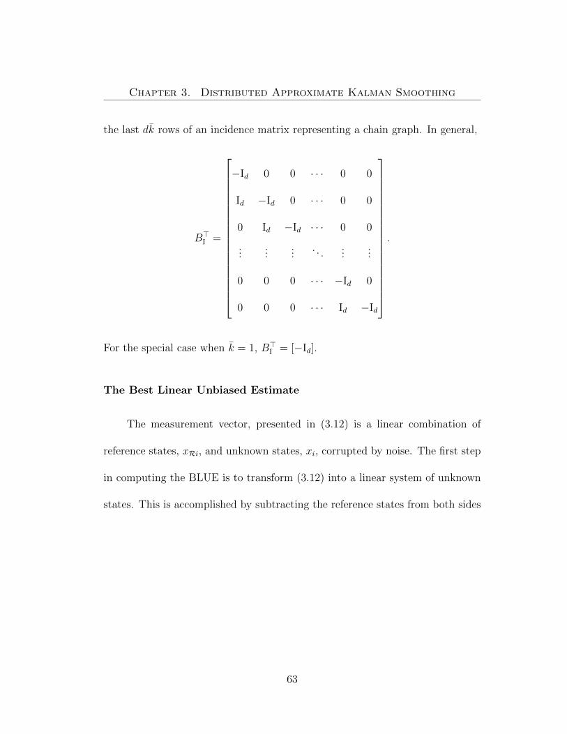
Chapter 3. Distributed Approximate Kalman Smoothing
the last dk rows of an incidence matrix representing a chain graph. In general,
B>I =
−Id 0 0 · · · 0 0
Id −Id 0 · · · 0 0
0 Id −Id · · · 0 0
......
.... . .
......
0 0 0 · · · −Id 0
0 0 0 · · · Id −Id
.
For the special case when k = 1, B>I = [−Id].
The Best Linear Unbiased Estimate
The measurement vector, presented in (3.12) is a linear combination of
reference states, xRi, and unknown states, xi, corrupted by noise. The first step
in computing the BLUE is to transform (3.12) into a linear system of unknown
states. This is accomplished by subtracting the reference states from both sides
63

Chapter 3. Distributed Approximate Kalman Smoothing
of the measurement equation
u1
y12
u2
y23
...
yη η−1
uη
−
e1 0 · · · 0
0 0 · · · 0
0 e1 · · · 0
0 0 · · · 0
......
. . ....
0 0 · · · 0
0 0 · · · e1
xR1
xR2
...
xRη
=
B>I 0 · · · 0
−Idk Idk · · · 0
0 B>I · · · 0
0 −Idk · · · 0
......
. . ....
0 0 · · · Idk
0 0 · · · B>I
x1
x2
...
xη
+
w1
v12
w2
v23
...
vη η−1
wη
.
(3.13)
To simplify this equation the following is introduced
z =
[u>1 y>12 u>2 y>23 . . . y>η η−1 u>η
]>,
xR =
[x>R1e
>1 0 x>R2e
>1 0 · · · x>Rηe
>1
]>,
B =
BI −Idk 0 0 · · · 0 0
0 Idk BI −Idk · · · 0 0
......
......
. . ....
...
0 0 0 0 · · · Idk BI
,
x =
[x>1 x>2 · · · x>η
]>,
64

Chapter 3. Distributed Approximate Kalman Smoothing
ε =
[w>1 v>12 w>2 v>23 . . . v>η η−1 wη
]>,
P =
Q1 0 0 0 · · · 0 0
0 R12 0 0 · · · 0 0
0 0 Q2 0 · · · 0 0
0 0 0 R23 · · · 0 0
......
......
. . ....
...
0 0 0 0 · · · Rη−1 η 0
0 0 0 0 · · · 0 Qη
.
Now, (3.13) can be written
z− xR = B>x + ε.
The BLUE, x∗, of x is defined to be
x∗ ≡ (BP−1B>)−1BP−1(z− xR). (3.14)
The Block-Jacobi Iterative Method
The algorithms presented in this chapter use the block-Jacobi iterative
method (introduced in section 3.2) to compute the BLUE. Now the the block-
65

Chapter 3. Distributed Approximate Kalman Smoothing
Jacobi method as it applies to computing (3.14) is examined. The BLUE, x∗,
is the unique solution to the linear equation Lx = b. To implement the block-
Jacobi method the matrix L = D − A is split so that D contains the block
diagonal elements of L. Then Ax is added to both sides of the linear equation
to form an estimate update law in accordance with the block-Jacobi method:
x(τ + 1) = D−1Ax(τ) +D−1b. (3.15)
Note that the update law is simply a discrete-time linear system. As such,
convergence is determined solely by the eigenvalues of D−1A.
To simplify further discussions, let the network iteration matrix be defined
as
J ≡ D−1A.
Denote by ρ(J) the magnitude of the largest eigenvalue of J – commonly known
as the spectral radius of J . Because J characterizes the dynamics of the Jacobi
Algorithm, a discrete-time linear system, convergence of the algorithm is depen-
dent on ρ(J). It was shown in Theorem 2 that for this problem, the block-Jacobi
method converges. Now it is shown to converge to the BLUE.
66

Chapter 3. Distributed Approximate Kalman Smoothing
Theorem 3 [Convergence to the BLUE]
Given that the block-Jacobi iteration in (3.15) converges,
limτ→∞
x(τ) = x∗.
Proof: When (3.15) is convergent,
x(∞) = D−1Ax(∞) +D−1b.
From this
x(∞) =(D − A)−1b
=(BP−1B>)−1BP−1(z− xR) = x∗.
Theorem 4 [Rate of Convergence for Scalar Covariance Matrices]
If the covariances, P{·}, for all measurements in the network are equal, then
ρ(J) ≤ 2
4− 2cos( π2k+1
).
67

Chapter 3. Distributed Approximate Kalman Smoothing
Proof: If all measurements have scalar covariance matrix, Ps = αI for α ∈ R,
the iteration matrix J can be written as
J =
0 Je 0 · · · 0 0 0
Jc 0 Jc · · · 0 0 0
0 Jc 0 · · · 0 0 0
......
......
......
0 0 0 · · · 0 Jc 0
0 0 0 · · · Jc 0 Jc
0 0 0 · · · 0 Je 0
,
where
Je =(BIP−1s B>I + P−1
s )−1P−1s
=(BIB>I + I)−1
Jc =(BIP−1s B>I + 2P−1
s )−1P−1s
=(BIB>I + 2I)−1.
From [16], for at least one block row, i, each eigenvalue of J , λk(J), satisfies
(‖ (Ji,i − λk(J)I)−1 ‖p
)−1 ≤∑i′ 6=i
‖Ji,i′‖p. (3.16)
68

Chapter 3. Distributed Approximate Kalman Smoothing
Being that all of the diagonal blocks, Ji,i are zero,
(‖ (Ji,i − λk(J)I)−1 ‖p
)−1= ‖λk(J)I‖p,
and (3.16) reduces to
‖λk(J)I‖p ≤∑i′ 6=i
‖Ji,i′‖p.
Using the 2-norm in the previous inequality and taking the maximum sum over
block rows,
ρ(J) ≤∑i′ 6=i
‖Ji,i′‖2 = maxi
∑i′ 6=i
ρ(Ji,i′). (3.17)
Equality in (3.17) comes from the fact that ‖Ji,i′‖ is symmetric.
Careful inspection reveals that
BIB>I =
2 −1 0 · · · 0 0
−1 2 −1 · · · 0 0
0 −1 2 · · · 0 0
......
.... . .
......
0 0 0 · · · 2 −1
0 0 0 · · · −1 1
.
69

Chapter 3. Distributed Approximate Kalman Smoothing
It was shown in [48], that the eigenvalues of BIB>I are λm = 2− 2cos
((2m−1)π
2τ+1
)for m ∈ {1, 2, . . . , τ}. Hence the eigenvalues of (BIB
>I + I) are λm = 3 −
2cos(
(2m−1)π2τ+1
)for m ∈ {1, 2, . . . , τ}. The smallest eigenvalue of (BIB
>I + I) is
the inverse of the spectral radius of JeP−1s , denoted ρe = 1
3−2cos( π2τ+1)
. In a similar
manner, it can be shown that the spectral radius of JcP−1s is ρc = 1
4−2cos( π2τ+1)
.
Each block row of J features either one JcP−1s block or two JeP
−1s blocks.
By inspection, ρe < 2ρc, hence ρ(J) ≤ 24−2cos( π
2τ+1).
There are a few things to note about this bound. First, the bound gets
tighter as η gets large. Second, the bound is independent of the number of
agents. Last, because 24−2cos( π
2τ+1)< 1, the Jacobi algorithm always converges.
Last, it is independent of the number of agents.
To illustrate the tightness of the bound, the following table shows the error
of the upper bound for several values of τ and η.
Table 3.1: Error of Upper Bounds Computed for ρ(J)τ
1 2 3 4
η
2 0 0 0 03 .0893 .0601 .0384 .02574 .0591 .0399 .0256 .01715 .0431 .0295 .0190 .0128
70

Chapter 3. Distributed Approximate Kalman Smoothing
3.5.2 Trade-off of Computation and Communication
Section 3.3.2 discussed how the MAI algorithm can be used to estimate the
state of distributed dynamic systems. There are two main parameters affecting
the performance of this algorithm, the amount of history retained for estimation,
κ, and the number of iterations at each time step, τ . Here, performance refers
to the covariance of estimate error. Higher performance relates to lower error
covariance (i.e. estimates that are ”tighter” to the optimal estimates). Both κ
and τ are positively correlated with performance; making these two values larger
improves performance.
The first parameter, κ, is the amount of history considered when perform-
ing distributed estimation. When κ is finite it is no longer possible to obtain
the global BLUE (the estimate that considers every measurement the network
has ever produced). This is due fixing the oldest estimates in the network. As
a set of nodes become the oldest nodes in the graph, they are deemed to be
reference nodes and their corresponding position estimates are taken as truth.
By doing this, whatever error remains in the estimates is fixed forever. It will be
demonstrated that even for κ relatively small, the method produces estimates
that are near optimal and generally much better than dead reckoning. Further-
more, increasing κ produces diminishing returns. When increasing κ by a fixed
amount, there is a larger performance increase when κ is small.
71

Chapter 3. Distributed Approximate Kalman Smoothing
As an iterative algorithm, if the MAI algorithm is convergent then each
iteration reduces the estimate error. As the number of iterations grows, the
estimates converge asymptotically to the BLUE. As such, increasing τ will im-
prove the estimate’s performance. As with κ, this effect has diminishing returns.
When increasing τ by a fixed amount, there is a larger performance increase
when τ is small. Also like κ, τ is limited by constraints within the network.
There is a finite limit to the number of iterations that are possible (i.e. much
information can be shared) in a single time step. The density of the network
and the bandwidth of the network’s communication channels greatly affect how
much information can be shared at each time step.
A logical question to ask when implementing the MAI algorithm on a dy-
namic system is just how well the algorithm will perform. This is not an easy
question to answer as it depends not only on κ and τ , but on the network’s
topology and the measurement and model fidelities as well. A lower bound for
the estimate error covariance is the estimate error covariance of the BLUE. Note
that the BLUE is equivalent to the estimate one obtains from the MAI algorithm
if κ =∞ and τ =∞. One can bound upper bound the estimate error covariance
with the covariance of dead-reckoning. For a given agent, the worst case scenario
would be for each agent to estimate their positions solely from inertial measure-
ments. Under the assumption that the inertial measurements have independent
72

Chapter 3. Distributed Approximate Kalman Smoothing
error, one would determine an agent’s current estimate error covariance by sum-
ming the covariances of inertial measurements from the agent’s reference node
to it’s current node. Note that dead reckoning is equivalent to a MAI algorithm
where τ = 0. In [5] Barooah and Hespanha showed that adding a measurement
to the network where there was not one previously can only reduce the error co-
variance of the BLUE. That is to say, by including inter-agent measurements in
the estimation scheme can only serve to improve the resulting position estimates.
Due to the topological dependence of the MAI algorithm, no general closed
form solution for the estimate covariance can be provided. However, given a spe-
cific network it is possible to explicitly compute the estimate error covariances.
To illustrate the utility of the MAI algorithm and also the trade-off between κ
and τ , covariance results that were calculated for the scenario where 10 agents
are moving together are presented. Initially, each agent knows it’s position ex-
actly. As the agents move along, they make relative position measurements to
their nearest neighbors. As shown in Figure 3.4, the measurements graph evolves
as a rectangular grid. The agents measurements (both inertial and inter-agent)
are corrupted with error of unity covariance.
Figure 3.5 shows the trade-off between κ and τ . This figure depicts the
agents’ average error covariance norm of current position estimates after 50 time
steps. With only one iteration per time step and only keeping two time steps in
73

Chapter 3. Distributed Approximate Kalman Smoothing
Figure 3.5: Average of the norm of agents’ real time estimate errors at k = 50.These estimates use only past measurements. The level sets show the trade-offsfor different values of κ and τ .
memory (the minimal parameters for the MAI algorithm to function), the agents’
average error covariance norm is 5.86. For comparison, in an uncooperative
environment (i.e. agents estimate positions using dead reckoning) the average
error covariance norm would by 50. The same metric for BLUE estimation (i.e. a
Kalman filter) is 5.55. Under very minimal assumptions, the algorithm provides
estimates with performance close to that of Kalman filtering. If the algorithm
parameters are increased so that κ = 5 and τ = 5, then the average error
covariance norm shrinks to 5.59 a mere 0.7% higher than the that of Kalman
filtering. Computationally, with these parameters the worst case is that an agent
must solve 5 optimizations with 12 equations and 4 unknowns at each time step.
74

Chapter 3. Distributed Approximate Kalman Smoothing
Figure 3.6 shows how the MAI algorithm performs as a smoother. This
figure shows the agents’ average error covariance norm for estimates at k = 40
using information gathered upto k = 50. These estimates approximate a fixed
interval smoother. With only one iteration per time step and only keeping two
time steps in memory, the agents’ average error covariance norm is 4.85. For
comparison, in an uncooperative environment the average error covariance norm
would by 40. The same metric for BLUE estimation is 4.33. If the algorithm
parameters are increased so that κ = 5 and τ = 5, then the average error
covariance norm shrinks to 4.40 a mere 1.5% higher than the that of Kalman
smoothing. Although these plots are for a particular scenario, the utility of
Figure 3.6: Average of the norm of agents’ smoothed estimate errors at k = 40.These estimates use a window of measurements, both past and present to improveestimate performance. The level sets show the trade-offs for different values ofκ and τ .
75

Chapter 3. Distributed Approximate Kalman Smoothing
the MAI algorithm is apparent. Under very reasonable conditions, the method
performs quite well.
3.6 Simulations
The MAI algorithm’s performance is further illustrated by numerical simu-
lations. All simulation results are shown for the case κ = 1. Five agents move in
a zig-zag trajectory; the resulting measurement graph is shown in Figure 3.7(a).
A time trace of the number of neighbors of Agent 1 is shown in Figure 3.7(b).
The initial position of Agent 1 (bottom left node in Figure 3.7) is taken as the
reference. Every measurement of xu − xv is obtained from noisy measurements
of the distance ‖xu−xv‖ and the angle between xu and xv. The distance and an-
gle measurements are corrupted with additive Gaussian noise, with σr = 0.05m
and σθ = 5o. The measurement error covariances are estimated from the range
and bearing measurements and the parameters σr, σθ (as explained in [4]), which
makes the covariances of the errors on relative position measurements on distinct
edges distinct.
Covariances of agent position estimates produced by the MAI algorithm are
estimated from 1000 Monte-Carlo runs. Figure 3.8 shows the covariance of the
estimate of x5(k), the position of Agent 5, as a function of k. Agent 5 is the
76
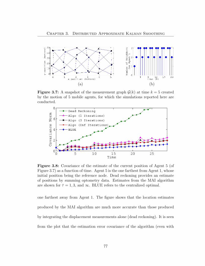
Chapter 3. Distributed Approximate Kalman Smoothing
(a) (b)
Figure 3.7: A snapshot of the measurement graph G(k) at time k = 5 createdby the motion of 5 mobile agents, for which the simulations reported here areconducted.
Figure 3.8: Covariance of the estimate of the current position of Agent 5 (ofFigure 3.7) as a function of time. Agent 5 is the one farthest from Agent 1, whoseinitial position being the reference node. Dead reckoning provides an estimateof positions by summing optometry data. Estimates from the MAI algorithmare shown for τ = 1, 3, and ∞. BLUE refers to the centralized optimal.
one farthest away from Agent 1. The figure shows that the location estimates
produced by the MAI algorithm are much more accurate than those produced
by integrating the displacement measurements alone (dead reckoning). It is seen
from the plot that the estimation error covariance of the algorithm (even with
77

Chapter 3. Distributed Approximate Kalman Smoothing
Figure 3.9: Covariance of the estimate of the current position of Agent 4 (ofFigure 3.7) as a function of time.
κ = 1 and τ = 1) is close to that of the centralized optimal estimator (BLUE).
Comparison among the plots for τ = 1, 3 and ∞ shows that, as expected, the
estimation accuracy improves with increasing number of iterations between every
time step. However, it is also seen that the improvement levels off quickly. In
fact, even with the minimal possible number of iterations τ = 1, the estimation
accuracy is quite close to the best possible (with τ = ∞). This property of the
algorithm enhances its applicability since good estimates are obtained with little
delay. Figure 3.9 plots these variables for the second agent.
78

Chapter 3. Distributed Approximate Kalman Smoothing
3.7 Conclusion
This chapter presented a distributed algorithm for mobile agents to esti-
mate their positions by fusing their own displacement measurements with inter-
agent relative position measurements. The algorithm is distributed in the sense
each agent can estimate its own position by communicating with nearby agents.
The algorithm computes an approximation of the centralized optimal (Kalman
smoother) estimates. The problem of distributed Kalman smoothing for this
application is reformulated as a problem of computing the BLUE estimates.
The graph structure of the BLUE estimation problem, opening the door for
distributed estimation algorithms. With finite memory and limited number of
iterations before new measurements are obtained, the algorithm produces an ap-
proximation of the Kalman smoother estimates. As the memory of each agent
and the number of iterations between each time step are increased, the approx-
imation improves.
This method was extended to include more general partitioning of the
graph’s node set. It was shown that by using a more general partitioning, the dis-
tributed estimation method can be extended to target tracking under a modest
observability assumption. A closed form bound for convergence of the algorithm
on a lattice with no constraint on memory was presented. Also, the trade off
79
Chapter 3. Distributed Approximate Kalman Smoothing
between the number of iterations per time step and the amount of history re-
tained during estimation was illustrated. It was shown that under very modest
parameters, the algorithm vastly improves estimates when compared to dead
reckoning. Furthermore, if the algorithm parameters are slightly improved per-
formance of the algorithm nears that of Kalman Smoothing. Finally, simulations
that illustrate the algorithm’s performance under very restrictive conditions were
presented. With a memory encompassing a single point in history, the algorithm
greatly outperforms dead-reckoning.
80

Chapter 4
Optimal Estimation on theGraph Cycle Space
This chapter proposes a solution to the distributed estimation from relative
measurements problem discussed in Chapter 2 and original explored in [4, 26, 37].
The relative difference measurement problem assumes that each sensor node (or
agent) in a network has an associated state that cannot be measured absolutely
(e.g. an agent’s global position), but a agent can measure the relative difference
between its state and its neighbor’s states (e.g. an agent can measure the range
and bearing to its neighbors). Barooah et al. explored several distributed al-
gorithms for this problem that converge to the optimal minimum error variance
solution [4]. Barooah’s algorithms assume that agents have limited topological
knowledge and communication abilities. In these algorithms, each agent com-
putes an estimate of its own state synchronously using an affine transformation
of neighboring state estimates. Methods that estimate the agent state directly
81

Chapter 4. Optimal Estimation on the Graph Cycle Space
are referred to as node estimation methods. The node estimation methods in-
troduced in [4] were shown to converge to the optimal estimate and were shown
to be robust to interruptions in communication.
The work reported in the present chapter is motivated by the observation
that, in the absence of noise, the sum of the relative difference measurements
around any cycle of the graph should be zero. However, due to measurement
noise, these sums are generally not equal to zero — these sums are referred to as
discrepancies. This naturally leads to the desire to find estimates with no dis-
crepancy that will sum to zero around the cycles of the graph. The graph cycle
space has been used in the past to solve several problems. Notably, Kirchoff pro-
posed that the redundancies present in cycles of electrical circuits could be used
to determine voltages within the circuits [22]. More recently, in [41], Rockafellar
discusses many properties of graph cycles and shows how the cycle space can be
used to determine flows in a network. Piovan et al. explored the use of cycles in
orientation localization from relative angle-of-arrival measurements in [38].
The Cycle Space Estimation algorithms introduced in this chapter consist
of two steps: first, one computes a “corrected” version of the measurement set
that has zero discrepancy and then one uses this corrected measurement set to
estimate the state variables. The first step can be done either in a centralized or
distributed fashion. Its decentralized version utilizes a Jacobi-like algorithm [35]
82

Chapter 4. Optimal Estimation on the Graph Cycle Space
on a “cycles graph” whose nodes correspond to the cycles of the original graph.
The second step can also be done in a centralized or distributed fashion. In the
latter case, convergence is guaranteed within a finite number of steps (equal to
the graph diameter) using the so-called flagged initialization algorithm [4].
For triangular, square, and hexagonal lattice graphs and certain classes
of random graphs, the new distributed algorithms converge significantly faster
than previous algorithms [4]. Our results show that, for large graphs, the Cycle
Space Estimation algorithm provides significant gains in terms of the number of
messages that are required to compute optimal estimates. This happens because
the cycles graph often has much better convergence properties than the original
graph. Monte Carlo simulations are used to show that this is the case for several
classes of regular graphs, which include square, triangular, and hexagonal lattices
of varying size. For square lattices, there are also explicit formulas to compute
the convergence rate of the distributed algorithm.
This chapter expands upon results previously presented in [44]. Specifically,
this chapter presents new convergence results for the distributed algorithm pre-
sented herein as well as expanded simulation results comparing this method to
a preexisting distributed estimation algorithm.
This chapter proceeds in the following manner. In Section 4.1, the Cen-
tralized Optimal Cycle Space Estimate is introduced. The Distributed Optimal
83

Chapter 4. Optimal Estimation on the Graph Cycle Space
Cycle Space Estimation algorithm is covered in Section 4.2. The convergence
properties of the Distributed Optimal Cycle Space Estimation algorithm are dis-
cussed in Section 4.3. Simulation results are given in Section 4.4. Conclusions
and future research goals are discussed in Section 4.5.
4.1 Centralized Cycle Space Estimation
To gain insight into the approach followed here, it is convenient to regard
the states of the agents as voltages in an electric circuit that takes the shape of
the measurement graph. The measurements would then correspond to tensions
measured across the edges of the graph. When the graph has cycles, one should
obtain zero by summing the tensions along a cycle (a la Kirchhoff’s Voltage
Law), but because of measurement errors this is generally not the case. In this
light, one can view the estimation procedure as computing a set of voltages that
are internally consistent, in the sense that they add up to zero around any cycle
(i.e. the set satisfies KVL).
Let us define the optimal tension estimate vector as:
z∗ ≡[BTR B
T
]xR
x∗
, (4.1)
84

Chapter 4. Optimal Estimation on the Graph Cycle Space
where x∗ is the minimum variance estimate for x from (3.14). The vector z∗
defined above is obtained by taking differences between all elements of the op-
timal estimate x∗ for which there are measurements available. That is, z∗ is the
optimal estimate of differences in x. In the absence of noise, x∗ would be equal
to x and z∗ would be equal to the measurement vector, z, which in turn is equal
to the non-noisy state differences, BTx.
While it appears from (4.1) that one needs to first compute the optimal
estimate x∗ to compute the optimal tension estimate z∗, it will be demonstrated
shortly that it is possible to compute z∗ directly from the measurements z, and
that it is then straightforward to obtain x∗ from z∗. It will also be shown that
this indirect procedure can be advantageous from the perspective of reducing
communication and computation when implemented as a distributed algorithm.
The remainder of this section is split into three parts. The first subsection
introduces the cycle space of a graph. The next subsection details how the
centralized optimal tension estimate is computed. The last subsection provides
a method for computing the BLUE from the optimal tension estimate.
4.1.1 Cycle Space
A simple cycle of G is a sequence of alternating nodes and edges that starts
and ends at the same node and has only this one repeated node. The direction
85

Chapter 4. Optimal Estimation on the Graph Cycle Space
of a cycle is given innately by the order in which the nodes of the cycle are
visited. A simple cycle need not follow the direction of its edges; a cycle may
traverse an edge forward or backward. By indexing the edges with the natural
from numbers 1 to m, a simple cycle vector can be assigned to each simple cycle,
which is defined to be the m-length vector c = (c1, . . . , cm)T, where,
cj ≡
1 if cycle traverses edge j forward
−1 if cycle traverses edge j backward
0 otherwise.
The cycle space, C, of G is then defined to be the subspace of Rm generated by
the simple cycle vectors associated with the simple cycles in G. Subsequently,
C will be used to denote the Kronecker product of a matrix whose columns are
simple cycle vectors that form a basis for the cycle space and the identity matrix
of size d, the dimension of the measurements. Considering that every column of
BG corresponds to an edge in G, C is a basis for the nullspace of BG [41]. The
cycle space matrix, C, has height dm and width dr, where r is the dimension of
C. For an example cycle space matrix, see Figure 4.1.
86

Chapter 4. Optimal Estimation on the Graph Cycle Space
C =
[1 −1 1 −1 0 00 1 0 0 1 −1
]T
Figure 4.1: An example graph shown along with a cycle space matrix, C. Notethat c3 = c1 + c2 is a cycle that is not in the basis, C.
4.1.2 The Centralized Optimal Tension Estimate
Optimal tension estimation uses z and C to compute z∗. The premise of
optimal tension estimation is that one can add a correction term to the mea-
surement vector, z, to form the optimal tension estimate vector, z∗. This idea is
formalized in the following result, which is a main contribution in this work.
87

Chapter 4. Optimal Estimation on the Graph Cycle Space
Theorem 5 [The Optimal Tension Estimate]
The optimal tension estimate from (4.1),
z∗ =
[BTR BT
]xRx∗
,
is the solution to the quadratic programming problem:
z∗ = argminz
[(z− z)TP−1(z− z)] s.t. CTz = 0 (4.2)
=
z− PC(CTPC)−1CTz if r 6= 0
z if r = 0.
(4.3)
Proof: When r = 0 (G has no cycles), CT is trivial and the constraint in
(4.2) is satisfied for any z. Consequentially, z∗ = z. Furthermore, with no
cycles in the graph, the BLUE of a particular agent is simply the summation
of measurements along the unique path from the reference agent to the agent
in question. As such, the difference in the BLUEs of two neighboring agents is
simply the measurement connecting these agents. Hence, the optimal tension
vector for which (4.1) holds is the measurement vector, z.
88

Chapter 4. Optimal Estimation on the Graph Cycle Space
When r 6= 0, the Lagrangian for (4.2) is:
L(z,Λ) = (z− z)TP−1(z− z) + ΛTCTz.
Taking the partial derivatives of the Lagrangian equal to zero:
∂L
∂z= 2P−1(z− z) + CΛ = 0
∂L
∂Λ= CTz = 0,
which can be written in the form:
2P−1 C
CT 0
z
Λ
=
2P−1z
0
. (4.4)
Using the Schur Complement (see [28]), (4.4) can be solved to find z∗:
z∗ =
[12P − 1
2PC(CTPC)−1CTP
]2P−1z
= [I − PC(CTPC)−1CT]z. (4.5)
Lemma 2 (in the Appendix) is used to show that (4.5) is related to the BLUE
by (4.1). Lemma 2 states that for two full column rank matrices, α and βT, the
89

Chapter 4. Optimal Estimation on the Graph Cycle Space
image of α is the nullspace of β if and only if
α(αTα)−1αT = I − βT(ββT)−1β.
Consider the matrices β = image(BP−12 ) and α = image(P
12C). Note that
null(β) = image(α). Considering Lemma 2 and the fact that CTBTR = 0, the
following equalities hold:
0 = [α(αTα)−1CTP12 ]P−
12BTRxR
= [α(αTα)−1αT]P−12BTRxR
= [I − βT(ββT)−1β]P−12BTRxR
= P12 [I − βT(ββT)−1β]P−
12BTRxR
= [I − P12βT(ββT)−1βP−
12 ]BT
RxR
= [I −BT(BP−1BT)−1BP−1]BTRxR. (4.6)
90

Chapter 4. Optimal Estimation on the Graph Cycle Space
Consider again Lemma 2:
I − α(αTα)−1αT = βT(ββT)−1β
I − P12α(αTα)−1αTP−
12 = P
12βT(ββT)−1βP−
12
I − PC(CTPC)−1CT = BT(BP−1BT)−1BP−1
[I − PC(CTPC)−1CT]z = BT(BP−1BT)−1BP−1z. (4.7)
Now, add (4.6) to (4.7):
[I − PC(CTPC)−1CT]z =BT(BP−1BT)−1BP−1z
+ [I −BT(BP−1BT)−1BP−1]BTRxR
=BTRxR +BT(BP−1BT)−1BP−1(z−BT
RxR)
=BTRxR +BTx∗ ≡ z∗.
In light of Theorem 5 the following interpretation of z∗ can be made: The
tension vector corresponding to the BLUE, x∗, is the tensions vector with the
least square difference from the measurement vector, z. That is to say, it is the
tension vector with minimum squared edge modification.
91

Chapter 4. Optimal Estimation on the Graph Cycle Space
4.1.3 The Centralized Optimal State Estimate
As expressed in (4.1), the optimal tension estimate, z∗, is a vector of the
relative difference in BLUEs, x∗. Because the optimal tension estimates are
consistent (i.e. they sum to zero around cycles), the sum of optimal tension
estimates between any two points in the graph is path independent. As such,
the optimal estimate of any agent’s state can be found by summing the optimal
tension estimates along a path from a reference agent to the agent.
To represent a path between Agent i and Agent i′, define a path vector to
be the m-length row-vector hi,i′ = (h1, . . . , hm)T, where,
hj ≡
1 if the path traverses edge j forward
−1 if the path traverses edge j backward
0 otherwise.
Let T ∈ G be the subgraph corresponding a minimal spanning forest that consists
of trees rooted at the nodes corresponding to reference agents. That is, T is a
graph where all nodes are weakly connected (i.e. connected without respect to
edge direction) to the reference node and the number of edges in the graph is
minimized [50]. The path vector matrix of graph T is then defined to be an n by
92

Chapter 4. Optimal Estimation on the Graph Cycle Space
m matrix where the ith row is a path vector from the reference agent to Agent i:
HT ≡
h1,R
...
hn,R
.
Finally, x∗ can be computed from z∗ using,
x∗ =
xR
...
xR
+HT z∗.
The preceding equation relates that the optimal estimate of an agent’s state is
simply the state of the reference agent plus the sum of optimal tension estimates
along a path connecting the agent to the reference agent.
4.2 Distributed Cycle Space Estimation
In a large network it is often impractical to collect all of the measurements
at one agent, compute the optimal estimate at that agent, and then redistribute
the estimate to every other agent. Instead, it is desirable to find an estimate of
the state in a distributed manner.
93

Chapter 4. Optimal Estimation on the Graph Cycle Space
This section presents the Jacobi Cycle Space Estimation (JCSE) algorithm,
a distributed algorithm that uses the cycles of the graph to solve the estimation
from relative measurements problem. JCSE uses two levels of computation in
series to estimate the graph states, x. The first level in the JCSE algorithm
iteratively computes a tension estimate, zj, for all edges of the graph, ej ∈ E .
The second level in the JCSE algorithm uses the tension estimates from the first
level to compute state estimates, xi, for all nodes in the graph, vi ∈ V .
In the first level of the JCSE algorithm, each edge, ej, has associated with
it a tension estimate, zj, that is initialized zj, the measurement corresponding
to the edge j. Also, each simple cycle, ck ∈ C, has a d-length vector iteration
variable, yk. At each iteration yk is computed to be the value that, when added
to the tension estimates of edges in ck, will make these tension estimates consis-
tent. An edge may exist in multiple cycles (causing the cycles to be adjacent)
and these cycles generally will not agree on what value must be added to the
respective measurement to make it consistent. Because of this, the cycles iter-
atively refine their iteration variables to account for adjacent cycles’ iteration
variables. While this iteration is proceeding, the tension estimate for an edge
is continually recomputed to be a weighted sum of iteration variables for cycles
that the edge is a part of added to the measurement associated with the the
edge.
94

Chapter 4. Optimal Estimation on the Graph Cycle Space
The second level of the JCSE algorithm uses the tension estimates, zj, to
compute state estimates, xi. This comes about naturally because zj are estimates
of differences in two states. As such, if the tension estimates along a path from
a node, vi, to any reference node are available, then the sum of these tension
estimates provides xi, the estimate of the state of vi.
To improve readability, the remainder of this section is divided into three
parts. First several structures including the weighted cycle degree matrix, the
weight cycle adjacency matrix, and the cycle Laplacian are defined. Of these
matrices, the first two are used in the JCSE algorithm and the last is used to
illustrate how the first two matrices relate to the cycle space matrix, C. The
second subsection presents a distributed tension estimation algorithm. The last
subsection presents a distributed algorithm that estimates the agent states from
the distributed tension estimates.
4.2.1 Cycle Laplacian
Motivated by (4.3) cycle Laplacian matrix is defined as,
Lc ≡ CTPC. (4.8)
95

Chapter 4. Optimal Estimation on the Graph Cycle Space
While Lc is generally not doubly stochastic, it is called the Laplacian because it
characterizes the weighted cycle degree and the weighted cycle adjacency, which
are defined as follows: let Bk ⊂ E be the set of edges in ck ∈ C, the cycle
corresponding to the kth column of the cycle space basis matrix C. Define the
weighted cycle degree matrix, Dk, of this cycle as the sum of the error covariance
matrices, Pj as defined in (2.4), of measurements corresponding to edges j ∈ Bk,
i.e.
Dk ≡∑j∈Bk
Pj.
Define the weighted cycle adjacency matrix, Ak,k′ between two cycles, ck and c′k,
as the net sum of error covariance matrices, Pj, corresponding to measurements
that exist in both cycles, i.e. j ∈ Bk ∩ Bk′ . The cycle adjacency between two
cycles increases if both cycles traverse the edge in the same direction and de-
creases if the cycles traverse the edge in opposite directions. The cycle adjacency
between ck and c′k is
Ak,k′ ≡∑
j∈Bk∩Bk′
Pjcj,kcj,k′ ,
where cj,k is the jth element of ck (the element in the jth row and kth column
of the cycle space matrix, C). If two cycles have no common edges, then the
weighted adjacency between the cycles is zero. The weighted cycle degree and
96

Chapter 4. Optimal Estimation on the Graph Cycle Space
weighted cycle adjacency, so defined, are related to the cycle Laplacian by
Lc = D − A,
D = diag(D1, . . . , DR),
A = [Ak,k′ ].
To solidify the idea of cycle degree, cycle adjacency, and cycle laplacian,
consider the example graph shown in Figure 4.1. If all measurements in the
graph have covariance, Pm, then,
D =
4Pm 0
0 3Pm
, A =
0 Pm
Pm 0
, Lc =
4Pm −Pm
−Pm 3Pm
.
4.2.2 The Distributed Tension Estimate
Formally, the following assumptions are made for the JCSE algorithm:
1. An agent knows the measurements corresponding its edges.
2. Each agent knows how to send messages to each one of its neighbors in G.
3. A basis C for the cycle space of the graph is known and a “leader” has
been elected for each simple cycle corresponding to the columns of C.
97

Chapter 4. Optimal Estimation on the Graph Cycle Space
4. All agents that belong to one (or more) of the simple cycles associated
with a column of C know how to send measurements to the leaders of
these cycles (perhaps through multi-hop communication).
JCSE starts with each cycle leader collecting the sum of measurements in
its cycle. Each cycle leader then computes the total discrepancy in its cycle by
adding the measurements of the cycle: ∆k =∑
j∈Bk zj. Note that all of the
discrepancies can be represented in one equation as ∆ = CTz.
Each cycle leader possesses an iteration variable yk that is initialized to
zero. Let Ak be the set of cycles that share at least one edge with cycle k. Then,
as the JCSE algorithm proceeds, at each step each cycle leader:
1. Sends the value of its iteration variable, yk, to the leaders of the cycles
that share edges with its own cycle, as well as to all the agents in its cycle,
2. Receives iteration variables, yAk from the leaders of neighboring cycles,
3. Recomputes its iteration variable,
yt+1k = D−1
k
(∑k′∈Ak
Ak,k′ ytk′ −∆k
). (4.9)
In addition to the iteration above carried out by the cycle leaders, each
agent also maintains internal estimates of tensions for all its incident edges. In
98

Chapter 4. Optimal Estimation on the Graph Cycle Space
particular, the estimate of the tension ztj for edge j is computed as follows:
ztj = zj + Pj∑k∈Kj
ytk, (4.10)
where zj is the measurement corresponding to the edge j, Pj the error covariance
for that edge, and Kj denotes the set of cycles that contain the edge j. The set
Kj can be empty if the edge does not belong to any cycle, in which case ztj = zj.
4.2.3 The Distributed State Estimate
To obtain its current state estimate from the tension estimates, an agent
needs only to obtain the sum of the tensions along a path between itself and a
reference agent, which can be accomplished via a distributed flagging method
similar to that introduced in [4]. In this way, all non-reference agents start
with a flagged state value, x0 = ∞. The first time that a node, say vi ∈ V ,
communicates with a neighbor, say vi′ ∈ V , that has a non-flagged state, vi
is aware that vi′ is the last node in a path connected to a reference node. vi
will then compute its state estimate, xt+1i , to be vi′ ’s state, xti′ , plus or minus
(depending on the orientation of the edge that connects the nodes, ei,i′ ∈ E) the
tension estimate connecting the two nodes, zti,i′ . As the state estimates, xt, and
tension estimates, zt, are refined, vi will maintain its estimate as the current
99
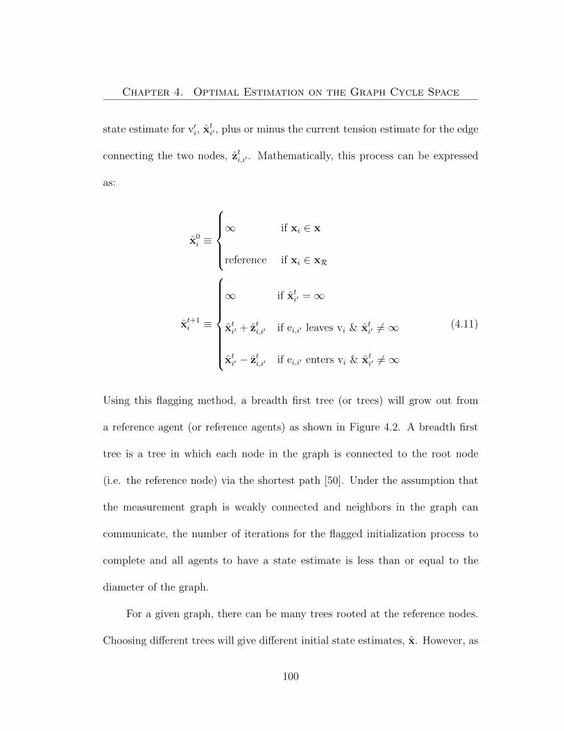
Chapter 4. Optimal Estimation on the Graph Cycle Space
state estimate for v′i, xti′ , plus or minus the current tension estimate for the edge
connecting the two nodes, zti,i′ . Mathematically, this process can be expressed
as:
x0i ≡
∞ if xi ∈ x
reference if xi ∈ xR
xt+1i ≡
∞ if xti′ =∞
xti′ + zti,i′ if ei,i′ leaves vi & xti′ 6=∞
xti′ − zti,i′ if ei,i′ enters vi & xti′ 6=∞
(4.11)
Using this flagging method, a breadth first tree (or trees) will grow out from
a reference agent (or reference agents) as shown in Figure 4.2. A breadth first
tree is a tree in which each node in the graph is connected to the root node
(i.e. the reference node) via the shortest path [50]. Under the assumption that
the measurement graph is weakly connected and neighbors in the graph can
communicate, the number of iterations for the flagged initialization process to
complete and all agents to have a state estimate is less than or equal to the
diameter of the graph.
For a given graph, there can be many trees rooted at the reference nodes.
Choosing different trees will give different initial state estimates, x. However, as
100

Chapter 4. Optimal Estimation on the Graph Cycle Space
Figure 4.2: An example of the breadth first flagging method. In the first timeinstant only the reference agent has an estimate of its state. At t = 1 bothof the reference agent’s neighbors have estimates of their states. By t = 2, allagents have state estimates and a breadth first tree has been created for thegraph (indicated by bold edges).
the tension estimates converge to the optimal estimate, z∗, the state estimates
obtained using any tree will converge to the minimum variance estimate, x∗,
because z∗ is consistent.
4.3 Convergence of the JCSE Algorithm
The convergence properties for the JCSE can be examined by considering
the algorithm’s effects on the graph as a whole. Start by stacking the iteration
variables, yk, into a single dr-length vector, y. The update law (4.9) can be
rewritten:
yt+1 = D−1(Ayt −∆
), (4.12)
where D is the graph’s weighted cycle degree matrix, A is the graph’s weighted
cycle adjacency matrix, and ∆ is the vector of cycle discrepancy. Similarly,
101

Chapter 4. Optimal Estimation on the Graph Cycle Space
when the tension estimates are stacked into a single vector, z, the update law
corresponding to (4.10) can be expressed as:
zt = z + PCyt. (4.13)
To represent the flagging process in a similar manner, define the directed adja-
cency matrix of graph G as AG = [aii′ ], i ∈ {1, . . . , n}, i′ ∈ {1, . . . , n},
aii′ ≡
Id if an edge leaves node i′ and enters node i
0 otherwise.
Define the in-incidence matrix of graph G as BinG =
[binij
], i ∈ {1, . . . , n}, j ∈
{1, . . . ,m},
binij ≡
−Id if edge j enters node i
0 otherwise.
As previously discussed, the flagging procedure in (4.11) constructs a breadth
first tree rooted at the reference node. Denote this tree as the subgraph T ∈ G,
then the flagging process can be represented using the equation:
χt+1 = ATχt +BT zt, (4.14)
102
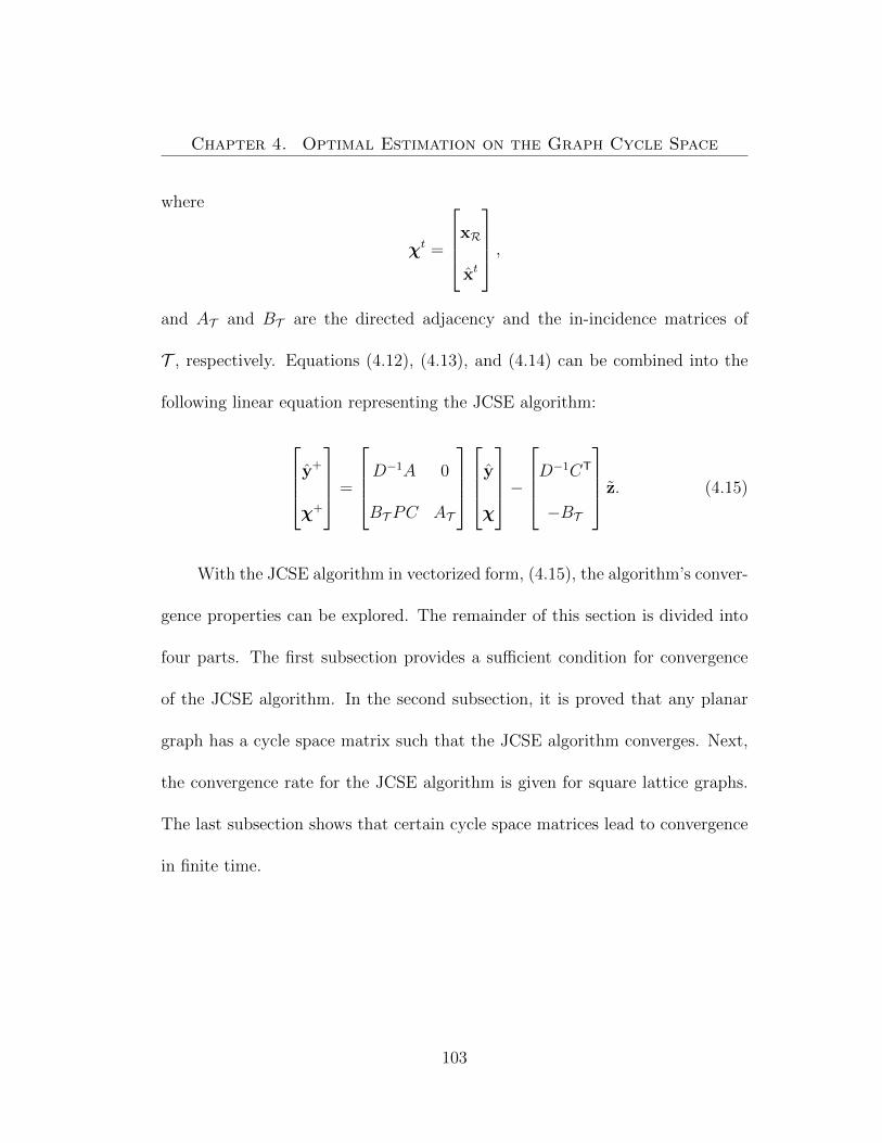
Chapter 4. Optimal Estimation on the Graph Cycle Space
where
χt =
xR
xt
,and AT and BT are the directed adjacency and the in-incidence matrices of
T , respectively. Equations (4.12), (4.13), and (4.14) can be combined into the
following linear equation representing the JCSE algorithm:
y+
χ+
=
D−1A 0
BT PC AT
y
χ
−D−1CT
−BT
z. (4.15)
With the JCSE algorithm in vectorized form, (4.15), the algorithm’s conver-
gence properties can be explored. The remainder of this section is divided into
four parts. The first subsection provides a sufficient condition for convergence
of the JCSE algorithm. In the second subsection, it is proved that any planar
graph has a cycle space matrix such that the JCSE algorithm converges. Next,
the convergence rate for the JCSE algorithm is given for square lattice graphs.
The last subsection shows that certain cycle space matrices lead to convergence
in finite time.
103

Chapter 4. Optimal Estimation on the Graph Cycle Space
4.3.1 Condition for Convergence of the JCSE Algorithm
The following theorem provides a sufficient condition for convergence of the
JCSE algorithm.
Theorem 6 [Sufficient Condition for Convergence]
Given D and A, the weighted cycle degree matrix and the weighted cycle ad-
jacency matrix, respectively, if the spectral radius (i.e. the largest eigenvalue)
of D−1A is strictly less than 1, then the JCSE algorithm converges, the tension
estimate, zt, converges to the optimal (weighted minimum mean squared error)
tension estimate, z∗, and the state estimate, x, converges to the BLUE, x∗.
Proof: In view of (4.15), the JCSE algorithm is a cascade linear system;
for stability, both sections of the cascade must be stable. All eigenvalues for
the adjacency matrix for the directed tree, AT , are zero. This can be seen by
enumerating nodes in the tree according to their proximity to reference nodes.
The reference nodes in the graph have the lowest number, followed by neighbors
of reference nodes, etc; the leafs on the tree are labeled with the the largest
numbers. When this is done, AT is strictly lower triangular and therefore has
only zero eigenvalues. From this, the rate of convergence for (4.15) is bounded
by the spectral radius, ρ(J), of the iteration matrix, J = D−1A.
104

Chapter 4. Optimal Estimation on the Graph Cycle Space
From (4.12), when yt converges, y∗ = D−1(Ay∗ −∆). The error between
yt and y∗ has the following dynamics:
yt+1 − y∗ = D−1(Ayt −∆)−D−1(Ay∗ −∆)
= D−1A(yt − y∗).
When the spectral radius of D−1A is strictly less than 1, the error between yt and
y∗ goes to zero as t goes to infinity. Similarly, from (4.13), when zt converges,
z∗ = z + PCy∗. The error between zt and z∗ has the following dynamics:
zt+1 − z∗ = z + PCyt − z + PCy∗
= PC(yt − y∗).
If the spectral radius of D−1A is less than 1 and yt − y∗ goes to zero as t goes
to infinity, then zt − z∗ will also go to zero as t goes to infinity. Furthermore,
105

Chapter 4. Optimal Estimation on the Graph Cycle Space
when yt converges:
y∗ = D−1(Ay∗ −∆)
Dy∗ = Ay∗ −∆
(D − A)y∗ = −∆
(CTPC)y∗ = −CTz
y∗ = −(CTPC)−1CTz,
from which, z∗ = z−PC(CTPC)−1CTz. Hence the tension estimate, z converges
to the optimal tension estimate, (4.3).
Theorem 5, tells us that the optimal tension estimate vector, z∗, consists of
the pairwise differences of the BLUE, xi∗, corresponding to edges in the graph.
As such, summing z∗ along the directed tree provided by AT and BT renders
the BLUE.
Because C is only required to be a basis for the cycle space, C is not unique.
Consequentially, the choice of C affects the behavior of the JCSE because A and
D depend on C. While Theorem 6 provides conditions for convergence based on
the spectral radius of D−1A, it does little to explain which cycle space matrices
lead to convergent cycle space estimates. The optimal choice of C remains an
106

Chapter 4. Optimal Estimation on the Graph Cycle Space
open problem; however, the following convergence results can be used to evaluate
potential C matrices.
4.3.2 Convergence of JCSE on a Planar Graph
When a planar graph is embedded in the Euclidean Plane such that no edges
cross, the plane is divided into contiguous regions called faces (see Figure 4.3 for
an example of graph faces); each graph face characterizes a cycle that forms its
boundary [21]. The faces of the graph are taken to be the set of interior faces in
the graph, which is a basis for the cycle space of the graph [24]. The following
theorem provides a convergence result for planar graphs. In this theorem, the
faces of the graph are chosen to derive the basis for the cycle space.
Figure 4.3: Simple graph with interior faces A,B,C, and D and exterior face E.
107

Chapter 4. Optimal Estimation on the Graph Cycle Space
Theorem 7 [Convergence for Planar Graphs]
When G is a planar graph and C is the basis of the cycle space associated with the
internal faces of the graph, then the JCSE, (4.15), converges and limt→∞ xt = x∗,
the BLUE of x.
Proof: The cycle degree matrix, D, is a block diagonal matrix whose blocks
are sums of covariance matrices. As such, D and D−1 are symmetric positive
definite matrices. The cycle Laplacian matrix is defined as Lc ≡ CTPC, where P
is symmetric positive definite and C is a basis, hence Lc is a symmetric positive
definite matrix. From [19] (Theorem 7.6.3) all eigenvalues of D−1Lc are positive,
from which:
ρ(D−1Lc
)> 0
ρ(I −D−1Lc
)< 1
ρ(I −D−1(D − A)
)< 1
ρ(D−1A
)< 1
Hence, the JCSE algorithm converges.
108
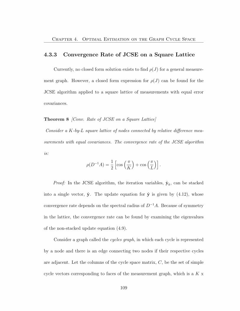
Chapter 4. Optimal Estimation on the Graph Cycle Space
4.3.3 Convergence Rate of JCSE on a Square Lattice
Currently, no closed form solution exists to find ρ(J) for a general measure-
ment graph. However, a closed form expression for ρ(J) can be found for the
JCSE algorithm applied to a square lattice of measurements with equal error
covariances.
Theorem 8 [Conv. Rate of JCSE on a Square Lattice]
Consider a K-by-L square lattice of nodes connected by relative difference mea-
surements with equal covariances. The convergence rate of the JCSE algorithm
is:
ρ(D−1A) =1
2
[cos( πK
)+ cos
(πL
)].
Proof: In the JCSE algorithm, the iteration variables, yk, can be stacked
into a single vector, y. The update equation for y is given by (4.12), whose
convergence rate depends on the spectral radius of D−1A. Because of symmetry
in the lattice, the convergence rate can be found by examining the eigenvalues
of the non-stacked update equation (4.9).
Consider a graph called the cycles graph, in which each cycle is represented
by a node and there is an edge connecting two nodes if their respective cycles
are adjacent. Let the columns of the cycle space matrix, C, be the set of simple
cycle vectors corresponding to faces of the measurement graph, which is a K x
109

Chapter 4. Optimal Estimation on the Graph Cycle Space
Figure 4.4: Example of the interconnection of cycles and iteration variables ina lattice graph.
L square lattice. The cycles graph is a (K − 1) x (L− 1) grid (see Figure 4.4).
Enumerate the faces of the graph based on their grid location in the faces graph.
Denote by yk,l the cycle iteration variable for the face in the kth row and lth
column of the cycles graph, where k ∈ {1, . . . , K − 1} and l ∈ {1, . . . , L − 1}.
Because all of the faces in a square lattice have four edges, the cycle degree for
each face is 4Pm, where Pm is the covariance matrix of a single measurement.
Furthermore, if two faces are adjacent, they share exactly one edge and have a
cycle adjacency of Pm. With a cycle degree of 4Pm and a cycle adjacency of Pm,
110

Chapter 4. Optimal Estimation on the Graph Cycle Space
the iteration variable update equation, (4.9), can be expressed as:
y+k,l =
1
4(yk+1,l + yk−1,l + yk,l+1 + yk,l−1)− 1
4P−1
m ∆k,l,
where y0,l = yK,l = yk,0 = yk,L = 0. In steady state:
y∗k,l =1
4(y∗k+1,l + y∗k−1,l + y∗k,l+1 + y∗k,l−1)− 1
4P−1
m ∆k,l.
The error between yk,l and y∗k,l, for k ∈ {1, . . . , K − 1} and l ∈ {1, . . . , L − 1},
evolves as:
e+k,l =
1
4(ek+1,l + ek−1,l + ek,l+1 + ek,l−1), (4.16)
where e0,l = eK,l = ek,0 = ek,L = 0. Equation (4.16) is a Discrete Poisson Equa-
tion with homogeneous Dirichlet boundary conditions. From [14] (Chapter 4,
Section 3.3), a Discrete Poisson Equation with homogeneous Dirichlet boundary
conditions has eigenfunctions of the form:
ek,l = sin
(πµk
K
)sin
(πνl
L
), (4.17)
111

Chapter 4. Optimal Estimation on the Graph Cycle Space
where µ ∈ {1, . . . , K − 1} and ν ∈ {1, . . . , L− 1}. Eigenvalues for (4.16), λ, can
be found by substituting in the eigenfunction, (4.17):
λek,l =1
4(ek+1,l + ek+1,l + ek,l+1 + ek,l−1),
as such:
λ
[sin
(πµk
K
)sin
(πνl
L
)]=
1
4
[sin
(πµ(k + 1)
K
)sin
(πνl
L
)+
sin
(πµ(k − 1)
K
)sin
(πνl
L
)+
sin
(πµk
K
)sin
(πν(l + 1)
L
)+
sin
(πµk
K
)sin
(πν(l − 1)
L
)]. (4.18)
Making use of the trigonometric identity, sin(a+b) = sin(a) cos(b)+cos(a) sin(b),
(4.18) reduces to:
λ
[sin
(πµk
K
)sin
(πνl
L
)]=
1
2
[sin
(πµk
K
)sin
(πνl
L
)cos(πµK
)+
sin
(πµk
K
)sin
(πνl
L
)cos(πνL
)],
112

Chapter 4. Optimal Estimation on the Graph Cycle Space
which simplifies further to:
λ =1
2
[cos(πµK
)+ cos
(πνL
)],
which is largest in magnitude when µ = 1 and ν = 1. Hence, the spectral radius
of linear system (4.16) is
λmax =1
2
[cos( πK
)+ cos
(πL
)].
4.3.4 Single Step Convergence
As defined, the entries of C are from the set {1, 0,−1}. The graphs cycles
have a physical representation; they are a collection of edges. If this constraint
on C is relaxed and the elements are allowed to be real numbers, the following
result is obtained.
Theorem 9 [Convergence in One Iteration]
If C is chosen to be a orthogonal basis, then the JCSE algorithm converges in a
single iteration.
113

Chapter 4. Optimal Estimation on the Graph Cycle Space
Proof: When C is chosen to be a orthogonal basis of the cycle space, the
cycle Laplacian matrix, Lc, is a block diagonal matrix, with blocks of size d, the
dimension of the measurements. Consequentially, all elements of cycle adjacency
matrix, A, and iteration matrix, J , are equal to zero. Hence, the cycle iteration
variables, yk, are set to the cycle discrepancy, ∆k, on the first iteration.
In general, when C is chosen to be a orthogonal basis for the cycle space,
the cycle Laplacian matrix, Lc, will not be sparse, indicating that cycle leaders
performing JCSE will need to collect and share information with many other
cycle leaders. While this is not a desirable trait in a distributed algorithm, it-
eration on this basis may render solutions with less communication than the
classic centralized solution (one in which all measurements are passed to a cen-
tral processor). This is because the cycle leaders only need to know the cycle
discrepancy (a weighted sum of measurements as opposed to the measurements
themselves).
For example, consider a ring graph with n nodes. Computing the sum
around the ring takes n messages. However, to pass all of the messages to one
node for processing would take n2−14
messages (for an odd number of nodes). This
can be seen by considering a graph with an odd number of nodes. The furthest
distance a measurement must travel is n−12
(there are two such measurements).
114

Chapter 4. Optimal Estimation on the Graph Cycle Space
The next furthest distance is n−12− 1, etc. Two times the sum from 1 to n−1
2is
n2−14
.
4.4 Simulations
The chief aim of this work is to develop a distributed estimation algorithm
that swiftly converges to the BLUE. As such, it is appropriate to offer a compar-
ison with previously developed algorithms. The Jacobi Algorithm introduced in
[4] is a node estimation method that uses relative state difference measurements
to compute the optimal estimate of a graph’s state. In the Jacobi Algorithm,
each agent considers a local subgraph consisting of itself, its one-hop neighbors,
and all edges incident on itself. At each iteration, each agent shares (with its
neighbors) its estimate of its own position. Each agent then computes the BLUE
(3.14) of its local subgraph assuming that its neighbors’ own estimates of state
are reference. The Jacobi Algorithm With Flagged Initialization (JAWFI) is
an improved version of the Jacobi algorithm where agents with unknown state
initialize their estimates to a flagged condition. When computing the BLUE of
its local subgraph, a agent only includes estimates of neighbors with non-flagged
state. Figure 4.5 compares the spectral radii of this node estimation method
and the JCSE algorithm (where the cycle space is chosen to be the faces of the
115

Chapter 4. Optimal Estimation on the Graph Cycle Space
graph). For triangular, square, and hexagonal lattices, the JCSE always has a
smaller spectral radius and therefore has a faster convergence rate.
0 5 10 15 20 250
0.25
0.5
0.75
1
Lattice Size
Spe
ctra
l Rad
ius
Node Est.
JBCSE
(a) Triangular Lattice
0 5 10 15 20 250
0.25
0.5
0.75
1
Lattice SizeS
pect
ral R
adiu
s
Node Est.
JBCSE
(b) Square Lattice
0 5 10 15 20 250
0.25
0.5
0.75
1
Lattice Size
Spe
ctra
l Rad
ius
Node Est.
JBCSE
(c) Hexagonal Lattice
Figure 4.5: The spectral radii of the Jacobi iteration’s state transition matricesfor various sized (a) triangular, (b) square, and (c) hexagonal lattices.
Comparing the spectral radii for these two algorithms only compares the
slowest modes of the algorithms. To provide a valid comparison of the two algo-
rithms, one must consider the additional overhead of initializing the algorithms
116

Chapter 4. Optimal Estimation on the Graph Cycle Space
and the fact that the iterations will not necessarily occur on the slowest possi-
ble modes. While it is not practical to compare performance on every type of
graph, this section first considers a range of regular graphs that include triangu-
lar, square, and hexagonal lattices. This section then considers random graphs
including Delaunay, Gabriel, and relative neighborhood graphs [49]. The simula-
tion results demonstrate the performance gains possible when using JCSE with
respect to the JAWFI introduced in [4].
First, simulations were run on lattices of various size. The nodes in each
lattice are one unit away from their edge neighbors. The goal of each agent is to
estimate its (two dimensional) position from measurements that are corrupted
by zero mean Gaussian noise with standard deviation 0.25. For each set of
measurements, both algorithms were run until the 2-norm of the estimation
error normalized by the number of agents, ‖x∗−x‖n
, was below 0.025 (one tenth of
the standard deviation of the measurement noise). This process was repeated on
two thousand sets of measurements for each size of each lattice graph. The size
of a lattice was taken to be the number of tessellations on one side of a given
lattice. Figure 4.6 shows the first three sizes for each type of lattice.
Figure 4.7(a) depicts the ratio of the average convergence times, computed
as the average number of iterations needed by the JCSE over the average number
of iterations needed by for the JAWFI method, as a function of the lattice size.
117

Chapter 4. Optimal Estimation on the Graph Cycle Space
Figure 4.6: Size one, two, and three lattices with cycle leaders highlighted.
Significant gains in terms of the number of iterations can be seen for large graphs
as predicted from the analysis of the convergence rates (see Figure 4.5). Figure
4.7(b) charts the ratio of the average number of messages passed by the JCSE
algorithm over the average number of messages passed by the JAWFI method,
as a function of lattice size. For the JCSE algorithm, all messages passed during
computation of cycle discrepancies were counted, during the flagged initializa-
tion process, between cycle leaders during the iteration process, and from cycle
leaders to other agents for state updates. In both of these figures, the horizontal
axis corresponds to the size of the lattice. For smaller lattices, the overhead of
obtaining the cycle discrepancies makes JCSE less advantageous, but for larger
graphs, JCSE shows faster convergence with less message passing. For both
118

Chapter 4. Optimal Estimation on the Graph Cycle Space
0 2 4 6 8 10 12 14 16 18 200
0.2
0.4
0.6
0.8
1
1.2
1.4
1.6
1.8
2
Lattice Size
Rat
io o
f Con
verg
ance
Tim
es
HexagonalSquareTriangle
(a) Iteration Count
0 5 10 15 200
0.5
1
1.5
Lattice Size
Rat
io o
f Mes
sage
Cou
nt
HexagonalSquareTriangle
(b) Message Count
Figure 4.7: (a) The average number of iterations for JCSE to finish over theaverage number of iterations for JAWFI to finish as a function of graph size. (b)The average number of messages passed during JCSE over the average numberof messages passed during JAWFI as a function of graph size.
119

Chapter 4. Optimal Estimation on the Graph Cycle Space
plots in Figure 4.7, the results for hexagonal lattices stop at size ten due to the
lengthy JAWFI convergence times.
Figures 4.8, 4.9, and 4.10 are density plots of the number of iterations
for each algorithm to reach the completion criteria on triangular, square, and
hexagonal lattices, respectively. Due to skewness in the histograms, these figures
are plotted using a log-linear scaling. These histograms reveal another benefit
of the JCSE algorithm; the settling times for the JCSE are fairly consistent.
Similar simulations were run on Delaunay, Gabriel, and relative neighbor-
hood graphs. For each simulation, a number of agents are randomly placed
inside the unit box and edges are connected according to the graphs’ definitions.
Again, the goal of each agent is to estimate its position from measurements that
are corrupted by zero mean Gaussian noise with standard deviation 0.25. For
each random graph, both algorithms were run until ‖x∗−x‖n
was below 0.025. For
each type of graph, this process was repeated two thousand times. Figure 4.11
depicts the ratio of the average convergence times for the random graphs. The
results show that for these three classes of random graphs, the JCSE leads to
faster convergence in large graphs.
120

Chapter 4. Optimal Estimation on the Graph Cycle Space
0 5 10 15 205
8
14
25
42
71
120
204
347
589
1000
Lattice Size
Con
verg
ance
Tim
e
(a) JCSE Algorithm
0 5 10 15 205
8
14
25
42
71
120
204
347
589
1000
Lattice Size
Con
verg
ance
Tim
e
0
200
400
600
800
1000
1200
1400
1600
1800
2000
(b) JAWFI Algorithm
Figure 4.8: Number of iterations to meet the completion criteria on a triangularlattice for the (a) JCSE algorithm and the (b) JAWFI algorithm from [4].
121

Chapter 4. Optimal Estimation on the Graph Cycle Space
0 5 10 15 205
8
12
19
29
45
69
107
167
258
400
Lattice Size
Con
verg
ance
Tim
e
(a) JCSE Algorithm
0 5 10 15 205
8
12
19
29
45
69
107
167
258
400
Lattice Size
Con
verg
ance
Tim
e
0
200
400
600
800
1000
1200
1400
1600
1800
2000
(b) JAWFI Algorithm
Figure 4.9: Number of iterations to meet the completion criteria on a squarelattice for the (a) JCSE algorithm and the (b) JAWFI algorithm.
122

Chapter 4. Optimal Estimation on the Graph Cycle Space
0 2 4 6 8 105
9
17
32
60
112
208
387
721
1343
2500
Lattice Size
Con
verg
ance
Tim
e
(a) JCSE Algorithm
0 2 4 6 8 105
9
17
32
60
112
208
387
721
1343
2500
Lattice Size
Con
verg
ance
Tim
e
0
200
400
600
800
1000
1200
1400
1600
(b) JAWFI Algorithm
Figure 4.10: Number of iterations to meet the completion criteria on a hexag-onal lattice for the (a) JCSE algorithm and the (b) JAWFI algorithm.
123

Chapter 4. Optimal Estimation on the Graph Cycle Space
0 50 100 150 200 250 3000
0.2
0.4
0.6
0.8
1
1.2
1.4
1.6
1.8
2
Number of Nodes
Ratio o
f C
onverg
ance T
imes
Delaunay
Gabriel
Relative Neighborhood
Figure 4.11: The average number of iterations for JCSE to finish over theaverage number of iterations for JAWFI to finish as a function of the number ofnodes in for random graphs.
4.5 Conclusion
This chapter introduced cycle space estimation from relative measurements
and showed its equivalence to BLUE. A Jacobi-based distributed algorithm that
was shown to converge to the BLUE (under appropriate conditions) was ex-
plored. Conditions for convergence of the distributed algorithm were given, as
well as closed form convergence rates for the algorithm on a grid network. It
124

Chapter 4. Optimal Estimation on the Graph Cycle Space
was shown that cycle space estimation reduces communication and convergence
time for a large class of graphs.
To make the methods in this chapter more attractive, a few items need
to be explored further. The inverse relationship between distributability and
convergence rate leads to an interesting tuning problem; the JCSE algorithm
can be tuned for faster convergence by choosing a set of cycles that is less local.
It is also interesting to look at how the selection of the cycle leader agents in
the graph affects performance of distributed cycle space algorithms; cycle leaders
that are closer to each other (in the communication graph) can share information
faster.
4.6 Appendix
Lemma 2 Given matrices α and β where α and the transpose of β, βT, are full
column rank, the nullspace of β is the image of α if and only if
α(αTα)−1αT = I − βT(ββT)−1β.
Proof: Denote the orthogonal complement of a subspace by ⊥,
image(α) = null(β) = image(βT)⊥.
125

Chapter 4. Optimal Estimation on the Graph Cycle Space
Replacing α and βT with their respective projection matrices,
image(α(αTα)−1αT) = image(βT(ββT)−1β)⊥.
As demonstrated in [47], a matrix projection, P , is an orthogonal complement
to I − P , implying
image(α(αTα)−1αT) = image(I − βT(ββT)−1β).
Because the projection matrices associated with two complementary subspaces
are unique [28],
α(αTα)−1αT = I − βT(ββT)−1β.
126

Chapter 5
Summary
This dissertation presented extensions on a previous body of work known
as estimation from relative measurements (ERM). ERM encompasses a range of
problems in which a sensor network has some environmental state that needs
to be estimated. The state varies across the environment and each sensor is
concerned with estimating the state at its local. The sensors cannot measure
this state absolutely, rather a pair of sensors can make a noisy relative difference
measurement of their respective states. Existing literature for this problem pro-
vides both the centralized optimal state estimate for the ERM problem and a
distributed iterative algorithm that converges to the optimal estimate. Both of
these methods relate the sensors and their measurements to a graph and then
use a combination of graph theory and regression analysis to achieve their re-
sults. The preexisting distributed algorithm is elegant in that it requires little
more than reliable communications for convergence.
127

Chapter 5. Summary
The existing distributed estimation algorithm was extended to include net-
works with dynamic agents. It was shown that if the agents in the network can
make inertial measurements, as well as relative measurements to other agents
then the ERM framework can be used in estimating the agents’ states. A dis-
tributed estimation algorithm that is based on the preexisting distributed algo-
rithm for static networks was presented. If one freezes the agents at a particular
time and implements the preexisting iterative distributed method, the resulting
estimates converge to those of an RTS smoother. In a real system one cannot
freeze the state and as a result the estimates never converge to optimal. Fur-
thermore, as time goes on and more measurements are added to the network,
the estimation problem grows large. At some point (dependent on computation
and communication limitations) agents must cease iterating the estimates their
older states and concentrate on estimating the most recent states. This trun-
cation leads to a lasting discrepancy between the iterative estimates and the
optimal estimates. As such this method approximates the optimal estimates. It
was shown that with very few iterations and very little memory, the algorithm
achieves estimates that are quite close to optimal.
It was shown that under certain conditions the relative difference measure-
ments can be relaxed to include general linear equations. This is useful in systems
with dynamics where inertial measurements are not available. In such systems,
128

Chapter 5. Summary
the state dynamics can be modeled with linear equations. These modeled dy-
namics can be incorporated (in conjunction with relative measurements) into
the aforementioned distributed estimation algorithm. It was shown that this is
possible when the modeled dynamics and the relative measurements constitute
an observable system.
The last part of this dissertation introduced estimation on the cycle space of
a graph. In the ERM problem, the network’s measurements can be modeled as
a graph. In such a graph, there is an edge corresponding to each of the relative
measurements. In the absence of noise, the sum of measurements around a
cycle in the graph is zero. With noisy measurements, the sum of measurements
around a cycle is non-zero. It was shown that this cycle discrepancy can be
appropriately divvied up and added to the measurements of the cycle, and the
result can be used to recover the optimal state estimates. An algorithm that
achieves this result and showed that in large graphs it converges faster and
with fewer communications then previously available distributed methods was
provided. This method’s convergence is dependent on what graph cycles are
chosen for its implementation. It was shown that for planar graphs, convergence
is guaranteed when one chooses cycles that are the faces of the graph.
129

Bibliography
[1] A.C. Aitken. On least squares and linear combinations of observations.
Proceedings of the Royal Society of Edinburgh, 55:42 – 48, 1935.
[2] P. Alriksson and A. Rantzer. Distributed Kalman filtering using weighted
averaging. In Proceedings of the 17th International Symposium on Mathe-
matical Theory of Networks and Systems, 2006.
[3] P. Alriksson and A. Rantzer. Experimental evaluation of a distributed
Kalman filter algorithm. In 46th IEEE Conference on Decision and Control,
December 2007.
[4] P. Barooah and J.P. Hespanha. Distributed estimation from relative mea-
surements in sensor networks. In Proceedings of the 3rd International Con-
ference on Intelligent Sensing and Information Processing (ICISIP), 2005.
130

Bibliography
[5] P. Barooah and J.P. Hespanha. Estimation from relative measurements:
Error bounds from electrical analogy. In Proceedings of the 2nd International
Conference on Intelligent Sensing and Information Processing (ICISIP),
2005.
[6] P. Barooah, W.J. Russell, and J.P. Hespanha. Approximate distributed
Kalman filtering for cooperative multi-agent localization. In Proc. of the
Int’l Conference on Distributed Computing in Sensor Systems, 2010.
[7] B. Bell and G. Pillonetto. A distributed Kalman filter. In Proc. of 1st IFAC
Workshop on Estimation and Control of Networked Systems, 2009.
[8] D.S. Bernstein. Matrix Mathematics. Princeton University Press, Princeton,
NJ, 2009.
[9] J. Borenstein, H.R. Everett, L. Feng, and D. Wehe. Mobile robot position-
ing: Sensors and techniques. Journal of Robotic Systems, Special Issue on
Mobile Robots, 14(4):231–249, April 1997.
[10] R. Carli, A Chiuso, L. Schenato, and S. Zampieri. Distributed Kalman filter-
ing using consensus strategies. In Proceedings of the 46th IEEE Conference
on Decision and Control, 2007.
131

Bibliography
[11] F.S. Cattivelli, C.G. Lopes, and A.H. Sayed. Diffusion strategies for dis-
tributed Kalman filtering: Formulation and performance analysis. In Pro-
ceedings of the IARP Workshop on Cognitive Information Processing, 2008.
[12] F.S. Cattivelli and A.H. Sayed. Diffusion mechanisms for fixed-point dis-
tributed Kalman smoothing. In Proceedings of the 16th European Signal
Processing Conference, 2008.
[13] H. Chen, T. Kirubarajan, and Y. Bar-Shalom. Performance limits of track-
to-track fusion versus centralized estimation: Theory and application. IEEE
Transactions on Aerospace and Electronic Systems, 39(2):386–400, 2003.
[14] D. Dubin. Numerical and Analytical Methods for Scientists and Engineers
Using Mathematica. Wiley-Interscience, Hoboken, NJ, 2003.
[15] J.A. Fax and R.M. Murray. Information flow and cooperative control of
vehicle formations. IEEE Trans. Automatic Control, 49(9):1465–1476, 2004.
[16] D.G. Feingold and R.S. Varga. Block diagonally dominant matrices and
generalizations of the gershgorin circle theorem. Pacific Journal of Mathe-
matics, 12:1241–1250, December 1962.
[17] G.H. Golub and C.F. van Loan. Matrix Computations. The John Hopkins
University Press, 3rd edition, 1996.
132

Bibliography
[18] F. Gustafsson and F. Gunnarsson. Positioning using time-difference of
arrival measurements. In Proceedings of the International Conference on
Acoustics, Speech and Signal Processing, 2003.
[19] R.A. Horn and Johnson C.R. Matrix Analysis. Cambridge University Press,
New York, NY, 1985.
[20] A. Jadbabaie, J. Lin, and A.S. Morse. Coordination of groups of mobile
autonomous agents using nearest neighbor rules. IEEE Transactions on
Automatic Control, 48(6):988–1001, 2003.
[21] R. Johnsonbaugh. Discrete Mathematics. Pearson Prentice Hall, Upper
Saddle River, NJ, 2009.
[22] G. Kirchhoff. Uber den durchgang eines elektrischen stromees durch eine
ebene, insbesondere durch eine kreisformige. Annalen der Physik und
Chemie, 64(4):497–514, 1845.
[23] R. Kurazume, S. Nagata, and S. Hirose. Cooperative positioning with mul-
tiple robots. In the IEEE International Conference in Robotics and Au-
tomation, 1994.
[24] S. Mac Lane. A structural characterization of planar combinatorial graphs.
Duke Mathematical Journal, 3:460–472, 1937.
133

Bibliography
[25] A. Makadia and K. Daniilidis. Correspondenceless ego-motion estimation
using an imu. In IEEE International Conference on Robotics and Automa-
tion, 2005.
[26] G. Mao, B. Fidan, and B. Anderson. Wireless sensor network localization
techniques. Computer Networks, 51(10):2529–2553, 2007.
[27] J.M. Mendel. Lessons in Estimation Theory for Signal Processing, Com-
munications and Control. Prentice Hall, 1995.
[28] C.D. Meyer. Matrix Analysis and Applied Linear Algebra. SIAM, Philadel-
phia, PA, 2001.
[29] A.I. Mourikis and S.I. Roumeliotis. Performance analysis of multirobot
cooperative localization. IEEE Transactions on Robotics, 22(4):666–681,
August 2006.
[30] S. Mueller, R.P. Tsang, and D. Ghosal. Multipath routing in mobile ad
hoc networks: Issues and challenges. In Performance Tools and Applica-
tions to Networked Systems, LNCS, volume 2965, pages 209–234. Springer
Berlin/Heidelberg, 2004.
[31] D. Nister, O. Naroditsky, and J.R. Bergen. Visual odometry. In Conference
on Computer Vision and Pattern Recognition (CVPR ’04), 2004.
134

Bibliography
[32] N. Okello and S. Challa. Joint sensor registration and track-to-track fusion
for distributed trackers. IEEE Transactions on Aerospace and Electronic
Systems, 40(3):808–823, 2004.
[33] R. Olfati-Saber. Distributed Kalman filtering in sensor networks. In Proc.
of the 46th IEEE Conference on Decision and Control, 2007.
[34] C.F. Olson, L.H. Matthies, M. Schoppers, and M.W. Maimone. Rover
navigation using stereo ego-motion. Robotics and Autonomous Systems,
43(4):215–229, June 2003.
[35] J.M. Ortega. Numerical Analysis A Second Course. Society for Industrial
and Applied Mathematics, Philadelphia, PA, 1990.
[36] T. Oskiper, Z. Zhu, S. Samarasekera, and R. Kumar. Visual odometry sys-
tem using multiple stereo cameras and inertial measurement unit. In IEEE
Conference on Computer Vision and Pattern Recognition (CVPR ’07), 17-
22 June 2007.
[37] N. Patwari, A.O. Hero III, J. Ash, R.L. Moses, S. Kyperountas, and N.S.
Correal. Locating the nodes: Cooperative localization in wireless sensor
networks. IEEE Signal Processing Magazine, 22(4):54–69, 2005.
135

Bibliography
[38] G. Piovan, I. Shames, B. Fidan, F. Bullo, and Anderson R. On frame and
orientation localization for relative sensing networks. In Proceedings of the
47th IEEE Conference on Decision and Control, 2008.
[39] H.E. Rauch, F. Tung, and C.T. Striebel. Maximum likelihood estimates of
linear dynamic systems. AIAA Journal, 3:1445–1450, August 1965.
[40] I.M. Rekleitis, G. Dudek, and E.E. Milios. Multi-robot cooperative localiza-
tion: a study of trade-offs between efficiency and accuracy. In the IEEE/RSJ
International Conference on Intelligent Robots and System, 2002.
[41] R.T. Rockafellar. Network Flows and Monotropic Optimization. Athena
Scientific, Nashua, NH, 1998.
[42] S. Roumeliotis and G.A. Bekey. Distributed multirobot localization. IEEE
Transactions on Robotics and Automation, (5):781–795, October 2002.
[43] S.I. Roumeliotis and G.A. Bekey. Collective localization: A distributed
Kalman filter approach to localization of mobile robots. In Proceedings of
the International Conference on Robotics and Automation, 2000.
[44] W.J. Russell, D.J. Klein, and J.P. Hespanha. Optimal estimation on the
graph cycle space. In Proceedings of the American Control Conference, 2010.
136

Bibliography
[45] D.P. Spanos and R.M. Murray. Distributed sensor fusion using dynamic
consensus. In IFAC World Congress, 2005.
[46] D.P. Spanos, R. Olfati-Saber, and R.M. Murray. Approximate distributed
Kalman filtering in sensor networks with quantifiable performance. In
4th international symposium on Information processing in sensor networks
(IPSN ’05), 2005.
[47] E.S. Suhubi. Functional Analysis. Kluwer Academic Publishers, Norwell,
MA, 1990.
[48] W.F. Trench. Solution 21-3.1 eigenvalues and eigenvectors of two symmetric
matrices. Image: The Bulletin of the International Linear Algebra Society,
22:22–23, April 1999.
[49] D. Wagner and R. Wattenhofer. Algorithms for sensor and ad hoc networks:
advanced lectures. Springer, New York, NY, 2007.
[50] C. Wai-Kai. Graph Theory and Its Engineering Applications. World Scien-
tific Pub Co Inc, River Edge, NJ, 1997.
[51] L. Xiao, S. Boyd, and S. Kim. Distributed average consensus with least-
mean-square deviation. Journal of Parallel and Distributed Computing,
67(1):33–46, 2007.
137

Bibliography
[52] L. Xiao, S. Boyd, and S. Lall. A scheme for robust distributed sensor fusion
based on average consensus. In Proceedings of the 4th Int’l Conference on
Information Processing in Sensor Networks, 2005.
[53] P. Zhang and M. Martonosi. LOCALE: collaborative localization estimation
for sparse mobile sensor networks. In International Conference on Informa-
tion Processing in Sensor Networks (IPSN), pages 195–206, 2008.
138