distributional approaches to word meanings · pdf filedistributional approaches to word...
TRANSCRIPT

Distributional approaches to word meaningsChris Potts, Ling 236/Psych 236c: Representations of meaning, Spring 2013
May 9
Overview
1 Foundational assumptions 2
2 Matrix designs 4
3 Distance measures 9
4 Weighting/normalization 11
5 Dimensionality reduction with Latent Semantic Analysis 14
6 Clustering and other induced structure 16
7 (Semi-)supervision 17
8 Tools 19
Great power, a great many design choices:
tokenizationannotationtaggingparsingfeature selection... cluster texts by date/author/discourse context/. . .↓ ↙
Matrix type
word × documentword × wordword × search proximityadj. × modified nounword × dependency rel.verb × arguments
...
×
Weighting
probabilitieslength normalizationTF-IDFPMIPositive PMIPPMI with discounting
...
×
Dimensionalityreduction
LSAPLSALDAPCAISDCA
...
×
Vectorcomparison
EuclideanCosineDiceJaccardKLKL with skew
...
(Nearly the full cross-product to explore; only a handful of the combinations are ruled out mathe-matically, and the literature contains relatively little guidance.)
Ling 236/Psych 236c, Stanford (Potts)
1 Foundational assumptions
Firth (1935:37) on context dependence (cited by Stubbs 19939):
the complete meaning of a word is always contextual, and no study of meaning apartfrom context can be taken seriously.
Firth (1957:11) (required quotation for VSM lectures):
You shall know a word by the company it keeps . . .
Harris (1954:34):
All elements in a language can be grouped into classes whose relative occurrence canbe stated exactly. However, for the occurrence of a particular member of one classrelative to a particular member of another class, it would be necessary to speak interms of probability, based on the frequency of that occurrence in a sample.
Harris (1954:34):
[I]t is possible to state the occurrence of any element relative to any other element, tothe degree of exactness indicated above, so that distributional statements can cover allof the material of a language without requiring support from other types of informa-tion.
Harris (1954:34) (anticipating deep learning?):
[T]he restrictions on relative occurrence of each element are described most simply bya network of interrelated statements, certain of them being put in terms of the results ofcertain others, rather than by a simple measure of the total restriction on each elementseparately.
Harris (1954:36) on levels of analysis:
Some question has been raised as to the reality of this structure. Does it really exist,or is it just a mathematical creation of the investigator’s? Skirting the philosophicaldifficulties of this problem, we should, in any case, realize that there are two quitedifferent questions here. One: Does the structure really exist in language? The answeris yes, as much as any scientific structure really obtains in the data which it describes— the scientific structure states a network of relations, and these relations really holdin the data investigated.
Two: Does the structure really exist in speakers? Here we are faced with a questionof fact which is not directly or fully investigated in the process of determining thedistributional structure. Clearly, certain behaviors of the speakers indicate perceptionalong the lines of the distributional structure, for example, the fact that while peopleimitate nonlinguistic or foreign-language sounds, they repeat utterances of their ownlanguage.
2

Ling 236/Psych 236c, Stanford (Potts)
Harris (1954:39) on meaning and context-dependence:
All this is not to say that there is not a great interconnection between language andmeaning, in whatever sense it may be possible to use this work. But it is not a one-to-one relation between morphological structure and anything else. There is not evena one-to-one relation between vocabulary and any independent classification of mean-ing; we cannot say that each morpheme or word has a single central meaning or eventhat it has a continuous or coherent range of meanings.
[. . . ]
The correlation between language and meaning is much greater when we considerconnected discourse.
Harris (1954:43), stating a core assumption of VSMs:
The fact that, for example, not every adjectives occurs with every noun can be used asa measure of meaning difference. For it is not merely that different members of theone class have different selections of members of the other class with which they areare actually found. More than that: if we consider words or morphemes A and B tobe more different than A and C , then we will often find that the distributions of A andB are more different than the distributions of A and C . In other words, difference inmeaning correlates with difference in distribution.
Turney & Pantel (2010:153):
Statistical semantics hypothesis: Statistical patterns of human word usage can beused to figure out what people mean (Weaver, 1955; Furnas et al., 1983). – If unitsof text have similar vectors in a text frequency matrix, then they tend to have simi-lar meanings. (We take this to be a general hypothesis that subsumes the four morespecific hypotheses that follow.)
Bag of words hypothesis: The frequencies of words in a document tend to indicatethe relevance of the document to a query (Salton et al., 1975). – If documents andpseudo-documents (queries) have similar column vectors in a term–document matrix,then they tend to have similar meanings.
Distributional hypothesis: Words that occur in similar contexts tend to have similarmeanings (Harris, 1954; Firth, 1957; Deerwester et al., 1990). – If words have similarrow vectors in a word–context matrix, then they tend to have similar meanings.
Extended distributional hypothesis: Patterns that co-occur with similar pairs tend tohave similar meanings (Lin & Pantel, 2001). – If patterns have similar column vectorsin a pair–pattern matrix, then they tend to express similar semantic relations.
Latent relation hypothesis: Pairs of words that co-occur in similar patterns tend tohave similar semantic relations (Turney et al., 2003). – If word pairs have similar rowvectors in a pair–pattern matrix, then they tend to have similar semantic relations.
3

Ling 236/Psych 236c, Stanford (Potts)
2 Matrix designs
2.1 Word × document
Very sparse. Each column gives the bag-of-words representation of a document. This is the stan-dard design from Web search: after suitable reweighting, the basic idea is to rank documents(columns) according to their values for a given query (set of rows).
(1) Upper left corner of a matrix derived from the training portion of http://ai.stanford.edu/~amaas/data/sentiment/:
d1 d2 d3 d4 d5 d6 d7 d8 d9 d10
against 0 0 0 1 0 0 3 2 3 0age 0 0 0 1 0 3 1 0 4 0
agent 0 0 0 0 0 0 0 0 0 0ages 0 0 0 0 0 2 0 0 0 0ago 0 0 0 2 0 0 0 0 3 0
agree 0 1 0 0 0 0 0 0 0 0ahead 0 0 0 1 0 0 0 0 0 0
ain’t 0 0 0 0 0 0 0 0 0 0air 0 0 0 0 0 0 0 0 0 0
aka 0 0 0 1 0 0 0 0 0 0
2.2 Word × word
Dense. No difference between rows and columns. Diagonal gives word counts. I find these aregood for building rich word representations. Derivable from the word × document design asW = D(DT ), where D is the (m× n)-dimensional word × document matrix and W is the (m×m)-dimensional word × word result.
(2) Excerpt of the matrix derived from (1):
against age agent ages ago agree ahead ain.t air aka al
against 2003 90 39 20 88 57 33 15 58 22 24age 90 1492 14 39 71 38 12 4 18 4 39
agent 39 14 507 2 21 5 10 3 9 8 25ages 20 39 2 290 32 5 4 3 6 1 6ago 88 71 21 32 1164 37 25 11 34 11 38
agree 57 38 5 5 37 627 12 2 16 19 14ahead 33 12 10 4 25 12 429 4 12 10 7
ain’t 15 4 3 3 11 2 4 166 0 3 3air 58 18 9 6 34 16 12 0 746 5 11
aka 22 4 8 1 11 19 10 3 5 261 9al 24 39 25 6 38 14 7 3 11 9 861
4

Ling 236/Psych 236c, Stanford (Potts)
(3) Full word × word matrix visualized with t-SNE (van der Maaten & Geoffrey 2008):
a. Detail of the above:
b. Detail of the above:
5

Ling 236/Psych 236c, Stanford (Potts)
2.3 Modified × adverb
Derived from the advmod() pairs in the dependency-parsed version of the NYT section of theGigaword corpus. Dimensions: (3000× 3000), chosen by frequency.
(4)
when also just now more so even how where as
is 17663 21310 10853 46433 2094 8204 8388 14546 22985 2039have 20657 20156 18757 31288 2162 7508 13003 4184 12573 1572was 26976 10634 8253 3014 1265 4025 5644 6554 11818 1920said 19695 62588 3984 4953 923 4933 6198 575 4209 608
much 207 145 4184 474 10079 71460 421 64794 140 46174are 11546 14212 4929 23470 2418 7591 4779 7952 19832 1214get 19342 4004 8474 5811 1401 2657 5930 14477 6840 718do 8299 1550 7908 9899 2733 37339 2915 14474 2376 598’s 7811 9488 8815 13779 1371 3949 4293 1690 6281 1500
had 16854 16247 7039 3128 1512 1703 7930 1735 6936 1742
(5) Adverb details of a column-wise t-SNE representation
(6) Modified details a row-wise t-SNE representation
Could be relevant to the generalizations proposed in Kennedy & McNally 2005; Kennedy 2007;Syrett et al. 2009; Syrett & Lidz 2010.
6

Ling 236/Psych 236c, Stanford (Potts)
2.4 Interjection × dialog-act
Derived from the Switchboard Dialog Act Corpus. Rows are words tagged as interjections (‘UH’).Columns are DAMSL dialog-act tags. Additional details: http://compprag.christopherpotts.net/swda-clustering.html. Dimensions: (50× 39).
(7)
% + ˆ2 ˆg ˆh ˆq aa aap_am ad ar
a- 1 0 0 0 0 0 0 0 0 0absolutely 0 0 0 0 0 0 1 0 0 0
actually 0 0 0 0 0 0 0 0 0 0almighty 0 0 0 0 0 0 0 0 0 0anyhow 1 0 0 0 0 0 0 0 0 0anyway 3 0 0 0 0 0 0 0 0 0
aye 0 0 0 0 0 0 0 0 0 0boy 0 0 0 0 0 0 0 0 0 0bye 0 0 0 0 0 0 0 0 0 0
bye-bye 0 0 0 0 0 0 0 0 0 0
a-absolutely
actually
almighty
anyhow anywayaye
boy
bye
bye-bye
dear definitelyexactly god
good-bye gos-gosh
hellohi
huh
jeezlike
man n-no
now
oh
okayooh
oops
probably
rea-
really
right
say
see
shoot
so
sureu-
uh
uh-huh
um
we
well
wow
ye-
yeah
yep
2.5 Phonological segment × feature values
Derived from the spreadsheet at http://www.linguistics.ucla.edu/people/hayes/120a/.Dimensions: (141× 28).
(8)
sylla
bic
stre
ss
long
cons
onan
tal
sono
rant
cont
inua
ntde
laye
d.re
leas
eap
prox
iman
t
tap
trill
6 1 −1 −1 −1 1 1 0 1 −1 −1A 1 −1 −1 −1 1 1 0 1 −1 −1Œ 1 −1 −1 −1 1 1 0 1 −1 −1a 1 −1 −1 −1 1 1 0 1 −1 −1æ 1 −1 −1 −1 1 1 0 1 −1 −12 1 −1 −1 −1 1 1 0 1 −1 −1O 1 −1 −1 −1 1 1 0 1 −1 −1o 1 −1 −1 −1 1 1 0 1 −1 −1G 1 −1 −1 −1 1 1 0 1 −1 −1@ 1 −1 −1 −1 1 1 0 1 −1 −1...
...
ɒɑ
ɶ
aæ
ʌ
ɔ
o ɤ
ɘ
œ
əә
e
ɞ
ø
ɛ
ɵ
ɯu
ʊ
ɨʉ
y i
ʏɪ
ŋ
ʟ
ɫ
ɴ
ʀ
ɲ
ʎ
ŋŋ
ʟʟ
ɳ
ʙ
ɭ
ɺ
ɻ
ɽr
nm
l
ɾ
ɱ
ʔɣx
kg
kxg ɣ
ħʕ
ʁq
χ
ɢ
ɕ
ɟ
ʝ
c
ç
dʑtç
ɣɣ
xx
k k
g g
ʑ
ʈ ɖ
ɬ
ʐ
ɸ
ʂ ʒ
z
v
t
ʃ
s
p
f
d
b
θ
ɮ
ð
β
dʒdz
dɮ
d ɮ tʃtɬ tstɬ ts
tɬ d zd ɮ ʈʂ
ɖʑ
pf bv
pɸbβ
tθdð
cçɟʝ
kxkxgɣ
g ɣqχɢʁ
ɧ
kpgb
pt
bd
ɰɰ
w ɥ
jɹ
ʋ
ʍ ɦh
7

Ling 236/Psych 236c, Stanford (Potts)
2.6 Affix × base
Derived from the unigram part of the Google N-grams corpus. Dimensions: (249× 17449).
(9)
X10
thab
ack
abac
usab
alon
eab
ando
nab
ando
nnab
ase
abas
hab
ate
abat
er
-able 0 0 0 0 1 0 0 0 0 0-ably 0 0 0 0 0 0 0 0 0 0
-ad 0 0 0 0 0 0 0 0 0 0-ade 0 0 0 0 0 0 0 0 0 0-age 0 0 0 0 0 0 0 0 0 0
-agogy 0 0 0 0 0 0 0 0 0 0-an 0 0 0 0 1 0 0 0 0 0
-ance 0 0 0 0 0 0 0 0 0 0-ancy 0 0 0 0 0 0 0 0 0 0
-ant 0 0 0 0 0 1 0 0 0 0
-able
-ably
-ad-ade
-age
-agogy
-an
-ance
-ancy
-ant
-ar
-arch
-archy
-ard
-arium
-ary
-asia
-ate
-athlon
-ation-ative -atory
-bound
-cele
-cephalic
-cide
-city
-coel
-coele
-cy
-cycle
-dom
-ectasia-ectasis
-ectomy
-ed
-ee
-eer -eme
-emia
-en
-ence
-enchyma
-ency
-ent
-eous
-er
-ergy-ern
-ery
-esce
-ese
-esque
-ess
-esthesia
-esthesis
-eth
-etic
-ette
-fare
-ful
-fy
-gate
-gnosis
-gon
-gram
-graph
-gry-hedron
-holic
-hood
-ia
-iable
-ial-ian
-iant
-iary-iasis
-iate
-ible
-ibly
-ic-ical
-ics
-id
-iency
-ient
-ier
-ify-ile
-illion
-ing
-ion
-ious
-isation-ise-ish
-ism-ist
-ista-ite
-itis
-itive
-itude
-ity
-ium
-ive
-ization-ize
-izzle
-kinesis-less
-let
-like
-ling
-ly
-man
-mancy
-mania
-ment
-meter
-metry
-mony -morphism
-most
-ness
-nik
-ocracy-ogram
-ography
-oid
-ologist
-ology
-oma
-ome
-omics
-onomy-onym
-opsy
-or
-ory
-ose
-osis
-our
-ous
-phagia-phagy
-philia
-phobia
-phone
-phyte-polis
-science
-scope
-script
-ship
-sion-sis
-some
-stan
-ster
-th
-tion
-tom
-tome -tropism
-ty
-uary
-ular
-ulent
-um-uous -ure
-us
-ville
-vore-vorous-ward
-wards-ware
-ways
-wise
-wrighta-be-
bi-
circum-cis-
co-
cryo-
crypto-
de-
di-dis-
du-eco-
el-
electro-
em-
en-
epi-
euro-
ex-
fin-
fore-
franco-
geo-
gyro-
hemi-
hetero-hind-homo-
hydro-
hyper-
hypo-
ideo-
idio-
il-im-
in-
ir-
iso- macr-
mal-maxi-
mega-meta-
micro-
mid-
mini-
mis-
mon-mono-
mult-
multi-neo-
non-
omni-
ortho-
out-
over-
paleo- pan-
para-
ped-per-
photo-pod-
poly-
post-pre-
pro-
pseudo-
pyro-
quasi-re-
self-
semi-
socio-
step-
sub-
sup-
sur-
sy-syn-tele-
trans-
tri-
twi-
ultra-
un-
up-
vice-with-
2.7 Other designs
(10) a. word × search query
b. word × syntactic context
c. pair × pattern (e.g., mason : stone, cuts)
d. adj. × modified noun
e. word × dependency rel.
f. person × product
g. word × person
h. word × word × pattern
i. verb × subject × object...
2.8 Central properties
• A VSM is really just a multidimensional array of reals. The ‘M(a)trix’ suggests a limitation to2d, but higher-dimensional VSMs have been explored (Van de Cruys 2009; Turney 2007).
• VSMs are invariant under row and column permutations.
• VSMs are insensitive to row/column labeling.
8

Ling 236/Psych 236c, Stanford (Potts)
3 Distance measures
Definition 1 (Euclidean distance). Between vectors x and y of dimension n:s
n∑
i=1
|x i − yi|2
Definition 2 (Vector length). For a vector x of dimension n:
‖x‖=
s
n∑
i=1
x2i
Definition 3 (Length normalization). For a vector x of dimension n, the length normalization ofx , x , is obtained by dividing each element of x by ‖x‖.
Definition 4 (Cosine distance). Between vectors x and y of dimension n:
1−
∑ni=1 x i · yi
‖x‖ · ‖y‖
Definition 5 (KL divergence). Between probability distributions p and q:
D(p ‖ q) =n∑
i=1
�
pi · logpi
qi
�
p is the reference distribution. Before calculation, map all 0s to ε.
Definition 6 (Symmetric KL divergence). Between probability distributions p and q:
D(p ‖ q) + D(q ‖ p)
Others (see van Rijsbergen 1979):
• Manhattan distance
• Matching coefficient
• Jaccard distance
• Dice (Dice 1945)
• Jensen–Shannon
• KL with skew (Lee 1999)
9

Ling 236/Psych 236c, Stanford (Potts)
dx dy
A 2 4B 10 15C 14 10
(a) VSM.
dx dy
A 0.45 0.89B 0.55 0.83C 0.81 0.58
(b) Length normed.
dx dy
A 0.33 0.67B 0.40 0.60C 0.58 0.42
(c) Probabilities.
0 1 2 3 4 5 6 7 8 9 10 11 12 13 14
0123456789101112131415 (10,15)
(2,4)
(14,10)
10 − 142 + 15 − 102 = 6.42 − 102 + 4 − 152 = 13.6
(d) Euclidean distance.
0 1 2 3 4 5 6 7 8 9 10 11 12 13 14
0123456789101112131415 (10,15)
(2,4)
(14,10)
1 −(10 × 14) + (15 × 10)||10, 15|| × ||14, 10||
= 0.065
1 −(2 × 10) + (4 × 15)||2, 4|| × ||10, 15||
= 0.008
(e) Cosine distance.
0.0 0.1 0.2 0.3 0.4 0.5 0.6 0.7 0.8 0.9 1.0
0.0
0.1
0.2
0.3
0.4
0.5
0.6
0.7
0.8
0.9
1.0
(0.55,0.83)(0.45,0.89)
(0.81,0.58)0.55 − 0.812 + 0.83 − 0.582 = 0.36
0.45 − 0.552 + 0.89 − 0.832 = 0.12
(f) Euclidean distance, length normed vectors.
0.0 0.1 0.2 0.3 0.4 0.5 0.6 0.7 0.8 0.9 1.0
0.0
0.1
0.2
0.3
0.4
0.5
0.6
0.7
0.8
0.9
1.0
(0.4,0.6)(0.33,0.67)
(0.58,0.42)0.1
0.001
(g) Symmetric KL divergence.
Figure 1: Euclidean distance and cosine distance compared.
10

Ling 236/Psych 236c, Stanford (Potts)
4 Weighting/normalization
4.1 Length-norms and probability distributions
Length-norming vectors (row- or column-wise) is a kind of reweighting scheme, as is turningthem into probability distributions. Both of these methods exaggerate estimates for small counts,because they ignore differences in magnitude. In a perfect world, this might be what we want. Inthe highly imperfect world we live in, small counts are often misleading.
d1 d2 d3
A 1 2 3B 10 20 30C 100 200 300
(a) VSM.
d1 d2 d3
A 0.17 0.33 0.5B 0.17 0.33 0.5C 0.17 0.33 0.5
(b) P(d|w).
d1 d2 d3
A 0.27 0.53 0.8B 0.27 0.53 0.8C 0.27 0.53 0.8
(c) Length norm by row.
Figure 2: Norming as weighting.
4.2 Term Frequency–Inverse Document Frequency (TF-IDF)
Definition 7 (TF-IDF). For a corpus of documents D:
• Term frequency (TF): P(w|d)
• Inverse document frequency (IDF): log�
|D||{d∈D:w∈d}|
�
(assume log(0) = 0)
• TF-IDF: TF · IDF
d1 d2 d3 d4
A 10 10 10 10B 10 10 10 0C 10 10 0 0D 0 0 0 1
⇒
IDF
A 0.00B 0.29C 0.69D 1.39
⇓TF
d1 d2 d3 d4
A 0.33 0.33 0.50 0.91B 0.33 0.33 0.50 0.00C 0.33 0.33 0.00 0.00D 0.00 0.00 0.00 0.09
TF-IDFd1 d2 d3 d4
A 0.00 0.00 0.00 0.00B 0.10 0.10 0.14 0.00C 0.23 0.23 0.00 0.00D 0.00 0.00 0.00 0.13
Figure 3: TF-IDF example.
11

Ling 236/Psych 236c, Stanford (Potts)
docCount
0 1 2 3 4 5 6 7 8 9 10
000.110.220.360.510.690.92
1.2
1.61
2.3
= corpus size
IDF
= lo
g(10
/ do
cCou
nt)
Selected TF-IDF values
TF
docCount
0.23
0.07
0.01
0.46
0.14
0.02
1.15
0.35
0.05
2.3
0.69
0.11
0.11
0.18
0.0 0.1 0.2 0.3 0.4 0.5 0.6 0.7 0.8 0.9 1.0
0
1
2
3
4
5
6
7
8
9
10
Figure 4: Representative TF-IDF values.
4.3 Pointwise Mutual Information (and variants)
Definition 8 (PMI).
log�
P(w, d)P(w)P(d)
�
(assume log(0) = 0)
d1 d2 d3 d4
A 10 10 10 10B 10 10 10 0C 10 10 0 0D 0 0 0 1
⇓P(w, d) P(w)
A 0.11 0.11 0.11 0.11 0.44B 0.11 0.11 0.11 0.00 0.33C 0.11 0.11 0.00 0.00 0.22D 0.00 0.00 0.00 0.01 0.01
P(d) 0.33 0.33 0.22 0.12
⇓d1 d2 d3 d4
A −0.28 −0.28 0.13 0.73B 0.01 0.01 0.42 0.00C 0.42 0.42 0.00 0.00D 0.00 0.00 0.00 2.11
(a) PMI example.
Selected PMI values
P(word)
P(context)
P(word, context) =
1.02
0
-0.67
-1.18
0.51 0.17 -0.08
0.0 0.1 0.2 0.3 0.4 0.5 0.6 0.7 0.8 0.9 1.0
0.0
0.1
0.2
0.3
0.4
0.5
0.6
0.7
0.8
0.9
1.0 0.25
(b) Selected PMI values.
Figure 5: PMI illustrations.
12

Ling 236/Psych 236c, Stanford (Potts)
Definition 9 (Contextual discounting; Pantel & Lin 2002, Turney & Pantel 2010:158). For a matrixwith m rows and n columns:
newpmii j = pmii j ×fi j
fi j + 1×
min�∑m
k=1 fk j,∑n
k=1 fik
�
min�∑m
k=1 fk j,∑n
k=1 fik
�
+ 1
Count matrixd1 d2 d3 d4
A 10 10 10 10B 10 10 10 0C 10 10 0 0D 0 0 0 1
PMId1 d2 d3 d4
A −0.28 −0.28 0.13 0.73B 0.01 0.01 0.42 0.00C 0.42 0.42 0.00 0.00D 0.00 0.00 0.00 2.11
fi j/( fi j + 1)d1 d2 d3 d4
A 0.91 0.91 0.91 0.91B 0.91 0.91 0.91 0.00C 0.91 0.91 0.00 0.00D 0.00 0.00 0.00 0.50
min(∑m
k=1 fk j ,∑n
k=1 fik)
min(∑m
k=1 fk j ,∑n
k=1 fik)+1
d1 d2 d3 d4 Sum
A 3030+1
3030+1
2020+1
1111+1
40
B 3030+1
3030+1
2020+1
1111+1
30
C 3030+1
3030+1
2020+1
1111+1
20
D 11+1
11+1
11+1
11+1
1
Sum 30 30 20 11
Discounted PMId1 d2 d3 d4
A −0.24 −0.24 0.11 0.61B 0.01 0.01 0.36 0.00C 0.36 0.36 0.00 0.00D 0.00 0.00 0.00 0.53
Figure 6: Example of PMI with discounting.
Definition 10 (Positive PMI). Set all PMI values< 0 to 0. (Effectively combined with discounting.)
4.4 Others
• t-test: p(w,d)−p(w)p(d)pp(w)p(d)
• Observed/Expected and associated χ2 or g statistics.
• TF-IDF variants that seek to be sensitive to the empirical distribution of words (Church &Gale 1995; Manning & Schütze 1999:553; Baayen 2001)
13

Ling 236/Psych 236c, Stanford (Potts)
5 Dimensionality reduction with Latent Semantic Analysis
The goal of dimensionality reduction is eliminate rows/columns that are highly correlated whilebringing similar things together and pushing dissimilar things apart. Latent Semantic Analysis(LSA) is a relatively simple method for doing this that generally yields high-quality word and doc-ument representations.1
LSA (Deerwester et al. 1990) is built upon singular value decomposition:
Theorem 1 (Singular value decomposition). For any matrix of real numbers A of dimension (m×n)there exists a factorization into matrices T , S, D such that
Am×n = Tm×nSn×nDTn×m
The matrices T and D are orthonormal: their columns are length-normalized and orthogonal toone another (cosine distance of 1). The singular-value matrix S is a diagonal matrix arranged bysize, with S[1, 1] corresponding to the dimension of greatest variability, S[2,2] to the next great-est, and so forth. The algorithm for finding this factorization uses some tools from matrix algebrathat I think we won’t cover here. Baker 2005 is an example-driven review of the methods.
LSA (truncated SVD) derives a k-dimensional approximation of the original matrix A:
Definition 11 (LSA). Let Tm×n, Sn×n, and Dn×m be an SVD factorization. The row-wise approxima-tion to dimension k is
(TS)[1:m, 1:k]
and the column-wise approximation to dimension k is
(S(DT ))[1:k, 1:n]
Fig. 7 uses a simple linear regression to show how dimensionality reduction can move points thatare far apart in high-dimensional space close together in the lower-dimensional space (Manning &Schütze 1999:§15.4). In the 2d space, points B and D are far apart (dissimilar). When we projectfrom the 2d space onto the 1d line, B and D are close together (similar). LSA is able to do this aswell, which is its greatest strength for VSMs.
Additionally, the regression line captures the direction of greatest variability for the 2d data.Equivalently, the vector of adjustments (residuals), given by the red arrows, form a vector that isorthogonal to the regression vector. For LSA, this same notion of orthogonality ensures the leastinformation loss possible for a given k.
Like least-squares regression, LSA should be used only for normally distributed data. CountVSMs will not be normally distributed, but VSMs reweighted by PMI generally are roughly normallydistributed.
1Other methods include Principal Components Analysis (PCA; very similar to LSA), Latent Dirichlet Allocation(LDA), which can derive a probabilistic word × topic VSM (Blei et al. 2003; Steyvers & Griffiths 2006; Blei 2012),labeled LDA (Ramage et al. 2009, 2010), and t-Distributed Stochastic Neighbor Embedding (t-SNE), a PCA-like methodoriented towards projecting into 2d or 3d space (van der Maaten & Geoffrey 2008). See also Turney & Pantel 2010:160.
14

Ling 236/Psych 236c, Stanford (Potts)
x
y
0 2 10 11 14 16
0
34
12
1516
4.40
8.929.49
11.18
A
B
C
D
Figure 7: Least-squares regression as dimensionality reduction. B and D are far apart in the 2dspace but close when the data are projected onto a 1d space.
d1 d2 d3 d4 d5 d6
gnarly 1 0 1 0 0 0wicked 0 1 0 1 0 0
awesome 1 1 1 1 0 0lame 0 0 0 0 1 1
terrible 0 0 0 0 0 1
⇓⇑
Distance from gnarly
1. gnarly2. awesome3. terrible4. wicked5. lame
T(erm)
gnarly 0.41 0.00 0.71 0.00 -0.58wicked 0.41 0.00 -0.71 0.00 -0.58
awesome 0.82 -0.00 -0.00 -0.00 0.58lame 0.00 0.85 0.00 -0.53 0.00
terrible 0.00 0.53 0.00 0.85 0.00
×
S(ingular values)
1 2.45 0.00 0.00 0.00 0.002 0.00 1.62 0.00 0.00 0.003 0.00 0.00 1.41 0.00 0.004 0.00 0.00 0.00 0.62 0.005 0.00 0.00 0.00 0.00 -0.00
×
D(ocument)
d1 0.50 -0.00 0.50 0.00 -0.71d2 0.50 0.00 -0.50 0.00 0.00d3 0.50 -0.00 0.50 0.00 0.71d4 0.50 -0.00 -0.50 -0.00 0.00d5 -0.00 0.53 0.00 -0.85 0.00d6 0.00 0.85 0.00 0.53 0.00
T
gnarly 0.41 0.00wicked 0.41 0.00
awesome 0.82 -0.00lame 0.00 0.85
terrible 0.00 0.53
× 2.45 0.000.00 1.62=
gnarly 1.00 0.00wicked 1.00 0.00
awesome 2.00 0.00lame 0.00 1.38
terrible 0.00 0.85
Distance from gnarly
1. gnarly2. wicked3. awesome4. terrible5. lame
Figure 8: In this example, LSA captures the similarity between gnarly and wicked, even though thetwo never occur together in a document.
15
Ling 236/Psych 236c, Stanford (Potts)
6 Clustering and other induced structure
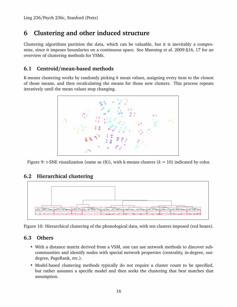
Clustering algorithms partition the data, which can be valuable, but it is inevitably a compro-mise, since it imposes boundaries on a continuous space. See Manning et al. 2009:§16, 17 for anoverview of clustering methods for VSMs.
6.1 Centroid/mean-based methods
K-means clustering works by randomly picking k mean values, assigning every item to the closestof those means, and then recalculating the means for those new clusters. This process repeatsiteratively until the mean values stop changing.
ɒɑ
ɶ
aæ
ʌ
ɔ
o ɤ
ɘ
œ
əә
e
ɞ
ø
ɛ
ɵ
ɯu
ʊ
ɨʉ
y i
ʏɪ
ŋ
ʟ
ɫ
ɴ
ʀ
ɲ
ʎ
ŋŋ
ʟʟ
ɳ
ʙ
ɭ
ɺ
ɻ
ɽr
nm
l
ɾ
ɱ
ʔɣx
kg
kxg ɣ
ħʕ
ʁq
χ
ɢ
ɕ
ɟ
ʝ
c
ç
dʑtç
ɣɣ
xx
k k
g g
ʑ
ʈ ɖ
ɬ
ʐ
ɸ
ʂ ʒ
z
v
t
ʃ
s
p
f
d
b
θ
ɮ
ð
β
dʒdz
dɮ
d ɮ tʃtɬ tstɬ ts
tɬ d zd ɮ ʈʂ
ɖʑ
pf bv
pɸbβ
tθdð
cçɟʝ
kxkxgɣ
g ɣqχɢʁ
ɧ
kpgb
pt
bd
ɰɰ
w ɥ
jɹ
ʋ
ʍ ɦh
Figure 9: t-SNE visualization (same as (8)), with k-means clusters (k = 10) indicated by color.
6.2 Hierarchical clustering
ɯ ɨj
ɰ ɰ i ɪ æ e ɛ ɑ a ʌ ɤ ɘ əә ɒ ɔ o w u ʊ ɥ ʉ y ʏ œ ɞ ɶ ø ɵ ɴ ŋ ɲ ŋ ŋ ɳ n m ɱ ʎ ʟ ʟ ʟɫ ɺ l ɽ ɾ ɹ ɭ ɻ ʋ ʀ ʙ r ɣ ɣ x x kx
kx gɣ
gɣ ɕ tç dʑ ʑɟ c cç ɟʝɧ ʝ ç x kx
qχ ħ χʕ ʁ ɣ gɣ
ɢʁ q ɢ k g kp gb k k g g ʈ ɖ t d pt bdʔ p b pɸ bβ pf
bv ɸf v β ʍ ɦ h dʒ tʃ ts
dz z s dz ts ʈʂ ɖʑ ʐ ʂ ʒʃ θ ð tθ dðɬ ɮ dɮ tɬ
dɮ tɬ tɬ dɮ
Figure 10: Hierarchical clustering of the phonological data, with ten clusters imposed (red boxes).
6.3 Others
• With a distance matrix derived from a VSM, one can use network methods to discover sub-communities and identify nodes with special network properties (centrality, in-degree, out-degree, PageRank, etc.).
• Model-based clustering methods typically do not require a cluster count to be specified,but rather assumes a specific model and then seeks the clustering that best matches thatassumption.
16
Ling 236/Psych 236c, Stanford (Potts)
7 (Semi-)supervision
The VSMs we’ve seen so far are not grounded. However, where information about the world isavailable, we can bring it in through a mix of unsupervised and supervised methods.
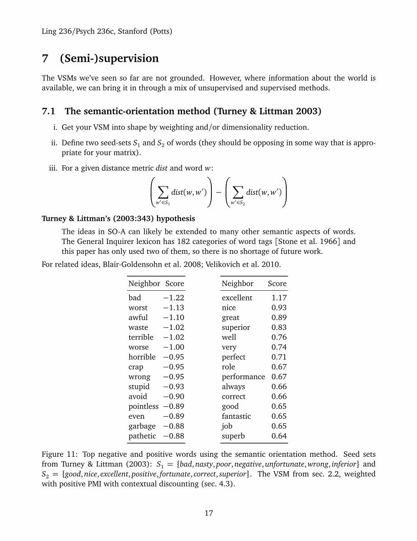
7.1 The semantic-orientation method (Turney & Littman 2003)
i. Get your VSM into shape by weighting and/or dimensionality reduction.
ii. Define two seed-sets S1 and S2 of words (they should be opposing in some way that is appro-priate for your matrix).
iii. For a given distance metric dist and word w:
∑
w′∈S1
dist(w, w′)
−
∑
w′∈S2
dist(w, w′)
Turney & Littman’s (2003:343) hypothesis
The ideas in SO-A can likely be extended to many other semantic aspects of words.The General Inquirer lexicon has 182 categories of word tags [Stone et al. 1966] andthis paper has only used two of them, so there is no shortage of future work.
For related ideas, Blair-Goldensohn et al. 2008; Velikovich et al. 2010.
Neighbor Score
bad −1.22worst −1.13awful −1.10waste −1.02terrible −1.02worse −1.00horrible −0.95crap −0.95wrong −0.95stupid −0.93avoid −0.90pointless −0.89even −0.89garbage −0.88pathetic −0.88
Neighbor Score
excellent 1.17nice 0.93great 0.89superior 0.83well 0.76very 0.74perfect 0.71role 0.67performance 0.67always 0.66correct 0.66good 0.65fantastic 0.65job 0.65superb 0.64
Figure 11: Top negative and positive words using the semantic orientation method. Seed setsfrom Turney & Littman (2003): S1 = {bad, nasty, poor, negative, unfortunate, wrong, inferior} andS2 = {good, nice, excellent, positive, fortunate, correct, superior}. The VSM from sec. 2.2, weightedwith positive PMI with contextual discounting (sec. 4.3).
17
Ling 236/Psych 236c, Stanford (Potts)
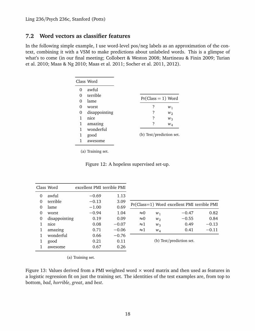
7.2 Word vectors as classifier features
In the following simple example, I use word-level pos/neg labels as an approximation of the con-text, combining it with a VSM to make predictions about unlabeled words. This is a glimpse ofwhat’s to come (in our final meeting; Collobert & Weston 2008; Martineau & Finin 2009; Turianet al. 2010; Maas & Ng 2010; Maas et al. 2011; Socher et al. 2011, 2012).
Class Word
0 awful0 terrible0 lame0 worst0 disappointing1 nice1 amazing1 wonderful1 good1 awesome
(a) Training set.
Pr(Class= 1) Word
? w1? w2? w3? w4
(b) Test/prediction set.
Figure 12: A hopeless supervised set-up.
Class Word excellent PMI terrible PMI
0 awful −0.69 1.130 terrible −0.13 3.090 lame −1.00 0.690 worst −0.94 1.040 disappointing 0.19 0.091 nice 0.08 −0.071 amazing 0.71 −0.061 wonderful 0.66 −0.761 good 0.21 0.111 awesome 0.67 0.26
(a) Training set.
Pr(Class=1) Word excellent PMI terrible PMI
≈0 w1 −0.47 0.82≈0 w2 −0.55 0.84≈1 w3 0.49 −0.13≈1 w4 0.41 −0.11
(b) Test/prediction set.
Figure 13: Values derived from a PMI weighted word × word matrix and then used as features ina logistic regression fit on just the training set. The identities of the test examples are, from top tobottom, bad, horrible, great, and best.
18

Ling 236/Psych 236c, Stanford (Potts)
8 Tools
• R has everything you need for matrices that will fit into memory.
• See Turney & Pantel 2010:§5 for lots of open-source projects.
• Python NLTK’s text and cluster: http://www.nltk.org/
• Python’s gensim is excellent for massive VSMs: http://radimrehurek.com/gensim/
• MALLET and FACTORIE: http://people.cs.umass.edu/~mccallum/code.html
ReferencesBaayen, R. Harald. 2001. Word frequency distributions. Dordrecht: Kluwer Academic Publishers.Baker, Kirk. 2005. Singular value decomposition tutorial. Ms., The Ohio State University. http://www.ling.
ohio-state.edu/~kbaker/pubs/Singular_Value_Decomposition_Tutorial.pdf.Blair-Goldensohn, Sasha, Kerry Hannan, Ryan McDonald, Tyler Neylon, George A. Reis & Jeff Reynar. 2008. Building
a sentiment summarizer for local service reviews. In Www workshop on nlp in the information explosion era (nlpix),Beijing, China.
Blei, David M. 2012. Probabilistic topic models. Communications of the ACM 55(4). 77–84.Blei, David M., Andrew Y. Ng & Michael I. Jordan. 2003. Latent dirichlet allocation. Journal of Machine Learning
Research 3. 993–1022.Church, Kenneth Ward & William Gale. 1995. Inverse dcument frequency (IDF): A measure of deviations from Poisson.
In David Yarowsky & Kenneth Church (eds.), Proceedings of the third acl workshop on very large corpora, 121–130.The Association for Computational Linguistics.
Collobert, Ronan & Jason Weston. 2008. A unified architecture for natural language processing: Deep neural networkswith multitask learning. In Proceedings of the 25th international conference on machine learning ICML ’08, 160–167. New York: ACM. doi:http://doi.acm.org/10.1145/1390156.1390177. http://doi.acm.org/10.1145/1390156.1390177.
Van de Cruys, Tim. 2009. A non-negative tensor factorization model for selectional preference induction. In Proceedingsof the workshop on geometrical models of natural language semantics, 83–90. Athens, Greece: ACL.
Deerwester, S., S. T. Dumais, G. W. Furnas, T. K. Landauer & R. Harshman. 1990. Indexing by latent semantic analysis.Journal of the American Society for Information Science 41(6). 391–407. doi:10.1002/(SICI)1097-4571(199009)41:6<391::AID-ASI1>3.0.CO;2-9.
Dice, Lee R. 1945. Measures of the amount of ecologic association between species. Ecology 26(3). 267–302.Firth, John R. 1935. The technique of semantics. Transactions of the Philological Society 34(1). 36–73.Firth, John R. 1957. A synopsis of linguistic theory 1930–1955. In Studies in linguistic analysis, 1–32. Oxford:
Blackwell.Furnas, G. W., Thomas K. Landauer, L. M Gomez & S. T. Dumais. 1983. Statistical semantics: Analysis of the potential
performance of keyword information systems. Bell System Technical Journal 62(6). 1753–1806.Harris, Zellig. 1954. Distributional structure. Word 10(23). 146–162.Kennedy, Christopher. 2007. Vagueness and grammar: The semantics of relative and absolute gradable adjective.
Linguistics and Philosophy 30(1). 1–45.Kennedy, Christopher & Louise McNally. 2005. Scale structure and the semantic typology of gradable predicates.
Language 81(2). 345–381.Lee, Lillian. 1999. Measures of distributional similarity. In Proceedings of the 37th annual meeting of the association for
computational linguistics, 25–32. College Park, Maryland, USA: ACL. doi:10.3115/1034678.1034693.Lin, Dekang & Patrick Pantel. 2001. DIRT – discovery of inference rules from text. In Proceedings of ACM SIGKDD
conference on knowledge discovery and data mining, 323–328. New York: ACM.Maas, Andrew, Andrew Ng & Christopher Potts. 2011. Multi-dimensional sentiment analysis with learned representa-
tions. Ms., Stanford University.Maas, Andrew L. & Andrew Y. Ng. 2010. A probabilistic model for semantic word vectors. In Nips 2010 workshop on
deep learning and unsupervised feature learning, .
19

Ling 236/Psych 236c, Stanford (Potts)
van der Maaten, Laurens & Hinton Geoffrey. 2008. Visualizing data using t-SNE. Journal of Machine Learning Research9. 2579–2605.
Manning, Christopher D., Prabhakar Raghavan & Hinrich Schütze. 2009. An introduction to information retrieval.Cambridge University Press.
Manning, Christopher D. & Hinrich Schütze. 1999. Foundations of statistical natural language processing. Cambridge,MA: MIT Press.
Martineau, Justin & Tim Finin. 2009. Delta TFIDF: An improved feature space for sentiment analysis. In Thirdinternational AAAI conference on weblogs and social media, 258–261. AAAI Press.
Pantel, Patrick & Dekang Lin. 2002. Discovering word senses from text. In Proceedings of the eighth ACM SIGKDDinternational conference on knowledge discovery and data mining KDD ’02, 613–619. New York: ACM. doi:http://doi.acm.org/10.1145/775047.775138.
Ramage, Daniel, Susan Dumais & Dan Liebling. 2010. Characterizing microblogs with topic models. In Proceedingsof the international AAAI conference on weblogs and social media, 130–137. Washington, D.C.: Association for theAdvancement of Artificial Intelligence.
Ramage, Daniel, David Hall, Ramesh Nallapati & Christopher D. Manning. 2009. Labeled LDA: A supervised topicmodel for credit attribution in multi-labeled corpora. In Proceedings of the 2009 conference on empirical methods innatural language processing, 248–256. Singapore: ACL.
van Rijsbergen, Cornelis Joost. 1979. Information retrieval. London: Buttersworth.Salton, Gerald, Andrew Wong & Chung-Shu Yang. 1975. A vector space model for automatic indexing. Communications
of ACM 18(11). 613–620.Socher, Richard, Brody Huval, Christopher D. Manning & Andrew Y. Ng. 2012. Semantic compositionality through
recursive matrix-vector spaces. In Proceedings of the 2012 conference on empirical methods in natural languageprocessing, 1201–1211. Stroudsburg, PA.
Socher, Richard, Jeffrey Pennington, Eric H. Huang, Andrew Y. Ng & Christopher D. Manning. 2011. Semi-supervisedrecursive autoencoders for predicting sentiment distributions. In Proceedings of the 2011 conference on empiricalmethods in natural language processing, 151–161. Edinburgh, Scotland, UK.: ACL.
Steyvers, Mark & Tom Griffiths. 2006. Probabilistic topic models. In Thomas K. Landauer, D McNamara, S Dennis &W Kintsch (eds.), Latent semantic analysis: A road to meaning, Lawrence Erlbaum Associates.
Stone, Philip J, Dexter C Dunphry, Marshall S Smith & Daniel M Ogilvie. 1966. The General Inquirer: A computerapproach to content analysis. Cambridge, MA: MIT Press.
Stubbs, Michael. 1993. British traditions in text analysis — from Firth to Sinclair. In Mona Baker, Gill Francis & ElenaTognini-Bonelli (eds.), Text and technology: In honour of John Sinclair, 1–33. John Benjamins.
Syrett, Kristen, Christopher Kennedy & Jeffrey Lidz. 2009. Meaning and context in children’s understanding of grad-able adjectives. Journal of Semantics 27(1). 1–35.
Syrett, Kristen & Jeffrey Lidz. 2010. 30-month-olds use the distribution and meaning of adverbs to interpret noveladjectives. Language Learning and Development 6(4). 258–282.
Turian, Joseph, Lev-Arie Ratinov & Yoshua Bengio. 2010. Word representations: A simple and general method forsemi-supervised learning. In Proceedings of the 48th annual meeting of the association for computational linguistics,384–394. Uppsala, Sweden: ACL.
Turney, Peter D. 2007. Empirical evaluation of four tensor decomposition algorithms. Tech. Rep. ERB-1152 Institutefor Information Technology, National Research Council of Canada.
Turney, Peter D. & Michael L. Littman. 2003. Measuring praise and criticism: Inference of semantic orientationfrom association. ACM Transactions on Information Systems (TOIS) 21. 315–346. doi:http://doi.acm.org/10.1145/944012.944013.
Turney, Peter D., Michael L. Littman, Jeffrey Bigham & Victor Shnayder. 2003. Combining independent modulesto solve multiple-choice synonym and analogy problems. In Proceedings of the international conference on recentadvances in natural language processing, 482–489. Borovets, Bulgaria.
Turney, Peter D. & Patrick Pantel. 2010. From frequency to meaning: Vector space models of semantics. Journal ofArtificial Intelligence Research 37. 141–188.
Velikovich, Leonid, Sasha Blair-Goldensohn, Kerry Hannan & Ryan McDonald. 2010. The viability of web-derivedpolarity lexicons. In Human language technologies: The 2010 annual conference of the north american chapter of theassociation for computational linguistics, 777–785. Los Angeles: ACL.
Weaver, Warren. 1955. Translation. In William N. Locke & A. Donald Booth (eds.), Machine translation of languages:Fourteen essays, 15–23. Cambridge, MA: MIT Press.
20