Diversification, Cost Structure, and the Risk

Premium of Multinational Corporations∗

Jose L. Fillat†

Federal Reserve Bank of Boston

Stefania Garetto‡

Boston University

Lindsay Oldenski§

Georgetown University

February 19, 2015

Abstract

We investigate theoretically and empirically the relationship between the ge-ographic structure of a multinational corporation and its risk premium. Ourstructural model suggests two channels. On the one hand, multinational ac-tivity offers diversification benefits: risk premia should be higher for firmsoperating in countries where shocks co-vary more with the domestic ones.Second, hysteresis and operating leverage induced by fixed and sunk costsof production imply that risk premia should be higher for firms operating incountries where it is costlier to enter and produce. Our empirical analysis con-firms these predictions and delivers a decomposition of firm-level risk premiainto individual countries’ contributions.Keywords: Multinational firms, diversification, risk premium, stock returns.JEL Classification: F14, F23, G12.

∗The statistical analysis of firm-level data on US multinational companies was conducted at theBureau of Economic Analysis, US Department of Commerce under arrangements that maintainlegal confidentiality requirements. The views expressed are those of the authors and do not reflectofficial positions of the US Department of Commerce, of the Federal Reserve Bank of Bostonor the Federal Reserve System. The authors would like to thank William Zeile and RaymondMataloni for assistance with the BEA data. We are also grateful to Maggie Chen, Fritz Foley,Simon Gilchrist, Raoul Minetti, Eduardo Morales, Marc Muendler, Alan Spearot, the editor, twoanonymous referees, and seminar participants at ASU, BC, Brown, BU, Columbia, Georgetown,the Federal Reserve Banks of Boston, Dallas and Richmond, EITI 2013 (Bangkok), LMU Munich,the Midwest International Trade Meetings 2013, MIT, the NBER ITI 2014 Spring Meetings, PSE,SED 2013 (Seoul), SCIEA 2013, and WAITS 2013 for their helpful comments.

†Federal Reserve Bank of Boston, 600 Atlantic Avenue, Boston MA 02210. E-mail:Jose.Fillat@bos.frb.org.

‡Department of Economics, Boston University, 270 Bay State Road, Boston, MA 02215. E-mail:garettos@bu.edu.

§Georgetown University, Intercultural Center 515, 37th and O Streets, NW Washington DC,20057. E-mail: lo36@georgetown.edu.

1

1 Introduction

A large literature on foreign direct investment has studied how firms decide whether

to become multinational corporations (henceforth, MNCs) and which countries to

enter. Still, little is known about the consequences of these decisions for firm-level

risk. Do firms’ activities in foreign countries reduce the risk that investors bear

through diversification? Or are there characteristics of MNCs that increase their

risk relative to purely domestic firms? How does firm risk-exposure depend on the

countries in which a firm operates? To address these questions, we analyze how the

geographic structure of a multinational corporation impacts its risk premium in the

stock market.1 The answer is complex, as firms’ foreign activities can be both a

source of diversification and a source of risk to their investors.

MNCs are the largest players in the world economy. Understanding their risk

exposure sheds light on the global allocation of risk across countries. This is es-

pecially important in consideration of recent economic events like the crisis, whose

global aspect puts at the forefront of economic analysis the map of economic linkages

across countries.

Theoretically, a firm’s decisions about which countries to enter affects the risk

premium via two channels. On the one hand, operating an affiliate in a foreign

country induces diversification and reduces risk exposure. On the other hand, sunk

entry costs and fixed operating costs generate hysteresis and leverage that increase

risk exposure. Under the assumptions that agents are rational and markets are

efficient, in equilibrium, risk averse agents require a risk premium that is higher the

higher the risk exposure of the firms they invest into.

Empirically, we focus on differences in risk premia across firms that differ in the

set of countries in which they operate. To do so, we exploit a rich firm-level dataset

on MNCs with detailed information about firms’ foreign operations by country,

accounting, and financial market data. Consistent with the predictions of the model,

we find that firms operating in countries whose GDP shocks co-move more with

those of the US and in countries with higher fixed and sunk entry costs exhibit

systematically higher risk premia.

The theoretical underpinning of our analysis is a streamlined, multi-country ver-

sion of the model developed by Fillat and Garetto (2014), which links firms’ interna-

1Stock returns in excess of the risk-free rate define the risk premium of a firm.

2

tional activities with their stock market returns.2 This approach to the multinational

firm problem is, essentially, an asset pricing problem in which the generating pro-

cess for consumption and cash flows are needed to price the firm. In the model,

multinational activity offers diversification potential: if the business cycles of two

countries are not perfectly correlated, multinational sales diversify away the risk

arising from country-specific fluctuations and reduce firms’ returns in equilibrium.

This mechanism, referred to as the “diversification channel”, implies that, in equi-

librium, MNCs should exhibit lower expected returns than non-multinational firms

– all else equal. Within multinationals, returns should be higher for those firms

operating in countries whose business cycles co-vary more with the one of the US.

Moreover, the model introduces another channel of risk, arising from hysteresis and

potential losses induced by sunk entry costs and fixed operating costs, which make

firms leveraged. Firms open affiliates abroad when prospects of growth make foreign

operations profitable, but they must bear sunk entry costs to open an affiliate, and

fixed costs of production. If the host country is hit by a negative shock, the affiliate

may incur losses. The parent may find optimal not to exit the foreign market and

bear those losses for a while, in order not to forego the sunk cost it paid to enter.

The higher the fixed and sunk costs of production, the higher the potential losses

and the longer the time for which a firm is willing to bear them. These potential

losses are perceived as a cash flow risk by the investors. This second mechanism,

which we refer to as the “fixed and sunk cost channel”, implies that MNCs with

affiliates in countries where entry is more costly and fixed operating costs are higher

should exhibit higher stock returns than MNCs with affiliates located in countries

that are more easily and cheaply accessible. To our knowledge, our paper is the first

one to study the relationship between the endogenous location choices of a MNC and

its risk exposure. Given that MNCs are the largest players in the global economy,

understanding this relationship is key to evaluating the allocation of aggregate risk

across countries.

Our empirical analysis exploits a novel dataset obtained by merging accounting

and financial data from Compustat/CRSP with the US Bureau of Economic Analysis

(BEA) data on the operations of multinational corporations. The data display a

2Our model builds on the literature on investment under uncertainty, particularly on the realoption value framework developed by Dixit (1989) and Dixit and Pindyck (1994) as applied to aneconomy with heterogeneous firms by Fillat and Garetto (2014).

3

large amount of variation across MNCs in terms of number, characteristics, and

location of foreign affiliates, allowing us to study the cross-section of returns of

MNCs and to relate it to firm- and country-level characteristics.

We start with a reduced form specification whose goal is to explore the statisti-

cal relationship between measures of diversification, entry costs, and returns. The

results of our regression analysis are consistent with the predictions of the model:

GDP growth covariances and entry costs in the countries in which firms have affili-

ates are positively correlated with the returns that firms offer in the stock market.

These results are robust to controlling for the impact that potential activities in

countries other than the ones currently served have on the returns of the firm (the

option value).

The model at the heart of our analysis delivers a structural equation linking ex-

pected returns to firm- and country-level characteristics. By estimating this equation

we are able to quantify the effect of the geographic choices of a MNC on its risk

premium. This specification allows us to decompose firm-level risk premia along two

dimensions. First, we compute the contribution of each host country to the firms’

risk premium. Second, we separate the contribution of option value versus assets in

place in explaining stock returns.

By aggregating our estimates, we show that the aggregate risk premium from

multinational sales is large: a firm with affiliates in every country in our sample

has, on average, expected annual returns that are about 3% higher than those of

a purely domestic firm. The countries that are associated with the highest risk

premia are Greece, Malaysia, Singapore, Denmark, India and China, while most

European countries and Canada are associated with relatively low risk premia. The

aggregate risk premium coming from the option value of foreign sales is smaller but

also significant, at 0.65 %, indicating that the mere possibility of entering foreign

markets is a source of risk to the firm.

The question of understanding why and how average stock returns vary across

firms based on certain characteristics is central to the asset pricing literature.3

Nonetheless, very little empirical work has been done on the returns of multinational

3An extensive literature in finance has been investigating cross-sectional differences in stockreturns across firms, assets, or portfolios, identifying several variables driving returns differen-tials. Fama and French (1996) provide comprehensive evidence about returns differentials acrossportfolios formed according to particular characteristics like size and book-to-market.

4

corporations. Early research examined the returns of MNCs to assess whether firms’

foreign activities provide diversification benefits to their stockholders. Support for

this “diversification hypothesis” is scarce: Jacquillat and Solnik (1978) regressed the

returns of multinationals from nine countries on a set of market indices and found

that multinational returns tended to covary most with the firm’s home market,

hence not providing any evidence in support of diversification. Senchack and Bee-

dles (1980) compared the risk, returns and betas of portfolios of multinationals with

portfolios of domestic and international equities and found that multinationals did

not deliver diversification benefits. Using a different methodology based on mean-

variance spanning tests, Rowland and Tesar (2004) also found limited evidence of

diversification benefits for MNCs. More recently, using a sample of manufacturing

firms from Compustat, Fillat and Garetto (2014) have shown that the stock mar-

ket returns of multinational corporations are systematically higher than the stock

market returns of non-multinational firms, also against what would be predicted by

the diversification hypothesis. The structural model in Fillat and Garetto (2014)

sheds light on this “puzzle” by introducing another channel, the fixed and sunk

cost channel, that increases the risk to which MNCs are exposed compared to non-

multinational firms and can potentially explain MNCs’ higher returns and the lack

of evidence of diversification.

Our analysis is related to an extensive literature on foreign direct investment,

which has documented important differences across firms in their choice of geo-

graphic locations, and to empirical research using the BEA data on the operations

of multinational corporations, starting with Kravis and Lipsey (1982) and Brainard

(1997), and more recently Yeaple (2003), Helpman, Melitz, and Yeaple (2004), and

Yeaple (2009).4 In a model with similar ingredients but different assumptions, Ra-

mondo, Rappoport, and Ruhl (2013) study selection into export and FDI in the

presence of aggregate uncertainty. We see our analysis as complementary to theirs,

as we emphasize the relationship between firms’ global decisions and financial vari-

ables rather than the role of uncertainty for selection.

To our knowledge, this is the first paper to link the geographic information con-

tained in the BEA data to stock market data from CRSP.5 By their nature, stock

4See also Chen and Moore (2010) and Alfaro and Chen (2013).5Branstetter, Fisman, and Foley (2006) merge the BEA data on the operations of US multina-

tionals with accounting data from Compustat to examine the effect of IPR reforms on technology

5

market data are forward-looking, and incorporate information about agents’ expec-

tations that can be informative about the long-run outcomes of these firms. While

bringing novel data into the analysis, we contribute to the literature by providing

new insights on the operations of MNCs from a financial markets, forward-looking

perspective.

Our work is also related to a strand of literature in corporate finance that studies

the linkages between international activity and stock market variables.6 Our analysis

departs from these contributions by taking into account the full geographic structure

of the firm as a determinant of stock returns, and by starting from the predictions

of a structural model to identify the economic forces that link MNCs’ structure and

stock returns in the data.

The rest of the paper is organized as follows. Section 2 lays out the theoretical

model at the basis of our empirical specification. Section 3 describes the finan-

cial data and the data on the operations of multinational corporations. Section 4

presents our baseline empirical specifications and results, and Section 5 concludes.

The derivation of the model and several robustness exercises are relegated to the

appendix.

2 The Returns of Multinational Corporations

The model we develop in this section is designed to illustrate how the stock returns of

multinational corporations depend on a set of variables related to their international

activities across countries. At the aggregate level, the model is specified as an

endowment economy, consistent with consumption-based asset pricing models. We

take aggregate consumption as given, and focus on modeling the production side

of the economy, where firms’ valuations are affected by firm-level and country-level

characteristics. Firms’ valuations and the covariance of their profits with the agents’

marginal utility drive the returns.

The model is a multi-country extension of the framework developed in Fillat and

Garetto (2014).7 The economy is composed byN+1 countries: a Home country, that

transfer within multinational corporations.6See Denis, Denis, and Yost (2002) and Baker, Foley, and Wurgler (2009).7While Fillat and Garetto (2014) distinguish entry in foreign markets according to whether it

happens via export or FDI, due to data availability in this paper we disregard the decision to

6

we denote by h, and N potentially asymmetric foreign countries, that we denote by

j = 1, ...N . Time is continuous. Each country is hit by aggregate shocks to its GDP

growth rate, which are described by the following geometric Brownian motions:8

dYiYi

= µidt+ σidzi, for i = h, j and j = 1, ...N (1)

where µi ≥ 0, σi > 0. Yi denotes the GDP level in country i and dzi is the

increment of a standard Wiener process. GDP growth processes may be correlated

across countries: let ρj ∈ [−1, 1] denote the correlation between the GDP growth of

the Home country and the one of country j.

International markets are incomplete: changes in aggregate consumption in each

country are equal to changes in GDP, and there is no possibility of consumption

smoothing over time or across countries. We assume complete home bias in the asset

markets, in the sense that firms are owned by agents in country h, who discount

cash flows with the following discount factor Mh:9

dMh

Mh

= −rhdt− γσhdzh (2)

where rh denotes the risk-free rate in the Home country and γ denotes risk-aversion.10

This is a partial equilibrium model where aggregate quantities are taken as given.

export and focus on the choice of becoming a multinational corporation.8It is well accepted that equilibrium consumption growth follows a random walk since Hall

(1978). The unit root process is necessary to generate an option value component in the valueof the firm. We take standard deviations and correlations of consumption growth as exogenousparameters, and model firm’s decisions depending on those parameters. In general equilibrium,firms’ international activities could have an impact on host country-level variables, hence the GDPgrowth correlations ρj would be endogenous. In our data, total MNCs’ sales to a host countryare typically a very small fraction of the host country’s GDP (3.3% on average), hence we arguethat it is acceptable to take the GDP growth correlations as exogenous. For a different approachwhere country-specific volatility is endogenous and affected by international activity, see Caselliet al. (2014).

9The model does not allow for any possibility of international portfolio diversification, butfeatures perfect home bias in equity portfolios. This assumption is not at odds with the data:Tesar and Werner (1998) provide evidence of an extreme home bias in equity portfolios: about90% of US equity was invested in the US stock market in the mid-1990s. Atkeson and Bayoumi(1993), Sorensen and Yosha (1998), and Crucini (1999) present evidence supporting the assumptionof international market incompleteness.

10The process for the stochastic discount factor or intertemporal marginal rate of substitution,Mh, is an equilibrium object that can be derived from agents maximizing CRRA utility overaggregate consumption.

7

Therefore, equilibrium in the goods and asset markets is determined by adjustment

in prices.

Aggregate output in each country Yi is produced by domestic firms and by the

affiliates of multinational firms located in country i. Each firm chooses its optimal

production level in each country as a share of total output Yi.

Let V denote the value of a firm. V depends on firm-specific characteristics, like

productivity, size, employment, etc., and on country-specific characteristics, like the

GDP growth processes of the countries where the firm operates, entry costs, and

other operating costs. For this reason, we write V = V(a, Y , X), where a denotes

firm-specific characteristics, Y = (Yh, Y1, ...YN) denotes a vector whose entries are

the realizations of GDP described by Eq. (1), and X = (Xh, X1, ...XN) denotes a

vector whose entries are other country-specific characteristics affecting firm value.

Consistent with the literature on selection into multinational activity and with the

empirical evidence on firms’ international dynamics, fixed operating costs of pro-

duction and sunk costs of entry into a market are particularly relevant among the

variables entering the vector X.11 Depending on its characteristics a, each firm

self-selects into the set of countries where its operations are profitable. Given de-

mand for each firm’s product in each country, a drives both the intensive margin of

production in each country and the extensive margin of entry in different countries.

We assume that firms’ activities are independent across countries, i.e. each

firm makes entry and production decisions country-by-country.12 Since the decision

of setting up a foreign affiliate is endogenous and affected by uncertainty through

the country-specific GDP growth shocks, we must consider the fact that a firm’s

valuation is affected both by its assets currently in place in various countries, and

by the possibility of entering new countries (its option value).13 For these reasons

11Helpman, Melitz, and Yeaple (2004) model selection into multinational activity as motivated bythe interaction of high productivity and fixed costs. The importance of fixed costs for multinationalproduction is documented in the empirical work of Brainard (1997). Roberts and Tybout (1997)and Das, Roberts, and Tybout (2007) show the empirical relevance of sunk costs for entry inforeign markets.

12The model does not accommodate the possibility of export platforms, whereby foreign affiliatesof a multinational corporation export to third countries. As a result, a multinational firm isessentially a “portfolio” of assets in different countries, linked only by the fact that each segmentof the firm operates with the same firm-level characteristics a.

13To understand why the option value enters the value of a firm, it is useful to recall that thevalue of a firm is the present discounted value of its profits over an infinite time horizon. If a firmis not selling in a market today but maybe it will be in the future, this possibility has a value and

8

we write the value of the firm as:

V(a, Y , X) = Vh(a, Yh, Xh) +∑

j∈A

Vj(a, Yj, Xj) +∑

j 6∈A

V oj (a, Yj, Xj) (3)

where Vh(a, Yh, Xh) denotes the firm’s value of domestic sales, Vj(a, Yj, Xj) denotes

the value of the firm’s affiliate sales in country j if the firm has an affiliate there,

and V oj (a, Yj, Xj) denotes the option value of the firm’s affiliate sales in country j if

the firm does not have an affiliate there. A denotes the endogenous set of countries

where the firm has affiliates (A ⊆ {1, 2, ...N}).

We assume that all firms sell in the Home country. Conversely, firms’ entry and

exit into foreign markets are endogenous. For these reasons, over a generic time

interval ∆t we can express the components of a firm’s value function as:

Vh(a, Yh, Xh) = πh(a, Yh, Xh)M∆t + E[M∆t · Vh(a, Y′h, Xh|Yh)] (4)

Vj(a, Yj, Xj) = max{πj(a, Yj, Xj)M∆t + E[M∆t · Vj(a, Y

′j , Xj|Yj)] ; ...

... V oj (a, Yj, Xj)

}(5)

V oj (a, Yj, Xj) = max

{E[M∆t · V o

j (a, Y′j , Xj|Yj)] ; Vj(a, Yj, Xj)− Fj

}(6)

where πi(a, Yi, Xi) denotes the flow profits of the firm in country i (for i = h, j and

j = 1, ...N), Fj denotes the sunk entry cost that a firm has to cover to open an

affiliate in country j, and the terms in expectations indicate the firm’s continuation

value in the event in which its status in a country does not change (i.e. it does not

enter or exit the country).

We show in Appendix A that, in the continuation regions, the three components

of the value functions above satisfy the following no-arbitrage conditions:

πh − rhVh + (µh − γσ2h)YhVh

′Y dt+

1

2σ2hY

2h Vh

′′Y = 0 (7)

πj − rhVj + (µj − γρjσhσj)YjVj′Ydt+

1

2σ2jY

2j Vj

′′Y

= 0 (8)

−rhVoj + (µj − γρjσhσj)YjV

oj′

Ydt+

1

2σ2jY

2j V

oj′′

Y= 0 (9)

where the dependence of profits and values on (a, Y , X) has been suppressed to ease

must be reflected in the value function. Dixit (1989) provides a seminal treatment of the optionvalue of entry in a model of investment under uncertainty and sunk costs.

9

the notation. Given functional forms for each firm’s demand in each market, one

can solve explicitly for the value functions using a system of value-matching and

smooth-pasting conditions. This system also delivers the country- and firm-specific

thresholds in the realizations of the shocks that induce entry into a country or exit

from it. The explicit solution of this problem is beside the scope of this paper,

but we illustrate it in Appendix A, as it helps to link the model to the empirical

analysis.14

By combining Eqs. (7)-(9) one can obtain the following expression for a multi-

national’s expected returns:15

E(ret) ≡

πh +∑

j∈A

πj + E(dV)

V= rh + γ

(

σ2hYhVh

′Y

V+∑

j∈A

σhσjρjYjVj

′Y

V+ ...

...∑

j 6∈A

σhσjρjYjV

oj′

Y

V

)

. (10)

Eq. (10) summarizes the implications of the model for the dependence of firm

level returns (and hence of the risk premium E(ret)− rh) on country-specific vari-

ables, and is the theoretical foundation of our empirical specifications. The risk

aversion, γ, captures the price of risk for the representative agent, or how much

does he need to be rewarded for additional exposure to risk incurred by the firms.

The terms in the parentheses capture the three sources of risk that a firm is exposed

to: domestic risk, risk from the countries where the firm has an affiliate, and risk

from the countries where the firm has the option of opening an affiliate, respectively.

The first term of the expression describes the contribution of domestic activities to

the returns. The last term captures the option value of entry in new countries,

which we will approximate in our empirical analysis. We now focus on the second

term, which we refer to as “assets in place”. This term captures the exposure of

multinational firms to the risk that arises from having affiliates in foreign countries,

and generates two testable implications.

First, Eq. (10) indicates that expected returns should be higher the higher the

covariances σhσjρj between the Home country’s GDP growth rate and the GDP

14See Fillat and Garetto (2014) for more details.15Details of the calculations are relegated to Appendix A.

10

growth rates of the host countries. This prediction summarizes the effect of diversi-

fication on returns in the model: the more the GDP growth rates of two countries

co-vary, the smaller the amount of diversification that foreign activities provide. As

a result, MNCs with affiliates in countries whose GDP growth rates co-move more

with the US GDP growth rate are less diversified (and more risky) than MNCs with

affiliates in countries whose GDP growth rates co-move less with that of the US.

Riskier firms command higher expected returns in equilibrium.

Second, the fact that a firm has activities in a foreign country indicates that the

firm paid an entry cost to establish an affiliate there and is bearing fixed operating

costs.16 These costs, which are independent of firm size, affect a firm’s value but not

its derivative V ′. In other words, the elasticity of the value function in host country

j (the term YjVj′Y/V) is increasing in the fixed and sunk costs of production, and Eq.

(10) indicates that expected returns should be higher the higher the fixed and sunk

costs of production in the host countries where the firm operates. The economic

intuition behind this prediction is the following: due to sunk entry costs and fixed

costs of production, if a host country is hit by a negative shock, the foreign affiliate

of a multinational firm may incur losses. The parent may find optimal not to exit

the foreign market and bear those losses for a while, in order not to forego the

sunk cost it paid to enter. The extent and duration of these losses are positively

correlated with the size of fixed and sunk costs. Investors perceive as a risk the

possibility of losses, and this cash flow risk must be rewarded by higher expected

returns in equilibrium. The analysis in Section 4 tests the empirical validity of these

predictions.17

It is important to notice that, even if Eq. (10) is derived from a simple power-

utility i.i.d. framework, the qualitative predictions of the model are robust to alter-

native, more sophisticated specifications, namely the inclusion of permanent shocks

16Due to data availability, we consider a firm to be operating in country j only if it has an affiliatethere. If a firm only exports to a country, we have no information about its activities there, hencewe cannot include the country in the set A. This leads us to underestimate the contribution ofassets in place to the risk premium of the firm, and to interpret our results as a lower bound ofthe amount of riskiness that operating in foreign markets generates.

17Our empirical analysis focuses on the relationship between the extensive margin of entry bycountry and the returns. If one had to parameterize the model using CES demand functions andlinear cost functions (like in most of the new trade literature), the model would also imply that –keeping the extensive margin of countries constant – returns should be increasing in the unit costof the firm. For the purpose of this paper we don’t test this prediction but we limit our analysisto test the extensive margin predictions of the model.

11

to GDP growth rates (“long-run risk”), disaster risk, recursive preferences, and the

addition of firm-specific productivity shocks. These alternative specifications affect

the solution of the value functions, but not the general dependence of returns on

covariances and fixed and sunk costs.

3 Data

To test the predictions of the model, we need information on multinational compa-

nies’ operations across countries and on their stock returns. We also need country-

level data on the covariance of GDP growth rates and on fixed and sunk costs of

production.

The Bureau of Economic Analysis collects firm-level data on US multinational

companies’ operations in its annual surveys of US direct investment abroad. All US

headquartered firms that have at least one foreign affiliate and meet a minimum size

threshold are required by law to respond to these surveys. The data include detailed

information on the firms’ operations both in the US and at their foreign affiliates.

Our empirical analysis uses information from the BEA data on the countries in which

each firm has operations. We also use data on the sales by each foreign affiliate,

as well as total global sales by the MNCs to control for the scale of operations in

each location and by each firm. The BEA surveys cover both manufacturing and

nonmanufacturing industries, classified according to BEA versions of 3-digit SIC

codes. We include firms in all industries and use data from 1987 through 2009.

Stock market returns data are obtained from the Center for Research in Security

Prices (CRSP), which includes information on all firms that are publicly traded in

the US stock market.18 We match the firm level stock return data from CRSP with

the firm level data on multinational operations from the BEA to obtain a set of

publicly traded US-headquartered multinational firms. To ensure that outlier firms

are not biasing our results, we drop observations that fall into the highest or lowest

5% in terms of their annual stock market returns. The result is a sample of more

than 3200 multinational firms operating in 118 countries and 148 industries over the

23 year period.

18The CRSP population includes NYSE, AMEX, and NASDAQ. We identify firm-level returnswith the returns of the firm’s common equity. Stock market expected returns in excess of the riskfree rate are the empirical counterpart of the risk premium.

12

The model emphasizes two channels that link firms’ foreign activities with their

stock market returns. To measure the diversification channel, we construct a firm-

level measure, Covft, of the extent to which GDP growth in each host country of

firm f co-varies with GDP growth in the home country (the US). We begin with

data on real GDP growth rates by country from the IMF. We assume that expected

GDP growth is constant. We then compute the covariance between annual US GDP

growth and annual GDP growth in each country over our sample period, resulting

in a time-invariant GDP growth covariance measure for each country, Covj . We use

these covariances together with information on firm f ’s affiliate sales to construct

our firm-level measure as a weighted average of the GDP growth covariances for the

countries in which the firm has foreign affiliates, where the share of sales by the

affiliates in each country are used as weights:

Covft =∑

j∈Af

sfjtCovj (11)

where Covj is the country-level GDP growth covariance and sfjt is the share of total

sales by foreign affiliates of firm f that were produced in country j in year t.19

To measure the fixed and sunk cost channel, we use country level data on the

cost of starting a business from the World Bank’s Doing Business database. Doing

Business records the costs and procedures officially required, or commonly done in

practice, for an entrepreneur to start up and formally operate an industrial or com-

mercial business. The information used to construct these data comes from official

laws, regulations and publicly available information on business entry, and the data

are verified in consultation with local incorporation lawyers, notaries and govern-

ment officials. The database includes information on various aspects of the cost of

starting a business, including initial capital requirements, license and registration

fees, number of startup procedures that must be undertaken, and the amount of

time these procedures usually require. Our primary specification uses the paid in

19Weighting the covariances by sales shares is the simplest and most intuitive way to obtainfirm-level measures of covariances with host countries. In Eq. (10) the covariances enter in adifferent way, where the “weights” that the model generates are the country-specific elasticities ofthe value function. The model-based estimation we perform in Section 4.3 mimics more closelythe structure of Eq. (10). We use the measure defined in Eq. (11) in our baseline specifications,but for our robustness tests we also conduct the empirical analysis using GDP growth correlationsrather than covariances. The results are reported in Appendix B.

13

minimum capital requirement. Doing Business defines this as “the amount that the

entrepreneur needs to deposit in a bank or with a notary before registration and

up to 3 months following incorporation, recorded as a percentage of the economy’s

income per capita.” We convert this measure to a US dollar value by multiplying

by income per capita. We use this variable to construct a firm-level measure of sunk

costs. As with the GDP growth correlations, the firm-level sunk cost variable is a

weighted average of the doing business measures for the countries in which the firm

has foreign affiliates, where the share of sales by the affiliates in each country are

used as weights:

Fft =∑

j∈Af

sfjtFj (12)

where Fj is a measure of cost to start a business in country j. For robustness, we

also construct a firm-level measure of sunk costs that uses the share of affiliates the

firm has in each country, rather than the sales share, as weights.20 We also use

alternative measures of entry costs, including the number of procedures required to

start a business, and the number of days these procedures take to complete.

Table 1 provides summary statistics for the firms in our dataset. We will be

using data on the entire sample of firms, as well as data on only the subset of firms

that can be classified as purely horizontal multinationals. In our model FDI sales are

only of the horizontal type, so by restricting our sample to purely horizontal firms

we prevent the possibility that our results are biased by different motives for FDI,

which could have different implications for risk. We define purely horizontal firms

as those firms for which at least 99% of sales by foreign affiliates are to the local

market in which the affiliate resides. Using this definition, about 26% of the firms

in our sample can be classified as purely horizontal MNCs.21 Most MNCs exhibit

some combination of horizontal, vertical, and export platform FDI. In our merged

dataset, about 94% of the firms have at least some horizontal sales, 66% have some

sales back to the US, and 65% have some sales to third countries. In terms of total

volumes of sales, about 64% of all sales by foreign affiliates are horizontal, about

20If a MNC needs to pay a sunk cost every time it opens a new affiliate (even in countries whereit already operates other affiliates), weighting by the number of affiliates may be the appropriatechoice. Results of the robustness checks using alternative definitions of Covft and Fft are reportedin Appendix B.

21In Appendix B we report the results of a robustness test using an alternative, looser definitionof horizontal MNCs.

14

Table 1: Summary Statistics.

N. Obs Mean Std. Dev. Min Max

ALL FIRMS

Tot. firm sales ($b) 21809 4.952 18.3 (confidential)Tot. affiliate sales by firm ($b) 21809 1.82 10.3 (confidential)No. of affiliates 21809 19.385 52.661 (confidential)No. of host countries 21809 9.428 12.437 (confidential)Annual Returns (%) 21809 11.296 42.015 -98.986 1315.79Covariance (Covft) 21809 2.718 1.099 -6.585 8.096Min. paid in capital (Fft, $) 21809 4007.04 5247.67 0 75531.34

HORIZONTAL FIRMS

Tot. firm sales ($b) 5688 2.656 9.125 (confidential)Tot. affiliate sales by firm ($b)) 5688 0.408 1.67 (confidential)No. of affiliates 5688 11.656 55.406 (confidential)No. of host countries 5688 4.12 6.025 (confidential)Annual Returns (%) 5688 11.771 49.69 -96.073 1315.79Covariance (Covft) 5688 2.725 1.205 -2.105 8.096Min. paid in capital (Fft, $) 5688 2559.17 5139.04 0 60266.7

10% are vertical, and about 26% are export platform.

We report summary statistics for this subset of horizontal firms as well as for

the full sample of firms in Table 1. The average firm in our sample has 19 foreign

affiliates located in 9 different countries with total global sales of 5 billion and an

11.3% annual stock market return. Purely horizontal firms are on average smaller

than firms in the full sample, but the summary statistics on returns are comparable.

The average GDP growth covariances are similar for both sets of firms, while sunk

costs are lower for the purely horizontal firms.22 This is consistent with a proximity-

concentration model of FDI, in which high entry costs are a deterrent to horizontal

FDI.

22It has to be noted that our measures of sunk costs are surprisingly small compared to the size ofthe firms in the sample. For this reason, we are not emphasizing the quantitative interpretation ofthe correlations between returns and sunk costs that are the results of our reduced form estimates.We argue that these sunk costs measures provide reasonable proxies for the cross-country variationof sunk costs, even if the actual level of sunk costs may be orders of magnitude higher.

15

Table 2: Summary Statistics: Entry and Exit.

Total corr. with Cross-Country Summary Statistics

Fj Mean St. Dev. Min Max

ALL FIRMS

Continuation of existing affiliate 131511 2630.22 2158.54 688 10044Affiliate entry, all types 17056 -0.02 341.12 236.21 55 1167Affiliate exit, all types 13759 -0.12 275.18 221.62 64 1034Affiliate entry, pre-existing parent 9448 -0.02 188.96 76.88 33 360Affiliate exit, continuing parent 4863 -0.14 97.26 48.48 24 207

HORIZONTAL FIRMS

Continuation of existing affiliate 43436 868.72 950.59 165 4738Affiliate entry, all types 7537 -0.06 150.74 133.51 24 660Affiliate exit, all types 5719 -0.13 114.38 117.56 13 548Affiliate entry, pre-existing parent 3898 -0.04 77.96 43.85 11 171Affiliate exit, continuing parent 1908 -0.15 38.16 27.07 6 114

Table 2 provides summary statistics on the extent of affiliate entry and exit

during our sample period. The lines labeled “Affiliate exit, all types” give the total

number of affiliates that exit the sample throughout the sample period, regardless

of whether or not their parent firm continues to operate affiliates in other countries.

This includes both continuing parents who close one or more affiliates, as well as

MNCs that cease to exist entirely. A parent firm may or may not choose to shut

down an individual affiliate that is experiencing losses, and – if an affiliate shuts

down – the entire multinational firm does not necessarily have to shut down. For

this reason, we also report exit statistics for firms that continue to operate, but

that close down one or more of their affiliates, denoted as “Affiliate exit, continuing

parent”. We present a similar breakdown for new affiliates, first summarizing all

new affiliate observations, and then only new affiliates of parents that had existed in

previous periods. The category labeled “continuation of existing affiliate” includes

affiliates operating in year t that also existed in t − 1. In our sample, we observe

that 81% of observations are affiliates continuing to exist from one year to the next.

In 9,448 instances (5.8 %), we observe a previously existing parent firm entering

16

a country in which it did not previously have an affiliate. Affiliate exits are much

less common that entries or continuations of existing affiliates. We observe 4,863

cases (about 3 %) in which a parent firm continues to operate, but shuts down its

affiliates in one or more countries. The patterns are similar for horizontal firms. By

all definitions, affiliate exit is very small when compared to both new entry and to

the number of affiliates that continue to exist throughout the sample period.

There is also a substantial amount of heterogeneity across countries in the entry

and exit rates. Each country in our sample experiences between 33 and 360 new

affiliate entries over our sample period, with an average of 189 new affiliates. The

average number of affiliate exits is 97. We have also computed the correlations

between entry/exit rates by country and our country-level measure of sunk cost Fj .

We find that firms are not only less likely to enter countries with higher entry costs,

but they are also less likely to exit these countries once they have set up an affiliate

there. This is consistent with the mechanics of the model, where the larger the

sunk entry costs, the larger the “band of inaction”, i.e. the set of realizations of the

shocks such that firms do not change their entry/exit status in a country.

4 The Role of Diversification and Cost Structure:

Empirical Results

4.1 Reduced-Form Estimates

We test here the predictions of the model described in Section 2. The goal of the

reduced form specification is to establish a statistical relationship between firm-level

stock returns and the relevant explanatory variables that are suggested by the model:

GDP growth covariances across countries and fixed and sunk costs of production.

Our baseline specification is given by:

retft = α+ β1Covft + β2Fft + β3Xft + δk + δt + εft (13)

where retft is the annual stock return of firm f in year t, Covft is the weighted

covariance of GDP growth between the US and the countries in which firm f has

affiliates, and Fft is the weighted cost of capital required to start a business in the

countries in which firm f has affiliates. Xft is a vector of firm-level controls, including

17

the total sales of the firm, the number of countries in which it has affiliates, the

aggregate FDI/export ratio in each host country, the market beta of the individual

firm (to capture its exposure to domestic risk), the firm’s exposure to other types of

host country-specific risk (exchange rate volatility, rule of law, property rights, and

conflicts) and gravity variables like GDP and distance from the host countries.23

Because the industry in which a firm operates is likely to impact returns, we also

include fixed effects δk for each firm’s primary industry.24 Finally, we include year

fixed effects δt to interpret our results as cross-sectional. εft is an orthogonal error

term.

In the model, GDP shocks in host countries impact US MNCs through local

demand, which should have a greater effect on firms that rely more heavily on

sales to the local market, rather than sales back to the US or to third countries

(ours is primarily a model of horizontal, rather than vertical, FDI). For this reason,

our baseline reduced form estimates focus on firms that are purely horizontal in

structure.

Table 3 shows the results. Column I shows the result of regressing returns on

Covft, Fft, and on the controls listed above. In the interest of space, the table only

reports the coefficients on our measures of covariances and sunk costs, while the

complete results of the regression are reported in Appendix B. As predicted, the

coefficient on the variable measuring how much comovement there is between the US

and the countries in which a firm operates, Covft, is positive and significant. This

implies that stock returns are higher (lower) for MNCs with affiliates in countries

23Total sales capture the scale of firm activity, and have also been shown to be highly correlatedwith other factors, such as productivity, that may affect returns. The market beta of the individualfirm is obtained by regressing firm-level returns on the aggregate return on the market portfolio:one time-series regression for each firm delivers each firm’s beta. Since the BEA data does notinclude information on exporting by domestic firms, our model does not directly address thedecision to serve foreign markets through exports. Ramondo, Rappoport, and Ruhl (2013) showthat the covariance of GDP shocks impacts the firm’s decision to serve markets through exportsor FDI, which could result in selection bias. To control for this potential bias, we include anaggregate country-level measure of the ratio of total US exports over total FDI sales by US firmsin each country. The coefficient on this ratio captures country-level differences in the propensityfor exports versus FDI at an aggregate level for the countries in our sample. Variables’ definitionsand data sources for all the controls used are reported in Appendix B.

24It is possible that the covariances of GDP growth shocks vary by industry, or that firms incertain industries are more likely to enter more or less risky countries. The industry fixed effectscontrol for the time-invariant components of these industry differences. Addressing more complexcomponents of industry level variation and decomposing risk by industry are topics that we planto pursue in future work.

18

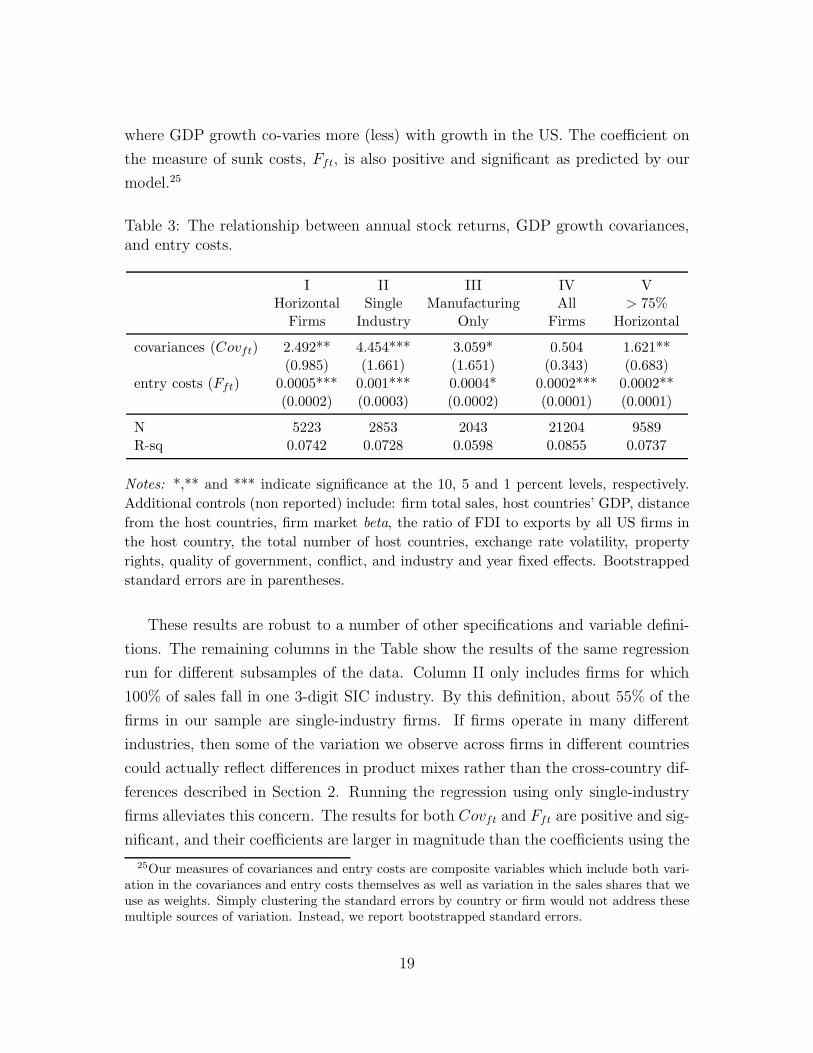
where GDP growth co-varies more (less) with growth in the US. The coefficient on

the measure of sunk costs, Fft, is also positive and significant as predicted by our

model.25

Table 3: The relationship between annual stock returns, GDP growth covariances,and entry costs.

I II III IV VHorizontal Single Manufacturing All > 75%

Firms Industry Only Firms Horizontal

covariances (Covft) 2.492** 4.454*** 3.059* 0.504 1.621**(0.985) (1.661) (1.651) (0.343) (0.683)

entry costs (Fft) 0.0005*** 0.001*** 0.0004* 0.0002*** 0.0002**(0.0002) (0.0003) (0.0002) (0.0001) (0.0001)

N 5223 2853 2043 21204 9589R-sq 0.0742 0.0728 0.0598 0.0855 0.0737

Notes: *,** and *** indicate significance at the 10, 5 and 1 percent levels, respectively.

Additional controls (non reported) include: firm total sales, host countries’ GDP, distance

from the host countries, firm market beta, the ratio of FDI to exports by all US firms in

the host country, the total number of host countries, exchange rate volatility, property

rights, quality of government, conflict, and industry and year fixed effects. Bootstrapped

standard errors are in parentheses.

These results are robust to a number of other specifications and variable defini-

tions. The remaining columns in the Table show the results of the same regression

run for different subsamples of the data. Column II only includes firms for which

100% of sales fall in one 3-digit SIC industry. By this definition, about 55% of the

firms in our sample are single-industry firms. If firms operate in many different

industries, then some of the variation we observe across firms in different countries

could actually reflect differences in product mixes rather than the cross-country dif-

ferences described in Section 2. Running the regression using only single-industry

firms alleviates this concern. The results for both Covft and Fft are positive and sig-

nificant, and their coefficients are larger in magnitude than the coefficients using the

25Our measures of covariances and entry costs are composite variables which include both vari-ation in the covariances and entry costs themselves as well as variation in the sales shares that weuse as weights. Simply clustering the standard errors by country or firm would not address thesemultiple sources of variation. Instead, we report bootstrapped standard errors.

19

full sample. The same concern about multi-product firms may also apply to firms

operating in different broad sectors, like wholesale, retail, or service firms. Thus the

specification in Column III includes only manufacturing firms. The coefficients are

positive for for both Covft and Fft, but they are only significant at the ten percent

level.26 Column IV includes all US MNCs, not just those that can be classified as

purely horizontal. The coefficient on Covft is not significant for this universe of

firms. This result is not surprising, as GDP shocks work through local demand in

our model and local demand is unlikely to impact vertical or export-platform FDI.

However, the sunk cost measure remains positive and significant. Finally, Column

V presents the results for a sample of “mostly horizontal” firms, where we use a

looser criterium to define a firm as horizontal: we define mostly horizontal firms

as those firms for which at least 75% of sales by foreign affiliates are to the local

market in which the affiliate resides. Using this definition, about 44% of the firms

in our sample can be classified as mostly horizontal MNCs. For this subsample, the

coefficients on covariances and entry costs are positive and significant.27

Our results confirm the importance of cross-country GDP growth covariances and

entry costs into the host countries for the stock returns of US multinationals. These

results provide a first pass of a theory built on those fundamentals, but disregard

the fact that – according to Eq. (10) – GDP growth correlations and entry costs

in the countries in which the firm does not have affiliates also matter, through the

option value term. In the next section we discuss our approach to controlling for

the components of the option value term by building proxies based on the estimated

probabilities that firms open affiliates in given countries.

4.2 Country Selection

Eq. (10) shows that GDP growth covariances and entry costs matter not only for

the value of assets in place, in the countries in which firms have affiliates, but also

for the option value of entering new countries. The difficulty in measuring the

contribution of these variables to the returns through the option value is that we

cannot construct firm-level measures like Eqs. (11) and (12) since firms do not have

26The full table of results broken down by sector is available upon request to the authors.27We also run our specification for the subsample of firms for which at least 50% of sales by

foreign affiliates are horizontal (70% of the firms in our sample). The results are qualitativelysimilar to the ones using all firms.

20

sales in these countries. However, we can estimate how likely it is that a firm will

enter a given country and then use these predicted probabilities to construct proxy

measures of the option value.

Our estimation of the likelihood of entering a country draws from the literature

on the determinants of FDI. According to the knowledge capital model developed

by Carr, Markusen, and Maskus (2001) and Markusen and Maskus (2002), the

volume of FDI activity between two countries depends on the sum of the GDPs of

the countries, the squared difference in their GDPs, the difference in skilled labor

endowments, and trade costs. The proximity-concentration model developed by

Brainard (1997) and Helpman, Melitz, and Yeaple (2004) suggests that a firm’s

decision to engage in FDI is a function of proximity, which we proxy with distance,

and market size, measured by the sum of US GDP and the GDP of the host country.

Data on these variables are compiled from several sources. Information regarding

real GDP and trade barriers come from the Penn World Tables. Trade costs are

measured using standard definitions of openness: 100 minus the trade share of

total GDP. Skill differences are measured using estimates of average educational

attainment by Barro and Lee (2010). We also include the sources of country risk

mentioned in Section 4.1 and described in detail in the appendix.

Another factor that likely impacts the future probability of entering a country

is the likelihood that the country will experience a large GDP shock in the future.

We proxy this likelihood using the dispersion of the country’s growth rate shocks.

When considering the likelihood of entering a new country, it is important to also

consider where the firm already has foreign affiliates. Work by Ekholm, Forslid, and

Markusen (2007) and Mrazova and Neary (2011) has demonstrated the importance

of export platform FDI, that is, firms choosing to use one foreign affiliate to serve

multiple countries rather than locating an affiliate in each country. This would

suggest that, under certain conditions, already having an affiliate in the same region

may reduce a firm’s incentives to enter a neighboring country. On the other hand,

Chen (2011) emphasizes the interdependence of location choices across affiliates of

the same MNC. She finds that the impact of already having a nearby affiliate can

be negative (in the case of export platform FDI) or positive, as is the case when

firms ship components between affiliates and thus benefit from proximity.

Even if our structural model does not allow for export platforms or intrafirm

trade in inputs, controlling for the presence of other affiliates in the region is impor-

21

tant empirically. In our country selection regression we include a dummy variable

that equals one if the firm had an affiliate in the region in year t − 1. To avoid

placing strong restrictions on what constitutes a region, we define regions broadly

as either Europe, Asia, NAFTA, Central and South America, Africa, and the Middle

East. The resulting estimating equation is:

Afjt = α + β1Wjt + β2Regionfj,t−1 + δt + εfjt (14)

where Afjt is a dummy variable that equals 1 if firm f has an affiliate in country

j in time t. Wjt is a vector of the knowledge capital, proximity-concentration and

country risk variables described above. Regionfj,t−1 is a dummy variable that equals

one if firm f had an affiliate in the region in which country j is located at time t−1.

We estimate Eq. (14) using both the full sample and the sample of purely horizontal

firms.

When considering the possible countries in which a firm may operate, we limited

the sample to the top 50 destination countries, which account for 96% of all foreign

activity by US firms. Table 4 shows the results of this probit regression. The

knowledge capital and proximity-concentration variables are significant predictors

of whether or not a given firm will have an affiliate in a given country. Although

none of the country risk measures are significantly related to the firm’s risk premium,

property rights protection and quality of government are positively and significantly

related to a firm’s decision to enter a given country. As expected, the coefficient on

armed conflict is negative, though not significant. The ratio of FDI sales to exports

at the country level is positive. As expected, GDP volatility is negatively related to

the decision to enter.

For each firm, we use these first step results to compute the predicted probability

of entering each country in which the firm does not currently have an affiliate. These

predicted entry probabilities are positively correlated with the actual rates of entry

that we observe in the sample, however there is still some noise at the firm level.

The correlation between actual new entry and our predicted probabilities at the firm

level is 0.10. The correlation is much higher at the country level: when we average

the predicted entry rate over all firms in each country, we get a correlation of 0.62

for the average predicted probability that any firm will enter the country and that

country’s actual number of new affiliate entrants.

22

Table 4: Probit regression of selection into FDI.

ALL FIRMS HORIZONTAL FIRMS

ln(distance) -0.126*** -0.159***(0.004) (0.007)

ln(sumgdp) 7.315*** 7.583***(0.179) (0.284)

ln(gdpdif2) 1.678*** 1.745***(0.059) (0.093)

ln(skilldif) 0.039*** 0.037***(0.004) (0.006)

ln(trade cost) -0.011*** -0.008***(0.001) (0.002)

st.dev.(GDP) -0.023*** -0.023***(0.002) (0.002)

st.dev.(exrate) -0.00004*** -0.00005***(0.000003) (0.000005)

property rights 0.004*** 0 004***(0.0002) (0.0004)

quality of gov. 0.100*** 0.236***(0.025) (0.039)

conflict -0.004 -0.001(0.003) (0.004)

FDI/export ratio 0.002*** 0.005**(0.001) (0.002)

Regionft−1 0.393*** 0.289***(0.005) (0.008)

Year FE YES YES

N 2769984 1355552Pseudo R-sq 0.1083 0.1171

Notes: ** and *** indicate significance at the 5 and 1 percent levels, respectively. Standard

errors clustered by country are in parentheses.

23

Using the results of the probit to proxy for the option value is consistent with

the model we developed in Section 2. According to the theory, the option value of a

firm in a foreign country is higher the likelier a firm is to enter a given country. In

the language of the model, a firm enters a country when its expected profits in that

country are above some threshold (that one can derive explicitly given functional

forms for preferences and technologies, see Appendix A). The estimated probability

of entering a country that results from the probit can then be interpreted as a

measure of how close a firm is to the entry threshold and hence of how important

the option value of entering that country is.

To understand the option value of entry, we next construct a weighted average

of the GDP growth covariances between the US and the countries in which the firm

does not have affiliates, using the predicted probabilities as weights:

Covoft =

∑

j 6∈A

probfjtCovj

∑

j 6∈A

probfjt(15)

where probfjt is the predicted probability that firm f has an affiliate in country j

in time t from the first step estimation and Covj is the covariance of GDP growth

between the US and country j. We construct a similar measure for the cost of capital

required to start a business in the countries in which the firm does not currently

have affiliates.

Table 5: Summary statistics by affiliate presence.

Covariance Entry cost ($)

ALL FIRMS

Countries with affiliates 2.718 4007.04Countries without affiliates 2.319 7057.54

HORIZONTAL FIRMS

Countries with affiliates 2.725 2559.17Countries without affiliates 2.384 6938.89

Table 5 shows the weighted average GDP growth covariances and cost of capital

24

required to start a business for the countries in which a firm does and does not have

affiliates. For the average horizontal firm in our sample, the GDP growth covariance

for countries in which the firm has affiliates is 2.725. The weighted covariance of

shocks for countries in which they do not have affiliates is 2.384. These numbers

suggest that US MNCs don’t choose their affiliates’ host countries with the only

purpose of to diversifying away risk. If this were the case, we would observe them

self-selecting into countries whose GDP growth co-varies less with the US GDP

growth. The weighted cost of capital required to start a business in the countries

where the firms have affiliates is $2,559. For countries in which they do not have

affiliates, that cost is $6,939. These numbers indicate that US MNCs privilege

locations with lower entry costs. The same patterns hold for the full sample of

firms.

Appendix B includes a table showing the reduced form results controlling for

characteristics of the countries in which each firm does not have affiliates. The

effects of GDP growth covariances and of the sunk cost measures are qualitatively

and quantitatively similar to the results from Table 3. The effect of the GDP growth

covariances and entry costs on the returns via the option value component should

have the same sign as the effect of these forces through the component measuring

assets in place. This is true for the covariances Covoft, which exhibit a positive, albeit

non significant coefficient in the baseline specification, but not for the sunk costs,

F oft, whose coefficient is negative and significant. The robustness of our reduced

form results to the inclusion of these option value proxies is reassuring. However,

in order to get better estimates of the option values themselves, we now turn to

specifications that are more closely related to the model presented in Section 2.

4.3 Model-Based Estimates

The reduced form regressions we presented above confirm the presence of a statistical

relationship between GDP growth covariances, sunk and fixed costs of production

and the stock returns of multinational corporations. We now move to a more struc-

tural approach, which is derived closely from the theoretical relationship that the

model delivers, Eq. (10). The model-based analysis presented here allows us to

accomplish two tasks. First, we are able to decompose the risk premium into the

separate contributions of individual host countries. Second, we are able to quantify

25

the contribution of assets in place versus option value to the risk premium.

We can re-write Eq. (10) as:

E(retf )− rh = γ

[

σ2hε

fh +

∑

j∈A

σhσjρjεfj +

∑

j 6∈A

σhσjρjεofj

]

(16)

where εfh ≡ YhV′hY /V is the elasticity of the firm’s value with respect to GDP in

the home country, εfj ≡ YjV′jY /V is the elasticity of the firm’s value with respect

to GDP in host country j ∈ A, and εofj ≡ YjVoj′

Y/V is the elasticity of the firm’s

option value with respect to GDP in a potential host country j 6∈ A. The term

σ2hε

fh captures firm f ’s domestic risk exposure. The term

∑

j∈A σhσjρjεfj captures

the risk exposure arising from the foreign countries where firm f has affiliates. The

term∑

j 6∈A σhσjρjεofj captures the risk exposure arising from the countries where

firm f does not currently operates (the option value).

In order to run a regression based on Eq. (16), we need to compute the elasticities

εfh, εfj for j ∈ A, and εofj for j 6∈ A. Since the value of the firm in the countries

where it has affiliates is not observable, we proxy it with the firm’s net income

in country j, Ifjt.28 Net income exhibits a substantial amount of variation across

countries and firms. Since income is an imperfect measure of the value of the firm,

we assume that the true elasticity εfj is given by the approximated elasticity εfj times

a country-specific unobserved component ζj:

εfj ≡ ζj εfj . (17)

The approximated elasticity εfj is estimated by running one time series regression

of log-income on log-GDP for each firm f and host country j:29 ln(Ifjt) = α +

28Net income is given by the firm’s income from sales and investment minus total costs andexpenses, so it is a measure of the firm’s affiliate profits in country j. This measure, like flowprofits at the affiliate level (which are not available from the BEA data), is not a perfect measureof the value of the firm because it disregards the option value of assets in place. Alternatively,CRSP contains data on profits and market capitalization at the firm level. This measure is alsoproblematic as we only have information on the firm total market capitalization and total profits,not by individual affiliate or country of operation, hence the variation of εfj across countries only

comes from variation in Yjt. To construct εfj , we also need to take a stand on the status of MNCsthat enter or exit countries during the sample period. In our baseline specification, we consider theeffect on the returns of those assets that are in place for at least two years of the sample period.

29When we regress log net income on log gdp, observations with negative net income are dropped,

26

εfj ln(GDPjt). We estimate εfh in the same way, regressing the log of each firm’s

domestic net income on the log of US GDP.

The terms ζh, ζj for j ∈ A, account for country-specific factors that impact the

value of firms in each country and are not captured by net income. Income changes

are primarily driven by shocks to local demand, however value has much broader de-

terminants, including the expectation about future cash-flows. For example, shocks

to expectations about institutional quality, rule of law, taxes, or political factors

may impact the valuation of firms in a country without necessarily being reflected

in their income.

Estimating the elasticity εfj using actual data on the responsiveness of each firm’s

income to local GDP shocks also helps us avoid potential complications resulting

from differences between horizontal, vertical, and export platform FDI. GDP growth

shocks in host countries impact US MNCs through local demand, which should have

a greater effect on firms that rely more heavily on sales to the local market. For

our reduced form approach, we addressed the distinction between horizontal versus

vertical sales by only including purely horizontal firms in our analysis. However,

this distinction is not an issue in our model-based estimation. Here we are able to

directly identify the responsiveness of the net income of each firm to fluctuations

in the local market using the estimates of εfj . By estimating this elasticity directly

at the firm level, we pick up any differences in responsiveness to local GDP across

firms that may result from being primarily horizontal or vertical in structure.

We also prefer to avoid making a strong distinction between horizontal versus

vertical FDI in these estimates because most firms do not fall cleanly into one of

those two categories. The majority of US MNCs engage in some combination of

both horizontal and vertical FDI, but most of the sales by US MNCs are horizontal.

For example, in our sample, 64% of sales by foreign affiliates of US firms are to the

generating selection bias in our estimates. An alternative would be to approximate the elasticitiesas:

εfj ≈

T∑

t=1

[

(Ifjt − Ifj,t−1)/Ifj,t−1

(GDPjt −GDPj,t−1)/GDPj,t−1

]

·1

T

where Ifjt denotes the net income of firm f in country j in year t, and GDPjt denotes the GDP ofcountry j in year t. This method allows us to compute the elasticities for all the firm-country pairin the sample, but – as an approximation – is affected by measurement error. We run our model-based estimation also using the alternative specification above, and the results are qualitativelysimilar.

27

market in which the affiliate is located and 94% of the firms have at least some sales

to the local markets in which their affiliates are located. Thus for our full sample of

firms, almost all of them have at least some sales to the local market, and for most

affiliates these local sales make up the majority of their total sales. The structural

estimates that follow make use of the full sample of firms, rather than focusing on

firms that only have horizontal sales.

Next, in order to estimate the full Eq. (16), we need to construct a proxy for the

elasticity of the option value of the firm: εofj ≡YjV

oj

′

Y

V. We cannot proxy this elasticity

using foreign income measures since firms don’t have income in the countries where

they don’t have affiliates. We proxy it instead as εofj ≈ ζoj probfj ε

fh, where ε

fh is the

firm’s elasticity of domestic net income with respect to GDP fluctuations in the US.

This measure captures the firm-specific component of elasticity, and does not suffer

from bias due to selection into affiliate countries, as it is a purely domestic measure.

probfj is the predicted probability that firm f will enter country j, as estimated in

Section 4.2. By multiplying the domestic elasticity by the estimated probability, we

assign higher responsiveness to shocks to those firms that are more likely to enter

a foreign market, and for which the model predicts the option value to be more

important. The term ζoj accounts for other country-specific factors that may impact

the value of firms in potential host country j.30

This leads to the following estimation equation:

E(retf )− rh = ψhσ2hε

fh +

∑

j∈A

ψjσhσjρj εfj +

∑

j 6∈A

ψojσhσjρjprob

fj ε

fh + νf (18)

where ψh ≡ γζh, ψj ≡ γζj, ψoj ≡ γζoj .

We present the results in two parts. First, we decompose the risk premium of

the firm into the contributions of each individual host country. Next, we aggregate

the risk premia across countries to give an estimate of total MNCs’ risk. Each of

these sets of results is further decomposed into the contributions of assets in place

and option value.

30Our approximation of the elasticity of the option value is justified by the theoretical model,which – under appropriate functional assumptions – implies that the elasticity of the option valueis the product of a potential host country-specific component and of a firm-country-specific com-ponent that is increasing in firm productivity and in the likelihood that the firm will enter thatspecific country. See Appendix A for details about how to map the model into our approximationin the data.

28

4.3.1 Decomposition of Risk Premium by Country

In this section we use the entire sample of firms having affiliates in the top 50 coun-

tries to estimate Eq. (18). We begin by estimating Eq. (18) without controlling for

the option value. We do this by introducing a separate variable for each host coun-

try j which takes value σhσjρj εfj if firm f has an affiliate in country j and equals

zero if firm f does not have an affiliate in country j. It is worth noting that we do

not identify the estimated coefficient ψj as the risk price (or risk aversion) because

it contains the country specific non-observed component of the firms’ elasticity of

value with respect to GDP. Since the relationship in Eq. (18) should hold within in-

dustries, we add industry fixed effects to the specification. The results are reported

in Table 6 under specification I.31 In the left panel we report the estimated coeffi-

cients ψj , while in the right panel we report the corresponding average risk premia

ψjσhσjρj εfj . For clarity of exposition, Table 6 only reports the risk premia for ψj co-

efficients that are either statistically significant or that correspond to a country that

is an especially important FDI destination for US firms, such as the UK, Mexico,

and China. We report the full set of results for all countries in Appendix B.

As Table 6 shows, 12 of the ψj coefficients are statistically significant at least

at the ten percent level in at least one of our specifications. Of these 12 significant

coefficients, 10 are associated with a positive risk premium (ψjσhσjρj εfj > 0), in-

dicating that the corresponding host countries are a source of risk to MNCs with

affiliates there. The countries with the highest risk premia are Greece, Malaysia,

Singapore, Denmark, India, and China. Most European countries and Canada have

relatively low risk premia, indicating that the effect of low sunk costs outweighs the

one of high co-movement with the US.

Each country-specific risk premium can be interpreted as the additional annual

return required to induce investors to hold shares of firms with affiliates in that

country. For example, firms with affiliates in Greece have annual returns that are,

on average, 0.54 percentage points higher than those of firms that do not have

affiliates in Greece. For firms that have affiliates in the UK, the additional annual

return is only 0.02 percentage points.

The country-specific risk premia reported here are for the average firm in our

31Since the firm-level elasticities εfj are generated regressors, we report bootstrapped standarderrors.

29

Table 6: Country-specific estimates of risk premia, observations at the firm-yearlevel.

coefficients risk premia

I II I II

ψj ψj ψoj ψjσhσjρj εj

f ψjσhσjρj εjf ψo

jσhσjρjprobfj εh

f

US Domestic 0.036*** 0.047*** 0.2302 0.3005(0.007) (0.013)

Canada 0.030*** 0.030*** 0.7091 0.1209 0.1209 0.0953(0.011) (0.011) (0.531)

Mexico 0.0534 0.060* 0.4184 0.1888 0.2123 0.0231(0.036) (0.036) (1.018)

Denmark 0.162*** 0.163*** -0.4970 0.3977 0.4001 -0.0238(0.052) (0.052) (2.201)

Germany -0.0089 -0.0081 1.492* -0.0158 -0.0144 0.1475(0.006) (0.006) (0.886)

Greece 0.314*** 0.306** -0.3356 0.5582 0.5440 -0.0072(0.144) (0.144) (5.150)

Ireland 0.0015 0.004* -1.455* 0.0207 0.0555 -0.3290(0.002) (0.002) (0.803)

Netherlands 0.028** 0.025** 0.2572 0.1355 0.1210 0.0293(0.011) (0.011) (1.018)

United Kingdom 0.0046 0.0043 1.4119 0.0253 0.0236 0.3366(0.008) (0.008) (0.428)

Israel -0.572** -0.524** -32.222*** -0.6913 -0.6333 -0.2115(0.222) (0.223) (10.394)

Australia 0.089* 0.080* -3.1719 0.1438 0.1293 -0.0580(0.050) (0.050) (3.188)

Indonesia 0.075* 0.0655 14.1327 -0.0731 -0.0639 -0.0504(0.046) (0.047) (13.861)

Japan 0.011** 0.011** -0.1613 0.0110 0.0110 -0.0053(0.006) (0.006) (0.672)

Malaysia 0.244*** 0.228*** -0.9948 0.5780 0.5401 -0.0177(0.086) (0.087) (5.368)

Singapore 0.070*** 0.062*** -1.1673 0.4580 0.4057 -0.0785(0.018) (0.019) (1.570)

China 0.5649 0.5217 1.0715 0.2427 0.2242 0.0069(0.578) (0.584) (8.350)

Notes: *,** and *** indicate significance at the 10, 5 and 1 percent levels. Both specifications

include industry and year fixed effects and have N=25536. Bootstrapped standard errors are in

parentheses.

30

sample. However, firms are very heterogeneous in terms of their responsiveness to

shocks. This heterogeneity enters through εfj , the elasticity of the firm’s value with

respect to changes in host country GDP. Thus the positive values for the country-

level risk premia indicate that firms whose values are more responsive to changes in

destination countries’ GDP tend to be riskier and to exhibit higher returns.

As mentioned above, the results of specification I do not take into account the

contribution to the risk premium of potential host countries (the option value).

This results in biased estimates of the risk premia. To address this concern, in

specification II we report the results of regression (18) including the controls for

the option value countries. As long as our proxy for the option value is a good

one, controlling for the option value term corrects the omitted variable bias in the

estimated coefficients on assets in place, ψj . Moreover, the difference between the

R2 in the two specifications quantifies how much more of the variance of the risk

premium is explained by explicitly taking into account the option value of entering

new countries using the approximation described above.

For the majority of the countries that had a positive risk premium in specification

I, adding the control for the option value decreases the estimated risk premium. This

suggests that attempting to estimate the risk premium without controlling for the

option value overestimates the risk premium. Figure 1 plots the estimated country-

level contributions to the risk premium. To keep the graph legible, we’ve only

labeled data points for the highest and lowest risk countries, as well as for the most

important FDI destination countries.

In addition to their role in resolving the omitted variable bias, the option value

terms are also informative themselves. In the entire sample of top 50 countries,

there are 14 for which the ψoj coefficient is significant; of those, 6 are associated with

a positive risk premium, indicating that the mere possibility of a firm entering those

countries is a source of risk to investors. The coefficients on the option value terms

vary much more widely than the coefficients on the the assets in place. This is not

surprising, as the approximated firm-level elasticities for the option value countries

are not as good of an approximation of the true elasticity as in the case of assets

in place. The corresponding risk premia (ψojσhσjρjprob

fj ε

fh) are still reasonable in

magnitude, ranging from -0.38 to 0.54.

Finally, F-tests (not reported here) show that all the estimated parameters ψj

and ψoj are significantly different from each other. This result confirms the impor-

31

Greece

Malaysia

Singapore

India

China

Mexico

Norway

France

Germany

Switzerland

Japan

UK

Canada

NetherlandsIreland

−.2

0.2

.4.6

risk

prem

ium

, con

trol

ling

for

optio

n va

lue

0 10 20 30 40 50rank

Figure 1: Estimated Country-Specific Risk Premia.

tance of heterogeneity across-countries in the unobserved component of the elasticity

of firms’ value with respect to GDP.

−20

020

40ac

tual

ann

ual r

etur

n

−20 0 20 40predicted annual return, controlling for option value

Figure 2: Predicted versus realized returns. Predicted returns include the optionvalue of entering new countries.

We conclude this section with a graphical representation of the model fit control-

ling for the option value of entering new countries. Figure 2 plots realized returns

32

Table 7: Aggregate risk premia.

I II

Risk premium:- from domestic sales: 0.230 0.301- from foreign sales: 3.014 3.003- from option value: 0.651

against returns predicted by the model, corresponding to the full specification II.32

The plot gives a graphical representation of the fit of the model. Overall, the esti-

mated stock returns do a good job of matching the actual returns.

4.3.2 Aggregate Risk Premium

The results presented in Table 6 shed light on the magnitude of country-level risk

premia. However, we are also interested in their aggregation to the overall risk

premium of multinational firms, most of which have affiliates in more than one

country.

To estimate the aggregate risk premium we sum the country-specific risk premia

reported in Table 6. Table 7 shows the results. The aggregate risk premium from

foreign assets in place is large, at about 3 percentage points. By summing over

the risk premia for all countries, we are constructing an estimate of what the risk

premium would be for a firm that has affiliates in all of the top 50 FDI host countries.

This implies that a firm with affiliates in every country in our sample would have, on

average, expected annual returns that are 3% higher than those of a purely domestic

firm.33

As was the case for most of the country-level risk premia, the aggregate risk

premium from assets in place falls slightly when the option value term is included.

The aggregate risk premium of the option value implies that, for a firm that does

not have affiliates in any of the countries in our sample, the option to enter all the

32To construct the plots, we divided the observations into bins based on their predicted annualreturns from regression (18). Each bin is 0.5 units wide, resulting in about 70 bins. Then weaveraged actual and predicted annual returns within these bins and graphed those averages.

33As mentioned above, these results hinge on the assumption that firms take the decision ofentering a country independently of their presence in other countries.

33

potential host countries in the future increases expected returns by 0.651% for the

average firm.

As mentioned above, the aggregate results give the risk premium for an average

firm with affiliates in all of the countries in the sample. However, it is also possible to

use the country-specific results from Table 6 to estimate the expected risk premium

for a typical firm with any combination of foreign affiliates. For example, suppose

that a firm only has affiliates in Canada, Singapore, and Ireland. The expected

contribution of these assets in place to the firm’s risk premium would be 0.1209 +

0.4057+0.0555 = 0.582. The contribution to the risk premium from the option value

of entering countries in which the firm does not currently have affiliates would be the

sum∑

j 6∈A ψojσhσjρjprob

fj ε

fh where j 6∈ A includes all countries except for Canada,

Singapore, and Ireland. This is a value of 0.963. Adding in the risk premium for

domestic US assets, the total risk premium for the average firm with affiliates in

Canada, Singapore, and Ireland would be 0.301 + 0.582 + 0.963 = 1.846, so the

expected returns would be almost 2 percentage points higher than the returns of a

purely domestic firm.

5 Conclusions

In this paper we study theoretically and empirically the cross-section of returns of

multinational corporations, to establish a link between the geographic structure of

a firm and its risk premium. Stock returns are impacted by firms’ diversification of

country-level risk, which makes firms safer and decreases returns, and by the fixed

and sunk costs associated with investing abroad, which make firms more leveraged,

hence riskier, and increase returns. We test the predictions of the model using firm

level data on multinational corporations from the US BEA merged with firm level

stock return data from CRSP. The empirical results support the model’s predictions.

MNCs with affiliates in countries where shocks co-move more with the home country

and where entry costs are higher tend to have higher risk premia. We use the

structural model to decompose firm-level risk premia into individual host countries’

contributions and to assess the relative importance of assets in place versus option

value for the returns.

This paper plays an important role in understanding the complex interactions

34

between MNCs and financial markets. There are a number of additional questions

that this analysis leaves aside. Are there systematic patterns in the expansion

strategies of MNCs across host countries over time? Are entry and exit episodes

associated with sizable changes in the stock market valuation of firms? What is

the relevant time horizon to study MNCs’ expansion across countries and the cor-

responding stock market responses? These are interesting avenues that we plan to

pursue in future work.

References

Alfaro, Laura, and Maggie X. Chen. 2013. “The Global Agglomeration of Multi-

national Firms.” NBER working paper 15576.

Atkeson, Andrew, and Tamim Bayoumi. 1993. “Do private capital markets insure

regional risk? Evidence from the United States and Europe.” Open Economies

Review 4:303–324.

Baker, Malcolm, C. Fritz Foley, and Jeffrey Wurgler. 2009. “Multinationals as

Arbitrageurs? The Effect of Stock Market Valuations on Foreign Direct Invest-

ment.” Review of Financial Studies 22 (1): 337–369.

Barro, Robert J., and Jong-Wha Lee. 2010. “A new data set of educational

attainment in the world, 1950-2010.” NBER working paper 15902.

Brainard, S. Lael. 1997. “An Empirical Assessment of the Proximity-Concentration

Trade-off between Multinational Sales and Trade.” The American Economic

Review 87 (4): 520–544.

Branstetter, Lee G., Raymond Fisman, and C. Fritz Foley. 2006. “Do Stronger

Intellectual Property Rights Increase International Technology Transfer? Em-

pirical Evidence from U.S. Firm-Level Panel Data.” Quarterly Journal of Eco-

nomics 121 (1): 321349.

Carr, David L, James R. Markusen, and Keith E. Maskus. 2001. “Testing the

knowledge-capital model of the multinational enterprise.” American Economic

Review 91 (3): 995–1001.

Caselli, Francesco, Miklos Koren, Milan Lisicky, and Silvana Tenreyro. 2014. “Di-

versification through Trade.” Mimeo, London School of Economics.

35

Chen, Maggie X. 2011. “Interdependence in Multinational Production Networks.”

Canadian Journal of Economics 44 (3): 930–956.

Chen, Maggie X., and Michael Moore. 2010. “Location Decision of Heterogeneous

Multinational Firms.” Journal of International Economics 80 (2): 188–199.

Crucini, Mario. 1999. “On international and national dimensions of risk sharing.”

Review of Economics and Statistics 8 (1): 73–84.

Das, Sanghamitra, Mark J. Roberts, and James R. Tybout. 2007. “Market Entry

Costs, Producer Heterogeneity, and Export Dynamics.” Econometrica 75 (3):

837–873.

Denis, David J., Diane K. Denis, and Keven Yost. 2002. “Global Diversification,

Industrial Diversification, and Firm Value.” The Journal of Finance 57 (5):

1951–1979.

Dixit, Avinash K. 1989. “Entry and Exit Decisions under Uncertainty.” Journal

of Political Economy 97 (3): 620–638.

Dixit, Avinash K., and Robert S. Pindyck. 1994. Investment under Uncertainty.

Princeton, NJ: Princeton University Press.

Ekholm, Karolina, Rikard Forslid, and James R. Markusen. 2007. “Export-

Platform Foreign Direct Investment.” Journal of the European Economic As-

sociation 5 (4): 776–795.

Fama, Eugene F., and Kenneth R. French. 1996. “Multifactor Explanations of

Asset Pricing Anomalies.” Journal of Finance 51 (1): 55–84.

Fillat, Jose L., and Stefania Garetto. 2014. “Risk, Returns, and Multinational

Production.” Mimeo, Boston University.

Hall, Robert E. 1978. “Stochastic Implications of the Life Cycle-Permanent Income

Hypothesis: Theory and Evidence.” Journal of Political Economy 86 (6): 971–

987.

Head, Keith, Thierry Mayer, and Joh Ries. 2010. “The erosion of colonial trade

linkages after independence.” Journal of International Economics 81 (1): 1–14.

Helpman, Elhanan, Marc J. Melitz, and Stephen R. Yeaple. 2004. “Exports Versus

FDI with Heterogeneous Firms.” The American Economic Review 94 (1): 300–

316.

36

Inoue, Atsushi, and Gary Solon. 2010. “Two-Sample Instrumental Variables Esti-

mators.” The Review of Economics and Statistics 92 (3): 557561.

Jacquillat, Bertrand, and Bruno Solnik. 1978. “Multinationals are poor tools for

international diversification.” Journal of Portfolio Management 4 (2): 812.

Kravis, Irving B., and Robert E. Lipsey. 1982. “The location of overseas pro-

duction and production for export by U.S. multinational firms.” Journal of

International Economics 12 (3-4): 201–223.

Markusen, James R., and Keith E. Maskus. 2002. “Discriminating among al-

ternative theories of the multinational enterprise.” Review of International

Economics 10:694–707.

Mrazova, Monika, and J. Peter Neary. 2011. “Firm Selection into Export-Platform

Foreign Direct Investment.” Working paper.

Ramondo, Natalia, Veronica Rappoport, and Kim J. Ruhl. 2013. “The Proximity-

Concentration Tradeoff under Uncertainty.” Review of Economic Studies 80

(4): 1582–1621.

Roberts, Mark J., and James R. Tybout. 1997. “The Decision to Export in

Colombia: An Empirical Model of Entry with Sunk Costs.” The American

Economic Review 87 (4): 545–564.

Rowland, Patrick F., and Linda L. Tesar. 2004. “Multinationals and the gains

from international diversification.” Review of Economic Dynamics 7:798–826.

Senchack, Andrew J., and William L. Beedles. 1980. “Is indirect international

diversification desirable?” Journal of Portfolio Management 6 (2): 49–57.

Sorensen, Bent E., and Oved Yosha. 1998. “International risk sharing and Euro-

pean monetary unification.” Journal of International Economics 45:211–238.

Teorell, Jan, Nicholas Charron, Stefan Dahlberg, Sren Holmberg, Bo Rothstein,

Petrus Sundin, and Richard Svensson. 2013. “The Quality of Government

Dataset.” University of Gothenburg: The Quality of Government Institute,

http://www.qog.pol.gu.se.

Tesar, Linda L., and Ingrid Werner. 1998. “The internationalization of securi-

ties markets since the 1987 crash.” In R. Litan and A. Santomero (eds.) ,

37

Brookings-Wharton Papers on Financial Services. Washington: The Brookings

Institution.

Yeaple, Stephen. 2003. “The Complex Integration Strategies of Multinational

Firms and Cross-Country Dependencies in the Structure of Foreign Direct In-

vestment.” Journal of International Economics 60 (2): 293–314.

. 2009. “Firm Heterogeneity and the Structure of U.S. Multinational Ac-

tivity: An Empirical Analysis.” Journal of International Economics 78 (2):

206–215.

38

Appendix

A Derivation of the Model

We present here the derivation of the results contained in Section 2. In the contin-

uation region, each one of the three components of the value function of a firm (Vh,

Vj, and Voj ) satisfies:

π(a, Y,X)M∆t + E[M∆t · V (a, Y ′, X|Y )]− V (a, Y,X) = 0. (B.1)

For ∆t→ 0:

π(a, Y,X)Mdt+ E[d(M · V (a, Y,X))] = 0. (B.2)

The term in the expectation can be written as:

E[d(M · V )] = E[dM · V +M · dV + dM · dV ]

= M · V · E

[dM

M+dV

V+dM

M·dV

V

]

= M · V

[

−rdt + E

(dV

V

)

+ E

(dM

M·dV

V

)]

= Mdt

[

−rV + E

(dV

dt

)

+ E

(dM

M·dV

dt

)]

(B.3)

where the dependence of V on (a, Y,X) has been suppressed to ease the notation.

Plugging Eq. (B.3) into Eq. (B.2):

π − rV + E

(dV

dt

)

+ E

(dM

M·dV

dt

)

= 0. (B.4)

By applying Ito’s Lemma and using the expressions for the Brownian motions

ruling the evolution of Y , we can derive expressions for some of the terms in Eq.

(B.4):

dV = V ′Y dY +

1

2σ2Y 2V ′′

Y dt = V ′Y [µY dt+ σY dz] +

1

2σ2Y 2V ′′

Y dt

E[dV ] = µY V ′Y dt +

1

2σ2Y 2V ′′

Y dt .

Using these results and the equation describing the evolution of M , we can

39

rewrite Eq. (B.4) for the three value functions as:

πhdt− rhVhdt+ µhYhVh′Y dt+

1

2σ2hY

2h Vh

′′Y dt+ ...

...E

[

(−rhdt− γσhdzh) ·

(

µhYhVh′Y dt+ σhYhVh

′Y dzh +

1

2σ2hY

2h Vh

′′Y dt

)]

= 0.

πjdt− rhVjdt+ µjYjVj′Ydt+

1

2σ2jY

2j Vj

′′Ydt+ ...

...E

[

(−rhdt− γσhdzh) ·

(

µjYjVj′Y dt+ σjYjVj

′Y dzj +

1

2σ2jY

2j Vj

′′Y dt

)]

= 0.

−rhVoj dt+ µjYjV

oj′

Ydt+

1

2σ2jY

2j V

oj′′

Ydt+ ...

...E

[

(−rhdt− γσhdzh) ·

(

µjYjVoj′

Ydt+ σjYjV

oj′

Ydzj +

1

2σ2jY

2j V

oj′′

Ydt

)]

= 0.

The terms in expectations can be reduced to:

E

[

(−rhdt− γσhdzh) ·

(

µhYhVh′Y dt+ σhYhVh

′Y dzh +

1

2σ2hY

2h Vh

′′Y dt

)]

= ...

...− γσ2hY Vh

′Y dt

E

[

(−rhdt− γσhdzh) ·

(

µjYjVj′Ydt+ σjYjVj

′Ydzj +

1

2σ2jY

2j Vj

′′Ydt

)]

= ...

...− γρjσhσjY Vj′Ydt

E

[

(−rhdt− γσhdzh) ·

(

µjYjVoj′

Ydt+ σjYjV

oj′

Ydzj +

1

2σ2jY

2j V

oj′′

Ydt

)]

= ...

...− γρjσhσjY Voj′

Ydt.

So we obtain the no-arbitrage conditions (7)-(9) in the paper:

πh − rhVh + (µh − γσ2h)YhVh

′Y +

1

2σ2hY

2h Vh

′′Y = 0

πj − rhVj + (µj − γρjσhσj)YjVj′Y+

1

2σ2jY

2j Vj

′′Y

= 0

−rhVoj + (µj − γρjσhσj)YjV

oj′

Y+

1

2σ2jY

2j V

oj′′

Y= 0.

To derive the expression for the returns that guides our empirical analysis (Eq.

40

(10)), we combine the three equations above to obtain:

πh − rhVh − γσ2hYhVh

′Y + µhYhVh

′Y +

1

2σ2hY

2h Vh

′′Y

︸ ︷︷ ︸

E(dVh)

+...

∑

j∈A

πj − rhVj − γρjσhσjYjVj′Y+ µjYjVj

′Y+

1

2σ2jY

2j Vj

′′Y

︸ ︷︷ ︸

E(dVj)

+...

+∑

j 6∈A

−rhV

oj − γρjσhσj)YjV

oj′

Y+ µjYjV

oj′

Y+

1

2σ2jY

2j V

oj′′

Y︸ ︷︷ ︸

E(dV oj )

= 0.

Since E(dVh) +∑

j∈A

E(dVj) +∑

j 6∈A

E(dV oj ) = E(dV):

πh +∑

j∈A

πj + E(dV) = rhVh + γσ2hYhVh

′Y +

∑

j∈A

(rhVj + γρjσhσjYjVj

′Y

)+ ...

...∑

j 6∈A

(

rhVoj + γρjσhσjYjV

oj′

Y

)

πh +∑

j∈A

πj + E(dV)

V= rh + γ

σ2hYhVh

′Y +

∑

j∈A

σhσjρjYjVj′Y+∑

j 6∈A

σhσjρjYjVoj′

Y

V

.

To gain additional insight on the components of this expression, we can solve

explicitly each no-arbitrage condition to deliver quasi-closed form solutions for the

components of a firm’s value function. For illustration purposes, assume that profits

πj are a linear affine function of Yj (as it would be under linear cost functions and

CES demand): πj(a, Yj, Xj) = δj(a,Xj)Yj − fj where δj(a,Xj) denotes variable

profits as a share of GDP in country j and fj denotes the fixed costs of production

in country j. Then we can solve explicitly Eqs. (7)-(9) in the paper to obtain:

Vh =δh(a,Xh)Yhrh − µh + γσ2

h

−fhrh

(B.5)

Vj =δj(a,Xj)Yj

rh − µj + γρjσhσj−fjrh

+ cj(a,Xj)Yαj (B.6)

V oj = coj(a,Xj)Y

βj (B.7)

41

where α < 0 and β > 1 are known combinations of aggregate parameters and

cj(a,Xj) and coj(a,Xj) are firm-specific, positive magnitudes that can be determined

by imposing value-matching and smooth pasting conditions linking Eqs. (B.6) and

(B.7) for each country j, like in Dixit (1989). Hence the elasticity of assets in place

in country j is:

YjVj′Y

V=

δj(a,Xj )Yj

rh−µj+γρjσhσj+ αcj(a,Xj)Y

αj

V(B.8)

and the elasticity of the option value of entering country j is:

YjVoj′

Y

V=βcoj(a,Xj)Y

βj

V. (B.9)

Eqs. (B.8)-(B.9) illustrate that the elasticity of the value of assets in place in a

country is different from the elasticity of the option value in that country. Since

both profits and the magnitudes cj(a,Xj), coj(a,Xj) are firm-specific, the elasticities

also differ across firms.

The processes for the elasticities that we estimate in our model-based empirical

analysis are meant to mimic the variation that Eqs. (B.8)-(B.9) imply. For the

elasticity of assets in place, having information on firm’s income in each host country

j ∈ A allows us to approximate the elasticity directly. The approximation of the

elasticity of the option value is more indirect. It can be shown that the magnitude

coj(a,Xj) is increasing in firm’s productivity, indicating that more productive firms

have a higher likelihood to enter a country. In the empirical specification, this

higher likelihood to enter is expressed by probfj , which is the estimated probability

that firm f will enter country j given the country characteristics included in the

probit specification (Xj). However, the only firm-level characteristic included among

the regressors of the probit is the previous presence in a region. This is clearly

not enough to incorporate all the firm-level variation embodied incoj (a,Xj)

V, so we

multiply the estimated probability by the domestic elasticity to capture the firm-

specific components of the elasticity of the option value without suffering from the

potential bias due to selection into affiliate countries that one would introduce using

not purely domestic measures. Finally, the aggregate, host country-specific term

βY βj is captured by the estimated unobserved component ζoj .

42

B Robustness: Reduced Form Estimates

In this section we include a number of robustness tests to ensure that our empirical

results are not sensitive to changes in variable definitions or controls. We begin by

reporting the full set of results presented in Table 3 with all controls included. Next

we repeat our preferred specification controlling for a variety of other factors related

to size that may impact stock returns beyond total firm sales. These are market

capitalization, leverage, and the book-to-market ratio of the firm. We then replace

our measure of country-specific entry costs with two alternative measures from the

World Bank’s Doing Business Database: the number of procedures required to start

a business and the average number of days required to start a business. We also

present the results using a different methods to construct the firm-level sunk cost

measure, using affiliates counts as weights in Eq. (12). Finally, we measure the co-

movement of GDP shocks in the US and the host countries using the correlations,

rather than the covariances, of these shocks. Since our reduced form specification

does not control for the option value of opening new affiliates, we then report the

results of the second-step regressions including measures of the option value term

that we constructed using the results of the dynamic selection equation in Section

4.2. We conclude by reporting the entire set of results of our model-based estimation.

Table B.2 reports the complete results of the specifications that we summarized

in Table 3 in the paper. Our measure of firm size is total firm sales from the

BEA data. Gravity variables for the affiliates’ host countries come from CEPII (see

Head, Mayer, and Ries (2010)) and are aggregated at the firm level following the

same aggregation method as in Eq. (12). To control for the potential bias induced

by the fact that neither our model nor our empirical analysis incorporate exports,

we include an aggregate country-level measure of the ratio of total FDI sales by US

firms over total US exports for each country. In addition to these, we add other

sources of country risk as controls. Exchange rate volatility may be another source

of country-level risk, hence we control for the standard deviation of the country’s

exchange rate with respect to the US dollar over the sample period. Finally, we use

measures of rule of law, property rights, and conflict form the Quality of Government

Dataset. This dataset was compiled by Teorell et al. (2013) using information from

various different sources. These include the PRS Group’s International Country

Risk Guide (ICRG) indicator of quality of government, which we use to proxy for

43

Table B.1: Summary Statistics of Robustness Controls.

N. Obs Mean Std. Dev. Min Max

ALL FIRMS

GDP 21809 1070.237 743.855 0 5333.925distance 21809 5860.26 3057.661 0 16370.82firm beta 21809 0.920885 1.128112 -12.4866 23.55242FDI/exports 21809 3.59962 3.584225 0 268.9246exchange rate volatility 21809 202580.4 3779169 0 1.43E+08property rights 21809 76.95142 19.53968 0 95conflict 21809 0.330663 0.566426 0 7quality of gov. 21809 0.80038 0.212841 0 1market cap. ($b) 21809 5348.61 20507.98 0.5895 511887.1book-to-market 21809 0.906032 7.455636 -906.639 66.02167leverage 21809 0.047377 1.701048 -122.097 206.2544No. of procedures 21809 5.900765 2.321864 1 17No. of days 21809 17.34598 11.31179 1 195correlation (ρft) 21809 0.630249 0.209387 -0.35508 0.918361

HORIZONTAL FIRMS

GDP 5688 987.1623 794.9395 0 5333.925distance 5688 4589.752 3484.31 0 15958.05firm beta 5688 0.928362 1.256345 -5.94042 23.55242FDI/exports 5688 3.280831 2.413245 0 30.45844exchange rate risk 5688 555.782 33142.58 0 2470451property rights 5688 76.4386 25.64016 0 90.00001conflict 5688 0.424223 0.637222 0 3quality of gov. 5688 0.801403 0.27883 0 1market cap. ($b) 5688 2753.551 10485.87 1.3805 267336.1book-to-market 5688 0.761953 6.786054 -479.385 30.29988leverage 5688 0.074149 2.743336 -5.93724 206.2544No. of procedures 5688 5.036176 2.802281 1 17No. of days 5688 14.30879 11.9979 1 149correlation (ρft) 5688 0.651821 0.268085 -0.21991 0.918361

rule of law. ICRG collects political information and financial and economic data,

converting these into risk points. These data have been collected annually since

1980 and cover 140 countries. The quality of government measure is a composite of

corruption, law and order, and bureaucracy quality. Higher values indicate higher

44

quality of government. We also use a measure of property rights from the Heritage

Foundation. This factor scores the degree to which a country’s laws protect private

property rights and the degree to which its government enforces those laws. It also

accounts for the possibility that private property will be expropriated. The country’s

property rights score ranges from 0 to 100, where 100 represents the maximum

degree of protection of property rights. Finally, we control for risks associated with

armed conflicts using the number of conflicts in which the government of the country

is involved in each year from the Uppsala Conflict Data Program UCDP/PRIO

Conflict Database, which provides information on armed conflicts of the world. We

aggregate each of these measures from the country to the firm level following Eq.

(11).

Table B.1 reports summary statistics for the controls included in the Tables of

this Appendix. As Table B.2 shows, most of the included controls are not significant,

with the exception of the firm beta, which is positive and significant in four out of

five specifications, indicating that domestic market exposure is strongly correlated

with returns at the firm level.

Table B.3 reports the reduced form estimates inclusive of additional potential

determinants of annual stock returns: market capitalization, leverage, and book-to-

market. Total firm sales and market capitalization are conceptually similar, as they

each proxy for firm size, so we do not include both of these variables in the same

specification. The same applies to leverage and book-to-market. Our results are ro-

bust to the inclusion of these measures. The coefficients on GDP growth covariances

and entry costs are all positive and significant regardless of which combination of

the firm-level controls is included.

In the next table we present the results of our baseline specification using al-

ternative ways of defining the variables of interest. Column I of Table B.4 reports

the results using the correlation of GDP shocks in the US and the host country,

rather than the covariance of these shocks.1 Correlations are convenient measures

to interpret the coefficients of our regressions. We can compare risk exposures in

the extreme cases of perfect diversification (ρft = 0) and no diversification (ρft=1):

ceteris paribus, a firm that has affiliates only in a host country whose GDP growth

is perfectly correlated with the US has a risk premium about 13% higher than a

1Country-level correlations are aggregated into firm-level measures using the same methodologywe used to aggregate covariances.

45

Table B.2: The relationship between annual stock returns, GDP growth covariances,and entry costs.

I II III IV VHorizontal Single Manufacturing All > 75%

Firms Industry Only Firms Horizontal

covariances (Covft) 2.492** 4.454*** 3.059* 0.504 1.621**(0.985) (1.661) (1.651) (0.343) (0.683)

entry costs (Fft) 0.0005*** 0.001*** 0.0004* 0.0002*** 0.0002**(0.0002) (0.0003) (0.0002) (0.0001) (0.0001)

ln(totalsales) 0.512 -1.260 0.689 0.630*** 0.686***(0.526) (0.816) (1.019) (0.222) (0.351)

ln(GDP ) 0.291 -0.151 -0.515 0.411 0.522(1.032) (1.570) (1.706) (0.394) (0.719)

ln(distance) -0.871 -0.545 1.992 -0.609 -0.555(0.985) (1.587) (1.744) (0.417) 0.679

No. of countries 0.015 0.092 -0.291 0.003 -0.006(0.139) (0.218) (0.283) (0.031) 0.058

beta 4.475*** 6.796*** -0.274 2.511*** 2.733***(0.588) (0.942) (1.101) (0.260) (0.387)

FDI-exports ratio 0.068 -0.043 0.117 -0.018 -0.005(0.166) (0.252) (0.231) (0.037) (0.085)

exchange rate volatility -0.000005 0.002 -0.007 7.89e-08 3.94e-08(0.00002) (0.008) (0.012) (9.72e-08) (4.05e-07)

property rights -0.044 -0.287 -0.126 0.031 -0.012(0.115) (0.179) (0.176) (0.047) (0.083)

quality of gov. -6.863 10.084 10.585 -7.878* -9.345(10.468) (16.010) (15.469) (4.484) (7.803)

conflict -0.048 -1.321 -2.067 0.612 -0.186(1.900) (2.987) (2.988) (0.824) (1.323)

industry and year FE YES YES YES YES YES

N 5223 2853 2043 21204 9589R-sq 0.0742 0.0728 0.0598 0.0855 0.0737

Notes: *,** and *** indicate significance at the 10, 5 and 1 percent levels, respectively.

Bootstrapped standard errors are in parentheses.

firm with affiliates only in a host country whose GDP growth is uncorrelated with

the US.

Columns II-III of Table B.4 use alternate measures of country-level entry costs

46

Table B.3: The relationship between annual stock returns, GDP growth covariancesand correlations, and entry costs: robustness to the inclusion of additional controls.

I II III

covariances (Covft) 2.492** 2.296** 2.378**(0.985) (0.978) (0.978)

entry costs (Fft) 0.001*** 0.001***(0.000) (0.000) (0.000)

ln(totalsales) 0.512 0.550(0.526) (0.526)

marketcap 0.0002***(0.000)

leverage -0.386(0.241)

book2market 0.076(0.096)

ln(GDP ) 0.291 0.169 -0.011(1.032) (1.025) (1.024)

ln(distance) -0.871 -1.331 -1.155(0.985) (1.036) (1.037)

No. of countries 0.018 0.019 -0.005(0.138) (0.138) (0.132)

beta 4.475*** 4.483*** 4.477***(0.588) (0.588) (0.589)

FDI-export ratio 0.068 0.571 0.587(0.166) (0.403) (0.402)

exchange rate volatility -0.00001 -0.00001 -0.00001(0.00002) (0.00002) (0.00002)

property rights -0.044 -0.037 -0.053(0.115) (0.115) (0.115)

quality of gov. -6.863 -7.221 -5.558(10.468) (10.470) (10.451)

conflict -0.048 -0.737 -0.805(1.900) (1.957) (1.952)

industry and year FE YES YES YES

N 5223 5223 5224R-sq 0.0742 0.075 0.0766

Notes: *,** and *** indicate significance at the 10, 5 and 1 percent levels, respec-tively. Bootstrapped standard errors are in parentheses.

from the World Bank’s Doing Business Database. Column II reports the results

using the number of required procedures necessary to start a business. Column III

reports the results using the number of days. Both of these measures are positively

and significantly related to annual returns. Column IV of Table B.4 uses a different

47

method to construct the firm-level sunk cost measure. Instead of using the share

of total firm sales accounted for by each country as the weights in Eq. (12), we

weight each country’s entry cost by the number of affiliates that the firm has in that

country. This allows for the possibility that these costs may need to be paid again

each time a new affiliate is opened in the same country. The results are positive and

significant also for this construction of the sunk cost measure.

Table B.5 shows the reduced form results controlling for characteristics of the

countries in which each firm does not have affiliates.2 The effects of GDP growth

covariances and of the sunk cost measures are qualitatively and quantitatively similar

to the results from Table B.2. The effect of the GDP growth covariances and entry

costs on the returns via the option value component should have the same sign as

the effect of these forces through the component measuring assets in place. This

is true for the covariances Covoft, which exhibit a positive coefficient, albeit non

significant in some specifications, but not for the sunk costs, F oft, whose coefficient

is negative and significant in most specifications.

We run all the robustness test above also for the second-step regressions. Also

these results are robust to the inclusion of additional controls, different definitions

of entry costs, as well as to using the GDP growth correlations instead of the co-

variances.3

Regarding our alternative specifications of entry costs, Table B.6 shows the

weighted average number of days and procedures necessary for starting a business

in countries in which the firms do and do not have affiliates. As with the paid in

capital requirement used in our primary specification, these summary statistics show

that the firms in our sample are much more likely to open affiliates in countries with

lower entry costs.

To conclude this appendix, Table B.7 shows the full set of country-level results

described in Section 4.3.1.

2The use of the predicted probabilities to construct the variables Covoft, Foft implies a gener-

ated regressor problem. As illustrated by Inoue and Solon (2010), there are two ways to correctthe standard errors for the presence of generated regressors: consistently estimating the correcttheoretical covariance matrix, or bootstrapping. We report bootstrapped standard errors togetherwith our estimates.

3The results are available upon request to the authors.

48

Table B.4: The relationship between annual returns, GDP growth covariances andcorrelations, and entry costs: robustness to alternative variable definitions.

I II III IV

covariances (Covft) 1.630* 1.565* 2.335**(0.952) (0.948) (0.961)

correlations (ρft) 13.311**(6.886)

entry costs (Fft) 0.001*** 0.0006***(0.000) (0.0002)

entry costs (procedures) 0.782*(0.433)

entry costs (days) 0.118*(0.073)

ln(totalsales) 0.543 0.507 0.454 0.504(0.526) (0.527) (0.526) (0.526)

ln(GDP ) -0.164 -0.668 -0.466 0.019(1.028) (1.058) (1.037) (1.039)

ln(distance) -0.925 -1.655 -0.875 -0.979(1.123) (1.143) (1.026) (0.987)

No. of countries 0.012 0.083 0.074 -0.025(0.138) (0.138) (0.138) (0.140)

beta 4.558*** 4.478*** 4.512*** 4.445***(0.588) (0.589) (0.589) (0.589)

FDI-export ratio 0.569 0.495 0.063 0.079(0.408) (0.410) (0.403) (0.165)

exchange rate volatility -0.000004 -0.000003 -0.000003 -0.000003(0.00002) (0.00002) (0.00002) (0.00002)

property rights -0.023 0.031 0.016 -0.035(0.116) (0.115) (0.115) (0.118)

quality of gov. -12.049 -0.55 -1.167 -6.415(10.593) (10.812) (10.792) (10.695)

conflict -1.214 -1.689 -1.694 -0.154(1.962) (1.937) (1.937) (1.893)

industry and year FE YES YES YES YES

N 5223 5223 5223 5218R-sq 0.0742 0.073 0.0729 0.0751

Notes: *,** and *** indicate significance at the 10, 5 and 1 percent levels, respec-tively. Bootstrapped standard errors are in parentheses.

49

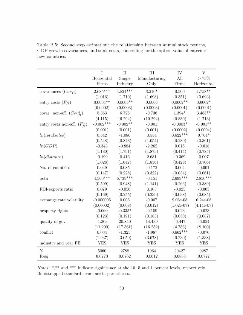
Table B.5: Second step estimation: the relationship between annual stock returns,GDP growth covariances, and sunk costs, controlling for the option value of enteringnew countries.

I II III IV VHorizontal Single Manufacturing All > 75%

Firms Industry Only Firms Horizontal

covariances (Covft) 2.685*** 4.824*** 3.216* 0.500 1.758**(1.016) (1.710) (1.698) (0.351) (0.693)

entry costs (Fft) 0.0004** 0.0005** 0.0003 0.0002** 0.0002*(0.0002) (0.0003) (0.0003) (0.0001) (0.0001)

covar. non-aff. (Covoft) 5.363 6.725 -0.736 1.394* 3.485**

(4.115) (6.294) (10.294) (0.830) (1.713)entry costs non-aff. (F o

ft) -0.002*** -0.002** -0.001 -0.0003* -0.001**

(0.001) (0.001) (0.001) (0.0002) (0.0004)ln(totalsales) 0.542 -1.080 0.554 0.622*** 0.704*

(0.548) (0.843) (1.054) (0.230) (0.361)ln(GDP ) -0.343 -0.884 -2.262 0.015 -0.018

(1.180) (1.791) (1.873) (0.414) (0.785)ln(distance) -0.199 0.416 2.631 -0.369 0.007

(1.028) (1.647) (1.836) (0.428) (0.706)No. of countries 0.049 0.085 -0.172 0.004 -0.001

(0.147) (0.228) (0.322) (0.034) (0.061)beta 4.560*** 6.739*** -0.151 2.699*** 2.850***

(0.599) (0.948) (1.141) (0.266) (0.389)FDI-exports ratio 0.079 -0.056 0.105 -0.025 -0.003

(0.169) (0.255) (0.239) (0.038) (0.085)exchange rate volatility -0.000005 0.003 -0.007 9.03e-08 6.24e-08

(0.00002) (0.008) (0.012) (1.02e-07) (4.14e-07)property rights -0.060 -0.335* -0.109 0.023 -0.023

(0.123) (0.191) (0.183) (0.050) (0.087)quality of gov -1.303 20.840 14.439 -6.447 -6.054

(11.290) (17.561) (16.252) (4.756) (8.100)conflict 0.034 -1.325 -1.987 0.662*** -0.076

(1.937) (3.050) (3.078) (0.230) (1.338)industry and year FE YES YES YES YES YES

N 5060 2788 1964 20427 9287R-sq 0.0773 0.0762 0.0612 0.0888 0.0777

Notes: *,** and *** indicate significance at the 10, 5 and 1 percent levels, respectively.

Bootstrapped standard errors are in parentheses.

50

Table B.6: Summary statistics by affiliate presence: Robustness to different mea-sures of entry costs.

Entry cost Entry cost(No. of days) (No. of procedures)

ALL FIRMS

Countries with affiliates 15.181 5.319Countries without affiliates 22.287 7.478

HORIZONTAL FIRMS

Countries with affiliates 12.054 4.314Countries without affiliates 21.567 7.318

51

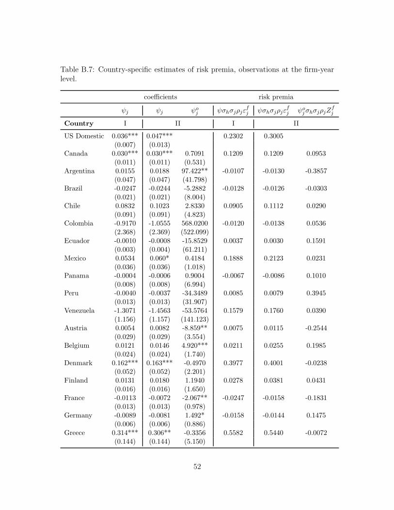
Table B.7: Country-specific estimates of risk premia, observations at the firm-yearlevel.

coefficients risk premia

ψj ψj ψoj ψσhσjρjε

fj ψσhσjρjε

fj ψo

jσhσjρjZfj

Country I II I II

US Domestic 0.036*** 0.047*** 0.2302 0.3005(0.007) (0.013)

Canada 0.030*** 0.030*** 0.7091 0.1209 0.1209 0.0953(0.011) (0.011) (0.531)

Argentina 0.0155 0.0188 97.422** -0.0107 -0.0130 -0.3857(0.047) (0.047) (41.798)

Brazil -0.0247 -0.0244 -5.2882 -0.0128 -0.0126 -0.0303(0.021) (0.021) (8.004)

Chile 0.0832 0.1023 2.8330 0.0905 0.1112 0.0290(0.091) (0.091) (4.823)

Colombia -0.9170 -1.0555 568.0200 -0.0120 -0.0138 0.0536(2.368) (2.369) (522.099)

Ecuador -0.0010 -0.0008 -15.8529 0.0037 0.0030 0.1591(0.003) (0.004) (61.211)

Mexico 0.0534 0.060* 0.4184 0.1888 0.2123 0.0231(0.036) (0.036) (1.018)

Panama -0.0004 -0.0006 0.9004 -0.0067 -0.0086 0.1010(0.008) (0.008) (6.994)

Peru -0.0040 -0.0037 -34.3489 0.0085 0.0079 0.3945(0.013) (0.013) (31.907)

Venezuela -1.3071 -1.4563 -53.5764 0.1579 0.1760 0.0390(1.156) (1.157) (141.123)

Austria 0.0054 0.0082 -8.859** 0.0075 0.0115 -0.2544(0.029) (0.029) (3.554)

Belgium 0.0121 0.0146 4.920*** 0.0211 0.0255 0.1985(0.024) (0.024) (1.740)

Denmark 0.162*** 0.163*** -0.4970 0.3977 0.4001 -0.0238(0.052) (0.052) (2.201)

Finland 0.0131 0.0180 1.1940 0.0278 0.0381 0.0431(0.016) (0.016) (1.650)

France -0.0113 -0.0072 -2.067** -0.0247 -0.0158 -0.1831(0.013) (0.013) (0.978)

Germany -0.0089 -0.0081 1.492* -0.0158 -0.0144 0.1475(0.006) (0.006) (0.886)

Greece 0.314*** 0.306** -0.3356 0.5582 0.5440 -0.0072(0.144) (0.144) (5.150)

52

coefficients risk premia

ψj ψj ψoj ψσhσjρjε

fj ψσhσjρjε

fj ψo

jσhσjρjZfj

Country I II I II

Ireland 0.0015 0.004* -1.455* 0.0207 0.0555 -0.3290(0.002) (0.002) (0.803)

Italy 0.0350 0.0382 -0.6600 0.0949 0.1036 -0.0562(0.026) (0.026) (1.032)

Luxembourg 0.0067 0.0073 0.0982 0.1067(0.008) (0.008)

Netherlands 0.028** 0.025** 0.2572 0.1355 0.1210 0.0293(0.011) (0.011) (1.018)

Norway -0.0885 -0.1016 -6.3979 -0.1347 -0.1548 -0.1606(0.108) (0.109) (4.861)

Portugal -0.0102 -0.0111 8.331** 0.0028 0.0031 -0.0340(0.022) (0.022) (4.102)

Spain -0.0037 -0.0047 0.6094 0.0009 0.0011 -0.0035(0.009) (0.009) (1.357)

Sweden 0.0009 -0.0026 0.6108 0.0042 -0.0126 0.0511(0.024) (0.024) (1.521)

Switzerland 0.0247 0.0067 -1.7172 0.0383 0.0104 -0.0569(0.039) (0.040) (2.554)

Turkey 0.0532 0.0714 16.969*** 0.0484 0.0650 0.1842(0.109) (0.109) (3.874)

United Kingdom 0.0046 0.0043 1.4119 0.0253 0.0236 0.3366(0.008) (0.008) (0.428)

Russia -0.0101 -0.0093 -29.436*** 0.0169 0.0155 0.4779(0.025) (0.025) (7.294)

Hungary 0.0244 0.0199 -3.483** 0.2094 0.1706 -0.3299(0.017) (0.017) (1.733)

Poland -0.0683 -0.0688 8.760*** -0.3709 -0.3735 0.5473(0.057) (0.057) (2.574)

Czech Republic -0.0162 0.0002 -1.5008 -0.0231 0.0003 -0.0245(0.053) (0.054) (2.488)

South Africa -0.0401 -0.0117 11.7530 -0.0473 -0.0138 0.0660(0.092) (0.092) (10.307)

Israel -0.572** -0.524** -32.222*** -0.6913 -0.6333 -0.2115(0.222) (0.223) (10.394)

Australia 0.089* 0.080* -3.1719 0.1438 0.1293 -0.0580(0.050) (0.050) (3.188)

Hong Kong 0.0203 0.0161 0.1330 0.1056 0.0000(0.016) (0.016)

India 0.2466 0.2255 1.2679 0.4075 0.3726 0.0229(0.177) (0.178) (6.535)

53

coefficients risk premia

ψj ψj ψoj ψσhσjρjε

fj ψσhσjρjε

fj ψo

jσhσjρjZfj

Country I II I II

Indonesia 0.075* 0.0655 14.1327 -0.0731 -0.0639 -0.0504(0.046) (0.047) (13.861)

Japan 0.011** 0.011** -0.1613 0.0110 0.0110 -0.0053(0.006) (0.006) (0.672)

Malaysia 0.244*** 0.228*** -0.9948 0.5780 0.5401 -0.0177(0.086) (0.087) (5.368)

New Zealand 0.0643 0.0727 -6.0231 0.1065 0.1204 -0.0826(0.088) (0.088) (6.658)

Philippines -0.0330 -0.0176 34.405*** -0.0233 -0.0124 0.1690(0.079) (0.079) (10.728)

Singapore 0.070*** 0.062*** -1.1673 0.4580 0.4057 -0.0785(0.018) (0.019) (1.570)

Korea 0.1012 0.0964 7.513* 0.1706 0.1626 0.1562(0.095) (0.096) (4.482)

Thailand -0.0351 -0.0268 -18.062** -0.0691 -0.0528 -0.2970(0.029) (0.029) (7.926)

China 0.5649 0.5217 1.0715 0.2427 0.2242 0.0069(0.578) (0.584) (8.350)

R-Sq 0.175 0.179

Notes: Bootstrapped standard errors are in parentheses. *,** and *** indicatesignificance at the 10, 5 and 1 percent levels. Both specifications include industryand year fixed effects and have n=25536.

54