Diversification and its Discontents:Idiosyncratic and Entrepreneurial Risk in the Quest for

Social Status.∗

Nikolai Roussanov†

The Wharton School, University of Pennsylvania

June 9, 2008

Abstract

Incorporating preference for social status into a simple model of portfolio choicehelps to explain a range of qualitative and quantitative stylized facts about the het-erogeneity in asset holdings among U.S. households. I specify preferences for statusparsimoniously as a function of a household’s wealth relative to aggregate wealth. Inthe model, investors hold concentrated portfolios, suggesting, in particular, a possibleexplanation for the apparently small premium for undiversified entrepreneurial risk.Consistent with empirical evidence, the wealthier households own a disproportionateshare of risky assets, particularly private equity, and experience more volatile con-sumption growth. The model is calibrated to match the empirical level of risky assetholdings without generating excessive volatility of consumption growth and cross-sectional wealth mobility.

∗I am grateful to John Cochrane, John Heaton, Tobias Moskowitz, and Pietro Veronesi for their adviceand guidance. I also benefitted from comments and suggestions by Andrew Abel, Fernando Alvarez, George-Marios Angeletos, Nicholas Barberis, Gary Becker, Frederico Belo, Hui Chen, Raj Chetty, Harold Cole,George Constantinides, Douglas Diamond, Darrell Duffie, Raife Giovinazzo, William Goetzmann, JoaoGomes, Luigi Guiso, Lars Hansen, Erik Hurst, Urban Jermann, Kenneth Judd, Ron Kaniel, Leonid Kogan,David Laibson, Marlena Lee, Hanno Lustig, Gregor Matvos, Kevin Murphy, Stavros Panageas, LubosPastor, Monika Piazzesi, ÃLukasz Pomorski, Andrew Postlewaite, Jose-Victor Rios-Rull, Jesse Shapiro,Andrei Shleifer, Harald Uhlig, Annette Vissing-Jørgensen, Jessica Wachter, Amir Yaron, Moto Yogo andStephen Zeldes, as well as seminar participants at the University of Chicago GSB, Yale, Toronto, Harvard,NYU, MIT, Stanford, BC, Columbia, Wharton, Duke, Berkeley, UCLA, Dartmouth, Lehman Brothers,and the New Economic School. This research was partially supported by the Ewing Marion KauffmanFoundation and by the National Center for Supercomputing Applications, as well as the Sanford GrossmanFellowship in honor of Arnold Zellner.

†Contact: nroussan@wharton.upenn.edu

1

1 Introduction

Diversification and risk-sharing are fundamental principles of modern finance and macroe-

conomics. However, empirical evidence suggests that household portfolios are poorly diver-

sified, with many people reporting substantial holdings of a single stock.1 For the wealth-

iest households large shares in closely held businesses constitute a particularly important

source of risk.2 Surprisingly, from a standpoint of portfolio theory, entrepreneurship does

not appear to be well compensated, implying that many investors are willing to take poorly

rewarded risks despite the availability of superior investment opportunities such as public

equity that earns a large risk premium.3

In the present paper I interpret these facts by appealing to the human desire for social

status as a key driver of risk-taking behavior. If the satisfaction brought by “getting

ahead of the Joneses” outweighs the danger of falling behind, risky activities with highly

idiosyncratic payoffs, such as entrepreneurship, can be particularly attractive. Friedman

and Savage (1948) suggest that as people move to a higher “social class” their marginal

utility of wealth rises. Consequently, they “take great risks to distinguish themselves” (p.

299), potentially exhibiting risk-loving behavior. Cole, Mailath, and Postlewaite (2001) as

well as DeMarzo, Kaniel, and Kremer (2004) show that relative wealth concerns create a

wedge in people’s attitudes towards aggregate risk and towards idiosyncratic risk, leading to

under-diversified investment portfolios. Building on these insights, I incorporate preference

for social status into a simple portfolio choice framework in which heterogeneous households

1See Curcuru, Heaton, Lucas, and Moore (2004) for a survey of the evidence on household portfoliochoice. Some of the earliest evidence of poorly diversified household portfolios was documented by Blumeand Friend (1975). Most recently, Calvet, Campbell, and Sodini (2007) measure the extent of underdiver-sification using data on portfolio composition of Swedish households.

2Heaton and Lucas (2000a) emphasize the importance of entrepreneurial risk for the households thatown much of the financial wealth in the economy. Entrepreneurial risk might not be fully diversified dueto a trade-off between risk-sharing and incentives: e.g. Bitler, Moskowitz, and Vissing-Jørgensen (2005)find evidence of agency costs affecting entrepreneurs’ holdings of business equity.

3Moskowitz and Vissing-Jørgensen (2002) find that returns on undiversified entrepreneurial investmentare no higher than the average return on publicly traded equity despite the greater risk. They refer tothis phenomenon as the “private equity premium puzzle.” Hamilton (2000) reaches similar conclusions byanalyzing the earnings differentials between self-employment and paid employment. Hall and Woodward(2007) calculate that risk-adjusted returns to venture capital-backed entrepreneurs (but not their investors)are small.

2

can optimally choose their level of exposure to idiosyncratic risk. The main prediction of my

model is that some investors optimally do not diversify: they hold portfolios concentrated

in idiosyncratic assets that earn a positive average return, such as private equity.

I model social status as an increasing function of individuals’ wealth relative to the

average wealth level, in the spirit of Duesenberry (1949).4 The key feature of status pref-

erences in my model is that wealthier households care more about their social position

in relation to consumption than do poorer ones. Adam Smith suggested that at higher

levels of income people value the “social esteem” brought on by their wealth more than the

consumption of goods and services that this higher wealth can buy (see Smith (1759), p.

70). Despite its intuitive appeal, this form of social status concerns has received relatively

little attention in the literature.5 This property implies that investors’ marginal utility

of wealth rises when they “get ahead of the Joneses” (i.e. advance their relative wealth

position). Consequently, they value a marginal dollar of wealth more highly in bad states

of the aggregate economy than in good states, even if their own wealth stays constant.

The sensitivity of marginal utility to economy-wide shocks increases aversion to aggregate

risk and leads investors to reduce their portfolios’ exposure to the public equity market.

Conversely, at any level of risk aversion status-conscious investors load more heavily on

individual-specific (e.g. entrepreneurial) risk, compared to a non-status seeking investor.

The social status model generates striking predictions for the cross-section of house-

holds’ asset holdings. Qualitatively, the richer households have a larger fraction of their

wealth invested in individual-specific idiosyncratic assets, such as private equity, as well

as risky assets generally. The standard deviations of individual portfolio returns as well

as consumption growth rates are larger for the households in the the upper half of the

distribution. The reason for this heterogeneity is that status has luxury good properties in

my model. At higher wealth levels the sensitivity to the relative position, and therefore the

4There is a growing literature documenting the importance of relative wealth or relative income concernson self-reported well-being - e.g. see Luttmer (2005).

5Important exceptions are Robson (1992) and Becker, Murphy, and Werning (2005), whose models ofstatus based on rank feature a similar property. Empirically, the intuition that the importance of statusconcerns rises with wealth is consistent with the evidence from subjective well-being surveys documentedby McBride (2001) and Dynan and Ravina (2007).

3

aversion to aggregate risk, increases, while overall risk aversion declines. Quantitatively,

the model is calibrated to match both the overall levels of risk-taking and the shares of

household wealth concentrated in a single risky asset that are observed in the U.S. data.

In particular, I match both the low shares of risky assets held by the low wealth house-

holds, and the large, highly concentrated equity shares of the very wealthy. The large

idiosyncratic component of portfolio return risk is what allows the high levels of risky

asset holdings (among the richer households) to be consistent with a smooth aggregated

consumption growth process.

As both a test and an application of the model, I evaluate its ability to match the

empirical dynamics of household wealth. Undiversified idiosyncratic risk manifests itself

in the dramatic variation of household wealth both across the population and over time.

Empirically, the cross-sectional distribution of asset holdings in the U.S. is extremely con-

centrated, yet at the same time, there is substantial mobility across wealth percentiles over

time (e.g. Hurst, Stafford, and Luoh (1998)). My model is able to account for much of

the variability in wealth holdings at the top of the wealth distribution, since the richer

households bear most of the idiosyncratic risk that drives wealth dispersion. In the sim-

ulated model a third of households in the top one percent of the wealth distribution are

displaced over the course of ten years, consistently with the data. I conclude that the

dramatic idiosyncratic risk exposure predicted by the model for the wealthiest households

is empirically reasonable.

1.1 Social status, portfolio choice, and wealth mobility: related

literature

Preferences featuring social externalities have already been applied to understanding the

lack of diversification of household portfolios.6 Much of this literature emphasizes “herding”

6Other attempts at explaining the apparent lack of diversification include models based on non-expectedutility preferences, such as cumulative prospect theory (Barberis and Huang (2005)) and rank-dependentutility (Polkovnichenko (2004)), as well as on model misspecification and learning costs (Uppal and Wang(2002), Van Nieuwerburgh and Veldkamp (2005)). Huberman (2001) and Massa and Simonov (2004) pro-vide evidence of undiversification which, they argue, is consistent with explanations based on “familiarity”.

4

and “conformism” effects of interpersonal preferences (e.g. DeMarzo, Kaniel, and Kremer

(2004) and Gollier (2004)). Shore and White (2002) argue that the external habit formation

model is able to explain the apparent tendency of investors to prefer assets local to their

community and to avoid foreign assets (the so called “home bias puzzle”). DeMarzo,

Kaniel, and Kremer (2004) show that preference for a “local good” can give rise to relative

wealth concerns, leading to undiversified portfolios, with households in each community

tilting their portfolios toward community-specific assets. Similarly, DeMarzo, Kaniel, and

Kremer (2007) demonstrate that such relative wealth concerns can lead to overinvestment

in certain risky assets. In these models investors attempt to “keep up with the Joneses”

and therefore herd by (over)investing in correlated assets. Thus, these models are not able

to explain large holdings of purely idiosyncratic assets, which is likely to be an important

component of the “private equity premium puzzle,” which is the main focus of this paper.

The prediction that allocation to risky assets is increasing in wealth appears consistent

with more standard models that feature decreasing relative risk aversion, e.g. due to non-

homothetic utility functions. Motivated by models of this class Saks and Shore (2003) find

that college students from wealthier families choose riskier careers, while Yogo (2005) exam-

ines the household consumption data from the CEX and finds that richer households have

higher consumption volatility than the poorer ones. Wachter and Yogo (2007) rationalize

the upward sloping portfolio shares of risky assets within a model with luxury goods con-

sumption. The model in this paper is particularly closely related to that of Carroll (2002),

who appeals to a “capitalist spirit” motive for wealth accumulation as a driver of decreas-

ing relative risk aversion. Even with decreasing risk aversion, standard portfolio-theoretic

models typically predict that household financial portfolios are well diversified, making it

difficult to match both the level and the concentration of risky asset holdings. The distin-

Some forms of undiversification are consistent with anticipatory utility and optimism - see Brunnermeierand Parker (2005) and Puri and Robinson (2005). Overconfidence is also cited in explaining entrepreneurialbehavior (e.g. Bernardo and Welch (2001)). Among the proposed rational explanations of low average pay-offs to entrepreneurship are real options-based models, such as Polkovnichenko (2003) and Miao and Wang(2006). While the illiquidity of private business investments might deepen the private equity premiumpuzzle (e.g. see Kahl, Liu, and Longstaff (2002)), it can also provide a potentially attractive commitmentmechanism for agents with time-inconsistent preferences (e.g. Laibson (1997)).

5

guishing feature of the relative wealth model is that it is able to capture heterogeneity in

risk taking and under-diversification simultaneously.

The analysis of social mobility from the portfolio choice perspective connects this paper

to the large literature on wealth inequality. Investment gains are potentially an important

source of wealth dispersion, especially among the rich households (Quadrini and Rios-Rull

(1997)). Most macroeconomic models of the wealth distribution have difficulty produc-

ing empirically accurate magnitudes of wealth mobility, as well as as the concentration

of wealth at the top of the wealth distribution (e.g. see discussion in Castaneda, Diaz-

Gimenez, and Rios-Rull (2003)). Following Aiyagari (1994) and Huggett (1993), standard

models consider uninsurable labor income risk as the main driver of cross-sectional wealth

dispersion. In fact, in the data consumers appear to be insured relatively well against many

exogenous idiosyncratic income shocks, such as a temporary job loss or sickness (Cochrane

(1991)). At the same time, however, there is substantial cross-sectional dispersion in wealth

accumulated over the life-cycle among households with similar earnings histories, even af-

ter controlling for various life-time shocks and heterogeneity in asset allocations (Venti

and Wise (1998)). This unexplained heterogeneity in wealth suggests a potential role for

idiosyncratic risk exposure of individual portfolios (Campbell (2006)). Quadrini (1999),

Cagetti and De Nardi (2006) and Reiter (2004) emphasize the role of entrepreneurs’ risk

exposure and capital accumulation in driving wealth concentration and social mobility.

2 An economy with relative wealth concerns

2.1 Preferences over consumption and social status

I consider a continuum of households, indexed by i ∈ Ω ⊂ R, with the total mass of 1 under

the associated measure µ.7 The wealth of household i at the beginning of time period t is

7Therefore aggregate wealth equals per capita wealth. In a discrete approximation per capita wealth isdefined as Wt = 1

N ΣNi=1W

it for some large N .

6

denoted by W it , and the cumulative distribution of normalized wealth Ft is given by

Ft (x) = µ

(i :

W it

Wt

6 x

), where Wt =

∫

Ω

W it dµ(i). (2.1)

Each household/investor has a finite lifetime of T periods in which consumption and port-

folio decisions are made, and a terminal period in which the remaining wealth (and status

conferred by it) is bequeathed to an heir born in the beginning of the period. Therefore,

there are T overlapping generations, with each new generation’s wealth being drawn from

the distribution of bequests. Households’ preferences are separable in consumption and so-

cial status, which is defined following Bakshi and Chen (1996) as household wealth scaled

by the per capita wealth.8 Specifically, at time t each investor i aged Ait year maximizes

Et

τ∑

s=t

δs−t

[(Ci

s)1−γ

1− γ+ ηW 1−γ

s

(W i

s

Ws

)]+ δτ+1ψB

(W i

τ+1, Wτ+1

)

, (2.2)

where τ = t+(T−Ait). The first term in the period utility is the standard power utility over

consumption C; the second term is the utility derived from social status.9 The parameter

that controls the relative importance of consumption and status is η > 0. It is multiplied

by an average wealth term, W 1−γt , in order to ensure that the relative importance of status

and consumption in individual utility is invariant to changes in aggregate wealth over time.

The parameter that controls the importance of bequest is ψ ≥ 0. The bequest utility is

specified as a function over terminal wealth B that has the same functional form as the

period utility over consumption, including both the absolute and the relative components:

B(W i

τ+1, Wτ+1

)=

(W i

τ+1

)1−γ

1− γ+ ηW 1−γ

τ+1

(W i

τ+1

Wτ+1

)(2.3)

8In much of the economic literature on status it is often modeled more generally as a household’s position(percentile rank) in the cross-sectional distribution of wealth (e.g. Cole, Mailath, and Postlewaite (1992),Robson (1992)). I choose the simpler specification for convenience and parsimony. The use of a separableutility specification for consumption and status is also primarily motivated by its simplicity, and is in linewith much of the literature on social status (although in contrast to Bakshi and Chen (1996))

9In the case γ = 1 I assume that the consumption utility is logarithmic.

7

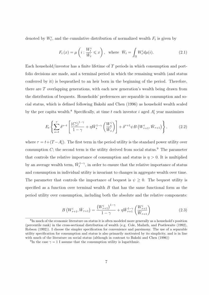
This specification implies that the bequest motive is of a “warm glow” rather than

dynastic nature. The person leaving a bequest cares about its absolute and relative size

and not directly about his heirs’ utility. This interpretation is consistent with the notion

of status-driven wealth accumulation, as it can rationalize bequests to charities and large

estates left by people with no heirs (see discussion in Carroll (2000)). At the same time,

such a specification of bequest utility could be given an altruistic interpretation in a model

where relative wealth concerns are endogenous and the utility of future generations depends

directly on their relative wealth position, as in Cole, Mailath, and Postlewaite (1992).

2.2 Technology and market structure: aggregate vs. idiosyn-

cratic risk

I model aggregate and idiosyncratic risk exposures via different assets available to investors,

following Heaton and Lucas (2004) who consider entrepreneurs’ portfolio choice and capital

structure decisions jointly. This is in contrast to much of the existing literature. Portfolio

choice models with agent-specific idiosyncratic risk commonly assume that its “amount”

is exogenously fixed, usually in the form of a stream of labor income. Conversely, models

of entrepreneurial choice (e.g. Cagetti and DeNardi (2000)) usually abstract from the

composition of financial portfolios.

A wide variety of investment opportunities provide a choice between aggregate and

idiosyncratic risk, which poses a modeling challenge. I limit the set of assets available to

the households for the sake of tractability. In the model, every household can invest in three

linear technologies with returns given by vector Ri = [Rf , Ra, Ri] distributed according to

probability density ϕ. These investment opportunities are:

• riskless storage technology with return Rf

• common risky technology (“public equity”) with return Ra

• idiosyncratic risky technology (“private equity”) with return Ri, which is individual-

specific.

8

The specification of the investment opportunities considered here captures the idea

that investors might be able to choose the combination of aggregate and idiosyncratic risk

optimally. This type of investment decision is meant to encompass human capital (career

choice) as well as entrepreneurial investment. In particular, I allow the return on the

individual-specific investment to contain an idiosyncratic component that earns a non-zero

average return:

Ri −Rf = αi + βi(Ra −Rf ) + εi,

where E[εRi|Ra] = 0. With some abuse of terminology, I label this technology “private

equity”. Market incompleteness (i.e., agents cannot invest in each others’ private asset)

is important in that it allows idiosyncratic risk to be compensated by positive expected

returns (αi > 0) without creating arbitrage opportunities.

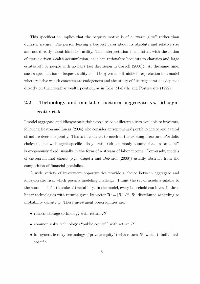
2.3 Getting ahead of the Joneses and optimal (un)diversification

Consider a one-period version of the model, in which investors maximize expected utility

over end-of period wealth and status Et

[U

(W i, W

)], where

U(W i, W

)=

(W i)1−γ

1− γ+ ηW 1−γ

(W i

W

)(2.4)

Under this specification marginal utility of wealth is positive, while the first derivative with

respect to aggregate reference wealth is negative:

UW = W−γ + ηW−γ > 0 and UW = −γηW−γ

(W i

W

)< 0 since γ, η > 0.

This is intuitive since, holding individual wealth fixed, an increase in per capita wealth

reduces the individual’s relative status and utility (such effects are often referred to in the

literature as exhibiting “jealousy” - e.g. Dupor and Liu (2003)). The individual’s risk

preferences are controlled by the partial derivatives of the marginal utility of wealth with

respect to the state variables, own wealth and per capita wealth in the economy. The

9

former, denoted by UWW , represents aversion to all wealth gambles. The latter, UWW

captures the attitude towards gambles that are correlated with aggregate wealth. When

UWW < 0 the consumer is risk averse and when UWW > 0 risk seeking. Similarly, when

UWW < 0 the consumer dislikes aggregate risk (in addition to its contribution to overall

wealth risk), and conversely when UWW > 0 the consumer seeks additional exposure to

aggregate risk, relative to a no-status benchmark.

The property that marginal value of wealth is decreasing in aggregate wealth (UWW < 0)

that represents the desire to “get ahead of the Joneses” captures the idea that an increase

in aggregate wealth, holding individual wealth fixed, lowers marginal utility of wealth. This

is in contrast to a “keeping up with the Joneses” feature (UWW > 0) that raises marginal

utility when the aggregate reference level is high.10 The intuition for “getting ahead of

the Joneses” is that higher relative status raises marginal utility of wealth (Friedman and

Savage (1948), Becker, Murphy, and Werning (2005)). Since status is an increasing function

of the ratio of own wealth to reference wealth, as defined in (2.1), a decrease in aggregate

wealth raises some people’s status, making them better off, but also raising their marginal

utility of wealth. The latter effect causes them to avoid assets that pay off poorly in such

states.

The following example captures the main qualitative feature of the relative status pref-

erences: the different attitudes towards idiosyncratic and aggregate risk and, in particular,

the “getting ahead of the Joneses” property. Consider the case with logarithmic utility of

consumption (γ = 1). Agent i’s optimization problem is

max E

[log

(W i

)+ η

W i

W

].

10The taxonomy of Dupor and Liu (2003), which is defined explicitly with respect to consumption ratherthan wealth externalities, is applicable here, since theirs is a one-period model where consumption andwealth are essentially the same. In much of the literature that features keeping up with the Joneses, theexternality is assumed to be over consumption (e.g. Abel (1990), Gali (1994), Ljungqvist and Uhlig (2000)).

10

Then standard first-order conditions yield an Euler equation for asset returns:

E

[(Ra −Ri

) (1

W i+

η

W

)]= 0.

In order to simplify exposition I assume in this example that i) the individual-specific asset

return is independent of the public stock market return, so that aggregation over households

diversifies away all idiosyncratic risk cov(Ri, W

)= 0, ii) expected returns on both assets

are the same, i.e. E [Ra −Ri] = 0. Then we have

ηcov

(Ra,

1

W

)+ cov

(Ra,

1

W i

)− cov

(Ri,

1

W i

)= 0.

If the common asset Ra is in positive net supply, it is positively correlated with aggregate

wealth (in fact, W is a linear function of Ra). Thus cov(Ra, 1

W

)is negative and, therefore,

cov

(Ra,

1

W i

)> cov

(Ri,

1

W i

), (2.5)

implying that

cov(Ra,W i

)< cov

(Ri,W i

).

This means that a “status-conscious” investor is optimally exposed to more idiosyncratic

risk and less exposed to aggregate risk than a neoclassical investor. In particular, if Ra

and Ri are identically distributed, standard preferences (η = 0) imply that cov (Ra,W i) =

cov (Ri,W i) and therefore the weights on two assets are equal. Under status preferences

that is no longer the case: since the optimally chosen individual wealth process covaries less

with the aggregate return than with the idiosyncratic return, this implies that the weight

on the former asset in the household’s portfolio is lower than on the latter. As follows

from (2.5), the magnitude of the difference in portfolio shares depends on the strength of

preference for social status, controlled by parameter η, as well as the covariance between

aggregate risk and per capita wealth.

11

3 Quantitative analysis

In this section I define the individual households’ decision problem as well as the equilibrium

concept associated with the dynamic version of the model, and describe the computational

strategy employed in solving for an approximate equilibrium numerically.

3.1 Dynamic optimization

Each household i aged Ait at time t solves the following recursive problem:

V (W it , Wt, A

it; It) = max

C,a

(Ci

t)1−γ

1− γ+ ηW 1−γ

t

W it

Wt

+ δE[V (W i

t+1, Wt+1, Ait+1; It+1)

∣∣ It

]

,

(3.1)

subject to the resource constraint

W it+1 =

(W i

t − C it

)a

i′t R

it+1,

where the vector of portfolio allocations to the three assets is given by ait = [1− ai

t − ait, a

it, a

it].

The agents cannot influence their current-period status, which is determined by their

beginning-of-period wealth endowment. Consequently, standard dynamic programming

arguments can be applied to analyzing the problem quantitatively.

It is convenient to restate the problem in a way that exploits scale-independence. Let

cit =

Cit

W it

, sit =

W it

Wt

, Gt+1 =Wt+1

Wt

. (3.2)

Then the value function (3.1) above can be written as

V(W i

t , Wt, Ait; It

)=

[v(si

t, Ait; It) + ηsi

t

]W 1−γ

t , (3.3)

where the scale-invariant function v(sit, A

it; It) solves the corresponding recursive problem

12

(see appendix A).

3.2 Equilibrium

Since aggregate (per capita) wealth is a state variable that enters the objective function of

households, optimal consumption and investment policies that are solutions to the dynamic

programming problem (3.1) generally depend on the wealth distribution F and its evolution

over time via the implied law of motion for aggregate wealth growth G. Specifically, we

can write

Gt+1 =Wt+1

Wt

= E[si

t

(1− ci

t

) (1− ai

t − ait

) |It

]Rf

+ E[si

t

(1− ci

t

)ai

t

(αi + εi

t+1

) |It

]

+ E[si

t

(1− ci

t

) (ai

t + aitβ

i) |It

]Ra

t+1,

(3.4)

where the expectations are taken with respect to the cross-sectional distribution µ as well

as idiosyncratic return realizations, and the time-t information set It includes the mapping

between individual households and their wealth levels summarized by Ft. This law of

motion is exogenous to any individual household. At the same time, the fact that per

capita wealth in the next period, Wt+1, depends on the previous period average wealth

Wt as well as on the consumption and investment choices made by households at time t,

imposes additional restrictions on the solution procedure. These restrictions lead to the

following notion of equilibrium.

Definition 1. A status/investment equilibrium consists of

• household value functions V and optimal policies [C, a]

• law of motion for the growth rate of aggregate wealth Gt+1 as a function of aggregate

return Rat+1, household wealth levels contained in It, and households’ optimal policies

The equilibrium is a fixed point of the mapping between the aggregate wealth process

that is taken as exogenous by investors and the endogenous evolution of aggregate wealth

13

resulting from individual optimization.

3.3 Numerical solution

The equilibrium notion introduced above implies that the state space, which includes the

space of wealth distributions, is potentially infinite-dimensional. Finding such an equi-

librium in practice is infeasible. Instead I approximate the dynamics of the endogenous

aggregate state variable, similarly to Krussell and Smith (1998).

Note that the law of motion for aggregate wealth (3.4) can be written as

Gt+1 = ξ0 (It) + ξ1 (It) Rat+1,

where ξ0 (It) and ξ1 (It) are determined in equilibrium and can vary over time with the

wealth distribution. In my numerical solution I approximate them with constants by simu-

lating the model forward and projecting the resulting path of aggregate wealth growth on

the return realizations. I verify that the resulting law of motion is indeed (approximately)

time-invariant. To check that the evolving wealth distribution does not alter the law of

motion I condition the projection on lagged values of G and confirm that this does not

improve the forecasting power of the linear projection.

The numerical approximation procedure therefore consists of solving the individual

optimization problems, simulating future wealth distributions for a large number of periods

using the optimal policies, updating the resulting law of motion for aggregate wealth,

and repeating the procedure until the law of motion stabilizes. Further details of the

computational procedure are provided in appendix B.

3.4 Parametrization

I solve the model for T = 7 periods so that each period corresponds to a 10-year in-

vestment horizon. Thus, if the youngest agents enter the model at age 20 then the last

decision-making period corresponds to the age of 80 years. Table I lists the parameters of

14

the investment opportunity set as well as the benchmark values of preference parameters.

The unconditional means of the stock return and the risk-free rate (i.e., 10-year Treasury

bond yield) approximately match those in the U.S. data, at annualized values (for cor-

responding logarithmic returns) of 11 and 5 percent, respectively11. The risk-free rate is

constant. The equity returns are i.i.d. I assume that the expected excess return on the

idiosyncratic asset is equal to the public equity premium, consistent with the findings of

Moskowitz and Vissing-Jørgensen (2002). I assume that the standard deviation of the id-

iosyncratic project/private equity return is three times as high as that of the public equity,

which is similar to the volatility of publicly traded individual stocks (see Campbell, Lettau,

Malkiel, and Xu (2001)). This implies annualized standard deviations of public and pri-

vate equity logarithmic returns of 15 and 45 percent, respectively. Heaton and Lucas (2004)

and Polkovnichenko (2003) consider similar volatility levels in calibrating entrepreneurial

project hurdle rates.

I assume a discrete two-state distribution for the public equity return, with a high

realization being twice as likely as the low realization, which implies values of Ra =

[1.028910, 1.148310]. I let idiosyncratic states follow a lognormal distribution and use Gauss-

Hermite quadrature (with 10 nodes along the idiosyncratic dimension) to evaluate expec-

tations.12 In the benchmark calibration I allow private equity returns to covary positively

with public equity by setting βi = 0.5. This is qualitatively consistent with the empirical

evidence in Heaton and Lucas (2000b) that income streams from proprietary businesses are

positively correlated with the stock market return. For the two-state public equity return

process I use this beta to restrict the conditional mean of private equity return in each of

the aggregate states.

The initial wealth distribution used as a starting point for the iterative procedure is

calibrated using the percentiles of the U.S. wealth distribution from the 2001 Survey of

11This assumption overstates the real risk-free rate in the data, however, it allows me to sidestep thetension generated by the equity premium and risk-free rate puzzles in calibrating aggregate portfolio hold-ings. Since explaining these puzzles is not the focus of this paper, I parameterize the model to make themleast pronounced.

12See Judd (1999) for a general discussion of numerical integration.

15

Consumer Finances. Table I displays the set of points used to approximate the distribution.

4 Status model vs. data

In this section I evaluate the ability of the social status model to explain quantitative as well

as qualitative features of the data. First, I calibrate the model to match the asset holdings

and consumption volatility at the aggregate level. I also calibrate the model with standard

CRRA preferences to match the same features of the data as a benchmark. I then evaluate

both models’ predictions for the cross-section of individual portfolio allocations. I show

that the social status model does a substantially better job explaining the cross section

of household asset holdings than does the standard model matched to the same aggregate

quantities. I also evaluate the model’s predictions for the individual wealth variability over

time as well as discuss its implications for savings behavior and entry into entrepreneurship.

4.1 Calibrating the model: aggregates

The empirical and simulated moments for the aggregate quantities of interest are displayed

in table II. The primary targets of my calibration are two key statistics of the data on

individual household portfolio allocations: average holdings of risky assets (specifically,

public and private equity) and the degree of portfolio concentration. While prices are

interpreted as exogenous technology parameters in the model, I set them in accordance with

empirical estimates. I then choose preference parameters - utility curvature γ and status

weight η - so as to match closely the two moments of household portfolio holdings.13 I use

data from 2001 Survey of Consumer Finances to estimate the average share of household

assets allocated to risky assets (including stocks, mutual funds, corporate bonds, private

businesses, etc.) and the average share allocated to “concentrated equity” - the household’s

largest risky asset holding (such as private business or individual stock). I only consider

households who report positive holdings of risky assets, since in my model all households

13Piazzesi and Schneider (2007) propose a framework for modeling both asset prices and quantitiesendogenously in a similar portfolio-choice context.

16

are marginal in the stock market since since there are no costs associated with stock market

participation. Appendix C describes the data in detail. The model counterparts of these

moments are the average share of wealth allocated to risky assets (both public and private

equity) and the average share of private equity.

In addition, I use the set of empirical facts about aggregate consumption growth volatil-

ity to constrain my calibration. I compare the standard deviations (annualized, in percent-

age points) of average logarithmic consumption growth generated by the model for a range

of parameter values with those from the U.S. data. The reported consumption volatility

measures are based on the estimates obtained using micro data from the Consumer Ex-

penditure Survey (CEX). The estimates of volatility of average consumption growth are

from Malloy, Moskowitz, and Vissing-Jørgensen (2005); the average consumption growth

volatility is based on the quarterly estimates of Wachter and Yogo (2007); both studies use

CEX household consumption expenditure data for nondurable goods and services. I also

report the standard deviation of growth in the logarithm of per capita consumption from

NIPA. These comparisons should be viewed with some caution, since the model numbers are

based on 10-year periods, whereas consumption data are based on quarterly consumption

growth observations (however, Malloy, Moskowitz, and Vissing-Jørgensen (2005) estimate

a growth rate of quarterly consumption over long horizons; I use the 20-quarter estimate).

Household-level consumption data are available in the CEX for less than 25 years, making

it difficult to estimate the volatility of consumption growth between 10-year periods. Still,

since aggregate consumption process is close to a random walk at the annual frequency,

this problem might not be too severe.

Alongside the empirical estimates of consumption volatility the table displays corre-

sponding quantities obtained using simulated data produced by the social status model for

the consumption curvature parameter γ = 10 and status weight η = 1 - the values chosen

to approximately match the empirical quantities. I also report the corresponding model

quantities for the case η = 0 (i.e. standard CRRA preferences with no status concerns) and

consumption curvature γ = 8, which is also chosen so as to best match the target moments.

The social status model can match the average portfolio shares fairly closely. The model

17

slightly understates the average share of risky assets (total equity in total assets), at 25

percent vs. 28 percent in the data. The model matches the degree of portfolio concentration

at the aggregate level exactly, reproducing the 18 percent of total equity concentrated in

the “single largest asset”. Consequently, the model only slightly overstates the average

fraction of total assets devoted to private equity, at 6 percent. The model can match these

asset quantities without generating counterfactually high volatility of consumption growth:

the annualized standard deviation of log average consumption growth is 1.85% in the model

versus 1.71% in the data; the volatility of average consumption growth is greater, at just

under 5 percent both in the data and the model.

The standard power utility (CRRA) model calibrated similarly to the status model can

also match the above empirical quantities fairly well. The CRRA model with curvature

γ = 8 matches the share of risky assets almost exactly, at 27 percent, but underestimates

the degree of portfolio concentration, with 15 percent of risky assets invested in private

equity (or 4 percent of total assets). The power utility model matches aggregate con-

sumption volatility almost exactly, and overestimates the volatility of average stockholder

consumption growth by a third of a percentage point. Both the status and the CRRA

model produce greater average consumption growth volatility across households, at 6.6

and 6 percent, respectively. This is due to the fact that some of the consumption volatility

is idiosyncratic, especially for the status model.

The fact that both the status model and the CRRA model can match aggregate quan-

tities that I target equally well is not surprising. The average holdings of risky assets and,

in particular, concentrated equity across the U.S. households are fairly low. Thus, the

under-diversification puzzle does not arise at the aggregate level. In order to see the puzzle

one needs to focus on households that are likely to own concentrated assets, in particular,

the wealthy.

18

4.2 Evaluating the model: cross-section

The main challenge for the portfolio choice model is to explain the heterogeneity in asset

holdings across households, given the constraint imposed by matching the aggregate quanti-

ties. The empirical measures of risk-taking and diversification that I analyze are averages of

portfolio shares taken over two subsamples of households, subdivided into wealth percentile

groups. The first subsample includes all “stockholders” defined broadly as households who

own both directly held equity and equity held through mutual funds or other managed

accounts. The second one is “stockholders with concentrated holdings” - a subset of stock-

holders that report positive holdings of one of the following: directly held individual stocks,

private business, investment real estate, and other similar risky assets. As discussed above,

my empirical analog of “private equity” in the model is the single largest asset from the

above list owned by a household. In addition, I look at total “undiversified” equity, which

is the sum of all such concentrated holdings (i.e. all equity, public and private, that is held

directly rather than in managed accounts).

In order to evaluate the model’s ability to explain portfolio allocation decisions I consider

the variation in the portfolio shares across the wealth distribution. The average allocations

by wealth quantile obtained from the SCF are summarized in table III. The salient feature

of the data is that both the share of risky assets in households’s portfolios and the degree

of asset concentration in the largest risky asset are increasing in wealth.

Table IV reports the corresponding quantities produced by the calibrated social sta-

tus as well as for the power utility model. The social status model broadly matches the

cross-sectional patterns of risky asset holdings (Panel A). The average allocation among

the bottom half of the wealth distribution is around 20 percent in the data (19 for all stock-

holders and 24 for those with concentrated equity). This is matched almost exactly by the

model, at 23 percent. Consistently with the data, the share of risky assets in the social

status model is increasing in wealth. At the top 5th percentile of the wealth distribution

households in the data invest just over half of their wealth in equities, which is captured by

the model. For the highest (top one percent) wealth percentile, the model overshoots the

19

risky asset allocation for stockholders (63 percent in the data), almost matching the aver-

age allocation among business owners/concentrated shareholders at around 80 percent. By

contrast, the standard power utility model, which features constant portfolio shares across

the wealth distribution because of homotheticity, cannot match the heterogeneity in port-

folio allocations. The equity share of 27 % predicted by the CRRA model (Panel B) are

not too far from the empirical estimates for the bottom 90 percent of the wealth distribu-

tion. However, within the top decile of the distribution, the standard model dramatically

understates the level of risky asset holdings.

Explaining the cross-section of portfolio concentration is an even greater challenge. The

social status model does a good job of matching the average portfolio shares allocated to

private equity among all stockholders, as well as its increasing profile. The model predicts

that on average 12 percent of equity, or 3 percent of total assets, is concentrated in the

idiosyncratic asset in the lower deciles of the wealth distribution. This is similar to the

average shares in the data, as well as to the predictions of the CRRA model. In the

top decile of the distribution, however, the concentration shares increase sharply, up to

almost 30 percent of total assets for the richest one percent of households. The CRRA

model cannot match this increase. The social status model exhibits a sharp increase in

concentration shares over the top wealth percentiles, predicting that the entire risky asset

holdings of the top one percent of households are comprised of private equity (in fact, their

equity stake is 6 percent short the public stock market). This prediction appears extreme

relative to the average empirical shares of the single largest concentrated equity holdings

displayed in table III. However, if we extend the notion of concentrated equity holdings

to include all “undiversified” equity, the difference becomes less dramatic. In the data, for

households in the top one percent of the wealth distribution and for those in the next 4

percent, the average shares of total equity holdings that are undiversified are 77 and 54

percent, respectively, corresponding to 51 and 31 percent of total assets. Conditional on

households having non-zero holdings of such concentrated equity assets these quantities

are even greater, with over 80 percent of equity held by top 1 percent of households in the

form of undiversified investments. These quantities are still lower than those predicted by

20

the model for the wealthiest household groups. However, it is difficult to assess the extent

to which the model overstates under-diversification of the rich using the SCF data. It is

possible that some of the equity positions that I classify as “diversified,” such as those

held in mutual funds and “managed accounts” are in fact highly exposed to idiosyncratic

risk. In particular, it is likely that some of the “managed account” holdings of the very

wealthy might include hedge fund and private equity fund investments, which can have

large idiosyncratic risk exposure.14

The ability to match the levels of risky asset holdings and portfolio concentration of the

richest households without generating excessive volatility of aggregate consumption growth

is a distinctive feature of the social status model. The standard CRRA portfolio model

with γ = 8 calibrated to match the same aggregate quantities cannot match either the

heterogeneity in risk taking or the extent of portfolio concentration among the rich. The

reason the social status model is able to reconcile the aggregate facts with the evidence

on portfolio holdings of the very wealthy is that its prediction of high levels of portfolio

concentration in a (largely) idiosyncratic asset for investors with high wealth relative to

the average.

In the model, individual consumption growth volatility is sharply increasing in wealth

along with the volatility of portfolio returns, reaching 20 percent for the top wealth groups

(table IV).15 Much of this volatility is idiosyncratic, driven by the returns on “private

equity.” The model’s allocations to private equity are empirically plausible in that they

generally follow the same increasing pattern as the allocation to undiversified equity hold-

ings in the data, although the predicted magnitudes are higher for the top wealth groups.

Note, however, that matching these statistics is hard due in part to the measurement dif-

ficulties: unlike the public stock market, households’ private equity returns are largely

unobservable. Nevertheless, the magnitudes are sufficiently similar to conclude that the

14Calvet, Campbell, and Sodini (2007) document that wealthier households appear to hold better-diversified portfolios than poorer ones, but at the same time also invest more aggressively, and as a resultare exposed to more idiosyncratic risk.

15Wachter and Yogo (2007) report estimates of individual consumption volatility growth by wealth groupsthat are of similar magnitudes.

21

model can broadly match the empirical patterns of risk taking and the degree of portfolio

concentration simultaneously.

4.3 Understanding portfolio heterogeneity

What drives the heterogeneity in portfolio allocations in the social status model? “Getting

ahead of the Joneses” property of status preferences implies a wedge between the relative

risk aversion towards any wealth gambles, and relative aversion to risk that is correlated

with the per capita wealth. Further, the effect of “getting ahead of the Joneses” increases

with relative wealth in a non-linear fashion, simultaneously driving down the risk aversion

of the wealthiest investors and thus increasing their optimal exposure to idiosyncratic risk.

In order to illustrate the intuition behind this result, it is useful to consider once again

the simplified one-period version of the model in 2.4. Since in the one period case the utility

is defined directly over wealth, we can compute the relevant measures of risk aversion. The

Arrow-Pratt coefficient of relative risk aversion of agent i is

RRA = −W iU iWW

U iW

=γ (W i)

−γ

(W i)−γ + ηW−γ=

γ

1 + η(

W it+1

Wt+1

)γ ,

which is a decreasing function of relative wealth,W i

t+1

Wt+1, and is bounded from above by γ,

its limit at zero wealth. It tends to zero as relative wealth grows.

As a way to measure the desire to “get ahead of the Joneses” we can similarly calculate

the “relative aversion to aggregate wealth risk” (RAWRA), a quantity analogous to a

Merton-type hedging demand that stems from the state-dependence of the utility function.

Define

RAWRA = −WU iWW

U iW

=γηW−γ

(W i)−γ + ηW−γ=

γη(W i

t+1

Wt+1

)−γ

+ η,

which is an increasing function of relative wealth, with the upper limit equal to γ. The

lower limit as relative wealth falls is zero. Thus, the poorest individuals, while most risk

averse, are the least averse to aggregate risk. Conversely, the wealthiest individuals are the

22

least averse to pure wealth gambles, but also the most averse to aggregate fluctuations. The

degree of divergence in risk attitudes for intermediate values of relative wealth is controlled

by the magnitude of η, the status weight. The greater this parameter is, the steeper the

decrease in risk aversion and the increase in aversion to aggregate risk as relative wealth

goes up. For η = 1 the two types of risk aversion are of equal magnitudes for the average

investor (i.e. atW i

t+1

Wt+1= 1). For η > 1 the aggregate risk aversion overtakes the RRA

coefficient at lower relative wealth levels. Figure 1 plots these two measures of risk aversion

- RRA and RAWRA - as functions of relative wealth, si = W i

Wfor the case γ = 10, η = 1.

The sum of the two measures of risk aversion in this example is constant across wealth

levels and equal to γ.

Following the state-variable hedging intuition of Merton (1973), the overall allocation of

assets to securities that bear aggregate risk is determined by a combination of overall risk

aversion and the “hedging demand” for insurance against fluctuations in per capita wealth.

In particular, risk averse individuals with “keeping up with the Joneses” preferences might

require less compensation for bearing aggregate wealth risk than for purely idiosyncratic

risk (e.g. see Gollier (2004)). Conversely, low risk aversion to pure wealth gambles can be

consistent with low allocation to aggregate assets even in the face of a high risk premium.

The latter feature of “getting ahead of the Joneses” preferences is consistent with the

view of the aggregate equity premium that emphasizes low individual risk aversion towards

idiosyncratic gambles (e.g. see discussion in Kocherlakota (1996) and Cochrane (1997)).

The intuition behind the cross-sectional differences in risk attitudes is that status pref-

erences exhibit more curvature with respect to consumption than with respect to (relative)

wealth, which implies that the latter is treated by consumers as a luxury. This drives down

the risk aversion towards pure wealth gambles at high wealth level. At the same time,

since relative wealth position is a “luxury,” it is relatively more important to the wealthy,

so that the strength of “getting ahead of the Joneses” motive increases with wealth, driv-

ing up the aversion to aggregate risk. Carroll (2002) argues that a preference for wealth

as a luxury good is key to explaining the heterogeneity in portfolio composition across

households, in particular the fact that the rich save more as a fraction of their wealth than

23

the poor and that they hold a much larger share of risky assets (including entrepreneurial

ventures) in their portfolios. However, the social status preferences analyzed here are not

simply a way of introducing decreasing relative risk aversion. A model that has the latter

feature but does not exhibit “getting ahead of the Joneses” might be able to explain the

increasing pattern of risky asset holdings, but is unlikely to match the degree of portfo-

lio concentration among the wealthy households. Applying the standard assumption that

individuals’ marginal utility does not depend on aggregate wealth directly implies that

households’ optimal portfolios are well diversified and closely resemble the aggregate stock

market index. Consequently, the resulting aggregate consumption growth should exhibit

greater variability.

4.4 Wealth mobility

Does the social status model imply too much variability in individual consumption and

wealth, in particular for the richest households? The model does predict high volatility

of portfolio returns and consumption growth for the top one percent of households, at 28

and 20 percent (log, annualized), respectively. Unfortunately, it is impossible to assess

directly whether these quantities are empirically reasonable. Data on individuals’ portfolio

returns is unavailable in the U.S., while consumption data from the CEX lacks sufficiently

long panel dimension for estimating individual consumption growth volatility over long

horizons. In addition, the CEX does not do a very good job sampling the wealthiest

households. Thus, in order to evaluate the model’s predictions for the degree of exposure

to idiosyncratic risk I look at the cross-sectional dynamics of household wealth using data

from the Panel Study of Income Dynamics (PSID). Although this dataset, like the CEX,

undersamples the rich households, it has a long enough panel dimension that allows me to

estimate changes in household wealth over 10-year periods, which match the horizon in my

simulated model.

While it is well known that the distribution of household wealth in the U.S. is extremely

wide and highly concentrated, there is also a substantial amount of cross-sectional wealth

24

mobility over time. I estimate 10-year transition probabilities of wealth deciles following

Hurst, Stafford, and Luoh (1998) They estimate transition probabilities using the PSID

wealth supplements over the period 1984-1994. I update their estimates with data from

the 1999 supplement. I adjust the estimated transition rates to limit the influence of

measurement error and, most importantly, to remove life-cycle accumulation/decumulation

effects that are absent in my model, in order to provide an appropriate benchmark for

evaluating the model’s predictions. Details of this estimation can be found in appendix C.

Table V displays the probabilities of moving upwards or downwards and staying in the

same percentile group conditional on being in a given wealth quantile at the beginning of a

ten-year period. The empirical transition matrix displays a substantial degree of mobility,

especially in the right tail of the wealth distribution (panel A). Among the households in

the top one percent two thirds are staying in the same decile, and one third falling into a

lower decile. In the 95th to 99th percentile group, over half of all households fall behind

after 10 years. At the same time, the movement between the top and the bottom half of the

distribution is very limited, with 98 percent of households in the bottom 50 percent remain

there after 10 years. As shown in the table V, within the groups of households that report

positive holdings of stocks and private businesses the estimates of transition probabilities

are very similar, with a slightly higher mobility in the middle deciles.

The social status model is able to generate patterns of social mobility that very closely

mimic those in the data for the top percentiles of the wealth distribution. The quantitative

features of the transition distribution for the status model are summarized in table V (panel

B) alongside the empirical estimates (displayed in . Note that for the top 1 percent of the

distribution the model matches the empirical transition probabilities almost exactly. In

contrast to the social status model, the standard power utility model (panel C) produces

highly persistent cross-sectional wealth distribution, with persistence probabilities of 95

percent in the top percentile of the distribution (compared to about 67% in the data and

under the status model). For lower percentile group the match between the social status

model and the data is less close, but the model still outperforms the neoclassical benchmark.

Overall, even though the social status model is not designed specifically to explain social

25

mobility, it does a good job of matching the empirical facts for the mobility in the upper

end of the wealth distribution. It is therefore likely that the model’s predictions for the

degree of households’ exposure to idiosyncratic investment risk are reasonable.

4.5 Entrepreneurship and concentration

In matching the cross-section predictions of the social status model for degree of portfolio

concentration I have so far ignored the fact that a large fraction of households, even among

stockholders, has no concentrated holdings. In the context of the model, this might not be

surprising if not all investors have access to idiosyncratic investment opportunities that earn

a positive abnormal return (“alpha”). Separating households who do own concentrated

assets helps to match the model’s predictions for the idiosyncratic risk exposure of the

wealthiest investors’ portfolios. At the same time, conditioning on participation in “private

equity” market also reveals that the model dramatically understates the degree of portfolio

concentration in the bottom half of the wealth distribution. As documented in table III

(panel B), households in the lower half of the distribution that do own idiosyncratic assets

on average have between 80 and 90 percent of their total equity concentrated in such

investments, which corresponds to 20 percent of their total assets. These concentration

shares decline somewhat at higher wealth levels before displaying the sharp increase in

the top 5 percent group. In contrast, in the model the poorer households have the lowest

concentration shares (3 percent of total assets allocated to private equity).

The reason for the discrepancy is not surprising. In the model I allow households

to invest a small fraction of their wealth in private equity. In the data, the concentrated

equity stakes, especially among the poorer households, are driven by business owners. Given

the potential importance of asymmetric information in the private equity market and in

financing of small businesses, incentive considerations should dictate that the entrepreneurs’

stakes in their businesses must be large relative to their outside assets. In fact, Bitler,

Moskowitz, and Vissing-Jørgensen (2005) show that this prediction is indeed borne out in

the data. Still, this does not explain why poorer households choose to become entrepreneurs

26

if doing so requires a potentially dramatic increase in portfolio and consumption risk relative

to other investment opportunities. For example, setting the minimum required business-

owner’s private equity stake to be 20% of total assets, which is consistent with estimates

obtained by Bitler, Moskowitz, and Vissing-Jørgensen (2005), would imply that, in the

social status model, only the wealthiest 5 percent of households find it optimal to become

entrepreneurs. In order to confirm this intuition I solve the model restricting the share of

private equity in total assets to be at least 20 percent, or else zero. Table IV (panel C)

displays the resulting cross-section of private equity shares. Indeed, they are zero for all

households outside of the top decile of the wealth distribution.

One possibility for rationalizing this result with the data is to allow for heterogeneity in

investment opportunities among investors. In particular, suppose individuals draw idiosyn-

cratic entrepreneurial projects randomly from a distribution of systematic risk exposures.

Then, for all but the very wealthy households, entry into entrepreneurship is driven by

the diversification benefit of private equity. For example, suppose some entrepreneurs have

access to projects that provide a hedge for aggregate risk in the form of a negative beta

with the public equity. Then a concentrated investment in such a project might be opti-

mal even for the poorest investors, for whom the status-seeking motive is very weak. The

bottom line of table IV (panel C) shows private equity shares simulated from the model

with the minimum concentration constraint of 20 percent and negative systematic risk of

private equity: βi = −0.5. It is evident that in this case, when private equity is a good

hedge against the risk of public equity, even the households in the bottom half of the wealth

distribution are willing to invest a fifth of their assets in it. The probability of drawing a

project with such a large diversification benefit is likely to be small empirically, however.

This is consistent with the huge discrepancy in the rate of participation in the private

equity market reported in table III between the richer and the poorer households. Only 8

percent in the bottom half of the wealth distribution own concentrated equity, compared

to 83 percent of households in the top one percent of the distribution.

An interesting direction for future research is to calibrate a model with explicit het-

erogeneity in private equity investment opportunities. One likely prediction is that the

27

nonlinear effect of “getting ahead of the Joneses” on risk preferences might lead to a sharp

increase in participation rates at the very top of the wealth distribution, with little variation

across lower percentile. Hurst and Lusardi (2004) find that wealth itself does not predict

entry into entrepreneurship, except for the top 5 percent of the distribution, and that the

liquidity constraints, while potentially important, do not explain entry rates either. At

the same time, empirically there is some evidence of a link between concentration of finan-

cial portfolios and entrepreneurship: Calvet, Campbell, and Sodini (2007) report that the

portfolios of entrepreneurs are on average less diversified than those of non-entrepreneurs.

This evidence lends further support to the unified view of household diversification offered

in this paper.

4.6 Saving and consumption dynamics

The social status model generates considerable heterogeneity in saving rates. The optimal

consumption - wealth ratios reported in table VI show that the richest 10% of the households

consume a much smaller function of their wealth than the poorest half, and consequently

save more. The youngest households at the bottom of the wealth distribution consume 45

percent of their initial wealth (over a 10-year period), as do power utility households. The

richest 10 percent of the young (e.g., 20-year olds) consume only 11 percent. The difference

is even more dramatic for the old households: the poorest 25 consume 60 percent of their

wealth in the second-to-last period of their lifetime (i.e. at age 80), while the richest 5

percent still consume about 12 percent, thus leaving a disproportionately large amount of

wealth for their heirs. This prediction of the model is consistent with the stylized empirical

observation that the rich elderly do not dissave as predicted by the standard life-cycle model

(e.g. see Dynan, Skinner, and Zeldes (2004)). The intuition for the high saving rate among

the very rich is that the future status utility provides additional benefit for saving, above

an beyond the desire to smooth consumption over time. This motive is particularly strong

for the wealthy, since future status is relatively more important to them. This prediction is

typical for models where wealth confers social status: e.g. Cole, Mailath, and Postlewaite

28

(1992) and Corneo and Jeanne (1999) discuss the “oversaving” effects generated by relative

wealth concerns.

The differences in consumption-wealth ratios across the wealth distribution are not

driven by the bequest motive as such. Rather, they are due to the fact that the marginal

utility of wealth is increasing in relative wealth (a consequence of “getting ahead of the

Joneses” property). This shifts the importance from consumption towards wealth accumu-

lation as individual’s wealth grows (relative to the average). Some of the empirical facts

concerning the heterogeneity in saving rates can be explained by other models in which

preferences for bequest are non-dynastic and have luxury-good properties (e.g. Carroll

(2000), DeNardi (2004)). The social status model possesses this desirable feature even

though it was not designed specifically to explain savings behavior.

A limitation of my model that does not allow me to match the saving rates produced

by the model to the data quantitatively (rather than qualitatively) is the absence of labor

income. I leave out labor income from my model in order to focus attention on the endoge-

nous choice of exposure to idiosyncratic risk, which is driven by relative wealth concerns. In

order to expose the model’s mechanism most clearly, I avoid encumbering it with another

source of idiosyncratic risk. The illiquidity of individual human capital and its deprecia-

tion with age can be major determinants of saving behavior as well as portfolio choice over

the life cycle (e.g. see Viceira (2001), Cocco, Gomes, and Maenhout (2005), Gomes and

Michaelides (2005) and Storesletten, Telmer, and Yaron (2007)). However, it is likely that

these effects are muted for the very wealthy, whose investment behavior is the primarily

focus of this paper, since for them human capital is likely to constitute a much smaller

fraction of total wealth than for an average U.S. household. Undoubtedly, incorporating

labor income into the social status model would be important for evaluating its predictions

for the entire cross-section of households, and is a promising venue for future research.

29

5 Discussion and Concluding Remarks

In this paper I address the limited diversification of household portfolios together with

the apparent lack of a premium for undiversified entrepreneurial risk by considering the

investment choices of individuals who exhibit a preference for social status. The assumption

that marginal utility of wealth increases with relative status leads investors to optimally

hold undiversified portfolios in equilibrium. This feature of the model suggests that at

least some of the empirically observed cross-sectional dispersion in accumulated wealth can

be understood using a simple portfolio-based approach that allows the amounts of both

aggregate and idiosyncratic risk in the economy to be determined endogenously. Thus it

supports the argument of Friedman (1953) who emphasizes the role of individual choice

and, in particular, risk preferences in shaping the distribution of income and wealth.

The model also has potential implications for the study of investment and, consequently,

economic growth. Standard macroeconomic theory is predicated on the assumption that

the demand for diversification leads households to pool and share their idiosyncratic risks.

Perfect risk sharing is prevented, however, by the incompleteness of insurance markets

due to asymmetric information and limited enforcement of contracts. Such market im-

perfections impose costs on society in the form of foregone investment opportunities, due

to the inability of agents to share idiosyncratic risk of individual projects. Preference

for social status can mitigate this problem, since it can lead investors to take on more

undiversified idiosyncratic risk than predicted by the standard theory, unleashing greater

entrepreneurial investment and spurring economic growth. This intuition is similar to the

argument of Robson (1996) that evolutionary forces favor agents who are less averse to

idiosyncratic than to aggregate risks, since the former are “diversified” at the macro-level,

while the latter are not. I provide an example of how status-generated “overinvestment” in

individual-specific projects can be socially optimal in economies with limited risk-sharing

in Roussanov (2006). This possibility appears consistent with the evidence of Anderson

and Reeb (2003) that companies with concentrated founding-family ownership are less, not

more, diversified, than other firms, contrary to the predictions of standard theories, such

30

as Shleifer and Vishny (1986). Corneo and Jeanne (1997) and Corneo and Jeanne (2001)

make a related argument that “oversaving” generated by social status concerns can help

overcome negative externalities arising from technological spillovers, and therefore lead to

optimal economic growth.

A link between preferences with relative status concerns and economic growth could

help explain the divergent patterns of entrepreneurship and economic development across

countries. Becker, Murphy, and Werning (2005) suggest that in societies in which the

distribution of status is exogenously fixed (and thus not necessarily closely tied to relative

wealth) one should observe less risk-taking. Rules governing assignment of status in a

society can arise endogenously as evolutionary outcomes (e.g. see discussion of “wealth-is-

status” vs. “aristocratic” equilibria in Cole, Mailath, and Postlewaite (1992)). Differences

in cultural and social norms can potentially be at least as important as differences in

economic policies in explaining the variation in the pace of economic growth around the

world.

References

Abel, Andrew B., 1990, Asset prices under habit formation and catching up with the Joneses,American Economic Review 80, 38–42.

Aiyagari, S Rao, 1994, Uninsured idiosyncratic risk and aggregate saving, Quarterly Journal ofEconomics 109, 659–84.

Anderson, Donald, and David Reeb, 2003, Founding-family ownership, corporate diversification,and firm leverage, Journal of Law and Economics 46, 653–684.

Bakshi, Gurdip S., and Zhiwu Chen, 1996, The spirit of capitalism and stock market prices,American Economic Review 86, 133–157.

Barberis, Nicholas, and Ming Huang, 2005, Stocks as lotteries: The implications of probabilityweighting for security prices, working paper.

Becker, Gary S., Kevin M. Murphy, and Ivan Werning, 2005, The equilibrium distribution ofincome and the market for status, Journal of Political Economy 113, 282–310.

Bernardo, Antonio, and Ivo Welch, 2001, On the evolution of overconfidence and entrepreneurs,Journal of Economics & Management Strategy 10, 301–330.

31

Bitler, Marianne P., Tobias J. Moskowitz, and Annette Vissing-Jørgensen, 2005, Testing agencytheory with entrepreneur effort and wealth, Journal of Finance 60, 539–576.

Blume, Marshall, and Irwin Friend, 1975, The asset structure of individual portfolios with someimplications for utility functions, Journal of Finance 30, 585–604.

Brunnermeier, Markus K., and Jonathan A. Parker, 2005, Optimal expectations, American Eco-nomic Review 95, 1092–1118.

Cagetti, Marco, and Mariacristina De Nardi, 2006, Entrepreneurship, frictions, and wealth, Jour-nal of Political Economy 114, 835–870.

Cagetti, Marco, and Mariacristina DeNardi, 2000, Entrepreneurship, frictions, and wealth, FederalReserve Bank of Minneapolis Staff Report no. 322.

Calvet, Laurent E., John Y. Campbell, and Paolo Sodini, 2007, Down or out: Assessing thewelfare costs of household investment mistakes, Journal of Political Economy 115, 707–747.

Campbell, John Y., 2006, Household finance, Journal of Finance 61, 1553–1604.

, Martin Lettau, Burton G. Malkiel, and Yexiao Xu, 2001, Have individual stocks becomemore volatile? An empirical exploration of idiosyncratic risk, Journal of Finance 56, 1–43.

Carroll, Christopher D., 2000, Why do the rich save so much?, in Joel Slemrod, ed.: Does AtlasShrug? The Economic Consequences of Taxing the Rich (Harvard University Press: Cambridge,MA).

, 2002, Portfolios of the rich, in Luigi Guiso, Michael Haliassos, and Tullio Jappelli, ed.:Household Portfolios: Theory and Evidence (MIT Press: Cambridge, MA).

Castaneda, Ana, Javier Diaz-Gimenez, and Jose-Victor Rios-Rull, 2003, Accounting for the U.S.earnings and wealth inequality, Journal of Political Economy 111, 818–857.

Cocco, Joao F., Francisco J. Gomes, and Pascal J. Maenhout, 2005, Consumption and portfoliochoice over the life cycle, Review of Financial Studies 18, 491–533.

Cochrane, John H., 1991, A simple test of consumption insurance, Journal of Political Economy99, 957–76.

, 1997, Where is the market going? Uncertain facts and novel theories, Economic Per-spectives, Federal Reserve Bank of Chicago pp. 3–37.

Cole, Harold, George Mailath, and Andrew Postlewaite, 1992, Social norms, savings behavior andgrowth, Journal of Political Economy 100, 1092–1126.

, 2001, Investment and concern for relative position, Review of Economic Design 6, 241–261.

Corneo, Giacomo, and Olivier Jeanne, 1997, On relative wealth effects and the optimality ofgrowth, Economics Letters 54, 87–92.

32

, 1999, Pecuniary emulation, inequality and growth, European Economic Review 43, 1665–1678.

, 2001, Status, the distribution of wealth, and growth, Scandinavian Journal of Economics103, 283–93.

Curcuru, Stephanie, John Heaton, Deborah Lucas, and Damien Moore, 2004, Heterogeneity andportfolio choice: Theory and evidence, in Yacine Aıt-Sahalia, and Lars Peter Hansen, ed.:Handbook of Financial Econometrics, forthcoming.

DeMarzo, Peter, Ron Kaniel, and Ilan Kremer, 2004, Diversification as a public good: Communityeffects in portfolio choice, Journal of Finance 59, 1677–1715.

, 2007, Review of financial studies, forthcoming.

DeNardi, Mariacristina, 2004, Wealth inequality and intergenerational links, Review of EconomicStudies 71, 743–768.

Duesenberry, James S., 1949, Income, Saving, and the Theory of Consumer Behavior (HarvardUniversity Press: Cambridge, MA).

Dupor, Bill, and Wen-Fang Liu, 2003, Jealousy and equilibrium overconsumption, AmericanEconomic Review 93, 423–428.

Dynan, Karen E., and Enrichetta Ravina, 2007, Increasing income inequality, external habits,and self-reported happiness, American Economic Review Papers and Proceedings 97, 226–231.

Dynan, Karen E., Jonathan Skinner, and Stephen P. Zeldes, 2004, Do the rich save more?, Journalof Political Economy 112, 397–444.

Friedman, Milton, 1953, Choice, chance, and the personal distribution of income, Journal ofPolitical Economy 61, 277–290.

, and L.J. Savage, 1948, The utility analysis of choices involving risk, Journal of PoliticalEconomy 56, 279–304.

Gali, Jordi, 1994, Keeping up with the Joneses: Consumption externalities, portfolio choice, andasset prices, Journal of Money, Credit and Banking 26, 1–8.

Gollier, Christian, 2004, Misery loves company: Equilibrium portfolios with heterogeneous con-sumption externalities, International Economic Review 45, 1169–1192.

Gomes, Francisco, and Alexander Michaelides, 2005, Optimal life-cycle asset allocation: Under-standing the empirical evidence, Journal of Finance 60, 869–904.

Hall, Robert E., and Susan E. Woodward, 2007, The incentives to start new companies: Evidencefrom venture capital, NBER Working Paper 13056.

Hamilton, Barton H., 2000, Does entrepreneurship pay? An empirical analysis of the returns toself-employment, Journal of Political Economy 108, 604–631.

33

Heaton, John C., and Deborah J. Lucas, 2000a, Portfolio choice and asset prices: The importanceof entrepreneurial risk, Journal of Finance 55, 1163–1198.

, 2000b, Portfolio choice in the presence of background risk, The Economic Journal 110,1–26.

, 2004, Capital structure, hurdle rates, and portfolio choice: Interactions in an en-trepreneurial firm, working paper.

Huberman, Gur, 2001, Familiarity breeds investment, Review of Financial Studies 14, 659–680.

Huggett, Mark, 1993, The risk-free rate in heterogeneous-agent incomplete-insurance economies,Journal of Economic Dynamics and Control 17, 953–969.

Hurst, Erik, and Annamaria Lusardi, 2004, Liquidity constraints, household wealth and en-trepreneurship, Journal of Political Economy 112, 319–347.

Hurst, Erik, Frank Stafford, and Ming-Ching Luoh, 1998, Wealth dynamics of American families:1984 - 1994, Brookings Papers on Economic Activity 1998, 267–337.

Judd, Kenneth, 1999, Numerical Methods in Economics (MIT Press: Cambridge, MA).

Kahl, Matthias, Jun Liu, and Francis A. Longstaff, 2002, Paper millionaires: How valuable isstock to a stockholder who is restricted from selling it?, NBER Working Paper.

Kennickell, Arthur B., 2003, The rolling tide: Changes in the distribution of wealth in the U.S.,1989-2001, working paper.

Kocherlakota, Narayana R., 1996, The equity premium: It’s still a puzzle, Journal of EconomicLiterature 34, 42–71.

Krussell, Per, and Anthony A. Smith, Jr., 1998, Income and wealth heterogeneiety in the macroe-conomy, Journal of Political Economy 106, 867–896.

Laibson, David, 1997, Golden eggs and hyperbolic discounting, Quarterly Journal of Economics112, 443–477.

Ljungqvist, Lars, and Harald Uhlig, 2000, Tax policy and aggregate demand management undercatching up with the Joneses, American Economic Review 90, 356–366.

Luttmer, Erzo. F. P., 2005, Neighbors as negatives: Relative earnings and well-being, QuarterlyJournal of Economics 120, 963 – 1002.

Malloy, Christopher, Tobias Moskowitz, and Annette Vissing-Jørgensen, 2005, Long-run stock-holder consumption risk and asset returns, Working Paper.

Massa, Massimo, and Andrei Simonov, 2004, Hedging, familiarity and portfolio choice, workingpaper.

McBride, Michael, 2001, Relative-income effects on subjective well-being in the cross-section,Journal of Economic Behavior & Organization 45, 251–278.

34

Merton, Robert C., 1973, An intertemporal capital asset pricing model, Econometrica 41, 867–887.

Miao, Jianjun, and Neng Wang, 2006, Learning, investment, and entrepreneurial survival: A realoptions approach, working paper.

Moskowitz, Tobias J., and Annette Vissing-Jørgensen, 2002, The returns to entrepreneurial in-vestment: A private equity premium puzzle?, American Economic Review 92, 745–778.

Piazzesi, Monika, and Martin Schneider, 2007, Asset prices and asset quantities, Journal of theEuropean Economic Association 5, 380–389.

Polkovnichenko, Valery, 2003, Human capital and the private equity premium, Review of Eco-nomic Dynamics 6, 831–845.

, 2004, Household portfolio diversification: A case for rank-dependent preferences, Reviewof Financial Studies, forthcoming.

Puri, Manju, and David Robinson, 2005, Optimism and economic choice, NBER Working Paper.

Quadrini, Vincenzo, 1999, The importance of entrepreneurship for wealth concentration and mo-bility, Review of Income and Wealth 45, 1–19.

, and Jose-Victor Rios-Rull, 1997, Understanding the U.S. distribution of wealth, FederalReserve Bank of Minneapolis Quarterly Review pp. 22–36.

Reiter, Michael, 2004, Do the rich save too much? How to explain the top tail of the wealthdistribution, Working paper, Universitat Pompeu Fabra.

Robson, Arthur J., 1992, Status, the distribution of wealth, private and social attitudes to risk,Econometrica 60, 837–857.

, 1996, A biological basis for expected and non-expected utility, Journal of EconomicTheory 68, 397–424.

Roussanov, Nikolai, 2006, Private risk-taking and public rewards: the role of social status, workingpaper, University of Chicago.

Saks, Raven E., and Stephen H. Shore, 2003, Risk and career choice, unpublished paper.

Shleifer, Andrei, and Robert W Vishny, 1986, Large shareholders and corporate control, Journalof Political Economy 94, 461–88.

Shore, Stephen, and Joshua White, 2002, External habit formation and the home bias puzzle,working paper.

Smith, Adam, 1759, The Theory of Moral Sentiments (Repr. Arlington House, 1969: NewRochelle, NY).

Storesletten, Kjetil, Chris Telmer, and Amir Yaron, 2007, Asset pricing with idiosyncratic riskand overlapping generations, Review of Economic Dynamics 10, 519–548.

35

Uppal, Raman, and Tan Wang, 2002, Model misspecification and under-diversification, workingpaper.

Van Nieuwerburgh, Stijn, and Laura Veldkamp, 2005, Information acquisition and portfolio under-diversification, working paper.

Venti, Steven, and David Wise, 1998, The cause of wealth dispersion at retirement: Choice orchance?, American Economic Review 88, 185–91.

Viceira, Luis M., 2001, Optimal portfolio choice for long-horizon investors with nontradable laborincome, Journal of Finance 56, 433–470.

Wachter, Jessica, and Motohiro Yogo, 2007, Why do household portfolio shares rise in wealth?,working paper.

Yogo, Motohiro, 2005, Permanent income and consumption volatility, working paper.

36

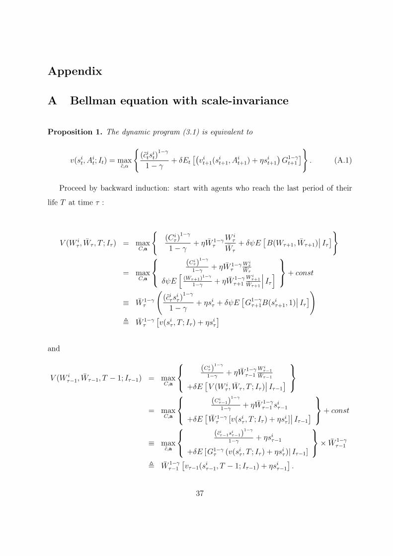
Appendix

A Bellman equation with scale-invariance

Proposition 1. The dynamic program (3.1) is equivalent to

v(sit, A

it; It) = max

c,α

(ci

tsit)

1−γ

1− γ+ δEt

[(vi

t+1(sit+1, A

it+1) + ηsi

t+1

)G1−γ

t+1

]

. (A.1)

Proceed by backward induction: start with agents who reach the last period of their

life T at time τ :

V (W iτ , Wτ , T ; Iτ ) = max

C,a

(Ci

τ )1−γ

1− γ+ ηW 1−γ

τ

W iτ

Wτ

+ δψE[B(Wτ+1, Wτ+1)

∣∣ Iτ

]

= maxC,a

(Ciτ)

1−γ

1−γ+ ηW 1−γ

τW i

τ

Wτ

δψE[

(Wτ+1)1−γ

1−γ+ ηW 1−γ

τ+1W i

τ+1

Wτ+1

∣∣∣ Iτ

] + const

≡ W 1−γτ

((ci

τsiτ )

1−γ

1− γ+ ηsi

τ + δψE[G1−γ

τ+1B(siτ+1, 1)

∣∣ Iτ

])

, W 1−γτ

[v(si

τ , T ; Iτ ) + ηsiτ

]

and

V (W iτ−1, Wτ−1, T − 1; Iτ−1) = max

C,a

(Ciτ)

1−γ

1−γ+ ηW 1−γ

τ−1W i

τ−1

Wτ−1

+δE[V (W i

τ , Wτ , T ; Iτ )∣∣ Iτ−1

]

= maxC,a

(Ciτ−1)

1−γ

1−γ+ ηW 1−γ

τ−1 siτ−1

+δE[W 1−γ

τ [v(siτ , T ; Iτ ) + ηsi

τ ]∣∣ Iτ−1

]

+ const

≡ maxc,a

(ciτ−1si

τ−1)1−γ

1−γ+ ηsi

τ−1

+δE [G1−γτ (v(si

τ , T ; Iτ ) + ηsiτ )| Iτ−1]

× W 1−γ

τ−1

, W 1−γτ−1

[vτ−1(s

iτ−1, T − 1; Iτ−1) + ηsi

τ−1

].

37

Therefore, for any Ait we have

v(sit, A

it; It)W

1−γt = W 1−γ

t ×

maxc,α

(ci

tsit)

1−γ

1− γ+ δEt

[(v(si

t+1, Ait+1; It+1) + ηsi

t+1

)G1−γ

t+1

]

,

which is equivalent to (A.1)

Corollary 2. Households’ optimal consumption and investment policies do not depend on

aggregate wealth.

B Computational Algorithm

The model is solved by iterating on the following steps:

1. Maximization of agents’ utility

2. Simulation of asset returns and the resulting wealth distribution

Maximization

The normalized Bellman equation (A.1) is solved by backward induction. The continu-

ous space of endogenous state variable (agent-specific relative wealth sit ) is discretized using

a grid with 60 points (logarithmically spaced, so that the grid is denser in the lower relative

wealth region, where most of the agents are). For each age and individual wealth state, op-

timal consumption and portfolio choices are found using grid search. I use shape-preserving

Hermite interpolation for the next period’s value function (for the young agents).16

Simulation

At each iteration for each age and aggregate state I draw a large number (10000 for

each age group) relative wealth levels from the initial wealth distribution and interpolate

16Piecewise-cubic Hermite polynomial interpolation (PCHIP) is implemented in the MATLAB curve-fitting toolbox

38

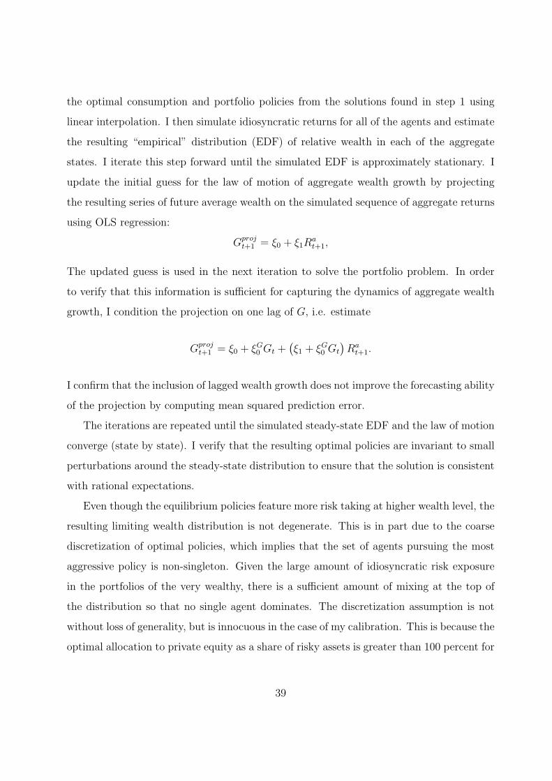
the optimal consumption and portfolio policies from the solutions found in step 1 using

linear interpolation. I then simulate idiosyncratic returns for all of the agents and estimate

the resulting “empirical” distribution (EDF) of relative wealth in each of the aggregate

states. I iterate this step forward until the simulated EDF is approximately stationary. I

update the initial guess for the law of motion of aggregate wealth growth by projecting

the resulting series of future average wealth on the simulated sequence of aggregate returns

using OLS regression:

Gprojt+1 = ξ0 + ξ1R

at+1,

The updated guess is used in the next iteration to solve the portfolio problem. In order

to verify that this information is sufficient for capturing the dynamics of aggregate wealth

growth, I condition the projection on one lag of G, i.e. estimate

Gprojt+1 = ξ0 + ξG

0 Gt +(ξ1 + ξG

0 Gt

)Ra

t+1.

I confirm that the inclusion of lagged wealth growth does not improve the forecasting ability

of the projection by computing mean squared prediction error.

The iterations are repeated until the simulated steady-state EDF and the law of motion

converge (state by state). I verify that the resulting optimal policies are invariant to small

perturbations around the steady-state distribution to ensure that the solution is consistent

with rational expectations.

Even though the equilibrium policies feature more risk taking at higher wealth level, the

resulting limiting wealth distribution is not degenerate. This is in part due to the coarse

discretization of optimal policies, which implies that the set of agents pursuing the most

aggressive policy is non-singleton. Given the large amount of idiosyncratic risk exposure

in the portfolios of the very wealthy, there is a sufficient amount of mixing at the top of

the distribution so that no single agent dominates. The discretization assumption is not

without loss of generality, but is innocuous in the case of my calibration. This is because the

optimal allocation to private equity as a share of risky assets is greater than 100 percent for

39

the wealthiest households, which involves short positions in public equity. Thus a discrete

approximation to the highest share of private equity can be interpreted simply as a short

selling constraint.

C Data description and estimation procedures

Asset holdings: Survey of Consumer Finances (SCF)

I use the 2001 SCF public dataset available from the Federal Reserve Board of Gover-

nors. The survey is representative of the U.S. population and is designed to oversample

the wealthy households. Each household is represented in the dataset by 5 replicates (im-

plicates) constructed in order to compensate for omitted information about households

assets, etc; thus, there are 22210 observations produced from the 4442 households actually

surveyed. Weights are provided to allow aggregation to population totals. For a detailed

discussion of 2001 SCF see, e.g. Kennickell (2003).

The survey contains detailed information on household demographics, income, and asset

holdings. I use the following conventions to define the value of the two main components of

household risky assets, “public equity” and “private equity”. “Risky assets” are assumed

to be comprised of both public equity and private equity (as defined in the appendix), and

also to include corporate and foreign bonds (although their exclusion does not alter the

results); I also consider the definition that includes owner-occupied housing as one of the

risky assets.

Public equity includes directly held stocks plus managed assets such as mutual funds

(except money market funds), retirement plans, annuities, trusts, thrifts, etc. For the

purposes of calculating the households “public equity” investments the following convention

is used in regard to these managed assets: full value if described as mostly invested in stock,

1/2 value if described as split between stocks/bonds or stocks/money market, 1/3 value if

split between stocks/bonds/money market, etc.

Private equity includes the estimated market value of the households’ stakes in private

40

business(es) and/or farm(s), plus loans from household to the business(es), minus loans

from business to household, plus value of personal assets used as collateral; it also includes

the market value of investment real estate, as well as other financial assets that are likely to

be illiquid and/or undiversified, such as oil/gas/mineral leases or investments; association

or exchange membership; futures contracts, stock options, hedge funds; royalties, patents;

non-publicly traded stock, stock with restricted trading rights.

I define “largest risky asset” to be the largest of the following: market value of a

private business interest; value of an investment real estate property; value of “other risky

asset”; value of equity if concentrated in a single stock; average size of a stock holding

for households holding individual stocks (total value of stocks divided by the number of

stocks); value of owner-occupied housing when the latter is included in the definition of

risky assets.

In estimating the cross-sectional distribution of wealth I rank households on their total

assets (instead of net worth) since in the model human wealth is potentially a component

of total wealth, while in the data it is not. Although net worth and total assets are highly

correlated, a number of individuals with high assets (as well as other characteristics corre-

lated with human wealth, such as income and education) also have large debt (especially

mortgage debt). This puts them into lower percentiles of net worth than individuals with

the same level of assets but less debt and potentially lower human capital. Thus, sorts

based on assets should better capture the total wealth ranking, although results based on

net worth are very similar.

Wealth mobility: Panel Study of Income Dynamics (PSID)

I use the PSID wealth supplements for the years 1984, 1989, 1994 and 1999. In order

to obtain estimates of wealth transitions over 10-year periods I track individuals who are

heads of households in 3 successive observations that span a 10-year period. This results

in a sample of 2608 households. I only include households with positive net worth in all

4 observations, which reduces the sample to 1973. This restriction simplifies estimation

41

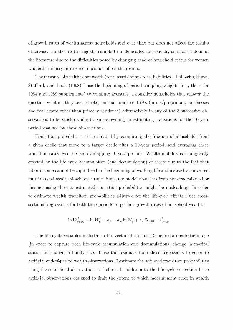
of growth rates of wealth across households and over time but does not affect the results

otherwise. Further restricting the sample to male-headed households, as is often done in

the literature due to the difficulties posed by changing head-of-household status for women

who either marry or divorce, does not affect the results.

The measure of wealth is net worth (total assets minus total liabilities). Following Hurst,

Stafford, and Luoh (1998) I use the beginning-of-period sampling weights (i.e., those for

1984 and 1989 supplements) to compute averages. I consider households that answer the

question whether they own stocks, mutual funds or IRAs (farms/proprietary businesses

and real estate other than primary residence) affirmatively in any of the 3 successive ob-

servations to be stock-owning (business-owning) in estimating transitions for the 10 year

period spanned by those observations.

Transition probabilities are estimated by computing the fraction of households from

a given decile that move to a target decile after a 10-year period, and averaging these

transition rates over the two overlapping 10-year periods. Wealth mobility can be greatly

effected by the life-cycle accumulation (and decumulation) of assets due to the fact that

labor income cannot be capitalized in the beginning of working life and instead is converted

into financial wealth slowly over time. Since my model abstracts from non-tradeable labor

income, using the raw estimated transition probabilities might be misleading. In order

to estimate wealth transition probabilities adjusted for the life-cycle effects I use cross-

sectional regressions for both time periods to predict growth rates of household wealth:

ln W it+10 − ln W i

t = a0 + aw ln W it + azZt+10 + εi

t+10

The life-cycle variables included in the vector of controls Z include a quadratic in age

(in order to capture both life-cycle accumulation and decumulation), change in marital

status, an change in family size. I use the residuals from these regressions to generate

artificial end-of-period wealth observations. I estimate the adjusted transition probabilities

using these artificial observations as before. In addition to the life-cycle correction I use

artificial observations designed to limit the extent to which measurement error in wealth

42

might bias the estimates of transition rates due to spurious volatility. These observations are

obtained by averaging the first and the second pairs of observations: W i86.5 = 1

2(W i

84 + W i89)

, W i96.5 = 1

2(W i

94 + W i99). The transition probabilities are computed for the single implied

period, from mid-1986 to mid-1996. The life-cycle adjustment is applied to the averaged

observations as described above.

Hurst, Stafford, and Luoh (1998) use Shorrock’s index as a measure of wealth mobility.17

For the period 1984-1994 they estimate Shorrock’s index of 0.85. In my extended data the

raw estimate is 0.83, which falls to 0.71 after adjustments for life-cycle and measurement

error. Both the life-cycle adjustment and the averaging procedure reduce the estimates

of wealth mobility, albeit not dramatically. Table VII shows the estimates of Shorrock’s

index of mobility for the three groups of households: all positive net worth households,

stockholders and business owners. It is apparent that while the removal of life-cycle vari-

ation increases persistence, the measurement-error correction has a smaller impact on the

estimates.

17If N is the number of quantiles and tr(P ) is the trace of the corresponding transition matrix P , thenShorrock’s index equals N−tr(P )

N−1 .

43

Table I: Calibration

Technology parameters:

Parameter ValueRisk-free Rate Rf 5%Public Equity Risk Premium E (Ra)−Rf 6%Public Equity Return Volatility σ (Ra) 15%Private Equity Risk Premiums E (Ri)−Rf 6%Private Equity Return Volatility σ (Ri) 45%Systematic risk of private equity βRi,Ra 0.5Probability of good aggregate state Pr

Ra > Rf

23

Preference parameters (status benchmark)

Parameter ValueCurvature of Consumption Utility γ 10Status Utility Weight η 1Subjective Discount Factor β 0.9710

Bequest Utility Weight ψ 1

Initial wealth distributionx 0.005 0.013 0.027 0.053 0.133 0.267 0.533 1.333 2.665 5.330F (x) 0.162 0.187 0.219 0.257 0.328 0.447 0.603 0.819 0.920 0.971

The top panel displays the parameters of asset returns used in calibration, annualized vialogarithmic returns. Public equity return and risk-free rate are based on 10-year CRSPvalue-weighted returns and 10-year Treasury yields, respectively. Private equity return iscalibrated to have the same mean return as public equity and standard deviation threetimes as high. Systematic risk of private equity is captured by its beta (loading) on thepublic equity. Public equity return is approximated by a discrete process with a “good”and a “bad” state. The middle panel displays the range of preference parameter valuesused in simulations. The bottom panel contains a discrete approximation of the wealthdistribution used to initialize the simulated model: for each relative wealth level x thefraction of households with wealth below this level (W i

W≤ x) is given by F (x). This

distribution matches the distribution of households net worth in 2001 SCF (cf. Kennickell(2003)).

44

Table II: Asset holdings and consumption growth volatility

Data Status model CRRA

Equity/total assets 28 25 27Concentrated/total equity 18 18 15Conc. equity/total assets 5 6 4σ

(ln

(Ct+h/Ct

))1.71† 1.85 1.69

σ(

1N

∑ln

(Ci

t+h/Cit

))4.6‡ 4.85 5.33

1N

∑σ

(ln

(Ci

t+h/Cit

))9[ 6.62 6.00

Average portfolio allocations to public and private equity and measures of consumptiongrowth volatility in the U.S. data and in the model.Data: total (public and private) equity as a share of total assets and the share of assetsallocated to concentrated equity (private business or individual stock) for households withpositive equity holdings, obtained from 2001 SCF; consumption growth volatility, annual-ized logarithmic estimates using quarterly expenditures† - aggregate consumption from NIPA, 5-year horizon‡ - individual consumption from CEX, 5-year horizon[ - individual consumption from CEX, quarterlyStatus model: moments simulated for the calibrated model with γ = 10, η = 1.CRRA: moments simulated for the calibrated power utility (η = 0) model with γ = 8.All quantities are in percentage point units.

45

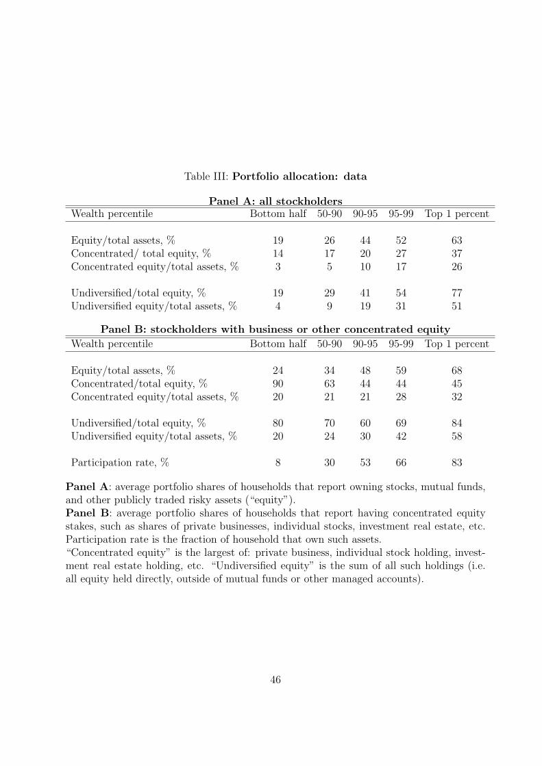
Table III: Portfolio allocation: data

Panel A: all stockholdersWealth percentile Bottom half 50-90 90-95 95-99 Top 1 percent

Equity/total assets, % 19 26 44 52 63Concentrated/ total equity, % 14 17 20 27 37Concentrated equity/total assets, % 3 5 10 17 26

Undiversified/total equity, % 19 29 41 54 77Undiversified equity/total assets, % 4 9 19 31 51

Panel B: stockholders with business or other concentrated equity

Wealth percentile Bottom half 50-90 90-95 95-99 Top 1 percent

Equity/total assets, % 24 34 48 59 68Concentrated/total equity, % 90 63 44 44 45Concentrated equity/total assets, % 20 21 21 28 32

Undiversified/total equity, % 80 70 60 69 84Undiversified equity/total assets, % 20 24 30 42 58

Participation rate, % 8 30 53 66 83

Panel A: average portfolio shares of households that report owning stocks, mutual funds,and other publicly traded risky assets (“equity”).Panel B: average portfolio shares of households that report having concentrated equitystakes, such as shares of private businesses, individual stocks, investment real estate, etc.Participation rate is the fraction of household that own such assets.“Concentrated equity” is the largest of: private business, individual stock holding, invest-ment real estate holding, etc. “Undiversified equity” is the sum of all such holdings (i.e.all equity held directly, outside of mutual funds or other managed accounts).

46

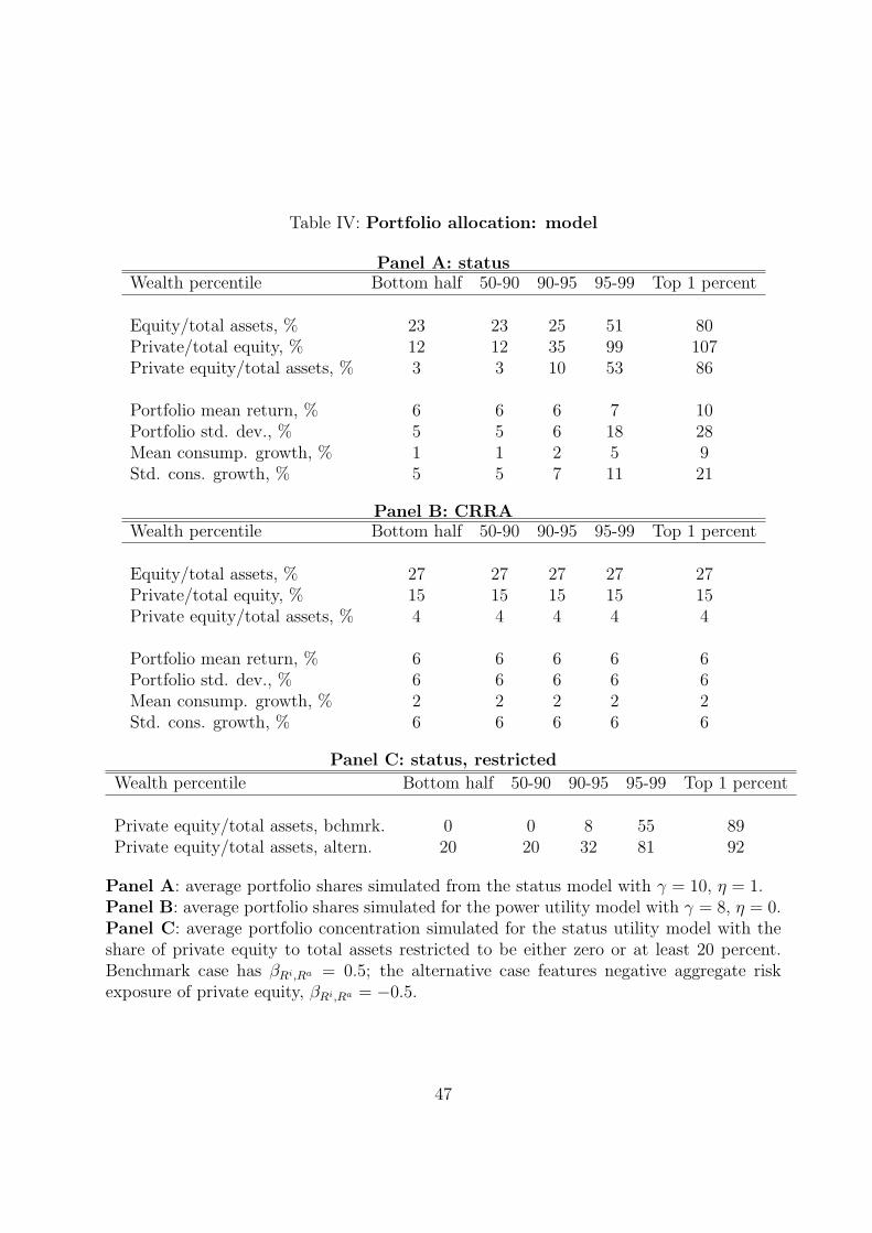
Table IV: Portfolio allocation: model

Panel A: statusWealth percentile Bottom half 50-90 90-95 95-99 Top 1 percent

Equity/total assets, % 23 23 25 51 80Private/total equity, % 12 12 35 99 107Private equity/total assets, % 3 3 10 53 86

Portfolio mean return, % 6 6 6 7 10Portfolio std. dev., % 5 5 6 18 28Mean consump. growth, % 1 1 2 5 9Std. cons. growth, % 5 5 7 11 21

Panel B: CRRAWealth percentile Bottom half 50-90 90-95 95-99 Top 1 percent

Equity/total assets, % 27 27 27 27 27Private/total equity, % 15 15 15 15 15Private equity/total assets, % 4 4 4 4 4

Portfolio mean return, % 6 6 6 6 6Portfolio std. dev., % 6 6 6 6 6Mean consump. growth, % 2 2 2 2 2Std. cons. growth, % 6 6 6 6 6

Panel C: status, restricted

Wealth percentile Bottom half 50-90 90-95 95-99 Top 1 percent

Private equity/total assets, bchmrk. 0 0 8 55 89Private equity/total assets, altern. 20 20 32 81 92

Panel A: average portfolio shares simulated from the status model with γ = 10, η = 1.Panel B: average portfolio shares simulated for the power utility model with γ = 8, η = 0.Panel C: average portfolio concentration simulated for the status utility model with theshare of private equity to total assets restricted to be either zero or at least 20 percent.Benchmark case has βRi,Ra = 0.5; the alternative case features negative aggregate riskexposure of private equity, βRi,Ra = −0.5.

47

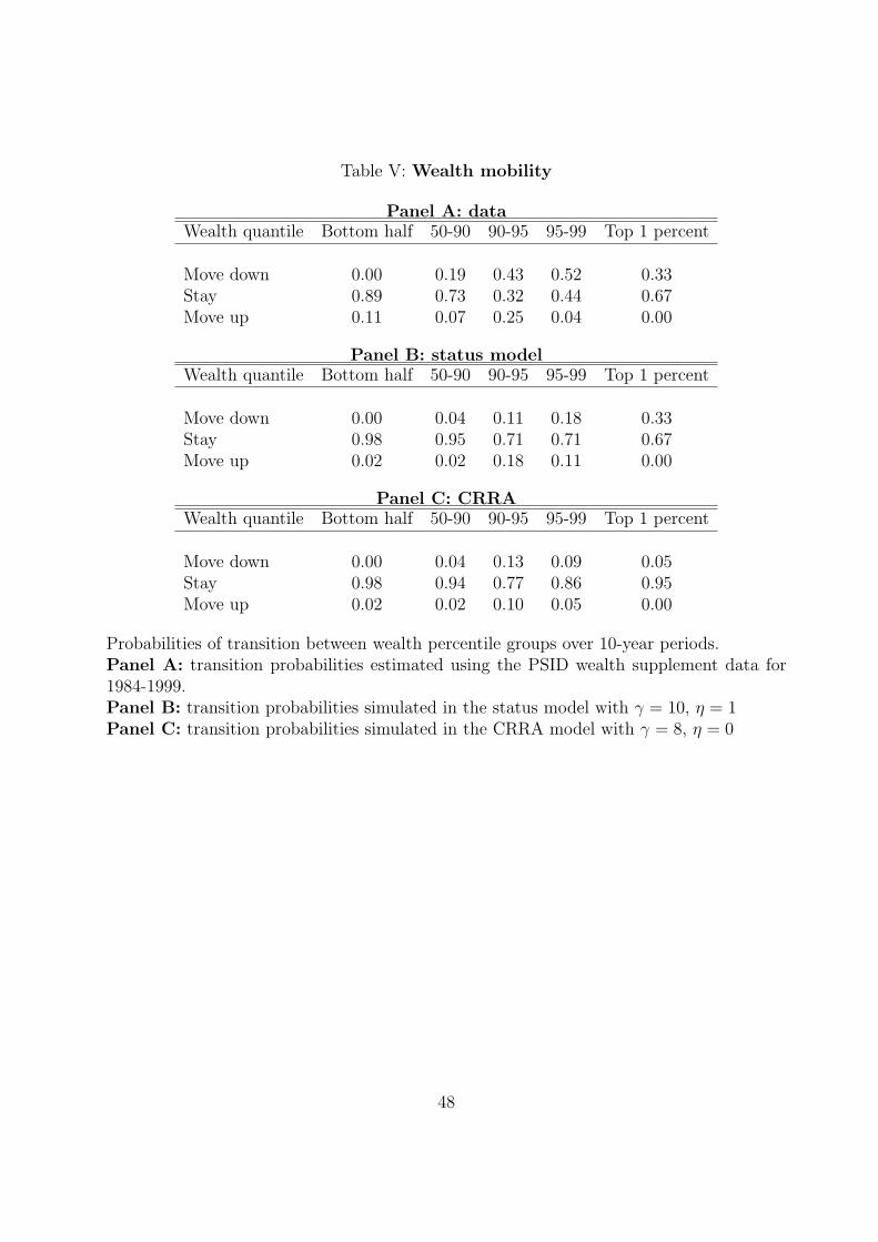
Table V: Wealth mobility

Panel A: dataWealth quantile Bottom half 50-90 90-95 95-99 Top 1 percent

Move down 0.00 0.19 0.43 0.52 0.33Stay 0.89 0.73 0.32 0.44 0.67Move up 0.11 0.07 0.25 0.04 0.00

Panel B: status modelWealth quantile Bottom half 50-90 90-95 95-99 Top 1 percent

Move down 0.00 0.04 0.11 0.18 0.33Stay 0.98 0.95 0.71 0.71 0.67Move up 0.02 0.02 0.18 0.11 0.00

Panel C: CRRAWealth quantile Bottom half 50-90 90-95 95-99 Top 1 percent

Move down 0.00 0.04 0.13 0.09 0.05Stay 0.98 0.94 0.77 0.86 0.95Move up 0.02 0.02 0.10 0.05 0.00

Probabilities of transition between wealth percentile groups over 10-year periods.Panel A: transition probabilities estimated using the PSID wealth supplement data for1984-1999.Panel B: transition probabilities simulated in the status model with γ = 10, η = 1Panel C: transition probabilities simulated in the CRRA model with γ = 8, η = 0

48

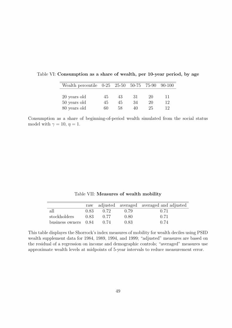
Table VI: Consumption as a share of wealth, per 10-year period, by age

Wealth percentile 0-25 25-50 50-75 75-90 90-100

20 years old 45 43 31 20 1150 years old 45 45 34 20 1280 years old 60 58 40 25 12

Consumption as a share of beginning-of-period wealth simulated from the social statusmodel with γ = 10, η = 1.

Table VII: Measures of wealth mobility

raw adjusted averaged averaged and adjustedall 0.83 0.72 0.79 0.71stockholders 0.83 0.77 0.80 0.71business owners 0.84 0.74 0.83 0.74

This table displayes the Shorrock’s index measures of mobility for wealth deciles using PSIDwealth supplement data for 1984, 1989, 1994, and 1999; “adjusted” measures are based onthe residual of a regression on income and demographic controls; “averaged” measures useapproximate wealth levels at midpoints of 5-year intervals to reduce measurement error.

49

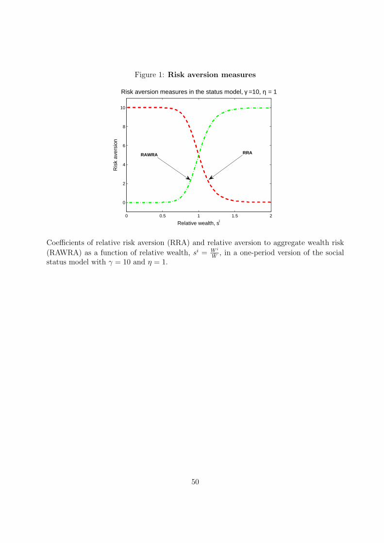
Figure 1: Risk aversion measures

0 0.5 1 1.5 2

0

2

4

6

8

10

Relative wealth, si

Ris

k av

ersi

on

Risk aversion measures in the status model, γ =10, η = 1

RRARAWRA

Coefficients of relative risk aversion (RRA) and relative aversion to aggregate wealth risk

(RAWRA) as a function of relative wealth, si = W i

W, in a one-period version of the social

status model with γ = 10 and η = 1.

50