diversification, growth, and volatility

CHAPTER 3

Diversification, Growth, and Volatility CHRIS PAPAGEORGIOU, NIKOLA SPATAFORA, AND KE WANG

I. INTRODUCTION

Limited diversification in exports and broader economic structure has long been an underlying characteristic of many developing and, in particular, frontier economies. Yet some have shown a remarkable economic transformation, especially over the past two decades. In particular, it has been argued that Emerging Asia, and more recently frontier Asia, have benefited significantly from diversification. This chapter examines this claim with a comprehensive look at the facts, employing newly developed datasets covering diversification in both external trade and domestic production.

The chapter focuses on two key questions. First, is diversification crucial to sustaining growth and reducing volatility? Put differently, does concentration in sectors with limited scope for productivity growth and quality upgrading, such as primary commodities, result in less broad-based and sustainable growth? And does lack of diversification increase exposure to adverse external shocks and macroeconomic instability?

Second, what precisely does diversification, in both external trade and the broader domestic economy, involve? How is it linked to broader structural transformation, including the process of quality upgrading? And which countries and regions have been more successful in promoting diversification?

This chapter is based on ongoing IMF work that aims to inform the policy debate by examining diversification patterns, and the role of diversification in the macroeconomic performance of developing economies, using both cross-country data and case studies.

II. HOW IS DIVERSIFICATION MEASURED?

Measures of economic diversification need to look beyond trade to capture domestic sector diversification and the underlying dynamic process of structural transformation. Trade diversification and domestic diversification are in principle interlinked, the former reflecting diversification in the external sector, and the latter capturing diversification in the domestic production process across sectors. An underlying theme of this chapter is that focusing on the entire structure of production paints a more comprehensive and illuminating picture. Therefore, the two dimensions of diversification are evaluated simultaneously, filling a gap in the existing literature, which has treated them independently. In addition, the analysis focuses on “diversification spurts,” that is, rapid, sustained, significant spells of diversification.

2

Trade diversification can be achieved along several dimensions. First, diversification may occur across either products or trading partners. Second, product diversification may occur through the introduction of new product lines (the extensive margin), or a more balanced mix of existing exports (intensive margin). Finally, product-quality upgrading represents a slightly different notion and is evidenced by higher prices for existing exports. Our main data source for trade is an updated version of the UN–NBER dataset, which harmonizes COMTRADE bilateral trade flow data at the 4-digit Standard International Trade Classification (SITC) (Rev. 1) level.1 However, while the existing literature typically focuses on the post-1988 period, this chapter uses data extending back to 1962. The extended time dimension turns out to be greatly helpful in examining relationships more comprehensively.

Analysis of domestic diversification in frontier economies required construction of a new IMF dataset. This chapter examines diversification in sectoral output and the sectoral allocation of labor using data from existing and new sources. Existing datasets include measures of value added for 28 manufacturing sectors during 1985–2010 (from United Nations Industrial Development Organization 2011; 3-digit ISIC classification); and labor employment shares in nine economy-wide sectors during 1969–2008 (from International Labour Organization 2011; 1-digit classification). It is well known, however, that both of these datasets are quite limited in their coverage of frontier countries. For this reason, a new dataset was constructed, covering 12 economy-wide sectors during 2000–2010, using country data compiled from IMF desk inputs (see below for further discussion).

Appendix 3.1 provides greater details on the diversification indices and quality measures employed in this chapter. Briefly, diversification is measured using the Theil index, which has the advantage of being decomposable into diversification along the extensive and intensive margins. Lower values of the index indicate greater diversification. Quality measures are based on individual products’ unit values (that is, trade prices), but with important adjustments for differences in production costs, as well as for selection bias in the composition of international trade. Appendix 3.2 sets out a full list of the countries and regions analyzed.

III. DIVERSIFICATION, GROWTH, AND VOLATILITY

We start by examining the evidence on the links between diversification and growth. One result stands out: diversification patterns and growth are clearly related, although the relationship displays much heterogeneity. In particular, greater diversification is on average associated with faster subsequent output growth (Error! Reference source not found.). The relationship holds both for the sample as a whole and for Asian countries alone. Adopting a multivariate regression

1 The dataset combines importer- and exporter-reported data from COMTRADE to maximize comprehensiveness, while ensuring internal consistency, using the methodology of Asmundson (forthcoming).

3

approach, output growth remains significantly associated with both initial diversification and initial product quality measures, even after controlling for a variety of standard growth determinants (Table 3.1). This conclusion is in line with the extensive literature, including Singer (1950), Sachs and Warner (1995) on the “natural-resource curse”, and Hausmann and others (2007) on the links between growth and product sophistication.

Figure 3.1. Growth and Diversification, 1962–2010

All Countries Asian Countries

Notes: GDPPC = GDP Per Capita. AZE = Azerbaijan, etc. APD = Asia & Pacific.

Source: COMTRADE, Penn World Table 7.0, IMF staff calculations.

In a similar vein, diversification spurts (defined as in Papageorgiou and Spatafora 2012) are associated with sharp subsequent growth accelerations (defined analogously to diversification spurts). This is especially true for non-fragile frontier countries. Conversely, growth accelerations are associated with subsequent increases in diversification among non-fragile frontier countries.

Next, we examine the links between diversification and volatility. Does diversification serve as a buffer against external shocks? In a related question, are diversification spurts associated with increased macroeconomic stability? The existing literature provides some evidence that countries with more diversified production structures tend to have lower volatility of output, consumption, and investment (Mobarak 2005, Moore and Walkes 2010). Further, product diversification can increase the resilience of frontier economies to external shocks (Koren and Tenreyro 2007).

A key channel is that diversification involves frontier economies shifting resources from sectors where prices are highly volatile and correlated, such as mining and agriculture, to less volatile and correlated sectors, such as manufacturing, resulting in greater stability. And, indeed, the data shows clearly that output volatility diminishes after diversification spurts (Error! Reference source not found.).

AFG

AGO

ALB

AREARG

ARM

AUSAUT

AZE

BDIBEN BFABGD

BGR

BHR

BIH

BLR

BOL

BRA

CAF

CANCHE

CHL

CHN

CIV CMR

COGCOL

CRI

CYP

CZEDEUDNK

DOM

DZAECU

EGY

ERI

ESP EST

ETH

FINFRA

GAB

GBR

GEO

GHA

GIN

GMBGNB

GRC

GTM

HKG

HNDHRV

HTI

HUN

IDNINDIRL

IRN

IRQ

ISRITA

JAMJOR

JPN

KAZ

KEN

KGZKHM

KOR

KWT

LAO

LBN

LBR

LBY

LKALTU

LVA

MAR

MDA

MDG

MEX

MKD

MLIMNG

MOZMRT

MUS

MWI

MYS

NER

NGA

NIC

NLDNOR

NPLNZL

OMNPAKPAN

PERPHL

PNGPOL

PRT

PRY

ROM

RUSRWA

SAUSDN

SEN

SGP

SLE

SLV

SVKSVNSWE

SYRTCD

TGO

THA

TJKTKM

TTOTUNTUR

TZA

UGAUKR

URYUSAUZB

VEN

VNM

ZAF

ZAR

ZMBZWE

-50

51

0R

eal G

DP

PC

Gro

wth

1 2 3 4 5 6Theil Index

AUS

BGD

CHN

HKG

IDN

INDJPN

KHM

KOR

LAOLKA

MNG

MYS

NPLNZL PHL

PNG

SGP

THA VNM

BGDKHM

LAO

MNG

NPL

PNG

VNM

02

46

8R

eal G

DP

PC

Gro

wth

2 2.5 3 3.5 4 4.5Theil Index

Frontier Asia Other APD Countries

4

Figure 3.2. Volatility and Export Diversification

Notes: Episode indicates diversification spurts. The procedure for identifying spurts is based on Berg et al., (2012).

Source: COMTRADE, IMF staff calculations.

IV. PATTERNS OF DIVERSIFICATION

Having established that diversification is indeed linked with macroeconomic performance, we now examine patterns of diversification in greater detail, with a focus on identifying which regions and countries have made greater progress in achieving diversification. Overall, higher income per capita and development are broadly associated with greater trade diversification (Error! Reference source not found..3), at least until an economy reaches advanced-economy status (with GDP per capita of $25,000–$30,000; see also Cadot, Carrere, and Strauss-Kahn 2011). The relationship holds for the sample as a whole. It also holds between and within countries (that is, when the figure is restricted to show the pure cross-sectional or time-series variation); in the latter case, the dataset’s extended time dimension is critical to confirming the relationship.

3.6

3.7

3.8

3.9

4.0

4.1

4.2

4.3

4.4

4.5

Pre-episode Episode Post-episode

Vol

atili

ty o

f GD

P P

er C

apita

,in

per

cent

5

Figure 3.3. Export Diversification and Real GDP Per Capita

Notes: Each observation denotes one country-year combination.


At a regional level, western Europe is the most diversified. However, Emerging and frontier Asia have been rapidly catching up (Error! Reference source not found.). Asia in general shows higher and more rapidly growing diversification than sub-Saharan Africa and Middle East and North Africa, although progress slowed after 1995. Increases in diversification have largely occurred along the extensive margin, that is, through entry into completely new products, although there has also been progress along the intensive margin for Emerging Asia (Error! Reference source not found.). Also, changes in trade diversification over time have been paralleled by decreases in the relative importance of agricultural exports and increases in the relative importance of manufactured exports, especially for Asian countries (Error! Reference source not found.).

Figure 3.4. Export Diversification by Region, 1960–2010: Extensive Margin

12

34

56

The

il In

dex

0 20000 40000 60000Real GDP Per Capita

All Countries Nonparametric FitQuadratic Fit

, , ,

Real GDP per Capita (2000 constant U.S. dollars)

01

23

4T

heil

Ext

ensi

ve

1960 1970 1980 1990 2000 2010Year

Frontier Asia Emerging AsiaSub-Saharan Africa Western EuropeLatin America & Caribbean Middle East & North Africa

6


Figure 3.5. Export Diversification by Region and Period: Intensive Margin


Figure 3.6. Manufacturing Exports Share, by Region and Period


Higher income levels are also associated with increasing diversification across trade partners—at least until advanced-economy status is reached. After 1995, Asia greatly diversified its trade across partners (Error! Reference source not found.). Frontier economies in general, including in sub-Saharan Africa, also have made progress in diversifying their exports across partners. The trend is especially clear when considering the extensive margin, with a significant increase in exports to completely new partners. This is related to ongoing globalization and a clear shift in trade away from the European Union and toward Asia, and China in particular (see also Samake and Yang 2011).

01

23

4T

heil

Inte

nsi

ve

Emerging Asia Frontier Asia Sub-Saharan Africa Western Europe

1965-1970 2006-2010

0.2

.4.6

.8S

har

e o

f Man

ufac

turi

ng E

xpor

ts


1965-1970 2006-2010

7

Figure 3.7. Trade Diversification across Partners over Time


Next, the data also reveal that, within developing countries, greater income per capita is also associated with greater real-sector diversification, that is, diversification in the broader domestic economy. During the 2000s, across all developing countries and within frontier Asia, analysis of six key sectors shows that there was significant real diversification. In particular, the share of agriculture in output declined significantly. The gap was filled largely by nontradables such as construction, wholesale trade, and transportation, rather than by manufacturing (Error! Reference source not found.). That said, there is significant cross-country variation, both in the magnitude of the resource shift out of agriculture and in the precise identity of the sectors that have expanded in its place.

Figure 3.8. Real Sector Share of Frontier Asia, 2000–10

Source: IMF internal data, IMF staff calculations.

01

23

4T

heil

Ind

ex o

n P

art

ner

s


1965-1970 2006-2010

0.2

.40

.2.4

2000 2005 2010 2000 2005 2010 2000 2005 2010

Agriculture Mining Manufacturing

Construction Wholesale trade Transport and communications

Frontier Asia All Developing Countries

Rea

l Sec

tor

Sha

re

year

Graphs by sectorcode

8

V. PATTERNS OF QUALITY UPGRADING

Economic development is underpinned not just by new products and markets, but also by quality improvements to existing products. Producing higher-quality varieties, through more physical- and human-capital intensive production techniques, helps build on existing comparative advantages. It can boost countries’ productivity and export revenues.2 Ongoing work is helping to develop a toolkit to answer key questions, including calculating an economy’s export quality and how it has evolved over time, determining the current potential for quality upgrading, and analyzing whether diversification into new products is a pre-requisite for further quality upgrading. One robust conclusion is that both Emerging Asia and, more recently, frontier Asia have on average enjoyed remarkable success in quality upgrading. That said, significant cross-country variation remains.

Our quality measures are based on individual products’ unit values (that is, trade prices). However, these unit values are adjusted to reflect differences in production costs, as well as selection bias in the composition of international trade. Quality estimates at the country level are then constructed as a geometric value-weighted mean of the quality estimates for individual products. For full details, see Appendix 3.1, as well as Henn, Papageorgiou, and Spatafora (forthcoming). Among other benefits, these quality measures smooth much of the artificial volatility often observed in unit values.

The data suggest some clear patterns. Higher incomes per capita are associated with greater export quality at the country level. The relationship holds both across all goods (Error! Reference source not found.), and (even more clearly) within manufacturing, which has greater scope for differentiation. Quality upgrading is particularly marked as countries evolve from frontier status into middle-income economies.

There is much heterogeneity in quality levels, even when controlling for income per capita. In particular, Emerging Asia has enjoyed immense success in quality upgrading since 1970 (Error! Reference source not found.), whereas frontier Asia only began the process in the early 2000s. Sub-Saharan Africa stands out as producing relatively low-quality goods.

2 See Schott (2004) for an early demonstration that product quality varies significantly and systematically across exporters.

9

Figure 3.9. Quality Index and GDP per Capita in Frontier Asia, 1960–2010


Figure 3.10. Manufacturing Quality Index by Region, 1960–2010


Focusing on Asia, some countries have converged or are continuing to converge to the world frontier. In other cases, convergence seems to have slowed since the mid–1990s (Error! Reference source not found.). Overall, improvements in export quality are associated with growth takeoffs. Hence, Japan converged to the world frontier in the 1970s; Korea’s convergence occurred between the 1970s and the early 1990s; China started its take-off in the late 1980s, and has since been converging very rapidly; and Vietnam’s convergence started in the 1990s. In Malaysia and Thailand, convergence was rapid but appears to have stalled before

0.2

.4.6

.81

Qu

ality

(90

th p

erce

ntile

= 1

)

0 10000 20000 30000 40000Exporter GDP per capita (2000 constant Dollars)

Rest of World Frontier AsiaLowess Fit

Quality across all Exports:Frontier AsiaA

(90

th p

erce

ntile

= 1

)

, , , ,U. S. dollars)

(90

thp

erce

ntile

=1

)Q

ualit

y

10

reaching the world frontier. India seems to be converging but only slowly. Likewise, Bangladesh’s convergence is very slow, particularly given its large catch-up potential.

Figure 3.10. Quality Convergence of Asian Countries, 1960–2010


Crucially, developing countries’ potential for quality upgrading does not appear to be limited by low demand for quality in their existing destination markets. Frontier economies do tend to serve markets that import lower-quality products (Error! Reference source not found.). However, the differences are not substantial enough to act as a constraint on quality upgrading. Indeed, on average, the lower-income the exporter, the greater the gap between its export quality and the average quality of its trade partners’ imports. Likewise, in slow-converging countries, export quality is substantially lower than the average quality of their trade partners’ imports. All this suggests that policy should focus on creating a domestic environment broadly conducive to quality upgrading; lowering barriers to entry into higher-quality export markets constitutes a less urgent priority.

.4.5

.6.7

.8.9

1Q

ualit

y (9

0th

perc

entil

e =

1)

1970 1980 1990 2000 2010Year

Bhutan Bangladesh

Cambodia Laos

Maldives Vietnam

Fast-convergence Frontier Asia

.4.5

.6.7

.8.9

1Q

ualit

y (9

0th

perc

entil

e =

1)

1960 1970 1980 1990 2000 2010Year

Nepal Papua New Guinea

Mongolia

Slow-convergence Frontier Asia

.4.5

.6.7

.8.9

1Q

ualit

y (9

0th

perc

entil

e =

1)

1960 1970 1980 1990 2000 2010Year

China India

Indonesia Malaysia

Sri Lanka Thailand

Fast-covergence Emerging Asia.4

.5.6

.7.8

.91

Qua

lity

(90t

h pe

rcen

tile

= 1

)

1960 1970 1980 1990 2000 2010Year

Fiji Philippines

Slow-convergence Emerging Asia

Fast-Convergence Frontier Asia

Fast-Convergence Emerging Asia

Slow-Convergence Frontier Asia

Slow-Convergence Emerging Asia

11

Figure 3.11. Export Quality by Region, 2009


VI. COUNTRY CASE STUDIES

To obtain robust policy conclusions, it is critical to complement the above cross-country analysis of product diversification and quality upgrading with individual country case studies. To this end, Appendix 3.3 discusses the experience of Bangladesh in more detail, a frontier economy with income per capita well below $1,000, and Vietnam, a country on the threshold of middle-income status. In addition, Pitt et al. (forthcoming) analyze developments in Tanzania, another frontier economy; Angola, the second largest oil exporter in sub-Saharan Africa and a middle-income country still facing significant physical and human capital needs; and Malaysia, an emerging market whose income per capita has grown 20-fold over the past 40 years.

Overall, these case studies provide some tentative evidence in favor of four main themes. First, analyzing the entire structure of production paints a more comprehensive and illuminating picture than focusing purely on external trade. Structural transformation may well be associated with significant diversification of domestic production, including of nontradables. Examining this may shed light on the underlying mechanisms and barriers to further transformation.

Second, diversification and structural transformation are often underpinned by reforms and policy measures that are general in scope. Macroeconomic stabilization is a clear example. But even microeconomic measures are often broad-based, focusing on improving the quantity and quality of infrastructure or essential business services, or on setting up a welcoming environment for foreign investors. It remains an open issue to what extent industry-focused and narrowly targeted measures have historically helped underpin diversification efforts.

Third, effective policy measures come in “waves” and aim at exploiting the evolving comparative advantages of the economy in changing external conditions. The types of reforms

0.6 0.7 0.8 0.9 1

Western Europe

Sub-Saharan Africa

Frontier Asia

Emerging Asia

Export Quality Relative to Destination Markets(World Frontier = 1)

Average Quality Demanded in Destination Countries

Quality Exported

12

underpinning diversification and structural transformation in the early stages of development are different from those required later on and need to be adapted to the external environment the economy faces.

Finally, the frequency with which new products are introduced and the rate at which they grow can indicate potential policy-driven bottlenecks. Limited entry may indicate that barriers deter firms from exporting or experimenting. If survival rates are low, firms may face more obstacles than expected. If surviving firms cannot expand, they may have inadequate access to finance.

VII. CONCLUSIONS

One key message from this chapter and related work is that economic development critically involves diversification and structural transformation—that is, the continued, dynamic reallocation of resources from less productive to more productive sectors and activities. This process involves not just external trade, but the broader economy. Success in this transformation will reduce volatility and accelerate growth.

However, there are major differences across regions and countries in the degree to which they have succeeded in diversifying and transforming their economies. Over an extended period, Asia has on average been particularly successful in diversifying its exports, particularly in comparison with sub-Saharan Africa. Much of the progress has occurred through diversification along the ‘extensive margin,’ that is, through entry into completely new products.

Structural transformation crucially involves changes not only in the type, but also in the quality of goods produced. Emerging Asia has on average benefited significantly from quality upgrading, helping it capitalize on already existing comparative advantages. Yet, the potential for quality upgrading varies by product. Agricultural and natural resources tend to have lower potential for quality upgrading than manufactures. Therefore, for frontier countries, diversification into products with longer “quality ladders” may be a necessary first step before large gains from quality improvement can be reaped.

Overall, development strategies must promote sustained resource reallocation and encourage continued quality upgrading. Ongoing work is focused on identifying the specific bottlenecks to structural transformation. In particular, it will analyze measures of product quality in greater detail and examine what policies are needed to promote diversification and to sustain quality upgrading. That said, case studies of individual countries have already yielded some important lessons. For instance, diversification and structural transformation are often underpinned by reforms and policy measures that are general in scope, rather than industry-focused and narrowly targeted. In addition, the types of reforms underpinning diversification and structural transformation in the early stages of development are different from those required later on.

13

Table 3.1. Growth Regressions with Diversification and Quality Indices

Variables (1) (2) (3) (4) (5) (6) (7) (8) (7) (8)

Lagged GDP -5.363*** -6.027*** -5.898*** -5.897*** -5.604*** -4.886*** -3.882 -7.313*** -5.858** -7.848***(0.439) (0.464) (0.454) (0.471) (1.697) (1.551) (3.488) (2.173) (2.421) (2.326)

Education 0.124*** 0.139*** 0.146*** 0.137*** 0.236** 0.217** 0.203 0.208* 0.124 0.151(0.023) (0.023) (0.023) (0.023) (0.101) (0.100) (0.125) (0.112) (0.123) (0.114)

Investment 3.599*** 3.523*** 3.513*** 3.374*** 4.520*** 4.324*** 4.046** 4.436*** 2.513 3.867***(0.433) (0.429) (0.429) (0.436) (1.428) (1.408) (1.626) (1.401) (1.682) (1.268)

Population Growth -0.053 -0.194 -0.238 -0.118 0.869 0.670 -1.346 -1.759 1.191 0.917(0.229) (0.227) (0.228) (0.227) (0.738) (0.736) (2.749) (2.248) (0.726) (0.745)

Diversification Index -0.608**(0.279)

Quality Index 8.761*** 13.660* -8.572 19.601*(2.124) (6.878) (15.365) (10.970)

Quality Index, Agriculture 9.687*** 21.036** 19.555**(2.348) (8.361) (9.405)

Quality Index, Manufacture 7.646*** 48.638**(2.485) (18.846)

Constant 35.550*** 31.748*** 29.948*** 31.842*** 16.662* 6.508 22.728 0.110 19.448 30.538**(3.720) (3.534) (3.614) (3.570) (9.267) (9.840) (19.191) (18.537) (17.004) (14.384)

Observations 790 789 789 789 75 75 46 46 50 50R-squared 0.234 0.250 0.250 0.241 0.291 0.317 0.295 0.402 0.441 0.456Number of Countries 113 113 113 113 10 10 6 6 7 7

Standard errors in parentheses*** p<0.01, ** p<0.05, * p<0.1

Notes: For Asian country groups, coefficients on diversification index are not significant.Source: IMF staff calculations.

All Countries East Asia South Asia Frontier Asia

Growth Regression, Generalized Least Squares Fixed Effects

14

REFERENCES

Asmundson, Irena. Forthcoming. “More World Trade Flows: An Updating Methodology”, IMF Working Paper.

Cadot, O., C. Carrere, and V. Strauss-Kahn. 2011. “Export Diversification: What’s Behind the Hump?” Review of Economics and Statistic, 93: 590–605.

Hallak, J.C., 2006, “Product Quality and the Direction of Trade,” Journal of International Economics 68: 238–65.

xHarrigan, J., X. Ma, and V. Shlychkov. 2011. “Export Prices of U.S. Firms,” NBER Working Paper No. 17706.

Hausmann, R., J. Hwang, and D. Rodrik. 2007. "What You Export Matters," Journal of Economic Growth, Springer 12 (1) (March): 1–25.

Henn, C., C. Papageorgiou, and N. Spatafora. 2013. “Export Quality in Developing Countries”, IMF Working Paper, International Monetary Fund, Washington, DC.

International Labour Organization (ILO). 2011. Yearbook of Labor Statistics. Geneva: ILO.

Koren, M., and S. Tenreyro. 2007. “Volatility and Development,” Quarterly Journal of Economics 122: 243–87.

Mobarak, A.M. 2005. “Democracy, Volatility, and Economic Development.” Review of Economics and Statistics 87: 348–61.

Moore, W., and C. Walkes. 2010. “Does Industrial Concentration Impact on the Relationship between Policies and Volatility?” International Review of Applied Economics 24: 179–202.

Papageorgiou, C., and N. Spatafora. 2012. “Economic Diversification in LICs: Stylized Facts and Macroeconomic Implications.” IMF Staff Discussion Note 12/13, International Monetary Fund, Washington, DC.

Pitt, A., T.S. Choi, N. Duma, N. Gigineishvili, and S. Rosa. Forthcoming. “Economic Diversification: Experiences and Policy Lessons from Five Case Studies.” IMF Working Paper, International Monetary Fund, Washington, DC.

Sachs, J.D., and A.M. Warner. 1995. “Natural Resource Abundance and Economic Growth,” NBER Working Papers 5398, National Bureau of Economic Research, Cambridge, Mass.

15

Samake, I., and Y. Yang, 2011, “Low-Income Countries’ BRIC Linkage: Are There Growth Spillovers?” IMF Working Paper 11/267, International Monetary Fund, Washington, DC.

Schott, P., 2004, “Across-Product versus Within-Product Specialization in International Trade,” Quarterly Journal of Economics 119: 647–78.

Singer, H., 1950, “US Foreign Investment in Underdeveloped Areas: The Distribution of Gains between Investing and Borrowing Countries.” American Economic Review 40: 473–85.

United Nations Industrial Development Organization (UNIDO), 2011, Industrial Statistics Database. Vienna: UNIDO.

16

APPENDIX 3.1. DEFINITIONS OF MAIN INDICES

A. Herfindahl Index

As a starting point, we measure diversification using the Herfindahl index. The value of the Herfindahl index, for any given country i and time period t, equals the sum of squares of export shares (in total exports), where the summation is across all goods j in the set Jit of categories which the country exports:

HFIit = jJit (Xijt / kJit Xikt)2

where Xijt equals the value of exports by country i of good j at time t. This is an inverse measure of diversification which ranges from maximum of 1 (no diversification: all exports lie in a single category) down to 0 (full diversification: each category contains a negligible fraction of the country's exports).

B. Theil Index

We calculate the overall, within, and between Theil indices following the definitions and methods used in Cadot, Carrere, and Strauss-Kahn (2011). We first create dummy variables to define each product as “Traditional,” “New,” or “Non-traded.” Traditional products are goods that were exported at the beginning of the sample, and non-traded goods have zero exports for the entire sample. Thus, for each country and product, the dummy values for traditional and non-traded remain constant across all years of our sample. For each country/year/product group, products classified as “new” must have been non-traded in at least the two previous years and then exported in the two following years. Thus, the dummy values for new products may change over time.

The overall Theil index is a sum of the within and between components. The between Theil index is calculated for each country/year pair as:

TB = ∑k (Nk/N) (µk/µ) ln(µk/µ)

where k represents each group (traditional, new, and non-traded), Nk is the total number of products exported in each group. µk/µ is the relative mean of exports in each group. The within Theil index for each country/year pair is:

TW = ∑k (Nk/N) (µk/µ) {(1/Nk) ∑i∈Ik (xi/µk) ln(xi/µk)}

17

C. Product Quality

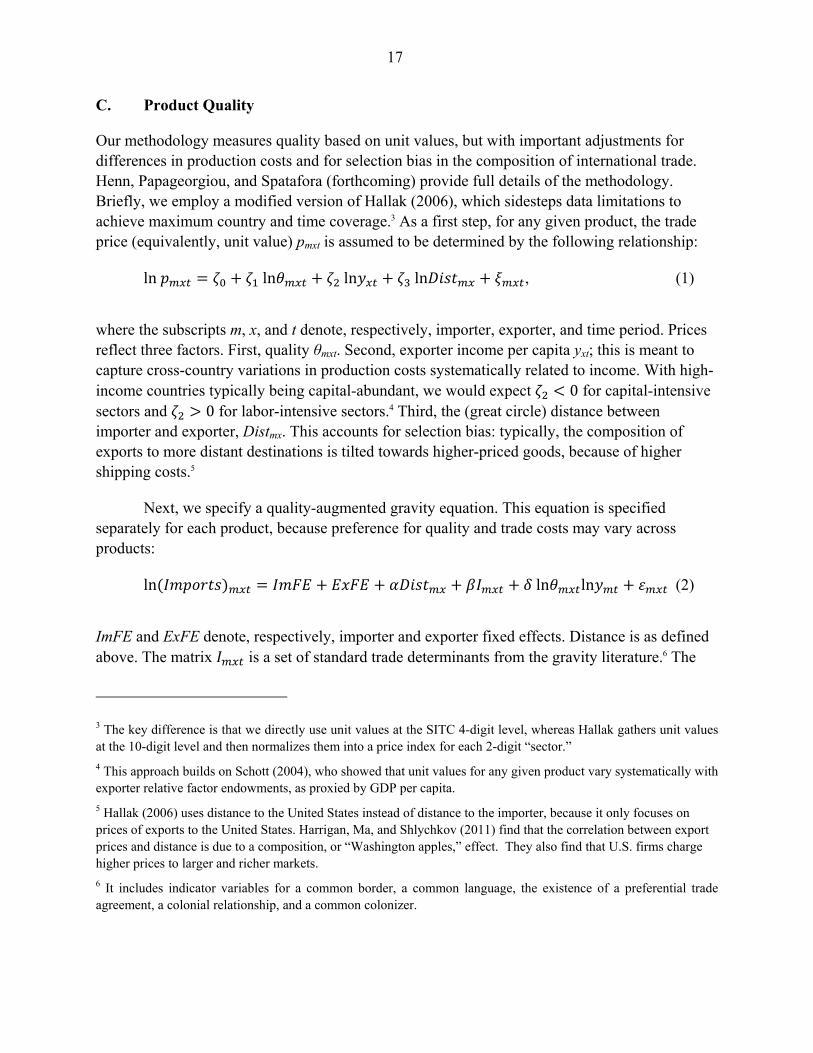
Our methodology measures quality based on unit values, but with important adjustments for differences in production costs and for selection bias in the composition of international trade. Henn, Papageorgiou, and Spatafora (forthcoming) provide full details of the methodology. Briefly, we employ a modified version of Hallak (2006), which sidesteps data limitations to achieve maximum country and time coverage.3 As a first step, for any given product, the trade price (equivalently, unit value) pmxt is assumed to be determined by the following relationship:

ln ln ln ln , (1)

where the subscripts m, x, and t denote, respectively, importer, exporter, and time period. Prices reflect three factors. First, quality θmxt. Second, exporter income per capita yxt; this is meant to capture cross-country variations in production costs systematically related to income. With high-income countries typically being capital-abundant, we would expect 0 for capital-intensive sectors and 0 for labor-intensive sectors.4 Third, the (great circle) distance between importer and exporter, Distmx. This accounts for selection bias: typically, the composition of exports to more distant destinations is tilted towards higher-priced goods, because of higher shipping costs.5

Next, we specify a quality-augmented gravity equation. This equation is specified separately for each product, because preference for quality and trade costs may vary across products:

ln ln ln (2)

ImFE and ExFE denote, respectively, importer and exporter fixed effects. Distance is as defined above. The matrix is a set of standard trade determinants from the gravity literature.6 The

3 The key difference is that we directly use unit values at the SITC 4-digit level, whereas Hallak gathers unit values at the 10-digit level and then normalizes them into a price index for each 2-digit “sector.”

4 This approach builds on Schott (2004), who showed that unit values for any given product vary systematically with exporter relative factor endowments, as proxied by GDP per capita.

5 Hallak (2006) uses distance to the United States instead of distance to the importer, because it only focuses on prices of exports to the United States. Harrigan, Ma, and Shlychkov (2011) find that the correlation between export prices and distance is due to a composition, or “Washington apples,” effect. They also find that U.S. firms charge higher prices to larger and richer markets.

6 It includes indicator variables for a common border, a common language, the existence of a preferential trade agreement, a colonial relationship, and a common colonizer.

18

exporter-specific quality parameter is , which enters interacted with the importer’s income per capita . If 0, then greater income increases the “demand for quality”.

The estimation equation is obtained by substituting observables for the unobservable quality parameter in the gravity equation. Rearranging equation (1) for ln , and substituting into (2), yields:

ln ln ln

2′ln ln 3′ln ln ′ (3)

where , , , and ′ ln .

This equation is estimated separately for each of the 851 products in the dataset, yielding 851 sets of coefficients. We obtain estimates by two stage least squares. is a component of

, so that the regressor ln ln is correlated with the disturbance term ′ . We therefore use ln ln as an instrument for ln ln . Where a unit value for the preceding year is not available (for instance, because the good was not traded), we use the unit value in the closest available preceding year, going back up to 5 years.7

The regression results are used to calculate a comprehensive set of quality estimates. Rearranging (1) and using the estimated coefficients, quality is calculated as the unit value adjusted for differences in production costs and for the selection bias stemming from relative distance:

ln ′ln ′ln ′ln (4)

As is standard, quality and importers’ taste for quality δ are not separately identified.8 The quality estimates are then aggregated into a multi-level database. The estimation yields quality estimates for more than 20 million product-exporter-importer-year combinations. To enable cross-product comparisons, all quality estimates are first normalized by their 90th percentile in the relevant product-year combination. The resulting quality values typically range between 0 and 1.2. The quality estimates are then aggregated, using current trade values as

7 If unit values are not available in any of the preceding five years, the observation is excluded from the estimation.

8 The preference for quality parameter δ will also vary by sector. Therefore, when we aggregate quality estimates across sectors, the aggregation will necessarily also aggregate across these heterogeneous preference for quality parameters.

19

weights, to higher-level sectors (Standard International Trade Classification [SITC] 4-, 3-, 2-, and 1-digit, as well as country-level totals).9 At each aggregation step, the normalization to the 90th percentile is repeated. Aggregations are also produced based on the Broad Economic Categories (BEC) classification, as well as for three broad sectors (agriculture, non-agricultural commodities, and manufactures). To allow for easy comparisons with unit values, the latter are also normalized with the 90th percentile set equal to unity.

9 Changes in the higher-level (including country-level) quality estimates will in general reflect both quality changes within disaggregated sectors, and reallocation across sectors with different quality levels. If the composition of exports is shifting toward product lines characterized by low quality levels, it is quite possible for the quality of any given product to be rising sharply, but country-level quality to rise slowly (or indeed decline).

20

APPENDIX 3.2. REGION DEFINITION

Frontier Asia Emerging Asia Sub-Saharan Africa Western EuropeBangladesh BruneiDarussalam Angola AustriaBhutan China Benin BelgiumCambodia Fiji Botswana CroatiaLaoP.D.R. India BurkinaFaso CyprusMaldives Indonesia Burundi DenmarkMongolia Malaysia Cameroon FinlandMyanmar MarshallIslands CapeVerde FranceNepal Micronesia CentralAfricanRepublic GermanyPapuaNewGuinea Philippines Chad GreeceVietnam SriLanka Comoros Iceland

Thailand Congo, Democratic Republic of IrelandTuvalu Congo, Republic of Israel

Cote d'Ivoire ItalyEquatorial Guinea LuxembourgEritrea MaltaEthiopia NetherlandsGabon NorwayGambia, The PortugalGhana Slovak RepublicGuinea SloveniaGuinea-Bissau SpainKenya SwedenLesotho SwitzerlandLiberia United KingdomMadagascarMalawiMaliMauritaniaMauritiusMozambiqueNamibiaNigerNigeriaRwandaSenegalSeychellesSierra LeoneSomaliaSouth AfricaSudanSwazilandSao Tome and PrincipeTanzaniaTogoUgandaZambiaZimbabwe

21

APPENDIX 3.3. CASE STUDIES

Case studies illustrate lessons from structural transformation at different stages of development. The countries considered include: Bangladesh with income per capita well below $1,000; and Vietnam, a country well on its way to emerging market status. The Vietnam case illustrates lessons from the experiences of countries that have successfully diversified or are successfully diversifying their economies.

Bangladesh illustrates that initial diversification success, to be sustained, requires a combination of further reforms. Diversification in Bangladesh was largely triggered by external factors such as the introductions of the multi-fiber agreement and the generalized system of preferences in the 1970s. These spurred development of the ready-made garments industry. As a result, Bangladesh shifted rapidly away from traditional agricultural and jute products towards manufacturing (Appendix Figure 3.1). Combined with the rise in output from wholesale and retail trade, this contributed to a steady increase in output diversification. Now, however, with ready-made garments accounting for 80 percent of total exports, Bangladesh’s output diversification has seemingly peaked, although as a low cost producer scope remains for further gains through increases in global garment market shares. Attempts to move beyond garments or to increase their quality have been hindered by a lack of supportive reforms. Challenges include poor governance and the high cost of doing business as a result of scarce electricity supplies, severe infrastructure bottlenecks, weak contract enforcement, and expensive credit provision. While such factors did not hinder diversification and inward FDI in the 1990s and early 2000s, they may now be preventing further progress.

Appendix Figure 3.1. Bangladesh: Concentration of Output and Composition of Exports

Bangladesh Output Concentration Composition of Exports

(In percent) (In percent)

Source: Country authorities and IMF staff calculations.

In contrast, Vietnam’s experience shows that “waves” of supportive reforms can sustain diversification and structural transformation. The first wave of reforms during the 1980s opened new areas of activity to the private sector by reducing barriers to entry and expansion. Domestic

22

prices, external trade, and access to foreign exchange were liberalized; the rationing system largely abolished; subsidies significantly cut back; and inflation reduced. In agriculture, individual land-use rights were recognized, production freed from state-set quotas, and collective assets privatized. As a result, agriculture expanded, rising to almost half of total exports in 1995, and also diversified into cash crops, such as coffee and marine and forestry products (Appendix Figure 1.2). In a second wave of reforms during the 1990s, liberalization of foreign direct investment (FDI) helped develop other sectors. Initially, FDI was concentrated in the oil sector, but real estate (including hotels), food processing, and heavy and light industry gained importance. FDI helped Vietnam integrate into emerging global supply chains, and gradually diversify its output and exports from textiles to footwear and electronics. A diversification of trade partners accompanied this product diversification, first from the Soviet Union to Asia, and then towards Europe and the United States.

Appendix Figure 3.2. Vietnam: Diversification of Exports and Composition of GDP

Sources: Country authorities and IMF staff calculations.

Diversification in frontier economies depends crucially on the frequency with which new products are introduced, the likelihood that they will survive, and their growth prospects. Initial trade diversification in frontier economies is mainly driven by entry into new products (the extensive margin). In the above four countries, over 1990–2011, there were significant differences (over time and across countries) in three key measures of the extensive margin: (i) the number of new product varieties introduced in a given year,10 (ii) the survival rates of new varieties, (iii) and the growth rates of surviving varieties. Over time, such differences can cumulate into large differences in overall exports.

Differences in these measures underline the case studies’ different experiences. Vietnam showed significant new entry and reductions over time in the relative importance of incumbent varieties (Appendix Figure 1.3). Vietnam in particular stood out as having a high probability of survival

10 Here, a variety is defined as a specific product exported to a specific country as in Asmundson (forthcoming).

0.15

0.20

0.25

0.30

0.35

0.40

19

90

19

91

19

92

19

93

19

94

19

95

19

96

19

97

19

98

19

99

20

00

20

01

20

02

20

03

20

04

20

05

20

06

20

07

20

08

20

09

20

10

20

11

Agriculture and fisheries

Light industries

Total exports

Vietnam: Export Concentration 1/(Index)

1/ Sum of squares of individual product shares. A lower number indicates greater diversity.

0

2

4

6

8

10

12

14

16

0

5

10

15

20

25

30

35

40

45

50

19

90

19

91

19

92

19

93

19

94

19

95

19

96

19

97

19

98

19

99

20

00

20

01

20

02

20

03

20

04

20

05

20

06

20

07

20

08

20

09

20

10

20

11

Vietnam: Composition of GDP (In percent of total)

Services

Industry and construction

Agriculture ,forestry and

fisheries

GDP per capita (in hundred $, RHS)

23

of new varieties. Bangladesh had less experimentation and also less growth in surviving varieties, accounting for its current, unusually high concentration.

Appendix Figure 3.3. Export Experimentation

Note: BGD = Bangladesh, VNM = Vietnam.


Overall, these case studies provide some tentative evidence in favor of four main themes. First, analyzing the entire structure of production paints a more comprehensive and illuminating picture than focusing purely on external trade. Structural transformation may well be associated with significant diversification of domestic production, including of non-tradables. Analyzing this may shed light on the underlying mechanisms and barriers to further transformation.

Second, diversification and structural transformation are often underpinned by reforms and policy measures that are general in scope. Macroeconomic stabilization is a clear example. But even microeconomic measures are often broad based, focusing on improving the quantity and quality of infrastructure or essential business services, or on setting up a welcoming environment for foreign investors. It remains an open issue to what extent industry-focused and narrowly targeted measures have historically helped underpin diversification efforts.

Third, effective policy measures come in waves and aim at exploiting the evolving comparative advantages of the economy in changing external conditions. The types of reforms underpinning diversification and structural transformation in the early stages of development are different from those required later on and need to be adapted to the external environment the economy faces.

Finally, the frequency with which new products are introduced, and the rate at which they grow, can indicate potential policy-driven bottlenecks. Little entry may indicate that barriers deter firms from exporting or experimenting. If survival rates are low, firms may face more obstacles than expected. If surviving firms cannot expand, they may have inadequate access to finance. This type of analysis suggests directions for further study.

0

2

4

6

8

10

12

14

16

18

20

1990

1991

1992

1993

1994

1995

1996

1997

1998

1999

2000

2001

2002

2003

2004

2005

2006

2007

2008

2009

2010

BGD

VNM

Growth in Varieties Exported(1990 = 1)

0.0

0.1

0.2

0.3

0.4

0.5

0.6

0.7

0.8

0.9

1.0

1990

1991

1992

1993

1994

1995

1996

1997

1998

1999

2000

2001

2002

2003

2004

2005

2006

2007

2008

2009

2010

BGD

VNM

Share of Export Value from Incumbent Varieties

diversification, growth, and volatility

Documents