DIVERSIFICATION, REBALANCING, AND

THE GEOMETRIC MEAN FRONTIER

William J. Bernsteinwbern@mail.coos.or.us

and

David WilkinsonDaveWilk@worldnet.att.net

November 24, 1997

Abstract

The effective (geometric mean) return of a periodically rebalancedportfolio always exceeds the weighted sum of the component geomet-ric means. Some approximate formulae for estimating this effectivereturn are derived and tested. One special case of these formulae isshown to be particularly simple, and is used to provide easily com-puted estimates of the benefits of diversification and rebalancing. Theresults are also used to show how classical Mean-Variance Optimiza-tion may be modified to generate the Geometric Mean Frontier, theanalog of the efficient frontier when the geometric mean is used as themeasure of portfolio return.

1

1 Introduction

The calculation of the true long term, or effective, return is an often ignoredpart of the portfolio optimization process. The case of U.S. common stocksand long term corporate bonds in Table 1 provides a well known example.Here the arithmetic mean return is simply the average of the 69 yearly re-turns, while the geometric mean return is the effective, or annualized, returnover the entire period.

Let us consider an annually rebalanced portfolio consisting of equal parts ofstocks and corporate bonds. Using a simple 50/50 average of the individualreturns one obtains an anticipated portfolio return of 9.00 percent using thearithmetic mean returns and 7.85 percent using the geometric mean returns.In fact, neither is correct: A 50/50 portfolio, rebalanced annually, has anannualized return of 8.34 percent. To complicate matters further, if one hadpurchased the 50/50 mix on January 1, 1926 and not rebalanced, then byDecember 31, 1994 an almost 100 percent stock portfolio would have resulted,with an annualized return of 9.17 percent.

MacBeth (1995) recognized that the uncritical use of a weighted geometricmean results in an anticipated portfolio return which is too low, and sug-gested instead a formulation using the arithmetic mean corrected for vari-ance. For the above example, this gives a return of 8.30 percent, very closeto the actual rebalanced return of 8.34 percent.

The question of whether or not rebalancing benefits portfolio return is morecomplex. Perold and Sharpe (1995) examined the problem from the perspec-tive of historical stock/bill returns and concluded:

In general, a constant-mix (rebalanced) approach will underper-form a comparable buy-and-hold (unrebalanced) strategy whenthere are no reversals. This will be the case in strong bull or bearmarkets, when reversals are small and relatively infrequent, be-cause more of the marginal purchase and sell decisions will turnout to have been poorly timed.

2

We feel that this can only be part of the answer, and that another impor-tant criterion is whether or not the individual assets have similar long termreturn. Common experience demonstrates that rebalancing often yields sig-nificant excess returns when the return differences are small. Contrariwise,rebalancing penalizes the investor when asset return differences are large.

In this paper, we investigate the questions of rebalancing and long term port-folio return in a quantitative manner. We begin by discussing Mean-VarianceOptimization (Markowitz (1952, 1991)) in the context of multi-period port-folio optimization. We then derive two families of approximate PortfolioReturn Formulae, the first of which uses the individual arithmetic means asinput, and the second the geometric means. As a special case of the lat-ter, we obtain a simple approximate formula for the Diversification Bonus,the amount by which the geometric mean return of a rebalanced portfolioexceeds the weighted sum of the individual geometric means. This resultis used to obtain a corresponding formula for the Rebalancing Bonus, theamount by which the return of the rebalanced portfolio exceeds that of thecorresponding unrebalanced one. Lastly, we show how Mean-Variance Opti-mization may be modified to obtain the Geometric Mean Frontier (GMF),the analog of the efficient frontier when the geometric mean is used as themeasure of portfolio return.

Maximization of the geometric mean return has been discussed extensively inthe literature: Latane (1959), Hakansson (1971), Elton and Gruber (1974a,1974b), Fernholz and Shay (1982). However most of this work was concernedwith exact results, the question of whether maximizing the geometric meancan be justified on the basis of utility theory, or with the case of continuoustime rebalancing. We take a more pragmatic and general approach: (a)we will be satisfied with approximate formulae for the portfolio geometricmean, (b) we consider the geometric mean in the context of actual historicaldata with a finite, but arbitrary, rebalancing interval, and (c) we focus onthe entire Geometric Mean Frontier, as opposed to just the single portfoliowhich maximizes the geometric mean.

3

2 MVO – Past and Future

Mean-Variance Optimization (MVO) is designed to produce return/varianceefficient portfolios. The standard Markowitz (1952, 1991) analysis is appli-cable to a single period, and the inputs are the expected returns Ri andcovariance matrix Vij for the individual assets over this period. The latterare related to the standard deviations si and correlation matrix ρij by

Vij = sisjρij , (1)

where ρij = 1 for i = j.

For a portfolio with fraction Xi assigned to asset i, with∑

i Xi = 1, theexpected return R and its variance V are given by

R =∑

i

XiRi , (2)

andV =

∑ij

XiXjVij . (3)

The risk of the portfolio is taken to be the standard deviation s =√

V .

One way to supply the inputs Ri and Vij is to use historical returns, andto assume that the upcoming period will resemble one of the previous Nperiods, each with equal probability 1/N . In this case, the expected returnRi becomes the arithmetic mean return of asset i over the N periods

Ri =1

N

N∑k=1

r(k)i , (4)

where r(k)i is the return of asset i in period k. For the portfolio, the return

R in Eq.(2) becomes the arithmetic mean of the returns of a portfolio whichis rebalanced to the mix specified by the Xi at the beginning of each period

R =1

N

N∑k=1

r(k) , (5)

where r(k) =∑

i Xir(k)i is the return of the rebalanced portfolio in period

k. Note that while the period represented by the returns, e.g. annual or

4

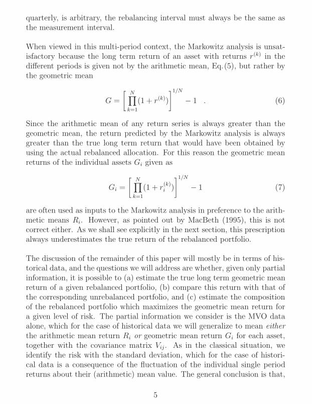
quarterly, is arbitrary, the rebalancing interval must always be the same asthe measurement interval.

When viewed in this multi-period context, the Markowitz analysis is unsat-isfactory because the long term return of an asset with returns r(k) in thedifferent periods is given not by the arithmetic mean, Eq.(5), but rather bythe geometric mean

G =

[N∏

k=1

(1 + r(k))

]1/N

− 1 . (6)

Since the arithmetic mean of any return series is always greater than thegeometric mean, the return predicted by the Markowitz analysis is alwaysgreater than the true long term return that would have been obtained byusing the actual rebalanced allocation. For this reason the geometric meanreturns of the individual assets Gi given as

Gi =

[N∏

k=1

(1 + r(k)i )

]1/N

− 1 (7)

are often used as inputs to the Markowitz analysis in preference to the arith-metic means Ri. However, as pointed out by MacBeth (1995), this is notcorrect either. As we shall see explicitly in the next section, this prescriptionalways underestimates the true return of the rebalanced portfolio.

The discussion of the remainder of this paper will mostly be in terms of his-torical data, and the questions we will address are whether, given only partialinformation, it is possible to (a) estimate the true long term geometric meanreturn of a given rebalanced portfolio, (b) compare this return with that ofthe corresponding unrebalanced portfolio, and (c) estimate the compositionof the rebalanced portfolio which maximizes the geometric mean return fora given level of risk. The partial information we consider is the MVO dataalone, which for the case of historical data we will generalize to mean eitherthe arithmetic mean return Ri or geometric mean return Gi for each asset,together with the covariance matrix Vij . As in the classical situation, weidentify the risk with the standard deviation, which for the case of histori-cal data is a consequence of the fluctuation of the individual single periodreturns about their (arithmetic) mean value. The general conclusion is that,

5

to a good approximation, all three goals above may be accomplished, andthe reason we use the historical perspective is that it enables us to validatethese conclusions. However, the purpose of portfolio theory is, of course, toprovide a basis for decision-making for the future. In the case of the standardsingle period analysis, the input data are necessarily statistical in nature, andthe covariance matrix represents the uncertainty in the returns for the singleupcoming period. However, for multi-period forcasting, two entirely differentviewpoints are possible.

In the first viewpoint, the investor seeks the best course of action over achosen number of upcoming periods, based on the assumption that the hy-pothesized MVO data are actually realized. In this case the problem is con-ceptually no different from that with partial historical data. This viewpointhas no meaning in the case of the usual single period analysis, because if thereturn of each asset is assumed known, then the covariance matrix is zero,and the optimum strategy is just to select the asset with the highest return.However, in the multi-period case, the problem is not so simple. Suppose, aswill usually be the case, that the input returns are chosen to be the geomet-ric mean returns Gi. Firstly, the input covariance matrix represents not theuncertainty in these values, but rather the fluctuations of, and correlationsbetween, the unspecified individual period returns which go to make up thesevalues. Thus there is no contradiction between having both specified valuesfor the returns and a non-zero correlation matrix. Secondly, the computa-tional problem itself is non-trivial. Generally, as we shall see explicitly inSection 6, the rebalanced strategy with the highest geometric mean returnis not to invest 100 percent in the asset with the highest geometric meanreturn; often the highest return strategy is to invest in a diversified portfoliocontaining several of the assets.

The second viewpoint is statistical in nature, and superficially more similarto the conventional single period one. It is, however, necessary to make someadditional hypothesis about the time correlation of the returns. The mostnatural approach, which is in accord with the simplest form of the randomwalk theory of asset price movement, is to asssume that the distribution ofreturns is stationary, i.e. the same in each period, with each period beingindependent of the others. In this case the input return and covariance matrixrepresent the expected value and uncertainty of this unique single perioddistribution. The only new feature is that in the multi-period application we

6

allow the possibilty of specifying the geometric means Gi of this distributioninstead of the arithmetic means Ri. In this viewpoint, the significance of thegeometric mean G (both for the individual assets, and for any rebalancedportfolio of them) is that, as the number of periods becomes large, it becomesincreasingly probable that the actual long term return will lie close to G. Thisproperty is quite general, and is analogous to the observation that if a faircoin is thrown a large number of times, then it becomes increasingly likelythat the fraction of heads will lie close to one half.

Which of these two viewpoints to adopt is perhaps a matter of personaltaste. The actual mathematical development is the same in either case. Wetend to prefer the first viewpoint, because it does not have to make anyindependent assumption about the time correlation of events. For example,if the proposed rebalancing period is annual, then the covariance matrixshould correspond to annual returns; if it is quarterly, then the covariancematrix should correspond to quarterly returns. There is no need for anyrelationship to exist between these two covariance matrices. In the secondviewpoint, however, consistency requires that the two covariance matrices berelated by a factor of four, a relationship which is not necessarily satisfied inreality. For the purposes of this paper, it will certainly be simpler to thinkin terms of the first viewpoint, because there the future is treated in exactlythe same way as the past.

3 Portfolio Return Formulae

In this section we derive and discuss a variety of approximate formulae for thegeometric mean return of a balanced portfolio. These formulae express theportfolio geometric mean in terms of the arithmetic or geometric mean of theindividual assets, together with their covariance matrix. In order to validatethese formulae we will use an actual 9-asset global data set of annual indexreturns over the years 1970-1996. The arithmetic mean return, geometricmean return, and standard deviation of each asset are listed in Table 2; thecorrelation matrix was also computed but is not shown. Note that the assetwith the highest arithmetic mean return (gold) is not the one which has thehighest geometric mean return. In fact, both Japan and U.S. small stocks

7

have higher long term return than gold over this period. Note also that, sincethese are annual returns, the rebalancing period we consider in the examplesis also annual.

We first consider the weighted arithmetic mean and weighted geometric meanas possible portfolio return formulae. The results for the arithmetic meanare shown graphically in the top left plot of Fig. 1. As expected, we seethat the weighted arithmetic mean overestimates the actual portfolio returnin all cases. The corresponding results for the weighted geometric meanare shown in in the top right plot of Fig. 1, where we see that, in contrast,the geometric mean of the portfolio is always underestimated. Neither theweighted arithmetic mean or weighted geometric mean are adequate modelsfor the portfolio geometric mean.

Improved geometric mean formulae may be based on the well known approx-imate relationship between the geometric mean G and arithmetic mean R ofany set of returns

G ≈ R − V

2(1 + R), (8)

where V is the variance of the returns (see, for example, Markowitz (1991)).This formula strictly holds in the limit where the variance is small, but it issurprisingly accurate even outside this range. If, in addition, the arithmeticmean return is small compared to unity then this reduces to

G ≈ R − V

2. (9)

It will be useful in the following to regard both these formulae as specialcases of

G ≈ R − αV

2(1 + βR), (10)

which we will refer to as the (α, β) formula. In this paper we will only considerthe cases (1, 0) and (1, 1), but the general (α, β) case is no more difficult toanalyze than (1, 1), so most of the results will apply to this general case.

A useful feature of the (α, β) formula is that it may be inverted to give

R =2G + αV

1 − βG +√

(1 + βG)2 + 2αβV. (11)

8

When β = 0 this simplifies to

R = G +αV

2. (12)

We first explore the strategy of simply applying the (α, β) formula to theportfolio. We will call this method A(α, β), where the ‘A’ signifies thatthe Arithmetic means Ri of the individual assets are used to construct thearithmetic mean R =

∑i XiRi of the portfolio. The portfolio variance is

obtained fromV =

∑ij

XiXjVij . (13)

The results for methods A(1,0) and A(1,1) are shown in the left column ofFig. 1. It is seen that in both cases there is an improvement over the simpleweighted arithmetic or geometric means. The A(1,1) formula in particulardoes extremely well for the two-asset and randomly selected portfolios, andonly fails for the high return single asset portfolios. Even here, however,the results for both A(1,0) and A(1,1) are much better than those obtainedusing simple weighted arithmetic or geometric means. Note that the weightedarithmetic mean may be considered as the A(0,0) case of A(α, β), so thatthe three plots on the left side of Fig. 1 may be viewed as three cases of thesame formula, with the accuracy impoving from top to bottom.

Two drawbacks of the A(α, β) method are (a) the formula uses the arithmeticmeans of the individual assets rather than their geometric means, and (b)the formula does not give the correct result in the simplest case where theportfolio consists of only a single asset. Both these defects may be remediedby applying the (α, β) formula not only to the portfolio but also to theindividual assets. To do this we first use the inverse relationship on theindividual assets to obtain “pseudo-arithmetic means”

R∗i =

2Gi + αVii

1 − βGi +√

(1 + βGi)2 + 2αβVii

, (14)

and then compute the portfolio arithmetic mean using R =∑

i XiR∗i before

using the (α, β) formula for the portfolio. We call this method G(α, β), wherethe ‘G’ signifies that the geometric means of the individual assets are used asinputs. The results for G(1,0) and G(1,1) are shown in the right column of

9

Fig. 1. It is seen that while the results for the two-asset and random portfoliosare not as good as for the corresponding A(1,0) and A(1,1) cases, the resultsfor the single asset portfolios are now exact. The weighted geometric meanmay be considered as the G(0,0) case of G(α, β), so that the three plots onthe right side of Fig. 1 may be viewed as three cases of the same formula,with the accuracy improving from top to bottom.

In this section we have derived two families A(α, β) and G(α, β) of portfolioreturn formulae, the first of which requires the individual arithmetic meansas inputs and the second their geometric means. While we have focused onthe two cases (1,1) and (1,0), which have some theoretical foundation, it ispossible that, empirically, values other than these might prove to be moreaccurate.

4 The Diversification Bonus

The general G(α, β) method succeeds in expressing the geometric mean re-turn of the portfolio in terms of the geometric mean returns of the individualassets. Though simple to evaluate numerically, the expession is rather cum-bersome and not very intuitive. However, when β = 0 the expression simpli-fies because the inverse relation in Eq.(11) reduces to the simpler Eq.(12).In the following, we will also set α = 1, though the case of general α is nomore difficult. In this case, G(1, 0), we find

G ≈ ∑i

XiGi +1

2

∑

i

XiVii −∑i,j

XiXjVij

. (15)

The analogous result in the limit of continuous time rebalancing has beenobtained previously by Fernholz and Shay (1982), who showed that it is exactwhen the prices follow geometric Brownian motion. A different form of thesame result may be obtained by using

∑i Xi = 1 in the first term inside the

parentheses and symmetrizing to give

G ≈ ∑i

XiGi +∑i<j

XiXj

(Vii

2+

Vjj

2− Vij

), (16)

where the sum is over all pairs i and j with i < j.

10

This form of the G(1, 0) formula has been obtained previously using an em-

pirical argument1. The interesting feature of this formula, not shared bythe general G(α, β) with β 6= 0, is that it separates into two terms, the firstof which depends only on the geometric mean returns, and the second onlyon the covariance matrix. Eq.(16) demonstrates that, for given values ofthe individual returns Gi, it is possible for the portfolio return G to be anincreasing function of the volatility (standard deviation) of the individualassets. In particular, if all the off-diagonal elements of the correlation matrixρij are zero or negative, then the portfoloio return is an increasing functionof each of the standard deviations si. The benefits of a rebalancing strategybecome much greater for assets which are volatile and poorly correlated.

Let us write Eq.(16) in the form

G − ∑i

XiGi ≈∑i<j

XiXj

(Vii

2+

Vjj

2− Vij

). (17)

We will refer to the left side of Eq.(17), which is always positive, as the

Diversification Bonus2, because it represents the effective return in excessof that calculated from the simple combination of the individual geometricmean returns. The right hand side of Eq.(17) provides an approximation tothis quantity which is expressed solely in terms of the covariance matrix ofthe assets. On the left side of Fig. 2 we compare the approximate formula,Eq.(17), with the true value of G − ∑

i XiGi. It is seen that some of theportfolios have a Diversification Bonus in excess of 200 basis points. AlthoughEq.(17) tends to overestimate the precise value of G−∑

i XiGi, as we wouldexpect from the plot for formula G(1,0) in Fig. 1, it does a good job ofpredicting which portfolios will have significant Diversification Bonus. Onthe right side of Fig. 2 we show the corresponding plot for the case G(1,1);while this formula does not lead to a simple form like Eq.(17), it gives abetter approximation to the true Diversification Bonus, as again we wouldexpect from Fig. 1.

11

5 The Rebalancing Bonus

The weighted geometric mean∑

i XiGi provides a naive estimate of effec-tive portfolio return, but it does not correspond to the return obtainable byany particular investment strategy. A more meaningful comparison is thatbetween the return G of the rebalanced portfolio and the return G′ of thecorresponding unrebalanced portfolio. The latter is given by

G′ =

[∑i

Xi(1 + Gi)N

]1/N

− 1 . (18)

Subtracting Eq.(18) from Eq.(16) we obtain

G − G′ ≈[∑

i

Xi(1 + Gi)

]−

[∑i

Xi(1 + Gi)N

]1/N

+∑i<j

XiXj

(Vii

2+

Vjj

2− Vij

). (19)

We will refer to the left side of Eq.(19) as the Rebalancing Bonus3, becauseit represents the difference between the returns of the rebalanced and un-rebalanvced portfolios. In the approximation on the right hand side, theterm on the first line always gives a negative contribution, thus favoring theunrebalanced portfolio. This term is large when the differences between thelong term returns Gi are large, and vanishes when all the returns Gi are thesame. The term in the second line always gives a positive contribution, thusfavoring the rebalanced portfolio. This term is large when the individualassets have large variances, and low or negative correlation.

For the data set considered in Section 3, it is found that the majority ofportfolios perform better when rebalanced. This is illustrated in the left sideof Fig. 3, in which we compare Eq.(19) with the true value of G − G′. Itis seen that the great majority of the portfolios have positive values for thisquantity. Examination of the data underlying Fig. 3 shows that the onlyportfolios giving a significant negative value are 50/50 2-asset portfolios inwhich one of the assets is Treasury Bills. This is in accordance with the abovediscussion – only in this case is the return difference sufficient to overcome thesecond term in Eq.(19). We also see that the approximate formula in Eq.(19)

12

always gives the correct sign for G−G′, although it tends to overestimate theprecise benefit of rebalancing, as we would expect from the plot for formulaG(1,0) in Fig. 1. On the right side of Fig. 3 we show the correspondingplot for the case G(1,1); while this formula does not lead to the simplifyingseparation of Eq.(19), it gives a better model value for G − G′, as again wewould expect from Fig. 1.

The first line in Eq.(19) vanishes when all the returns Gi are equal, but thereis no simple way to express Eq.(19) in terms of return differences alone. Overa long enough time period, however, the unrebalanced portfolio becomesdominated by the highest return asset, independent of the initial allocation,and we obtain

G′ ≈ Gmax , (20)

where Gmax = maxi Gi is the maximum return obtainable from any unrebal-anced portfolio. In this case the Rebalancing Bonus becomes

G − G′ ≈ ∑i

Xi(Gi − Gmax) +∑i<j

XiXj

(Vii

2+

Vjj

2− Vij

). (21)

In this case it is clear that if all the Gi are the same, then the rebalancedportfolio is always superior to the unrebalanced one.

6 The Geometric Mean Frontier

When used with historical data, the traditional Markowitz efficient frontierdesignates those portfolios with greater (arithmetic mean) return than anyother with the same or lesser risk, and lesser risk than any other with thesame or greater return. The Markowitz return R and risk s are defined by

R =∑

i

XiRi , (22)

ands2 =

∑ij

XiXjVij . (23)

In this section we show that it is possible to modify the MVO analysis toconstruct the analogous efficient frontier when the geometric mean is used

13

instead of Eq.(22) as the measure of return, while keeping Eq.(23) as themeasure of risk. More precisely, we show that this Geometric Mean Frontier(GMF) may be computed exactly when any of the approximate geometricmean formulae A(α, β) or G(α, β) of Section 3 is used, and that in eachcase the efficient frontier so obtained provides a good approximation to theefficient frontier of the true geometic mean, the latter being obtained usingthe optimization feature of a standard spreadsheet package4.

In each of the methods A(α, β) or G(α, β), the portfolio geometric mean hasthe form

G = R − αs2

2(1 + βR), (24)

where R and s are given in terms of the individual assets by expressions ofthe form of Eqs. (22) and (23). The only difference between the cases is thatfor A(α, β) the individual returns Ri are the true arithmetic mean returns,while for G(α, β) the Ri are pseudo-arithmetic means R∗

i given in Eq.(14).To simplify the notation we will omit the superscript in this latter case. Also,in this section we will use the symbol ‘G’ to denote the appropriate modelgeometric mean, so that Eq.(24) should be thought of as a definition, ratherthan as an approximate relation for the true geometric mean.

The key to the analysis is to consider an auxiliary classical Markowitz op-timization which uses the arithmetic means as inputs. We emphasize thateven in the case of G(α, β), which expresses the portfolio geometric meanin terms of the individual geometric means, the inputs to this auxiliaryMarkowitz problem are the individual pseudo-arithmetic means, not the ge-ometric means.

We begin by generalizing an argument first given by Elton and Gruber (1974b)to show that any portfolio which is (G, s) efficient must also be Markowitz(R, s) efficient. For any (α, β), the geometric mean expression in Eq.(24) hasthe properties

∂G

∂R> 0 , (25)

∂G

∂s< 0 . (26)

Suppose that (R1, s1), with corresponding geometric mean G1, is not Marko-

14

witz efficient. Then there exists a portfolio (R2, s2), with correspondinggeometric mean G2, with either R2 > R1 and s2 ≤ s1, or R2 ≥ R1 ands2 < s1, or both. In either case it follows from Eqs. (25) and (26) thatG2 > G1 and s2 ≤ s1. Thus no portfolio which is not Markowitz efficientcan be geometric mean efficient; equivalently, every geometric mean efficientportfolio must be Markowitz efficient. Note that the above argument doesnot assume the existence of a continuous path of portfolios between portfolios1 and 2.

The Markowitz efficient frontier extends between the minimum variance port-folio at s = smin and the maximum return portfolio at s = smax. For each sin the range smin ≤ s ≤ smax the frontier gives a corresponding return Rf (s),and this function Rf(s) has the properties

dRf

ds> 0 , (27)

d2Rf

ds2< 0 . (28)

Let us define Gf(s) by evaluating Eq.(24) on the Markowitz frontier, i.e.

Gf(s) = Rf (s) − αs2

2(1 + βRf(s)). (29)

From the above discussion, the (G, s) efficient frontier must be a sub-graphof the graph of Gf(s). Thus the multi-dimensional space of candidate (G, s)efficient portfolios has been reduced to a one-dimensional one.

It can be shown using Eqs. (27) and (28) that, under very reasonable as-sumptions on the nature of the function Rf (s), the function Gf(s) can haveonly one maximum in the range smin ≤ s ≤ smax. In general there are threepossibilities: (a) the maximum occurs at smin; in this case the geometricmean frontier consists of a single portfolio, the minimum variance portfolio,(b) the maximum occurs at smax; in this case the entire Markowitz frontieris geometric mean efficient, or (c) the maximum occurs at some intermediatepoint; in this case only that part of the Markowitz frontier to the left of thismaximum is geometric mean efficient. This third possibility is the one whichoccurs for our chosen example.

15

The portfolio with the maximum geometric mean may be algorithmicallydetermined by starting from the minimum variance portfolio at s = smin andmoving to the right along the Markowitz frontier until the correspondingG = Gf (s) first decreases. The standard MVO output consists of a set of“corner portfolios” located on the Markowitz frontier, between each adjacentpair of which the frontier is obtained by linear combination. The task oftesting for a maximum of Gf (s) between any pair of corner portfolios iseasily accomplished by using the composition, rather than the risk, as theindependent variable. Since Gf(s) has only one maximum, a maximum willbe found in at most one corner interval, and that interval will always be onewhich is adjacent to the corner portfolio with the highest geometric meanreturn.

We examine the validity of these ideas using the same 9-asset data set con-sidered in Section 3. In Fig. 4 we plot the Markowitz efficient frontier, andassociated model and actual geometric means, for the four cases A(1,0),G(1,0), A(1,1) and G(1,1). The result of the exact spreadsheet optimizationof the true geometric mean is also shown. The four cases are qualitativelyvery similar. In each, the maximum of the geometric mean (model or actual)occurs at an intermediate value of risk; the Markowitz frontier greatly over-estimates the true reward of increasing risk. Note also that, while the modelreturns in the four cases show some differences, as we would expect from thediscussion of Section 3, the true geometric mean evaluated on the frontier isfor each case in excellent agreement with the result of the full optimizationof the true geometric mean.

In Table 3 we present in tabular form three portfolios on the efficient fron-tier for each of the the four methods A(1,0), G(1,0), A(1,1) and G(1,1),together with the exact numerical result. Table 3a shows the portfolio whichmaximizes the model geometric mean. We see that the composition of theoptimum portfolio is in all four model cases in reasonable agreement withthe exact one, and that despite the fact that the corresponding model ge-ometric means are somewhat different from each other, the true geometricmeans are close not only to each other, but also to the correct maximumof 16.85 percent. An even better result may be obtained by choosing theoptimal portfolio to be that which maximizes (over the Markowitz frontier)the true geometric mean return, rather than the model geometric mean. Thecorresponding results are shown in Table 3b. In this case it is seen that

16

the portfolio compositions are in closer agreement with the exact ones, andthat, to the quoted precision, all four approximate methods obtain the cor-rect maximum geometric mean of 16.85 percent. It is also possible to usethe efficient frontier of the auxiliary Markowitz problem to determine thegeometric mean efficient portfolio corresponding to a given value of risk s, ormodel geometric mean G, or true geometric mean. As an example, we showin Table 3c the results obtained by fixing s to be 10.0 percent. Again, we seethat the portfolio compositions are in good agreement with the exact ones,and that the values for the true geometric mean reproduce the exact valueof 13.54 percent to within at most one basis point.

The extremely close agreement when the true geometric mean return is usedfollows from a general result of perturbation theory, namely that when theobjective function of an optimization is perturbed by a small amount, thechange in the value of the unperturbed objective function in going to the newmaximum is second order in the perturbation. The excellent agreement isthus due to the fact that all the A(α, β) and G(α, β) formulae are reasonableapproximations to the true geometric mean.

The net result of this section is that, although the A(α, β) and G(α, β) for-mulae are not perfect models for the true geometric mean, in each case theefficient frontier of the auxiliary Markowitz problem does contain portfolioswhose true geometric mean return is extremely close to the real maximum,either in an absolute sense, or when the risk is specified to take a given value.Thus, finding the optimal geometric mean portfolio becomes a tractable nu-merical task, even for a large number of assets, because the space of candidateportfolios becomes one-dimensional.

7 Discussion

This paper contains four significant results, each of which can be easily usedby investors who are able to express their data in the form commonly usedby a standard Mean-Variance Optimization package – namely the arithmeticmean return Ri or geometric mean return Gi of each asset, and the covariancematrix Vij between the assets. These results are:

17

1. Two families A(α, β) and G(α, β) of approximate Portfolio Return For-mulae for estimating the geometric mean return of a rebalanced portfo-lio. The family A(α, β) requires the arithmetic means of the individualassets, and G(α, β) the geometric means.

2. For the case G(1,0), a particularly simple approximate formula, Eq.(17),for the Diversification Bonus, the amount by which the portfolio ge-ometric mean exceeds the weighted sum of the individual geometricmeans.

3. A corresponding approximate formula, Eq.(19), for the RebalancingBonus, the difference between the returns of the rebalanced and unre-balanced portfolios.

4. An extension of classical Mean-Variance Optimization which allowsconstruction of a good approximation to the entire Geometric MeanFrontier (GMF), and in particular that portfolio which maximizes thegeometric mean return.

The validity of these results was demonstrated using historical data. Thechosen data set, containing as it does some extremely volatile assets, is astringent test of the theory; much more accurate results would be obtainedby applying the methodology to a less volatile group of assets, such as dif-ferent classes of U.S. stocks and bonds. However we believe that the majorapplication of these ideas is precisely in generating diversified portfolios ofvery volatile assets, because there lies the greatest potential benefit of di-versification and rebalancing, and of optimizing specifically for long termreturn.

The formalism presented here is not limited to annual returns, but may beapplied for any rebalancing period. For example, if the rebalancing period isquarterly, then the arithmetic and geometric mean returns should be quar-terly returns, and the covariance matrix should be constructed from the his-torical quarterly returns. If desired, the resulting portfolio return G may beconverted to annual return at the end of the calculation. The methodologymay thus be used to investigate the effect of varying the rebalancing period.

While our focus has been on the analysis of historical data, the goal of port-folio theory is of course to generate optimal strategies for the future. In

18

the historical case, the simplest and most accurate of the MVO methods pre-sented here is to use the arithmetic means as inputs to the optimizer, and usethe A(1,1) formula or, even better, the actual returns, to evaluate the portfo-lio geometric mean along the frontier. This will always generate an excellentapproximation to the true Geometric Mean Frontier. There is no need toconsider the G(α, β) formulae and pseudo-arithmetic means. However, whenconsidering long term future strategies the situation is very different (for theinterpretation of the formalism in this situation, recall the discussion at theend of Section 2). Here it is unlikely that investors will simply adopt the his-torical geometric mean, arithmetic mean and covariance matrix. At the least,they will provide their own estimate of return, and this return will be the ef-fective long term, i.e. geometric mean, return. In this case the G(α, β) familyof Portfolio Return Formulae, and the associated use of pseudo-arithmeticmeans as MVO inputs, become indispensible. The G(1,1) formula will givethe best results when used in the MVO analysis, while the simpler G(1,0)formula can provide good intuitive understanding of the performance of dif-ferent portfolio allocations. We emphasize once again that simply using theindividual geometric means as MVO inputs always underestimates the truelong term return, even when the input data for the individual assets proveto be correct.

Notes

1. Bernstein, William J., “The Rebalancing Bonus: Theory and Practice”,Efficient Frontier (September 1996), http://www.coos.or.us/˜wbern/ef.

2. Previously (see Note 1) the left side of Eq.(17) was termed the Rebal-ancing Bonus; here we use this expression for the left side of Eq.(19).

3. See Note 2.

4. Quattro Pro, Version 6.0.

19

References

[1] Elton, Edwin J., and Martin J. Gruber, 1974a. “On the Optimality ofSome Multi-Period Selection Criteria”, Journal of Business, Vol. 47, No.2, pp. 231-243.

[2] Elton, Edwin J., and Martin J. Gruber, 1974b. “On the Maximizationof the Geometric mean with Lognormal Return Distribution”, Manage-ment Science, Vol. 21, No. 4, pp. 483-488.

[3] Fernholz, Robert, and Brian Shay, 1982. “Stochastic Portfolio Theoryand Stock Market Equilibrium”, Journal of Finance, Vol. 27, No. 2, pp.615-624.

[4] Hakansson, Nils H., 1971. “Capital Growth and the Mean-Variance Ap-proach to Portfolio Selection”, Journal of Financial and QuantitativeAnalysis, Vol. VI, No. 1, pp. 517-558.

[5] Latane, Henry A., 1959. “Criteria for Choice Among Risky Ventures”,Journal of Political Economy (April).

[6] MacBeth, James D., 1995. “What’s the Long-Term Expected Return toYour Portfolio?”, Financial Analysts Journal (September/October).

[7] Markowitz, Harry M., 1952. “Portfolio Selection”, Journal of Finance,Vol. 3, No. 1.

[8] Markowitz, Harry M., 1991. Portfolio Selection: Efficient Diversifica-tion of Investments, 2nd edition, Basil Blackwell Ltd, Cambridge, Mas-sachusetts.

[9] Perold, Andre F. and William F. Sharpe, 1995. “Dynamic Strategies forAsset Allocation”, Financial Analysts Journal (January/February).

20

Arithmetic Geometric Standardmean mean deviation

STOCKS 0.1216 0.1019 0.2020BONDS 0.0583 0.0551 0.0850

Table 1: Arithmetic mean, geometric mean and standard deviation forU.S. Common Stocks and Long Term Corporate Bonds for 1926-94.

21

Arithmetic Geometric Standardmean mean deviation

S&P 500 0.1346 0.1227 0.1585SMALL US (9-10) 0.1659 0.1415 0.2293EAFE-E 0.1486 0.1305 0.2095EAFE-PXJ 0.1641 0.1226 0.3084JAPAN 0.1895 0.1454 0.3368GOLD 0.2014 0.1370 0.429920 Y TREAS 0.0989 0.0927 0.11895 Y TREAS 0.0950 0.0928 0.0686T BILL 0.0692 0.0688 0.0267

Table 2: Annual arithmetic mean return, geometric mean return, and stan-dard deviation for nine asset classes over the period 1970-1996. S&P 500,U.S. 9-10, and Treasury security retrurns from SBBI, Ibbotson and Asso-ciates. MSCI-EAFE-E, MSCI-EAFE-PXJ and MSCI Japan from MorganStanley. Gold from Morningstar Inc, and Van Eck Group.

22

A(1,0) G(1,0) A(1,1) G(1,1) ExactSMALL US (9-10) 0.3530 0.2190 0.3049 0.2204 0.2767JAPAN 0.3385 0.3778 0.3633 0.3866 0.3533GOLD 0.3085 0.4032 0.3318 0.3931 0.3699Markowitz return 0.1848 0.2056 0.1863 0.1946 0.1874Standard deviation 0.1969 0.2242 0.2047 0.2228 0.2120Model geometric mean 0.1655 0.1805 0.1686 0.1738 0.1685True geometric mean 0.1681 0.1683 0.1684 0.1684 0.1685

(a) Maximum model geometric mean

A(1,0) G(1,0) A(1,1) G(1,1) ExactSMALL US (9-10) 0.2649 0.2769 0.2649 0.2732 0.2767JAPAN 0.3839 0.3526 0.3839 0.3623 0.3533GOLD 0.3512 0.3705 0.3512 0.3646 0.3699Markowitz return 0.1874 0.2027 0.1874 0.1925 0.1874Standard deviation 0.2120 0.2120 0.2120 0.2119 0.2120Model geometric mean 0.1650 0.1803 0.1685 0.1736 0.1685True geometric mean 0.1685 0.1685 0.1685 0.1685 0.1685

(b) Maximum true geometric mean

A(1,0) G(1,0) A(1,1) G(1,1) ExactSMALL US (9-10) 0.2407 0.2218 0.2407 0.2270 0.2396EAFE-E 0.0172 0.0096 0.0172 0.0186 0.0166JAPAN 0.1402 0.1445 0.1402 0.1414 0.1400GOLD 0.1290 0.1403 0.1290 0.1359 0.13035 Y TREAS 0.4729 0.4839 0.4729 0.4772 0.4736Markowitz return 0.1399 0.1461 0.1399 0.1416 0.1399Standard deviation 0.1000 0.1000 0.1000 0.1000 0.1000Model geometric mean 0.1349 0.1411 0.1355 0.1372 0.1354True geometric mean 0.1354 0.1353 0.1354 0.1354 0.1354

(c) Portfolio with standard deviation s = 0.10

Table 3: Three portfolios on the Markowitz frontier for each of the fourcases A(1,0), G(1,0), A(1,1) and G(1,1). The final column shows the cor-responding exact result.

23

0.08

0.12

0.16

0.08 0.12 0.16

A

0.08

0.12

0.16

0.08 0.12 0.16

A(1,0)

0.08

0.12

0.16

0.08 0.12 0.16

A(1,1)

0.08

0.12

0.16

0.08 0.12 0.16

G

0.08

0.12

0.16

0.08 0.12 0.16

G(1,0)

0.08

0.12

0.16

0.08 0.12 0.16

G(1,1)

Figure 1: Cross-plot of model (vertical axis) against actual (horizontalaxis) geometric mean return, for weighted arithmetic mean (A), weightedgeometric mean (G), and formulae A(1,0), G(1,0), A(1,1) and G(1,1). Eachplot shows the 9 single-asset portfolios (squares), the 36 two-asset portfolioswith 50-50 mix, and 25 randomly generated portfolios.

24

0

0.01

0.02

0.03

0.04

0 0.01 0.02 0.03 0.04

G(1,0)

0

0.01

0.02

0.03

0.04

0 0.01 0.02 0.03 0.04

G(1,1)

Figure 2: Cross-plot of model (vertical axis) against actual (horizontalaxis) Diversification Bonus, G−∑

i XiGi, using formulae G(1,0) and G(1,1)for the model return. Each plot shows the 36 two-asset portfolios with 50-50 mix (squares), and 25 randomly generated portfolios (diamonds).

25

-0.01

0

0.01

0.02

0.03

0.04

-0.01 0 0.01 0.02 0.03 0.04

G(1,0)

-0.01

0

0.01

0.02

0.03

0.04

-0.01 0 0.01 0.02 0.03 0.04

G(1,1)

Figure 3: Cross-plot of model (vertical axis) against actual (horizontalaxis) Rebalancing Bonus, G−G′, using formulae G(1,0) and G(1,1) for themodel rebalanced return. Each plot shows the 36 two-asset portfolios with50-50 mix (squares), and 25 randomly generated portfolios (diamonds).

26

0.05

0.1

0.15

0.2

0.25

0 0.1 0.2 0.3 0.4 0.5

A(1,0)

0.05

0.1

0.15

0.2

0.25

0 0.1 0.2 0.3 0.4 0.5

A(1,1)

0.05

0.1

0.15

0.2

0.25

0 0.1 0.2 0.3 0.4 0.5

G(1,0)

0.05

0.1

0.15

0.2

0.25

0 0.1 0.2 0.3 0.4 0.5

G(1,1)

Figure 4: Risk-return plot for each of the four cases A(1,0), G(1,0), A(1,1)and G(1,1). In each plot the upper solid curve is the Markowitz efficientfrontier, the lower solid curve the corresponding value of the model ge-ometric mean, and the dotted curve the corresponding value of the truegeometric mean. The open diamonds denote the exact optimized returnfor each value of risk.

27