division algebras and maximal orders for given invariants · division algebras and maximal orders...

Submitted exclusively to the London Mathematical Societydoi:10.1112/0000/000000

Division algebras and maximal orders for given invariants

Gebhard Bockle, Damian Gvirtz

Abstract

Brauer classes of a global field can be represented by cyclic algebras. Effective constructionsof such algebras and a maximal order therein are given for Fq(t), excluding cases of wildramification. As part of the construction, we also obtain a new description of subfields ofcyclotomic function fields.

1. Introduction

Let F be a global function field and S a finite set of places of F . For each v ∈ S let sv = nv/rvbe a reduced fraction in Q such that for their classes in Q/Z we have∑

v∈Ssv ≡ 0 mod Z. (1.1)

We extend (sv)v to a sequence of invariants ranging over all places of F , by setting sv = 0/1whenever v does not lie in S.

Denote by Br(K) the Brauer group of a field K. For any place v of F , denote by Fv thecompletion of F at v. Then as a consequence of Hasse’s Main Theorem on the Theory ofAlgebras one has a short exact sequence

1 // Br(F )[A] 7→[A⊗FFv ]v // ∐

v Br(Fv)(αv)7→

∑v invv // Q/Z // 0, (1.2)

for suitably defined local isomorphisms invv : Br(Fv)→ Q/Z. Hence given any sequence (sv)vas in the previous paragraph, there exists a unique class in Br(F ) with this set of invariants,i.e., up to isomorphism, a unique division algebra D with this set of invariants. Moreover thetheorem of Grunwald-Wang implies that D can be written in the form of a cyclic algebra.

For the rest of the paper, let F be the field Fq(t) where Fq denotes the finite field of q elementsand q is a power of a prime p. The aim of this paper is to effectively construct a cyclic algebra,starting only with its invariants (with the restriction that s∞ = 0), and once this has beenachieved, to find a maximal Fq[t]-order in it. We content ourselves with finding one and not allof the (by the Jordan-Zassenhaus theorem) up to conjugation finitely many maximal orders.Our approach will work whenever q is prime to the denominators of any invariant. Besides, wealso provide a Kummer theory way of calculating a subfield of a cyclotomic function field, whichto our knowledge is new and computationally performs better than more naive approaches.

Our method can be adapted to F = Q, as we have checked, and with some refinementsprobably also to all global function fields. We focus on F = Fq(t) for two reasons: (i) Ourinterest in having access to explicit models of maximal Fq[t]-orders Λ for a fixed set of invariantsstems from planned experimental investigations of certain function field automorphic formsfor F = Fq(t), namely harmonic cochains on Bruhat-Tits buildings that are equivariant for asuitable action of Λ. (ii) We wish to focus on the division algebra aspect and not aspects relatedto Dedekind domains for general global function fields.

2000 Mathematics Subject Classification 00000.

of 16 GEBHARD BOCKLE, DAMIAN GVIRTZ

We thank Nils Schwinning for formulating the basis of this paper in his Master’s thesis.There he implemented an algorithm for computing a cyclic algebra from given invariants inthe number field case that was suggested by G. B., as was the analysis of the effectiveness ofthe algorithm. G. B. was supported by the DFG within the SPP1489 and FG1920.

Magma code for all constructions is available from https://github.com/dgvirtz/divalg.

2. Central simple algebras

This section reviews well-known basic results on central simple algebras. Basic references are[6, 10].

2.1. Cyclic algebras

Let K be a field and L/K be a Galois extension with cyclic Galois group of order d with achosen generator σ. Pick an element a ∈ K∗.

Definition 1. The (non-commutative) cyclic algebra attached to L/K, σ and a is

(L/K, σ, a) := L[τ, τ−1]/(τd − a)L[τ, τ−1].

where multiplication in the Laurent polynomial ring L[τ, τ−1] =⊕

n∈Z Lτn is defined by

ατn · βτm = ασn(β)τn+m for α, β ∈ L, n,m ∈ Z.

It is an L-vector space with basis {τ i | i = 0, . . . , d− 1}. It is also a K-algebra, by identifyingK with the central subfield Kτ0. From [10, Thms. 30.3 and 29.6] we infer that (L/K, σ, a)is a central simple algebra over K, and that {αiτ j | i, j = 0, . . . , d− 1} is a K-basis for everyK-basis α0, . . . , αd−1 of L.

We recall some basic properties of cyclic algebras for K and L fixed.

Theorem 2 [10, Thm. 30.4]. The following hold:

(i) (L/K, σ, a) ∼= (L/K, σs, as) for any s ∈ Z with gcd(s, d) = 1.(ii) (L/K, σ, a) ∼= Mn(K) if and only if a ∈ NormL/K(L∗).

The following result is useful, for instance, when passing from K to its completion.

Theorem 3 [10, Thm. 30.8]. Let K ′ ⊃ K be any field extension; denote by L′ a splittingfield over L of the minimal polynomial over K of any primitive element for L/K, so thatH := Gal(L′/K ′) is naturally a subgroup of Gal(L/K). Let k = min{n ∈ N>0 | σn ∈ H}. Then

K ′ ⊗K (L/K, σ, a) ∼ (L′/K ′, σk, a).

In particular, (L/K, σ, a) ∈ Br(L/K), i.e., (L/K, σ, a)⊗K L is trivial in Br(L).

2.2. The Hasse invariant of a local algebra

In this subsection, K denotes a complete discretely valued field with respect to a valuationv = vK , with ring of integers O and finite residue field k. By π we denote a uniformizer. Forthe definition of the Hasse invariant, consult [10, Thms. 14.3, 14.5 and footnote p. 148].

https://github.com/dgvirtz/divalg

ALGORITHMS FOR DIVISION ALGEBRAS of 16

Theorem 4 [10, Thm. 31.5]. Let W and W ′ be unramified extensions of K of degrees dand d′. Denote by σ, σ′ the respective Frobenius automorphisms, and let s, s′ be in Z such thats/d = s′/d′. Then

(W/K, σ, πs) ∼ (W ′/K, σ′, πs′).

The following result is basic to determine the invariant of a cyclic algebra over a local field.

Theorem 5. Let W/K be an unramified extension of degree d. Denote by σ ∈ Gal(W/K)the Frobenius automorphism, i.e. the unique automorphism that on residue fields is given byx 7→ x#k. Let a be in K∗ and let D be the division algebra equivalent to (W/K, σ, a) in Br(K).Then the Hasse invariant† satisfies

invK D =vK(a)

d.

Proof. Lacking a reference, we give a proof of this simple fact: Define d′′ := gcd(vK(a), d)and d′ := d/d′′, and denote by W ′ the unique subfield of W with degree d′ over K,and by σ′ ∈ Gal(W ′/K) the Frobenius automorphism on W ′. Then by Theorem 4, The-orem 2 and NW/K(W ∗) ⊂ OK , we have (W/K, σ, a) ∼ (W ′/K, σ′, πvK(a)/d′′), and D :=

(W ′/K, σ′, πvK(a)/d′′) is a division algebra over K of degree d′. Because vK(a)/d =(vK(a)/d′′)/d′, we shall assume from now on that a = πr for some r ∈ Z prime to d, so that inparticular (W/K, σ, a) is a division algebra.

Choose integers r′, n such that rr′ + nd = 1, and define πD := τ r′πn. Observe that σ(π) = π

since π ∈ K, so that τ and π commute. From the choices of r′, n we thus see that πdD = π. Letnow q := #k and denote by ω be a primitive qd-th root of unity in W . Then

πDωπ−1D = τ r

′πnωπ−nτ−r

′= σr

′(ω) = ωq

r′

.

Since rr′ ≡ 1 (mod d), we compute invK D = rd = vK(a)

d .

2.3. Discriminants

Suppose that K is a global field that is the quotient field of a Dedekind domain A, and thata lies A. Then OL[τ, τ−1]/(τd − a) is an A-order of L[τ, τ−1]/(τd − a). The main purpose ofthis subsection is the computation of the discriminant of this order.

Lemma 6. Let D be the cyclic algebra (L/K, σ, a). Denote by TrD/K the reduced trace of

D over K and by TrL/K the trace of L over K. Then for x =∑d−1i=0 αiτ

i ∈ D one has

TrD/K(x) = TrL/K(α0).

Proof. The reduced trace of x is the trace of left multiplication by x on D, considered as aright L-vector space.‡ A basis of this vector space is given by {τ i}i=0,...,d−1. On this

xτ i = τ iσ−i(α0) + terms in τ j , j 6= i.

Hence TrD/K(x) =∑i=0,...,d−1 σ

−i(α0) = TrL/K(α0).

†Recall that invK D is defined in [10, footnote p. 148] as r/d provided that πDωπ−1D = ωqr

′for some r′ with

rr′ ≡ 1 (mod d), where ω a primitive qd − 1-th root of unity in D and πD ∈ D with πdD a uniformizer of K ⊂ D

‡This can be seen via the explicit isomorphism D ⊗K L→ EndL(D), a⊗ λ 7→ (z 7→ azλ).


Corollary 7. Let OL denote the maximal order of L over A. Denote by Λ the A-order∑OLτ i of D = (L/K, σ, a). Then the discriminant of Λ (which depends on the choice of σ) is

given by

disc(Λ) = ad(d−1) disc(L/K)d.

Proof. Since the formation of the discriminant commutes with localization, it suffices toprove the asserted formula after localizing A at sufficiently many b ∈ A \ {0} such that SpecA =∪b SpecA[1/b]. Since A arises from a global field, one can find b such that the rings A[1/b] areprincipal ideal domains. I.e., it suffices to prove the corollary in the case, where OL possessesan A-basis b1, . . . , bd. Then an A-basis of Λ is given by biτ

j , where i, j range over 0, . . . , d− 1– note that we regard all indices modulo d. Now we compute

TrD/K(biτ

jbi′τj′)

= TrD/K(biσ

j(bi′)τj+j′

)=

0, if j + j′ 6= 0, dTrL/K(biσ

j(bi′)), if j + j′ = 0aTrL/K(biσ

j(bi′)), if j + j′ = d.

Thus the discriminant of Λ is given by

det(

TrL/K(biσ0(bi′))

)i,i′

d−1∏j=1

det(aTrL/K(biσ

j(bi′)))i,i′

= ad(d−1) disc(L/K)d.

3. Cyclic extensions of the field F

In this section we recall parts of the theory of abelian extensions for the field F = Fq(t).References are [4, Ch. 3] and [11, Ch. 12]. By ∞ we denote the place of vanishing of 1/t.

3.1. Tamely ramified abelian extensions of Fq(t)

Denote by A the ring Fq[t]. The Carlitz-module is the unique ring homomorphism

φ : A→ A[τ ] : a 7→ φa,

characterized by φα = α, for α ∈ Fq, and t 7→ φt = t+ τ , and where τa = aqτ in A[τ ] for a ∈A. Substituting τ i by xq

i

for i ≥ 0 provides one with a polynomial φa(x) ∈ A[x].For any a ∈ A \ Fq we denote by λa ∈ F a primitive a-torsion point of φ, i.e., φa(λa) = 0

and φa is completely split over F (λa). If v(a) = 0, we also write λa for its image in Fv.The field F (λa) is an abelian extension of F with Galois group isomorphic to (A/a)∗, and

an isomorphism is given by

(A/a)∗ −→ Gal(F (λa)/F ), b 7−→(σb : λa 7→ φb(λa)

). (3.1)

It is ramified exactly at those finite places of F defined by the finite prime divisors of a. Afunction field analog of the Kronecker-Weber theorem states that any finite abelian extensionof F which is totally split above ∞, except for an initial tamely ramified extension of degreedividing q − 1, is contained in F (λa) for some a ∈ A \ Fq.

It will be useful to gather information about the fields Fv(λa). Let v be a finite place of F .Denote by hv ∈ Fq[t] the monic irreducible polynomial with v(hv) = 1.

Theorem 8. The extension Fv(λa)/Fv is unramified if and only if hv - a. In this situation,[Fv(λa) : Fv] = ord(A/a)∗(hv).


We can also describe the ramification above ∞ of the fields F (λa):

Theorem 9 [11, Thm. 12.14], [3, Lemma 1.4]. For any monic a ∈ A \ Fq we have:

(i) The polynomial φa(x)/x splits over F∞ into (qdeg a − 1)/(q − 1) irreducible factors ofdegree q − 1.

(ii) For any root λa of φa(x)/x in a finite extension of F∞, the extension F∞(λa)/F∞ istotally tamely ramified of degree q − 1.

(iii) Suppose a is irreducible. Then for any extension of F∞ as in (b) one has

NormF∞(λa)/F∞(F∞(λa)∗) = tZ(1 + 1tFq[[

1t ]])

3.2. Subfields of a cyclotomic extension

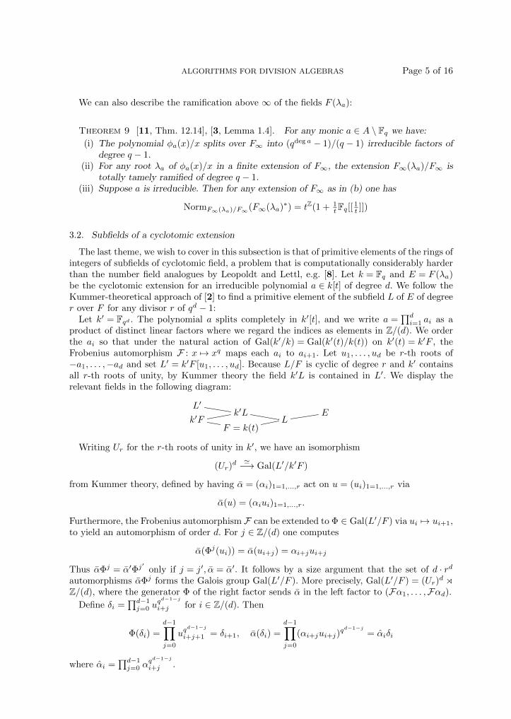
The last theme, we wish to cover in this subsection is that of primitive elements of the rings ofintegers of subfields of cyclotomic field, a problem that is computationally considerably harderthan the number field analogues by Leopoldt and Lettl, e.g. [8]. Let k = Fq and E = F (λa)be the cyclotomic extension for an irreducible polynomial a ∈ k[t] of degree d. We follow theKummer-theoretical approach of [2] to find a primitive element of the subfield L of E of degreer over F for any divisor r of qd − 1:

Let k′ = Fqd . The polynomial a splits completely in k′[t], and we write a =∏di=1 ai as a

product of distinct linear factors where we regard the indices as elements in Z/(d). We orderthe ai so that under the natural action of Gal(k′/k) = Gal(k′(t)/k(t)) on k′(t) = k′F , theFrobenius automorphism F : x 7→ xq maps each ai to ai+1. Let u1, . . . , ud be r-th roots of−a1, . . . ,−ad and set L′ = k′F [u1, . . . , ud]. Because L/F is cyclic of degree r and k′ containsall r-th roots of unity, by Kummer theory the field k′L is contained in L′. We display therelevant fields in the following diagram:

L′k′L E

k′F LF = k(t)

Writing Ur for the r-th roots of unity in k′, we have an isomorphism

(Ur)d '−→ Gal(L′/k′F )

from Kummer theory, defined by having α = (αi)1=1,...,r act on u = (ui)1=1,...,r via

α(u) = (αiui)1=1,...,r.

Furthermore, the Frobenius automorphism F can be extended to Φ ∈ Gal(L′/F ) via ui 7→ ui+1,to yield an automorphism of order d. For j ∈ Z/(d) one computes

α(Φj(ui)) = α(ui+j) = αi+jui+j

Thus αΦj = α′Φj′

only if j = j′, α = α′. It follows by a size argument that the set of d · rdautomorphisms αΦj forms the Galois group Gal(L′/F ). More precisely, Gal(L′/F ) = (Ur)

d oZ/(d), where the generator Φ of the right factor sends α in the left factor to (Fα1, . . . ,Fαd).

Define δi =∏d−1j=0 u

qd−1−j

i+j for i ∈ Z/(d). Then

Φ(δi) =

d−1∏j=0

uqd−1−j

i+j+1 = δi+1, α(δi) =

d−1∏j=0

(αi+jui+j)qd−1−j

= αiδi

where αi =∏d−1j=0 α

qd−1−j

i+j .


Setting vβ =∑d−1i=0 β

qiδi for β ∈ k′∗ we want to compute Gal(L′/F (vβ)). It follows fromαqi = αi+1 that

Φ(vβ) =

d−1∑i=0

Φ(βqi

δi) =

d−1∑i=0

βqi+1

δi+1 = vβ , α(vβ) =

d−1∑i=0

αiβqiδi =

d−1∑i=0

αqi

0 βqiδi = vα0β

An automorphism αΦ leaves F (vβ) fixed if and only if α0 = 1. Hence for such an αΦ, thefirst d− 1 components of α determine the last. This means that # Gal(L′/F (vβ)) = d · rd−1and

# Gal(F (vβ)/F ) = r

Lemma 10. One has F (vβ) = L.

Proof. We write ai = (t− βi) for suitable βi ∈ k′ with βqi = βi+1. Define u′1, . . . , u′d as qd −

1-st roots of −a1, . . . ,−ad. With E′ = k′F [u′1, . . . , u′d] we can analogously define Φ′, δ′i and v′β

and get Gal(E′/F ) = (k′∗)d o Z/(d). The restriction Gal(E′/F )→ Gal(L′/F ) is given by

(α0, . . . , αd−1)Φ′j 7−→ (αr′

0 , . . . , αr′

d−1)Φj , (3.2)

where r′ = (qd − 1)/r. We define α′ = (αr′

0 , . . . , αr′

d−1).A direct computation found in [2] reveals that φt(v

′β) = v′β

q+ Tv′β = v′β−1β

. Inductively thisgives φf (v′β) = v′f(β−1)β

. Therefore φh(v′β) = 0 and because the v′β are distinct, they have to be

exactly the h-torsion points of the Carlitz module. One concludes F (v′β) = E.As in the preceding construction we know that

Gal(E′/E) = {αΦj ∈ Gal(E′/F ) | α0 = 1}

Using the above restriction formula (3.2), we deduce from the previous paragraph

Gal(E′/F (vβ)) = {αΦj ∈ Gal(E′/F )) | α′0 = 1}

Obviously α0 = 1 implies α′0 = 1, so Gal(E′/E) ⊂ Gal(E′/F (vβ)) or equivalently E ⊃ F (vβ).From [L : F ] = [F (vβ) : F ] = r we find L = F (vβ).

Lemma 11. Keeping the above notation, the local Frobenius at an unramified prime g ∈ k[t]

of degree e, with g monic, is given by vβ 7→ vxβ where x =(g(βe−1)

)r′qd−e.

Proof. Split g into linear factors g = (t− b0) . . . (t− be−1) with bqi = bi+1. The Frobenius isgiven by taking the qe-th power modulo (g). One computes:

δqi = ar′

i δi+1, δqe

i = (ai+e−1aqi+e−2 . . . a

qe−1

i )r′δi+e

Reducing modulo g by substituting t 7→ b0 the base term can be simplified:

(ai+e−1aqi+e−2 . . . a

qe−1

i ) = (βi+e−1 − t)(βi+e−1 − tq) . . . (βi+e−1 − tqe−1

)

≡ (βi+e−1 − b0)(βi+e−1 − b1) . . . (βi+e−1 − be−1) (mod g)

= g(βi+e−1) = g(βe−1)qi

Finally we can compute:

vqe

β ≡d−1∑i=0

βqi+e

(g(βe−1))r′qiδi+e (mod g) =

d−1∑i=0

(β(g(βe−1))r′qd−e)q

i+e

δi+e = vxβ


Remark 12. Of course, there are other approaches to get a primitive element of L: In [1,Lemma 11] a normal integral basis of OE is given in terms of universal Gauss-Thakur sums.It can be combined with [2, Lemma 4], which states that taking the trace over L of a normalintegral basis yields an integral basis of OL. Alternatively the norm of a primitive h-torsionelement can be taken ([5, Theorem 4.3]).

These two alternative approaches need at least O(qd) multiplications in the big cyclotomicfield E as opposed to O(r) in the Kummer extension L′ as described above. Implementationsof all three constructions confirm the better performance of the approach introduced here.

4. The basic algorithm

Let S be a finite set of finite places of F , and for each v ∈ S, let sv = nv/rv be a reducedfraction, and define r = lcm(rv : v ∈ S). Then the theorem of Grunwald-Wang guarantees theexistence of a cyclic field L/F of degree r and of a cyclic algebra of the form D = (L/F, σ, a)whose local invariant satisfy invv(D) = sv.

For the simple algorithm below, we shall make the following further restriction:

Assumption 13. None of the rv is divisible by p, and ∞ /∈ S.

More concretely, the simple algorithm wishes to find a subextension L of E = F (λw) for aplace w of F , i.e., L/F is of prime conductor, such that

(1) r = [L : F ], and(2) for all v ∈ S we have rv|[Lv : Fv] =: dv.

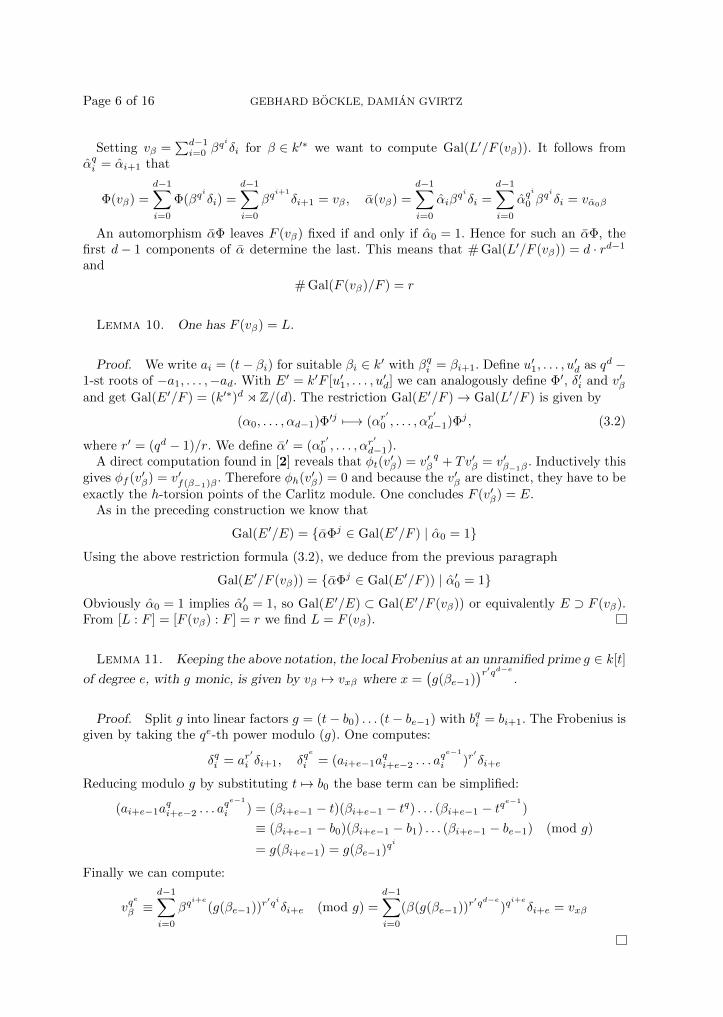
We fix a generator σ of G := Gal(E/F ) and denote by H ≤ G the subgroup correspondingto L. We display the situation in the following diagram

E

G=(A/hw)∗∼=Z/(qw−1)

H=〈σr〉

Ev

Gv∼=Z/(fv)

Hv=〈σdvv 〉

LG=〈σ〉∼=Z/(r)

LvGv=〈σv〉∼=Z/(dv)

F Fv,

where σv denotes the Frobenius endomorphism at v. A bar on top of an endomorphism is usedto denote the restriction of the endomorphism to the intermediate field L or Lv.

4.1. Global conditions

We define qw = qdeg(w). Then the global condition is r|qw − 1, i.e., that qdeg(w) ≡ 1 (mod r).Recall that we assume that p does not divide r here, so that q is a unit in Z/(r).

4.2. Local conditions

For the local degree of Ev/Fv (it depends on v and w, so we add both parameters into ournotation) we have

fv(w) = ord(A/w)∗(hv).

Hence the local decomposition group is

Gv = 〈σ(qw−1)/fv(w)〉 = 〈σv〉.

The decomposition group of Lv/Fv is now given by HGv/H. Since everything takes place insidethe cyclic group G the subgroup HGv is cyclic, and for the order dv of the quotient HGv/H


we deduce

dv = lcm(qw − 1

r, fv(w)

)/qw − 1

r= fv(w)/gcd

(qw − 1

r, fv(w)

).

The condition we require is rv|dv.

4.3. Statement of the algorithm

After a number of simple manipulations we obtain the following algorithm:

Algorithm 14. Input: an integer m ≥ 2, pairwise distinct irreducible elements h1, . . . , hmforming the set S, reduced fractions sv = nv/rv for v ∈ S. Output: a monic irreduciblepolynomial hw.

(i) Check whether∑v sv ≡ 0 mod Z. If not, stop procedure.

(ii) Check whether the hv are irreducible and pairwise distinct. If not, stop procedure.(iii) Divide each hv by its leading term, so that it is monic.(iv) Check whether the sv are reduced fractions – if not, reduce them.(v) Compute r = lcm(rv : v ∈ S). If p|r, then stop.(vi) Compute d0 = ord(Z/(r))∗(q).

(vii) Start for loop over j = 1, 2, 3, . . ..(viii) Start for loop over all monic irreducible polynomials hw of degree d0j.(ix) If h ∈ S, then go to next irreducible. If all irreducibles of degree d0j are tested, increase j.(x) Compute for v ∈ S the quantity fv(w) = ord(A/w)∗(hv) and check if it is divisible by

rv. If not go to next irreducible. If all irreducibles of degree d0j are tested, increase j.(xi) Check for v ∈ S whether gcd( qw−1r , fv(w)) divides fv(w)

rv. If test fails for one v, go to

next irreducible. If all irreducibles of degree d0j are tested, increase j.(xii) Return hw and end the loops.

While the algorithm provides a cyclotomic extension which is sufficient to construct a cyclicalgebra with the required invariants, the later explicit construction of a maximal Fq[t]-orderwill need to replace the condition rv|dv by the stronger condition of equality rv = dv. Thisamounts to changing the divisibility checks (xi) in the algorithm by tests for equality. Wewill refer to this altered algorithm as Algorithm 14 with strong conditions while the originalalgorithm will be referred to as Algorithm 14 with weak conditions.

4.4. Construction of L, σ and a

We now assume that the search for w was successful and set L = E〈σr〉, so that σ = σ|L is

a generator of Gal(L/F ).Then uv := r/dv is the smallest positive integer such that σuv ∈ Gv. In particular, both

σuv , and the Frobenius automorphism σv at v are generators of Gv ∼= Z/(dv). Therefore thefollowing definition makes sense:

Definition 15. Define u′v ∈ (Z/dvZ)∗, such that σuv = σu′vv .

This means that σuv acts on the residue field at v as α 7→ αqu′vv .

Let u′′v ∈ Z an inverse to u′v modulo dv. Then for a ∈ F we have

(L/F, σ, a)⊗F FvThm. 3

= (Lv/Fv, σu′vv , a)

Thm. 2(a)∼ (Lv/Fv, σv, au′′v ).


In particular

invv(L/F, σ, a) ≡ u′′vv(a)

dv(mod Z).

Locally at v we want to have invvD = nv/rv, i.e. nv/rv ≡ u′′v v(a)dv

(mod Z). Since dv is amultiple of rv, we obtain

nvdvrv≡ u′′vv(a) (mod dv).

Solving for v(a) yields

v(a) ≡ u′vnvdvrv

(mod dv). (4.1)

The above argument holds for all finite places. We define gv to be the integer such that

gv ≡ u′vnv (mod rv) and 0 ≤ gv ≤ rv − 1. (4.2)

We define a =∏v h

gvdv/rvv .

Theorem 16. With notation as above, D = (L/F, σ, a) is a central division algebra overF with invvD = sv for all places v of F .

Proof. The statement is clear for the invariants at all finite places different from w. Because∑sv = 0, it remains to show s∞ = 0. By Theorem 3, we have

(L/F, σ, a)⊗F F∞ = (L∞/F∞, σk, a),

where k > 0 is the smallest integer such that σk lies in Gal(L∞/F∞). But now observe that ais a norm from F∞(λw)∗ to F ∗∞ by definition of a∞ and Theorem 9(c), because t− deg aa is a1-unit in F∞ and hence a is a norm from F∞(λw)∗.

5. Termination of the algorithm

Theorem 17. Algorithm 14 terminates with weak and strong conditions.

We shall prove the theorem, by showing that the set of primes w for which the algorithmterminates is a Cebotarov set of positive density.

5.1. Weak conditions

We introduce a notation for the prime factorization of r, namely we denote it by r =∏i peii

for pairwise distinct prime numbers pi and integer exponents ei ≥ 1.The conditions on the sought for w are then as follows:(a) w /∈ S.(b) ordZ/(r)∗(q)|deg(w).(c) fv(w) := ordA/(w)∗(hv) is a multiple of rv, or in other words:

∀i : ordpi(rv) ≤ ordpi(fv(w)).

(d) ∀v ∈ S,∀pi: min(

ordpi(qw−1r

), ordpi(fv(w))

)≤ ordpi(fv(w))− ordpi(rv). This in turn

is equivalent to

∀v ∈ S,∀pi : if pi|rv then ordpi(qw − 1)− ordpi(r/rv) ≤ ordpi(fv(w)).


Lemma 18. Suppose condition (a) holds. Then condition (b) is equivalent to Frobw = 1 inGal(F (ζr)/F ) for ζr a primitive r-th root of unity.

Proof. Using that w should not ramify in F (ζr) and the Frobenius generates the localGalois group, one gets a chain of equivalences

Frobw = 1 ∈ Gal(F (ζr)w/Fw)⇔ [F (ζr)w : Fw] = 1⇔ [Fw(ζr) : Fw] = 1⇔ r|qw − 1,

where Fw denotes the residue class field of F at w.

Moreover under (d), condition (c) is superfluous, i.e., the join of the two becomes:

(e) ∀v ∈ S, ∀pi : if pi|rv then ordpi(qw − 1)− ordpi(r/rv) ≤ ordpi(fv(w)).

We define ei,v := ordpi(r/rv) + 1 whenever pi|rv, and note that under this condition we haveei,v ≤ ei since ordpi(rv) ≥ 1.

Lemma 19. Let Fw denote the residue field of F (ζr) at w and hv the reduction of hv in thatfield. Assuming that Frobw = 1 in Gal(F (ζr)/F ) and 0 ≤ ei,v ≤ ei, the following assertions areequivalent:

(i) Frobw = 1 in Gal(F (ζr,pei,vi

√hv)/F ),

(ii)pei,vi

√hv ∈ F∗w,

(iii) ordpi(fv(w)) ≤ ordpi(qw − 1)− ei,v .

Note that adjoining any pei,vi -th root of unity is a Kummer extension of F (ζr) since peii

divides r.

Proof. As in the proof of the previous lemma

Frobw = 1 ∈ Gal(F (ζr,pei,vi

√hv)/F )

⇔ Frobw = 1 ∈ Gal(F (ζr,pei,vi

√hv)/F (ζr))⇔

pei,vi

√hv ∈ F∗w

where the first equivalence uses that Frobw = 1 in Gal(F (ζr)/F ).

For (ii)⇒ (iii), let hv = xpei,vi ∈ F∗w. Then ordF∗w x|qw − 1, so

ordpi(fv(w)) = ordpi(ordF∗w(xpei,vi )) = ei,v + ordpi(ordF∗w x) ≤ ei,v + ordpi(qw − 1).

For (iii)⇒ (ii), let x be a generator of F∗w and xs = hv. Then because

ordpi(ordF∗w hv) = ordpi(fv(w)) ≤ ordpi(qw − 1)− ei,v

we know that ordpi(s) ≥ ei,v, hence pei,vi |s and

pei,vi

√hv is given by xs/p

ei,vi .

We deduce the following result, of which Theorem 17 with weak conditions is an immediatecorollary.

Proposition 20. The density of primes w in F satisfying (a)–(d) is

1

φ(r)·m∏j=1

∏i:pi|rvj

(1− 1

pei,vji

).


Proof. Define Ev :=∏i:pi|rv p

ei,vi for all v ∈ S and consider the tower of fields

F ′′ := F (ζr)(h1/Ev1v1 , . . . , h

1/Evmvm ) ⊃ F ′ := F (ζr) ⊃ F

Then (1) Gal(F ′/F ) = Z/φ(r)Z, (2) the extension F ′/F is unramified, (3) The extensions F ′j :=

F ′(h1/Evjvj )/F ′ are proper, linearly disjoint and ramified precisely at vj and totally ramified at

vj , (4) F ′′/F ′ is abelian with Galois group Gal(F ′′/F ′) ∼=∏mj=1 Z/EvjZ, (5) the extension

F ′′/F is Galois and its group is a semidirect product Gal(F ′′/F ′) o Gal(F ′/F ).To see properness in (3), note in the function field case that F ′/F is unramified but F ′j/F

ramifies at hvj ; because p is not allowed to divide rv, the extension F ′/F is Galois. Lineardisjointness follows because the extensions have distinct ramification places.

It follows that w is a place satisfying conditions (a)–(d) if and only if Frobw is trivial in

Gal(F ′/F ) and Frobw is non-trivial in all primary factors of Gal(F ′(h1/Evjvj )/F ′). From the

Cebotarov density theorem, e.g. [9, Sec. VII.13], we get the required density.

5.2. Strong conditions

We have to replace the first inequality in condition (d) with equality and call this (d’). Asabove we make (c) superfluous and set ei,v := ordpi(r/rv) + 1 for pi|rv. Using Lemma 19, werestate (d’).

(e’) If pi|rv, then

Frobw = 1 ∈ Gal(F (ζr,pei,v−1

i

√hv)/F ) ∧ Frobw 6= 1 ∈ Gal(F (ζr,

pei,vi

√hv)/F ).

(e”) If pi - rv, then Frobw = 1 ∈ Gal(F (ζr,peii

√hv)/F ).

The factors in Theorem 20 change to (pi − 1)/pei,vi for pi|rv and 1/peii for pi - rv. We deduce

the following result, of which Theorem 17 with strong conditions is an immediate corollary.

Proposition 21. The density of primes w in F satisfying the strong conditions is

1

φ(r)·m∏j=1

rvjr

∏i:pi|rvj

(1− 1

pi

).

6. Constructing a maximal Fq[t]-order

The present section describes how to obtain a maximal order for D = (L/F, σ, a) constructedby the algorithm with strong conditions, i.e., in the case where rv = dv for all v ∈ S; in thissection σ denotes a generator of Gal(L/F ), e.g. the σ from Subsection 4.4, and by order wewill always mean Fq[t]-order.

First, observe that we are dealing with a local question:

Theorem 22 [10, 11.6]. An order Λ is maximal if and only if for all places v 6=∞ of Fthe completion Λv is maximal in Dv.

We are going to describe how to maximize the order Λ = ⊕r−1i=0OLτ i at the different placesof F . The globally maximal order is the linear hull of all the locally maximized orders.


6.1. The discriminant of a maximal order

An important tool to decide whether an order is maximal inside a central simple algebra isits discriminant. Here we collect the relevant facts needed for the construction of a maximalorder in D starting with Λ =

⊕r−1i=0 OLτ i.

The following result is immediate from [10, Thm. 32.1]:

Proposition 23. Suppose D has local invariants svrv

at the finite set of places S of K withcorresponding primes hv and set r = lcm(rv : v ∈ S). Then for a maximal order Λ of D one

has disc(Λ) =(∏

v∈S hr− r

rvv

)r.

Corollary 24. Let D be as in Theorem 16 and let Λ be the order ⊕r−1i=0OLτ i. Then(i) The order Λ is maximal at all places outside S ∪ {w}.

(ii) The discriminant of Λ at w is disc(L/K)r = pr(r−1) or disc(L/K)r = hr(r−1)w .

(iii) The discriminant of Λ is hr(r−1)·gvdv/rvv at v ∈ S.

(iv) The order Λ is maximal at v ∈ S if and only if rv = dv = r and gv = 1.

Proof. The first three parts are immediate from the computation of disc(Λ) in Corollary 7and the standard formula for discriminants of abelian extensions of Fq(t) in terms of conductorsof the defining characters; see [12].

For the last part we need to compare (iii) with the formula in Proposition 23. This gives the

condition hgvdv/rv·r(r−1)v

!=(hr− r

rvv

)r. It is equivalent to gv

dvrv

(1− 1r ) = 1− 1

rv. From this (iv)

is immediate.

6.2. The ramified place w

L/F is totally ramified at w and we can write Dw = (Lw/Fw, σ, a), where σ par abus denotation denotes the unique extension of σ onto Lw. Because invwD = 0 we know that anisomorphism Dw

∼= Mr(Fw) exists. Moreover this isomorphism can be described explicitly intwo steps:

Theorem 25 [10, Proof of Thm. 30.4].(i) There exists an element f ∈ O∗Lw such that NormLw/Fw f = a. It induces an iso-

morphism (Lw/Fw, σ, 1)→ (Lw/Fw, σ, a) by letting Lw fixed and τ 7→ (fτ). In fact,the existence of a solution to the norm equation is equivalent to (Lw/Fw, σ, 1) ∼=(Lw/Fw, σ, a).

(ii) An isomorphism (Lw/Fw, σ, 1)→ EndFw(Lw) ∼= Mr(Fw) is given by τ 7→ σ, x 7→ xLwfor x ∈ Lw, where xLw denotes multiplication by x. After choosing a basis e =(e1, . . . , er) of OLw over Ow, and writing xLwe = eTx, σe = eP for unique matrices Tx, Pin Mr(Fw), the isomorphism (Lw/Fw, σ, 1)→Mr(Fw) is given by τ 7→ P , x 7→ Tx.

In general, Mr(Fw) has many maximal orders, namely Mr(Ow) and all its conjugates ([10,17.3]). Luckily, under the above isomorphism we have Λw ⊂Mr(Ow). To see this, first note Λwremains unchanged under the first isomorphism as f ∈ O∗Lw . Under the second isomorphismthe action of Λw on Lw lies in the stabilizer of OLw which is equal to Mr(Ow) with the choiceof an integral basis.

6.2.1. Solving the norm equation Now we describe how to find the solution f of thenorm equation by a limit procedure: Choose a uniformizer π at w, so that p = OLwπ is the


maximal ideal of OLw . The unit group ULw = OLw − pw has the filtration U0Lw

= ULw , U iLw =

1 + pi, i ≥ 1. We recall that U0Lw/U1

Lw∼= F∗w and U iLw/U

i+1Lw∼= piw/p

i+1w∼= Fw, where the second

isomorphism depends on π. The same definitions can be made for Fw.The higher ramification groups Gi of Gw = Gal(Lw/Fw) form a decreasing sequence of

normal subgroups for i ≥ −1. As proven in [13, Cor. IV.2.2,3] the higher quotients Gi/Gi+1

vanish for p - r (being direct products of groups of order p). Thus Gw = G0, Gi = 1, i ≥ 1 andwith ψ(n) = rn we get

Theorem 26 [13, Prop. V.6.8, Cor. V.6.2].

(i) For every integer n ≥ 0 one has

N(Uψ(n)Lw

) ⊂ UnKw , N(Uψ(n)+1Lw

) ⊂ Un+1Kw

,

where N = NormLw/Fw . By passing to the quotients this yields

N0 : F∗w → F∗w, Nn : Fw → Fw for n ≥ 1.

(ii) The map N0 is given by ξ 7→ ξr.(iii) The map Nn is surjective and given by ξ 7→ βnξ for some βn ∈ F∗w.

Using this description of the norm (βn can be determined experimentally) we can constructfn =

∑nk=0 akπ

rk that approximate a solution f up to order rn for all n ≥ 0.

6.2.2. Necessary precision Let Λ′w be the maximal order Mr(Ow), so that Λw ⊂ Λ′w. Sinceboth are finitely generated Ow modules of the same rank, there exists an integer s ≥ 0 suchthat πsΛ′w ⊂ Λw.

In terms of bases (e′1, . . . , e′r2) and (e1, . . . , er2) of Λ′w and Λw we write e′i = π−s

(∑j αijej

)for suitable αij ∈ Ow. Now suppose aij ≡ aij (mod πs): Then defining e′i := π−s

(∑j αijej

),

a set of generators of Λ′w is given by{e′1, . . . , e′r2 , e1, . . . , er2}. One concludes that it is enoughto solve the norm equation up to order s− 1.

Theorem 27. The integer s can be chosen as r.

Proof. Consider the r × r-Vandermonde matrix with columns (πi, σ(πi), . . . , σr−1(πi))t

for i = 0, . . . , r − 1. Acting from the right on (λ1, . . . , λr) ∈ F rw it gives the image of(π0, π1, . . . , πr−1) under

∑i λiτ

i. The condition Λ′w ⊂ π−rΛw is equivalent to showing thatall∑i λiτ

i which send (π0, π1, . . . , πr−1) to OrLw lie in π−rΛw, i.e., the inverse V −1 sends OLwto π−rOLw .

Thus, we only need to know the denominators of the inverse of a Vandermonde matrix.According to [7, Exerc. 40], they are given by σi(π)

∏1≤k≤r,k 6=i(σ

i(π)− σk(π)). Because ofG0 = Gw, G1 = 1 all factors have valuation 1 and the total valuation is r.

Lemma 28. It suffices to solve the norm equation up to order 0.

Proof. Recall that the solution f was constructed in order jumps of size r.

6.2.3. Fixing the denominator The approximated generators e′1, . . . , e′r2 may have denom-

inators at places different from w. To make sure that we still have a multiplicatively closed


order, multiply the generators with the prime-to-w part, so that the order Λ′′ they generatestill equals Λ′w at w but is contained in the original order Λv at all v 6= w.

Because this inclusion in Λv may be proper, the global order sought-after (which is maximalat w but Λv at other places v) is the linear hull of Λ′′ and Λ.

6.3. Unramified places v ∈ S

For convenience, fix the notation d := dv, u := r/d throughout this section and assume d =rv (strong conditions). Fix prolongations w0, . . . , wu−1 of v to L s.t. σ acts on the wi’s bysending each to the next one and wu−1 to w0. In other words σ sends each component ofM := L⊗ Fv =

⊕u−1i=0 Li to the next one, where Li := Lwi . We construct an order maximal at

v containing Λ = ⊕r−1i=0OLτ i.Locally, D is given as:

D ⊗ Fv = M [τ ]/(τ r − a) =

(u−1⊕i=0

Li

)[τ ]/(τ r − a) =

u−1⊕i,j=0

(Li[τ

u]/((τu)d − a))τ j

Defining Di := Li[τu]/((τu)d − a), one knows that Di

∼= Dj for all 0 ≤ i, j ≤ u− 1 and M ∼=Mu(D0) (especially the Di have the same local invariant). Multiplication of elements in theright hand side of the above equation works via

σ : Di → Di+1, b(τu)s 7→ σ(b)(τu)s, αβ =

{0 i 6= j

α ·Di β i = j(6.1)

for b ∈ Li, α ∈ Di, β ∈ Dj .For d = rv (strong conditions) the algebra Dj actually is a skewfield, cf. [10, 31.6].

Theorem 29 [10, 13.3]. Let x ∈ Dj have valuation 1/d. Then Λ′v = ⊕d−1i=0OLjxi is amaximal order in Dj .

Now v(τu) = v((τu)d)/d = v(a)/d, hence for a uniformizer h of v in Fv

v(hm(τu)n) = m+ nv(a)/d.

Since (v(a), d) = 1 the extended Euclidean algorithm yields m,n ∈ Z with md+ nv(a) = 1 andhm(τu)n is the required element. Hence, in Dj we get the maximal order:

ODj := OLj [hm(τu)n].

Next, we will give an explicit description of a maximal order in (M/Fv, σ, a) as stabilizer ofa suitable lattice.

Lemma 30. V :=⊕u−1

i=0 Diτi is a left (M/Fv, σ, a)-submodule of (M/Fv, σ, a).

Proof. V is obviously closed under addition. It remains to show that left multiplicationwith “scalars” sends V to V . So let

a =

u−1∑i,j=0

αiτj ∈ (M/Fv, σ, a), x =

u−1∑i=0

βiτi ∈ V

Then a straightforward calculation shows

a · x =

u−1∑i,j=0

αiτju−1∑k=0

βkτk =

u−1∑i,j,k=0

αiσj(βk)τ j+k

(6.1)=

u−1∑i,j,k=0,j+k=i

αiσj(βk)τ i ∈ V


We now define a maximal lattice in V by ΛV :=⊕u−1

i=0 ODiτ i.Furthermore define three lattices in M [τ ]/(τ r − a):

R0 :=

u−1⊕i=0

i⊕j=i−u+1

ODiτ j ⊆ R1 :=

u−1⊕i=0

u−1⊕j=0

ODiτ j ⊆ R2 :=

u−1⊕i=0

u−1⊕j=0

OLi [τu]τ j

Note that R1 is the v-adic closure of OL[τ, hm(τu)n] and R2 the v-adic closure of OL[τ ].

Theorem 31. R0 equals the stabilizer of ΛV (and is therefore a maximal order).

Proof. Let i, k run from 0 to u− 1 and j from i− u+ 1 to i. Note first that ODiτ jODkτk =ODiσj(ODk)τ j+k = ODiODj+kτ j+k. By (6.1) the last term is non-zero only if i = j + k, inwhich case it lies in ΛV . This proves ‘⊆’. We now show the converse inclusion ‘⊇’:

Let α =∑i,j αijτ

j with αij ∈ Di for all i = 0, . . . , u− 1. If α lies in the stabilizer, then it

maps test elements x = βkτk with βk ∈ ODk to ΛV :

αx =∑i

αi,i−kσi−k(βk)τ i

!∈ ΛV

From this we deduce that αi,i−k ∈ ODi for all k = 0, . . . , u− 1. Therefore α ∈ R0.

The explicit description of the maximal order R0 can be lifted to that of a global ordermaximal at v. Before stating this result, we need a short lemma:

Lemma 32. Choose integers et for t = 0, . . . , u− 1 such that

ODi = OLi [hm(τu)n] =

d−1⊕t=0

OLihet(τu)t.

Furthermore set ed := −v(a), so that ODi =⊕d

t=1OLihet(τu)t.Then et−1 − et ∈ {0, 1} for all 0 < t ≤ d.

Proof. het(τu)t has valuation between 0 and 1− 1/d, so

1 > |v(het−1(τu)t−1)− v(het(τu)t)| = |et−1 − et − v(τu)|

Noting that 0 ≤ v(τu) = v(a)/d(4.2)= (gid/ri)/d = gi/ri < 1, the claim follows.

We now rewrite the maximal order R0:

R0 =

u−1⊕i=0

i⊕j=i−u+1

d−1⊕s=0

OLihes(τu)sτ j = R1 +

u−1⊕i=0

u−1⊕j=i+1

d−1⊕s=0

OLihes(τu)sτ j−u

= R1 +

u−1⊕i=0

u−1⊕j=i+1

d−1⊕s=0

OLihes(τu)s−1τ j = R1 +

u−1⊕i=0

u−1⊕j=i+1

d−1⊕s=0

OLihes+1(τu)sτ j

Let (bij)j=0,...,d−1 be a basis of ki/k (the residue field of Li over that of Fv) for all i =0, . . . , u− 1. Choose lifts bij to OLi and bij to OL. Note that OL/(h) = ⊕iOLi/(h), so that bij

of 16 ALGORITHMS FOR DIVISION ALGEBRAS

can be thought of as a first order approximations of the tuple (0, . . . , 0, bij , 0, . . . , 0). Then

R0 = R1 +

u−1∑i=0

u−1∑j=i+1

d−1∑s=0

d−1∑t=0

Av bithes+1(τu)sτ j = R1 +

u−1∑i=0

u−1∑j=i+1

d−1∑s=0

d−1∑t=0

Avbithes+1(τu)sτ j .

The last equation follows because

Av(bit − bit)hes+1(τu)sτ j ⊂⊕OLihes+1+1(τu)sτ j

Lem. 32⊂

⊕OLihes(τu)sτ j ⊂ R1.

The above formula for R0 provides a global lift of R0. It is the order

OL[τ, hm(τu)n] +

u−1∑i=0

u−1∑j=i+1

d−1∑s=0

d−1∑t=0

Abithes+1(τu)sτ j .

Fixing the denominator at other places is not necessary.

6.4. Unramified places v /∈ S

For these places, any order containing Λ = OL[τ ] will be maximal since the discriminantcommutes with localization and disc(Λ) = ad(d−1) disc(L/K) is a local unit.

References

1. Bruno Angles and Federico Pellarin. Universal gauss-thakur sums and l-series. arXiv:1301.3608, 2013.2. R. J. Chapman. Carlitz modules and normal integral bases. J. London Math. Soc. (2), 44(2):250–260,

1991.3. Steven Galovich and Michael Rosen. Units and class groups in cyclotomic function fields. J. Number

Theory, 14(2):156–184, 1982.4. David Goss. Basic structures of function field arithmetic. Ergebnisse der Mathematik und ihrer

Grenzgebiete (3), vol. 35. Springer-Verlag, Berlin, 1996.5. Venkatesan Guruswami. Cyclotomic function fields, artin-frobenius automorphisms, and list error

correction with optimal rate. Algebra & Number Theory, 4(4):433–463, 2010.6. Jens Carsten Jantzen and Joachim Schwermer. Algebra. Springer, first edition, 2006.7. Donald E. Knuth. The art of computer programming. Vol. 1. Addison-Wesley, Reading, MA, 1997.

Fundamental algorithms, Third edition.8. Gunter Lettl. The ring of integers of an abelian number field. Journal fur die reine und angewandte

Mathematik, 404:162–170, 1990.9. Jurgen Neukirch. Algebraische Zahlentheorie. Springer, first edition, 1992.

10. Irving Reiner. Maximal Orders. Academic Press Inc. (London) Ltd., 1975.11. Michael Rosen. Number theory in function fields. Graduate Texts in Mathematics, vol. 210. Springer-

Verlag, New York, 2002.12. Martha Rzedowski-Calderon and Gabriel Villa-Salvador. Conductor-discriminant formula for global

function fields. Int. J. Algebra, 5(29-32):1557–1565, 2011.13. Jean-Pierre Serre. Local fields, volume 67 of Graduate Texts in Mathematics. Springer-Verlag, New York,

1979. Translated from the French by Marvin Jay Greenberg.

Gebhard BockleUniversitat HeidelbergInterdisziplinares Zentrum fur

wissenschaftliches Rechnen (IWR)Im Neuenheimer Feld 36869120 HeidelbergGermany

[email protected]

Damian GvirtzThe London School of Geometry and

Number TheoryDepartment of MathematicsUniversity College LondonGower StreetLONDONWC1E 6BTUnited Kingdom

[email protected]

division algebras and maximal orders for given invariants · division algebras and maximal orders...

Documents