divorce, abortion and children’s sex ratio: the …ftp.iza.org/dp8230.pdf · divorce, abortion...
TRANSCRIPT
DI
SC
US
SI
ON
P
AP
ER
S
ER
IE
S
Forschungsinstitut zur Zukunft der ArbeitInstitute for the Study of Labor
Divorce, Abortion and Children’s Sex Ratio:The Impact of Divorce Reform in China
IZA DP No. 8230
May 2014
Ang SunYaohui Zhao
Divorce, Abortion and Children’s Sex Ratio:
The Impact of Divorce Reform in China
Ang Sun Renmin University of China
Yaohui Zhao Peking University
and IZA
Discussion Paper No. 8230 May 2014
IZA
P.O. Box 7240 53072 Bonn
Germany
Phone: +49-228-3894-0 Fax: +49-228-3894-180
E-mail: [email protected]
Any opinions expressed here are those of the author(s) and not those of IZA. Research published in this series may include views on policy, but the institute itself takes no institutional policy positions. The IZA research network is committed to the IZA Guiding Principles of Research Integrity. The Institute for the Study of Labor (IZA) in Bonn is a local and virtual international research center and a place of communication between science, politics and business. IZA is an independent nonprofit organization supported by Deutsche Post Foundation. The center is associated with the University of Bonn and offers a stimulating research environment through its international network, workshops and conferences, data service, project support, research visits and doctoral program. IZA engages in (i) original and internationally competitive research in all fields of labor economics, (ii) development of policy concepts, and (iii) dissemination of research results and concepts to the interested public. IZA Discussion Papers often represent preliminary work and are circulated to encourage discussion. Citation of such a paper should account for its provisional character. A revised version may be available directly from the author.

IZA Discussion Paper No. 8230 May 2014
ABSTRACT
Divorce, Abortion and Children’s Sex Ratio: The Impact of Divorce Reform in China*
This paper explores how the relative circumstances of men and women following marital dissolution affect sex-selection behavior within marriages. China’s 2001 divorce reform liberalized divorce in favor of women and secured women’s property rights after separation. We use this improvement in women’s bargaining power in marriage for a regression discontinuity analysis of the demand for sex-selective abortions. We show that the increase in women’s bargaining power reduces the propensity to have a son after a firstborn daughter by 8.9 percentage points. We also find that the effect is larger for women with higher health risks. JEL Classification: D13, J12, J13, J16 Keywords: gender inequality, intra-household allocation, divorce law Corresponding author: Yaohui Zhao China Center for Economic Research Peking University Beijing 100871 P. R. China E-mail: [email protected]
* The authors thank Andrew Foster, Anna Aizer, Vernon Henderson, Sriniketh Nagavarapu, Nancy Qian, and Anja Sautmann for very helpful suggestions on earlier versions of this paper. We also thank participants at the Applied Micro Lunch, Race and Inequality workshop at Brown University, NEUDC 2010, RES 2011 and CESI 2012 for useful comments. All mistakes are our own.
1 Introduction
Household outcomes depend on decisions made by spouses who may often dis-
agree. In these circumstances, the distribution of decision-making power may
matter a great deal for intra-household allocation outcomes. Among these
outcomes, gender inequality in the next generation of households is a topic
of much interest among social scientists and policy makers. The most salient
manifestation of persistent gender inequality is the phenomenon of "missing
women" (Sen, 1990; 1992). This phenomenon refers to the smaller number of
women than would be expected in the population if girls and women through-
out the developing world were born and died at the same rate as boys and
men. Today, among the estimated six million missing women, 23 percent were
never born (Du�o, 2012). In this paper, we exploit China�s 2001 divorce re-
form to investigate the e¤ect of women�s bargaining power within a household
on sex-selective abortions and suggest a mechanism to explain our �ndings.
Besides "missing girls", a large and growing literature in economics has
associated improvements in women�s bargaining power with decreased disad-
vantages among daughters, in such dimensions as schooling, health and health
care.1 Because some earlier work has su¤ered from problems of endogeneity
(see Du�o (2003) for a detailed review), more-recent studies have examined
the impact of certain exogenous shocks to women�s income on children�s well-
being.2However, these shocks increased both women�s bargaining power and
the relative return to having daughters (Qian, 2008) or the household�s total
income (Du�o, 2003). When children are regarded as household investment
or consumption (Banerjee, 2004), the shocks to women�s economic value can-
not be used to rule out the unitary model of household decision making or to
identify the e¤ect of bargaining power on daughters�well-being.
A �cleaner� shock on bargaining power can be one that changes �extra
1Previous research shows that when women have more control over household income,the mortality rate for daughters decreases. For example, see Ben Porath (1967, 1973, 1976);Burgess and Zhuang (2000); Clark (2000); Du�o (2003); Das Gupta (1987); Foster andRosenzweig (2001); Rholf, Reed and Yamada (2010); Rosenzweig and Schultz (1982); andThomas, Strauss and Henriques (1991), to cite just a few.
2For example, Du�o (2003) uses the pension windfall for grandmothers in South Africa;Qian (2008) uses the increase in the tea price in China.
2
household environmental parameters�(EEP) or �distribution factors�(Brown-
ing and Chiappori,1998). Because such a shock in�uences the decision-making
process but not the budget constraint (or preferences), the resulting change
in intra-household resource allocation points directly to diverging preferences
between men and women. Legal innovations in the area of property division
upon divorce satisfy such identi�cation conditions because they a¤ect the re-
lative status at the "threat-point" or the "exit" of the marriage (Mansor and
Brown, 1980; McElroy and Horney, 1981; McElroy, 1990) without changing
household budget constraint. A large literature has provided empirical evid-
ence that laws governing the division of property upon divorce have signi�cant
impacts on women�s bargaining power in the household.3But this literature has
not yet investigated the outcome of gender disparity among children in house-
holds.
China�s 2001 divorce reform liberalized divorces in favor of women and se-
cured women�s property rights after separation. By improving women�s outside
option (welfare level in the event of relationship dissolution), the amendment
e¤ectively strengthened their status within their partnerships. Using this di-
vorce reform for a regression discontinuity analysis on sex-selective abortion
demand, we provide a rigorous identi�cation of the impact of intra-household
bargaining power on sex-selective abortions against girls.
Our main empirical analysis uses data from China�s 2005 One-Percent Pop-
ulation Survey. We focus on the sex ratio of the second children following
�rstborn girls, because according to the prior literature, this is the margin
at which sex-selective abortions are heavily used. We detect a discontinuous
decline in the sex ratio (de�ned as the ratio of the number of boys to the
number of girls) among the cohort conceived in February 2002, shortly after
the de facto implementation of China�s amended divorce law on December 26,
2001. During the brief period around the detected timing threshold of Febru-
ary 2002, the propensity to have a son after a �rstborn daughter decreased by
3Prior empirical research has studied the impact of divorce law changes in countries suchas the U.S., Canada and Brazil on such household outcomes as labor supply (Gray, 1998;Stevenson, 2008; Rangel, 2006; LaFortune et al., 2012); household specialization (Stevenson,2008); domestic violence (Aizer, 2011; Stevenson and Wolfers, 2006); and children�s well-being (Gruber 2004; Rangel 2006).
3
8.9 percentage points. Our results are robust to standard regression discon-
tinuity checks. We also review all policies that could potentially impact the
incidence of sex-selective abortions in the relevant time window and rule them
out as the primary driving force behind the decline in children�s sex ratio.
We o¤er supplementary evidence on the increase in children�s caloric intake
and the decrease in husbands� cigarette and liquor consumption, which are
widely regarded in the literature as evidence of an improvement in women�s
bargaining power.
To interpret the e¤ect of women�s bargaining power on less missing girls, the
previous literature implicitly assumes women�s lesser prejudice against daugh-
ters.4 However, in countries with highly skewed sex ratios, such as China and
India, it is plausible to cast skepticism on this assumption (Anold, Choe and
Roy, 1998; Chu, 2001). Women�s son preference may even be stronger be-
cause a son will bring them more respects from the husbands and in-laws as
well as instrumental supports in their old age. While we do not aim to reject
di¤erential values attached to sons, in this paper we suggest a novel mech-
anism based on the observation of asymmetric health-related costs between
the wife and husband upon sex-selective abortions. This distinction is mean-
ingful because the implications from the model can be applied to other cases
of household public-good provision, including those in which there is no clear
gender di¤erence in preferences.
We draw on the insights of non-transferable utility (Chiappori, Lyigun and
Weiss, 2007) to demonstrate how these asymmetric costs can a¤ect demand
for sex-selective abortions. Speci�cally, bearing the lion�s share of physical
and psychological health-related costs of sex-selective abortions, the wife will
demand compensation in terms of private consumption and the husband will
face the tradeo¤ between sacri�cing his private consumption and attaining a
desirable sex composition of children. The amount of compensation upon abor-
tion is determined by women�s bargaining position. When the divorce reform
4The theoretical foundation can by formalized by the collective model laid out by Blun-dell, Chiappori and Meghir (2005), which focuses on the context of sharing one publicgood when one member�s marginal willingness to pay is more income-sensitive; then, animprovement in this member�s control of the family income will increase this public goodexpenditure.
4
increased women�s bargaining power, the husband found it more �expensive�
to make his wife accept sex-selective abortion and households on the margin
will switch from abortion to non-abortion. We show that under nontrans-
ferability, the utility Pareto frontiers of abortion and non-abortion intersect,
and the improvement in women�s divorce options will reduce the wife�s health-
damaging e¤orts toward public-good provision (i.e., sex-selective abortion in
our context).
Note that the health-related costs on sex-selective abortions are higher for
women of low fecundity or being pregnant in late age. Therefore, we use
the gap between marriage and having the �rst child5 as a proxy for women�s
health-related costs on sex-selective abortion during the second pregnancy
after controlling women�s age at marriage, schooling years and SES. These
characteristics could capture the opportunity costs of having children and the
initial bargaining power prior to the reform. We �nd that after the amended
divorce law, a one-year delay in having the �rstborn daughter results in an
extra 2.6-percentage-point reduction in the probability of having a second-
born son.
The paper is organized as follows: In Section 2, we describe the background
of China�s widespread sex-selective abortions and the 2001 divorce reform. In
Section 3, we present the theoretical model and derive the predictions on the
less-skewed sex ratio caused by the divorce reform and larger e¤ect of the re-
form among women with higher health-related costs. In Section 4, we establish
the causal link between divorce reform and the decline in children�s sex ratio
and present the RD estimands. In Section 5, we explore the heterogeneity in
the magnitude of the e¤ect across women with di¤erent health-related costs
to shed light on the mechanism of the e¤ect. In Section 6, we conduct robust-
ness checks and provide supplementary evidence. Finally, Section 7 presents
concluding remarks.
5Sturm and Zhang (1993) use �rst conception interval as a measure of fecundibility.
5
2 Sex-Selective abortions and Divorce in China
2.1 Sex-Selective Abortions
Under the restrictive family-planning policy in China, induced abortion fol-
lowing ultrasound B sex screening is the most common form of sex selection
(Ebenstein, 2008; Li, 2007; Li, Wei and Feldman, 2005;Zeng, 1993). The
stipulations also prevent individuals from using divorce to evade the family-
planning policy: remarried couples qualify to have a child of their own only
when one party does not already have a child and the other does not have
more than one. 6
In rural areas, six provinces apply the restrictive one-child rule and a signi-
�cant amount of �ne will be charged for a second birth (Scharping, 2003); �ve
provinces generally allow two births; and 19 other provinces apply the "Girl
Exception" or the so-called "1-Son-2-Children" policy, meaning that if the
�rstborn is a daughter, a couple can have another child. But a couple is gen-
erally not allowed to have more than two children. Sex-selective abortions are
seldom used for the �rst birth but heavily used for the second pregnancy after
a �rstborn daughter (Ebenstein, 2008; Li, 2007; Li, Wei and Feldman, 2005;
Li, 2007). Therefore, in this paper, we focus on the sex of the second-born
child after having a �rstborn daughter.
Sex-selective abortions inevitably harm women�s physical and, especially,
psychological health. The sex of a fetus is usually detected during the second
trimester or later. An abortion in that period, in comparison to a �rst-
trimester abortion, requires higher doses of the drug Misoprostol to induce
labor; in addition, the surgery takes longer, and there are more side e¤ects. In
the 1997 Survey of Population and Reproductive Health in China, 75.46 per-
cent of women stated that abortion had a negative impact on their physical
and psychological health, with 18.58 percent rating the impact as major.
6The restriction was relaxed somewhat in a few provinces after our study period, since2008.
6
2.2 Divorce: The Status Quo and the New Divorce Law
In rural China, the divorce rate, on average, is traditionally low (Zeng and Wu,
2000). In our 0.1- percent sample from the 2000 Population Census and the
25-percent sample from the 2005 One-Percent Population Survey, there were
only 3.62 and 3.78 divorces per 100 marriages among women between ages
25 and 35 in 2000 and 2005, respectively.7The divorce rate is higher among
younger couples and in cities.
The main reason for the low divorce rate in rural areas is that women
have poor divorce options. The village generally supplies land and homestead
through the husband�s family, and women forfeit these properties upon di-
vorce. Parents treat a married daughter as "water poured out" and, thus,
usually do not welcome her back. In a case study by Chan and Liu (2000), the
researchers record that women who would like to divorce but endure their un-
happy marriages assume that, were they to leave their marriages, they would
face an immediate loss of housing and �nances.
The amended divorce law was announced on April 28, 2001, and the judi-
cial interpretation of the amendment, which serves as an operational guideline
for implementing the reform, was issued on December 26, 2001. The new di-
vorce law speci�ed property division in greater details, speci�cally restating
rural women�s rights to land and housing upon divorce. Women�s property
rights had been announced before this amendment, but this reform added new
articles to improve enforcement.8 Moreover, the guidelines for implementa-
tion made it clear that if after divorce, the wife were unable to maintain a
basic standard of living according to the properties entitled upon divorce, the
husband would be responsible for compensating her to that standard. In par-
ticular, the wife would be regarded as not meeting the "basic living standard"
if she did not have a place to live.
7In both datasets, marital status is reported with the following choices: married, remar-ried, divorced, widowed and never married. We de�ne divorce as including remarriages.Because we restrict the sample to ages 25-35, remarriage after widowhood is rare in thedata.
8Article 47: "During the divorce proceedings, if one party attempts to conceal, transfer,sell or destroy community property, or falsify liability with the intention of misappropriatingthe other party�s property, when property is partitioned in court, the court may award tothe party at fault either a smaller amount of property or none at all."
7
Another important amendment of this divorce law is that it makes uni-
lateral divorce possible in the case of domestic violence and extra-marital re-
lationships, which are grounds used mainly by women. The new law also
stipulates that when a divorce is granted, the innocent party can now seek
damages from the guilty party.9
3 The Model
3.1 Basic Setup
To better understand the interplay between children�s sex ratio and women�s
divorce options, we consider a simple theoretical framework with public-good
provision in the household.10We assume that both spouses place the same
value, �, on the public good, the sex composition of children. We focus on
households that are about to have a second child, given that the �rst is a girl.
Assume that a �rstborn daughter brings utility �. For simplicity, assume that
a second daughter does not improve the spouses�utility. is the utility level
of having a second-born son. Therefore, � 2 f�; g. > �, indicates the
preference for sons. We denote the husband�s utility within marriage by u and
the wife�s utility within marriage by v:
u = xH + �
v =xWe+ �
where xH and xW are the private consumption of the husband and wife, re-
spectively. e is the e¤ort that the wife extends to increase the chance of having
a son, e 2 feA; eNAjeA > eNA > 1g. eNA and eA represent e¤orts without andwith sex-selective abortion, respectively. Assuming that the natural probab-
ility of having a son is 0.5 in each pregnancy, E� = 0:75 + 0:25� if e = eA,
9For stipulations on damage compensation for domestic violence, see Article 46 (3) and(4), and for the damage compensation for bigamy and extra-marital relationships, see Article46 (1).10We assume away unwanted pregnancies and ine¢ ciencies generated by frictions or asym-
metric information between the spouses.
8
while E� = 0:5 + 0:5� if e = eNA:
Note that the utility within marriage is not transferable between the spouses.
Speci�cally, the e¤ort e to provide public good will change the marginal rate
of substitution between the husband�s and the wife�s private consumption, im-
plying di¤erent slopes for the linear utility Pareto frontiers upon abortion and
non-abortion. The speci�c utility function can be generalized to any utility
that satis�es @@e
�@v@xW
�< 0 and @
@e
�@v@xH
�= 0, where the e¤ort level e exerted
by the wife depreciates her marginal utility of private consumption while the
husband�s remains intact or less a¤ected. 11
We assume that the husband makes decisions about sex-selective abortion
and consumption division, and the wife can reject his arrangements.12 If she
rejects them, divorce will be granted, and she will receive her reservation util-
ity, vd � cW . The cost of divorce for spouse i is ci, i = fH;Wg, which isdetermined by the legal environment or the so-called "extra-household envir-
onmental parameters" (Browning and Chiappori, 1998). In the case of this
article, ci re�ects the disutility from forfeiting entitled property and the costs
of going through legal procedures to get divorced. vd describes the best divorce
options for the wife, which are determined by her intrinsic characteristics (such
as personality and looks) and follow a distribution with density f (vd). The
wife rejects her husband�s choice if v < vd � cW . The e¤ect of the divorce lawis formalized as decreasing in cW .13
11The assumption on utility can be further relaxed to satisfy the condition @@e
�@v@xW
�<
@@e
�@v@xH
�:
12The assumption does not contradict the patriarchal tradition in rural China. In addition,the intuition of the model applies to other methods of surplus division that set up a monotonepositive relationship between the wife�s utility within marriage and upon divorce.13More generally, when the wife rejects the arrangements, divorce is granted with probab-
ility �. When divorce cannot be attained, the wife�s within-marriage utility could be lowerthan her reservation utility upon divorce. The husband will satisfy the wife to the level ofutility upon divorce only if � and cH are large enough. The amended divorce law couldalso cause an increase in � to make divorce a more relevant �threat.�The intuition in theanalysis of the decrease in cW applies to the scenario of an increase in �.
9
3.2 Solving the Household Optimization Problem
The budget constraint of a representative household is:
xH + xW �M
where M is the household income. We assume away the monetary costs of
ultrasound B sex screening and induced abortions, as they are very low and
insigni�cant for most couples.
The analysis starts when a couple has a �rstborn daughter, and the fetus
of their second pregnancy is revealed to be female. The husband makes the
decision regarding sex-selective abortion. If he decides that the fetus should
be aborted, he needs to raise the wife�s private consumption so that she will
receive her reservation utility, which equals her utility upon divorce. The
payo¤s for the husband in all contingencies are calculated as follows:
� uNA =M�(vd � cW � �) eNA+�; if the wife does not have a sex-selectiveabortion;
� EuA =M ��vd � cW � +�
2
�eA +
+�2; if the wife has an induced abor-
tion.
If the husband�s payo¤ upon non-abortion, uNA, is greater than the expec-
ted payo¤ upon abortion, EuA, the household chooses non-abortion and has
a daughter. Otherwise, the household chooses abortion and having a son with
probability 0:5.
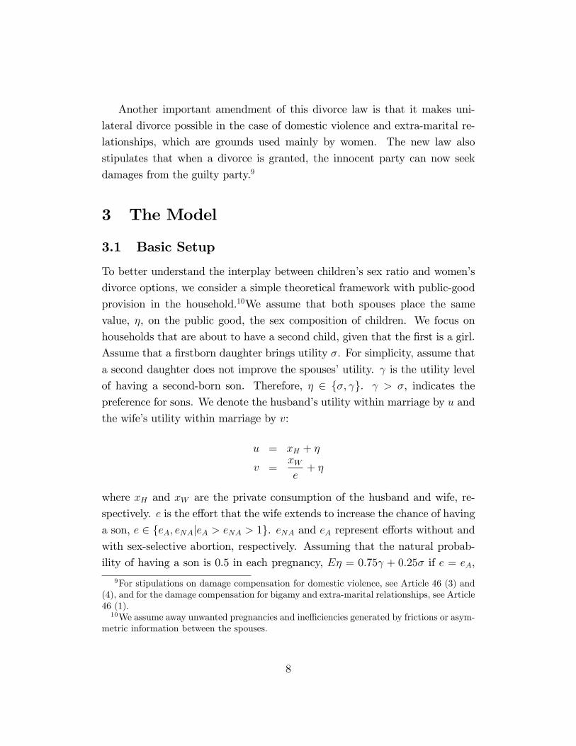
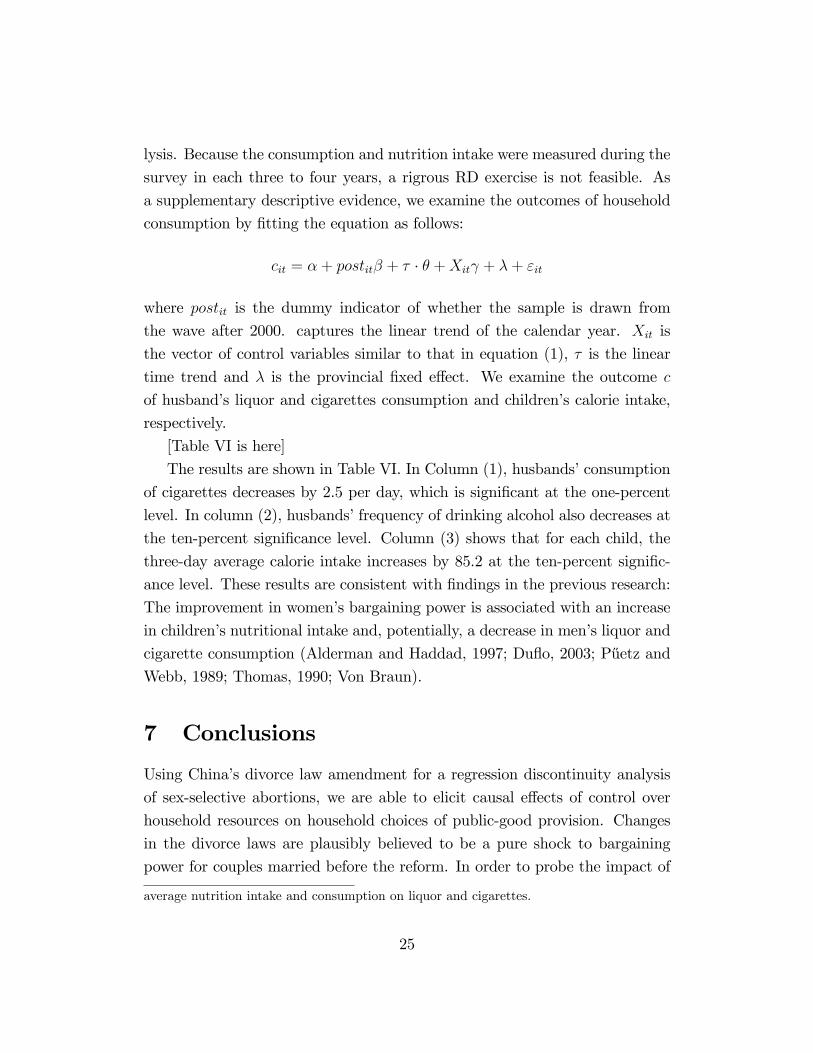
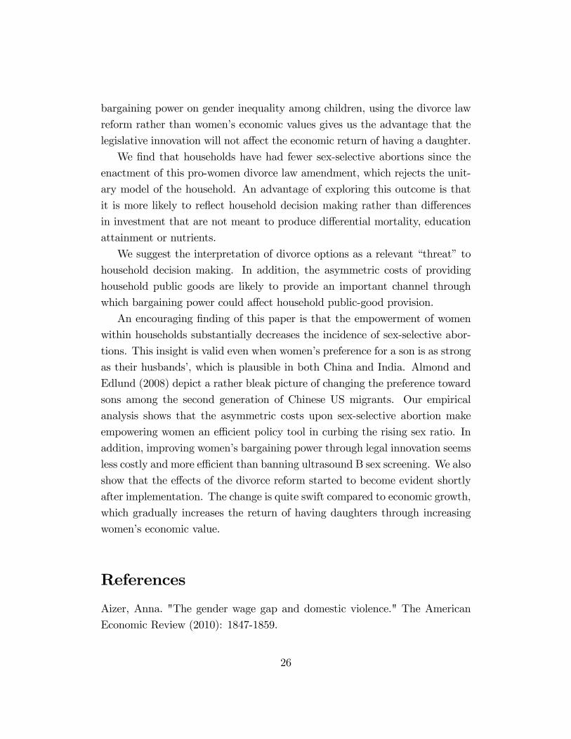
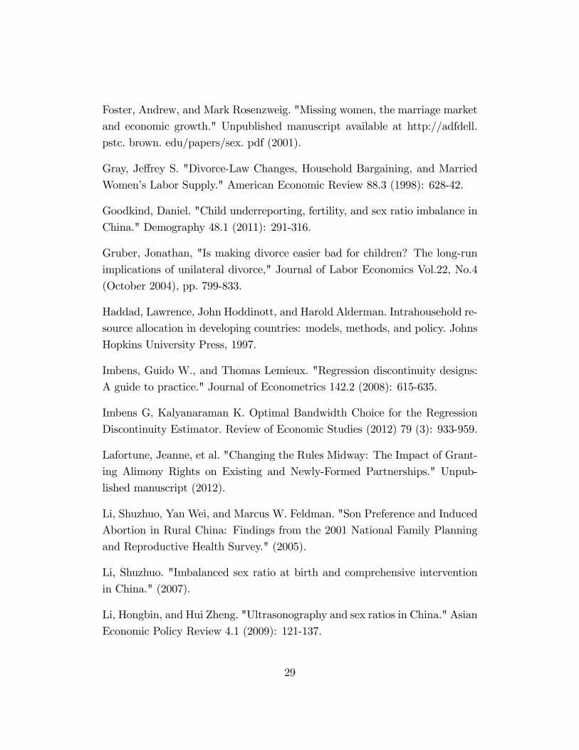
[Figure IA is here]
Figure IA depicts the utility Pareto frontier (UPF) upon abortion and
non-abortion. The horizontal axis is the wife�s utility within marriage, which
equals the reservation utility upon divorce; EuA (vd) has a higher slope than
uNA�vd�because it is more expensive to compensate the wife to vd� cW when
the wife exerts more e¤ort to have a sex-selective abortion. Lines EuA (vd)
and uNA�vd�will intersect if eA is large enough compared to eNA. That is,
eA >2M+ +�
2M+2��( ��)eNA eNA . Denote the value of vd at the intersection of lines
EuA (vd) and uNA�vd�as v̂, v̂ = cW +
( +�)eA�2�eNA+ ��2(eA�eNA) .
10
In Figure IA, if vd < v̂, the UPF upon abortion (EuA (vd)) falls outside that
upon non-abortion (uNA�vd�), and such a household should choose abortion;
when vd > v̂, the UPF upon abortion (EuA (vd)) falls inside that upon non-
abortion (uNA�vd�), and such a household should choose non-abortion.
3.3 Comparative statics and main predictions
The amended divorce law causes a decrease in cW . Since
@v̂
@cW> 0
, as cW decreases, the cuto¤ value of vd decreases. Given women�s intrinsic
divorce option distribution f (vd), there will be households shifting from abor-
tion to non-abortion. In Figure I.A, the intersection (together with the UPFs)
shifts left relative to f (vd).14 Households with vd around cuto¤ v̂ will shift
from abortion to non-abortion. We state this in the proposition, as follows:
Proposition 1 The incidence of sex-selective abortion decreases with the im-provement in women�s divorce options.
To understand the intuition of this proposition, note that the husband faces
the tradeo¤ between sacri�cing more private consumption (the marginal cost
is (vd � cW � �) (eA � eNA)� 0:5eA ( � �)) and having a more preferable sexcomposition of children (the marginal bene�t is 0:5eA ( � �)). The increasein vd�cW increases the marginal cost of sex-selective abortion for the husband,and he could switch from choosing abortion to choosing non-abortion.
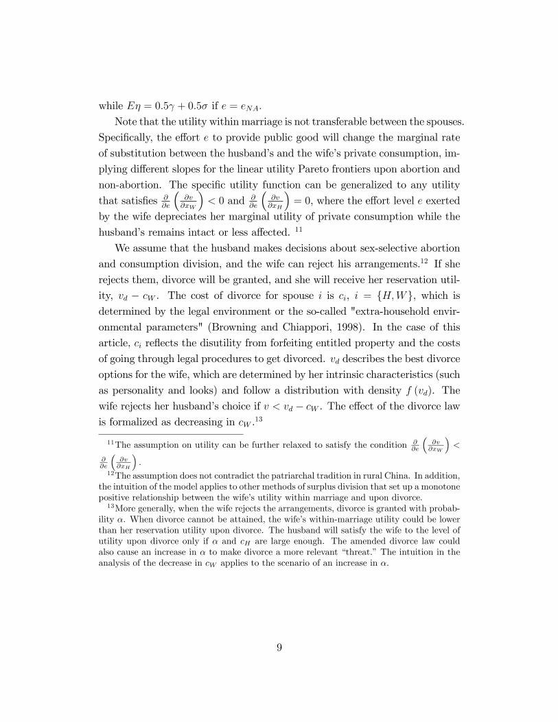
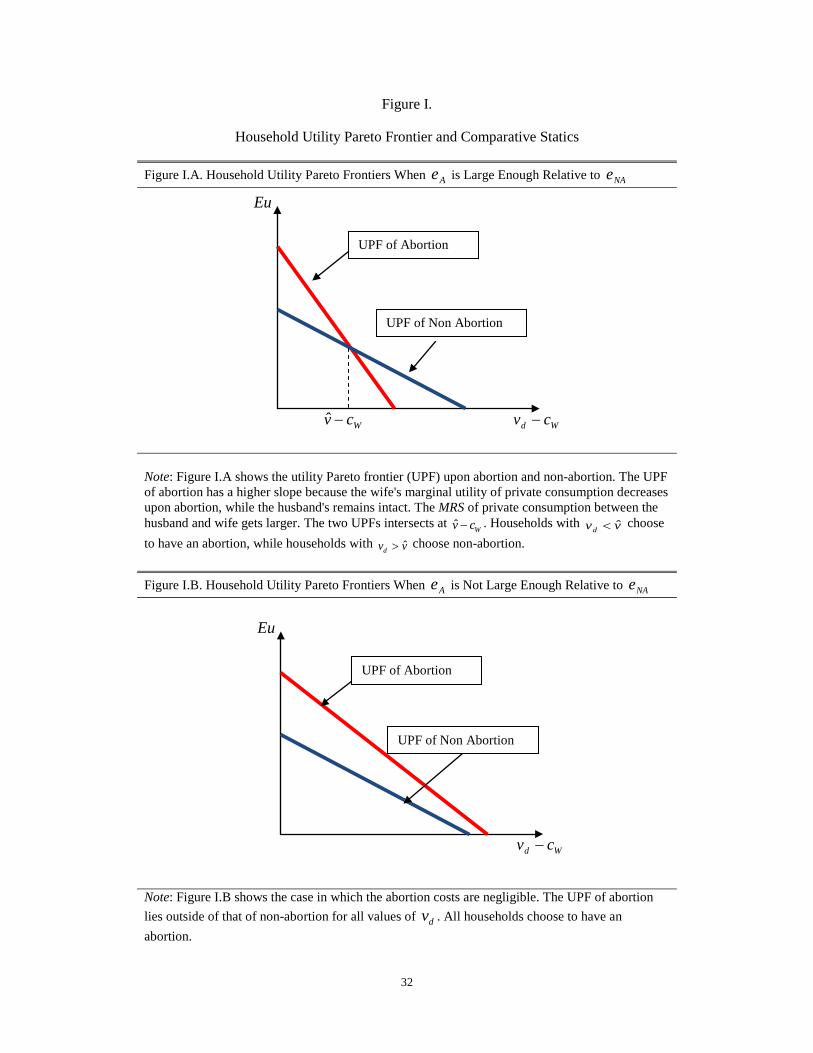
[Figure IB is about here]
To derive an additional testable prediction of the model, we consider vari-
ations in the level of e¤ort required for abortion, eA, in relation to non-abortion
eNA. We relax the prior assumption and allow for eA <2M+ +�
2M+2��( ��)eNA eNA.
This situation is illustrated in Figure I.B, where the UPFs of abortion and
non-abortion, EuA (vd) and uNA (vd), do not intersect, and the UPF of abor-
tion dominates that of non-abortion. The comparison between Figure I.A and14Equivalently, given the position of the UPFs, in Figure I.A, the decrease in cW can be
regarded as shifting the distribution f (vd) rightward.
11
I.B underscores the importance of the wife�s health-related costs in decision
making upon sex-selective abortions.
Corollary 1 All else equal, women with a larger eA relative to eNA are morelikely to respond to the improved divorce options, and household demand for
sex-selective abortions in such families is likely to decrease.
4 Data and Regression Discontinuity Estima-
tion
4.1 Data and Graphical Findings
The empirical analysis of this study compares the sex ratio of the second
children following �rstborn girls shortly before and after the de facto enactment
of the amended divorce law.
The empirical analysis of children�s sex ratio uses the 25-percent sample
of the 2005 One-Percent Population Survey. The Survey contains questions
on sex, date of birth, marital status, date of �rst marriage, educational at-
tainment, migration, and relationship to the head of household. The sample
is limited to the second birth, conditional on a �rstborn daughter, with rural
residency status (hukou). We further con�ne the sample to couples married
before the divorce law amendment to avoid the potential complication that the
law could a¤ect intra-household allocation through a¤ecting marriage match-
ing (Lafortune et al., 2012).
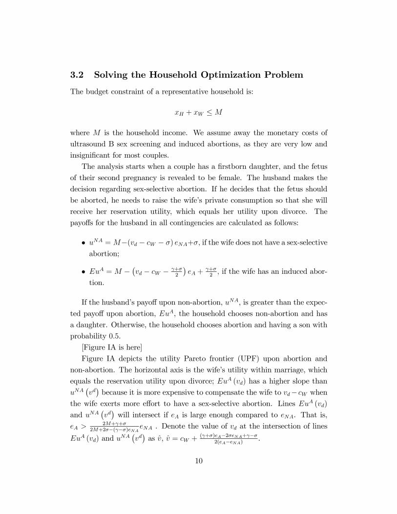
Table I summarizes the descriptive statistics on the ratio of male births
after a �rstborn girl and the personal characteristics of the couple. In Figure
II.A, we categorize children into di¤erent cohorts by the timing of conception
(nine months before birth) and compare the sex ratio of cohorts conceived
before and after the implementation of the new divorce law. Sex ratio is de�ned
as the number of boys to the number of girls. Figure II.A reports the sample
mean of sex ratio by cohort. Each cohort is de�ned as all babies conceived in
each six-month period following February 1997. As is evident from Figure IIA,
within the data period, we observe a marked decline in children�s sex ratio,
12
down from a high point of 2.4 for babies conceived between August 1998 and
January 1999 to a low point of 1.7 for conceptions between February and July
2004. The red line marks the cohort conceived between February and July
2002, which is where the sharp decline takes place.
[Table I is here]
[Figure II.A is here]
To estimate the signi�cance level of this decline in Figure II.A, we �t the
following OLS regression:
Maleic = �+15Xl=1
1[c = l]�l +Xic + �+ "ic (1)
The dependent variable is a dummy indicator of whether child i is male.
Male = 1 if the child is male, 0 otherwise. Each l represents a cohort in Figure
II.A.Xic is the vector of control variables, including the parental characteristics
listed in Table 1. � is the province �xed e¤ect. The �rst cohort in Figure II.A
(i.e., the cohort conceived between February and July 1997) is the reference
group.
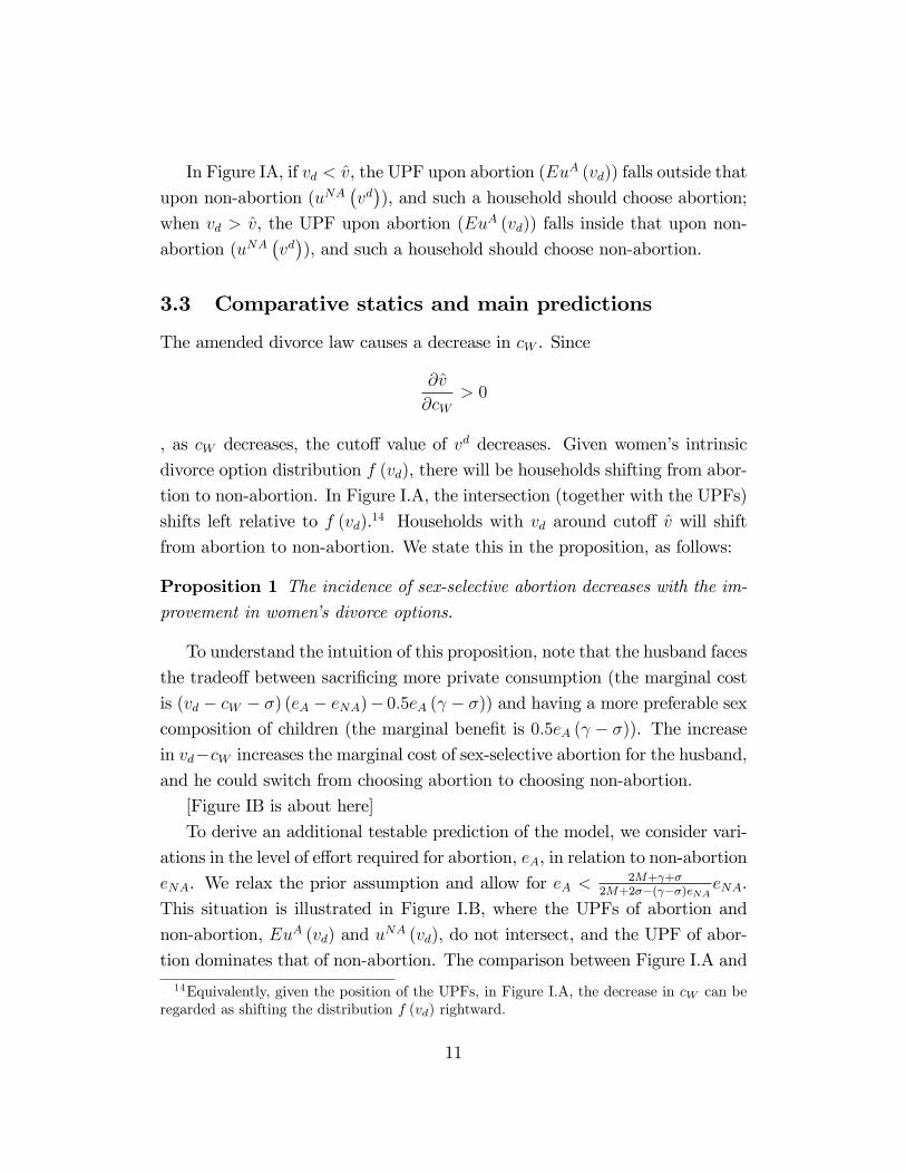
The empirical results of equation (1) are shown in Figure II.B. The circles
are the coe¢ cients of the cohort indicators, with the magnitude labeled in the
�gure. The lines are the 95-percent con�dence interval. In Figure II.B, the
95-percent con�dence intervals start to be consistently below 0 from the cohort
conceived during the six-month period between February and July 2002. The
decline in the propensity to have a second-born son after a �rstborn daugh-
ter is about six percentage points, meaning that the sex ratio has declined
from 2.3-2.3 boys to one girl to 1.56-1.6 boys to one girl since the reform�s
implementation, holding other factors constant.
[Figure II.B is here]
4.2 Graphical Evidence on Causal Relationship
Figures II.A and II.B show that a sharp decline appears at the cohort that was
conceived during the six-month period between February and July 2002. The
sharp decline within a short time period seems to suggest a discrete change in
13
the sex ratio (or a break in the trend) shortly after the implementation of the
divorce reform at the end of December 2001. In other words, the graphical
descriptions indicate a clear timing threshold from which the sex ratio started
to be a¤ected. If such a timing threshold exists, and if it is consistent with that
of the divorce reform implementation, it will be credible to establish a causal
link between the reform and a more-balanced sex ratio. Moreover, we will be
able to apply a more rigorous study design of regression discontinuity (RD) to
estimate the e¤ect of divorce reform at the timing threshold. The RD estimand
can be regarded as a lower bound of the divorce reform�s e¤ect because given
a longer period of time, more households could be able to respond to the
intervention.
We apply an exercise by Chay, McEwan, and Urquiola (2005) to look for
the conception-timing threshold. As previously mentioned, the divorce law
amendment was announced on April 28, 2001 and the judicial interpretation
on December 26, 2001. The dissemination and assimilation of the information
took time; thus, the de facto timing threshold when households started to
respond to the amendment is known with error. We run 92 regressions in total.
Each includes a di¤erent indicator of "conceived in month l or after," where
l represents the exact month of conception during the 93 months between
August 1997 and May 2004. The regression is as follows:
Maleic = �+ 1[c � l]�l +Xic + �+ "ic (2)
with all other features similar to those in equation (1).
Suppose that there exists a clear timing threshold at conception time l�,
when the sex ratio started to be a¤ected. The correlation between the sex
ratio and the proxy variable should be the strongest in the regression with
the dummy indicator 1[c � l�], and, therefore, �l� has the largest magnitudeof t-ratio compared with that in regressions using other cuto¤ indicators. In
addition, the adjusted R-squared should peak in the regression where the
magnitude of the t-ratio yields the maximum. Moreover, we should be able to
observe a �concave�pattern for both the sequence of the magnitude of t-ratios
and the adjusted R-squared. This is because the farther away the assumed
14
cuto¤ is from the real timing threshold l�, the weaker are the explanatory
power of that assumed cuto¤ and the correlation between that cuto¤ and the
sex ratio. Note that if the magnitudes of the adjusted R-squared and the
t-ratio show a concave pattern, we can rule out a common time trend of the
sex ratio. If the detected timing threshold of conception matches the timing
of the new law�s implementation, we can to a large extent rule out the e¤ects
of other policies.
We graph the adjusted R-squared of the sequence of regressions and the
t-ratio magnitude of the coe¢ cient of dummy indicator �conceived in month
l or later�in Figures III.A and III.B.
[Figure III.A is here]
[Figure III.B is here]
As the �gures show, the magnitudes of the adjusted R-squared and the
t-ratio of the coe¢ cient of the threshold peak in the same regression when
using the conception timing February 2002 as the cuto¤ in equation (2). The
adjusted R-squared and the t-ratio not only attain maximum magnitude in
the regression using February 2002 as the cuto¤, but the magnitudes of the
R-squared and the t-ratio also show a �concave� pattern. Speci�cally, in
Figure III.A, the adjusted R-squared increases when the cuto¤ approaches
the threshold February 2002, and it decreases when the cuto¤ is de�ned as
an earlier or later date. The adjusted R-squared gets smaller because more
�noise� is added to the �real� threshold. A similar pattern is observed in
Figure III.B when examining the magnitude of t-ratio of the sequence of the
cuto¤s�coe¢ cients.
The threshold is, to a large extent, consistent with the timing of the imple-
mentation of the divorce law. In addition, the �concave pattern�shows that
it is unlikely that a time trend is driving the decline in children�s sex ratio.
4.3 Regression Discontinuity Estimation
To identify the e¤ect of the divorce reform, with the timing threshold detected,
we adopt a reduced-form non-parametric RD design. In this design, the jump
in the regression of the dummy variable indicating whether the child is male
15
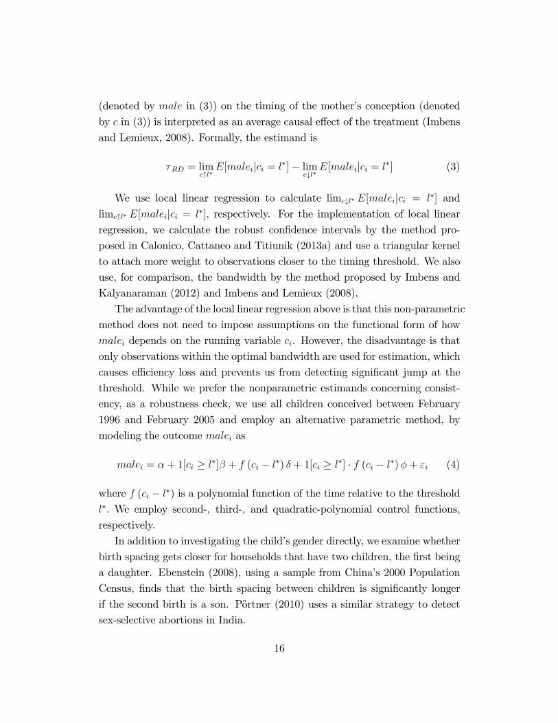
(denoted by male in (3)) on the timing of the mother�s conception (denoted
by c in (3)) is interpreted as an average causal e¤ect of the treatment (Imbens
and Lemieux, 2008). Formally, the estimand is
�RD = limc"l�E[maleijci = l�]� lim
c#l�E[maleijci = l�] (3)
We use local linear regression to calculate limc#l� E[maleijci = l�] and
limc"l� E[maleijci = l�]; respectively. For the implementation of local linear
regression, we calculate the robust con�dence intervals by the method pro-
posed in Calonico, Cattaneo and Titiunik (2013a) and use a triangular kernel
to attach more weight to observations closer to the timing threshold. We also
use, for comparison, the bandwidth by the method proposed by Imbens and
Kalyanaraman (2012) and Imbens and Lemieux (2008).
The advantage of the local linear regression above is that this non-parametric
method does not need to impose assumptions on the functional form of how
malei depends on the running variable ci. However, the disadvantage is that
only observations within the optimal bandwidth are used for estimation, which
causes e¢ ciency loss and prevents us from detecting signi�cant jump at the
threshold. While we prefer the nonparametric estimands concerning consist-
ency, as a robustness check, we use all children conceived between February
1996 and February 2005 and employ an alternative parametric method, by
modeling the outcome malei as
malei = �+ 1[ci � l�]� + f (ci � l�) � + 1[ci � l�] � f (ci � l�)�+ "i (4)
where f (ci � l�) is a polynomial function of the time relative to the thresholdl�: We employ second-, third-, and quadratic-polynomial control functions,
respectively.
In addition to investigating the child�s gender directly, we examine whether
birth spacing gets closer for households that have two children, the �rst being
a daughter. Ebenstein (2008), using a sample from China�s 2000 Population
Census, �nds that the birth spacing between children is signi�cantly longer
if the second birth is a son. P½ortner (2010) uses a similar strategy to detect
sex-selective abortions in India.
16

[Figure IV is here]
[Table II is here]
Figure IV plots the probability that the second child after a �rstborn
daughter is a son, according to the mother�s conception month relative to
the timing threshold (=0 if the child is conceived in February 2002). The
circles are the average of the dummy indicator of being a son for groups of
children, de�ned by the conception months relative to the threshold February
2002. In addition, we present the smoothed values from a kernel-weighted
local polynomial regression of the dummy indicator of the second child being
a son on the relative month at the left and right side of the cuto¤, respect-
ively. Together, we plot the 95-percent con�dence band. Figure IV shows the
drop-o¤ of the dummy indicator for the child being a son at the time when
the divorce reform took e¤ect.
Table II, Columns (1)-(3) report the estimands using di¤erent bandwidth
selectors, showing that the decrease at the timing cuto¤ is consistently signi-
�cant at the one-percent level. When the bandwidth is con�ned to the nine
months around the threshold, the decline in the propensity to have a son after
a �rstborn girl amounts to 8.9 percentage points. Columns (4)-(6) report
the OLS estimation with second-, third- and fourth-order polynomial control
functions, respectively. The entries show that the jump at the threshold is
signi�cant at the �ve-percent level.
[Figure V is here]
[Table III is here]
Figure V plots birth spacing between the �rst and second child against
mother�s relative conception month. The circles are the average of birth spa-
cing in each conception month. The curves are the smoothed values from a
kernel-weighted local polynomial regression of the birth spacing on the relative
month at the left and right side of the cuto¤, respectively. The entries in Table
III, Columns (1)-(3) report that the estimands using di¤erent bandwidth se-
lectors are signi�cant at the �ve-percent level. Within the bandwidth of eleven
months around the threshold, birth spacing decreased by 3.386 months, which
is comparable to the estimand by Ebeinstein (2008). Using the whole sample
comprised of all second-born children conceived after February 1996, Columns
17
(4)-(6) show the OLS estimation with di¤erent-order polynomial control func-
tions.
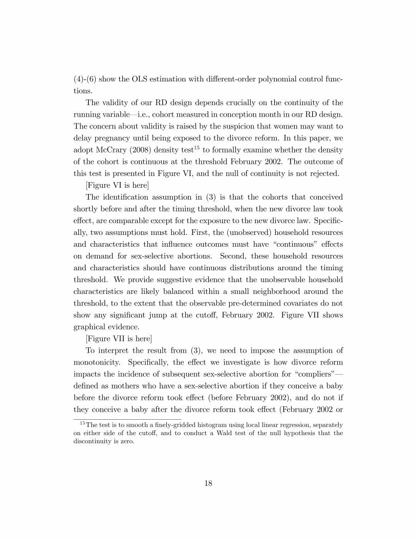
The validity of our RD design depends crucially on the continuity of the
running variable� i.e., cohort measured in conception month in our RD design.
The concern about validity is raised by the suspicion that women may want to
delay pregnancy until being exposed to the divorce reform. In this paper, we
adopt McCrary (2008) density test15 to formally examine whether the density
of the cohort is continuous at the threshold February 2002. The outcome of
this test is presented in Figure VI, and the null of continuity is not rejected.
[Figure VI is here]
The identi�cation assumption in (3) is that the cohorts that conceived
shortly before and after the timing threshold, when the new divorce law took
e¤ect, are comparable except for the exposure to the new divorce law. Speci�c-
ally, two assumptions must hold. First, the (unobserved) household resources
and characteristics that in�uence outcomes must have �continuous� e¤ects
on demand for sex-selective abortions. Second, these household resources
and characteristics should have continuous distributions around the timing
threshold. We provide suggestive evidence that the unobservable household
characteristics are likely balanced within a small neighborhood around the
threshold, to the extent that the observable pre-determined covariates do not
show any signi�cant jump at the cuto¤, February 2002. Figure VII shows
graphical evidence.
[Figure VII is here]
To interpret the result from (3), we need to impose the assumption of
monotonicity. Speci�cally, the e¤ect we investigate is how divorce reform
impacts the incidence of subsequent sex-selective abortion for �compliers��
de�ned as mothers who have a sex-selective abortion if they conceive a baby
before the divorce reform took e¤ect (before February 2002), and do not if
they conceive a baby after the divorce reform took e¤ect (February 2002 or
15The test is to smooth a �nely-gridded histogram using local linear regression, separatelyon either side of the cuto¤, and to conduct a Wald test of the null hypothesis that thediscontinuity is zero.
18
later). Then,
�RD = limc#l�E[maleijci = l�]� lim
c"l�E[maleijci = l�] (5)
= E[malei (1)�malei (0) j i is a complier and ci = l�]
wheremalei (1) denotes the child i�s sex when the mother�s conception happened
after the timing threshold, and malei (0) denotes the child i�s sex when the
mother�s conception happened before the timing threshold. In addition, we
regard E[malei (1)�malei (0) j i is a complier and ci = l�] as the lower boundof the divorce reform�s average e¤ect because information about the reform is
likely to reach more households and be better understood later (when l > l�).
Another concern regarding the interpretation is that the analysis of chil-
dren�s gender uses information on surviving children reported by their parents.
This sex ratio could be di¤erent from the sex ratio at birth because the decline
in the former may also be driven by the decreasing gender di¤erence in the
mortality rates for young children, or by the decreasing propensity to underre-
port female births. Much of the previous research shows that the skewed sex
ratio of children is caused mainly by sex-selective abortions. Zeng (1993) rules
out the likelihood of infanticide using data from multiple sources. Goodkind
(2011) analyzes China�s 2000 Census data and �nds that given excess underre-
porting of young daughters, especially pronounced just after 1990, estimated
sex ratios are lower than reported ratios.16 We �nd no nationwide policies
in the relevant time window that could have caused a systematic decrease in
underreporting female births. We also �nd no factors that would mitigate the
misreporting incentive, speci�cally for children conceived after the detected
timing threshold. One concern is that, if there is a secular trend or life-cycle
pattern of such underreporting, our RD estimands could be contaminated if
the RD design fails to drop it out, especially when the bandwidth is large.
However, Zeng (1993) �nds that underreporting of female children is more
common for newborns or very young children because �hiding�a child will be
more costly as she grows older. In this article, we �nd that the sex ratio is
16Goodkind (2011) �nds that China�s sex ratio at birth, once it is standardized by birthorder, fell between 2000 and 2005, which is consistent with our �ndings.
19
more balanced among younger cohorts, which could only be underestimated if
underreporting female children could possibly a¤ect the RD estimand.
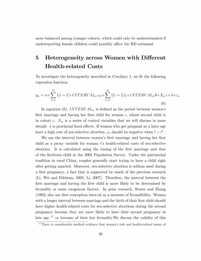
5 Heterogeneity across Women with Di¤erent
Health-related Costs
To investigate the heterogeneity described in Corollary 1, we �t the following
regression function:
yic = �+15Xl=1
1[c = l]�INTERV ALic�!l+15Xl=1
1[c = l]�l+INTERV ALic�+Xic +�+"ic
(6)
In equation (6), INTERV ALic is de�ned as the period between women�s
�rst marriage and having her �rst child for woman i, whose second child is
in cohort c. Xic is a series of control variables that we will discuss in more
details. � is provincial �xed e¤ects. If women who get pregnant at a later age
have a high cost of sex-selective abortion, !l should be negative when l > l�.
We use the interval between women�s �rst marriage and having her �rst
child as a proxy variable for woman i�s health-related costs of sex-selective
abortion. It is calculated using the timing of the �rst marriage and that
of the �rstborn child in the 2005 Population Survey. Under the patriarchal
tradition in rural China, couples generally start trying to have a child right
after getting married. Moreover, sex-selective abortion is seldom used during
a �rst pregnancy, a fact that is supported by much of the previous research
(Li, Wei and Feldman, 2005; Li, 2007). Therefore, the interval between the
�rst marriage and having the �rst child is more likely to be determined by
fecundity or some exogenous factors. In prior research, Sturm and Zhang
(1993) also use �rst conception interval as a measure of fecundibility. Women
with a longer interval between marriage and the birth of their �rst child should
have higher health-related costs for sex-selective abortions during the second
pregnancy because they are more likely to have their second pregnancy in
late age 17 or because of their low fecundity.We discuss the validity of this17There is considerable medical evidence that women�s risk and health-related issues of
20
proxy variable from three aspects. First, the interval between marriage and
�rst birth may not capture only fecundity. If women with a better bargaining
position tend to have their �rst child late and are closer to the margin to
be a¤ected by the divorce reform, then the negative correlation between the
length of the interval and the magnitude of the divorce reform�s e¤ect can
be explained by the di¤erence in initial bargaining power. Second, fecundity
could be the consequence of marriage matching if women�s fecundity can be
observed in marriage market or is closely related with observable factors valued
in marriage market. Therefore, a household with a fertile wife may not be
perfectly comparable to that with a less-fertile wife. Third, fecundity, per se,
could a¤ect women�s bargaining position within a household.
We address these related concerns in a few ways. First, we control variables
that could capture initial bargaining power and matching quality, including the
education and age at the time of �rst marriage for both spouses. In particular,
since women�s age at �rst marriage is generally regarded as a strong indicator
of bargaining position, to address the concern that the heterogeneity could
be driven by the di¤erence in initial bargarning position, we also control the
interactions of age at �rst marriage and the dummy indicator of having a
second child after the divorce reform. Second, we exclude the individual with
the longest quartile of this interval. The intervals in the top quartile are longer
than four years. We may suspect that for these women, the timing of having
their �rst child could be a consequence of optimizing the trajectory of their
career development, or they may not make a good comparison with those
who have their �rst child soon after marriage. Finally, we argue that if low
fecundity causes a decrease in women�s bargaining position, the heterogeneity
proposed in the model will be underestimated.
[Table IV and Table V are here]
Table IV, Columns (1)-(3) report the results of the speci�cation of con-
trolling provincial �xed e¤ects, adding more controls for parental education,
ethnicity, age at �rst marriage and indicators of migrants, respectively. Prior
pregnancy and sex-selective abortion increase with the age at which she becomes pregnant.Complications include elevated blood pressure, gestational diabetes, premature labor, andbleeding disorders such as placental abruption, etc.
21
research (Bates et al., 2004; Field and Ambrus 2008) show that women�s edu-
cation levels and age at marriage are likely to be associated with their position
in the marriage. Parents�migration status could potentially a¤ect sex selection
because some migration could be driven by the incentive to escape from the
restrictions of their local family-planning policies. Table IV shows that women
who are older at �rst pregnancy are less likely than those who are younger to
have a second-born son after having a �rstborn daughter. Speci�cally, a one-
year increase in the interval between marriage and the �rst birth decreases the
probability of having a second-born son by 1.5 to 2.4 percentage points. This
is consistent with Corollary 1, in that households become more responsive to
the divorce law when women�s health-related costs of sex-selective abortions
are large enough. This is the case because the couple will not make a (joint)
decision to exert a costly e¤ort when it sacri�ces too much of the husband�s
private consumption.
In Column (4), we con�ne the sample to women whose time between their
�rst marriage and having their �rst child is shorter than four years, the 75th
percentile. By focusing on this subsample, we exclude, to an extent, those who
intend to delay having children. The coe¢ cients are of similar magnitudes and
similar signi�cance levels. The robustness of the result shown in column (4)
suggests that the variation in the time interval that we use for identi�cation
is largely exogenous. Speci�cally, it is unlikely to be driven by women�s op-
timization or to be related to women�s bargaining power.
Regarding the outcome of birth spacing, the �rst three columns of Table
V show that birth spacing decreases by around 0.4-0.6 months following the
divorce reform when the woman�s age when having her �rst child increases
by one year. The coe¢ cients are of similar magnitude when the sample is
con�ned to women with a shorter time span between their �rst marriage and
having their �rst child (column (4)).
22
6 Robustness and Supplementary Results
6.1 Other Policies
To exclude the possibility that policies other than the new divorce law could
drive the discrete change in children�s sex and induced abortions, we conduct
an exhaustive search of all policy changes in the relevant time window.
In December 2001, the central government announced that the �Law of
Population and Family Planning" (LPFP) was to replace the previous �Reg-
ulation of Population and Family Planning�to govern family planning. The
contents of the two documents are essentially the same, except that the LPFP
is enforceable by the court.18 Nevertheless, some skepticism is warranted be-
cause a law generally means stricter enforcement than a policy, and our de-
tected timing threshold is close to the timing of the LPFP announcement.
Therefore, we examine whether the LPFP caused the discontinuity.
Unlike the divorce reform, which took e¤ect nationwide immediately fol-
lowing its enactment, due to large preexisting di¤erences in family-planning
policies across provinces, LPFP let each province decide on the timing and
speci�cs of a local policy change relative to its original family-planning policy.
Consequently, the implementation took place between September 2002 and
April 2004 (See Appendix Table I), a period that was after our discontinuity
threshold. To show that the discrete change in the sex ratio should not be
attributed to LPFP, we conduct a discontinuity analysis by plotting children�s
sex ratio against the conception month relative to the implementation dates
on left and right side of the implementation cuto¤, respectively. Figure VIII
clearly shows that there is no discontinuity at the time of the enactment of
the provincial Act of Population and Family Planning.
18The "Act of Population and Family Planning" has been slightly changed in someprovinces. For example, in Hubei province, the 1987 version of the Act states that "thecouple is quali�ed to have a second child if one party of the spouses is disabled." This art-icle was reversed in the December 2002 Act. In the 1987 Act, a remarried couple is quali�edto have one child of their own only if one party has had no child and the other party has hadno more than one child. The 2002 Act relaxed these rules a little: If one party is widowedbefore the current marriage, and the other party has had no child before, the spouses arequali�ed to have their own child even if the widowed party had two children in the previousmarriage.
23
[Figure VIII is here]
Following LPFP, the central government announced two more documents
to strengthen enforcement of the ban on sex-selective abortions stated in
LPFP: "The Prohibition of Ultrasound B Sex Screening and Induced Abor-
tions" and "The Comprehensive Views on Curbing the Rising Sex Ratio,"
which were announced in January and June 2003, respectively. The two doc-
uments cannot cause the detected discontinuity because the announcements
were even later than the period discussed above.
Another potentially relevant program is the "Care for Girls Program"
(Guan Ai Nv Hai Xing Dong), which was initiated in 2003, aiming to mit-
igate discrimination against women and girls and eventually curb the rising
sex ratio at birth. However, until February 2004, the program covered only
11 counties (among the 1,463 counties in China). Therefore, the nationwide
decline in the sex ratio is not likely to be driven by this program.
6.2 Supplementary Evidence on Women�s BargainingPower Improvement
In this section, we show the improvement in women�s bargaining power in such
areas as household consumption. Our model suggests that women�s private
consumption could go either way following fewer sex-selective abortions. If the
household decision switches from abortion to non-abortion, the wife�s marginal
utility of consumption is greater, which means that she is able to attain the
same level of utility with less consumption. Thus, her consumption could be
lower than it was before the improvement in divorce options. Therefore, we fo-
cus on households that are already done having children. For these households,
fertility or sex-selective abortions are pre-determined, and improvement in the
wife�s utility within marriage can be unambiguously re�ected by an increase
in her consumption.
We use China�s Health and Nutrition Survey (CHNS) data19 for this ana-
19CHNS was administered by the Population Center at the University of North Carolina in1991, 1993, 1997, 2000, 2004, 2006, 2009 and 2011.The survey took place over a 3-day periodusing a multistage, random cluster process to draw a sample of about 4400 households witha total of 26,000 individuals in nine provinces. CHNS has detailed information on three-day
24
lysis. Because the consumption and nutrition intake were measured during the
survey in each three to four years, a rigrous RD exercise is not feasible. As
a supplementary descriptive evidence, we examine the outcomes of household
consumption by �tting the equation as follows:
cit = �+ postit� + � � � +Xit + �+ "it
where postit is the dummy indicator of whether the sample is drawn from
the wave after 2000. captures the linear trend of the calendar year. Xit is
the vector of control variables similar to that in equation (1), � is the linear
time trend and � is the provincial �xed e¤ect. We examine the outcome c
of husband�s liquor and cigarettes consumption and children�s calorie intake,
respectively.
[Table VI is here]
The results are shown in Table VI. In Column (1), husbands�consumption
of cigarettes decreases by 2.5 per day, which is signi�cant at the one-percent
level. In column (2), husbands�frequency of drinking alcohol also decreases at
the ten-percent signi�cance level. Column (3) shows that for each child, the
three-day average calorie intake increases by 85.2 at the ten-percent signi�c-
ance level. These results are consistent with �ndings in the previous research:
The improvement in women�s bargaining power is associated with an increase
in children�s nutritional intake and, potentially, a decrease in men�s liquor and
cigarette consumption (Alderman and Haddad, 1997; Du�o, 2003; P½uetz and
Webb, 1989; Thomas, 1990; Von Braun).
7 Conclusions
Using China�s divorce law amendment for a regression discontinuity analysis
of sex-selective abortions, we are able to elicit causal e¤ects of control over
household resources on household choices of public-good provision. Changes
in the divorce laws are plausibly believed to be a pure shock to bargaining
power for couples married before the reform. In order to probe the impact of
average nutrition intake and consumption on liquor and cigarettes.
25
bargaining power on gender inequality among children, using the divorce law
reform rather than women�s economic values gives us the advantage that the
legislative innovation will not a¤ect the economic return of having a daughter.
We �nd that households have had fewer sex-selective abortions since the
enactment of this pro-women divorce law amendment, which rejects the unit-
ary model of the household. An advantage of exploring this outcome is that
it is more likely to re�ect household decision making rather than di¤erences
in investment that are not meant to produce di¤erential mortality, education
attainment or nutrients.
We suggest the interpretation of divorce options as a relevant �threat�to
household decision making. In addition, the asymmetric costs of providing
household public goods are likely to provide an important channel through
which bargaining power could a¤ect household public-good provision.
An encouraging �nding of this paper is that the empowerment of women
within households substantially decreases the incidence of sex-selective abor-
tions. This insight is valid even when women�s preference for a son is as strong
as their husbands�, which is plausible in both China and India. Almond and
Edlund (2008) depict a rather bleak picture of changing the preference toward
sons among the second generation of Chinese US migrants. Our empirical
analysis shows that the asymmetric costs upon sex-selective abortion make
empowering women an e¢ cient policy tool in curbing the rising sex ratio. In
addition, improving women�s bargaining power through legal innovation seems
less costly and more e¢ cient than banning ultrasound B sex screening. We also
show that the e¤ects of the divorce reform started to become evident shortly
after implementation. The change is quite swift compared to economic growth,
which gradually increases the return of having daughters through increasing
women�s economic value.
References
Aizer, Anna. "The gender wage gap and domestic violence." The American
Economic Review (2010): 1847-1859.
26

Almond, Douglas, and Lena Edlund. "Son-biased sex ratios in the 2000 United
States Census." Proceedings of the National Academy of Sciences 105.15
(2008): 5681-5682.
Arnold, Fred, Minja Kim Choe, and T. K. Roy. "Son preference, the family-
building process and child mortality in India." Population studies 52.3 (1998):
301-315.
Bates, Lisa M., Farzana Islam, Khairul Islam, and Sidney Ruth Schuler.
2004.�Legal Registration of Marriage in Bangladesh: An Intervention to
Strengthen Women�s Economic and Social Position and Protect Them against
Domestic Violence?�Manuscript, Acad. Educ. Development, Washington, DC.
Banerjee, Abhijit V. "Educational Policy and the Economics of the Fam-
ily."Journal of Development Economics 74.1 (2004): 3-32.
Ben-Porath, Yoram. "The production of human capital and the life cycle of
earnings." The Journal of Political Economy (1967): 352-365.
Ben-Porath, Voram. "Short-term �uctuations in fertility and economic activity
in Israel." Demography 10.2 (1973): 185-204.
Ben-Porath, Yoram, and Finis Welch. "Do sex preferences really matter?."
The Quarterly Journal of Economics 90.2 (1976): 285-307.
Blundell, Richard, Pierre-André Chiappori, and Costas Meghir. "Collective
labor supply with children." Journal of Political Economy 113.6 (2005): 1277-
1306.
Browning, Martin, and Pierre-Andre Chiappori. "E¢ cient intra-household
allocations: A general characterization and empirical tests." Econometrica
(1998): 1241-1278.
Burgess, Robin, and Juzhong Zhuang. "Modernisation and son preference."
(2000).
27

Calonico, Sebastian, Matias D. Cattaneo, and Rocio Titiunik. "Robust non-
parametric con�dence intervals for regression-discontinuity designs." Revision
requested by Econometrica (2013).
Chay, Kenneth Y., Patrick J. McEwan, and Miguel Urquiola. "The Cent-
ral Role of Noise in Evaluating Interventions That Use Test Scores to Rank
Schools." American Economic Review 95.4 (2005): 1237-1258.
Chiappori, Pierre-André, Murat Iyigun, and YoramWeiss. Public goods, trans-
ferable utility and divorce laws. No. 2646. IZA Discussion Papers, 2007.
Chiappori, Pierre-André, Yoram Weiss, "Divorce, Remarriage and Welfare: A
General Equilibrium Approach " Journal of the European Economic Associ-
ation, 4(2-3), 2006, pp.415-426.
Chu, Junhong. "Prenatal sex determination and sex-selective abortion in rural
central China." Population and Development Review 27.2 (2001): 259-281.
Clark, Shelley. "Son preference and sex composition of children: Evidence from
India." Demography 37.1 (2000): 95-108.
Gupta, Monica Das. "Selective discrimination against female children in rural
Punjab, India." Population and development review (1987): 77-100.
Du�o, Esther. "Grandmothers and Granddaughters: Old Age Pensions and
Intrahousehold Allocation in South Africa." (2003).
Du�o, Esther. "Women Empowerment and Economic Development." Journal
of Economic Literature 50.4 (2012): 1051-79.
Ebenstein, Avraham. "The �missing girls�of China and the unintended con-
sequences of the one child policy." Journal of Human Resources 45.1 (2010):
87-115.
Field, Erica, and Attila Ambrus. "Early marriage, age of menarche, and fe-
male schooling attainment in Bangladesh." Journal of Political Economy 116.5
(2008): 881-930.
28
Foster, Andrew, and Mark Rosenzweig. "Missing women, the marriage market
and economic growth." Unpublished manuscript available at http://adfdell.
pstc. brown. edu/papers/sex. pdf (2001).
Gray, Je¤rey S. "Divorce-Law Changes, Household Bargaining, and Married
Women�s Labor Supply." American Economic Review 88.3 (1998): 628-42.
Goodkind, Daniel. "Child underreporting, fertility, and sex ratio imbalance in
China." Demography 48.1 (2011): 291-316.
Gruber, Jonathan, "Is making divorce easier bad for children? The long-run
implications of unilateral divorce," Journal of Labor Economics Vol.22, No.4
(October 2004), pp. 799-833.
Haddad, Lawrence, John Hoddinott, and Harold Alderman. Intrahousehold re-
source allocation in developing countries: models, methods, and policy. Johns
Hopkins University Press, 1997.
Imbens, Guido W., and Thomas Lemieux. "Regression discontinuity designs:
A guide to practice." Journal of Econometrics 142.2 (2008): 615-635.
Imbens G, Kalyanaraman K. Optimal Bandwidth Choice for the Regression
Discontinuity Estimator. Review of Economic Studies (2012) 79 (3): 933-959.
Lafortune, Jeanne, et al. "Changing the Rules Midway: The Impact of Grant-
ing Alimony Rights on Existing and Newly-Formed Partnerships." Unpub-
lished manuscript (2012).
Li, Shuzhuo, Yan Wei, and Marcus W. Feldman. "Son Preference and Induced
Abortion in Rural China: Findings from the 2001 National Family Planning
and Reproductive Health Survey." (2005).
Li, Shuzhuo. "Imbalanced sex ratio at birth and comprehensive intervention
in China." (2007).
Li, Hongbin, and Hui Zheng. "Ultrasonography and sex ratios in China." Asian
Economic Policy Review 4.1 (2009): 121-137.
29

Cecilia Chan, Liu Meng. "Family violence in China: Past and present." Journal
of Comparative Social Welfare 16.1 (2000): 74-87.
Manser, Marilyn, and Murray Brown. "Marriage and household decision-
making: A bargaining analysis." International economic review (1980): 31-44.
McCrary, Justin. "Manipulation of the running variable in the regression dis-
continuity design: A density test." Journal of Econometrics 142.2 (2008): 698-
714.[34] Manser, Marilyn, Murray Brown, "Marriage and household decision-
making: A bargaining analysis," International Economic Review, 21(1), 1980.
McElroy, Marjorie B., and Mary Jean Horney. "Nash-bargained household
decisions: Toward a generalization of the theory of demand." International
Economic Review 22.2 (1981): 333-349.
McElroy, Marjorie B. "The Empirical Content of Nash-Bargained Household
Behavior." Journal of human resources 25.4 (1990).
Pörtner, Claus C. "Sex selective abortions, fertility and birth spacing." Uni-
versity of Washington, Department of Economics, Working Paper (2010).
Rangel, Marcos A. "Alimony rights and intrahousehold allocation of resources:
Evidence from brazil." The Economic Journal 116.513 (2006): 627-658.
Rohlfs, Chris, Alexander Reed, and Hiroyuki Yamada. "Causal e¤ects of sex
preference on sex-blind and sex-selective child avoidance and substitution
across birth years: Evidence from the Japanese year of the �re horse." Journal
of Development Economics 92.1 (2010): 82-95.
Rosenzweig, Mark R., and T. Paul Schultz. "Market opportunities, genetic
endowments, and intrafamily resource distribution: Child survival in rural
India." The American Economic Review (1982): 803-815.
Sturm, Roland, and Junsen Zhang. "Fecundibility and social development in
China: changes in the distribution of the �rst conception interval." Biometrical
journal 35.8 (1993): 985-995.
30

Qian, Nancy. "Missing women and the price of tea in China: The e¤ect of
sex-speci�c earnings on sex imbalance." The Quarterly Journal of Economics
123.3 (2008): 1251-1285.
Scharping, Thomas. Birth Control in China 1949-2000: Population policy and
demographic development. Routledge, 2003.
Sen, Amartya. "More than 100 million women are missing." The New York
Review of Books 37 (1990).
Sen, Amartya. "Missing women." BMJ: British Medical Journal 304.6827
(1992): 587.
Stevenson, Betsey. "Divorce law and women�s labor supply." Journal of Em-
pirical Legal Studies 5.4 (2008): 853-873.
Stevenson, Betsey, and Justin Wolfers. "Bargaining in the shadow of the law:
Divorce laws and family distress." The Quarterly Journal of Economics 121.1
(2006): 267-288.
Thomas, Duncan. "Intra-Household Resource Allocation An Inferential Ap-
proach." Journal of human resources 25.4 (1990).
Thomas, Duncan, John Strauss, and Maria-Helena Henriques. "How does
mother�s education a¤ect child height?." Journal of human resources (1991):
183-211.
Von Braun, Joachim, Detlev Puetz, and Patrick Webb. Irrigation technology
and commercialization of rice in The Gambia, e¤ects on income and nutrition.
No. 75. Intl Food Policy Res Inst, 1989.
Yi, Zeng, et al. "Causes and implications of the recent increase in the reported
sex ratio at birth in China." Population and Development Review (1993):
283-302.
Zeng, Yi, Deqing Wu, "Regional Analysis of Divorce in China since 1980,"
Demography Vol. 37, No. 2 (May, 2000), pp.215-219.
31
32
Figure I.
Household Utility Pareto Frontier and Comparative Statics
Figure I.A. Household Utility Pareto Frontiers When Ae is Large Enough Relative to NAe
Note: Figure I.A shows the utility Pareto frontier (UPF) upon abortion and non-abortion. The UPF of abortion has a higher slope because the wife's marginal utility of private consumption decreases upon abortion, while the husband's remains intact. The MRS of private consumption between the husband and wife gets larger. The two UPFs intersects at Wcv −ˆ . Households with vvd ˆ< choose to have an abortion, while households with vvd ˆ> choose non-abortion. Figure I.B. Household Utility Pareto Frontiers When Ae is Not Large Enough Relative to NAe
Note: Figure I.B shows the case in which the abortion costs are negligible. The UPF of abortion lies outside of that of non-abortion for all values of dv . All households choose to have an abortion.
Eu
UPF of Abortion
UPF of Non Abortion
Wd cv −
Eu
UPF of Abortion
UPF of Non Abortion
Wd cv − Wcv −ˆ
33
Figure II.
Sex ratio of the Second-born Children after Having Firstborn Daughters
Figure II.A. Sample Mean of Sex Ratio by Cohort
Figure II.B. Coefficient and 95% C.I. of the Cohort indicators
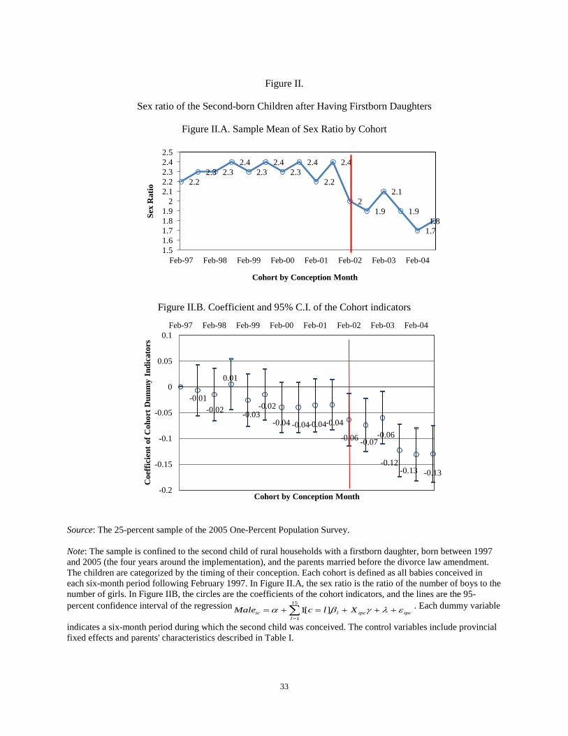
Source: The 25-percent sample of the 2005 One-Percent Population Survey. Note: The sample is confined to the second child of rural households with a firstborn daughter, born between 1997 and 2005 (the four years around the implementation), and the parents married before the divorce law amendment. The children are categorized by the timing of their conception. Each cohort is defined as all babies conceived in each six-month period following February 1997. In Figure II.A, the sex ratio is the ratio of the number of boys to the number of girls. In Figure IIB, the circles are the coefficients of the cohort indicators, and the lines are the 95-percent confidence interval of the regression ∑
=
+++=+=15
1][1
lipcipclic XlcMale ελγβα . Each dummy variable
indicates a six-month period during which the second child was conceived. The control variables include provincial fixed effects and parents' characteristics described in Table I.
2.2 2.3 2.3
2.4 2.3
2.4 2.3
2.4
2.2
2.4
2 1.9
2.1
1.9
1.7 1.8
1.5 1.6 1.7 1.8 1.9
2 2.1 2.2 2.3 2.4 2.5
Feb-97 Feb-98 Feb-99 Feb-00 Feb-01 Feb-02 Feb-03 Feb-04
Sex
Rat
io
Cohort by Conception Month
-0.01 -0.02
0.01
-0.03 -0.02
-0.04 -0.04 -0.04 -0.04 -0.06 -0.07
-0.06
-0.12 -0.13 -0.13
-0.2
-0.15
-0.1
-0.05
0
0.05
0.1 Feb-97 Feb-98 Feb-99 Feb-00 Feb-01 Feb-02 Feb-03 Feb-04
Coe
ffic
ient
of C
ohor
t Dum
my
Indi
cato
rs
Cohort by Conception Month
34
Figure III.
The Timing Threshold when the Divorce Reform Started to Affect Sex-Selective Abortions
Figure IIIA. Adjusted R-squared from OLS regressions for sequence of thresholds
Figure IIIB. Magnitude of T-ratios from OLS regressions for sequence of thresholds
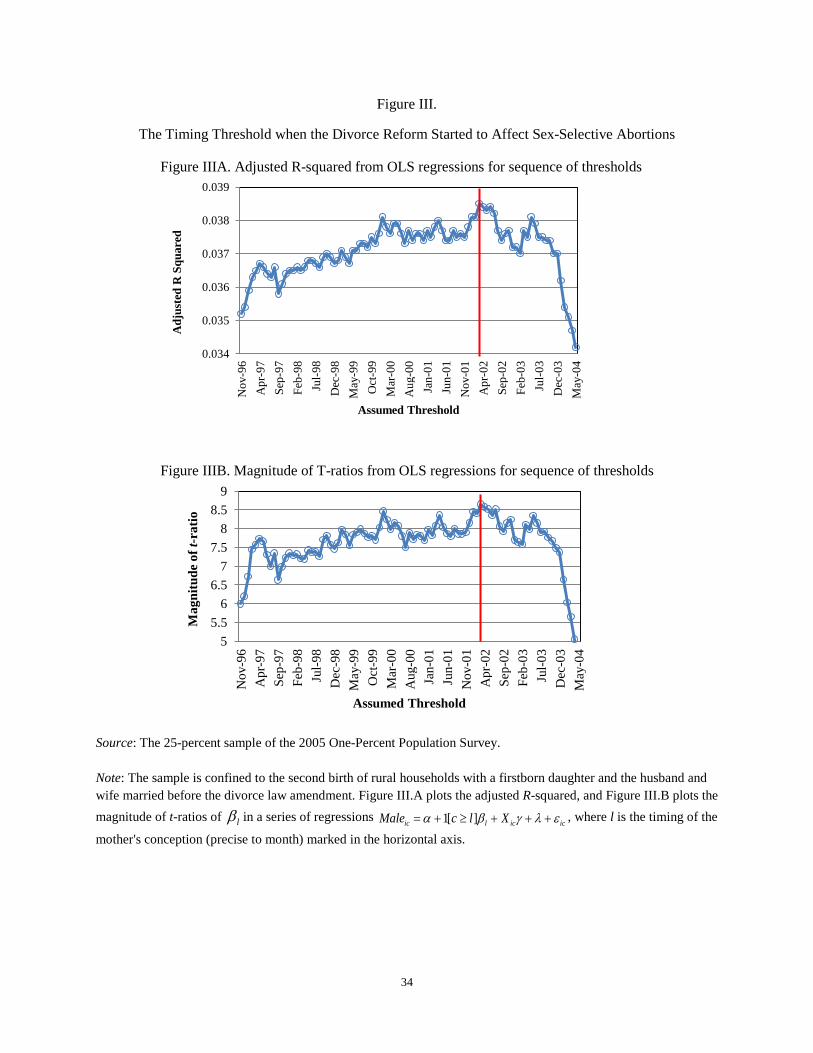
Source: The 25-percent sample of the 2005 One-Percent Population Survey. Note: The sample is confined to the second birth of rural households with a firstborn daughter and the husband and wife married before the divorce law amendment. Figure III.A plots the adjusted R-squared, and Figure III.B plots the magnitude of t-ratios of lβ in a series of regressions iciclic XlcMale ελγβα +++≥+= ][1 , where l is the timing of the
mother's conception (precise to month) marked in the horizontal axis.
0.034
0.035
0.036
0.037
0.038
0.039
Nov
-96
Apr
-97
Sep-
97
Feb-
98
Jul-9
8 D
ec-9
8 M
ay-9
9 O
ct-9
9 M
ar-0
0 A
ug-0
0 Ja
n-01
Ju
n-01
N
ov-0
1 A
pr-0
2 Se
p-02
Fe
b-03
Ju
l-03
Dec
-03
May
-04
Adj
uste
d R
Squ
ared
Assumed Threshold
5 5.5
6 6.5
7 7.5
8 8.5
9
Nov
-96
Apr
-97
Sep-
97
Feb-
98
Jul-9
8 D
ec-9
8 M
ay-9
9 O
ct-9
9 M
ar-0
0 A
ug-0
0 Ja
n-01
Ju
n-01
N
ov-0
1 A
pr-0
2 Se
p-02
Fe
b-03
Ju
l-03
Dec
-03
May
-04
Mag
nitu
de o
f t-r
atio
Assumed Threshold
35
Figure IV.
The Relationship between Timing of Mother's Conception and Propensity to Have a Second-born Son after a Firstborn Daughter
Source: The 25-percent sample of the 2005 One-Percent Population Survey.
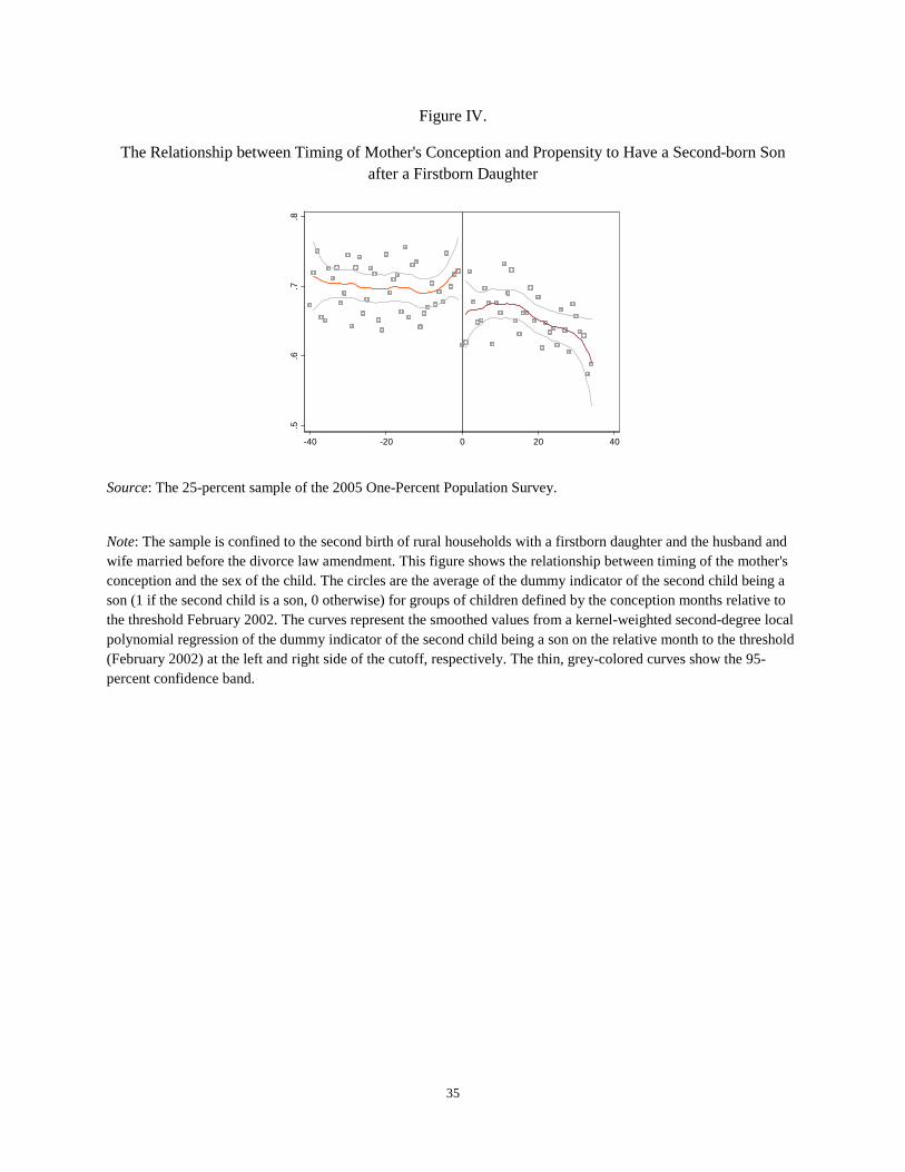
Note: The sample is confined to the second birth of rural households with a firstborn daughter and the husband and wife married before the divorce law amendment. This figure shows the relationship between timing of the mother's conception and the sex of the child. The circles are the average of the dummy indicator of the second child being a son (1 if the second child is a son, 0 otherwise) for groups of children defined by the conception months relative to the threshold February 2002. The curves represent the smoothed values from a kernel-weighted second-degree local polynomial regression of the dummy indicator of the second child being a son on the relative month to the threshold (February 2002) at the left and right side of the cutoff, respectively. The thin, grey-colored curves show the 95-percent confidence band.
.5.6
.7.8
-40 -20 0 20 40
36
Figure V.
The Relationship between Timing of Mother's Conception and the Spacing between a Firstborn Daughter and a Second-Born Child
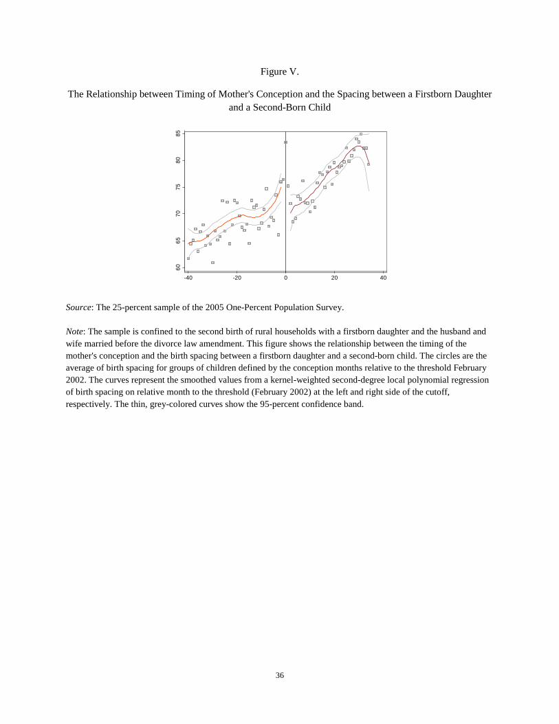
Source: The 25-percent sample of the 2005 One-Percent Population Survey. Note: The sample is confined to the second birth of rural households with a firstborn daughter and the husband and wife married before the divorce law amendment. This figure shows the relationship between the timing of the mother's conception and the birth spacing between a firstborn daughter and a second-born child. The circles are the average of birth spacing for groups of children defined by the conception months relative to the threshold February 2002. The curves represent the smoothed values from a kernel-weighted second-degree local polynomial regression of birth spacing on relative month to the threshold (February 2002) at the left and right side of the cutoff, respectively. The thin, grey-colored curves show the 95-percent confidence band.
6065
7075
8085
-40 -20 0 20 40
37
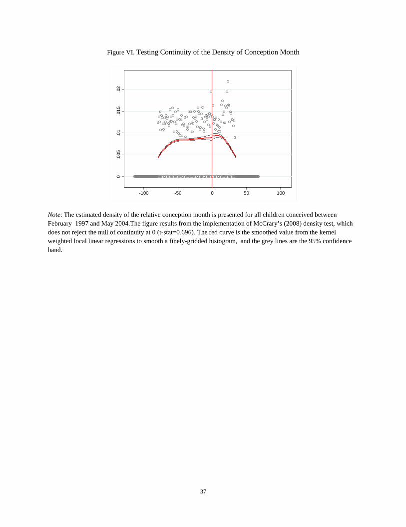
Figure VI. Testing Continuity of the Density of Conception Month
Note: The estimated density of the relative conception month is presented for all children conceived between February 1997 and May 2004.The figure results from the implementation of McCrary’s (2008) density test, which does not reject the null of continuity at 0 (t-stat=0.696). The red curve is the smoothed value from the kernel weighted local linear regressions to smooth a finely-gridded histogram, and the grey lines are the 95% confidence band.
0.0
05.0
1.0
15.0
2
-100 -50 0 50 100
38
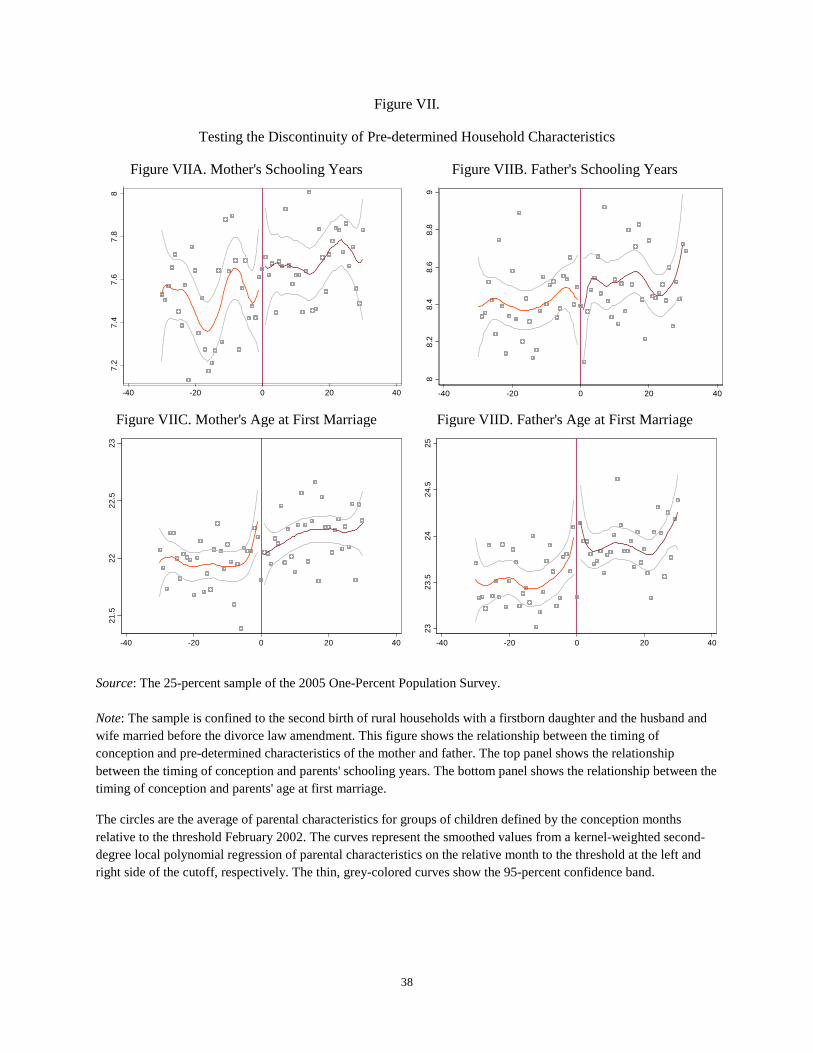
Figure VII.
Testing the Discontinuity of Pre-determined Household Characteristics
Figure VIIA. Mother's Schooling Years Figure VIIB. Father's Schooling Years
Figure VIIC. Mother's Age at First Marriage Figure VIID. Father's Age at First Marriage
Source: The 25-percent sample of the 2005 One-Percent Population Survey. Note: The sample is confined to the second birth of rural households with a firstborn daughter and the husband and wife married before the divorce law amendment. This figure shows the relationship between the timing of conception and pre-determined characteristics of the mother and father. The top panel shows the relationship between the timing of conception and parents' schooling years. The bottom panel shows the relationship between the timing of conception and parents' age at first marriage.
The circles are the average of parental characteristics for groups of children defined by the conception months relative to the threshold February 2002. The curves represent the smoothed values from a kernel-weighted second-degree local polynomial regression of parental characteristics on the relative month to the threshold at the left and right side of the cutoff, respectively. The thin, grey-colored curves show the 95-percent confidence band.
7.2
7.4
7.6
7.8
8
-40 -20 0 20 40
88.
28.
48.
68.
89
-40 -20 0 20 40
21.5
2222
.523
-40 -20 0 20 40
2323
.524
24.5
25
-40 -20 0 20 40
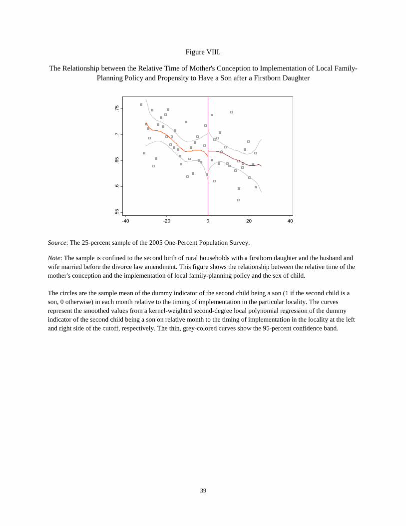
39
Figure VIII.
The Relationship between the Relative Time of Mother's Conception to Implementation of Local Family- Planning Policy and Propensity to Have a Son after a Firstborn Daughter
Source: The 25-percent sample of the 2005 One-Percent Population Survey. Note: The sample is confined to the second birth of rural households with a firstborn daughter and the husband and wife married before the divorce law amendment. This figure shows the relationship between the relative time of the mother's conception and the implementation of local family-planning policy and the sex of child. The circles are the sample mean of the dummy indicator of the second child being a son (1 if the second child is a son, 0 otherwise) in each month relative to the timing of implementation in the particular locality. The curves represent the smoothed values from a kernel-weighted second-degree local polynomial regression of the dummy indicator of the second child being a son on relative month to the timing of implementation in the locality at the left and right side of the cutoff, respectively. The thin, grey-colored curves show the 95-percent confidence band.
.55
.6.6
5.7
.75
-40 -20 0 20 40
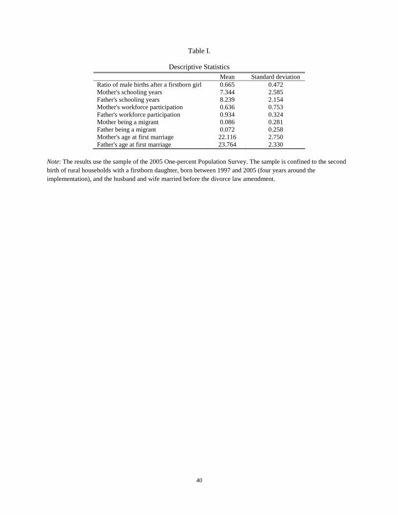
40
Table I.
Descriptive Statistics Mean Standard deviation
Ratio of male births after a firstborn girl 0.665 0.472 Mother's schooling years 7.344 2.585 Father's schooling years 8.239 2.154 Mother's workforce participation 0.636 0.753 Father's workforce participation 0.934 0.324 Mother being a migrant 0.086 0.281 Father being a migrant 0.072 0.258 Mother's age at first marriage 22.116 2.750 Father's age at first marriage 23.764 2.330
Note: The results use the sample of the 2005 One-percent Population Survey. The sample is confined to the second birth of rural households with a firstborn daughter, born between 1997 and 2005 (four years around the implementation), and the husband and wife married before the divorce law amendment.
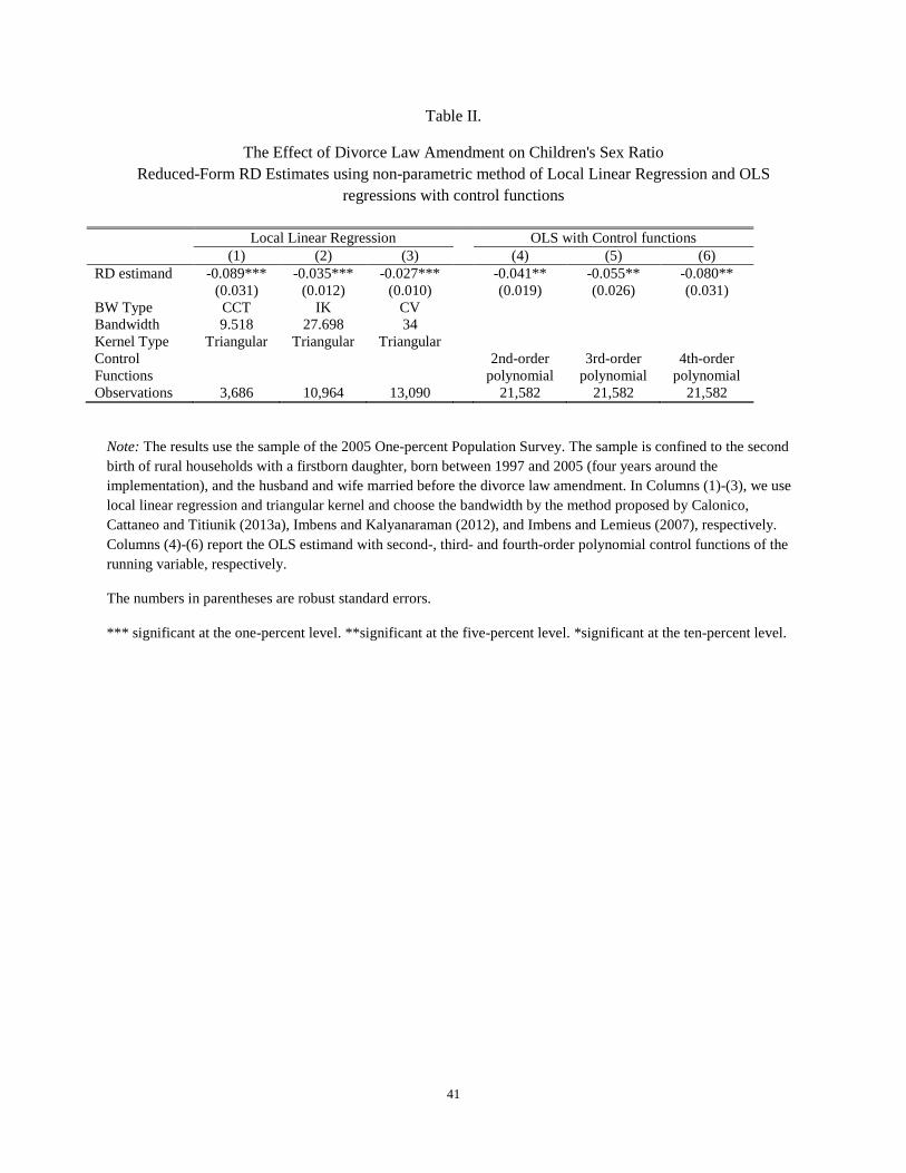
41
Table II.
The Effect of Divorce Law Amendment on Children's Sex Ratio Reduced-Form RD Estimates using non-parametric method of Local Linear Regression and OLS
regressions with control functions
Local Linear Regression OLS with Control functions (1) (2) (3) (4) (5) (6) RD estimand -0.089***
(0.031) -0.035***
(0.012) -0.027***
(0.010) -0.041**
(0.019) -0.055** (0.026)
-0.080** (0.031)
BW Type CCT IK CV Bandwidth 9.518 27.698 34 Kernel Type Triangular Triangular Triangular Control Functions
2nd-order polynomial
3rd-order polynomial
4th-order polynomial
Observations 3,686 10,964 13,090 21,582 21,582 21,582
Note: The results use the sample of the 2005 One-percent Population Survey. The sample is confined to the second birth of rural households with a firstborn daughter, born between 1997 and 2005 (four years around the implementation), and the husband and wife married before the divorce law amendment. In Columns (1)-(3), we use local linear regression and triangular kernel and choose the bandwidth by the method proposed by Calonico, Cattaneo and Titiunik (2013a), Imbens and Kalyanaraman (2012), and Imbens and Lemieus (2007), respectively. Columns (4)-(6) report the OLS estimand with second-, third- and fourth-order polynomial control functions of the running variable, respectively.
The numbers in parentheses are robust standard errors.
*** significant at the one-percent level. **significant at the five-percent level. *significant at the ten-percent level.

42
Table III.
The Effect of Divorce Law Amendment on Birth Spacing Reduced-Form RD Estimates using non-parametric method of Local Linear Regression and OLS
regressions with control functions
Local Linear Regression OLS with Control functions (1) (2) (3) (4) (5) (6) RD estimand -3.386*
(2.129) -2.669** (1.151)
-2.589** (1.277)
-2.303* (1.543)
-0.404 (2.124)
-0.617 (2.804)
BW Type CCT IK CV Bandwidth 11.970 43.781 33 Kernel Type Triangular Triangular Triangular Control Functions
2nd-order polynomial
3rd-order polynomial
4th-order polynomial
Observations 4,291 14,885 12,596 21,408 21,408 21,408
Note: The results use the sample of the 2005 One-percent Population Survey. The sample is confined to the second birth of rural households with a firstborn daughter, born between 1997 and 2005 (four years around the implementation), and the husband and wife married before the divorce law amendment. In Columns (1)-(3), we use local linear regression and triangular kernel and choose the bandwidth by the method proposed by Calonico, Cattaneo and Titiunik (2013a), Imbens and Kalyanaraman (2012), and Imbens and Lemieus (2007), respectively. Columns (4)-(6) report the OLS estimand with second-, third- and fourth-order polynomial control functions of the running variable, respectively.
The numbers in parentheses are robust standard errors.
*** significant at the one-percent level. **significant at the five-percent level. *significant at the ten-percent level.
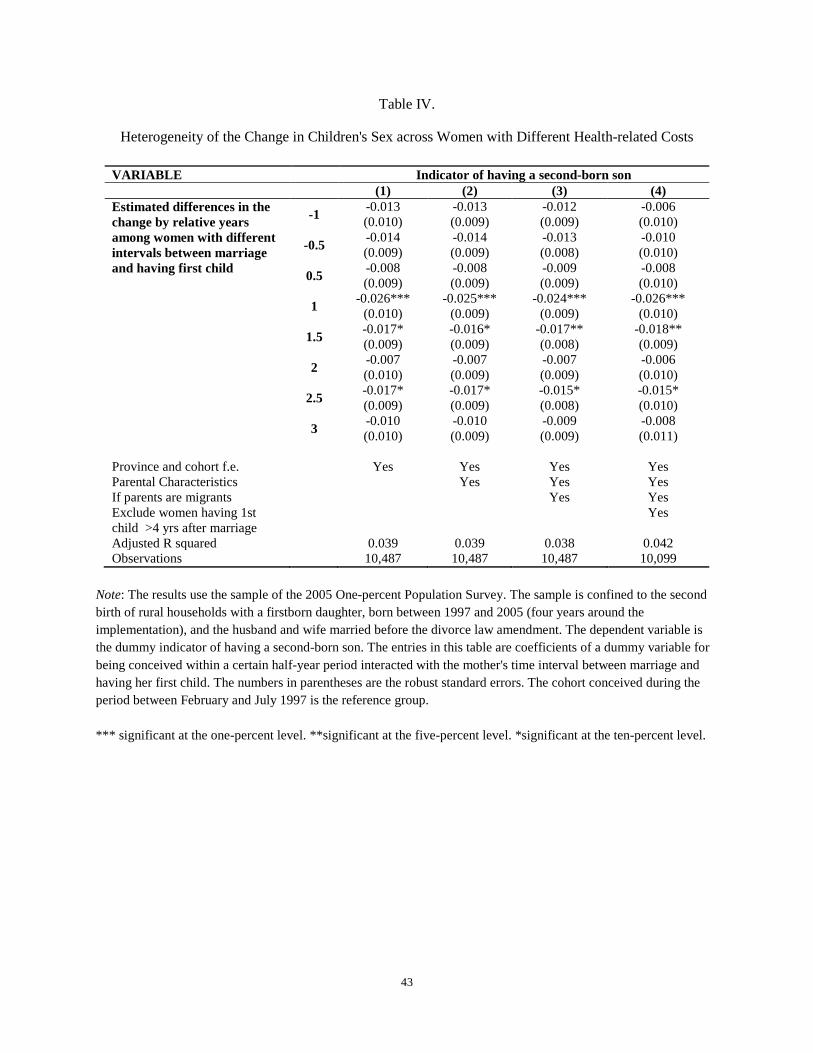
43
Table IV.
Heterogeneity of the Change in Children's Sex across Women with Different Health-related Costs
VARIABLE Indicator of having a second-born son (1) (2) (3) (4) Estimated differences in the change by relative years among women with different intervals between marriage and having first child
-1 -0.013 (0.010)
-0.013 (0.009)
-0.012 (0.009)
-0.006 (0.010)
-0.5 -0.014 (0.009)
-0.014 (0.009)
-0.013 (0.008)
-0.010 (0.010)
0.5 -0.008 (0.009)
-0.008 (0.009)
-0.009 (0.009)
-0.008 (0.010)
1 -0.026*** (0.010)
-0.025*** (0.009)
-0.024*** (0.009)
-0.026*** (0.010)
1.5 -0.017* (0.009)
-0.016* (0.009)
-0.017** (0.008)
-0.018** (0.009)
2 -0.007 (0.010)
-0.007 (0.009)
-0.007 (0.009)
-0.006 (0.010)
2.5 -0.017* (0.009)
-0.017* (0.009)
-0.015* (0.008)
-0.015* (0.010)
3 -0.010 (0.010)
-0.010 (0.009)
-0.009 (0.009)
-0.008 (0.011)
Province and cohort f.e. Yes Yes Yes Yes Parental Characteristics Yes Yes Yes If parents are migrants Yes Yes Exclude women having 1st child >4 yrs after marriage
Yes
Adjusted R squared 0.039 0.039 0.038 0.042 Observations 10,487 10,487 10,487 10,099
Note: The results use the sample of the 2005 One-percent Population Survey. The sample is confined to the second birth of rural households with a firstborn daughter, born between 1997 and 2005 (four years around the implementation), and the husband and wife married before the divorce law amendment. The dependent variable is the dummy indicator of having a second-born son. The entries in this table are coefficients of a dummy variable for being conceived within a certain half-year period interacted with the mother's time interval between marriage and having her first child. The numbers in parentheses are the robust standard errors. The cohort conceived during the period between February and July 1997 is the reference group. *** significant at the one-percent level. **significant at the five-percent level. *significant at the ten-percent level.
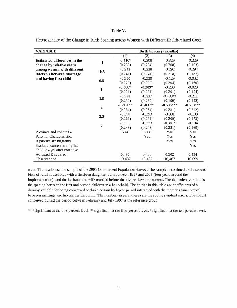
44
Table V.
Heterogeneity of the Change in Birth Spacing across Women with Different Health-related Costs
VARIABLE Birth Spacing (months) (1) (2) (3) (4) Estimated differences in the change by relative years among women with different intervals between marriage and having first child
-1 -0.410* (0.233)
-0.308 (0.234)
-0.329 (0.208)
-0.229 (0.163)
-0.5 -0.342 (0.241)
-0.328 (0.241)
-0.292 (0.218)
-0.294 (0.187)
0.5 -0.330 (0.229)
-0.330 (0.229)
-0.129 (0.204)
-0.032 (0.160)
1 -0.388* (0.231)
-0.389* (0.231)
-0.238 (0.201)
-0.023 (0.154)
1.5 -0.338 (0.230)
-0.337 (0.230)
-0.433** (0.199)
-0.211 (0.152)
2 -0.484** (0.234)
-0.486** (0.234)
-0.635*** (0.231)
-0.513*** (0.212)
2.5 -0.390 (0.261)
-0.393 (0.261)
-0.301 (0.209)
-0.108 (0.173)
3 -0.375 (0.248)
-0.373 (0.248)
-0.387* (0.221)
-0.104 (0.169)
Province and cohort f.e. Yes Yes Yes Yes Parental Characteristics Yes Yes Yes If parents are migrants Yes Yes Exclude women having 1st child >4 yrs after marriage
Yes
Adjusted R squared 0.496 0.486 0.502 0.494 Observations 10,487 10,487 10,487 10,099
Note: The results use the sample of the 2005 One-percent Population Survey. The sample is confined to the second birth of rural households with a firstborn daughter, born between 1997 and 2005 (four years around the implementation), and the husband and wife married before the divorce law amendment. The dependent variable is the spacing between the first and second children in a household. The entries in this table are coefficients of a dummy variable for being conceived within a certain half-year period interacted with the mother's time interval between marriage and having her first child. The numbers in parentheses are the robust standard errors. The cohort conceived during the period between February and July 1997 is the reference group. *** significant at the one-percent level. **significant at the five-percent level. *significant at the ten-percent level.
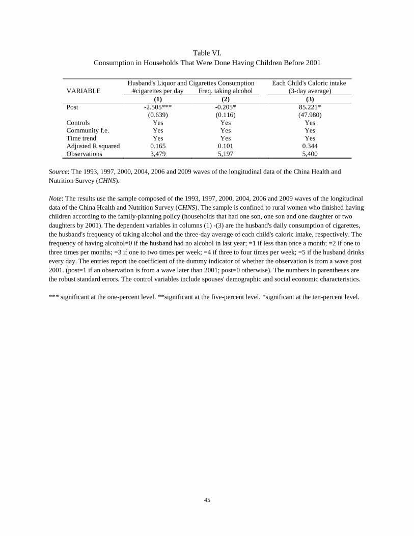
45
Table VI. Consumption in Households That Were Done Having Children Before 2001
Husband's Liquor and Cigarettes Consumption Each Child's Caloric intake VARIABLE #cigarettes per day Freq. taking alcohol (3-day average) (1) (2) (3) Post -2.505***
(0.639) -0.205* (0.116)
85.221* (47.980)
Controls Yes Yes Yes Community f.e. Yes Yes Yes Time trend Yes Yes Yes Adjusted R squared 0.165 0.101 0.344 Observations 3,479 5,197 5,400
Source: The 1993, 1997, 2000, 2004, 2006 and 2009 waves of the longitudinal data of the China Health and Nutrition Survey (CHNS). Note: The results use the sample composed of the 1993, 1997, 2000, 2004, 2006 and 2009 waves of the longitudinal data of the China Health and Nutrition Survey (CHNS). The sample is confined to rural women who finished having children according to the family-planning policy (households that had one son, one son and one daughter or two daughters by 2001). The dependent variables in columns (1) -(3) are the husband's daily consumption of cigarettes, the husband's frequency of taking alcohol and the three-day average of each child's caloric intake, respectively. The frequency of having alcohol=0 if the husband had no alcohol in last year; =1 if less than once a month; =2 if one to three times per months; =3 if one to two times per week; =4 if three to four times per week; =5 if the husband drinks every day. The entries report the coefficient of the dummy indicator of whether the observation is from a wave post 2001. (post=1 if an observation is from a wave later than 2001; post=0 otherwise). The numbers in parentheses are the robust standard errors. The control variables include spouses' demographic and social economic characteristics. *** significant at the one-percent level. **significant at the five-percent level. *significant at the ten-percent level.
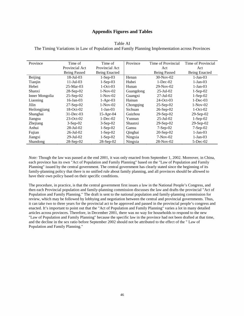
46
Appendix Figures and Tables
Table AI The Timing Variations in Law of Population and Family Planning Implementation across Provinces
Province Time of Provincial Act Being Passed
Time of Provincial Act Being Enacted
Province Time of Provincial Act
Being Passed
Time of Provincial Act
Being Enacted Beijing 18-Jul-03 1-Sep-03 Henan 30-Nov-02 1-Jan-03 Tianjin 11-Jul-03 1-Sep-03 Hubei 1-Dec-02 1-Jan-03 Hebei 25-Mar-03 1-Oct-03 Hunan 29-Nov-02 1-Jan-03 Shanxi 28-Sep-02 1-Nov-02 Guangdong 25-Jul-02 1-Sep-02 Inner Mongolia 25-Sep-02 1-Nov-02 Guangxi 27-Jul-02 1-Sep-02 Liaoning 16-Jan-03 1-Apr-03 Hainan 24-Oct-03 1-Dec-03 Jilin 27-Sep-02 1-Nov-02 Chongqing 25-Sep-02 1-Nov-02 Heilongjiang 18-Oct-02 1-Jan-03 Sichuan 26-Sep-02 1-Oct-02 Shanghai 31-Dec-03 15-Apr-04 Guizhou 29-Sep-02 29-Sep-02 Jiangsu 23-Oct-02 1-Dec-02 Yunnan 25-Jul-02 1-Sep-02 Zhejiang 3-Sep-02 3-Sep-02 Shaanxi 29-Sep-02 29-Sep-02 Anhui 28-Jul-02 1-Sep-02 Gansu 7-Sep-02 7-Sep-02 Fujian 26-Jul-02 1-Sep-02 Qinghai 20-Sep-02 1-Jan-03 Jiangxi 29-Jul-02 1-Sep-02 Ningxia 7-Nov-02 1-Jan-03 Shandong 28-Sep-02 28-Sep-02 Ningxia 28-Nov-02 5-Dec-02
Note: Though the law was passed at the end 2001, it was only enacted from September 1, 2002. Moreover, in China, each province has its own "Act of Population and Family Planning" based on the "Law of Population and Family Planning" issued by the central government. The central government has clearly stated since the beginning of its family-planning policy that there is no unified rule about family planning, and all provinces should be allowed to have their own policy based on their specific conditions. The procedure, in practice, is that the central government first issues a law in the National People’s Congress, and then each Provincial population and family-planning commission discusses the law and drafts the provincial "Act of Population and Family Planning." The draft is sent to the national population and family-planning commission for review, which may be followed by lobbying and negotiation between the central and provincial governments. Thus, it can take two to three years for the provincial act to be approved and passed in the provincial people’s congress and enacted. It’s important to point out that the "Act of Population and Family Planning" varies a lot in many detailed articles across provinces. Therefore, in December 2001, there was no way for households to respond to the new "Law of Population and Family Planning" because the specific law in the province had not been drafted at that time, and the decline in the sex ratio before September 2002 should not be attributed to the effect of the " Law of Population and Family Planning."