Do Bond Investors Price Tail Risk Exposures of

Financial Institutions?

Sudheer Chava∗ Rohan Ganduri† Vijay Yerramilli‡

March 2014

Abstract

We analyze whether bond investors price tail risk exposures of financial institutions us-

ing a comprehensive sample of bond issuances by U.S. financial institutions. Although

primary bond yield spreads increase with an institutions’ own tail risk (expected short-

fall), systematic tail risk (marginal expected shortfall) of the institution doesn’t affect

its yields. The relationship between yield spreads and tail risk is significantly weaker

for depository institutions, large institutions, government-sponsored entities, politically-

connected institutions, and in periods following large-scale bailouts of financial institu-

tions. Overall, our results suggest that implicit bailout guarantees of financial institu-

tions can exacerbate moral hazard in bond markets and weaken market discipline.

∗Scheller College of Business, Georgia Institute of Technology; 800 W. Peachtree St NW, Atlanta, GA30309; email: sudheer.chava@scheller.gatech.edu.†Scheller College of Business, Georgia Institute of Technology; 800 W. Peachtree St NW, Atlanta, GA

30309; email: rohan.ganduri@scheller.gatech.edu.‡C. T. Bauer College of Business, University of Houston; 240D Melcher Hall, University of Houston, Hous-

ton, TX 77204; email: vyerramilli@bauer.uh.edu. We are grateful to the 2013 GARP Risk ManagementProgram for financial support. We would like to thank Viral Acharya, Andy Winton, and seminar participantsat Scheller College of Business, Georgia Tech for helpful comments and suggestions.

1 Introduction

The experience of the recent financial crisis highlights two aspects of risk-taking by financial

institutions that reinforced each other in the run-up to the crisis and contributed to an increase

in systemic risk.1 First, executives at financial institutions have incentives to take on tail risks,

that is, risks that generate severe adverse consequences with small probability but, in return,

offer generous returns the rest of the time (Rajan (2005), Kashyap, Rajan, and Stein (2008),

Hoenig (2008) and Strahan (2013)). Second, institutions have incentives to herd with other

institutions in investment choices, thus increasing their exposure to systemically important

sectors, such as housing, because they expect to be bailed out in the event of a systemic crisis

(Farhi and Tirole (2011)).

Given the importance of the financial sector and the negative externality on the real

economy from a widespread failure of financial institutions, there is an increased focus on

how to contain tail risk exposures of financial institutions. One recurring idea in financial-

sector regulation is that regulators increase their reliance on “market discipline” in controlling

institutions’ risk exposures. However, market discipline can only be effective if investors price

the risk exposure of financial institutions. In this paper, we examine whether bond market

investors price the tail risk exposure of financial institutions in which they invest.

Financial institutions are highly-levered entities and their equity capital may not be ade-

quate to absorb the large losses that materialize when a tail event occurs. Given that bond-

holders hold uninsured liabilities that do not share in the upside from tail risk but may have

to absorb losses when the tail risk materializes, it is rational to expect that they will demand

higher yield spreads from institutions with higher tail risk exposures. This should be par-

ticularly true for investors in subordinated bonds, whose claims are junior to those of senior

bondholders.2 On the other hand, there are two reasons why bondholders may not price tail

1Systemic risk is the risk of widespread failure of financial institutions or the freezing up of capital markets(see Acharya, Pedersen, Philippon, and Richardson (2010) and Hansen (2011) for a more detailed discussion).

2In fact, Pillar III of the New Basel Capital Accord places special emphasis on market discipline throughsubordinated bonds, which are meant to act as loss-absorbing instruments.

1

risk exposures. Bondholders of systemically important financial institutions (SIFIs) may ra-

tionally anticipate a taxpayer-funded bailout of their institution in the event of a systemic

crisis, and thus, may not price the institution’s exposure to tail risk, especially systematic

tail risk. Alternatively, it may be that investors neglect low-probability nonsalient risks and

are caught unaware when the debt they had considered safe turns out to be risky (Bordalo,

Gennaioli, and Shleifer (2012) and Gennaioli, Shleifer, and Vishny (2012)).3

We test these hypotheses using a large sample of primary bond issuances by U.S. financial

institutions during the 1990 to 2010 period. We focus on the primary bond market because it

directly affects the cost of institutions’ debt capital. We measure an institution’s own tail risk

using expected shortfall (ES ), which measures its expected loss conditional on returns being

less than some α-quintile. Specifically, ES is defined as the negative of the average return on

the institution’s stock over the 5% worst return days for the institution over the year; i.e., ES

measures the institution’s loss in its own left tail. We capture the tail dependence between

the institution and the stock market using the marginal expected shortfall (MES ), which

measures the institution’s expected loss when the stock market is in its left tail (see Acharya,

Pedersen, Philippon, and Richardson (2010)). Specifically, MES is defined as the negative of

the average return on the institution’s stock over the 5% worst return days for the S&P 500

index over the year.4 Henceforth, we will refer to MES as the institution’s systematic tail

risk, to distinguish it from ES, which may also be driven by risk factors that are idiosyncratic

to the institution.

We first examine whether the yield spreads on new bond offerings at issuance (Yield

Spread) vary with the tail risk exposure of the financial institution issuing the bonds. As

expected, we find a robust positive relationship between Yield Spread and ES, which indicates

that the cost of debt capital is higher for institutions with a higher total tail risk. Interestingly,

3This view is supported by Jarrow, Li, Mesler, and van Deventer (2007) and Coval, Jurek, and Stafford(2009) who show that the sensitivities of structured products like CDOs to home prices were not taken intoaccount by rating agencies and investors alike.

4Acharya, Pedersen, Philippon, and Richardson (2010) show that MES is an important determinant of afinancial institution’s overall contribution to systemic risk, and that institutions with high MES before theonset of the financial crisis had worse stock returns during the crisis years, all else equal.

2

however, we fail to detect any significant relationship between Yield Spread and MES ; that

is, bond market investors seem to ignore an institution’s systematic tail risk. To alleviate

the concern that the effect of tail risk may be subsumed by a bond’s credit rating or an

institution’s size and leverage, we estimate our regression after omitting these important

controls, and obtain qualitatively similar results. To test the robustness of this result, we also

regress Yield Spread against other well-known risk measures, and arrive at a similar conclusion:

Yield Spread increases with the institution’s idiosyncratic risk (e.g., standard deviation of the

institution’s abnormal stock return) but does not vary with the institution’s systematic risk

(e.g., Beta).

We next explore how the relationship between yield spreads and tail risk varies with differ-

ent bond characteristics that can affect an institution’s default risk and the loss given default.

When we distinguish between senior and subordinate bonds, we find that, as expected, the

positive relationship between yield spreads and ES is significantly stronger for subordinated

bonds. However, the pricing of systematic tail risk MES does not vary between senior and

subordinated bonds. In fact, a more striking result is that the institutions’ MES is not priced

even in the case of subordinated bonds. We also find that, as expected, the positive relation-

ship between yield spreads and tail risk is stronger for bonds with poorer credit ratings.

Next, we examine how the pricing of tail risk varies with firm characteristics that may affect

bailout expectations. As Strahan (2013) highlights, if investors place a positive probability

that creditors would be protected in the event of failure, the prices of financial instruments

would be distorted - the greater the probability, the greater the distortion. Consistent with the

existence of too-big-to-fail (TBTF) subsidies for large financial institutions (e.g., see Acharya

et al. (2013)), we find that the relationship between yield spreads and total tail risk ES is

weaker for large financial institutions. However, there is no such variation in terms of the

pricing of MES, which is not priced regardless of the institution’s size. An interesting class of

institutions in our sample are the government-sponsored entities (GSEs) such as Fannie Mae

and Freddie Mac. Although bonds issued by GSEs carry no explicit government guarantee of

3

creditworthiness, there is a perception of an implicit guarantee because it is widely believed

that the government will not allow such important institutions to fail or default on their debt

(Strahan (2013)). Consistent with the existence of such an implicit guarantee, we find that

the relationship between yield spreads and tail risk measures is significantly weaker for GSEs.

We conduct several additional tests to further distinguish between the moral-hazard hy-

pothesis and the nonsalient-risks hypothesis. First, we estimate our regressions separately for

the following four categories of institutions: depository institutions, broker-dealers, insurance

companies, and other financial institutions. Institutions across these categories vary not only

in terms of their risk exposures and balance-sheet composition, but also in terms of implicit

bailout guarantees from the government. For instance, ever since the bailout of the Continen-

tal Illinois National Bank in 1984, the FDIC and other regulatory agencies have repeatedly

indicated that they consider large banks too-big-to-fail (TBTF) because their closure might

destabilize the financial system and impose a negative externality on the real economy. On

the other hand, there are no implicit guarantees for debt issued by insurance companies as

these are less likely to be considered systemically important. Thus, as per the moral-hazard

hypothesis, the relationship between bond yield spreads and tail risk should be weaker for

depository institutions compared with other types of financial institutions.

Consistent with this argument, we uncover striking differences in the pricing of tail risk

between depository institutions and other types of financial institutions. We find that neither

the total tail risk ES nor the systematic tail risk MES is priced in the case of bonds issued

by depository institutions, whereas both ES and MES are priced in the case of bonds issued

by broker-dealers and insurance companies. More strikingly, we find that ES and MES are

not priced even in the case of subordinated bonds issued by depository institutions. These

results cast serious doubt on the idea that market discipline can be used to control the tail

risk exposure of depository institutions.

Second, we examine how the relationship between yield spreads and tail risk varies based

on the political connectedness of financial institutions. The idea is to exploit political con-

4

nectedness as a source of cross-sectional variation in bailout expectations, because politically

connected institutions are more likely to receive government bailouts (Faccio et al. (2006)).

To test this idea, we hand-collect information on corporate lobbying expenditures by financial

institutions from the Center for Responsive Politics (CRP). Consistent with the moral-hazard

hypothesis, we find that the relationship between yield spreads and tail risk is significantly

weaker for politically-connected institutions compared with non-connected institutions.

Third, we examine how the relationship between yield spreads and tail risk varies in the

immediate aftermath of crisis events, such as the Long Term Capital Management (LTCM)

crisis and the recent financial crisis. The idea underlying this test is to exploit the time-series

variation in bailout expectations following the large-scale bailouts of troubled institutions

during these crises. Not surprisingly, we find an across-the-board increase in the cost of debt

for all financial institutions following a crisis event. However, consistent with the moral-hazard

hypothesis, the relationship between yield spreads and tail risk is significantly weaker in the

immediate aftermath of the LTCM crisis and the recent financial crisis. In sharp contrast,

we do not find any such patterns surrounding the dotcom crisis of 2001. This is interesting

because the dotcom crisis was confined to the technology sector and did not lead to bailouts of

financial institutions. This differential impact of the dotcom crash compared with the other

two crisis events suggests that our results are more likely driven by expectations of future

bailouts rather than a general neglect of nonsalient risks.

Our paper is closely related to and complements the results in a recent paper by Acharya

et al. (2013) that finds that secondary bond yield spreads of large financial institutions are

lower compared with other financial institutions even after controlling for their risk exposures.

They attribute this phenomenon to investor expectations of implicit state guarantees for

large institutions. Our paper differs from theirs in the following respects: First, we focus on

primary bond yield spreads that directly reflect the institutions’ cost of debt capital. Second,

our analysis is focused on the pricing of tail risk measures that are of particular concern to

bondholders, especially investors in subordinated bonds. Finally, we provide further support

5

for the moral-hazard hypothesis by showing that the pricing of tail risk is significantly weaker

for politically connected institutions compared with non-connected institutions. Overall, our

evidence points to moral hazard in the primary debt markets for financial institutions and

complements the secondary debt market evidence in Acharya et al. (2013).

Our paper is related to prior studies of bank market discipline that focus on whether

uninsured bank liabilities such as certificates of deposit (CDs) and subordinated notes and

debentures (SNDs) contain appropriate risk premia. The literature generally concludes that

CD rates paid by large money-center banks include significant default risk premia (e.g., see

Ellis and Flannery (1992), Hannan and Hanweck (1988), and Cargill (1989)). On the other

hand, the literature is divided with respect to the pricing of SNDs. Using a sample from

1983 and 1984, Avery, Belton, and Goldberg (1988) and Gorton and Santomero (1990) fail

to detect any relationship between SND pricing and balance sheet measures of bank risk.

However, examining a longer sample period, Flannery and Sorescu (1996) conclude that SND

prices become more sensitive to risk measurements as expectations of government-sponsored

bailouts decrease. The main difference between our study and this literature is that we focus

exclusively on the pricing of tail risk exposures of financial institutions. Similar to Avery,

Belton, and Goldberg (1988) and Gorton and Santomero (1990), we fail to find any evidence

that subordinated bondholders of depository institutions care more about tail risk than senior

bondholders. Also, similar to Flannery and Sorescu (1996), we find that the pricing of tail

risk changes with expectations of government bailouts.

Past research has highlighted the perverse impact of implicit bailout guarantees on risk-

taking behavior of financial institutions. This literature argues that expectations of future

systemic bailouts causes banks to correlate their risk exposure and take on high leverage

(Farhi and Tirole (2011)), incentivizes small banks to herd together with large banks and

increases the risk that many banks fail together (Acharya and Yorulmazer (2007)), and gener-

ally exacerbates the moral hazard of banks and bank managers (Bernardo, Talley, and Welch

(2011) and Ratnovski and DellAriccia (2012)). We contribute to this literature by highlight-

6

ing how implicit bailout guarantees also exacerbate the moral hazard of bond investors, thus

undermining bank market discipline. Our finding is also in line with a recent study by Kelly,

Lustig, and Van Nieuwerburgh (2011) that shows that a large amount of aggregate tail risk is

missing from the price of financial sector crash insurance (i.e., price of puts on the financial

sector index) during the recent financial crisis, which suggests that investors in the options

market are pricing in a collective government guarantee for the financial sector.

Our study has potential regulatory implications in favor of internal restructuring/bail-in

provisions, which lower the expectations of future government bailouts. In particular, it is

important that bondholders are made to share in any loss arising from the institution’s failure.

This is essential in restoring market discipline and ensuring that prices of uninsured liabilities

of financial institutions are in line with their risk exposures. Possibly recognizing these issues,

Mario Draghi, President of the European Central Bank (ECB), recently advocated that even

senior bondholders must share in the losses at the worst-hit savings banks in Spain. This

was in sharp contrast to the bailout of Irish banks in late 2010 in which unsecured senior

bondholders were paid in full using taxpayer money even though they had absolutely no form

of government guarantee.

The remainder of the paper is organized as follows. We describe our data sources and

construction of variables in Section 2, and provide descriptive statistics and preliminary results

in Section 3. We present our main empirical results in Section 4. We do additional tests in

Section 5 to distinguish between our competing hypotheses. Section 6 concludes the paper.

2 Data, Sample Construction, and Key Variables

Given the focus of our paper, our sample comprises only bonds issued by U.S. financial institu-

tions over the 1990 to 2010 period. Following Acharya et al. (2010), we classify U.S. financial

institutions into the following four groups based on SIC codes: depositories, which have a

2-digit SIC code of 60 (e.g., Bank of America, JP Morgan, Citigroup, etc.); broker-dealers,

7

which have a 4-digit SIC code of 6211 (e.g., Goldman Sachs, Morgan Stanley, etc.); insurance

companies, which have a 2-digit SIC code of either 63 or 64 (e.g., AIG, Metlife, Prudential,

etc.); and other financial institutions, which have a 2-digit SIC code of 61, 62, 65 or 67, and

consist of nonbank finance companies (e.g., American Express), real estate companies (e.g.,

CIT Group), and GSEs (e.g., FNMA and FHLM), etc. We include all financial institutions in

our sample regardless of their size. We have verified that our results are qualitatively similar

even if we confine our analysis to large institutions, defined as those with market capitalization

in excess of $5 billion dollars over the entire sample period. The names of these large U.S.

financial institutions are listed in Appendix A.

We obtain primary bond market data from Mergent’s Fixed Investment Securities Database

(FISD). FISD is a comprehensive database that provides issue details for over 140,000 cor-

porations, U.S. agencies, and U.S. Treasury debt securities.5 We restrict our sample to U.S.

domestic bonds and exclude yankee bonds, bonds issued via private placements, and issues

that are asset-backed or have credit-enhancement features. We also exclude preferred stocks,

mortgage-backed securities, trust-preferred capital, and convertible bonds.6 We include only

ratings issued by the top three NRSROs – Standard and Poor (S&P), Moody’s, and Fitch.

Our sample consists of both senior and subordinated bonds.7 We obtain firm-level control

variables from COMPUSTAT’s quarterly firm fundamentals file and merge this information

with the primary market data.

Our main dependent variable of interest is Yield Spread, which is the yield to maturity

(YTM) on the bond at issuance minus the YTM on a Treasury security with comparable

maturity. Another variable of interest is Rating, which measures the bond’s credit rating at

5FISD contains detailed information for each issue such as the issuer name, bond yields, bond yield spreadsover the closest benchmark treasury, maturity date, offering amount, bond types, optionality features, ratingdate, rating level, and the agency that rated the issue, etc. See Chava et al. (2010) for more details of theFISD database.

6Lehman Brothers and Morgan Stanley issued large number of equity-linked bonds in 2007 and 2008. Suchissues were dropped after a search based on the issue description field.

7FISD usually provides information regarding the seniority of the bond issue. In cases where the informationis not provided, we obtain the missing seniority information by matching the issue in FISD using its completeCUSIP with the corresponding issue in Moody’s Default Risk Database (DRS) and S&P’s CUSIP master file.Additionally, we also classify issues as senior or subordinated based on the issue description for bonds.

8

issuance. To obtain Rating, we first convert the credit ratings provided by S&P (Moody’s)

into an ordinal scale starting with 1 as AAA (Aaa), 2 as AA+ (Aa1), 3 as AA (Aa2), and so

on until 22, which denotes the default category. As Fitch provides three ratings for default,

we follow the existing literature and chose 23 instead of 22 for the default category, which

is the average of the three default ratings; i.e., DD. Because each bond issue may be rated

by multiple agencies, we compute Rating as the simple average of the ordinal rating assigned

by each rating agency. Note that by construction, a lower value for Rating denotes a better

credit quality at issuance.

We obtain stock price data from CRSP and use it to compute our risk measures. We

measure tail risk using expected shortfall (ES ), which is widely used within financial firms to

measure expected loss conditional on returns being less than some α-quintile. Its computation

involves identifying the 5% worst return days during the year for the firm’s stock (i.e., days on

which the return was lower than its fifth-percentile cutoff), and then computing the negative

of the average of the firm’s daily returns on these days. We measure systematic tail risk using

marginal expected shortfall (MES ), which measures the firm’s expected loss when the market

is in its left tail (see Acharya et al. (2010)). Specifically, MES is defined as the negative of

the average return on the firm’s stock over the 5% worst return days for the S&P500 index

over the year. As we show below, there is a high correlation between ES and MES in our

sample, which is not surprising: given the systemic importance of the financial sector, financial

institutions are more likely to experience a tail event when the market as a whole experiences

a tail event.

Apart from the tail risk measures, we also compute two commonly used measures of risk:

Aggregate Risk, which is a measure of the total firm-specific risk and defined as the standard

deviation of the firm’s daily excess return (i.e., daily return on a firm’s stock in excess of the

daily return on the S&P500 index) over the year; and Beta, which is a measure of systematic

risk, and is obtained by estimating the market model Rit = αi + βiRmt + εit using daily

returns over the year. We use a rolling yearly window to compute the risk measures, so that

9

for each quarter, risk measures are computed using the information from the preceding four

quarters. For example, the risk measures pertaining to quarter from April 2007 to June 2007

are computed using the stock and S&P returns over the one-year period from April 2006 to

March 2007.

3 Descriptive Statistics and Preliminary Results

3.1 Summary Statistics

We provide a year-wise summary of bond offerings by financial institutions during the 1990 to

2010 period in Table I. As can be seen, there is a great deal of variation in total annual bond

issuances by number over our sample period, with the 1992–1995 period being the most active

in terms of number of bonds issued. However, although there were fewer issues in the latter

half of the sample period, the median offering amount in the second half of the sample period

is significantly higher than in the first half. Therefore, examining the total dollar amount

issued each year, we find that the later half of the sample period has a larger dollar amount of

bonds issued even though there are a fewer number of total issues in this period. The majority

of the sample consists of senior bonds, with subordinated bonds making up only 18% of total

issuances by number. A little more than half of the bonds in our sample have a maturity of

less than 10 years and about half have a redeemable feature.

We provide the mean and median values (in parentheses) of the key variables by institution

type in Panel B of Table I. Examining firm characteristics, we see that broker-dealers have

the highest leverage, whereas insurance companies have the lowest leverage. On average,

depository and broker-dealer institutions are also larger (higher log(assets)) and better rated

(lower Rating) than insurance firms. Consistent with Acharya et al. (2010), depository

institutions have lower aggregate risk and lower tail risk (both ES and MES ), whereas broker-

dealers have the highest level of systematic risk (Beta), tail risk (ES ), and systematic tail risk

(MES ) mainly due to the nature of their business. Other financial institutions account for

10

half of the total bond issuances in our sample; out of these, GSEs account for about 40%.

Depository institutions account for about a quarter of the total bond issuances by number,

whereas broker-dealers and insurance firms together account for another quarter. However, as

can be seen from the mean and median offering sizes, the bond offerings by broker-dealers and

depository institutions are much larger in size compared with those of insurance companies

and other financial institutions. Depository institutions are the main issuers of subordinated

debt, which accounts for around 40% of their bond offerings. This is mainly due to regulatory

reasons. As per the Basel Capital Accord, subordinated debt is among the three types of

eligible loss-absorbing instruments that banks are required to issue at regular intervals in

order to facilitate market discipline.

3.2 Correlations

We provide univariate correlations between our key variables in Table II. Not surprisingly,

total tail risk (ES ) and systematic tail risk (MES ) are highly correlated. This suggests that,

given the systemic importance of the financial sector, financial institutions are more likely

to experience a tail event when the market as a whole experiences a tail event. Therefore,

in our subsequent multivariate analysis, we are careful to only include either ES or MES

as an independent variable. We also note the high correlation between ES and Aggregate

Risk, which suggests that riskier institutions also have higher tail risk. Similarly, the high

correlation between Beta and MES suggests that institutions with high overall systematic

risk also have higher systematic tail risk.

We find that Yield Spread is positively correlated with the tail risk measures (ES, MES )

and Aggregate Risk. We must, however, interpret this with caution because these are univariate

correlations that do not control for other important institutional characteristics. In particu-

lar, Yield Spread is negatively correlated with Size and Leverage, which are two important

characteristics that are positively correlated with tail risk. In the case of rating assignments,

we find that Rating is positively correlated with ES and Aggregate Risk, suggesting that in-

11

stitutions with higher tail risk and higher total risk are assigned worse ratings. On the other

hand, Rating is uncorrelated with MES. As with the yield spreads, we find that Rating is

highly negatively correlated with Size and Leverage, suggesting that large and highly levered

financial institutions are assigned better ratings.

We now proceed to multivariate analysis in which we examine the relationship between

Yield Spread and tail risk after controlling for differences in size, leverage, and other risk

characteristics across institutions.

4 Empirical Results

4.1 Bond Yield Spreads and Tail Risk

We begin our empirical analysis by examining whether investors in the primary bond markets

price the tail risk exposures of the financial institution issuing the bonds. To test this, we

estimate the following OLS regression model:

Yield Spreadift = α + β ∗ Tail Riskf,t + γ ∗Xf,t−1 + ρ ∗Xi + Y earFE + InstTypeFE.

In the above equation, we use subscript ‘i’ to denote the bond, subscript ‘f’ to denote the

issuer firm, and subscript ‘t’ to denote the quarter of issuance. Each observation in the

regression sample corresponds to a primary bond issue. The main dependent variable of

interest is the bond’s Yield Spread at issuance. The main independent variable of interest is

Tail Risk, which we measure using either ES or MES. We control the regression for important

firm characteristics (Xf ), issue characteristics (Xi), and macroeconomic variables that may

affect Yield Spread. All the variables are defined in the Appendix. The firm characteristics

that we control for are Size, Profitability, market leverage (Leverage), and book leverage

(LongTermDebt Assets). The issue characteristics that we control for are the bond’s Rating,

issue size, maturity, and indicator variables to identify subordinated debt, callable bonds, and

12

agency debt. We also include year fixed effects in all specifications, and control for Term

Spread, which is defined as the yield spread between 10-year and 1-year Treasury bonds.

We begin by estimating regression (4.1) on all financial institutions in our sample pooled

together, but include institution-type fixed effects to control for differences between depository

institutions, broker-dealers, insurance companies, and other financial institutions. The results

of our estimation are presented in Table III. The standard errors reported in parentheses are

robust to heteroskedasticity, and are clustered at the level of the institution.

The main independent variable of interest is ES in column (1) and MES in column (2).

As we mentioned previously, we do not include ES and MES simultaneously to avoid multi-

collinearity. The positive and significant coefficient on ES in column (1) indicates that yield

spreads at issuance are higher for bonds issued by institutions with high tail risk. A one stan-

dard deviation increase in ES increases the primary bond issuance yield by 18 basis points.

However, the coefficient on MES in column (2) is statistically insignificant, and is also much

smaller in magnitude than the coefficient on ES in column (1). Thus, it appears from the

results in column (1) and (2) that primary bond market investors care about the institution’s

total tail risk, but not its systematic component of tail risk.

The coefficients on the control variables in columns (1) and (2) are broadly as expected.

The positive coefficients on Rating and Maturity indicate that yield spreads are higher for

lower rated bonds and longer maturity bonds, whereas the negative coefficient on Log(Issue

Size) indicates that yield spreads are lower for larger issues. Examining firm characteristics,

we find that yield spreads are higher for institutions with higher leverage. However, controlling

for issue size, the size of the institution has no effect on yield spreads.

One possible reason for the lack of a significant association between Yield Spread and MES

is that we may be over-controlling our regressions. That is, it is possible that the impact of the

tail risk measures is being subsumed by Size, Leverage, Rating, and other firm-level factors,

which we showed to be significantly correlated with the risk measures. To alleviate this

concern, we repeat our tests from (1) and (2) after omitting all firm-level controls and the

13

bond’s credit rating. The results are reported in columns (3) and (4). As can be seen by

comparing columns (1) and (3), the coefficient on ES does become stronger after we omit

firm-level controls and rating from the regression specification, suggesting that the omitted

controls are somewhat subsuming the effect of ES. However, the coefficient on MES continues

to be insignificant and actually decreases in magnitude after omission of the controls.

To summarize, the results in Table III suggest that primary bond market investors care

about the institution’s total tail risk, but not its systematic component of tail risk.

4.2 Bond Yield Spreads and Other Risk Measures

A potential concern with our interpretation of the results in Table III is that MES may not

be a good measure of the systematic component of tail risk. We do not believe that this

is a valid concern because Acharya, Pedersen, Philippon, and Richardson (2010) show that

MES is an important determinant of a financial institution’s overall contribution to systemic

risk, and that institutions with high MES before the onset of the financial crisis had worse

stock returns during the crisis years, all else equal. Nonetheless, to alleviate this concern, we

examine how primary bond yield spreads vary with other well-known risk measures, such as

Volatility and Beta.

The results of our estimation are presented in Table IV. Apart from the fact that we

employ different risk measures, the empirical specification and control variables in columns

(1) through (3) are exactly the same as that of column (1) of Table III. That is, we control for

the full set of firm-level and issue characteristics, and include year fixed effects and institution-

type fixed effects. However, to conserve space, we do not report the coefficients on the control

variables.

The risk measures of interest in columns (1) and (2) are Volatility and Beta, respectively.

Recall that Volatility is a measure of the institution’s aggregate risk, whereas Beta is widely

used as a measure of systematic risk. Consistent with our results in Table III, we find that

primary bond market investors price the institution’s aggregate risk (positive and significant

14

coefficient on Volatility) but do not price its systematic risk (insignificant coefficient on Beta).

As we noted in Table II, ES and MES are highly correlated. To isolate the idiosyncratic

component of tail risk, we construct a new risk measure, ES idio, by orthogonalizing ES with

respect to MES.8 We then estimate regression (4.1) after including both ES idio and MES as

independent variables. As can be seen from column (3), the coefficient on ES idio is positive

and significant whereas the coefficient on MES is insignificant. Moreover, the coefficient on

ES idio appears to be larger than the coefficient on ES in column (1) of Table III. Thus, it

appears that primary bond market investors only price the idiosyncratic component of the

institution’s tail risk.

As in Table III, we repeat the estimations in columns (1) through (3) after omitting firm-

level characteristics and credit rating as control variables, just to make sure that these control

variables are not subsuming the effect of the risk variables. As can be seen from columns (4)

through (6), our qualitative results hold even after we omit these control variables. Moreover,

consistent with our findings in Table III, the coefficients on Volatility and ES idio become

stronger after the omission of the control variables, whereas the coefficient on Beta becomes

significantly weaker.

Note that the results in Tables III and IV are more consistent with the moral-hazard hy-

pothesis than the nonsalient-risks hypothesis. As per the nonsalient-risks hypothesis, yield

spreads should not respond to either the idiosyncratic or the systematic component of tail

risk. However, we find that although bond yield spreads do not respond to the systematic

component of tail risk (MES ), they do increase with the total tail risk (ES ) and the idiosyn-

cratic component of tail risk (ES idio). On the other hand, given that bailouts are more likely

in the event of a systemic failure, the fact that investors only ignore MES is consistent with

the moral-hazard hypothesis.

8Formally, we obtain ES idio by adding the constant and the residual from the regression of ES on MES.We conduct the orthogonalization separately for each institution type because the sensitivity of ES to MEScan vary across depositories, broker-dealers, insurance companies, and other financial institutions.

15

4.3 Variation of Results with Bond Characteristics

In this section, we examine how our baseline results on the association between Yield Spread

and risk measures vary with key bond characteristics, such as seniority, maturity, and rating.

The results of our analysis are in Table V.

In columns (1) and (2) of Table V, we examine how the pricing of tail risk varies between

senior and subordinated bonds. Absent government bailout, the loss given default should be

significantly higher for subordinated bonds. Hence, it is logical to expect that the positive

association between Yield Spread and tail risk measures should be stronger for subordinated

bonds. To test this, we define the dummy variable d Sub to identify subordinated bonds, and

estimate regression (4.1) after including d Sub and its interaction with the tail risk measures

as additional regressors. The empirical specification and control variables are exactly the same

as in columns (1) and (2) of Table III, although we suppress the coefficients on the control

variables in order to conserve space. The positive and significant coefficient on d Sub×ES in

column (1) indicates that the association between tail risk and yield spreads is indeed stronger

for subordinated bonds. However, the insignificant coefficient on d Sub×MES indicates that

there is no incremental effect of MES on yield spreads for subordinated bonds over senior

bonds. A more striking finding is that the sum of the coefficients on MES and d Sub×MES

is also statistically insignificant, which suggests that MES is not priced even in the case of

subordinated bonds issued by financial institutions.

In columns (3) and (4), we examine how our baseline results vary with the bond’s credit

quality at issuance. Intuitively, we expect our results to be stronger for bonds with lower

credit ratings. To test this, we define the dummy variable d LowGrade to identify bonds with

an S&P credit rating of “A” or worse at issuance (i.e., Rating≥ 5), and interact this with the

tail risk measures.9 The positive coefficients on the interaction terms d LowGrade×ES and

d LowGrade×MES indicate that the effect of tail risk on yield spreads is indeed stronger for

9High-grade bonds (defined as those with credit rating of AAA or AA) constitute roughly 33% of oursample, medium-grade bonds (defined as those with credit rating between A and BBB) constitute 63% of oursample, and speculative-grade bonds (i.e., credit rating worse than BBB) constitute the remaining 4%.

16

low grade bonds. These results are inconsistent with the nonsalient-risks hypothesis as yield

spreads respond to both the idiosyncratic and systematic component of tail risk.

In columns (5) and (6), we examine whether the effect of tail risk on yield spreads is

stronger for longer maturity bonds. There are two reasons to expect that the effect should

be stronger for longer maturity bonds. First, there is more uncertainty in the long run than

in the short run. Second, given that financial institutions rely heavily on short-term debt,

long-term bondholders are also exposed to the risk that the institution may not be able to

rollover or refinance its short-term debt (“rollover risk”). To test this, we define the dummy

variable d LongMat to identify bonds with stated maturity of 10 years or more. We then

estimate our baseline regressions after including d LongMat and its interaction with the tail

risk measures as additional regressors. As can be seen from the insignificant coefficients on

d LongMat×ES and d LongMat×MES, we fail to detect any incremental effect of tail risk on

primary yield spreads for longer maturity bonds. Moreover, the sum of the coefficients on

MES and d LongMat×MES in column (4) is also statistically insignificant, which suggests

that MES is not priced for long maturity bonds.

4.4 Variation of Results with Firm Characteristics

Next, we examine how our baseline results on the association between Yield Spread and tail

risk measures vary with important firm characteristics, such as size, leverage, and implicit

bailout expectations. The results of our analysis are in Table VI.

We begin with the effect of firm size. As per the moral-hazard hypothesis, the relationship

between Yield Spread and tail risk should be weaker for large institutions, which are more

likely to be considered systemically important and qualify for implicit too-big-to-fail guar-

antees. To test this, we define the dummy variable d Large to identify firms that are larger

than the median size by the book value of assets in the universe of all the financial firms

in COMPUSTAT.10 We then estimate our baseline regressions after including d Large and

10This classification yields 144 small firms and 160 large firms. However, the large firms contribute to more

17

its interactions with tail risk measures as additional regressors. The negative and significant

coefficient on d Large×ES in column (1) indicates that the incremental effect of ES on Yield

Spread is significantly weaker for large institutions. However, the sum of coefficients on ES

and d Large×ES is still positive and significant, which suggests that yield spreads increase

with total tail risk even for large financial institutions. On the other hand, the coefficients

on MES and d Large×MES in column (2), as well as the sum of these coefficients are all

statistically insignificant. This indicates that yield spreads do not vary with MES regardless

of the institution’s size.

In columns (3) and (4), we examine if our results vary with the level of the institution’s

leverage. As with size, we define the dummy variable d HighLeverage to identify institutions

whose market leverage exceeds the median leverage in the universe of all the financial firms

in COMPUSTAT. As expected, the positive and significant coefficient on d Leverage signifies

that firms with higher leverage have higher bond yield spreads, all else equal. However, we fail

to find any incremental effect of tail risk on yield spreads for institutions with high leverage.

An interesting class of institutions in our sample are the GSEs such as Fannie Mae and

Freddie Mac. Although bonds issued by GSEs carry no explicit government guarantee of

creditworthiness, there is a perception of an implicit guarantee because it is widely believed

that the government will not allow such important institutions to fail or default on their debt.11

Hence, as per the moral-hazard hypothesis, we should also expect the relationship between

Yield Spread and tail risk measures to be weaker for GSEs. We examine this in columns (5) and

(6) where we interact the tail risk measures with d Agency, a dummy variable that identifies

GSEs. The strong negative and significant coefficients on d Agency×ES and d Agency×MES

indicate that the effect of tail risk exposure on yield spreads is indeed much weaker for bonds

issued by GSEs.

As a further robustness check, in unreported results, we also compare financial firms and

than three-quarters of the issuance sample while the remainder comes from the smaller firms.11According to estimates by the Congressional Budget Office and the Treasury Department in 1997, GSEs

saved about $2 billion per year in funding costs because of this implicit guarantee.

18

industrial firms by employing the nearest-neighborhood (NN) matching technique (see Abadie,

Drukker, Herr, and Imbens (2004)) to match debt issued by financial firms to debt issued by

non-financials (industrial firms). We conduct an exact matching on the subordination status,

callability feature, and year of origination, and then use the NN matching on the remaining

controls in the bond yield spread regression model, namely, Rating, LogAssets, Profitability,

LongTermDebt Assets, Leverage, LogIssueSize, and Maturity.12 To ensure that our results are

not sensitive to the sample of matched counterfactuals, we match each bond offering by a

financial institution (treated sample) with three bond offerings by non-financial firms (control

sample). We find that investors do not price the systematic tail risk exposures of financial

institutions for their senior or their subordinated debt issuances. Overall, our matched sample

analysis gives further credence to the moral-hazard hypothesis that investors choose to ignore

tail risks for certain types of firms based on their expectation of future bailouts.

5 Additional Robustness Tests

As we noted in the introduction, there are two potential reasons why primary bond market

investors may not price an institution’s tail risk. It may be that bond market investors are

subject to moral hazard because, given the systemic importance of the financial sector, they

rationally anticipate taxpayer-funded bailouts in the event of large losses. Alternatively, it may

be that investors neglect low-probability nonsalient risks, in general, and are caught unaware

when the debt that they had considered safe turns out to be risky (Gennaioli, Shleifer, and

Vishny (2012)). In this section, we conduct additional tests aimed at distinguishing between

these competing hypotheses.

12Optimal matching resulted in 100% matching on the subordinated and callable dummy, and 91% onoffering year of the bond. As the optimal matching on offering year is not exact, we include year fixed effectsin our regressions.

19

5.1 Variation of Results Across Institution Types

One way to distinguish between the moral-hazard hypothesis and the nonsalient-risk hy-

pothesis is to examine how the pricing of tail risk varies across different types of financial

institutions. Certain types of financial institutions, such as depositories and GSEs, are more

likely to be considered systemically important because the failure of such institutions imposes

a large negative externality on the real economy. Such institutions are also more likely to

receive government bailouts if a negative event materializes. Thus, as per the moral-hazard

hypothesis, the relationship between bond yield spreads and tail risk should be weaker for

depository institutions compared with other types of financial institutions.

To test this idea, we now estimate regression (4.1) separately for bonds issued by each

institution type. The results of our estimation are presented in Panel A of Table VII. We esti-

mate the regressions separately on the subsamples of bonds issued by depository institutions

(columns (1) and (2)), broker-dealers (columns (3) and (4)), insurance companies (columns (5)

and (6)), and other financial institutions (columns (7) and (8)). We control these regressions

for the full set of firm and bond characteristics as in Table III, and also include year fixed

effects. However, to conserve space, we do not report the coefficients on the control variables.

As can be seen, the results in Panel A highlight a striking difference in the pricing of tail

risk between bonds issued by depository institutions and bonds issued by all other types of

financial institutions. The insignificant coefficients on ES and MES in columns (1) and (2)

indicate that the cost of debt for depository institutions does not vary with their exposure

to tail risk. On the other hand, we find a positive and significant association between Yield

Spread and tail risk measures for all other institution types, except for the category of other

financial institutions for which the coefficient on MES is positive but statistically insignificant.

The lack of significance on MES in column (8) may be driven by bonds issued by GSEs, which

are included in the category of other financial institutions. As we showed in Panel B of Table

VI, the relationship between bond yield spreads and tail risk is significantly weaker in case of

bonds issued by GSEs.

20

Our results in Panel A cast doubt on the idea that primary bond markets can provide

effective market discipline to depository institutions. One particular category of bonds that

bank regulators and supervisors rely on to enhance market discipline are subordinated bonds,

which are meant to act as loss-bearing instruments and are thus treated as part of regulatory

capital. As we noted in the discussion following Table I, depository institutions are by far

the largest issuers of subordinated bonds. In Panel B of Table VII, we separately examine

whether the pricing of tail risk varies between subordinated and senior bonds for depository

institutions (in columns (1) and (2)) and for all other types of financial institutions (in columns

(3) and (4)).

The positive and significant coefficient on d Sub×ES in column (1) indicates that in the

case of bonds issued by depository institutions, the relationship between Yield Spread and ES

is indeed stronger for subordinated bonds. However, the coefficient on ES is itself negative,

although not statistically significant. Moreover, the sum of coefficients on ES and d Sub×ES

is insignificant, which indicates that tail risk is not priced even in the case of subordinated

bonds issued by depository institutions. In column (2), we find that the coefficients on MES

and d Sub×MES, as well as the sum of these coefficients, are all statistically insignificant.

That is, systematic tail risk MES is not priced either for senior or subordinated bonds issued

by depository institutions.

Turning to the non-depository institutions, we can see that the coefficients on d Sub×ES in

column (3) and d Sub×MES in column (4) are both positive but are not statistically significant

at the conventional 10% level (the t−statistics of 1.61 and 1.49, respectively, are lower than the

cutoff value of 1.652). However, the coefficient on ES as well as the sum of coefficients on ES

and d Sub×ES in column (3) are both statistically significant, which indicates that total tail

risk is priced for both senior and subordinated bonds issued by non-depository institutions.

The same is true for systematic tail risk MES in column (4).

Overall, the results in Table VII indicate that the pricing of tail risk in the primary bond

market varies between depository institutions and non-depository institutions. The result that

21

neither ES nor MES is priced for bonds issued by depository institutions is consistent with

the moral-hazard hypothesis, because depository institutions are more likely to be considered

systemically important and benefit from implicit government guarantees. In unreported tests,

we verify that the qualitative results in Table VII are robust to the exclusion of firm-level

characteristics and credit rating as control variables; that is, we verify that the effect of tail

risk is not being subsumed by Size, Leverage, and Rating of depository institutions.

5.2 Political Connectedness and the Pricing of Tail Risk

In this section, we focus on cross-sectional variation in bailout expectations across financial

institutions. One such source of cross-sectional variation is the political connectedness of

financial institutions. If politically connected institutions are more likely to receive government

bailouts, then we expect the relationship between bond yield spreads and tail risk measures

to be weaker for better connected institutions.

We measure political connectedness using information on lobbying expenditures by fi-

nancial institutions obtained from the Center for Responsive Politics (CRP), which com-

piles data from lobbying disclosure reports filed with the Secretary of the Senate’s Office of

Public Records (SOPR).13 This data is available from 1998 through the most recent quar-

ter. We hand-match lobbying records with our data set by firm name and broad industry

classification. We measure political connectedness using two variables: a dummy variable

d PoliticalConnection, which identifies financial institutions that have ever lobbied the gov-

ernment; and Log(Lobby Expenditure), which is the natural logarithm of the amount of total

lobbying expenditure by the institution since the data became available in 1998.

As per our definition of d PoliticalConnection, 53% of the institutions in our sample are

politically connected, and include large institutions that were bailed out during the recent

13This data is also publicly available for download on SOPR’s website. As per the lobbying disclosure actof 1995, firms that hire lobbyists are required to provide a good-faith estimate rounded to the nearest $20,000of all lobbying-related expenditures in each six-month period. An organization that spends less than $10,000in any six-month period does not have to state its expenditures. In those cases, the Center treats the figureas zero.

22

financial crisis; e.g., Bear Stearns, AIG, Citigroup, Merrill Lynch, Bank of America, JP Mor-

gan, CIT Group, Freddie Mac, and Fannie Mae among others. The average lobbying amount

per year for our sample of firms is close to $1.8 million. Depositories on average have the

highest lobbying amount per year, as well as the highest percentage of politically connected

firms, followed by broker-dealers. In general, there seems to be a positive correlation between

our measures of political connectedness and bailout probability (Faccio et al. (2006)). A

simple correlation analysis shows that our measures of political connectedness are positively

correlated with firm assets and leverage, which implies that larger institutions lobby the gov-

ernment more. Similarly, the correlation between Yield Spread and our political connections

measures are negatively correlated, which indicates that politically connected firms seem to

enjoy a lower cost of capital.

To test whether the pricing of tail risk varies with the institutions’ political connectedness,

we estimate regression (4.1) after including our measures of political connectedness and their

interactions with the tail risk measures as additional regressors. We can estimate this regres-

sion only for the 1998 to 2010 period as the data on lobbying expenditures is available only

after 1998. The results of our analysis are presented in Table VIII. The empirical specification

and control variables are exactly the same as in Table III although we suppress the coefficients

on control variables in order to conserve space.

The negative and significant coefficients on d PoliticalConnection×ES and Log(Lobby Ex-

penditure)×ES in columns (1) and (3), respectively, indicate that the relationship between

Yield Spread and tail risk is indeed weaker for politically connected institutions. On the

other hand, although the coefficients on d PoliticalConnection×MES and Log(Lobby Expen-

diture)×MES in columns (2) and (4), respectively, are negative, they are not statistically

significant. Hence, we cannot conclude that the pricing of systematic tail risk varies between

politically-connected and non-connected financial institutions.

If the entire financial sector is expected to be bailed out during a crisis, then the pricing of

a firm’s systematic tail risk MES may vary less with its political connectedness during such

23

crisis periods. However, unconditionally, regardless of the state of the economy, one can expect

the probability of bailout to be higher for politically connected firms. As a robustness check,

we present a subsample analysis in columns (5) to (8) for the non-crisis period extending from

2001:Q2 to 2008:Q2, which spans a crisis-free period immediately after the LTCM and dotcom

crises and immediately prior to the recent financial crisis. In line with our expectation, not only

do we find that MES is mispriced for politically connected firms, but the severity of mispricing

of ES has also increased. Overall, this analysis confirms that the pricing relevance of tail risks

decreases with an increase in bailout probability as measured by political connectedness. This

is again consistent with the moral-hazard hypothesis.

Overall, the results in Table VIII provide more evidence in support of the moral-hazard

hypothesis by highlighting that primary bond market investors are less likely to price the tail

risk exposures of politically-connected institutions.

5.3 Pricing of Tail Risk Around Crisis Periods

In the previous section, we used political connectedness to identify the cross-sectional variation

in bailout expectations across firms. Another way to distinguish between the moral-hazard

hypothesis and the nonsalient-risks hypothesis is to examine how the association between

Yield Spread and the tail risk measures varies around crisis periods. In general, a crisis can

affect the pricing of tail risk in two ways. In the absence of bailout expectations, a crisis may

serve as a reminder of the existence of tail risks, and thus strengthen the relationship between

Yield Spread and the tail risk. However, if the crisis triggers large-scale bailouts of troubled

institutions, that may weaken the relationship between Yield Spread and the tail risk.

To better understand these effects, we focus on three crisis events that occurred during

our sample period: the failure and bailout of LTCM in August 1998, the dotcom crash of

March 2000, and the recent financial crisis in March 2008. Note that unlike the dotcom crash,

which was largely confined to the technology sector, the LTCM crisis and the recent financial

crisis adversely affected the financial sector and triggered government bailouts of troubled

24

institutions. We exploit this key difference to understand the extent to which our results are

being driven by changes in expectations of future bailouts. For each of these crisis events, we

construct a sample of bond issuances by all financial institutions that occurred in a two-year

(i.e., eight calendar quarters) window around the crisis event, and divide this into pre-crisis

and post-crisis windows of four calendars quarters each.14 We then compare how the pricing

of tail risk varies between the pre-crisis and post-crisis samples.

The results of our analysis are summarized in Table IX. In columns (1) and (2), we examine

the effect of the LTCM crisis that occurred during August and September of 1998. The LTCM

bailout was announced on September 23, 1998 when 14 financial institutions agreed to a $3.6

billion recapitalization under the supervision of the Federal Reserve. Accordingly, we use the

sample of bonds issued during the two-year period from 1997:Q4 to 1999:Q3 surrounding this

crisis event; the sample consists of 154 bond offerings. In this sample, we define the dummy

variable d LTCM to identify bonds issued between 1998:Q4 and 1999:Q3, that is, after the

LTCM bailout was announced. We then estimate regression (4.1) after including d LTCM and

its interactions with the tail risk variables as additional regressors. The empirical specification

and control variables are otherwise the same as in Table III, but with one important difference:

we exclude the year dummies, and instead use the specific crisis dummy to understand how

the pricing of tail risk changed pre- and post-crisis. We suppress the coefficients on the control

variables in order to conserve space.

The positive and significant coefficients on d LTCM in columns (1) and (2) indicate that

primary bond yield spreads of financial firms increased significantly in the immediate after-

math of the LTCM crisis. However, the negative and significant coefficients on d LTCM×ES

and d LTCM×MES in columns (1) and (2), respectively, indicate that the relationship be-

tween Yield Spread and tail risk was significantly weaker in the immediate aftermath of the

LTCM crisis. Moreover, the sum of the coefficients on ES and d LTCM×ES in column (1) is

14Choosing a two-year window around the crisis provides a reasonable sample size for our analysis withoutintroducing other confounding events, thus allowing for cleaner interpretation of results. We must note that itis not feasible to conduct these tests separately for each institution type as the sample size for each institutiontype would be very small. Hence, we conduct these tests for all financial institutions pooled together, butinclude institution-type fixed effects in the regression specification.

25

insignificant, and so is the sum of the coefficients on MES and d LTCM×MES in column (2).

These indicate that tail risk was not priced at all in the immediate aftermath of the LTCM

crisis.

We examine the effect of the recent financial crisis in columns (3) and (4). The main

events of the financial crisis occurred during mid-September to early October of 2008.15 Ac-

cordingly, to understand the impact of the financial crisis, we use the sample of bonds issued

during the two-year period from 2007:Q4 to 2009:Q3. In this sample, we use the dummy

variable d FinCrisis to identify bonds issued between 2008:4Q and 2009:Q3, which denotes

the post-crisis period. As can be seen from columns (3) and (4), the impact of the financial

crisis was very similar to that of the LTCM crisis: although there was an across-the-board

increase in primary bond yield spreads for all financial institutions following the crisis (posi-

tive coefficient on d FinCrisis), the relationship between yield spreads and tail risk was also

significantly weaker after the crisis as evidenced by the negative and significant coefficients on

d FinCrisis×ES and d FinCrisis×MES.

Finally, in columns (5) and (6), we study the effect of the dotcom crisis, which was triggered

by the collapse of the NASDAQ-100 Index on March 10, 2000. Accordingly, we use the

sample of bonds issued in the two-year period from 1999:Q2 to 2001:Q1. In this sample, the

dummy variable d Dotcom identifies bonds issued between the period 2000:Q2 and 2001:Q1,

the period right after the dotcom bubble burst on March 10, 2000. As with the LTCM crisis

and the financial crisis of 2008, we find that there was an across-the-board increase in primary

bond yield spreads of financial institutions in the immediate aftermath of the dotcom crisis

(positive and significant coefficient on d DotCom). However, in stark contrast to the other two

crises, the coefficients on d DotCom×ES and d DotCom×MES are statistically insignificant,

which suggests that there was no difference in the pricing of tail risk in the primary bond

markets in the immediate aftermath of the dotcom crisis. This could be due to the fact that

15The collapse of Lehman Brothers and the collapse and bailout of AIG occurred on September 15 and 16,2008, triggering widespread panic and a liquidity crisis that required the intervention of the U.S. governmentand the Federal Reserve. In the next few weeks, other financial institutions including Merrill Lynch, FannieMae, Freddie Mac, Washington Mutual, Wachovia, and Citigroup were either acquired under duress, or weresubject to government takeover.

26

the dotcom crash did not change bond market investors’ expectations of future bailouts of

financial institutions.

Overall, the evidence in Table IX lends more support to the moral-hazard hypothesis over

the nonsalient-risks hypothesis.

5.4 Do Rating Agencies Account for Tail Risk Exposures?

Investors may rely on rating agencies to price tail risk, as rating agencies specialize in de-

termining creditworthiness of firms. For example, a rating agency may be better positioned

to judge the quality of loans and other non-traded assets on a bank’s balance sheet. Rating

agencies also have access to a firm’s private information as they were exempt from the Fair

Disclosure Regulation (Reg FD) during our sample period. If rating agencies are also subject

to the aforementioned bailout moral hazard problem then they may not price tail risk. Bond

investors, who may rely on rating agencies to price tail risks, will consequently not price it

too. On the other hand rating agencies may price tail risk and investors might rationally

choose to ignore them. To investigate this issue we run an ordered probit model with Rating

as the dependent variable, and ES and MES as the key independent variables of interest. We

include all the control variables in equation (4.1) except of course Rating itself. The results

of our estimation are presented in Panel A of Table X.

In columns (1) and (2), we estimate the regression separately on the subsample of bonds

issued by depository institutions. Although we find a positive association between Rating and

total tail risk (ES ), we fail to find any association between Rating and systematic tail risk

(MES ). Interestingly, while rating agencies appear to price ES, investors seem to ignore it as

shown in Table VII. In columns (3) and (4), we estimate the regression separately on the

subsample of bonds issued by broker-dealers. In this subsample, we fail to find any significant

association between Rating and either tail risk or systematic tail risk. In contrast, even though

rating agencies seem to ignore the tail risk exposures of broker-dealers, primary bond market

investors as shown in Table VII seem well aware of these risks and do price them. When

27

we estimate the regression on bonds issued by insurance companies (columns (5) and (6))

and other financial institutions (columns (7) and (8)), we find a positive association between

Rating and both tail risk measures, which is particularly strong for bonds issued by insurance

companies.

Next, we examine how the association between Rating and the tail risk measures varies

with bonds’ seniority status. As in the previous section, we repeat our regression in Panel A

after including the interaction terms d Sub×ES and d Sub×MES, where d Sub is an indicator

variable that identifies subordinated bonds. The results of the estimation are presented in

Panel B. The positive and significant coefficient on d Sub indicates that subordinated bonds

are assigned lower ratings, all else equal, which is to be expected because the loss given default

should be higher for these bonds. However, surprisingly, there is no adverse incremental effect

of tail risk on the credit ratings of subordinated bonds. As can be seen, the coefficients on

d Sub×ES and d Sub×MES are mostly insignificant; in fact, we find a negative and significant

coefficient on d Sub×ES in column (1). In a separate row, we also report the statistical

significance on the sum of coefficients on the tail risk measure and its interaction term with

the d Sub dummy. Overall, these coefficients are positive and significant for depositories

whereas they are insignificant for the rest of the financial firms suggesting that rating agencies

account for tail risk for subordinated debt issued by depositories although not incrementally

over senior bonds.

To summarize, the results in Table X highlight interesting differences in how credit rating

agencies rate new bond issuances by different types of financial institutions compared with

investors. In particular, rating agencies do not seem to account for tail risk exposures of

broker-dealers and the systematic tail risk exposure of depository institutions. More strik-

ingly, although subordinated bonds are assigned lower credit ratings, there is no additional

adverse impact of the institution’s tail risk on the credit ratings assigned to subordinated

bonds. Again, to ensure we are not over-controlling our regressions, we repeat all of our tests

from Panels A and B after omitting these firm-level factors as controls. The results of these

28

robustness tests are however not reported and our qualitative results from Panels A and B are

unchanged when we omit these additional controls. The only noticeable difference is that the

coefficient on MES is significantly lower for these repeat tests of Panels A and B and all of the

sum of coefficients on the tail risk measure and its interaction term with the d Sub dummy

are small and statistically insignificant. Overall, the ordered probit rating regression results

indicate that it is not the investors’ reliance on rating agencies that leads to the mispricing of

tail risk.

6 Conclusion

In the aftermath of the recent financial crisis, there is an increased focus on containing tail risk

and systematic risk exposure of financial institutions. One recurring idea in financial sector

regulation is for regulators to increase their reliance on “market discipline” in controlling

institutions’ risk exposure. However, market discipline is effective only if investors price the

risk exposure of financial institutions. In the recent U.S. subprime financial crisis, large-

scale government interventions were enacted, which included bailouts designed to prevent

the financial industry from a potential system-wide breakdown. However, a consequence

of implied government guarantees and bailouts for financial institutions is a weakening of

market discipline. Investors can be subject to moral hazard and may not rationally price an

institution’s exposure to tail risks.

In this paper, we use a large sample of bond issuances by U.S. financial institutions dur-

ing the 1990 to 2010 period to examine whether bond market investors price the tail risk

exposure of financial institutions. We find that primary bond yield spreads increase with

institutions’ own tail risk (expected shortfall) but do not respond to their systematic tail risk

(marginal expected shortfall), even in the case of subordinated bonds. When we distinguish

between different types of financial institutions, we find a striking result that primary bond

yield spreads of depository institutions do not respond to tail risk for either senior bonds or

subordinated bonds. On the other hand, primary bond yield spreads of broker-dealers and

29

insurance companies respond to both total tail risk and systematic tail risk.

There are two potential explanations for why bond market investors may neglect tail risk

exposure of financial institutions. It may be that bond market investors are subject to moral

hazard because they rationally expect to be bailed out by the government if a negative tail

event materializes. Alternatively, it may be that investors neglect low-probability nonsalient

risks are are caught unaware when the assets that they had considered to be safe turn out to

be risky. Consistent with the moral-hazard hypothesis, we find that systematic tail risk is not

priced in situations where ex-ante bailout expectations are higher: that is, for depositories

and government-sponsored entities (GSEs), large institutions, and politically connected firms.

Moreover, bond investors’ concern for tail risk seems to have weakened in the immediate

aftermath of financial crises (such as LTCM and the recent financial crisis) that involved

government bailouts of financial institutions.

Overall, our results point to moral hazard in the primary bond markets due to implicit

bailout guarantees and cast doubt on the idea that market discipline can be effective in

controlling the tail risk exposures of depository institutions.

30

References

Abadie, A., D. Drukker, J. L. Herr, and G. W. Imbens (2004). Implementing matchingestimators for average treatment effects in stata. Stata journal 4, 290–311.

Acharya, V. and T. Yorulmazer (2007). Too many to fail: An analysis of time-inconsistencyin bank closure policies. Journal of Fixed Income 16, 1–31.

Acharya, V. V., D. Anginer, and A. J. Warburton (2013). The End of Market Discipline?investor Expectations of Implicit State Guarantees. NYU Working Paper.

Acharya, V. V., L. H. Pedersen, T. Philippon, and M. Richardson (2010, November). Mea-suring systemic risk. NYU Working Paper.

Avery, R., T. Belton, and M. Goldberg (1988). Market discipline in regulating bank risk: Newevidence from the capital markets. 20, 597–610.

Bernardo, A., E. Talley, and I. Welch (2011). A model of optimal government bailouts.Working Paper.

Bordalo, P., N. Gennaioli, and A. Shleifer (2012). Salience theory of choice under risk. Quar-terly Journal of Economics 127 (3), 1243–1285.

Cargill, T. F. (1989). CAMEL Ratings and the CD Market. Journal of Financial ServicesResearch, 347–358.

Chava, S., P. Kumar, and A. Warga (2010). Managerial agency and bond covenants. Reviewof Financial Studies 23 (3), 1120–1148.

Coval, J. D., J. W. Jurek, and E. Stafford (2009). The economics of structured finance. TheJournal of Economic Perspectives 23 (1), 3–26.

Ellis, D. M. and M. J. Flannery (1992). Does the debt market assess large banks’ risk? Journalof Monetary Economics 30, 481–502.

Faccio, M., R. W. Masulis, and J. J. McConnell (2006). Political Connections and CorporateBailouts. Journal of Finance 61, 2597–2635.

Farhi, E. and J. Tirole (2011). Collective moral hazard, maturity mismatch and systemicbailouts. American Economic Review 102 (1), 60–93.

Flannery, M. J. and S. M. Sorescu (1996). Evidence of bank market discipline in subordinateddebenture yields: 1983–1991. Journal of Finance 51, 1347–1377.

Gennaioli, N., A. Shleifer, and R. Vishny (2012). Neglected risks, financial innovation, andfinancial fragility. Journal of Financial Economics 104, 452–468.

Gorton, G. and A. Santomero (1990). Market discipline and bank subordinated debt. 22,119–128.

31

Hannan, T. H. and G. A. Hanweck (1988). Bank insolvency risk and the market for largecertificates of deposit. 20, 203–212.

Hansen, L. P. (2011). Challenges in identifying and measuring systemic risk. NBER WorkingPaper.

Hoenig, T. M. (2008, March). Perspectives on the recent financial market turmoil. Remarksat the 2008 Institute of International Finance Membership Meeting, Rio de Janeiro, Brazil,March 5.

Jarrow, R., L. Li, M. Mesler, and D. van Deventer (2007). CDO valuation: Fact and fiction.The Definitive Guide to CDOs, Risk Publications .

Kashyap, A. K., R. G. Rajan, and J. C. Stein (2008). Rethinking capital regulation. NBERworking paper.

Kelly, B. T., H. Lustig, and S. Van Nieuwerburgh (2011). Too-systemic-to-fail: What optionmarkets imply about sector-wide government guarantees. NBER Working Paper.

Rajan, R. G. (2005). Has financial development made the world riskier? Proceedings of theJackson Hole Conference organized by the Kansas City Fed.

Ratnovski, L. and G. DellAriccia (2012). Bailouts, contagion, and moral hazard. WorkingPaper.

Strahan, P. E. (2013). Too big to fail: Causes, consequences, and policy responses. AnnualReview of Financial Economics 5 (1), 43–61.

32

App

endix

A:

Nam

es

of

the

sam

ple

U.S

financi

al

inst

ituti

ons.

Th

eta

ble

dis

pla

ys

the

nam

esof

the

U.S

.fi

nan

cial

firm

sin

asu

bsa

mp

leh

avin

ga

mark

etca

pit

ali

zati

on

of

gre

ate

rth

an$5

bil

lion

.T

he

firm

sar

eca

tegori

zed

into

4gro

up

s:D

eposi

tori

es(2

-dig

itS

ICco

de=

60);

Bro

ker-

Dea

lers

(4-

dig

itS

ICco

de=

6211

);In

sura

nce

(2-d

igit

SIC

cod

e=60

&64);

Oth

er(2

-dig

itS

ICco

de=

61,

62

(exce

pt

6211),

65,

67)

Dep

osi

tory

Bro

ker

-Dea

lers

Insu

ran

ceO

ther

BANK

OF

AMERIC

ACORP

BEAR

STEARNSCOMPANIE

SIN

CAFLAC

INC

AMERIC

AN

CAPIT

AL

LTD

BANK

OF

NEW

YORK

MELLON

CORP

BLACKROCK

INC

AXA

FIN

ANCIA

LIN

CAMERIC

AN

EXPRESSCO

BANK

ONE

CORP

DEAN

WIT

TER

DISCOVER

&CO

AETNA

INC

AMERIP

RISE

FIN

ANCIA

LIN

CBANKAMERIC

ACORP

ETRADE

FIN

ANCIA

LCORP

ALLSTATE

CORP

AVIS

BUDGET

GROUP

INC

BANKERSTRUST

CORP

FRANKLIN

RESOURCESIN

CAMBAC

FIN

ANCIA

LGROUP

INC

CIT

GROUP

INC

CIT

IGROUP

INC

GOLDMAN

SACHSGROUP

INC

AMERIC

AN

INTERNATIO

NAL

GROUP

INC

CME

GROUP

INC

COMERIC

AIN

CLEHMAN

BROTHERSHOLDIN

GSIN

CBERKSHIR

EHATHAWAY

INC

DEL

CAPIT

AL

ONE

FIN

ANCIA

LCORP

FIR

STAR

CORP

NEW

WIS

MERRIL

LLYNCH

&CO

INC

CNO

FIN

ANCIA

LGROUP

INC

CIG

NA

CORP

FLEETBOSTON

FIN

ANCIA

LCORP

MORGAN

STANLEY

DEAN

WIT

TER

&CO

CIG

NA

CORP

CREDIT

SUISSE

FIR

ST

BOSTON

USA

GOLDEN

WEST

FIN

ANCIA

LCORP

SCHWAB

CHARLESCORP

CIN

CIN

NATIFIN

ANCIA

LCORP

EQUIT

YRESID

ENTIA

LJP

MORGAN

CHASE

&CO

COVENTRY

HEALTH

CARE

INC

FEDERAL

HOME

LOAN

MORTGAGE

CORP

M&

TBANK

CORP

GENW

ORTH

FIN

ANCIA

LIN

CFEDERAL

NATIO

NAL

MORTGAGE

ASSN

MARSHALL

&IL

SLEY

CORP

HANCOCK

JOHN

FIN

ANCIA

LSVCSIN

CFRANKLIN

RESOURCESIN

CNATIO

NAL

CIT

YCORP

HARTFORD

FIN

ANCIA

LSVCSGRP

INC

GOLDEN

WEST

FIN

ANCIA

LCORP

NORTHERN

TRUST

CORP

HUMANA

INC

HEALTH

CARE

REIT

INC

REGIO

NSFIN

ANCIA

LCORP

MBIA

INC

ISTAR

FIN

ANCIA

LIN

CSOVEREIG

NBANCORP

INC

MGIC

INVESTMENT

CORP

WIS

JANUSCAP

GROUP

INC

STATE

STREET

CORP

MARSH

&MCLENNAN

COSIN

CKIM

CO

REALTY

CORP

SUNAMERIC

AIN

CMETLIF

EIN

CNYSE

EURONEXT

SUNTRUST

BANKSIN

CNATIO

NW

IDE

FIN

ANCIA

LSERVIC

ESIN

NATIO

NAL

CIT

YCORP

SYNOVUSFIN

ANCIA

LCORP

PRIN

CIP

AL

FIN

ANCIA

LGROUP

INC

PAIN

EW

EBBER

GROUP

INC

UNIO

NPLANTERSCORP

PROVID

ENT

COMPANIE

SIN

CPROLOGIS

WACHOVIA

CORP

PRUDENTIA

LFIN

ANCIA

LIN

CSLM

CORP

WASHIN

GTON

MUTUAL

INC

TORCHMARK

CORP

TD

AMERIT

RADE

HOLDIN

GCORP

WELLSFARGO

&CO

TRAVELERSCOMPANIE

SIN

CW

ESTERN

UNIO

NCO

UNIT

EDHEALTH

GROUP

INC

UNUM

GROUP

WELLPOIN

THEALTH

NETW

RKSIN

C

33

Appendix B : Bond yields regression variables.

• Total debt = long-term debt + short-term debt

• Market value of assets = (stock price × shares outstanding) at bond issuance + Bookvalue of debt

• Term spread = yield spread between the 10- and 1-year treasury bonds

• Profitability = operating income after depreciation ÷ sales

• Long-term debt to total assets (book leverage) = long-term debt ÷ book value of totalassets

• Leverage (market leverage) = market value of assets ÷ market value of equity

34

Table

I:Sum

mary

stati

stic

sof

bond

sam

ple

.

The

table

dis

pla

ys

the

sum

mar

yst

atis

tics

ofth

esa

mple

ofse

nio

ran

dsu

bor

din

ated

corp

orat

eb

onds

issu

edby

U.S

.finan

cial

firm

s(1

-dig

itSIC

code=

6)duri

ng

the

per

iod

from

1990

to20

10.

We

rest

rict

our

sam

ple

toU

.S.

dom

esti

cb

onds

and

excl

ude

yanke

eb

onds,

bon

ds

issu

edvia

pri

vate

pla

cem

ents

,is

sues

whic

har

eas

set-

bac

ked

orhav

ecr

edit

-enhan

cem

ent

feat

ure

s.In

addit

ion

we

excl

ude

pre

ferr

edst

ock

s,m

ortg

age

bac

ked

secu

riti

es,

trust

pre

ferr

edca

pit

alan

dco

nve

rtib

leb

onds.

Pan

elA

dis

pla

ys

the

sum

mar

yst

atis

tics

year

-wis

e.T

he

num

ber

sfo

rSub

ordin

ated

,M

aturi

ty,

and

Cal

lable

feat

ure

are

expre

ssed

asa

per

centa

geof

the

tota

lsa

mple

.In

addit

ion,

Pan

elB

dis

pla

ys

the

sum

mar

yst

atis

tics

by

firm

-typ

efo

rou

rri

skm

easu

res,

bon

d-l

evel

vari

able

san

dfirm

-le

vel

vari

able

s.O

ur

tail

risk

mea

sure

sar

edefi

ned

as:

ES

:th

eneg

ativ

eof

the

aver

age

ofth

efirm

’sdai

lyre

turn

son

5%w

orst

retu

rnday

sduri

ng

the

cale

ndar

year

for

the

firm

;M

ES

:th

eneg

ativ

eof

the

aver

age

firm

’sdai

lyre

turn

on5%

wor

stre

turn

day

sof

the

mar

ket

(S&

P50

0in

stea

dof

for

the

firm

)duri

ng

the

cale

ndar

year

;E

Sidio

:is

the

resi

dual

plu

sco

nst

ant

up

onre

gres

sing

ES

onM

ES

separ

atel

yfo

rea

chfirm

-typ

e.O

ther

risk

mea

sure

sar

eSD

abnre

t:is

the

stan

dar

ddev

iati

onof

dai

ly“e

xce

ss”

retu

rnfo

rth

efirm

(i.e

.,firm

’sdai

lyre

turn

min

us

dai

lyre

turn

onS&

P50

0)ov

erth

eca

lendar

year

;B

eta

:is

the

esti

mat

eof

the

coeffi

cien

tup

onre

gres

sing

the

firm

’sdai

lyre

turn

onm

arke

t’s

dai

lyre

turn

(S&

P50

0);

SD

abn

ret,

ES

,M

ES

,E

Sidio

are

expre

ssed

inp

erce

nta

gete

rms.

Oth

erva

riab

les

are

defi

ned

as:

Yie

ldS

prea

dis

the

bon

dyie

ldm

inus

clos

est

ben

chm

ark

trea

sury

yie

ldex

pre

ssed

inbas

isp

oints

.R

atin

gis

gener

ated

by

conve

rtin

gth

eb

ond

rati

ngs

toa

card

inal

scal

em

easu

red

ona

23p

oint

scal

efo

rra

tings

issu

edby

S&

P,

Moody’s

and

Fit

chan

dth

enta

kin

gth

eir

aver

age

for

agi

ven

firm

,L

ever

age

isth

era

tio

ofm

arke

tva

lue

ofas

sets

and

mar

ket

valu

eof

equit

y;

Ass

ets

(log

)is

the

log

ofto

talas

sets

.T

he

firm

sar

eca

tego

rize

din

to4

grou

ps

(firm

-typ

es):

Dep

osit

orie

s(2

-dig

itSIC

code=

60);

Bro

ker-

Dea

lers

(4-d

igit

SIC

code=

6211

);In

sura

nce

(2-d

igit

SIC

code=

60&

64);

Oth

er(2

-dig

itSIC

code=

61,

62(e

xce

pt

6211

),65

,67

)

35

Pan

el

A:

Su

mm

ary

Sta

tist

ics

by

Year

Year

Cou

nt

Su

bord

inate

dM

atu

rity

(%)

Call

ab

leO

fferi

ng

Am

ou

nt

Yes

(%)

<10

Yrs

10-2

0Y

rs>

20

Yrs

Yes

(%)

Med

ian

($M

il)

Tota

l($B

il)

1990

3315

.15

75.7

624.2

40.0

030.3

0150

7.9

019

9156

14.2

982.1

414.2

93.5

721.4

3175

13.7

019

9210

127

.72

61.3

934.6

53.9

634.6

5150

22.2

119

9317

820

.79

55.6

242.7

01.6

944.3

8150

36.9

119

9414

619

.18

39.0

457.5

33.4

267.1

2100

19.1

219

9520

222

.77

55.9

438.1

25.9

450.9

975

21.3

519

9684

40.4

839.2

945.2

415.4

821.4

3200

17.9

419

9776

27.6

340.7

944.7

414.4

739.4

7150

15.8

219

9888

18.1

844.3

235.2

320.4

536.3

6250

24.4

119

9960

13.3

366.6

731.6

71.6

733.3

3425

33.4

820

0072

15.2

865.2

831.9

42.7

837.5

0465

43.4

320

0159

8.47

62.7

132.2

05.0

849.1

5500

51.7

820

0286

13.9

556.9

840.7

02.3

351.1

6312

51.0

620

0310

511

.43

58.1

041.9

00.0

044.7

6350

64.2

420

0481

12.3

567.9

030.8

61.2

339.5

1500

57.0

620

0584

5.95

52.3

847.6

20.0

061.9

0400

48.8

620

0690

16.6

751.1

130.0

018.8

957.7

8500

57.8

920

0791

25.2

731.8

745.0

523.0

864.8

4500

81.2

320

0840

17.5

037.5

037.5

025.0

077.5

0900

54.1

620

0958

8.62

51.7

239.6

68.6

277.5

9400

39.1

720

1083

2.41

46.9

943.3

79.6

474.7

0400

52.3

6

Tot

al18

7318

.05

53.2

339.4

07.3

748.9

6250

814.0

6

36

Pan

el

B:

Su

mm

ary

Sta

tist

ics

by

Fir

mT

yp

e

Bro

kerD

eal

Dep

osi

tory

Insu

ran

ce

Oth

er

Tota

l

BondVars

Nu

mb

erof

Issu

es228

470

269

906

1873

Su

bor

din

ated

6.1

%39.6

%9.7

%12.4

%18.0

%

Off

erin

gA

mou

nt

($m

il)

711.

8569

4.4

0397.3

2241.1

9434.6

3(4

00.0

0)

(386.7

9)

(300.0

0)

(150.0

0)

(250.0

0)

Rat

ing

Sca

le5.5

75.5

57.2

65.0

45.5

5(5

.00)

(6.0

0)

(7.0

0)

(5.0

0)

(6.0

0)

Yie

ldS

pre

ad(b

ps)

140

127

189

110

129

(101)

(92)

(160)

(83)

(95)

TailRiskVars

ES

4.5

43.8

44.4

73.8

24.0

1(3

.97)

(3.4

1)

(4.1

2)

(3.3

1)

(3.4

5)

ME

S3.0

12.2

22.3

51.9

12.1

9(2

.70)

(1.8

9)

(1.6

9)

(1.7

9)

(1.8

8)

ES

idio

1.4

41.8

82.4

12.1

82.0

5(1

.34)

(1.5

4)

(2.0

8)

(1.8

1)

(1.7

5)

Other

RiskVars

SD

abn

ret

1.8

31.5

31.9

01.6

71.6

9(1

.67)

(1.3

1)

(1.6

3)

(1.4

1)

(1.4

4)

Bet

a1.5

31.1

01.0

01.1

01.1

4(1

.56)

(1.0

9)

(0.8

9)

(1.1

9)

(1.1

4)

Firm

Vars

Ass

ets

(log

)11

.98

12.1

410.4

49.9

410.8

1(1

2.1

3)

(12.2

8)

(10.5

7)

(10.6

9)

(11.1

8)

Mar

ket

Lev

erag

e17

.66

9.2

48.6

210.2

010.6

4(1

6.5

2)

(7.4

2)

(5.0

6)

(7.8

4)

(7.8

7)

Book

Deb

t/E

qu

ity

24.8

012.1

88.0

612.9

213.4

8(2

6.7

8)

(12.0

2)

(6.0

9)

(14.9

9)

(12.6

9)

37

Table

II:

Corr

ela

tions

The

follow

ing

table

dis

pla

ys

the

corr

elat

ions

ofou

rm

ain

dep

enden

tva

riab

les

(Yie

ldS

prea

dan

dR

atin

g),

firm

risk

mea

sure

san

dot

her

firm

char

acte

rist

ics

by

firm

-typ

eduri

ng

the

per

iod

from

1990

to20

10.

Our

tail

risk

mea

sure

sar

edefi

ned

as:

ES

:th

eneg

ativ

eof

the

aver

age

ofth

efirm

’sdai

lyre

turn

son

5%w

orst

retu

rnday

sduri

ng

the

cale

ndar

year

for

the

firm

;M

ES

:th

eneg

ativ

eof

the

aver

age

firm

’sdai

lyre

turn

on5%

wor

stre

turn

day

sof

the

mar

ket

(S&

P50

0in

stea

dof

for

the

firm

)duri

ng

the

cale

ndar

year

;E

Sidio

:is

the

resi

dual

plu

sco

nst

ant

up

onre

gres

sing

ES

onM

ES

separ

atel

yfo

rea

chfirm

-typ

e.O

ther

risk

mea

sure

sar

eSD

abnre

t:is

the

stan

dar

ddev

iati

onof

dai

ly“e

xce

ss”

retu

rnfo

rth

efirm

(i.e

.,firm

’sdai

lyre

turn

min

us

dai

lyre

turn

onS&

P50

0)ov

erth

eca

lendar

year

;B

eta

:is

the

esti

mat

eof

the

coeffi

cien

tup

onre

gres

sing

the

firm

’sdai

lyre

turn

onm

arke

t’s

dai

lyre

turn

(S&

P50

0);

SD

abn

ret,

ES

,M

ES

,E

Sidio

are

expre

ssed

inp

erce

nta

gete

rms.

Oth

erva

riab

les

are

defi

ned

as:

Yie

ldS

prea

dis

the

bon

dyie

ldm

inus

clos

est

ben

chm

ark

trea

sury

yie

ldex

pre

ssed

inbas

isp

oints

.R

atin

gis

gener

ated

by

conve

rtin

gth

eb

ond

rati

ngs

toa

card

inal

scal

em

easu

red

ona

23p

oint

scal

efo

rra

tings

issu

edby

S&

P,

Moody’s

and

Fit

chan

dth

enta

kin

gth

eir

aver

age

for

agi

ven

firm

,L

ever

age

isth

era

tio

ofm

arke

tva

lue

ofas

sets

and

mar

ket

valu

eof

equit

y;

Ass

ets

(log

)is

the

log

ofto

tal

asse

ts;

Mkt

ToB

kis

the

rati

oof

mar

ket

valu

eof

equit

yan

db

ook

valu

eof

equit

y;

The

firm

sar

eca

tego

rize

din

to4

grou

ps

(firm

-ty

pes

):D

epos

itor

ies

(2-d

igit

SIC

code=

60);

Bro

ker-

Dea

lers

(4-d

igit

SIC

code=

6211

);In

sura

nce

(2-d

igit

SIC

code=

60&

64);

Oth

er(2

-dig

itSIC

code=

61,

62(e

xce

pt

6211

),65

,67

).*,

**an

d**

*in

dic

ate

sign

ifica

nce

grea

ter

than

10%

,5%

and

1%,

resp

ecti

vely

.

Yie

ldSpre

adR

atin

gE

SM

ES

SD

abnre

tB

eta

Lev

erag

eA

sset

s(l

og)

Mai

nD

epV

ars

Yie

ldSpre

ad1.

00R

atin

gSca

le0.

48**

*1.

00

Tai

lR

isk

Var

sE

S0.

45**

*0.

17**

*1.

00M

ES

0.36

***

-0.0

40.

75**

*1.

00

Oth

erR

isk

Var

sSD

abnre

t0.

45**

*0.

27**

*0.

92**

*0.

56**

*1.

00B

eta

0.00

-0.3

6***

0.44

***

0.72

***

0.29

***

1.00

Fir

mV

ars

Mar

ket

Lev

erag

e-0

.06*

*-0

.22*

**0.

21**

*0.

16**

*0.

18**

*0.

18**

*1.

00A

sset

s(l

og)

-0.1

5***

-0.5

4***

0.05

**0.

35**

*-0

.11*

**0.

53**

*0.

24**

*1.

00

38

Table III: Bond Yield Spreads and Tail Risk

The following table displays the primary bond yield regressions with dependent variable asbond yield minus the closest benchmark treasury yield expressed in basis points on firmtail-risk measures and other firm and bond characteristics during the period from 1990 to2010. Our tail risk measures are defined as: ES: the negative of the average of the firm’sdaily returns on 5% worst return days during the calendar year for the firm; MES: thenegative of the average firm’s daily return on 5% worst return days of the market (S&P 500instead of for the firm) during the calendar year; ES, MES are expressed in percentage terms.Rating is generated by converting the bond ratings to a cardinal scale measured on a 23point scale for ratings issued by S&P, Moody’s and Fitch and then taking their average for agiven firm. The firms are categorized into 4 firm-types: Depositories (2-digit SIC code=60);Broker-Dealers (4-digit SIC code=6211); Insurance (2-digit SIC code=60 & 64); Other(2-digit SIC code=61, 62(except 6211), 65, 67). Standard bond yield regression controlswhich are defined in Appendix B and included in the regression specification are: log assets,profitability, long-term debt to assets, leverage, term spread, log issue size, years to maturity.Firm-type fixed effects (FE) are included by defining a dummy variable d Firm-Type for eachfirm-type that is set to 1 if a firm belongs to that firm-type or else it is set to 0. Bond-typefixed effects are controlled by including d Agency, d Sub and d Callable which are dummyvariables set to 1 if the type of bond is an agency debt, subordinated or callable respectivelyor else they are set to 0. Year fixed effects are included in the regressions. All standard errorsare clustered at firm level to correct for correlation across observations of a given firm. Allt-statistics are displayed in brackets. *, ** and *** indicate significance greater than 10%,5% and 1%, respectively.

39

All Controls No Firm Controls(1) (2) (3) (4)

Tail Risk VarsES 10.25*** 14.80***

(3.12) (4.09)

MES 3.47 2.97(1.09) (0.84)

Firm VarsMarket Leverage 0.63** 0.79***

(2.42) (2.64)

LongTermDebt Assets 50.35*** 51.26***(2.68) (2.63)

Assets (log) 1.43 2.27(0.44) (0.68)

Profitability -2.83 -5.90(-0.16) (-0.33)

Bond Varsd Agency -5.85 -3.99 -65.06*** -69.98***

(-0.34) (-0.22) (-7.59) (-7.52)

Rating Scale 12.81*** 14.22***(5.10) (5.60)

Maturity (yrs) 1.11*** 1.01*** 0.76*** 0.55*(4.56) (4.04) (2.70) (1.84)

IssueSize (log) -16.31*** -16.98*** -22.32*** -22.96***(-3.39) (-3.56) (-4.99) (-4.93)

Macro Vars10yr-1yr Treasury Spread -8.48* -5.15 -14.39** -9.08

(-1.68) (-1.06) (-2.46) (-1.62)

N 1873 1873 1873 1873Adj. R2 0.577 0.569 0.536 0.518

Year FE X X X XFirmType FE X X X XBondType FE X X X X

40

Table IV: Bond Yield Spreads and Other Risk Measures

The following table displays the pricing effect of other risk measures, which are closely relatedto tail risk, on bond yield issuance in the primary market controlling for bond and firmcharacteristics during the period from 1990 to 2010. Our risk measures are defined as thefollowing: ESidio: is the residual plus constant upon regressing ES on MES separately foreach firm-type; SD abnret: is the standard deviation of daily “excess” return for the firm(i.e., firm’s daily return minus daily return on S&P 500) over the calendar year; Beta: is theestimate of the coefficient upon regressing the firm’s daily return on market’s daily return(S&P 500). SD abnret, MES, ESidio are expressed in percentage terms. Other variables aredefined as: Yield Spread is the bond yield minus closest benchmark treasury yield expressedin basis points. The firms are categorized into 4 firm-types: Depositories (2-digit SICcode=60); Broker-Dealers (4-digit SIC code=6211); Insurance (2-digit SIC code=60 & 64);Other (2-digit SIC code=61, 62(except 6211), 65, 67). d firm− type is defined as a dummyvariable that is set to 1 if a firm belongs to that firm-type or else it is set to 0. d Agency,d Sub and d Callable are dummy variables set to 1 if the type of bond is an agency debt,subordinated or callable respectively or else they are set to 0. Standard bond yield regressioncontrols which are defined in Appendix B and included in the regression specification are:log assets, profitability, long-term debt to assets, leverage, term spread, log issue size, yearsto maturity and rating scale Year fixed effects are included in the regressions. All standarderrors are clustered at firm level to correct for correlation across observations of a given firm.All t-statistics are displayed in brackets. *, ** and *** indicate significance greater than10%, 5% and 1%, respectively.

41

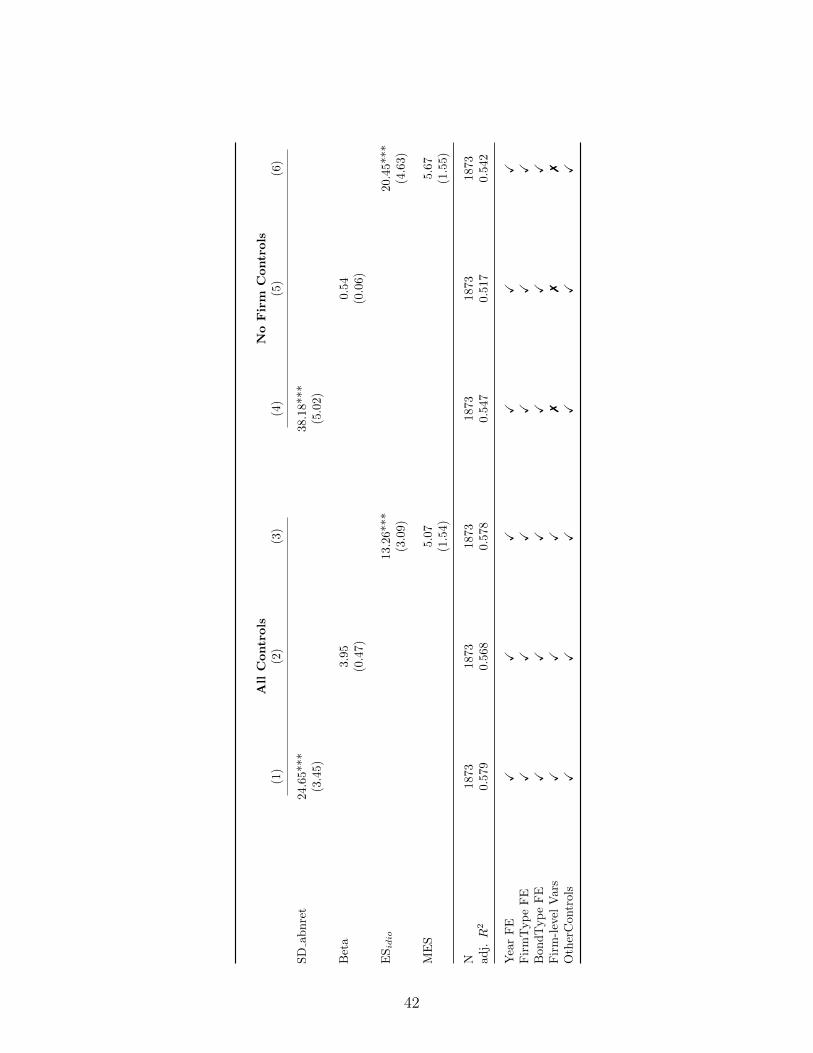
All

Contr

ols

No

Fir

mC

ontr

ols

(1)

(2)

(3)

(4)

(5)

(6)

SD

abnre

t24

.65*

**38

.18*

**(3

.45)

(5.0

2)

Bet

a3.

950.5

4(0

.47)

(0.0

6)

ESidio

13.

26**

*20.4

5***

(3.0

9)

(4.6

3)

ME

S5.

075.6

7(1

.54)

(1.5

5)

N18

7318

7318

7318

731873

1873

adj.

R2

0.57

90.

568

0.57

80.

547

0.5

17

0.5

42

Yea

rF

EX

XX

XX

XF

irm

Typ

eF

EX

XX

XX

XB

ondT

yp

eF

EX

XX

XX

XF

irm

-lev

elV

ars

XX

X7

77

Oth

erC

ontr

ols

XX

XX

XX

42

Table V: Bond Characteristics and Pricing of Tail Risk

The following table displays the primary bond yield regressions with dependent variable asbond yield minus closest benchmark treasury yield expressed in basis points on firm tail-riskmeasures and other bond characteristics during the period from 1990 to 2010. The analysisconsists of the interaction results of tail-risk measures with bond features which are definedin the following manner: Dummy variable d Sub is set to 1 if the bond is subordinated elseit is set to 0. Dummy variables d LowGrade is set to 1 if it’s rating scale ≥ 5 (A or lowerfor S&P, Fitch and Moodys’) implying they are medium-grade bonds else it is set 0 implyingthey are high-grade bonds (AAA or AA - High-grade AAA and AA bonds constitute about33% of the sample; Medium grade A to BBB constitute 63% and the rest 4% are speculativegrade bonds). Similarly d LongMat is set to 1 if the years to maturity of the bond is ≥ 10(the mean and median maturity in the sample is close to 10 years) else it is set to 0. Our tailrisk measures are defined as: ES: the negative of the average of the firm’s daily returns on5% worst return days during the calendar year for the firm; MES: the negative of the averagefirm’s daily return on 5% worst return days of the market (S&P 500 instead of for the firm)during the calendar year; ES, MES are expressed in percentage terms. Rating is generated byconverting the bond ratings to a cardinal scale measured on a 23 point scale for ratings issuedby S&P, Moody’s and Fitch and then taking their average for a given firm. The firms arecategorized into 4 firm-types: Depositories (2-digit SIC code=60); Broker-Dealers (4-digit SICcode=6211); Insurance (2-digit SIC code=60 & 64); Other (2-digit SIC code=61, 62(except6211), 65, 67). Standard bond yield regression controls which are defined in Appendix Band included in the regression specification are: log assets, profitability, long-term debt toassets, leverage, term spread, log issue size, years to maturity. Firm-type fixed effects (FE)are included by defining a dummy variable d Firm-Type for each firm-type that is set to 1 ifa firm belongs to that firm-type or else it is set to 0. Bond-type fixed effects are controlled byincluding dummy variables d Agency, d Sub and d Callable. Year fixed effects are includedin the regressions. All standard errors are clustered at firm level to correct for correlationacross observations of a given firm. All t-statistics are displayed in brackets. *, ** and ***indicate significance greater than 10%, 5% and 1%, respectively.

43

Subordinated Low Grade Bond Maturity(1) (2) (3) (4) (5) (6)

ES 7.50** -0.38 11.36***(2.18) (-0.09) (2.98)

MES 3.15 -4.34 3.92(0.96) (-0.92) (1.06)

d Sub×ES 11.72**(2.10)

d Sub×MES 2.27(0.31)

d LowGrade×ES 18.36***(4.72)

d LowGrade×MES 14.65***(3.09)

d LongMat×ES -3.63(-1.08)

d LongMat×MES -1.13(-0.31)

d Sub 2.42 1.61 13.85* 13.38 4.32 4.66(0.29) (0.18) (1.74) (1.61) (0.48) (0.51)

d LowGrade 5.64 2.61(0.74) (0.34)

d LongMat 8.41* 6.32(1.86) (1.27)

ΣCoeff 19.22*** 5.42 17.98*** 10.31*** 7.73** 2.80(3.37) (0.74) (5.05) (2.81) (2.34) (0.79)

N 1873 1873 1873 1873 1873 1873adj. R2 0.580 0.569 0.563 0.542 0.574 0.565

Year FE X X X X X XFirmType FE X X X X X XBondType FE X X X X X XRating X X 7 7 X XMaturity X X X X 7 7OtherControls X X X X X X

44

Table VI: Firm Characteristics and Pricing of Tail Risk

The following table displays the primary bond yield regressions with dependent variable asbond yield minus closest benchmark treasury yield expressed in basis points on firm tail-riskmeasures and other firm characteristics during the period from 1990 to 2010. The analysisconsists of the interaction results of tail-risk measures with firm features which are definedin the following manner: d Large is a dummy variable set to 1 if the log of firm assets isgreater than the median in the universe of financial firms in COMPUSTAT, else it is setto 0. d HighLeverage is a dummy variable set to 1 if the firm leverage is greater than themedian in the universe of financial firms in COMPUSTAT, else it is set to 0. d Agency is setto 1 if the bond is an agency bond else it is set to 0. Our tail risk measures are defined as:ES: the negative of the average of the firm’s daily returns on 5% worst return days duringthe calendar year for the firm; MES: the negative of the average firm’s daily return on 5%worst return days of the market (S&P 500 instead of for the firm) during the calendar year;ES, MES are expressed in percentage terms. Rating is generated by converting the bondratings to a cardinal scale measured on a 23 point scale for ratings issued by S&P, Moody’sand Fitch and then taking their average for a given firm. The firms are categorized into 4firm-types: Depositories (2-digit SIC code=60); Broker-Dealers (4-digit SIC code=6211);Insurance (2-digit SIC code=60 & 64); Other (2-digit SIC code=61, 62(except 6211), 65, 67).Standard bond yield regression controls which are defined in Appendix B and included in theregression specification are: log assets, profitability, long-term debt to assets, leverage, termspread, log issue size, years to maturity. Firm-type fixed effects (FE) are included by defininga dummy variable d Firm-Type for each firm-type that is set to 1 if a firm belongs to thatfirm-type or else it is set to 0. Bond-type fixed effects are controlled by including dummyvariables d Agency, d Sub and d Callable. Year fixed effects are included in the regressions.All standard errors are clustered at firm level to correct for correlation across observationsof a given firm. All t-statistics are displayed in brackets. *, ** and *** indicate significancegreater than 10%, 5% and 1%, respectively.

45

Assets Leverage Agency Debt(1) (2) (3) (4) (5) (6)

ES 17.97*** 10.82** 11.62***(3.33) (2.44) (3.43)

MES 10.30 2.26 4.99(1.51) (0.50) (1.55)

d Large*ES -10.14*(-1.72)

d Large*MES -5.98(-0.86)

d Leverage*ES -0.77(-0.16)

d Leverage*MES 0.66(0.13)

d Agency*ES -29.98***(-5.35)

d Agency*MES -32.84***(-4.40)

d Large -16.45 -18.26(-1.58) (-1.49)

d Leverage 13.43 19.31*(1.33) (1.90)

d Agency -3.03 -1.15 12.35 14.57 -12.98 -5.67(-0.18) (-0.07) (0.78) (0.90) (-0.74) (-0.31)

ΣCoeff 7.83** 4.32 10.05*** 2.92 -18.36*** -27.85***(2.31) (1.32) (2.74) (0.79) (-3.37) (-3.95)

N 1873 1873 1873 1873 1873 1873adj. R2 0.581 0.570 0.573 0.565 0.581 0.571

Year FE X X X X X XFirmType FE X X X X X XBondType FE X X X X X XLogAssets 7 7 X X X XLeverage X X 7 7 X XRatingScale X X X X X XOtherControls X X X X X X

46

Table VII: Pricing of Tail Risk for Different Institution Types

The following table displays the primary bond yield regressions with dependent variableas bond yield minus closest benchmark treasury yield expressed in basis points on firmtail-risk measures and other firm and bond characteristics during the period from 1990 to2010 separately for each firm type. Our tail risk measures are defined as: ES: the negativeof the average of the firm’s daily returns on 5% worst return days during the calendar yearfor the firm; MES: the negative of the average firm’s daily return on 5% worst return daysof the market (S&P 500 instead of for the firm) during the calendar year; ES, MES areexpressed in percentage terms. Rating is generated by converting the bond ratings to acardinal scale measured on a 23 point scale for ratings issued by S&P, Moody’s and Fitchand then taking their average for a given firm. The firms are categorized into 4 firm-types:Depositories (2-digit SIC code=60); Broker-Dealers (4-digit SIC code=6211); Insurance(2-digit SIC code=60 & 64); Other (2-digit SIC code=61, 62(except 6211), 65, 67). Standardbond yield regression controls which are defined in Appendix B and included in the regressionspecification are: log assets, profitability, long-term debt to assets, leverage, term spread, logissue size, years to maturity. Firm-type fixed effects (FE) are included by defining a dummyvariable d Firm-Type for each firm-type that is set to 1 if a firm belongs to that firm-typeor else it is set to 0. Bond-type fixed effects are controlled by including d Agency, d Suband d Callable which are dummy variables set to 1 if the type of bond is an agency debt,subordinated or callable respectively or else they are set to 0. Year fixed effects are includedin the regressions. All standard errors are clustered at firm level to correct for correlationacross observations of a given firm. All t-statistics are displayed in brackets. *, ** and ***indicate significance greater than 10%, 5% and 1%, respectively.

Panel A analyzes the effect of tail-risk on bond issuance yields controlling for all ourbond-level, firm-level and macroeconomic variables. Panel B analyzes the incremental effectof tail-risk on subordinated bond issuance yields controlling for all our bond-level, firm-leveland macroeconomic variables.

47

Panel A: Only Tail Risk

Depository Broker-Dealer Insurance Other(1) (2) (3) (4) (5) (6) (7) (8)

ES -1.45 37.92*** 11.85* 15.56***(-0.22) (3.34) (1.68) (3.57)

MES -8.57 35.68*** 16.28** 5.23(-0.98) (3.59) (2.44) (1.10)

N 470 470 228 228 269 269 906 906adj. R2 0.476 0.478 0.494 0.483 0.552 0.558 0.656 0.635

Year FE X X X X X X X XBondType FE X X X X X X X XOtherControls X X X X X X X X

Panel B: Tail Risk×Subordinated

Depository Rest(1) (2) (3) (4)

ES -7.23 10.85***(-0.89) (2.88)

d Sub×ES 14.91*** 13.56(2.85) (1.60)

MES -8.80 7.78**(-0.81) (2.12)

d Sub×MES 0.61 14.69(0.06) (1.49)

d Sub 4.08 5.00 11.85 21.73(0.42) (0.43) (0.92) (1.51)

ΣCoeff 7.68 -8.19 24.41*** 22.47**(1.20) (-1.00) (3.10) (2.22)

N 470 470 1403 1403adj. R2 0.484 0.477 0.616 0.604

Year FE X X X XFirmType FE 7 7 X XBondType FE X X X XOtherControls X X X X

48

Table

VII

I:P

oli

tica

lC

onnect

edness

and

Pri

cing

of

Tail

Ris

k

The

follow

ing

table

dis

pla

ys

the

pri

mar

yb

ond

yie

ldre

gres

sion

sw

ith

dep

enden

tva

riab

leas

bon

dyie

ldm

inus

clos

est

ben

chm

ark

trea

sury

yie

ldex

pre

ssed

inbas

isp

oints

onfirm

tail-r

isk

mea

sure

san

dot

her

firm

and

bon

dch

arac

teri

stic

sduri

ng

the

per

iod

from

1998

to20

10.

Our

tail

risk

mea

sure

sar

edefi

ned

as:

ES

:th

eneg

ativ

eof

the

aver

age

ofth

efirm

’sdai

lyre

turn

son

5%w

orst

retu

rnday

sduri

ng

the

cale

ndar

year

for

the

firm

;M

ES

:th

eneg

ativ

eof

the

aver

age

firm

’sdai

lyre

turn

on5%

wor

stre

turn

day

sof

the

mar

ket

(S&

P50

0in

stea

dof

for

the

firm

)duri

ng

the

cale

ndar

year

;E

S,

ME

Sar

eex

pre

ssed

inp

erce

nta

gete

rms.

Rat

ing

isge

ner

ated

by

conve

rtin

gth

eb

ond

rati

ngs

toa

card

inal

scal

em

easu

red

ona

23p

oint

scal

efo

rra

tings

issu

edby

S&

P,

Moody’s

and

Fit

chan

dth

enta

kin

gth

eir

aver

age

for

agi

ven

firm

.T

he

firm

sar

eca

tego

rize

din

to4

firm

-typ

es:

Dep

osit

orie

s(2

-dig

itSIC

code=

60);

Bro

ker-

Dea

lers

(4-d

igit

SIC

code=

6211

);In

sura

nce

(2-d

igit

SIC

code=

60&

64);

Oth

er(2

-dig

itSIC

code=

61,

62(e

xce

pt

6211

),65

,67

).Sta

ndar

db

ond

yie

ldre

gres

sion

contr

ols

whic

har

edefi

ned

inA

pp

endix

Ban

din

cluded

inth

ere

gres

sion

spec

ifica

tion

are:

log

asse

ts,

profi

tabi

lity

,lo

ng-

term

debt

toas

sets

,le

vera

ge,

term

spre

ad,

log

issu

esi

ze,

year

sto

mat

uri

ty.

Fir

m-t

yp

efixed

effec

ts(F

E)

are

incl

uded

by

defi

nin

ga

dum

my

vari

able

dF

irm

-Typ

efo

rea

chfirm

-typ

eth

atis

set

to1

ifa

firm

bel

ongs

toth

atfirm

-typ

eor

else

itis

set

to0.

Bon

d-t

yp

efixed

effec

tsar

eco

ntr

olle

dby

incl

udin

gdAgency

,dSub

anddCallable

whic

har

edum

my

vari

able

sse

tto

1if

the

typ

eof

bon

dis

anag

ency

deb

t,su

bor

din

ated

orca

llab

lere

spec

tive

lyor

else

they

are

set

to0.

All

stan

dar

der

rors

are

clust

ered

atfirm

leve

lto

corr

ect

for

corr

elat

ion

acro

ssob

serv

atio

ns

ofa

give

nfirm

.A

llt-

stat

isti

csar

edis

pla

yed

inbra

cket

s.*,

**an

d**

*in

dic

ate

sign

ifica

nce

grea

ter

than

10%

,5%

and

1%,re

spec

tive

ly.

To

study

the

impac

tof

pol

itic

alco

nnec

tednes

s,w

euse

lobbin

gex

pen

dit

ure

dat

afr

omth

eC

ente

rfo

rR

esp

onsi

veP

olit

ics

(CR

P)

whic

hco

mpiles

dat

afr

omlo

bbyin

gdis

clos

ure

rep

orts

file

dw

ith

Sec

reta

ryof

the

Sen

ate’

sO

ffice

ofP

ublic

Rec

ords

(SO

PR

).T

he

dat

aco

vers

lobbyin

gac

tivit

yth

atto

okpla

cefr

om19

98to

2010

.L

obbyin

gre

cord

sar

em

atch

edw

ith

our

dat

aset

onth

enam

ean

dth

ebro

adin

dust

rycl

assi

fica

tion

ofth

efirm

.P

olit

ical

connec

tednes

sis

defi

ned

intw

ow

ays

-a

dum

my

vari

able

dP

olit

ical

Con

nec

tion

equal

to1

ifth

efinan

cial

firm

has

ever

lobbie

dth

ego

vern

men

tan

d0

other

wis

e;an

dT

otal

Lob

byA

mou

nt(

log)

asth

enat

ura

llo

gari

thm

ofth

eam

ount

ofto

tal

lobbyin

gex

pen

dit

ure

since

the

year

ofdat

aav

aila

bilit

yin

1998

.

49

Fu

llp

eri

od

:1998-2

010

Non

-Cri

sis

Peri

od

:2001Q

2-2

008Q

2(1

)(2

)(3

)(4

)(5

)(6

)(7

)(8

)

ES

19.9

9***

11.6

3***

37.7

4***

15.8

3***

(4.0

4)(3

.05)

(5.0

7)

(2.9

2)

ME

S10.2

7*

4.3

426.6

4**

7.6

3(1

.72)

(1.1

5)

(2.0

6)(1

.08)

dP

olit

ical

Con

nec

tion

*ES

-12.

30**

-32.7

8***

(-2.

41)

(-3.9

1)

dP

olit

ical

Con

nec

tion

*ME

S-8

.28

-28.1

3**

(-1.3

4)

(-1.

99)

Tot

alL

obby

Am

ount(

log)

*ES

-0.8

5**

-2.3

1***

(-2.3

4)

(-3.8

1)

Tot

alL

obby

Am

ount(

log)

*ME

S-0

.52

-1.8

2*

(-1.1

7)(-

1.8

3)

dP

olit

ical

Con

nec

tion

-3.7

9-6

.32

-29.

17*

-31.3

4(-

0.34

)(-

0.5

4)

(-1.6

6)

(-1.4

0)

Tot

alL

obby

Am

ount(

log)

0.2

80.1

4-1

.67

-1.5

9(0

.31)

(0.1

5)

(-1.1

7)

(-0.9

5)

ΣC

oeff

7.69

*1.9

94.9

6-1

.49

(1.8

1)(0

.50)

(0.8

0)

(-0.2

0)

N99

7997

997

997

614

614

614

614

adj.

R2

0.47

90.

462

0.4

78

0.4

62

0.348

0.3

02

0.3

48

0.3

01

Yea

rF

EX

XX

XX

XX

XF

irm

Typ

eF

EX

XX

XX

XX

XB

ond

Typ

eF

EX

XX

XX

XX

XO

ther

Con

trol

sX

XX

XX

XX

X

50

Table IX: Pricing of Tail Risk Around Crisis Periods

The following table displays the primary bond yield regressions with dependent variable asbond yield minus closest benchmark treasury yield expressed in basis points on firm tail-riskmeasures and other firm and bond characteristics during the crisis periods from 1990 to2010. Our tail risk measures are defined as: ES: the negative of the average of the firm’sdaily returns on 5% worst return days during the calendar year for the firm; MES: thenegative of the average firm’s daily return on 5% worst return days of the market (S&P 500instead of for the firm) during the calendar year; ES, MES are expressed in percentage terms.Rating is generated by converting the bond ratings to a cardinal scale measured on a 23point scale for ratings issued by S&P, Moody’s and Fitch and then taking their average for agiven firm. The firms are categorized into 4 firm-types: Depositories (2-digit SIC code=60);Broker-Dealers (4-digit SIC code=6211); Insurance (2-digit SIC code=60 & 64); Other(2-digit SIC code=61, 62(except 6211), 65, 67). Standard bond yield regression controlswhich are defined in Appendix B and included in the regression specification are: log assets,profitability, long-term debt to assets, leverage, term spread, log issue size, years to maturity.Firm-type fixed effects (FE) are included by defining a dummy variable d Firm-Type foreach firm-type that is set to 1 if a firm belongs to that firm-type or else it is set to 0.Bond-type fixed effects are controlled by including d Agency, d Sub and d Callable whichare dummy variables set to 1 if the type of bond is an agency debt, subordinated or callablerespectively or else they are set to 0. All standard errors are clustered at firm level to correctfor correlation across observations of a given firm. All t-statistics are displayed in brackets.*, ** and *** indicate significance greater than 10%, 5% and 1%, respectively.

To study the impact of crisis periods, we construct bond issuance samples of all thefinancial firms in a 2-year window around the crisis-period and divide the period into equalpre- and post- crisis periods of four quarters each. Post-crisis dummies are defined in thefollowing manner: For bonds issued between the period 1997:Q4 and 1999:Q3, d LTCMtakes the value 1 for all bonds issued between the 1998:Q4 and 1999:Q3, and 0 otherwise.For bonds issued between the period 1999:Q2 and 2001:Q1 , d Dotcom takes the value 1 forall bonds issued between 2000:Q2 and 2001:Q1, and 0 otherwise. For bonds issued betweenthe period 2007:Q4 and 2009:Q3, d F inCrisis takes the value 1 for all bonds issued between2008:4Q and 2009:Q3, and 0 otherwise.

51

LTCM Dotcom Financial Crisis(1) (2) (3) (4) (5) (6)

ES 27.57** 2.24 43.41***(2.09) (0.31) (3.53)

MES 9.57 -7.04 18.76(1.10) (-1.10) (1.09)

d LTCM×ES -33.16***(-2.92)

d LTCM×MES -16.55**(-2.03)

d DotCom×ES 9.65(1.24)

d DotCom×MES -17.10(-1.36)

d FinCrisis×ES -61.22**(-2.51)

d FinCrisis×MES -74.70***(-3.41)

d LTCM 70.28*** 86.66***(2.77) (4.08)

d DotCom 47.77*** 40.31***(3.81) (2.80)

d FinCrisis 175.59*** 230.37***(2.80) (5.11)

ΣCoeff -5.59 -6.98 11.89 -24.13* -17.82 -55.95***(-0.88) (-1.25) (1.17) (-1.69) (-0.71) (-2.86)

N 154 154 126 126 100 100adj. R2 0.656 0.602 0.364 0.374 0.605 0.626

Year FE 7 7 7 7 7 7FirmType FE X X X X X XBondType FE X X X X X XOtherControls X X X X X X

52

Table X: Credit Ratings and Tail Risk

The following table displays the ordered probit regressions with dependent variable asrating scale on tail risk and other firm characteristics during the period from 1990 to 2010separately for each firm-type. Credit ratings are converted into a cardinal scale starting with1 as AAA(Aaa), 2 as AA+(Aa1), 3 as AA(Aa2), and so on. Our tail risk measures aredefined as: ES: the negative of the average of the firm’s daily returns on 5% worst returndays during the calendar year for the firm; MES: the negative of the average firm’s dailyreturn on 5% worst return days of the market (S&P 500 instead of for the firm) during thecalendar year; ES, MES are expressed in percentage terms. The firms are categorized into4 firm-types: Depositories (2-digit SIC code=60); Broker-Dealers (4-digit SIC code=6211);Insurance (2-digit SIC code=60 & 64); Other (2-digit SIC code=61, 62(except 6211), 65,67). Standard bond yield regression controls which are defined in Appendix B and includedin the regression specification are: log assets, profitability, long-term debt to assets, leverage,term spread, log issue size, years to maturity. Firm-type fixed effects (FE) are included bydefining a dummy variable d Firm-Type for each firm-type that is set to 1 if a firm belongsto that firm-type or else it is set to 0. Bond-type fixed effects are controlled by includingd Agency, d Sub and d Callable which are dummy variables set to 1 if the type of bond is anagency debt, subordinated or callable respectively or else they are set to 0. Year fixed effectsare included in the regressions. All standard errors are clustered at firm level to correct forcorrelation across observations of a given firm. All t-statistics are displayed in brackets. *, **and *** indicate significance greater than 10%, 5% and 1%, respectively.

Panel A analyzes the effect of tail-risk on bond rating assignment by credit ratingagencies controlling for all our bond-level, firm-level and macroeconomic variables. Panel Banalyzes the incremental effect of tail-risk on subordinated bond rating assignment controllingfor all our bond-level, firm-level and macroeconomic variables.

53

Panel A: Only Tail Risk

Depository Broker-Dealer Insurance Other(1) (2) (3) (4) (5) (6) (7) (8)

ES 0.27*** 0.08 0.43*** 0.15***(3.68) (0.37) (4.19) (2.93)

MES 0.21 -0.30 0.38*** 0.16**(1.46) (-1.17) (3.31) (2.34)

N 470 470 228 228 269 269 906 906Pseudo-R2 0.298 0.290 0.368 0.375 0.189 0.175 0.436 0.433

Year FE X X X X X X X XBondType FE X X X X X X X XOtherControls X X X X X X X X

Panel B: Tail Risk×Subordinated

Depository Rest(1) (2) (3) (4)

ES 0.33*** 0.18***(3.77) (3.92)

d Sub×ES -0.17* -0.14(-1.79) (-1.36)

MES 0.17 0.11*(1.12) (1.67)

d Sub×MES 0.09 0.09(0.78) (0.78)

d Sub 1.10*** 1.05*** 0.30 0.39**(7.89) (8.18) (1.49) (1.98)

ΣCoeff 0.16* 0.26* 0.04 0.20(1.94) (1.82) (0.37) (1.54)

N 470 470 1403 1403Pseudo-R2 0.301 0.290 0.376 0.371

Year FE X X X XFirmType FE 7 7 X XBondType FE X X X XFirmControls X X X X

54