do de novo secondary markets affect primary market ... · do de novo secondary markets affect...
TRANSCRIPT
11
Do de novo Secondary Markets Affect Primary MarketInterest Rates? A Case Study of Peer-to-Peer Lending
Michael Reher1
Georgetown University
Abstract
What happens to a security’s rate of return in the primary market when a sec-ondary market for that security is created? This question is discussed in the context of a de novo secondary market for peer-to-peer loans using loan data from the peer-to-peer platform Lending Club. Drawing on existing literature on risk and liquidity premiums, a basic model of primary market loan rates is developed and tested against the data using an event analysis. In brief, the model is a supply-and-demand analysis using basic intuition about risk and liquidity preferences. The model suggests that interest rates could either in-crease or decrease depending on how much risk existed in the primary market loan pool prior to the introduction of the secondary market. Namely, inves-tors with safe portfolios would choose to substitute towards riskier and higher yielding loans, whereas investors with risky portfolios would do the opposite. The data indicate that risk and interest rates rose among safe loans, fell among risky loans, and fell on the whole after Lending Club created a secondary market. These results suggest that, from a regulatory perspective, the deci-sion to permit a fi nancial intermediary to create a secondary market should be informed by the possibility that this innovation could raise risk levels in the primary market.
1 This paper is submitted in completion of the application for honors in International Economics atGeorgetown University.

THE MICHIGAN JOURNAL OF BUSINESS12
I. IntroductionIn the wake of the 2007 Financial Crisis and subsequent credit crunch,
a variety of nontraditional nancial intermediaries expanded to ll the funding gap left by risk averse banks seeking to tighten their balance sheets. Unlike banks, many of these so-called “new intermediaries”, which include peer-to-peer lending platforms like Lending Club and crowd-sourcing networks like OpenIDEO, facilitate direct transfers of funds from lenders to borrowers.2 Be-fore proceeding, though, it is important to touch on the mechanics of the peer-to-peer loan market, which is the subject of this paper.
Peer-to-peer lending platforms are a relatively new institution for chan-neling funds from lenders to household borrowers. As indicated on Lending Club’s website, these platforms directly link borrowers to lenders in online marketplaces, thus bypassing intermediation by a traditional fi nancial institu-tion. In recent years, the successes of platforms like Lending Club and Prosper have elevated peer-to-peer loans to a prominent place in post-crisis discussions of credit markets.3 These platforms directly link lenders and borrowers by al-lowing the lenders to “shop” from among a variety of online borrower profi les. While borrower profi les generally include statistics such as debt-to-income ratio and FICO range, lenders’ inability to further screen often-anonymous borrowers raises the issue of adverse selection. Moreover, because peer-to-peer loans are usually unsecured, lenders could face high losses in the case of default.4 These risks have allowed lenders to earn returns of up to 10%, a signicant premium relative to many other markets.
Accompanying the rise of new fi nancial intermediaries like peer-to-peer platforms, rumors have circulated that banks may play an obsolete role in post-crisis fi nancial markets.5 Regardless of whether the rumors hold true, the ad-vent of these new intermediaries deserves careful thought and analysis. To a certain extent, one can liken the development of such institutions and the loans they originate to the introduction and trading of mortgage-backed securities (MBS). In both cases, nancial innovation led to the creation of new assets and markets which smoothed access to credit; specically, both innovations have
2 For a brief discussion of the distinctions between peer-to-peer, crowdsourcing, and micronance networks, please visit http://blog.lendingclub.com/2010/10/22/microfi nance-crowdfunding-and-peer-to-peer-lending-explained/.
3 For example, the article “Filling the Bank-Shaped Hole” in the December 15, 2012 edition of TheEconomist mentioned that peer-to-peer platforms might capture an increasing share of the consumer creditmarket by making funds available to subprime borrowers.4 “High” losses are meant relativeto loan size, which often does not exceed $10,000.5 In the article “Filling the Bank-Shaped Hole” in the December 15, 2012 edition of The Economist, aprominent U.K. regulator reportedly suggested that banks could forfeit their sizeable share of the creditmarket in the future.

13Do de novo Secondary Markets Affect Primary Market InterestRates?
made it easier for subprime borrowers to obtain funds.6 Moreover, as MBS markets played a pivotal role in the most recent build-up, crash, and recon-struction, these new markets may prove eminently important in years to come.
In particular, the development of secondary trading for peer-to-peer loans resembles, at least remotely, the secondary markets which facilitated MBS turnover. By understanding how the introduction of a secondary peer-to-peer loan market aected the liquidity and risk structure of the underlying loans, one can better develop the kind of macroprudential regulation needed to contain the risks posed by this new market. In addition to furthering our understanding of peer-to-peer lending, such an analysis would also, more broadly, shed light on the dynamics which govern the formation of a de novo secondary market, which is a relatively uncommon event in the fi nancial world. Given the cur-rent pace of fi nancial innovation, understanding such dynamics is critical for entrepreneurs and policymakers alike.
This paper contributes to the literature by investigating how the creation of a secondary market for peer-to-peer loans affected interest rates, in particu-lar liquidity and risk premiums, in the primary market. In doing so, it builds on the literature of peer-to-peer lending, much of which to date has focused on the qualities which make one a successful borrower or lender (Freedman and Jin (2008, 2011); Berger and Gleisner (2009); Ravina (2008)). Specically, this paper innovates by examining peer-to-peer loans in the context of a secondary market and by using data from Lending Club, a dominant player in the indus-try which has, to the author’s best knowledge, been largely excluded from studies of peer-to-peer lending. Drawing on established methods of measuring liquidity and risk premiums (Sarr and Lybek (2002); McCulloch (1975)), this paper aims to identify the different channels through which the development of secondary trading affects primary market interest rates. In the process, it highlights a more general link between primary and secondary markets, fol-lowing a line of studies which has accomplished this task outside the context of peer-to-peer lending (Vickrey and Wright (2010)).
In October 2008, Lending Club received SEC approval to establish a sec-ondary market for its loans, and Prosper followed suit in July 2009. Both plat-forms partner with the brokerage fi rm FOLIOfn to facilitate secondary trades online. Since Lending Club and Prosper are the dominant players in the U.S. 6 Of course mortgage-backed securities also differ in several key ways from loans originated by, say,
peer-to-peer lending platforms. In particular, the payoff structures of the two assets do not bear perfect resemblance, and MBS markets possess a degree of universality lacking in the secondary trading platforms for peer-to-peer loans. Therefore, one should not overstate the similarities between these two assets. However, the fact that both instruments signicantly ease access to credit while remaining directly susceptible to loan default is worth noting. In the future, the peer-to-peer loan market may converge in similarity to the MBS market. For information on a typical peer-to-peer platform, visit https://www.lendingclub.com.

THE MICHIGAN JOURNAL OF BUSINESS14
peer-to-peer industry, and since their loans are relatively similar in size and nature, the time gap between their establishment of secondary markets would allow for an interesting analysis of how this development might have affected interest rates in the primary market for each platform. Unfortunately, because Prosper shut down its operations while under SEC review from October 2008 to July 2009, the scarcity of Prosper loan data in this period inhibits the kind of diference-in-difference exercise between the fi rms which would be ideal. Instead, analysis is focused primarily on Lending Club. In some sense, this situtation represents a blessing in disguise, since it directs the focus to a fi rm-which has, to this point, been largely left out of academic literature. In doing so, it invites future studies to broaden the discussion of peer-to-peer lending by including data from a variety of platforms in addition to Prosper, which has to date been the data provider of choice (Freedman and Jin (2008, 2011); Rigbi (2008); Ravina (2008)). Moreover, as will be discussed below, Lending Club’s business model allows for a particularly interesting analysis of the interplay between liquidity and risk premiums.
According to the liquidity premium theory of interest rates, the establish-ment of a secondary market should reduce rates across loans of all maturities on the primary market. That is, the secondary market makes peer-to-peer loans more liquid, thereby stimulating demand for these loans and pushing down their return. On the other hand, given the availability of a secondary market, primary lenders may have less incentive to select good borrowers, since lend-ers could potentially liquidate risky loans before default or maturity. In this light, the secondary market might increase the underlying risk in the pool of peer-to-peer loans, implying an increase in the risk premium. Therefore, the interest rate effect of a secondary peer-to-peer market could potentially be positive, zero, or negative. One nuance to Lending Club’s business strategy re-quires amending the basic model mentioned above. Specifi cally, Lending Club itself sets interest rates unlike Prosper, which uses an auction-based system. It can be shown that this subtlety could theoretically introduce more credit risk to the loan pool, pushing up interest rates via the risk premium. In particular, this effect would occur when the loan pool contained relatively little risk prior to the secondary market’s creation. On the other hand, if the loan pool already had suffi cient risk, then risk levels and interest rates could potentially fall. This leads to the following hypotheses:
1. If the average credit risk of the loan pool is suffi ciently low, primary market interest rates and risk levels will rise in response to the creation of a secondary market.

15Do de novo Secondary Markets Affect Primary Market InterestRates?
2. If the average credit risk of the loan pool is suffi ciently high, primary market interest rates and risk levels will fall in response to the creation of a secondary market.
Empirically, I will test these hypotheses by using the techniques of an event analysis to compare interest rates and risk levels before and after the introduction of the de novo secondary market.
The paper will be organized as follows. Section 2 discusses relevant lit-erature on elementary interest rate theory, asset liquidity, secondary markets, and peer-to-peer lending. It also describes the basic theoretical framework which informs the empirical part of the study. Section 3 outlines the empirical strategy for measuring interest rate and risk adjustments in the primary market following the creation of the secondary market. It then presents and interprets the results in light of the literature and model based hypotheses. Section 4 summarizes and concludes, mentioning any relevant policy implications and gesturing towards future research.
II. Literature Review and Model
When Lending Club unveiled its online trading platform in October 2008, it established the fi rst secondary market for U.S. peer-to-peer loans. In this sense, the development of the trading platform represented more than a fi rm-specifi c business strategy; it marked the de novo formation of of a secondary market for an asset which beforehand did not exist outside the primary ex-change. The creation of a secondary market occurs relatively infrequently and often has economic effects which feed back into the primary market. In par-ticular, establishing a secondary market injects an asset with liquidity, defi ned by Allen and Gale (2007) as the degree to which an asset can be transformed into consumption at any given time. All else equal, this positive liquidity shock should increase an asset’s value, since it gives investors the opportunity to transform the asset’s expected cash fl ow into current purchasing power. At the same time, though, the option of selling a poor investment on the secondary market might reduce investors’ incentive to screen for good risks on the pri-mary market. Consequently, a stream of bad risks may be introduced into the primary market, depressing the asset’s value via adverse selection.7 Therefore, establishing an aftermarket could have an uncertain net effect on equilibrium 7 As in Akerlof (1970), adverse selection describes a market mechanism where buyers cannot ascertain
the quality of the product offered by sellers and so demand a lower purchase price to hedge against the risk of buying a low quality product. This effect may depress equilibrium prices or even drive all high-quality producers out of the market.

THE MICHIGAN JOURNAL OF BUSINESS16
prices in the primary market. In the context of peer-to-peer loans, the potential for such uncertainty is real and deserves investigation. This paper contributes to our understanding of the relationship between primary and secondary mar-kets by evaluating how the de novo formation of an aftermarket for peer-to-peer loans affected prices and interest rates in the primary exchange.
Broadly speaking, one can decompose a security’s nominal interest rate into four components: real interest rate, expected infl ation, liquidity premium, and risk premium. Fisher (1930) fi rst proposed the relationship between the real rate of interest and expected infl ation. Many studies have since elaborated on the importance of risk and liquidity in determining the nominal rate, includ-ing Blake (2000). Faure (2012) summarizes these relationship succinctly as:
i = r + πe + l + σ
where
• i denotes the nominal interest rate• r denotes the real interest rate• πe denotes the expected infl ation rate• l denotes the liquidity premium• σ denotes the risk premium
Using this formulation as a starting point, it remains to quantify, at least in relative terms, the four components of the nominal peer-to-peer loan rate.8 In the context of this study, it is most important to fi nd suitable metrics for the risk and, in particular, liquidity premiums.
In the literature, methods of estimating liquidity premiums vary based on how a given study understands liquidity. Specifi cally, Sarr and Lybek (2002) observe that an asset’s liquidity can be understood in four dimensions: tight-ness, depth, breadth, and resiliency.9 “Tightness” describes assets with rela-tively small transaction costs, and it is associated with liquidity in the sense that an asset with low transaction costs can more easily be converted to legal tender. “Depth” and “breadth” are volume-based measures which describe, respectively, the volume of orders of a given size (depth) and the diversity of order sizes (breadth) in an asset market. One can consider deep and broad
8 This expression is necessarily simple and is not intended to be a perfectly robust description of interestrate behavior.
9 Starr and Lybek also mention a fi fth dimension called “immediacy,” which describes how quickly orders can be processed. However, because immediacy basically encapsulates the time component of transaction costs, I consider it a subset of “tightness.”

17Do de novo Secondary Markets Affect Primary Market InterestRates?
markets liquid in that their greater volume and variability of order sizes allows for buyers and sellers to be matched more smoothly. “Resiliency” means that an asset’s price quickly returns to its fundamental value after suffering a sig-nifi cant supply or demand shock. A resilient asset is liquid because its relative price stability makes it easier to trade on the secondary market.
Given a particular understanding of liquidity, Sarr and Lybek summarize the various liquidity measures which may be employed. In terms of tightness, a popular measure is the bid-ask spread, defi ned as the difference between bid and ask prices for a given security. Among other costs, the bid-ask spread en-capsulates the cost of asymmetric information, as a dealer may fi nd it diffi cult to execute a sell order if buyers perceive the traded asset to be of low qual-ity (Gregoriou, Ioannidis, and Skerratt , 2005). To absorb any losses resulting from such information asymmetry, the dealer charges a premium which is built into the bid-ask spread. It follows that a lower observed bid-ask spread would imply lower transaction costs, greater tightness, and thus greater liquidity. In terms of depth and breadth, Sarr and Lybek mention several volume based measures of liquidity. In particular, they mention the importance of turnover rate, defi ned as aggregate value of all transactions over a given period divided by average market value of the asset stock in that period.10 Note that the turn-over rate is closely related to the concept of money velocity in that it describes the volume of transactions which occur over a given time interval. High turn-over rates often correlate with greater liquidity since the increased transaction volume makes it easier to match buyers and sellers of a given position.
To assess an asset’s resiliency, Sarr and Lybek discuss several price-based measures such as the Market Effi ciency Coeffi cient (MEC) developed by Has-brouck and Schwartz (1988). The MEC compares variation in long run returns to variation in the short run.11 For a resilient asset, the ratio of these variances should be close to one, since resilience implies that the market quickly corrects any short run deviations from an asset’s intrinsic value. However, as pointed out by Sarr and Lybek, Bernstein (1987) observed that price-ineffi cient mar-kets often exhibit relatively low short run volatility. This effect artifi cially infl ates the MEC, making it an imperfect measure of asset resiliency. As an alternative to the MEC, Sarr and Lybek mention various regression based ap-proaches including the Market-Adjusted Liquidity Method used by Hui and Heubel (1984). This method partials out systematic risk by regressing an as-set’s return on the market return. The squared residuals are then regressed on daily changes in transaction volume. Intuitively, the residuals from the fi rst 10 Mathematically, the turnover rate is defi ned as T = (Σi PiQi)/(SPavg), where PiQi is the value of trade T,
S is the asset stock, and Pavg is the average asset price over the period.11 Mathematically, MEC = Var(Rlr)/(T •Var(Rsr)), where Rlr and Rsr are the long and short run returns,
respectively, and T is the number of short periods per long period.
THE MICHIGAN JOURNAL OF BUSINESS18
regression describe unsystematic volatility, and the coeffi cient on trade vol-ume in the second regression indicates how responsive an asset’s volatility is to volume fl uctuations. Resilient assets should have low volume coeffi cients, since their prices quickly revert to intrinsic levels following short run demand shocks, as proxied by changes in trade volume.
Since liquidity is a desirable quality in a portfolio, illiquid assets must of-ten sell at a discount. In other words, illiquid assets must generate a higher rate of return, or liquidity premium, to compensate for their lack of tightness, depth, breadth, or resiliency. In straightforward terms, one would want to measure the liquidity premium by taking the difference between an asset’s risk-adjusted rate of return and the return on a liquid, riskless asset such as a Treasury Bill. For assets of varying maturities, one could interpolate the riskless, perfectly liquid rate by constructing a zero coupon yield curve (BIS, 2005). In another approach, McCulloch (1975) develops an estimator for the liquidity premium based on expected future spot rates. Specifi cally, he estimates the difference between the forward interest rate and the expected future spot rate, which he defi nes as the liquidity premium, fi nding that a liquidity premium on U.S. gov-ernment securities exists and varies over time. Much of the recent literature on liquidity premiums has focused on the mortgage-backed securities (MBS) market. Of particular interest is how changes in information transparency can affect tightness, and thus liquidity, in the MBS market. For instance, Glaeser and Kallal (1993) fi nd that increases in loan transparency can actually exacer-bate information asymmetries, inhibiting market tightness and raising liquidity premiums. Pagano and Volpin (2012) elaborate on this idea by observing that greater transparency heightens the advantage of sophisticated investors over their average peers. As a result, average investors may succumb to a “win-ner’s curse” by overpaying for securities in the primary MBS market.12 This effectively raises transaction costs and reduces primary market liquidity.13 On the other hand, Pagano and Volpin also show that low levels of transparency
12 The term “winner’s curse” describes the condition whereby the winner of an auction may have overpaid for the item won; similarly, average investors may overpay for securities if they lack the informational advantage of their more sophisticated peers.
13 It is important to distinguish between a market’s liquidity and an asset’s liquidity. As described in Sarr and Lybek, an asset’s liquidity depends primarily on its tightness, depth, breadth, and resiliency. A market’s liquidiy depends both on the liquidity of the assets traded and on the substitutability of these assets. In the case of Pagano and Volpin, the deterioration of primary market liquidity can refer to a decline in asset liquidity, as the large body of unsophisticated, average investors may end up with poorly performing loans which lack tightness and depth on the secondary market. At the same time, primary market illiquidity can be understood in light of the segmentation, or non-substitutability, of loans purchased by sophisticated versus unsophisticated investors. For the remainder of this paper, though, the focus will be on the more narrow concept of asset liquidity rather than the broader idea of market liquidity.

19Do de novo Secondary Markets Affect Primary Market InterestRates?
can diminish liquidity in the secondary market, since sophisticated investors gradually acquire an information advantage over their average peers. As in the previous case, this advantage forces average investors into “winner’s curse” situation whereby they purchase overpriced assets in the secondary MBS mar-ket.
From a policy perspective, liquidity premiums in secondary MBS mar-kets must be monitored, since these premiums can generate feedback loops which affect home loan rates. For example, in 2008 the Federal Reserve be-gan purchasing large volumes of long term Treasuries and mortgage backed securities, a policy which Gagnon et al. (2011) found to signifi cantly reduce liquidity premiums in the MBS market. Indeed, in light of Vickrey and Wright (2010), such reductions in secondary market liquidity premiums can actually lower mortgage rates. Specifi cally, Vickrey and Wright show that to-be-an-nounced (TBA) markets increase MBS liquidity, as these markets effectively allow MBS owners to hedge their positions by purchasing forward contracts in the TBA market.14 However, whereas Vickrey and Wright demonstrate that liquidity gains in the secondary MBS market affect rates in the underlying home loan market, I will investigate whether a similar mechanism plays out for peer-to-peer loans.
As briefl y mentioned above, the establishment of a secondary market for peer-to-peer loans might affect primary market interest rates through the risk channel in addition to the liquidity channel. In particular, investors may have less incentive to select good borrowers on the primary market, since poorly performing loans could be liquidated prematurely through secondary trading. Consequently, the average credit risk in the pool of primary market loans rises, pushing interest rates up via the risk premium and thus potentially offsetting the liquidity effect. However, as summarized by Faure (2012) and Mishkin (2009), risk premiums depend not only on credit quality, but also on the probabilities of loan prepayment and future interest rate spikes. These last two effects dampen asset values by reducing the worth of future cash fl ows. The literature generally suggests that prepayment and interest rate risks are positively correlated with loan length, since a longer time horizon allows for greater likelihood of random shocks affecting prepayment incentives and in-terest rate behavior (Mishkin, 2009). Therefore, risk premiums on peer-to-peer loans should depend both on (i) borrower credit quality as well as (ii) the length of the loan. If, indeed, risk premiums increased with the introduction of a secondary peer-to-peer market, one would expect to see increases in either the average credit risk or time horizon of the underlying loan pool. As will be discussed in the following section, certain aspects of Lending Club’s business 14 In a TBA market, two parties agree on a price for a bundle of securities to be delivered at a future date.

THE MICHIGAN JOURNAL OF BUSINESS20
model simplify the analysis by allowing us to focus primarily on credit quality as opposed to loan length.
While this paper seeks to advance to our understanding of de novo sec-ondary markets, it also aims to contribute to the relatively recent discussion of peer-to-peer lending. Much of the literature on peer-to-peer lending platforms has focused on legal or personal characteristics which affect a borrower’s prob-ability of receiving funds. For example, Rigbi (2008) fi nds that in states with looser anti-usury laws, high risk borrowers have greater chance of becoming funded. On the personal side, Ravina (2008) documents a preference for physi-cally attractive borrowers, as measured by a higher funding likelihood and lower interest rates. She also fi nds evidence of racial discrimination in that, for a given credit quality, black borrowers pay a premium relative to their white peers. Other studies have focused on the impact that social networks have on peer-to-peer loan rates. These social networks exist within the context of a par-ticular peer-to-peer platform; for instance, residents of a particular town may decide to create a network on Lending Club to organize transactions among each other.15 Berger and Gleisner (2009) fi nd that loans made within such networks tend to have lower rates, since lending to a fellow network mem-ber would presumably mitigate information asymmetries. On the other hand, Freedman and Jin (2008) fi nd that, in certain cases, loans made within these social networks may carry higher interest rates because of platform efforts to incentivize group lending. As a result of this incentive scheme, group leaders have less reason to select quality, low interest rate borrowers.16 In terms of studies which focus on the lender’s perspective, Freedman and Jin (2011) fi nd that lenders learn to discern good risks over time, leading to a gradual exit of subprime borrowers from the peer-to-peer market.
In short, this paper contributes to the literature by investigating how the establishment of a de novo secondary market affects primary market interest rates. By placing this question in the context of peer-to-peer lending, it also furthers our understanding of the peer loan market, as the body of literature on peer lending has not yet delved deeply into the issues surrounding secondary trades.17 Moreover, while much of the empirical work on U.S. peer-to-peer lending has relied on data from Prosper, this study is unique in that it uses data provided by Lending Club.18 Looking forward, as more lending platforms emerge, it will become increasingly important to incorporate their loan data
15 This concept can be likened to that of a “Group” on Facebook.16 In particular, Prosper engaged in such an incentive scheme at the time of Freedman and Jin’s study.17 At least, to the best of the author’s knowledge, the literature has not yet delved deeply into this
question.18 For instance, Freedman and Jin (2008, 2011), Ravina (2007) and Rigbi (2008) all used Prosper data in
their studies.

21Do de novo Secondary Markets Affect Primary Market InterestRates?
into the literature, thereby evaluating whether previously established results on peer-to-peer lending apply to the different fi rms in the industry.
2.2 Model
Using the simple formulation described above, write the nominal interest
rate on a peer-to-peer loan as
i = r + πe + lp(l) + rp(σ)
where i, r, πe, lp(•), l, rp(•), and σ denote, respectively, the nominal loan rate, the real rate of interest, expected infl ation, the liquidity premium, the liquidity level, the risk premium, and the risk level. Note that the goal of this model is develop a basic, but reasonable intuition as to how loan rates might respond to the introduction of a secondary market. As a result, the model is necessarily simple, sacrifi cing robustness for clarity and mathematical simplicity.
Recall from above that the risk premium should be decreasing in the cred-it quality c and increasing in the length t of the loan. At this point, one might ask why liquidity is not built into the risk term σ, since illiquidity constitutes a particular type of risk. To answer this, I refi ne the defi nition of risk premium to include only those risks which would exogenously affect future cash fl ows. In this simple model, these include default, prepayment, and interest rate risks. As these risks are primarily functions of credit quality and loan length, one can write σ = σ(c, t).
The following section discusses loan rates using a partial equilibrium framework. Defi ne demand and supply, in terms of number of peer loans, by
D = qD(i, πe, l, σ)S = qS(i, πe)
Per the discussion in Mishkin (2009), I let the demand and supply curves have conventional slopes. That is, ∂qd/∂i ≥ 0 and ∂qs/∂i ≤ 0. Note that since interest rates vary inversely with prices, this is roughly equivalent to saying that de-mand is decreasing in price while supply is increasing in price. In other words, on the demand side peer loans are ordinary goods and, on the supply side, they exhibit increasing marginal costs. Moreover, as suggested in the literature, it is reasonable to have ∂qd/∂l ≥ 0 and ∂qd/∂σ ≤ 0. That is, lender demand increases in loan liquidity and decreases in loan risk.
Before proceeding, I will mention two aspects of Lending Club’s business

THE MICHIGAN JOURNAL OF BUSINESS22
strategy which make this analysis unique. First, during the period of analysis, all loans had a 36 month time horizon. In the model, this means that t = 36 is fi xed, and so σ = σ(c, t ). Secondly, unlike Prosper, Lending Club has not used an auction mechanism for determining loan rates. Instead, the company itself set interest rates using a formula based on loan size and borrower credit qual-ity. Specifi cally, Lending Club uses FICO credit scores and “a combination of several indicators of credit risk from the borrowers credit report and loan ap-plication” to divide borrowers into 7 grades, each with 5 sub-grades, for a total of 35 classes of risk. Borrowers are then shifted between classes based on the amount of funds requested. The fi nal interest rate is determined by adding a base rate to a premium based on the borrower’s risk class.19 Lastly, borrowers with FICO scores below 660, debt-to-income ratios of 35% or more, or credit histories of less than 36 months are automatically denied access to funds. With respect to the model, this nuance means that, for a given credit level, equilib-rium interest rates depend not only on loan demand and supply, but also, and perhaps most importantly, on the rate established by Lending Club. Since this rate depends on credit quality and increases in the default risk of a particular loan, we may write i = iL(σ).
Suppose that, prior to the introduction of the secondary market, the initial equilibrium is characterized by
D = qD(i0, l0, σ0)S = qS(i0)i = i0 = iL(σ0)
For notational simplicity, I omit πe from the argument of the demand and supply functions and treat it as a constant, since expected infl ation will not play a signifi cant role in this simple exposition. Note that, at least in relative terms, l0 must be small, since the absence of a secondary market means that loans cannot be liquidated before maturity. Now, suppose that the opening of a secondary market imposes a liquidity shock which raises l to some l*, where l* > l0. All else equal, this shock will increase loan demand across all interest rates and risk levels. Figure 1 illustrates this effect in (q, i) space, with the initial shock described by Arrow 1. If one were to extend the analysis to three-dimensional (q, i, l) space and let l0 = 0, this shock is effectively a movement along the demand plane out of the page and into positive l space.
However, as evident in Figure 1, this shock places the market out of equi-librium: at the initial interest rate, demand exceeds supply. To make the model slightly more realistic, let i, l, and σ denote the average interest rate, liquidity 19 This base rate was 5.05% as of January 2013.

23Do de novo Secondary Markets Affect Primary Market InterestRates?
level, and risk level in the pool of loans, and let q denote the quantity of loans corresponding to those values of i, l, and σ. This clarifi cation reconciles the fact that, in reality, the loan pool may contain a wide spectrum of interest rates, face values, liquidity, and risk, and so an analysis by graph must focus on the mean values, or central tendency, of the pool. Returning to Figure 1, if liquid-ity and expected infl ation are held constant, the only variable in this simple model which can adjust to bring the market into equilibrium is σ. Moreover, σ is the only variable which can endogenously shift the Lending Club rate schedule such that there is a mutual intersection of the supply, demand, and rate schedule curves. Whether σ increases or decreases depends on the inves-tor’s risk preferences and the composition of his portfolio.
On the one hand, with the option of selling loans on the secondary mar-ket, lenders can at least partially hedge themselves against losses from non-performing loans. As a result, they can afford to diversify into higher yield-ing risks; essentially, the additional loan liquidity makes investors willing to confront the potential adverse selection in the peer-to-peer market. As lenders substitute towards riskier borrowers, σ increases and the demand curve shifts in. At the same time, because Lending Club’s interest rate is a function of risk, i(σ) moves up. If loan supply is treated as exogenous with respect to risk and liquidity, then the new equilibrium is at (q*, i*, l*, σ*), where q* < q0, i
* > i0, l* >
l0, and σ* > σ0. This scenario is illustrated in Figure 2, where Arrow 1 indicates the initial shock and Arrow 2 indicates the readjustments which bring the mar-ket into equilibrium.
On the other hand, it could be that an investor’s pre-shock portfolio was risky enough such that, even after the liquidity shock, it benefi ts him little to increase the portfolio’s underlying level of risk. In other words, at the new liquidity level and with the same level of risk, the investor’s marginal return to risk, in terms of utility, is relatively small or perhaps even negative. Moreover, because the liquidity shock increased loan desirability, the investor and like-minded peers would be willing to receive a lower interest rate across loans. This willingness can be seen in the lower interest rate associated with the post-shock intersection of demand and supply curves in Figure 1. Put differently, the positive demand shock associated with the de novo secondary market forces investors to accept a lower rate of return. However, because of Lend-ing Club’s rate setting mechanism, the only way that interest rates can come down is through a reduction in risk. Therefore, if investors do not adjust their portfolio risk upwards, competition with other investors forces them to accept a lower rate of return, which occurs through a substitution to less risky loans. In the fi nal equilibrium, q* > q0, i
* < i0, l* > l0, and σ* < σ0. Figure 3 illustrates
this scenario.

THE MICHIGAN JOURNAL OF BUSINESS24
Figure 1: Initial liquidity shock
Figure 2: Liquidity shock with fi xed loan supply curve (case σ* > σ0)

25Do de novo Secondary Markets Affect Primary Market InterestRates?
Figure 3: Liquidity shock with fi xed loan supply curve (case σ* < σ0)
This discussion begs the question of what determines whether risk in-creases or decreases to bring the system into equilibrium. In short, the an-swer depends on how strongly the investor’s interest rate schedule, or demand curve, responds to an increase in risk when compared to the response of Lend-ing Club’s rate setting schedule, which can be thought of as an elastic supply curve. Mathematically, we must compare ∂iD/∂σ and diL/dσ, where iD = iD(qD, l, σ) represents the inverse demand curve and iL= iL(σ) is Lending Club’s rate set-ting function. That is, iD is the interest rate demanded by investors for a given quantity of loans (qD), the liquidity of those loans (l), and the loans’ risk level (σ). In a competitive equilibrium, the rate set by Lending Club, iL, must equal the rate demanded by investors, iD; otherwise, the market will not clear. In par-ticular, if ∂iD/∂σ ≤ diL/dσ, then the market will converge to an equilibrium with average risk level σ* such that σ* < σ0. In other words, average loan risk will decrease. On the other hand, if ∂iD/∂σ > diL/dσ, then the market may converge to an equilibrium where σ* > σ0.
To see this, observe that the market will be in equilibrium if and only if the triangle A in Figure 1 has zero area. Since A has area equal to ½ (qD(iL, •) − qS(iL))(iL − iM), where iM is the rate associated with the intersection of qS and qD, a suffi cient condition for the area to vanish is that qD(iL, •) − qS(iL) converges to 0 as σ converges to σ*.20 Moreover, this condition is also necessary. Otherwise, one could have a situation where iM equals iL but qD(iL, •) ≠ qS(iL) and hence
20 I use the notation qD(i, •) as a reminder that, in this simple framework, qD is also a function of l and σ, whereas qS is only a function of i. Soon, we will consider the case where qS also depends on σ.

THE MICHIGAN JOURNAL OF BUSINESS26
qD(iM, •) ≠ qS(iM), a contradiction since, by defi nition, iM is the rate at which qD(iM, •) = qS(iM). It follows that A has zero area if and only if qD(iL, •) − qS(iL) converges to 0 as σ converges to σ*. In other words, we need qD(iL, •) = qS(iL) for a market equilibrium.
To understand the conditions under which qD(iL, •) − qS(iL) converges to 0 as σ converges to σ*, I defi ne a function ∆ : σ → R where ∆(σ) = qD(iL(σ), l, σ) − qS(iL(σ)).Differentiating with respect to σ gives
Taking the total differential of qD holding q and l constant and then rearranging terms gives
So by substitution one has
As indicated by the sign pattern above, ∂qD/∂iD > 0, dqS/diS < 0, and diL/dσ > 0, meaning that the second term is always positive whereas the fi rst term is posi-tive if diL/dσ > ∂iD/∂σ and negative if diL/dσ < ∂iD/∂σ.21 Therefore, if diL/dσ ≥ ∂iD/∂σ, then d∆/dσ is guaranteed to be positive. On the other hand, if diL/dσ < ∂iD/∂σ, then d∆/dσ could be negative. Keeping in mind an equilibrium requires that ∆ → 0 as σ → σ*, if d∆/dσ > 0, then σ must decrease to bring the market into equilibrium. Likewise, if d∆/dσ < 0, then σ must increase.
Taken together, these remarks imply that diL/dσ ≥ ∂iD/∂σ guarantees that σ* < σ0 whereas diL/dσ < ∂iD/∂σ could, depending on the elasticity of loan sup-ply, lead to an outcome with σ* > σ0. Specifi cally, with inelastic loan supply, dqS/diS will be close to 0 and so diL/dσ < ∂iD/∂σ implies d∆/dσ < 0 and thus σ* > σ0. In fact, given the general tightening of U.S. credit markets which coin-cided with the secondary market’s creation in late 2008, one may reasonably suppose that borrowers had relatively little infl uence over the interest rate they
21 Although I defi ned some of these expressions earlier without the use of strict inequalities, I will proceed with the use of strict inequalities since it simplifi es the language and does not alter the substance of the discussion

27Do de novo Secondary Markets Affect Primary Market InterestRates?
received, thus corresponding to ineslatic supply. Moreover, given that borrow-ers on peer-to-peer lending platforms might have previously been rejected by credit-tightening banks, they would have had less power to bid down rates on peer loans, and so supply inelasticity would appropriately characterize peer-to-peer markets.
Generally speaking, therefore, low values of ∂iD/∂σ correspond to de-creases in average risk and interest rates, while high values ∂iD/∂σ are associ-ated with the opposite.22 This result supports the intuitive description of inves-tor decision-making mentioned earlier. Namely, we can think of iD as a kind of utility received from a particular investment in the sense that a higher rate of return will, all else equal, increase investor welfare. Therefore, if investors are willing to shoulder more risk at the new liquidity level, then we may say the marginal utility from the added risk, proxied by ∂iD/∂σ, is positive and nontrivial. In other words, ∂iD/∂σ will be large enough such that the market sees an increase in average loan risk and interest rates. Conversely, if inves-tors have little utility to gain from increasing portfolio risk, corresponding to a relatively small value of ∂iD/∂σ, then they will substitute towards safer, lower interest rate loans. On the aggregate level, a low ∂iD/∂σ implies that the market converges to an equilibrium with lower risk and interest rates.
The previous analysis treated loan supply as independent with respect to risk and liquidity. On the one hand, this assumption seems reasonable in that a borrower’s decision to request funds would seem unrelated to whether the loan could, say, be easily liquidated on the secondary market. At the same time, though, the loan supply schedules of individuals with high and low default risks might look fundamentally different. That is, while loan supply may be relatively exogenous with respect to liquidity, it could potentially be endog-enous with respect to risk. In fact, the literature suggests that, for a given inter-est rate and level of principal, risky borrowers may indeed supply more loans. Swain (2007) provides evidence of such in the developing world, fi nding that increases in wealth, agricultural income, and, to a lesser degree, education of Indian borrowers leads them to supply fewer loans. To the extent that wealth, income, and education are negatively correlated with probability of default, this fi nding implies that loan supply increases with risk. Similarly, Magri (2002) fi nds evidence from Italy that income volatility increases loan supply.
However, the literature does not uniformly support the notion that bor-rower riskiness increases loan supply. For instance, Jappelli (1990) suggests that risky borrowers may supply fewer loans because they understand that credit markets would likely refuse them funds. Moreover, Magri (2002) fi nds that income growth, which may correlate to lower default probability, leads 22 “Low” and “High” are meant relative to the magnitude of diL/dσ.

THE MICHIGAN JOURNAL OF BUSINESS28
to greater loan supply. Yet one should be cautious when interpreting these and previous results on loan supply in the context of peer-to-peer lending. In particular, the idea that risky borrowers request fewer loans because they anticipate rejection may apply more to traditional credit markets than to peer-to-peer lending platforms. In fact, when Lending Club opened its trading plat-form in October 2008, borrowers turned down by credit-tightening banks may have found a more welcome source of funds in the peer-to-peer market. In this sense, risk should increase the supply of peer-to-peer loans.
As before, market equilibrium requires that the area of the triangle A in Figure 1 converges to 0 as σ converges to σ*. This, in turn, necessitates that the quantity ∆(σ) = qD(iL(σ), l, σ) − qS(iL(σ), σ) approaches 0 as σ nears its equilib-rium value. Using an argument similar to above, it can be shown that
As the sign pattern indicates, if diL/dσ > ∂iD/∂σ and diL/dσ > −∂iS/∂σ, then d∆/dσ is guaranteed to be positive. Likewise, if diL/dσ < ∂iD/∂σ and diL/dσ < −∂iS/∂σ, then d∆/dσ will be negative. However, any other such case makes the sign of d∆/dσ indeterminate. For example, although the previous discussion implied that diL/dσ > ∂iD/∂σ should result in d∆/dσ > 0, it is now possible that d∆/dσ < 0 if diL/dσ < −∂iS/∂σ. In such a case, because d∆/dσ < 0, the equilibrium risk level and interest rate will actually increase, even though the magnitude of ∂iD/∂σ would suggest otherwise. Graphically, this scenario corresponds to the supply curve shifting out so quickly that an equilibrium occurs after only a small increase in σ.
Clearly, allowing qS to depend on σ complicates the analysis by open-ing up the possibility for supply reactions to override the demand reaction. However, the case of inelastic loan supply allows us to largely rule out such a possibility, as then ∂iS/∂σ is suffi ciently close to 0 that the supply term in d∆/dσ becomes relatively unimportant. Moreover, as discussed above, credit tighten-ing during the period of analysis would mean that borrowers, in particular borrowers turned down from banks, may have had less bargaining power over interest rates, corresponding to inelastic supply. If, indeed, loan supply can be described as inelastic, then we may formulate our hypotheses based on the demand-side relationship between diL/dσ and ∂iD/∂σ.
Nonetheless, while the likely case of inelastic loan supply would allow us to focus primarily on demand mechanics, one should keep the role of supply-side risk reactions in mind during the sections which follow. Even if shifts in the supply curve bear little impact on the fi nal equilibrium, such movements
29Do de novo Secondary Markets Affect Primary Market InterestRates?
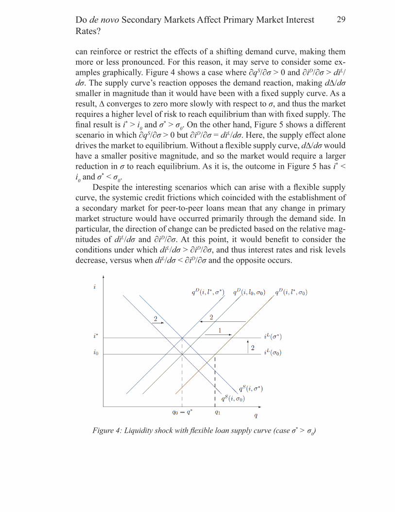
can reinforce or restrict the effects of a shifting demand curve, making them more or less pronounced. For this reason, it may serve to consider some ex-amples graphically. Figure 4 shows a case where ∂qS/∂σ > 0 and ∂iD/∂σ > diL/dσ. The supply curve’s reaction opposes the demand reaction, making d∆/dσ smaller in magnitude than it would have been with a fi xed supply curve. As a result, ∆ converges to zero more slowly with respect to σ, and thus the market requires a higher level of risk to reach equilibrium than with fi xed supply. The fi nal result is i* > i0 and σ* > σ0. On the other hand, Figure 5 shows a different scenario in which ∂qS/∂σ > 0 but ∂iD/∂σ = diL/dσ. Here, the supply effect alone drives the market to equilibrium. Without a fl exible supply curve, d∆/dσ would have a smaller positive magnitude, and so the market would require a larger reduction in σ to reach equilibrium. As it is, the outcome in Figure 5 has i* < i0 and σ* < σ0.
Despite the interesting scenarios which can arise with a fl exible supply curve, the systemic credit frictions which coincided with the establishment of a secondary market for peer-to-peer loans mean that any change in primary market structure would have occurred primarily through the demand side. In particular, the direction of change can be predicted based on the relative mag-nitudes of diL/dσ and ∂iD/∂σ. At this point, it would benefi t to consider the conditions under which diL/dσ > ∂iD/∂σ, and thus interest rates and risk levels decrease, versus when diL/dσ < ∂iD/∂σ and the opposite occurs.
Figure 4: Liquidity shock with fl exible loan supply curve (case σ* > σ0)

THE MICHIGAN JOURNAL OF BUSINESS30
Figure 5: Liquidity shock with fl exible loan supply curve (case σ* < σ0)
In Figure 6, I graphically propose a functional form for iL(σ) and iD(σ, •). Namely, iL(σ) is increasing and linear while iD(σ, •) is increasing and concave. That both functions increase in σ should not cause alarm, as Lending Club’s rate schedule incrementally raises interest rates as credit quality decreases, and investors generally demand a higher rate of return on risky assets. Moreover, the linear nature of iL(σ) seems reasonable, as Lending Club assigns all loans a base rate which it then raises in increments per unit reduction in credit grade. A truly linear function would require that these increments be of equal size. In reality, the increments vary slightly by risk, and so iL(σ) is actually somewhat concave. However, the 0.96 coeffi cient of correlation between increment size and credit grade indicates that iL(σ) has relatively constant slope, and so the idea that it behaves similar to a linear function is not unrealistic. Lastly, the concavity of iD(σ, •) implies not only that investors value safe loans, but that they value them at an increasing rate. Specifi cally, for high values of σ, concav-ity means that ∂iD/∂σ is close to 0. That is, if investors switch from a high risk loan to a slightly safer one, they are only willing to let the risk premium fall by a small amount. On the other hand, for low levels of σ, concavity implies that ∂iD/∂σ will be large. Intuitively, this means that as investors substitute towards a riskless loan, they will accept a large reduction in risk premium. In other words, because lenders prize low risk loans, they are willing to pay increas-ingly more for them. If such risk aversion indeed characterizes the peer-to-peer market, then supposing iD(σ, •) is concave would seem reasonable. Moreover, given the likely presence of adverse selection suggested by the literature, the
31Do de novo Secondary Markets Affect Primary Market InterestRates?
potential for risk among peer-to-peer loans is real and signifi cant.Before proceeding, it should be noted that the functional forms proposed
in Figure 6 are not meant to robustly describe the behavior of iL or iD. Indeed, such a thorough characterization would deserve its own paper. Rather, these conjectures serve as a reasonable premise on which to formulate a hypothesis for the question at hand, which asks whether the de novo secondary market affected primary market interest rates. As such, any conclusions derived from this model serve as, at best, a judicious guess to be tested against the data. Nonetheless, to the extent that this simple model adequately describes the mar-ket, it can provide important insight into the market mechanisms at play, giv-ing the empirical results a practical and economic interpretation.
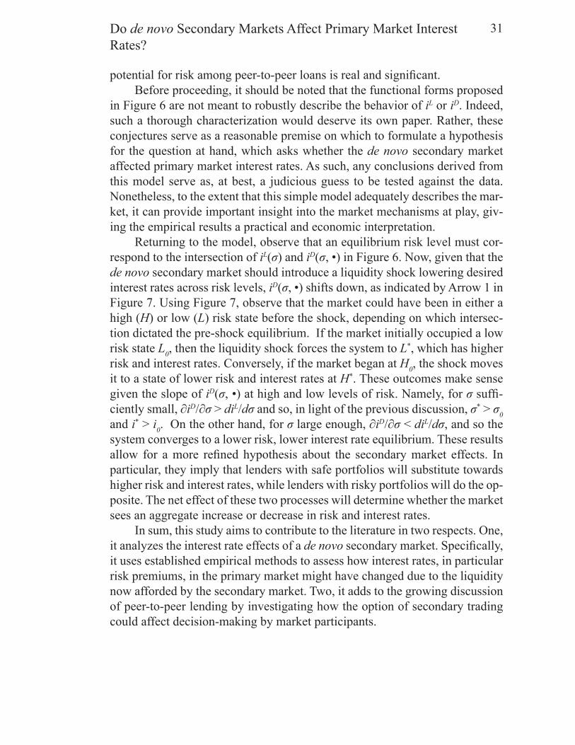
Returning to the model, observe that an equilibrium risk level must cor-respond to the intersection of iL(σ) and iD(σ, •) in Figure 6. Now, given that the de novo secondary market should introduce a liquidity shock lowering desired interest rates across risk levels, iD(σ, •) shifts down, as indicated by Arrow 1 in Figure 7. Using Figure 7, observe that the market could have been in either a high ( H) or low (L) risk state before the shock, depending on which intersec-tion dictated the pre-shock equilibrium. If the market initially occupied a low risk state L0, then the liquidity shock forces the system to L*, which has higher risk and interest rates. Conversely, if the market began at H0, the shock moves it to a state of lower risk and interest rates at H*. These outcomes make sense given the slope of iD(σ, •) at high and low levels of risk. Namely, for σ suffi -ciently small, ∂iD/∂σ > diL/dσ and so, in light of the previous discussion, σ* > σ0 and i* > i0. On the other hand, for σ large enough, ∂iD/∂σ < diL/dσ, and so the system converges to a lower risk, lower interest rate equilibrium. These results allow for a more refi ned hypothesis about the secondary market effects. In particular, they imply that lenders with safe portfolios will substitute towards higher risk and interest rates, while lenders with risky portfolios will do the op-posite. The net effect of these two processes will determine whether the market sees an aggregate increase or decrease in risk and interest rates.
In sum, this study aims to contribute to the literature in two respects. One, it analyzes the interest rate effects of a de novo secondary market. Specifi cally, it uses established empirical methods to assess how interest rates, in particular risk premiums, in the primary market might have changed due to the liquidity now afforded by the secondary market. Two, it adds to the growing discussion of peer-to-peer lending by investigating how the option of secondary trading could affect decision-making by market participants.

THE MICHIGAN JOURNAL OF BUSINESS32
Figure 6: Initial risk response curves for Lend-ing Club (iL) and investors (iD)
Figure 7: Post-shock risk response curves for Lend-ing Club (iL) and investors (iD)

33Do de novo Secondary Markets Affect Primary Market InterestRates?
Figure 8: Post-shock equilibria in (σ, i) space
Data, Empirical Strategy, and ResultsBased on the simple model of interest rates developed above, one might
expect primary market interest rates to rise in response to the establishment of a secondary market for peer-to-peer loans if low risk portfolios dominate the primary market, and one might expect rates to fall if high risk portfolios prevail. Specifi cally, the de novo secondary market should boost loan demand via a positive liquidity shock. In response, lenders could engage the market’s inherent adverse selection and substitute towards riskier loans, bringing the system into an equilibrium with higher average interest rates than the initial state. Alternatively, if lenders gain little utility from riskier investments, they may drive the system to a lower interest rate equilibrium by substituting to-wards safer portfolios. The ultimate effect depends largely on how vigorously investors change their interest rate schedules in response to higher risk. This response function, in turn, depends on the underlying risk of the lender’s cur-rent portfolio, as investors holding safe loans would ostensibly accept an in-crease in risk, and thus an increase in risk premium, with greater enthusiasm than their peers already exposed to risky loans. Therefore, a primary market dominated by low risk portfolios would move towards higher risk and interest

THE MICHIGAN JOURNAL OF BUSINESS34
rates following the introduction of the secondary market. On the other hand, a market comprised of high risk loans would tend in the opposite direction.
Using this framework as a starting point, we should look for two effects: a switch towards new risk levels in the primary market and, correspondingly, a net change in primary market rates. The direction of these changes will depend on aggregate risk in the primary market prior to the creation of the de novo secondary market. In theory, there is also a third effect of interest, which is the initial liquidity shock. However, testing for such a shock would not give par-ticularly interesting results since, given the essential absence of peer-to-peer loan liquidity prior to the secondary market’s creation, the mere ability to trade loans means that the secondary market would have had a positive liquidity ef-fect. As to gauging the size of this positive liquidity shock, the requisite data are not observable, or at least not readily observable, and so the cost of such an endeavor outweighs the benefi t. In particular, the liquidity shock’s magnitude would seem to play little role in determining which equilibrium the market converges to, at least based on the simple model presented earlier. Therefore, this section focuses primarily on testing for the existence and magnitude of the risk and interest rate effects using data from Lending Club’s platform. After fi rst introducing the data, I outline the empirical strategy for testing each effect and then conclude with a discussion of results.
3.1 DataThis study uses loan data from Lending Club’s platform as the observed
primary market data. The sample runs from June 2007 to January 2013 and contains 99,976 observations. Each observation consists of an issued loan along with a set of loan and borrower characteristics. For a full list of loan and borrower characteristics, see Table 1. Among the most important variables are the borrower’s debt-to-income ratio, length of observable credit history, and FICO score range.23 In terms of data density, a new loan was issued on almost every day of the sample. While the frequency of loan origination slowed some-what in the weeks leading up to the creation of a secondary market on October 14, 2008, the data are suffi ciently dense to perform the appropriate analysis on the primary market, as most days saw at least one origination.24 However, one important issue is that, while the primary market data span more than 5 years, we do not observe past data for the secondary market. Specifi cally, Lending Club does not store information on past transactions made through its trading platform.25 Yet, because the emphasis of this study is on primary market effects 23 The FICO score is given over a 5 point interval. Note that FICO scores range from 300 to 850.24 This slowdown in loan origination occurred during a general scaling down of Lending Club’s business
activity while pending SEC approval of the company’s secondary trading platform.25 At least, the data were not made available to the author after several inquiries

35Do de novo Secondary Markets Affect Primary Market InterestRates?
of a de novo secondary market, the empirical strategy relies heavily on primary market data, and so the absence of information on past secondary trades does not pose a signifi cant barrier.p g
3.2 Empirical StrategyEstimating the interest rate and credit risk effects of the de novo secondary
market requires two unique identifi cation strategies. These strategies rely on the notion that a critical event occurred on October 14, 2008 with the unveiling of a secondary market. This structure allows one to exploit variation in the data from before and after the event date, much in the spirit of a conventional event study or regression discontinuity design. With slight modifi cations, I use these conventional procedures to estimate the interest rate and credit risk effects of the de novo secondary market.
To identify the interest rate effect, I perform a modifi ed, or pseudo event study treating newly issued loans as the security of interest and the introduc-tion of a secondary market on October 14, 2008 as the event date. Because variation among borrower credit backgrounds means that each loan carries a different rate of interest, I take the average interest rate among all loans is-sued on a given date as the observed rate of return.26 As in the standard market
26 Strictly speaking, the contract rate on a peer-to-peer loan is not the rate of return, since the rate of return depends also on default probabilities. However, given that higher interest rates correspond to higher return holding risk constant, one can consider the interest rate on peer-to-peer loans as a type of rate of return. In any case, using the language “rate of return” has an advantage in that it corresponds to the terminology of a conventional event study, which this procedure aims to simulate.

THE MICHIGAN JOURNAL OF BUSINESS36
model approach, I estimate the security’s expected rate of return conditional on the market return that day (Armitage, 1995). While some specifi cations also include the risk free rate, I omit it from the model because the macroeconomic instability around the event date might jeopardize any security’s reputation as being truly “risk free”. For the proxied market return, I use the 36 month auto loan rate, since these loans bear many resemblances to peer-to-peer loans including an identical length of 36 months and a common categorization as consumer loans.27 However, because securitized auto loans might have experi-enced signifi cant demand fl uctuations around the event date because of the fi -nancial crisis, the auto loan rate may capture macroeconomic effects unrelated to the peer-to-peer market. For this reason, it may be inappropriate to use auto loan rates as the proxied market return, and so I repeat the process using yields on Moody’s AA, A, and BAA corporate bond indices as the market return. The downside with using these indices, though, is that their breadth may dimin-ish any link to peer-to-peer rates. Moreover, these indices contain bonds of various lengths, most of which exceed 3 years. This maturity mismatch would further weaken the link to peer-to-peer loans.
For several reasons, this strategy cannot be considered a true event study. Most importantly, the relatively low transaction frequency, or in this case orig-ination frequency, of peer-to-peer loans slows the pace at which information fi lters into the observed market rate. For example, in 2008, the average stock on the New York Stock Exchange experienced 1,400 trades per day, while Lending Club averaged only 14 newly issued loans per day over the same pe-27 The rates for 36 month auto loans are national averages and were compiled by Bankrate.com.

37Do de novo Secondary Markets Affect Primary Market InterestRates?
riod.28 One wonders if these statistics mean that peer-to-peer loans require 100 times as long to absorb information as stocks on the NYSE, which are typi-cally the focus of event studies. In any case, an “event study” of peer-to-peer loans would require an information response window signifi cantly longer than one day, which is a window length often used in conventional event studies.29 For this reason, the strategy employed here should be considered a pseudo event study. Specifi cally, I lengthen the response window to 150 days. While a clear downside to lengthening the response window is that other, unrelated information could also affect interest rates during the window, a benefi t is that the longer window allows enough transactions to occur so that we can observe the full interest rate impact of the event. Given the very low transaction fre-quency of newly issued peer-to-peer loans relative to stocks traded on the New York Stock Exchange, this benefi t may be well worth the cost.
In the standard market model, the expected rate of return on peer-to-peer loans acts as a linear function of the market interest rate. However, given the lengthy response window, I also include a time trend to avoid confounding genuine changes in market structure with an unrelated, time dependent process such as, say, a gradual increase in interest rates because of credit frictions dur-ing the fi nancial crisis. For this reason I include a time term t in the equation for a loan’s expected rate of return. Thus, the expected interest rate on peer-to-peer loans issued at time t conditional on the market return can be written
E(P2Pt|Markett, t) = α + βMarkett + γt
where the parameters α, β, and γ are constants and will be estimated using Ordinary Least Squares. Also, it should be noted that P2Pt is defi ned as the average interest rate for loans issued on day t. It is common to use the three months prior to the event as the window for estimating model parameters. However, because of reduced data density in the month prior to the event date, corresponding to the slowdown in loan origination which preceded the intro-duction of the secondary market, I use a fi ve month estimation window. While lengthening the estimation window has a drawback in that the estimated model might be outdated by the time of the event, it also has the benefi t of increasing the sample size so that the fi t becomes less susceptible to outliers. Lastly, re-call from above there are four candidates for the proxied market return: the 36 month auto loan rate and Moody’s AA, A, and BAA bond indices. I estimate E(P2Pt|Markett, t) four separate times using each of these rates and then a fi fth time using only the time trend.
28 This statistic came from the NYSE website.29 See, for instance, Gagnon et al. (2011).

THE MICHIGAN JOURNAL OF BUSINESS38
With a traditional event study, one would defi ne the excess interest rate on peer-to-peer loans by et = [E(P2Pt|Markett, t) − P2Pt]. Intuitively, et would represent the deviation in interest rates from what we would otherwise expect on day t given the market’s behavior. Ideally, one would compute et on the event day and interpret this statistic as the interest rate effect of establishing a secondary market. While this strategy would work for an effi cient market, the relatively low frequency of loan origination following the event date means that the primary market may have taken more than one day to respond to the shock of the de novo secondary market. Since I use a 150 day response win-dow, the natural approach would be to compute the average of et over this pe-riod and determine whether it differs signifi cantly from 0. Alternatively, given the lengthy response window, one could also estimate E(P2Pt|Markett, t) over the 150 days before and after the event date and include a binary variable which equals 1 for loans issued after the introduction of the secondary market and 0 otherwise. That is, one would estimate
E(P2Pt|Markett, t) = α + βMarkett + γt + λPostEventt
and interpret λ as the interest rate effect of the de novo secondary market. Furthermore, since the model implies that the interest rate effect might differ based on portfolio risk, I repeat this procedure twice using only high and low risk loans, where low risk is arbitrarily defi ned as an A or B grade on Lending Club’s credit scale.30
As briefl y mentioned above, a signifi cant issue with using such a long re-sponse window is that news unrelated to the de novo secondary market might also be moving primary market interest rates, and so pinpointing the desired interest rate effect becomes increasingly diffi cult. Including a time trend in the market model partially corrects for this by removing any variation due to broad, time-dependent macroeconomic patterns. Moreover, given the peer-to-peer market’s low transaction frequency, any other important event which occurred during the 150 day response window would itself require a lengthy period of time to make its own impact on primary market rates. Thus, there is a natural limit on the ability of such exogenous events to distort interest rates during the response window. Nonetheless, given the general fi nancial upheaval which coincided with the de novo secondary market, one should at least be aware of outside factors which may have shifted peer-to-peer loan rates at this time.30 Recall that the credit scale runs from A to G with fi ve sub-grades per letter, giving a total of 35 classes
of risk. So an A or B grade on the Lending Club scale would correspond to a credit class of 1 through 10. Also, the defi nition of low risk as an A or B grade is meant only as an arbitrary starting point from which appropriate adjustments may be made.

39Do de novo Secondary Markets Affect Primary Market InterestRates?
Namely, towards the end of November 2008, the Federal Reserve an-nounced that it would begin large scale purchases of distressed assets, in par-ticular mortgage-backed securities (MBS). To the extent that peer-to-peer loans can substitute for mortgage-backed securities, this announcement could have reduced demand in the peer-to-peer market as investors shifted towards the MBS now being purchased by the Fed. However, supposing that the second-ary market introduced a positive liquidity shock which boosted loan demand, a shift towards MBS would then oppose this initial effect. As a result, any observed shifts in primary market interest rates would be smaller than with-out the Fed’s announcement. In other words, the Fed’s announcement would reduce the magnitude of the point estimates, giving them the interpretation as a lower bound of the secondary market effect. Even so, to eliminate the effect of the Fed’s announcement, I repeat the above procedure using a one month response window. Then, I perform a fi nal test using a seven day window, com-puting average abnormal return over the seven day period, , and performing a normal, two-sided hypothesis test to determine whether it differs from 0. This second method replicates a traditional event study.31 Of course, a shorter response window risks truncating the full impact of the secondary market, and so these two tests are in a way suboptimal. Nonetheless, they serve as additional robustness checks to the original specifi cation.
Lastly, one should take into consideration the fact that the opening of a secondary market on October 14 may not have surprised investors. In fact, Lending Club had already been under SEC review for several weeks regard-ing the company’s request to establish such a secondary market. Therefore, investors may have already adapted their strategies prior to October 14, and so any interest rate effect of the de novo secondary market may have already been built into the average rate on the primary market. Luckily, this nuance would, if anything, bias the estimates downwards. Thus, the results may be interpreted as a lower bound of the actual interest rate effect of establishing a secondary market.
In the second half of the investigation, which identifi es the credit risk ef-fect, I use a regression discontinuity design to compare the average risk in the pool of newly issued loans before and after the event date, much in the spirit of the pseudo event study above. Within this framework, the subset of loans issued before the event date comprise the control group while those loans is-sued after the event date comprise the treatment group. Defi ne a function c(t)
31 The test statistic equals mean(et)/(sd(et)//// ), where mean(et) and sd(et) are the sample mean and standard deviation of et computed over the seven day event window. Visit dss.princeton.edu for more information on this method.

THE MICHIGAN JOURNAL OF BUSINESS40
which describes the average credit risk of loans issued on day t. The idea is that, if indeed something occurred on the event date t = t* which substantially affected average credit risk, then c(t) should exhibit a point of discontinuity at t*. Practically, one can detect such a point of discontinuity by estimating c(t) using the treatment and control groups separately and then comparing whether a signifi cant difference in the estimate for c(t*) exists between the two models. Such a difference would indicate that c(t) jumped discontinuously at t* with admission to the treatment group. In other words, this would mean that the es-tablishment of a secondary market at t* was associated with a different average level of credit risk among newly issued loans.
This method proceeds in several steps. First, one must defi ne the average credit risk c in the pool of newly issued loans. Then, one must estimate c(t) us-ing the control and treatment groups. Finally, one must compute and interpret the difference in the two estimates for c(t*). As a note of caution, the value of c we are looking for is really the level of perceived risk in the loan pool, rather than the actual risk. In other words, because investors may not gauge risk perfectly, one must distinguish between an actual shift in loan riskiness and a shift in loan characteristics towards what appears risky in investors’ eyes, but which may not necessarily be so. Therefore, c is defi ned in multiple iterations to take into account possible variation in the quality of investor judgment. The fi rst, most robust defi nition of c is the probability of loan default or charge-off conditional on both the borrower’s credit and personal background. Specifi -cally, for each loan issued to borrower i,
ci = Φ(f(Crediti, Personali))
where Φ is the cumulative standard normal distribution function and f is lin-ear. This equation represents the conventional probit model and will be esti-mated accordingly. In the second, more basic defi nition of c, I condition only on credit background and omit personal characteristics from the model. In the above specifi cation, the components of the credit term include the borrower’s debt-to-income ratio, FICO range, and the length of available credit history. Note that these variables mirror those which Lending Club includes in its basic credit rating method.32 The personal term consists of education, employment length, and monthly income. For a complete list of these variables, see Table 1. Lastly, in the third defi nition of c, investors do not determine credit risk them-selves, but instead rely on the credit grade generated by Lending Club. Thus,
32 While Lending Club may take other factors into account when determining credit grades, it explicitly names these three characteristics.

41Do de novo Secondary Markets Affect Primary Market InterestRates?
c simply equals the Lending Club credit grade assigned to a particular loan.33
For each day in the sample, c is averaged across all loans issued that day. This generates a time series ct of average credit risk in the pool of newly issued loans. To determine c(t), I fi t a linear time trend using Ordinary Least Squares. Specifi cally,
c(t) = E(ct) = γ + δt
where γ and δ are parameters to be estimated. For similar reasons as with the pseudo event study, I use the fi ve months before and after the event date as the estimation window for c(t). Also, as before, I include a binary variable indi-cating whether the observation belongs to the post-event, or treatment group. That is, I estimate
c(t) = E(ct) = γ + δt + ωPostEventt
and interpret ω as the estimated risk effect of the secondary market. Moreover, since the model implies that this effect varies based on the riskiness of an in-vestor’s pre-event portfolio, I repeat the procedure for high and low risk loans separately, where, as above, low risk is defi ned as an A or B on Lending Club’s credit scale. Lastly, as with the pseudo event study, investor foreknowledge of the de novo market might mute the estimated risk effect, since lenders may have already adjusted their portfolio by the time the market was formally in-troduced. However, as above, this nuance means that we can interpret ω as a lower bound of the risk effect.
While event based methods allow one to measure the interest rate and credit risk effects of the de novo secondary market, little empirical attention has been paid to using these methods for an investigation of the secondary market’s initial liquidity shock. In fact, given that liquidity encapsulates the cost of converting an asset to purchasing power, it makes little sense to discuss loan liquidity prior to the establishment the secondary market, as at that time the option of converting loans to cash did not exist. In some sense, then, one can characterize pre-secondary market loans as infi nitely illiquid. One might argue that the mere option of selling one’s loans means that the secondary market had an unambiguously non-negative effect on loan liquidity. Therefore, measurements of the liquidity effect are in some way less interesting and less important than estimates of the interest rate and risk effects. Moreover, the fact 33 Recall, again, that Lending Club credit grades range from A to G, each with 5 subclasses. This makes
for a total of 35 categories of risk. In the discussion which follows, the terms “grade” and “score” refer to a loan’s credit quality on this 35-point scale, with a value of 1 corresponding to highest quality and lowest risk.

THE MICHIGAN JOURNAL OF BUSINESS42
that one cannot observe past trades made on the secondary market means that one would have to aggressively extrapolate to determine liquidity around the event period.
Nonetheless, before proceeding, and in light of the literature on measur-ing liquidity premiums in other asset markets, it helps to understand whether liquidity in this study is being understood in terms of tightness, depth, breadth, or resiliency. Since each loan comes from a different borrower, one can think of each loan as a unique security. Therefore, it is diffi cult to describe peer-to-peer loans in terms of resiliency, as there does not exist a collective, universal sell price for all peer-to-peer loans. For a similar reason, volume based ap-proaches may be less applicable to the peer-to-peer loan market, since it is diffi cult to compare the breadth and depth of buy and sell orders for loans of different risk structures.34 On the other hand, because asymmetric information affects all loans on the trading platform, it makes sense to discuss peer-to-peer loans in terms of tightness. Thus, the de novo secondary market most likely improved loan liquidity by opening up the possibility for tight transactions in the aftermarket. This improved liquidity would have then shifted interest rates and risk levels in the primary market. These interest rate and risk effects are the focus of the empirical investigation at hand.
3.3 ResultsOn the whole, interest rates and risk levels for newly issued loans de-
creased following the introduction of the secondary market. Despite this net downward effect, safe loans actually saw an increase of 1.2% to 1.6% in in-terest rates as well as a rise in credit risk. Risky loans, on the other hand, experienced decreases in credit risk and a drop of 0.6% in interest rates. As a result of these opposing effects, interest rates decreased by 1.3% while risk of charge-off decreased by 2.9%. Taken together, these empirical results support the hypothesis that safe portfolios would shift towards riskier, higher yielding loans while riskier portfolios would behave in the opposite fashion. The net effect of these two opposing forces would then determine the fi nal equilibrium.
With respect to interest rates, most specifi cations point to increases for safe loans and decreases for risky loans, leading to a net reduction in interest rates. However, the magnitude and signifi cance of the results vary somewhat by specifi cation. Specifi cally, Table 3 shows that, in the baseline pseudo event study with a 150 day response window, interest rates fell by between 1.2% and
34 If peer-to-peer loans are grouped by risk class, then we might conceive of a more homogenous secondary market for loans of a given risk level. In this context, resiliency, breadth, and depth are more meaningful for peer-to-peer loans.

43Do de novo Secondary Markets Affect Primary Market InterestRates?
1.3% regardless of the market rate used. However, Tables 4 and 5 show that the estimate varies by market rate in the low and high risk specifi cations. At the same time, if one market rate demonstrates a superior ability to describe the behavior of loan rates, then the point estimate produced using that market rate would seem to be most valid. Accordingly, if one determines the optimal rate on the basis of highest adjusted R2, then the net interest rate effect was -1.3% for the entire sample, +1.5% for safe loans, and -0.6% for risky loans.35 Before proceeding, recall that safe loans were arbitrarily defi ned as having a Lending Club score of 10 or less, corresponding to A or B grade loans. However, this defi nition provided inconclusive results, and so, since it was arbitrary, it was modifi ed so that safe loans are now defi ned by a score of 9 or less. This new defi nition produced the results discussed here.p
Interestingly, while the signs of the point estimates conform to the hy-pothesis, their magnitudes might raise some questions. In particular, one might expect the point estimate for the full sample to lie between the estimate for the high and low-risk specifi cations. However, the full sample estimate is even more negative than that of the high-risk specifi cation. On the one hand, given how an observation is defi ned in this analysis, such a discrepancy might not be interesting. Namely, each observation represents a daily average of loan rates; 35 In many cases, the optimal rate was the 36 month auto loan rate, which makes sense given that the
auto loans were of the same maturity as peer-to-peer loans. As an additional check, the pseudo event study was reproduced using the spread between the auto loan rate and the peer-to-peer rate as the dependent variable. This alternative method produced similar results to the baseline test, giving signifi cant estimates of between -1.2% and -1.3% for the net interest rate effect.
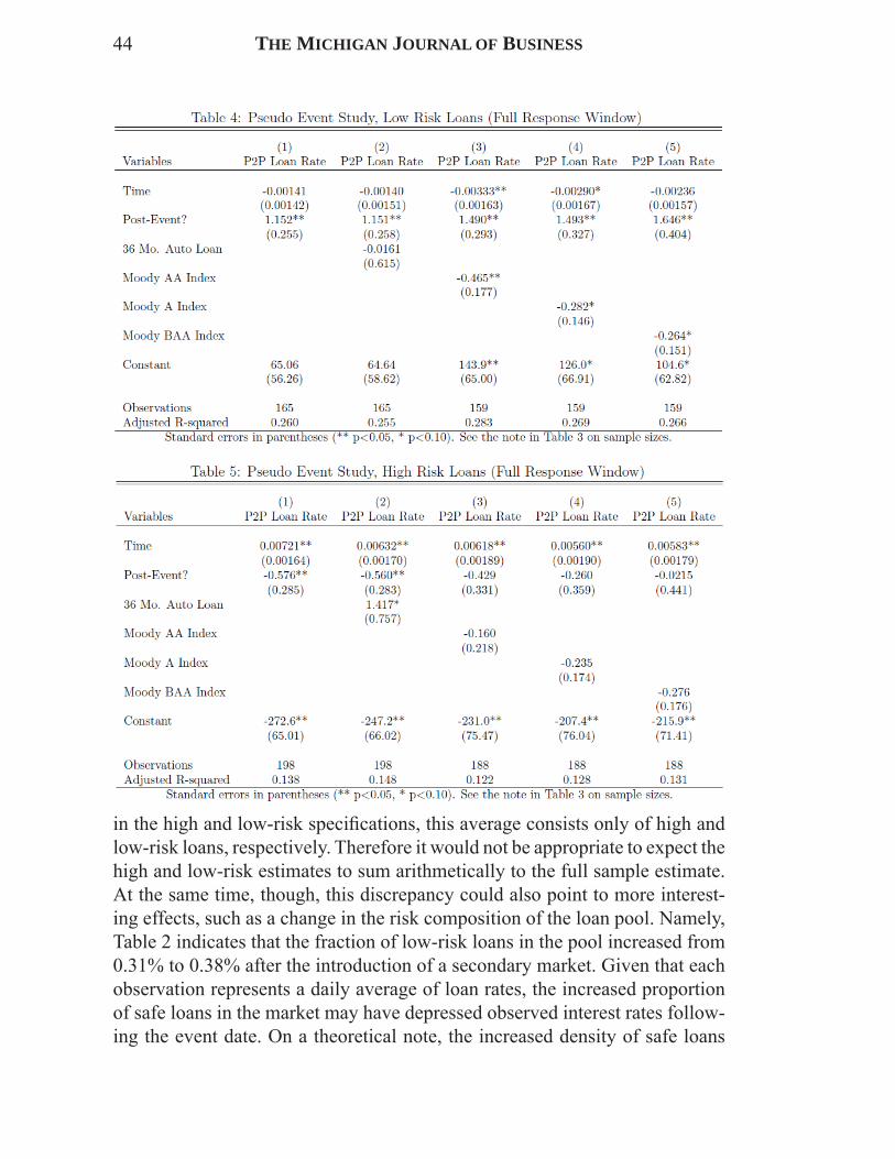
THE MICHIGAN JOURNAL OF BUSINESS44
in the high and low-risk specifi cations, this average consists only of high and low-risk loans, respectively. Therefore it would not be appropriate to expect the high and low-risk estimates to sum arithmetically to the full sample estimate. At the same time, though, this discrepancy could also point to more interest-ing effects, such as a change in the risk composition of the loan pool. Namely, Table 2 indicates that the fraction of low-risk loans in the pool increased from 0.31% to 0.38% after the introduction of a secondary market. Given that each observation represents a daily average of loan rates, the increased proportion of safe loans in the market may have depressed observed interest rates follow-ing the event date. On a theoretical note, the increased density of safe loans

45Do de novo Secondary Markets Affect Primary Market InterestRates?
makes sense in light of the model discussed above. Namely, as illustrated in Figure 3, if high-risk portfolios shift towards safer loans, then we should see an outward shift of the demand curve, corresponding to a higher quantity of loans demanded. That is, as investors substitute towards safety, they demand more loans, leading to a rise in the proportion of low-risk loans in the pool. This effect could, in part, explain why the full sample estimate for the change in loan rates is so negative.
As mentioned earlier, even though a long, 150 day response window probably captures the fullness of the interest rate effect, it may also admit other exogenous information, such as, for example, the Fed’s late November decision to purchase large quantities of mortgage-backed securities.36 For this reason, I repeat the event study using a truncated, one month response window. By and large, this second specifi cation supports the results from the baseline study, as seen in Tables 6 through 8. In particular, if the optimal market rate is again chosen as that providing the highest adjusted R2, then the results indicate net interest rate effects of +0.8% for safe loans, -0.6% for risky loans, and -1.5% for the entire sample. Except for the fact that the risky loan estimate is signifi cant at only 10%, these results reinforce the baseline outcomes. The fact that the estimates are of higher magnitude could mean that the market was still adjusting after one month. Alternatively, it could mean that other news had interfered with loan rates during the interim period, dampening the magnitude of the secondary market’s observed interest rate effect by the end of the fi ve month window. In any case, with reasonable confi dence it appears that loan rates rose for low risk loans, fell for high risk loans, and decreased on the whole by 1.3% to 1.5%.
While the results obtained via the pseudo event studies paint a relatively clear and consistent picture of the interest rate effect, the results obtained with a true event study and a 7 day response window prove less conclusive. In par-ticular, even though the test statistic for safe loans is positive and signifi cant across most market rates, it is insignifi cant for the full sample and the subset of risky loans, as shown in Table 9. Moreover, for risky loans, the test statistic
36 It should also be noted that on October 14, Lending Club increased the base rate for A4 and A5 loans by 0.75% and for B1 through G5 loans by 0.5%. The most conservative way to deal with this change in Lending Club’s rate schedule would be to simply subtract 0.5% to 0.75% from the point estimates, giving a +0.75% to +1.0% interest rate effect for safe loans and signifi cantly negative interest rate effects for both risky loans and the full sample. The key is that the signs of the point estimates do not change. Moreover, recall from the hypothesis that diL/dσ, the slope of the Lending Club rate schedule, should determine the equilibrium. To the extent that this rise in the base rate affected all loan rates within a neighborhood of +0.5% to +0.75%, one might consider this effect a change in the intercept, not the slope, of the Lending Club rate schedule. In this light, one would not expect the change in base rate to have a signifi cant effect on equilibrium outcomes.

THE MICHIGAN JOURNAL OF BUSINESS46
sometimes has a contradictory, positive sign. On the one hand, the fact that the safe loan test statistic is signifi cant and positive reinforces the previous results. On the other hand, the statistical insignifi cance and potential sign contradic-tions for the other two categories might raise some questions. However, keep-ing in mind the peer-to-peer market’s particularly low transaction frequency, or loan issuing frequency, loan rates might have required much more than 7 days to adjust to the new information. Consider, for instance, the peer-to-peer mar-ket’s average frequency of 14 loans per day in 2008 versus the NYSE average of 1,400 transactions per stock per day. In this light, a true event study using only a 7 day response window would seem rather inappropriate for measuring
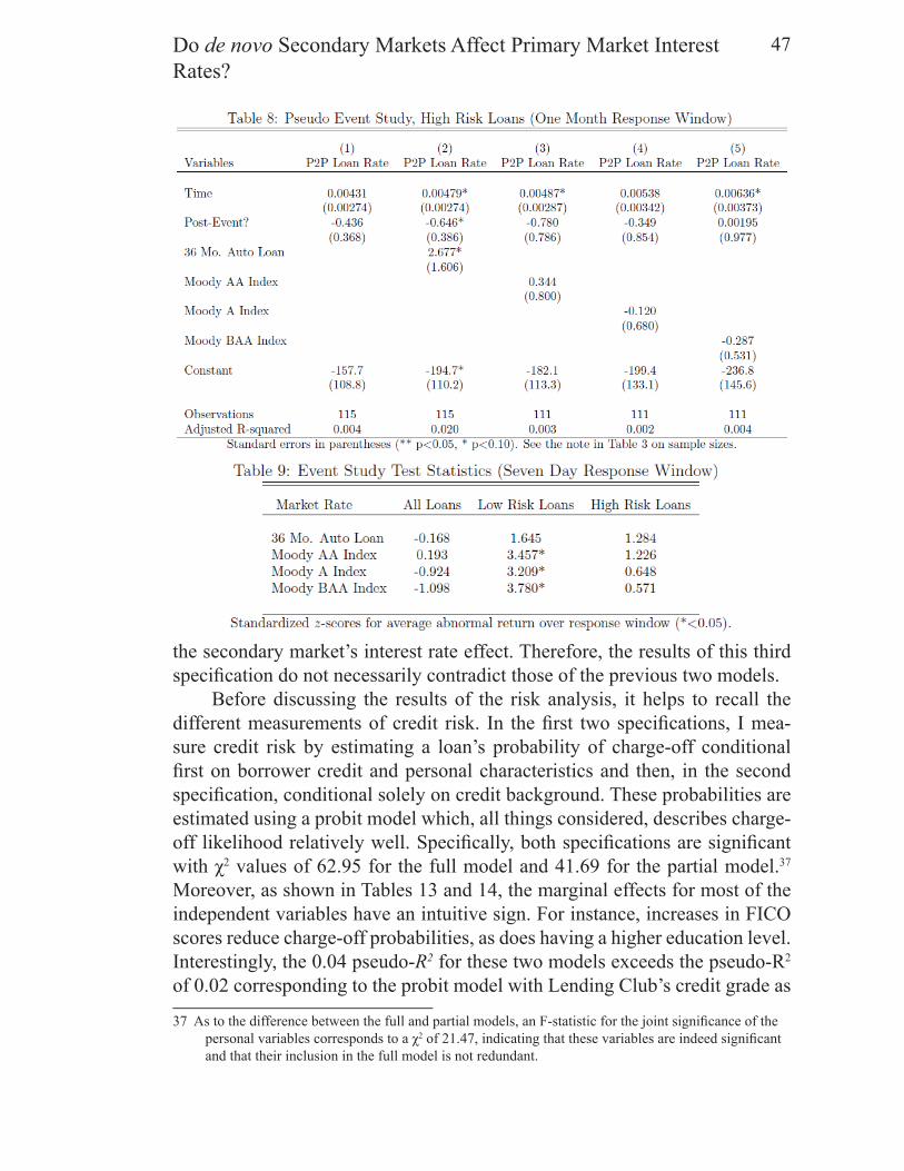
47Do de novo Secondary Markets Affect Primary Market InterestRates?
the secondary market’s interest rate effect. Therefore, the results of this third specifi cation do not necessarily contradict those of the previous two models.
Before discussing the results of the risk analysis, it helps to recall the different measurements of credit risk. In the fi rst two specifi cations, I mea-sure credit risk by estimating a loan’s probability of charge-off conditional fi rst on borrower credit and personal characteristics and then, in the second specifi cation, conditional solely on credit background. These probabilities are estimated using a probit model which, all things considered, describes charge-off likelihood relatively well. Specifi cally, both specifi cations are signifi cant with χ2 values of 62.95 for the full model and 41.69 for the partial model.37 Moreover, as shown in Tables 13 and 14, the marginal effects for most of the independent variables have an intuitive sign. For instance, increases in FICO scores reduce charge-off probabilities, as does having a higher education level. Interestingly, the 0.04 pseudo-R2 for these two models exceeds the pseudo-R2 of 0.02 corresponding to the probit model with Lending Club’s credit grade as
37 As to the difference between the full and partial models, an F-statistic for the joint signifi cance of the personal variables corresponds to a χ2 of 21.47, indicating that these variables are indeed signifi cant and that their inclusion in the full model is not redundant.

THE MICHIGAN JOURNAL OF BUSINESS48
the predictor and charge-off probability as the response. This could indicate that Lending Club’s grading scheme is suboptimal with respect to predicting charge-off likelihood, and so a sophisticated investor might not make deci-sions solely on the basis of the Lending Club grade. This then leads to the third measurement of credit risk, which is simply the Lending Club credit grade. As might be expected, there are close links between these three measurements. In fact, one can obtain a simple conversion formula by regressing charge-off probability, as predicted by the full probit model, on the Lending Club grade. This procedure gives the conversion formula Prob = 0.081 + 0.006 × LCgrade. Using this formula, we can compare results among specifi cations using the probit measurements and that using the Lending Club grade.
As indicated in Tables 10 through 12, credit risk rose for safe loans and

49Do de novo Secondary Markets Affect Primary Market InterestRates?
fell for risky loans, leading to a net reduction in risk. In particular, charge-off probabilities fell by around 3% for the full sample. This result is consistent across measurements of credit risk, as the estimated reduction in Lending Club grade converts to a 2.9% fall in charge-off likelihood, which mirrors the results obtained using the full and partial probit measurements.38 When considering safe and risky loans separately, though, the results prove somewhat less con-sistent. Specifi cally, when using Lending Club’s credit grade as the metric, the risk effects were +1.47 units for safe loans and -2.64 units for risky loans, corresponding to a +0.9% and -1.6% change in charge-off probabilities, re-spectively. On the other hand, the test produced insignifi cant results for both safe and risky loans when using the full probit model to measure risk. This disparity might refl ect lender reliance on the Lending Club grade to gauge risk and make investment decisions, even though this metric is suboptimal relative to the full and partial probit models estimated here. In other words, investors might choose to trust Lending Club’s risk measurements rather than formulat-ing their own models. In this light, credit risk increased among safe loans by around 0.9% and decreased among risky loans by about 1.6%, leading to an aggregate decrease in charge-off probability by 2.9%.
In sum, this investigation points to a reduction in primary market interest rates and risk levels, which can be decomposed into a shift towards risk and return among safe loans and an opposite shift among risky loans. Of note, the results support the core hypothesis regarding post-secondary market inter-est rate and risk behavior. Namely, with the additional loan liquidity afforded by the secondary market, lenders dealing in safe investments became willing 38 This is computed as d(Prob)/d(LCgrade) × ∂(LCgrade)/∂(PostEvent) = 0.006 × −4.864 = −0.029.

THE MICHIGAN JOURNAL OF BUSINESS50
to diversify towards riskier, higher-yielding loans. After all, such loans had become more attractive, as they could now be liquidated in the aftermarket, albeit at a likely discount. Conversely, investors already exposed to signifi cant risk felt less inclined to further increase their share of risky loans, despite the newfound liquidity. However, because the liquidity shock increased loan at-tractiveness across risk levels, such investors now faced increased peer com-petition for purchasing a given loan. As a result, many such investors may have been forced to settle for loans with lower rates of return and thus lower risk. In aggregate, the sum of the safe portfolio effect and the risky portfolio effect should dictate the fi nal equilibrium, which, in this case, was character-ized by lower interest rates and risk than the initial state.
IV. Conclusion Since the introduction of Lending Club’s secondary market for peer-to-
peer loans in 2008, peer-to-peer lending has grown exponentially. Loan plat-forms now operate in a variety of countries, often developing unique business models which, in part, refl ect the platform’s legal and economic environment. Lending Club itself has seen impressive growth, averaging 328 new loans per day in 2012 versus only 14 in 2008. At present, peer-to-peer lending still plays a relatively small role in consumer credit markets compared to, say, commer-cial banks. However the recent, rapid growth in the popularity of peer-to-peer loans suggests that, over the next few years, lending platforms may become increasingly important fi nancial intermediaries. As such, market participants and regulators alike should consider the dynamics which govern borrower and lender decision-making on these platforms. In particular, such dynamics should be understood in light of their potential to cause spillover effects which can shift interest rates in other markets.
This study examined the link between Lending Club’s introduction of a secondary market and interest rates in its primary market. It found that the de

51Do de novo Secondary Markets Affect Primary Market InterestRates?
novo secondary market came with shifts in risk premiums which lowered the average primary market interest rate by around 1.3%. Correspondingly, risk of loan charge-off fell by around 2.9%. However, these results were not homog-enous across risk levels. Namely, risky loans saw reductions in interest rates and risk, whereas safe loans actually experienced increases in both. Intuitively, with the additional liquidity made available by the secondary market, inves-tors with safe portfolios became more willing to engage adverse selection in the peer-to-peer market and shoulder greater risk. On the other hand, investors with risky portfolios were unwilling to do likewise. Yet with increased loan demand stemming from the additional liquidity, this second group of investors faced increased peer competition when purchasing loans. As a result of this competition, they were forced to purchase loans with lower returns and thus lower risk. In this case, lenders with risky portfolios dominated those exposed to little risk, forcing the post secondary market equilibrium to a state with lower interest rates and risk levels than at fi rst.
From a policy perspective, these results should inform a regulatory re-sponse to a peer-to-peer platform’s request for establishing a secondary mar-ket. Namely, when considering whether to allow a platform to create a second-ary market, regulators might factor in the potential for heightened risk levels in the primary market, corresponding to the so-called safe portfolio effect identifi ed in this study. Policymakers should consider the likelihood of such a substitution towards risk, as well as its relative costs or benefi ts. In general, one might expect a de novo secondary market to reduce primary market inter-est rates through a fall in the liquidity premium. The case of Lending Club, however, indicates that interest rates may not necessarily behave in this fash-ion. In fact, risk, rather than liquidity, may play the dominant role in shifting interest rates. True, the presence of Lending Club’s rate-setting mechanism signifi cantly raised the importance of risk in determining the fi nal outcome, and so the results might have − indeed, probably would have − differed in the absence of this mechanism. For instance, the lending platform Prosper has used an auction-based mechanism to determine interest rates, unlike Lending Club’s fi xed rate method. This observation sparks a series of questions. Did Prosper’s primary market rates experience any change in response to its de novo secondary market? Would the results in this study maintain if the second-ary market was not introduced during a credit crunch? How would changes in elasticity of loan supply alter the fi nal outcome? Would lending platforms in non-U.S. legal environments experience similar effects in response to a de novo secondary market?
These questions gesture towards further research on peer-to-peer lend-ing platforms and, in particular, secondary trading for peer-to-peer loans. In

THE MICHIGAN JOURNAL OF BUSINESS52
broader terms, this study also points to further research on the more general topic of de novo secondary markets. Given the current pace of fi nancial in-novation, such research will become increasingly relevant, as for each newly developed fi nancial instrument, there exists the potential for sale in an after-market. Moreover, such aftermarkets can play important roles in maintaining or threatening fi nancial stability, as evident in the most recent fi nancial crisis. A key takeaway of this study is that policymakers must treat each of these after-markets uniquely when designing optimal regulatory policy. While this study examined secondary market effects within the context of peer-to-peer loans, other studies might place such an analysis in the context of, say, shares origi-nated via crowdsourcing platforms. Again, while at present these relatively new fi nancial instruments play small roles in the greater fi nancial system, it pays to consider how they might have more substantial impact, for better or worse, at some point in the future.

53Do de novo Secondary Markets Affect Primary Market InterestRates?
REFERENCES
Akerlof, G., 1970. “The Market for ‘Lemons’: Quality and Uncertainty in the Market Mechanism”. Quarterly Journal of Economics, 84(3):488-500.
Allen, F., Gale, D., 2007. Understanding Financial Crises, Oxford University Press, New York.
Armitage, S., 1995. “Event Study Methods and Estimates of their Performance”, Journal of Economic Surveys, 8(4):25-52.
Bank of International Settlements (BIS), 2005. “Zero-Coupon Yield Curves: Technical Documentation”.
Berger, S., Gleisner, F., 2009. “Emergence of Financial Intermediaries in Electronic Markets: The Case of Online P2P Lending”. Offi cial Open Access Journal of Verband der Hochschullehrer für Betriebswirtschaft e.V., 2(1):39-65.
Bernstein, P., 1987. “Liquidity, Stock Markets, and Market Makers”. Financial Management, (Summer):54-62.
Blake, D., 2000. Financial Market Analysis, New York: John Wiley & Sons, Limited. Faure, A.P., 2012. “Note on the Composition of Interest Rates”. Available at SSRN <http://ssrn.com/abstract=2048260>.
Fisher, I., 1930. Theory of Interest, New York: Macmillan.Freedman, S., Jin, G., 2011. “Learning by Doing with Asymmetric Information:
Evidence from Prosper.com”. NBER Working Paper 16855.Freedman, S., Jin, G., 2008. “Do Social Networks Solve Information Problems for
Peer-to-Peer Lending? Evidence from Prosper.com”. NET Institute Working Paper 08-43.
Gagnon, J., et al., 2011. “Large Scale Asset Purchases by the Federal Reserve: Did They Work?”. FRBNY Economic Policy Review, (May 2011).
Glaeser, E., Kallal, H., 1993. “Thin Markets, Asymmetric Information, and Mortgage-Backed Securities”. Journal of Financial Intermediation, 6: 64-86.
Gregoriou, A., Ioannidis, C., and Skerrat, L., 2005. “Information Asymmetry and the Bid-Ask Spread: Evidence from the U.K.” Journal of Business Finance and Accounting,32(9):1801-1826.
Hasbrouck, J., Schwartz, R., 1988. “Liquidity and Execution Costs in Equity Markets”. Journal of Portfolio Management, 14(3):10-16.
Hui, B., and Huebel, B., 1984. “Comparative Liquidity Advantages Among Major U.S. Stock Markets”. DRI Financial Information Group Study Series.
Jappelli, T., 1990. “Who is Credit Constrained in the U.S. Economy?”. Quarterly Journal of Economics, 105(1):219-234.
Magri, S., 2002. “Italian Households’ Debt: Determinants of Demand and Supply”.

THE MICHIGAN JOURNAL OF BUSINESS54
Bank of Italy: Research Department Paper Series.McCulloch, J., 1975. “An Estimate of the Liquidity Premium”. Journal of Political
Economy, 83(1):95-120.Mishkin, F., 2009. The Economics of Money, Banking, and Financial Markets,
Addison-Wesley.Pagano, M., Volpin, P., 2012. “Securitization, Transparency, and Liquidity”. The
Review of Financial Studies, 25(8).Ravina, E., 2008. “Love & Loans: The Effect of Beauty and Personal
Characteristics in Credit Markets”. New York University Department of Finance Working Paper Series.
Rigbi, O., 2008. “The Effects of Usury Laws: Evidence from the Online Loan Market”. Dissertation, Stanford University.
Sarr, A., Lybek, T., 2002. “Measuring Liquidity in Financial Markets”. IMF Working Paper Series, 02(232).
Swain, R., 2007. “The Demand and Supply of Credit for Households”. Applied Economics, 39:2681-2692.
Vickrey, A., Wright, J., 2010. “TBA Trading and Liquidity in the Agency MBS Market”. FRBNY Economic Policy Revew, (August 2010).