IZA DP No. 2762

Do Family Planning Programmes Help Women’sEmployment? The Case of Indian Mothers

Gianna Claudia GiannelliFrancesca Francavilla

DI

SC

US

SI

ON

PA

PE

R S

ER

IE

S

Forschungsinstitutzur Zukunft der ArbeitInstitute for the Studyof Labor

April 2007

Do Family Planning Programmes

Help Women’s Employment? The Case of Indian Mothers

Gianna Claudia Giannelli University of Florence,

CHILD and IZA

Francesca Francavilla University of Florence

Discussion Paper No. 2762 April 2007

IZA

P.O. Box 7240 53072 Bonn

Germany

Phone: +49-228-3894-0 Fax: +49-228-3894-180

E-mail: iza@iza.org

Any opinions expressed here are those of the author(s) and not those of the institute. Research disseminated by IZA may include views on policy, but the institute itself takes no institutional policy positions. The Institute for the Study of Labor (IZA) in Bonn is a local and virtual international research center and a place of communication between science, politics and business. IZA is an independent nonprofit company supported by Deutsche Post World Net. The center is associated with the University of Bonn and offers a stimulating research environment through its research networks, research support, and visitors and doctoral programs. IZA engages in (i) original and internationally competitive research in all fields of labor economics, (ii) development of policy concepts, and (iii) dissemination of research results and concepts to the interested public. IZA Discussion Papers often represent preliminary work and are circulated to encourage discussion. Citation of such a paper should account for its provisional character. A revised version may be available directly from the author.

IZA Discussion Paper No. 2762 April 2007

ABSTRACT

Do Family Planning Programmes Help Women’s Employment? The Case of Indian Mothers*

The paper deals with female employment in developing countries. We set out a model to test our argument that, at the first stage of development, demographic and health programmes have proven to be more effective for women’s position in the society than specific labour and income support policies. Our household model in the collective framework predicts that an exogenous improvement in household production technology due to demographic and health policies gives the wife the opportunity to employ her time resources more efficiently, and, by consequence, the power to choose to participate or not to the labour market. A unique, rich and representative data survey for all Indian states and rural India (NFHS-2, 1998-1999) allows us to analyse the role of Family Planning (FP), reproductive and child care programmes, for the employment probability of married women aged 15 to 49. Our results for urban and rural India show that the FP effect is significant in rural India, that is, women that have been visited by an FP public worker have a higher probability of being employed. Moreover, for rural India, we compare this effect with that one of Governmental Policies (GP) supporting household income and promoting employment. Our results show that the effect of this particular FP intervention has been more effective for women’s employment than GP. This result appears to be robust across different definitions of female employment and model specifications. JEL Classification: J13, J16, J22, O18 Keywords: women’s employment in developing countries, family planning,

urban and rural analyses Corresponding author: Gianna Claudia Giannelli Dipartimento di Scienze Economiche Università di Firenze Polo delle Scienze Sociali Via delle Pandette 9 50127 Firenze Italy E-mail: giannelli@unifi.it

* We thank Tindara Addabbo, Maria Laura di Tommaso, Paolo Sestito and the participants to the session on labour markets and globalisation of the Vth Marco Biagi international conference for useful comments and suggestions.

1 Introduction Much of the literature on female participation to the labour market in developing countries

focuses on the conflict between maternal employment and women’s family roles. It is argued,

in particular for South Asian societies, that women’s participation in income generating

activities external to the family results in poor health outcomes and higher mortality for the

children. Also, in countries where outside labour opportunities for females are poor, the

increase in women’s schooling is predominantly seen as a pre-condition to improve children’s

education 1.

This attention to women’s reproductive role and child welfare persistently conflicts with the

efforts to promote greater labour market female involvement. The social preference for limiting

women’s activities to the domestic sphere, however, is often overridden by economic necessity,

and poorer women are sometime more likely to be employed than richer women (Desai and

Jain, 1994).

By contrast, other studies show that the greater the mothers’ control over family resources, the

greater their children welfare level. In this approach, an alternative interpretation of the role of

schooling, for example, is that mothers with higher levels of schooling have better options

outside the household that give them a greater command on family resources which they

choose to allocate to children at higher levels than fathers would (Folbre, 1987; Thomas 1990;

Haddad Hoddinott and Alderman 1997)2. In the 90’s, these observations have led the

international institutions (World Bank, 1991, United Nations, 1996) to a strong

recommendation for increasing women’s participation in the market, as a key strategy to reduce

fertility and mortality, improve nutrition and welfare.

The policy of liberalisation and opening up of new type of employment opportunities has led

only to a marginal increase in female employment in non-agricultural occupations. As far as

economic policies are concerned, national programmes in favour of female employment have

tended to preserve the women’s domestic role promoting occupations in traditional skills,

home-based and part-time work. These programmes have not yielded many results in terms of

better jobs and earnings opportunities for women (Mehra, 1997; Raikhy and Mehra, 2003).

1 Behrman, Foster, Rosenzweig and Vashishtha (1999), for example, argue that in low income countries the growth in female employment opportunities, which may be difficult to effect via specific programme interventions, is not a necessary condition for achieving greater schooling investment if schooling enhances women’s productivity in the home production of human capital. 2 The role of mothers’ employment on children development is a hot topic also for developed countries. Many studies show that mothers’ full time employment might have detrimental effects on children’s cognitive development (see. e.g. Ruhm, 2004; Ermisch, 2004)

3

Our focus is on the role of demographic and labour market policies for women’s employment.

We set out a model to test our argument, that is, at the present stage of development,

demographic and health programmes have proven to be more effective for women’s position in

the society than specific labour and educational policies3. We concentrate on family planning

(FP), reproductive and child-care programmes implemented in India, in particular since 1996, a

year of radical transformations in population-related policies. We choose this country because

it has a long standing and, by now, consolidated tradition in demographic policies. In order to

test our argument, we contrast the effects of these demographic policies with those of

governmental programmes for alleviation of poverty in rural India.

The paper is structured as follows. The next section provides a description of women’s

employment in India on the basis of the NFHS survey data, which we use for our estimation

(NFHS-2 for 1998-99). The following two sections review briefly employment and

demographic policies implemented in India from the 1950s onwards. Section 5 presents our

baseline theoretical model. Section 6 describes our sample and variables. Section 7 discusses

our results and section 8 concludes.

2 Female employment in India: a way towards women’s

empowerment? Our focus is on married women’s occupation in the labour market. In our framework, we

consider employment as a way towards women’s empowerment. This view is closely linked to

the idea that women can control resources if they contribute to them, and that earnings from

their own work is the easiest resource to control. If labour is assumed to have this function,

identifying it in developing countries poses several definitional problems. This is because a

great number of women is engaged in agricultural and household activities that are often

unpaid, or paid in kind, or paid in cash and kind, and frequently uncounted. A brief description

of female employment in India offers a stylised example of this situation.

The female employment rate of Indian women is low compared to that of other developing and

developed countries, but shows an increasing trend in recent years. The National Family Health

Survey reports that the employment rate of ever-married women for India as a whole was 32

per cent in 1992-1993 and achieved 37 per cent in the years 1998-1999. 3 Mehra (1997), referring to Sen’s capability approach writes: “Empirical data show that it has been relatively easier to expand women's capabilities than their opportunities. … considerable progress has been made in improving women's capabilities in building their human capital through improvements in access to primary education and better health care” (p. 5).

4

Given the huge geographic dimension and the obvious different opportunities of work

throughout the country, it is not surprising that an astonishing difference in women’s

employment rate exists between Indian states. The highest percentage of women who work is

in the North-Eastern States of Manipur (70 per cent), Nagaland (64 per cent), and Arunachal

Pradesh (60 per cent), and the lowest is in Punjab (9 per cent) and Haryana (13 per cent).

Women’s work participation is also relatively low (25 per cent or less) in Assam, Himachal

Pradesh, Delhi, Sikkim, Uttar Pradesh, and Kerala. Participation to work of women is relatively

high in all the Southern States except Kerala, all the Western States, and Madhya Pradesh.

The distinction between rural and urban areas reveals other sources of heterogeneity. The

employment probability is lower in urban areas (26 per cent) with respect to in rural areas (44

per cent), where women mostly work as agricultural employees or self-employed labourers,

being often exploited in terms of earnings and working times.

The higher proportion of women’s participation in rural areas is due to the fact that, in

developing countries such as India, workforce participation is obliged by poverty. The

empowering effect of employment, therefore, strongly depends on the type and the quality of

work. It is obvious that women who have occasional, seasonal and/or unpaid jobs or that are

reduced to slavery in rural plantation are less likely to obtain an empowerment from their work.

Agricultural workers (including self-employed and employee) account for about three-quarters

of women who work in rural areas. The self-employed in agriculture, who account for about 60

per cent of all agricultural workers in rural areas, are mostly cultivators. Women who work as

cultivators in rural areas, support household self-production and are subject to the seasonality

of their work. In fact, 86 per cent of them are unpaid workers and four in ten are employed

occasionally or seasonally. Agricultural employees are women employed as agricultural

labourers, plantation labourers and related workers, or are other farm workers and forestry

workers. Of them one woman in ten is unpaid and more than 4 women in ten are engaged only

for seasonal or occasional work.

Women in urban areas are involved in more diversified activities: they are specially

concentrated in skilled and unskilled manual works, sales, and domestic activities but also in

more qualified activities such as nursing, other medical occupations and teaching. In urban

areas the percentage of unpaid and occasional workers is lower with respect to the rural areas.

One woman in ten is unpaid and two women in ten are engaged only for seasonal or occasional

work. However, also in urban areas, even if less representative on the total number of women at

work, the category at higher risk of being engaged in an unpaid and/or seasonal work are the

5

self-employed women in agriculture followed by sales and manual workers (skilled and

unskilled).

The survey information on the power to control monetary resources can be used to give some

empirical substance to the hypothesis of the empowering effect of monetary earnings. A first

question, posed to all women, is if they are allowed to have some money set aside that they can

use as they wish. 59 per cent of all women are allowed to, 61 per cent of women who are

currently employed, 66 per cent of women who are currently employed and paid in cash. A

weak empowering effect of monetary earnings may be envisaged, even if the question posed is

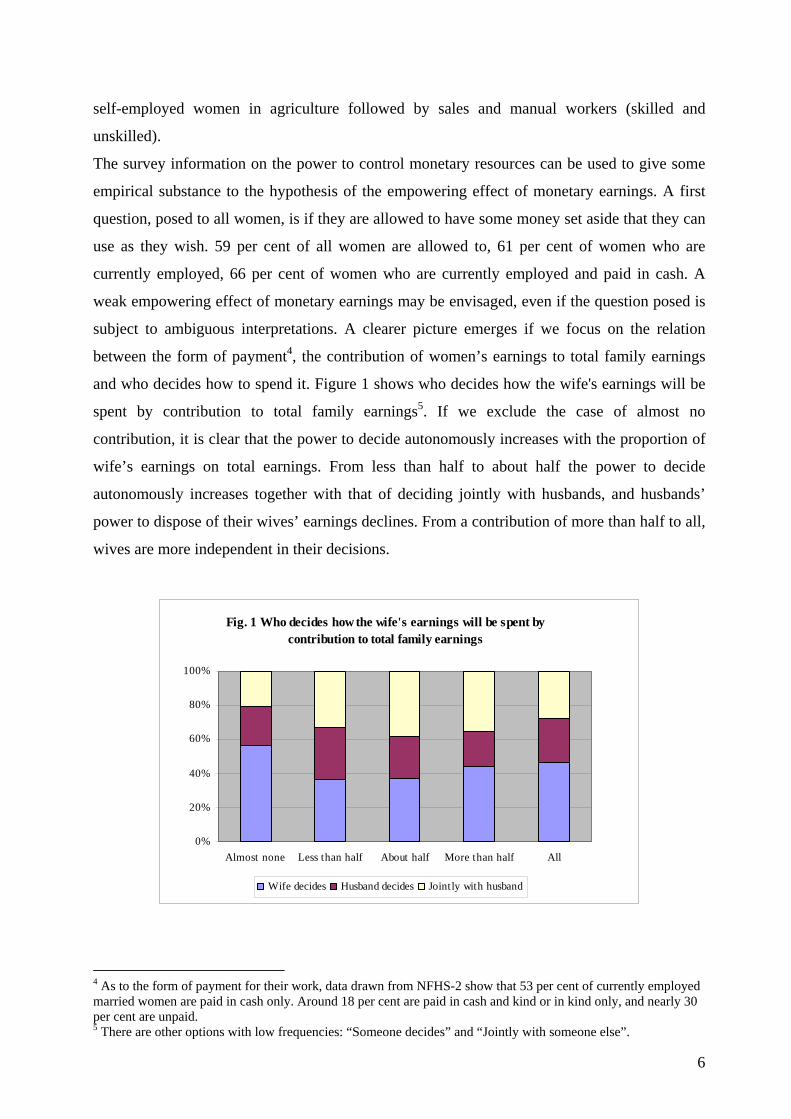
subject to ambiguous interpretations. A clearer picture emerges if we focus on the relation

between the form of payment4, the contribution of women’s earnings to total family earnings

and who decides how to spend it. Figure 1 shows who decides how the wife's earnings will be

spent by contribution to total family earnings5. If we exclude the case of almost no

contribution, it is clear that the power to decide autonomously increases with the proportion of

wife’s earnings on total earnings. From less than half to about half the power to decide

autonomously increases together with that of deciding jointly with husbands, and husbands’

power to dispose of their wives’ earnings declines. From a contribution of more than half to all,

wives are more independent in their decisions.

Fig. 1 Who decides how the wife's earnings will be spent by contribution to total family earnings

0%

20%

40%

60%

80%

100%

Almost none Less than half About half More than half All

Wife decides Husband decides Jointly with husband

4 As to the form of payment for their work, data drawn from NFHS-2 show that 53 per cent of currently employed married women are paid in cash only. Around 18 per cent are paid in cash and kind or in kind only, and nearly 30 per cent are unpaid. 5 There are other options with low frequencies: “Someone decides” and “Jointly with someone else”.

6

3 Governmental Programmes for economic development and

employment (GP)

Programmes to easy the access to employment have been implemented in India since the 80s6.

Some of these were specifically addressed to women with the aim of promoting stable and paid

occupations. The National Population Policy adopted by the Government of India in 2000

(Ministry of Health and Family Welfare, 2000) explicitly recognized the importance of

women’s paid employment in achieving the goal of population stabilization and specified

measures for paid employment and self-employment. Since women’s participation in rural

areas is higher, policy makers have traditionally concentrated there their intervention with the

objective of improving female work conditions.

Public programmes for economic development aim at alleviating rural poverty through the

endowment of productive assets or skills that the poor can employ to increase their labour

earnings and thus cross the poverty line. The main one is the Integrated Rural Development

Programme (IRDP) started in the 80s. Some of these programmes have a female target. For

example, the Development of Women and Children of Rural Areas (DWCRA), a sub-scheme

of IRDP started in 1982-83, provides opportunities of self-employment for female members of

the rural families below the poverty line7. TRYSEM (Training of Rural Youths for Self

Employment) is a specifically employment oriented programme under the more general

Employment Guarantee Scheme (EGS).

Since 1985-86 two schemes were implemented under the Rural Landless Employment

Guarantee Programme (RLEGP): the first one is the Sanjay Gandhi Niradhar Yojana (SGNY),

with the objective of providing houses free of cost to the houseless families of rural, hilly and

slum areas; the second one is the Indira Awaas Yojana (IAY), with the objective of providing

grant for construction of houses to members of Scheduled Castes/Scheduled Tribes, to freed

bonded labourers and also to rural poor below the poverty line.

The NFHS-2 collects information on each of these programmes at a village level, recording the

number of people in the village who benefited from each one of them in the year preceding the

survey. The most widely available rural development programmes, as reported by the

6 For a discussion of employment programmes in India see Mahendra (2006) 7 Another policy relevant for women empowerment is the 1993 amendment to the constitution of India that requires that the States reserve one-third of al1 positions of chief village to women. Chattopadhyay and Duflo, (2004) show that reservation affects policy decisions in ways that seem to better reflect women's preferences. For example, women complain more often than men about drinking water than about roads. In villages headed by women there are more investments in water and less investment in roads.

7

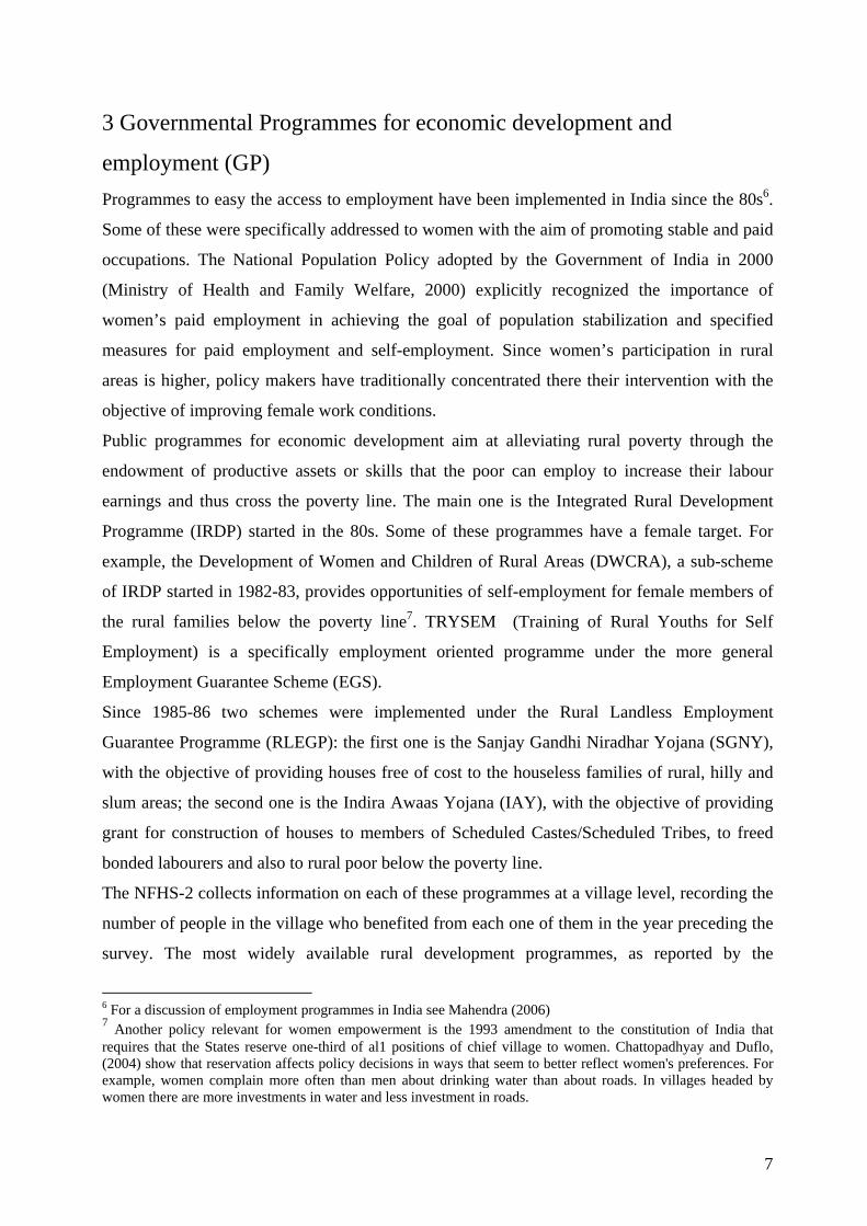
respondents to the Village Questionnaire, are the IAY and the IRDP. DWCRA, the programme

with a female target, covers 23 per cent of total population.

Table 1: Income support and Labour Market Programmes for Rural Development. Percentage of beneficiaries over total de jure popolation Category Acronyms Percentage Integrated Rural Development Programme

IRDP 55.9 Development of Women and Children of Rural Areas DWCRA 23.1

Employment Guarantee Scheme EGS 9.5 National Rural Employment Programme NREP 12.4 Training of Rural Youths for Self Employment TRYSEM 8.9 Sanjay Gandhi Niradhar Yojana SGNY 11.7 Indira Awas Yojana IAY 61.5 Source: NFHS-2, 1998-99

4 The Family Planning programme (FP). As to demographic policies, women aged 15 to 49 are the specific target of Family Planning

programmes (FP). Even if the main objective of FP programmes is demographic, indirect

effects on women’s economic conditions through maternal and child health improvements are

surely to be expected.

The FP Programme8 in India has undergone important changes in recent years and particularly

during the 1990s. At the beginning in 1952, it was primarily a clinic-based family planning

programme monitoring the family on the basis of family planning targets to achieve a couple

participation rate to the health system of 60 percent. After the adoption of the “extension

approach” in 1963 and subsequent integrations with the maternal and child health programme,

the activities of the programme broadened significantly. In addition to family planning, the

programme provided a variety of services to mothers and children, including antenatal,

delivery, and postnatal care, immunization of children against various vaccine-preventable

diseases, and counselling on maternal and child health problems and nutrition. In the 70s and

80s the FP programme has been accused of using unacceptable methods to induce people to be

sterilized and to fulfill administrative targets even after the so called “emergency period”

imposed by President Indira Ghandi in 1976-77 (see Saavala, 1999). The central administration

gave local health workers targets for the number of women they were to sterilize each month. 8 The actual name is “Family Welfare Program”. We rename it FP for expositional purposes, in order to make a clear distinction between demographic and economic welfare policies.

8

During the years, the emphasis on achieving method-specific targets, particularly sterilization

targets, has created a situation in which targets for numbers of acceptors gained precedence

over everything else and the programme was not driven by demand.

The International Conference of Population and Development in 1994 in Cairo marked the

abolition of the target-oriented approach. The programme was gradually reoriented towards the

Reproductive and Child Health Programme that includes components relating to sexually

transmitted diseases and reproductive tract infections. After some initial experiments in a few

selected districts, in 1996 the “target-free” approach was implemented throughout the country

and was renamed the Community Needs Assessment. This approach modified the system of

monitoring the programme and made it a demand-driven system in which a worker would

assess the needs of the community at the beginning of each year. From then on, FP workers are

sent in rural areas to assess the needs of the village communities on the basis of consultations

with families, and give advice on a series of problems, not only concerning health (Ministry of

Health and Family Welfare, 1998b).

The NFHS includes several questions on the quality of care, of health and family welfare

services provided by the public sector and the private sector. The success of FP programmes in

our period of analysis is particularly evident in States with demographic and social indicators

below the Indian average. Taking as an example one of the most underdeveloped States, Uttar

Pradesh, in 20059, 53 per cent of women aged 20-24 were married by age 18, an indicator that

was equal to 64 percent in 1999. In the same period, the total fertility rate has dropped from

4.06 to 3.82 and the median age at first birth has increased from 18.8 to 19.4 years. The

percentage of married women with two living children wanting no more children has risen

from 45 to 64. As far as maternal and reproductive health is concerned, antenatal care has

increased from 35 to 67 percent of births in the preceding three years, 29 to 64 in rural areas.

This fact, together with the increase in institutional deliveries has led to a decrease in infant

mortality from 89 to 73 per 1000 births in the past five years.

The FP Programme in India is still being reformed. The recent National Population Policy,

released in February 2000, stresses the commitment to reproductive and child health with the

statement that “the overriding objective of economic and social development is to improve the

quality of lives that people lead, to enhance their well-being, and to provide them with

opportunities and choices to become productive assets in society” (Ministry of Health and

Family Welfare, 2000).

9 This statistics are drawn from some preliminary reports available for selected States of the new survey NFHS-3 held in 2005-06. The micro-data have not been released yet.

9

5 A baseline theoretical model We fit our model to the issue of women’s empowerment in developing countries. We use a

household model with home production, where decision-making is in the hands of two

partners10. We adopt a “collective approach”11, according to which the two partners have two

distinct utility functions, Ui(.), with i=1,2, that they maximize as a weighted average with

weights representing the balance of power in the household. Since our focus is on female

participation in the labour market, we assume that men always work in the market12, the

partners consume a bundle of domestic (Xd) and market (Xm) goods, and the woman has to

allocate her time between hours of domestic activities, Hd, market work, Hm, and leisure, L. We

identify domestic work with time spent providing food and preparing meals, preventing and

curing diseases of all the family members, and time spent looking after children.

The woman (1) and the man (2) value the two goods in the same way, but the woman has also

her leisure L in her utility function. Man’s leisure is assumed to be zero. The husband is only

indirectly interested in his wife’s time, since the household needs to consume at least a

minimum level of domestic goods, which he is not able to produce himself being specialized in

market labour13.

Under these hypotheses the household utility to be maximized is simply:

Max U= UΘ 1(X,L)+ (1-Θ )U2(X) (1)

where 0<Θ <1 is a coefficient that is positively related to the power of the wife14.

To begin with, imagine a situation of underdevelopment where women are forced to allocate all

their time to domestic work. To give an example, suppose that a couple is not able to control

fertility, that health of the household members is at continuous risk, that water and food is

difficult to provide and to transform in safe drinks and meals. In one word, home production

technology is very poor. As a result, the woman will be overridden by domestic tasks, and all

10 See, for example, Cigno (1991), ch. 2. 11 See the literature started by Bourguignon and Chiappori (1992). For an extensive survey, see del Boca and Flinn (2005). 12 This is a realistic assumption. In our sample drawn from NFHS-2, 97% of husbands work. 13 Browning and Gortz (2006) call this the “no externalities” assumption, that allows to decentralise any allocation by a redistribution of initial endowments (see p.14). Alternatively, it can be assumed that L enters directly the husband’s utility function, like in Basu (2006), if he draws utility from his wife’s leisure. Even if this goes beyond the scope of our empirical analysis, we shall return to it later. 14 Browning and Gortz (2006) call this the “Pareto weight”, that may depend on observables such as relative wages and extra-household factors and unobservables such as the degree of caring and personalities of the two partners.

10

her time will just be sufficient to provide her family and herself the means to survive. The man

gives the household a labour income Y, used to buy market goods. We call this period 1.

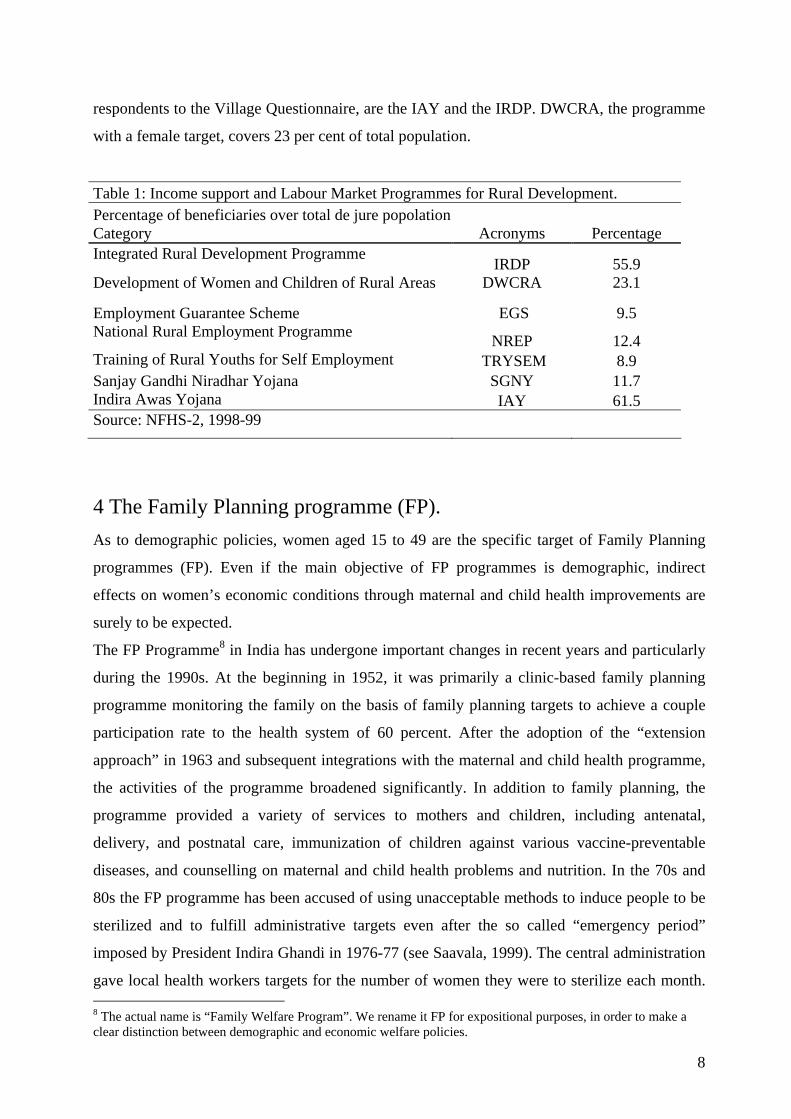
Period 1: no choice

In period 1, a woman in the household has no choice over the way she can use her time. She

has to produce a given minimum amount of domestic goods, Xd,min, for her and her family

survival. This activity will take all her time T, she will have no alternative, and her power will

be null, that is . Hence, in the beginning the household preference coincides with the

husband’s preference. If X

0=Θ

d = f(Hd) is the domestic production function, we assume that at time

1 the wife will have to produce survival Xd,min=f(T). The household will consume also some

market goods, that is Xm =Y (see Fig. 2).

Suppose the government decides to intervene to improve households’ welfare with a family

planning policy that sends family planning workers to visit families and give them advice on

health, fertility, child care and other related matters. This implies a sudden improvement in

domestic technology that gives the woman an opportunity to employ her time resources more

efficiently, and, by consequence, a certain degree of control over them. We call this period 2.

X

Xd,min

LT

g(Hd)2f(Hd)1

Hd,2

Hd,1

w

A

Hd,min,2

Fig. 2 Domestic technology improvement after an exogenous shock:From the no choice case (1) to the non-participation decision (2)

Y=Xm

11

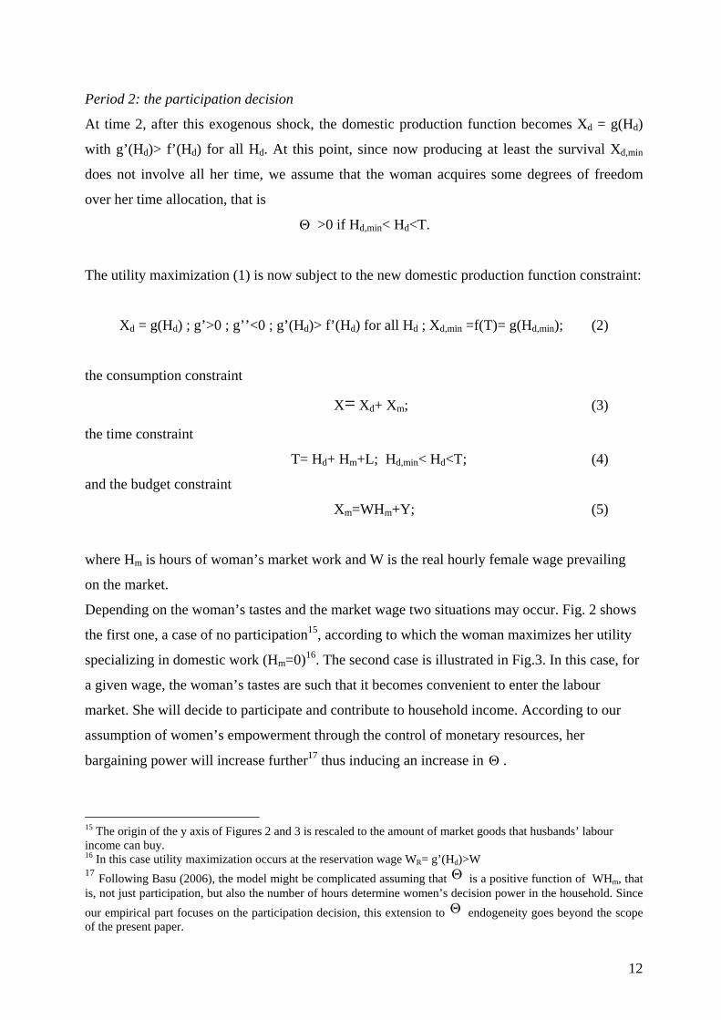
Period 2: the participation decision

At time 2, after this exogenous shock, the domestic production function becomes Xd = g(Hd)

with g’(Hd)> f’(Hd) for all Hd. At this point, since now producing at least the survival Xd,min

does not involve all her time, we assume that the woman acquires some degrees of freedom

over her time allocation, that is

Θ >0 if Hd,min< Hd<T.

The utility maximization (1) is now subject to the new domestic production function constraint:

Xd = g(Hd) ; g’>0 ; g’’<0 ; g’(Hd)> f’(Hd) for all Hd ; Xd,min =f(T)= g(Hd,min); (2)

the consumption constraint

X= Xd+ Xm; (3)

the time constraint

T= Hd+ Hm+L; Hd,min< Hd<T ; (4)

and the budget constraint

Xm=WHm+Y; (5)

where Hm is hours of woman’s market work and W is the real hourly female wage prevailing

on the market.

Depending on the woman’s tastes and the market wage two situations may occur. Fig. 2 shows

the first one, a case of no participation15, according to which the woman maximizes her utility

specializing in domestic work (Hm=0)16. The second case is illustrated in Fig.3. In this case, for

a given wage, the woman’s tastes are such that it becomes convenient to enter the labour

market. She will decide to participate and contribute to household income. According to our

assumption of women’s empowerment through the control of monetary resources, her

bargaining power will increase further17 thus inducing an increase in Θ .

15 The origin of the y axis of Figures 2 and 3 is rescaled to the amount of market goods that husbands’ labour income can buy. 16 In this case utility maximization occurs at the reservation wage WR= g’(Hd)>W 17 Following Basu (2006), the model might be complicated assuming that Θ is a positive function of WHm, that is, not just participation, but also the number of hours determine women’s decision power in the household. Since our empirical part focuses on the participation decision, this extension to Θ endogeneity goes beyond the scope of the present paper.

12

X

Xd,min

LT

g(Hd)2

f(Hd)1

Hm,2

Hd,2

Hd,1

w

A

Hd,min,2

Fig. 3 Domestic technology improvement after an exogenous shock:From the no choice case (1) to the participation decision (2)

Y=Xm

B

dXm

The first order conditions of the maximization of U(.)1 with respect to Hm and Hd are:

WUU

X

L = (6)

and

)(' DX

L HgUU

= (7)

where (6) corresponds to Pareto efficiency in the consumption allocation. From (6) and (7) the

equilibrium condition of equality of the marginal product of household production and the

wage rate18 is derived.

18 Supposing the price of Xm equals unity, then in monetary terms (6) and (7) yield , that is, in equilibrium, the revenue of an extra hour of domestic work must equal its marginal cost. This relation is useful to impute a price p

)('*DHgpw =

* to domestic input in empirical work when time use data are available (see Apps and Rees, 1997).

13

For empirical purposes, we adopt a static utility comparison framework. In this theoretical

context, the woman works if the indirect utility of working for the market is greater than the

indirect utility derived from specializing in domestic work. We want to measure how much of

the outcome will depend on the exogenous change in domestic technology and in the woman’s

bargaining power. If the effect will be such to override the threshold given by her reservation

wage, she will maximise her utility working outside home.

In other words we assume her indirect utilities to be:

vwork (W,Y, Θ ) ,vnot work(W,Y, Θ )

Since our data do not contain information on wages and incomes, we are compelled to use a

reduced form specification. W will depend on the usual set I of individual characteristics of the

woman such as age and education, Y will depend on her partner’s characteristics P, including

education and position in the labour market, Θ will depend on some indicators of public

policies that improve domestic technology and the employment probability (FP and GP). The

participation decision will also be affected by other observable household variables H, such as

the number and age of children, the household size, and wealth. The above assumptions imply

that each indirect utility depends on the following set of variables:

v=v( I, P, H, FP, GP)

In conclusion, to observe a woman working, for example, means that:

max(vwork, vnot work)= v*work.

The empirical part will focus on the following testable predictions that:

1) the participation decision is significantly affected by domestic productivity enhancing

demographic policies (FP);

2) the participation decision is significantly affected by employment policies (GP);

3) demographic policies have an impact on the employment probability of women that is

at least as large as that of governmental economic programmes.

14

6 Data and variables

The micro data we use are drawn from the National Health Family Survey19, 1998-1999

(NFHS-2). This survey20 is designed to provide state and national estimates of fertility, the

practice of family planning, infant and child mortality, maternal and child health, and the

utilization of health services provided to mothers and children. In addition, the survey provides

indicators of the quality of health and family welfare services, women’s reproductive health

problems, and domestic violence, and includes information on the status of women, education,

work and standard of living.

The NFHS-2 is a household survey with a sample size of around 92,500 households and 90,300

ever-married women in the age group 15–49. The sample covers more than 99 percent of

India’s population living in all 26 Indian states.

The sample size for each state was drawn separately for urban and rural samples proportionally

to the size of the state’s urban and rural populations21. In all states a uniform sample design

different for rural and urban areas was adopted. For the creation of the rural sample a two sages

procedure was adopted: in the first stage some villages were selected as Primary Sampling

Units (PSUs) following a PPS approach (probability to be selected proportional to population

size); in the second stage households were randomly selected within each PSU. In urban areas,

a three-stage procedure was followed. In the first stage wards were selected with PPS sampling,

in the second step from each sample ward one Census Enumeration Block (CEB) was

randomly selected, and in the third stage households were randomly selected within each

sample CEB. On average, 30 households were initially targeted for selection in each selected

enumeration area

NFHS-2 used three types of questionnaires: the Household Questionnaire, the Woman’s

Questionnaire, and the Village Questionnaire. The Household Questionnaire listed all usual

residents in each sample household plus any visitors who stayed in the household the night

before the interview. For each listed person in the household, the survey collected basic

information on the relationship to the household head and age, sex, marital status, religion,

caste/tribe, education, and occupation. The Household Questionnaire also collected information

on indicators of household well-being such as the main source of drinking water, type of toilet

facility, source of lighting, type of cooking fuel, ownership of house, ownership of agricultural 19 The data are supplied by ORC Macro, Maryland, US. 20 The first survey was conducted in 1992-93, before the introduction of the FP programme we focus on. 21The 1991 Census list of villages served as the sampling frame for rural areas. The 1991 Census list of wards served as the sampling frame for urban areas.

15

land, ownership of livestock, and ownership of other selected items. In addition, the household

questionnaire included very detailed information on household members’ health.

Information on age, sex, and marital status of household members was used to identify eligible

respondents for the Woman’s Questionnaire. Eligible women for the Woman’s Questionnaire

are defined as all ever-married women aged 15–49 who were usual residents of the sample

household or visitors who stayed in the sample household the night before the interview. The

Women’s Questionnaire collected information on the following topics: background

characteristics, reproductive behaviour and intentions, quality of care, sources of family

planning, antenatal, delivery, and postpartum care, breastfeeding and reproductive health,

knowledge of AIDS. Woman’s Questionnaire also investigated on the status of women in the

household asking about the treatment of women in the household, gender roles, women’s

autonomy and violence against women. Questions are also asked about women’s husbands.

The Village Questionnaire collected information from the sarpanch (village head), other

village officials, or other knowledgeable person in the village on the availability of various

facilities and services in the village (such as health and education facilities, electricity and

telephone connections, and others). One important set of questions regarded the distance of the

village from various types of facilities including Primary Health Centres, sub centres, hospitals,

and dispensaries or clinics and the presence in the villages of services like schools (of different

levels) and anganwadi (a nursery school for children age 3–6 years). The Village Questionnaire

also collected information about development and welfare programmes operating in the village.

Among eligible women we select only married women that amount to a sample of around

85000 observations. This is standard practice in the literature on female participation in the

developed world, under the assumption that married women have utility functions and budget

constraints different from the no more married and the never married single women, who

behave similarly to their male counterpart. The NFHS sample does not include never married

single women, but only the no more married group formed by widowed, divorced and deserted

women. It is anyway necessary to select them out, since this group is traditionally worlds apart

from the married women group22. The sample includes married women with and without

children, since the latter represent a target of FP visit as potential mothers.

The dataset we construct includes relevant information collected from the Woman

Questionnaire supplemented with information at a household level and, for rural India, at a

22 Being no more married is a negative social stigma. In some rural areas of India, it is a common situation that if a husband dies, his widow is considered guilty. In some of the most underdeveloped parts of rural India, if the widow hasn't got a son, the people think that she must die too, because she is useless. The law punishes severely the “Sati”, a ferocious ceremony where a widow, usually very young, is burned alive.

16

village level. The dataset includes, together with women’s background characteristics,

information on the dimension and composition of the household, on other household’s

components, including occupation and household wealth23. Moreover, our data set contains

detailed information on family planning services provided to the household and, at a village

level, on the coverage of governmental programmes for economic development of rural areas.

6.1 Definition of the dependent variable In order to contribute to assessing female labour market conditions in developing countries, we

construct three variables of female employment probability.

The first one is a binary dependent variable based on the question “Are you currently

employed?” We concentrate our analysis on women who are currently employed because we

observe that only a low percentage of women (less than 3 per cent, mostly seasonal workers)

was working during the year but was not currently working. About 33 per cent of married

women is currently employed at the time of interview.

As we assume that the empowerment process speeds up increasing the control over monetary

resources, the state of being employed does not necessarily improve women’s condition, since

a large share of female workers is unpaid. Only 62 per cent of the employed women of our

sample are paid in cash, whereas the others are unpaid. Our second dependent variable,

therefore, is a multinomial variable with three states, not working, working unpaid and working

paid.

A further distinction is related to the duration of work. Permanent jobs are more probably

related to women’s empowerment. A distinction between “all year” and “occasional” activities

is therefore necessary, since a high percentage of employed women (more than 33 per cent)

does not work all the year, but is engaged in seasonal or occasional activities. In other words,

we divide the better off category of paid workers in those who are engaged in seasonal or

occasional activities and those who are employed all year. Thus, the third specification is a

23 The selection of indicator variables to be included in the wealth index is relatively straightforward. Almost all household assets and utility services are to be included, including country-specific items. The reason for using a broad criterion rather than selected items is that the greater the number of indicator variables, the better the distribution of households with fewer households being concentrated on certain index scores. Generally, any item that will reflect economic status is used. Two additional indicators are considered: whether there is a domestic servant and whether the household owns agricultural land. The first is constructed by examining the occupation of interviewed members who are not related to the head of the household. If the respondent or spouse works as a domestic servant and is not related to the head, then the household is considered to have a domestic servant. The second is also based on interviewed members. If any interviewed member (related to the head or not) or interviewed member’s spouse works his or her own or his or her family’s land, then the household is considered to own agricultural land (Rutstein and Johnson, 2004, p.17).

17

multinomial variable with four states: no work, work unpaid, seasonal work paid, all year work

paid.

Looking at the distinction between urban and rural areas, we observe that the percentage of

women at work is higher in rural areas (39 percent against 22 percent). In rural areas it is also

more likely to work as unpaid workers or to be paid in kind (56 percent in rural areas against 12

percent in urban areas) and to be employed seasonally (36 percent in rural areas against 22

percent in urban areas).

6.2 Constructing exogenous FP indicators and comparable GP variables Having assessed the relevance of FP in relaxing the burden of women’s reproductive and health

care roles, we ask whether there is any evidence of a positive impact of these programmes on

women’s position in the labour market. Using the survey micro data for all Indian States, we

focus on the relation between FP programmes and women’s employment probability.

Information on FP comes form the women’s questionnaire.

The survey provides information on many aspects of the FP intervention, like, for example, the

use of health facilities. We do not use these demand driven indicators, since they would be

endogenous to women’s choices. Instead, exploiting the fact that differentials in home visits by

background characteristics are generally small, we use, as indicators of the exposition to FP

programmes, the passive event of having received at least one visit from an FP worker in the

previous twelve months. This indicator should be exogenous to women’s choices, depending

on the coverage strategy of each State. 13 percent of women aged 15-49 received at least one

visit (and, among them, three visits on average24) which is an impressing result considering the

huge Indian population. During these contacts the FP workers monitor various aspects of the

health of women and children, provide information related to health and family planning and to

the supply of public services, counsel and motivate women to adopt appropriate health and

family planning practices. We construct a dummy variable (FPVISIT) which equals one if a

women has received a visit in the last 12 months.

Once measured the impact of FPVISIT on the probability of being employed, we then want to

compare this effect with that of GP. These variables, recording income support and labour

policies, are collected within the village questionnaire, where a village head (sarpanch) is

asked about the number of persons in the village receiving a specific benefit. To make the

comparison we transform FPVISIT in two new variables. The first one takes value one if a 24 The number of FP visits per woman, instead, might be endogenous if the woman asks the FP worker to visit her again. We therefore do not use this variable.

18

woman lives in a village where an FP worker has visited at least one woman (even if not

herself).

To compare coefficients, we also build a dummy for each welfare programme with the same

criterion, that is the programme dummy takes value one if a woman lives in a village where

there is at least one beneficiary of the program. The second variable is the ratio of the number

of women who received a visit in the village over the total number of people in the village

sample. This ratio is based on the sample values representative of the village-universe. For the

GP variables we build the ratio of the effective number of people in the village who benefited

from each specific programme over the village de jure25 population.

7 Results We estimate logit and multinomial logit specifications of women’s employment probability for

all States of India, distinguishing between urban and rural India (see the Appendix for the

descriptive statistics of all the variables used in the model). For rural India, we also conduct a

separate analysis exploiting the additional village information. As we have seen in the data

section, for rural India the NFHS provides variables on the number of beneficiaries of a set of

governmental programmes whose effects we want to compare with those of FP programmes26.

We first present our results on the impact on participation of FPVISIT for all India. We then

compare the impact of FP with that of GP in rural India.

7.1 The employment probability and FP

We start with the impact of FP, and then compare it with that of other control variables that

contribute to determine women’s participation according to well-established theory and

empirical observation. Table 2 reports the marginal effect of FPVISIT on the probability of

working of married women aged 15-49 in all Indian States.

25 Residing population. 26 The NFHS-2 Village Questionnaire collected information from the sarpanch, other village officials, or other knowledgeable persons in the village on facilities and services in the village that can affect health and family planning. One important set of questions focuses on the distance of the village from various types of health facilities, the presence in the village of schooling facilities, including nurseries (angawadi).

19

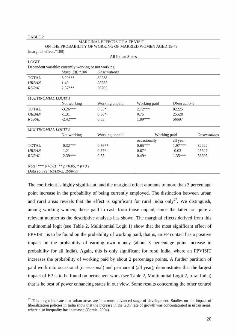
TABLE 2 MARGINAL EFFECTS OF A FP VISIT

ON THE PROBABILITY OF WORKING OF MARRIED WOMEN AGED 15-49 (marginal effects*100)

All Indian States LOGIT Dependent variable: currently working or not working Marg. Eff. *100 Observations TOTAL 3.29*** 82238 URBAN 1.40 25533 RURAL 2.57*** 56705 MULTINOMIAL LOGIT 1 Not working Working unpaid Working paid Observations TOTAL -3.26*** 0.55* 2.72*** 82225 URBAN -1.31 0.56* 0.75 25528 RURAL -2.42*** 0.53 1.89*** 56697 MULTINOMIAL LOGIT 2 Not working Working unpaid Working paid Observations occasionally all year TOTAL -0.32*** 0.56** 0.65*** 1.97*** 82222 URBAN -1.21 0.57* 0.67* -0.03 25527 RURAL -2.39*** 0.55 0.49* 1.35*** 56695 Note: *** p<0.01, ** p<0.05, * p<0.1 Data source: NFHS-2, 1998-99

The coefficient is highly significant, and the marginal effect amounts to more than 3 percentage

point increase in the probability of being currently employed. The distinction between urban

and rural areas reveals that the effect is significant for rural India only27. We distinguish,

among working women, those paid in cash from those unpaid, since the latter are quite a

relevant number as the descriptive analysis has shown. The marginal effects derived from this

multinomial logit (see Table 2, Multinomial Logit 1) show that the most significant effect of

FPVISIT is to be found on the probability of working paid, that is, an FP contact has a positive

impact on the probability of earning own money (about 3 percentage point increase in

probability for all India). Again, this is only significant for rural India, where an FPVISIT

increases the probability of working paid by about 2 percentage points. A further partition of

paid work into occasional (or seasonal) and permanent (all year), demonstrates that the largest

impact of FP is to be found on permanent work (see Table 2, Multinomial Logit 2, rural India)

that is he best of power enhancing states in our view. Some results concerning the other control

27 This might indicate that urban areas are in a more advanced stage of development. Studies on the impact of liberalization policies in India show that the increase in the GDP rate of growth was concentatrated in urban areas, where also inequality has increased (Cornia, 2004).

20

variables (see Table 3) are worth commenting for the differences in labour conditions with

respect to developed countries (see the Appendix for the complete model specification).

TABLE 3 MARGINAL EFFECTS OF WOMEN'S EDUCATION AND OF FAMILY CHARACTERISTICS (marginal effects*100) All Indian States TOTAL URBAN RURAL Education Womans's years of education -4.39*** -2.71*** -4.55*** Womans's years of education sq. 0.37*** 0.26*** 0.34*** Children in the household Own children aged 0-2 -6.66*** -5.12*** -7.25*** Own children aged 3-5 0.24 -0.08 0.33 Own children aged 6-14 1.07*** 0.92*** 0.94*** Other children in the family aged 0-2 0.29 0.06 0.27 Other children in the family aged 3-5 0.33 2.25*** -0.39 Other children in the family aged 6-14 0.55* 1.07** 0.20 Husband's employment position Professional -2.00* -3.65** -0.801 Salesman -8.15*** -8.40*** -7.54*** Self-employed in agriculture 3.86*** 2.06 4.72*** Skilled blue collar -5.65*** -6.59*** -4.08*** Unskilled blue collar -8.39*** -4.45*** -9.40*** Wealth index -10.5*** -8.49*** -11.7*** Note: *** p<0.01, ** p<0.05, * p<0.1 Data source: NFHS-2, 1998-99

As far as schooling is concerned, female employment is negatively correlated with years of

education, with a higher negative effect in rural areas. Mahendra (2004) uses the Household

sample of the NFHS-2 survey to study the association of female work participation with the

level of schooling. His sample is larger than ours, including all women (married and unmarried,

with children and without) aged 15-5928. The negative relation with schooling is confirmed in

rural areas, but he finds a positive, but much less significant, association in urban areas. This

result might be due to the presence of young unmarried women without children and older

women with adult children. For our sample of married women 15-49 drawn from the Women’s

sample (therefore less numerous) the association remains negative in urban areas as well, but

the marginal effect is lower than in rural areas. This is a major difference with married women

participation in developing countries, where education has always been considered as the

primary condition to achieve autonomy. Our result rejects this hypothesis for Indian mothers, 28 The author, however, does not control for the presence of children and other household composition variables.

21

thus suggesting other important roles of mothers’ education in Asian societies, such as

improving children’s welfare and education (Behrman, Foster, Rosenzweig and Vashishtha,

1999). Several studies failed to find evidence of a positive link between women's education and

female autonomy, casting doubt on one of the major pathways through which the former was

supposed to reduce fertility (see, for example, Jeffery and Basu, 1996, Jeffery and Jeffery,

1996)29. No doubt the role of education for development is fundamental. Various studies have

shown the positive effect of maternal education on child health and survival (among these,

Dreze and Murthi, 2001). Analyzing data of NFHS-1, 1992-93, Govindasamy and Ramesh

(1997) found that mother’s education continues to be a powerful, positive and significant

predictor of utilization of child health care services in India, even after controlling for a number

of other demographic, socioeconomic and spatial variables. Mothers’ education is also found to

reduce the gender discriminatory practices among mothers of children seeking medical

treatment during the post-neonatal and later childhood period (Ghosh, 2004, on NFHS-2).

Turning to the impact of the presence of children in the household, the effect of the number of

woman’s small children is negative, but only of children up to the age of two; children aged 3

to 5 do not influence their mothers’ employment state, whereas older children have a positive

impact. The negative effect of small children, however, is relatively small (minus 6 percentage

points) as compared to that of FPVISIT (plus 3 percentage points, see Table 2) and to the effect

generally emerging from studies on developed countries. The result that children from 3 to 5 do

not impede women’s work could also be explained by the fact that more than two-thirds of

rural residents live in villages that have an anganwadi (a nursery school for children aged 3 to

6)30. The presence of older children (6-14) has a positive impact on women’s occupation (one

percentage point increase) since they might offer a substantial contribution to household work.

Indian households are often composed by more than one family nucleus. 34 per cent of all

households of the survey belong to this category31. It is therefore reasonable to ask if the

employment status of a woman in a multi-nuclear household depends not only on her own

children, but also on other women’s children residing in the same household. In order to test for

the hypothesis that all children present in the household may have an impact on each residing

woman’s employment we have introduced some variables measuring the number of children of

mothers other than the interviewed. Our test rejects this hypothesis, indicating that only own

29 Dreze and Murthi (2000), however, find strong empirical support to the negative association between education and fertility in India. 30 See the NFHS report 1998/9, chapter 2 p. 46 and also the next paragraph. 31 Nuclear family households consists of an unmarried adult living alone or a married person or a couple and their unmarried children, if any.

22

children matter for women’s choices. Since only own children 0-2 impede entry into the labour

market, the reason is probably to be found in breast-feeding. Nursery services for own children

3 to 5 are therefore not produced within the household by women other than mothers, but most

probably purchased in outside nurseries.

Husbands’ professional position should capture the effect of partner’s income. In fact, all types

of husband’s employment positions reduce a woman’s probability of working, in line with the

evidence for many developed countries like the South European ones. Only one husband state

has a positive impact, that of a husband self-employed in agriculture, with the obvious

implication that wives are involved in the family farm activity.

The coefficient of the wealth index32 is negative, large and highly significant, thus confirming

the stylised fact that in Asian societies wealthier households keep women at home.

7.2 Comparing the impact on women’s employment of FP with that of

GP in rural India

We now compare the FP effect with that of GP, with a particular attention to policies

promoting female employment.

Table 4 and 5 report the marginal effects of FP and of GP on women’s employment probability.

As explained in the data section, we have constructed two new FP variables for comparison

purposes. FPVISIT now has two different meanings: a dummy, taking value one if the woman

lives in a village where there has been at least one visit of a FP worker, and a percentage of the

number of women visited by FP workers over the total village population. The GP variables are

constructed in the same way, so that the coefficients are comparable. The tables report also the

marginal effects of the dummies for the presence of nurseries (anganwadi) and primary

schools, since these are public facilities relevant for women’s employment. It is interesting to

note that anganwadi workers not only provide child care services but also engage in the

promotion of family planning among parents of preschool age children33. The results of the

32 According to Filmer and Pritchett (2001) the principal components analysis is used to assign the indicator weights. This procedure first standardizes the indicator variables (calculating z-scores) and then calculates the factor coefficient scores (factor loadings). Finally, for each household, the indicator values are multiplied by the loadings and summed to produce the household’s index value. In this process, only the first of the factors produced is used to represent the wealth index. The resulting sum is itself a standardized score with a mean of zero and a standard deviation of one. The wealth index does not produce results that are comparable to either an income-or expenditure-based index since it takes into account almost all household assets and utility services. 33 That’s why we have renamed the variable in Table 4 “Nursery and FP centre”. It can not be used with FPVISIT to measure the impact of FP since it might be endogenous to the woman’s employment choice.

23

logit (see Table 4) show that the marginal effect of FPVISIT appears to be relatively high.

Taking the dummy measures (col. 1), FPVIST has the larger marginal effect, increasing the

probability of employment by 5 percentage points, an even larger effect than that shown in

Table 2. This result could be interpreted in this way: a woman that lives in a village where FP

workers have made some visits, benefits from positive externalities due to the diffusion of FP

information even if she has not been contacted personally. This fact increases he effect of

FPVISIT with respect to the variable that took account only of visited women (Table 3).

The presence of facilities for prime age children has the expected positive effect: nursery

facilities, increase the employment probability by around 3 percentage points, thus supporting

our hypothesis of the outsourcing of child care for pre-school children in rural India. The

presence of primary school in the village has also a positive impact, as it is reasonable to

expect.

Turning now to the comparison of the impact of FPVISIT with respect to GP, we find that

some GP have a positive impact and some other have a negative impact on women’s

employment (see Table4 col.1). For example, IRDP (Integrated Rural Employment Program)

TRYSEM (Training of Rural Youth for Self-Employment), NREP (National Rural

Employment Program) have all a negative impact, as if they would support mainly husbands’

employment, thus increasing partner’s income and generating a negative income effect on

participation34.

It is probably for this reason that more specific GP for women’s employment have been

introduced more recently. We find, however, that the effect of one of these, the Development of

Women and Children in Rural Areas (DWCRA), is not significant.

To check this result, we use another specification that take in to account the percentage of

beneficiaries in the village. Since the FPVISIT variables in col. 2 of Table 4 are continuous,

they provide additional information (with respect to the dummy of col. 1) on the dimension of

each programme intervention by village. It is therefore reasonable to expect different relative

magnitudes and significance of the marginal effects with respect to col. 1. In fact, the marginal

effects are no longer larger for FPVISIT and, in particular, the effect of DWCRA becomes

significant and larger than that of FPVISIT. Summing up all the GP marginal effects, the total

impact amounts to 1.45, nearly identical to the coefficient of FPVISIT (1.5). This result

suggests that the total impact of the various GP on women’s employment is just the same as

34 It could also be that if a husband receives a benefit from one programme this makes his wife ineligible for another one. On these aspects, however, we need to investigate further.

24

that of FP, whose effect should be regarded as operating much more indirectly, through the

improvement of domestic production technology.

TABLE 4 COMPARING THE EFFECTS OF FP VISIT WITH GP - LOGIT Dependent variable: work/no work (marginal effects*100) Rural India Dummies Beneficiaries

(% of village population)

(col.1) (col.2) Family Planning FPVISIT 5.54*** 1.50*** Prime age facilities Nursery and FP centre 2.73*** 2.33***+ Primary school in village 3.61*** 3.87***+ GP-Welfare and Labour Market programmes IRDP -1.66** -0.80*** NREP -4.66*** -0.71* TRYSEM -4.31*** -3.70*** EGS 3.26*** 2.02*** DWCRA 0.24 2.61*** IAY 0.54 0.40 SGNY 4.15*** 1.63*** Observations 51754 51740 Note: *** p<0.01, ** p<0.05, * p<0.1; +:dummy Data source: NFHS-2, 1998-99

The problem is that some GP, supporting household incomes and male employment, have a

discouraging effect on women’s participation. Specific female oriented employment measures

just counterbalance these negative outcomes.

In order to assess the role of the different GP for paid and unpaid work, we estimate the

Multinomial logit 1 also for this specification (see Table 5). The specification with the

dummies for the presence of beneficiaries in the village confirms that FPVISIT is significant,

especially for paid work, and DWCRA is not. The specification with beneficiaries in

percentage of village population shows that the effects are very similar for paid and unpaid

work both for FPVISIT and DWCRA. So, in this case, the externality effect is on the state of

working, independently of monetary payment.

25

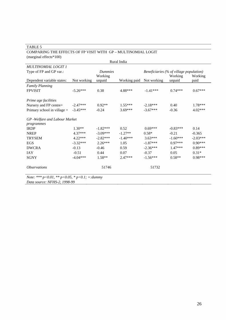
TABLE 5 COMPARING THE EFFECTS OF FP VISIT WITH GP – MULTINOMIAL LOGIT (marginal effects*100)

Rural India MULTINOMIAL LOGIT 1 Type of FP and GP var.: Dummies Beneficiaries (% of village population)

Dependent variable states: Not working Working unpaid Working paid Not working

Working unpaid

Working paid

Family Planning FPVISIT -5.26*** 0.38 4.88*** -1.41*** 0.74*** 0.67*** Prime age facilities Nursery and FP centre+ -2.47*** 0.92** 1.55*** -2.18*** 0.40 1.78*** Primary school in village + -3.45*** -0.24 3.69*** -3.67*** -0.36 4.02*** GP -Welfare and Labour Market programmes IRDP 1.30** -1.82*** 0.52 0.69*** -0.83*** 0.14 NREP 4.37*** -3.09*** -1.27** 0.58* -0.21 -0.365 TRYSEM 4.22*** -2.82*** -1.40*** 3.63*** -1.60*** -2.03*** EGS -3.32*** 2.26*** 1.05 -1.87*** 0.97*** 0.90*** DWCRA -0.13 -0.46 0.59 -2.36*** 1.47*** 0.89*** IAY -0.51 0.44 0.07 -0.37 0.05 0.31* SGNY -4.04*** 1.58** 2.47*** -1.56*** 0.58** 0.98*** Observations 51746 51732 Note: *** p<0.01, ** p<0.05, * p<0.1; +:dummy Data source: NFHS-2, 1998-99

26

8 CONCLUSIONS

Our results support the hypothesis that an exogenous improvement in household production

technology through demographic and health policies has empowering effects on women’s

condition in developing countries. In the first stage of development this improvement is at least

as important for women as that of economic policies sustaining household income and

employment. Our household model in the collective framework predicts that an exogenous

improvement in household production technology gives the wife the opportunity to employ her

time resources more efficiently, and, by consequence, the power to choose to participate or not

to the labour market. If she chooses to participate in paid work, her decision power in the

household will increase further.

Our econometric evidence for India does not reject this hypothesis, showing a positive impact

of an exogenous FP scheme (the family planning worker visit) on women’s employment

probability. Coherently with the hypothesis that the model fits a primitive stage of

development, the effect is significant only for rural India, indicating that in urban areas the

technological improvement in household production has already produced its effects. As to the

empowering feedback of demographic measures, our results show that the largest positive

impact of FP in rural India is to be found on permanent paid work, as opposed to occasional

and unpaid work.

The FP effect is robust to the introduction of income and labour market programmes (GP),

some of them directly targeted to reduce women’s vulnerability problem. Moreover, the

comparison between these programmes shows that their total impact on women’s employment

probability in rural India is just the same as that of FP. The problem is that some GP,

supporting household incomes and male employment, have a discouraging effect on women’s

participation. We find that more specifically female oriented employment measures just

counterbalance these negative outcomes.

If we believe that women’s empowerment is closely related to the earning capacity stemming

from a permanent paid job, the contribution of FP programmes has to be regarded as a

successful, albeit indirect, intervention in this direction. As to public income support and

employment policies, they must be carefully studied with an eye to intra-household dynamics,

in order to avoid disincentive effects on female participation that could counterbalance the

positive effects of specific measures for female employment.

27

References Apps P. F., R. Rees, (1997), “Collective Labor Supply and Household Production”, The Journal of Political Economy, Vol. 105, No. 1, pp. 178-190 Basu, K. (2006), “Gender and Say: A Model of Household Behaviour with Endogenously Determined Balance of Power”, Economic Journal 116, 558-580 Behrman J.R., Foster A. D., Rosenzweig, Vashishtha P. (1999), “Women Schooling, Home Teaching and Economic Growth”, The Journal of Political Economy, Vol. 107, N0 4, 682-714 Bourguignon, F. and P.A. Chiappori (1992), “Collective Models of Household Behavior: An Introduction”, European Economic Review 36, pp. 355-364 Browning M., M. Gørtz (2006), “Spending Time and Money within the Household”, University of Oxford, Department of Economics, Discussion Paper Series, n. 288 Chattopadhyay R. and E. Duflo (2004), “Women as Policy Makers: Evidence from a Randomized Policy Experiment in India”, Econometrica, Vol. 72, No. 5. pp. 1409-1443. Cigno S. (1991), Economics of the Family, Clarendon Press, Oxford Cornia G. A (2004), “Changes in the Distribution of Income over the Last two Decades: Extent, Sources and Possible Causes”, Rivista Italiana degli Economisti n 1. Del Boca D.,. Flinn C. J, (2005) “Modes of Spousal Interaction and the Labor Market Environment”, ChilD Working Paper n. 12 Desai S., Jain D. (1994), “Maternal Employment and Changes in Family Dynamics: the Social context of women’s work in rural India”, Population and Development Review, 115-136 Dreze J., M. Murthi (2001), “Fertility, Education and Development: Evidence for India” Population and Development Review, 27(1): 33-64 Ermisch J., M. Francesconi (2004), “The Effect of Parents’ Employment on Children’s Educational Attainment”, ISER WP, University of Essex Filmer, D. , L. Pritchett (2001), “Estimating wealth effects without expenditure data—or tears: An application to educational enrollments in states of India”, Demography 38(1):115-132. Folbre N. R. (1984), “Market Opportunities, Genetic Endowments and Intrafamily resource Distribution”, American Economic Review, 518-20 Ghosh S. (2004), “Gender Differences in Treatment-seeking behaviour during Common Childhood Illnesses in India: Does Maternal Education Matter?”, 18th European Conference on Modern South Asian Studies University of Lund, Sweden. Govindaswamy P., B.M. Ramesh (1997), “Maternal education and the utilization of maternal and child health services in India”, National family Health survey Subject Report, No.5, Mumbai, International Institute for Population Sciences

28

Haddad L., Hoddinott J., Alderman H. (1997), “Intrahousehold Resource Allocation in Developing Countries”, John Hopkins U.P. Jeffery, R., A. Basu (eds.), (1996), Girls’ Schooling, Women’s Autonomy, and Fertility Change in South Asia (New Delhi: Sage). Jeffery, P and R Jeffery (1996), “What's the Benefit of Being Educated: Women's autonomy and Fertility Outcomes in Bijnor”, in Jeffery and Basu (1996). Mahendra S., (2004), “Female Work Participation and Child Labour: Occupational Data From NFHS”, Economic and Political Weekly, February 14, pp. 736-744 Mahendra S., (2006), “Policies and Programmes for Employment”, Economic and Political Weekly, April 22, pp. 1511-1516 Mehra R., (1997), “Women, Empowerment, and Economic Development”, Annals of the American Academy of Political and Social Science, Vol. 554, pp. 136-149. Raikhy P. S., A. Mehra, (2003) “Changing Structure of Female Workforce in India: An Inter-state Analysis”, Indian Journal of Labour Economics 46(4), pp.999-1008 Ruhm C. J., (2004), “Parental Employment and Child Cognitive Development”, Journal of Human Resources, 155-192 Rutstein S.H., Johnson K. (2004), “DHS Comparative Reports No. 6: The DHS Wealth Index”, ORC Macro Calverton, Maryland USA Saavala M., (1999), “Understanding the Prevalence of Female Sterilization in Rural India”, Studies in Family Planning, 30(4), pp.288-301 United Nations Development Program (1996), Human Development Report 1996

World Bank (1991), World Development Report, OUP

29

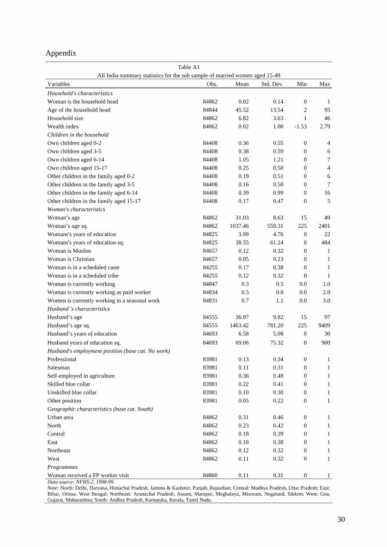
Appendix

Table A1 All India summary statistics for the sub sample of married women aged 15-49

Variables Obs. Mean Std. Dev. Min MaxHousehold's characteristics Woman is the household head 84862 0.02 0.14 0 1Age of the household head 84844 45.52 13.54 2 95Household size 84862 6.82 3.63 1 46Wealth index 84862 0.02 1.00 -1.53 2.79Children in the household Own children aged 0-2 84408 0.36 0.55 0 4Own children aged 3-5 84408 0.38 0.59 0 6Own children aged 6-14 84408 1.05 1.21 0 7Own children aged 15-17 84408 0.25 0.50 0 4Other children in the family aged 0-2 84408 0.19 0.51 0 6Other children in the family aged 3-5 84408 0.16 0.50 0 7Other children in the family aged 6-14 84408 0.39 0.99 0 16Other children in the family aged 15-17 84408 0.17 0.47 0 5Woman's characteristics Woman’s age 84862 31.03 8.63 15 49Woman’s age sq. 84862 1037.46 559.31 225 2401Womans's years of education 84825 3.99 4.76 0 22Womans's years of education sq. 84825 38.55 61.24 0 484Woman is Muslim 84657 0.12 0.32 0 1Woman is Christian 84657 0.05 0.23 0 1Woman is in a scheduled caste 84255 0.17 0.38 0 1Woman is in a scheduled tribe 84255 0.12 0.32 0 1Woman is currently working 84847 0.3 0.5 0.0 1.0Woman is currently working as paid worker 84834 0.5 0.8 0.0 2.0Women is currently working in a seasonal work 84831 0.7 1.1 0.0 3.0Husband 's characteristics Husband’s age 84555 36.97 9.82 15 97Husband’s age sq. 84555 1463.42 781.20 225 9409Husband’s years of education 84693 6.58 5.08 0 30Husband years of education sq. 84693 69.06 75.32 0 900Husband's employment position (base cat. No work) Professional 83981 0.13 0.34 0 1Salesman 83981 0.11 0.31 0 1Self-employed in agriculture 83981 0.36 0.48 0 1Skilled blue collar 83981 0.22 0.41 0 1Unskilled blue collar 83981 0.10 0.30 0 1Other position 83981 0.05 0.22 0 1Geographic characteristics (base cat. South) Urban area 84862 0.31 0.46 0 1North 84862 0.23 0.42 0 1Central 84862 0.18 0.39 0 1East 84862 0.18 0.38 0 1Northeast 84862 0.12 0.32 0 1West 84862 0.11 0.32 0 1Programmes Woman received a FP worker visit 84860 0.11 0.31 0 1Data source: NFHS-2, 1998-99. Note: North: Delhi, Haryana, Himachal Pradesh, Jammu & Kashmir, Punjab, Rajasthan; Central: Madhya Pradesh, Uttar Pradesh; East: Bihar, Orissa, West Bengal; Northeast: Arunachal Pradesh, Assam, Manipur, Meghalaya, Mizoram, Negaland, Sikkim; West: Goa, Gujarat, Maharashtra; South: Andhra Pradesh, Karnataka, Kerala, Tamil Nadu.

30

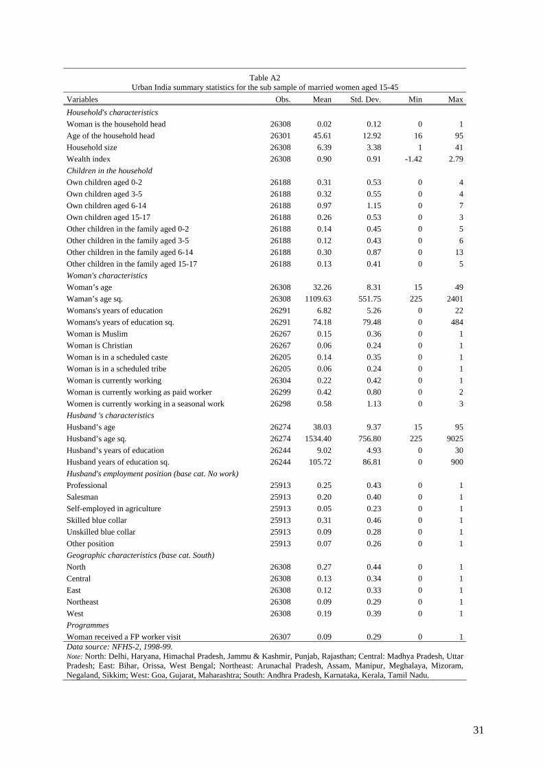
Table A2 Urban India summary statistics for the sub sample of married women aged 15-45

Variables Obs. Mean Std. Dev. Min MaxHousehold's characteristics Woman is the household head 26308 0.02 0.12 0 1Age of the household head 26301 45.61 12.92 16 95Household size 26308 6.39 3.38 1 41Wealth index 26308 0.90 0.91 -1.42 2.79Children in the household Own children aged 0-2 26188 0.31 0.53 0 4Own children aged 3-5 26188 0.32 0.55 0 4Own children aged 6-14 26188 0.97 1.15 0 7Own children aged 15-17 26188 0.26 0.53 0 3Other children in the family aged 0-2 26188 0.14 0.45 0 5Other children in the family aged 3-5 26188 0.12 0.43 0 6Other children in the family aged 6-14 26188 0.30 0.87 0 13Other children in the family aged 15-17 26188 0.13 0.41 0 5Woman's characteristics Woman’s age 26308 32.26 8.31 15 49Waman’s age sq. 26308 1109.63 551.75 225 2401Womans's years of education 26291 6.82 5.26 0 22Womans's years of education sq. 26291 74.18 79.48 0 484Woman is Muslim 26267 0.15 0.36 0 1Woman is Christian 26267 0.06 0.24 0 1Woman is in a scheduled caste 26205 0.14 0.35 0 1Woman is in a scheduled tribe 26205 0.06 0.24 0 1Woman is currently working 26304 0.22 0.42 0 1Woman is currently working as paid worker 26299 0.42 0.80 0 2Women is currently working in a seasonal work 26298 0.58 1.13 0 3Husband 's characteristics Husband’s age 26274 38.03 9.37 15 95Husband’s age sq. 26274 1534.40 756.80 225 9025Husband’s years of education 26244 9.02 4.93 0 30Husband years of education sq. 26244 105.72 86.81 0 900Husband's employment position (base cat. No work) Professional 25913 0.25 0.43 0 1Salesman 25913 0.20 0.40 0 1Self-employed in agriculture 25913 0.05 0.23 0 1Skilled blue collar 25913 0.31 0.46 0 1Unskilled blue collar 25913 0.09 0.28 0 1Other position 25913 0.07 0.26 0 1Geographic characteristics (base cat. South) North 26308 0.27 0.44 0 1Central 26308 0.13 0.34 0 1East 26308 0.12 0.33 0 1Northeast 26308 0.09 0.29 0 1West 26308 0.19 0.39 0 1Programmes Woman received a FP worker visit 26307 0.09 0.29 0 1Data source: NFHS-2, 1998-99. Note: North: Delhi, Haryana, Himachal Pradesh, Jammu & Kashmir, Punjab, Rajasthan; Central: Madhya Pradesh, Uttar Pradesh; East: Bihar, Orissa, West Bengal; Northeast: Arunachal Pradesh, Assam, Manipur, Meghalaya, Mizoram, Negaland, Sikkim; West: Goa, Gujarat, Maharashtra; South: Andhra Pradesh, Karnataka, Kerala, Tamil Nadu.

31

Table A3 Rural India summary statistics for the sub sample of married women aged 15-49

Variables Obs. Mean Std. Dev. Min MaxHousehold's characteristics Woman is the household head 58510 0.02 0.14 0 1Age of the household head 58499 45.49 13.80 2 95Household size 58510 7.02 3.72 1 46Wealth index 58510 -0.38 0.75 -1.53 2.71Children in the household Own children aged 0-2 58177 0.38 0.56 0 4Own children aged 3-5 58177 0.41 0.61 0 6Own children aged 6-14 58177 1.09 1.24 0 7Own children aged 15-17 58177 0.24 0.49 0 4Other children in the family aged 0-2 58177 0.21 0.54 0 6Other children in the family aged 3-5 58177 0.18 0.53 0 7Other children in the family aged 6-14 58177 0.43 1.03 0 16Other children in the family aged 15-17 58177 0.19 0.49 0 5Woman's characteristics Woman’s age 58510 30.48 8.72 15 49Waman’s age sq. 58510 1005.11 559.70 225 2401Womans's years of education 58490 2.71 3.90 0 22Womans's years of education sq. 58490 22.54 42.08 0 484Woman is Muslim 58346 0.11 0.31 0 1Woman is Christian 58346 0.05 0.22 0 1Woman is in a scheduled caste 58006 0.18 0.39 0 1Woman is in a scheduled tribe 58006 0.14 0.35 0 1Woman is currently working 58499 0.39 0.49 0 1Woman is currently working as paid worker 23784 0.56 0.50 0 1Women is currently working in a seasonal work 23775 1.43 0.58 1 3Husband 's characteristics Husband’s age 58237 36.49 9.97 15 97Husband’s age sq. 58237 1431.30 789.84 225 9409Husband’s years of education 58405 5.49 4.75 0 30Husband years of education sq. 58405 52.62 62.95 0 900Husband's employment position (base cat. No work) Professional 58024 0.08 0.28 0 1Salesman 58024 0.07 0.26 0 1Self-employed in agriculture 58024 0.50 0.50 0 1Skilled blue collar 58024 0.18 0.38 0 1Unskilled blue collar 58024 0.10 0.30 0 1Other position 58024 0.04 0.20 0 1Geographic characteristics (base cat. South) North 58510 0.22 0.41 0 1Central 58510 0.21 0.40 0 1East 58510 0.20 0.40 0 1Northeast 58510 0.13 0.34 0 1West 58510 0.08 0.27 0 1Prime age facilities Primary school in the village 58510 0.90 0.30 0 1Anganwadi in the village 58343 0.67 0.47 0 1Family Planning Woman received a FP worker visit (dummy) 58509 0.12 0.32 0 1FP worker visit in the village (dummy) 58510 0.67 0.47 0 1FP visit percentage of beneficiaries 58510 2.16 2.87 0 22.86GP- Welfare and Labour Market Programmes

32

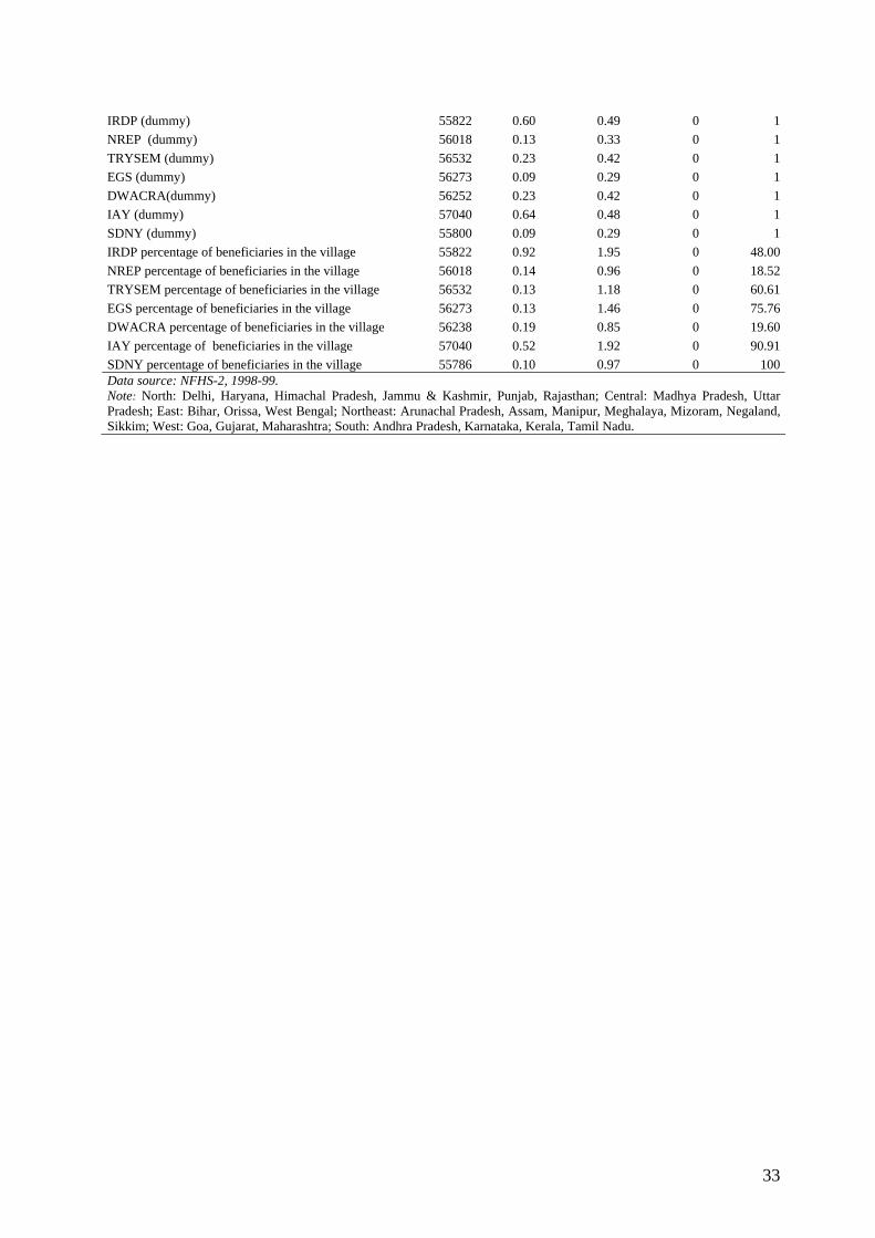
IRDP (dummy) 55822 0.60 0.49 0 1NREP (dummy) 56018 0.13 0.33 0 1TRYSEM (dummy) 56532 0.23 0.42 0 1EGS (dummy) 56273 0.09 0.29 0 1DWACRA(dummy) 56252 0.23 0.42 0 1IAY (dummy) 57040 0.64 0.48 0 1SDNY (dummy) 55800 0.09 0.29 0 1IRDP percentage of beneficiaries in the village 55822 0.92 1.95 0 48.00NREP percentage of beneficiaries in the village 56018 0.14 0.96 0 18.52TRYSEM percentage of beneficiaries in the village 56532 0.13 1.18 0 60.61EGS percentage of beneficiaries in the village 56273 0.13 1.46 0 75.76DWACRA percentage of beneficiaries in the village 56238 0.19 0.85 0 19.60IAY percentage of beneficiaries in the village 57040 0.52 1.92 0 90.91SDNY percentage of beneficiaries in the village 55786 0.10 0.97 0 100Data source: NFHS-2, 1998-99. Note: North: Delhi, Haryana, Himachal Pradesh, Jammu & Kashmir, Punjab, Rajasthan; Central: Madhya Pradesh, Uttar Pradesh; East: Bihar, Orissa, West Bengal; Northeast: Arunachal Pradesh, Assam, Manipur, Meghalaya, Mizoram, Negaland, Sikkim; West: Goa, Gujarat, Maharashtra; South: Andhra Pradesh, Karnataka, Kerala, Tamil Nadu.

33

Table A4

MARGINAL EFFECTS OF THE PROBABILITY OF WORKING OF MARRIED WOMEN AGED 15-49– MULTINOMIAL LOGIT - All India

marginal effects*100 - standard errors in italics

Household's characteristics Not

workingWorking

unpaidWorking

paid

Woman is the household head -7.69*** 4.45*** 3.24*** -0.01 0.01 0.01 Age of the household head 0.08*** -0.02*** -0.06*** 0.0002 -0.0001 -0.0001 Household size 0.76*** 0.53*** -1.29*** 0.001 0.001 -0.001 Wealth index 9.36*** -3.26*** -6.10*** 0.003 -0.002 -0.003 Children in the household Own children aged 0-2 6.14*** -1.82*** -4.32*** 0.004 -0.002 -0.003 Own children aged 3-5 -0.34 -0.21 0.55* -0.003 -0.002 0.003 Own children aged 6-14 -1.28*** -0.27*** 1.55*** -0.002 -0.001 0.002 Own children aged 15-17 -1.02*** -0.13 1.15*** -0.004 -0.002 0.003 Other children in the family aged 0-2 -0.10 -0.40* 0.501 -0.005 -0.002 0.005 Other children in the family aged 3-5 -0.10 -0.50** 0.61 -0.005 -0.002 0.005 Other children in the family aged 6-14 -0.52* -0.44*** 0.96*** -0.003 -0.001 0.003 Other children in the family aged 15-17 -0.58 0.02 0.56 -0.005 0.002 0.004 Woman's characteristics Woman’s age -2.01*** 0.38*** 1.62*** -0.002 0.001 0.002 Waman’s age sq. 0.02*** -0.004*** -0.02*** 0.00003 -0.00002 -0.00003 Womans's years of education 3.53*** -0.55*** -2.99*** 0.001 -0.001 -0.001 Womans's years of education sq. -0.29*** -0.06 0.30*** -0.0001 -0.0001 0.0001 Woman is Muslim 7.64*** -1.49*** -6.15*** 0.005 -0.003 -0.004 Woman is Christian -10.7*** 5.63*** 5.12*** 0.01 0.01 0.01 Woman is in a scheduled caste -4.54*** -3.10*** 7.64*** -0.005 -0.002 0.004 Woman is in a scheduled tribe -19.0*** 7.51*** 11.50*** -0.007 -0.004 0.006 Husband 's characteristics Husband’s age -0.26* 0.05 0.21 -0.002 0.001 0.001 Husband’s age sq. 0.004** -0.001 -0.003** 0.00002 -0.00001 -0.00002

34

Husband’s years of education 1.32*** 0.191*** -1.52*** 0.001 0.001 -0.001 Husband years of education sq. -0.03*** -0.008* 0.04*** -0.00008 -0.00005 0.00007 Husband's employment position (base cat. No work) Professional 1.75 1.93** -3.68*** 0.01 0.01 -0.01 Salesman 5.88*** 2.77*** -8.65*** 0.01 0.01 -0.01 Self-employed in agriculture -2.62** 6.91*** -4.29*** -0.01 0.01 -0.01 Skilled blue collar 5.08*** 0.06 -5.14*** 0.01 0.01 -0.01 Unskilled blue collar 7.83*** -3.30*** -4.53*** 0.009 -0.005 -0.008 Other position 5.97*** 1.04 -7.01*** 0.01 0.01 -0.01 Geographic characteristics (base cat. South) North 12.7*** 2.94*** -15.6*** 0.005 0.003 -0.003 Central 12.4*** -0.42 -12.00*** 0.005 -0.003 -0.003 East 21.8*** -7.72*** -14.0*** 0.004 -0.002 -0.003 Northeast 15.2*** -3.86*** -11.40*** 0.004 -0.003 -0.003 West -4.72*** 6.56*** -1.84*** -0.007 0.005 -0.005 Urban area 4.13*** -7.20*** 3.07*** 0.005 -0.002 0.004 Programmes Woman received a FP worker visit -3.26*** 0.55* 2.72***

-0.006 0.003 0.005

Observations 82225 Note: *** p<0.01, ** p<0.05, * p<0.1; +:dummy Data source: NFHS-2, 1998-99 Note: North: Delhi, Haryana, Himachal Pradesh, Jammu & Kashmir, Punjab, Rajasthan; Central: Madhya Pradesh, Uttar Pradesh; East: Bihar, Orissa, West Bengal; Northeast: Arunachal Pradesh, Assam, Manipur, Meghalaya, Mizoram, Negaland, Sikkim; West: Goa, Gujarat, Maharashtra; South: Andhra Pradesh, Karnataka, Kerala, Tamil Nadu.

35

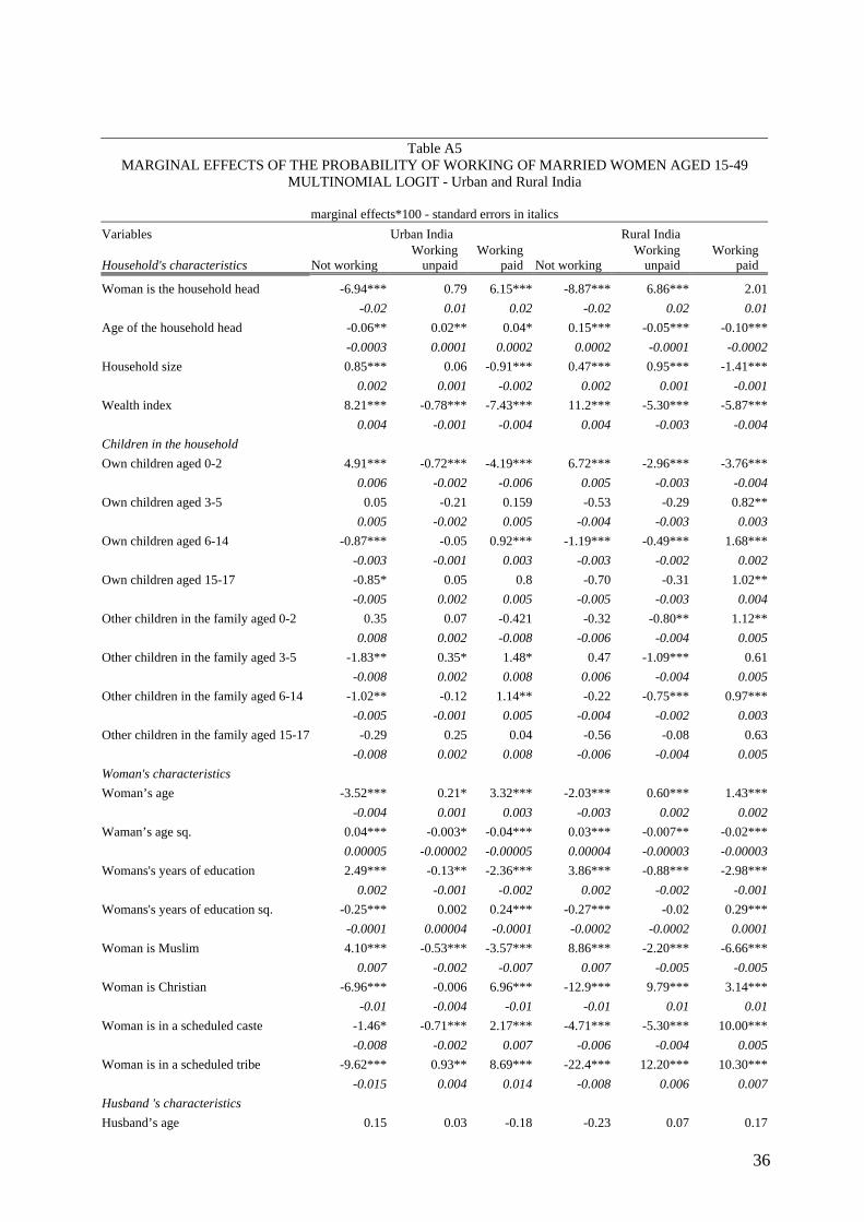
Table A5 MARGINAL EFFECTS OF THE PROBABILITY OF WORKING OF MARRIED WOMEN AGED 15-49

MULTINOMIAL LOGIT - Urban and Rural India

marginal effects*100 - standard errors in italics Variables Urban India Rural India

Household's characteristics Not working Working

unpaid Working

paid Not working Working

unpaid Working

paid

Woman is the household head -6.94*** 0.79 6.15*** -8.87*** 6.86*** 2.01 -0.02 0.01 0.02 -0.02 0.02 0.01Age of the household head -0.06** 0.02** 0.04* 0.15*** -0.05*** -0.10*** -0.0003 0.0001 0.0002 0.0002 -0.0001 -0.0002Household size 0.85*** 0.06 -0.91*** 0.47*** 0.95*** -1.41*** 0.002 0.001 -0.002 0.002 0.001 -0.001Wealth index 8.21*** -0.78*** -7.43*** 11.2*** -5.30*** -5.87*** 0.004 -0.001 -0.004 0.004 -0.003 -0.004Children in the household Own children aged 0-2 4.91*** -0.72*** -4.19*** 6.72*** -2.96*** -3.76*** 0.006 -0.002 -0.006 0.005 -0.003 -0.004Own children aged 3-5 0.05 -0.21 0.159 -0.53 -0.29 0.82** 0.005 -0.002 0.005 -0.004 -0.003 0.003Own children aged 6-14 -0.87*** -0.05 0.92*** -1.19*** -0.49*** 1.68*** -0.003 -0.001 0.003 -0.003 -0.002 0.002Own children aged 15-17 -0.85* 0.05 0.8 -0.70 -0.31 1.02** -0.005 0.002 0.005 -0.005 -0.003 0.004Other children in the family aged 0-2 0.35 0.07 -0.421 -0.32 -0.80** 1.12** 0.008 0.002 -0.008 -0.006 -0.004 0.005Other children in the family aged 3-5 -1.83** 0.35* 1.48* 0.47 -1.09*** 0.61 -0.008 0.002 0.008 0.006 -0.004 0.005Other children in the family aged 6-14 -1.02** -0.12 1.14** -0.22 -0.75*** 0.97*** -0.005 -0.001 0.005 -0.004 -0.002 0.003Other children in the family aged 15-17 -0.29 0.25 0.04 -0.56 -0.08 0.63 -0.008 0.002 0.008 -0.006 -0.004 0.005Woman's characteristics Woman’s age -3.52*** 0.21* 3.32*** -2.03*** 0.60*** 1.43*** -0.004 0.001 0.003 -0.003 0.002 0.002Waman’s age sq. 0.04*** -0.003* -0.04*** 0.03*** -0.007** -0.02*** 0.00005 -0.00002 -0.00005 0.00004 -0.00003 -0.00003Womans's years of education 2.49*** -0.13** -2.36*** 3.86*** -0.88*** -2.98*** 0.002 -0.001 -0.002 0.002 -0.002 -0.001Womans's years of education sq. -0.25*** 0.002 0.24*** -0.27*** -0.02 0.29*** -0.0001 0.00004 -0.0001 -0.0002 -0.0002 0.0001Woman is Muslim 4.10*** -0.53*** -3.57*** 8.86*** -2.20*** -6.66*** 0.007 -0.002 -0.007 0.007 -0.005 -0.005Woman is Christian -6.96*** -0.006 6.96*** -12.9*** 9.79*** 3.14*** -0.01 -0.004 -0.01 -0.01 0.01 0.01Woman is in a scheduled caste -1.46* -0.71*** 2.17*** -4.71*** -5.30*** 10.00*** -0.008 -0.002 0.007 -0.006 -0.004 0.005Woman is in a scheduled tribe -9.62*** 0.93** 8.69*** -22.4*** 12.20*** 10.30*** -0.015 0.004 0.014 -0.008 0.006 0.007Husband 's characteristics Husband’s age 0.15 0.03 -0.18 -0.23 0.07 0.17

36

0.003 0.001 -0.003 -0.002 0.001 -0.002Husband’s age sq. 0.001 -0.0007 -0.0004 0.004* -0.001 -0.002 0.00003 -0.00001 -0.00003 0.00002 -0.00002 -0.00002Husband’s years of education 0.86*** 0.02 -0.87*** 1.33*** 0.31*** -1.64*** 0.002 0.001 -0.002 0.001 0.001 -0.001Husband years of education sq. -0.009 -0.003 0.01 -0.042*** -0.01 0.05*** -0.00010 -0.00004 0.00010 0.00011 -0.00008 0.00009Husband's employment position (base cat. No work) Professional 3.64*** -0.17 -3.47*** -0.53 4.55*** -4.02*** 0.01 -0.01 -0.01 -0.02 0.02 -0.01Salesman 7.10*** 1.36* -8.46*** 5.20*** 3.16** -8.36*** 0.01 0.01 -0.01 -0.02 0.02 -0.01Self-employed in agriculture -2.88 6.98*** -4.10*** -4.74*** 9.84*** -5.10*** -0.02 0.02 -0.01 -0.01 0.01 -0.01Skilled blue collar 6.00*** -0.07 -5.93*** 3.59** 0.27 -3.85*** 0.01 0.005 -0.01 -0.02 0.01 -0.01Unskilled blue collar 4.01*** -0.33 -3.68*** 9.63*** -6.18*** -3.45*** 0.013 -0.005 -0.012 -0.013 -0.009 -0.010Other position 6.09*** -0.54 -5.55*** 4.35** 2.95* -7.30*** 0.01 0.00 -0.01 -0.02 0.02 -0.01Geographic characteristics (base cat. South) North 2.83*** 0.28 -3.11*** 16.80*** 3.71*** -20.50*** 0.007 0.003 -0.007 -0.007 0.006 -0.003Central 5.18*** -0.33 -4.85*** 16.30*** -1.50*** -14.80*** 0.008 -0.003 -0.007 -0.006 -0.005 -0.004East 10.20*** -1.52*** -8.66*** 29.90*** -14.20*** -15.70*** 0.006 -0.002 -0.006 -0.005 -0.003 -0.003Northeast 2.05** -0.15 -1.89** 21.80*** -7.89*** -13.90*** 0.009 -0.003 -0.009 -0.006 -0.004 -0.004West -0.38 0.89*** -0.52 -13.30*** 13.10*** 0.21 -0.008 0.003 -0.007 -0.010 0.009 -0.006Programmes Woman received a FP worker visit -1.31 0.56* 0.75 -2.42*** 0.53 1.89*** -0.009 0.003 0.009 -0.007 -0.005 0.005Observations 25528 56697 Note: *** p<0.01, ** p<0.05, * p<0.1; +:dummy Data source: NFHS-2, 1998-99 Note: North: Delhi, Haryana, Himachal Pradesh, Jammu & Kashmir, Punjab, Rajasthan; Central: Madhya Pradesh, Uttar Pradesh; East: Bihar, Orissa, West Bengal; Northeast: Arunachal Pradesh, Assam, Manipur, Meghalaya, Mizoram, Negaland, Sikkim; West: Goa, Gujarat, Maharashtra; South: Andhra Pradesh, Karnataka, Kerala, Tamil Nadu.

37

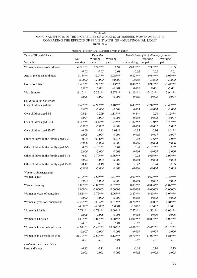
Table A6

MARGINAL EFFECTS OF THE PROBABILITY OF WORKING OF MARRIED WOMEN AGED 15-49 COMPARING THE EFFECTS OF FP VISIT WITH GP – MULTINOMIAL LOGIT

Rural India

marginal effects*100 - standard errors in italics Type of FP and GP var.: Dummies Beneficiaries (% of village population)

Variables Not working

Working unpaid

Working paid Not working

Working unpaid

Working paid

Woman is the household head -9.36*** 7.39*** 1.97 -9.83*** 7.98*** 1.85 -0.02 0.02 0.01 -0.02 0.02 0.01Age of the household head 0.13*** -0.04** -0.08*** 0.12*** -0.04*** -0.08*** 0.0002 -0.0002 -0.0002 0.0002 -0.0002 -0.0002Household size 0.48*** 0.95*** -1.43*** 0.48*** 0.96*** -1.44*** 0.002 0.001 -0.001 0.002 0.001 -0.001Wealth index 11.10*** -5.25*** -5.87*** 11.10*** -5.12*** -5.94*** 0.005 -0.003 -0.004 0.005 -0.003 -0.004Children in the household Own children aged 0-2 6.43*** -2.96*** -3.48*** 6.43*** -2.94*** -3.49*** 0.005 -0.004 -0.004 0.005 -0.004 -0.004Own children aged 3-5 -0.82* -0.299 1.11*** -0.84* -0.28 1.12*** -0.004 -0.003 0.004 -0.004 -0.003 0.004Own children aged 6-14 -1.35*** -0.42** 1.77*** -1.37*** -0.39** 1.76*** -0.003 -0.002 0.002 -0.003 -0.002 0.002Own children aged 15-17 -0.80 -0.21 1.01** -0.85 -0.16 1.01** -0.005 -0.004 0.004 -0.005 -0.004 0.004Other children in the family aged 0-2 -0.09 -0.88** 0.97* 0.02 -0.96** 0.94* -0.006 -0.004 0.006 0.006 -0.004 0.006Other children in the family aged 3-5 0.33 -1.01** 0.67 0.46 -1.13*** 0.67 0.006 -0.004 0.006 0.006 -0.004 0.006Other children in the family aged 6-14 -0.17 -0.70*** 0.86*** -0.22 -0.68*** 0.90*** -0.004 -0.003 0.003 -0.004 -0.003 0.003Other children in the family aged 15-17 -0.42 -0.19 0.62 -0.42 -0.24 0.65 -0.006 -0.004 0.005 -0.006 -0.004 0.005Woman's characteristics Woman’s age -2.10*** 0.63*** 1.47*** -2.07*** 0.59*** 1.48*** -0.003 0.002 0.002 -0.003 0.002 0.002Waman’s age sq. 0.03*** -0.007** -0.02*** 0.03*** -0.006** -0.02*** 0.00004 -0.00003 -0.00003 0.00004 -0.00003 -0.00003Womans's years of education 3.81*** -0.75*** -3.06*** 3.87*** -0.80*** -3.07*** 0.002 -0.002 -0.002 0.002 -0.002 -0.002Womans's years of education sq. -0.27*** -0.04** 0.31*** -0.28*** -0.03* 0.31*** -0.0002 -0.0002 0.0001 -0.0002 -0.0002 0.0001Woman is Muslim 7.72*** -1.72*** -6.00*** 7.57*** -1.50*** -6.08*** 0.008 -0.006 -0.006 0.008 -0.006 -0.006Woman is Christian -14.8*** 10.80*** 3.98*** -14.90*** 10.80*** 4.06*** -0.01 0.01 0.01 -0.01 0.01 0.01Woman is in a scheduled caste -4.91*** -5.40*** 10.30*** -4.69*** -5.45*** 10.10*** -0.007 -0.004 0.006 -0.007 -0.004 0.006Woman is in a scheduled tribe -21.70*** 12.60*** 9.13*** -20.70*** 11.90*** 8.81*** -0.01 0.01 0.01 -0.01 0.01 0.01Husband 's characteristics Husband’s age -0.22 0.11 0.1 -0.28 0.14 0.13 -0.002 0.002 0.002 -0.002 0.002 0.002

38

Husband’s age sq. 0.004* -0.002 -0.002 0.004* -0.002 -0.002 0.00002 -0.00002 -0.00002 0.00002 -0.00002 -0.00002Husband’s years of education 1.31*** 0.38*** -1.69*** 1.35*** 0.35*** -1.70*** 0.002 0.001 -0.001 0.002 0.001 -0.001Husband years of education sq. -0.04*** -0.02** 0.06*** -0.04*** -0.02* 0.06*** -0.0001 -0.0001 0.0001 -0.0001 -0.0001 0.0001Husband's employment position (base cat. No work) Professional -1.43 5.05*** -3.63*** -1.39 5.07*** -3.68*** -0.02 0.02 -0.01 -0.02 0.02 -0.01Salesman 4.78*** 3.18** -7.96*** 4.92*** 3.07* -7.99*** 0.02 0.02 -0.01 0.02 0.02 -0.01Self-employed in agriculture -5.62*** 10.50*** -4.90*** -5.50*** 10.50*** -4.97*** -0.02 0.01 -0.01 -0.02 0.01 -0.01Skilled blue collar 3.07* 0.41 -3.48*** 3.10** 0.33 -3.42*** 0.02 0.01 -0.01 0.02 0.01 -0.01Unskilled blue collar 9.65*** -6.29*** -3.35*** 9.47*** -6.27*** -3.20*** 0.01 -0.01 -0.01 0.01 -0.01 -0.01Other position 3.82** 3.48** -7.30*** 3.76** 3.55** -7.31*** 0.02 0.02 -0.01 0.02 0.02 -0.01Geographic characteristics (base cat. South) North 17.4*** 2.41*** -9.80*** 13.10*** 6.67*** -19.70*** 0.008 0.006 -0.004 0.008 0.007 -0.004Central 16.9*** -2.99*** -13.90*** 12.40*** 0.74 -13.10*** 0.007 -0.006 -0.004 0.008 0.006 -0.004East 30.00*** -15.20*** -14.80*** 27.50*** -13.10*** -14.40*** 0.005 -0.004 -0.004 0.006 -0.004 -0.004Northeast 22.30*** -9.53*** -12.80*** 19.40*** -6.87*** -12.50*** 0.006 -0.005 -0.004 -0.007 -0.006 -0.004West -9.69*** 10.90*** -1.23* -9.77*** 11.10*** -1.36** -0.01 0.01 -0.01 -0.01 0.01 -0.01Prime age facilities Primary school in the village -3.45*** -0.24 3.69*** -3.67*** -0.36 4.02*** -0.007 -0.006 0.005 -0.007 -0.006 0.005Anganwadi in the village -2.47*** 0.921** 1.55*** -2.18*** 0.4 1.78*** -0.005 0.004 -0.004 -0.005 0.004 -0.004Family Planning FP worker visit in the village (dummy) -5.26*** 0.38 4.88*** -0.005 0.004 0.004 FP visit percentage of beneficiaries -1.41*** 0.74*** 0.67*** -0.001 0.001 0.001GP- Welfare and Labour Market Programmes IRDP (dummy) 1.30** -1.82*** 0.52 0.005 -0.004 0.004 NREP (dummy) 4.37*** -3.09*** -1.27** 0.007 -0.005 -0.005 TRYSEM (dummy) 4.22*** -2.82*** -1.40*** 0.006 -0.004 -0.005 EGS (dummy) -3.32*** 2.26*** 1.05 -0.009 0.007 0.007 DWACRA(dummy) -0.133 -0.46 0.59 -0.006 -0.004 -0.005 IAY (dummy) -0.51 0.44 0.07 -0.005 -0.004 -0.004 SDNY (dummy) -4.04*** 1.58** 2.47*** -0.010 0.007 0.007

39

IRDP percentage of beneficiaries in the village 0.69*** -0.83*** 0.14 0.001 -0.001 0.001NREP percentage of beneficiaries in the village 0.58* -0.21 -0.37 0.003 -0.002 -0.003TRYSEM percentage of beneficiaries in the village 3.63*** -1.60*** -2.03*** 0.006 -0.004 -0.005EGS percentage of beneficiaries in the village -1.87*** 0.97*** 0.90*** -0.004 0.002 0.003DWACRA percentage of beneficiaries in the village -2.36*** 1.47*** 0.89*** -0.004 0.003 0.003IAY percentage of beneficiaries in the village -0.37 0.05 0.31* -0.002 0.002 0.002SDNY percentage of beneficiaries in the village -1.56*** 0.58** 0.98*** -0.005 0.002 0.003Observations 51746 51732

Note: *** p<0.01, ** p<0.05, * p<0.1; +:dummy Data source: NFHS-2, 1998-99 Note: North: Delhi, Haryana, Himachal Pradesh, Jammu & Kashmir, Punjab, Rajasthan; Central: Madhya Pradesh, Uttar Pradesh; East: Bihar, Orissa, West Bengal; Northeast: Arunachal Pradesh, Assam, Manipur, Meghalaya, Mizoram, Negaland, Sikkim; West: Goa, Gujarat, Maharashtra; South: Andhra Pradesh, Karnataka, Kerala, Tamil Nadu.

40