NBER WORKING PAPER SERIES

DO HOUSING PRICES REFLECT ENVIRONMENTAL HEALTH RISKS? EVIDENCEFROM MORE THAN 1600 TOXIC PLANT OPENINGS AND CLOSINGS

Janet CurrieLucas Davis

Michael GreenstoneReed Walker

Working Paper 18700http://www.nber.org/papers/w18700

NATIONAL BUREAU OF ECONOMIC RESEARCH1050 Massachusetts Avenue

Cambridge, MA 02138January 2013

Currie thanks the John D. and Catherine T. MacArthur Foundation and the Environmental ProtectionAgency (RE: 83479301-0) for support. Davis gratefully acknowledges research support from the NationalInstitutes of Health (R03ES016608). Walker acknowledges support from the Robert Wood JohnsonFoundation. We thank seminar participants at University of Delaware, MIT, Stanford, UC Davis, RAND,and the University of Oregon as well as Trudy Cameron for helpful comments. The research in thispaper was conducted while the authors were Special Sworn Status researchers of the U.S. Census Bureauwith generous guidance from Jim Davis, Jonathan Fisher, and Maggie Levenstein. Research resultsand conclusions expressed are those of the author and do not necessarily reflect the views of the CensusBureau, the MacArthur Foundation, the EPA, or the National Bureau of Economic Research. Thispaper has been screened to insure that no confidential data are revealed. A previous version of thispaper was circulated as “Toxic Pollutants and Infant Health: Evidence from Plant Openings and Closings”.

At least one co-author has disclosed a financial relationship of potential relevance for this research.Further information is available online at http://www.nber.org/papers/w18700.ack

NBER working papers are circulated for discussion and comment purposes. They have not been peer-reviewed or been subject to the review by the NBER Board of Directors that accompanies officialNBER publications.

© 2013 by Janet Currie, Lucas Davis, Michael Greenstone, and Reed Walker. All rights reserved.Short sections of text, not to exceed two paragraphs, may be quoted without explicit permission providedthat full credit, including © notice, is given to the source.

Do Housing Prices Reflect Environmental Health Risks? Evidence from More than 1600 ToxicPlant Openings and ClosingsJanet Currie, Lucas Davis, Michael Greenstone, and Reed WalkerNBER Working Paper No. 18700January 2013JEL No. D62,I18,Q51,Q53

ABSTRACT

A ubiquitous and largely unquestioned assumption in studies of housing markets is that there is perfectinformation about local amenities. This paper measures the housing market and health impacts of 1,600openings and closings of industrial plants that emit toxic pollutants. We find that housing values withinone mile decrease by 1.5 percent when plants open, and increase by 1.5 percent when plants close.This implies an aggregate loss in housing values per plant of about $1.5 million. While the housingvalue impacts are concentrated within 1/2 mile, we find statistically significant infant health impactsup to one mile away.

Janet CurriePrinceton University316 Wallace HallPrinceton, NJ 08544and NBERjcurrie@princeton.edu

Lucas DavisHaas School of BusinessUniversity of CaliforniaBerkeley, CA 94720-1900and NBERldavis@haas.berkeley.edu

Michael GreenstoneMIT Department of Economics50 Memorial Drive, E52-359Cambridge, MA 02142-1347and NBERmgreenst@mit.edu

Reed Walker50 University Hall, MC 7360Berkeley, CA 94720-7360rwalker@haas.berkeley.edu

!"!

1. Introduction

A ubiquitous and largely unquestioned assumption in studies of housing markets is that there

is perfect, or at least unbiased, information about local amenities and disamenities. This assumption

is critical because it has allowed for the generation of estimates of willingness to pay (WTP) for air

pollution, hazardous waste sites, health risks, school quality, local crime, climate, and many other

amenities and disamenties (e.g., Davis 2004 and 2011; Chay and Greenstone 2005; Greenstone and

Gallagher 2008; Linden and Rockoff 2008); these estimates are of interest in their own right but they

are also necessary for the development of optimal policy. However, there is virtually no direct

evidence on whether housing market participants are aware of the differences in amenities across

locations. The absence of this evidence undermines confidence in the reliability of the estimates of

WTP, especially in the case of environmental disamenities where there is often great scientific

uncertainty about the consequences of exposure.

Industrial plants that emit toxics are an especially important and salient local amenity. These

plants are ubiquitous in the United States today, and many lie in close proximity to major population

centers. Further, they emit nearly 4 billion pounds of toxic pollutants annually, including 80,000

different chemical compounds (GAO 2010).2 Whereas criteria air pollutants like sulfur dioxide have

been regulated for decades, regulation of other airborne toxics is in its infancy. The unveiling of the

Mercury and Air Toxics Standards in December 2011 represents the first time the U.S. government

has enforced limits on mercury and other toxic chemicals and most of the chemicals emitted have

never undergone any form of toxicity testing (U.S. Department of Health and Human Services

2010).3 Indeed, the existing evidence on toxic emissions is particularly sparse, despite the fact that

toxics are widely believed to cause cancer, birth defects, and damage to the brain and reproductive

systems (U.S. Centers for Disease Control and Prevention 2009). On the other side of the ledger,

these plants create jobs, increase local economic activity, and can lead to positive economic

spillovers (Greenstone, Hornbeck, and Moretti, 2010).

This paper represents a first step towards assessing the standard assumption of perfect or

unbiased information in the housing market. In doing so, we develop a research design to estimate

!!!!!!!!!!!!!!!!!!!!!!!!!!!!!!!!!!!!!!!!!!!!!!!!!!!!!!!!!!!!!2 Source: http://www.gao.gov/highrisk/risks/safety-security/epa_and_toxic_chemicals.php. Accessed on March 19th,

2012. 3 The Environmental Protection Agency characterizes their risk assessments as “not completely accurate” because “scientists don’t have enough information on actual exposure and on how toxic air pollutants harm human cells. The

exposure assessment often relies on computer models when the amount of pollutant getting from the source(s) to

people can’t be easily measured. Dose-response relationships often rely on assumptions about the effects of

pollutants on cells for converting results of animal experiments at high doses to human exposures at low doses.”

Source: http://www.epa.gov/ttn/atw/3_90_024.html (accessed on March 20, 2012).

!#!

the external costs of toxic plants in terms of both people’s willingness to pay to avoid toxic industrial

facilities and population health. We have assembled an extraordinarily rich dataset on the location

and economic activity of industrial plants in five large states in the United States. Our analysis

focuses, in particular, on plants that report toxic emissions to the U.S. Environmental Protection

Agency’s Toxic Release Inventory. We link information on these “toxic” plants with administrative

data that provides detailed information on the universe of housing transactions and birth outcomes in

these states. All three datasets provide exact geographic coordinates, so we are able to perform the

analysis with a high degree of spatial detail.

Our research design is based on the sharp change in local amenities that result from more

than 1,600 toxic plants opening and closing.4 The power of combining the 1,600 plus openings and

closings is that their staggered timing means that they form natural comparison groups for each other.

Further, the large number of changes in plant operations allows for an analysis based on millions of

births and hundreds of thousands of housing transactions. The remarkable spatial detail of our data

means that we can identify housing units and births both in the immediate vicinity of plants and

slightly farther away, allowing for comparisons both over time and across households living at

different distances from the plants.5

Since the previous literature offers little guidance about how far toxic pollutants travel, our

first contribution is to show that pollution emitted from toxic plants can be detected up to one mile

away from those plants. Using data from pollution monitoring stations and a difference-in-difference

estimator, we document significantly higher levels of ambient toxic pollution within one mile of

operating plants. On average, each birth in our sample lies within one mile of 1.27 toxic plants, so

our results imply that the total amount of exposure could be substantial. Moreover, these results

motivate our baseline research design, which compares households within one mile of a plant to

households one to two miles away.

We then turn to the housing market to assess the extent to which these 1600 plus plant

openings and closings are reflected in sales prices. If households have good information, then their

willingness-to-pay to avoid negative externalities should be reflected in housing price differentials.

Our preferred estimates imply that housing values are about 1.5 % lower within one mile of operating

!!!!!!!!!!!!!!!!!!!!!!!!!!!!!!!!!!!!!!!!!!!!!!!!!!!!!!!!!!!!!4 Indeed, our approach is inspired by a series of studies by C. Arden Pope and collaborators who examined the

health effects of opening and closing the Geneva steel mill near Provo, Utah in the late 1980s (Pope 1989; Ransom

and Pope 1992; Pope, Schwartz, and Ransom 1992). These studies have been influential largely because the resulting sharp changes in airborne particulates over a short period of time make the empirical analyses transparent

and highly credible. $There have been attempts to study the health and housing price responses of toxic emissions at the county level

(Agarwala, Banternghansa, and Bui 2010; Bui and Mayer 2003; Currie and Schmieder 2009), but counties are too

large due to the short transport distances of most airborne toxic pollutants (see Figure 1).

!%!

toxic plants. The results are roughly symmetric with housing prices decreasing when plants open and

increasing when plants close. We estimate that the aggregate loss in housing value per plant is

approximately $1.5 million. The effect is highly localized, with the largest impacts within a half-

mile radius of the plant.

Housing prices serve as a valuable summary measure of household welfare, but these

estimates will understate the economic cost of local externalities if there is imperfect information.

Many toxic pollutants are colorless, odorless, and not well monitored, making them less salient than

many other negative externalities. Thus, it is valuable to contrast housing prices with health

outcomes, which should immediately respond to changes in plant activity regardless of how well

these potential risks are understood. We find that the incidence of low birth weight increases by 2%

within one mile of operating toxic plants, with comparable magnitudes between 0 and 0.5 miles and

0.5 and 1 miles. Using an estimate of the monetary costs of low birth weight, this implies a total cost

per plant of $700,000 from this one health outcome alone. Again the effect appears to be roughly

symmetric in response to openings and closings, and again the effect appears to be highly localized,

with no impact beyond one mile.

Our study is one of the first large-scale empirical analyses of the external costs of toxic

plants. Whereas there are a handful of case studies of individual plants, relatively few studies have

examined multiple facilities, and our study is the first to bring together data from such a large

number of plants.6 This richness allows us to begin to characterize heterogeneity of effects across

plants. In additional results, we stratify plants by size and by the amount and toxicity of emissions,

finding that the housing price and health impacts are experienced broadly across different types of

plants. Interestingly, we find larger health impacts around plants that emit very toxic chemicals, but

limited evidence that this has a differential impact on housing values.

Our study is also the first in this literature to simultaneously examine both housing prices and

health outcomes. Some of the most suggestive results in the paper come from these comparisons. For

example, whereas the housing market impacts appear to be largely concentrated within a half mile,

the health effects are observed up to one mile away. This suggests that the health effects of toxic

plants may not disappear completely as soon as the plant closes, as would be the case if the causal

channel is water or ground pollution.

Lastly, we test whether household characteristics change when plants open and close.

!!!!!!!!!!!!!!!!!!!!!!!!!!!!!!!!!!!!!!!!!!!!!!!!!!!!!!!!!!!!!6 Studies of individual plants include the studies by C. Arden Pope mentioned above, as well as Blomquist (1974),

Nelson (1981), and Kiel and McClain (1995). For studies of multiple plants see, e.g., Bui and Mayer (2003) and

Davis (2011).

!&!

This analysis is of significant independent interest, as it provides new insight on the extent to which

populations migrate in response to changes in local amenities (Banzhaf and Walsh 2008). We find

that neighborhoods within one mile appear to have improved socio-economic status when plants are

in operation, suggesting that other things equal, infant health outcomes would improve rather than

deteriorate. Given previous evidence that educated, non-Hispanic white mothers are more likely to

move away from known hazards (Currie, 2011), this pattern suggests that the hazards posed by toxic

plants may not be widely recognized.

The rest of the paper proceeds as follows: Section 2 presents an analytical framework which

helps motivate the empirical analysis. Section 3 discusses the data, and Section 4 discusses the

research design. Sections 5 and 6 outline the econometric specifications and results for housing

values and infant health respectively. Finally, Section 7 interprets the results and 8 concludes.

2. Analytical Framework

2.1. The Incidence of Toxic Plant Openings

To motivate our empirical strategy, we outline a partial equilibrium model of housing

incidence in the context of toxic plant externalities.7 A local economy consists of a continuum of

agents of measure one (denoted !) that choose to live in one of two locations ! ! !!!!!; some

choose to live near a plant (! ! !) and others choose to live further away from a plant (! ! !), but

in the same local labor market. Toxic plant activity generates local economic benefits for both sets

of residents in the form of wage income, w. Wages are assumed to be an exogenous function of local

productivity and are the same across groups. Residents in each location enjoy location-specific

amenities net of any housing costs, Ag, associated with their location. Lastly, each resident ! has some

idiosyncratic preference for both locations, !!", representing heterogeneity in the valuation of local

amenities. The !!"’s are independently and identically distributed across individuals and assumed to

possess a continuous multivariate distribution with mean zero.

An individual seeks to maximize utility by choosing over locations

!!" ! !"# !! ! !!" ! !! ! !!" !

where !! represents mean utility in location g. Individuals will locate in whichever community yields

the highest utility. Without heterogeneity in locational preferences, all individuals will locate in the

community that offers the highest amenities. With heterogeneity in tastes, individuals in location N

!!!!!!!!!!!!!!!!!!!!!!!!!!!!!!!!!!!!!!!!!!!!!!!!!!!!!!!!!!!!!7 The results from this partial equilibrium exercise generalize into a model of general equilibrium of the sort found

in Kline (2010) and Moretti (2011). These models are themselves generalizations of the canonical models of Rosen

(1974) and Roback (1982).

!$!

will have!!! ! !! ! !!" ! !!". Define the distribution function !! ! !!" ! !!" by G(.). Then,

!! ! !"!!!! ! !! ! !!! is the measure of individuals in location N.

Write the total welfare of workers in location N and F as

! ! !!!"# !! ! !!" ! !! ! !!" !

And consider a positive economic shock stemming from a toxic plant opening in the community. We

model this shock as a marginal improvement in productivity in the local community, which is

assumed to increase wages in both the near and far locations equally. The plant opening, however,

creates a negative externality for residents living near the plant through, for example, air pollution

and related health effects.

Taking the derivative of workers welfare with respect to the economic shock associated with

a plant opening yields the expression:

(1) !"

!"! !! !

!"

!"! !! !

!"

!"!

!!!

!"! ! !

!"

!"! !! !

!!!

!"

where !" represents the marginal effect of a plant opening and !"

!!!

! !!.8 Equation (1) suggests the

incidence of the plant opening may be summarized by two terms. The first term is the total wage

effect associated with the plant opening. Since in our empirical application, all residents near or far

live within two miles of a plant, we assume that the wage effects are similar for both nearby residents

and those a little further from a plant. The second term consists of the non-wage changes in

amenities associated with a plant opening for residents near the plant. Since negative plant

externalities in the form of noise or air pollution are highly localized, these costs will only accrue to

the residents living near the plant.

After the plant opening some “marginal” residents who initially lived near the plant are better

off moving further away. However, since workers are optimizing with respect to location decisions, a

simple envelope result suggests that workers who switch locations in response to a change in local

amenities are to first order indifferent about doing so. Therefore, the incidence of the plant opening

may be approximated simply by the change in prices experienced by the immobile population. In the

case of non-marginal changes in productivity or local amenities, the envelope theorem no longer

holds, and taste-based sorting may also have first-order implications for welfare. However, in the

case of localized disamenities such as a single plant, Bartik (1987) and Palmquist (1992) show that

the slope of the hedonic price function is an approximate measure of the willingness to pay for a non-

!!!!!!!!!!!!!!!!!!!!!!!!!!!!!!!!!!!!!!!!!!!!!!!!!!!!!!!!!!!!!

8 The relationship !"

!!!! !! follows directly from assuming that preference heterogeneity is drawn from a Type I

Extreme Value distribution (Train 2003). However, this relationship also holds independent of the distribution of the

taste heterogeneity. See Busso, Gregory, and Kline (2011).

!'!

marginal change. See Greenstone and Gallagher (2008) for a more complete discussion of non-

marginal changes in the context of environmental amenities.9

This paper aims to estimate the local disamenities of toxic plant operation, !!!

!!, holding all

other factors fixed. We do this by comparing residents near a plant to those within the same local

labor market who live slightly further away. Since, by assumption, both groups are affected similarly

by the productivity shock, the difference-in-differences estimate will approximate !!!

!"! By explicitly

controlling for the first component of equation (1) in this way, our estimates will reflect the gross

external costs/benefits of a toxic plant opening or closing rather than the net external costs/benefits

after accounting for any local economic gains associated with toxic plant production.

2.2. Decomposing Housing Incidence: Pollution-Health Externalities

Housing prices serve as a useful way to track the costs and benefits of toxic plant activity,

and housing prices may offer the best data we have about people’s willingness to pay to avoid

disamenities.10 Nevertheless, housing values may not fully capture the amenities and disamenities

associated with toxic emissions if residents do not fully understand the risks. Many air pollutants are

colorless, odorless, and are not well monitored even though they may be harmful to human health.

Hence, to supplement our analysis of the housing market, we also explore implications for

the health of local communities surrounding toxic plants. We focus on infant health because it is one

of the few measures of population health that is available at a fine level of geographic disaggregation.

Infant health is also a key indicator of society’s well-being and an important determinant of an

individual’s future success in life (Currie, 2011). And focusing on infant health is advantageous,

relative to adult outcomes, because infants do not have a long unobserved health history. For

example, studies of the effects of pollution on adults are often plagued by concerns about previous

exposures and behaviors.

We believe this is the first large-scale study to present evidence on housing prices and health

outcomes in the same setting. Comparisons of the two sets of results provide some insight into the

operation of housing markets. For example, under the assumption that there are unbiased beliefs

about the infant health effects, it is possible to estimate the share of the observed effect on housing

prices accounted for by changes in infant health. Further, given our fine-grained spatial data, we can

assess whether the pattern of effects on housing prices matches the pattern of infant health effects.

This comparison can shed light on the validity of the assumption that the housing market has perfect

!!!!!!!!!!!!!!!!!!!!!!!!!!!!!!!!!!!!!!!!!!!!!!!!!!!!!!!!!!!!!9 Equilibrium sorting models may also yield insight into the welfare effects of non-marginal changes in the context

of environmental disamenities. See Kuminoff, Smith, and Timmins (2010) for a recent review. 10 The authors have often used these measures for this purpose. See, e.g., Currie and Walker (2011), Davis (2004,

2011), Chay and Greenstone (2005), and Greenstone and Gallagher (2008).

!(!

information about key amenities, which is an assumption that is central to the extensive hedonic

housing price literature.

3. Data Sources and Summary Statistics

3.1. The Toxic Release Inventory Data

We identify toxic plants using the Toxic Release Inventory (TRI), a publicly-available

database established and maintained by the U.S. Environmental Protection Agency (EPA).11 The TRI

was established by the Emergency Planning, Community Right to Know Act (EPCRA) in 1986, in

response to the Bhopal disaster and a series of smaller spills of dangerous chemicals at American

Union Carbide plants. Bhopal added urgency to the claim that communities had a “right to know”

about hazardous chemicals that were being used or produced in their midst. EPCRA requires

manufacturing plants (those in Standard Industrial Classifications 2000 to 3999) with more than 10

full-time employees that either use or produce more than threshold amounts of listed toxic substances

to report releases to the EPA.12

The toxic emissions measures in the TRI have been widely criticized (Marchi and Hamilton,

2006; Koehler and Spengler, 2007; Bennear, 2008). The emissions data are self-reported, and

believed to contain a large amount of measurement error.13 Moreover, coverage has expanded over

time to include additional industries and additional chemicals, making comparisons of total emissions

levels over time extremely misleading. 14 Finally, because of the minimum thresholds for reporting,

plants may go in and out of reporting even if they are continually emitting toxic chemicals. This

introduces additional measurement error, and also makes the TRI poorly suited for identifying plant

openings and closings.

The TRI is extremely useful, however, for identifying which U.S. industrial plants emit toxic

pollutants. The approach we adopt in this paper is to ignore, almost completely, the self-reported

magnitudes and instead exploit variation introduced by plant openings and closings. Using the

!!!!!!!!!!!!!!!!!!!!!!!!!!!!!!!!!!!!!!!!!!!!!!!!!!!!!!!!!!!!!11 See EPA (2007) and EPA (2011b) for detailed descriptions of the TRI. 12 Currently, facilities are required to report if they manufactured or processed more than 25,000 pounds of a listed

chemical or “otherwise used” 10,000 pounds of a listed chemical. For persistent bio-accumulative toxins, the

thresholds are lower. These thresholds have changed periodically over the life of the program. For example, in 1998,

EPA added the receipt or disposal of chemical waste to the definition of “otherwise used”. 13 The EPCRA explicitly states that plants need not engage in efforts to measure their emissions. The EPA provides

guidance about possible estimation methodologies, but plants estimate their emissions themselves, and estimating

methodologies vary between plants and over time. In addition, EPA enforcement of TRI reporting has typically taken the form of ensuring compliance rather than accuracy (Marchi and Hamilton, 2006). 14 Federal facilities were added in 1994. Mining, electric utilities, hazardous waste treatment and disposal facilities,

chemical wholesale distributors and other additional industrial sectors were added in 1998. Treatment of persistent

bio-accumulative toxins was changed in 2000. By the EPAs own admission, the TRI is not well suited for describing

changes in total amounts of toxic releases over time (U.S. EPA 2011b).

!)!

publicly-available TRI data, we create a list of all U.S. “toxic” plants by keeping every plant that

ever reported toxic emissions to the TRI in any year. This sidesteps the problems introduced by

changes in reporting requirements because plants end up being classified as “toxic” plants, even if,

for example, they are in industries which were not included in the early years of the TRI. We then

link this list of toxic plants to establishment-level data from the U.S. Census Bureau to determine the

exact years in which each plant opened (and closed, if applicable).

3.2. The Longitudinal Business Database

We determine the exact years in which plants open and close using the U.S. Census Bureau’s

Longitudinal Business Database (LBD). Started in 1975, the LBD is a longitudinal, establishment-

level database of the universe of establishments in the United States. 15 The LBD has been used

widely by economists, for example, in studying plant-level employment dynamics (Davis, Faberman,

Haltiwanger, Jarmin, and Miranda, 2010), and is by far the most accurate existing record of U.S.

plant activity. This precision is essential for our analysis, which relies largely on before and after

comparisons, exploiting the discrete changes in toxic emissions that occur at plant openings and

closings.

These data must be accessed at a census research data center under authorization from the

Census Bureau. They provide for each plant the year of opening (and closing, if applicable), as well

as mean annual employment and mean annual total salaries.16 We merge the LBD with a second

restricted access Census database called the Standard Statistical Establishment List (SSEL), which

contains plant names and addresses for all plants in the LBD. Finally, we merge the LBD/SSEL

dataset with the EPA’s TRI database via a name and address-matching algorithm.17

3.3. Housing Values

The housing data for this project includes housing transactions in five large states (Texas,

New Jersey, Pennsylvania, Michigan, and Florida). These data report the date, price, mortgage

amount, and address of all property sales for these five states from approximately 1998 to 2005.18

The data also include the exact street address of the property, which allows us to link the housing

data with plant level data from the TRI based on the latitude and longitude of the geocoded address

(described in more detail below). The main limitation of the housing data is that it contains very little

!!!!!!!!!!!!!!!!!!!!!!!!!!!!!!!!!!!!!!!!!!!!!!!!!!!!!!!!!!!!!15 For more information about the LBD see Davis, Haltiwanger, and Schuh (1998) and Jarmin and Miranda (2002). 16 The year of a plant opening is left-censored for those plants that were operating on or before 1975. 17 See Walker (2012) for further details pertaining to the match algorithm. 18 The transaction records are public due to state information disclosure acts, but the raw data are often housed in

PDF images on county websites making them inaccessible for computational analysis on a large scale. We used an

external data provider who compiled the information from the county registrar websites into a single dataset. Data

availability and temporal coverage varies by county but is fairly consistent between 1998-2005, the years of our

housing analysis.

!*!

information pertaining to housing unit characteristics.19 These data include both residential and

commercial real estate transactions, but we focus only on single-family, residential properties. To

limit the influence of outliers and focus on “arms length” transactions, we exclude properties that

sold for less than $25,000 or more than $10 million. All housing prices have been adjusted to year

2000 dollars.

3.4. Vital Statistics Data

Data on infant health comes from restricted-access vital statistics natality and mortality data

for the same five large states: Texas, New Jersey, Pennsylvania, Michigan, and Florida, from 1990 to

2002. Together, these states accounted for 10.9 million births between 1990-2002, approximately 37

percent of all U.S. births. The substantial advantage of these restricted-access data is their geographic

detail. Whereas publicly-available vital statistics data include only the county of residence, the

restricted-access data include the exact residential address of the mother. This precision is crucial in

our context because the health consequences of toxic plants are highly localized.

These data include detailed information about the universe of births and infant deaths in each

state. We focus, in particular, on whether the infant is low birth weight defined as birth weight less

than 2,500 grams. Low birth weight is common, affecting about seven percent of the births in our

sample. Low birth weight is one of the most widely used overall indicators of infant health, in part

because it has been shown to predict adult wellbeing.20 Other birth outcomes that we examine include

a continuous measure of birth weight, very low birth weight (defined as birth weight less than 1,500

grams), prematurity (defined as gestation less than 37 weeks), congenital abnormalities, and infant

mortality (death in the first year). These are all outcomes that have been previously examined in the

environment-infant health literature (e.g., Chay and Greenstone 2003; Currie, Neidell, and

Schmieder, 2009; Currie, Greenstone, and Moretti, 2011; and Currie and Walker, 2011). Because

there are many correlated outcomes and multiple hypothesis tests, we also construct a single,

standardized measure and perform a single hypothesis test (Hochberg, 1988; Kling, Liebman, and

Katz, 2007; Anderson 2008).

In addition to these health outcomes, the vital statistics data include a number of important

maternal characteristics including age, education, race, and smoking behavior. In the empirical

analyses below we control explicitly for these factors, as well as for month of birth, birth order, and

!!!!!!!!!!!!!!!!!!!!!!!!!!!!!!!!!!!!!!!!!!!!!!!!!!!!!!!!!!!!!19 For example, we observe square footage of the housing unit for less than half of the transactions. 20 Black, Devereux, and Salvanes (2007) use twin and sibling fixed effects models on data for all Norwegian births

over a long time period to show that birth weight has a significant effect on height and IQ at age 18, earnings, and

education. Using U.S. data from California, Currie and Moretti (2007) find that mothers who were low birth weight

have less education at the time they give birth and are more likely to live in a high poverty zip code. They are also

more likely to have low birth weight children.

!"+!

gender of child. In all analyses we exclude multiple births since they are likely to have poor birth

outcomes for reasons that have little to do with environmental pollution. We also test directly

whether plant openings and closings have affected these characteristics directly, either by changing

the composition of neighborhoods near plants and/or by changing fertility.

The fact that the LBD data is annual, while births are reported monthly raises the question of

how to best think about the timing of exposure. We retain births in November, December, January,

and February. Births in November and December are merged to LBD data from the same calendar

year, while births from January and February are merged to LBD data from the preceding calendar

year. The idea is that a baby born January 1, 2002 has not been exposed to any of the toxic plant

activity for calendar 2002, but was exposed to toxic emissions in 9 out of 12 months of 2001.

Similarly, a baby born in November 2001 was exposed to toxic emissions for 9 out of 12 months of

2001. This restriction has the additional advantage of limiting the extent to which seasonality in

plant activity or birth outcomes affects our findings.

3.5. Data Linkages and Aggregation

We link plants in the TRI and LBD to our vital statistics and housing data based on latitude

and longitude. Specifically, we first create a large dataset consisting of all pairwise combinations of

plants and outcome variables (i.e. births and/or housing transactions). We keep outcome variables

within two miles of a plant. This means that any outcome variable within two miles of more than one

plant will contribute one observation for each plant-outcome pair. We then collapse the outcome

measures into various distance bins surrounding plants in a given year. That is, for each plant-year,

we construct the mean of the outcome variable for outcomes that occurred within one mile of a plant

and the mean of the outcome variable for births that occurred between one and two miles of a plant.

We also use more granular distance bin definitions. Collapsing the data eases the computational

burden while also accounting for issues pertaining to inference when the identifying variation occurs

at a more aggregate level.

3.6. Summary Statistics

Panel A of Table 1 presents summary statistics for the sample of plants that form the basis for

our analysis. The three columns reflect the sample characteristics for plants that were always open,

newly opened, and newly closed within our sample frame respectively. Note that a single plant can

appear both in columns (2) and (3), although in practice the plants in our sample tend to be long-

lived, with a median age of around 17 years.21 For continuously operating plants, the mean value of

!!!!!!!!!!!!!!!!!!!!!!!!!!!!!!!!!!!!!!!!!!!!!!!!!!!!!!!!!!!!!21 Plant age in the LBD is left-censored in 1975 (the first year the plants are observed in the sample). Therefore, the

median age of the plants in our sample is likely to be a bit larger.

!""!

plant equipment and structures is $22 million, and mean annual salary and wages is $11.7 million.22

Mean salary and wages is lower for plants that opened or closed. The table also reports mean annual

toxic emissions, which exceeds 17,000 pounds in all three columns. These are the self-reported

measures of airborne toxic emissions from the TRI, and are averaged over all non-missing

observations (i.e. if a plant does not report to the TRI during a particular year in which we know the

plant is operating, we treat this as missing rather than zero).

Panel B of Table 1 describes community characteristics near plants that either opened or

closed during our sample period. Statistics are reported separately by distance to the plant and

observations are restricted to the 2 years after a plant opening or the 2 years before a plant closing.

Note that a house or birth can be close to more than one plant, and so the same house or birth can

appear in more than one column. Within columns, we have restricted houses and births so that they

appear only once in this panel, implicitly giving equal weight to each birth and housing outcome.

Both housing values and maternal characteristics tend to improve with distance from the

plant. The average housing value is $124,424 within a half mile of a plant compared to $132,227 for

houses between one and two miles away. Similarly, average maternal education rises from 11.93 to

12.22 over the same distance. In subsequent sections we examine how trends in these observables

evolve as a function of plant openings and closings, providing some additional insight into

population responses to changes in local disamenities. In addition, these sorting responses will help

us to interpret any measured health responses. Our identification strategy depends on the assumption

that there are smoothly evolving trends in both observable and unobservable characteristics of the

populations located less than a mile from a plant, and one to two miles from a plant.

These summary statistics describe how housing values and maternal characteristics vary with

distance, but don’t give a sense of how many toxic plants there are within different distances of a

given birth. Restructuring our dataset so that the unit of observation is a birth, we calculate that, on

average, there are 0.28 plants within a half mile of a birth, and 1.27 plants within one mile. In other

words, the average mother in our sample lives within one mile of 1.27 plants that emit toxic releases.

Restricting the sample to only sites where plants opened or closed between 1990 and 2002, there are

on average 0.10 sites within a half mile of a birth, and 0.32 sites within one mile.

!!!!!!!!!!!!!!!!!!!!!!!!!!!!!!!!!!!!!!!!!!!!!!!!!!!!!!!!!!!!!22 The capital stock measures come from the Annual Survey of Manufacturers, and are computed using a modified

perpetual inventory method (Mohr and Gilbert, 1996). Since the ASM is a sample and oversamples large

establishments, these statistics are not available for all plant years and reflect statistics for larger plants.

!"#!

4. The Transport of Airborne Toxics as the Basis of a Research Design

Our difference-in-differences strategy compares houses and births in areas “near” a toxic

plant to those in areas slightly farther away. While this is a simple idea conceptually, there is little

guidance in the literature about how near a household must be to a plant for proximity to affect either

housing prices or birth outcomes. In particular, atmospheric science provides little definitive

information about how far toxic emissions are transported so we instead characterize this relationship

empirically. This evidence is of significant independent interest and an important contribution of our

paper.

Our approach uses data from monitoring stations about ambient levels of hazardous air

pollution. While the EPA has been monitoring criteria air pollutants for four decades, they have only

recently begun monitoring hazardous air pollutants (HAPs).23 The first year of data availability was

1998 and monitors have been gradually added over time. As of 2003, the last year of our sample,

there were 84 pollutants being monitored across the 5 states in our sample. We standardize each

pollutant to have mean zero and standard deviation of one.24

We matched the monitoring station data to our data on toxic plants using latitude and

longitude, keeping monitor-plant pairs in which the plant had ever reported releasing the monitored

pollutant. We then examine the relationship between this standardized pollutant score and distance

from operating toxic plants using the following linear regression model,

(2) !"##!"# ! !! ! !!! !"#$%!!"#$%&'() !" !

!! !"#$%!!"#$%&'() !" ! !"#$%&'(!"!!!! ! !!" ! !! ! !!!"#

where the dependent variable is the standardized pollution measure for monitor m linked to plant j in

year t. The regression includes an indicator variable for whether a plant is operating in a given year,

and the interaction between the indicator and a polynomial in the distance between the plant and the

monitor. We also include monitor-plant pair fixed effects, !!", so that identification comes from

plant openings and closings. Lastly, we include year fixed effects, !!! to control for overall trends in

ambient pollution concentrations. The standard errors are two-way clustered on both monitor and

plant.

!!!!!!!!!!!!!!!!!!!!!!!!!!!!!!!!!!!!!!!!!!!!!!!!!!!!!!!!!!!!!23 Hazardous air pollutants, also known as toxic air pollutants, are defined by the EPA as “pollutants that are known

or suspected to cause cancer or other serious health effects, such as reproductive effects or birth defects, or adverse environmental effects.” In contrast, criteria air pollutants, are more commonly found air pollutants that are regulated

according to the EPA’s National Ambient Air Quality Standards (NAAQS). 24 Note that some pollutants are certainly more toxic or hazardous than others. For the purposes of this particular

econometric exercise, we are simply trying to understand if any detectible relationship exists between toxic plant

activity and ambient levels of hazardous air pollutants, irrespective of the toxicity of a given pollutant.

!"%!

Figure 1 plots the marginal effect of an operating plant on hazardous air pollution as a

function of distance from the plant to a monitor. Average levels of ambient hazardous air pollution

are one standard deviation higher immediately adjacent to an operating plant, and decline

exponentially with distance, reaching zero at roughly one mile from a plant. This figure was

constructed using a quartic in distance. We have also examined different functional forms for

distance and the results are similar.25

Documenting this relationship between toxic plant activity and ambient levels of hazardous

air pollution is valuable in its own right, but it also helps motivate our empirical specifications. There

are several ways for a plant to affect housing values and human health including aesthetics,

congestion, and noise. Toxic emissions may be among the channels that have the most distant effects,

and the evidence suggests that on average emissions do not reach further than one mile.26 This

finding underscores the importance of performing the analyses which follow using spatial data at a

high level of resolution. In most analyses below, we define “near” as within one mile of a plant and

“far” as one to two miles away. Due to their geographic proximity, houses and households within one

to two miles of the toxic plants are used as a comparison group for outcomes in the zero to one mile

range. We also present results using alternative distances. As discussed above, the underlying

assumption is that these individuals are close enough that they share in the wage and productivity

effects of the plant. Hence, differences in the impact of plant operations reflect the effects of the local

disamenities of plant operation.

5. Housing Values

5.1. Housing Values: Empirical Strategy

In order to investigate the effects of toxic plants on housing values we fit the following

econometric model:

(3) !!"# ! !!! ! !!! !"#$%!!"#$%&'() !" ! !!! ! !!!"#$ !" !!

!!! !"#$%!!"#$%&'() !" ! ! ! !!!"#$ !" ! !!!" ! !! ! !!!!!""#!" ! !! ! !!!"#

where !!"# denotes average housing values near plant site !, within distance group !, in year !. For

each plant j, there are two observations per year. In each plant-year, one observation consists of

average housing prices "near" a plant (i.e. within 1 mile of the plant), which is the distance that toxic

!!!!!!!!!!!!!!!!!!!!!!!!!!!!!!!!!!!!!!!!!!!!!!!!!!!!!!!!!!!!!25 Models using more flexible distance specifications, such as replacing a continuous distance measure with dummy

variables for different distance bins yield similar results, but the models are less precisely estimated. 26 A recent literature also finds that other forms of housing externalities are very localized (See for example, Linden

and Rockoff (2008), Harding, Rosenblatt, and Yao (2009), Rossi-Hansberg, Sarte, and Owens (2010), and

Campbell, Giglio, and Pathak (forthcoming)).

!"&!

air emissions travel. The second observation per plant-year consists of average house prices for

houses within 1-2 miles of the plant; this second group provides a counterfactual for housing prices

near the plant. The availability of these two groups allows for a difference in differences-style

estimator.

The variable ! !"#$%!!"#$%&'() !" is an indicator equal to one if a toxic plant ! is operating

in year ! and zero otherwise. It is equal to 1 for both distance groups associated with a plant. In

equation (3), we define "near" as being within one mile of and the indicator ! ! !!!"#$ !" is equal

to one if the house is within one mile of a location in which a toxic plant operated at any point in our

sample. Equation (3) also includes plant by distance fixed effects !!" to control for all time-invariant

determinants of house prices in a plant by distance group, which in practice is collinear with the

indicator ! ! !!!"#$ !". Additional controls include 1990 census tract characteristics !!""#!",

interacted with quadratic time-trends !!.27 Equation (3) also includes time fixed effects, !!, in order to

flexibly account for trends in housing values over time. In practice, we report specifications that

include either state by year fixed effects to account for regional patterns in housing prices or plant by

year fixed effects to account for very local trends in prices. The former specification requires the

estimation of 25 fixed effects, while the latter adds approximately 10,000 fixed effects, one for each

plant-year.

The parameter of interest in Equation (3) is !!, the coefficient on the interaction term,

! !"#$%!!"#$%&'() !" ! !!! !!!"#$!!". It captures the differential impact of an open plant on

locations within one mile, relative to those one to two miles away. Given that our models include

plant by distance fixed effects !!", !! is identified by changes in the operating status of a plant (i.e.

plant openings and closings). In the model that includes plant by year fixed effects (in addition to

plant by distance fixed effects), the identification of !! is based on within year comparisons of

changes in house prices among houses 0-1 and 1-2 miles from the location of toxic plant openings

and closings.

Finally, we estimate an alternative model that allows us to test whether the effects of plant

openings differ from those of plant closings. In this alternative model, the variable

! !"#$%!!"#$%&'() !" is replaced by two separate indicators ! !"#$%!!"#$#% !" and

! !"#$%!!"#$%& !". The variable ! !"#$%!!"#$#% !" is an indicator equal to zero before the plant

opens, and equal to one in all years after the plant opens, even if the plant subsequently closed. The

!!!!!!!!!!!!!!!!!!!!!!!!!!!!!!!!!!!!!!!!!!!!!!!!!!!!!!!!!!!!!27 Census tract characteristics were mapped to plant radii using ArcGIS, where the radius characteristics consist of

the area weighted averages of census tracts that intersect the distance circle/radius. Results are similar with and

without these controls.

!"$!

variable ! !"#$%!!"#$%& !" is an indicator variable equal to zero before the plant opens and while it

is operating, and then equal to one for all years after the plant closes. The parameters associated with

the interactions of these indicators with !!! !!!"#$!!" allows for a comparison of the differential

impacts of plant closings and openings on property values.

Finally, two other estimation details are worth noting. Equation (3) is estimated using

weighted least squares, with the weights equal to the number of homes in the respective plant by

distance group by year cell. The subsequent analysis reports conservative standard errors that are

two-way clustered by plant and year to allow for serial correlation within a plant over time as well as

for arbitrary forms of spatial correlation in a given year.

5.2. Housing Values: Results

Before turning to the parametric models, we present event study graphs that plot the effects

of plant openings and closings on housing values. These graphs are derived from the estimation of

versions of equation (3) that include plant by year fixed effects and allow the coefficients on

! !"#$%!!"#$#% !" ! !!! !!!"#$!!" and ! !"#$%!!"#$%& !" ! !!! !!!"#$!!" to vary with event

time, where year zero is the year that the plant's operating status changes (i.e., the year of the plant

opening or closing). The figures plot these coefficients and their 95% confidence intervals.28 The

figures preview the regression results that boil down to a comparison of the averages of the data

points to the left and right of the vertical lines. Further, they provide an opportunity to judge the

validity of the difference in a differences-style approach that is based on the assumption of similar

trends in advance of the opening or closing.29

The left panel of Figure 2 plots event study coefficients for years before/after a plant opening,

and the right panel plots event time coefficients before/after a plant closing. The plotted coefficients

represent the time path of housing values near to a plant (relative to far) conditional on

plant*distance and plant*year fixed effects. Both panels support the validity of the design as there is

little evidence of differential trends in housing prices between houses 0-1 and 1-2 miles from the

!!!!!!!!!!!!!!!!!!!!!!!!!!!!!!!!!!!!!!!!!!!!!!!!!!!!!!!!!!!!!28 The available housing price data only allow for the estimation of the coefficients for event years -3 through +5 for

plant openings and -5 through +5 for plant closings since plant openings are concentrated in the earlier part of our

sample. 29 We estimate the event-study graphs separately for plant openings and plant closings. In particular, we fit the

following regression model, reporting the event-time coefficients, !!:

!!"# ! !!! ! !!! !!" !! ! ! ! ! !!!"#$ !"

!

!!!!

! ! !" ! !" ! !!!!!""#!"

where ! !!" !! ! is an event-time indicator equal to 1 for each of the years prior and after a plant opening or

closing. In the presence of plant*distance fixed effects !!" not all the event-time indicators are identified. For this

reason, we normalize the coefficient on the indicator for ! !!" !! !! to be equal to zero.

!"'!

plant. Further, they both suggest that the changes in plant operating status affected housing prices. In

the left panel, housing prices are lower after the plant opening and in the right panel they are higher

after a plant closing. Notably in both panels, there appears to be a jump in housing prices in the year

where the plant's operating status changed. It is also apparent that the estimates for plant openings are

noisier which is to be expected because there are relatively fewer plant openings than closings during

the period covered by the housing price data (i.e., 70 openings and 544 closings).

Table 2 reports the baseline estimates for the effects of toxic plant operation on housing

values from 16 separate regressions. Panel (A) reports the coefficient and standard error associated

with the interaction of ! !"#$%!!"#$%&'() !" ! !! ! !!!"#$ !", while Panel (B) allows the effects of

openings and closings to differ; it also reports the p-value from a test that the opening coefficient is

equal to the negative of the closing coefficient. In all regressions the comparison group is homes

located between one and two miles, whereas the definition of “near” changes across regressions, as

indicated by the column headings. The odd numbered columns report on specifications that include

state by year fixed effects and the even numbered ones are from specifications that alternatively use

plant by year fixed effects. We estimate these models on a balanced panel of plant*distance*year

observations, excluding a subset of plants for which no housing values occurred in a specific

distance*year.30

The estimates suggest that toxic plant operations reduce housing values in the immediate

vicinity of the plant. Columns (1) and (2) indicate that an operating toxic plant within a half mile is

associated with a 2 to 3% percent decrease in housing values. Within a half mile of a plant, the

effects of openings and closings are opposite in sign, although the effect of plant openings is not well

identified. The estimates suggest that housing values decrease by 1 to 2% within a half mile when a

plant opens, and then increase by 2 to 3% when a plant closes. However, we cannot reject the null

that the opening coefficient is equal to -1 times the closing coefficient.

The point estimates in columns (3) and (4) are generally of a smaller magnitude, suggesting

that the effects of plant operations on housing values to fade with distance. For example, the point

estimate in column 3 suggests that the effect of plant operations on housing values falls to one

percent in the half mile to one mile range. The standard errors are large enough, however, that their

95 % confidence intervals overlap the 95% confidence intervals of the estimates in columns (1) and

(2). Hence, in columns (5) and (6) we compare the entire zero to one mile area with the one to two

!!!!!!!!!!!!!!!!!!!!!!!!!!!!!!!!!!!!!!!!!!!!!!!!!!!!!!!!!!!!!30 Results using an unbalanced panel are similar. Models estimated using plant*year fixed effects are estimated in

two steps. The first step demeans all regression model variables by plant*year. The second step then estimates the

model on the remaining covariates using the demeaned data.

!"(!

mile zone.31 Not surprisingly given the previous estimates, the overall impact on housing values

within one mile is about -1.5%. Additionally, we cannot reject the null that openings and closings are

equal but of opposite sign, though only the effects of closings are statistically significant in these

models.

The last two columns of Table 2 drop observations that identify coefficients on event years

prior to -2 and after 2. Focusing on the years immediately before and after a plant opening or closing

also helps to measure shifts in the demand for housing along an inelastic short-run housing supply

curve, since longer run estimates will reflect shifts in both supply and demand. This restriction

attenuates the point estimates, but we cannot reject the null hypothesis that these results are the same

as our baseline results in columns (5) and (6).

Results are similar when we use a comparison group of two to four miles from a plant instead

of one to two miles. See Appendix Table A1. This is reassuring because it suggests that the results

are not driven by patterns in housing prices in the one to two mile zone. Nonetheless, it is possible

that plant disamenities could lead to a reduction in housing demand in nearby (i.e., 0-1 miles)

locations and a corresponding increase in housing demand in locations farther away. This type of

preference-based sorting, which we investigate in more detail in subsequent sections, would lead us

to over-estimate the housing price response of the plant in the 0-1 mile range. We investigate this

issue further by estimating alternative models for home prices within mutually exclusive concentric

rings around the plant.

Appendix Table A.2 presents regressions based on the following econometric model,

restricting the sample to different distance bandwidths (e.g. 0 to 0.5 miles, 0.5 to 1 miles, 1 to 1.5

miles, 1.5 to 2.0 miles, etc…):

(4) !!" ! !!! ! !!! !"#$%!!"#$%&'() !" ! !!! ! !! ! !!!!!""#!" ! !! ! !!!".

The coefficient of interest is !!, which captures the relationship between plant operating activity and

housing values. The specification includes a plant level fixed effect (!!!!so that !! is identified by

pre-post comparisons of housing prices in areas with plant openings or closings.32 We report on a

specification that includes year fixed effects and a second one that replaces them with state by year

fixed effects. In these models, the comparison group is no longer houses within the same community,

but further away from the plant: instead, the comparison group consists of houses within the same

distance from a toxic plant in other communities that did not experience an opening or closing.

!!!!!!!!!!!!!!!!!!!!!!!!!!!!!!!!!!!!!!!!!!!!!!!!!!!!!!!!!!!!!31 The column (6) specification is the difference-in-differences analogue to the event-time regression plotted in

Figure 2. 32 Note, there is only one distance category in each regression so that a plant*distance fixed effect would be

redundant in this class of models.

!")!

The estimates in Appendix Table A.2 corroborate our baseline findings and choice of

comparison group; the effects of plant operating status are highly localized, and there seems to be

little negative effect of plant openings in areas more than one mile away from a plant. These

estimates suggest that an operating plant reduces housing values by about 2 percent within a half

mile of a plant and closer to 1 percent in the 0.5 to 1 mile range although this is estimated less

precisely. However, there is little evidence of an effect on housing prices at further distances.

Thus far we have concentrated on the average effect of a plant opening or plant closing.

However, this focus obscures a tremendous amount of heterogeneity across plants. Table 3 explores

heterogeneity in our baseline estimates by stratifying plants across different observable

characteristics. We group plants into whether their median value of a particular variable of interest

(taken over years of plant operation) is above or below the population median (taken over the plant-

level medians). The characteristics we explore are plant employment, payroll, stack emissions,

fugitive emissions, mean toxicity of chemicals released, and the maximum toxicity of the chemicals

released. These toxicity measures were calculated using the EPA’s Risk-Screening Environmental

Indicators.33 Plants report in the TRI both stack and fugitive emissions. Stack emissions occur during

the normal course of plant operations, emitted via a smoke stack or some other form of venting

equipment which is, in many cases, fitted with pollution abatement equipment. Because stacks are

often extremely high, these emissions may tend to be dispersed over a wide geographic area. Fugitive

emissions are those that escape from a plant unexpectedly, generally without being treated. These

emissions may be more likely to be manifest to households in the form of noxious odors or residues.

Table 3 shows that the effect of plants on housing values is greater for larger plants (as

measured by employment and payroll). In addition, there is evidence that plants emitting large

amounts of fugitive emissions have a more negative effect on housing values than those emitting

fewer fugitive emissions. Conversely, for stack releases, the point estimates for plants below the

median is larger. However, since the 95% confidence intervals of each of the pairs of estimates

overlap, the estimates are not precise enough for definitive conclusions.

Turning to the toxicity of releases, the estimates suggest that housing prices respond more to

high mean toxicity than to high maximum. If households were aware of these toxicity measures and

they were valued (negatively) by households, one would have expected to see this reflected in

housing price differentials and the lack of a robust pattern between plants with high and low toxicity

is consistent with households having imperfect information. In addition to the imprecision of these

!!!!!!!!!!!!!!!!!!!!!!!!!!!!!!!!!!!!!!!!!!!!!!!!!!!!!!!!!!!!!33 Surprisingly little is known about the relative toxicity of different chemicals. Although animal testing is broadly

used for evaluating the toxicity of chemical compounds, these studies are of limited relevance for evaluating which

chemicals are likely to be most damaging for human health.

!"*!

estimates, it is also noteworthy that there is little scientific evidence on how the health effects of

exposure vary with these measures of toxicity.

6. Infant Health

6.1. Infant Health: Empirical Strategy

The empirical strategy for examining infant health outcomes is very similar to the approach

used for housing values. Again, our main focus is on comparing outcomes within one mile of a plant

to outcomes between one and two miles,

(5) !!"# ! !!! ! !!! !"#$%!!"#$%&'() !" ! !!! ! !!!"#$ !" !

!!! !"#$%!!"#$%&'() !" ! !! ! !!!"#$ !" ! !!!" ! !! ! !!!!!""#!" ! !!! ! !!"#

where !!"# denotes the average incidence of low birthweight or another measure of infant health near

plant site !, within distance group !, in year !.

This estimating equation is almost identical to the estimating equation used for housing

values. Again, the coefficient of interest, now denoted !!, is the differential impact of an operating

plant within one mile. As before, the specification includes plant by distance fixed effects !!", year

fixed effects !! (which in practice are state by year or plant by year fixed effects), and census controls

!!""#!" interacted with quadratic time-trends !!. We again explore possible asymmetries in the

health impacts of plant openings and closings.

The vital statistics data include a rich set of mother’s characteristics that can be used to

control for possible changes in the composition of mothers (explored further below). However, the

identifying variation in our models comes at a much higher level of aggregation; hence, in order to

avoid overstating the precision of our estimates we control for mother's characteristics using a two-

step, group-level estimator (Baker and Fortin, 2001; Donald and Lang, 2007). In the first step, we

estimate the relationship between low birth weight (!!"#! and plant by distance by year indicators

(!!"#!, after controlling for mother’s characteristics (!!"):

(6) !!"# ! !!!!"! ! !!"# ! !!"#!

The vector !!" controls for maternal characteristics including indicators for: age categories (19-24,

25-34, and 35+), education categories (<12, high school, some college, and college or more), race

(African American or Hispanic), smoking during pregnancy, month of birth, birth order, and gender

of child.34 The estimated !!"# provide group-level, residualized averages of each specific birth

!!!!!!!!!!!!!!!!!!!!!!!!!!!!!!!!!!!!!!!!!!!!!!!!!!!!!!!!!!!!!34 For a small number of observations there is missing data for one or more of these control variables and we include

indicator variables for missing data for each variable.

!#+!

outcome after controlling for the observable characteristics of the mother. In the second step, we use

these averages as the dependent variable in Equation (5) instead of !!"#, weighting by the group-level

cell size.35,36

6.2. Infant Health: Results

We again start by presenting event study graphs for the incidence of low birth weight (i.e., an

infant born weighing less than 5.5 pounds or 2500 grams) based on the fitting of a version of

equation (5). The data points represent the interaction of the event-time indicators with

! !"#$%!!"#$#% !" ! !!! !!!"#$!!" and ! !"#$%!!"#$%& !" ! !!! !!!"#$!!" in regressions for !!"#,

which is constructed as described above. The specification also includes the plant by distance and

plant by year fixed effects, as well as the census controls interacted with a quadratic time trend. The

birth data cover a longer period than the housing prices data and we can estimate the parameters of

interest for all event years from five years before an opening/closing through 5 after an

opening/closing.

Figure 3 suggests that operating plants raise the incidence of low birth weight. With both

openings and closings, there is little evidence of differential trends in the adjusted incidence of low

birth weight between mothers living 0-1 and 1-2 miles away during the years leading up to the

change in plant activity. This finding supports the validity of the design. After plant openings, there

is a relative increase in the incidence of low birth weight among mothers living within one mile of a

plant. After plant closings, there is the opposite effect. Specifically, the incidence of low birth weight

within one mile decreases modestly relative to what is observed between one and two miles although

the decline is less sharp than in the in plant opening panel.

Table 4 presents regression estimates, which is structured identically to Table 2 that reported

the primary housing price results. Columns (1) and (2) report coefficients corresponding to locations

within a half mile; these point estimates are positive, indicating a modest but statistically

insignificant increase in the incidence of low birth weight in the immediate vicinity of operating

plants. Columns (3) and (4) report results corresponding to between a half mile and one mile from

!!!!!!!!!!!!!!!!!!!!!!!!!!!!!!!!!!!!!!!!!!!!!!!!!!!!!!!!!!!!!35 To limit the computational burden of estimating the first stage of the full sample, the first stage is estimated

separately by state. Alternative group-level weights include the inverse of the sampling error on the estimated fixed

effects, but since we are estimating state by state, the estimated standard errors are likely to be inefficient (although

the group level estimates are still consistent) making this weighting mechanism less attractive. Donald and Lang (2007) present an alternative feasible GLS specification where the weights come from the group level residual and

the variance of the group effect. Since all of these weights are proportional and highly correlated, the choice of

weights has little effect on the results. We follow Angrist and Lavy (2009), who weight by the group cell size. 36 We obtain similar results from group-level models that convert micro-level covariates into indicator variables and

take means within cells.

!#"!

the plant. These estimates are slightly larger than those in columns (1) and (2) and statistically

significant in both the pooled specification in Panel A and separately for plant openings.

Columns (5) and (6) show estimates for the entire zero to one mile group. These are similar

to the estimates in the preceding columns: For example, an operating toxic plant within one mile is

associated with an increase in the incidence of low birth weight of 0.0013 - 0.0014 or about 2.0

percent. And the effect is approximately symmetric, with low birth weight increasing after plant

openings and decreasing after closings, though the latter effect is statistically insignificant.

Columns (7) and (8) drop observations that identify coefficients on event years prior to -2

and after 2. These specifications are designed to address possible concerns with unobserved and

differential sorting in the health endowment of near relative to far mothers. The point estimates are

all larger in magnitude. Indeed in the richer column (8) specification with plant by year fixed effects,

both plant openings and closings are related to statistically significant changes in the incidence of

low birth weight.

Overall, the evidence from Table 4 indicates that toxic plants are associated with modest

increases in the incidence of low birth weight. As suggested in the event study figure, the effect

appears to be larger in magnitude for plant openings but the null hypothesis that they are of equal

magnitude cannot be rejected in any of the specifications. The results are qualitatively similar when

we use a comparison group of births that occur two to four miles from a plant, rather than one to two

miles (see Appendix Table A1). The results are also similar when we estimate the regression

separately by distance group (see Appendix Table A2). The estimates corroborate the main results,

again indicating that the effects of plant operating status are highly localized, and providing

additional empirical support for our choice of comparison group.

Table 5 examines plant heterogeneity, stratifying plants as was done in the housing

regressions (i.e. Table 3) from the version of equation (5) that includes plant by year fixed effects.

The estimated toxic plant impact on the incidence of low birth weight is slightly larger for smaller

plants (Column 1a) and significantly larger for those plants that have a high volume of stack

emissions (Column 2b) and those that emit very toxic chemicals (Column 6b). One possible

interpretation of these findings is that households who live near smaller plants that emit very toxic

chemicals, or near plants that treat much of their emissions, may not realize that they are at risk and

hence may be less likely to take measures to protect themselves from harmful releases.37 When the

point estimates are taken literally, these patterns contrast with those in Table 3, and suggest that

!!!!!!!!!!!!!!!!!!!!!!!!!!!!!!!!!!!!!!!!!!!!!!!!!!!!!!!!!!!!!37 Deschenes, Greenstone, and Shapiro (2012) demonstrate the importance of compensatory behavior (i.e., self-

protection) in response to air pollution.

!##!

housing prices may not respond to observables in the same way that health outcomes respond.

However, the estimates are not precise enough for such conclusions to be definitive as the 95%

confidence intervals of each of the pairs of estimates overlap.

6.3. Alternative Measures of Infant Health: Results

Table 6 reports the results from fitting versions of equation (5) where alternative measures of

infant health are used as the dependent variable. Each column presents results from a separate

regression, comparing birth outcomes for mothers less than one mile from a plant to those of mothers

living one to two miles from a plant, so these models are comparable to those presented in columns

(5) and (6) of Table 4. The pattern of coefficients is consistent with the hypothesis that toxic plants

damage infant health; birth weight decreases and the incidence of prematurity increases. The other

birth outcomes are not individually statistically different from zero although this is perhaps

unsurprising given that outcomes, such as the incidence of very low birthweight (i.e., an infant born

weighing less than 3.3 pounds or 1500 grams) and infant deaths, are an order of magnitude rarer than

low birth weight and prematurity.

In light of this issue of precision, the last two columns show models using a summary index

measure of infant health. We first convert each birth outcome measure so that they all move in the

same direction (i.e. an increase is “bad”) and then subtract the mean and divide by the standard

deviation of each outcome. We construct our summary measure by taking the mean over the

standardized outcomes, weighting by the inverse covariance matrix of the transformed outcomes in

order to ensure that outcomes that are highly correlated with each other receive less weight, while

those that are uncorrelated and thus represent new information receive more weight (Hochberg,

1988; Kling, Liebman, and Katz, 2007; Anderson 2008).38 An operating plant has a small but

statistically significant positive effect on the index, increasing the probability of a bad health

outcome by 0.016-0.017 standard deviations.

6.4. Sorting as a Function of Plant Openings and Closings

In response to a decrease in environmental quality there may also be a change in the

composition of local neighborhoods. Documenting this sorting is of significant independent interest

(See for example, Banzhaf and Walsh, 2008; Cameron and McConnaha, 2006; Greenstone and

Gallagher, 2008; Davis, 2011; Currie, 2011; and Currie, Greenstone, and Moretti, 2011). Most

previous studies of residential sorting in response to changes in environmental quality have relied on

decennial Census data, which are only available every ten years. In contrast, vital statistics data

!!!!!!!!!!!!!!!!!!!!!!!!!!!!!!!!!!!!!!!!!!!!!!!!!!!!!!!!!!!!!38 Alternatively, we have created summary index measures that weight each outcome variable equally, as in Kling,

Liebman, and Katz (2007), with little appreciable effect on our results.

!#%!

provide both rich data about maternal characteristics and a continuous measure of residential sorting.

Previous estimates have also tended to focus on pure disamenities (e.g.. air pollution). The opening

of a plant involves increased disamenities like noise and air pollution and presumably landscape but

also changes that may be viewed as positives like economic activity.

Table 7 presents regression estimates from a model identical to our baseline specification for

housing values and health outcomes, except where the dependent variable now consists of various

measures of maternal characteristics. As before, we focus on outcomes within one mile and present

models with state by year (odd numbered columns) and plant by year (even numbered columns) fixed

effects. We also include estimates for a measure of predicted birth weight (columns 13 and 14),

created by fitting a regression model of birth weight on the observable characteristics of mothers (and

flexible interactions).39 All regressions are weighted by group level cell size, with the exception of

fertility (columns 15 and 16), which is unweighted.

The estimates in columns (1) and (2) indicate that the population immediately surrounding

toxic plants becomes less African American when a plant is operating. Relative to a mean value of

0.20, the fraction of mothers that is African American declines by 0.006 (about 3%) when the plant is

operating. Column (11) suggests that these areas may also gain white, college educated mothers,

though this effect becomes statistically insignificant in column (12) when plant by year fixed effects

are added. Columns (13) and (14) indicate that the predicted birth weight for the population near the

plant improves during periods of operation. This is consistent with the results in columns (1) and (2)

because African American mothers have lower birth weight children on average. The results for

fertility in columns (15) and (16), and the other maternal characteristics are not statistically

significant. The point estimates on mother’s education, for example, are positive indicating an

increase in maternal education associated with toxic plants, but the standard errors are large.

This finding that neighborhoods within one mile appear to become “whiter”, and perhaps

more educated, contrasts with previous evidence that educated, non-Hispanic white mothers are more

likely than others to move away from known hazards (see, e.g., Currie, 2011). In general, one would

expect willingness-to-pay to avoid environmental disamenities to increase with household income

and/or education levels (see, e.g., Greenstone and Gallagher, 2008), and the sorting here appears to

be going in the other direction. Imperfect information is one potential explanation. It is possible that

the hazards posed by toxic plants are simply not well understood relative to some of the other local

!!!!!!!!!!!!!!!!!!!!!!!!!!!!!!!!!!!!!!!!!!!!!!!!!!!!!!!!!!!!!39 In particular, we used the natality micro data to estimate a regression of birth weight as a function of maternal

characteristics including indicators for: age categories (19-24, 25-34, and 35+), education categories (<12, high

school, some college, and college or more), race (African American or Hispanic), smoking during pregnancy, month

of birth, birth order, and gender of child. We use the predicted values from this regression as a summary index

measure of maternal characteristics.

!#&!

disamenities that have been studied in the literature. It is also possible that we are observing sorting

in response to a mixture of the positive and negative amenities from plants. Jobs, economic activity,

and/or tax revenue may have modest impacts at closer distances and the changing demographics may

be happening in response. It is important to note that the sorting we observe implies that the

measured health effects may be under-estimates of the true effects if the controls for observable

maternal characteristics do not adequately account for the changes in infant health endowments.

7. Interpretation

The estimates in Table 2 indicate that opening a plant that emits toxic releases reduces

housing values by about 1.5 % within one mile. Since the mean housing value within a mile of a

plant is $125,927, the value of the average house falls by about $1,890. Under the assumptions

described in Section 2 these estimates can be interpreted as a household’s MWTP to avoid living

within one mile of a toxic plant. This is the dollar amount that toxic plants would owe each

homeowner located within one mile of the plant under a system of full compensation for losses in

property values.40

Under the same assumptions, these estimates can also be used to calculate a measure of the

total value of local disamenities from toxic plants. In our sample, the value of the median housing

stock within one mile of a toxic plant is $98.6 million. Multiplying this by 1.5 percent yields an

average housing market capitalization of about $1.5 million.41 Although non-negligible, this is small

compared to the capital cost of new industrial plants. As a point of comparison, a small (100MW)

coal-burning power plant costs about $280 million to build.42 Moreover under our imposed

assumption that the economic benefits of plant production accrue similarly to those homes within one

mile and those one to two miles from the plant, this estimate reflects an upper bound on the net costs

associated with toxic plants. As we have emphasized throughout, these plants have positive as well as

!!!!!!!!!!!!!!!!!!!!!!!!!!!!!!!!!!!!!!!!!!!!!!!!!!!!!!!!!!!!!40 A literature in public economics considers whether or not victims of externalities should be compensated for their

damages (see for example, Olson and Zeckhauser, 1970 and Baumol and Oates, 1988). If neighbors of industrial

plants were perfectly compensated for damages, they would have no incentive to move away or to make investments

to reduce the damages they suffer. This potential efficiency loss must be balanced against concerns about fairness.

Perhaps this is why compensation most often takes the form of property tax revenue rather than direct payments to

neighbors. 41 One limitation of this measure of capitalization is that it does not capture changes to the value of industrial,

commercial, or undeveloped property. While some industrial uses may not be substantially affected by toxic plant

proximity, commercial property and, perhaps more importantly, the price of undeveloped land may be affected. Moreover, it is important to emphasize that this measure reflects only the highly-localized externalities from

industrial plants. Industrial plants also emit criteria pollutants such as particulates, nitrogen oxides, and sulfur

dioxide that impose costs over a much broader geographic area and thus are not captured in these estimates. 42 U.S. Department of Energy (DOE), Energy Information Administration. 2010. Updated Capital Cost Estimates

for Electricity Generation Plants. November. U.S. Department of Energy. http://www.eia.gov/oiaf/beck_plantcosts/

!#$!

negative externalities, bringing jobs to local communities and potentially raising wages and housing

prices over a wide area.

An appealing feature of our analysis is that it provides estimates of the effect of toxic plant

openings on both housing prices and an important health outcome. The estimates of MWTP from the

housing value analysis can hence be compared with a valuation of the costs of low birth weight. It

has been estimated that each low birth weight baby incurs approximately $14,500 in additional

hospital costs in the first year of life (Russell et al., 2007) and is 50% more likely to need special

education services, which had an incremental cost of $8000 per child in 2000 (Chaikind and Corman,

1991; President’s Commission on Special Education, 2002). Black, Devereux, and Salvanes (2007)

show that in addition to the direct costs, low birth weight decreases future adult earnings. A back of

the envelope estimate based on their figures suggests that the present discounted value of the

reduction in lifetime wages due to low birth weight is $77,000.43 Hence, a conservative estimate of

the added costs of low birth weight children (which excludes things like medical bills after the first

year) is $95,500.

Between 1990 and 2002, there were 10.9 million births in our five sample states. And, as we

reported earlier, there are 1.27 toxic plants, on average, within one mile of each birth. Multiplying the

number of births by .0014 (the estimate from column 6 of Table 4) and then by 1.27 implies that in

these states, during this period, toxic plants increased the number of low birth weight infants by

19,380. At $95,500 per birth, this is $1.85 billion in costs due to low birth weight births, which works

out to an average of about $542,000 per toxic plant during our sample frame. To get the total lifetime

cost per plant, we first need to calculate the low birth weight costs per year by dividing by the

number of years in our sample, which is about $42,000 (i.e. $542,000 divided by the 13 years in our

sample). This implies that the typical low birth weight cost of a toxic plant is around $700,000 (i.e.

the per year costs multiplied by the average age of the plants in our sample, 17 years).

8. Conclusion

Achieving socially efficient outcomes when there are production externalities requires

reliable empirical estimates of these external costs. Given the challenges associated with using

stated-preferences techniques to value non-market amenities (see e.g. Hausman 2012), a substantial

fraction of existing work in valuation relies on hedonic analysis of housing markets. However, it is

!!!!!!!!!!!!!!!!!!!!!!!!!!!!!!!!!!!!!!!!!!!!!!!!!!!!!!!!!!!!!43 Suppose that the mean weight of a normal baby is 3500 grams and the mean weight of a low birth weight baby is

2200 grams, for a difference of 1300 grams or 37%. Black et al. (2007) estimate that each 1% increase in birth

weight increases earnings by .13%. So a decrease in birth weight of 37% would decrease earnings by 4.8%. Poterba

et al. (2010) estimate that average lifetime earnings in the United States are 1.6 million, so 4.8% of this is $76,800.

!#'!

surprising how few studies have questioned the perfect information assumption implicit in all

hedonic analyses. Whether or not negative externalities are fully capitalized into housing values

depends critically on what information the buyers and sellers have.

In this paper we have examined a set of externalities for which information is far from perfect. Toxic

emissions are widely believed to cause cancer, birth defects, and other severe health impacts, but

there is little guidance from the scientific literature about the magnitude of these effects. And because

many toxic pollutants are invisible and odorless, it seems likely that most housing market participants

are imperfectly informed, or responding to other, more salient clues about potential environmental

risks. The efficient regulation of toxic emissions requires understanding both what can and what

cannot be learned from housing market studies.

As a first step, we assembled a unique longitudinal data set with the latitude and longitude of

new mothers, housing sales, and toxic plants in five large states. Using the dates of more than 1,600

plant openings and closings, we examine the effect of toxic plants on ambient air pollution, housing

values, and infant health. Our study is the first to simultaneously examine both housing values and

health outcomes, and it is among the first large-scale empirical analyses in either category for toxic

pollutants.

We show first, using data from air quality monitoring stations, that toxic emissions can be

detected up to one mile from operating industrial plants. Whereas criteria pollutants such as sulfur

dioxide are typically diluted in the atmosphere and carried far away, our results are consistent with

certain toxic pollutants having much more local impacts. Second, we find that housing values within

one mile decrease by 1.5 percent when plants open, and increase by 1.5 percent when plants close.

The estimates imply an aggregate reduction in housing values per plant of $1.5 million within a one-

mile radius. Third, we show that toxic plants are associated with a 2% increase in the incidence of

low birth weight among infants born to mothers within a one-mile radius of the plant; this implies a

monetized cost over the life of the plant of about $700,000 per plant. Thus the implied monetized

value of the low birth weight effect is about half of the change in housing values. Under the standard

assumptions in the Rosen (1974) framework, housing values should capture the present discounted

value of all amenities associated with a particular location. This includes not only other health risks

(which might or might not be correlated with the pattern of infant health effects), but also non-health

factors such as visual disamenities, noise, and local economic activity, including additional traffic.

There may also be costs associated with protective health behavior, which our health estimates would

fail to capture (see e.g. Deschenes, Greenstone, and Shapiro 2012). Overall, the finding that the

dollar value of the change in housing values is larger than our estimate of increased costs due to low

!#(!

birth weight fails to contradict the standard assumption in the hedonic housing price literature that

there is perfect, or at least unbiased, information in the housing market. Thus, one reasonable

conclusion is that housing markets may be getting it right even in cases where there is scientific

uncertainty about the health risks.

However failing to contradict this assumption is not the same as proving its validity. One of

the contributions of our paper is to show that toxic releases can be detected up to one mile away,

which presumably many participants in the housing market do not know. It is possible that the

change in housing values we observe actually reflect responses to the more salient disamenities such

as noise and traffic, rather than full compensation for environmental health risks. In this regard, it is

interesting that, ignoring issues of precision, the housing price effects are larger within a radius of

half of a mile than in the 0.5 to 1 mile range, while the health effects are felt up to one mile away.

On the other hand, visual disamenities and noise pollution are likely to be reduced in the 0.5 to 1 mile

range, relative to the 0 to 0.5 mile range, and this could explain the smaller housing price effect

further away.

Some of the other results in the paper also point to the importance of thinking about

information, and what is known and unknown in the housing market. We find, for example, that

housing prices responses to plant openings and closings are of similar absolute value, while infant

health reacts more strongly to plant openings. These findings are consistent with the possibility that

mothers near new plants may not yet have learned about the risks. The estimates of the effects of

plant heterogeneity also suggest that information may matter. For example, we find that housing

values respond more strongly to “fugitive” emissions, which people may see and smell, while birth

weight responds more strongly to the maximum toxicity of the chemicals released, which

homeowners may not know. We also find suggestive evidence that areas surrounding toxic plants

improve in socio-economic status when plants are in operation, suggesting that the hazards for

pregnant women may not be widely recognized.

While there are alternative explanations for each of these findings, taken together they are

suggestive and, we believe, a first step toward exploring the assumption that the housing market

reflects unbiased expectations about local amenities. We believe that a better understanding about

belief formation around local amenities and how these beliefs interact with willingness to pay in the

context of local housing markets is a critical area for future research.

References

Agarwal, N, C. Banternghansa, and L. Bui (2010). “Toxic Exposure in America: Estimating Fetal and

Infant Health Outcomes from 14 Years of TRI Reporting,” Journal of Health Economics 29(4),

2010: 557-74.

!#)!

Anderson, M. (2008): “Multiple inference and gender differences in the effects of early intervention: A

reevaluation of the Abecedarian, Perry Preschool, and Early Training Projects,” Journal of the

American statistical Association, 103(484), 1481–1495.

Angrist, J., and V. Lavy (2009): “The Effects of High Stakes High School Achievement Awards:

Evidence from a Randomized Trial,” American Economic Review, 99(4), 1384–1414.

Baker, M., and N. Fortin (2001): “Occupational Gender Composition and Wages in Canada, 1987–

1988,” Canadian Journal of Economics, 34(2), 345–376.

Banzhaf, H. S., and R. Walsh (2008): “Do People Vote with their Feet?: An Empirical Test of

Environmental Gentrification,” American Economic Review, 98(3), 843–863.

Bartik, T. (1987): “Estimating hedonic demand parameters with single market data: the problems

caused by unobserved tastes,” The Review of Economics and statistics, pp. 178–180.

Baumol, W., and W. Oates (1988): The theory of environmental policy. Cambridge University Press.

Bennear, L. (2008): “What Do We Really Know? The Effect of Reporting Thresholds on

Inferences Using Environmental Right-to-know Data,” Regulation and Governance, 2(3), 293–

315.

Bennear, Lori. "What Do We Really Know: The Effect Of Reporting Thresholds On Inference Using

Environmental Right-To-Know Data." Regulation and Governance 2.3 (2008): 293-315.

Black, S., P. Devereux, and K. Salvanes (2007): “From the Cradle to the Labor Market? The Effect of

Birth Weight on Adult Outcomes,” The Quarterly Journal of Economics, 122(1), 409–439.

Blomquist, G.C. (1974): “The Effect of Electric Utility Power Plant Location on Area Property Value,”

Land Economics 50: 97-100.

Bui, Linda and Christopher Mayer (2003). “Regulation and Capitalization of Environmental

Amenities: Evidence From the Toxic Release Inventory in Massachusetts.” Review of Economics

and Statistics, 85(3), 693-708.

Busso, M., J. Gregory, and P. Kline (Forthcoming): “Assessing the incidence and efficiency of a

prominent place based policy,” American Economic Review.

Cameron, Trudy Ann and Ian T. McConnaha (2006): “Evidence of Environmental Migration.” Land

Economics, 82(2):273-290.

Campbell, J., S. Giglio, and P. Pathak (Forthcoming): “Forced Sales and House Prices.” American

Economic Review.

Chaikind, S., and H. Corman (1991): “The impact of low birthweight on special education costs,”

Journal of Health Economics, 10(3), 291–311.

Chay, K. Y., and M. Greenstone (2003): “The Impact of Air Pollution on Infant Mortality: Evidence

from Geographic Variation in Pollution Shocks Induced by a Recession,” Quarterly Journal of

Economics, 118(3), 1121–1167.

!#*!

Chay, K. Y., and M. Greenstone (2005): “Does Air Quality Matter? Evidence from the Housing

Market,” Journal of Political Economy, 113(2).

Currie, J. (2011): “Inequality at birth: some causes and consequences,” American Economic Review:

Papers and Proceedings, 101 #3, 1-22.

Currie, J., M. Greenstone, and E. Moretti (2011): “Superfund Cleanups and Infant Health,” American

Economic Review: Papers and Proceedings, 101(3), 435-41.

Currie, J.M. and E. Moretti (2007): “Biology as Destiny? Short and Long-Run Determinants of

Intergenerational Transmission of Birth Weight,” The Journal of Labor Economics, 25(2), April,

231-264,

Currie, J., M. Neidell, and J. F. Schmieder (2009): “Air Pollution and Infant Health: Lessons from New

Jersey,” Journal of Health Economics, 28(3), 688–703.

Currie, J., and R. Walker (2011): “Traffic Congestion and Infant Health: Evidence from E-ZPass,”

American Economic Journal: Applied Economics, 3(1), 65-90.

Davis, L. W. (2004): “The Effect of Health Risk on Housing Values: Evidence from a Cancer Cluster,”

American Economic Review, 94(5), 1693–1704.

Davis, L. W. (2011): “The Effect of Power Plants on Local Housing Values and Rents,” Review of

Economics and Statistics, 93(4), 1391-1402.

Davis, S. J., J. C. Haltiwanger, and S. Schuh (1998): Job Creation and Destruction. MIT Press.

Davis, S.J., R. Jason Faberman, John Haltiwanger, Ron Jarmin, Javier Miranda (2010) “Business

Volatility, Job Destruction, and Unemployment,” American Economic Journal:

Macroeconomics, 2(2), 259-287.

Deschenes, Olivier, Michael Greenstone, and Joseph Shapiro (2012): “Defensive Investments and the

Demand for Air Quality: Evidence from the NOx Budget Program and Ozone Reductions,”

Mimeo.

Donald, S., and K. Lang (2007): “Inference with Difference-in-Differences and Other Panel Data,”

Review of Economics and Statistics, 89(2), 221–233.

Gayer, T., J. Hamilton, and W. Viscusi (2000): “Private values of risk tradeoffs at superfund sites:

housing market evidence on learning about risk,” Review of Economics and Statistics, 82(3),

439–451.

Greenstone, M., and J. Gallagher (2008): “Does Hazardous Waste Matter? Evidence from the Housing

Market and the Superfund Program,” Quarterly Journal of Economics, 123(3), 951–1003.

Greenstone, M., R. Hornbeck, and E. Moretti (2010): “Identifying agglomeration spillovers: Evidence

from million dollar plants,” Journal of Political Economy, 118, 536–98.

Harding, J., E. Rosenblatt, and V. Yao (2009): “The contagion effect of foreclosed properties,” Journal

!%+!

of Urban Economics, 66(3), 164–178.

Hausman, Jerry. (2012). “Contingent Valuation: From Dubious to Hopeless.” Journal of Economic

Perspectives, 26(4): 43-56.

Hochberg, Y. (1988): “A sharper Bonferroni procedure for multiple tests of significance,” Biometrika,

75(4), 800–802.

Jarmin, R. S., and J. Miranda (2002): “The Longitudinal Business Database,” Discussion paper, U.S.

Census Bureau.

Kline, P. (2010): “Place based policies, heterogeneity, and agglomeration,” American Economic

Review, 100(2), 383–387.

Kling, J. R., J. B. Liebman, and L. F. Katz (2007): “Experimental Analysis of Neighborhood Effects,”

Econometrica, 75(1), 83–119.

Kiel, K.A. and K.T. McClain. (1995): “House Prices During Siting Decision Stages: The Case of an

Incinerator From Rumor Through Operation” The Journal of Environmental Economics and

Management, 28(2): 241-255.

Koehler, D. A., and J. D. Spengler (2007): “The Toxics Release Inventory: Fact or Fiction? A Case

Study of the Primary Aluminum Industry,” Journal of Environmental Management, 85(2), 296–

307.

Kuminoff, N., V. Smith, and C. Timmins (2010): “The new economics of equilibrium sorting and its

transformational role for policy evaluation,” Discussion paper, National Bureau of Economic

Research.

Linden, Leigh and Jonah Rockoff (2008): “Estimates of the Impact of Crime Risk on Property Values

from Megan’s Laws,” The American Economic Review, 98(3), 1103-1127.

Marchi, S., and J. Hamilton (2006): “Assessing the Accuracy of Self-Reported Data: An Evaluation of

the Toxics Release Inventory,” Journal of Risk and Uncertainty, 32(1), 57–76.

Mohr, Michael F. and Charles E. Gilbert. (1996): “Capital Stock Estimates for Manufacturing

Industries: Methods and Data,” Board of Governors of the Federal Reserve System.

Moretti, E. (2011): “Local labor markets,” Handbook of Labor Economics, 4, 1237–1313.

Nelson, J. P., “Three Mile Island and Residential Property Values: Empirical Analysis and Policy

Implications,” Land Economics 57:3 (1981), 363-372.

Olson Jr, M., and R. Zeckhauser (1970): “The efficient production of external economies,” The

American Economic Review, pp. 512–517.

Palmquist, R. (1992): “Valuing localized externalities,” Journal of urban economics, 31(1), 59–68.

Pope, A. C. (1989): “Respiratory Disease Associated with Community Air Pollution and a Steel Mill,

Utah Valley,” American Journal of Public Health, 79(5), 623–628.

!%"!

Pope, A. C., J. Schwartz, and M. R. Ransom (1992): “Daily Mortality and PM10 Pollution in Utah

Valley,” Archives of Environmental Health, 47(3), 211–217.

Portney, P. (1981): “Housing prices, health effects, and valuing reductions in risk of death,” Journal of

Environmental Economics and Management, 8(1), 72–78.

Poterba, J., S. Venti, and D. Wise (2010): “The rise of 401 (k) plans, lifetime earnings, and wealth at

retirement,” National Bureau of Economic Research.

President’s Commission on Special Education (2002): “Final Report to the President,” Section 3, ED-

02-PO-0791.

Ransom, M. R., and A. C. Pope (1992): “Elementary School Absences and PM10 Pollution in Utah

Valley,” Environmental Research, 58(1-2), 204–219.

Roback, J. (1982): “Wages, rents, and the quality of life,” The Journal of Political Economy, pp. 1257–

1278.

Rosen, S. (1974): “Hedonic Prices and Implicit Markets: Product Differentiation in Pure Competition,”

Journal of Political Economy, 82(1).

Rossi-Hansberg, E., P. Sarte, and R. Owens III (2010): “Housing Externalities,” Journal of Political

Economy, 118(3).

Russell, R., N. Green, C. Steiner, S. Meikle, J. Howse, K. Poschman, T. Dias, L. Potetz, M. Davidoff,

K. Damus, et al. (2007): “Cost of hospitalization for preterm and low birth weight infants in the

United States,” Pediatrics, 120(1), e1–e9.

U.S. Centers for Disease Control and Prevention (2009): “Fourth National Report on Human Exposure

to Environmental Chemicals,” Discussion paper, Department of Health and Human Services.

U.S. Department of Health and Human Services (2010): “Reducing Environmental Cancer Risk: What

We Can Do Now,” National Institute of Health: National Cancer Institute.

U.S. Environmental Protection Agency (2007): “Toxics Release Inventory Public Data Release

Report,” Discussion paper, Office of Pollution Prevention and Toxics.

U.S. Environmental Protection Agency (2009): “TSCA Statute, Regulations, and Enforcement,”

Discussion paper, Office of Compliance and Enforcement.

U.S. Environmental Protection Agency (2011a): “National Emission Standards for Hazardous Air

Pollutants,” Discussion paper, Office of Pollution Prevention and Toxics.

U.S. Environmental Protection Agency (2011b): “The Toxics Release Inventory and Factors to

Consider When Using TRI Data,” Discussion paper, Office of Pollution Prevention and Toxics.

Walker, Reed (2012): “The Transitional Costs of Sectoral Reallocation: Evidence From the Clean Air

Act and the Workforce,” Mimeo.

Figures

Figure 1: The Effect of Toxic Plants on Ambient Hazardous Air Pollution

−.5

0.5

11.5

2N

orm

aliz

ed A

mbie

nt

Hazard

ous A

ir P

ollu

tion

0 .5 1 1.5 2Distance from Plant to Monitor (in Miles)

Note: This figure plots marginal effects and 95th percentile confidence intervals from a regression of ambient hazardous pollution on a quartic

in distance to the nearest operating toxic plant. In the regression sample, pollutants are pooled, standardizing each pollutant to be mean 0 and

standard deviation 1. The distance gradient can therefore be interpreted as standard deviations from the mean value. The regression includes

pollution monitor fixed effects so the distance gradient is identified using plant openings and closings. Standard errors for the regression are

two-way clustered on plant and monitor, and the pointwise standard errors in the figure are calculated using the delta method.

32

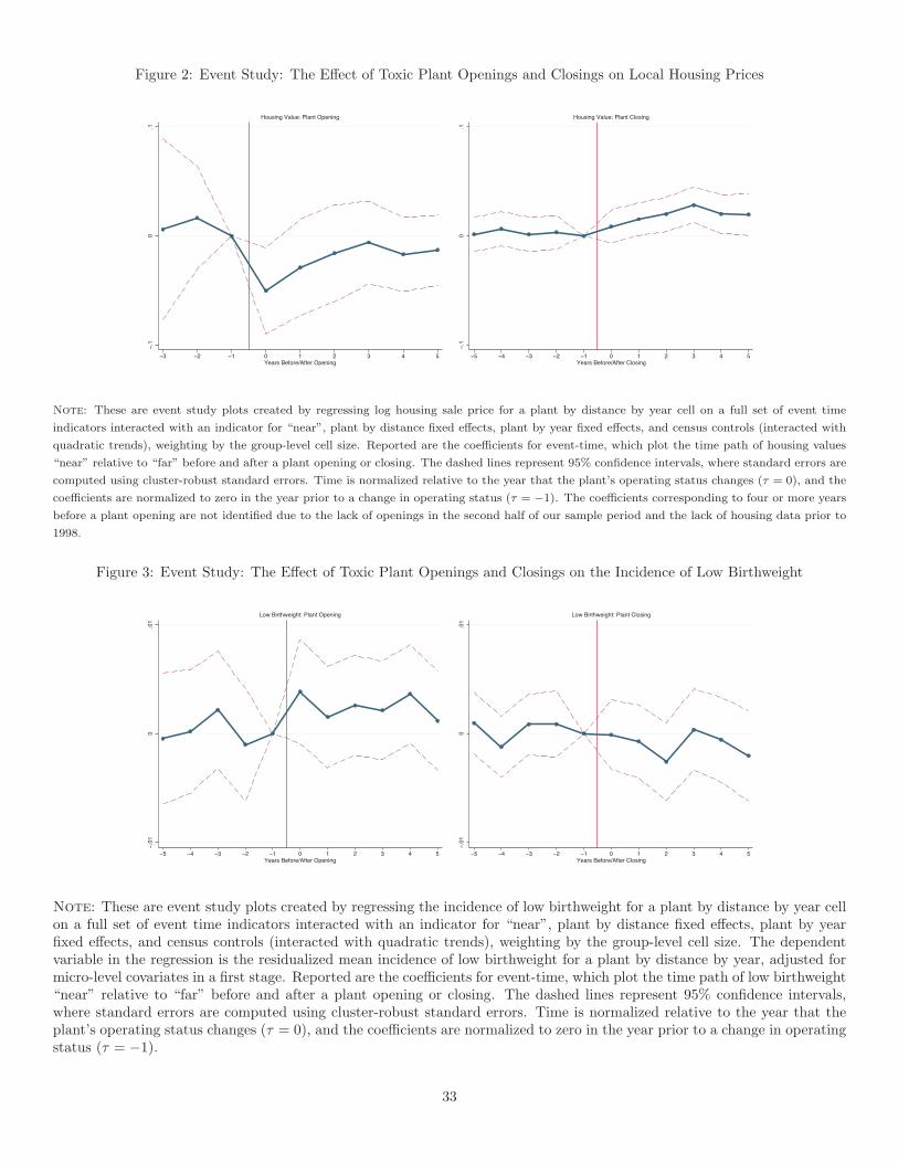
Figure 2: Event Study: The Effect of Toxic Plant Openings and Closings on Local Housing Prices

−.1

0.1

−3 −2 −1 0 1 2 3 4 5Years Before/After Opening

Housing Value: Plant Opening

−.1

0.1

−5 −4 −3 −2 −1 0 1 2 3 4 5Years Before/After Closing

Housing Value: Plant Closing

Note: These are event study plots created by regressing log housing sale price for a plant by distance by year cell on a full set of event time

indicators interacted with an indicator for “near”, plant by distance fixed effects, plant by year fixed effects, and census controls (interacted with

quadratic trends), weighting by the group-level cell size. Reported are the coefficients for event-time, which plot the time path of housing values

“near” relative to “far” before and after a plant opening or closing. The dashed lines represent 95% confidence intervals, where standard errors are

computed using cluster-robust standard errors. Time is normalized relative to the year that the plant’s operating status changes (τ = 0), and the

coefficients are normalized to zero in the year prior to a change in operating status (τ = −1). The coefficients corresponding to four or more years

before a plant opening are not identified due to the lack of openings in the second half of our sample period and the lack of housing data prior to

1998.

Figure 3: Event Study: The Effect of Toxic Plant Openings and Closings on the Incidence of Low Birthweight

−.0

10

.01

−5 −4 −3 −2 −1 0 1 2 3 4 5Years Before/After Opening

Low Birthweight: Plant Opening

−.0

10

.01

−5 −4 −3 −2 −1 0 1 2 3 4 5Years Before/After Closing

Low Birthweight: Plant Closing

Note: These are event study plots created by regressing the incidence of low birthweight for a plant by distance by year cellon a full set of event time indicators interacted with an indicator for “near”, plant by distance fixed effects, plant by yearfixed effects, and census controls (interacted with quadratic trends), weighting by the group-level cell size. The dependentvariable in the regression is the residualized mean incidence of low birthweight for a plant by distance by year, adjusted formicro-level covariates in a first stage. Reported are the coefficients for event-time, which plot the time path of low birthweight“near” relative to “far” before and after a plant opening or closing. The dashed lines represent 95% confidence intervals,where standard errors are computed using cluster-robust standard errors. Time is normalized relative to the year that theplant’s operating status changes (τ = 0), and the coefficients are normalized to zero in the year prior to a change in operatingstatus (τ = −1).

33

Tables

Table 1: Characteristics of Toxic Plants and the Surrounding Community

Panel A: Plant Characteristics by Opening and Closing Status

(1) (2) (3)

Open Continuously Opened Between Closed Between

1990-2002 1990 and 2002 1990 and 2002

Number of Plants 1846 689 1062Average Plant Employment (Total Workers) 224 90 114Average Plant Age (Years) 18.6 2.0 16.2Mean Value of Plant Equipment (in millions) $15.8 $15.4 $14.9Mean Value of Plant Structures (in millions) $6.2 $5.8 $5.1Mean Annual Salary and Wages (in millions) $11.7 $5.5 $6.2Mean Annual Toxic Emissions (in pounds) 22016 23303 17919

Panel B: Community Characteristics by Distance, d, from Plants that Opened or Closed 1990-2002

(1) (2) (3) (4)

0 < d ≤ 0.5 0.5 < d ≤ 1 0 < d ≤ 1 1 < d ≤ 2Housing Characteristics:

Mean Housing Value $124,424 $126,492 $125,927 $132,227Aggregate Housing Value (in millions) $38.56 $60.00 $98.57 $174.80

Birth and Maternal Characteristics:Mother’s Education 11.93 12.08 12.05 12.22Mother’s Age 26.33 26.50 26.46 26.70Proportion Teenage Mother 0.15 0.15 0.15 0.15Proportion Smoker 0.14 0.13 0.13 0.13Proportion African American 0.23 0.25 0.25 0.26Proportion Hispanic 0.32 0.30 0.31 0.29Proportion White/Caucasian 0.72 0.71 0.71 0.70

Notes: Panel A describes plants in Florida, Michigan, New Jersey, Pennsylvania, and Texas that reported to the ToxicRelease Inventory at least one year between 1990 and 2002. In calculating plant characteristics in columns (2) and (3), thesample is restricted to observations in the 2 years after a plant opening or 2 years before a plant closing to reflect meancharacteristics of an operating plant prior to “treatment”, and a single plant can appear in both columns. Plant age is rightcensored, as the the year a plant opened is not available for plants opened before 1975 in the Longitudinal Business Database.The value of plant equipment, structures, and salary and wages come from the NBER Productivity Database microdata andis only available for a subset of our data that matches the NBER Productivity Database in a given year. The value of plantequipment and structures is constructed using the perpetual inventory method from investment data (Mohr and Gilbert,1996). All dollar amounts are in 2000 dollars. Panel B statistics describe community characteristics surrounding toxic plantsthat either opened or closed between 1990 and 2002. Housing sales and births may appear in multiple columns if they arewithin 2 miles of more than one plant opening or closing, but within each column a house or birth appears only once.

34

Tab

le2:

The

Effec

tof

Tox

icP

lants

onLoca

lH

ousi

ng

Val

ues

0-0.

5M

iles

0.5-

1M

iles

0-1

Miles

0-1

Miles

(+/-

2yea

rs)

(1)

(2)

(3)

(4)

(5)

(6)

(7)

(8)

PanelA

:Esti

mate

dEffect

ofP

lant

Operati

on

1(P

lant

Oper

atin

g)by

Nea

r-0

.030

∗∗∗

-0.0

22∗∗∗

-0.0

10∗∗

-0.0

12∗∗∗

-0.0

15∗∗∗

-0.0

14∗∗∗

-0.0

09∗∗

-0.0

10∗∗∗

(0.0

07)

(0.0

06)

(0.0

05)

(0.0

04)

(0.0

05)

(0.0

04)

(0.0

04)

(0.0

03)

N34

736

3473

634

736

3473

634

736

34736

30492

30492

Pla

nt

Cou

nt

2171

2171

2171

2171

2171

2171

2171

2171

PanelB

:Esti

mate

dEffect

ofP

lant

Openin

gs

and

Clo

sin

gs

1(P

lant

Open

ed)

by

Nea

r-0

.012

-0.0

240.

007

-0.0

06-0

.002

-0.0

15

-0.0

10

-0.0

16

(0.0

21)

(0.0

15)

(0.0

15)

(0.0

12)

(0.0

14)

(0.0

11)

(0.0

12)

(0.0

12)

1(P

lant

Clo

sed)

by

Nea

r0.

031∗∗∗

0.02

2∗∗∗

0.01

0∗∗

0.01

2∗∗∗

0.01

5∗∗∗

0.0

14∗∗∗

0.0

09∗

∗0.0

09∗∗∗

(0.0

07)

(0.0

06)

(0.0

05)

(0.0

04)

(0.0

05)

(0.0

04)

(0.0

05)

(0.0

04)

H0:

Open

ing=

Clo

sing

(p-v

alue)

0.39

0.88

0.27

0.67

0.37

0.9

60.9

70.5

9

N34

736

3473

634

736

3473

634

736

34736

30492

30492

Pla

nt

Cou

nt

2171

2171

2171

2171

2171

2171

2171

2171

Pla

nt

by

Dis

tance

-Bin

FE

XX

XX

XX

XX

Sta

teby

Yea

rFE

XX

XX

Pla

nt

by

Yea

rFE

XX

XX

Notes:

This

table

repor

tsre

gres

sion

coeffi

cien

tsfr

om16

separ

ate

regr

essi

ons,

8per

pan

el.

The

dep

enden

tva

riable

inall

regre

ssio

ns

ishousi

ng

valu

es(i

nlo

gs),

and

the

dat

ahav

ebee

nag

greg

ated

topla

nt

by

dis

tance

by

year

cells.

Bot

hth

ere

gres

sion

sam

ple

and

the

indic

ato

rva

riable

“N

ear”

change

as

one

mov

esac

ross

the

colu

mns,

indic

ated

by

the

colu

mn

hea

din

gs.

For

exam

ple

,th

esp

ecifi

cati

onin

colu

mns

(1)

and

(2)

exam

ines

how

gro

up-lev

elav

erage

housi

ng

pri

ces

wit

hin

0.5

miles

ofa

pla

nt

(i.e

.“N

ear”

)re

spon

dto

pla

nt

oper

atin

gst

atus,

rela

tive

toth

eco

mpar

ison

gro

up.

The

com

pari

son

gro

up

inall

colu

mns

ishom

esbet

wee

n1

and

2m

iles

from

apla

nt.

Inco

lum

ns

(7)

and

(8),

the

sam

ple

rem

oves

obse

rvat

ions

mor

eth

an

two

years

bef

ore

and

aft

erch

anges

inpla

nt

acti

vity.

Pan

elA

repor

tses

tim

ates

ofth

eeff

ect

ofpla

nt

oper

atin

gst

atus

onlo

calhou

sing

valu

es,w

her

e1(P

lant

Oper

ati

ng)

isa

indic

ato

rva

riable

equalto

one

for

pla

nts

that

hav

eop

ened

and/o

rhav

enot

yet

clos

ed.

Pan

elB

repor

tses

tim

ates

ofth

eas

ym

met

ric

effec

tofpla

nt

open

ings/

closi

ngs.

Panel

Bre

port

sp-v

alues

from

test

sth

atth

etw

oco

effici

ents

are

equal

,but

ofop

pos

ite

sign

.A

llco

lum

ns

contr

olfo

rce

nsu

str

act

chara

cter

isti

cs(i

nte

ract

edw

ith

quadra

tic

tren

ds)

.R

egre

ssio

ns

are

wei

ghte

dby

the

grou

p-lev

elce

llsi

ze.

Sta

ndar

der

rors

two-

way

clust

ered

by

pla

nt

and

year

are

inpare

nth

eses

.

35

Table 3: The Effect of Toxic Plants on Local Housing Values: Heterogeneity Based on Median Plant Characteristics

(1a) (1b) (2a) (2b)

Employment Employment Payroll Payroll

< (p50) >= (p50) < (p50) >= (p50)

1(Plant Operating)×Near -0.008 -0.021∗∗ -0.006 -0.023∗

(0.007) (0.010) (0.006) (0.013)

N 20464 20544 19888 19952

PlantCount 1279 1284 1243 1247

(3a) (3b) (4a) (4b)

Fug. Emissions Fug. Emissions Stack Emissions Stack Emissions

< (p50) >= (p50) < (p50) >= (p50)

1(Plant Operating)×Near -0.003 -0.022∗∗∗ -0.018∗ -0.008

(0.008) (0.007) (0.010) (0.006)

N 14480 14480 14480 14480

Plant Count 905 905 905 905

(5a) (5b) (6a) (6b)

Mean Toxicity Mean Toxicity Max Toxicity Max Toxicity

< (p50) >= (p50) < (p50) >= (p50)

1(Plant Operating)×Near -0.004 -0.023∗∗∗ -0.014 -0.010

(0.009) (0.008) (0.011) (0.014)

N 9680 10192 13920 14272

Plant Count 605 637 870 892

Notes: This table reports regression coefficients from 12 separate regressions, where the respective (a) and (b) columns

stratify the sample by whether the plant-level median of the column variable (taken over plant operating years) is above or

below the sample median value (taken over median plant values). The dependent variable in all regressions is housing values

(in logs), and the data have been aggregated to plant by distance by year cells. The indicator variable “Near” is the same

across columns and is equal to 1 for all homes within one mile of a plant. All regressions control for plant by distance-bin and

plant by year fixed effects, and census tract characteristics (interacted with quadratic trends), and regressions are weighted

by the group-level cell size. The number of plants varies across regressions because emissions and/or toxicity data are not

available for all plants. Standard errors are two-way clustered by plant and year.

36

Tab

le4:

The

Effec

tof

Tox

icP

lants

onLow

Bir

thw

eigh

t

0-0.

5M

iles

0.5-

1M

iles

0-1

Miles

0-1

Miles

(+/-

2yea

rs)

(1)

(2)

(3)

(4)

(5)

(6)

(7)

(8)

PanelA

:Esti

mate

dEffect

ofP

lant

Operati

on

1(P

lant

Oper

atin

g)×

Nea

r0.

0010

0.00

120.

0014

∗∗

0.00

15∗∗

0.00

13∗∗

0.0

014∗

∗0.0

021∗

∗0.0

026∗∗∗

(0.0

010)

(0.0

012)

(0.0

006)

(0.0

006)

(0.0

006)

(0.0

007)

(0.0

009)

(0.0

009)

N88

958

8895

888

958

8895

888

958

88958

63324

63324

Pla

nt

Cou

nt

3438

3438

3438

3438

3438

3438

3438

3438

PanelB

:Esti

mate

dEffect

ofP

lant

Openin

gs

and

Clo

sin

gs

1(P

lant

Open

ed)×

Nea

r0.

0025

0.00

220.

0024

∗∗∗

0.00

27∗∗∗

0.00

24∗∗

0.0

024∗

∗∗

0.0

031∗

0.0

037∗∗

(0.0

019)

(0.0

018)

(0.0

009)

(0.0

010)

(0.0

009)

(0.0

008)

(0.0

017)

(0.0

017)

1(P

lant

Clo

sed)×

Nea

r-0

.000

2-0

.000

7-0

.000

9-0

.000

9-0

.000

7-0

.0009

-0.0

016

-0.0

021∗

(0.0

016)

(0.0

016)

(0.0

009)

(0.0

010)

(0.0

009)

(0.0

009)

(0.0

012)

(0.0

013)

H0:

Open

ing=

Clo

sing

(p-v

alue)

0.44

0.56

0.32

0.28

0.22

0.2

40.5

10.4

8N

8895

888

958

8895

888

958

8895

888958

63324

63324

Pla

nt

Cou

nt

3438

3438

3438

3438

3438

3438

3438

3438

Pla

nt×

Dis

tance

-Bin

FE

XX

XX

XX

XX

Sta

te×

Yea

rFE

XX

XX

Pla

nt×

Yea

rFE

XX

XX

Notes:

This

table

repor

tsre

gres

sion

coeffi

cien

tsfr

om16

separ

ate

regr

essi

ons,

8per

pan

el.

The

dep

enden

tva

riable

inall

regre

ssio

ns

isth

em

ean

inci

den

ceof

low

bir

thw

eigh

tw

her

eth

edat

ahav

ebee

nag

greg

ated

topla

nt

by

dis

tance

by

year

cells.

Cel

lle

velav

erag

eshav

ebee

nadju

sted

for

mate

rnalch

ara

cter

isti

csin

cludin

gag

e,ed

uca

tion

,ra

ce,an

dsm

okin

gbeh

avio

r,as

wel

las

for

mon

thof

bir

th,bir

thor

der

,an

dge

nder

ofch

ild.

See

text

for

det

ails.

The

mea

nin

ciden

ceof

low

bir

thw

eigh

tin

our

sam

ple

is0.

07.

Bot

hth

ere

gres

sion

sam

ple

and

the

indic

ator

vari

able

“Nea

r”ch

ange

as

one

mov

esacr

oss

the

colu

mns,

indic

ate

dby

the

colu

mn

hea

din

gs.

For

exam

ple

,th

esp

ecifi

cati

onin

colu

mns

(1)

and

(2)

exam

ines

how

grou

p-lev

elav

erage

bir

thoutc

om

esw

ithin

0.5

miles

ofa

pla

nt

(i.e

.“N

ear”

)re

spon

dto

pla

nt

oper

atin

gst

atus,

rela

tive

toth

eco

mpar

ison

grou

p.

The

com

par

ison

grou

pin

all

colu

mns

isbir

ths

bet

wee

n1

and

2m

iles

from

apla

nt.

Inco

lum

ns

(7)

and

(8),

the

sam

ple

rem

oves

obse

rvat

ions

mor

eth

antw

oyea

rsbef

ore

and

afte

rch

anges

inpla

nt

act

ivity.

Panel

Aes

tim

ate

sth

eeff

ect

ofpla

nt

oper

atin

gst

atus

onlo

calbir

thou

tcom

es,w

her

e1(

Pla

nt

Oper

atin

g)is

ain

dic

ator

vari

able

equal

toone

for

pla

nts

that

hav

eopen

edand/or

hav

enot

yet

clos

ed.

Pan

elB

esti

mat

esth

eas

ym

met

ric

effec

tof

pla

nt

open

ings

/clo

sings

.Pan

elB

repor

tsp-v

alues

from

test

sth

at

the

two

coeffi

cien

tsare

equal

inm

agnit

ude

but

ofop

pos

ite

sign

.A

llco

lum

ns

contr

olfo

rce

nsu

str

act

char

acte

rist

ics

(inte

ract

edw

ith

quad

rati

ctr

ends)

and

regre

ssio

ns

are

wei

ghte

dby

the

grou

p-lev

elce

llsi

ze.

Mult

iple

bir

ths

are

dro

pped

from

regr

essi

ons.

Sta

ndar

der

rors

are

two-

way

clust

ered

by

pla

nt

and

year.

37

Table 5: The Effect of Toxic Plants on Low Birthweight: Heterogeneity Based on Median Plant Characteristics

(1a) (1b) (2a) (2b)

Employment Employment Payroll Payroll

< (p50) >= (p50) < (p50) >= (p50)

1(Plant Operating)×Near 0.0016∗∗ 0.0007 0.0012 0.0015

(0.0007) (0.0011) (0.0007) (0.0012)

N 44274 44451 44207 44311

PlantCount 1712 1717 1709 1712

(3a) (3b) (4a) (4b)

Fug. Emissions Fug. Emissions Stack Emissions Stack Emissions

< (p50) >= (p50) < (p50) >= (p50)

1(Plant Operating)×Near 0.0010 0.0015 0.0007 0.0018∗∗

(0.0011) (0.0010) (0.0010) (0.0009)

N 39025 39104 39075 39054

Plant Count 1508 1511 1509 1510

(5a) (5b) (6a) (6b)

Mean Toxicity Mean Toxicity Max Toxicity Max Toxicity

< (p50) >= (p50) < (p50) >= (p50)

1(Plant Operating)×Near 0.0014 0.0012 0.0008 0.0026∗∗∗

(0.0010) (0.0014) (0.0010) (0.0010)

N 30486 30537 35789 38559

Plant Count 1178 1180 1383 1490

Notes: This table reports regression coefficients from 12 separate regressions, where the respective (a) and (b) columns

stratify the sample by whether the plant-level median of the column variable (taken over plant operating years) is above

or below the sample median value (taken over median plant values). The dependent variable in all regressions is the mean

incidence of low birthweight, where the data have been aggregated to plant by distance by year cells. The indicator variable

“Near” is the same across columns and is equal to 1 for all births within one mile of a plant. Cell level averages have been

adjusted for micro covariates, and all regressions control for plant by distance and plant by year fixed effects, as well as census

tract characteristics (interacted with quadratic trends). Regressions are weighted by the group-level cell size. The number

of plants varies across regressions because emissions and/or toxicity data are not available for all plants. Standard errors

two-way clustered by plant and year.

38

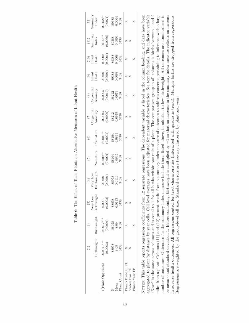
Tab

le6:

The

Effec

tof

Tox

icP

lants

onA

lter

nat

ive

Mea

sure

sof

Infa

nt

Hea

lth

(1)

(2)

(3)

(4)

(5)

(6)

(7)

(8)

(9)

(10)

(11)

(12)

Very

Low

Very

Low

Congenital

Congenital

Infa

nt

Infa

nt

Sum

mary

Sum

mary

Bir

thw

eig

ht

Bir

thw

eig

ht

Bir

thw

eig

ht

Bir

thw

eig

ht

Pre

matu

reP

rem

atu

reA

nom

aly

Anom

aly

Death

Death

Index

Index

1(P

lant

Op)×

Near

-0.0

011∗∗∗

-0.0

012∗∗∗

0.0

001

0.0

001

0.0

009∗∗

0.0

009∗∗

-0.0

003

-0.0

005

0.0

001

0.0

000

0.0

165∗∗

0.0

158∗∗

(0.0

003)

(0.0

004)

(0.0

002)

(0.0

001)

(0.0

004)

(0.0

005)

(0.0

009)

(0.0

010)

(0.0

001)

(0.0

001)

(0.0

066)

(0.0

071)

N88958

88958

88958

88958

88404

88404

88212

88212

89388

89388

89388

89388

Mean

8.0

98.0

90.0

113

0.0

113

0.0

845

0.0

845

0.0

679

0.0

679

0.0

068

0.0

068

-0.0

004

-0.0

004

Pla

nt

Count

3438

3438

3438

3438

3438

3438

3438

3438

3438

3438

3438

3438

Pla

nt×

Dis

t-B

inFE

XX

XX

XX

XX

XX

XX

Sta

te×

Year

FE

XX

XX

XX

Pla

nt×

Year

FE

XX

XX

XX

Notes:

This

table

repor

tsre

gres

sion

coeffi

cien

tsfr

om12

separ

ate

regr

essi

ons.

The

dep

enden

tva

riab

leis

list

edin

the

colu

mn

hea

din

g,and

data

hav

ebee

nag

greg

ated

topla

nt

by

dis

tance

by

year

cells.

Cel

lle

velav

erag

eshav

ebee

nad

just

edfo

rm

ater

nal

char

acte

rist

ics.

See

text

for

det

ails.

The

indic

ato

rva

riable

“Nea

r”is

the

sam

eac

ross

colu

mns

and

iseq

ual

to1

for

allbir

ths

wit

hin

one

mile

ofa

pla

nt.

The

com

par

ison

gro

up

inall

colu

mns

isbir

ths

bet

wee

n1

and

2m

iles

from

apla

nt.

Col

um

ns

(11)

and

(12)

pre

sent

resu

lts

from

asu

mm

ary

index

mea

sure

ofou

tcom

esto

addre

ssco

nce

rns

per

tain

ing

toin

fere

nce

wit

ha

larg

enum

ber

ofou

tcom

es.

Outc

omes

for

the

sum

mar

yin

dex

mea

sure

incl

ude

thos

elist

edab

ove,

inad

dit

ion

tolo

wbir

thw

eight.

All

outc

om

esare

standard

ized

tobe

mea

n0

and

stan

dar

ddev

iati

on1.

Bef

ore

com

bin

ing,

bir

thw

eigh

tis

mult

iplied

by−

1so

that

anin

crea

sein

the

sum

mary

index

mea

sure

reflec

tsan

incr

ease

inad

vers

ehea

lth

outc

omes

.A

llre

gres

sion

sco

ntr

olfo

rtr

act

char

acte

rist

ics

(inte

ract

edw

ith

quad

rati

ctr

end).

Mult

iple

bir

ths

are

dro

pped

from

regre

ssio

ns.

Reg

ress

ions

are

wei

ghte

dby

the

grou

p-lev

elce

llsi

ze.

Sta

ndar

der

rors

are

two-

way

clust

ered

by

pla

nt

and

year.

39

Tab

le7:

The

Effec

tof

Tox

icP

lants

onM

ater

nal

Char

acte

rist

ics

(1)

(2)

(3)

(4)

(5)

(6)

(7)

(8)

Afr

ican

Afr

ican

Mot

her

’sM

oth

er’s

Tee

nage

Tee

nage

Am

eric

anA

mer

ican

His

pan

icH

ispan

icE

duca

tion

Educa

tion

Moth

erM

oth

er

1(P

lant

Oper

atin

g)×

Nea

r-0

.007

∗∗∗

-0.0

06∗∗∗

-0.0

02-0

.001

0.00

80.0

01

-0.0

01

-0.0

00

(0.0

02)

(0.0

02)

(0.0

02)

(0.0

02)

(0.0

10)

(0.0

09)

(0.0

01)

(0.0

01)

N88

062

8806

287

438

8743

882

608

82608

89302

89302

Pla

ntC

ount

3438

3438

3438

3438

3438

3438

3438

3438

Mea

n0.

201

0.20

10.

219

0.21

912

.555

12.5

55

0.1

37

0.1

37

(9)

(10)

(11)

(12)

(13)

(14)

(15)

(16)

Whit

eW

hit

eP

redic

tive

Pre

dic

tive

Sm

oker

Sm

oker

Col

lege

Col

lege

Index

Index

Fer

tility

Fer

tility

1(P

lant

Oper

atin

g)×

Nea

r-0

.001

0.00

20.

002∗

∗0.

001

0.00

1∗∗∗

0.0

01∗

∗∗

0.0

02

-0.0

00

(0.0

01)

(0.0

01)

(0.0

01)

(0.0

01)

(0.0

00)

(0.0

00)

(0.0

05)

(0.0

04)

N88

077

8807

786

093

8609

389

388

89388

89388

89388

Pla

ntC

ount

3438

3438

3438

3438

3438

3438

3438

3438

Mea

n0.

149

0.14

90.

151

0.15

18.

084

8.0

84

4.2

33

4.2

33

Pla

nt×

Dis

tance

-Bin

FE

XX

XX

XX

XX

Sta

te×

Yea

rFE

XX

XX

Pla

nt×

Yea

rFE

XX

XX

Notes:

This

table

repor

tsre

gres

sion

coeffi

cien

tsfr

om16

separ

ate

regr

essi

ons,

8per

pan

el.

The

dep

enden

tva

riable

islist

edin

the

colu

mn

hea

din

g,and

data

hav

ebee

nag

greg

ated

topla

nt

by

dis

tance

by

yea

rce

lls.

Cel

lle

velav

erag

eshav

ebee

nad

just

edfo

rm

ater

nal

chara

cter

isti

cs.

See

text

for

det

ails.

The

indic

ato

rva

riab

le“N

ear”

isth

esa

me

acro

ssco

lum

ns

and

iseq

ual

to1

for

allbir

ths

wit

hin

one

mile

ofa

pla

nt.

The

com

pari

son

gro

up

inall

colu

mns

isbir

ths

bet

wee

n1

and

2m

iles

from

apla

nt.

The

dep

enden

tva

riab

le“P

redic

tive

Index

”is

crea

ted

by

firs

tru

nnin

ga

regr

essi

onofbir

thw

eight

on

obse

rvable

chara

cter

isti

csofth

em

other

.T

he

pre

dic

ted

valu

esfr

omth

isre

gres

sion

are

use

das

asu

mm

ary

index

ofdem

ogra

phic

chan

ges.

Fer

tility

ism

easu

red

as

the

log

num

ber

ofbir

ths

ina

cell.

Reg

ress

ions

are

wei

ghte

dby

the

grou

p-lev

elce

llsi

ze(w

ith

the

exce

pti

onof

“Fer

tility

”).

All

regr

essi

ons

contr

olfo

rtr

act

chara

cter

isti

cs(e

xcl

udin

gth

edep

enden

tva

riab

leof

inte

rest

),in

tera

cted

wit

hquad

rati

ctr

ends.

Mult

iple

bir

ths

are

dro

pped

from

regr

essi

ons.

Reg

ress

ions

are

wei

ghte

dby

the

gro

up-lev

elce

llsi

ze.

Sta

ndar

der

rors

two-

way

clust

ered

by

pla

nt

and

year

.

40

A Appendix Tables: Not For Publication

A1

Tab

leA

1:T

he

Effec

tof

Tox

icP

lants

onLoca

lH

ousi

ng

Val

ues

and

Low

Bir

thw

eigh

t:U

sing

2-4

Mile

Radiu

sC

om

pari

son

Gro

up

0-0.

5M

iles

0.5-

1M

iles

0-1

Miles

0-1

Miles

(+/-

2yea

rs)

(1)

(2)

(3)

(4)

(5)

(6)

(7)

(8)

PanelA

:Esti

mate

dEffect

ofP

lant

Operati

on

on

Housin

gV

alu

es

1(P

lant

Oper

atin

g)×

Nea

r-0

.032

∗∗∗

-0.0

26∗∗∗

-0.0

13∗∗

-0.0

17∗∗∗

-0.0

18∗∗∗

-0.0

19∗∗∗

-0.0

11∗

-0.0

12∗∗∗

(0.0

09)

(0.0

08)

(0.0

07)

(0.0

06)

(0.0

07)

(0.0

06)

(0.0

06)

(0.0

05)

N34

736

3473

634

736

3473

634

736

34736

30492

30492

Pla

ntC

ount

2171

2171

2171

2171

2171

2171

2171

2171

PanelB

:Esti

mate

dEffect

ofP

lant

Operati

on

on

Low

Bir

thw

eig

ht

1(P

lant

Oper

atin

g)×

Nea

r0.

0001

-0.0

000

0.00

09∗

0.00

11∗∗

0.00

070.0

008

0.0

017∗

∗0.0

020∗

∗∗

(0.0

011)

(0.0

011)

(0.0

006)

(0.0

005)

(0.0

006)

(0.0

005)

(0.0

008)

(0.0

008)

N88

922

8892

288

922

8892

288

922

88922

63301

62984

Pla

ntC

ount

3438

3438

3438

3438

3438

3438

3438

3438

Pla

nt×

Dis

tance

-Bin

FE

XX

XX

XX

XX

Sta

te×

Yea

rFE

XX

XX

Pla

nt×

Yea

rFE

XX

XX

Notes:

This

table

repor

tsre

gres

sion

coeffi

cien

tsfr

om16

separ

ate

regr

essi

ons,

8per

pan

el.

The

dep

enden

tva

riable

inPanel

Ais

housi

ng

valu

es(i

nlo

gs)

,and

the

dep

enden

tva

riab

lein

Pan

elB

isth

em

ean

inci

den

ceof

low

bir

thw

eigh

t.T

he

dat

ahav

ebee

nag

greg

ated

topla

nt

by

dis

tance

by

year

cells,

and

inPanel

Bhav

ebee

nad

just

edfo

rm

ater

nal

char

acte

rist

ics.

The

mea

nin

ciden

ceof

low

bir

thw

eigh

tin

our

sam

ple

is0.0

7.

Both

the

regre

ssio

nsa

mple

and

the

indic

ato

rva

riab

le“N

ear”

chan

geas

one

mov

esac

ross

the

colu

mns,

indic

ated

by

the

colu

mn

hea

din

gs.

For

exam

ple

,th

esp

ecifi

cati

on

inco

lum

ns

(1)

and

(2)

exam

ines

how

grou

p-lev

elou

tcom

esw

ithin

0.5

miles

ofa

pla

nt

(i.e

.“N

ear”

)re

spon

dto

pla

nt

oper

atin

gst

atus,

rela

tive

toa

com

pari

son

gro

up.

The

com

pari

son

gro

up

inal

lco

lum

ns

isob

serv

atio

ns

bet

wee

n2

and

4m

iles

from

apla

nt.

Inco

lum

ns

(7)

and

(8),

the

sam

ple

rem

oves

obse

rvati

ons

more

than

two

years

bef

ore

and

afte

rch

ange

sin

pla

nt

acti

vity.

All

regr

essi

ons

contr

olfo

rce

nsu

str

act

char

acte

rist

ics

(inte

ract

edw

ith

quad

rati

ctr

ends)

,and

regre

ssio

ns

are

wei

ghte

dby

the

grou

p-lev

elce

llsi

ze.

Mult

iple

bir

ths

are

dro

pped

from

the

regr

essi

ons

inPan

elB

.Sta

ndar

der

rors

are

two-

way

clust

ered

by

pla

nt

and

year.

A2

Table

A2:

The

Effec

tofToxic

Pla

nts

on

Loca

lH

ousi

ng

Pri

ces

and

Low

Bir

thw

eight,

Dis

tance

Radiu

sSpec

ifica

tion

(1)

(2)

(3)

(4)

(5)

(6)

(7)

(8)

(9)

(10)

(11)

(12)

0-0

.50-0

.50.5

-10.5

-11-1

.51-1

.51.5

-21.5

-20-1

0-1

1-2

1-2

PanelA

:Esti

mate

dEffect

ofP

lant

Operati

on

on

Housin

gV

alu

es

1(P

lant

Oper

ati

ng)

-0.0

18∗∗

-0.0

18∗∗

-0.0

11

-0.0

13∗

-0.0

02

-0.0

06

0.0

04

-0.0

00

-0.0

15∗∗

-0.0

16∗∗

0.0

00

-0.0

03

(0.0

09)

(0.0

08)

(0.0

07)

(0.0

07)

(0.0

06)

(0.0

07)

(0.0

06)

(0.0

06)

(0.0

07)

(0.0

07)

(0.0

06)

(0.0

06)

N17336

17336

17368

17368

17368

17368

15976

15976

17368

17368

17368

17368

Pla

ntC

ount

2167

2167

2171

2171

2171

2171

1997

1997

2171

2171

2171

2171

PanelB

:Esti

mate

dEffect

ofP

lant

Operati

on

on

Low

Bir

thw

eig

ht

1(P

lant

Oper

ati

ng)

0.0

004

0.0

003

0.0

012∗∗

0.0

012∗∗

-0.0

012∗

-0.0

012∗

-0.0

003

-0.0

002

0.0

009

0.0

009

-0.0

003

-0.0

003

(0.0

011)

(0.0

012)

(0.0

005)

(0.0

005)

(0.0

007)

(0.0

007)

(0.0

004)

(0.0

005)

(0.0

006)

(0.0

006)

(0.0

003)

(0.0

003)

N42077

42077

42140

42140

42114

42114

40556

40556

74890

74890

75002

75002

Pla

ntC

ount

3254

3254

3256

3256

3256

3256

3136

3136

5787

5787

5794

5794

Pla

nt

FE

XX

XX

XX

XX

XX

XX

Yea

rFE

XX

XX

XX

Sta

te×

Yea

rFE

XX

XX

XX

Notes:

This

table

report

sre

gre

ssio

nco

effici

ents

from

24

separa

tere

gre

ssio

ns,

12

per

panel

.T

he

dep

enden

tvari

able

inPanel

Ais

housi

ng

valu

es(i

nlo

gs)

,

and

the

dep

enden

tvari

able

inPanel

Bis

the

mea

nin

ciden

ceof

low

bir

thw

eight.

The

data

have

bee

naggre

gate

dto

pla

nt

by

dis

tance

by

yea

rce

lls,

and

in

Panel

Bhave

bee

nadju

sted

for

mate

rnalch

ara

cter

isti

cs.

The

mea

nin

ciden

ceoflo

wbir

thw

eight

inour

sam

ple

is0.0

7.

The

regre

ssio

nsa

mple

changes

as

one

moves

acr

oss

the

colu

mns,

indic

ate

dby

the

colu

mn

hea

din

gs.

For

exam

ple

,th

ees

tim

ate

dco

effici

ents

inco

lum

ns

(1)

and

(2)

corr

espond

toth

eeff

ect

ofpla

nt

oper

ati

ng

statu

sw

ithin

0.5

miles

of

apla

nt.

All

regre

ssio

ns

contr

ol

for

censu

str

act

chara

cter

isti

cs(i

nte

ract

edw

ith

quadra

tic

tren

ds)

,and

regre

ssio

ns

are

wei

ghte

dby

the

gro

up-lev

elce

llsi

ze.

Mult

iple

bir

ths

are

dro

pped

from

the

regre

ssio

ns

inPanel

B.Sta

ndard

erro

rsare

two-w

ay

clust

ered

by

pla

nt

and

yea

r.

A3