do macroeconomic factors defy the expected relationship

International Journal of Economics and Finance; Vol. 13, No. 10; 2021

ISSN 1916-971X E-ISSN 1916-9728

Published by Canadian Center of Science and Education

28

Do Macroeconomic Factors Defy the Expected Relationship with FDI

Inflows in a Developing Country? An Econometric Analysis Based on

Bangladesh

Sk. Riad Arefin1, Swarnil Roy

2 & Avijit Mallik

3

1 MBA Student, Institute of Business Administration, University of Dhaka, Bangladesh

2 Assistant Director, Bangladesh Bank, Dhaka, Bangladesh

3 Assistant Professor, Institute of Business Administration, University of Dhaka, Bangladesh

Correspondence: Swarnil Roy, Assistant Director, Bangladesh Bank, Dhaka, 53/1, Monir Hossain Lane, Narinda,

Dhaka-1100, Bangladesh. Tel: 880-168-448-2452. E-mail: [email protected]

Received: July 24, 2021 Accepted: August 27, 2021 Online Published: August 30, 2021

doi:10.5539/ijef.v13n10p28 URL: https://doi.org/10.5539/ijef.v13n10p28

Abstract

Through econometric analysis, this study investigates the effects of various economic factors on foreign direct

investment (FDI) inflows in Bangladesh from 1980 to 2019. ARDL (Autoregressive Distributed Lag) has been

used to estimate the economic determinants of FDI inflows in Bangladesh after removing the trends from the

independent variables. Empirical results revealed that GDP, Fixed Telephone Subscribers, Inflation Rate, and

Education Spending are the eminent economic determinants of FDI. Subsequently, a Granger causality test and

Vector Auto Regression (VAR) confirmed the absence of any long-term impact of these variables on FDI. From the

analysis, it is evident that the ADF (Augmented Dickey-Fuller) test is necessary to remove the trend from these

variables and corner those variables for the ARDL method to find the significant ones that have substantial impacts

on FDI in Bangladesh. GDP, Fixed Telephone Subscribers, Inflation Rate, and Education Spending are found to be

statistically significant while all of them having a positive impact on the FDI. Even though this study matches with

many other previous studies conducted by researchers, some exciting findings contradict the expected result and

open new doors for further research.

Keywords: Foreign Direct Investment, FDI in developing countries, Bangladesh, determinants of FDI,

econometrics, ARDL approach

1. Introduction

Foreign direct investment (FDI) has always been an influential factor in boosting a country‟s economic growth.

And, in the case of a developing nation, capitalizing on the potential to attract international investors would always

be a top priority due to the desperate need to maintain economic development. Bangladesh is not immune to this

phenomenon; ideally, historical datasets indicating a steady rise in FDI inflow over the years should be examined

with far more zeal than before to open new avenues for attracting FDI inflows, which would be critical in

strengthening the economic growth of a developing country like Bangladesh.

Since it establishes secure and long-lasting relations between economies, FDI is a critical component of

international economic integration. FDI facilitates the transfer of technology between countries, encourages

international trade by providing access to new markets, and can help countries grow economically (OECD). It can

be attributed to Bangladesh‟s massive rise in FDI inflows in recent decades, with a 412.93 percent increase in 2003.

Growth was satisfactory until 2014, but since then, the numbers have been deteriorating, which may harm the

economic growth, even though 2018 showed a 33.76 percent increase (Bank). With this backdrop, it is not

surprising that immense empirical literature has sprung up to investigate the forces attracting FDI (Chakrabarti,

2003).

Furthermore, the findings of this study have important implications for policymakers to determine where to focus

on attracting more FDI inflows into developing countries. The research would be critical in understanding the

significance of enhancing social and economic infrastructure, such as education and telecommunications, in

attracting foreign investors. Consequently, the impact of macroeconomic factors such as inflation rate, GDP, does

ijef.ccsenet.org International Journal of Economics and Finance Vol. 13, No.10; 2021

29

not appear to be as straightforward as found in earlier studies making the research findings novel. Instead, the

investigation provides several astounding findings that will add to previous discoveries so that policymakers will

reconsider their perspective on these variables influencing FDI.

Aside from that, it is critical to highlight the differences between this study and previous studies. We identified a

lack of effort made in earlier works on this topic in selecting variables and eradicating trends in those factors,

making previous findings somewhat unreliable as the accuracy of those investigations were compromised.

Furthermore, most studies relied on Ordinary Least Squares (OLS) Regression but did not provide sufficient

evidence to support the judgment. We believed that these studies could not capture the actual scenario of FDI

inflows into developing countries that would yield accurate results in evaluating determinants of FDI inflows. This

study went through a rigorous process of selecting independent variables to accomplish precise results. To remove

the trends from variables, we performed an ADF test. Furthermore, the research probes multicollinearity among

these factors in selecting appropriate variables from a long list of variables deemed in the first place. Section 3.1

will go into full depth regarding variable selection. Thus, the necessity for obtaining an appropriate methodology

with datasets free from biasedness holds a significant portion in our research works which is a key differentiator of

this study from previous works as well.

So, if the goal is to entice foreign investors in developing countries like Bangladesh, it is unavoidable to investigate

and comprehend the economic factors influencing FDI inflows. The analysis is focused on achieving that aim, and

every effort has been made to contribute to the findings of other researchers working on this topic. The empirical

evidence from previous studies is presented in the second section of this study. The third section goes over the

datasets and methodology, while the fourth section delves into the empirical findings and their implications.

2. Literature Review

Various types of research on the factors influencing FDI inflows have been supervised. Das and Das (2020)

conducted one such study. They used an econometric model in conjunction with statistical methods such as

correlation and regression to analyze 15 years of FDI inflow and other related factors in Bangladesh. GDP,

inflation rate, infrastructure level, trade openness, and labor cost productivity all have a strong positive relationship

with FDI inflow in Bangladesh, while political stability and tax rate have a strong negative relationship.

Adhikary and Mengistu (2018) investigated foreign direct investment inflows into South and Southeast Asian

economies. Over 27 years (1980-2006), they used data from 12 South and Southeast Asian countries. The paper

empirically explained the shocking disparity in FDI inflows among those countries based on key determinants

such as market size, per capita income growth, interest rate, exchange rate, human capital, and infrastructure.

Ahamed and Tanin (2011) strived to analyze the relationship between the FDI and World Development Indicators

and the impact of FDI on economic growth in Bangladesh based on time series data. Exports plus imports to GDP

ratio, industrial infrastructure, efficient wage rate, gross capital formation, foreign exchange reserve, electric

power consumption, and telecommunication subscribers were observed to have a significant positive relationship

with FDI inflows in this study. Furthermore, the researchers concluded that economic growth in a host country

would be responsible for FDI inflows rather than the traditional belief that FDI would yield economic growth.

Lewis (1997) showcased several determinants working behind the enticement of FDI in LDCs (Lesser Developed

Countries) with the current economic situation, past economic performance and solidity, the standard of human

capital, degree of trade restrictions, the steadiness of government, infrastructure level, and other varied factors in

an attempt to dig out the factors underlying FDI in LDCs. The experiment employed ordinary least squares

regression techniques to assess data from 157 developing countries. The literacy rate and the infrastructure level,

as reflected by the urbanization rate, were proven to have a greater effect on FDI inflow in LDCs, according to this

report.

Rahman (2012) attempted to give an impression of the FDI inflow towards Bangladesh in different sectors and

explore its prospects and challenges with the repercussions of FDI on the economy. Her methodology consisted of

an econometric model with several statistical tools such as trend analysis, standard deviations, and regression

analysis over 15 years (1996-2010). According to this research, cheap labor force, strategic location, regional

connectivity, local market growth, low energy cost, competitive incentive, export, and economic zones could work

as potential triggers for FDI inflow.

Rahman and Lau (2018) attempted to discern the determinants behind FDI by undertaking a comparative analysis

between two neighboring countries: India and Bangladesh. The research was analyzed using secondary data from

the World Bank and IMF over 25 years (1990-2014). To classify the determinants of FDI inflow in India and

Bangladesh, this research employed pattern analysis, descriptive statistics, and EViews to interpret the regression.


30

The research implied that market size quantified by population and GDP per capita had been significantly

associated with the FDI inflow both in Bangladesh and India whereas, in terms of infrastructure level measured by

telephone line users and trade openness expressed by exports plus imports as a share of GDP, India had been way

ahead of Bangladesh in attracting FDI inflow.

From 1981 to 2015, Shrivastava (2017) scrutinized various factors influencing FDI (Foreign Direct Investment) in

India. The factors‟ for the extensive assessment of FDI inflows were determined using a log-linear regression

model and least square methods, which were highly dependent on changes in Trade openness, indirect tax, FOREX,

external debt, government spending, and per capita electric consumptions.

Manzoor and Chowdhury (2016) investigated the factors influencing FDI inflows in Bangladesh using a functional

relationship with the dominant determinants of economic growth. Using time-series data from 1994 to 2014, they

ran four empirical models to examine the relationship between GDP, exports, imports, and domestic investments.

Encouraging FDI inflows could boost GDP growth while also improving the trade balance by lowering imports.

Even though their research was confined to a few industries, it was revealed that diversifying exports could be a

solution.

Similarly, Wijeweera and Mounter (2008) used the Vector Auto-Regressive (VAR) approach to evaluate

macroeconomic factors as inbound FDI increased by 10.9 percent in Sri Lanka by 2004. Dataset from 1950 to 2004

was used to dissect the previously chosen five crucial elements (market size and performance, openness indicator,

labor cost indicator, exchange rate, and interest rate) for detecting the correlation with FDI inflows to a country.

Ali et al. (2015) inspected the FDI-led growth hypothesis in Bangladesh using time series data from 1973 to 2013.

The researcher identified the relationship between FDI and growth using an econometric co-integration framework

and an error correction mechanism. To measure the relationships between GDP and FDI, ADF (Augmented

Dickey-Fuller) and Phillips-Perron (PP) tests with OLS (Ordinary Least Square) were included.

Hussain and Haque (2016) conducted a similar study in which they delineated the factors using the Vector Error

Correction Model (VECM) to find the interconnections between FDI, growth per capita GDP, and trade using time

series data from 1973 to 2014. The VECM findings confirmed a crucial relationship between these variables, in

which the residuals of the regression model could not find any auto-correlation, implying that governments must

pay close attention to the creation of trade-friendly investment.

Epaphra (2018) utilized datasets from 1996 to 2016 from 48 African countries to create a correlation between the

factors influencing FDI using the Random Effect (RE) model. The researcher also asserted that GDP per capita,

population growth, and economic openness could steer FDI inflows into a country. Political stability, government

effectiveness, corruption control, regulatory quality, and the rule of law were all factored into the logarithmic

regression models used in this study, along with the author‟s estimates. Political stability and corruption control

have a moderate relationship with FDI inflows at the 5% and 1% levels.

So, it‟s evident from almost all the studies that the GDP, or in other words, the market size of a country, is a

predominant factor in attracting FDI inflows in a country. However, to draw a line between the GDP of a current

and lagged period is necessary to comprehend the time-series relationship that GDP has with the FDI inflow in a

developing country which we have shown in our research. On the other hand, according to every further study and

ours, the social and economic infrastructures have a significantly positive relationship with FDI inflows in

developing countries like Bangladesh. Nonetheless, different researchers take distinct measurements of variables

in assessing infrastructure level, which in our study are telecommunications and education spending. Another

significant factor is the inflation rate which earlier studies drew a negative relationship with FDI inflows. But, that

wasn‟t the case in our research, which is indeed the most incredible insight derived from our investigation. In our

study, only a one-year lag in the inflation rate significantly impacts FDI inflows, and the relationship is

astonishingly positive. However, underlying depreciation in exchange rate with the rise in the inflation rate over

one year, which is the corresponding lagged period here, is the proper explanation behind this defying result as that

attracts foreign investors to invest at a lower cost in a developing country like Bangladesh. It is a noteworthy fact

for policymakers that our research reveals, which we believe is an excellent addition to the earlier studies on this

topic.

3. Data, Scope and Method

The data for FDI inflow in Bangladesh used in this study comes from secondary sources. There are some variables

assumed to have a congruent effect on FDI due to their relationship to GDP per capita; however, it is critical to

distinguish the truly effective factors that may have the potential to change FDI inflows in the country positively or

negatively. To analyze the effects, factors such as GDP, Inflation Rate, Lending Rate, Fixed Telephone Subscribers,


31

and Education Spending are retrieved from the other variables in a quantifiable form.

3.1 Variables Selection

In order to establish the effective prominent macroeconomic variables influencing FDI inflows we first filtered

through 13 variables. We noticed these variables can bolster the research if found in frequent manner. The

variables are listed in Table 1:

Table 1. Considered variables at first

Variables Notation Description Expected Effects

Independent

Variables

GDP GDP Per Capita (Income) +

GDP Growth Rate

Interest Rate Lending Rate -

Exchange Rate USD Conversion Rate +/-

INF Inflation Rate -

INFR Telecommunication +

Industry

TO (Trade Openness) Export Index +

Import Index -

Education Education Spending +

Trade Performance Export (% of GDP) +

Domestic Urban Population +/-

Final Consumption Expenditure

FOREX Reserve In terms of USD +

Note. In this table, we consider the variables which may have the major impacts on FDI inflows.

These variables are considered with a focus on possible macroeconomic determinants of FDI in a developing

country like Bangladesh such as income level, interest, inflation, exchange rate, etc. Besides that, factors such as

infrastructure level, education level, foreign trade, etc. were taken into consideration as well before delving into

further research. We used multicollinearity detection analysis in EViews to illuminate the best outcome from those

independent variables. Mulitcollinearity describes an exact relationship between the variables in the regression

exploratory analysis. Linear regression analysis is predicated on the notion that there is no perfect exact

relationship among exploratory variables. When independent variables in a regression model are correlated, the

problem of multicollinearity emerges. After fitting the model and interpreting the results, a high degree of

correlation between variables can lead to further complications. Any regression model with more than one

predictor can be affected by multicollinearity. It occurs when the measures of two or more predictor variables

overlap so much that their effects are indiscernible ((Complete Dissertation), (Frost)). Variable Inflation Factor

(VIF) is a tool to deduce the multicollinearity problem in a regression analysis. A large value in VIF on the

independent variables means high correlation while the smaller value depicts the reverse. In this analysis, we

factored all the variables to get the desired centered VIF results. After numerous simulations, we coalesced at a

certain point with five macro-economic variables (Table 2).

Table 2. Multicollinearity correction with VIF analysis

Variance Inflation Factors

Sample: 1980-2019

Coefficient Uncentered Centered

Variable Variance VIF VIF

LOGGDP(-1) 0.000396 134.9111 5.099472

LOGFIXEDTELEPHONESUBSCRIBERS 0.00033 1149.249 4.622253

LENDINGRATE 0.228114 393.7722 5.574866

LENDINGRATE(-1) 0.227142 393.3159 5.249071

INFLATIONRATE 0.009232 5.825832 1.290425

EDUCATIONSPENDING 0.002304 3.635354 1.239807

C 0.006196 674.154 NA

Note. In this table, we reduce the multicollinearity problem with VIF analysis. Value more 10 regards as a high correlation among the

independent variables in this research. Value between 1-5 indicates moderate correlation.


32

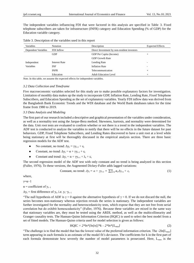
The independent variables influencing FDI that were factored in this analysis are specified in Table 3. Fixed

telephone subscribers are taken for infrastructure (INFR) category and Education Spending (% of GDP) for the

Education variable category.

Table 3. Description of the variables used in this report

Variables Notation Description Expected Effects

Dependent Variables FDI Inflow Direct Investment by non-resident investors

Independent

Variables

GDP GDP Per Capita (Income) +

GDP Growth Rate

Interest Rate Lending Rate -

INF Inflation Rate -

INFR Telecommunication +

Education Adult Education Level +

Note. In this table, we assume the expected effects for independent variables.

3.2 Data Collection and Timeframe

Five macroeconomic variables selected for this study are to make possible explanatory factors for investigation.

Limitation of monthly data makes up the study to incorporate GDP, Inflation Rate, Lending Rate, Fixed Telephone

Subscribers, and Education Spending as the set of explanatory variables. Yearly FDI inflow data was derived from

the Bangladesh Bank Economic Trends and the WDI database and the World Bank databases taken for the time

frame from 1980 to 2019.

3.3 Data Analysis and Modeling

The first part of our research included a descriptive and graphical presentation of the variables under consideration,

as well as a normality test using the Jarque-Bera method. Skewness, kurtosis, and normality were determined for

the data. Unit root tests are evaluated to confirm whether or not there is a trend in the independent variables. The

ADF test is conducted to analyze the variables to notify that there will be no effects in the future dataset for past

behaviors. GDP, Fixed Telephone Subscribers, and Lending Rates discovered to have a unit root at a level while

being stationary at first will be thoroughly discussed in the empirical analysis section. There are three basic

regression models for the ADF test.

No constant, no trend: Δyt = γyt-1 + εt

Constant, no trend: Δyt = α + γyt-1 + εt

Constant and trend: Δyt = α + γyt-1 + λt + εt

The second regression model of the ADF test with only constant and no trend is being analyzed in this section

(Fuller, 1976). To these versions, the Augmented Dickey-Fuller adds lagged variations:

Constant, no trend: Δyt = α + γyt-1 + ∑ 𝑎𝑚𝑠=1 sΔyt-s + εt (1)

where,

γ=α−1

α = coefficient of yt−1

Δyt = first difference of yt, i.e. yt−yt−1

“The null hypothesis of ADF is γ = 0 against the alternative hypothesis of γ < 0. If we do not discard the null, the

series becomes non-stationary whereas rejection reveals the series is stationary. The independent variables are

further investigated for the normality and heteroscedasticity tests, which expose that they are not free from serial

correlation but do exhibit homoscedasticity” (Fuller, 1976). Because these variables are mixed in the same way

that stationary variables are, they must be tested using the ARDL method, as well as the multicollinearity and

Granger causality tests. The Hannan-Quinn Information Criterion (HQIC) is used to select the best model from a

set of fitted models. The Hannan-Quinn criteria used for model selection is given as follows:

HQIC = 2*ln*[ln[n]]*k – 2*ln*[Lmax] (2)

“The challenge is to find the model that has the lowest value of the preferred information criterion. The -2ln[Lmax]

term appearing in each formula is an estimate of the model fit‟s deviance. The coefficients for k in the first part of

each formula demonstrate how severely the number of model parameters is prosecuted. Here, Lmax is the


33

lоg-likelihооd, number of parameters is indicated by k, and n denotes the number of observations” (Vose, 2017).

Because of the mixed variables, we incorporate ARDL approach which has been used for decades to simulate the

influence of economic variables in a single-equation time-series setup (Kripfganz & Schneider, September 7,

2018). “An autoregressive distributed lag (ARDL) model is an ordinary least squares (OLS) based approach that

can be applied to both non-stationary and mixed order of integration time series. This analysis supports sufficient

lags to capture the data generation process in a specific modeling framework. A simple linear evolution can also be

used to derive a vibrant error correction model (ECM) from ARDL. Correspondingly, the ECM merges short-run

dynamics with long-run equilibrium without risking long-run information and eliminates issues such as dubious

relationships associated with non-time series data” (Shrestha & Bhatta, 2018). In its most basic form, the ARDL

model is as follows:

yt = α + βxt + ζzt + εt (3)

The error correction version of the ARDL model is given by:

yt = α0 + ∑ 𝛽𝑝𝑖=1 iΔyt-i + ∑ 𝛿

𝑝𝑖=1 iΔxt-i + ∑ 휀

𝑝𝑖=1 iΔzt-i + 𝜆1yt-1 + 𝜆2xt-1 + 𝜆3zt-1 + μt (4)

“The short-run dynamics of the model are described by the first part of the equation with β, δ, and ε. The second

part with λs defines a long-term relationship. The null hypothesis in the equation is λ1 + λ2 + λ3 = 0, which refers

to the absence of a long-term relationship” (Shrestha & Bhatta, 2018).

“Since there is a bilateral condition among the variables due to the trend pattern, a Granger Causality test for these

independent variables and the dependent variable is expected. If two variables, Y and X, are co-integrated, then

either of the three relationships could occur: a) X affects Y, b) Y affects X, and c) X and Y affect both. The first two

resemble a one-way relationship, while the third conveys a two-way relationship. If two variables are not

co-integrated, they are autonomous and have no effect on each other. If the current and lagged values of X help

make accurate predictions of Y, then it is said that X „Granger causes‟ Y” (Buteikis, n.d.). The simple form of

Granger causality is as follows:

ΔYt = ∑ 𝛼𝑛𝑖=1 iΔYt-i + ∑ 𝛽𝑛

𝑗=1 jΔXt-j + μ1t (5)

ΔXt = ∑ 𝜆𝑛𝑖=1 iΔXt-i + ∑ 𝛿𝑛

𝑗=1 jΔYt-j + μ2t (6)

“The current value of ΔY is related to the past values of itself and the past values of ΔX. Similarly, ΔX is related to

the past values of itself and that of ΔY. The null hypothesis in equation 5 is βj = 0 which means, “ΔX does not

Granger cause ΔY”. Similarly, the null hypothesis in equation 6 is δj = 0 and states “ΔY does not Granger cause

ΔX.” The rejection or non-rejection of the null hypothesis is based on the F-statistics. The null hypothesis was

rejected for a value greater than the F-value” (Buteikis).

“To investigate the dynamic relationship between FDI inflows and macroeconomic variables, a Vector

AutoRegression (VAR) model is also used. To measure relationships between multiple variables over time, a

Vector Auto-regression (VAR) model is used. Using the dependent and independent repressors‟ past values, the

model allows feedback or reverses causality. Exogenous variables are not required in the general VAR model

because all repressors are assumed to be endogenous. Equation 7 & 8 are the simplified VAR dimension for two

variables X and Y with just one lag:

Yt = δ1 + θ11Yt-1 + θ12Xt-1 + γyt-1 + ε1t (7)

Xt = δ2 + θ12Yt-1 + θ22Xt-1 + γyt-1 + ε2t (8)

Where ε1t and ε2t are uncorrelated white noise disturbances or error terms. Choosing appropriate lag length is

important in VAR modeling. Optimal number of lags can be selected by using available lag length selection criteria.

Most popular criteria are Akaike Information Criterion (AIC), Schwarz Bayesian Criterion (SBC) and Hannan

Quinn criterion” (HQC) (Shrestha & Bhatta, 2018).

4. Empirical Results and Discussion

In this section, we briefly present our analysis of the data and discuss the findings from our modeling effort.

4.1 Descriptive Statistics and Graphical Presentation of the Data

If we look at the descriptive statistics, we can see that the average lending rate is around 12.5 percent. On the other

hand, over these 40 years, the average inflation rate was around 6.7 percent (1980-2019). For a developing country

like Bangladesh, the average education spending percentage of GDP is very low.

https://www.sciencedirect.com/topics/economics-econometrics-and-finance/akaike-information-criterion

https://www.sciencedirect.com/topics/economics-econometrics-and-finance/bayesian


34

Table 4. Descriptive analysis

LOGFDI LOGGDP LOGFIXEDTELEPH

ONESUBSCRIBERS

LENDINGRATE INFLATIONRATE EDUCATIONSPENDING

Mean 1.914338 1.77864 5.655328 0.125262 0.066643 0.097368

Median 2.266601 1.72981 5.721653 0.129108 0.06375 0.113052

Maximum 3.451963 2.480828 6.161263 0.148457 0.191432 0.204904

Minimum -0.60571 1.245736 4.977724 0.0954 0.001555 0

Std. Dev. 1.267103 0.358124 0.365008 0.015403 0.035955 0.072485

Skewness -0.36097 0.358697 -0.331221 -0.352036 1.657324 -0.272929

Kurtosis 1.714663 2.100933 1.808536 2.288642 6.945167 1.540579

Jarque-Bera 3.441024 2.094709 2.942492 1.586101 42.03945 3.844129

Probability 0.178974 0.350865 0.229639 0.452462 0 0.146305

Sum 72.74485 67.58833 214.9025 4.759953 2.532441 3.699974

Sum Sq. Dev. 59.40531 4.74536 4.929544 0.008778 0.047831 0.1944

Note. In this table, descriptive statistics are employed for investigation.

Following that, a normality test was performed to evaluate the pattern in the datasets. Except for the inflation rate,

the skewness and kurtosis of all other variables are close to zero and around three, indicating their normality.

However, to obtain a better result, a Jarque-Bera test was performed, in which the evidence of all variables was

normal except the inflation rate.

Figure 1 also shows a graphical representation of time plotting, where upward trends for some variables can be

seen. As a result, it became unavoidable for us to conduct Unit Root Tests and take the necessary steps to eliminate

all of those trends.

Figure 1. Time plots of the variables

4.2 Augmented Dickey-Fuller (ADF) Test (Level)

Table 5 displays summary results from Augmented Dickey-Fuller (ADF) tests for all variables. Appendix A

contains detailed results for each test, as well as t-statistics, R-squared, adjusted R-squared, and other test

parameters. The null hypothesis for FDI inflow was rejected at a significance level of 1%. The null hypothesis

could not be rejected for the remaining variables because the variables Log of GDP, Log of Fixed Telephone

Subscribers, and Lending Rate all have unit roots at the level. Because of this, a first difference unit root test for

these three variables was required.


35

Table 5. Summary results from the unit root test (at level)

LOGFDI LOGGDP LOGFIXEDTELEPHONE

SUBSCRIBERS

LENDINGRATE INFLATIONRATE EDUCATION

SPENDING

With

Constant

t-Statistic -6.5675 1.8061 -0.6426 -2.1215 -4.9679 -4.6083

Prob. 0 0.9996 0.8466 0.2377 0.0002 0.0006

*** n0 n0 n0 *** ***

Note. (*) Significant at the 10% level. (**) Significant at the 5% level. (***) Significant at the 1% level. (no) Not Significant.

Probability based on MacKinnon (1996) one-sided p-values.

4.3 Unit Root Test (1st Difference)

Summary of the unit root test (1st difference) results are presented in Table 6 and details of the test results are given

in Appendix A. It was found that none of the 3 variables has a unit root at I(1) and all null hypotheses were rejected

at the 1% significance level.

Table 6. Summary results from unit root test (1st differentiation)

d(LOGFDI) d(LOGGDP) d(LOGFIXEDTELEPHONE

SUBSCRIBERS)

d(LENDING

RATE)

d(INFLATIONRATE) d(EDUCATION

SPENDING)

With

Constant

t-Statistic -4.6611 -4.703 -3.4257 -4.0249 -9.8048 -5.5763

Prob. 0.0007 0.0005 0.0182 0.0034 0 0

*** *** ** *** *** ***

Note. (*) Significant at the 10% level. (**) Significant at the 5% level. (***) Significant at the 1% level.

Probability based on MacKinnon (1996) one-sided p-values.

4.4 Model Selection Criteria

The Hannan-Quinn Information Criteria (HQIC) was used to discern the goodness of fit of models. The HQICs for

20 fitted models are depicted in (Appendix-A: Figure-4). The dependent variable, FDI inflow, had a lag of one,

while the other variables had lags varying from one to three. As a consequence, for this study, an Autoregressive

Distributed Lag Model (1) was used to fit the data.

4.5 Autoregressive Distributed Lag (ARDL) Model

For this analysis, an ARDL model was used to determine the impact of the five macroeconomic variables on FDI

inflow. Because the macroeconomic variables fall under I(0) and I(1) through I(3), the ARDL model was perfect

for detecting correlation. Ordinary Least Square (OLS) regression models could have been used if all variables

were from I(0). Vector Error Correction (VEC) could be used in the case of I (1). Table 7 shows coefficient values

and p-values from the ARDL model. Detailed test results are provided in Appendix A: Table 8.

Table 7. Summary coefficients and p-values from the fitted ARDL model

Variable Coefficient Std. Error t-Statistic Prob.*

LOGFDI(-1) 0.738758 0.195721 3.774543 0.0014

LOGGDP 18.44591 4.933423 3.738968 0.0015

LOGGDP(-1) -19.365 5.301097 -3.65302 0.0018

LOGFIXEDTELEPHONESUBSCRIBERS 3.19858 1.153991 2.771755 0.0126

LOGFIXEDTELEPHONESUBSCRIBERS(-1) -1.6859 1.27131 -1.32611 0.2014

LENDINGRATE 0.302765 10.27456 0.029467 0.9768

LENDINGRATE(-1) -6.90358 15.03141 -0.45928 0.6515

LENDINGRATE(-2) -26.3299 14.31832 -1.8389 0.0825

LENDINGRATE(-3) 56.43876 12.5583 4.49414 0.0003

INFLATIONRATE -2.64498 2.821883 -0.93731 0.361

INFLATIONRATE(-1) 5.884147 2.139216 2.750609 0.0132

INFLATIONRATE(-2) 3.291708 1.774513 1.854992 0.0801

INFLATIONRATE(-3) 4.764932 2.028989 2.348427 0.0305

EDUCATIONSPENDING 2.142799 0.926856 2.311899 0.0328

EDUCATIONSPENDING(-1) 2.601042 1.145231 2.271194 0.0356

C -11.3543 2.923436 -3.88388 0.0011

Note. p-values and any subsequent tests do not account for model selection.


36

At the 10% significance level, the null hypotheses for Log of GDP, Lending Rate (-2), Inflation Rate (-2), and

Education Spending were rejected while those for Log of Fixed Telephone Subscribers as infrastructure category

could not be rejected. Due to this speculation, all independent variables except the infrastructure category have a

massive impact on FDI inflow towards Bangladesh. From Table 7, it can be interpreted that Log of fixed telephone

subscribers has a positive impact on FDI inflows as the coefficient is 3.19858. On the contrary, FDI inflow is

highly dependent on the Log of GDP at the level as the value found was 18.44591. Moreover, we conducted

Heteroscedasticity and Serial Correlation test to further cement the procedure. (See Tables 10-11)

Estimated equation for the model substituted with coefficients is as follows:

LOGFDI = 0.738757810044*LOGFDI(-1) + 18.4459105993*LOGGDP - 19.3649959588*LOGGDP(-1) +

3.19858015408*LOGFIXEDTELEPHONESUBSCRIBERS -

1.68590019691*LOGFIXEDTELEPHONESUBSCRIBERS(-1) + 0.302764782742*LENDINGRATE -

6.90358136059*LENDINGRATE(-1) - 26.3299160069*LENDINGRATE(-2) +

56.4387625637*LENDINGRATE(-3) - 2.64497938466*INFLATIONRATE +

5.8841472382*INFLATIONRATE(-1) + 3.29170814131*INFLATIONRATE(-2) +

4.76493236498*INFLATIONRATE(-3) + 2.14279885733*EDUCATIONSPENDING +

2.60104158057*EDUCATIONSPENDING(-1) - 11.3542726572

Cointegrating Equation:

D(LOGFDI) = -11.354272657153 -0.261242189959*LOGFDI(-1) -0.919085359459*LOGGDP(-1) +

1.512679957178*LOGFIXEDTELEPHONESUBSCRIBERS(-1) + 23.508029978690*LENDINGRATE(-1) +

11.295808359764*INFLATIONRATE(-1) + 4.743840437876*EDUCATIONSPENDING(-1) +

18.445910599227*D(LOGGDP) + 3.198580154042*D(LOGFIXEDTELEPHONESUBSCRIBERS) +

0.302764782678*D(LENDINGRATE) -30.108846556480*D(LENDINGRATE(-1))

-56.438762563454*D(LENDINGRATE(-2)) -2.644979384671*D(INFLATIONRATE)

-8.056640506251*D(INFLATIONRATE(-1)) -4.764932364952*(LOGFDI - (-3.51813526*LOGGDP(-1) +

5.79033562*LOGFIXEDTELEPHONESUBSCRIBERS(-1) + 89.98557998*LENDINGRATE(-1) +

43.23883658*INFLATIONRATE(-1) + 18.15878377*EDUCATIONSPENDING(-1)) +

2.142798857318*D(EDUCATIONSPENDING))

4.6 Granger Causality Test

In this analysis, a Granger Causality test was used to see whether the independent variables had any long-term

effect on FDI Inflows. All are summarized in Table 9 along with the null hypotheses. Some of the null hypotheses

can be rejected at a 95 percent confidence interval or a 5% level of significance, indicating that some of the

independent variables had an impact on each other in the long run. Among these, infrastructure is critical. It is not

surprising given that FDI is heavily reliant on a country‟s economic growth due to the desire for long-term returns

(Appendix-A: Table 9).

4.7 Vector Auto-regression (VAR) Estimates and Impulse Response Function

For a more detailed interpretation of whether the Granger Causality test findings are correct, a Vector

Autoregression (VAR) was used. It can be seen from the findings (Appendix A: Table 12) that none of the t-values

are greater than 1.96. Values less than 1.96 indicate that the independent variables had no long-term impact on FDI

Inflow. The signs indicate the nature of the relationship between these variables and the Log of FDI Inflow. As a

result, the VAR findings were consistent with the ARDL model‟s findings. The inverse roots of the characteristic

AR polynomial are shown in Figure 2. Except for one point, the estimated VAR is stable because almost all roots

have modulus less than 1 and lie within the unit circle. Impulse reactions can be used. When the model receives an

impulse, the impulse response function of VAR is used to evaluate the complex effects of the system.

Figure 2. Inverse roots of AR polynomial


37

Charts of impulse responses have been plotted in Figure 3 for more precision among the independent variables.

The responses also emphasized that none of the independent variables would impact FDI inflow in the long run, as

the blue lines in each graph level off after a few years, except the LOG of GDP. As a result of this speculation, it

can be concluded that GDP has the most enormous effect on Bangladesh‟s FDI inflows. Every figure illustrates

variations in the first few years. Since FDI inflows are reliant on inflation and GDP, FDI inflows have been

fluctuating for a long time. In the graphs, blue lines were below the x-axis for Lending Rates and the Log of GDP

because FDI Inflows are negatively related to them, and above the x-axis for variables with which positive

relationships were observed.

Figure 3. Chart of impulse responses


38

5. Summary of Findings

Despite some limitations in analyzing these datasets, this study yielded some fascinating results. First, the FDI lag

period has had a significant impact on FDI, primarily because the flow of FDI typically increases over time due to

FDI strengthening each year. As a result, FDI inflows into Bangladesh increase incrementally; the more FDI that

comes in this year, the greater the demand for FDI in the following year.

The natural logarithm of GDP, on the other hand, has had a significant positive impact on FDI inflows over the

years. A 1% increase in GDP accounts for a nearly 18.5% increase in FDI inflows in Bangladesh, demonstrating

that the longer a country‟s economic growth continues, the more foreign investors invest in that country. In this

case, a study by Adhikary and Mengistu (2018) can reinforce our observations. Investors do not look at records but

rather at the country‟s current economic situation, as reflected by the negative coefficient for the lagged period of

the Log of GDP on FDI inflows. Nuclear Power Plant at Rooppur, Dhaka Metro Rail, Padma Bridge, Bus Rapid

Transit project at Uttara, Dhaka, and many other mega projects facilitated the income level of the overall economy

in recent years. These significant footsteps towards sustainable economic growth in a developing country like

Bangladesh are alluring and triggering a myriad of foreign investments which is coherent with our findings.

The variable denoting telecommunication has also had a significant impact on FDI over the years. The impact was

positive, with a 3% increase in FDI and a 1% increase in the telecommunications sector. Similar impressions can

be observed from the experiment of Ahamed & Tanin (2011) and Lewis (1997). This emphasizes the importance of

infrastructure for a developing country like Bangladesh to garner access to vital amounts of Foreign Direct

Investment.

On the contrary, the lending rate had no discernible impact on FDI inflows. There is the fact that the lending rate is

not as relevant in terms of FDI inflows as it is in portfolio investment. However, a three-year lag in the lending rate

can affect. In their study, Wijeweera and Mounter (2008) concluded that factors positively impacted FDI.

An astonishing result has been accumulated in the following variable, defying our expectation of a negative

relationship between FDI inflow and inflation rate. A one-year lag in inflation rate significantly impacts FDI

inflows, increasing FDI inflows by almost 6% per percentage rise. It is quite intriguing because of the correlation

with the exchange rate movement. When a country‟s inflation rate rises, the country‟s currency is expected to fall

in value over time (Pettinger, 2019). As a result, it becomes more appealing for foreign investors to invest in that

country at a lower cost than anticipated. So, this phenomenon can boost FDI inflows.

Finally, educational spending has positively impacted FDI inflows over the years, which is coherent with our

expectation because a country‟s education level is an essential determinant of long-term growth and, thus, FDI

inflow. Incrementing educational spending is a presage to growing skilled laborers in industrial sectors which will

hold the key in opening new doors for the foreign investors.

6. Concluding Remarks

That brings our observation into the subject to a close. The purpose is to investigate significant variables that can

entice FDI inflows into Bangladesh. Using the ARDL method, we can see that the Log of GDP, Log of Fixed

Telephone Subscribers, Education Spending, and Inflation Rate with one-year lag are the most influential variables

among the five macroeconomic factors. In other words, GDP, Fixed Telephone Subscribers, Inflation Rate, and

Education Spending are all statistically significant, and they all have a positive relationship with the FDI.

Although the lending rate with a two-year lag is significant at 8% (as shown in Table 5), we disregarded the factor

since a foreign investor does not need to look up lending rates from previous years to determine whether or not to

invest. Similarly, if investors consider the previous year‟s results, the inflation rate, which fluctuates between 0.1

and 19 percent with a standard deviation of 3.5 percent, will play a significant role. Due to the demand and supply

theory of currency, the inflation rate plays a decisive role in assessing exchange rate deviations, explaining that

more factors should be considered to look more deeply.

So, through all the analysis and evidence, it is now clear that macroeconomic variables indeed have the potentiality

to defy the expected relationship with FDI inflows in a developing country. Moreover, the contradiction that we

have found in the case of the inflation rate will have significant implications in policymaking as a rising inflation

rate in a developing country would not always be a bad thing as long as policymakers capitalize on the depreciating

exchange rate in attracting foreign investors.

More mega projects will augment employment in the country that can contribute to further GDP growth as the

government already is in the process of encouraging projects regarding infrastructure and telecommunication

development. Moreover, since the increasing inflation rate might pursue better FDI inflows due to the exchange

rate movement as previously explained, the government can choose the path to annex the money supply in a


39

controlled way especially in the uprise of several industrial sectors. Accordingly, it is pertinent to make an

amicable atmosphere for the foreign investors by fostering lenience in foreign trade through policies such as tax

reduction.

Further research on FDI inflows in Bangladesh with more variables and larger datasets could yield more insights

on the subject, which would be invaluable for a developing country like Bangladesh, as FDI is the way to sustain

and boost the economic growth that Bangladesh has achieved over the years.

References

Adhikary, B. K., & Mengistu, A. A. (2018). Factors influencing foreign direct investment (FDI) in “south” and

“southeast” Asian economies. Journal of World Investment and Trade, 9(5), 427-437.

https://doi.org/10.1163/221190008X00223

Ahamad, M. G., & Tanin, F. (2011). Determinants of, and the Relationship Between FDI and Economic Growth

in Bangladesh. SSRN Electronic Journal. https://doi.org/10.2139/ssrn.1541707

Ali, S. (2015). An Empirical Analysis of Foreign Direct Investment and Economic Growth in Bangladesh.

International Journal of Business and Economics Research, 4(1), 1-10.

https://doi.org/10.11648/j.ijber.20150401.11

Bank, T. W. (n. d.). The World Bank. Retrieved from

https://databank.worldbank.org/source/world-development-indicators

Buteikis, A. (n. d.). Multivariate models: Granger causality, VAR and VECM models. Retrieved from

http://web.vu.lt/mif/a.buteikis/wp-content/uploads/2019/05/Lecture_07_Updated.pdf

Chakrabarti, A. (2001). The determinants of foreign direct investment: Sensitivity analyses of cross-country

regressions. Kyklos, 54(1), 89-114. https://doi.org/10.1111/1467-6435.00142

Complete Dissertation. (n.d.). Retrieved from https://www.statisticssolutions.com/multicollinearity/

Das, S., & Das, S. (2020). Factors Affecting Foreign Direct Investment Inflows: A Longitudinal Study on

Bangladesh. SSRN Electronic Journal. https://doi.org/10.2139/ssrn.3605607

Epaphra, M. (2018, February). An Econometric Analysis of the Determinants of Foreign Direct Investment in

Africa. International Journal of Economic Development, 11(2), 200-245. Retrieved from

https://www.researchgate.net/profile/Manamba-Epaphra/publication/323229028_An_econometric_analysis

_of_the_determinants_of_foreign_direct_investment_in_Africa/links/5a8754f8458515b8af8d602e/An-econ

ometric-analysis-of-the-determinants-of-foreign-direct-inve

Frost, J. (n. d.). Multicollinearity in Regression Analysis: Problems, Detection, and Solutions. Retrieved from

https://statisticsbyjim.com/regression/multicollinearity-in-regression-analysis/

Fuller, W. (1976). Statistics How To. Retrieved March 2021, from

https://www.statisticshowto.com/adf-augmented-dickey-fuller-test/#:~:text=The%20Augmented%20Dickey

%20Fuller%20Test%20(ADF)%20is%20unit%20root%20test,it%20is%20also%20more%20powerful

Hussain, M., & Haque, M. (2016). Foreign Direct Investment, Trade, and Economic Growth: An Empirical

Analysis of Bangladesh. Economies, 4(4). https://doi.org/10.3390/economies4020007

Kripfganz, S., & Schneider, D. C. (September 7, 2018). ardl: Estimating autoregressive distributed lag and

equilibrium correction models. Proceedings of the 2018 London Stata Conference. Retrieved from

https://pdfs.semanticscholar.org/e6f0/c3985e590971c3413d80bf29c3ae3aedba1f.pdf

Lewis, J. (1997). Factors Influencing Foreign Direct Investment in Lesser Developed Countries. The Park Place

Economist, VIII, 99-107. Retrieved from

https://citeseerx.ist.psu.edu/viewdoc/download?doi=10.1.1.501.167&rep=rep1&type=pdf

Manzoor, S. H., & Chowdhury, M. E. (2016). Foreign Direct Investments in Bangladesh: Some Recent Trends

And Implications. Journal of Business & Economics Research (JBER), 15(1), 21-32.

https://doi.org/10.19030/jber.v15i1.9855

OECD. (n. d.). OECDiLibrary.https://doi.org/10.1787/9a523b18-en

Pettinger, T. (2019, July 17). Economics Help. Retrieved from

https://www.economicshelp.org/blog/1605/economics/higher-inflation-and-exchange-rates/

Rahman, A. (2012, May). Foreign direct investment in Bangladesh, prospects and challenges, and its impact on

economy. Asian Institute of Technology, School of Management, Thailand. Retrieved from


40

https://d1wqtxts1xzle7.cloudfront.net/37430066/report_afsanarahman.pdf?1430107177=&response-content

-disposition=inline%3B+filename%3DPrevious_Degree_Scholarship_Donor.pdf&Expires=1621587654&S

ignature=QUsQXE3KbODB2xLQq8-X5AFhXoz2Uf28CdijSs0Xw1E7GIhwmDt581x

Rahman, M. M., & Lau, E. (2018). Determinants of Foreign Direct Investment in Bangladesh and India: An

Empirical Analysis. Journal of International Business and Management, 1(1), 1-10. Retrieved from

https://rpajournals.com/wp-content/uploads/2018/07/JIBM-2018-01-46.pdf

Shrestha, M. B., & Bhatta, G. R. (2018). Selecting appropriate methodological framework for time series data

analysis. Journal of Finance and Data Science, 4(2), 71-89. https://doi.org/10.1016/j.jfds.2017.11.001

Shrivastava, N. (2017). Determinants of Foreign Direct Investment Inflows in India An Econometric Analysis.

Retrieved from

https://www.researchgate.net/publication/342516674_Determinants_of_Foreign_Direct_Investment_Inflow

s_in_India_An_Econometric_Analysis

The Analysis Factor. (n. d.). Eight Ways to Detect Multicollinearity. Retrieved from

https://www.theanalysisfactor.com/eight-ways-to-detect-multicollinearity/

Vose. (2017). Vose Software. Retrieved from

https://www.vosesoftware.com/riskwiki/ComparingfittedmodelsusingtheSICHQICorAICinformationcritere

on.php

Wijeweera, A., & Mounter, S. (2008, November 27). A VAR Analysis on the Determinants of FDI Inflows: The

Case of Sri Lanka. Applied Econometrics and International Development, 8(1). Retrieved from

https://papers.ssrn.com/sol3/papers.cfm?abstract_id=1308282

Appendix A

Figure 4. Hannan-Quinn Criteria (Top 20 Models)

Table 8. Detailed results of ARDL approach

R-squared 0.970902 Mean dependent var 2.054599

Adjusted R-squared 0.946654 S.D. dependent var 1.265877

S.E. of regression 0.292376 Akaike info criterion 0.683638

Sum squared resid 1.53871 Schwarz criterion 1.401925

Log likelihood 4.378161 Hannan-Quinn criter. 0.928594

F-statistic 40.04023 Durbin-Watson stat 2.45279

Prob(F-statistic) 0

Note. In this table, we summarize the ARDL approach. Adjusted R-squared with 0.946654 means the analysis is 94.67% significant.

Table 9. Summary results from Granger Causality test

Null Hypothesis: F-Statistic Prob. Explanation

LOGGDP does not Granger Cause LOGFDI 3.6569 0.0383 Only the first hypothesis is rejected. This indicates that there

exists a unidirectional relationship of LOGGDP with LOGFDI. LOGFDI does not Granger Cause LOGGDP 3.23825 0.0538

LOGFIXEDTELEPHONESUBSCRIBERS does not

Granger Cause LOGFDI

5.11604 0.0125 Only the first hypothesis is rejected. This indicates that there

exists a unidirectional relationship of

LOGFIXEDTELEPHONESUBSCRIBERS with LOGFDI LOGFDI does not Granger Cause

LOGFIXEDTELEPHONESUBSCRIBERS

0.24413 0.785


41

LENDINGRATE does not Granger Cause LOGFDI 0.21985 0.804 As both hypotheses are not rejected, we can infer that

LENDINGRATE and LOGFDI are independent from each other. LOGFDI does not Granger Cause LENDINGRATE 0.39315 0.6785

INFLATIONRATE does not Granger Cause LOGFDI 0.6156 0.5472 Second hypothesis is rejected. It shows that LOGFDI affects

INFLATIONRATE but INFLATIONRATE does not affect

LOGFDI.

LOGFDI does not Granger Cause INFLATIONRATE 6.52587 0.0046

EDUCATIONSPENDING does not Granger Cause

LOGFDI

0.6876 0.5108 We do not reject both null hypotheses. This indicates that there is

no relationship between EDUCATIONSPENDING and LOGFDI.

LOGFDI does not Granger Cause

EDUCATIONSPENDING

0.69445 0.5075

Note. In this table, we summarize the causality test among five independent variables with the dependent one.

Table 10. Heteroscedasticity test

Heteroscedasticity Test: Breusch-Pagan-Godfrey

F-statistic 1.476178 Prob. F(15,18) 0.2139

Obs*R-squared 18.75438 Prob. Chi-Square(15) 0.2251

Scaled explained SS 3.195771 Prob. Chi-Square(15) 0.9994

Note. In this table, probability of Chi-Square of Obs*R-squared values 0.2251 which is more than 0.05 depicting the homogeneity nature of

the errors.

Table 11. Serial correlation test

Breusch-Godfrey Serial Correlation LM Test:

F-statistic 2.170659 Prob. F(1,17) 0.1589

Obs*R-squared 3.849759 Prob. Chi-Square(1) 0.0498

Note. In this table, probability of Chi-Square of Obs*R-squared values 0.0498 which is quite nearer to 0.05. So it can be said that all the

variables are not serially correlated.

Table 12. Vector Autoregression (VAR) estimation

Standard errors in ( ) & t-statistics in [ ]

LOGFDI LOGGDP LOGFIXEDTELEPHONE

SUBSCRIBERS

LENDINGRATE INFLATIONRATE EDUCATIONSPENDING

LOGFDI(-1) 0.317322 -0.029 -0.039055 -0.002051 -0.034685 0.003894

-0.24887 -0.01048 -0.03206 -0.00356 -0.0151 -0.04214

[ 1.27504] [-2.76616] [-1.21830] [-0.57553] [-2.29641] [ 0.09240]

LOGFDI(-2) 0.020178 0.016985 -0.035041 -0.001476 0.039396 0.008311

-0.2547 -0.01073 -0.03281 -0.00365 -0.01546 -0.04313

[ 0.07922] [ 1.58302] [-1.06809] [-0.40472] [ 2.54865] [ 0.19272]

R-squared 0.917223 0.997995 0.979851 0.884335 0.497086 0.355162

Adj. R-squared 0.869922 0.996849 0.968338 0.81824 0.209707 -0.013316

Sum sq. resids 4.30005 0.007631 0.071345 0.000881 0.015838 0.123282

S.E. equation 0.452509 0.019062 0.058287 0.006478 0.027463 0.07662

F-statistic 19.39121 870.9156 85.10414 13.37988 1.729721 0.963862

Log likelihood -13.09243 94.58922 56.58804 131.2834 82.175 47.29002

Akaike AIC 1.534849 -4.799366 -2.564002 -6.957845 -4.069118 -2.01706

Schwarz SC 2.118457 -4.215757 -1.980394 -6.374237 -3.485509 -1.433451

Mean dependent 2.064504 1.832347 5.719538 0.125444 0.060712 0.099559

S.D. dependent 1.254659 0.339568 0.327568 0.015195 0.030892 0.076114

Note. In this table, we conclude the research with VAR summaries indicating the analysis is almost 87% significant observed from adjusted

R-squared value.

Copyrights

Copyright for this article is retained by the author(s), with first publication rights granted to the journal.

This is an open-access article distributed under the terms and conditions of the Creative Commons Attribution

license (http://creativecommons.org/licenses/by/4.0/).

do macroeconomic factors defy the expected relationship

Documents