DO MODELS OF DISCRETIONARY ACCRUALS DETECT ACTUAL CASES OF FRAUDULENT AND RESTATED EARNINGS? AN EMPIRICAL EVALUATION

Keith Jones Assistant Professor of Accounting School of Management, MSN 5F4

George Mason University Fairfax, VA 22030

Phone: 703-993-4819 Fax: 703-993-1809

E-mail: kjonesm@gmu.edu

Gopal V. Krishnan* Associate Professor of Accounting

VSCPA Northern Chapter Professorship in Public Accounting School of Management, MSN 5F4

George Mason University Fairfax, VA 22030

Phone: 703-993-1966 Fax: 703-993-1809

E-mail: gkrishn1@gmu.edu

Kevin Melendrez Assistant Professor

Department of Accounting E.J. Ourso College of Business

Louisiana State University Phone: 225-578-6925 Fax: 225-578-6201

E-mail: kdm@lsu.edu

Initial Version: December 16, 2005 Current Version: March 12, 2007

*Corresponding author. We thank Bill Felix, Gordon Richardson (the editor), Min Shen, two anonymous reviewers, and seminar participants at the Louisiana State University, Nanyang Technological University, University of Arizona, and Virginia Commonwealth University for their helpful comments and suggestions.

1

DO MODELS OF DISCRETIONARY ACCRUALS DETECT ACTUAL CASES OF FRAUDULENT AND RESTATED EARNINGS? AN EMPIRICAL EVALUATION

ABSTRACT We examine the association between the existence and the magnitude of a fraudulent event, non-fraudulent restatements of financial statements, and nine competing models of discretionary accruals, accrual estimation errors (Dechow and Dichev 2002 and McNichols 2002), and the Beneish (1999) M-score. We use the size of the downward earnings restatement following the discovery of the fraud to proxy for the degree of discretion exercised to perpetrate the fraud. We find that while total accruals are associated with the existence of fraud, discretionary accruals derived from the Jones model, the modified Jones model, and performance-matched models are not associated with fraud. Accrual estimation errors and M-score have explanatory power for fraud beyond total accruals. We also find that commonly used measures of discretionary accruals, accrual estimation errors, and the M-score are associated with the magnitude of the fraud. Only the accrual estimation errors are associated with non-fraud restatements.

Keywords: Discretionary accruals; Earnings management; Fraud; Restatements; M-score. Data Availability: Data used in this study are gathered from publicly available sources.

2

DO MODELS OF DISCRETIONARY ACCRUALS DETECT ACTUAL CASES OF FRAUDULENT AND RESTATED EARNINGS? AN EMPIRICAL EVALUATION

I. INTRODUCTION

Earnings management continues to be a popular topic in accounting research and

researchers often employ discretionary accruals (also known as abnormal accruals) models to test

the presence of earnings management. Thus, empirical evidence on the ability of the

discretionary accruals models to detect earnings management, particularly fraudulent financial

reporting is of fundamental interest to regulators, auditors, researchers, analysts, and others who

are interested in studying earnings management. The objective of this study is to evaluate the

ability of the popular discretionary accruals models to detect extreme cases of earnings

management – fraudulent earnings and non-fraudulent restatements of financial statements. Our

intent is not to develop a new model, but to provide empirical evidence to those who employ the

extant discretionary accruals models to study earnings management as well as those who

interpret studies that employ those models about the ability of the commonly used models to

detect extreme cases of earnings management.

The models we examine are: the Jones model (Jones 1991), the modified Jones model

(DeFond and Subramanyam 1998), the modified Jones model with book-to-market ratio and cash

flows as additional independent variables (Larcker and Richardson 2004), the modified Jones

model with either current year or prior year return on assets (ROA) included as an additional

independent variable, performance-matched discretionary accruals estimated from the modified

Jones model (Kothari et al. 2005), two measures of accrual quality following Dechow and

Dichev (2002) and McNichols (2002), and the Beneish (1999) unweighted and weighted

probabilities of earnings manipulation. In all, we examine ten measures of earnings management

3

that are used in prior research. Due to sample size restrictions, our measures of discretionary

accruals are estimated from cross-sectional models. Similarly, our measures of accrual quality

are residuals from cross-sectional models of working capital changes on past, current and future

cash flows.

Our fraud sample consists of 118 firms that were charged by the SEC with having

committed fraud between the years 1988 through 2001. We include multiple fraud-years and the

total number of fraud-years observations equals 188. We are able to collect restated earnings

data for 142 fraud-year observations. Restated earnings data is unavailable for the remaining

observations for various reasons (e.g. filed for bankruptcy, merged with another company,

restated only retained earnings several years later). Our sample firms include some of the recent

high profile accounting scandals, such as Enron, HealthSouth, Qwest, Rite Aid, Tyco, Waste

Management, and Xerox. The total amount of restated earnings for the fraud-year observations

is $13.34 billion. The mean and median restated earnings over beginning assets are,

respectively, 14% and 4.4%. Our control sample consists of the entire population of Compustat

firms for which data are available to estimate the discretionary accrual models.

Our restatement sample is compiled from a study by the General Accounting (now

Accountability) Office (GAO 2002) of firms that announced their intention to restate their

financial statements due to accounting irregularities between January 1, 1997 and June 30, 2002.

We focus only on those restatements that are likely to be motivated by managerial discretion.

We examine the following types of restatements: revenue recognition, restructuring, assets, or

inventory, and cost or expense. We exclude the following types of restatements: quarterly

restatements, restatements due to adoption of new accounting standards or changes in accounting

4

principles, and restatements that had no effect on income. We also exclude restatements

associated with a fraudulent event. Our restatement sample consists of 25 firm-year observations

for which we have the necessary data to estimate the empirical models. The mean and median

voluntarily restated earnings over beginning assets are, respectively, 1.40% and 0.09%. As with

the fraud firms, our control sample consists of the entire population of Compustat firms.

We examine three questions concerning fraud. First, are the various measures of

discretionary accruals associated with the existence of a fraudulent event in the first place?

Second, are the measures associated with the magnitude of the fraud? The second question could

potentially, shed light on the usefulness of the various measures in detecting small vs. large

frauds. To answer the first question, we estimate a logit model to examine the relationship

between fraudulent earnings and discretionary accruals, accrual estimation errors, and the

Beneish (1999) probabilities of earnings manipulation.1 Similarly, we estimate a logit model to

test the association between the voluntary restatements of financial statements and the various

measures of discretionary accruals. In both models we include total assets, cash flow, return on

assets, leverage, and auditor type as controls. To address the second question, we use the amount

of earnings restated following the discovery of the fraud as a proxy for the degree of discretion

exercised to perpetrate the fraud. Our final question is whether the various measures of

discretionary accruals have power incremental to total accruals (a low-cost alternative) in

detecting fraud and voluntary restatement.

In univariate tests, we find that the percentage of discretionary accruals that are positive

(i.e., income-increasing) is significantly higher for the fraud sample relative to the control group

for all discretionary accruals models. However, the percentage of observations with negative

5

discretionary accruals ranges from about 27% for the Jones model to 39% for the performance-

matched discretionary accruals estimated from the modified Jones model. This is despite the fact

that all fraud firms in our sample overstated income. Thus, it appears that the popular

discretionary accrual measures do not capture many instances of extreme earnings management,

which raises concerns about the measures’ ability to detect subtle cases of earnings management

that do not violate GAAP.

Results from the logit models indicate that while total accruals are associated (significant at

the 0.01 level) with a fraudulent event, discretionary accruals derived from the Jones model, the

modified Jones model, and performance-matched models are not associated with fraud. Accrual

estimation errors estimated from cross-sectional models of working capital changes on past,

present, and future cash flows (Dechow and Dichev 2002), McNichols (2002) modification of

Dechow and Dichev (2002), and the Beneish (1997) probability of earnings manipulation have

explanatory power for fraud beyond total accruals. Accrual estimation errors estimated from a

cross-sectional model based on Dechow and Dichev have the highest impact on FRAUD. While

a one unit increase in total accruals scaled by total assets increases the probability of fraud by

1.39%, a one unit increase in the accrual estimation errors increases fraud by 34%.

For a sub-sample of firms reporting the amount of earnings restated following the

discovery of the fraud, commonly used measures of discretionary accruals as well as the

measures of accrual estimation errors and the Beneish measure are associated with the magnitude

of the fraud. In other words, only the accrual estimation errors and the Beneish probability of

earnings manipulation are associated with both the very existence of a fraudulent event as well as

the magnitude of the fraud. Results from a sample of firms that voluntarily restated their

6

financial statements indicate that only the accrual estimation errors are associated with

restatements.

We contribute to the literature on earnings management and measurement of discretionary

accruals in several ways. First, we evaluate a more comprehensive set of discretionary models

than prior research (Dechow et al. 1995; Bartov et al. 2001; and Kothari et al. 2005).

Performance-matched discretionary accruals and accrual estimation errors have become the

standard measures of earnings management, yet there is very limited empirical evidence on how

they compare with each other, or whether they are superior to total accruals in detecting earnings

management. Prior research also did not examine the performance of a model developed by

Beneish (1997) (also known as the M-score) that uses both total accruals as well as specific

accruals to detect earnings management for firms with large discretionary accruals relative to

other models. This is important because researchers face a trade-off between a simple model that

maximizes the sample size and a richer model with greater data requirements. Thus, evidence on

the performance of the Beneish model relative to other models is potentially useful to those who

study earnings management. Our findings suggest that only the Beneish measure and the accrual

estimation errors have predictive power for fraud. When we include the Beneish measure and

the accrual estimation errors in the same model, only the accrual estimation error is significantly

associated with fraud.

Second, while prior research has examined a sample of firms subject to enforcement action

by the SEC for fraudulent reporting (Dechow et al. 1995; and Beneish 1997), the relation

between the magnitude of the fraud and the discretionary accruals has not been fully examined.

We examine the association between the various measures of discretionary accruals and the size

7

of the downward earnings restatement after the discovery of the fraud. We believe that the size

of the earnings restatement is a good measure of the extent of the actual managerial discretion

and therefore, correlating the various measures of discretionary accruals with the magnitude of

the restatement can shed light on the ability of the discretionary accruals models to detect

overstated earnings.

We partition the sample into two groups at the median value of the size of the restatement

and estimate the logit model separately for each group. For the small magnitude fraud

observations, total accruals have incremental explanatory power for fraud over several measures,

including the performance-matched discretionary accruals and the Beneish measures. Only the

accrual estimation errors have incremental explanatory power over total accruals. These results

suggest that total accruals could be a low-cost alternative to many commonly used measures of

discretionary accruals in detecting smaller fraud. For larger frauds, our results suggest that only

the accrual estimation errors and the Beneish measure have incremental explanatory power over

total accruals. A one unit increase in Dechow and Dichev’s accrual estimation errors increases

the probability of a larger fraud by 44.82%. Performance-matched discretionary accruals do not

have power for detecting larger frauds. We recommend that researchers consider using the

accrual estimation errors as well as the Beneish’s unweighted measure to study earnings

management.

Third, we also develop a composite measure of earnings management using principal

components analysis to extract a common factor from performance-matched discretionary

accruals, accrual estimation errors, and the Beneish measures. We find that the composite

measure is significantly associated with the existence of fraud as well as the magnitude of the

8

fraud. Further, we find that the composite measure is useful for detecting larger frauds, but not

smaller frauds.

Finally, while a number of firms have restated their earnings in the recent years, there is

very little empirical evidence on whether the popular measures of discretionary accruals are

associated with voluntary restatements. While prior research has focused on fraud firms,

voluntary restatement of earnings is more common than a (forced) restatement following a fraud

and thus, evidence on the ability of discretionary accruals to detect a potential restatement is

important to the participants of the capital markets. Our results suggest that the accrual

estimation errors are positively and significantly associated with restatements.

The rest of this paper is organized as follows. The next section describes the various

measures of discretionary accruals. Section three explains our research methodology. Section

four describes how we identified the fraud sample. Results are in section five. Sample selection

process and results of the restatement sample appears at the end of section five. Conclusions are

in section six.

II. MEASURES OF DISCRETIONARY ACCRUALS

Based on a review of the extant earnings management literature, we identify nine

competing models that are commonly used to capture earnings management (see Dechow et al.

1995; McNichols 2000; and Kothari et al. 2005 for a review of model features). The models

examined in this study are described below.

Jones Model Following Jones (1991), the residual from model (1) is our first measure of discretionary

accruals.2 We refer to this measure as JONES.

9

)1()/1( 32110 ititititit PPEREVATTA εββββ ++Δ++= −

where TAit is total accruals firm i calculated as the difference between income before

extraordinary items (Compustat data item #123) and operating cash flows (#308) for year t; ATit-1

is assets at the beginning of the year (#6); ∆REV is the change in sales from year t-1 to t (#12);

and PPE is gross property, plant, and equipment (#8). In model (1) TA, ∆REV, and PPE are

scaled by ATit-1.

Due to sample restrictions, we estimate model (1) and other models discussed below cross-

sectionally. Further, Bartov et al. (2001) find that the cross-sectional Jones model and the cross-

sectional modified Jones model outperform their time-series counterparts in detecting earnings

management. We estimate model coefficients from cross-sectional industry regressions by two-

digit SIC codes for each year using all observations available on Compustat except financials and

utilities. We require a minimum of 10 observations for each two-digit SIC code and year

combinations.

Modified Jones Model

Following Dechow et al. (1995), we estimate the modified Jones model as follows:

)2()()/1( 32110 itititititit PPEARREVATTA εββββ ++Δ−Δ++= −

where ∆AR is the change in accounts receivable from year t-1 to t (#2) and other variables are the

same as defined before. Dechow et al. point out that the Jones (1991) model implicitly assumes

that discretion is not exercised over revenue in either in the estimation period or the event period.

The modified Jones model assumes that all changes in credit sales in the event period are due to

earnings management. Dechow et al. do find that the modified Jones model outperforms the

10

Jones model in detecting earnings management. The residual from model (2) is referred to as

MJONES.

Modified Jones Model with Book-to-Market Ratio and Cash Flows

Larcker and Richardson (2004) add the book-to-market ratio (BM) and operating cash

flows (CFO) to model (2) to mitigate measurement error associated with the discretionary

accruals. BM controls for expected growth in operations and if left uncontrolled, growth will be

picked up as discretionary accruals. CFO controls for current operating performance.

Controlling for performance is important because Dechow et al. (1995) find that discretionary

accruals are likely to be misspecified for firms with extreme levels of performance. Larcker and

Richardson (2004) note that their model is superior to the modified Jones model in several ways:

it has far greater explanatory power, identifies unexpected accruals that are less persistent than

other components of earnings, the estimated discretionary accruals detect earnings management

identified in SEC enforcement actions, and identifies discretionary accruals that are associated

with lower future earnings and lower future stock returns. MJONES2, our next measure of

discretionary accruals, is based on model (3).

)3()()/1( 5432110 itititititititit CFOBMPPEARREVATTA εββββββ ++++Δ−Δ++= −

where BM equals the book value of common equity (#60) over the market value of common

equity (#25 X #199) and CFO is operating cash flows (#308) over ATt-1. Other variables are the

same as defined before.

Modified Jones Model with ROA

Kothari et al. (2005) argue that accruals of firms that have experienced unusual

performance are expected to be systematically non-zero, and therefore, firm performance is

11

correlated with accruals. Kothari et al. (2005) examine two ways to control for performance in

estimating discretionary accruals. A performance variable such as, ROA could be included as an

additional independent variable in the discretionary accrual regression. Alternatively,

performance-matched discretionary accruals can be calculated by first matching the firm-year

observation of the treatment firm with the firm-year observation for the control firm from the

same two-digit SIC code and year with the closest ROA in the current year or the prior year and

then subtracting the control firm’s discretionary accruals from the treatment firm’s discretionary

accruals. Kothari et al. (2005) find that matching based on the current year ROA performs better

than matching on the prior year ROA and this performance-matched approach is superior to

including a performance variable in the discretionary accruals regression.

Following Kothari et al. (2005), we develop three measures of discretionary accruals to

control for performance. Models (4) and (5) include, respectively, current year and prior year

ROA. We refer to the residuals from models (4) and (5) as respectively, PMATCHC and

PMATCHP.

)4()()/1( 432110 ititititititit ROAPPEARREVATTA εβββββ +++Δ−Δ++= −

)5()()/1( 1432110 ititititititit ROAPPEARREVATTA εβββββ +++Δ−Δ++= −−

where ROAt is income before extraordinary items for year t (#123) over ATt-1. Next, we match

the fraud firm with the control firm by year, two-digit SIC code, and ROAt and calculate the net

discretionary accrual, PMATCH by subtracting the control firm’s discretionary accruals

estimated from model (2) from the fraud firms discretionary accruals also estimated from model

(2).

12

Measures of Accrual Quality Our next measure is Dechow and Dichev’s (2002) model of accrual estimation errors.

Dechow and Dichev estimate the following firm-level time-series regression to derive a measure

of working capital accrual quality:

)6(132110 ititititit CFOCFOCFOWC εββββ ++++=Δ +−

where ∆WC is the change in working capital from year t-1 to year t is computed as follows.

∆WC = - (#302 + #303 + #304 + #305 + #307). All variables in model (6) are deflated by

beginning total assets. Dechow and Dichev (2002) use the standard deviation of the residuals

from model (6) as a firm-specific measure of accrual quality. Dechow and Dichev (2002)

require at least eight years of data to estimate model (6). We do not have eight years of data for

all the fraud firms and therefore, we estimate model (6) cross-sectionally and use the residual

from model (6) as a measure of accrual quality called DD. We also identify 47 firms with eight

years of data to estimate Dechow and Dichev’s firm-specific measure of accrual quality. Results

from this sub-sample are discussed in a later section.

McNichols (2002) presents evidence that model (6) can be enhanced by including ∆REV

and PPE. She finds that when these two variables are added to model (6), the adjusted R2

increases from 0.201 to 0.301. Following McNichols (2002), we estimate the following model

cross-sectionally:

)7(54132110 ititititititit PPEREVCFOCFOCFOWC εββββββ ++Δ++++=Δ +−

As in McNichols (2002), we scale variables in model (7) by beginning total assets and refer to

the residual from model (7) as MDD.

13

Beneish Model

Using a sample of firms that were either subject to the SEC’s enforcement actions or were

identified as manipulators by the news media, Beneish (1999) estimates a probit model of

earnings manipulation using a variety of financial statement variables (see below). His model is

not a discretionary accrual model, but has been used to detect earnings management. His results

provide evidence of a systematic relationship between the likelihood of manipulation and

selected financial statement data. He reports that the median probability of earnings

manipulation for non-manipulators in the estimation sample is 0.011 compared to 0.099 for the

manipulators and concludes that his model is a cost-effective classification tool. He further

reports that for the estimation sample, the percentage of manipulators correctly classified ranges

from 58% to 76% for the unweighted probit model. We use the following unweighted probit

model as our final model:

)8(327.0679.4172.0115.0892.0404.0528.0920.0840.4

ititit

itititititit

LVGITATASGAIDEPISGIAQIGMIDSRIMI

−+−++++++−=

where MI is the manipulation index which is converted to a probability of earnings manipulation

using a standard normal distribution table; DSRI is days’ sales receivable index ([AR/REV] /

[ARt-1/REVt-1]); GMI is gross margin index ([REVt-1 – Cost of goods soldt-1 (#41) / REVt-1] / [REVt

– cost of goods soldt / REVt]); AQI is asset quality index ([1 – Current assetst (#4)] + PPEt / ATt])

/ ([1 – Current assetst-1] + PPEt-1 / ATt-1); SGI is sales growth index (REVt / REVt-1); DEPI is

depreciation index ((Depreciationt-1 (#14 - #65) / (Depreciationt-1 + PPEt-1)) / ((Depreciationt /

Depreciationt + PPEt)); SGAI is sales, general, and administrative expenses index ((Sales,

general, and administrative expenset (#189) / REVt)) / ((Sales, general, and administrative

expenset-1 / REVt-1)); TATA is total accruals to total assets ((∆Current assetst - ∆Casht (#1) -

14

∆Current liabilitiest (#5) - ∆Current maturities of long-term debtt (#44) - ∆Income tax payablet

(#71) – Depreciation and amortizationt (#14)) / ATt; and LVGI is leverage index ((Long-term

debtt (#9) + Current liabilitiest) / ATt)) / ((Long-term debtt-1 + Current liabilitiest-1) / ATt-1)). We

also use his weighted exogenous sample maximum likelihood probit model. We refer to the

probability of earnings manipulation calculated from the unweighted and the weighted probit

models as, respectively, BPROB and BPROBW.

III. RESEARCH METHOD

We evaluate the abilities of the ten measures of discretionary accruals and probabilities of

earnings manipulation derived from the nine models to detect fraudulent earnings in two ways.

First, by pooling the fraud firms and the control firms we estimate model (9) to test whether the

various measures are associated with fraudulent earnings. We include total assets, cash flow,

return on assets, leverage, and auditor type as control variables. We begin with total accruals

and examine whether the model’s power is enhanced when total accruals are replaced by each of

the discretionary accruals or the Beneish measures. In an alternate specification, we include the

discretionary accrual measure and total accruals in the same model to examine whether the

discretionary accrual measure has power incremental to total accruals in detecting fraud. Since

discretionary accruals are a component of total accruals, when both are included in the same

model, due to multicollinearity, discretionary accruals could become insignificant. This outcome

is more likely when the model used to estimate the discretionary accruals has low R2. On the

other hand, if the underlying model is well-specified, discretionary accruals may have power for

fraud incremental to total accruals. Since the adjusted R2 are higher for models from which

accrual estimation errors are derived (Dechow and Dichev 2002 and McNichols 2002) relative to

the Jones model (1991), our expectation is that DD and MDD are likely to have incremental

15

power for fraud beyond total accruals. However, this is an empirical issue. We estimate the

following logit model:

)9(64543210 itDACCitBIGitLEVERAGEitROAitCFOitATitFRAUD ααααααα ++++++=

where FRAUD is an indicator variable that equals 1 for fraud firms and 0 for control firms (i and

t are, respectively, firm and year subscripts); AT is total assets (data #6); CFO is cash flow from

operations scaled by total assets at t-1 (#308); ROA is income before extraordinary items (#123)

over total assets at t-1; LEVERAGE is long-term debt (#9) plus debt in current liabilities (#34)

over total assets; BIG4 equals 1 for clients of Big4 (or Big 8) auditors and 0 otherwise; and

DACC equals either total accruals (TA) or one of the discretionary accrual measures or accrual

estimation errors (JONES through MDD) or the Beneish measures (BPROB or BROPBW). A

positive and statistically significant α6 is consistent with the notion that the measure of

discretionary accruals is capable of detecting fraudulent earnings. We also estimate a variation

of model (9) by using data from the year prior to the first year of the fraud and those results are

presented in a later section.

Next, for the fraud firms that restated their earnings following the discovery of the fraud,

we estimate the following regression model. The size of the earnings restatement reflects the

extent of the actual managerial discretion exercised to perpetrate the fraud. Therefore,

correlating the various measures of discretionary accruals with the magnitude of the restatement

can shed light on the ability of the discretionary accruals models to detect the extent of the fraud.

)10(64543210 itDACCitBIGitLEVERAGEitROAitCFOitATitAMTRESTAT χχχχχχχ ++++++=

16

where AMTRESTAT is the difference between actual reported earnings and the restated earnings

scaled by ATt-1. Other variables are the same as defined before. As in model (9), we include the

measures of discretionary accruals one at a time. If the discretionary accrual models are well-

specified, α6 should be 1. Again, a positive and significant χ6 is consistent with the ability of the

discretionary accruals measure to detect the extent of fraudulent earnings.

There is an important difference between models (9) and (10). While model (9) examines

whether the various measures of discretionary accruals are associated with the existence of a

fraudulent event in the first place, model (10) examines whether the measures are associated with

the magnitude of the fraud. While both questions are of interest to regulators, auditors, and users

of financial statements, we believe the former is fundamentally more important than the latter. If

fraud is not expected in the first place, there is no need to examine the second question. Taken

together, both models could potentially offer insight on the ability of the discretionary accrual

measures to detect fraud.

IV. SAMPLE SELECTION

Our fraud sample only includes firms that fraudulently report annual data (i.e. the firm

misstated at least one 10-K filing). We describe the restatement sample in a later section. We

did not include frauds that misstated quarterly data because the earnings management models in

our study are designed to detect earnings management of annual data. We also limited our

sample to firms for which we had access to the original 10-K filing and subsequent filings of

restated data (i.e. 10-K/A’s, 8-K’s, etc.). We did this for two reasons. First, it was necessary to

access the subsequent filing to identify the size of the restatement. Second, our primary data

source was Compustat. We found that Compustat does not consistently report restatement data.

17

It appears that if the restated data is available when Compustat enters the data in their database,

the restated data is entered and the fraudulent numbers are discarded. It does not appear that

Compustat changes data upon restatements several years after the original data is entered in their

database. Therefore, we compared Compustat data with the original 10-K filing to verify that the

data in Compustat is the fraudulently reported numbers and not the restated data. We found that

Compustat reports restated data for 19 of the 118 fraud firm years in our fraud sample. We

hand-collect the original fraudulent data for those 19 firm years. SEC filings are available on

EDGAR beginning in 1994. SEC filings for selected companies are available on Lexis/Nexis for

years prior to 1994. However, we were able to locate data for a few firms prior to 1994.

We identified our fraud sample from three sources. First, COSO published a report

“Fraudulent Financial Reporting: 1987-1997 - An Analysis of U.S. Public Companies” (Beasley

et al. 1999). The COSO study investigated frauds that were identified in SEC Accounting and

Auditing Enforcement Releases (AAERs) issued during the period of 1987-1997.3 COSO

identifies 204 fraud firms. Second, we performed our own search of AAERs issued during 1998

to 2004. We used “fraud” as a search term and identified an additional 240 fraud firms. Third,

we identified another six firms by searching the popular press and the AAA (American

Accounting Association) Monograph on litigation involving Big4 auditors and their predecessor

firms. We excluded firms from our sample for one or more of the following reasons: that didn’t

misreport at least one 10-K (e.g. fraudulent reported quarterly data), non-financial frauds (e.g.

insider trading, omitted disclosures), did not manage earnings (e.g. reported sales on a gross

rather than a net basis which increased sales and cost of sales by the same amount), unable to

locate company data (e.g. small firms, foreign companies, frauds prior to 1992) or the firm did

not have enough data available to compute discretionary accruals (e.g. firm committed fraud in

18

an IPO and did not report a sufficient amount of data in prior years or the company was a

financial services firm). Our final fraud sample consists of 118 firms. Table 1 summarizes our

sample selection procedure. Several of the firms misreported in more than one year. Thus, our

sample includes a total of 188 firm-years that were fraudulently reported. Since the data

requirements vary across the discretionary accrual measures, the total number of fraud

observations available to estimate model (9) ranges from 188 to 146 depending on the

discretionary measure examined. Similarly, the number of observations for which the magnitude

of the fraud is available to estimate model (10) ranges from 118 to 142.

[Insert Table 1 About Here]

We gathered size of the restatement in one of two ways. For frauds that restated their

earnings and we are able to gather that restatement data from subsequent 10-K’s, 10-K/A’s, 8-

K’s or annual reports reported on the SEC website or Lexis/Nexis, we compared earnings before

extraordinary items (Data #18 on Compustat) before and after the restatement. For firms for

which we couldn’t find restated data (e.g. they filed for bankruptcy prior to restating or the

restated numbers were not available on the SEC website or Lexis/Nexis), we searched the

AAER’s about the firm. The AAER occasionally reports the SEC’s estimate of income

overstatement. We use the size of the earnings restatement to estimate the extent of earnings

management.

A few firms did not restate because they went out of business (or were acquired). For

example, HBO & Co allegedly committed fraud from 1997 through 1999. The company was

acquired by McKesson in 1999. McKesson eventually restated consolidated numbers (for

several reasons) but not HBO & Co’s pre-merged data. Another firm, AremisSoft, allegedly

19

committed fraud in 2000. The company filed for bankruptcy and later reincorporated as a new

company called Softbrands. A few other firms chose not to restate because the fraud was

uncovered several years after the first year of the fraud and the company simply stated the non-

restated years were not to be relied on. For example, Adelphia Communications allegedly

committed fraud in 1998 and 1999. The fraud was reported in an AAER in July of 2002.

Adelphia did not issue a 10-K for 2002. The company’s 2003 10-K does not restate any income

statement numbers prior to December 2000, it simply attempts to construct an accurate balance

sheet as of December 2000. For three of the firms that elected not restate, we were able to

estimate what the restatement would have been based on information in the AAER’s and from

changes in retained earnings. We use the entire population of Compustat firms with available

data as our control sample. The total number of firm-year observations for the control sample

ranges from 89,571 to 61,257 depending on the discretionary measure used.4

[Insert Table 2 About Here]

[Insert Table 3 About Here]

Table 2 summarizes the type of alleged accounting fraud associated with the fraud sample.

Total number of fraud events exceeds the 188 fraud-years from Table 1 because several firms are

accused of engaging in multiple types of fraudulent behavior. The top three accounts that were

used to overstate earnings were, respectively, revenues, accounts receivable, and expenses.

These results are consistent with prior research (Dechow et al. 1996 and Nelson et al. 2003).

Frequency of sample firms by industry and year are, respectively, in panels A and B of Table 3.

More than 21% of the fraud observations occurred in business services. A majority of the frauds

(about 52%) occurred between 1996 and 2000.

20

V. RESULTS

Fraud Sample Results of univariate analysis and correlations for the fraud sample are discussed first.

Descriptive statistics and tests of mean and median differences between the fraud and the control

samples for firm size, cash flows, total accruals, performance, leverage, auditor type and the

various measures of discretionary accruals are in Table 4. AMTRESTAT for the fraud sample

also appears in Table 4. To mitigate the effect of outliers, we estimate models (9) and (10) after

winsorizing ROA, TA, and CFO at the top and bottom 1%.

[Insert Table 4 About Here]

The number of observations for accrual estimation errors, BPROB and BPROBW are lower

because more data are needed to compute those measures. Both mean and median differences

between the two groups of firms are statistically significant at the 0.05 level or better for AT,

CFO, TA, ROA, LEVERAGE, and BIG4. On average, relative to the control firms, fraud firms

are larger, have less cash flow, report a higher ROA and are less levered. Further, total accruals

are more positive (income-increasing) for the fraud sample relative to the control sample (49.4%

vs. 23.7%) and the mean and median differences in total accruals are significant at the 0.001

level. The mean and median differences for total accruals scaled by beginning assets are,

respectively, 9.9% and 5.6%. Both the mean and median values for all the discretionary accruals

measures and the Beneish measures are greater for the fraud sample relative to the control

sample and the differences in mean are significant at the 0.05 level or better while the median

differences are significant at the 0.001 level. The amount of earnings restated scaled by

21

beginning assets appear to be economically significant with a mean of 14% and a median of

4.4%.

Finally, note that the percentage of discretionary accruals that are positive (i.e., income-

increasing) is significantly higher for the fraud sample relative to the control firms for JONES,

MJONES, MJONES2, PMATCHC, PMATCHP, and PMATCH. However, the percentage of

observations with negative discretionary accruals ranges from about 27% for JONES to 39% for

PMATCH.5 This is despite the fact that all of our fraud firms overstated income. McNichols

(2003) notes that Enron had negative total accruals for the year 2000. Similarly, we find

negative discretionary accruals for Enron and Healthsouth. Thus, it appears that discretionary

accrual measures fail to capture a substantial amount of earnings management. Despite this

limitation, the results in Table 4 indicate that accruals, particularly the level of discretionary

accruals distinguish fraud firms from the control firms. Thus, measures of discretionary accruals

and the probabilities of earnings manipulation appear to have some power in detecting fraudulent

earnings.

[Insert Table 5 About Here]

Correlations between FRAUD and the various measures of discretionary accruals are in

panel A of Table 5 while correlations between AMTRESTAT and the discretionary accruals are in

panel B of Table 5. Recall that AMTRESTAT is unavailable for the control sample. In panel A,

most correlations are statistically significant at the 0.001 level. Accrual estimation errors (DD

and MDD) exhibit the highest correlations with FRAUD. In panel B, while the correlations

between AMTRESTAT and TA are not significant at the 0.10 level, the correlations between

AMTRESTAT and several measures of discretionary accruals are statistically significant at the

22

0.05 level or better. In particular, both the Pearson and Spearman correlations between

AMTRESTAT and PMATCH, DD, MDD, BPROB, and BPROBW are positive and significant at

the 0.05 level. Both BPROB and BPROBW exhibit the highest correlations with AMTRESTAT.

Overall, the results in Table 5 indicate that the various measures of discretionary accruals are

positively and significantly associated with fraud and the magnitude of the fraud.

[Insert Table 6 About Here]

Association Between Fraud and Discretionary Accrual Measures

Next, we discuss the results of logit model (9). Panels A through K of Table 6 present the

results for the various measures of discretionary accruals. In all specifications we include AT,

CFO, ROA, LEVERAGE, and BIG4 as controls. Recall that mean and median differences

between the control firms and the fraud firms were statistically significant for these variables.

We also include earnings volatility and prior-period stock returns as additional controls and those

results are discussed under sensitivity checks. The chi-square statistic in all panels is significant

at the 0.01 level. All the control variables with the exception of LEVERAGE are significant in

most panels. The coefficient on AT is zero in all panels. CFO is consistently negative, indicating

that fraud firms have lower cash flow. ROA is consistently positive. This is consistent with the

notion that fraud enhances the reported earnings. The coefficient on BIG4 is negative, indicating

that audit quality mitigates fraud. The variables of interest are positive in all panels but only DD,

MDD, and BPROB are statistically significant at the 0.01 level or better. Interestingly, TA (total

accruals) is positive and significant at the 0.01 level. Based on pseudo R2, DD exhibits the

highest association with the FRAUD variable. Note that the odds ratios are highest for DD and

MDD, indicating that increases in DD or MDD will increase the likelihood of reporting

23

fraudulent earnings. Converting the coefficients into probabilities of fraud indicate that DD has

the highest impact on FRAUD, a probability of 34% followed by MDD (3.33%) and TA

(1.39%).6

[Insert Table 7 About Here]

We re-estimate all the models in Table 6 including TA to assess the incremental

contribution of each discretionary accrual measure beyond total accruals, and those results are in

Table 7. Note that TA is positive and statistically significant at the 0.01 level or better in all

panels except panels H and I. After controlling for total accruals, most discretionary accrual

measures do not have incremental ability in detecting fraudulent earnings. MJONES2 is negative

and marginally significant at the 0.10 level. Consistent with results in Table 6, DD, MDD, and

BPROB continue to be significant at the 0.01 level. Overall, results in Table 7 indicate that

accrual estimation errors (DD and MDD) and the Beneish probability of earnings manipulation

have predictive value for fraud incremental to total accruals. When we include BPROB or

BPROBW with DD or MDD, the accrual estimation errors are significant at the 0.0001 level, but

BPROB and BPROBW are not significant.

[Insert Table 8 About Here]

We also estimate the logit model using data from the year prior to the year of earnings

manipulation and those results are in Table 8. The number of observations available to estimate

the various measures ranges from 65 for the discretionary accrual measures to 54 for the Beneish

measures. DD and MDD are significant at the 0.01 level and BPROB is significant at the 0.10

level. DD has the highest pseudo R2 value. In terms of probabilities, the coefficients on DD and

24

MDD translate into a probability of 10.44% and 5.08%, respectively. The results presented in

Tables 6 through 8 collectively present evidence on the linkage between the measures of

discretionary accruals and fraudulent events. Overall, the results suggest that only the accrual

estimation errors and the Beneish’s unweighted probability of earnings manipulation are

consistently associated with fraudulent events. This finding holds even after controlling for total

accruals, indicating that accrual estimation errors and the Beneish measure contain information

that is not reflected in total accruals.

[Insert Table 9 About Here]

[Insert Table 10 About Here] Association Between the Magnitude of the Fraud and Discretionary Accrual Measures Our next set of analysis examines the association between the AMTRESTAT, the amount of

earnings restated following the discovery of the fraud and the various discretionary accrual

measures. We estimate model (10) without and with TA as a control and those results are,

respectively, in Tables 9 and 10. In Table 9, most discretionary accrual measures are positively

and significantly associated with AMTRESTAT except MJONES2 and PMATCHC. DD and

MDD exhibit the highest adjusted R2 values. The F-statistic in all panels in Tables 9 and 10 are

significant at the 0.05 level. However, the coefficients on discretionary accrual measures are

significantly less than 1 in all cases, suggesting that the discretionary accrual models are not

well-specified. When total accruals are included and a common set of 101 observations are used,

all measures are significantly associated with AMTRESTAT except DD (significance level =

0.1061 for a two-tailed test). When we estimate panel H in Table 10 using 118 observations as

in Table 9, DD is 0.352 and significant at the 0.05 level. Thus, the results for DD are weaker

25

when the sample is reduced.7 Compared to the results in Table 6 results in Tables 9 and 10

indicate that commonly used measures of discretionary accruals, such as JONES, MJONES, and

PMATCH are not able to discriminate between fraudulent and non-fraudulent events, but once

the fraud is financially quantified, the above measures have power in assessing the extent of the

fraud.

Next, we discuss how our findings relate to prior research. Based on a sample of 173 firms

that received a qualified report, Bartov et al. (2001) conclude that cross-sectional versions of the

Jones model and the modified Jones model are better able to detect audit qualifications than their

time-series counterparts. The authors do not examine fraud and therefore, it is not clear what

their findings mean for fraud detection. A qualified audit opinion does not necessarily imply the

presence of earnings management by the client. Alternatively, the lack of a qualified opinion

does not imply the absence of earnings management. For example, firms that were involved in

high-profile accounting scandals, such as Enron and WorldCom did not receive a qualified report

from their auditor. Kothari et al. (2005) conduct a simulation to assess the power of the Jones

model and the modified Jones model and find that performance-matched discretionary accrual

measures enhance the reliability of inferences from earnings management. The authors note that

their results may not generalize to other research settings, for example fraud. Further, Kothari et

al. do not examine the accrual estimation errors or the Beneish measures.

Dechow et al. (1995) and Beneish (1997) also used a sample of firms targeted by the SEC

to evaluate discretionary accrual models. Dechow et al. find that MJONES exhibits the most

power in detecting earnings management. However, Dechow et al. do not estimate a logit model

to examine the association between fraud and the discretionary accrual measures and further,

26

their sample covers pre-1992 period and the number of AAER firms is small, 32 firms

representing 56 firm-years. In our logit models, neither JONES nor MJONES is significant.

Results from Tables 9 and 10 indicate that MJONES is significantly associated with the

magnitude of the fraud. Further, MJONES is associated with larger frauds (to be discussed

below). Beneish (1997) sample of 64 AAER firms come from 1987-1993. The magnitude of

earnings restated following the fraud in his sample is comparable to ours (a mean of 11.4% and

the median is 5.5%). Beneish finds that his model is cost effective relative to the modified Jones

model. We find that Beneish’s unweighted probability of earnings manipulation is significantly

associated with the existence of a fraudulent event as well as the magnitude of the fraud. Thus,

our findings are consistent with Beneish.

In summary, results from Tables 6 through 10 indicate that only accrual estimation errors

and the Beneish probability of earnings manipulation are associated with both the very existence

of a fraudulent event as well the magnitude of the fraud. While empirical evidence on both

aspects of a fraud is relevant to the users of financial statements, we believe the ability of the

discretionary accrual models to detect the very existence of a fraud is more important as it is the

first step in uncovering the fraud.

Detecting Small vs. Large Frauds

To provide some evidence on how the various measures perform in detecting smaller vs.

larger frauds, we partition the observations for which AMTRESTAT is available into two equal

groups where group 1 consists of smaller magnitude fraud observations (median value of

AMTRESTAT is 1.43%) and group 2 consists of larger magnitude fraud (11.97%) observations.8

We estimate model (9) separately for each group using the ten measures of discretionary

accruals. In all specifications we include TA as a competing measure. We first discuss the results

27

for group 1. When TA is the only accrual measure, TA is positive and significant at the 0.10

level. In the presence of TA, all measures are negative with the exception of DD and MDD. TA

continues to be positive and significant at the 0.01 level or better when included with JONES,

MJONES, MJONES2, PMATCHC, PMATCHP and PMATCH. The coefficients on DD and

MDD are, respectively, 3.765 (significant at the 0.004 level) and 1.593 (significant at the 0.01

level). TA is not significant in either of these specifications. Only TA is positive and significant

at the 0.05 level when included with the Beneish measures. In short, DD exhibits the highest

probability for fraud. A one unit increase in DD increases the probability of fraud by 1.33%.

For group 2, when TA is the only accrual measure, TA is positive and significant at the 0.01

level. JONES, PMATCHC, and PMATCHP are not significant. MJONES is significant at the

0.10 level. MJONES2 is not significant but TA is at the 0.05 level. PMATCH is not significant,

but TA is significant at the 0.10 level. The coefficients on DD and MDD are, respectively, 7.328

(significant at 0.0001) and 2.379 (significant at the 0.05 level). TA is not significant when

included with DD or MDD. Both BPROB and TA are significant at the 0.05 level but only TA is

significant at the 0.05 when included with BPROBW. As with smaller frauds, DD exhibits the

highest probability for fraud (44.82%).

In summary, for the small magnitude fraud observations, total accruals have incremental

explanatory power for fraud over several measures, including the performance-matched

discretionary accruals and the Beneish measures. Only DD and MDD have incremental

explanatory power over total accruals. This finding is important because a vast majority of the

Compustat population is likely to be associated with smaller or no frauds. The results suggest

that total accruals could be a low-cost alternative to many commonly used measures of

28

discretionary accruals in detecting smaller fraud. For larger frauds, our results suggest that only

MJONES (marginally significant), DD, MDD, and BPROB have incremental explanatory power

over total accruals. In short, only the accrual estimation errors (DD and MDD) have incremental

explanatory power over total accruals for both smaller and larger fraudulent events.

Composite Measure

We also develop a composite measure using principal components analysis to extract a

common factor from PMATCH, DD, MDD, BPROB, and BPROBW. Results in Table 6 indicate

that DD, MDD, and BPROB are significantly associated with FRAUD. We include PMATCH

because it is a commonly used measure of discretionary accruals. We refer to this composite

measure as FACOMBO. The Pearson and Spearman correlations between FACOMBO and

FRAUD are, respectively, 0.038 and 0.031 (both are significant at the 0.0001 level). The

corresponding correlations between FACOMBO and AMTRESTAT are, respectively, 0.390 and

0.300 (both are significant at the 0.002 level). When we estimate models (9) and (10) using

FACOMBO in the logit model, the coefficient on FACOMBO is 0.444 and significant at 0.0001

level. In model (10), the coefficient on FACOMBO is 0.048 and significant at the 0.0003 level.

We also examine the ability of FACOMBO in detecting small vs. large frauds. Once again, we

include TA as a control and find that for small magnitude fraud observations, FACOMBO is not

associated with fraud (significance = 0.12). For the large magnitude fraud observations,

FACOMBO is significant at the 0.0001 level. Thus, it appears that our composite measure is

useful for detecting larger frauds, but not smaller frauds.

Sensitivity Checks

We perform several sensitivity checks to assess the robustness of our results. First, we add

two additional control variables, earnings volatility, measured over five years and prior year 12-

29

month cumulative stock returns to models (9) and (10).9 The rationale for including earnings

volatility is that fraud could be high in environments that are very volatile. We include pre-event

stock returns because stock returns, particularly high stock returns could have triggered the

fraud, i.e., the pressure to keep the stock price growing or the stock returns may have been

anticipating the fraud. We do not include these variables for main results because including them

would drastically reduce our sample for model (9) and even more for model (10). Including

these variables has no effect on model (9). The two variables are never significant and do not

change our inferences. In model (10), the discretionary accrual measures are not significant.

However, this result is not because of the inclusion of these two variables, but due to limiting the

sample to 64 observations for which we have the necessary data to estimate model (10).

Second, we re-estimate the models using the restated earnings data for the fraud firms to

compute their discretionary accruals.10 The objective is to provide some evidence on whether the

discretionary accrual models are well-specified. If the accrual models are indeed well-specified,

then when estimated using the restated data, the coefficients on the discretionary accrual

measures are not likely to be significant. Untabulated results indicate that the coefficients on

JONES, MJONES, MJONES2, PMATCHC, PMATCHP are negative and significant at the 0.10

level or better. TA is negative, but not significant. PMATCH is negative and insignificant. While

DD is positive, MDD is negative and both are insignificant. Both BPROB and BPROBW are

negative and only BPROB is significant at the 0.10 level. These results suggest that models that

estimate PMATCH, DD, MDD, and BPROBW are well-specified.

Next, as in Dechow and Dichev (2002), we calculate the standard deviation of residuals

from models (6) and (7) for 47 unique fraud firms for which eight years of data are available.

30

The untabulated results indicate that in logit models the coefficient on DD and MDD are,

respectively, 8.617 and 11.057 (both are significant at the 0.0004 level). The corresponding

coefficients for model (10) are, 0.423 and 0.574 (neither is significant at the 0.10 level for a two-

tailed test). Recall that when models (6) and (7) are estimated cross-sectionally using a larger

sample, in model (10) both DD and MDD are significant at the 0.01 level (see Table 9).

However, we do not conclude from this finding that the accrual estimation errors estimated from

a cross-sectional model is superior to the standard deviation of residuals from the time-series

model. Dechow and Dichev (2002) require a minimum of eight years of data per firm and this

data requirement significantly reduces our sample size.

Following Ball and Shivakumar (2006) we include two additional variables in all

discretionary accrual models: a dummy variable that equals 1 when the current period operating

cash flow is negative and 0 for positive cash flow and interact this dummy variable with the

operating cash flow scaled by total assets at the beginning of the year. Ball and Shivakumar

(2006) argue that the relation between accruals and cash flows is not linear because while

unrealized losses are immediately recognized via accruals unrealized gains are delayed. We

replicate models in Table 7 using the above specification and the untabulated results indicate that

the coefficients on JONES, MJONES, MJONES2, and PMATCHP are negative and significant at

the 0.05 level. The coefficients on DD, MDD, and BPROB are, respectively, 5.456 (significant

at 0.0001), 2.008 (0.002), and 0.791 (0.008). BPROBW is positive but not significant. For

model (10), results are similar to results in Table 10. The coefficient on DD is 0.184

(significance level = 0.122 for a two-tailed test). Further, incorporating Ball and Shivakumar’s

specification has very little effect on the adjusted R2.

31

Restatement Sample

Next, we describe the steps involved in identifying our second set of sample firms, firms

that were not in involved in a financial statement fraud, but voluntarily restated their financial

statements. First, our sample search begins with General Accountability Office (GAO) listing of

919 firms that announced their intention to restate their financial statements due to accounting

irregularities (GAO 2002). The announcement dates spanned the period of January 1, 1997

through June 30, 2002. The purpose of the GAO study was to measure the impact of stock

returns on announcement of restatements. After excluding firms that were privately held or gone

bankrupt, the final sample comes to 575 firms. Second, we are interested in only those

restatements that are related earnings management. Firms restate for a myriad of reasons (e.g.

acquisitions and mergers, reclassifications, restructuring, inadequate disclosure) and most do not

have anything to do with earnings management. Thus, we exclude restatements that didn’t

appear to have any connection to earnings management. Third, we are not concerned with the

restatement announcement, but with the restatement itself. We read the restatement

announcement to determine when the restatement occurred and then find the actual restatement.

A restatement announcement does not necessarily mean there was a restatement of an SEC

filing. Some firms announced they were restating previous earnings announcements and not a

previous SEC filing. We cannot use those restatements because we do not have access to the

non-restated numbers. Four, we are only concerned with annual restatements. We exclude all

announcements related to restatements of only quarterly data. Also, we require a very

comprehensive list of data items in order to estimate the discretionary accrual models and the M-

Score. We hand-collect much of the data because of Compustat’s inconsistent reporting of

32

restated data. Finally, many of the restatements that were earnings management related are

already included in our fraud sample. These restatements were also excluded from our

restatement sample. Thus, our restatement sample is small. However, we attempt to increase the

size of the restatement sample by including all years of restatements when a firm restates

multiple years. Our final restatement sample consisting of non-fraud restatements is 25 firm-

years. We are able to collect data on the magnitude of the amount voluntarily restated for 17

observations. As with the fraud sample, we use the entire population of Compustat firms with

available data as our control sample.

[Insert Table 11 About Here]

Descriptive statistics for the restatement sample are presented in Table 11. On average,

relative to the control firms, restating firms are smaller, have higher cash flow, report a higher

ROA and less levered. TA is more positive for restating firms. However, the mean difference

between restating and controls firms is significant at the 0.10 level only for ROA, LEVERAGE,

and TA. In contrast to fraud firms, restating firms appear to be smaller, have better cash flow,

lower leverage, and more negative total accruals. Further, the amount of earnings voluntarily

restated (AMTRESTAT2) as a percent of beginning total assets is quite low, mean of 1.4%

(median 0.9%) compared to a mean of 14% for fraud firms.

Untabulated Pearson and Spearman correlations between RESTATE, an indicator variable

that equals 1 for restating firms and 0 for control firms and DD are, respectively, 0.01

(significant at the 0.05 level) and 0.008 (significant at the 0.10 level). Corresponding

correlations for MDD are, 0.005 (not significant) and 0.008 (significant at the 0.05 level).

Correlations for other discretionary accrual measures are not significant at the 0.10 level.

33

Pearson and Spearman correlations between AMTRESTAT2 and DD are, respectively, 0.375 (not

significant) and 0.482 (significant at the 0.10 level). Corresponding correlations for MDD are,

0.470 and 0.450 (both are significant at the 0.10 level). Pearson and the Spearman correlations

between AMTRESTAT2 and JONES and MJONES are also significant at the 0.10 level.

Correlations for other discretionary measures are not significant.

[Insert Table 12 About Here]

[Insert Table 13 About Here]

[Insert Table 14 About Here]

We first estimate model (9) by replacing FRAUD with RESTATE and those results are in

Table 12. PMATCH is negative and significant at the 0.10 level. DD and MDD are positive and

significant at the 0.05 level. None of the other measures are significant. These results are

interesting because despite the small size of restating firms, both DD and MDD have some power

in detecting earnings restatements. The odds ratios are also the highest for DD and MDD,

indicating that increases in DD or MDD will increase the likelihood of earnings restatements.

Results in Table 12 are also consistent with the results in Table 6 in that DD and MDD are

strongly associated with the existence of a fraudulent event. Results in Table 13 indicate that

when TA is included as a control, DD and MDD continue to be positive and significant at the

0.05 level. When we estimate model (9) using data from the prior year for 16 restatement

observations, all the discretionary accrual measures are negative. While JONES, MJONES, and

PMATCH are significant at the 0.05 level, MJONES2 and PMATCHP are significant at the 0.10

level (results not tabulated). When model (10) is estimated on a common sample of 14

34

restatement observations none of the discretionary accrual measures are significant (see Table

14). Overall, despite the small sample, results from a sample of firms that voluntarily restated

their financial statements are consistent with the results based on a sample fraud firms in that

only accrual estimation errors, DD and MDD appear to have predictive power for both fraud and

restatements.

As a sensitivity check, we pool our fraud sample with the non-fraud restatement sample

and replicate specifications in Tables 6 and 9 (respectively, models (9) and (10)). The results for

the logit model are consistent with the results in Table 6. The coefficient on DD is 5.304

(significant at the 0.001 level). DD also exhibits the highest pseudo R2. MDD is also significant

at the 0.001 level. Both TA and BPROB are significant at the 0.01 level (results not tabulated).

Results for model (10) are consistent with the results in Table 9. The coefficients on DD and

MDD are, respectively, 0.361 (significant at the 0.01 level) and 0.540 (significant at the 0.001

level). The adjusted R2 are the highest for MDD (0.361) and DD (0.341). Overall, the findings

for DD and MDD are robust and suggest that the accrual estimation errors are able to

discriminate between treatment firms comprising of fraudulent and non-fraudulent restatements

and control firms.

VI. CONCLUSIONS

Analyzing total accruals into normal and discretionary components has become a standard

feature of research on earnings management. The discretionary or abnormal accruals are often

used as a proxy for earnings management. We evaluate the ability of ten measures derived from

the extant discretionary accruals models to detect the very existence of fraudulent events, the

extent of fraudulent earnings, and voluntarily earnings restatements. We also include total

35

accruals, a low-cost alternative to discretionary accruals. We find that while total accruals are

associated with a fraudulent event, many commonly used measures, such as discretionary

accruals derived from the Jones model, the modified Jones model, and performance-matched

models are not associated with fraud. The following three measures have explanatory power for

detecting fraud beyond total accruals: accrual estimation errors estimated from cross-sectional

models of working capital changes on past, present, and future cash flows (Dechow and Dichev

2002), McNichols (2002) modification of Dechow and Dichev, and the Beneish (1999)

probability of earnings manipulation. For a sub-sample of firms reporting the amount of restated

earnings following the discovery of the fraud, commonly used measures of discretionary accruals

as well as the measures of accrual estimation errors and the Beneish measure are associated with

the magnitude of the fraud. Overall, only the accrual estimation errors have predictive power for

both fraud and non-fraudulent restatements of earnings.

Our findings have important implications for several constituents who use financial

statements and researchers who employ models of discretionary accruals to discern earnings

management as well as for those who interpret empirical evidence on accrual-based earnings

management. Our results suggest that the extant models of discretionary accruals do not capture

fraudulent events or voluntary restatements of earnings. Auditors and regulators could devise

analytical procedures based on accrual estimation errors to uncover fraud. We recommend that

researchers consider using multiple measures to detect earnings management. There is certainly

room for improvement. For example, future research could develop better measures by including

corporate governance and other characteristics.

36

NOTES 1. We refer to measures of accrual estimation errors as measures of discretionary accruals.

2. Some studies estimate the Jones model without an intercept. However, Kothari et al.

(2005) argue that using an intercept is an additional control for heteroskedasticity, and that

discretionary accruals are more symmetric when using an intercept. Therefore, we include

the intercept.

3. Prior studies (Pincus et al. 1988; Feroz et al. 1991; Dechow et al. 1996) provide more detail

on AAERS and the SEC’s process in investigating firms. The COSO reports frauds that

were identified in AAER’s issued during the period 1987-1997 rather than the firms that

committed fraud during that period.

4. Note our control samples include the entire population of Compustat data for which data

are available to estimate the necessary models, including the treatment firms. This biases

against finding significant results.

5. Note that these percentages are significantly different from 100% and 50% (based on a

random model) for fraud firms. The percentage of observations with negative discretionary

accruals is significantly different from 100% and 50% for non-fraud firms for all measures,

except PMATCH is not significantly different from 50%.

6. Probability of fraud for DD is calculated as follows. The log odds = -6.108+5.443 = -0.665.

The odds = e-0.665 = 0.5143. The probability of fraud = (0.5143) / (1+0.5143) = 0.3396.

7. The adjusted R2 is also higher when DD is estimated on 118 observations (0.355 compared

to 0.193 in panel H). When MDD is estimated on 119 observations with total accruals

included, the coefficient on MDD is 0.512 (significant at the 0.01 level) and the adjusted R2

0.371.

37

8. We thank an anonymous reviewer for this suggestion.

9. We thank an anonymous reviewer for suggesting these controls.

10. We thank an anonymous reviewer for this suggestion.

38

REFERENCES

Ball, R., and L. Shivakumar. 2006. The role of accruals in asymmetrically timely gain and loss recognition. Journal of Accounting Research 44:2 (May); 207-242. Bartov, E., F. A. Gul, and J. S. L. Tsui. 2001. Discretionary-accruals models and audit qualifications. Journal of Accounting and Economics 30 (3): 421-452. Beasley, M. S., J. V. Carcello, and D. R. Hermanson. 1999. Fraudulent Financial Reporting: 1987-1997: An Analysis of U.S Public Companies. COSO: Committee of Sponsoring Organizations. Beneish, M. D. 1997. Detecting GAAP Violation: Implications for assessing earnings management among firms with extreme financial performance. Journal of Accounting and Public Policy 16 (3): 271-309. _____. 1999. The detection of earnings manipulation. Financial Analysts Journal 55 (5): 24-36. Dechow, P. M., R. G. Sloan, and A. P. Sweeney. 1995. Detecting earnings management. The Accounting Review 70 (2): 193-225. _____. 1996. Causes and consequences of earnings manipulation: an analysis of firms subject to enforcement actions by the SEC. Contemporary Accounting Research 13 (1): 1-36. _____, and I. D. Dichev. 2002. The quality of accruals and earnings: the role of accrual estimation errors. The Accounting Review 77 (Supplement): 35-59. DeFond, M., and K. R. Subramanyam. 1998. Auditor changes and discretionary accruals. Journal of Accounting & Economics 25 (1): 35-68. Feroz, E., K. Park, and V. Pastena. 1991. The financial and market effects of the SEC’s accounting and auditing enforcement releases. Journal of Accounting Research 29 (Supplement): 107-42. General Accounting Office. 2002. Financial Statement Restatements: Trends, Market Impacts, Regulatory Responses, and Remaining Challenges. Washington, DC, GAO-03-138. Jones, J. 1991. Earnings management during import relief investigations. Journal of Accounting Research 29 (2): 193-228. Kothari, S. P., A. J. Leone, and C. Wasley. 2005. Performance matched discretionary accrual measures. Journal of Accounting and Economics 39 (1): 163-197. Larcker, D. F., and S. A. Richardson. 2004. Fees paid to audit firms, accrual choices, and corporate governance. Journal of Accounting Research 42 (3): 625-656.

39

McNichols, M. F. 2000. Research design issues in earnings management studies. Journal of Accounting and Public Policy 19 (4-5): 313-345. _____. 2002. Discussion of the quality of accruals and earnings: the role of accrual estimation errors. The Accounting Review 77 (Supplement): 61-69. _____. 2003. Discussion of why are earnings kinky? An examination of the earnings management explanation. Review of Accounting Studies 8 (2-3): 385-391. Nelson, M., and J. Elliott, and R. Tarpley. 2003. How are earnings managed? Examples from auditors. Accounting Horizons (Supplement): 17-35. Pincus, K., W. H. Holder, and T. J. Mock. 1988. Reducing the Incidence and Fraudulent Financial Reporting: The Role of the Securities and Exchange Commission. SEC and Financial Reporting Institute of the University of Southern California.

40

TABLE 1 Sample Selection

Frauds from COSO’s Report on Fraudulent Financial Reporting 204 from 1987-1997 Total number of firms identified from Accounting and Auditing Enforcement Releases (AAERs) attributable to alleged or actual accounting fraud (non-duplicates) issued since COSO’s 1987-1997 Report on Fraudulent Financial reporting to December 2004 240

Additional Frauds identified through other sources (e.g. popular press search and AAA Monograph on litigation involving Big Four auditors and their predecessor firms) 6

Firms with either no data or missing data on Compustat, Edgar, or (150) Lexis/Nexis (e.g. small or foreign firms) Frauds related to quarterly (10-Q’s) but not annual data (10-K’s) (72) Frauds dropped for other reasons (e.g. financial services or insurance firms, fraud had no affect earnings, or very little information available about fraud) (54) Frauds with insufficient data to calculate discretionary accruals (56) _____

Total fraud sample 118 Total number of fraud-year observations (average fraud lasted 1.6 years) 188 Total number of fraud-year observations with restated earnings data 142 Total number of fraud-year observations with restated data to estimate the various measures of discretionary accruals 118-142 _______________________________________________________________________

41

TABLE 2 Type of Alleged Accounting Fraud

Accounts and Other Factors Involved in Income Overstatement

Number of Firms

Percentage of Fraud Sample

Revenues

89 75%

Accounts Receivable 72 61%Expenses 49 42%Other Assets 37 31%Inventory 28 24%Accounts Payable and Other Accrued Expenses 17 14%Cost of Sales 14 12%Debt 9 8%Other Gaines/Losses 3 3%Related Parties 6 5%Acquisitions and Mergers 5 4%Total 329*

Notes: * Does not sum to the number of firms in the sample because of the dual-entry nature of accounting (i.e. early revenue recognition generates fraudulent credit to revenue and debit to accounts receivable) and several firms are accused of engaging in multiple types of fraudulent behavior.

42

TABLE 3

Frequency of Fraud Observations Across Industries and Years Panel A

SIC Code Industry Number Percent 1300-1399 Oil and Gas Extraction 1 0.5% 1500-1599 Building Construction, General Contractors, and Operative Builders 1 0.5% 1600-1699 Heavy Construction 1 0.5% 1700-1799 Construction: Special Trade Contractors 1 0.5% 2000-2099 Food and Kindred Products 7 3.7% 2300-2399 Apparel and other Finished Products 8 4.3% 2700-2799 Printing, Publishing and Allied Industries 1 0.5% 2800-2899 Chemicals and Allied Products 6 3.2% 3300-3399 Primary Metal Industries 4 2.1% 3400-3499 Fabricated Metal Products 3 1.6% 3500-3599 Industrial and Commercial Machinery and Computer Equipment 24 12.8% 3600-3699 Electronic and other Electrical Equipment and Components 12 6.4% 3700-3799 Transportation Equipment 6 3.2% 3800-3899 Measuring, Analyzing, and Controlling Instruments 19 10.1% 4800-4899 Communications 3 1.6% 4900-4999 Electric, Gas, and Sanitary Services 13 6.9% 5000-5099 Wholesale Trade - durable goods 6 3.2% 5100-5199 Wholesale Trade - non-durable goods 4 21% 5600-5699 Apparel and Accessory Stores 1 0.5% 5700-5799 Home Furniture, Furnishings, and Equipment Stores 1 0.5% 5900-5999 Miscellaneous Retail 9 4.8% 7300-7399 Business Services 40 21.3% 7900-7999 Amusement and Recreation Services 2 1.1% 8000-8099 Health Services 7 3.7% 8200-8299 Educational Services 3 1.6% 8700-8799 Engineering, Accounting, Research, Management, and Related

Services 2 1.1%

9900-9999 Other 3 1.6% 188 100%

43

Panel B Year Number Percent 1988 5 2.6% 1989 10 5.2% 1990 9 4.8% 1991 15 8.0% 1992 12 6.4% 1993 8 4.3% 1994 13 6.9% 1995 11 5.9% 1996 13 6.9% 1997 18 9.6% 1998 22 11.7% 1999 23 12.2% 2000 21 11.2% 2001 8 4.3% 188 100%

TABLE 4 Descriptive Statistics for the Fraud and the Control Samples

Variables Control Firms Fraud Firms

N Mean Median Std. Min. Max. N Mean Median Std. Min. Max. Mean Diff.

Median Diff

AT 89,571 1,593.498 87.354 10,219.880 0.001 750,330.000 188 3,531.028 126.196 10,758.188 1.362 73,781.000 1,937.530b 38.842c

CFO 89,571 -0.021 0.057 0.350 -2.194 0.481 188 -0.039 0.021 0.289 -2.034 0.481 -0.018c -0.036c

TA 89,571 -0.112 -0.060 0.344 -2.932 0.603 188 -0.013 -0.004 0.313 -2.256 0.603 0.099c 0.056c

ROA 89,571 -0.147 0.019 0.687 -6.109 0.467 188 -0.046 0.045 0.363 -2.034 0.467 0.101c 0.025c

LEVERAGE 89,571 0.562 0.205 14.032 0.000 2,226.500 188 0.261 0.260 0.189 0.000 0.803 -0.301c 0.055a

BIG4 89,571 0.805 1.000 0.396 0.000 1.000 188 0.830 1.000 0.377 0.000 1.000 0.024a 0.000c

JONES 89,571 0.005 0.027 0.301 -3.137 3.870 188 0.073 0.069 0.299 -1.796 1.025 0.068b 0.042 c

MJONES 89,571 0.005 0.026 0.302 -3.173 3.920 188 0.079 0.072 0.302 -1.818 0.875 0.074c 0.046 c

MJONES2 89,571 0.002 0.013 0.266 -3.088 2.919 188 0.054 0.049 0.314 -2.030 1.194 0.053a 0.037 c

PMATCHC 89,571 -0.003 -0.004 0.186 -2.799 3.414 188 0.038 0.029 0.229 -1.331 1.100 0.040a 0.033 c

PMATCHP 89,571 0.000 0.020 0.285 -3.042 3.279 188 0.074 0.066 0.281 -1.848 0.891 0.074c 0.046 c

PMATCH 89,571 0.001 -0.001 0.345 -5.714 5.714 188 0.052 0.049 0.325 -1.367 1.595 0.051a 0.050 c

DD 61,257 0.000 -0.002 0.100 -0.932 0.836 146 0.080 0.040 0.155 -0.418 0.632 0.080c 0.042 c

MDD 61,448 -0.003 0.001 0.204 -23.864 4.400 147 0.061 0.043 0.126 -0.415 0.594 0.064c 0.043 c

BPROB 66,805 0.076 0.006 0.211 0.000 1.000 157 0.149 0.020 0.276 0.000 1.000 0.073c 0.015 c

BPROBW 66,805 0.047 0.001 0.177 0.000 1.000 157 0.086 0.005 0.224 0.000 1.000 0.040a 0.004 c

AMTRESTAT 142 0.140 0.044 0.337 0.001 2.887

% Positive TA 23.7% 49.4% 25.7%c

% Positive JONES 60.6% 73.4% 12.8%c

% Positive MJONES 60.3% 71.8% 11.5%b

% Positive MJONES2 55.9% 68.6% 12.7%c

% Positive PMATCHC 48.2% 63.8% 15.6%c

% Positive PMATCHP 58.7% 72.9% 14.2%c

% Positive PMATCH 50.0% 61.2% 11.7%b

a, b, and c indicate, respectively, statistical significance at the 0.05, 0.01, and 0.001 levels for a two-tailed test. We use t-test for test of differences in means and Wilcoxon test for test of median differences. AT = assets in the year of manipulation in millions;

CFO = cash flows in the year of manipulation scaled by ATt-1; TA = total accruals in the year of manipulation scaled by ATt-1; ROA = return on assets in the year of the manipulation defined as net income/beginning total assets; LEVERAGE = long-term debt plus debt in current liabilities over total assets in the year of manipulation; BIG4 = equals 1 for clients of Big4 auditors and 0 otherwise; JONES = discretionary accruals in the year of manipulation from model (1); MJONES = discretionary accruals in the year of manipulation from model (2); MJONES2 = discretionary accruals in the year of manipulation from model (3); PMATCHC = discretionary accruals in the year of manipulation from model (4); PMATCHP = discretionary accruals in the year of manipulation from model (5); PMATCH = performance matched discretionary accruals from model (2) as in Kothari et al. (2005); DD = accrual estimation errors from model (6); MDD = accrual estimation errors from model (7); BPROB = Probability of earnings manipulation estimated from unweighted probit model (8); BPROBW = Probability of earnings manipulation estimated from weighted probit model; AMTRESTAT = the difference between actual reported earnings and the restated earnings scaled by ATt-1;

TABLE 5

Correlations

Panel A: Correlations with FRAUD

TA JONES MJONES MJONES2 PMATCHC PMATCHP PMATCH DD MDD BPROB BPROBW

Pearson 0.013 0.010 0.011 0.009 0.010 0.012 0.007 0.039 0.015 0.017 0.011 prob. Value <.0001 0.002 0.001 0.007 0.003 0.000 0.043 <.0001 0.000 <.0001 0.005 Spearman 0.024 0.015 0.017 0.016 0.016 0.018 0.011 0.031 0.030 0.029 0.029 prob. Value <.0001 <.0001 <.0001 <.0001 <.0001 <.0001 0.001 <.0001 <.0001 <.0001 <.0001

Panel B: Correlations with AMTRESTAT

AMTRESTAT TA JONES MJONES MJONES2 PMATCHC PMATCHP PMATCH DD MDD BPROB BPROBW

AMTRESTAT -0.067 0.088 0.082 0.017 0.073 0.082 0.269 0.189 0.235 0.477 0.372 0.426 0.295 0.330 0.843 0.386 0.332 0.001 0.040 0.010 <.0001 <.0001 TA 0.132 0.851 0.855 0.749 0.537 0.829 0.402 0.445 0.196 -0.037 -0.081 0.117 <.0001 <.0001 <.0001 <.0001 <.0001 <.0001 <.0001 <.0001 <.0001 <.0001 JONES 0.283 0.699 0.996 0.868 0.619 0.942 0.551 0.402 0.198 -0.002 -0.039 0.001 <.0001 <.0001 <.0001 <.0001 <.0001 <.0001 <.0001 <.0001 0.674 <.0001 MJONES 0.289 0.706 0.990 0.872 0.622 0.946 0.554 0.416 0.198 0.003 -0.036 0.001 <.0001 <.0001 <.0001 <.0001 <.0001 <.0001 <.0001 <.0001 0.369 <.0001 MJONES2 0.252 0.684 0.806 0.812 0.786 0.847 0.574 0.427 0.200 0.061 0.024 0.003 <.0001 <.0001 <.0001 <.0001 <.0001 <.0001 <.0001 <.0001 <.0001 <.0001 PMATCHC 0.283 0.654 0.663 0.667 0.745 0.632 0.547 0.403 0.190 0.140 0.102 0.001 <.0001 <.0001 <.0001 <.0001 <.0001 <.0001 <.0001 <.0001 <.0001 <.0001 PMATCHP 0.253 0.712 0.918 0.925 0.784 0.696 0.528 0.421 0.200 0.019 -0.021 0.002 <.0001 <.0001 <.0001 <.0001 <.0001 <.0001 <.0001 <.0001 <.0001 <.0001 PMATCH 0.326 0.465 0.554 0.556 0.535 0.540 0.540 0.244 0.117 0.065 0.044 <.0001 <.0001 <.0001 <.0001 <.0001 <.0001 <.0001 <.0001 <.0001 <.0001 <.0001 DD 0.266 0.534 0.436 0.453 0.494 0.423 0.467 0.291 0.919 0.146 0.066 0.004 <.0001 <.0001 <.0001 <.0001 <.0001 <.0001 <.0001 <.0001 <.0001 <.0001 MDD 0.322 0.501 0.463 0.461 0.502 0.435 0.475 0.308 0.881 0.039 0.013 0.000 <.0001 <.0001 <.0001 <.0001 <.0001 <.0001 <.0001 <.0001 <.0001 0.005 BPROB 0.394 0.420 0.290 0.307 0.313 0.283 0.314 0.205 0.406 0.300 0.939 <.0001 <.0001 <.0001 <.0001 <.0001 <.0001 <.0001 <.0001 <.0001 <.0001 <.0001 BPROBW 0.383 0.424 0.293 0.309 0.317 0.291 0.316 0.209 0.405 0.305 0.995 <.0001 <.0001 <.0001 <.0001 <.0001 <.0001 <.0001 <.0001 <.0001 <.0001 <.0001

In panel A, FRAUD = 1 for fraud firms and 0 for control firms. See Table 4 for definitions of other variables. In panel B, Pearson (Spearman) correlations are above (below) the diagonal. DACC refers to the various discretionary accrual measures or the Beneish measures.

46 TABLE 6

Logistic Regressions of FRAUD on Measures of Discretionary Accruals A B C D E F G H I J K Intercept -5.820d -5.842d -5.865d -5.825d -5.855d -5.881d -5.849d -6.108d -5.883d -5.849d -5.774d

AT 0.000b 0.000b 0.000b 0.000b 0.000b 0.000b 0.000b 0.000c 0.000c 0.000a 0.000a

CFO -0.435 -1.232d -1.122c -1.349d -1.014d -1.026c -1.149d 0.280 -0.930a -1.476d -1.632d

ROA 0.339 1.179d 1.069c 1.276d 1.109d 0.987c 1.159d -0.055 0.849a 1.299d 1.366d

LEVERAGE -0.077 -0.108 -0.105 -0.106 -0.100 -0.102 -0.106 0.011 0.006 -0.097 -0.101 BIG 4 -0.310a -0.311a -0.304a -0.316a -0.313a -0.300a -0.308a -0.168 -0.211 -0.287 -0.308a

TA 1.561c JONES 0.034 MJONES 0.255 MJONES2 -0.192 PMATCHC 0.609 PMATCHP 0.459 PMATCH 0.233 DD 5.443d MDD 2.515c BPROB 0.844c BPROBW 0.561 No of fraud obs. 188 188 188 188 188 188 188 146 147 157 157 No of control obs. 89,569 89,569 89,569 89,569 89,569 89,569 89,569 61,256 61,447 66,804 66,804 χ2 37.162 31.324 31.617 31.537 32.335 32.228 31.817 77.714 35.742 40.191 35.228 pseudo R2 0.014 0.012 0.012 0.012 0.012 0.012 0.012 0.038 0.018 0.018 0.016 Odds ratio for DACC 4.764 1.035 1.291 0.825 1.838 1.582 1.262 231.098 12.364 2.326 1.753

a, b, c, and d indicate, respectively, statistical significance at the 0.10, 0.05, 0.01, and 0.001 levels for a two-tailed test. See Table 4 for variable definitions.

47 TABLE 7

Logistic Regressions of FRAUD on Measures of Discretionary Accruals after Controlling for Total Accruals

A B C D E F G H I J K Intercept -5.820d -5.722d -5.752d -5.739d -5.788d -5.788d -5.813d -6.124d -5.878d -5.835d -5.764d

AT 0.000b 0.000c 0.000c 0.000c 0.000b 0.000b 0.000b 0.000c 0.000c 0.000a 0.000a

CFO -0.435 -0.481 -0.473 -0.519 -0.481 -0.459 -0.437 -0.444 -0.640 -0.571 -0.648 ROA 0.339 0.334 0.339 0.280 0.161 0.337 0.300 0.647 0.554 0.347 0.344 LEVERAGE -0.077 -0.074 -0.076 -0.059 -0.076 -0.076 -0.075 0.011 0.006 -0.070 -0.073 BIG 4 -0.310a -0.330b -0.324b -0.329b -0.305a -0.316a -0.311a -0.161 -0.212 -0.282 -0.299a

TA 1.561c 2.341c 2.093c 2.379d 2.182c 1.826c 1.669c -0.834 0.356 1.520c 1.673c

JONES -0.960 MJONES -0.638 MJONES2 -1.031a PMATCHC -0.875 PMATCHP -0.333 PMATCH -0.128 DD 5.547d MDD 2.463c BPROB 0.791c BPROBW 0.532 No of fraud obs. 188 188 188 188 188 188 188 146 147 157 157 No of control obs. 89,569 89,569 89,569 89,569 89,569 89,569 89,569 61,256 61,447 66,804 66,804 χ2 37.162 39.669 38.242 41.067 38.388 37.445 37.287 78.477 35.805 44.123 39.943 Pseudo R2 0.014 0.015 0.014 0.016 0.015 0.014 0.014 0.039 0.018 0.020 0.018 Odds ratio for DACC 0.383 0.528 0.357 0.417 0.717 0.880 256.376 11.743 2.205 1.702

a, b, c, and d indicate, respectively, statistical significance at the 0.10, 0.05, 0.01, and 0.001 levels for a two-tailed test. See Table 4 for variable definitions.

TABLE 8

Logistic Regressions of FRAUD on Measures of Discretionary Accruals Using Data from the Year Prior to the Year of Manipulation

A B C D E F G H I J K Intercept -6.617d -6.502d -6.531d -6.577d -6.642d -6.561d -6.653d -6.916d -6.792d -6.482d -6.375d

AT 0.000 0.000 0.000 0.000 0.000 0.000 0.000 0.000 0.000 0.000 0.000 CFO 0.365 -2.087c -1.874b -1.739b -1.011 -1.761b -0.973 0.359 -0.342 -1.360a -1.609b

ROA 0.213 2.804d 2.585c 2.377c 1.826b 2.443c 1.799b 0.396 1.104 1.554b 1.659b

LEVERAGE -0.218 -0.265 -0.259 -0.249 -0.240 -0.246 -0.244 -0.160 -0.195 -0.911 -0.918 BIG 4 -0.107 -0.136 -0.132 -0.120 -0.114 -0.125 -0.104 -0.039 -0.069 -0.161 -0.195 TA 2.200 JONES -1.515 MJONES -1.065 MJONES2 -0.703 PMATCHC 0.534 PMATCHP -0.848 PMATCH 0.502 DD 4.767d MDD 3.865c BPROB 0.973a BPROBW 0.442 No of fraud obs. 65 65 65 65 65 65 65 65 65 54 54 No of non-fraud obs. 61,337 61,337 61,337 61,337 61,337 61,337 61,337 61,337 61,337 47,527 47,527 χ2 9.735 10.821 9.695 9.170 8.804 9.243 9.139 25.462 16.459 11.238 8.682 Pseudo R2 0.010 0.011 0.010 0.009 0.009 0.009 0.009 0.025 0.016 0.014 0.010 Odds ratio for DACC 9.022 0.220 0.345 0.495 1.706 0.428 1.653 117.593 47.718 2.646 1.556

a, b, c, and d indicate, respectively, statistical significance at the 0.10, 0.05, 0.01, and 0.001 levels for a two-tailed test. See Table 4 for definitions.

49TABLE 9

Regressions of AMTRESTAT on Measures of Discretionary Accruals

A B C D E F G H I J K Intercept 0.236c 0.221c 0.203b 0.227c 0.234c 0.200b 0.077a 0.148c 0.143c 0.092 0.153a

ASSETS 0.000 0.000 0.000 0.000 0.000 0.000 0.000 0.000 0.000 0.000 0.000 CFO -0.110 0.266 0.342a 0.041 0.203 0.426b 0.152d 0.180a 0.232b 0.057 -0.093 ROA -0.224 -0.557d -0.637d -0.344a -0.408b -0.716 0.115d -0.449d -0.449d 0.071 0.122 LEVERAGE -0.228 -0.224 -0.216 -0.222 -0.219 -0.180 0.136 -0.015 -0.021 -0.015 -0.121 BIG4 -0.036 -0.068 -0.064 -0.041 -0.055 -0.070d 0.073 -0.085a -0.084a -0.034 -0.026 TA 0.029 JONES 0.522c MJONES 0.602c MJONES2 0.191 PMATCHC 0.439 PMATCHP 0.703c PMATCH 0.150d DD 0.345c MDD 0.509c BPROB 0.656d

BPROBW 0.585c N 142 142 142 142 142 142 142 118 119 120 120 F-Value 2.28 3.69 3.90 2.42 2.58 4.10 8.85 11.97 12.88 5.90 3.52 Adjusted R2 0.052 0.103 0.110 0.057 0.063 0.117 0.251 0.360 0.377 0.198 0.113

a, b, c, and d indicate, respectively, statistical significance at the 0.10, 0.05, 0.01, and 0.001 levels for a two-tailed test. See Table 4 variable definitions.

50TABLE 10

Regressions of AMTRESTAT on Measures of Discretionary Accruals After Controlling for Total Accruals for a Common Sample

A B C D E F G H I J K Intercept 0.200d 0.192d 0.178d 0.176d 0.191d 0.173d 0.040d 0.169d 0.157d 0.144d 0.147d

ASSETS 0.000 0.000 0.000 0.000 0.000 0.000 0.000 0.000 0.000 0.000 0.000 CFO 1.338 -0.056 -0.347 -0.732 1.193 -1.235 5.052 -1.316 -1.503 -0.444 -0.263 ROA -1.586 -0.059 0.241 0.694 -1.178 1.141 5.064 1.129 1.363 0.353 0.174 LEVERAGE -0.063 -0.051 -0.042 -0.013 -0.045 -0.038 0.081 -0.039 -0.030 0.011 0.007 BIG4 -0.107c -0.134c -0.132d -0.130c -0.132c -0.124c 0.039c -0.098b -0.095b -0.096b -0.090b

TA 1.435 -0.336 -0.723 -1.220 0.702 -1.634 5.057 -1.305 -1.549 -0.502 -0.309 JONES 0.325b MJONES 0.419c MJONES2 0.446c PMATCHC 0.606c PMATCHP 0.430b PMATCH 0.108a DD 0.194 MDD 0.345b BPROB 0.241d

BPROBW 0.347d N 101 101 101 101 101 101 101 101 101 101 101 F-Value 4.63 5.16 5.72 5.71 5.41 5.19 4.55 4.42 4.86 6.30 7.49 Adjusted R2 0.179 0.226 0.248 0.248 0.236 0.227 0.199 0.193 0.213 0.271 0.312

a, b, c, and d indicate, respectively, statistical significance at the 0.10, 0.05, 0.01, and 0.001 levels for a two-tailed test. See Table 4 for variable definitions.

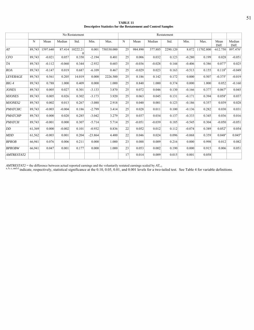
51TABLE 11

Descriptive Statistics for the Restatement and Control Samples

No Restatement Restatement

N Mean Median Std. Min. Max. N Mean Median Std. Min. Max. Mean Diff.

Median Diff.

AT 89,743 1597.640 87.414 10222.210

0.001 750330.000 25 984.890 377.885 2290.120 8.072 11702.800 -612.750 897.476c

CFO 89,743 -0.021 0.057 0.350 -2.194 0.481 25 0.006 0.032 0.123 -0.280 0.199 0.028 -0.051

TA 89,743 -0.112 -0.060 0.344 -2.932 0.603 25 -0.036 -0.028 0.144 -0.406 0.386 0.077a 0.025

ROA 89,743 -0.147 0.019 0.687 -6.109 0.467 25 -0.029 0.023 0.163 -0.513 0.155 0.118b -0.049

LEVERAGE 89,743 0.561 0.205 14.019 0.000 2226.500 25 0.186 0.142 0.172 0.000 0.507 -0.375c -0.019

BIG 4 89,743 0.788 1.000 0.409 0.000 1.000 25 0.840 1.000 0.374 0.000 1.000 0.052 -0.160

JONES 89,743 0.005 0.027 0.301 -3.133 3.870 25 0.072 0.046 0.130 -0.166 0.377 0.067a 0.045

MJONES 89,743 0.005 0.026 0.302 -3.173 3.920 25 0.063 0.045 0.131 -0.171 0.394 0.058a 0.037

MJONES2 89,743 0.002 0.013 0.267 -3.088 2.918 25 0.040 0.001 0.123 -0.186 0.357 0.039 0.028

PMATCHC 89,743 -0.003 -0.004 0.186 -2.799 3.414 25 0.028 0.011 0.100 -0.136 0.282 0.030 0.031

PMATCHP 89,743 0.000 0.020 0.285 -3.042 3.279 25 0.037 0.034 0.137 -0.333 0.345 0.036 0.016

PMATCH 89,743 -0.001 0.000 0.307 -5.714 5.714 25 -0.051 -0.039 0.185 -0.545 0.304 -0.050 -0.051

DD 61,369 0.000 -0.002 0.101 -0.932 0.836 22 0.052 0.012 0.112 -0.074 0.389 0.052a 0.054

MDD 61,562 -0.003 0.001 0.204 -23.864 4.400 22 0.046 0.024 0.096 -0.068 0.359 0.048a 0.045a

BPROB 66,941 0.076 0.006 0.211 0.000 1.000 23 0.088 0.009 0.216 0.000 0.998 0.012 0.082

BPROBW 66,941 0.047 0.001 0.177 0.000 1.000 23 0.053 0.002 0.190 0.000 0.915 0.006 0.051

AMTRESTAT2 17 0.014 0.009 0.015 0.001 0.058

AMTRESTAT2 = the difference between actual reported earnings and the voluntarily restated earnings scaled by ATt-1; a, b, c, and d indicate, respectively, statistical significance at the 0.10, 0.05, 0.01, and 0.001 levels for a two-tailed test. See Table 4 for variable definitions.

52TABLE 12

Logistic Regressions of RESTATE on Measures of Discretionary Accruals

A B C D E F G H I J K Intercept -8.045d -8.153d -8.099d -8.063d -8.099d -8.012d -8.082d -7.780d -7.649d -7.752d -7.748d

AT 0.000 0.000 0.000 0.000 0.000 0.000 0.000 0.000 0.000 0.000 0.000 CFO -0.020 -0.328 -0.598 -0.799 -0.052 -1.162 -1.362a 0.067 -0.895 -1.209 -1.219 ROA 0.172 0.525 0.768 0.963 0.611 1.319 1.403a 0.258 1.143 0.919 0.925 LEVERAGE -1.168 -1.145 -1.168 -1.186 -1.193 -1.207 -1.149 -1.224 -1.310 -1.539 -1.541 BIG 4 0.269 0.295 0.281 0.273 0.268 0.266 0.289 0.097 0.097 0.197 0.196 TA 1.136 JONES 0.777 MJONES 0.338 MJONES2 0.006 PMATCHC 1.313 PMATCHP -0.671 PMATCH -1.293a DD 3.757b MDD 1.424b BPROB 0.087 BPROBW 0.079 Number of restating obs. 25 25 25 25 25 25 25 22 22 23 23 Number of control obs. 89,743 89,743 89,743 89,743 89,743 89,743 89,743 61,369 61,562 66,941 66,941 χ2 4.422 4.469 4.212 4.160 4.614 4.354 6.645 7.691 6.005 4.273 4.270 pseudo R2 0.010 0.010 0.009 0.009 0.010 0.010 0.015 0.020 0.015 0.010 0.010 Odds ratio for DACC 3.114 2.175 1.402 1.006 3.718 0.511 0.274 42.829 4.155 1.091 1.082

a, b, c, and d indicate, respectively, statistical significance at the 0.10, 0.05, 0.01, and 0.001 levels for a two-tailed test. See Table 4 for variable definitions.

53TABLE 13

Logistic Regressions of RESTATE on Measures of Discretionary Accruals After Controlling for Total Accruals A B C D E F G H I J K Intercept -8.045d -8.117d -8.033d -7.999d -8.097d -7.887d -8.033d -7.782d -7.643 -7.737 -7.735 AT 0.000 0.000 0.000 0.000 0.000 0.000 0.000 0.000 0.000 0.000 0.000 CFO -0.020 -0.010 -0.023 -0.069 -0.030 -0.124 -0.252 -0.122 -0.004 -0.447 -0.448 ROA 0.172 0.202 0.169 0.137 0.573 0.163 0.204 0.445 0.240 0.155 0.156 LEVERAGE -1.168 -1.144 -1.172 -1.181 -1.192 -1.207 -1.103 -1.225 -1.306 -1.523 -1.524 BIG 4 0.269 0.286 0.267 0.261 0.268 0.247 0.271 0.098 0.095 0.195 0.195 TA 1.136 0.651 1.222 1.562 0.076 2.559 2.078 -0.208 1.020 1.070 1.075 JONES 0.562 MJONES -0.101 MJONES2 -0.518 PMATCHC 1.260 PMATCHP -1.810 PMATCH -1.545b DD 3.779b MDD 1.414b BPROB 0.058 BPROBW 0.067 Number of restating obs. 25 25 25 25 25 25 25 22 22 23 23 Number of control obs. 89,743 89,743 89,743 89,743 89,743 89,743 89,743 61,369 61,562 66,941 66,941 χ2 4.422 4.539 4.425 4.511 4.614 5.247 7.849 7.695 6.065 4.475 4.475 pseudo R2 0.010 0.010 0.010 0.010 0.010 0.012 0.017 0.020 0.016 0.011 0.011 Odds ratio for DACC 1.755 0.904 0.596 3.524 0.164 0.213 43.755 4.111 1.060 1.070

a, b, c, and d indicate, respectively, statistical significance at the 0.10, 0.05, 0.01, and 0.001 levels for a two-tailed test. See Table 4 for variable definitions.

54TABLE 14

Regressions of AMTRESTAT2 on Measures of Discretionary Accruals for a Common Sample

A B C D E F G H I J K Intercept 0.041b 0.041a 0.035 0.053a 0.052b 0.039b 0.016b 0.035a 0.038b 0.058b 0.055c

ASSETS 0.000 0.000 0.000 0.000 0.000 0.000 0.000 0.000 0.000 0.000 0.000 CFO 0.039 0.002 0.016 -0.069 -0.172 -0.004 0.070 0.039 0.052 -0.028 -0.027 ROA 0.039 0.038 0.004 0.074 0.108 -0.011 0.037 0.036 0.022 0.002 0.010 LEVERAGE -0.024 -0.024 -0.017 -0.017 -0.008 -0.011 0.029 -0.023 -0.011 -0.012 -0.011 BIG4 -0.025 -0.025 -0.025 -0.031 -0.026 -0.030 0.020 -0.023 -0.031 -0.040a -0.039a

TA -0.003 JONES -0.002 MJONES 0.049 MJONES2 -0.087 PMATCHC -0.204 PMATCHP 0.066 PMATCH 0.039 DD 0.061 MDD 0.093 BPROB -0.050 BPROBW -0.050 N 14 14 14 14 14 14 14 14 14 14 14 F-Value 1.30 0.95 1.12 1.57 2.55 1.36 0.95 1.04 1.32 1.78 1.92 Adjusted R2 0.104 -0.024 0.052 0.208 0.418 0.143 -0.021 0.020 0.130 0.264 0.299

a, b, c, and d indicate, respectively, statistical significance at the 0.10, 0.05, 0.01, and 0.001 levels for a two-tailed test. See Table 4 for variable definitions.