1  

SESHD Working Paper #2017-39

Do Older Americans Have More Income Than We Think?

Adam Bee (U.S. Census Bureau)

Joshua Mitchell (U.S. Census Bureau)

July 2017

Abstract

The Current Population Survey Annual Social and Economic Supplement (CPS ASEC) is the source of the nation’s official household income and poverty statistics. In 2012, the CPS ASEC showed that median household income was $33,800 for householders aged 65 and over and the poverty rate was 9.1 percent for persons aged 65 and over. When we instead use an extensive array of administrative income records linked to the same CPS ASEC sample, we find that median household income was $44,400 (30 percent higher) and the poverty rate was just 6.9 percent. We demonstrate that large differences between survey and administrative record estimates are present within most demographic subgroups and are not easily explained by survey design features or processes such as imputation. Further, we show that the discrepancy is mainly attributable to underreporting of retirement income from defined benefit pensions and retirement account withdrawals. Using archived survey and administrative record data, we extend our analysis back to 1990 and provide evidence of underreporting from an earlier period. We also document a growing divergence over time between the two measures of median income which is in turn driven by the growth in retirement income underreporting. Turning to synthetic cohort analysis, we show that in recent years, most households do not experience substantial declines in total incomes upon retirement or any increases in poverty rates. Our results have important implications for assessing the relative value of different sources of income available to older Americans, including income from the nation’s largest retirement program, Social Security. We caution, however, that our findings apply to the population aged 65 and over in 2012 and cannot easily be extrapolated to future retirees. ______________________________________________________________________ 

The views expressed herein are those of the authors and do not necessarily reflect the views of the US Census Bureau. All results have been formally reviewed to ensure that no confidential Census Bureau data have been disclosed. We thank Jonathan Rothbaum, Trudi Renwick, Sonya Porter, and Mark Leach for their support and reviews; Lori Reeder, Gary Benedetto, Gloria Duval, John Eltinge, and Julia Manzella for their reviews, seminar participants at SSA, IRS, GAO, the NBER Women Working Longer workshop, the Federal Reserve Board of Governors, and CBO for their insightful comments; Patricia Ruggles, Courtney Coile, and John Sabelhaus for their discussions; Jessica Holland, Kevin Pierce, Dan Feenberg, Dylan Rassier, Amy O’Hara, and Victoria Bryant.

 

2  

I. Introduction

Are Americans adequately prepared for retirement? Using a variety of methods and assumptions, researchers have arrived at starkly different answers to this important question. Common to nearly all approaches, however, is a reliance on household survey data to measure the economic resources available to older Americans. Yet, it has long been recognized that income aggregates derived from popular household surveys fall short of comparable administrative record totals.1 For older Americans in particular, analysts have raised concerns that survey-based income aggregates from employer-sponsored retirement plans and IRAs appear to be too small.2

By itself, however, evidence of aggregate income underreporting cannot address a key distributional question: Does income underreporting only affect the measured economic status of the wealthiest households, or does it broadly alter our understanding of the well-being of older Americans? This question has remained unanswered to date because it requires validation of survey income responses on a person-by-person basis.

In this paper, we overcome this obstacle and develop new, nationally representative estimates of income and poverty for the population aged 65 and over. We do this by linking survey data collected by the U.S. Census Bureau with an extensive array of administrative income records from the Social Security Administration (SSA) and the Internal Revenue Service (IRS) spanning nearly a quarter century.

Our starting point is the Census Bureau’s Current Population Survey Annual Social and Economic Supplement (CPS ASEC), the source of the nation’s official income and poverty statistics. We focus on comparing five types of income available in both the CPS ASEC and the administrative records: earnings, Social Security benefits, Supplemental Security Income (SSI), interest and dividends, and retirement income. By retirement income, we mean all amounts received from defined benefit pension plans including survivor and disability payments (excluding Social Security) as well as all employer and IRA defined contribution distributions that permanently leave tax-preferred accounts.3

Replacing survey income responses with administrative record values leads to several striking findings. First, relative to the 2012 number derived from the CPS ASEC alone, the median income for householders aged 65 and over is 30 percent higher in the linked sample (rising from $33,800 to $44,400). Second, the poverty rate for persons aged 65 and over is 2.1 percentage points lower in the linked sample (falling from 9.0 to 6.9 percent). Third, across most of the income distribution, we find that retirement income underreporting is mainly responsible for the overall income discrepancy, while self-reported earned income and Social Security                                                             1 For example, Rothbaum (2015) compares Census survey income aggregates to the National Income and Product Accounts which in turn derive many of its numbers from administrative records. 2 Schieber (1995) provides an early example of this argument. Woods (1996) critiques his analysis. 3 We discuss alternative income concepts in Section III.

 

3  

benefits correspond well with administrative records. Further, the underreporting of retirement income occurs mostly at the extensive margin—that is, people who actually receive retirement income fail to report any of it in the survey 46 percent of the time. In contrast, when reported, retirement income amounts in the CPS ASEC match administrative record amounts fairly well.

We next explore potential reasons why the two measures of retirement income diverge. Demographic characteristics are only weakly related to false negative reports. Additionally, most survey design features such as imputation cannot explain the gap. The most powerful predictors of underreporting are the characteristics of the actual retirement income received. Those with larger and more stable amounts of administrative record retirement income are more likely to report receipt in the survey. Consistent with concerns raised in the literature, distributions from IRAs are rarely reported. Nonetheless, we show that even those with considerable amounts of employer-sponsored retirement income still have high false negative rates. Even those who receive distributions from traditional government defined benefit plans still frequently fail to report them. Thus, while the previous literature has related aggregate discrepancies to the transition to defined contribution systems, it has largely ignored the possibility that defined benefit income is also underreported.

Using archived administrative record data, we extend our linked sample analysis of income and poverty back nearly a quarter of a century. We find that there was a smaller but still substantial median income discrepancy of 20 percent in 1990 such that the survey shows median incomes grew only 18 percent between 1990 and 2012, while the administrative records show growth of 29 percent.4 Paralleling the rising median income gap is a rise in retirement income false negatives. Remarkably, the survey shows no evidence of any rise in retirement income receipt during this period, with an estimated rate of receipt of 40 percent in 1990 and 36 percent in 2012. In contrast, the administrative records show over this same period that the rate of receipt rises from 45 percent to 61 percent. Meanwhile, poverty rates are lower in the administrative records in all years examined, although the trend in poverty rates is largely unaffected.

Our new income measures change the relative importance of different sources of income available to the aged. In particular, we show that throughout much of the income distribution, Social Security is a smaller share of total income in large part due to the higher measures of retirement income. We also show at the bottom of the distribution that survey respondents frequently confuse Social Security with SSI such that SSI plays a larger role among the low-income aged population than the survey suggests. In light of this, we reassess commonly cited statistics on the share of beneficiaries depending on Social Security income and the number of people lifted out of poverty by Social Security. In particular, the share of beneficiaries that

                                                            4 We calculate variances for 1990 by multiplying the CPS 1990 margin of error by the same ratio of the admininstrative 2012 margin of error to the CPS 2012 margin of error, since neither generalized variance functions nor replicate weights are available.

 

4  

depend on Social Security for at least 90 percent of their income falls by half, and the number of people lifted out of poverty by Social Security falls by one-third.

Our distributional analysis does not discount, however, the relative importance of total annuitized income. We develop a novel methodology to identify types of administrative record retirement income and find that defined benefit income is still the predominant source of retirement income for most of the aged in 2012.

Lastly, we conduct a synthetic cohort analysis that compares incomes and poverty rates during an 11-year window surrounding the claiming of Social Security benefits. The survey measures show overall income drops that are twice as large as the administrative records as well as substantially larger increases in the proportion of claimants living under 200 and 300 percent of the poverty threshold. Overall, when using the administrative records, we find income declines that are gradual and predate retirement as well as no evidence of an increase in poverty rates. Further, income five years after claiming Social Security remains high relative to measures of career-average earnings.

We argue these results challenge the “retirement consumption puzzle,” the finding in many household surveys that consumption, particularly food consumption, appears to decline sharply at retirement. This is considered a puzzle because it implies that many households are myopic and fail to save adequately for retirement, which contradicts the predictions of the standard lifecycle model. When using the administrative records, however, we do not find large, abrupt declines in income or increases in poverty upon retirement. Thus, we argue that the premise of the puzzle is not correct—retirement does not appear to be a fruitful setting to examine consumption responses to a large, predictable decline in income.

While our work yields many new and surprising findings, we are certainly not the first to call attention to the measurement of retirement income in the CPS ASEC (Anguelov et al., 2012; Czajka and Denmead, 2012; Gustman et al., 2014; Iams and Purcell, 2013; Munnell and Chen, 2014; Sabelhaus and Schrass, 2009). The CPS ASEC underwent a redesign in survey year 2014. This was done in part to improve the collection of retirement incomes in an environment where retirees will increasingly rely on irregular withdrawals from defined contribution retirement accounts. Evaluations of the redesign found modest improvements in median incomes and no evidence of any change in poverty for the aged (Semega and Welniak, 2015; Mitchell and Renwick, 2015). In this paper, we only reevaluate the traditional CPS ASEC, but we hope to examine the redesigned version in future work as more recent years of administrative record data become available.

We must also acknowledge several important caveats to our findings. First and foremost, our revised income and poverty measures apply to the aged population through 2012 and cannot easily be extrapolated to future retirees. There are many demographic, labor market, and retirement policy changes that future cohorts will face. For example, future cohorts will have

 

5  

access primarily to defined contribution plans. How they will fare in retirement remains an open question. Second, even among recent retirees, incomes cannot capture all relevant aspects of material well-being. If Americans are entering retirement with rising debt levels that they must service, then higher incomes may not translate into higher consumption (Lusardi and Mitchell, 2017; Butrica and Karamcheva, 2013). On the other hand, our study reevaluates only five sources of income. To the extent other sources of income are also underreported among the aged, total incomes could be even higher than what we find.

The rest of this paper proceeds as follows. Section II reviews the relevant literature. Section III discusses alternative income concepts. Section IV describes the survey and administrative record data. Section V presents results. Section VI concludes.

II. Review of Literature

Our work builds on previous efforts to measure the economic well-being of the aged. Studies that compare income and consumption-based measures of total resources and poverty are particularly relevant. Cutler and Katz (1991a, b), Hurd and Rohwedder (2006), and Meyer and Sullivan (2010, 2012) argue that consumption-bases measures are attractive from both a conceptual and practical standpoint. Consumption may be a better proxy for long-run living standards if individuals can access savings to smooth over temporal fluctuations. A consumption-based poverty measure may also have practical value if survey respondents have special difficulty reporting certain types of income. This may be particularly relevant for the aged, who are increasingly dependent upon a complex array of retirement income resources. These studies suggest considerably more economic progress for the aged when using survey-based measures of consumption rather than income. Using linked data, our work provides an explanation for these disparate findings. Consumption-based measures may indeed be more accurate if retirement income is underreported.

Other studies focus on measuring consumption at the onset of retirement. As mentioned, the standard lifecycle model predicts that households should want to avoid sharp drops in consumption in response to anticipated changes in income. Yet many prominent studies, such as Bernheim et al. (2001) and Banks et al. (1998), have found that consumption, including food consumption, does fall considerably at retirement, implying that households are myopic.

More recent studies have questioned the retirement consumption puzzle. Hurst (2008) argues that evidence of a consumption decline is limited to two categories: work-related expenses, and food expenditures. With respect to food, expenditures need not be the same as consumption. Aguiar and Hurst (2005, 2007) show that retiring households increase time spent on food preparation and time spent shopping for bargains and substitute away from spending on meals outside the home. The result is a decline in food spending but not in food consumption. Households that do experience large consumption declines at retirement tend to be those that

 

6  

experience permanent health shocks, as shown in Hurd and Rohwedder (2013). This behavior is consistent with the standard lifecycle model.

What happens to incomes at the onset of retirement is less studied, however. In this paper and in our related work on women’s retirement behavior (Bee and Mitchell, 2016) we do not find strong evidence of large, abrupt declines in incomes at retirement. Similarly, Brady et al. (2017) find, using a sample of tax filers, that most households are able to maintain their income available for spending three years after retirement. Together, these papers call into question the premise of the retirement consumption puzzle—that there are predictable declines in incomes at retirement.

Another issue is whether households can maintain their standard of living many years into retirement. One way to address this question is to examine the trajectory of wealth during retirement years. Love et al. (2008) find evidence that wealth declines more slowly than remaining life expectancy. De Nardi et al. (2010) attribute the slow decline of wealth to precautionary savings for rising out-of-pocket medical expenses. Poterba et al. (2015) demonstrate that wealth is remarkably persistent in retirement. Consistent with our findings, a slow decline in retirement wealth may be feasible if retirees in fact have higher incomes than previously thought.

Our work also provides useful context for studies that forecast the well-being of future retirees (Skinner, 2007). More optimistic studies find favorable comparisons between observed savings behavior during working years and predictions of optimal behavior based on augmented lifecycle models or other established benchmarks (Butrica et al., 2012; Devlin-Foltz et al., 2016; Engen et al., 1999; Hubbard et al., 1995; Scholz et al., 2006). On the other hand, some studies argue that a majority households face saving shortfalls and will be unable to maintain their standard of living in retirement (Bernheim et al., 2000; Munnell et al., 2014). Our results suggest that future work should examine the sensitivity of these survey-based predictions to other measures of resources available in administrative records.5

Lastly, our work relates to the large literature examining survey measurement error. Besides our own exploratory work in Bee (2013) and our examination of women’s retirement in Bee and Mitchell (2016), there have not been previous microdata studies that validate retirement income. Survey methodologists have found indirect evidence, however, that asking about retirement account withdrawals immediately after asking about account balances improves survey retirement income reporting in the Survey of Consumer Finances and the Health and Retirement Study (Argento et al., 2015; Bosworth and Burke, 2012).

Others have examined survey responses to retirement plan participation questions during working years. Early work by Mitchell (1988) with the SCF and a comprehensive survey by Gustman et al. (2010) using the HRS find that many participants are unaware of key plan

                                                            5 Some of these studies do make use of administrative-record earnings histories.

 

7  

features and often confuse defined benefit with defined contribution plans. Recent work using household surveys linked to earnings records reveals that self-reports of defined contribution participation are biased downward (Dushi and Honig, 2015; Dushi and Iams 2010). It is perhaps not surprising that if survey participants have difficulty reporting retirement plan information during working years, they continue to have difficulty after they retire.

III. Income Concepts

There are many different perspectives on what should be counted as income. The classic Haig-Simons income is defined as the maximum amount that can consumed without lowering net worth. In this framework, income in retirement plans should be counted as it accrues. Most household surveys do not attempt this. The CPS ASEC was designed to collect money income which is defined as “income received on a regular basis (exclusive of certain money receipts such as capital gains) before payments for personal income taxes, Social Security, union dues, Medicare deductions, etc.” 6,7 While traditional defined benefit/annuity income clearly satisfies the money income criteria and should be captured by the survey, the private sector transition to defined contribution systems poses a conceptual challenge for the CPS ASEC. Retired individuals may opt to make withdrawals from their defined contribution accounts on an as-needed rather than regular basis. These withdrawals could be considered dissaving rather than income. Issues such as the proper treatment of rollovers (moving money from one tax-preferred account to another) and other lump-sum distributions further complicate matters. Yet another concern is that some withdrawals from retirement accounts reflect past employee contributions that already would been counted as wage income. Prior to the redesign, the CPS ASEC only sought to count payments from IRAs and other defined contribution accounts to the extent they were received regularly.

Other federal agencies rely on different income concepts. For example, the IRS excludes from income the contributions made to (non-Roth) defined contribution accounts as well as the interest, dividends, and capital gains accrued within those accounts. At the time money is withdrawn, it is included in income and subject to taxation. The Bureau of Economic Analysis (BEA) uses yet another set of standards for national income accounting purposes. International guidelines from the 2008 System of National Accounts state that retirement plans should be treated as redistributions so that measures of disposable income reflect retirement benefit payments rather than accrual-based income. However, the U.S. does not follow international guidelines and instead counts contributions as well as interest and dividends (but not capital gains) when earned in its measure of disposable income. McCully (2014) and Lusardi et al. (2001) discuss advantages of adhering to the international guidelines.

                                                            6 Ruser et al. (2004) compare Haig-Simons, personal, and money income concepts. 7 https://www.census.gov/topics/income-poverty/income/about.html

 

8  

Some researchers have sought a middle ground between income and consumption. As discussed earlier, consumption may serve as a better proxy for well-being, particularly for the aged. Using survey data, Short and Skog (2014) explore how including retirement account withdrawals net of contributions as resources available to spend on basic needs would change the Supplemental Poverty Measure for the population aged 65 and over. Brady et al. (2017) develops the concept of “spendable income” which is a measure of after-tax income that also incorporates retirement account withdrawals net of contributions.

In this paper, we count all gross distributions that permanently leave tax-preferred retirement plans as income, regardless of whether they are taxable in that year. This includes payments received from defined benefit plans, as well as employer defined contribution and IRA withdrawals (both traditional and Roth). To avoid double-counting, we exclude distributions such as direct rollovers and conversions which simply move money across different tax-preferred accounts. Our definition is consistent with the goals of SSA researchers Anguelov et al. (2012) who argue that household surveys including the (traditional) CPS ASEC “need to revise their measures of retirement income to account for periodic (irregular) distributions from DC plans and IRAs.” Beginning with survey year 2014, the redesigned CPS ASEC now includes irregular distributions in income. Our measure is also consistent with the family income numbers released in the Federal Reserve Bulletin which incorporate both pensions and withdrawals from retirement accounts.8  Lastly, the decision to count withdrawals as income is also a practical one, given the administrative record data that have been made available to us. We describe these data next.

IV. Data

We bring together several survey and administrative record data sources to reassess incomes of older Americans. We describe each of them below.

The primary purpose of the CPS is to measure the monthly unemployment rate for the civilian non-institutionalized population. Between February and April, the CPS ASEC collects detailed information on amounts and sources of incomes received in the previous calendar year for approximately 75,000 households. These data have been used to produce annual income and poverty statistics since 1959. The first part of our analysis focuses exclusively on reference year 2012. We later extend our analysis to cover reference years 1990, 1995, and 1998-2012.

While incomes are collected for each household member aged 15 and over, we focus on total pre-tax household income and classify households by the demographic characteristics of the householder as in DeNavas-Walt et al. (2013). Unlike the annual report, we restrict our attention to householders aged 65 and over. When measuring poverty, the resource unit is either a family or an unrelated individual rather than the household. A family is defined as two or more persons

                                                            8 See “Changes in U.S. Family Finances from 2010 to 2013: Evidence from the Survey of Consumer Finances” https://www.federalreserve.gov/pubs/bulletin/2014/pdf/scf14.pdf

 

9  

related by blood, marriage, or adoption. A person is classified as in poverty if total pre-tax family (or unrelated individual) income is below the relevant poverty threshold which varies based on family size and composition. Similar to income, we examine the poverty status of persons aged 65 and over.9

Of particular interest are the CPS ASEC questions related to retirement income. There are several points during the interview where respondents might report such income. The main CPS ASEC question is:

“During 2012 did (you/ anyone in this household) receive any pension or retirement income from a previous employer or union, or any other type of retirement income (other than Social Security or VA benefits) ?

If the respondent indicates someone in the household received such income, follow-up questions ask who in the household received the income, the amounts received, and the particular sources of this income. There are also parallel questions for disability and survivor income (also apart from VA Benefits and Social Security) which are included in our definition of retirement income. We also choose to include VA pension, survivor, and disability payments asked earlier in the interview because we have reason to believe some respondents may misclassify their military pensions as VA benefits.10 Lastly, the CPS ASEC asks a final question about any other income not already mentioned. If respondents indicate they have other income either from pensions or annuities, we include this in our measure of retirement income.

The CPS ASEC is linked to several administrative record sources supplied by the Social Security Administration.11 These include data on annual earnings from both wage and salary jobs (IRS form W-2) and self-employment (IRS 1040 schedule SE), total OASDI benefits received (including any deductions for Medicare premiums), and total SSI benefits (including any state supplements). Up through 1990, the SSA earnings records also include information from IRS form W-2P “Statements for Recipients of Annuities, Pensions, Retired Pay, or IRA payments”

                                                            9 In supplementary analysis, we make use of two additional Census surveys which we also link to select administrative records: the Survey of Income and Program Participation (SIPP) and the American Community Survey (ACS). We discuss linkages to the SIPP in Bee and Mitchell (2016) and linkages to the ACS in Bee et al. (2016).

10 This will bias our survey measure of retirement income upward relative to the administrative records because VA Benefits are not taxable and do not show up in the available administrative records. 11 Persons in the CPS ASEC are linked to administrative records via the Personal Identification Key (PIK), a scrambled SSN. In recent years, the PVS process is used to assign a PIK to approximately 90% of people aged 65 and over. Details of the PVS process are contained in Wagner and Layne (2014). We reweight the PIK subsample to be representative of the full sample. Specifically, we run a logistic regression to model the likelihood of being assigned a PIK as a function of survey demographic and income characteristics. We then multiply the CPS ASEC survey weight by the inverse of the estimated propensity score. Individuals with a PIK who fail to match to a given administrative income source (besides Form 1040) are assumed to not have any income from that source. We are unable to link persons not assigned a PIK to administrative records. For these persons, we continue to use their survey income values. Incomes of persons without a PIK are incorporated into the total family and household incomes of persons who are assigned a PIK.

 

10  

which allow us to measure periodic payments of retirement income during an early time period.12 Lastly, SSA also supplies the Census Bureau with the Numident file which contains date of birth and date of death information used in parts of our analysis.

We also link the CPS ASEC to two types of universe records obtained from the IRS. The first is the information return form 1099-R “Distributions From Pensions, Annuities, Retirement or Profit-Sharing Plans, IRAs, Insurance Contracts, etc.” Available to us from the 1099-R are the gross distributions from employer-sponsored plans (both defined benefit and defined contribution) as well as IRA withdrawals which we combine to measure total retirement income from 1995 onward.13 Besides the IRA/employer-sponsored distinction, we do not receive any additional information about the types of distributions received.14 Importantly, however, the IRS excludes certain kinds of distributions from our extracts which we would not wish to consider income. The main types of excluded distributions are direct rollovers, Section 1035 exchanges, and Roth conversions. Together with the form W-2P for early years (which never included rollovers), the 1099-R provides administrative record measures of retirement income spanning over three decades.

The second type of record obtained from IRS is the form 1040 filed by taxpayers for tax years 1989, 1995, and 1998-2012. Total dividend income as well as taxable and tax-exempt interest are available to us from the 1040. For joint filers, we assume an even split of dividend and interest income among the primary and secondary filer, and we assume zero asset income for dependents. Not everyone files a 1040 each year, so for non-filers we simply use the CPS ASEC values for interest and dividends.

Appendix Table 1 shows the five types of income in the CPS ASEC that we validate, the survey variable definitions, and the corresponding administrative record sources. Outside these five types of income, we continue to use the CPS ASEC values in constructing total incomes.15 After creating new measures of total income for each person, we aggregate up to the household level to recalculate standard median income statistics and to the family level to reevaluate poverty status.

                                                            12 As far as we are aware, we are the first to take advantage of this high-quality administrative record source of historical retirement income data. See Bee and Mitchell (2016) for a comparison of women’s retirement incomes extending back to the 1980s using Form W-2P data. 13 An advantage of measuring retirement distributions from the information return is that we capture this income regardless of whether someone files a 1040 in that particular year. Taxpayers who are required to file are instructed to transfer the applicable amounts from the 1099-R to lines 15 and 16 of the Form 1040. Lines 15a and 16a are meant to capture gross amounts while 15b and 16b capture taxable amounts. Our 1099-R extracts include some amounts that are not taxable such as Roth distributions. This is consistent with our aim of measuring retirement income once when it permanently leaves the tax-preferred system. 14 The IRA category also includes SEP and SIMPLE type plans. 15 Other types of income collected by the CPS ASEC include unemployment compensation, workers’ compensation, public assistance, rents/royalties/estates/trusts, educational assistance, alimony, child support and financial assistance from outside the household. Within the survey, the five sources we validate account for 97 percent of aggregate total income among persons aged 65 and over.

 

11  

V. Results

V.1. Analysis of Aggregates

We begin with a comparison of 2012 aggregate income amounts. Table 1 computes three sets of aggregates for two age groups, persons aged 18 to 64 and persons aged 65 and over. The first set of aggregates, shown in column 1, is derived from the “Full CPS Sample,” and totals five types of income (earnings, Social Security, SSI, interest & dividends, and retirement income) from the complete 2013 CPS ASEC sample. The second set of aggregates, shown in column 2, is calculated from the “CPS PIK Sample”, the subset of persons in the Full CPS Sample who are assigned a PIK. The CPS PIK Sample is reweighted to represent the Full CPS Sample and also uses survey responses to calculate income aggregates. The third set of aggregates is labeled the “Linked CPS-Admin Sample” and is shown in column 3. This is the same set of persons as the CPS PIK Sample but uses administrative record values rather than survey responses to calculate aggregates.

Column 4 makes the direct comparison between survey and administrative aggregates by expressing the CPS total (from column 2) as a share of the administrative record total (from column 3). For both age groups, CPS earned income tracks the administrative record measure very closely, accounting for approximately 100 percent of the target amount for those aged 18 to 64 and 98 percent of the target amount for those aged 65 and over. Social Security benefits are also reported relatively well, particularly for the aged. The CPS captures 83 percent of the target amount for those aged 18 to 64 and 96 percent of the target amount for those aged 65 and over.16 CPS reporting of SSI benefits is more complex. Persons aged 18 to 64 appear to overreport SSI, while those aged 65 and over only report 73 percent of the target amount.17 However, SSI misreporting is modest in the aggregate because SSI benefits account for only a small share of total income for both age groups.18 In contrast, the underreporting of asset income is evident for both age groups and is important in the aggregate for persons aged 65 and over. Specifically, CPS interest and dividends account for only 77 and 63 percent of their respective targets. For persons aged 65 and over, interest and dividends represent 11 percent of their total incomes in the administrative records.19

                                                            16 When using administrative record rather than survey values, Social Security’s share of aggregate income falls from 39 percent to 31 percent for persons aged 65 and over. We discuss changes in the relative importance of Social Security in Section V.10. 17 In the CPS, adults are also requested to report SSI benefits received on behalf of any children under age 15. In order to compare to the administrative records, we subtract child benefits from the survey aggregates to restrict to SSI benefits received by adults. There appears, however, to be relatively few respondents who indicate any child SSI receipt. This raises the possibility that some of the reported adult SSI benefits are misclassified and the survey SSI aggregate amount for persons aged 18 to 64 is inflated. If we instead included administrative record amounts of SSI received by children aged 0 to 14 together with their parents, this would result in an additional 7 billion dollars of SSI benefits among persons aged 18 to 64 and bring the two data sources into closer alignment. 18 “Total income” in Table 1 refers to the combined income from the five sources where administrative records are available. 19 Comparions beyond those explicitly stated are not tested for statistical significance.

 

12  

Most striking are the retirement income comparisons. The CPS accounts for only 45 percent of the target for persons aged 18 to 64 and 48 percent of the target for persons aged 65 and over. Naturally, retirement income underreporting is more consequential for the measurement of older Americans’ incomes. In the administrative records, retirement income accounts for only 5 percent of total income for persons aged 18 to 64 but 34 percent of total income for persons aged 65 and over. For this reason, overall income underreporting differs markedly by age group. Because earned income is the dominant income source for persons 18 to 64 and is reported very well, the CPS still captures 96 percent of total income for this age group. In contrast, the CPS captures only 76 percent of total income for persons aged 65 and over. For the remainder of our analysis, we therefore focus on the consequences of income underreporting among the older population.

Our aggregate comparisons represent an improvement over previous studies because we are able to examine underreporting for the same set of individuals and report our results separately for the aged and non-aged populations. However, the main advantage of the linked microdata is that we can move beyond aggregates and examine the full distributional implications of income underreporting. We therefore turn to the analysis of median incomes.

V.2. Analysis of Median Incomes

Table 2 compares survey and administrative record estimates of median household income. Consistent with the annual income and poverty report (e.g., DeNavas-Walt et al., 2013), households are classified by the demographic characteristics of the CPS householder. Results are again shown for the Full CPS Sample, the CPS PIK Sample, and the Linked CPS-Admin Sample. Column 4 computes the percentage difference between the administrative record and survey values. Among all householders aged 65 and over, median incomes are 30 percent higher in the administrative records ($44,400 versus $34,000). As the table indicates, economically meaningful and statistically significant median differences are found among a wide variety of family, race/ethnicity, age, nativity, disability, region, residence, educational attainment, housing tenure, and veteran status subgroups. For example, the median difference is 21 percent for those aged 65 to 74, 37 percent for those aged 75 to 84, and 33 percent for those 85 and over. Income differences are also not strongly related to proxies for socioeconomic status such as educational attainment. Householders of all educational attainment levels have large median income differences. Overall, our results demonstrate that correcting for income underreporting meaningfully changes our assessment of the material well-being of the typical aged household.20

V.3. Analysis of Poverty Rates

Table 3 examines survey- and administrative record-based poverty rates for persons aged 65 and over. Among all aged persons with a PIK, the poverty rate falls from 9.0 percent in the

                                                            20 In Appendix Table 2, we run separate median regressions for survey and administrative record income that include all demographic variables listed in Table 2 as covariates.

 

13  

survey to 6.9 percent in the linked sample. Poverty rates also fall when we classify persons by family status, race/ethnicity, gender, age, region, residence, disability, educational attainment, housing tenure, and veteran status. The new poverty estimates are not only lower, but in some cases, they alter our understanding of the relative well-being of the various demographic subgroups. For example, the survey suggests that poverty rises sharply by age—7.9 percent for those aged 65 to 74, 9.8 percent for those aged 75 to 84, and 12.1 percent for those aged 85 and over. In contrast, the administrative records show a much flatter pattern—6.7 percent, 7.0 percent, and 7.6 percent, respectively. Although this comparison is cross-sectional, it is consistent with a greater ability of households to maintain their standard of living as they age.

Another illustrative comparison is housing tenure, a useful survey-based proxy for wealth. The survey shows considerably higher poverty rates for those who own a home without a mortgage than for those who have a mortgage, 7.3 percent versus 4.6 percent. The administrative records indicate a much smaller gap, 4.4 percent versus 3.1 percent. Aged renters, on the other hand, have a much higher survey-based poverty rate of 21.3 percent, and there is no evidence of a decline when using the administrative records to measure income.

Other common poverty group comparisons are only modestly changed when using the administrative records. For example, the survey shows that poverty rates are higher for women than men, 10.8 percent versus 6.7 percent. Using the administrative records, the rates are lower for both sexes but still 8.5 percent for women versus 4.9 percent for men. Overall, the results in Table 3 show that income underreporting meaningfully affects our assessment of poverty among the aged.21

V.4. Accounting for the Overall Income Discrepancy

The results in Tables 2 and 3 incorporate all five administrative record income sources at once. Naturally, this raises the question of which income source is most responsible for our findings. In Table 4, Panel A, we recalculate several iterations of household income percentiles as well as the fraction of people below specified thresholds of the income to poverty ratio. The results are also shown graphically for every percentile in Figure 1. For each iteration, one survey income source is swapped with its administrative record counterpart and then households (for income) and persons (for poverty) are re-ranked based on this new measure of total income. The change is then computed relative to the CPS baseline values. The swapping is cumulative so that by the end of the fifth iteration, all administrative record sources are included in income.22 Column 2 shows the effect of swapping earned income, column 3 shows the effect of swapping earned income and Social Security, and column 4 shows the effects of swapping earned income, Social Security, and SSI. Across these columns, few economically meaningful differences in household income percentiles are found relative to the CPS baseline. Somewhat larger effects are

                                                            21 In Appendix Table 3, we run separate linear probability models for survey and administrative record poverty status that include all demographic variables listed in Table 3 as covariates. 22 Table 4, Panel B repeats this exercise but examines the effect of swapping each income source on its own.

 

14  

found (in proportional terms) when interest and dividends are also swapped in column 5, particularly in the bottom half of the income distribution. As shown in column 6, however, the large overall income differences found can be attributable to replacing survey with administrative record measures of retirement income. This holds across much of the income distribution. For example, swapping the first four income sources results in a 7 percent higher 25th percentile of household income (relative to the CPS baseline 25th percentile), while also swapping retirement income increases this difference sharply to 26 percent. At the 75th percentile, there is only a 1 percent income difference after swapping the first four income sources, but after retirement income is also swapped, the overall income difference jumps to 22 percent.

Retirement income is somewhat less dominant when looking at the change in the measured proportion of persons in poverty. Still, it remains the single most important factor, accounting for 1.2 of the total 2.1 percentage point decline. At higher income to poverty ratios, retirement income’s importance is also apparent, accounting for 6.4 of the 9.8 percentage point reduction in persons with incomes below 200 percent of poverty. Clearly, the underreporting of retirement income is central to understanding the overall income discrepancies found. This holds across broad swaths of the income distribution.

V.5. Understanding Retirement Income Underreporting

In explaining why survey and administrative record measures of retirement income differ so dramatically, it is useful to classify potential types of misreporting. A false negative refers to the absence of survey income when income is in fact present in the administrative records. A false positive refers to the presence of survey income but no income found in the administrative records. Of course, for many individuals, the two data sources are consistent. In such cases, a true negative refers to zero income in both data sources and a true positive refers to positive income in both data sources. When analyzing misreporting, we also distinguish between receipt of any income and the amount of income received, conditional on receipt. Underreporting at the extensive margin is simply a false negative report. Underreporting at the intensive margin refers to a true positive report, but a lower income amount recorded in the survey than in the administrative records.23

                                                            23 There is some ambiguity here. Individuals may in fact receive distributions from multiple retirement plans, each generating its own 1099-R form. (Appendix Table 4 reports the distribution of the number of 1099-Rs received). Survey respondents also have the opportunity to report multiple sources of retirement income. Thus, it is possible for a respondent to accurately report one type of retirement income but neglect to mention a second type of retirement income. In this case, we classify this respondent as a true positive report with underreporting at the intensive margin because the total amount of retirement income reported is lower than the total amount in the administrative records. Alternatively, one could attempt to track the quality of reporting for each separate retirement account, in which case the failure to mention the second account could be considered extensive margin underreporting. Relative to this alternative classification system, we will tend to understate the incidence of underreporting at the extensive margin and overstate the amount of underreporting at the intensive margin.

 

15  

Along these lines, Table 5 decomposes the impact of different types of retirement income misreporting across the household income distribution, across various income to poverty thresholds, and across the person-level retirement income distribution. We begin in column 1 with the CPS baseline values and correct in a cumulative fashion for each type of retirement income misreporting. In column 2, we replace the false positives with zeros which can only lower incomes and raise poverty estimates. In column 3, we replace true positives with administrative record values which corrects for intensive margin misreporting. In column 4, we replace false negatives with administrative record values which raises incomes and lowers poverty estimates. Columns 5 through 7 then calculate the percentage of the total measured income or poverty change that is attributable to each type of correction. Note that the three corrections must sum to 100 percent so while correcting for false positives produces a negative income change, the other two corrections must account for more than 100 percent of the overall positive change. Lastly, column 8 then swaps the remaining four types of survey income for their administrative record counterparts to reinforce that most of the total income change is in fact due to corrections for retirement income misreporting.

Eliminating retirement income false positives somewhat reduces incomes toward the bottom of the income distribution (and raises poverty rates), although the absolute declines are small economically. Replacing true positives also has little impact at the bottom of the income distribution. As incomes rise, intensive margin underreporting becomes more relevant, accounting for 38 percent of the overall income change at the 75th percentile. Across the income distribution, however, it is clear that false negatives are the single largest component of retirement income underreporting.24 They account for 103 percent of the total change at the 25th percentile and 70 percent of the change at the 75th percentile.25

Another way to demonstrate the centrality of the extensive margin is to compare income correlations and rates of receipt across types of income. As shown in Appendix Table 6 the log-log correlation between survey and administrative record retirement income is 0.53, which compares favorably to the correlation for Social Security, 0.56. In other words, retirement income intensive margin reporting is not an outlier. When we instead compare rates of receipt between survey and administrative records for each type of income, we see that for Social Security the two rates are 85 and 86 percent. For retirement income, only 37 percent report any positive amount in the CPS, while the administrative records indicate a rate of receipt of 61 percent. Thus, any explanation for retirement income underreporting must account for why those who receive retirement income frequently fail to report any of it in the survey.

V.6. Analysis of False Negative Rates

In Table 6 we consider a variety of demographic, survey design, and administrative record features that could potentially explain false negatives for persons aged 65 and over. We                                                             24 At the 90th and 95th percentiles, true positives are not statistically significantly less important, however. 25 In Appendix Table 5, we repeat this analysis removing imputed values of income.

 

16  

analyze the quality of reports for both retirement and Social Security income. The comparison to Social Security is useful because we have already documented that the survey and administrative record distributions of Social Security income correspond well. Columns 1 through 4 report the fraction of the sample that are true negatives, false positives, false negatives, and true positives, respectively. Columns 5 and 6 summarize overall survey and administrative record rates of receipt, and column 7 calculates the rate of false negatives (conditioning on actual receipt).

For Social Security, the overall rates of receipt are 85 percent in the survey and 86 percent in the administrative records, with a false negative rate below 8 percent. This rate remains low across most subgroups. In addition, false positives are roughly as important as false negatives, which explains the close correspondence in overall income receipt rates. In contrast, the overall rates of retirement income receipt are 37 percent in the survey and 61 percent in the administrative records, with a false negative rate of 46 percent. False positives are relatively rare, and as a result, all subgroups appear to have very high rates of underreporting.

There is some demographic variation in retirement income false negative rates, however. For example, women appear to have higher false negative rates than men, 52 percent versus 40 percent. False negative rates are also higher for those with lower levels of educational attainment, 56 percent for high school dropouts versus 40 percent for college graduates.

In considering potential explanations for underreporting, it is important to note, however, that most demographic characteristics are only weakly associated with underreporting. False negatives are 44 percent for those aged 65 to 74, 49 percent for those aged 75 to 84, and 50 percent for those aged 85 and over. If, for example, cognitive decline was largely responsible for underreporting, we might have expected a higher age gradient in false negatives. Disability status also does not appear to hinder reporting, with false negative rates of 44 percent for the disabled and 47 percent for the non-disabled. Lastly, survivor income received is not worse reported than other types of retirement income, as widows have a false negative rate of 46 percent while the rate is 48 percent for married persons.

CPS survey design features and processes are also of limited help in explaining underreporting. Householder status (typically indicative of the interview respondent) and the interview month-in-sample cannot explain underreporting.26 Imputed observations do have higher rates of false negatives than actual reports (60 percent versus 44 percent), but they also have higher rates of false positives, so that the overall rates of survey and administrative record receipt do not vary much by imputation status. In Appendix Table 7, we show evidence of similar patterns of retirement income underreporting in the linked sample of the 2013 American Community Survey (ACS). Unlike the CPS, the ACS is a mandatory survey with a distinct paper/internet questionnaire that is usually completed by the household without the assistance of

                                                            26 Typically, interviews occurring in sample months 1 and 5 are done in-person, while interviews during the other six months are conducted by phone. Krueger et al. (2016) document rising CPS rotation group bias in the unemployment rate.

 

17  

an interviewer. Evidently, features that are specific to the CPS survey do not make much of a difference as the false negative rate in the ACS is 44 percent.

One set of characteristics that does explain variation in underreporting involves the nature of the 1099-R distributions an individual receives. Specifically, persons with only employer-sponsored distributions have a false negative rate of 40 percent, persons with both employer-sponsored and IRA distributions have a rate of 35 percent, but persons with only IRA distributions have a much higher rate of 81 percent. In other words, IRA distributions are rarely captured by the traditional CPS ASEC questionnaire. This is consistent with the aggregate shortfalls found in the previous literature. Unlike previous work, however, our results suggest that that the CPS ASEC also misses many employer-sponsored distributions received by the aged, which we will argue in section V.10 still predominantly reflect defined benefit/annuity income.

Besides the type of 1099-R distribution, the total amount of the distribution also matters. Persons in the bottom quintile of the total retirement income distribution have a false negative rate of 72 percent while persons in the top quintile have a false negative rate of 31 percent. Figure 2 shows the full monotonic relationship between total 1099-R amount and the likelihood of reporting any retirement income in the survey. While respondents frequently neglect to report small amounts of retirement income, even those with the largest amounts still have substantial false negative rates.

Lastly, the degree of regularity of the 1099-R distribution appears to matter. Those who received 1099-R income in 2012 and experienced a change between 2012 and 2013 greater than 10 percent have higher false negative rates than those with more consistent amounts between years.

We analyze the combined explanatory power of demographics, survey design, and administrative record features within a regression framework. Specifically, for all persons aged 65 and over who receive 1099-R income, we estimate a linear probability model for survey retirement income receipt:

In the above model, is an indicator for survey receipt, is a vector of demographic characteristics, is a vector of survey design features, and is a vector of 1099-R attributes. The results are shown in Table 7. Even after controlling for other demographic characteristics, we observe higher false negative rates for women and for the less educated. The R2 indicates that all demographic variables explain only 6 percent of variation in false negative rates. Adding survey design features raises the R2 to 7 percent. The model indicates that observations with imputed retirement income do have higher false negative rates, but as noted earlier, imputations also produce higher false positive rates. Adding administrative record features further boosts the R2 to 21 percent, primarily as a result of controlling for whether a person receives only IRA

 

18  

(omitted category), only employer sponsored, or both types of 1099-R distributions. The coefficients on “only employer sponsored” and “both types” are both economically large, indicating that the real decline in reporting accuracy comes from having only IRA withdrawals. Thus, even after controlling for other factors, IRA distributions are clearly an important reason that retirement income is underreported in the CPS ASEC. Still, much of what drives retirement income underreporting remains unexplained by the model.

V.7. Missing Defined Benefit Income

Given our regression results, there is reason to suspect that underreporting is not limited to withdrawals from defined contribution accounts. To further illustrate this, we produce statistics on four large public-sector pension plans which are known to be traditional defined benefit plans. Appendix Table 8 shows survey responses in our linked sample for aged persons who receive a 1099-R distribution from the Federal Civil Service Retirement System (CSRS), the Military Retirement Fund, the California Public Employees Retirement System (CalPERS), and the California State Teachers’ Retirement System (CalSTRS). We observe false negative rates from 14 to 25 percent for all four types of annuitants, even after removing imputed survey values. These false negative rates are lower than the overall rate for employer-sponsored distributions, but they are still substantial and higher than the false negative rates for Social Security, the other main source of annuity income. Moreover, as shown in the table, the presence of defined benefit false negatives meaningfully alters the median income and poverty rate statistics for these annuitants. Evidently, even distributions that clearly satisfy the criteria of money income are missing at a fairly high rate from the CPS ASEC.

V.8. Discussion of Alternative Explanations

The analysis thus far takes the administrative records as the “truth” and evaluates the quality of the survey in relation to this benchmark. Tax records are generally believed to be of high quality with little incentive for overreporting retirement incomes, although measurement error is still possible (Abowd and Stinson, 2013). In our case, the main concern is that certain 1099-R distributions that we intend to exclude from our definition of retirement income might still be present in our extract. Although distributions such as direct rollovers are supposed to be excluded, we lack the specific distribution codes on our file to directly confirm this happens.27 Instead, we compare our aggregate numbers to those found in Argento et al. (2015) in Appendix Table 9. With access to more detailed tax data, Argento et al. are able to categorize various types of 1099-R aggregates for a representative sample of filers aged 55 and over in 2010. We produce analogous statistics in our linked sample for the same year and find a high degree of alignment

                                                            27 We have, however, worked closely with Kevin Pierce at SOI to understand how the 1099-Rs are processed in preparing our extract. We have also obtained the logic code used to determine which types of distributions are excluded from our extract. All of the available evidence suggests that most distributions that should not be considered income are in fact removed. In addition, we have been provided with unpublished tabulations that demonstrate that duplicate and amended 1099-Rs are extremely rare. Even if present on occasion, these could not explain the high rate of false negatives in the CPS ASEC.

 

19  

with their numbers.28 We have also compared age-unrestricted aggregates from our linked sample to published SOI totals for various years. In general, our 1099-R aggregates are somewhat above the taxable amounts but well below total amounts reported by SOI. This is as expected given the lack of (non-taxable) direct rollovers on our file. Lastly, the fact that we find consistent evidence of underreporting among all aged subgroups, including those aged 85 and over, strongly suggests that infrequent types of distributions related to employment transitions cannot be driving our results.

Another potential concern is the quality of the linking between the survey and the administrative records. There are several reasons why this is unlikely to explain our results. First, we observe a close correspondence between survey and administrative record measures of earnings and Social Security via the same linking process. Second, while the false negative rate is high for retirement income, false positives remain quite rare. Third, intensive-margin correlations for retirement income look reasonable. Fourth, as shown in Figure 5 (discussed in detail in Section V.9), there is no evidence of a discontinuous change in administrative record receipt surrounding a fundamental change in the Census Bureau’s PIK assignment process, beginning with survey year 2006.29 Thus, multiple forms of linkage produce the same findings.

Even though the administrative records and data linkages appear to be of high quality, one might still be concerned about the treatment of certain 1099-R distributions as income. Perhaps individuals receive one-time lump-sum distributions that inflate incomes in the current year but are not indicative of long-run economic status. To assess this possibility, we examine fluctuations in retirement income across the age distribution between 2012 and 2013. As shown in Appendix Table 10, there is a 96 percent chance among the aged of receiving an employer-sponsored 1099-R in 2013 conditional on receiving one in 2012. The amount of income received is also relatively steady, with 81 percent experiencing a change in amount between the two years of less than 10 percent and 9 percent actually receiving an increase greater than 10 percent. Thus, only 10 percent experience a decrease in amounts greater than 10 percent. For younger age groups, distributions are much more likely to be one-time events. IRAs also have a high rate of consecutive year receipt among the aged, at 92 percent. This is in part because of Required Minimum Distribution (RMD) rules that begin at age 70 ½. The amounts withdrawn, however, are quite volatile—46 percent experience a change in the amount of less than 10 percent, 31 percent receive an increase greater than 10 percent, and 23 percent experience a decrease greater than 10 percent. Given that 50 percent of the aged receive employer-sponsored distributions,

                                                            28 More specifically, we start with Argento et al. gross distributions for those aged 55 and over and subtract direct rollovers, Roth conversions, and Section 1035 exchanges, which are three types of distributions we wish to exclude form our definition of retirement income. Our weighted total is 97.5 percent of their remainder. We have also repeated this exercise using unpublished tabulations produced by Argento et al. for those aged 65 and over and find essentially the same result. One type of distribution we wish to exclude from our extract but cannot is the indirect rollover; however, Argento et al. show that indirect rollovers are only 2.8 percent of aggregate gross distributions for those aged 55 and over. 29 The current PVS process used to assign PIKs to CPS ASEC participants was implemented in survey year 2006. See Wagner and Layne (2014) for more details on the PVS process.

 

20  

while only 29 percent receive IRA distributions, it is not surprising that the results from examining all 1099-R distributions more closely resemble the employer-sponsored results. Thus, as of 2012, retirement income is still mostly a recurring and steady source of income for the aged.

Lastly, one can acknowledge that 1099-R distributions represent real resources for the aged that are frequently missed by the survey, but still object to classifying them as income. As discussed earlier, defined contribution account withdrawals pose a challenge to the traditional CPS ASEC concept of money income and can instead be viewed as a form of dissaving. Others would argue that including the withdrawals in income would be “double-counting,” to the extent that part of the distributions originated as employee contributions that would have been included in wages during working years. On the other hand, we have already demonstrated that many employer-sponsored distributions including those paid out by traditional defined benefit plans are also underreported, even though they unambiguously represent money income. As we will argue in Section V.10, defined benefit distributions in 2012 are still the dominant form of retirement income of the aged. Also, to the extent that the aged do make withdrawals from defined contribution accounts, these withdrawals also reflect past employer contributions as well as accrued interest, dividends, and capital gains. These amounts were never included in survey income during working years and are therefore missing rather than double-counted. Lastly, some would argue that it is challenging to use a pure, money-income poverty measure in an environment where future cohorts are more likely to depend exclusively on as-needed withdrawals from defined contribution accounts. Starting with the CPS ASEC redesign in 2014, the Census Bureau now asks specific questions about retirement account withdrawals and counts those withdrawals, even if irregular, as income.30

V.9. Reassessing Trends

Is underreporting a recent phenomenon or part of a longer-term trend? To address this question, we extend our comparisons of survey and administrative record income back a quarter century and reassess trends in income, poverty, and retirement income receipt.

Figure 3 plots trends in the 25th, 50th, and 75th percentile of household income between 1990 and 2012. The results are shown for householders aged 65 and over, as well as for three aged subgroups—65 to 74, 75 to 84, and 85 and over. All dollar amounts shown are inflation adjusted using the CPI-U-RS and are expressed in 2012 dollars. In 1990, median incomes were 20 percent higher in the administrative records than in the survey, indicating that underreporting was certainly important in earlier years, although smaller in magnitude than in 2012. As a result, the CPS ASEC shows a median income growth rate between 1990 and 2012 of 18 percent, while the administrative records show a higher growth rate of 29 percent. The survey also suggests income growth rates of 19 and 22 percent at the 25th and 75th percentiles, while the

                                                            30 The CPS ASEC also now includes, as of 2016, questions regarding retirement plan contributions.

 

21  

administrative records indicate growth rates of 31 and 32 percent, respectively. These findings are qualitatively similar for each of the aged subgroups.

Figure 4 plots trends in poverty rates between 1990 and 2012. Even at the start of our series, we observe substantial differences in measured poverty among the aged. The survey shows a poverty rate of 12.2 percent in 1990 compared to the administrative record rate of 9.7 percent. Large discrepancies are also found for each aged subgroup, including a 4.6 percentage point difference for those aged 85 and over.31 Unlike the income series, there is no clear difference in poverty trends over time; instead, the administrative records shift the level of poverty downward in all years.

Figure 5 demonstrates the role of retirement income in accounting for the revised income and poverty series. Remarkably, the CPS ASEC Full Sample shows no evidence of any rise in retirement income receipt with a 40 percent rate in 1990 and a 36 percent rate in 2012. In contrast, the administrative records show retirement income receipt growing from 45 to 61 percent. For comparison purposes, we also plot Social Security income receipt in Figure 5. In all years, there are only minor differences in reported and actual Social Security receipt.

Our results demonstrate that underreporting is not a new phenomenon among the aged. It existed before most of the rise in unit- and item-nonresponse rates across household surveys documented by Meyer et al. (2015). Income underreporting among the aged in 1990 is also too early to be attributed to 401(k)-type plans. These plans had only recently been adopted, allowing too few years for most retirees in 1990 to have accumulated much savings in them.

V.10. Static Implications

Since 1976, the Social Security Administration has regularly published its Income of the Aged series based on data from the CPS ASEC.32 This series summarizes the overall economic well-being of the aged as well as the sources of income on which they rely. In this section, we argue that correcting for survey income underreporting changes the relative importance of different sources of income across the income distribution and meaningfully alters the findings of Income of the Aged. In particular, we show that often-cited statistics on the fraction of the aged who are reliant on Social Security for most of their income are inflated.

Panel A of Table 8 compares 2012 survey and administrative record measures of retirement income across the income distribution. Panel B repeats the same analysis for Social Security income. Following SSA’s methodology, we focus on aged units which are either single individuals aged 65 and over or married couples with husbands aged 65 and over. Aged units are sorted based on their total incomes and grouped into deciles. The top half of the table sorts by

                                                            31 Interestingly, poverty rates do rise with age in the 1990 cross-section in both the survey and administrative records. In the CPS ASEC, poverty rates rise from 9.7 percent (aged 65 to 74) to 14.9 percent (aged 75 to 84) to 20.2 percent (aged 85 and over). In the CPS Linked Sample, the rates are 8.1, 11.5, and 15.6 percent, respectively. 32 For example, see Social Security Administration, 2014.

 

22  

survey income while the bottom half sorts by administrative record income.33 For each decile, we report rates of receipt as well as unconditional and conditional mean amounts. We also develop a novel methodology that enables us to further divide 1099-R retirement income into defined benefit, IRA, and employer-sponsored defined contribution categories.34

The results confirm that retirement income receipt is much more prevalent than the CPS ASEC suggests, throughout the age-unit distribution. For example, in the fifth decile (sorted by administrative record income), 48 percent of aged units have retirement income according to the survey, while 82 percent have retirement income in the administrative records. Defined benefit income is the most prevalent type of retirement income at 65 percent, followed by IRAs at 36 percent, and other defined contribution at 4 percent. Conditional on receipt, the average annual defined benefit amount is $11,100, while the average IRA and other defined contribution amounts are $5,100 and $3,600, respectively. Overall, Panel A of Table 8 shows that as of 2012, defined benefit income remains the most important source of retirement income for the aged.35 In fact, there is considerably more 1099-R defined benefit income than there is total retirement income reported in the survey.36 In contrast, Panel B of Table 8 shows that the survey captures both the receipt and amounts of Social Security income very well.

Table 9 illustrates how misreporting affects the shares of income derived from each income source. The top panel uses survey-based income to sort aged units into deciles and to calculate income shares, while the bottom panel uses the administrative records.37 In the CPS ASEC, Social Security’s share of income is overstated outside the top deciles of the income distribution. In the lowest decile, this is mainly due to confusion between Social Security and SSI—Social Security’s share falls from 69 percent in the survey to 55 percent in the administrative records, while SSI’s share rises from 13 percent to 30 percent. Outside the tails of the distributions, the underreporting of retirement income inflates Social Security’s income

                                                            33 The results sorted by survey income may be particularly useful to outside researchers who would like to impute additional retirement income to the CPS ASEC. 34 For full details on this procedure, please see the Method Appendix. In brief, our universe 1099-R extract allows us to separate IRAs from employer-sponsored distributions, but it does not provide any additional information about the types of employer-sponsored distributions. Some of these distributions represent withdrawals from defined contribution plans such as 401(k)s, while others are annuity payments from defined benefit plans. We develop a methodology for employer-sponsored plans that exploits Required Minimum Distribution (RMD) rules which we argue should create large changes in the total number of 1099-Rs a given plan issues to recipients between ages 69 and 71. Employer-sponsored plans with large changes are categorized as defined contribution (where the RMD rules are most likely binding) while others are categorized as defined benefit. We then apply these results to our linked sample. 35 To the extent that some IRA distributions reflect past amounts that were cashed out of defined benefit plans and rolled over, we may be understating the amount of retirement income that originated in defined benefit systems. 36 We discuss further implications of missing defined benefit income in Section V.7. 37 The income shares are calculated for each aged unit and are averaged over all aged units within each decile. Thus, each aged unit has equal weight in calculating the average income share. An alternative approach would be to sum each type of income across all age units within a decile and divide by total income within that decile. The resulting income shares would place greater weight on aged units with higher incomes within each decile.

 

23  

share. 38 In the fifth decile, for example, Social Security’s share falls from 72 percent to 53 percent while retirement income’s share rises from 16 percent to 29 percent. Unlike the change in shares in the bottom decile, the change in the fifth decile does not simply reflect a misclassification of income—the average total income in the fifth decile is 30 percent higher in the administrative records than in the survey. Lastly, retirement income is also underreported at the top of the distribution, but its main effect is to distort the earnings share rather than the Social Security share. In the top decile, the earnings share falls from 47 percent to 35 percent, while the retirement income share rises from 19 percent to 34 percent.39

In light of the above changes in measured income shares, we reassess several commonly cited statistics related to Social Security. Based on the 2012 edition of the Income of the Aged Chartbook, it is reported that 65 percent of aged units who are Social Security beneficiaries derive at least half of their incomes from Social Security, while 36 percent derive at least ninety percent of their incomes from Social Security. In Table 10, we instead find using the linked sample that 50 percent derive at least half of their incomes and 18 percent derive at least ninety percent of their incomes from Social Security.40

Other analyses, including those by the U.S. Census Bureau, have described the number of people lifted out of poverty by Social Security (DeNavas-Walt et al., 2013). In these studies, income from Social Security is removed from total income and poverty status is recalculated. The difference between the new and standard poverty measure is described as Social Security’s impact on poverty.41 In Table 11, we perform this exercise using both survey and administrative record values for persons aged 65 and over. Similar to previous work using the CPS ASEC, we estimate that Social Security lifted 15 million aged persons out of poverty in 2012, reducing the poverty rate by 35 percentage points.42 When we instead use the administrative records, we find an impact that is one-third smaller—10 million aged persons were lifted out of poverty, which reduced the poverty rate by 24 percentage points. Social Security’s impact, while still substantial, is lower than previously thought because we have now accounted for the fact that other sources of income are underreported. For comparison purposes, we also consider the number of people lifted out of poverty by each of the other four income sources. None of the other sources of

                                                            38 Specifically, three statistically significant comparisons hold for at least the third through the seventh deciles: the Social Security share is lower in the administrative records than in the survey, the retirement share is higher, and the total income is higher. 39 In Appendix Table 11, we repeat the income share analysis for aged units 75 and over. At age 75, almost all of the aged who are eligible for Social Security will have claimed. Moreover, for those who have retirement accounts, they will be subject to the RMD rules at this age, generating observed distributions from these accounts. Nevertheless, the results confirm our findings in Table 9. 40 Dushi et al. (2017) find consistently higher reliance on Social Security income across three surveys—the CPS ASEC (both pre- and post-redesign), the SIPP, and the HRS. This suggests that income underreporting among the aged may be widespread across household surveys. 41 This calculation assumes no behavioral response and does not take into account the effect of FICA taxes on earnings. 42 Small differences between published estimates and those presented here are the result of our use of the subsample of persons assigned a PIK.

 

24  

income, including retirement income, have nearly as large an impact on poverty, whether we use the survey or the administrative records. Social Security goes a long way toward lifting the aged out of poverty, and leaves less room for each of the other income sources to make a substantial difference in this calculation.

V.11. Dynamic Implications

The results thus far suggest that incomes of the aged are higher than previously thought. We would also like to know to what extent living standards are maintained as people transition from work to retirement. To address this question, we conduct a synthetic cohort analysis by pooling many years of linked samples together. We choose this approach over a traditional panel because it is the only way to have a side-by-side comparison of survey and administrative record income measures over multiple years.43 This approach also allows us to observe living arrangements for comparable individuals across years and therefore estimate changes in poverty rates over time.

The major concern with a standard synthetic cohort approach is that sample compositional changes may bias estimates. In particular, when examining individuals at older ages, the samples will become increasingly advantaged over time to the extent that higher socioeconomic status individuals tend to live longer. We mitigate these concerns by making use of date of death information in our linked samples.

Specifically, in each CPS ASEC cross section, we select individuals for our sample who first claimed Social Security between 2003 and 2007, were aged 60 to 70 when first claiming, did not claim Social Security disability benefits, and lived at least five years after claiming. With the use of the administrative records, this sample definition is implemented consistently in each year of CPS ASEC data. Analysis of pre-determined demographic characteristics such as gender, educational attainment, and race suggest the samples are well-balanced over time.

We construct an 11-year window spanning five years before Social Security is claimed to five years after claiming. For individuals who first claimed in 2003, the 2004 CPS ASEC is used to measure incomes at year zero, the 2005 survey is used to measure incomes at year 1, etc. For individuals who first claimed in 2004, the 2005 CPS ASEC is used to measure incomes at year zero, the 2006 survey is used to measure incomes at year 1, etc. In all, we use the 1999-2013 linked samples to cover the 11-year window. This means we pool five survey years together at each point in time (t-5,…,t+5) consisting of all individuals claiming between 2003 and 2007.

The analysis is conducted at the individual level. If, however, a sample member is married, we assign to that person the pooled incomes of the married couple and equivalence adjust using the standard Betson Scale described in Short (2015).44 When analyzing poverty, we                                                             43 Studies such as Banks et al. (1998) also examine the retirement consumption puzzle using synthetic cohorts. 44 Note that based on our sample restrictions, a married sample member may or may not have a spouse that is also a sample member.

 

25  

follow the standard procedure of pooling all resources of the family together and compare to the relevant poverty threshold. All income amounts are inflation adjusted using the CPI-U-RS and expressed in 2012 dollars.

There is one additional aspect of our analysis that is longitudinal in nature. For sample members in the survey five years before claiming, we make use of the full uncapped earnings histories received from SSA, dating back to 1978. This allows us to calculate (real) long-run earnings as averages of the last 5, 10, 15, 20, and 25 years of earnings prior to claiming Social Security and compare these long-run measures to incomes in retirement.45 For those who are married five years before claiming, we pool both spouses’ long-run earnings together and equivalence adjust. We then average the resulting long-run earnings measures for individuals near specified percentiles of income. For example, for comparisons to median income, we take the average of long-run earnings for sample members with incomes between the 45th and 55th percentile. This gives us a sense of what average career earnings look like for individuals with incomes near the median.

Table 12 describes survey and administrative record trends in equivalized income and poverty over the 11-year window. The first panel shows results for the full population while the second and third panels repeat the analysis for women and men, respectively. We discuss the results for the full population. The general pattern is that five years prior to claiming, the two measures of income correspond fairly well but diverge in the following years. For example, median incomes are $51,000 in the survey and $53,000 in the administrative records five years before claiming. In the ensuing years, incomes diverge. By the end of the sample window, the median has fallen by 35 percent in the survey but only 21 percent in the administrative records.46 In other words, the transition to retirement appears to be less abrupt after adjusting for income underreporting. Similar patterns are observed at the 25th and 75th percentiles. Our income trends are broadly in line with Brady et al. (2017) who examined the retirement transition for a sample of tax filers over a five-year period. The authors note that after-tax income declines more slowly

                                                            45 This exercise is designed to get a sense of the average career earnings for people with incomes near the 25th, 50th, and 75th, percentiles of income in retirement. We fully recognize this exercise is different in many respects from a standard “replacement rate” calculation. For example, a replacement rate analysis would examine the distribution of income to earnings ratios for various long-run earnings profiles as well as incorporate taxes and many other features, as done in Munnell and Soto (2005) and Biggs and Springstead (2008). This is beyond the scope of the current paper, but we hope to return to it in future work with more comprehensive data. 46 In Bee and Mitchell (2016) we examined in a panel setting the incomes of women after claiming Social Security and did not observe a fall in median incomes. There are many differences between the previous analysis and the one in this paper. To name just a few: the previous analysis selected a sample from a single cross-section of the 2008 SIPP panel and followed the sample over time using only the five administrative record sources. The sample consisted of women who were householders or spouses of householders only rather than the full population. In the case of married women, the sample restrictions (year of claiming, age of claiming, no receipt of SSDI) were defined at the couple level rather than the individual and the unit of analysis was the couple. In addition, we have found in very preliminary analysis that the linked SIPP sample is somewhat more advantaged than the linked CPS-ASEC samples. All of these factors help explain differences in the two sets of results.

 

26  

than pre-tax income because taxes tend to fall in retirement.47 Therefore, if we had access to an after-tax measure of income, it is likely that our estimated declines would be even smaller.

Beyond pre- and post-retirement income comparisons, we can also examine incomes in retirement relative to various measures of long-run earnings. Earnings tend to decline in the final years before claiming as workers cut back on hours, so any comparison will be sensitive to how many years of earnings are examined.48 Retirees with incomes near the median have a 5-year equivalence-adjusted earnings average of $37,000 and a 25-year average of $47,000. Note that the median income five years after claiming is $42,000. The 25th and 75th percentile income retirees also have incomes five years after claiming that compare favorably to long-run earnings.

We also examine how the proportion of the sample with incomes below 100, 200, and 300 percent of the poverty threshold evolves over time. There is no evidence that poverty is rising over time in either the survey or the administrative records. When examining 200 percent of poverty, the two measures diverge sharply. The proportion of the sample under 200 percent of poverty rises by 9.8 percentage points in the survey but only by 2.3 points in the administrative records. For 300 percent, it rises by 16.5 points in the survey but only by 4.3 points in the administrative records. Clearly, income underreporting affects how we view changes in deprivation after retirement.

The literature on the retirement consumption puzzle has focused on understanding the drop in expenditures immediately after retirement with a particular emphasis on food expenditures. Much less attention has been devoted to understanding incomes surrounding retirement. Yet the premise of the puzzle is that the retirement transition provides a useful setting to test the lifecycle hypothesis because incomes are falling substantially and predictably, at least for those who do not retire due to adverse health shocks. Using survey measures, we do observe large drops in incomes, but the administrative records show more modest and gradual declines that begin several years before retirement. Further, when examining incomes after claiming, the administrative record measures remain quite high relative to average long-run earnings, which arguably serves as a better proxy for permanent income. These findings are at odds with well-known studies such as Bernheim et al. (2001) which found a 14 log point drop in consumption immediately after retirement, with the largest declines for low-income groups. They also calculated typical “income replacement rates” of just 60 percent looking three years pre- and post-retirement. This raises the possibility that the examination of the retirement consumption puzzle in other household surveys may also be biased by income underreporting.49 Our administrative record analysis also shows no increase in poverty rates and very gradual increases

                                                            47 Specifically, Brady et al. (2017) find a decline in average pre-tax income of 15.7 percent between one year before claiming and three years after claiming. Over the same period, the after-tax decline is 7.6 percent. 48 These earnings measures include years with zero earnings in part to illustrate the difference between a five-year and 25-year average. 49 There are of course other possible explanations. For example, Bernheim et al. (2000) examined a cohort who retired in the 1980s who may have been less well prepared for retirement.

 

27  

in the proportion of people below 200 percent and 300 percent of poverty. We view these findings as incompatible with the notion that food consumption would decline precipitously at retirement.

While our 11-year window provides a useful timeframe for reexamining the retirement consumption puzzle, it is not well-suited for understanding living standards many years after retirement. We are therefore unable to address with the available data whether retirees will “run out of money.” However, we can say from our earlier cross-sectional analysis in Tables 2 and 3 that median incomes are substantially higher and poverty substantially lower using the administrative records rather than the survey for those aged 85 and over. Whether this will continue to be the case for future cohorts remains to be seen.

VI. Conclusion

Our analysis demonstrates that retirement income underreporting meaningfully affects the measurement of median incomes and poverty rates for older Americans. While IRA withdrawals are mostly missing from the traditional CPS ASEC, it is also noteworthy that defined benefit retirement income is also underreported and remains an important resource for the aged through 2012. These findings, in turn, affect the relative importance of other sources of income, including Social Security.

The most immediate paths for future research include evaluating the redesign of the CPS ASEC using linked data and testing alternative survey strategies for better capturing retirement income. While we emphasize that our results cannot easily be extrapolated to future cohorts, we hope in future work to develop better forecasts of retirement readiness using earnings and saving histories. We also hope to revisit our analysis of retirement transitions in order to calculate formal replacement rates as well as follow individuals many more years into retirement. All of these projects depend upon the continued availability of administrative record data from other federal agencies. We hope this paper demonstrates the value of such data.

 

28  

References

Abowd, John M., and Martha H. Stinson. 2013. "Estimating Measurement Error in Annual Job Earnings: A Comparison of Survey and Administrative Data." Review of Economics and Statistics 95 (5): 1451-1467.

Aguiar, Mark and Erik Hurst. 2005. “Consumption versus Expenditure,” Journal of Political Economy 113 (5): 919-48.

Aguiar, Mark and Erik Hurst. 2007. “Life-Cycle Prices and Production,” American Economic

Review 97 (5): 1533-559. Anguelov, Christopher, Howard Iams, and Patrick J. Purcell. 2012. "Shifting Income Sources of

the Aged." Social Security Bulletin 72 (3): 59-68. Argento, Robert, Victoria L. Bryant, and John Sabelhaus. 2015. "Early Withdrawals from

Retirement Accounts During the Great Recession." Contemporary Economic Policy 33 (1): 1-16.

Banks, James, Richard Blundell and Sarah Tanner. 1998. “Is There a Retirement-Savings

Puzzle?” American Economic Review 88 (4): 769-88. Bee, C. Adam. 2013. “An Evaluation of Retirement Income in the CPS ASEC Using Form

1099-R Microdata.” http://www.census.gov/content/dam/Census/library/working-papers/2013/demo/Bee-PAA-paper.pdf

Bee, C. Adam and Joshua Mitchell. 2016. “The Hidden Resources of Women Working Longer:

Evidence from Linked-Survey Administrative Data.” NBER WP 22970, December. http://www.nber.org/papers/w22970

Bee, C. Adam, and Joshua Mitchell Amy O’Hara. 2016. "Preliminary Research for Replacing or

Supplementing the Income Question on the American Community Survey with Administrative Records." American Community Survey Research and Evaluation Report Memorandum Series, #ACS16-RER-6.

Bernheim, B. Douglas, Jonathan Skinner and Steven Weinberg. 2001. “What Accounts for the

Variation in Retirement Wealth among U.S. Households?” American Economic Review 91 (4): 832-57.

Bernheim, B. Douglas, Lorenzo Forni, Jagadeesh Gokhale, and Laurence J. Kotlikoff. 2000.

“How Much should Americans be Saving for Retirement?” American Economic Review 90 (2): 288-292.

Biggs, Andrew G. and Glenn R. Springstead. 2008. "Alternate Measures of Replacement Rates

for Social Security Benefits and Retirement Income." Social Security Bulletin 68 (2): 1-19.

 

29  

Bosworth, Barry, and Kathleen Burke. 2012. "Changing Sources of Income Among the Aged Population." Center for Retirement Research at Boston College WP 2012-27, November. http://crr.bc.edu/working-papers/changing-sources-of-income-among-the-aged-population/

Brady, Peter, Steven Bass, Jessica Holland, and Kevin Pierce. 2017. “Using Panel Tax Data to

Examine the Transition to Retirement.” https://www.ici.org/pdf/ppr_17_brady_tax_panel_data.pdf

Brown, Jeffrey R., James Poterba, and David P. Richardson. 2017. "Do Required Minimum

Distribution Rules Matter? The Effect of the 2009 Holiday on Retirement Plan Distributions." Journal of Public Economics 151: 96-109.

Butrica, Barbara A., Karen E. Smith, and Howard Iams. 2012. "This Is Not Your Parents’

Retirement: Comparing Retirement Income Across Generations." Social Security Bulletin 72 (1): 37-58.

Butrica, Barbara A. and Nadia S. Karamcheva. 2013. "Does Household Debt Influence the Labor

Supply and Benefit Claiming Decisions of Older Americans?" Center for Retirement Research at Boston College WP 2013-22, December. http://crr.bc.edu/working-papers/does-household-debt-influence-the-labor-supply-and-benefit-claiming-decisions-of-older-americans-2/

Cutler, David M. and Lawrence F. Katz. 1991. “Macroeconomic Performance and the

Disadvantaged,” Brookings Papers on Economic Activity 1991 (2): 1-74. Czajka, John L. and Gabrielle Denmead. 2012. “Getting More from Survey Income Measures:

Empirically-based Recommendations for Improving Accuracy and Efficiency.” Working paper, presented at 2012 Federal Committee on Statistical Methodology Research Conference. https://fcsm.sites.usa.gov/files/2014/05/Czajka_2012FCSM_III-D.pdf

De Nardi, Mariacristina, Eric French, and John B. Jones. 2010. Why Do the Elderly Save? The

Role of Medical Expenses. Journal of Political Economy 118 (1): 39-75. DeNavas-Walt, Carmen, Bernadette D. Proctor, and Jessica C. Smith. 2013. “Income, Poverty,

and Health Insurance Coverage in the United States: 2012,” U.S. Census Bureau, Current Population Reports P60-245.

Devlin-Foltz, Sebastian, Alice M. Henriques, and John E. Sabelhaus. 2016. "The Role of Social

Security in Overall Retirement Resources: A Distributional Perspective," FEDS Notes. Washington: Board of Governors of the Federal Reserve System, July 29, 2016. http://dx.doi.org/10.17016/2380-7172.1812.

Dushi, Irena and Howard M. Iams. 2010. “The Impact of Response Error on Participation Rates

and Contributions to Defined Contribution Pension Plans,” Social Security Bulletin 70 (1): 45-60.

 

30  

Dushi, Irena, Howard Iams, and Brad Trenkamp. 2017. "The Importance of Social Security Benefits to the Income of the Aged Population." Social Security Bulletin 72 (2): 1-12.

Dushi, Irena and Marjorie Honig. 2015. “How Much Do Respondents in the Health and

Retirement Study Know About Their Contributions to Tax-Deferred Contribution Plans? A Cross-Cohort Comparison,” Journal of Pension Economics and Finance 14(3): 203-39.

Engen, Eric, William G. Gale, Cori E. Uccello, Chistopher D. Carroll, David I. Laibson. 1999.

“The Adequacy of Household Saving.” Brookings Papers on Economic Activity 1999 (2): 65-187.

Fitzpatrick, Maria D. 2017. “Teaching, Teachers' Pensions, and Retirement across Recent

Cohorts of College Graduate Women.” Forthcoming in Women Working Longer: Increased Employment at Older Ages, edited by Claudia Goldin and Lawrence F. Katz. Chicago: Chicago University Press.

Gustman, Alan L., Thomas L. Steinmeier and Nahid Tabatabai. 2010. Pensions in the Health and

Retirement Study. Cambridge: Harvard University Press. Gustman, Alan L., Thomas L. Steinmeier, and Nahid Tabatabai. 2014. "Mismeasurement of

pensions before and after retirement: the mystery of the disappearing pensions with implications for the importance of Social Security as a source of retirement support." Journal of Pension Economics & Finance 13 (1): 1-26.

Hubbard, R. Glenn, Jonathan Skinner, and Stephen P. Zeldes. 1995. "Precautionary Saving and

Social Insurance." Journal of Political Economy 103 (2): 360-99. Hurd, Michael and Susann Rohwedder. 2006. “Economic Well-Being at Older Ages: Income-

and Consumption-Based Poverty Measures in the HRS.” Working paper WR-410, November. https://www.rand.org/content/dam/rand/pubs/working_papers/2007/RAND_WR410.pdf

Hurd, Michael and Susann Rohwedder. 2010. “Heterogeneity in spending change at retirement.”

The Journal of the Economics of Ageing 1-2: 60-71. Hurst, Erik. 2008. “Understanding Consumption in Retirement: Recent Developments,” In

Recalibrating Retirement Spending and Saving, edited by John Ameriks and Olivia S. Mitchell. Oxford: Oxford University Press.

Iams, Howard and Patrick J. Purcell. 2013. The Impact of Retirement Account Distributions on

Measures of Family Income. Social Security Bulletin 73 (2): 77-84. Krueger, Alan B., Alexandre Mas, and Xiaotong Niu. 2016. “The Evolution of Rotation Group

Bias: Will the Real Unemployment Rate Please Stand Up?” Review of Economics and Statistics 99 (2): 258-64.

 

31  

Love, David, Michael Palumbo, and Paul A. Smith. 2009. “The Trajectory of Wealth in Retirement.” Journal of Public Economics 93(1-2), 191-208.

Lusardi, Annamaria, Jonathan Skinner, and Steven Venti. 2001. “Saving Puzzles and Saving

Policies in the United States.” Oxford Review of Economic Policy 17 (1): 95-115. Lusardi, Annamaria and Olivia S. Mitchell. 2017. “Older Women’s Labor Market Attachment,

Retirement Planning, and Household Debt,” Forthcoming in Women Working Longer: Increased Employment at Older Ages, edited by Claudia Goldin and Lawrence F. Katz. Chicago: Chicago University Press.

McCully, Clinton P. 2014. “Integration of Micro-and Macrodata on Consumer Income and

Expenditures.” In Measuring Economic Sustainability and Progress, edited by Dale W. Jogenson, J. Steven Landefeld, and Paul Schreyer, 137-179. Chicago: University of Chicago Press.

Meyer, Bruce and James X. Sullivan. 2010. “Consumption and Income of the Poor Elderly Since

1960.” Working paper, September. Earlier version available as “Consumption and Income Poverty for those 65 and Over.” http://www3.nd.edu/~jsulliv4/Elderly_Poverty3.4.pdf

Meyer, Bruce and James X. Sullivan. 2012. “Winning the War: Poverty from the Great Society

to the Great Recession,” Brookings Papers on Economic Activity 2012 (2): 133-200. Meyer, Bruce, Wallace K. C. Mok, and James X. Sullivan. 2015. “Household Surveys In Crisis.”

The Journal of Economic Perspectives, 29 (4): 199-226. Mitchell, Joshua and Trudi Renwick. 2015. “A Comparison of Official Poverty Estimates in the

Redesigned Current Population Survey Annual Social and Economic Supplement,” SEHSD Working Paper #2014-35, January. https://www.census.gov/content/dam/Census/library/working-papers/2014/demo/SEHSD-WP2014-35.pdf

Mitchell, Olivia. 1988. “Worker Knowledge of Pension Provisions,” Journal of Labor

Economics 6 (1): 21-39.

Mortenson, Jacob A., Heidi R. Schramm, and Andrew Whitten. 2016. “The Effects of Required Minimum Distribution Rules on Withdrawals from Traditional Individual Retirement Accounts.” Available at SSRN: https://ssrn.com/abstract=2764435

Munnell, Alicia H. and Anqi Chen. 2014. “Do Census Data Understate Retirement Income?”

Center for Retirement Research at Boston College Working Paper IB#14-19, December. http://crr.bc.edu/wp-content/uploads/2014/12/IB_14-19-508.pdf

 

32  

Munnell, Alicia H. and Mauricio Soto. 2005. “What Replacement Rates do Households Actually Experience in Retirement?” Center for Retirement Research at Boston College WP #2005-10, August. http://crr.bc.edu/working-papers/what-replacement-rates-do-households-actually-experience-in-retirement/

Munnell, Alicia H., Wenliang Hou, and Anthony Webb. 2014. “NRRI Update Shows Half Still

Falling Short.” Center for Retirement Research at Boston College WP #14-20, December. http://crr.bc.edu/briefs/nrri-update-shows-half-still-falling-short/

Poterba, James, Steven Venti, David A. Wise. 2015. “What Determines End-of-Life Assets? A

Retrospective View.” NBER WP 21682, October. Rothbaum, Jonathan L. 2015. “Comparing Income Aggregates: How Do the CPS and ACS

Match the National Income and Product Accounts, 2007–2012.” U.S. Census Bureau SEHSD Working Paper 2015-01, January. https://www.census.gov/content/dam/Census/library/working-papers/2015/demo/SEHSD-WP2015-01.pdf

Ruser, John, Adrienne Pilot, and Charles Nelson. 2004. “Alternative Measures of Household

Income: BEA Personal Income, CPS Money Income, and Beyond.” Federal Economic Statistics Advisory Committee Working Paper, November. https://www.bea.gov/about/pdf/AlternativemeasuresHHincomeFESAC121404.pdf

Sabelhaus, John and Schrass, Daniel. 2009. “The Evolving Role of IRAs in US Retirement

Planning.” Investment Company Institute Research Perspective 15 (3): 1-32. Schieber, Sylvester. 1995. “Why Do Pension Benefits Seem so Small?” Benefits Quarterly, 11

(4): 57-70. Scholz, John, Ananth Seshadri, and Surachai Khitatrakun. 2006. “Are Americans Saving

“Optimally” for Retirement?” Journal of Political Economy 114 (4): 607-643. Semega, Jessica L. and Edward Welniak, Jr. 2015. “The Effects of Changes to the Current

Population Survey Annual Social and Economic Supplement on Estimates of Income.” Paper presented at the 2015 Allied Social Science Association Meetings. https://www.census.gov/content/dam/Census/library/working-papers/2015/DEMO/ASSA-Income-CPSASEC-Red.pdf

Short, Kathleen. 2015. “The Supplemental Poverty Measure: 2014,” Current Population Survey

Reports #P60-254. Short, Kathleen and Jeremy Skog. 2014. “An Examination of Retirement Income for the 65+

Population Using the SIPP. https://www.census.gov/library/working-papers/2014/demo/paa.html

 

33  

Skinner, Jonathan. 2007. “Are You Sure You're Saving Enough for Retirement?” The Journal of Economic Perspectives 21 (3): 59-80.

Social Security Administration. 2014. Income of the Aged Chartbook, 2012. SSA Publication

113-11727. Wagner, Deborah and Mary Layne. 2014. “The Person Identification Validation System (PVS):

Applying the Center for Administrative Records Research and Applications’ (CARRA) Record Linkage Software.” CARRA Working Paper Series #2014-01, July. https://www.census.gov/srd/carra/CARRA_PVS_Record_Linkage.pdf

Woods, John R. 1996. "Pension Benefits Among the Aged: Conflicting Measures, Unequal

Distributions." Social Security Bulletin 59 (3): 1-30.

 

34  

Methods Appendix

In this appendix, we discuss our procedure for assigning defined benefit and defined contribution status to 1099-R employer-sponsored retirement income in tax year 2012. IRS Form 1099-R includes an indicator for IRA distributions. There is no direct way, however, to distinguish distributions from different types of employer-sponsored plans. Given there are approximately 100,000 employer-sponsored plans in our file, we develop an automated procedure to classify plans based on observed responsiveness to Required Minimum Distribution (RMD) rules. RMD rules require plan participants to begin taking distributions representing a minimum percentage of assets at age 70 ½. Our underlying assumption is that RMD rules are effectively binding for defined contribution plans but not for defined benefit plans.50

We begin with the Census Bureau’s universe 1099-R extract which contains a record for each distribution an individual receives, a plan sponsor tax identifier, the amount of the distribution, and whether or not the distribution is from an IRA.51 We link this file to SSA Numident file to obtain each recipient’s age as of 2012. The figure below displays the total number of 1099-Rs issued by recipient age, separately for IRAs and employer-sponsored plans.

Methods Appendix Figure 1. Number of 1099-Rs by age: 2012

Source: IRS tax year 2012 Form 1099-R records linked to SSA Numident.

                                                            50 Defined benefit plans are also subject to required minimum distribution rules, but they tend to encourage retirement well before age 70 ½. One would therefore not expect sharp changes in the number of distributions near this age. For example, Fitzpatrick (2016) argues that many defined benefit retirement plans incentivize public sector teachers to retire even before they are eligible to receive Social Security. On the other hand, Brown et al. (2014) and Mortenson et al. (2016) provide evidence that RMD rules do affect the timing of distributions from defined contribution plans. Note that any detected effect of RMDs on defined benefit plans would lead us to classify them as defined contribution. This would result in an understatement of the true amount of defined benefit income. 51 Recall that our universe extract excludes certain types of distributions such as direct rollovers.

 

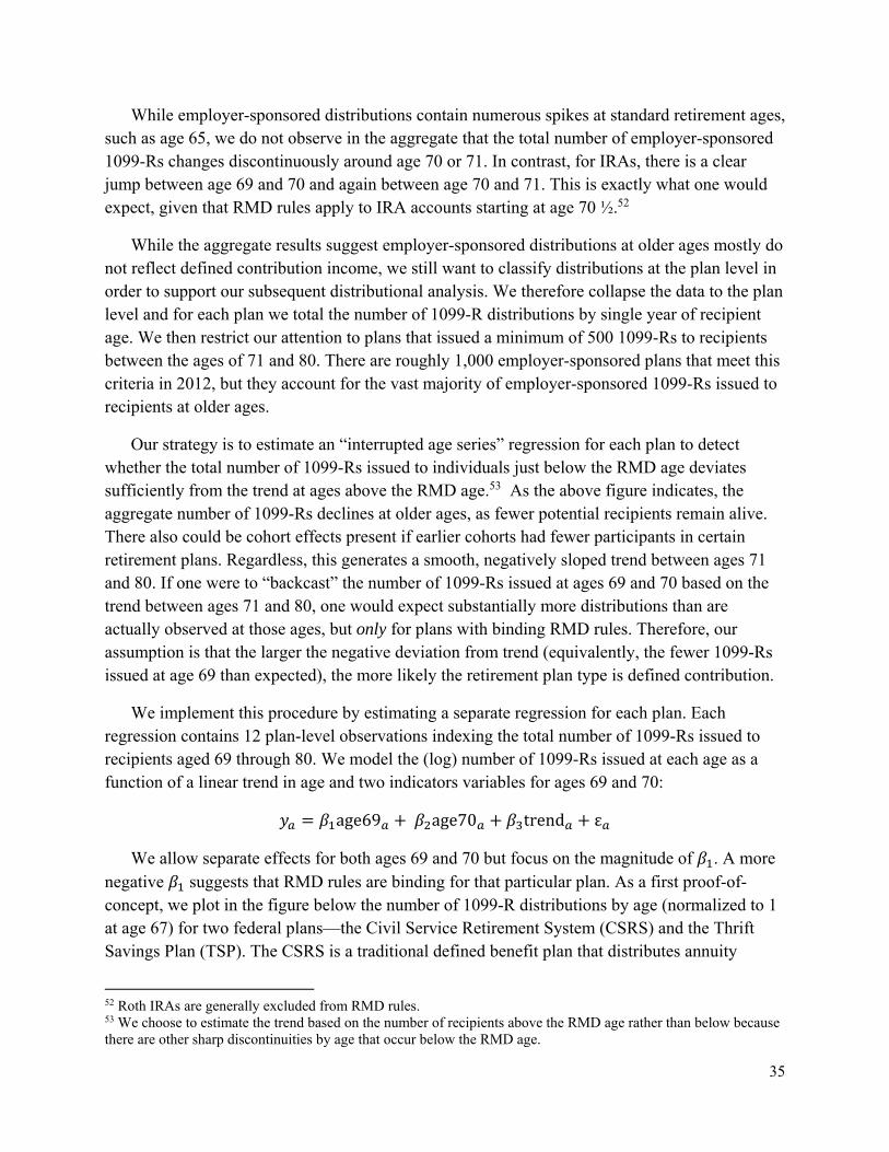
35  

While employer-sponsored distributions contain numerous spikes at standard retirement ages, such as age 65, we do not observe in the aggregate that the total number of employer-sponsored 1099-Rs changes discontinuously around age 70 or 71. In contrast, for IRAs, there is a clear jump between age 69 and 70 and again between age 70 and 71. This is exactly what one would expect, given that RMD rules apply to IRA accounts starting at age 70 ½.52

While the aggregate results suggest employer-sponsored distributions at older ages mostly do not reflect defined contribution income, we still want to classify distributions at the plan level in order to support our subsequent distributional analysis. We therefore collapse the data to the plan level and for each plan we total the number of 1099-R distributions by single year of recipient age. We then restrict our attention to plans that issued a minimum of 500 1099-Rs to recipients between the ages of 71 and 80. There are roughly 1,000 employer-sponsored plans that meet this criteria in 2012, but they account for the vast majority of employer-sponsored 1099-Rs issued to recipients at older ages.

Our strategy is to estimate an “interrupted age series” regression for each plan to detect whether the total number of 1099-Rs issued to individuals just below the RMD age deviates sufficiently from the trend at ages above the RMD age.53 As the above figure indicates, the aggregate number of 1099-Rs declines at older ages, as fewer potential recipients remain alive. There also could be cohort effects present if earlier cohorts had fewer participants in certain retirement plans. Regardless, this generates a smooth, negatively sloped trend between ages 71 and 80. If one were to “backcast” the number of 1099-Rs issued at ages 69 and 70 based on the trend between ages 71 and 80, one would expect substantially more distributions than are actually observed at those ages, but only for plans with binding RMD rules. Therefore, our assumption is that the larger the negative deviation from trend (equivalently, the fewer 1099-Rs issued at age 69 than expected), the more likely the retirement plan type is defined contribution.

We implement this procedure by estimating a separate regression for each plan. Each regression contains 12 plan-level observations indexing the total number of 1099-Rs issued to recipients aged 69 through 80. We model the (log) number of 1099-Rs issued at each age as a function of a linear trend in age and two indicators variables for ages 69 and 70:

age69 age70 trend ε

We allow separate effects for both ages 69 and 70 but focus on the magnitude of . A more negative suggests that RMD rules are binding for that particular plan. As a first proof-of-concept, we plot in the figure below the number of 1099-R distributions by age (normalized to 1 at age 67) for two federal plans—the Civil Service Retirement System (CSRS) and the Thrift Savings Plan (TSP). The CSRS is a traditional defined benefit plan that distributes annuity

                                                            52 Roth IRAs are generally excluded from RMD rules. 53 We choose to estimate the trend based on the number of recipients above the RMD age rather than below because there are other sharp discontinuities by age that occur below the RMD age.

 

36  

income while the TSP is a defined contribution plan that is similar in many aspects to 401(k) plans in the private sector.

Methods Appendix Figure 2. CSRS and TSP recipiency by age: 2012

Source: 2013 CPS ASEC linked to IRS Form 1099-R records.

As the figure above indicates, there is little trend in the number of 1099-Rs issued by CSRS across ages. This is consistent with a lack of relevance of RMD rules for defined benefit plans. In contrast, there is a clear jump in the number of 1099-Rs issued by the TSP around the RMD age, which is consistent with its defined contribution status. The estimated equations for both plans reflect the visual evidence.

We next plot the distribution of across all employer-sponsored plans. As a second proof- of-concept we also implement the above regression analysis and estimate for IRA plans, even though we are primarily interested in classifying employer-sponsored plans. Because IRAs are also defined contribution accounts subject to RMD rules, they serve as a useful validation test of our method. The resulting distributions of are shown in the two figures below. In the first figure, the distributions are weighted by the underlying number of 1099-Rs issued by the plan between ages 71 and 80, while in the second figure the results are unweighted.

 

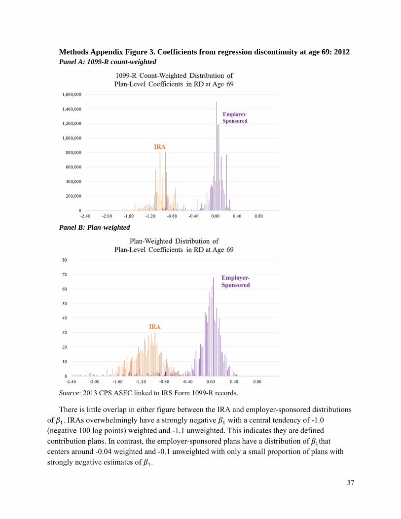
37  

Methods Appendix Figure 3. Coefficients from regression discontinuity at age 69: 2012 Panel A: 1099-R count-weighted

Panel B: Plan-weighted

Source: 2013 CPS ASEC linked to IRS Form 1099-R records.

There is little overlap in either figure between the IRA and employer-sponsored distributions of . IRAs overwhelmingly have a strongly negative with a central tendency of -1.0 (negative 100 log points) weighted and -1.1 unweighted. This indicates they are defined contribution plans. In contrast, the employer-sponsored plans have a distribution of that centers around -0.04 weighted and -0.1 unweighted with only a small proportion of plans with strongly negative estimates of .

 

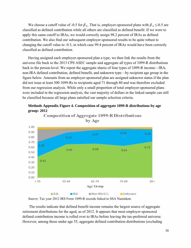
38  

We choose a cutoff value of -0.5 for . That is, employer-sponsored plans with ≤-0.5 are classified as defined contribution while all others are classified as defined benefit. If we were to apply this same cutoff to IRAs, we would correctly assign 98.2 percent of IRAs as defined contribution. We also find our subsequent employer-sponsored results to be quite robust to changing the cutoff value to -0.3, in which case 99.4 percent of IRAs would have been correctly classified as defined contribution.

Having assigned each employer-sponsored plan a type, we then link the results from the universe file back to the 2013 CPS ASEC sample and aggregate all types of 1099-R distributions back to the person-level. We report the aggregate shares of four types of 1099-R income—IRA, non-IRA defined contribution, defined benefit, and unknown type—by recipient age group in the figure below. Amounts from an employer-sponsored plan are assigned unknown status if the plan did not issue at least 500 1099-Rs to recipients aged 71 through 80 and was therefore excluded from our regression analysis. While only a small proportion of total employer-sponsored plans were included in the regression analysis, the vast majority of dollars in the linked sample can still be classified because all large plans satisfied our sample selection criteria.

Methods Appendix Figure 4. Composition of aggregate 1099-R distributions by age group: 2012

Source: Tax year 2012 IRS Form 1099-R records linked to SSA Numident.

The results indicate that defined benefit income remains the largest source of aggregate retirement distributions for the aged, as of 2012. It appears that most employer-sponsored defined contribution income is rolled over to IRAs before leaving the tax-preferred universe. However, among those under age 55, aggregate defined contribution distributions (excluding

 

39  

rollovers) play a larger role. This is consistent with the private sector transition away from defined benefit plans.

Having identified the different types of retirement distributions, we examine how the prevalence of each type varies across the income distribution. We discuss these results in Section V.10 of the main text.

Table 1. Aggregate income estimates by age group: 2012(In billions, 2012 dollars)

Aged 18 to 64

Aged 65 and Over

Aged 18 to 64

Aged 65 and Over

Aged 18 to 64

Aged 65 and Over

Aged 18 to 64

Aged 65 and Over

Earnings 6,659 415 6,651 399 6,633 406 100.3% 98.1%Social Security 132 517 124 525 150 545 83.1% 96.2%Supplemental Security Income 36 7 37 7 30 10 123.2% 72.7%Interest and dividends 158 113 159 116 206 184 77.4% 63.1%Retirement income 182 279 178 283 396 595 44.9% 47.6% IRAs (from Form 1099-R) 108 171 Employer sponsored (from Form 1099-R) 288 424

Income from all five sources 7,167 1,332 7,149 1,330 7,415 1,740 96.4% 76.4%

Weighted count (thousands of persons) 193,642 43,287 191,930 43,217 191,930 43,217N (persons) 122,316 23,446 107,903 21,239 107,903 21,239

CPS as % of Admin(2) / (3)

(4)

CPS PIK SampleFull CPS Sample

Linked CPS-Admin

Sample

(1) (2) (3)

Source : 2013 CPS ASEC linked to SSA and IRS administrative records.Notes : The Full CPS Sample (column 1) consists of all CPS persons within one of two age groups—aged 18 to 64 and aged 65 and over—and uses only survey-based values to calculate income aggregates for those two age groups. The CPS PIK Sample (column 2) is a subset of the Full CPS Sample and includes only persons who are assigned a Personal Identification Key (PIK) that allows linking to administrative records, but the CPS PIK Sample continues to use only survey-based values to calculate income aggregates. The Linked CPS-Admin Sample (column 3) is the same set of people as the CPS PIK Sample except administrative record values for each of five types of income have been used to calculate income aggregates. Retirement income includes retirement, survivor, and disability pensions (excluding Social Security) as well as defined contribution account withdrawals. CPS ASEC final person weights are used for the Full CPS Sample. For the CPS PIK Sample and the Linked CPS-Admin Sample we adjust the final person weights to account for selection into having a PIK. We first estimate a logit model for the presence of a PIK as a function of CPS demographic characteristics and predict the propensity score. We then take the CPS sample weight and multiply it by the inverse of the propensity score. The resulting weights are used for the CPS PIK Sample and the Linked CPS-Admin Sample.

40

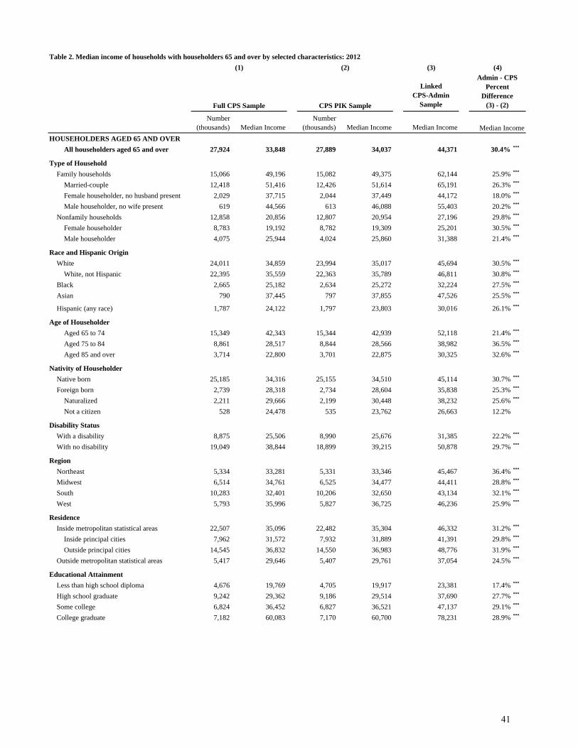
(3)

Linked CPS-Admin

Sample

Number (thousands) Median Income

Number (thousands) Median Income Median Income

HOUSEHOLDERS AGED 65 AND OVER

All householders aged 65 and over 27,924 33,848 27,889 34,037 44,371 30.4% ***

Type of Household

Family households 15,066 49,196 15,082 49,375 62,144 25.9% ***

Married-couple 12,418 51,416 12,426 51,614 65,191 26.3% ***

Female householder, no husband present 2,029 37,715 2,044 37,449 44,172 18.0% ***

Male householder, no wife present 619 44,566 613 46,088 55,403 20.2% ***

Nonfamily households 12,858 20,856 12,807 20,954 27,196 29.8% ***

Female householder 8,783 19,192 8,782 19,309 25,201 30.5% ***

Male householder 4,075 25,944 4,024 25,860 31,388 21.4% ***

Race and Hispanic Origin

White 24,011 34,859 23,994 35,017 45,694 30.5% ***

White, not Hispanic 22,395 35,559 22,363 35,789 46,811 30.8% ***

Black 2,665 25,182 2,634 25,272 32,224 27.5% ***

Asian 790 37,445 797 37,855 47,526 25.5% ***

Hispanic (any race) 1,787 24,122 1,797 23,803 30,016 26.1% ***

Age of Householder

Aged 65 to 74 15,349 42,343 15,344 42,939 52,118 21.4% ***

Aged 75 to 84 8,861 28,517 8,844 28,566 38,982 36.5% ***

Aged 85 and over 3,714 22,800 3,701 22,875 30,325 32.6% ***

Nativity of Householder

Native born 25,185 34,316 25,155 34,510 45,114 30.7% ***

Foreign born 2,739 28,318 2,734 28,604 35,838 25.3% ***

Naturalized 2,211 29,666 2,199 30,448 38,232 25.6% ***

Not a citizen 528 24,478 535 23,762 26,663 12.2%

Disability Status

With a disability 8,875 25,506 8,990 25,676 31,385 22.2% ***

With no disability 19,049 38,844 18,899 39,215 50,878 29.7% ***

Region

Northeast 5,334 33,281 5,331 33,346 45,467 36.4% ***

Midwest 6,514 34,761 6,525 34,477 44,411 28.8% ***

South 10,283 32,401 10,206 32,650 43,134 32.1% ***

West 5,793 35,996 5,827 36,725 46,236 25.9% ***

Residence

Inside metropolitan statistical areas 22,507 35,096 22,482 35,304 46,332 31.2% ***

Inside principal cities 7,962 31,572 7,932 31,889 41,391 29.8% ***

Outside principal cities 14,545 36,832 14,550 36,983 48,776 31.9% ***

Outside metropolitan statistical areas 5,417 29,646 5,407 29,761 37,054 24.5% ***

Educational Attainment

Less than high school diploma 4,676 19,769 4,705 19,917 23,381 17.4% ***

High school graduate 9,242 29,362 9,186 29,514 37,690 27.7% ***

Some college 6,824 36,452 6,827 36,521 47,137 29.1% ***

College graduate 7,182 60,083 7,170 60,700 78,231 28.9% ***

Table 2. Median income of households with householders 65 and over by selected characteristics: 2012

Median Income

(1) (2) (4)

Full CPS Sample CPS PIK Sample

Admin - CPS Percent

Difference(3) - (2)

41

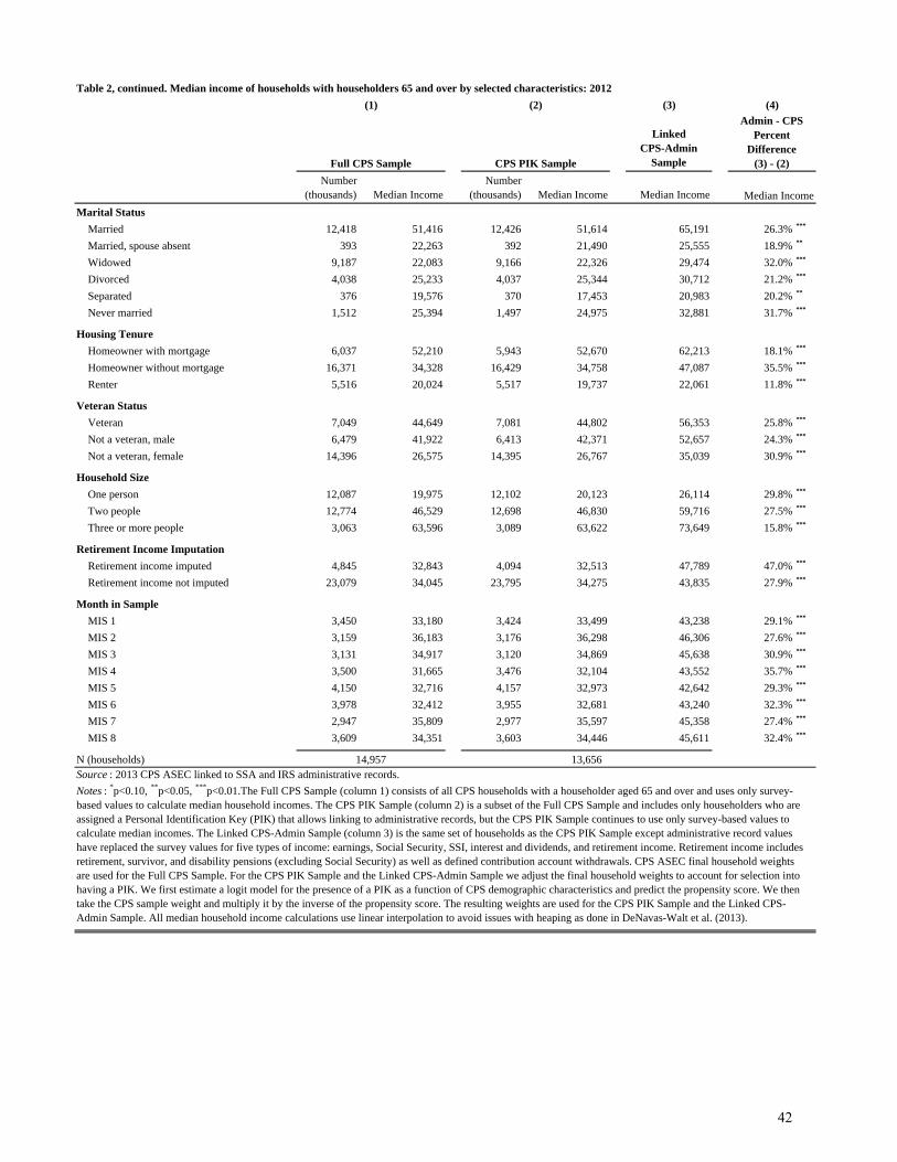
Table 2, continued. Median income of households with householders 65 and over by selected characteristics: 2012

(3)

Linked CPS-Admin

Sample

Number (thousands) Median Income

Number (thousands) Median Income Median Income

Marital Status

Married 12,418 51,416 12,426 51,614 65,191 26.3% ***

Married, spouse absent 393 22,263 392 21,490 25,555 18.9% **

Widowed 9,187 22,083 9,166 22,326 29,474 32.0% ***

Divorced 4,038 25,233 4,037 25,344 30,712 21.2% ***

Separated 376 19,576 370 17,453 20,983 20.2% **

Never married 1,512 25,394 1,497 24,975 32,881 31.7% ***

Housing Tenure

Homeowner with mortgage 6,037 52,210 5,943 52,670 62,213 18.1% ***

Homeowner without mortgage 16,371 34,328 16,429 34,758 47,087 35.5% ***

Renter 5,516 20,024 5,517 19,737 22,061 11.8% ***

Veteran Status

Veteran 7,049 44,649 7,081 44,802 56,353 25.8% ***

Not a veteran, male 6,479 41,922 6,413 42,371 52,657 24.3% ***

Not a veteran, female 14,396 26,575 14,395 26,767 35,039 30.9% ***

Household Size

One person 12,087 19,975 12,102 20,123 26,114 29.8% ***

Two people 12,774 46,529 12,698 46,830 59,716 27.5% ***

Three or more people 3,063 63,596 3,089 63,622 73,649 15.8% ***

Retirement Income Imputation

Retirement income imputed 4,845 32,843 4,094 32,513 47,789 47.0% ***

Retirement income not imputed 23,079 34,045 23,795 34,275 43,835 27.9% ***

Month in Sample

MIS 1 3,450 33,180 3,424 33,499 43,238 29.1% ***

MIS 2 3,159 36,183 3,176 36,298 46,306 27.6% ***

MIS 3 3,131 34,917 3,120 34,869 45,638 30.9% ***

MIS 4 3,500 31,665 3,476 32,104 43,552 35.7% ***

MIS 5 4,150 32,716 4,157 32,973 42,642 29.3% ***

MIS 6 3,978 32,412 3,955 32,681 43,240 32.3% ***

MIS 7 2,947 35,809 2,977 35,597 45,358 27.4% ***

MIS 8 3,609 34,351 3,603 34,446 45,611 32.4% ***

N (households)Source : 2013 CPS ASEC linked to SSA and IRS administrative records.Notes : *p<0.10, **p<0.05, ***p<0.01.The Full CPS Sample (column 1) consists of all CPS households with a householder aged 65 and over and uses only survey-based values to calculate median household incomes. The CPS PIK Sample (column 2) is a subset of the Full CPS Sample and includes only householders who are assigned a Personal Identification Key (PIK) that allows linking to administrative records, but the CPS PIK Sample continues to use only survey-based values to calculate median incomes. The Linked CPS-Admin Sample (column 3) is the same set of households as the CPS PIK Sample except administrative record values have replaced the survey values for five types of income: earnings, Social Security, SSI, interest and dividends, and retirement income. Retirement income includes retirement, survivor, and disability pensions (excluding Social Security) as well as defined contribution account withdrawals. CPS ASEC final household weights are used for the Full CPS Sample. For the CPS PIK Sample and the Linked CPS-Admin Sample we adjust the final household weights to account for selection into having a PIK. We first estimate a logit model for the presence of a PIK as a function of CPS demographic characteristics and predict the propensity score. We then take the CPS sample weight and multiply it by the inverse of the propensity score. The resulting weights are used for the CPS PIK Sample and the Linked CPS-Admin Sample. All median household income calculations use linear interpolation to avoid issues with heaping as done in DeNavas-Walt et al. (2013).

Full CPS Sample CPS PIK Sample

Admin - CPS Percent

Difference(3) - (2)

Median Income

(4)

14,957 13,656

(1) (2)

42

Table 3. People in poverty by selected characteristics, among people aged 65 and over: 2012

(Numbers in thousands.)

Total Number Percent Total Number Percent Number Percent NumberPEOPLE AGED 65 AND OVER

Total 43,287 3,926 9.1 43,217 3,879 9.0 2,992 6.9 -887 -2.1 ***

Family Status

In families 29,761 1,593 5.4 29,748 1,586 5.3 1,016 3.4 -570 -1.9 ***

Householder 15,067 826 5.5 15,082 810 5.4 549 3.6 -261 -1.7 ***

Unrelated individuals 13,516 2,332 17.3 13,456 2,292 17.0 1,970 14.6 -322 -2.4 ***

Race and Hispanic Origin

White 37,039 2,891 7.8 37,008 2,842 7.7 2,156 5.8 -686 -1.9 ***

White, not Hispanic 34,131 2,324 6.8 34,089 2,265 6.6 1,630 4.8 -635 -1.9 ***

Black 3,893 708 18.2 3,855 711 18.4 539 14.0 -172 -4.4 ***

Asian 1,669 205 12.3 1,669 207 12.4 194 11.7 -13 -0.7

Hispanic (any race) 3,213 663 20.6 3,211 670 20.9 613 19.1 -57 -1.8

Sex

Male 19,298 1,282 6.6 19,264 1,282 6.7 949 4.9 -333 -1.7 ***

Female 23,990 2,643 11.0 23,954 2,596 10.8 2,043 8.5 -553 -2.3 ***

Age

Aged 65 to 74 24,702 1,960 7.9 24,668 1,937 7.9 1,665 6.7 -272 -1.1 ***

Aged 75 to 84 13,289 1,316 9.9 13,278 1,302 9.8 924 7.0 -378 -2.8 ***

Aged 85 and over 5,296 649 12.3 5,271 640 12.1 403 7.6 -237 -4.5 ***

Nativity

Native born 38,077 3,078 8.1 38,027 3,035 8.0 2,148 5.6 -887 -2.3 ***

Foreign born 5,211 848 16.3 5,190 844 16.3 843 16.2 -1 0.0Naturalized 3,877 563 14.5 3,857 559 14.5 544 14.1 -15 -0.4Not a citizen 1,334 285 21.4 1,333 285 21.4 300 22.5 15 1.1

Region

Northeast 8,121 760 9.4 8,125 761 9.4 595 7.3 -166 -2.0 ***

Midwest 9,771 664 6.8 9,750 649 6.7 465 4.8 -184 -1.9 ***

South 16,150 1,648 10.2 16,051 1,625 10.1 1,231 7.7 -394 -2.5 ***

West 9,245 853 9.2 9,291 843 9.1 701 7.5 -142 -1.5 **

Residence

Inside metropolitan statistical areas 35,120 3,159 9.0 35,044 3,109 8.9 2,303 6.6 -806 -2.3 ***

Inside principal cities 12,077 1,506 12.5 12,001 1,490 12.4 1,219 10.2 -271 -2.3 ***

Outside principal cities 23,043 1,653 7.2 23,043 1,618 7.0 1,084 4.7 -534 -2.3 ***

Outside metropolitan statistical areas 8,167 767 9.4 8,173 770 9.4 689 8.4 -81 -1.0 *

Disability Status

With a disability 13,301 1,727 13.0 13,520 1,735 12.8 1,466 10.8 -269 -2.0 ***

With no disability 29,987 2,199 7.3 29,697 2,144 7.2 1,526 5.1 -618 -2.1 ***

Educational Attainment

Less than high school diploma 7,547 1,526 20.2 7,560 1,539 20.4 1,374 18.2 -165 -2.2 ***

High school graduate 15,120 1,295 8.6 15,081 1,295 8.6 889 5.9 -406 -2.7 ***

Some college 9,675 600 6.2 9,679 589 6.1 443 4.6 -146 -1.5 ***

College graduate 10,945 504 4.6 10,899 457 4.2 285 2.6 -172 -1.6 ***

Below Poverty Below Poverty Below Poverty Below Poverty

(1) (2) (3) (4)

Full CPS Sample CPS PIK Sample

Linked CPS-Admin

Sample

Admin - CPS Difference

(3) - (2)

Points

43

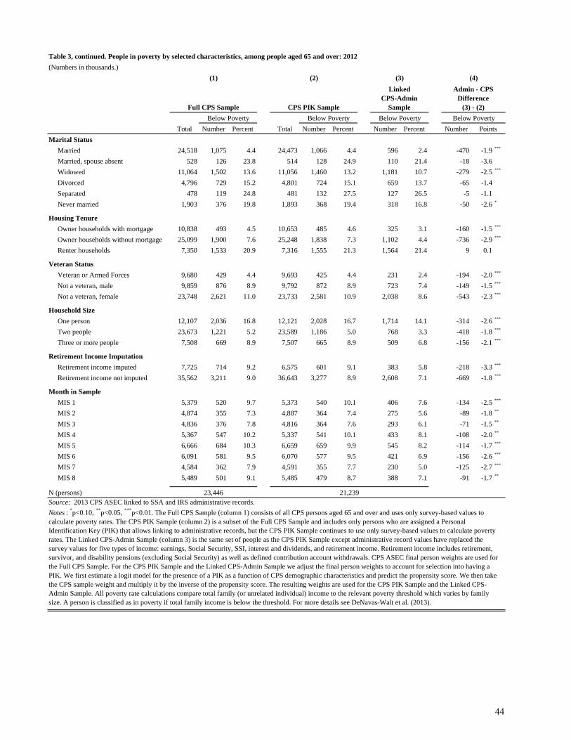
Table 3, continued. People in poverty by selected characteristics, among people aged 65 and over: 2012

(Numbers in thousands.)

Total Number Percent Total Number Percent Number Percent NumberMarital Status

Married 24,518 1,075 4.4 24,473 1,066 4.4 596 2.4 -470 -1.9 ***

Married, spouse absent 528 126 23.8 514 128 24.9 110 21.4 -18 -3.6Widowed 11,064 1,502 13.6 11,056 1,460 13.2 1,181 10.7 -279 -2.5 ***

Divorced 4,796 729 15.2 4,801 724 15.1 659 13.7 -65 -1.4Separated 478 119 24.8 481 132 27.5 127 26.5 -5 -1.1Never married 1,903 376 19.8 1,893 368 19.4 318 16.8 -50 -2.6 *

Housing Tenure

Owner households with mortgage 10,838 493 4.5 10,653 485 4.6 325 3.1 -160 -1.5 ***

Owner households without mortgage 25,099 1,900 7.6 25,248 1,838 7.3 1,102 4.4 -736 -2.9 ***

Renter households 7,350 1,533 20.9 7,316 1,555 21.3 1,564 21.4 9 0.1

Veteran Status

Veteran or Armed Forces 9,680 429 4.4 9,693 425 4.4 231 2.4 -194 -2.0 ***

Not a veteran, male 9,859 876 8.9 9,792 872 8.9 723 7.4 -149 -1.5 ***

Not a veteran, female 23,748 2,621 11.0 23,733 2,581 10.9 2,038 8.6 -543 -2.3 ***

Household Size

One person 12,107 2,036 16.8 12,121 2,028 16.7 1,714 14.1 -314 -2.6 ***

Two people 23,673 1,221 5.2 23,589 1,186 5.0 768 3.3 -418 -1.8 ***

Three or more people 7,508 669 8.9 7,507 665 8.9 509 6.8 -156 -2.1 ***

Retirement Income Imputation

Retirement income imputed 7,725 714 9.2 6,575 601 9.1 383 5.8 -218 -3.3 ***

Retirement income not imputed 35,562 3,211 9.0 36,643 3,277 8.9 2,608 7.1 -669 -1.8 ***

Month in Sample

MIS 1 5,379 520 9.7 5,373 540 10.1 406 7.6 -134 -2.5 ***

MIS 2 4,874 355 7.3 4,887 364 7.4 275 5.6 -89 -1.8 **

MIS 3 4,836 376 7.8 4,816 364 7.6 293 6.1 -71 -1.5 **

MIS 4 5,367 547 10.2 5,337 541 10.1 433 8.1 -108 -2.0 **

MIS 5 6,666 684 10.3 6,659 659 9.9 545 8.2 -114 -1.7 ***

MIS 6 6,091 581 9.5 6,070 577 9.5 421 6.9 -156 -2.6 ***

MIS 7 4,584 362 7.9 4,591 355 7.7 230 5.0 -125 -2.7 ***

MIS 8 5,489 501 9.1 5,485 479 8.7 388 7.1 -91 -1.7 **

N (persons) 23,446 21,239Source: 2013 CPS ASEC linked to SSA and IRS administrative records.Notes : *p<0.10, **p<0.05, ***p<0.01. The Full CPS Sample (column 1) consists of all CPS persons aged 65 and over and uses only survey-based values to calculate poverty rates. The CPS PIK Sample (column 2) is a subset of the Full CPS Sample and includes only persons who are assigned a Personal Identification Key (PIK) that allows linking to administrative records, but the CPS PIK Sample continues to use only survey-based values to calculate poverty rates. The Linked CPS-Admin Sample (column 3) is the same set of people as the CPS PIK Sample except administrative record values have replaced the survey values for five types of income: earnings, Social Security, SSI, interest and dividends, and retirement income. Retirement income includes retirement, survivor, and disability pensions (excluding Social Security) as well as defined contribution account withdrawals. CPS ASEC final person weights are used for the Full CPS Sample. For the CPS PIK Sample and the Linked CPS-Admin Sample we adjust the final person weights to account for selection into having a PIK. We first estimate a logit model for the presence of a PIK as a function of CPS demographic characteristics and predict the propensity score. We then take the CPS sample weight and multiply it by the inverse of the propensity score. The resulting weights are used for the CPS PIK Sample and the Linked CPS-Admin Sample. All poverty rate calculations compare total family (or unrelated individual) income to the relevant poverty threshold which varies by family size. A person is classified as in poverty if total family income is below the threshold. For more details see DeNavas-Walt et al. (2013).

(1) (2) (3) (4)

Full CPS Sample CPS PIK Sample

Linked CPS-Admin

Sample

Admin - CPS Difference

(3) - (2)

Below Poverty Below Poverty Below Poverty Below PovertyPoints

44

Panel A: Substituting one additional source at a time

(1) (2) (3) (4) (5) (6) (7)

CPS PIK Sample

(Baseline Values)

Sub Earnings

+Sub Social

Security +Sub SSI

+Sub Interest

and Dividends

+Sub Retirement

Income

Linked CPS-Admin

Sample (Final

Values)

Householders aged 65 and over5th percentile 8,543 0.15% -2.61% 2.98% 5.32% 11.89% 9,55910th 11,661 -0.05% 2.07% 2.45% 5.46% 12.74% 13,14625th 18,857 0.26% 1.75% 1.84% 6.71% 25.53% 23,672Median 34,037 -0.10% 1.89% 1.68% 5.79% 30.36% 44,37175th 63,322 -1.85% -0.94% -1.17% 0.55% 22.10% 77,31490th 108,369 -0.96% -0.42% -0.65% -1.93% 14.49% 124,06995th 145,182 0.05% 1.67% 1.81% 0.52% 16.00% 168,411

Mean 51,736 1.09% 2.51% 2.55% 7.04% 27.91% 66,177

Gini coefficient 0.473 0.482 0.479 0.479 0.487 0.489 0.489

People aged 65 and over0-50% of poverty threshold 0.026 0.000 0.001 -0.006 -0.007 -0.011 0.0150-100% 0.090 0.001 -0.003 -0.005 -0.009 -0.021 0.0690-150% 0.208 -0.001 -0.016 -0.016 -0.027 -0.060 0.1480-200% 0.334 0.001 -0.016 -0.015 -0.034 -0.098 0.236

N (households)N (persons)

Table 4. Cumulative income and poverty depth differences between CPS ASEC and administrative records: 2012

Percent Change in Household Income at Select Percentiles

Change in Proportion with Family Incomes Below Specified Ratio of Poverty Threshold

13,65621,239

45

(1) (2) (3) (4) (5) (6)CPS PIK Sample

(Baseline Values)

Sub Only Earnings

Sub Only Social

SecuritySub Only

SSI

Sub OnlyInterest

andDividends

Sub Only Retirement

Income

Householders aged 65 and over5th percentile 8,543 0.15% -2.68% 0.68% 4.81% 13.26%10th 11,661 -0.05% 2.23% 1.58% 4.02% 11.64%25th 18,857 0.26% 1.26% 0.40% 5.02% 18.21%Median 34,037 -0.10% 2.61% -0.14% 4.45% 24.54%75th 63,322 -1.85% 1.10% -0.14% 1.75% 21.46%90th 108,369 -0.96% 0.30% -0.12% -1.49% 15.29%95th 145,182 0.05% 1.63% 0.00% -2.17% 15.39%

Mean 51,736 1.09% 1.42% 0.04% 4.49% 20.88%

Gini index 0.473 0.482 0.471 0.473 0.480 0.476

People aged 65 and over0-50% of poverty threshold 0.026 0.000 0.002 0.001 -0.003 -0.0070-100% 0.090 0.001 -0.004 -0.003 -0.008 -0.0180-150% 0.208 -0.001 -0.015 -0.003 -0.013 -0.0480-200% 0.334 0.001 -0.017 -0.001 -0.020 -0.078

N (households)N (persons)

Change in Proportion with Family Incomes Below Specified Ratio of Poverty Threshold

Source : 2013 CPS ASEC linked to SSA and IRS administrative records. Notes: The top section of the table analyzes household income quantiles. The CPS PIK Sample (Baseline Values) in column 1 consists of all CPS households with a householder aged 65 and over who are assigned a Protection Identification Key (PIK) that allows linking to administrative records, but uses only survey-based values to calculate household income quantiles. Each subsequent column maintains the same set of households but replaces one source of survey-based income with its administrative counterpart. In Panel A, income sources are replaced one at a time in a cumulative fashion and in each column households are re-ranked based on the new measure of income. Five types of income are replaced: earnings, Social Security, SSI, interest and dividends, and retirement income. Retirement income includes retirement, survivor, and disability pensions (excluding Social Security) as well as defined contribution account withdrawals. After a new set of household income quantiles is estimated, the percentage change relative to baseline values is calculated. The Linked CPS-Admin Sample (Final Values) in column 7 represents the cumulative effect (expressed in levels) of replacing all five types of survey-based income with administrative counterparts.The bottom half of the table analyzes the distribution of persons across various income-to-poverty ratio intervals. An income-to poverty ratio is calculated as a person’s total family (or unrelated individual) income divided by the relevant poverty threshold which varies based on family size. See DeNavas-Walt et al. (2013) for more details. The CPS PIK Sample (Baseline Values) in column 1 consists of all CPS persons aged 65 and over who are assigned a Protection Identification Key (PIK) that allows linking to administrative records, but uses only survey-based values to calculate income to poverty ratios. Each subsequent column maintains the same set of persons but replaces one source of survey-based income with its administrative counterpart. Five types of income are replaced: earnings, social security, SSI, interest and dividends, and retirement income. Retirement income includes retirement, survivor, and disability pensions (excluding Social Security) as well as defined contribution account withdrawals. Income sources are replaced one at a time in a cumulative fashion. In each column the distribution of persons across the various income to poverty ratio intervals is re-estimated, and the difference in the distribution relative to the baseline values is shown. The Linked CPS-Admin Sample (Final Values) in column 7 represents the cumulative effect (expressed in terms of the final distribution) of replacing all five types of survey-based income with administrative counterparts.All estimates make use of CPS final household/person weights. We adjust the weights to account for selection into having a PIK. We first estimate a logit model for the presence of a PIK as a function of CPS demographic characteristics and predict the propensity score. We then take the CPS sample weight and multiply it by the inverse of the propensity score. The resulting weights are used in the analysis.

Percent Change in Household Income at Select Percentiles

Panel B: Substituting one source only

13,65621,239

46

(1) (2) (3) (4) (5) (6) (7) (8)

CPS Baseline

Replace False

Positives

+Replace True

Positives

+Replace False

NegativesFalse

PositivesTrue

PositivesFalse

Negatives

+Replace All Other

Admin

Household income amounts, householders aged 65 and over

5th 8,543 8,234 8,285 9,653 -0.279 0.045 1.233 9,55910th 11,661 11,340 11,407 13,003 -0.239 0.050 1.189 13,14625th 18,857 18,281 18,743 22,256 -0.170 0.136 1.034 23,672Median 34,037 33,085 35,419 42,339 -0.115 0.281 0.833 44,37175th 63,322 62,153 67,326 76,808 -0.087 0.384 0.703 77,31490th 108,369 107,064 113,969 124,815 -0.079 0.420 0.660 124,06995th 145,182 144,423 153,979 167,338 -0.034 0.431 0.603 168,411

Mean 51,736 50,828 54,783 62,477 -0.085 0.368 0.716 66,177

Proportions below specified income-to-poverty ratios, people aged 65 and over

0-50% 0.026 0.029 0.029 0.019 -0.424 0.037 1.387 0.0150-100% 0.090 0.096 0.095 0.072 -0.381 0.108 1.273 0.0690-150% 0.208 0.219 0.211 0.161 -0.225 0.152 1.073 0.1480-200% 0.334 0.348 0.334 0.257 -0.175 0.183 0.993 0.236

Retirement income amounts (unconditional), people aged 65 and over

Median 1,834 1,754 1,792 2,991 -0.069 0.033 1.036 --Mean 6,559 5,962 8,617 13,770 -0.083 0.368 0.715 --

N (households)N (persons)

Table 5. Decomposition of intensive and extensive margins of retirement income misreporting: 2012

Source : 2013 CPS ASEC linked to SSA and IRS administrative records.Notes : The top section of the table analyzes household income quantiles. The CPS PIK Sample (Baseline Values) in column 1 consists of all CPS households with a householder aged 65 and over who are assigned a Protection Identification Key (PIK) that allows linking to administrative records, but uses only survey-based values to calculate household income quantiles. Each of the next three columns maintains the same set of households but uses the 1099-R administrative records to correct for one type of retirement income misreporting. After each correction, households are re-ranked based on the new measure of income. Corrections are made in a cumulative fashion. Column 2 replaces false positives with zeros, column 3 swaps the amounts in the survey for the amounts in the administrative records among those with positive amounts in both sources, and column 4 replaces the false negative reports with the amounts from the administrative records. Columns 5 through 7 compute the percentage of the overall change (relative to column 1) that is attributable to each type of misreporting. To put retirement income in context, column 8 then swaps the other four sources of survey income for their administrative record counterparts. The other four sources of income are: earnings, Social Security, SSI, and interest and dividends. The second section of the table performs the same exercise for the proportion of persons aged 65 and over (with a PIK) that are below specified intervals of the income-to-poverty ratio. An income-to poverty ratio is calculated as a person’s total family (or unrelated individual) income divided by the relevant poverty threshold which varies based on family size. See DeNavas-Walt et al. (2013) for more details. The third section of the table performs the same exercise for persons aged 65 and over (with a PIK) but examines the unconditional mean and median amounts of retirement income. All estimates make use of CPS final household/person weights. We adjust the weights to account for selection into having a PIK. We first estimate a logit model for the presence of a PIK as a function of CPS demographic characteristics and predict the propensity score. We then take the CPS sample weight and multiply it by the inverse of the propensity score. The resulting weights are used in the analysis.

Proportion of Total Difference from each Replacement

13,65621,239

47

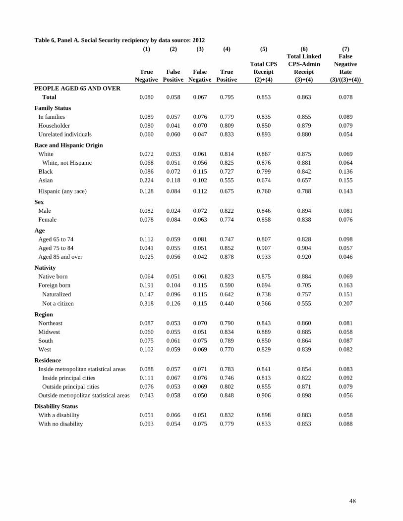
Table 6, Panel A. Social Security recipiency by data source: 2012

(1) (2) (3) (4) (5) (6) (7)

PEOPLE AGED 65 AND OVER

Total 0.080 0.058 0.067 0.795 0.853 0.863 0.078

Family Status

In families 0.089 0.057 0.076 0.779 0.835 0.855 0.089Householder 0.080 0.041 0.070 0.809 0.850 0.879 0.079Unrelated individuals 0.060 0.060 0.047 0.833 0.893 0.880 0.054

Race and Hispanic Origin

White 0.072 0.053 0.061 0.814 0.867 0.875 0.069White, not Hispanic 0.068 0.051 0.056 0.825 0.876 0.881 0.064

Black 0.086 0.072 0.115 0.727 0.799 0.842 0.136Asian 0.224 0.118 0.102 0.555 0.674 0.657 0.155

Hispanic (any race) 0.128 0.084 0.112 0.675 0.760 0.788 0.143

Sex

Male 0.082 0.024 0.072 0.822 0.846 0.894 0.081Female 0.078 0.084 0.063 0.774 0.858 0.838 0.076

Age

Aged 65 to 74 0.112 0.059 0.081 0.747 0.807 0.828 0.098Aged 75 to 84 0.041 0.055 0.051 0.852 0.907 0.904 0.057Aged 85 and over 0.025 0.056 0.042 0.878 0.933 0.920 0.046

Nativity

Native born 0.064 0.051 0.061 0.823 0.875 0.884 0.069Foreign born 0.191 0.104 0.115 0.590 0.694 0.705 0.163

Naturalized 0.147 0.096 0.115 0.642 0.738 0.757 0.151Not a citizen 0.318 0.126 0.115 0.440 0.566 0.555 0.207

Region

Northeast 0.087 0.053 0.070 0.790 0.843 0.860 0.081Midwest 0.060 0.055 0.051 0.834 0.889 0.885 0.058South 0.075 0.061 0.075 0.789 0.850 0.864 0.087West 0.102 0.059 0.069 0.770 0.829 0.839 0.082

Residence

Inside metropolitan statistical areas 0.088 0.057 0.071 0.783 0.841 0.854 0.083Inside principal cities 0.111 0.067 0.076 0.746 0.813 0.822 0.092Outside principal cities 0.076 0.053 0.069 0.802 0.855 0.871 0.079

Outside metropolitan statistical areas 0.043 0.058 0.050 0.848 0.906 0.898 0.056

Disability Status

With a disability 0.051 0.066 0.051 0.832 0.898 0.883 0.058With no disability 0.093 0.054 0.075 0.779 0.833 0.853 0.088

True Negative

Total Linked CPS-Admin

Receipt (3)+(4)

False Negative

Rate (3)/((3)+(4))

Total CPS Receipt (2)+(4)

False Positive

False Negative

True Positive

48

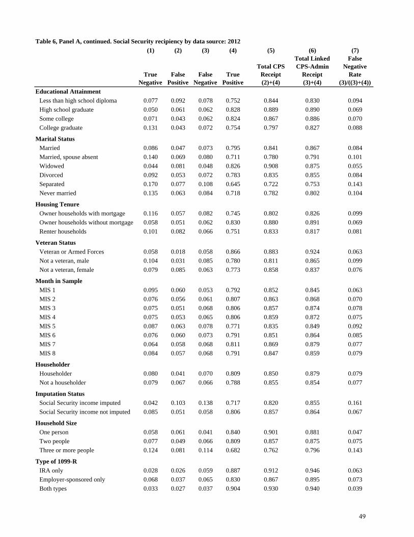
Table 6, Panel A, continued. Social Security recipiency by data source: 2012

(1) (2) (3) (4) (5) (6) (7)

Educational Attainment

Less than high school diploma 0.077 0.092 0.078 0.752 0.844 0.830 0.094High school graduate 0.050 0.061 0.062 0.828 0.889 0.890 0.069Some college 0.071 0.043 0.062 0.824 0.867 0.886 0.070College graduate 0.131 0.043 0.072 0.754 0.797 0.827 0.088

Marital Status

Married 0.086 0.047 0.073 0.795 0.841 0.867 0.084Married, spouse absent 0.140 0.069 0.080 0.711 0.780 0.791 0.101Widowed 0.044 0.081 0.048 0.826 0.908 0.875 0.055Divorced 0.092 0.053 0.072 0.783 0.835 0.855 0.084Separated 0.170 0.077 0.108 0.645 0.722 0.753 0.143Never married 0.135 0.063 0.084 0.718 0.782 0.802 0.104

Housing Tenure

Owner households with mortgage 0.116 0.057 0.082 0.745 0.802 0.826 0.099Owner households without mortgage 0.058 0.051 0.062 0.830 0.880 0.891 0.069Renter households 0.101 0.082 0.066 0.751 0.833 0.817 0.081

Veteran Status

Veteran or Armed Forces 0.058 0.018 0.058 0.866 0.883 0.924 0.063Not a veteran, male 0.104 0.031 0.085 0.780 0.811 0.865 0.099Not a veteran, female 0.079 0.085 0.063 0.773 0.858 0.837 0.076

Month in Sample

0.095 0.060 0.053 0.792 0.852 0.845 0.0630.076 0.056 0.061 0.807 0.863 0.868 0.0700.075 0.051 0.068 0.806 0.857 0.874 0.0780.075 0.053 0.065 0.806 0.859 0.872 0.0750.087 0.063 0.078 0.771 0.835 0.849 0.0920.076 0.060 0.073 0.791 0.851 0.864 0.0850.064 0.058 0.068 0.811 0.869 0.879 0.0770.084 0.057 0.068 0.791 0.847 0.859 0.079

Householder

Householder 0.080 0.041 0.070 0.809 0.850 0.879 0.079Not a householder 0.079 0.067 0.066 0.788 0.855 0.854 0.077

Imputation Status

Social Security income imputed 0.042 0.103 0.138 0.717 0.820 0.855 0.161Social Security income not imputed 0.085 0.051 0.058 0.806 0.857 0.864 0.067

Household Size

One person 0.058 0.061 0.041 0.840 0.901 0.881 0.047Two people 0.077 0.049 0.066 0.809 0.857 0.875 0.075Three or more people 0.124 0.081 0.114 0.682 0.762 0.796 0.143

Type of 1099-R

IRA only 0.028 0.026 0.059 0.887 0.912 0.946 0.063Employer-sponsored only 0.068 0.037 0.065 0.830 0.867 0.895 0.073Both types 0.033 0.027 0.037 0.904 0.930 0.940 0.039

MIS 3MIS 4MIS 5MIS 6

MIS 1MIS 2

MIS 8MIS 7

True Negative

Total Linked CPS-Admin

Receipt (3)+(4)

False Negative

Rate (3)/((3)+(4))

Total CPS Receipt (2)+(4)

False Positive

False Negative

True Positive

49

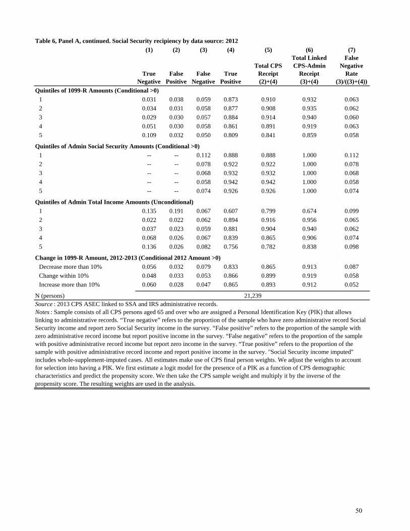
Table 6, Panel A, continued. Social Security recipiency by data source: 2012

(1) (2) (3) (4) (5) (6) (7)

Quintiles of 1099-R Amounts (Conditional >0)

0.031 0.038 0.059 0.873 0.910 0.932 0.0630.034 0.031 0.058 0.877 0.908 0.935 0.0620.029 0.030 0.057 0.884 0.914 0.940 0.0600.051 0.030 0.058 0.861 0.891 0.919 0.0630.109 0.032 0.050 0.809 0.841 0.859 0.058

Quintiles of Admin Social Security Amounts (Conditional >0)

-- -- 0.112 0.888 0.888 1.000 0.112-- -- 0.078 0.922 0.922 1.000 0.078-- -- 0.068 0.932 0.932 1.000 0.068-- -- 0.058 0.942 0.942 1.000 0.058-- -- 0.074 0.926 0.926 1.000 0.074

Quintiles of Admin Total Income Amounts (Unconditional)

0.135 0.191 0.067 0.607 0.799 0.674 0.0990.022 0.022 0.062 0.894 0.916 0.956 0.0650.037 0.023 0.059 0.881 0.904 0.940 0.0620.068 0.026 0.067 0.839 0.865 0.906 0.0740.136 0.026 0.082 0.756 0.782 0.838 0.098

Change in 1099-R Amount, 2012-2013 (Conditional 2012 Amount >0)

Decrease more than 10% 0.056 0.032 0.079 0.833 0.865 0.913 0.087Change within 10% 0.048 0.033 0.053 0.866 0.899 0.919 0.058Increase more than 10% 0.060 0.028 0.047 0.865 0.893 0.912 0.052

N (persons)

False Negative

Rate (3)/((3)+(4))

True Negative

False Positive

False Negative

True Positive

Total CPS Receipt (2)+(4)

Total Linked CPS-Admin

Receipt (3)+(4)

Source : 2013 CPS ASEC linked to SSA and IRS administrative records. Notes : Sample consists of all CPS persons aged 65 and over who are assigned a Personal Identification Key (PIK) that allows linking to administrative records. “True negative” refers to the proportion of the sample who have zero administrative record Social Security income and report zero Social Security income in the survey. “False positive” refers to the proportion of the sample with zero administrative record income but report positive income in the survey. “False negative” refers to the proportion of the sample with positive administrative record income but report zero income in the survey. “True positive” refers to the proportion of the sample with positive administrative record income and report positive income in the survey. "Social Security income imputed" includes whole-supplement-imputed cases. All estimates make use of CPS final person weights. We adjust the weights to account for selection into having a PIK. We first estimate a logit model for the presence of a PIK as a function of CPS demographic characteristics and predict the propensity score. We then take the CPS sample weight and multiply it by the inverse of the propensity score. The resulting weights are used in the analysis.

12

21,239

345

1

2345

2345

1

50

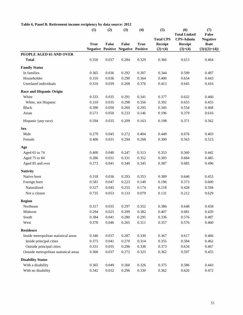
Table 6, Panel B. Retirement income recipiency by data source: 2012

(1) (2) (3) (4) (5) (6) (7)

PEOPLE AGED 65 AND OVER

Total 0.350 0.037 0.284 0.329 0.366 0.613 0.464

Family Status

In families 0.365 0.036 0.292 0.307 0.344 0.599 0.487Householder 0.310 0.036 0.290 0.364 0.400 0.654 0.443Unrelated individuals 0.316 0.039 0.268 0.376 0.415 0.645 0.416

Race and Hispanic Origin

White 0.333 0.035 0.291 0.341 0.377 0.632 0.460White, not Hispanic 0.310 0.035 0.298 0.356 0.392 0.655 0.455

Black 0.396 0.050 0.260 0.295 0.345 0.554 0.468Asian 0.571 0.050 0.233 0.146 0.196 0.379 0.616

Hispanic (any race) 0.594 0.035 0.209 0.163 0.198 0.371 0.562

Sex

Male 0.279 0.045 0.272 0.404 0.449 0.676 0.403Female 0.406 0.031 0.294 0.268 0.300 0.563 0.523

Age

Aged 65 to 74 0.400 0.040 0.247 0.313 0.353 0.560 0.442Aged 75 to 84 0.286 0.031 0.331 0.352 0.383 0.684 0.485Aged 85 and over 0.273 0.041 0.340 0.345 0.387 0.685 0.496

Nativity

Native born 0.318 0.036 0.293 0.353 0.389 0.646 0.453Foreign born 0.581 0.047 0.223 0.149 0.196 0.373 0.600

Naturalized 0.527 0.045 0.255 0.174 0.218 0.428 0.594Not a citizen 0.735 0.053 0.133 0.079 0.131 0.212 0.629

Region

Northeast 0.317 0.035 0.297 0.352 0.386 0.648 0.458Midwest 0.294 0.025 0.299 0.382 0.407 0.681 0.439South 0.384 0.041 0.280 0.295 0.336 0.576 0.487West 0.378 0.046 0.265 0.311 0.357 0.576 0.460

Residence

Inside metropolitan statistical areas 0.346 0.037 0.287 0.330 0.367 0.617 0.466Inside principal cities 0.375 0.041 0.270 0.314 0.355 0.584 0.462Outside principal cities 0.331 0.035 0.296 0.338 0.373 0.634 0.467

Outside metropolitan statistical areas 0.366 0.037 0.272 0.325 0.362 0.597 0.455

Disability Status

With a disability 0.365 0.049 0.260 0.326 0.375 0.586 0.443With no disability 0.342 0.032 0.296 0.330 0.362 0.626 0.472

True Negative

False Positive

False Negative

True Positive

Total CPS Receipt (2)+(4)

Total Linked CPS-Admin

Receipt (3)+(4)

False Negative

Rate(3)/((3)+(4))

51

Table 6, Panel B, continued. Retirement income recipiency by data source: 2012

(1) (2) (3) (4) (5) (6) (7)

Educational Attainment

Less than high school diploma 0.554 0.043 0.225 0.178 0.221 0.403 0.558High school graduate 0.346 0.034 0.315 0.305 0.339 0.620 0.508Some college 0.304 0.041 0.282 0.373 0.414 0.655 0.430College graduate 0.254 0.034 0.286 0.427 0.461 0.712 0.401

Marital Status

Married 0.347 0.035 0.298 0.321 0.356 0.619 0.481Married, spouse absent 0.487 0.045 0.208 0.261 0.305 0.468 0.443Widowed 0.298 0.040 0.302 0.360 0.400 0.662 0.456Divorced 0.417 0.042 0.223 0.319 0.361 0.541 0.411Separated 0.575 0.073 0.177 0.175 0.248 0.352 0.502Never married 0.424 0.031 0.217 0.328 0.359 0.545 0.397

Housing Tenure

Owner households with mortgage 0.360 0.040 0.260 0.341 0.380 0.600 0.432Owner households without mortgage 0.295 0.032 0.319 0.354 0.386 0.673 0.474Renter households 0.522 0.051 0.203 0.225 0.275 0.427 0.474

Veteran Status

Veteran or Armed Forces 0.192 0.051 0.268 0.489 0.540 0.757 0.354Not a veteran, male 0.365 0.038 0.278 0.318 0.357 0.596 0.466Not a veteran, female 0.407 0.031 0.294 0.268 0.299 0.561 0.523

Month in Sample

0.370 0.030 0.274 0.326 0.356 0.600 0.4570.340 0.039 0.291 0.330 0.370 0.621 0.4680.317 0.040 0.292 0.351 0.391 0.643 0.4540.348 0.035 0.289 0.329 0.363 0.617 0.4670.379 0.040 0.275 0.306 0.346 0.581 0.4730.364 0.039 0.285 0.312 0.351 0.597 0.4770.323 0.039 0.291 0.347 0.386 0.638 0.4560.338 0.036 0.284 0.341 0.378 0.626 0.454

Householder

Householder 0.310 0.036 0.290 0.364 0.400 0.654 0.443Not a householder 0.371 0.038 0.281 0.310 0.348 0.591 0.476

Imputation Status

Retirement income imputed 0.291 0.108 0.361 0.241 0.349 0.602 0.599Retirement income not imputed 0.360 0.025 0.271 0.345 0.369 0.615 0.440

Household Size

One person 0.309 0.035 0.267 0.389 0.424 0.656 0.407Two people 0.332 0.036 0.305 0.328 0.364 0.632 0.482Three or more people 0.472 0.045 0.249 0.234 0.279 0.484 0.515

MIS 8

MIS 1MIS 2MIS 3MIS 4MIS 5MIS 6MIS 7

Total Linked CPS-Admin

Receipt (3)+(4)

Total CPS Receipt (2)+(4)

True Negative

False Positive

False Negative

True Positive

False Negative

Rate(3)/((3)+(4))

52

Table 6, Panel B, continued. Retirement income recipiency by data source: 2012

(1) (2) (3) (4) (5) (6) (7)

Type of 1099-R

IRA only -- -- 0.814 0.186 0.186 1.000 0.814Employer-sponsored only -- -- 0.398 0.602 0.602 1.000 0.398Both types -- -- 0.354 0.646 0.646 1.000 0.354

Quintiles of 1099-R Amounts (Conditional >0)

-- -- 0.719 0.281 0.281 1.000 0.719-- -- 0.528 0.472 0.472 1.000 0.528-- -- 0.429 0.571 0.571 1.000 0.429-- -- 0.329 0.671 0.671 1.000 0.329-- -- 0.313 0.687 0.687 1.000 0.313

Quintiles of Admin Social Security Amounts (Conditional >0)

0.522 0.048 0.226 0.204 0.252 0.430 0.5260.436 0.045 0.286 0.233 0.278 0.519 0.5510.270 0.034 0.310 0.386 0.420 0.696 0.4450.160 0.031 0.331 0.478 0.509 0.809 0.4090.175 0.020 0.361 0.444 0.464 0.805 0.449

Quintiles of Admin Total Income Amounts (Unconditional)

0.785 0.076 0.100 0.040 0.116 0.140 0.7140.473 0.062 0.287 0.178 0.240 0.465 0.6160.207 0.023 0.371 0.399 0.422 0.770 0.4820.127 0.012 0.342 0.519 0.531 0.861 0.3970.156 0.014 0.323 0.508 0.522 0.830 0.389

Change in 1099-R Amount, 2012-2013 (Conditional 2012 Amount >0)

Decrease more than 10% -- -- 0.597 0.403 0.403 1.000 0.597Change within 10% -- -- 0.413 0.587 0.587 1.000 0.413Increase more than 10% -- -- 0.538 0.462 0.462 1.000 0.538

N (persons) 21,239

True Negative

False Positive

False Negative

True Positive

Source : 2013 CPS ASEC linked to SSA and IRS administrative records. Notes : Sample consists of all CPS persons aged 65 and over who are assigned a Personal Identification Key (PIK) that allows linking to administrative records. Retirement income includes retirement, survivor, and disability pensions (excluding Social Security) as well as defined contribution account withdrawals. “True negative” refers to the proportion of the sample who have zero administrative record retirement income and report zero retirement income in the survey. “False positive” refers to the proportion of the sample with zero administrative record income but report positive income in the survey. “False negative” refers to the proportion of the sample with positive administrative record income but report zero income in the survey. “True positive” refers to the proportion of the sample with positive administrative record income and report positive income in the survey. "Retirement income imputed" includes whole-supplement-imputed cases. All estimates make use of CPS final person weights. We adjust the weights to account for selection into having a PIK. We first estimate a logit model for the presence of a PIK as a function of CPS demographic characteristics and predict the propensity score. We then take the CPS sample weight and multiply it by the inverse of the propensity score. The resulting weights are used in the analysis.

1

5432

Total Linked CPS-Admin

Receipt (3)+(4)

Total CPS Receipt (2)+(4)

54

12345

123

False Negative

Rate(3)/((3)+(4))

53

(1) (2) (3)

Independent variablesAny CPS ASEC

retirement incomeAny CPS ASEC

retirement incomeAny CPS ASEC

retirement income

Householder 0.031*** 0.030*** 0.016(0.011) (0.011) (0.010)

Female -0.084*** -0.083*** -0.030**(0.013) (0.013) (0.012)

Disabled 0.092*** 0.097*** 0.088***(0.013) (0.013) (0.012)

Homeowner 0.016 0.020 0.005(0.015) (0.016) (0.015)

Veteran 0.094*** 0.095*** 0.070***(0.016) (0.016) (0.014)

Race and Hispanic Origin (Other race, not Hispanic omitted)White, non-Hispanic 0.003 -0.001 0.021

(0.057) (0.058) (0.056)Black, non-Hispanic 0.002 0.002 -0.036

(0.061) (0.061) (0.060)Asian, non-Hispanic -0.070 -0.076 -0.072

(0.065) (0.064) (0.064)Hispanic, any race -0.047 -0.057 -0.065

(0.058) (0.059) (0.059)Educational Attainment (Less than high school omitted)

High school graduate 0.048*** 0.050*** 0.035**(0.015) (0.015) (0.014)

Some college 0.114*** 0.112*** 0.079***(0.018) (0.017) (0.016)

College graduate 0.153*** 0.155*** 0.084***(0.019) (0.018) (0.018)

Nativity (US born omitted)Foreign born -0.076*** -0.073*** -0.022

(0.023) (0.023) (0.022)Marital Status (Married omitted)

Married, spouse absent 0.076 0.074 0.043(0.054) (0.054) (0.049)

Widowed 0.105*** 0.107*** 0.036*(0.020) (0.020) (0.019)

Divorced 0.084*** 0.083*** 0.046**(0.024) (0.024) (0.023)

Separated -0.007 -0.006 -0.041(0.060) (0.059) (0.058)

Never married 0.093*** 0.092*** 0.042(0.029) (0.028) (0.026)

Table 7. Linear probability model of survey-reported retirement income receipt among true recipients, aged 65 and over: 2012

54

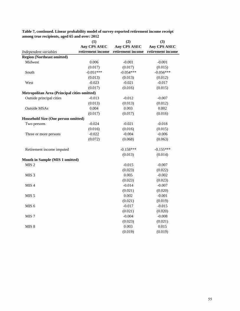
(1) (2) (3)

Independent variablesAny CPS ASEC

retirement incomeAny CPS ASEC

retirement incomeAny CPS ASEC

retirement incomeRegion (Northeast omitted)

Midwest 0.006 -0.001 -0.001(0.017) (0.017) (0.015)

South -0.051*** -0.054*** -0.056***(0.013) (0.013) (0.012)

West -0.023 -0.021 -0.017(0.017) (0.016) (0.015)

Metropolitan Area (Principal cities omitted)Outside principal cities -0.013 -0.012 -0.007

(0.013) (0.013) (0.012)Outside MSAs 0.004 0.003 0.002

(0.017) (0.017) (0.016)Household Size (One person omitted)

Two persons -0.024 -0.021 -0.018(0.016) (0.016) (0.015)

Three or more persons -0.022 -0.004 -0.006(0.072) (0.068) (0.063)

Retirement income imputed -0.158*** -0.155***(0.013) (0.014)

Month in Sample (MIS 1 omitted)MIS 2 -0.015 -0.007

(0.023) (0.022)MIS 3 0.005 -0.002

(0.023) (0.023)MIS 4 -0.014 -0.007

(0.021) (0.020)MIS 5 0.002 -0.001

(0.021) (0.019)MIS 6 -0.017 -0.015

(0.021) (0.020)MIS 7 -0.004 -0.008

(0.023) (0.021)MIS 8 0.003 0.015

(0.019) (0.019)

Table 7, continued. Linear probability model of survey-reported retirement income receipt among true recipients, aged 65 and over: 2012

55

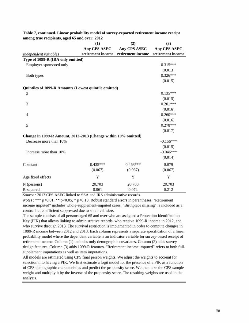
(1) (2) (3)

Independent variablesAny CPS ASEC

retirement incomeAny CPS ASEC

retirement incomeAny CPS ASEC

retirement incomeType of 1099-R (IRA only omitted)

Employer-sponsored only 0.315***(0.013)

Both types 0.326***(0.015)

Quintiles of 1099-R Amounts (Lowest quintile omitted)2 0.135***

(0.015)3 0.201***

(0.016)4 0.260***

(0.016)5 0.278***

(0.017)Change in 1099-R Amount, 2012-2013 (Change within 10% omitted)

Decrease more than 10% -0.156***(0.015)

Increase more than 10% -0.046***(0.014)

Constant 0.435*** 0.463*** 0.079(0.067) (0.067) (0.067)

Age fixed effects Y Y Y

N (persons) 20,703 20,703 20,703R-squared 0.061 0.074 0.212Source : 2013 CPS ASEC linked to SSA and IRS administrative records.Notes : *** p<0.01, ** p<0.05, * p<0.10. Robust standard errors in parentheses. "Retirement income imputed" includes whole-supplement-imputed cases. "Birthplace missing" is included as a control but coefficient suppressed due to small cell size. The sample consists of all persons aged 65 and over who are assigned a Protection Identification Key (PIK) that allows linking to administrative records, who receive 1099-R income in 2012, and who survive through 2013. The survival restriction is implemented in order to compute changes in 1099-R income between 2012 and 2013. Each column represents a separate specification of a linear probability model where the dependent variable is an indicator variable for survey-based receipt of retirement income. Column (1) includes only demographic covariates. Column (2) adds survey design features. Column (3) adds 1099-R features. “Retirement income imputed” refers to both full-supplement imputations as well as item imputations. All models are estimated using CPS final person weights. We adjust the weights to account for selection into having a PIK. We first estimate a logit model for the presence of a PIK as a function of CPS demographic characteristics and predict the propensity score. We then take the CPS sample weight and multiply it by the inverse of the propensity score. The resulting weights are used in the analysis.

Table 7, continued. Linear probability model of survey-reported retirement income receipt among true recipients, aged 65 and over: 2012

56

Table 8. Receipt rates and amounts of retirement income and Social Security across Aged Unit income distribution: 2012

Panel A: Retirement income

CPS CPS CPS

Total Total D.B. IRANon-IRA

D.C. Unknown Total Total D.B. IRANon-IRA

D.C. Unknown Total Total D.B. IRANon-IRA

D.C. Unknown

1 5,032 0.07 0.36 0.29 0.12 0.03 0.02 216 6,177 4,704 1,143 162 165 3,109 17,202 16,003 9,598 6,245 9,4362 11,620 0.12 0.41 0.35 0.15 0.02 0.02 467 4,812 3,643 1,020 82 66 3,903 11,810 10,554 6,915 4,725 4,2073 15,381 0.22 0.57 0.46 0.22 0.02 0.02 966 8,685 6,108 2,203 223 148 4,455 15,249 13,371 10,007 10,689 7,4484 19,604 0.35 0.66 0.52 0.30 0.03 0.02 2,058 13,617 10,169 3,151 157 140 5,852 20,610 19,474 10,617 5,676 5,7355 25,075 0.47 0.76 0.63 0.35 0.04 0.04 3,933 16,335 9,559 6,062 326 388 8,340 21,410 15,274 17,413 7,402 10,8636 31,757 0.59 0.81 0.68 0.39 0.06 0.03 7,046 20,027 12,328 6,724 484 491 11,914 24,631 18,092 17,300 8,692 14,6517 40,793 0.65 0.84 0.71 0.43 0.07 0.05 10,601 21,357 14,193 5,971 542 647 16,276 25,569 19,904 14,039 8,297 13,7278 54,286 0.68 0.81 0.69 0.37 0.06 0.04 15,290 24,745 17,225 5,824 1,076 575 22,376 30,587 25,074 15,627 17,341 14,0379 76,677 0.66 0.80 0.68 0.41 0.08 0.04 21,446 28,998 19,774 7,119 1,264 778 32,328 36,189 29,231 17,173 14,951 20,53910 172,800 0.60 0.78 0.63 0.44 0.09 0.04 26,858 42,539 24,570 14,239 1,916 1,805 45,110 54,528 39,140 32,671 20,688 43,520

Overall 45,288 0.44 0.68 0.56 0.32 0.05 0.03 8,886 18,727 12,226 5,345 623 520 20,138 27,550 21,720 16,871 12,560 16,560

CPS CPS CPS

Total Total D.B. IRANon-IRA

D.C. Unknown Total Total D.B. IRANon-IRA

D.C. Unknown Total Total D.B. IRANon-IRA

D.C. Unknown

1 6,447 0.12 0.09 0.07 0.01 -- -- 1,280 261 235 22 -- -- 10,400 3,006 3,202 1,545 -- --2 13,046 0.21 0.28 0.22 0.06 -- 0.02 2,298 840 686 120 -- 32 10,960 2,977 3,129 1,955 -- 1,7463 18,841 0.32 0.56 0.45 0.15 0.02 0.02 3,388 2,606 2,120 363 51 69 10,479 4,666 4,703 2,495 2,932 2,9274 25,171 0.42 0.73 0.60 0.24 0.02 0.03 4,428 5,618 4,452 905 77 179 10,643 7,734 7,467 3,710 3,219 7,0745 32,505 0.48 0.82 0.65 0.36 0.04 0.04 6,191 9,458 7,183 1,828 136 309 12,917 11,581 11,095 5,103 3,620 7,6406 41,819 0.56 0.87 0.73 0.37 0.05 0.04 8,821 14,543 11,442 2,470 267 334 15,805 16,754 15,572 6,697 5,271 9,1367 52,646 0.55 0.87 0.73 0.44 0.06 0.04 10,331 18,734 13,948 3,833 423 479 18,645 21,555 19,154 8,765 7,108 12,2998 67,436 0.61 0.87 0.75 0.49 0.09 0.04 14,407 27,146 19,901 5,986 557 696 23,502 31,067 26,607 12,292 6,433 15,7079 92,249 0.60 0.87 0.75 0.52 0.10 0.03 17,213 37,265 25,677 9,788 1,269 520 28,674 42,606 34,023 18,957 12,536 17,88210 230,579 0.54 0.84 0.68 0.54 0.11 0.06 20,507 70,818 36,625 28,139 3,448 2,583 38,280 84,149 54,177 52,534 30,554 46,712

Overall 58,068 0.44 0.68 0.56 0.32 0.05 0.03 8,886 18,727 12,226 5,345 623 520 20,138 27,550 21,720 16,871 12,560 16,560

Weighted count (Aged Units)N (Aged Units)

Admin Admin

Retirement Income

Mean Amount (Unconditional)

Mean Amount(Conditional on Receipt)

Admin Admin

16,053

Mean CPS Aged Unit Income

CPS Aged Unit Income Decile

Mean Amount(Conditional on Receipt)

Admin

Mean Amount (Unconditional)Receipt

Admin Aged Unit Income Decile

Mean Admin Aged Unit Income

32,613,260

Admin

Receipt

57

Panel B: Social Security

CPS Admin CPS Admin CPS Admin

1 5,032 0.56 0.72 3,815 9,043 6,794 12,5962 11,620 0.94 0.87 10,129 10,745 10,829 12,3253 15,381 0.95 0.92 13,212 13,431 13,950 14,6384 19,604 0.94 0.93 15,547 15,242 16,457 16,4415 25,075 0.95 0.93 18,012 18,012 18,886 19,3136 31,757 0.92 0.93 18,857 19,261 20,475 20,6747 40,793 0.92 0.93 20,670 20,450 22,517 22,0658 54,286 0.89 0.90 21,456 20,539 24,205 22,7529 76,677 0.87 0.89 20,577 20,631 23,591 23,23510 172,800 0.79 0.85 20,349 21,512 25,602 25,309

Overall 45,288 0.87 0.89 16,254 16,884 18,617 19,046

CPS Admin CPS Admin CPS Admin

1 6,447 0.75 0.54 8,159 3,892 10,930 7,1772 13,046 0.89 0.94 11,516 10,850 12,977 11,6013 18,841 0.92 0.96 14,046 14,450 15,286 15,1064 25,171 0.92 0.95 15,124 15,926 16,519 16,7355 32,505 0.91 0.93 16,553 17,232 18,184 18,5536 41,819 0.90 0.93 17,784 19,115 19,666 20,6097 52,646 0.90 0.93 19,160 20,569 21,331 22,1408 67,436 0.90 0.93 20,112 21,436 22,459 23,0219 92,249 0.87 0.90 20,605 22,303 23,571 24,68110 230,579 0.78 0.86 19,491 23,068 24,972 26,865

Overall 58,068 0.87 0.89 16,254 16,884 18,617 19,046

Weighted count (Aged Units)N (Aged Units)

Social Security

ReceiptMean Amount

(Unconditional) Mean Amount

(Conditional on Receipt)

Receipt Mean Amount (Unconditional)

Mean Amount (Conditional on Receipt)

Source : 2013 CPS ASEC linked to SSA and IRS administrative records.Notes : The sample consists of aged units as defined in the Social Security Administration’s Income of the Aged Chartbook, 2012 . Aged units are either unmarried individuals aged 65 and over or married couples where the husband is aged 65 and over (or married couples where the wife is aged 65 and over and the husband is less than 55). For married couples, incomes of both spouses are combined. Each aged unit is one observation in our analysis. We restrict attention to aged units where the unit head is assigned a Protection Identification Key (PIK) that allows linking to administrative records. Panel A reports retirement income receipt rates, unconditional mean, and conditional mean amounts using both the survey and the administrative record measures. Retirement income includes retirement, survivor, and disability pensions (excluding Social Security) as well as defined contribution account withdrawals. The top half of Panel A ranks aged units by total survey income deciles while the bottom half ranks aged units by total administrative record income deciles. Total administrative record retirement income from the 1099-R is further categorized as defined benefit, IRA, non-IRA defined contribution, and unknown. For further details about how these categories are determined, please see the Method Appendix. Panel B reports Social Security receipt rates, unconditional mean and conditional mean amounts using both the survey and the administrative record measures. The top half of Panel B ranks aged units by total survey income deciles while the bottom half ranks aged units by total administrative record income deciles.All estimates make use of CPS final person weights for the aged unit head. We adjust the weights to account for selection into having a PIK. We first estimate a logit model for the presence of a PIK as a function of CPS demographic characteristics and predict the propensity score. We then take the CPS sample weight and multiply it by the inverse of the propensity score. The resulting weights are used in the analysis.

CPS Aged Unit Income Decile

Mean CPS Aged Unit Income

Mean Admin Aged Unit Income

Admin Aged Unit Income Decile

32,613,260 16,053

58

Total D.B. IRANon-IRA

D.C. Unknown1 6,630 0.05 0.69 0.13 0.06 0.05 -- -- -- -- 0.022 11,620 0.03 0.87 0.05 0.01 0.04 -- -- -- -- 0.013 15,381 0.03 0.86 0.02 0.02 0.06 -- -- -- -- 0.014 19,604 0.05 0.79 0.01 0.02 0.10 -- -- -- -- 0.025 25,075 0.08 0.72 0.00 0.03 0.16 -- -- -- -- 0.016 31,757 0.12 0.60 0.00 0.04 0.22 -- -- -- -- 0.027 40,793 0.16 0.51 0.00 0.04 0.26 -- -- -- -- 0.028 54,286 0.23 0.40 0.00 0.06 0.28 -- -- -- -- 0.039 76,677 0.33 0.27 0.00 0.08 0.28 -- -- -- -- 0.0310 172,800 0.47 0.15 0.00 0.14 0.19 -- -- -- -- 0.05

Overall 46,418 0.16 0.58 0.02 0.05 0.17 -- -- -- -- 0.02

N (Aged Units)

Total D.B. IRANon-IRA

D.C. Unknown1 7,518 0.03 0.55 0.30 0.04 0.06 0.05 0.00 0.00 0.00 0.022 13,046 0.03 0.83 0.04 0.02 0.06 0.05 0.01 0.00 0.00 0.013 18,841 0.04 0.77 0.02 0.02 0.13 0.11 0.02 0.00 0.00 0.014 25,171 0.08 0.64 0.00 0.04 0.22 0.18 0.03 0.00 0.01 0.025 32,505 0.11 0.53 0.00 0.05 0.29 0.22 0.06 0.00 0.01 0.026 41,819 0.13 0.46 0.00 0.05 0.35 0.27 0.06 0.01 0.01 0.027 52,646 0.17 0.39 0.00 0.06 0.36 0.27 0.07 0.01 0.01 0.028 67,436 0.19 0.32 0.00 0.07 0.40 0.30 0.09 0.01 0.01 0.029 92,249 0.25 0.24 0.00 0.08 0.40 0.28 0.11 0.01 0.01 0.0210 230,579 0.35 0.14 0.00 0.12 0.34 0.20 0.12 0.02 0.01 0.04

Overall 58,908 0.14 0.49 0.03 0.06 0.27 0.19 0.06 0.01 0.01 0.02

Weighted (Aged Units)N (Aged Units)Source : 2013 CPS ASEC linked to SSA and IRS administrative records.Notes : The sample consists of aged units as defined in the Social Security Administration’s Income of the Aged Chartbook, 2012 . Aged units are either unmarried individuals aged 65 and over or married couples where the husband is aged 65 and over (or married couples where the wife is aged 65 and over and the husband is less than 55). For married couples, incomes of both spouses are combined. Each aged unit is one observation in our analysis. We restrict attention to aged units where the unit head is assigned a Protection Identification Key (PIK) that allows linking to administrative records. Panel A sorts aged units by total survey income into deciles and within each decile computes the average share of each income source based on survey values. Panel B repeats the analysis but uses the administrative record income to sort aged units into deciles and compute average shares of each income source. Retirement income includes retirement, survivor, and disability pensions (excluding Social Security) as well as defined contribution account withdrawals. When using the administrative records, retirement income is further categorized as defined benefit, IRA, non-IRA defined contribution, and unknown. For further details about how these categories are determined, please see the Method Appendix. Other income refers to other survey income sources outside of earnings, Social Security, SSI, interest and dividends, and retirement income. All estimates make use of CPS final person weights for the aged unit head. We adjust the weights to account for selection into having a PIK. We first estimate a logit model for the presence of a PIK as a function of CPS demographic characteristics and predict the propensity score. We then take the CPS sample weight and multiply it by the inverse of the propensity score. The resulting weights are used in the analysis.

Table 9. Average shares of income from various income sources across Aged Unit income distribution: 2012

32,613,260

EarningsSocial

Security SSIInterest and Dividends

Panel A: CPS income shares

Panel B: Admin income shares

Mean CPS

Income

Mean Admin Income

Other Income

Other Income

Interest and DividendsEarnings

15,812

Admin Aged Unit Income Decile

CPS Aged Unit Income Decile

Retirement Income

Retirement Income

SSISocial

Security

15,654

59

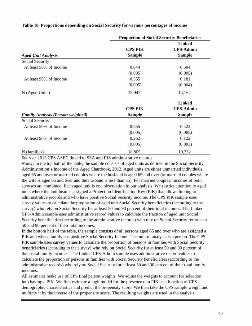
Aged Unit AnalysisCPS PIK Sample

Linked CPS-Admin

SampleSocial Security At least 50% of Income 0.644 0.504

(0.005) (0.005) At least 90% of Income 0.355 0.181

(0.005) (0.004)

N (Aged Units) 13,947 14,162

Family Analysis (Person-weighted)CPS PIK Sample

Linked CPS-Admin

SampleSocial Security At least 50% of Income 0.555 0.422

(0.005) (0.005) At least 90% of Income 0.262 0.122

(0.005) (0.003)

N (families) 18,805 19,232

Proportion of Social Security Beneficiaries

Source : 2013 CPS ASEC linked to SSA and IRS administrative records.Notes : In the top half of the table, the sample consists of aged units as defined in the Social Security Administration’s Income of the Aged Chartbook, 2012. Aged units are either unmarried individuals aged 65 and over or married couples where the husband is aged 65 and over (or married couples where the wife is aged 65 and over and the husband is less than 55). For married couples, incomes of both spouses are combined. Each aged unit is one observation in our analysis. We restrict attention to aged units where the unit head is assigned a Protection Identification Key (PIK) that allows linking to administrative records and who have positive Social Security income. The CPS PIK sample uses survey values to calculate the proportion of aged unit Social Security beneficiaries (according to the survey) who rely on Social Security for at least 50 and 90 percent of their total incomes. The Linked CPS-Admin sample uses administrative record values to calculate the fraction of aged unit Social Security beneficiaries (according to the administrative records) who rely on Social Security for at least 50 and 90 percent of their total incomes. In the bottom half of the table, the sample consists of all persons aged 65 and over who are assigned a PIK and whose family has positive Social Security Income. The unit of analysis is a person. The CPS PIK sample uses survey values to calculate the proportion of persons in families with Social Security beneficiaries (according to the survey) who rely on Social Security for at least 50 and 90 percent of their total family incomes. The Linked CPS-Admin sample uses administrative record values to calculate the proportion of persons in families with Social Security beneficiaries (according to the administrative records) who rely on Social Security for at least 50 and 90 percent of their total family incomes. All estimates make use of CPS final person weights. We adjust the weights to account for selection into having a PIK. We first estimate a logit model for the presence of a PIK as a function of CPS demographic characteristics and predict the propensity score. We then take the CPS sample weight and multiply it by the inverse of the propensity score. The resulting weights are used in the analysis.

Table 10. Proportions depending on Social Security for various percentages of income

60

(Numbers in thousands.)

Number Rate Number Rate Number Rate Number Rate Number Rate Number RateAged 65 and over 19,184 0.444 3,879 0.090 15,305 0.354 13,317 0.308 2,992 0.069 10,325 0.239Aged 65 to 74 8,866 0.359 1,937 0.079 6,929 0.280 6,377 0.258 1,665 0.067 4,712 0.191Aged 75 to 84 7,202 0.542 1,302 0.098 5,900 0.444 4,767 0.359 924 0.070 3,843 0.289Aged 85 and over 3,116 0.591 640 0.121 2,476 0.470 2,173 0.412 403 0.076 1,770 0.336

Number Rate Number Rate Number Rate Number Rate Number Rate Number RateAged 65 and over 4,191 0.097 3,879 0.090 312 0.007 3,325 0.077 2,992 0.069 333 0.008Aged 65 to 74 2,099 0.085 1,937 0.079 162 0.006 1,817 0.074 1,665 0.067 152 0.007Aged 75 to 84 1,405 0.106 1,302 0.098 103 0.008 1,058 0.080 924 0.070 134 0.010Aged 85 and over 688 0.130 640 0.121 48 0.009 450 0.085 403 0.076 47 0.009

Number Rate Number Rate Number Rate Number Rate Number Rate Number RateAged 65 and over 5,790 0.134 3,879 0.090 1,911 0.044 5,090 0.118 2,992 0.069 2,098 0.049Aged 65 to 74 2,867 0.116 1,937 0.079 930 0.037 2,671 0.108 1,665 0.067 1,006 0.041Aged 75 to 84 1,981 0.149 1,302 0.098 679 0.051 1,735 0.131 924 0.070 811 0.061Aged 85 and over 943 0.179 640 0.121 303 0.058 685 0.130 403 0.076 282 0.054

Number Rate Number Rate Number Rate Number Rate Number Rate Number RateAged 65 and over 8,786 0.203 3,879 0.090 4,907 0.113 6,631 0.153 2,992 0.069 3,639 0.084Aged 65 to 74 5,569 0.226 1,937 0.079 3,632 0.147 4,410 0.179 1,665 0.067 2,745 0.112Aged 75 to 84 2,232 0.168 1,302 0.098 930 0.070 1,595 0.120 924 0.070 671 0.050Aged 85 and over 985 0.187 640 0.121 345 0.066 626 0.119 403 0.076 223 0.043

Number Rate Number Rate Number Rate Number Rate Number Rate Number RateAged 65 and over 4,141 0.096 3,879 0.090 262 0.006 3,278 0.076 2,992 0.069 286 0.007Aged 65 to 74 2,075 0.084 1,937 0.079 138 0.005 1,823 0.074 1,665 0.067 158 0.007Aged 75 to 84 1,373 0.103 1,302 0.098 71 0.005 1,003 0.076 924 0.070 79 0.006Aged 85 and over 693 0.132 640 0.121 53 0.011 451 0.086 403 0.076 48 0.010

N (persons)

Linked CPS-Admin Sample

Linked CPS-Admin Sample

CPS PIK Sample

CPS PIK Sample

CPS PIK Sample

Lifted out of Poverty (Difference)

Lifted out of Poverty (Difference)

Linked CPS-Admin Sample

Table 11. Number and proportion of people lifted out of poverty by income source: 2012

SSI Excluded SSI Included

Source : 2013 CPS ASEC linked to SSA and IRS administrative records. Notes : CPS PIK Sample consists of all CPS persons aged 65 and over who are assigned a Personal Identification Key (PIK) that allows linking to administrative records, but uses only survey-based income values. Linked CPS-Admin Sample is the same set of people as the CPS PIK Sample except administrative record values have replaced the survey values for five types of income: earnings, Social Security, SSI, interest and dividends, and retirement income. Retirement income includes retirement, survivor, and disability pensions (excluding Social Security) as well as defined contribution account withdrawals. All poverty calculations with the income source “included” compare total family (or unrelated individual) income to the relevant poverty threshold which varies based on the size of the family. A person is classified as in poverty if total family income is below the threshold. Poverty is recalculated with a given income source “excluded” from total family income. The difference between the two poverty calculations results in the number and proportion of people lifted out of poverty by that income source. For more details see DeNavas-Walt et al. (2013). All estimates make use of CPS final person weights. We adjust the weights to account for selection into having a PIK. We first estimate a logit model for the presence of a PIK as a function of CPS demographic characteristics and predict the propensity score. We then take the CPS sample weight and multiply it by the inverse of the propensity score. The resulting weights are used in the analysis.

Social Security Excluded

Social Security Included

Social Security Excluded

Social Security Included

Retirement Income Excluded

Retirement Income Included

Retirement Income Excluded

Retirement Income Included

Interest & Dividends Excluded

Interest & Dividends Included

Interest & Dividends Excluded

Interest & Dividends Included

CPS PIK Sample Linked CPS-Admin Sample

Lifted out of Poverty (Difference)

21,239

Lifted out of Poverty (Difference)

Lifted out of Poverty (Difference)

Lifted out of Poverty (Difference)

Lifted out of Poverty (Difference)

Lifted out of Poverty (Difference)

SSI IncludedSSI Excluded

CPS PIK Sample Linked CPS-Admin SampleEarnings Excluded Earnings Included

Lifted out of Poverty (Difference)

Earnings Excluded Earnings Included

Lifted out of Poverty (Difference)

61

Table 12. Income quartiles and poverty by years from initial Social Security claiming

Panel A: All people

CPS Admin CPS Admin CPS Admin CPS Admin CPS Admin CPS Admin

Long-Run Average Earnings

5 years before claiming -- 21,248 -- 37,244 -- 56,242 -- -- -- -- -- --10 -- 25,130 -- 42,091 -- 63,871 -- -- -- -- -- --15 -- 28,402 -- 45,209 -- 66,949 -- -- -- -- -- --20 -- 30,127 -- 46,555 -- 66,378 -- -- -- -- -- --25 -- 32,298 -- 46,993 -- 64,149 -- -- -- -- -- --

Year from Social Security Claim

t-5 29,812 31,101 51,218 53,287 81,847 83,545 0.067 0.055 0.146 0.134 0.277 0.262t-4 29,000 30,557 49,175 50,924 78,449 81,302 0.061 0.062 0.159 0.147 0.284 0.268t-3 27,437 30,247 48,897 51,043 77,147 79,718 0.076 0.064 0.165 0.155 0.304 0.283t-2 26,248 29,807 45,459 50,139 75,692 80,553 0.075 0.057 0.183 0.151 0.319 0.279t-1 24,117 27,906 42,508 46,997 69,203 73,841 0.085 0.071 0.208 0.167 0.353 0.298t 22,396 29,631 41,518 48,143 67,658 75,388 0.076 0.056 0.211 0.149 0.366 0.270t+1 21,613 27,987 38,116 45,982 64,344 71,898 0.078 0.044 0.223 0.150 0.388 0.283t+2 20,246 28,213 35,205 44,972 59,942 69,934 0.078 0.045 0.247 0.143 0.425 0.287t+3 20,665 27,687 34,891 44,888 58,631 68,638 0.066 0.041 0.229 0.150 0.414 0.290t+4 20,674 26,490 33,267 42,741 56,278 64,571 0.063 0.038 0.232 0.158 0.438 0.303t+5 20,105 26,533 33,443 42,334 54,904 64,346 0.049 0.036 0.244 0.157 0.442 0.305

Share Below 100% Poverty

Share Below 200% Poverty

Share Below 300% Poverty25th Percentile 75th Percentile

Total IncomeMedian

62

Panel B: Women

CPS Admin CPS Admin CPS Admin CPS Admin CPS Admin CPS Admin

Long-Run Average Earnings

5 years before claiming -- 19,641 -- 32,412 -- 46,244 -- -- -- -- -- --10 -- 21,561 -- 39,086 -- 54,192 -- -- -- -- -- --15 -- 23,854 -- 40,992 -- 58,261 -- -- -- -- -- --20 -- 25,349 -- 41,613 -- 58,915 -- -- -- -- -- --25 -- 26,044 -- 41,928 -- 57,562 -- -- -- -- -- --

Year from Social Security Claim

t-5 25,500 28,842 45,870 47,766 72,233 75,423 0.074 0.053 0.179 0.142 0.325 0.286t-4 26,855 28,259 45,527 47,420 71,398 76,778 0.058 0.065 0.170 0.160 0.307 0.293t-3 25,255 28,187 44,359 47,579 70,551 76,440 0.084 0.062 0.185 0.163 0.337 0.307t-2 23,321 27,288 40,800 45,760 67,867 73,692 0.081 0.058 0.211 0.166 0.366 0.307t-1 22,034 26,242 38,780 44,895 62,210 69,033 0.094 0.073 0.225 0.178 0.390 0.314t 20,068 28,050 38,462 45,312 61,727 70,629 0.082 0.061 0.236 0.161 0.397 0.284t+1 20,658 26,599 35,633 44,825 59,299 68,995 0.076 0.049 0.231 0.165 0.408 0.294t+2 18,863 26,554 33,326 42,915 54,057 64,971 0.087 0.047 0.270 0.154 0.454 0.312t+3 19,244 25,733 31,674 41,240 53,537 63,056 0.071 0.042 0.251 0.167 0.458 0.328t+4 19,129 24,511 30,856 39,479 53,267 60,040 0.074 0.040 0.258 0.177 0.472 0.338t+5 18,581 24,100 29,507 39,191 50,637 60,904 0.056 0.043 0.279 0.178 0.494 0.342

Total Income Share Below 100% Poverty

Share Below 200% Poverty

Share Below 300% Poverty25th Percentile Median 75th Percentile

63

Panel C: Men

CPS Admin CPS Admin CPS Admin CPS Admin CPS Admin CPS Admin

Long-Run Average Earnings

5 years before claiming -- 26,958 -- 45,978 -- 67,205 -- -- -- -- -- --10 -- 30,638 -- 49,466 -- 73,860 -- -- -- -- -- --15 -- 33,254 -- 50,492 -- 75,614 -- -- -- -- -- --20 -- 34,207 -- 50,791 -- 74,731 -- -- -- -- -- --25 -- 37,608 -- 50,505 -- 72,164 -- -- -- -- -- --

Year from Social Security Claim

t-5 34,994 34,864 56,711 58,304 88,544 91,627 0.059 0.056 0.109 0.126 0.225 0.237t-4 32,444 33,931 54,011 55,090 87,110 87,972 0.063 0.059 0.146 0.133 0.257 0.240t-3 30,979 32,379 54,726 55,886 84,021 84,008 0.068 0.067 0.143 0.146 0.266 0.256t-2 31,120 33,239 54,239 54,674 85,314 86,541 0.067 0.057 0.151 0.134 0.264 0.246t-1 27,615 29,860 47,415 50,141 77,908 82,342 0.075 0.070 0.190 0.154 0.311 0.280t 25,042 31,501 44,676 52,022 74,222 80,452 0.070 0.051 0.184 0.135 0.331 0.254t+1 22,876 29,788 41,248 47,073 68,738 75,593 0.080 0.039 0.214 0.134 0.367 0.270t+2 22,073 30,550 38,590 47,866 66,634 74,513 0.068 0.043 0.222 0.131 0.393 0.260t+3 22,486 30,852 39,401 48,675 64,054 74,285 0.059 0.039 0.206 0.132 0.366 0.249t+4 22,079 29,434 35,956 45,811 59,980 68,593 0.050 0.036 0.203 0.138 0.401 0.265t+5 22,189 29,517 37,556 45,083 59,926 67,529 0.041 0.029 0.207 0.135 0.388 0.268Source : 1999-2013 CPS ASEC linked to SSA and IRS administrative records.Notes : We draw comparable individuals in each linked CPS-ASEC sample for our synthetic cohort analysis. Panel A shows results for the full population, panel B for women, and panel C for men. From each year of linked CPS ASEC data, we select individuals who are assigned a Protection Identification Key (PIK) that allows linking to administrative records, who, according to the administrative records, first claimed Social Security between 2003 and 2007, who were age 60 to 70 when first claiming, who did not claim disability benefits and who survived for at least five years after claiming. Individuals who first claimed in 2003 are drawn from the 1999 CPS ASEC to cover time t-5, from the 2000 CPS ASEC to cover time t-4, from the 2001 CPS ASEC to cover time t-3, etc. We pool all the claimants between 2003 and 2007 to estimate each of the eleven time periods surrounding the year Social Security is claimed. If individuals are married in a particular year we assign individuals in our sample the pooled incomes of both spouses and equivalence adjust using the Betson Scale. All income figures are inflation-adjusted using the CPI-U-RS and expressed in 2012 dollar. We report the 25th, 50th, and 75th percentiles of real, equivalized incomes in each year using both survey values and the administrative records. Long-run average earnings are calculated as the 5, 10, 15, 20, or 25 year of earnings prior to claiming. For individuals who are married, both spouses' long-run earnings are pooled and equivalence adjusted. We take the average of long-run earnings for individuals near the specified income percentile. For example, for median incomes, we average long-run earnings for individuals with income between the 45th and 55th percentile. All long-run earnings calculations are based on the t-5 sample. We calculate using both the survey and the administrative records the share of the sample below 100, 200 and 300 percent of poverty by comparing the individual’s total family (or unrelated individual) income to the relevant poverty threshold which varies based on family size. For more details on poverty calculations, see Denavas-Walt (2013). All estimates make use of CPS final person weights. We adjust the weights to account for selection into having a PIK. We first estimate a logit model for the presence of a PIK as a function of CPS demographic characteristics and predict the propensity score. We then take the CPS sample weight and multiply it by the inverse of the propensity score. The resulting weights are used in the analysis.

Total Income Share Below 100% Poverty

Share Below 200% Poverty

Share Below 300% Poverty25th Percentile Median 75th Percentile

64

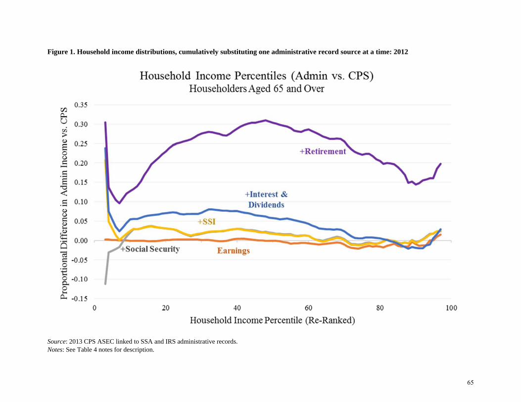
Figure 1. Household income distributions, cumulatively substituting one administrative record source at a time: 2012

Source: 2013 CPS ASEC linked to SSA and IRS administrative records. Notes: See Table 4 notes for description.

65

Figure 2. CPS ASEC retirement receipt by Form 1099-R amount percentile: 2012

Source: 2013 CPS ASEC linked to IRS Form 1099-R records. Notes: Sample consists of all persons aged 65 and over who are assigned a Protection Identification Key (PIK) that allows linking to administrative records, who have positive 1099-R income, and who have non-imputed survey responses for retirement income. Individuals are ranked based on percentile of 1099-R income (x-axis). For each percentile, the mean survey-based rate of retirement income receipt (y-axis) is calculated. Retirement income includes retirement, survivor, and disability pensions (excluding Social Security) as well as defined contribution account withdrawals. All estimates make use of CPS final person weights. We adjust the weights to account for selection into having a PIK. We first estimate a logit model for the presence of a PIK as a function of CPS demographic characteristics and predict the propensity score. We then take the CPS sample weight and multiply it by the inverse of the propensity score. The resulting weights are used in the analysis.

66

Figure 3. Historical trends in household income quartiles (2012 dollars)

Source: 1991, 1996, and 1999-2013 CPS ASEC; and 1990, 1996, 2001, 2004, and 2008 SIPP panels (Wave 1) linked to SSA and IRS administrative records. Notes: Sample consists of all householders aged 65 and over, and the two linked samples further require that householders are assigned a Protection Identification Key (PIK) that allows linking to administrative records. Each panel plots the 25th, 50th, and 75th, percentile of household incomes from both the survey (Full CPS Sample) and the administrative records (Linked CPS-Admin Sample and Linked SIPP-Admin Sample). All estimates make use of CPS or SIPP final household weights. For the linked samples, we adjust the weights to account for selection into having a PIK. We first estimate a logit model for the presence of a PIK as a function of CPS/SIPP demographic characteristics and predict the propensity score. We then take the CPS/SIPP sample weight and multiply it by the inverse of the propensity score. The resulting weights are used in the analysis.

67

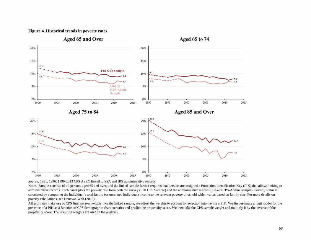
Figure 4. Historical trends in poverty rates

Source: 1991, 1996, 1999-2013 CPS ASEC linked to SSA and IRS administrative records. Notes: Sample consists of all persons aged 65 and over, and the linked sample further requires that persons are assigned a Protection Identification Key (PIK) that allows linking to administrative records. Each panel plots the poverty rate from both the survey (Full CPS Sample) and the administrative records (Linked CPS-Admin Sample). Poverty status is calculated by comparing the individual’s total family (or unrelated individual) income to the relevant poverty threshold which varies based on family size. For more details on poverty calculations, see Denavas-Walt (2013). All estimates make use of CPS final person weights. For the linked sample, we adjust the weights to account for selection into having a PIK. We first estimate a logit model for the presence of a PIK as a function of CPS demographic characteristics and predict the propensity score. We then take the CPS sample weight and multiply it by the inverse of the propensity score. The resulting weights are used in the analysis.

68

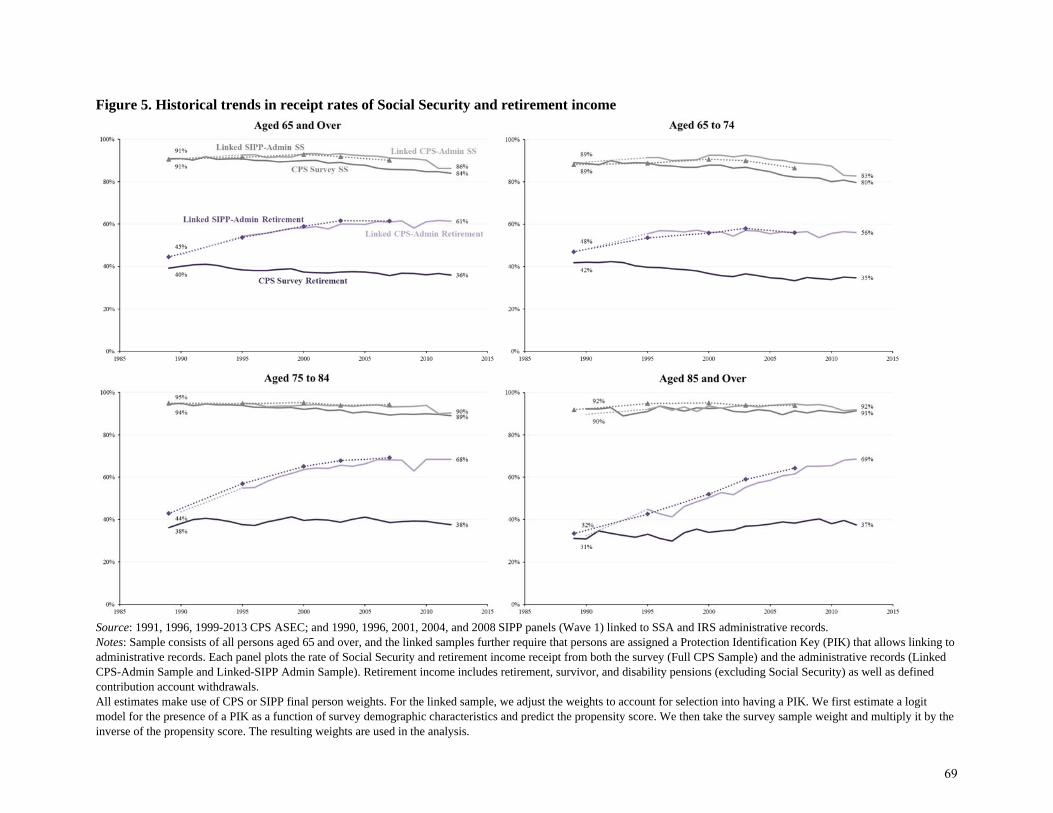
Figure 5. Historical trends in receipt rates of Social Security and retirement income

Source: 1991, 1996, 1999-2013 CPS ASEC; and 1990, 1996, 2001, 2004, and 2008 SIPP panels (Wave 1) linked to SSA and IRS administrative records. Notes: Sample consists of all persons aged 65 and over, and the linked samples further require that persons are assigned a Protection Identification Key (PIK) that allows linking to administrative records. Each panel plots the rate of Social Security and retirement income receipt from both the survey (Full CPS Sample) and the administrative records (Linked CPS-Admin Sample and Linked-SIPP Admin Sample). Retirement income includes retirement, survivor, and disability pensions (excluding Social Security) as well as defined contribution account withdrawals. All estimates make use of CPS or SIPP final person weights. For the linked sample, we adjust the weights to account for selection into having a PIK. We first estimate a logit model for the presence of a PIK as a function of survey demographic characteristics and predict the propensity score. We then take the survey sample weight and multiply it by the inverse of the propensity score. The resulting weights are used in the analysis.

69

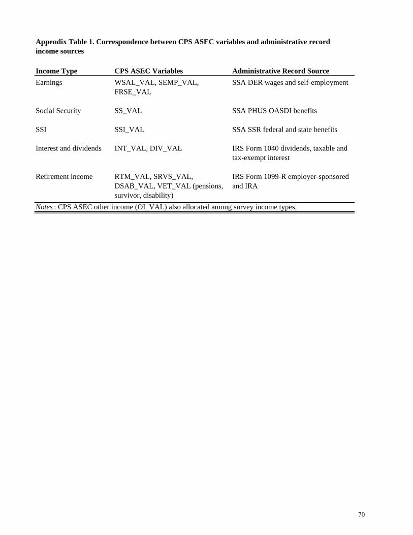
Income Type CPS ASEC Variables Administrative Record Source

Earnings WSAL_VAL, SEMP_VAL, FRSE_VAL

SSA DER wages and self-employment

Social Security SS_VAL SSA PHUS OASDI benefits

SSI SSI_VAL SSA SSR federal and state benefits

Interest and dividends INT_VAL, DIV_VAL IRS Form 1040 dividends, taxable and tax-exempt interest

Retirement income RTM_VAL, SRVS_VAL, DSAB_VAL, VET_VAL (pensions, survivor, disability)

IRS Form 1099-R employer-sponsored and IRA

Notes : CPS ASEC other income (OI_VAL) also allocated among survey income types.

Appendix Table 1. Correspondence between CPS ASEC variables and administrative record income sources

70

(1) (2)Independent variables Survey Median Admin Median

Disabled -3,104*** -6,558***(514) (652)

Homeowner 5,594*** 9,674***(622) (788)

Veteran 4,863*** 3,848***(783) (863)

Race and Hispanic Origin (White, not Hispanic omitted)Black, not Hispanic -3,520*** -3,126***

(717) (955)Asian, not Hispanic -1,115 -2,211

(1,602) (2,024)Other race, not Hispanic -5,435** -4,659

(2,548) (4,270)Hispanic, any race -6,059*** -6,311***

(987) (1,214)Education (Less than high school omitted)

High school graduate 3,933*** 5,260***(544) (693)

Some college 7,768*** 11,684***(675) (949)

College graduate 26,498*** 36,696***(1,439) (1,410)

Nativity (US born omitted)Foreign born -2,446*** -4,703***

(816) (1,245)Marital Status (Married omitted)

Married, spouse absent -10,061*** -13,064***(2,536) (3,034)

Widowed -5,457*** -8,356***(1,360) (1,513)

Divorced -8,572*** -12,530***(1,334) (1,529)

Separated -10,087*** -11,093***(2,539) (2,899)

Never married -9,673*** -11,679***(1,567) (1,746)

Region (Northeast omitted)Midwest -149 -2,369**

(769) (953)South -2,553*** -5,063***

(730) (886)West 23 -2,516**

(916) (1,144)

Appendix Table 2. Quantile regression of survey- and administrative-record-reported median household income, aged 65 and over: 2012

71

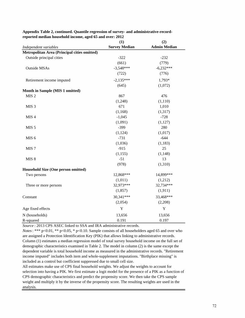
(1) (2)Independent variables Survey Median Admin MedianMetropolitan Area (Principal cities omitted)

Outside principal cities -322 -232(661) (779)

Outside MSAs -3,548*** -6,232***(722) (776)

Retirement income imputed -2,135*** 1,793*(645) (1,072)

Month in Sample (MIS 1 omitted)MIS 2 867 476

(1,248) (1,110)MIS 3 671 1,010

(1,168) (1,317)MIS 4 -1,045 -728

(1,091) (1,127)MIS 5 -399 280

(1,124) (1,017)MIS 6 -731 -644

(1,036) (1,183)MIS 7 -915 25

(1,155) (1,148)MIS 8 -51 13

(978) (1,310)Household Size (One person omitted)

Two persons 12,868*** 14,899***(1,011) (1,212)

Three or more persons 32,973*** 32,734***(1,857) (1,911)

Constant 30,341*** 33,468***(2,054) (2,208)

Age fixed effects Y YN (households) 13,656 13,656R-squared 0.191 0.197Source : 2013 CPS ASEC linked to SSA and IRA administrative records. Notes : *** p<0.01, ** p<0.05, * p<0.10. Sample consists of all householders aged 65 and over who are assigned a Protection Identification Key (PIK) that allows linking to administrative records. Column (1) estimates a median regression model of total survey household income on the full set of demographic characteristics examined in Table 2. The model in column (2) is the same except the dependent variable is total household income as measured in the administrative records. "Retirement income imputed" includes both item and whole-supplement imputations. "Birthplace missing" is included as a control but coefficient suppressed due to small cell size.All estimates make use of CPS final household weights. We adjust the weights to account for selection into having a PIK. We first estimate a logit model for the presence of a PIK as a function of CPS demographic characteristics and predict the propensity score. We then take the CPS sample weight and multiply it by the inverse of the propensity score. The resulting weights are used in the analysis.

Appendix Table 2, continued. Quantile regression of survey- and administrative-record-reported median household income, aged 65 and over: 2012

72

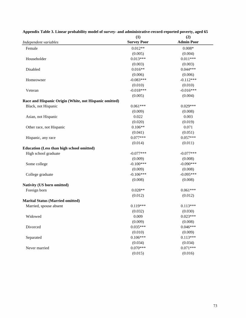
(1) (2)Independent variables Survey Poor Admin Poor

Female 0.012** 0.008*(0.005) (0.004)

Householder 0.013*** 0.011***(0.003) (0.003)

Disabled 0.016** 0.044***(0.006) (0.006)

Homeowner -0.083*** -0.112***(0.010) (0.010)

Veteran -0.018*** -0.016***(0.005) (0.004)

Race and Hispanic Origin (White, not Hispanic omitted)Black, not Hispanic 0.061*** 0.029***

(0.009) (0.008)Asian, not Hispanic 0.022 0.003

(0.020) (0.019)Other race, not Hispanic 0.106** 0.071

(0.041) (0.051)Hispanic, any race 0.077*** 0.057***

(0.014) (0.011)Education (Less than high school omitted)

High school graduate -0.077*** -0.077***(0.009) (0.008)

Some college -0.100*** -0.090***(0.009) (0.008)

College graduate -0.106*** -0.095***(0.008) (0.008)

Nativity (US born omitted)Foreign born 0.028** 0.061***

(0.012) (0.012)Marital Status (Married omitted)

Married, spouse absent 0.119*** 0.113***(0.032) (0.030)

Widowed 0.009 0.023***(0.009) (0.008)

Divorced 0.035*** 0.046***(0.010) (0.009)

Separated 0.106*** 0.113***(0.034) (0.034)

Never married 0.070*** 0.071***(0.015) (0.016)

Appendix Table 3. Linear probability model of survey- and administrative-record-reported poverty, aged 65

73

(1) (2)Independent variables Survey Poor Admin PoorRegion (Northeast omitted)

Midwest -0.008 -0.006(0.008) (0.006)

South 0.019*** 0.016**(0.007) (0.006)

West 0.001 0.004(0.007) (0.007)

Metropolitan Area (Principal cities omitted)Outside principal cities -0.018** -0.017***

(0.008) (0.007)Outside MSAs 0.001 0.018**

(0.006) (0.006)Retirement income imputed 0.008 -0.006

(0.006) (0.005)Month in Sample (MIS 1 omitted)

MIS 2 -0.016 -0.008(0.011) (0.009)

MIS 3 -0.011 -0.001(0.009) (0.008)

MIS 4 0.002 0.006(0.010) (0.009)

MIS 5 -0.016* -0.007(0.010) (0.008)

MIS 6 -0.007 -0.005(0.010) (0.010)

MIS 7 -0.007 -0.008(0.010) (0.009)

MIS 8 -0.007 0.003(0.010) (0.008)

Appendix Table 3, continued. Linear probability model of survey- and administrative-record-reported poverty, aged 65 and over: 2012

74

(1) (2)Independent variables Survey Poor Admin PoorHousehold Size (One person omitted)

Two persons -0.054*** -0.036***(0.009) (0.008)

Three or more persons -0.064*** -0.049***(0.009) (0.009)

Constant 0.258*** 0.233***(0.018) (0.017)

Age fixed effects Y YN (persons) 21,239 21,239R-squared 0.106 0.145Source : 2013 CPS ASEC linked to SSA and IRS administrative records. Notes : *** p<0.01, ** p<0.05, * p<0.10. Sample consists of all persons aged 65 and over who are assigned a Protection Identification Key (PIK) that allows linking to administrative records. Column (1) estimates a linear probability model of survey-based poverty status on the full set of demographic characteristics examined in Table 3. "Retirement income imputed" includes both item and whole-supplement imputations. "Birthplace missing" is included as a control but coefficient suppressed due to small cell size. Poverty status is determined by comparing total family (or unrelated individual) income to the relevant poverty threshold which varies by family size. A person is classified as in poverty if total family income is below the threshold. For more details see DeNavas-Walt et al. (2013). The model in column (2) is the same except the dependent variable is poverty status as measured in the administrative records.All estimates make use of CPS final person weights. We adjust the weights to account for selection into having a PIK. We first estimate a logit model for the presence of a PIK as a function of CPS demographic characteristics and predict the propensity score. We then take the CPS sample weight and multiply it by the inverse of the propensity score. The resulting weights are used in the analysis.

Appendix Table 3, continued. Linear probability model of survey- and administrative-record-reported poverty, aged 65 and over: 2012

75

1+ 1 2 3+ 1+ 1 2 3+ 1+ 1 2 3+

Aged 65 and over 0.613 0.315 0.170 0.128 0.498 0.330 0.121 0.048 0.284 0.211 0.052 0.022

Aged 65-74 0.560 0.310 0.148 0.102 0.462 0.316 0.109 0.038 0.227 0.166 0.045 0.016Aged 75-84 0.684 0.314 0.203 0.168 0.536 0.345 0.134 0.057 0.384 0.282 0.068 0.035Aged 85 and over 0.685 0.343 0.192 0.150 0.577 0.360 0.147 0.070 0.306 0.249 0.043 0.014

N (persons)

Source : 2013 CPS-ASEC linked to SSA and IRS administrative records.Notes : Sample consists of all persons aged 65 and over who are assigned a Protection Identification Key (PIK) that allows linking to administrative records. All estimates make use of CPS final person weights. We adjust the weights to account for selection into having a PIK. We first estimate a logit model for the presence of a PIK as a function of CPS demographic characteristics and predict the propensity score. We then take the CPS sample weight and multiply it by the inverse of the propensity score. The resulting weights are used in the analysis.

Appendix Table 4. Proportion of persons aged 65 and over who receive designated number of 1099-Rs in TY 2012

21,239

Number of 1099-Rs

Number of Employer-Sponsored 1099-Rs

Number of IRA 1099-Rs

76

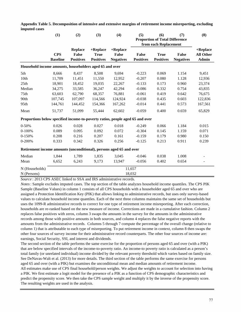
(1) (2) (3) (4) (5) (6) (7) (8)

CPS Baseline

Replace False

Positives

+Replace True

Positives

+Replace False

NegativesFalse

PositivesTrue

PositivesFalse

Negatives

+Replace All Other

Admin

Household income amounts, householders aged 65 and over

5th 8,666 8,437 8,508 9,694 -0.223 0.069 1.154 9,45110th 11,709 11,451 11,550 12,952 -0.207 0.080 1.128 12,93625th 18,901 18,452 19,035 22,267 -0.133 0.173 0.960 23,374Median 34,275 33,585 36,247 42,294 -0.086 0.332 0.754 43,83575th 63,603 62,790 68,357 76,881 -0.061 0.419 0.642 76,67590th 107,745 107,097 114,566 124,924 -0.038 0.435 0.603 122,83695th 144,761 144,452 154,366 167,262 -0.014 0.441 0.573 167,561

Mean 51,737 51,099 55,444 62,602 -0.059 0.400 0.659 65,829

Proportions below specified income-to-poverty ratios, people aged 65 and over

0-50% 0.026 0.028 0.027 0.018 -0.249 0.066 1.184 0.0150-100% 0.089 0.095 0.092 0.072 -0.304 0.145 1.159 0.0710-150% 0.208 0.216 0.207 0.161 -0.159 0.179 0.980 0.1500-200% 0.333 0.342 0.326 0.256 -0.125 0.213 0.911 0.239

Retirement income amounts (unconditional), persons aged 65 and over

Median 1,844 1,789 1,835 3,045 -0.046 0.038 1.008 -Mean 6,652 6,243 9,173 13,947 -0.056 0.402 0.654 -

N (Households)N (Persons)

Appendix Table 5. Decomposition of intensive and extensive margins of retirement income misreporting, excluding imputed cases

11,65718,032

Source : 2013 CPS ASEC linked to SSA and IRS administrative records.Notes : Sample excludes imputed cases. The top section of the table analyzes household income quantiles. The CPS PIK Sample (Baseline Values) in column 1 consists of all CPS households with a householder aged 65 and over who are assigned a Protection Identification Key (PIK) that allows linking to administrative records, but uses only survey-based values to calculate household income quantiles. Each of the next three columns maintains the same set of households but uses the 1099-R administrative records to correct for one type of retirement income misreporting. After each correction, households are re-ranked based on the new measure of income. Corrections are made in a cumulative fashion. Column 2 replaces false positives with zeros, column 3 swaps the amounts in the survey for the amounts in the administrative records among those with positive amounts in both sources, and column 4 replaces the false negative reports with the amounts from the administrative records. Columns 5 through 7 compute the percentage of the overall change (relative to column 1) that is attributable to each type of misreporting. To put retirement income in context, column 8 then swaps the other four sources of survey income for their administrative record counterparts. The other four sources of income are: earnings, Social Security, SSI, and interest and dividends. The second section of the table performs the same exercise for the proportion of persons aged 65 and over (with a PIK) that are below specified intervals of the income-to-poverty ratio. An income-to poverty ratio is calculated as a person’s total family (or unrelated individual) income divided by the relevant poverty threshold which varies based on family size. See DeNavas-Walt et al. (2013) for more details. The third section of the table performs the same exercise for persons aged 65 and over (with a PIK) but examines the unconditional mean and median amounts of retirement income. All estimates make use of CPS final household/person weights. We adjust the weights to account for selection into having a PIK. We first estimate a logit model for the presence of a PIK as a function of CPS demographic characteristics and predict the propensity score. We then take the CPS sample weight and multiply it by the inverse of the propensity score. The resulting weights are used in the analysis.

Proportion of Total Difference from each Replacement

77

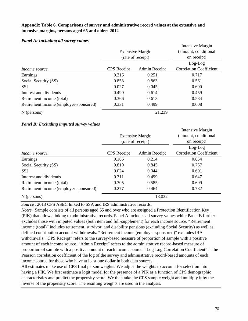
Panel A: Including all survey valuesIntensive Margin

(amount, conditional on receipt)

Income source CPS Receipt Admin ReceiptLog-Log

Correlation CoefficientEarnings 0.216 0.251 0.717Social Security (SS) 0.853 0.863 0.561SSI 0.027 0.045 0.600Interest and dividends 0.490 0.614 0.459Retirement income (total) 0.366 0.613 0.534Retirement income (employer-sponsored) 0.331 0.499 0.608

N (persons)

Panel B: Excluding imputed survey valuesIntensive Margin

(amount, conditional on receipt)

Income source CPS Receipt Admin ReceiptLog-Log

Correlation CoefficientEarnings 0.166 0.214 0.854Social Security (SS) 0.819 0.845 0.757SSI 0.024 0.044 0.691Interest and dividends 0.311 0.499 0.647Retirement income (total) 0.305 0.585 0.699Retirement income (employer-sponsored) 0.277 0.464 0.782

N (persons)

Appendix Table 6. Comparisons of survey and administrative record values at the extensive and intensive margins, persons aged 65 and older: 2012

Source : 2013 CPS ASEC linked to SSA and IRS administrative records.Notes : Sample consists of all persons aged 65 and over who are assigned a Protection Identification Key (PIK) that allows linking to administrative records. Panel A includes all survey values while Panel B further excludes those with imputed values (both item and full-supplement) for each income source. “Retirement income (total)” includes retirement, survivor, and disability pensions (excluding Social Security) as well as defined contribution account withdrawals. “Retirement income (employer-sponsored)” excludes IRA withdrawals. “CPS Receipt” refers to the survey-based measure of proportion of sample with a positive amount of each income source. “Admin Receipt” refers to the administrative record-based measure of proportion of sample with a positive amount of each income source. “Log-Log Correlation Coefficient” is the Pearson correlation coefficient of the log of the survey and administrative record-based amounts of each income source for those who have at least one dollar in both data sources. All estimates make use of CPS final person weights. We adjust the weights to account for selection into having a PIK. We first estimate a logit model for the presence of a PIK as a function of CPS demographic characteristics and predict the propensity score. We then take the CPS sample weight and multiply it by the inverse of the propensity score. The resulting weights are used in the analysis.

Extensive Margin (rate of receipt)

Extensive Margin (rate of receipt)

18,032

21,239

78

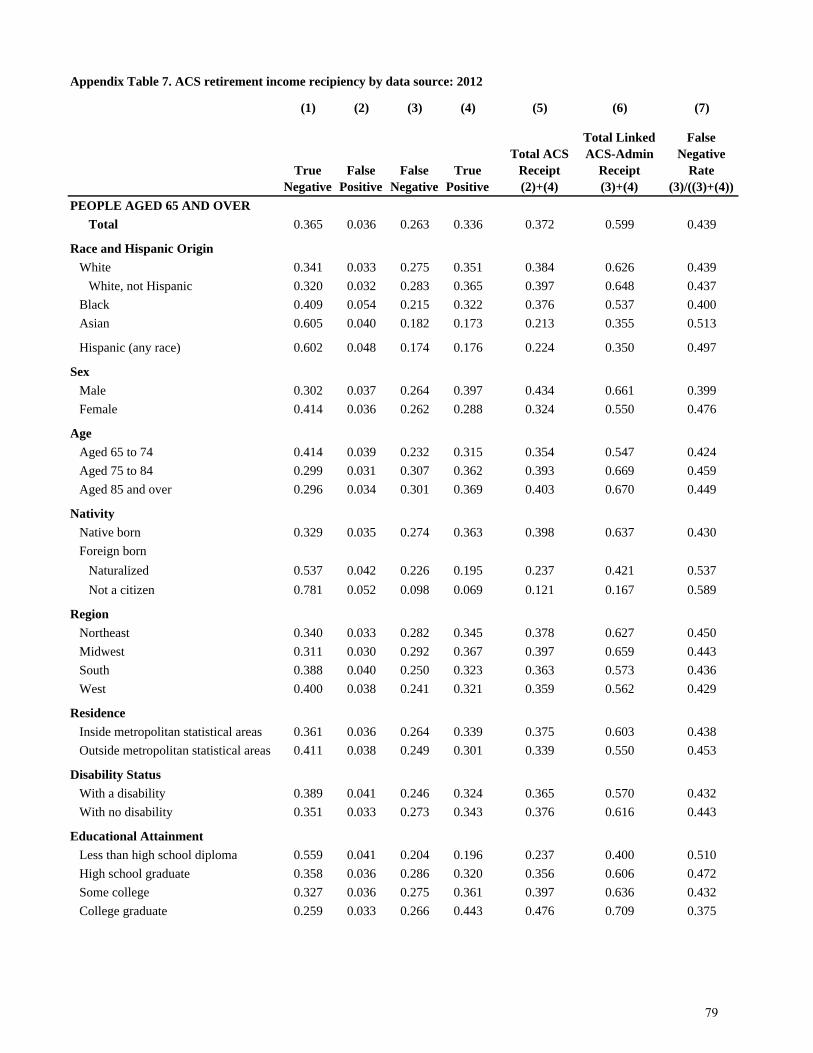
(1) (2) (3) (4) (5) (6) (7)

PEOPLE AGED 65 AND OVER

Total 0.365 0.036 0.263 0.336 0.372 0.599 0.439

Race and Hispanic Origin

White 0.341 0.033 0.275 0.351 0.384 0.626 0.439White, not Hispanic 0.320 0.032 0.283 0.365 0.397 0.648 0.437

Black 0.409 0.054 0.215 0.322 0.376 0.537 0.400Asian 0.605 0.040 0.182 0.173 0.213 0.355 0.513

Hispanic (any race) 0.602 0.048 0.174 0.176 0.224 0.350 0.497

Sex

Male 0.302 0.037 0.264 0.397 0.434 0.661 0.399Female 0.414 0.036 0.262 0.288 0.324 0.550 0.476

Age

Aged 65 to 74 0.414 0.039 0.232 0.315 0.354 0.547 0.424Aged 75 to 84 0.299 0.031 0.307 0.362 0.393 0.669 0.459Aged 85 and over 0.296 0.034 0.301 0.369 0.403 0.670 0.449

Nativity

Native born 0.329 0.035 0.274 0.363 0.398 0.637 0.430Foreign born

Naturalized 0.537 0.042 0.226 0.195 0.237 0.421 0.537Not a citizen 0.781 0.052 0.098 0.069 0.121 0.167 0.589

Region

Northeast 0.340 0.033 0.282 0.345 0.378 0.627 0.450Midwest 0.311 0.030 0.292 0.367 0.397 0.659 0.443South 0.388 0.040 0.250 0.323 0.363 0.573 0.436West 0.400 0.038 0.241 0.321 0.359 0.562 0.429

Residence

Inside metropolitan statistical areas 0.361 0.036 0.264 0.339 0.375 0.603 0.438Outside metropolitan statistical areas 0.411 0.038 0.249 0.301 0.339 0.550 0.453

Disability Status

With a disability 0.389 0.041 0.246 0.324 0.365 0.570 0.432With no disability 0.351 0.033 0.273 0.343 0.376 0.616 0.443

Educational Attainment

Less than high school diploma 0.559 0.041 0.204 0.196 0.237 0.400 0.510High school graduate 0.358 0.036 0.286 0.320 0.356 0.606 0.472Some college 0.327 0.036 0.275 0.361 0.397 0.636 0.432College graduate 0.259 0.033 0.266 0.443 0.476 0.709 0.375

Appendix Table 7. ACS retirement income recipiency by data source: 2012

Total ACS Receipt (2)+(4)

Total Linked ACS-Admin

Receipt (3)+(4)

False Negative

Rate(3)/((3)+(4))

True Negative

False Positive

False Negative

True Positive

79

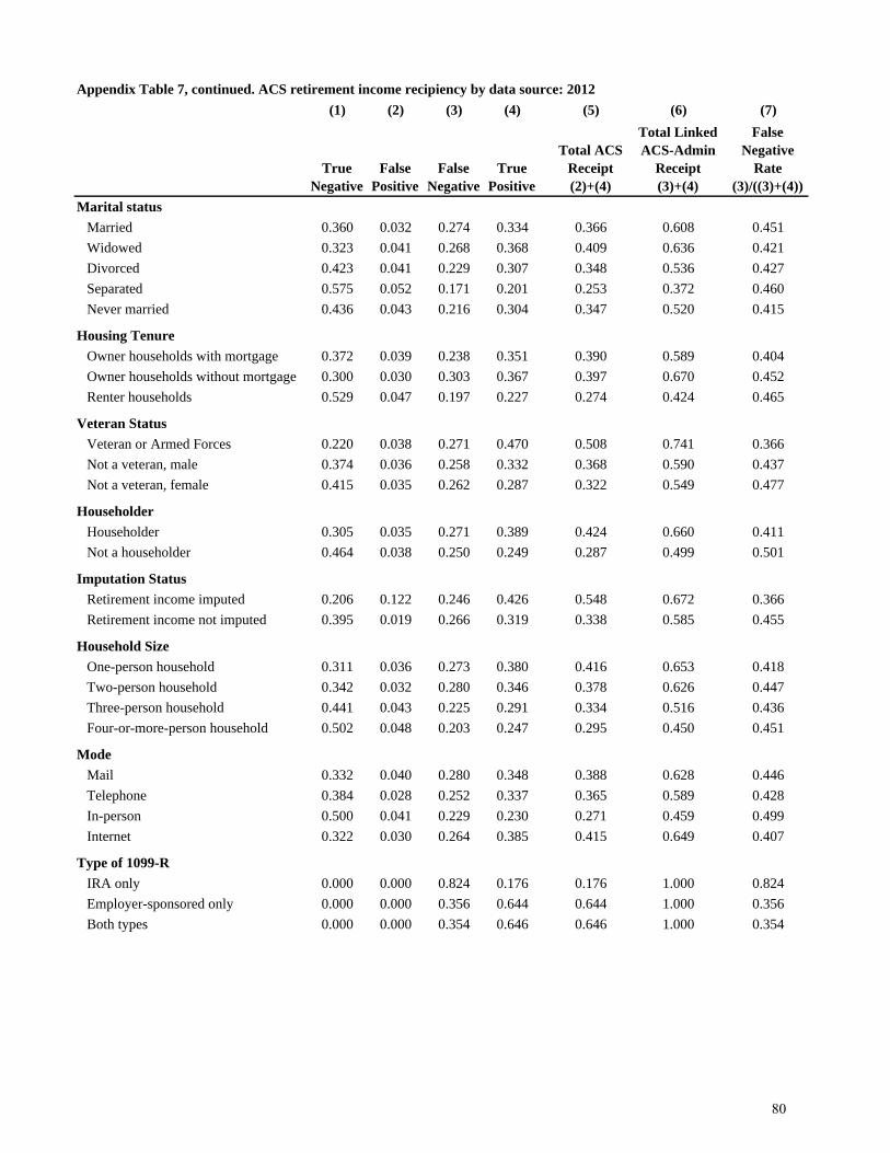
(1) (2) (3) (4) (5) (6) (7)

Marital status

Married 0.360 0.032 0.274 0.334 0.366 0.608 0.451Widowed 0.323 0.041 0.268 0.368 0.409 0.636 0.421Divorced 0.423 0.041 0.229 0.307 0.348 0.536 0.427Separated 0.575 0.052 0.171 0.201 0.253 0.372 0.460Never married 0.436 0.043 0.216 0.304 0.347 0.520 0.415

Housing Tenure

Owner households with mortgage 0.372 0.039 0.238 0.351 0.390 0.589 0.404Owner households without mortgage 0.300 0.030 0.303 0.367 0.397 0.670 0.452Renter households 0.529 0.047 0.197 0.227 0.274 0.424 0.465

Veteran Status

Veteran or Armed Forces 0.220 0.038 0.271 0.470 0.508 0.741 0.366Not a veteran, male 0.374 0.036 0.258 0.332 0.368 0.590 0.437Not a veteran, female 0.415 0.035 0.262 0.287 0.322 0.549 0.477

Householder

Householder 0.305 0.035 0.271 0.389 0.424 0.660 0.411Not a householder 0.464 0.038 0.250 0.249 0.287 0.499 0.501

Imputation Status

Retirement income imputed 0.206 0.122 0.246 0.426 0.548 0.672 0.366Retirement income not imputed 0.395 0.019 0.266 0.319 0.338 0.585 0.455

Household Size

One-person household 0.311 0.036 0.273 0.380 0.416 0.653 0.418Two-person household 0.342 0.032 0.280 0.346 0.378 0.626 0.447Three-person household 0.441 0.043 0.225 0.291 0.334 0.516 0.436Four-or-more-person household 0.502 0.048 0.203 0.247 0.295 0.450 0.451

Mode

Mail 0.332 0.040 0.280 0.348 0.388 0.628 0.446Telephone 0.384 0.028 0.252 0.337 0.365 0.589 0.428In-person 0.500 0.041 0.229 0.230 0.271 0.459 0.499Internet 0.322 0.030 0.264 0.385 0.415 0.649 0.407

Type of 1099-R

IRA only 0.000 0.000 0.824 0.176 0.176 1.000 0.824Employer-sponsored only 0.000 0.000 0.356 0.644 0.644 1.000 0.356Both types 0.000 0.000 0.354 0.646 0.646 1.000 0.354

True Negative

False Positive

False Negative

True Positive

False Negative

Rate(3)/((3)+(4))

Total ACS Receipt (2)+(4)

Total Linked ACS-Admin

Receipt (3)+(4)

Appendix Table 7, continued. ACS retirement income recipiency by data source: 2012

80

(1) (2) (3) (4) (5) (6) (7)

Quintiles of 1099-R Amounts (Conditional >0)

0.000 0.000 0.672 0.328 0.328 1.000 0.6720.000 0.000 0.505 0.495 0.495 1.000 0.5050.000 0.000 0.402 0.598 0.598 1.000 0.4020.000 0.000 0.320 0.680 0.680 1.000 0.3200.000 0.000 0.297 0.703 0.703 1.000 0.297

N (persons)Source : 2013 American Community Survey linked to 2012 IRS 1099-R records.Notes : Sample consists of all ACS persons aged 65 and over (excluding those in group quarters) who are assigned a Personal Identification Key (PIK) that allows linking to administrative records. Retirement income includes retirement, survivor, and disability pensions (excluding Social Security) as well as defined contribution account withdrawals. “True negative” refers to the proportion of the sample who have zero administrative record retirement income and report zero retirement income in the survey. “False positive” refers to the proportion of the sample with zero administrative record income but report positive income in the survey. “False negative” refers to the proportion of the sample with positive administrative record income but report zero income in the survey. “True positive” refers to the proportion of the sample with positive administrative record income and report positive income in the survey. All estimates make use of ACS final person weights. We adjust the weights to account for selection into having a PIK. We first estimate a logit model for the presence of a PIK as a function of ACS demographic characteristics and predict the propensity score. We then take the ACS sample weight and multiply it by the inverse of the propensity score. The resulting weights are used in the analysis.

819,115

Total ACS Receipt (2)+(4)

Total Linked ACS-Admin

Receipt (3)+(4)

False Negative

Rate(3)/((3)+(4))

True Negative

False Positive

False Negative

True Positive

Appendix Table 7, continued. ACS retirement income recipiency by data source: 2012

2345

1

81

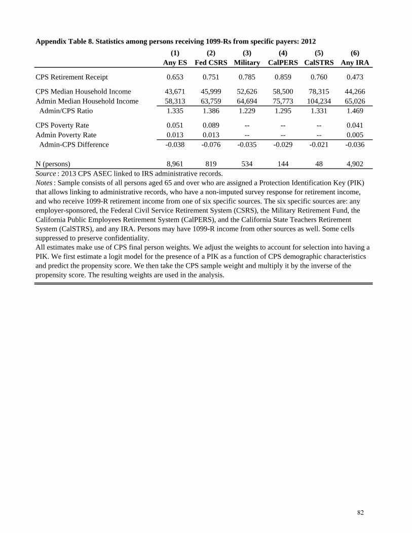
Appendix Table 8. Statistics among persons receiving 1099-Rs from specific payers: 2012

(1) (2) (3) (4) (5) (6)Any ES Fed CSRS Military CalPERS CalSTRS Any IRA

CPS Retirement Receipt 0.653 0.751 0.785 0.859 0.760 0.473

CPS Median Household Income 43,671 45,999 52,626 58,500 78,315 44,266Admin Median Household Income 58,313 63,759 64,694 75,773 104,234 65,026 Admin/CPS Ratio 1.335 1.386 1.229 1.295 1.331 1.469

CPS Poverty Rate 0.051 0.089 -- -- -- 0.041Admin Poverty Rate 0.013 0.013 -- -- -- 0.005 Admin-CPS Difference -0.038 -0.076 -0.035 -0.029 -0.021 -0.036

N (persons) 8,961 819 534 144 48 4,902Source : 2013 CPS ASEC linked to IRS administrative records.Notes : Sample consists of all persons aged 65 and over who are assigned a Protection Identification Key (PIK) that allows linking to administrative records, who have a non-imputed survey response for retirement income, and who receive 1099-R retirement income from one of six specific sources. The six specific sources are: any employer-sponsored, the Federal Civil Service Retirement System (CSRS), the Military Retirement Fund, the California Public Employees Retirement System (CalPERS), and the California State Teachers Retirement System (CalSTRS), and any IRA. Persons may have 1099-R income from other sources as well. Some cells suppressed to preserve confidentiality. All estimates make use of CPS final person weights. We adjust the weights to account for selection into having a PIK. We first estimate a logit model for the presence of a PIK as a function of CPS demographic characteristics and predict the propensity score. We then take the CPS sample weight and multiply it by the inverse of the propensity score. The resulting weights are used in the analysis.

82

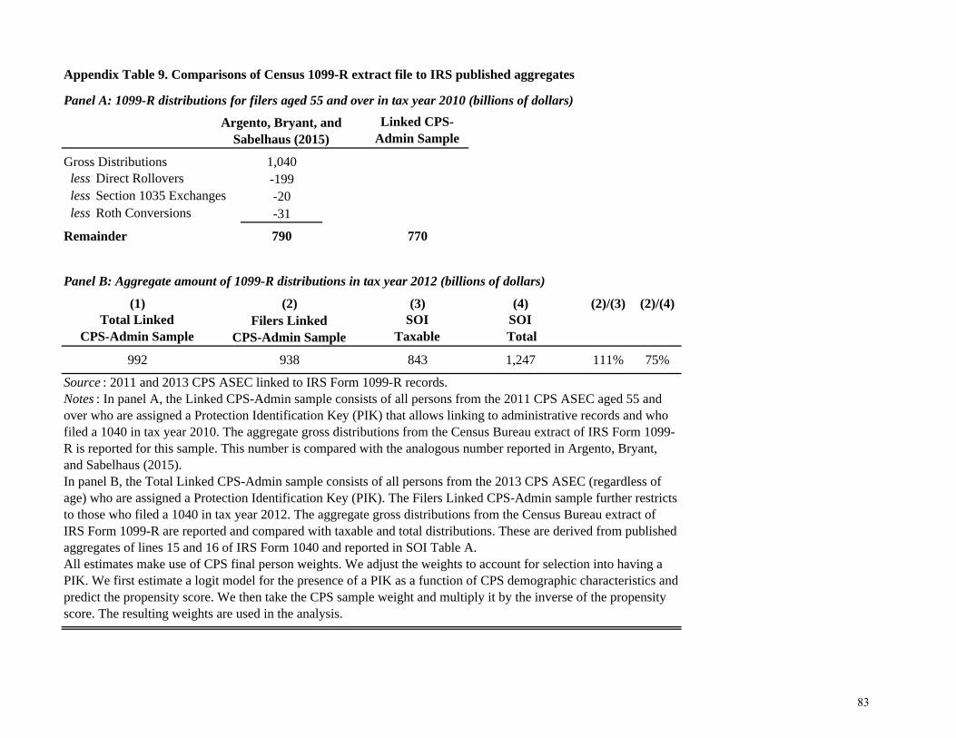
Panel A: 1099-R distributions for filers aged 55 and over in tax year 2010 (billions of dollars)

Linked CPS-Admin Sample

Gross Distributions 1,040 less Direct Rollovers -199 less Section 1035 Exchanges -20 less Roth Conversions -31

Remainder 790 770

(1) (3) (4) (2)/(3) (2)/(4)Total Linked

CPS-Admin SampleSOI

TaxableSOI

Total

992 843 1,247 111% 75%

Source : 2011 and 2013 CPS ASEC linked to IRS Form 1099-R records.Notes : In panel A, the Linked CPS-Admin sample consists of all persons from the 2011 CPS ASEC aged 55 and over who are assigned a Protection Identification Key (PIK) that allows linking to administrative records and who filed a 1040 in tax year 2010. The aggregate gross distributions from the Census Bureau extract of IRS Form 1099-R is reported for this sample. This number is compared with the analogous number reported in Argento, Bryant, and Sabelhaus (2015). In panel B, the Total Linked CPS-Admin sample consists of all persons from the 2013 CPS ASEC (regardless of age) who are assigned a Protection Identification Key (PIK). The Filers Linked CPS-Admin sample further restricts to those who filed a 1040 in tax year 2012. The aggregate gross distributions from the Census Bureau extract of IRS Form 1099-R are reported and compared with taxable and total distributions. These are derived from published aggregates of lines 15 and 16 of IRS Form 1040 and reported in SOI Table A. All estimates make use of CPS final person weights. We adjust the weights to account for selection into having a PIK. We first estimate a logit model for the presence of a PIK as a function of CPS demographic characteristics and predict the propensity score. We then take the CPS sample weight and multiply it by the inverse of the propensity score. The resulting weights are used in the analysis.

Appendix Table 9. Comparisons of Census 1099-R extract file to IRS published aggregates

Panel B: Aggregate amount of 1099-R distributions in tax year 2012 (billions of dollars)

(2)Filers Linked

CPS-Admin Sample

938

Argento, Bryant, and Sabelhaus (2015)

83

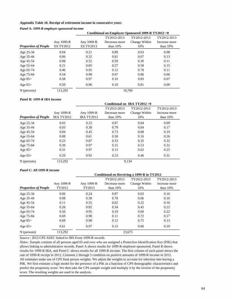
Appendix Table 10. Receipt of retirement income in consecutive years

Panel A: 1099-R employer-sponsored income

Proportion of PeopleAny 1099-R ES TY2012

Any 1009-RES TY2013

TY2012-2013 Decrease more

than 10%

TY2012-2013 Change Within

10%

TY2012-2013 Increase more

than 10%

Age 25-34 0.04 0.21 0.89 0.03 0.08Age 35-44 0.06 0.32 0.81 0.07 0.13Age 45-54 0.08 0.52 0.59 0.30 0.11Age 55-64 0.21 0.85 0.27 0.58 0.15Age 65-74 0.46 0.95 0.12 0.78 0.11Age 75-84 0.54 0.98 0.07 0.86 0.06Age 85+ 0.58 0.97 0.10 0.83 0.07

Age 65+ 0.50 0.96 0.10 0.81 0.09

N (persons) 113,292

Panel B: 1099-R IRA income

Proportion of PeopleAny 1099-R IRA TY2012

Any 1099-RIRA TY2013

TY2012-2013 Decrease more

than 10%

TY2012-2013 Change Within

10%

TY2012-2013 Increase more

than 10%

Age 25-34 0.02 0.23 0.87 0.04 0.09Age 35-44 0.03 0.38 0.79 0.04 0.17Age 45-54 0.04 0.45 0.73 0.08 0.19Age 55-64 0.08 0.61 0.58 0.16 0.26Age 65-74 0.23 0.87 0.33 0.35 0.32Age 75-84 0.39 0.97 0.15 0.53 0.32Age 85+ 0.31 0.97 0.13 0.62 0.25

Age 65+ 0.29 0.92 0.23 0.46 0.31

N (persons) 113,292

Panel C: All 1099-R income

Proportion of PeopleAny 1099-R

TY2012Any 1099-R

TY2013

TY2012-2013 Decrease more

than 10%

TY2012-2013 Change Within

10%

TY2012-2013 Increase more

than 10%

Age 25-34 0.06 0.24 0.87 0.03 0.10Age 35-44 0.08 0.38 0.78 0.06 0.16Age 45-54 0.11 0.55 0.62 0.22 0.16Age 55-64 0.26 0.82 0.34 0.45 0.22Age 65-74 0.56 0.95 0.19 0.60 0.22Age 75-84 0.69 0.98 0.11 0.72 0.17Age 85+ 0.69 0.98 0.12 0.75 0.13

Age 65+ 0.61 0.97 0.15 0.66 0.19

N (persons) 113,292

Source : 2013 CPS ASEC linked to IRS Form 1099-R records.Notes : Sample consists of all persons aged 65 and over who are assigned a Protection Identification Key (PIK) that allows linking to administrative records. Panel A shows results for 1099-R employer-sponsored, Panel B shows results for 1099-R IRA, and Panel C shows results for all 1099-R income. The first column of each panel shows the rate of 1099-R receipt in 2012. Columns 2 through 5 condition on positive amounts of 1099-R income in 2012. All estimates make use of CPS final person weights. We adjust the weights to account for selection into having a PIK. We first estimate a logit model for the presence of a PIK as a function of CPS demographic characteristics and predict the propensity score. We then take the CPS sample weight and multiply it by the inverse of the propensity score. The resulting weights are used in the analysis.

Conditional on Employer-Sponsored 1099-R TY2012 >0

Conditional on IRA TY2012 >0

Conditional on Receiving a 1099-R in TY2012

23,675

9,134

18,760

84

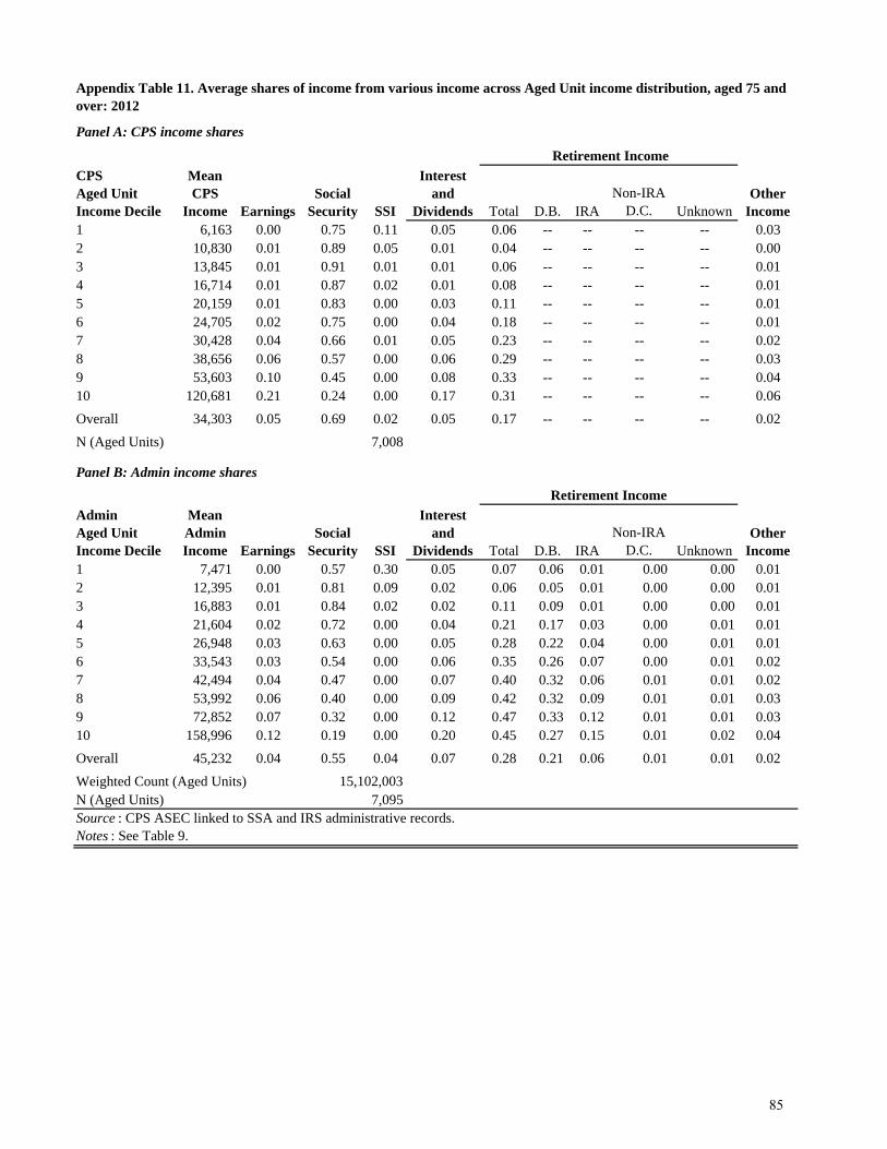
Total D.B. IRANon-IRA

D.C. Unknown1 6,163 0.00 0.75 0.11 0.05 0.06 -- -- -- -- 0.032 10,830 0.01 0.89 0.05 0.01 0.04 -- -- -- -- 0.003 13,845 0.01 0.91 0.01 0.01 0.06 -- -- -- -- 0.014 16,714 0.01 0.87 0.02 0.01 0.08 -- -- -- -- 0.015 20,159 0.01 0.83 0.00 0.03 0.11 -- -- -- -- 0.016 24,705 0.02 0.75 0.00 0.04 0.18 -- -- -- -- 0.017 30,428 0.04 0.66 0.01 0.05 0.23 -- -- -- -- 0.028 38,656 0.06 0.57 0.00 0.06 0.29 -- -- -- -- 0.039 53,603 0.10 0.45 0.00 0.08 0.33 -- -- -- -- 0.0410 120,681 0.21 0.24 0.00 0.17 0.31 -- -- -- -- 0.06Overall 34,303 0.05 0.69 0.02 0.05 0.17 -- -- -- -- 0.02N (Aged Units)

Total D.B. IRANon-IRA

D.C. Unknown1 7,471 0.00 0.57 0.30 0.05 0.07 0.06 0.01 0.00 0.00 0.012 12,395 0.01 0.81 0.09 0.02 0.06 0.05 0.01 0.00 0.00 0.013 16,883 0.01 0.84 0.02 0.02 0.11 0.09 0.01 0.00 0.00 0.014 21,604 0.02 0.72 0.00 0.04 0.21 0.17 0.03 0.00 0.01 0.015 26,948 0.03 0.63 0.00 0.05 0.28 0.22 0.04 0.00 0.01 0.016 33,543 0.03 0.54 0.00 0.06 0.35 0.26 0.07 0.00 0.01 0.027 42,494 0.04 0.47 0.00 0.07 0.40 0.32 0.06 0.01 0.01 0.028 53,992 0.06 0.40 0.00 0.09 0.42 0.32 0.09 0.01 0.01 0.039 72,852 0.07 0.32 0.00 0.12 0.47 0.33 0.12 0.01 0.01 0.0310 158,996 0.12 0.19 0.00 0.20 0.45 0.27 0.15 0.01 0.02 0.04Overall 45,232 0.04 0.55 0.04 0.07 0.28 0.21 0.06 0.01 0.01 0.02Weighted Count (Aged Units)N (Aged Units)

Other Income

Interest and

Dividends

EarningsSocial

Security SSI

Interest and

DividendsOther

Income

7,095

7,008

Appendix Table 11. Average shares of income from various income across Aged Unit income distribution, aged 75 and over: 2012

Source : CPS ASEC linked to SSA and IRS administrative records.Notes : See Table 9.

SSISocial

SecurityEarnings

Mean Admin Income

15,102,003

Panel A: CPS income shares

Retirement Income

Panel B: Admin income shares

Retirement Income

Admin Aged Unit Income Decile

CPS Aged Unit Income Decile

Mean CPS

Income

85