Experimental Design & Analysis

Contrasts, Trend Analysis and Effects Sizes

February 6, 2007

Outline

Contrasts Trend analysis Effects sizes

Contrasts

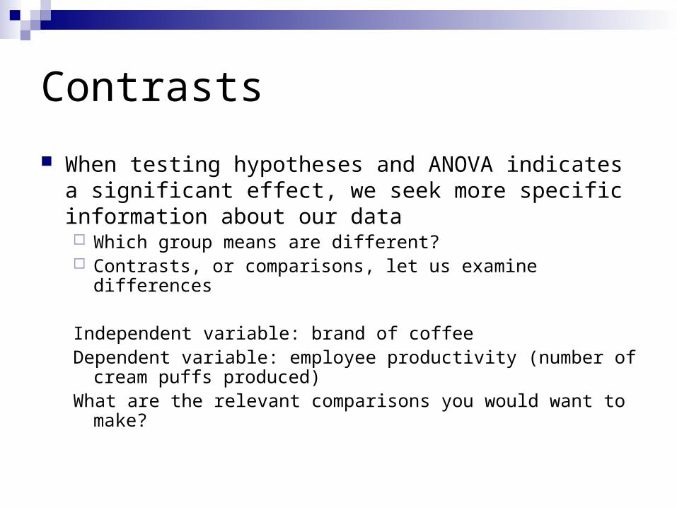
When testing hypotheses and ANOVA indicates a significant effect, we seek more specific information about our data Which group means are different? Contrasts, or comparisons, let us examine differences

Independent variable: brand of coffee Dependent variable: employee productivity (number of cream puffs

produced)What are the relevant comparisons you would want to make?

Contrasts

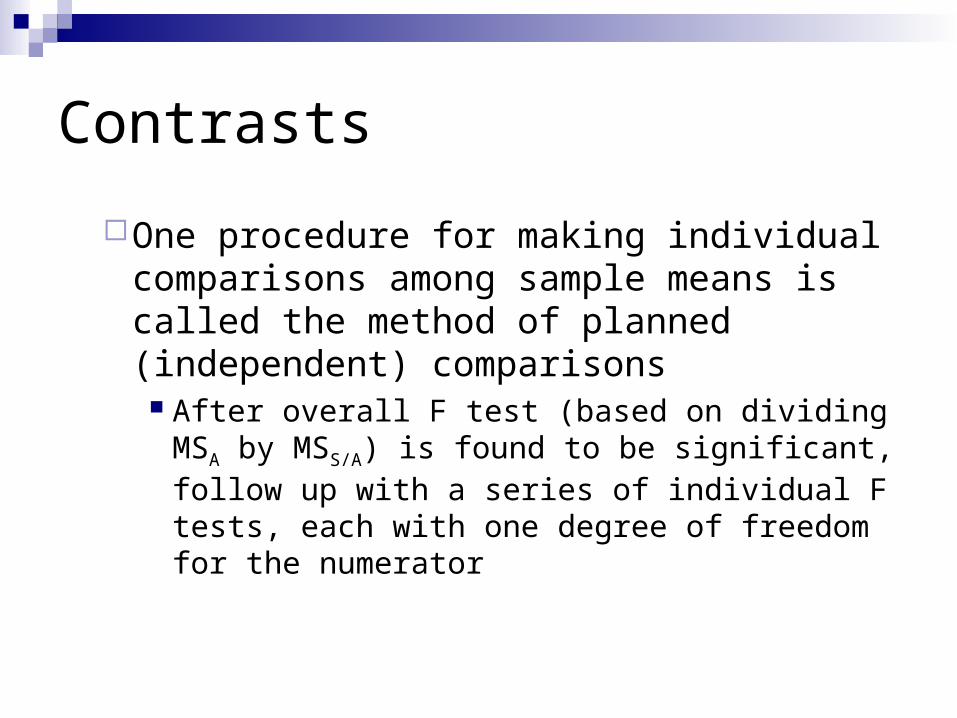
One procedure for making individual comparisons among sample means is called the method of planned (independent) comparisons

After overall F test (based on dividing MSA by MSS/A) is found to be significant, follow up with a series of individual F tests, each with one degree of freedom for the numerator

Contrasts

Planned comparisons (also called pairwise comparisons or single-df tests) give more information about what is happening in the data

Complex comparisons allow testing average of 2 or more groups with another group

Unplanned contrasts limited to (k-1) tests of significance

Contrasts

Suppose we are interested in the effects of coffee on employees’ cream-puff production

Starbucks, Peet’s, Maxwell House, Folgers, Sanka There are a possible total of a(a – 1)/2 comparisons In our coffee example: (5*4)/2 = 10 possible pairwise

comparisons Starbucks vs. each of the 4 other brands, Peet’s vs. each

of the other 3 brands, Maxwell House vs. 2 other brands, Folgers vs. Sanka

But not all of these makes sense

Coffee Contrasts

H01: X1 – X2 = 0

H02: X1 – X3 = 0

H03: X1 – X4 = 0

H04: X1 – X5 = 0

H05: X2 – X3 = 0

H06: X2 – X4 = 0

H07: X2 – X5 = 0

H08: X3 – X4 = 0

H09: X3 – X5 = 0

H010: X4 – X5 = 0

Coefficients for pairwise contrasts {1, -1}

Ψj = C1X1 + C2X2 + C3X3 + …+ CkXk where Σ Cj = 0 j=1

k

Coffee Contrasts

A comparison of the Sanka (decaf) with the other brands

Comparisons among the café brands and the store brands

Comparisons between the café brands (Starbucks and Peet’s)

Comparisons between the store brands (Maxwell House and Folgers)

(+1)X1 + (+1)X2 + (+1)X3 + (+1)X4 + (-4)X5

(+1)X1 + (-1)X2 + (0)X3 + (0)X4 + (0)X5

(+1)X1 + (+1)X2 + (-1)X3 + (-1)X4 + (0)X5

(0)X1 + (0)X2 + (+1)X3 + (-1)X4 + (0)X5

Contrasts

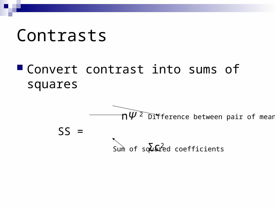
Convert contrast into sums of squares

nΨ 2

SS =

Σc2

Sum of squared coefficients

Difference between pair of means

Contrasts

Evaluate means by creating F ratio

F =MSΨ

MSS/A

Contrasts

Contrasts that flow from the omnibus F test and are followed up with pairwise comparisons allow “continuity”

When overall F test is not significant, t tests of theoretically important mean comparisons may be appropriate

Experimentwise Error Rate

Type I error rate accumulates over a family of tests

If each test is evaluated at α significance level, probability of avoiding Type I error is 1- α

Probability of making no familywise errors with c tests = (1- α)c

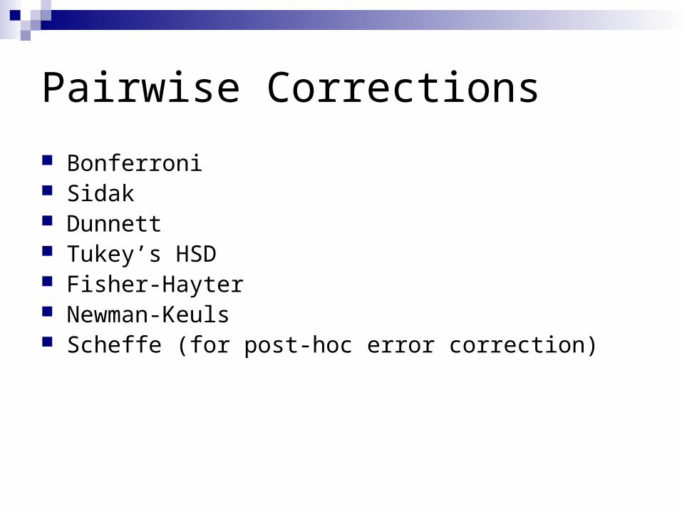
Pairwise Corrections

Bonferroni Sidak Dunnett Tukey’s HSD Fisher-Hayter Newman-Keuls Scheffe (for post-hoc error correction)

Trend Analysis

If an experiment contains a quantitative IV then the shape of the function relating the levels of this quantitative IV to the DV is often of interest Trend analysis can be

used to test different aspects of the shape of the function relating the IV (advertising repetitions) and the DV (sales)

0

200

400

600

800

1000

2 4 6 8

Sales

Repetitions

Trend Analysis

The linear component of trend is used to test whether there is an overall increase (or decrease) in the DV as the IV increases A test of the linear

component of trend is a test of whether this increase in sales is significant

0

200

400

600

800

1000

2 4 6 8

Sales

Repetitions

Trend Analysis

If there were a perfectly linear relationship between repetitions and sales, then no components of trend other than the linear would be present

The quadratic component of trend is used to test whether the slope increases (or decreases) as the independent variable increases 0

200

400

600

800

1000

2 4 6 8

Sales

Repetitions

Trend Analysis

Trend analysis is computed as a set of orthogonal comparisons using a particular set of coefficients

Each set of comparisons is tested for significance Linear Quadratic Cubic

Trend Analysis

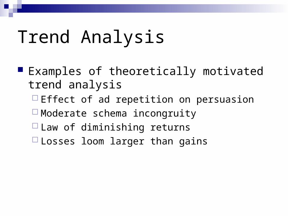
Examples of theoretically motivated trend analysis Effect of ad repetition on persuasion Moderate schema incongruity Law of diminishing returns Losses loom larger than gains

Effect Sizes

Effect size is a name given to a family of indices that measure the magnitude of a treatment effect Unlike significance tests, effect size indices are independent of sample size Measures are the common currency of meta-analyses

Two ways to think about effect sizes The standardized difference between means

d = (m1 – m2)/s Appropriate when comparing two groups

How much of variability can be attributed to treatments Effect size is ratio of variability explained to total variability or the SSEffect/SSTotal

Expressed as R2

Appropriate for > 2 groups

Check out effect-size calculators at http://davidmlane.com/hyperstat/effect_size.html

Effect Sizes

Effect sizes expressed as d and R2 are descriptive statistics

In the populationω2 = (σTotal

2 - σError2)/ σTotal

2

ω2 = SSA – (a-1) MSS/A

SStotal + MSS/A

ω2 = (a - 1) (F -1)

(a - 1) (F -1) + (an)

Effect Sizes

Properties of ω2: Varies between 0 and 1 (except in a fluke occurrence

when F < 1, (negative ω2) then treat it like zero) Unlikely to get very high estimates of ω2 because

behavioral research has so much error variance Cohen’s guidelines

.01 = small .5 = moderate .8 = large

Effect Sizes

0.2 effect size corresponds to the difference between the heights of 15 and 16 year old girls in the US

0.5 effect size corresponds to the difference between the heights of 14 and 18 year old girls

0.8 effect size equates to the difference between the heights of 13 and 18 year old girls