does access to secondary education affectftp.iza.org/dp6507.pdfdoes access to secondary education...

DI

SC

US

SI

ON

P

AP

ER

S

ER

IE

S

Forschungsinstitut zur Zukunft der ArbeitInstitute for the Study of Labor

Does Access to Secondary Education AffectPrimary Schooling? Evidence from India

IZA DP No. 6507

April 2012

Abhiroop MukhopadhyaySoham Sahoo

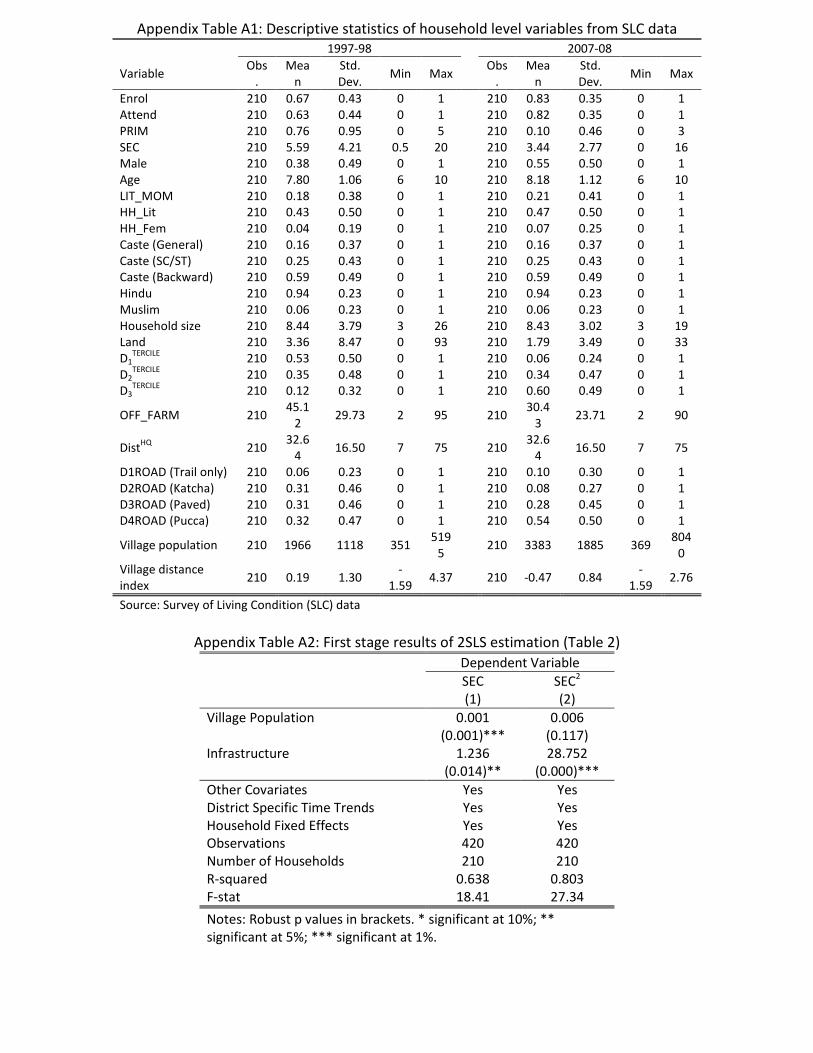
Does Access to Secondary Education

Affect Primary Schooling? Evidence from India

Abhiroop Mukhopadhyay Indian Statistical Institute, Delhi

and IZA

Soham Sahoo Indian Statistical Institute, Delhi

Discussion Paper No. 6507 April 2012

IZA

P.O. Box 7240 53072 Bonn

Germany

Phone: +49-228-3894-0 Fax: +49-228-3894-180

E-mail: [email protected]

Any opinions expressed here are those of the author(s) and not those of IZA. Research published in this series may include views on policy, but the institute itself takes no institutional policy positions. The Institute for the Study of Labor (IZA) in Bonn is a local and virtual international research center and a place of communication between science, politics and business. IZA is an independent nonprofit organization supported by Deutsche Post Foundation. The center is associated with the University of Bonn and offers a stimulating research environment through its international network, workshops and conferences, data service, project support, research visits and doctoral program. IZA engages in (i) original and internationally competitive research in all fields of labor economics, (ii) development of policy concepts, and (iii) dissemination of research results and concepts to the interested public. IZA Discussion Papers often represent preliminary work and are circulated to encourage discussion. Citation of such a paper should account for its provisional character. A revised version may be available directly from the author.

mailto:[email protected]

IZA Discussion Paper No. 6507 April 2012

ABSTRACT

Does Access to Secondary Education Affect Primary Schooling? Evidence from India*

This paper investigates if better access to secondary education increases enrolment in primary schools among children in the 6-10 age group. Using a household-level longitudinal survey covering 43 villages in a poor state in India, we find support for the hypothesis that better access to secondary education increases enrolment and attendance among children in the primary school-going age group. A 1 km decrease in the distance to the nearest secondary school increases the proportion of children in a household who are enroled in primary school by 6.5 percentage points. These results do not change significantly even after we account for endogenous placement of secondary schools and measurement error issues. Moreover, we find that the effect is consistent with what theory predicts: the marginal effect is larger for poorer households and boys (who are more likely to enter the labour force). Further, using a nationally representative survey for India (National Sample Survey 2007-08), we also provide some suggestive evidence that this effect may be quite widespread. This result gives support to the assertion that if the costs of post primary schooling are too high, as they would be if secondary schools are far away, parents have lesser interest in their children's education even at the primary stage. JEL Classification: I2, I20, I21 Keywords: primary schooling, returns to schooling, post primary schooling Corresponding author: Abhiroop Mukhopadhyay B 10 Indian Statistical Institute 7 S.J.S. Sansanwal Marg New Delhi 110016 India E-mail: [email protected]

* The authors wish to thank seminar participants at the Institute of Economic Growth, Delhi; participants of the Growth and Development Conference, Delhi; and The Indian Econometric Society Conference, Pondicherry for their comments. This research was funded by a research grant from the Planning and Policy Research Unit, Indian Statistical Institute, Delhi. Abhiroop Mukhopadhyay conducted research on this paper when he was Sir Ratan Tata Senior Fellow at the Institute of Economic Growth, Delhi (2010-11).

mailto:[email protected]

2

1. Introduction

The second Millennium Development Goal (MDG) of the United Nations aims at universalization of primary education by 2015. Despite best attempts and significant rises in enrolment in most developing countries, recent findings suggest that the target is unlikely to be met1. While access to primary schooling has improved substantially, high dropout rates are still a critical problem2

Studies specific to India have also shown similar results (Kingdon, 1998; Duraisamy, 2002; and Kingdon and Unni, 2001). On the other handsome other studies show that while the actual rate of return to primary schooling is high, parents believe that the first few years of schooling have lower returns than in the later years (Banerjee and Duflo, 2005 and 2011). These observations suggest that households may perceive education investment as lumpy;

. In India, major public policy initiatives like Sarva Shiksha Abhiyan (Education for All), the provision of a mid-day meal, free textbooks, uniforms, etc. aim to universalize elementary education and reduce disparity across regions, gender and social groups. In this context, two suggestions have been popular: to reduce the access barrier through the provision of community-based primary schools; and to improve the quality of schools in terms of physical infrastructure, teacher quality, etc. This paper raises a third issue: Does the possibility of continuation into higher levels of schooling affect primary schooling outcomes? In particular, we seek to investigate the effect of access to secondary education on primary school participation.

The decision of investment in the human capital of children is crucially linked to the perceived economic returns to education (Manski, 1996; Nguyen, 2008; and Jensen, 2010). The received wisdom from studies conducted in the past two decades is that the returns to education are concave, i.e., the marginal effect of an increment in the number of years of primary schooling is larger than the effect at higher levels (Psacharopoulos, 1994; Psacharopoulos and Patrinos, 2004). However, several recent studies show that the private returns to each extra year of education, in fact, rise with the level of education. A paper by Colclough et al (2010) refers to several studies on different countries that find this changing pattern of returns to education. Schultz (2004) finds that private returns in six African countries are highest at the secondary and post-secondary levels. Kingdon et al (2008) find a convex shape of the education–income relationship in 11 countries.

1 A fact sheet published by the United Nations in 2010 reveals that although enrolment in primary education in developing regions has increased from 83 percent in 2000 to 89 percent in 2008, yet this pace of progress is insufficient to meet the target by 2015. About 69 million school age children were out of school in 2008. 2 Statistics published by the United Nations show that the proportion of pupils in India starting grade 1 who reach last grade of primary education was only 68.5 percent in 2006 (http://unstats.un.org/unsd/mdg/SeriesDetail.aspx?srid=591). The report on elementary education in India published by the District Information System for Education (DISE) shows that the average dropout rate in primary level (grade 1 to 5) between 2006–07 and 2007–08 was 9.4 percent.

3

that significant economic returns require continuation to at least high school – households may find it worthwhile to educate their children only if they can reach that level. In light of this, better access to a post-primary school represents reduction in the cost of post-primary schooling and increases the possibility of continuation into higher levels of schooling. In doing so, it can become an important determinant of primary school participation.

This paper aims to empirically test the hypothesis that access to secondary schools affects primary schooling outcomes. Although the importance of access to schooling in determining educational outcomes has been well recognized in the literature (Duflo, 2001 and 2004; Glick and Sahn, 2006), most of it is on access to primary schooling and its effect on children. Therefore, a major supply side intervention for policymakers has been to increase the availability of primary schools to the community to encourage more school participation by the children. One commonly used measure of access is distance to school. Different studies have found that a reduction in distance to school improves enrolment, reduces dropout and improves test scores (Lavy, 1996; Bommier and Lambart, 2000; Brown and Park, 2002; Handa, 2002; and Burde and Linden, 2010).

Most of the literature addressing access examines the linkage between schooling outcomes at a particular level with the access to that level of schooling. Therefore, they have a static view of concentrating solely on the current cost of schooling. However, difficult access to post-primary schooling that reflects the future cost of schooling hinders the possibility of continuation to a higher level of education and can hence adversely affect schooling decisions even at the primary level. Only a few studies acknowledge the importance of access to post-primary schooling in determining outcomes at the primary level.

Lavy (1996) uses a cross-sectional data-set for rural Ghana and shows that distance to post-primary schools negatively affects primary school enrolment. He suggests that the effective fees for post-primary schooling should be reduced to induce more participation at the primary level. Results similar to Lavy (1996) have been found in studies by Burke and Beegle (2004) on Tanzania, by Vuri (2008) on Ghana and Guatemala and by Lincove (2009) on Nigeria. Hazarika (2001) uses a cross-sectional data-set on rural Pakistan and finds no impact of access to post-primary school on primary school enrolment of girls. His study indicates that if gains from post-primary schooling are low, as in the case for girls in Pakistan, access to it has no effect on primary school outcomes. Almost all of these studies base their analysis on cross-sectional data; hence, they are unable to control for time-invariant unobserved heterogeneity at the household level. Besides, while they have many villages, each village has few households; so they cannot control for village-level fixed effects. Moreover, apart from Lavy (1996), there is no discussion on endogenous placement of schools, which can be a potential source of bias in the estimates.

This paper uses a household-level longitudinal survey of 43 villages in Uttar Pradesh, a state in India, to test the hypothesis that better access to secondary education increases enrolment and attendance among children in the primary school-going age group. Using a

4

fixed effects regression, the paper finds that such an effect indeed exists. The results do not change even after we account for endogenous placement of secondary schools and measurement error issues. Moreover, we find that the effect is heterogeneous: the marginal effect is larger for smaller villages and for villages closer to bus stops. The effect is also larger for poorer households and boys (who are more likely to enter the labour force). Stratifying the sample by age cohorts, the paper finds larger effects on the enrolment of younger children and on the attendance of older children. Using a nationally representative survey for India (National Sample Survey 2007–08), we also provide some suggestive evidence that this effect may be quite widespread.

This study contributes to the existing literature by extensively examining how developments at higher levels of education influence decisions at much lower levels. This is especially relevant in a developing country where access to higher education is not universal. This paper indicates a robust causal relationship between access to secondary level and participation at the primary level3

To test our hypothesis, we provide evidence using data from a longitudinal follow-up of households first surveyed as a part of the World Bank's Living Standards Measurement Study (LSMS) in Uttar Pradesh, a state in India (this survey is also called the Survey of Living Conditions, or SLC). This is a two-period panel data on rural households in 43 villages from nine districts in eastern and southern Uttar Pradesh

. The analysis presented in this paper suggests that the goal of universal primary education cannot be achieved unless higher levels of schooling are made more accessible.

The paper is organized as follows. Section 2 describes the data used for our analysis. Section 3 explains the empirical methodology. Section 4 reports the results obtained from the main regressions. In Section 5, we show that our results are robust. Section 6 investigates if there are other pathways that explain our results. In Section 7, results are provided that show that the impact of secondary school access is heterogeneous. And the final section discusses the conclusions of the paper.

2. Data

4. The baseline data collection was undertaken in 1997–98 by the LSMS. The second round of data was collected in 2007–08 by the authors and funded by the University of Oxford and the World Bank5

3 Our study relates very well to the recent policy environment in India, where the Ministry of Human Resource Development has developed a framework for universalization of access to and improvement of quality at the secondary stage. Following Sarva Shiksha Abhiyan, setting up of a national mission on Rashtriya Madhyamik Shiksha Abhiyan (RMSA), or universalization of secondary education, is in process. 4 Uttar Pradesh is usually considered one of the most backward regions in the country. 5 Both surveys were conducted during the same time of the year – December to April. The data collected in 1997 was verified to the extent possible during the second survey. Household attrition rate for the sample was 13.8 percent.

. The survey comprised a village questionnaire that contained information on, among other things,

5

access to the nearest primary and secondary schools and a household questionnaire that had detailed information on various aspects of standard of living, including the schooling status of each child in the household.

For the purpose of our study, we use information on households with children in the 6–10 age group. There were 441 and 356 such households in 1997–98 and 2007–08 respectively. Among these households, there were 210 households with children in the relevant age group both in 1997–98 and 2007–08. We use data on these households in our panel methods6

Our two variables of interest are the proportion of children aged 6–10 years in households who are enrolled in schools, defined as enrol, and the proportion of children in the same age group in households that attend school. The SLC has detailed information on attendance. It reports the number of days in the past seven days that the child attended school

.

7

According to estimates from the SLC dataset, while enrol was 69.63 percent in 1997–98, it had increased to 82.1 percent by 2007–08. Based on our definition, while the attendance share was 64.57 percent in 1997–98, it had risen to 79.95 percent by 2007–08

. We define attend as the proportion of children in the household who have attended school at least three days in the last week.

8

Pooling the data from both rounds, we find a significant and negative correlation of -0.17 between the proportion of enrolled children at the primary level and distance to the nearest secondary school. However, this correlation coefficient does not take into account any other confounding factors that may have changed over time. Therefore, in the next section, we

.

We use information on distance-to-schools that have been collected during the village survey. Distance to the nearest primary, middle and secondary schools is measured from the village centre and reported in kilometres. The average distance to the nearest primary school has been reduced from 0.7 km to 0.1 km and to the nearest middle school from 2.5 km to 1.4 km. However, because both primary and middle schools were already very close on average to the villages in 1997–98, the change is modest. The change in the distance to the nearest secondary school has been spectacular, though. Figure 1 gives the distribution of distance to secondary schools. The average distance has reduced from 6.4 to 3.8 km.

6 Our most restrictive analysis using the balanced panel of households uses information on 1356 children over the two years. 7 Consistent with the baseline survey, holidays and unusual attendances because of family events are factored in while asking this question. For this small sub-sample, attendance on the last normal week is asked. While such self-reported data are not perfect, we are constrained not to change questions for the sake of uniformity. 8 The corresponding enrolment rate for children in the 6–10 age group increased from 68.94 percent in 1997–98 to 82.46 percent in 2007–08. The rise in the enrolment rate has been higher for girls (from 62.4 percent to 83.52 percent) as compared to boys (from 75.8 percent to 81.56 percent). Attendance rates show a similar trend.

6

specify econometric models and carry out multivariate analysis to look into the hypothesized causation more carefully.

3. Empirical Model

This section discusses an empirical model to test whether access to secondary schools increases schooling enrolment and attendance at the primary level. For ease of presentation, we refer to only enrolment in the empirical model; however, in testing, we test both enrolment and attendance.

For each household i living in village j at time t, let the proportion of children in the age group 6–10 years who are enrolled in school be . In our description below, the subscripts

are implicit.

The co-variates for explaining enrolment can usually be categorized into four:

• individual child level factors: gender, age;

• household characteristics: wealth, household education, social group, religion;

• school characteristics: access to schools, quality of schooling; and

• geographical characteristics: village/district characteristics.

Since S is defined at the household level, we transform child-level variables into their appropriate household counterparts: average age of children within the 6–10 age band (Age) and proportion of male children in the same age band (Male). To allow for non-linear impacts of age on enrolment, we include the square of average age (Age²).

Among other household-level variables, we include land size to control for wealth (land). The education level of decision makers in the household, especially of the mother, has often been found in literature to have an important impact on the educational outcome of children. In the SLC, the identity of the mother is known. Hence, we control for the education of the mothers by including the proportion of literate mothers (LITMOM)9

9 Consistent with our analysis, we look at mother of children aged 6 to 10.

. We also include a dummy variable to capture whether the household head is literate (HHLit). Moreover, previous literature has also found that the education outcomes of children are better when the household decision maker is a woman. Hence, we also include a dummy variable that indicates if the household head is a woman (HHFem). To allow for differential impacts across different castes, we also include dummy variables that represent the social group the household belongs to (SC/T: Scheduled Caste/Tribe, OBC: Other Backward Caste; the omitted category is the other less disadvantaged castes). Similarly, we allow for

7

different enrolment rates across different religious communities by including religion dummies; in particular, we create a dummy variable for Muslims (Muslim).

This paper concentrates on access to secondary schooling, a level that yields perceptible market returns. Our study found primary schools close to most villages but not secondary schools. We focus on secondary schooling, less likely than middle schooling to be susceptible to endogeneity. Secondary schools need a larger market size to be profitable because of the need for more infrastructure and relatively better trained teachers; their placement depends on the characteristics of a larger group of people than just a village. Indeed, even after their proliferation, they are still, on an average, 3.4 kmsaway from the villages. Hence, in our specification, we allow for access to the nearest primary and secondary schools. These variables measuring the distance to the nearest school are measured as continuous variables. We include a squared term of distance to secondary schooling to allow for non-linearity of this effect10

Let us refer to the distance to nearest primary school as PRIM. Moreover, the vector of the linear and the squared distance to the nearest relevant secondary school is referred to as SEC. While the inclusion of PRIM is standard in primary schooling regressions, the inclusion of distance to secondary schools is less standard

.

11

Recent literature on schooling has stressed the importance of the quality of schools. The quality of primary schools has been found to be significant in papers that investigate schooling outcomes. More crucially for our analysis, if secondary schools are present closer to villages where the quality of primary schools is good, then our estimators for the impact of access to secondary school would be inconsistent. Thus, we include quality of the village primary school as a regressor. We include three terciles of quality

. We hypothesize that if access to the nearest secondary school is found to be statistically significant after controlling for primary school access, the hypothesis that the possibility of continuation plays a significant role in primary school enrolment will be credible. Indeed, if parents perceive that only returns to higher levels of schooling are worth the investment of sending children to school, then they would be unlikely to enrol their children in primary schools if secondary schools are far away.

constructed by

principle components over various features of infrastructure12

10 Given very small distances of primary schooling from the villages, we omit the square of distance to primary schooling from our specification. 11 It must be pointed out here that inclusion of the quadratic term in distance is less common. However, we include them because we posit that marginal changes in distances matter more when the distances are closer. 12 The features of school quality considered in the analysis are: type of structure, main flooring material, whether the school has classrooms, number of classrooms, whether the classes are held inside classrooms, whether the school has usable blackboards, whether desks are provided to the students, whether mid-day meal is provided, and the proportion of teachers present on the day of survey.

.

8

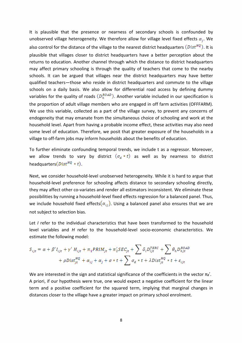
It is plausible that the presence or nearness of secondary schools is confounded by unobserved village heterogeneity. We therefore allow for village level fixed effects . We

also control for the distance of the village to the nearest district headquarters . It is

plausible that villages closer to district headquarters have a better perception about the returns to education. Another channel through which the distance to district headquarters may affect primary schooling is through the quality of teachers that come to the nearby schools. It can be argued that villages near the district headquarters may have better qualified teachers—those who reside in district headquarters and commute to the village schools on a daily basis. We also allow for differential road access by defining dummy variables for the quality of roads . Another variable included in our specification is

the proportion of adult village members who are engaged in off farm activities (OFFFARM). We use this variable, collected as a part of the village survey, to prevent any concerns of endogeneity that may emanate from the simultaneous choice of schooling and work at the household level. Apart from having a probable income effect, these activities may also need some level of education. Therefore, we posit that greater exposure of the households in a village to off-farm jobs may inform households about the benefits of education.

To further eliminate confounding temporal trends, we include t as a regressor. Moreover, we allow trends to vary by district as well as by nearness to district

headquarters .

Next, we consider household-level unobserved heterogeneity. While it is hard to argue that household-level preference for schooling affects distance to secondary schooling directly, they may affect other co-variates and render all estimators inconsistent. We eliminate these possibilities by running a household-level fixed effects regression for a balanced panel. Thus,

we include household fixed effects . Using a balanced panel also ensures that we are

not subject to selection bias.

Let I refer to the individual characteristics that have been transformed to the household level variables and H refer to the household-level socio-economic characteristics. We estimate the following model:

We are interested in the sign and statistical significance of the coefficients in the vector π₂′. A priori, if our hypothesis were true, one would expect a negative coefficient for the linear term and a positive coefficient for the squared term, implying that marginal changes in distances closer to the village have a greater impact on primary school enrolment.

9

The decision to run a household fixed effects model is not without a cost. Balancing cuts sample size and reduces efficiency. Given that secondary schools usually cater to bigger populations, the use of village dummies alone should lead to consistent estimation if we feel other co-variates are not correlated to . Lavy (1996) uses this identification strategy in his

cross-sectional analysis13

• a primary school of the highest quality (relatively speaking) in a village increases the share of enrolment by 0.248 but has no impact on attendance;

. However, household-level unobservables could still lead to inconsistent estimation for reasons pointed out above. For the sake of comparison, therefore, we also report results with just village fixed effects and a larger number of households (since we can now use all households with children aged 6–10 years in either round).

4. Main Results

While columns (1) and (2) in Table 1 report results with household fixed effects, columns (3) and (4) present a comparison using only village fixed effects. Results using column (1) and (2) show that while distance to primary school has no effect, distance to secondary schools does. The relationship is negative but the marginal impact of a drop in distance is less at large distances. This implies that the marginal effect of a 1 km-decrease in distance to secondary school on the share of children enrolled, evaluated at the mean distance in 2007–08 (3.34 km), is 0.065. The marginal effect on attendance is slightly lower at 0.060. The insignificance of distance to primary school for both variables for this sample is not surprising because most villages already had a primary school nearby even in 1997–98, as shown earlier.

Everything else turns out insignificant, barring the third tercile of primary school quality (in the case of enrolment), the share of proportion of adult members doing off-farm labour, road access variables and the time trend (for attendance). We find that

• a unit increase in the percentage of adult members in off farm employment raises both enrolment and attendance by 0.004; and

• a better road increases the probability of both enrolment and attendance, though this increase is highest for paved roads14

The insignificance of the rest of the variables could be driven by low temporal variation. Besides, creating the balanced panel required dropping households and led to inefficiency. Therefore, that our result on secondary schooling is obtained despite this inefficiency suggests that this effect is strong.

.

13 In addition, Lavy (1996) finds that secondary schools are very far from villages. Therefore, he does not instrument for the distance to the nearest secondary school. 14 While all weather roads (pucca) roads come out to be significant for attendance, their magnitude is less than that for paved. This is slightly puzzling but could be caused by slight misclassification between paved and "pucca".

10

How do our results compare when we include only village fixed effects and include all households that have children in either survey? The results that correspond to distance to the nearest secondary school still survive, though they are muted. The marginal effect is again negative and decreasing in distance. The marginal effect on enrolment of a kilometre-drop in distance to the nearest secondary school is 0.037 (evaluated at a mean distance of 3.44 km) whereas the marginal effect is 0.035 for attendance. This underestimates the effect of distance to secondary schools and suggests the need for controlling for household-specific fixed effects. Other significant results include the important role of a literate mother (marginal effect of 0.059 for enrolment and 0.071 for attendance), a literate household head (a marginal effect of 0.14 for both variables) and female head of the family (0.109 for enrol and 0.093 for attend). We also find that a greater proportion of children from households with more land are likely to both enrol in and attend primary school (a marginal effect of 0.007). As before, the share of off farm employment plays a positive role in both enrolment and attendance. Similarly, dummy variables for road access are positive and significant for both enrolment and attendance15

Even with individual and village fixed effects, one could contend that secondary schools come up endogenously. Since secondary schools need bigger markets, they may be more likely to come up in bigger villages. Indeed, our sample has villages that have grown over time. It could well be the case that some of the growing villages were able to attract secondary schools. However, we assume that controlling for this effect, such expansion should have no additional impact on the decision to send children to school. We therefore posit that village population (Village Population) can be used as an instrument for distance to secondary schools. In addition, following Lavy (1996), we also use changing distance to other institutions of development as another instrument

.

5. Robustness

In this section, we subject our specification to robustness checks. First, we want to know if any endogeneity in secondary school placements is driving our result. We address this by running a 2 SLS estimation procedure. Second, we consider the implication of running the regression at the household level instead of at the child level. Third, we test if our results are affected by measurement errors and outliers.

5.1 Instrumental Variables

16

15 A pure pooled OLS with no village level fixed effects yields many more significant variables. However, insofar as our results on access to secondary schooling survive all specifications, we do not forsake the fixed effects estimation models. 16 Lavy (1996) used distance to public telephone and post office as instruments for distance to middle school.

. We construct an index variable by principal component analysis: distance to the nearest telephone booth, police station,

11

public distribution shop and bank (Infrastructure)17

We have a linear and a square term of distance to secondary schools that are potentially endogenous. Given our two instruments, our model is just identified

. The implicit assumption is that improving access to village facilities is correlated with opening secondary schools but has no incremental impact on schooling decisions once we have controlled for other regressors.

18

The results in Table 2 show that in the case of both attendance and enrolment, we get the same qualitative result

.

19

Given these coefficients, our qualitative result that highlights the importance of access to secondary schools goes through. When the dependent variable is enrolment, the marginal effect of a change in distance to secondary school using fixed effects and instruments is similar to that obtained using just fixed effects. In case of attendance, the fixed effects model slightly underestimates the effect. Given this evidence, we report fixed effects regressions in the rest of the paper

. The linear term is negative and the square term is positive, thus replicating the same relationship. Moreover, they are both significant. Reassuringly, the magnitude of the effect is very similar for enrolment. The marginal effect at the mean for 2007–08 is now 0.061 (as compared to 0.065 in the household fixed effects model) and 0.086 for attendance (as compared to 0.060 in the household fixed effects model).

20

So far, the results obtained from household-level analysis have supported our hypothesis that access to secondary schooling does play a significant role in determining primary school participation. To further examine the robustness of these results, we conduct child-level analysis with household fixed effects. Hence, the unit of observation becomes specific to a child instead of a household. The dependent variable is binary enrolment or attendance. We

.

5.2 Unit of Analysis

17 It may be argued that access to telephone booth is not very relevant with the advent of mobile phones. Our results do not change when we drop this from the index. 18 Alternatively, we have also considered Village Population and its square as instruments. Results are similar and are available on request. 19 First stage results (Appendix Table A2) show that for both the linear term and the quadratic term, there is a positive coefficient for village population and distance to village infrastructure. We use changes over time to estimate these relationships; hence, while the latter coefficient is intuitive, the former coefficient points out that the distance to secondary schools has decreased more for villages showing smaller changes in population. However, in our sample, smaller villages show smaller changes in population. Hence, the distances have come down more for smaller villages. The F stats for the overall fit of the two first stage regressions are 18.41 and 27.34. 20 2 SLS estimation often causes increase in inefficiency. When we stratify our data further to look at heterogeneous effects, and keep the balanced panel structure, we are left with small number of observations for each cut. We abstain from causing further efficiency problems by conducting 2 SLS estimation. Suffice it to say, for most specifications, our results go through and in case, they are insignificant, they still retain the same qualitative relationship.

12

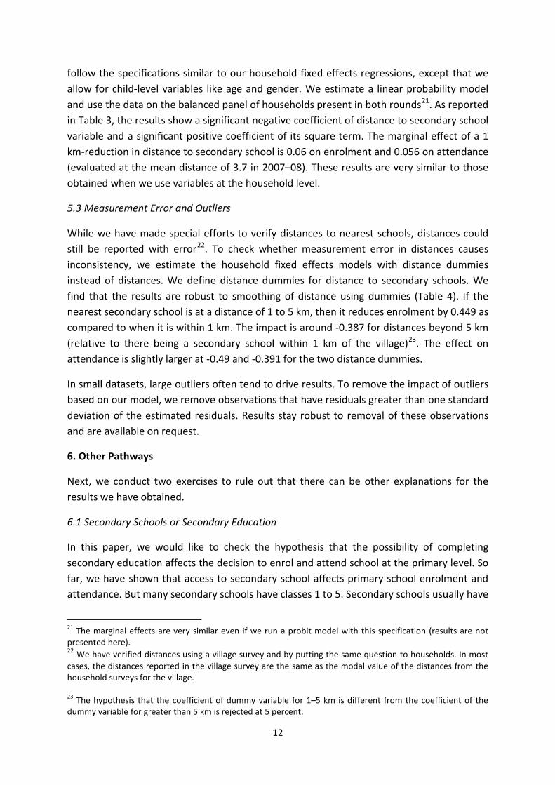
follow the specifications similar to our household fixed effects regressions, except that we allow for child-level variables like age and gender. We estimate a linear probability model and use the data on the balanced panel of households present in both rounds21

While we have made special efforts to verify distances to nearest schools, distances could still be reported with error

. As reported in Table 3, the results show a significant negative coefficient of distance to secondary school variable and a significant positive coefficient of its square term. The marginal effect of a 1 km-reduction in distance to secondary school is 0.06 on enrolment and 0.056 on attendance (evaluated at the mean distance of 3.7 in 2007–08). These results are very similar to those obtained when we use variables at the household level.

5.3 Measurement Error and Outliers

22. To check whether measurement error in distances causes inconsistency, we estimate the household fixed effects models with distance dummies instead of distances. We define distance dummies for distance to secondary schools. We find that the results are robust to smoothing of distance using dummies (Table 4). If the nearest secondary school is at a distance of 1 to 5 km, then it reduces enrolment by 0.449 as compared to when it is within 1 km. The impact is around -0.387 for distances beyond 5 km (relative to there being a secondary school within 1 km of the village)23

In this paper, we would like to check the hypothesis that the possibility of completing secondary education affects the decision to enrol and attend school at the primary level. So far, we have shown that access to secondary school affects primary school enrolment and attendance. But many secondary schools have classes 1 to 5. Secondary schools usually have

. The effect on attendance is slightly larger at -0.49 and -0.391 for the two distance dummies.

In small datasets, large outliers often tend to drive results. To remove the impact of outliers based on our model, we remove observations that have residuals greater than one standard deviation of the estimated residuals. Results stay robust to removal of these observations and are available on request.

6. Other Pathways

Next, we conduct two exercises to rule out that there can be other explanations for the results we have obtained.

6.1 Secondary Schools or Secondary Education

21 The marginal effects are very similar even if we run a probit model with this specification (results are not presented here). 22 We have verified distances using a village survey and by putting the same question to households. In most cases, the distances reported in the village survey are the same as the modal value of the distances from the household surveys for the village. 23 The hypothesis that the coefficient of dummy variable for 1–5 km is different from the coefficient of the dummy variable for greater than 5 km is rejected at 5 percent.

13

better quality, at least in terms of infrastructure, than standalone primary schools. It may be that children go for their primary education to a secondary school as it opens up nearer. In this case, our results would give further evidence, indirectly, to the importance of better quality.

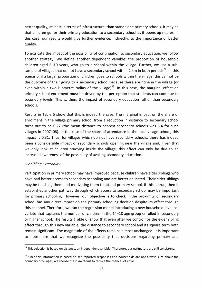
To extricate the impact of the possibility of continuation to secondary education, we follow another strategy. We define another dependent variable: the proportion of household children aged 6–10 years, who go to a school within the village. Further, we use a sub-sample of villages that do not have a secondary school within 2 km in both periods24. In this scenario, if a larger proportion of children goes to schools within the village, this cannot be the outcome of their going to a secondary school because there are none in the village (or even within a two-kilometre radius of the village)25

Participation in primary school may have improved because children have elder siblings who have had better access to secondary schooling and are better educated. Their elder siblings may be teaching them and motivating them to attend primary school. If this is true, then it establishes another pathway through which access to secondary school may be important for primary schooling. However, our objective is to check if the proximity of secondary school has any direct impact on the primary schooling decision despite its effect through this channel. Therefore, we run the regression model introducing a new household-level co-variate that captures the number of children in the 14–18 age group enrolled in secondary or higher school. The results (Table 6) show that even after we control for the elder sibling effect through this new variable, the distance to secondary school and its square term both remain significant. The magnitude of the effects remains almost unchanged. It is important to note here that we recognize the possibility that decisions regarding primary and

. In this case, the marginal effect on primary school enrolment must be driven by the perception that students can continue to secondary levels. This is, then, the impact of secondary education rather than secondary schools.

Results in Table 5 show that this is indeed the case. The marginal impact on the share of enrolment in the village primary school from a reduction in distance to secondary school turns out to be 0.27 (the mean distance to nearest secondary schools was 5.4 for such villages in 2007–08). In the case of the share of attendance in the local village school, this impact is 0.31. Thus, for villages which do not have secondary schools, there has indeed been a considerable impact of secondary schools opening near the village and, given that we only look at children studying inside the village, this effect can only be due to an increased awareness of the possibility of availing secondary education.

6.2 Sibling Externality

24 This selection is based on distance, an independent variable. Therefore, our estimators are still consistent. 25 Since this information is based on self-reported responses and households are not always sure about the boundary of villages, we choose the 2 km radius to reduce the chances of error.

14

secondary schooling of children are determined simultaneously in a household. However, our objective is not to estimate the causal effect of siblings; rather, we seek to show that our main results remain unperturbed even if we account for a possible correlation between the education of primary school age children and their older counterparts.

7. Heterogeneity of Effect

In this section, we investigate the heterogeneity of impact of access to secondary schools. To begin with, we look at the differential impact on villages of differing baseline sizes. Smaller villages, more distant from schools in the base year, may experience different changes relative to larger villages. We also look at how the impact of access to secondary schools depends on the village access to a bus stop. Thereafter, we investigate if the impact of the access to secondary schools varies by household characteristics. We look at whether households that have less than median landholdings have impacts different from those that are in the top half of the land distribution (in the base year). In the end, we investigate if the impacts are heterogeneous across different age groups and vary by gender.

To begin with, let us investigate if the impact of better access to secondary schools varies by the size of the village. We define small villages as ones where the number of households are less than 200 in the base year and large villages where the households are more than 20026

Does the impact of access to secondary schools vary with transport infrastructure? To investigate this, Table 8 reports the results using a formulation where we interact a dummy variable that measures if there is a bus stop within 1.5 km radius of the village (BUS) with the distance to the nearest bus stop

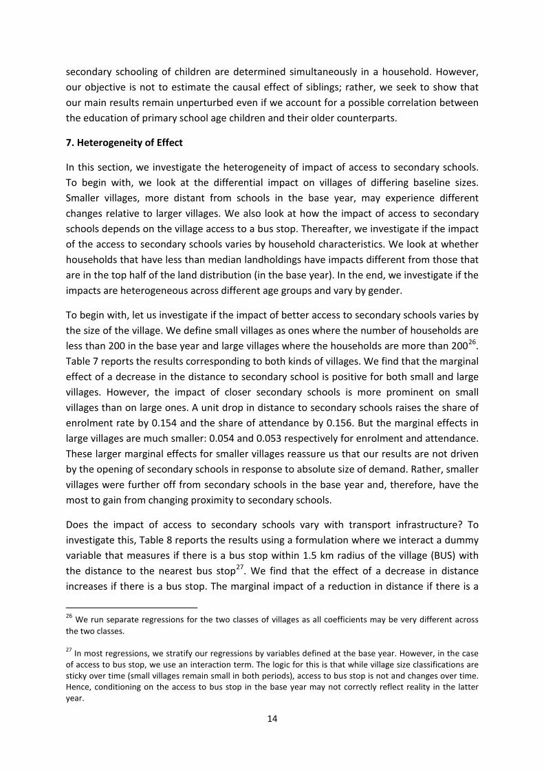
. Table 7 reports the results corresponding to both kinds of villages. We find that the marginal effect of a decrease in the distance to secondary school is positive for both small and large villages. However, the impact of closer secondary schools is more prominent on small villages than on large ones. A unit drop in distance to secondary schools raises the share of enrolment rate by 0.154 and the share of attendance by 0.156. But the marginal effects in large villages are much smaller: 0.054 and 0.053 respectively for enrolment and attendance. These larger marginal effects for smaller villages reassure us that our results are not driven by the opening of secondary schools in response to absolute size of demand. Rather, smaller villages were further off from secondary schools in the base year and, therefore, have the most to gain from changing proximity to secondary schools.

27

26 We run separate regressions for the two classes of villages as all coefficients may be very different across the two classes. 27 In most regressions, we stratify our regressions by variables defined at the base year. However, in the case of access to bus stop, we use an interaction term. The logic for this is that while village size classifications are sticky over time (small villages remain small in both periods), access to bus stop is not and changes over time. Hence, conditioning on the access to bus stop in the base year may not correctly reflect reality in the latter year.

. We find that the effect of a decrease in distance increases if there is a bus stop. The marginal impact of a reduction in distance if there is a

15

bus stop is 0.09 on enrolment (0.07 for attendance) and 0.06 (0.062 for attendance) when there is no bus stop. This result makes since the distance to the nearest secondary school measures the perception of how difficult it is to get to the next level of schooling.. In so far as most children would need a bus to go to these schools, our results point out that the impact of continuation kicks in when there is a complementary bus service. It therefore points out the need for developing infrastructure to reap these benefits.

. Economic theory suggests that the effect of access to secondary schools should vary with wealth. It is likely that a change in access cost will have a largereffect on poor households.. To check if this is indeed true, we carry out the regression separately for households whose landholding in 1997 was below the median level and for the ones above it. The results suggest that while we get significant effects for both groups, the magnitude is higher for households below the median level of landholding. The marginal effect of a 1 km decrease in distance—on enrolment—for poorer households (evaluated at 3 km, the mean of the sample in 2007–08) is 0.076 (for attendance: 0.063). The corresponding marginal effect for richer households (evaluated at the sample mean of 3.9 km) is lesser at 0.041 (0.053 for attendance). This result is intuitive as the cost of continued schooling binds most for poorer households. Hence, the impact of reduction of schooling must be higher for them28

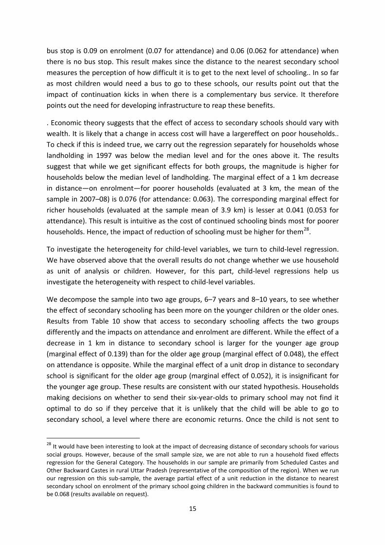
We decompose the sample into two age groups, 6–7 years and 8–10 years, to see whether the effect of secondary schooling has been more on the younger children or the older ones. Results from Table 10 show that access to secondary schooling affects the two groups differently and the impacts on attendance and enrolment are different. While the effect of a decrease in 1 km in distance to secondary school is larger for the younger age group (marginal effect of 0.139) than for the older age group (marginal effect of 0.048), the effect on attendance is opposite. While the marginal effect of a unit drop in distance to secondary school is significant for the older age group (marginal effect of 0.052), it is insignificant for the younger age group. These results are consistent with our stated hypothesis. Households making decisions on whether to send their six-year-olds to primary school may not find it optimal to do so if they perceive that it is unlikely that the child will be able to go to secondary school, a level where there are economic returns. Once the child is not sent to

.

To investigate the heterogeneity for child-level variables, we turn to child-level regression. We have observed above that the overall results do not change whether we use household as unit of analysis or children. However, for this part, child-level regressions help us investigate the heterogeneity with respect to child-level variables.

28 It would have been interesting to look at the impact of decreasing distance of secondary schools for various social groups. However, because of the small sample size, we are not able to run a household fixed effects regression for the General Category. The households in our sample are primarily from Scheduled Castes and Other Backward Castes in rural Uttar Pradesh (representative of the composition of the region). When we run our regression on this sub-sample, the average partial effect of a unit reduction in the distance to nearest secondary school on enrolment of the primary school going children in the backward communities is found to be 0.068 (results available on request).

16

school in his initial years, it is less likely that he/she will be enrolled in a primary school at a later age (8–10 years) in response to a change in access to secondary school. Hence, the effect on enrolment is larger for the younger age group. The results on attendance suggest that the older age groups start to lose interest and attend school less if there is no possibility of future continuation. This may explain their subsequent dropping out and why many children stop going to school when they get older despite higher enrolment rates for younger age groups.

Next, we examine if the effects vary by gender. Results in Table 11 show that while distance to secondary schools affects enrolment for boys (the results for attendance are also very close with p values of 0.11 and 0.135 for the linear and square term), there are no effects for girls (though the effect on the linear term for enrolment is close to significance with a p value of 0.138). This differential impact has two explanations.

First, recall that we hypothesize that the effect of secondary schooling comes from the possibility to earn economic returns after schooling. However, in rural areas, it is less likely for educated women to seek jobs29

It may be contended that our results are specific to the small part of India that our sample represents. Therefore, in this section, we provide additional evidence that suggests that our (qualitative) results are general. We do so by analyzing the same effect using a cross-sectional sample for rural India collected by the National Sample Survey. The National Sample Survey Organisation (NSSO) conducts nationally representative household surveys on "participation and expenditure in education" once in 10 years. We use the most recent education survey (64th Round) by NSSO conducted in 2007–08

. Therefore, the effect of continuation seems to be restricted to boys. Second, it is possible that distances to secondary schools are still far, although they have gone down. It is well known that parents do not send girls too far from the village. Therefore, it may be the case that the distances are such that this effect has not kicked in for girls.

8. Extending Hypothesis to a Nationally Representative Survey

30

29 This was also pointed out by Hazarika (2001). 30 Unlike in 64th round, the earlier NSSO education surveys did not have information on distance variables for post-primary schools. Therefore, only a static cross-sectional analysis is possible using the NSS data.

. Detailed information about the schooling status of each child in a household is reported in the dataset. The dataset also contains standard socioeconomic characteristics of the household. Crucial to the paper, it contains information on key variables of interest: distance to the nearest primary, upper-primary and secondary school for each household. This information allows us to examine the relationship between distance to the nearest secondary school and primary school participation.

17

Consistent with the analysis above, we restrict our analysis to children aged 6–10 years. The average share of children enrolled in a household is 89.7 percent while the average attendance share is 89.5 percent31. The access to secondary schooling is heterogeneous across rural India32

Analogous to the analysis above, we regress the proportion of children enrolled (attending) on individual characteristics (averaged at the household level): Age, Age², share of male children: MALE; household characteristics: A dummy variable representing whether the household head is literate: HHLIT, a dummy variable representing whether the household head is female: HHFEM, household size, dummy variables representing land categories, dummy variable representing whether the household is a Muslim: MUSLIM, dummy variables representing social groups: distance dummy variables for primary school (PRIM) and secondary schools (SEC)

. While 30.79 percent of the households have a secondary school within 1 km, for 17.08 percent of the households the nearest secondary school is located at a distance of more than 5 km.

33

We provide two sets of results in Table 12. The first column corresponds to the proportion of children in the 6–10 age group enrolled in school and the second column to the proportion of children in the 6–10 age group who attend school. We do not focus as much on other variables but their results are as expected

. We control for sub-regional differences by using dummy variables. While the attempt has been to keep the same set of variables as the analysis above, we are constrained by the variables available in the dataset. For example, we cannot control for the quality of the village primary school or any other access variable.

It is important to begin by the remark that the results should be treated as only suggestive. Given the cross-sectional nature of data, we do not make any claims on causality. Indeed, the earlier part of our paper shows the importance of the panel structure. The results here are provided to indicate that the results from the previous section are not specific to our sample but are consistent with correlations observed in a nationally representative sample.

34

31 The estimated enrolment rate for these children at the all India level (rural) is 89 percent; (boys: 90.36 percent, girls: 87.42 percent). Attendance rates do not differ much from the enrolment figures: overall it is 88.76 percent (boys: 90.18 percent, girls: 87.12 percent). 32 NSS data validate our claim that a majority of the population have easy access to primary schools. The nearest primary school is at a distance less than 1 km for 91.88 percent of the households. 33The distance categories are specified in the National Sample Survey.

. Moving to the variables of interest,

34 We find that age (Age) has the usual increasing and concave relationship with enrolment. Since some children start school late, more children are found enrolled in school as one raises the age at initial induction ages. However, after a certain age, they are more likely to drop out. The proportion of males among children (Male) is positive and significant, hinting that the gap between boys and girls in primary schooling still exists. Among household level variables, we find that the presence of a literate head increases S by 11 percentage points while the presence of a female head increases the proportion by 2.4 percentage points. Households with greater land ownership have higher enrolment, pointing out that richer households are more likely to send children to school despite free education. Households with land ownership of 0.05 to one acre have 3 percentage points higher proportion of children enrolled than households with less than 0.05 acre of land (the

18

we find that distance to primary schools is still an important co-variate of enrolment and attendance. Despite schemes that target primary schooling, including massive investment in school infrastructure, this result is depressing in itself and points to the need for more primary schools. We find that if the primary school is between 1 and 5 km away, the proportion of children enrolled falls by 1.6 percentage points than when primary schools are at less than 1 km distance. This proportion falls by 17 percentage points if primary schools are more than 5 km away. In this case, the effect on attendance is even more with a 19.2 percentage fall as compared to the reference access category. This result is different from the result from our sample since there is more heterogeneity in the all-India sample.

Next, we turn to the results for distance to secondary schools. We find that secondary schools have no discernible differential impact on primary schooling if they are at a distance of 1 to 5 km than when the school is within a 1-km radius (the reference category). However, if secondary schools are more than 5 km away from the household, then this is associated with a 2.5 percentage-point lower share of enrolled children. This seems to indicate a link between secondary schooling and primary education enrolment. This negative partial correlation between distance to secondary schools and enrolment/attendance is a strong indication that our hypothesis may hold for most of rural India.

9. Conclusion

Universal primary education has been a stated aim of development policy experts as well as of governments. Policies to improve outcome for primary education have largely focussed on access to primary schools. In recent years, this emphasis has moved to quality of education with efforts being made to improve the quality of teachers. However, a key component that drives the decision of households to send children to school is the economic returns to schooling. This paper builds on recent work in the literature on the economics of education that shows that the perceived (real, in many cases) returns to education are convex. We posit that if this is true, it is plausible that education investment is lumpy— that to elicit profitable returns from education, households have to invest in their child's education until they pass high school. Households take into account the cost of post-primary schooling in making decisions at even the primary level. A major component of the cost of post primary schooling is distance to secondary schools. This paper explores whether access to secondary schools affects primary schooling.

We estimate the significance of the hypothesized relation using a panel dataset on households from 43 villages in Uttar Pradesh, a state in India where primary schooling is far reference category). Households with more than one acre of land have 5 percentage points higher proportion of children enrolled in school as compared to the reference category. A greater household size, reflecting a squeeze on household resources, causes a lower share of enrolment. Muslim households have 7 percentage points lesser children enrolled in households than other religious groups. Scheduled Tribes are the least likely to be enrolled in school, with the smallest five, followed by Scheduled Caste who have 3.9 percentage points lesser S than the reference category (General Caste).

19

from universal. We find that the distance to the nearest secondary school is indeed a significant determinant of primary school enrolment and attendance. The marginal effect on the proportion of children in a household enrolled in a primary school, from a 1 km decrease in distance to secondary school, evaluated at the mean distance in 2007–08 (3.34 km) is 0.065. The marginal effect on attendance is slightly lower, at 0.060.

Further, to test whether our results are driven by endogenous placement of secondary schools, we run a 2 SLS estimation using village population and an index of access to infrastructure facilities (that do not directly affect schooling) as instruments. We assume that changing village size may affect the placement of schools by providing a bigger market. Changing access to infrastructure (in the spirit of previous research by Lavy, 1996) is also used as an instrument, although the results do not change we drop this instrument. We find that our results are robust to instrumentation; indeed, if anything, the un-instrumented results slightly underestimate our results in terms of attendance. That secondary school placement may be a non-issue—once we control for village effects by our panel structure—is not implausible since secondary schools do not per se open up for one village and are therefore not affected by a household's demand for primary schooling.

Next, our paper also finds that the impact of secondary schools in the vicinity is driven by the possibility of continuation and not merely because secondary schools may provide better quality education at the primary level. In villages that do not have secondary schools, the marginal impact on the share of enrolment in the village primary school from a reduction in distance to secondary school turns out to be 0.27 (the mean distance to nearest secondary schools is 5.4 for such villages in 2007–08). In the case of share of attendance in the local village school, this impact is 0.31. This suggests that the effect on primary schooling outcomes is driven by continuation possibilities. We also rule out the possibility of other pathways confounding the effect. For example, it is not the case that the effect disappears if we account for the fact that children studying in secondary schools mentor their younger siblings to go to primary schools.

We find that the impact of secondary schools is heterogeneous. The impact is greater when there is a complementary bus stop close to the village and the smaller the villages in the baseline survey, the greater the effect. We find that households that lie in the bottom half of the baseline land distribution are affected more. Interestingly, we find that the effect is larger for enrolment of children aged 6–7 years; however, for children aged 8–10, the effect is larger for their attendance. We find the effect is larger for boys than for girls. This is again consistent with our hypothesis since work participation rate among men is larger than for women. So men are more likely to reap economic benefits from reaching secondary schools.

While these results are obtained for a sample of 43 villages in a poor part of India, our hypothesis may be much more general. In spite of the omission of some key variables in a nationally representative survey (National Sample Survey 2007–08), we run a simple regression to show that there is a negative correlation nationally between access to

20

secondary schools and primary schooling enrolment (and attendance). Controlling for distance to primary schools, we find that if secondary schools are more than 5 km away, there is a 2.5 percentage point decrease in share of primary enrolled children.

In light of these results, our paper suggests that access to post-primary schools is important for meeting primary schooling objectives. While on the one hand it can be argued that secondary schools will open up privately as soon as enough children are primary educated, this critical mass of primary educated children may never develop in many parts of the developing world. In the absence of continuation possibilities, households may pull their children out of primary schools. . Thus all levels of schooling need to be developed and accessible at the same time to achieve universal primary education.

References

[1.] Banerjee, Abhijit and Esther Duflo (2005), "Growth Theory through the Lens of Development Economics", in P. Aghion and S. N. Durlauf (eds.) Handbook of Economic Growth, 1A, North-Holland, Amsterdam, pp. 473–552.

[2.] Banerjee, Abhijeet and Esther Duflo (2011), Poor Economics: A Radical Rethinking of the Way to Fight Global Poverty, PublicAffairs, United States.

[3.] Bommier, Antoine and Sylvie Lambart (2000), "Education Demand and Age at School Enrollment in Tanzania", The Journal of Human Resources, XXXV(1), pp. 177–203.

[4.] Brown, Philip H. and Albert Park (2002), "Education and poverty in rural China," Economics of Education Review, 21(6), pp. 523–541.

[5.] Burde, Dana and Leigh L. Linden (2010), "The Effect of Village-Based Schools: Evidence from a RCT in Afghanistan", unpublished manuscript.

[6.] Burke, Kathleen and Kathleen Beegle (2004), "Why Children Aren't Attending School: The Case of Northwestern Tanzania", Journal of African Economics, 13(2), pp. 333–355.

[7.] Colclough, C.; G. Kingdon and H. Patrinos (2010), "The Changing Pattern of Wage Returns to Education and its Implications", Development Policy Review, 28(6), pp. 733–747.

[8.] Duflo, Esther (2001), "Schooling and Labor Market Consequences of School Construction in Indonesia: Evidence from an Unusual Policy Experiment", American Economic Review, 91(4), pp. 795–813.

[9.] Duraisamy, P. (2002), "Changes in Returns to Education in India, 1983-94: By Gender, Age-cohort and Location", Economics of Education Review, 21(6), pp. 609–622.

[10.] Filmer, Deon (2007), "If You Build It, Will They Come? School Availability and School Enrollment in 21 Poor Countries", Journal of Development Studies, 43(5), pp. 901–928.

21

[11.] Glewwe, Paul (2002), "Schools and Skills in Developing Countries: Education Policies and Socioeconomic Outcomes", Journal of Economic Literature, 40(2), pp. 436–482.

[12.] Glick, Peter and David E. Sahn (2006), "The Demand for Primary Schooling in Madagascar: Price, Quality, and the Choice between Public and Private Providers", Journal of Development Economics, 79(1), pp. 118–145.

[13.] Handa, Sudhanshu (2002), "Raising Primary School Enrollment in Developing Countries: The Relative Importance of Supply and Demand", Journal of Development Economics, 69(1), pp. 103–128.

[14.] Hazarika, Gautam (2001), "The Sensitivity of Primary School Enrollment to the Costs of Post-Primary Schooling in Rural Pakistan: A Gender Perspective", Education Economics, 9(3), pp. 237–244.

[15.] Jensen, Robert (2010), "The (Perceived) Returns to Education and the Demand for Schooling", Quarterly Journal of Economics, 125(2), pp. 515–548.

[16.] Kingdon, Geeta Gandhi and Jeemol Unni (2001), "Education and Women's Labour Market Outcomes in India", Education Economics, 9(2), pp. 173–195.

[17.] Kingdon, Geeta Gandhi (2007), "The Progress of School Education in India", Oxford Review of Economic Policy, 23(2), pp. 168–195.

[18.] Kingdon, G., H. Patrinos, C. Sakellariou and M. Soderbom (2008), "International Pattern of Returns to Education", Mimeo, World Bank.

[19.] Lavy, Victor (1996), "School Supply Constraints and Children's Educational Outcomes in Rural Ghana", Journal of Development Economics, 51(2), pp. 291–314.

[20.] Lincove, Jane Arnold (2009), "Determinants of Schooling for Boys and Girls in Nigeria under a Policy of Free Primary Education", Economics of Education Review, 28(4), pp. 474–484.

[21.] Manski, Charles F. (1993), "Adolescent Econometricians: How Do Youth Infer the Returns to Schooling?", in C. Clotfelter and M. Rothschild (eds.) Studies of Supply and Demand in Higher Education, University of Chicago Press, Chicago.

[22.] Nguyen, Trang (2008), "Information, Role Models and Perceived Returns to Education: Experimental Evidence from Madagascar", Mimeo, MIT.

[23.] Orazem, Peter F. and Elizabeth M. King (2007), "Schooling in Developing Countries: The Roles of Supply, Demand and Government Policy", in T.P. Schultz and J. Strauss (eds.) Handbook of Development Economics, 4, North-Holland, Amsterdam, pp. 3475–3559.

22

[24.] Psacharopoulos, G. (1994), "Returns to Investment in Education: a Global Update", World Development, 22(9), pp. 1325–1343.

[25.] Psacharopoulos, G. and H. Patrinos (2004), "Returns to Investment in Education: A Further Update", Education Economics, 12(2), pp. 111–134.

[26.] Schultz, T. P. (2004), "Evidence of Returns to Schooling in Africa from Household Surveys: Monitoring and Restructuring the Market for Education", Journal of African Economies, 13(2), pp. ii95–ii148.

[27.] Vuri, D. (2008), "The Effect of Availability and Distance to School on Children's Time Allocation in Ghana and Guatemala", Understanding Children's Work Programme Working Paper.

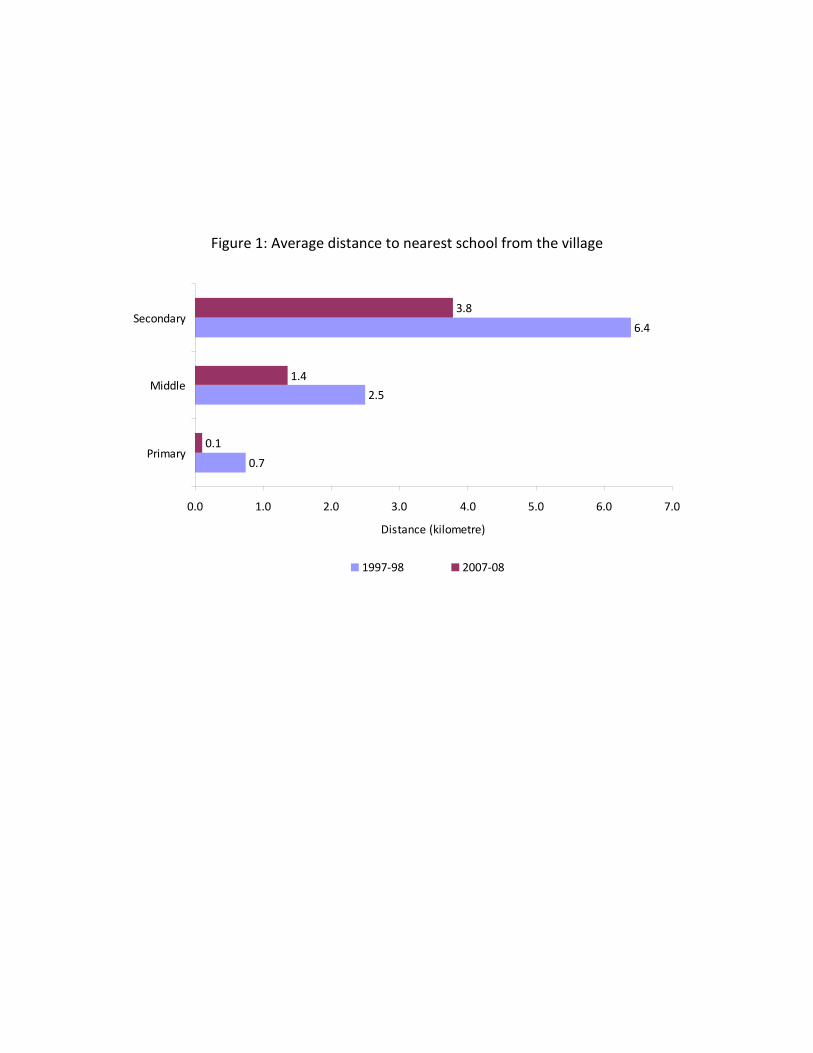
Figure 1: Average distance to nearest school from the village

0.7

2.5

6.4

0.1

1.4

3.8

0.0 1.0 2.0 3.0 4.0 5.0 6.0 7.0

Primary

Middle

Secondary

Distance (kilometre)

1997-98 2007-08

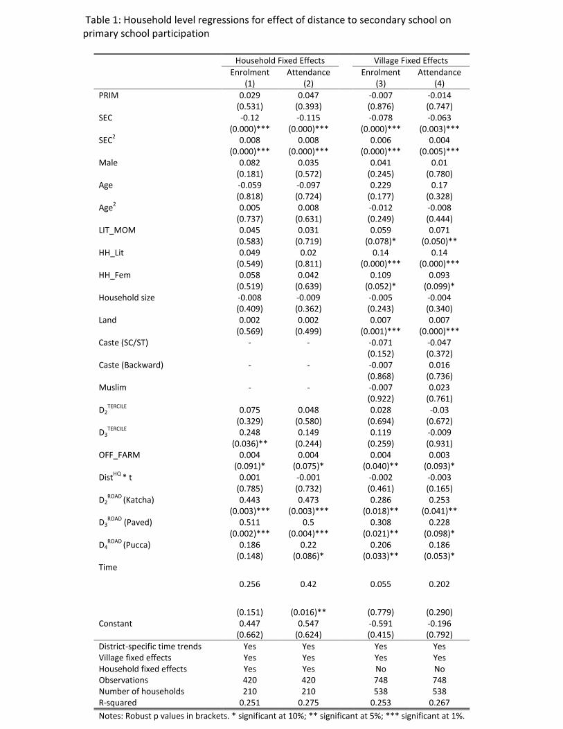
Table 1: Household level regressions for effect of distance to secondary school on primary school participation

Household Fixed Effects Village Fixed Effects Enrolment Attendance Enrolment Attendance (1) (2) (3) (4) PRIM 0.029 0.047 -0.007 -0.014 (0.531) (0.393) (0.876) (0.747) SEC -0.12 -0.115 -0.078 -0.063 (0.000)*** (0.000)*** (0.000)*** (0.003)*** SEC2 0.008 0.008 0.006 0.004 (0.000)*** (0.000)*** (0.000)*** (0.005)*** Male 0.082 0.035 0.041 0.01 (0.181) (0.572) (0.245) (0.780) Age -0.059 -0.097 0.229 0.17 (0.818) (0.724) (0.177) (0.328) Age2 0.005 0.008 -0.012 -0.008 (0.737) (0.631) (0.249) (0.444) LIT_MOM 0.045 0.031 0.059 0.071 (0.583) (0.719) (0.078)* (0.050)** HH_Lit 0.049 0.02 0.14 0.14 (0.549) (0.811) (0.000)*** (0.000)*** HH_Fem 0.058 0.042 0.109 0.093 (0.519) (0.639) (0.052)* (0.099)* Household size -0.008 -0.009 -0.005 -0.004 (0.409) (0.362) (0.243) (0.340) Land 0.002 0.002 0.007 0.007 (0.569) (0.499) (0.001)*** (0.000)*** Caste (SC/ST) - - -0.071 -0.047 (0.152) (0.372) Caste (Backward) - - -0.007 0.016 (0.868) (0.736) Muslim - - -0.007 0.023 (0.922) (0.761) D2

TERCILE 0.075 0.048 0.028 -0.03 (0.329) (0.580) (0.694) (0.672) D3

TERCILE 0.248 0.149 0.119 -0.009 (0.036)** (0.244) (0.259) (0.931) OFF_FARM 0.004 0.004 0.004 0.003 (0.091)* (0.075)* (0.040)** (0.093)* DistHQ * t 0.001 -0.001 -0.002 -0.003 (0.785) (0.732) (0.461) (0.165) D2

ROAD (Katcha) 0.443 0.473 0.286 0.253 (0.003)*** (0.003)*** (0.018)** (0.041)** D3

ROAD (Paved) 0.511 0.5 0.308 0.228 (0.002)*** (0.004)*** (0.021)** (0.098)* D4

ROAD (Pucca) 0.186 0.22 0.206 0.186 (0.148) (0.086)* (0.033)** (0.053)* Time

0.256 0.42 0.055 0.202

(0.151) (0.016)** (0.779) (0.290) Constant 0.447 0.547 -0.591 -0.196 (0.662) (0.624) (0.415) (0.792) District-specific time trends Yes Yes Yes Yes Village fixed effects Yes Yes Yes Yes Household fixed effects Yes Yes No No Observations 420 420 748 748 Number of households 210 210 538 538 R-squared 0.251 0.275 0.253 0.267

Notes: Robust p values in brackets. * significant at 10%; ** significant at 5%; *** significant at 1%.

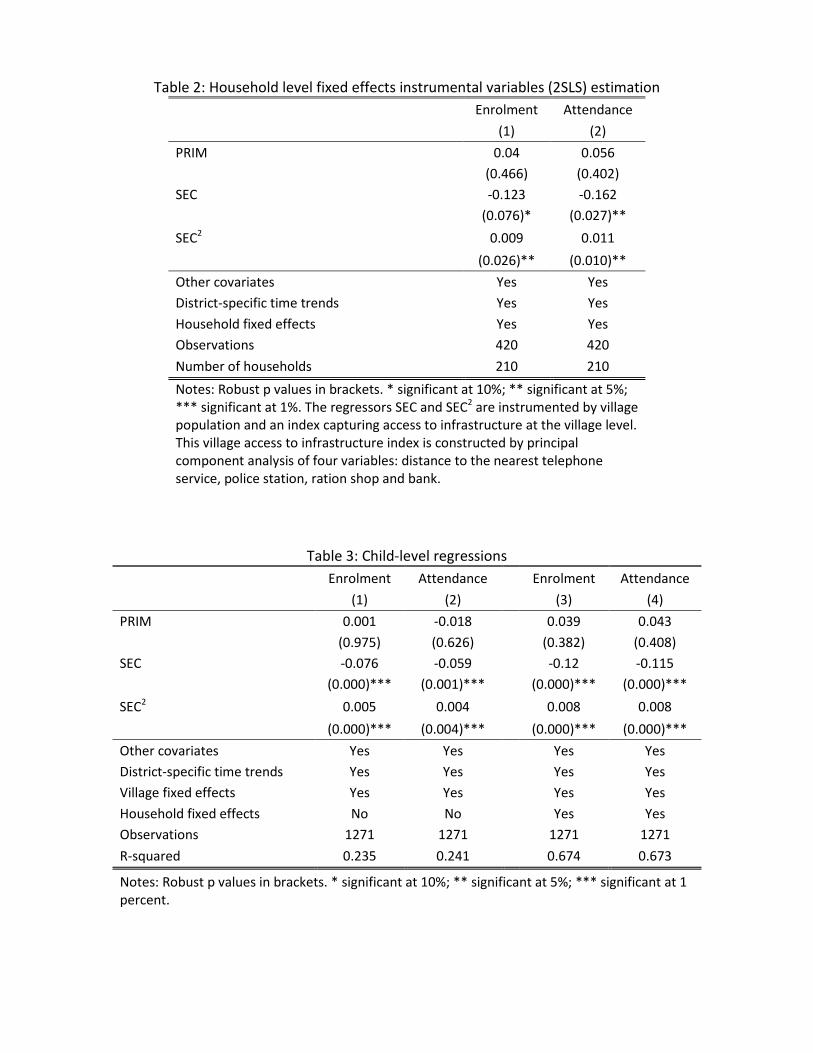
Table 2: Household level fixed effects instrumental variables (2SLS) estimation Enrolment Attendance

(1) (2)

PRIM 0.04 0.056 (0.466) (0.402) SEC -0.123 -0.162 (0.076)* (0.027)**

SEC2 0.009 0.011

(0.026)** (0.010)**

Other covariates Yes Yes District-specific time trends Yes Yes

Household fixed effects Yes Yes Observations 420 420

Number of households 210 210

Notes: Robust p values in brackets. * significant at 10%; ** significant at 5%; *** significant at 1%. The regressors SEC and SEC2 are instrumented by village population and an index capturing access to infrastructure at the village level. This village access to infrastructure index is constructed by principal component analysis of four variables: distance to the nearest telephone service, police station, ration shop and bank.

Table 3: Child-level regressions Enrolment Attendance Enrolment Attendance

(1) (2) (3) (4)

PRIM 0.001 -0.018 0.039 0.043

(0.975) (0.626) (0.382) (0.408) SEC -0.076 -0.059 -0.12 -0.115 (0.000)*** (0.001)*** (0.000)*** (0.000)***

SEC2 0.005 0.004 0.008 0.008

(0.000)*** (0.004)*** (0.000)*** (0.000)***

Other covariates Yes Yes Yes Yes District-specific time trends Yes Yes Yes Yes Village fixed effects Yes Yes Yes Yes

Household fixed effects No No Yes Yes Observations 1271 1271 1271 1271

R-squared 0.235 0.241 0.674 0.673

Notes: Robust p values in brackets. * significant at 10%; ** significant at 5%; *** significant at 1 percent.

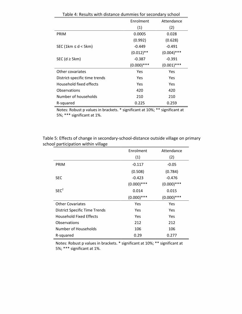
Table 4: Results with distance dummies for secondary school

Enrolment Attendance

(1) (2)

PRIM 0.0005 0.028 (0.992) (0.628) SEC (1km ≤ d < 5km) -0.449 -0.491 (0.012)** (0.004)***

SEC (d ≥ 5km) -0.387 -0.391 (0.000)*** (0.001)***

Other covariates Yes Yes District-specific time trends Yes Yes

Household fixed effects Yes Yes Observations 420 420 Number of households 210 210

R-squared 0.225 0.259


Table 5: Effects of change in secondary-school-distance outside village on primary school participation within village


(1) (2)

PRIM -0.117 -0.05

(0.508) (0.784) SEC -0.423 -0.476

(0.000)*** (0.000)***

SEC2 0.014 0.015

(0.000)*** (0.000)***

Other Covariates Yes Yes District Specific Time Trends Yes Yes

Household Fixed Effects Yes Yes Observations 212 212 Number of Households 106 106

R-squared 0.29 0.277


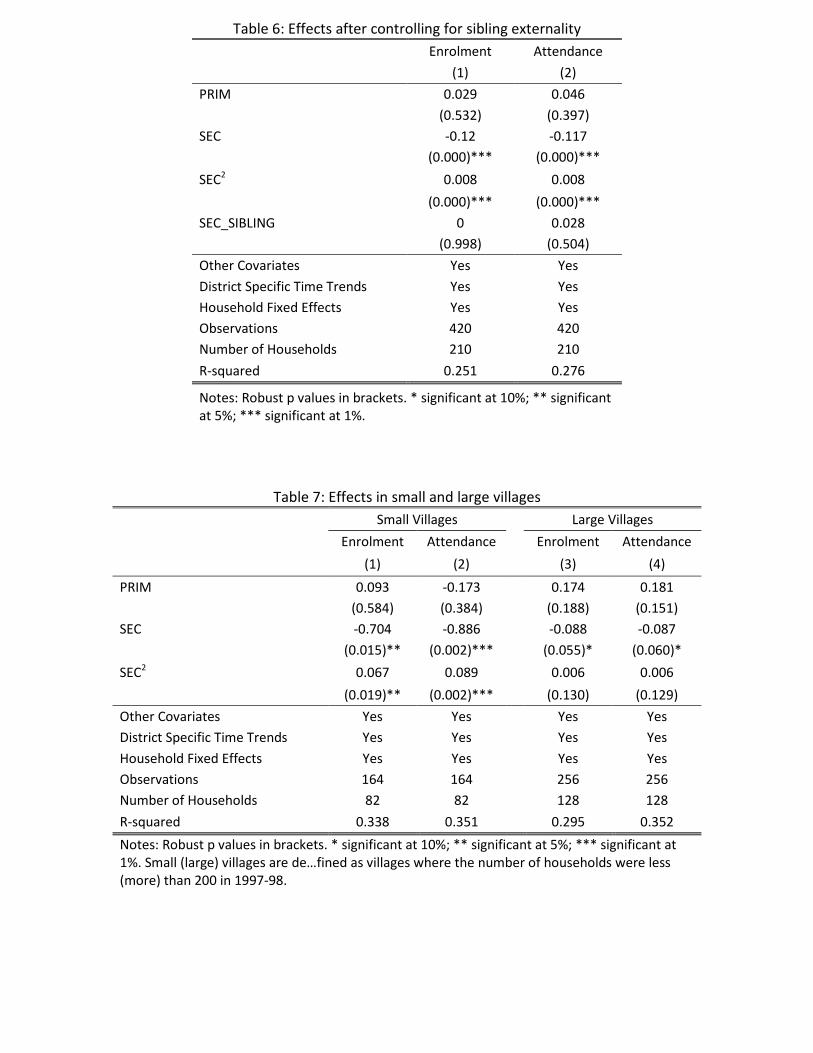
Table 6: Effects after controlling for sibling externality Enrolment Attendance

(1) (2)

PRIM 0.029 0.046

(0.532) (0.397) SEC -0.12 -0.117 (0.000)*** (0.000)***

SEC2 0.008 0.008

(0.000)*** (0.000)***

SEC_SIBLING 0 0.028 (0.998) (0.504)

Other Covariates Yes Yes

District Specific Time Trends Yes Yes Household Fixed Effects Yes Yes Observations 420 420 Number of Households 210 210

R-squared 0.251 0.276


Table 7: Effects in small and large villages Small Villages Large Villages

Enrolment Attendance Enrolment Attendance

(1) (2) (3) (4)

PRIM 0.093 -0.173 0.174 0.181 (0.584) (0.384) (0.188) (0.151) SEC -0.704 -0.886 -0.088 -0.087

(0.015)** (0.002)*** (0.055)* (0.060)*

SEC2 0.067 0.089 0.006 0.006

(0.019)** (0.002)*** (0.130) (0.129)

Other Covariates Yes Yes Yes Yes District Specific Time Trends Yes Yes Yes Yes

Household Fixed Effects Yes Yes Yes Yes Observations 164 164 256 256 Number of Households 82 82 128 128

R-squared 0.338 0.351 0.295 0.352

Notes: Robust p values in brackets. * significant at 10%; ** significant at 5%; *** significant at 1%. Small (large) villages are de…fined as villages where the number of households were less (more) than 200 in 1997-98.

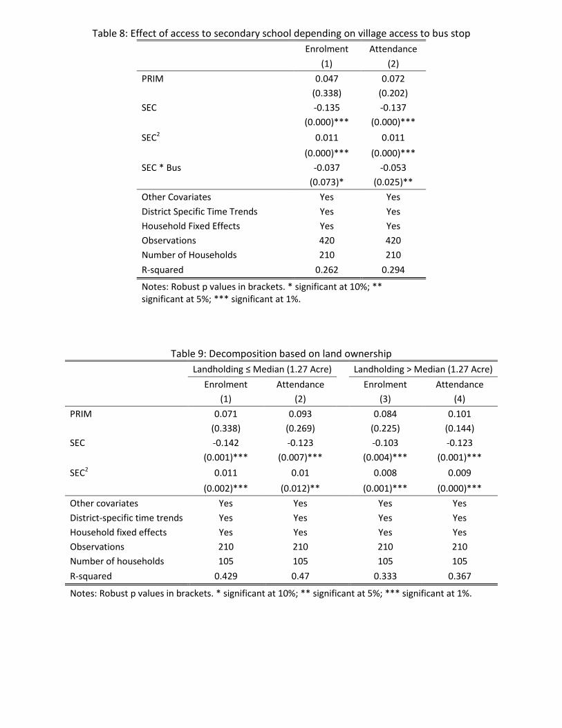
Table 8: Effect of access to secondary school depending on village access to bus stop


(1) (2)

PRIM 0.047 0.072 (0.338) (0.202) SEC -0.135 -0.137 (0.000)*** (0.000)***

SEC2 0.011 0.011

(0.000)*** (0.000)*** SEC * Bus -0.037 -0.053 (0.073)* (0.025)**

Other Covariates Yes Yes

District Specific Time Trends Yes Yes Household Fixed Effects Yes Yes Observations 420 420 Number of Households 210 210

R-squared 0.262 0.294


Table 9: Decomposition based on land ownership Landholding ≤ Median (1.27 Acre) Landholding > Median (1.27 Acre)

Enrolment Attendance Enrolment Attendance (1) (2) (3) (4)

PRIM 0.071 0.093 0.084 0.101 (0.338) (0.269) (0.225) (0.144) SEC -0.142 -0.123 -0.103 -0.123

(0.001)*** (0.007)*** (0.004)*** (0.001)***

SEC2 0.011 0.01 0.008 0.009

(0.002)*** (0.012)** (0.001)*** (0.000)***

Other covariates Yes Yes Yes Yes

District-specific time trends Yes Yes Yes Yes Household fixed effects Yes Yes Yes Yes Observations 210 210 210 210 Number of households 105 105 105 105

R-squared 0.429 0.47 0.333 0.367


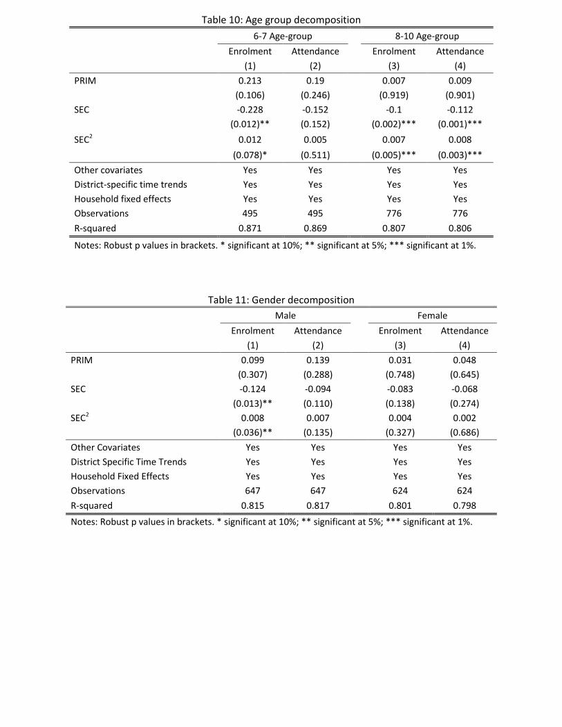
Table 10: Age group decomposition

6-7 Age-group 8-10 Age-group


(1) (2) (3) (4)

PRIM 0.213 0.19 0.007 0.009 (0.106) (0.246) (0.919) (0.901)

SEC -0.228 -0.152 -0.1 -0.112 (0.012)** (0.152) (0.002)*** (0.001)***

SEC2 0.012 0.005 0.007 0.008

(0.078)* (0.511) (0.005)*** (0.003)***

Other covariates Yes Yes Yes Yes District-specific time trends Yes Yes Yes Yes Household fixed effects Yes Yes Yes Yes Observations 495 495 776 776

R-squared 0.871 0.869 0.807 0.806


Table 11: Gender decomposition Male Female


(1) (2) (3) (4)

PRIM 0.099 0.139 0.031 0.048 (0.307) (0.288) (0.748) (0.645) SEC -0.124 -0.094 -0.083 -0.068

(0.013)** (0.110) (0.138) (0.274) SEC2 0.008 0.007 0.004 0.002 (0.036)** (0.135) (0.327) (0.686)

Other Covariates Yes Yes Yes Yes District Specific Time Trends Yes Yes Yes Yes Household Fixed Effects Yes Yes Yes Yes Observations 647 647 624 624

R-squared 0.815 0.817 0.801 0.798


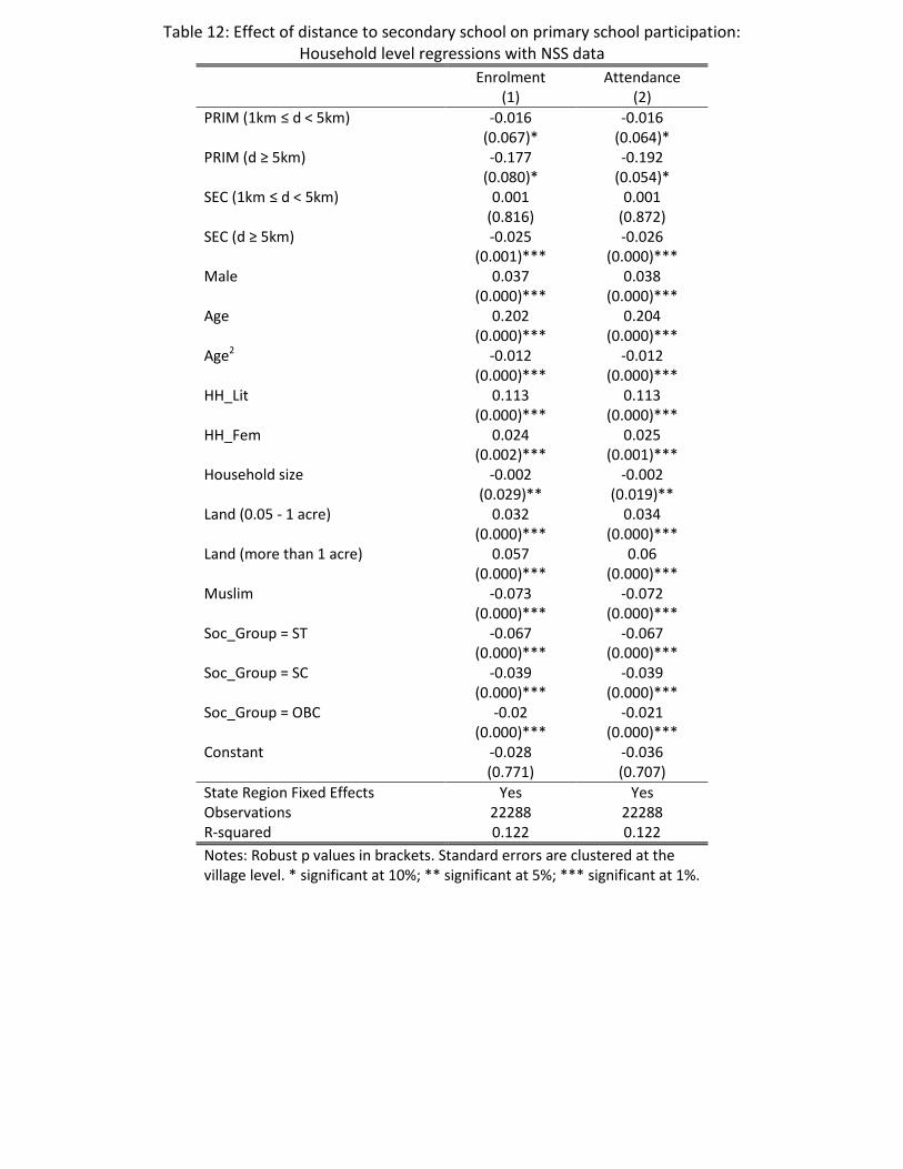
Table 12: Effect of distance to secondary school on primary school participation: Household level regressions with NSS data

Enrolment Attendance (1) (2) PRIM (1km ≤ d < 5km) -0.016 -0.016 (0.067)* (0.064)* PRIM (d ≥ 5km) -0.177 -0.192 (0.080)* (0.054)* SEC (1km ≤ d < 5km) 0.001 0.001 (0.816) (0.872) SEC (d ≥ 5km) -0.025 -0.026 (0.001)*** (0.000)*** Male 0.037 0.038 (0.000)*** (0.000)*** Age 0.202 0.204 (0.000)*** (0.000)*** Age2 -0.012 -0.012 (0.000)*** (0.000)*** HH_Lit 0.113 0.113 (0.000)*** (0.000)*** HH_Fem 0.024 0.025 (0.002)*** (0.001)*** Household size -0.002 -0.002 (0.029)** (0.019)** Land (0.05 - 1 acre) 0.032 0.034 (0.000)*** (0.000)*** Land (more than 1 acre) 0.057 0.06 (0.000)*** (0.000)*** Muslim -0.073 -0.072 (0.000)*** (0.000)*** Soc_Group = ST -0.067 -0.067 (0.000)*** (0.000)*** Soc_Group = SC -0.039 -0.039 (0.000)*** (0.000)*** Soc_Group = OBC -0.02 -0.021 (0.000)*** (0.000)*** Constant -0.028 -0.036 (0.771) (0.707) State Region Fixed Effects Yes Yes Observations 22288 22288 R-squared 0.122 0.122 Notes: Robust p values in brackets. Standard errors are clustered at the village level. * significant at 10%; ** significant at 5%; *** significant at 1%.

Appendix Table A1: Descriptive statistics of household level variables from SLC data 1997-98 2007-08

Variable Obs

. Mea

n Std. Dev.

Min Max Obs

. Mea

n Std. Dev.

Min Max

Enrol 210 0.67 0.43 0 1 210 0.83 0.35 0 1 Attend 210 0.63 0.44 0 1 210 0.82 0.35 0 1 PRIM 210 0.76 0.95 0 5 210 0.10 0.46 0 3 SEC 210 5.59 4.21 0.5 20 210 3.44 2.77 0 16 Male 210 0.38 0.49 0 1 210 0.55 0.50 0 1 Age 210 7.80 1.06 6 10 210 8.18 1.12 6 10 LIT_MOM 210 0.18 0.38 0 1 210 0.21 0.41 0 1 HH_Lit 210 0.43 0.50 0 1 210 0.47 0.50 0 1 HH_Fem 210 0.04 0.19 0 1 210 0.07 0.25 0 1 Caste (General) 210 0.16 0.37 0 1 210 0.16 0.37 0 1 Caste (SC/ST) 210 0.25 0.43 0 1 210 0.25 0.43 0 1 Caste (Backward) 210 0.59 0.49 0 1 210 0.59 0.49 0 1 Hindu 210 0.94 0.23 0 1 210 0.94 0.23 0 1 Muslim 210 0.06 0.23 0 1 210 0.06 0.23 0 1 Household size 210 8.44 3.79 3 26 210 8.43 3.02 3 19 Land 210 3.36 8.47 0 93 210 1.79 3.49 0 33 D1

TERCILE 210 0.53 0.50 0 1 210 0.06 0.24 0 1 D2

TERCILE 210 0.35 0.48 0 1 210 0.34 0.47 0 1 D3

TERCILE 210 0.12 0.32 0 1 210 0.60 0.49 0 1

OFF_FARM 210 45.1

2 29.73 2 95 210

30.43

23.71 2 90

DistHQ 210 32.6

4 16.50 7 75 210

32.64

16.50 7 75

D1ROAD (Trail only) 210 0.06 0.23 0 1 210 0.10 0.30 0 1 D2ROAD (Katcha) 210 0.31 0.46 0 1 210 0.08 0.27 0 1 D3ROAD (Paved) 210 0.31 0.46 0 1 210 0.28 0.45 0 1 D4ROAD (Pucca) 210 0.32 0.47 0 1 210 0.54 0.50 0 1

Village population 210 1966 1118 351 519

5 210 3383 1885 369

8040

Village distance index

210 0.19 1.30 -

1.59 4.37 210 -0.47 0.84

-1.59

2.76

Source: Survey of Living Condition (SLC) data

Appendix Table A2: First stage results of 2SLS estimation (Table 2) Dependent Variable SEC SEC2 (1) (2) Village Population 0.001 0.006 (0.001)*** (0.117) Infrastructure 1.236 28.752 (0.014)** (0.000)*** Other Covariates Yes Yes District Specific Time Trends Yes Yes Household Fixed Effects Yes Yes Observations 420 420 Number of Households 210 210 R-squared 0.638 0.803 F-stat 18.41 27.34


does access to secondary education affectftp.iza.org/dp6507.pdfdoes access to secondary education...

Documents